ONDA 1.4 USER’S MANUAL Version 1.4

by Prof. D.C.F. Lo Presti & Eng. S. Stacul

1 INTRODUCTION ONDA

This user’s manual describes how to use a newly developed computer code for

performing One-dimensional Non-linear Dynamic Analysis (ONDA) of soil deposits.

The code has been developed by revisiting the work by Ohsaki (1982) and extending

its capabilities to model important aspects of soil non-linear response when subjected

to earthquake loading like for instance the phenomenon of cyclic degradation. In the

Ohsaki model a horizontally stratified soil deposit is idealized as a discrete mechanical

system composed by a finite number of lumped masses connected with a series of

springs and dashpots. Non-linearity is modeled by assuming 1) a “backbone” curve

that describes the initial, monotonic loading of the stress-strain curve, and 2) a “rule”

that simulates the unloading-reloading paths and stiffness degradation undergone by

soil as seismic excitation progresses.

Typically, the backbone curve is obtained from conventional cyclic undrained

loading laboratory tests. For the “rule” it is generally used the so-called “Masing

criterion” which assumes that the unload-reload branches of the stress-strain curve

have the same shape of the initial loading curve but affected by a scale factor (n) equal

to 2. ONDA assumes a modified 2nd Masing criterion, which considers a scale factor

(n) not necessarily equal to 2. It turns out that a factor n greater than 2 allows to simulate

the phenomenon of cyclic hardening, while cyclic softening can be modeled by

assuming values of n smaller than 2. This generalization of the Masing criterion allows

to proper simulate the phenomena of soil hardening and soil degradation giving to

ONDA the capability to compute the permanent shear strains developed during a

seismic event. Description of the procedure required to evaluate the model-parameters

is also given in the manual.

In ONDA the numerical solution of the non-linear equations of motion is

obtained using the unconditionally stable Wilson θ algorithm (with θ >1.37).

The version 1.0 of the code has been developed by Camelliti (1999) and assume

the n parameter arbitrarily but constant. Version 1.0 has been used in some applications

(Vercellotti 2001, De Martini Ugolotti 2001, Saviolo 2002). The version 1.3 (Lo Presti

et al. 2003) offers the possibility of selecting initial values of the n parameter and its

variation with strain and number of cycles.

The actual version 1.4 in addiction gives the possibility to select α and R

parameters.

2 ONE-DIMENSIONAL GROUND RESPONSE ANALYSIS

One-dimensional ground response analysis introduces some restrictive

hypotheses on geometry and wave field kinematics, which are discussed in this chapter.

Nonetheless these restrictions, 1D analyses have been successfully used in many cases

and more specifically: a) when topographic irregularities are absent, b) when the effects

of the boundaries of the sedimentary valleys or of deeper geologic structures can be

neglected.

2.1 Geometry and kinematics assumptions

One dimensional ground response analyses are based on the following assumptions:

• horizontally stratified soil layers;

• soil strata and bedrock extend infinitely in the horizontal direction;

• the only waves traveling into the soil deposits are SH waves propagating

vertically from the underlying bedrock.

2.2 Input motion, bedrock and outcropping motion

Figure 1 recalls common accepted terminology to define ground motion. The

main objective of seismic response analysis is the analytical determination of the free

surface motion, i.e. the motion at the surface of a soil deposit. The motion at the base

of the soil deposit (top of the bedrock) is called bedrock motion. The rock outcropping

motion is the motion at a location where bedrock is exposed at the ground surface.

In the case of infinitely stiff base, bedrock and rock outcropping motions

coincide. In the case of compliant base, these motions do not coincide because of

radiation damping in the rock. The way of considering compliant base (i.e. radiation

condition) in ONDA is described in the sequel.

Figure 1 Ground response nomenclature

3 THE PROGRAM ONDA

3.1 General features of the code

ONDA is a computer code designed to perform one-dimensional non-linear

ground response analysis of horizontally stratified soil deposits. The code has been

developed following the model by Ohsaki (1982) where the soil deposit is modeled as

a discrete system composed by a finite number of lumped masses connected weakly

with springs and dashpots (see Fig 2). Weak coupling among the lumped masses yields

a characteristic three-diagonal, banded stiffness and a consistent mass matrix (Ohsaki,

1982). The equation of motion governing the vibrations of the discrete system

subjected to a base acceleration �̈�𝑦 can be written as follows:

𝑴𝑴�̈�𝒙 + 𝑪𝑪�̇�𝒙 + 𝑲𝑲𝒙𝒙 = −�̈�𝒚𝑴𝑴 ∙ 𝒓𝒓

(1)

where x is the horizontal displacement vector (see Fig. 2), r is a unit vector, M is the

consistent mass matrix formed by terms proportional to 𝜌𝜌𝑗𝑗𝐻𝐻𝑗𝑗 with 𝜌𝜌𝑗𝑗 being the mass

density of the jth layer having thickness 𝐻𝐻𝑗𝑗 and 𝑗𝑗 = 1,𝑁𝑁. C is the Rayleigh damping

matrix, and K the stiffness matrix formed by terms proportional to 𝐺𝐺𝑗𝑗 𝐻𝐻𝑗𝑗⁄ with 𝐺𝐺𝑗𝑗 being

the strain dependent shear modulus associated to the jth layer. N is the number of

sublayers in which the soil deposit has been subdivided. Further details on the structure

of the stiffness and damping matrices appearing in Eq. (1) with the precise definition

of the elements Ki,j and Ci,j are provided in Oshaki (1982) and will not be reported here.

The input motion is assigned at the base of the mechanical system (see Fig. 2c) where

the bedrock is assumed to have a finite stiffness. The radiation condition in the half-

space as well as the possibility that the input motion be assigned as an outcropping

motion is modelled through the standard concept of energy-transmitting boundary

(Joyner and Chen, 1975; Oshaki, 1982). This essentially consists in inserting at the

base of the soil deposit a fictitious dashpot with damping coefficient equal to �𝜌𝜌𝑏𝑏𝐺𝐺𝑏𝑏

where 𝜌𝜌𝑏𝑏 and 𝐺𝐺𝑏𝑏 are the mass density and the tangent shear modulus of the sub-stratum.

Equation (1) is non-linear because of the strain dependence of the elements of K. It

was solved by integration in the time domain using the Wilson θ-method, which is

recalled to be unconditionally stable for θ >1.37 (Chopra, 1995).

The program ONDA computes the time history of acceleration, relative velocity

and relative displacement at a specific sub-layer (either outcropping or not), the

corresponding Fourier and elastic response spectra, the time history of stress, strain and

stress-strain loops at a specified sub-layer (either outcropping or not), and the

horizontal permanent deformations undergone by a specific sub-layer (either

outcropping or not) at the end of the seismic excitation.

Figure 2 Discrete system

3.2 Non-linear cyclic constitutive modeling

The constitutive model adopted by ONDA employs for the description of the

initial loading stress-strain curve (backbone or skeleton curve) the Ramberg-Osgood

(1943) model. The cyclic behaviour of unloading-reloading (hysteretic curves) has

been modelled using the modified second Masing criterion (Tatsuoka et al., 1993) (see

Fig. 3). Such a criterion represents the most innovative aspect of the constitutive model

and hence of the computer code.

Figure 3 Geometrical formation of hysteretic curve

It will be described in the sequel. Firstly it is worthwhile to resume the three basic

rules that are assumed for the non-linear model:

• 1st rule: the stress-strain curve is the backbone curve until the appearance of the

first stress reversal;

• 2nd rule: the stress-strain curves (hysteretic curves), after the stress-reversal,

follow the modified second Masing criterion;

• 3rd rule: beyond the terminal point of a hysteretic curve, the stress-strain curve

follows the second latest hysteretic curve. The stress-strain curve resumes the

backbone curve in two special cases: a) when the latest curve is the backbone

curve and b) when the second latest curve is the backbone curve. This third rule

coincides in practice with the additional criteria postulated by Pyke (1979).

The expression of Ramberg-Osgood (1943) is represented by a non-invertible power

relation depending on four parameters. The parameters α and 𝑅𝑅 describe position and

curvature respectively. The other parameters are 𝜏𝜏𝑚𝑚𝑚𝑚𝑚𝑚 (soil shear strength) and 𝐺𝐺0 (the

low-strain shear modulus). For fine-grained soils, 𝜏𝜏𝑚𝑚𝑚𝑚𝑚𝑚 can be determined from the

undrained shear strength1. The relation can be written as follows:

𝑥𝑥 = 𝑦𝑦 ∙ (1 + 𝛼𝛼 ∙ |𝑦𝑦|𝑅𝑅−1)

(2)

where x and y are the normalized strains and stresses respectively. In particular, 𝑥𝑥 =

𝛾𝛾 𝛾𝛾𝑅𝑅𝑅𝑅𝑅𝑅⁄ and 𝑦𝑦 = 𝜏𝜏 𝜏𝜏𝑚𝑚𝑚𝑚𝑚𝑚⁄ . In these definitions 𝜏𝜏 is the shear stress, 𝛾𝛾 is the engineering

shear strain, 𝛾𝛾𝑅𝑅𝑅𝑅𝑅𝑅 = 𝜏𝜏𝑚𝑚𝑚𝑚𝑚𝑚 𝐺𝐺0⁄ .

The parameters 𝛼𝛼 and 𝑅𝑅 of Eq. (2) are determined from a regression on

experimental data obtained from a monotonic loading test or the first quarter of cycle

of cyclic tests. The parameter 𝜏𝜏𝑚𝑚𝑚𝑚𝑚𝑚 can be experimentally determined from laboratory

tests as 𝛼𝛼 and 𝑅𝑅. The parameter 𝐺𝐺0 can also be determined from laboratory tests if there

is availability of high quality samples. However, it is recommended to obtain G0 from

in situ geophysical tests.

The Ramberg-Osgood (1943) model associated to the Masing (1926) criteria

allows representing the unloading-reloading branches of the stress-strain relationship

as follows:

𝑥𝑥 − 𝑥𝑥𝑐𝑐𝑛𝑛

=𝑦𝑦 − 𝑦𝑦𝑐𝑐𝑛𝑛

∙ �1 + 𝛼𝛼 ∙ �𝑦𝑦 − 𝑦𝑦𝑐𝑐𝑛𝑛

�𝑅𝑅−1

�

(3)

where 𝑥𝑥𝑐𝑐 and 𝑦𝑦𝑐𝑐 are respectively the normalized strain and stress amplitude at the

loading reversal point of the stress-strain loop. In particular, according to the Masing

criterion the unloading-reloading curves have the same shape as the backbone curve

but they are enlarged by a scale factor of 2. In ONDA however, it was adopted the

modified second Masing criterion (Tatsuoka et al., 1993) for which the above scale

factor may virtually assume an arbitrary value n. In particular, to simulate cyclic

hardening behavior it will be necessary to assume a scale factor n > 2, whereas cyclic

softening or material degradation could be modeled by assuming decreasing values of

n even n < 2. It is then possible by assuming the scale factor n as a function of the

number of cycles N, and of the strain level to fully describe some of the most relevant

aspects of soil non-linear behavior including those arising from the increase of pore

water pressure, even though indirectly because the analysis is conducted in terms of

total stresses.

If 𝐺𝐺𝑒𝑒𝑒𝑒 is the unloading-reloading shear modulus from cyclic tests, and 𝐺𝐺𝑠𝑠 is the

secant shear modulus from monotonic tests or the first quarter of cycle of cyclic tests,

the specific sequence of n values adopted by ONDA is obtained experimentally from

the condition 𝐺𝐺𝑒𝑒𝑒𝑒 = 𝐺𝐺𝑠𝑠. More precisely, the sequence of n-values is determined from

the expression 𝑛𝑛 = 2𝛾𝛾𝑐𝑐 𝛾𝛾⁄ where 𝛾𝛾𝑐𝑐 and 𝛾𝛾 and are respectively the cyclic and

monotonic shear strain values for which the relationship 𝐺𝐺𝑒𝑒𝑒𝑒 = 𝐺𝐺𝑠𝑠 holds (Tatsuoka et

al. 1993) (see fig. 4 a, b, c).

Figure 4 Assessment of n parameter (a) and comparison between model prediction (b) and

experimentally determined stress strain loops (c)

It is recalled that in ONDA and in general in computer codes based on modelling

the non-linear behaviour through the association of an initial loading backbone curve

with a “rule” that simulate the unloading-reloading cyclic response with or without

cyclic hardening or softening, the phenomenon of energy dissipation is reproduced

implicitly in the analysis through the updating of the stiffness matrix K (see Eq. 1) as

the loading history progresses (Camelliti, 1999). Such type of constitutive behavior is

borrowed from the general theory hypoelasticity (Lubliner, 1990), which even though

is questionable from the thermodynamical point of view, it is not the cause of too severe

shortcomings in the engineering applications. This hypoelastic, built-in mechanism of

energy dissipation in ONDA, is superimposed to a second mechanism which is the one

associated to the damping matrix C of Eq. (1). Of much lesser importance, this energy

dissipation mechanism is associated to a damping of a viscous nature (i.e. frequency

dependent) and it is effective only at very low strain levels, below the linear cyclic

threshold shear strain (Vucetic, 1994). At larger strain, this second mechanism still

holds but represent a very small percentage in comparison to the hysteretic mechanism.

3.3 Spatial discretization and time integration algorithms

Horizontally stratified soil deposits are modeled as a discrete system composed

by a finite number of lumped masses connected weakly with springs and dashpots (see

Fig 2). Macro-layers are identified through the geotechnical profile and are

characterized by a set of constitutive parameters. For the step-by-step integration of the

equations of motion [1] ONDA has adopted the Wilson θ method which is

unconditionally stable for 𝜃𝜃 ≥ 1.37 (Chopra, 1995). Details about the application of

the Wilson θ method can be found in any textbook on structural dynamics and will not

be reported here. At the time t, the equations of motion [1] can be re-written in the

following incremental form:

�𝑲𝑲��𝒕𝒕{𝚫𝚫𝒙𝒙}𝒕𝒕 = {𝑹𝑹}𝒕𝒕

(4)

where {𝚫𝚫𝒙𝒙}𝒕𝒕 is the incremental displacement vector at time t, and the matrices �𝑲𝑲��𝒕𝒕

and �𝑹𝑹��𝒕𝒕 are defined by the following relationships:

�𝑲𝑲��𝑡𝑡 =6𝜏𝜏2𝑴𝑴 +

3𝜏𝜏𝑪𝑪 + {𝑲𝑲}𝑡𝑡

(5a)

{𝑹𝑹}𝑡𝑡 = 𝑴𝑴 ∙ �Δ𝑅𝑅𝑡𝑡𝑰𝑰 +6𝜏𝜏

{�̇�𝒙}𝑡𝑡 + 3{�̈�𝒙}𝑡𝑡� + 𝑪𝑪 ∙ �3{�̇�𝒙}𝑡𝑡 +𝜏𝜏2

{�̈�𝒙}𝑡𝑡�

(5b)

where {𝑲𝑲}𝑡𝑡 is the stiffness matrix of Eq.[1] updated at time t, 𝑰𝑰 is the identity matrix,

𝜏𝜏 = 𝜃𝜃 ∙ Δ𝑡𝑡, and Δ𝑅𝑅𝑡𝑡 = −𝜃𝜃(�̈�𝑦𝑡𝑡+Δ𝑡𝑡 − 𝑦𝑦�̈�𝑡). Once Eq.[4] is solved, the acceleration,

velocity and displacement vectors {�̈�𝒙}𝑡𝑡+Δ𝑡𝑡, {�̇�𝒙}𝑡𝑡+Δ𝑡𝑡, {𝒙𝒙}𝑡𝑡+Δ𝑡𝑡 at time 𝑡𝑡 + Δ𝑡𝑡 can be

computed by means of the following relations:

{�̈�𝒙}𝑡𝑡+Δ𝑡𝑡 =6𝜏𝜏2𝜃𝜃

{𝚫𝚫𝒙𝒙}𝑡𝑡 −6𝜏𝜏𝜃𝜃

{�̇�𝒙}𝑡𝑡 + �1 −3𝜃𝜃� {�̈�𝒙}𝑡𝑡

(6a)

{�̇�𝒙}𝑡𝑡+Δ𝑡𝑡 = {�̇�𝒙}𝑡𝑡 +Δ𝑡𝑡2

[{�̈�𝒙}𝑡𝑡+Δ𝑡𝑡 + {�̈�𝒙}𝑡𝑡]

(6b)

{𝒙𝒙}𝑡𝑡+Δ𝑡𝑡 = {𝒙𝒙}t + Δ𝑡𝑡{�̇�𝒙}𝑡𝑡 +(Δ𝑡𝑡)2

6[{�̈�𝒙}𝑡𝑡+Δ𝑡𝑡 + 2{�̈�𝒙}𝑡𝑡]

(6c)

From the knowledge of the displacement vector, the strain and the stress vectors can

be straightforwardly calculated.

4 SYSTEM REQUIREMENT

• Windows XP, Windows Vista, Windows 7 or newer

• 32 or 64 bit

• Minimum 3 GB disk space to download and install

4.1 Python environment

ONDA 1.4 has been developed in Python language. The program is available in

an executable format. Not preliminary installation of python is required to run ONDA

1.4.

4.2 Installing and removing ONDA

To install the application run the executable file and follow the instructions. To

remove the application, go to “Control Panel” “Programs and Features” and

uninstall the application.

5 RUNNING ONDA

To perform a ground response analysis with ONDA it’s necessary to create 4 tab-

delimited txt files (input data):

1. the first to load the soil profile;

2. the second to load the values of soil cohesion c’ (in kPa);

3. the third to load the values of the angle of friction 𝜑𝜑′ (in degrees);

4. the fourth to load the input motion (acceleration in g).

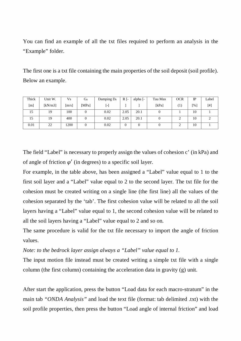
You can find an example of all the txt files required to perform an analysis in the

“Example” folder.

The first one is a txt file containing the main properties of the soil deposit (soil profile).

Below an example.

Thick

[m]

Unit W.

[kN/m3]

Vs

[m/s]

G0

[MPa]

Damping D0

[-]

R [-

]

alpha [-

]

Tau Max

[kPa]

OCR

(1)

IP

[%]

Label

[#]

15 19 100 0 0.02 2.05 20.1 0 1 10 1

15 19 400 0 0.02 2.05 20.1 0 2 10 2

0.01 22 1200 0 0.02 0 0 0 2 10 1

The field “Label” is necessary to properly assign the values of cohesion c’ (in kPa) and

of angle of friction 𝜑𝜑′ (in degrees) to a specific soil layer.

For example, in the table above, has been assigned a “Label” value equal to 1 to the

first soil layer and a “Label” value equal to 2 to the second layer. The txt file for the

cohesion must be created writing on a single line (the first line) all the values of the

cohesion separated by the ‘tab’. The first cohesion value will be related to all the soil

layers having a “Label” value equal to 1, the second cohesion value will be related to

all the soil layers having a “Label” value equal to 2 and so on.

The same procedure is valid for the txt file necessary to import the angle of friction

values.

Note: to the bedrock layer assign always a “Label” value equal to 1.

The input motion file instead must be created writing a simple txt file with a single

column (the first column) containing the acceleration data in gravity (g) unit.

After start the application, press the button “Load data for each macro-stratum” in the

main tab “ONDA Analysis” and load the text file (format: tab delimited .txt) with the

soil profile properties, then press the button “Load angle of internal friction” and load

the angle of friction values, then press the button “Load cohesion” and load the

cohesion values and then load the input motion using the “Load accelerogram” button.

After that, insert manually in the main tab “ONDA Analysis” the following input data:

• Scale Factor [-] = insert the scale factor that you want to apply to scale the input

motion. Use a scale factor equal to 1 if you don’t want to scale the accelerogram

used;

• Time interval [in sec] = the sampling time of the input motion (the accelerogram

in the example folder has a sampling time equal to 0.005 sec);

• Time interval subdivision = insert an integer number. Equal to 1 if you want to

maintain the time interval equal to the sampling time, bigger than 1 if you want

to subdivide every time interval in N time sub-intervals. If you are performing a

Linear ground response analysis it’s recommended to use a Time interval

subdivision equal to 1; if you are performing a Non-Linear analysis it’s strongly

suggested to use a bigger value (for common situations a Time interval

subdivision value equal to 4 should be appropriate to obtain the convergence of

the solution);

• Number of macro-strata including the base layer (or bedrock) = is the total

number of layers in the soil profile. In the example above the number of layers

is 3 (including the bedrock);

• Water table depth [in meters] = specify here the water table depth;

• Type of ONDA analysis = insert 1 if you want to perform a non-linear analysis

in time domain, insert 0 if you want to perform a linear analysis;

• Procedure for n (Masing) = enter 1 if you want to consider n variable; enter 0 if

you want to consider n constant;

• Input Motion type = enter 1 if the input motion is an outcrop motion; enter 0 if

the input motion is a within motion;

• Damping ratio elastic response spectrum [in %] = specify the damping ratio

value for the calculation of the elastic response spectrum;

• Output-Result Depth [in meter] = enter the depth at which you prefer to

automatically obtain the main output plots (acceleration time history, fourier

spectrum and elastic response spectrum);

Then press the “Verify Input” button to import all the values inserted manually and to

check if they are correct. Finally, you can press the “Start analysis” button. If the

analysis has been correctly executed the message “Analysis completed” will appear in

the same row of the Start Analysis button.

Using the next tabs “Accelerogram”, “Fourier spectrum”, “Elastic R-Spectrum”,

“Strain and Displ Time History”, “Peak Profiles”, “Stress-Strain”, “Permanent displ”

and “Other Outputs”, you can plot all the results of the seismic response analysis. In

these tabs there are 2 “Plot” buttons. The first one called “Plot …. Viewer” works only

to plot the results of an analysis already performed, using the txt files saved. The second

one called “Plot ….”, instead, works only to see the results obtained in the current

analysis. The zoom, pan and home buttons instead works in both cases.

5.1 Input parameters: additional information

If 𝐺𝐺0 is not defined (zero values in the fourth column of the txt file containing

the main properties of the soil deposit), the values of the small strain shear modulus

are computed from the shear wave velocities.

If 𝜏𝜏𝑚𝑚𝑚𝑚𝑚𝑚 is not given (zero values in the column n°8 of the txt file containing the

main properties of the soil deposit), it is computed in the following way:

𝜏𝜏𝑚𝑚𝑚𝑚𝑚𝑚 = 𝑐𝑐′ + 𝜎𝜎𝑣𝑣′ ∙ tan𝜑𝜑′

(7)

where: 𝑐𝑐′ and 𝜑𝜑′ are the parameters of the Mohr-Coulomb failure envelope defined by

the vectors fi and cp for the different types of materials; 𝜎𝜎𝑣𝑣′= vertical effective geostatic

stress at middle height of each layer.

OCR and plasticity index are assumed to affect the value of the parameter n and

its dependence on number of cycles and cyclic shear strain will be shown in the next

section.

5.1.1 Constitutive parameters

To perform a ground response analysis ONDA requires the following constitutive

parameters:

• the Ramberg-Osgood parameters 𝜏𝜏𝑚𝑚𝑚𝑚𝑚𝑚, 𝐺𝐺0, α and 𝑅𝑅 to define the backbone

curve.

• scale amplification factor (n) and its variation with strain level and number of

cycles.

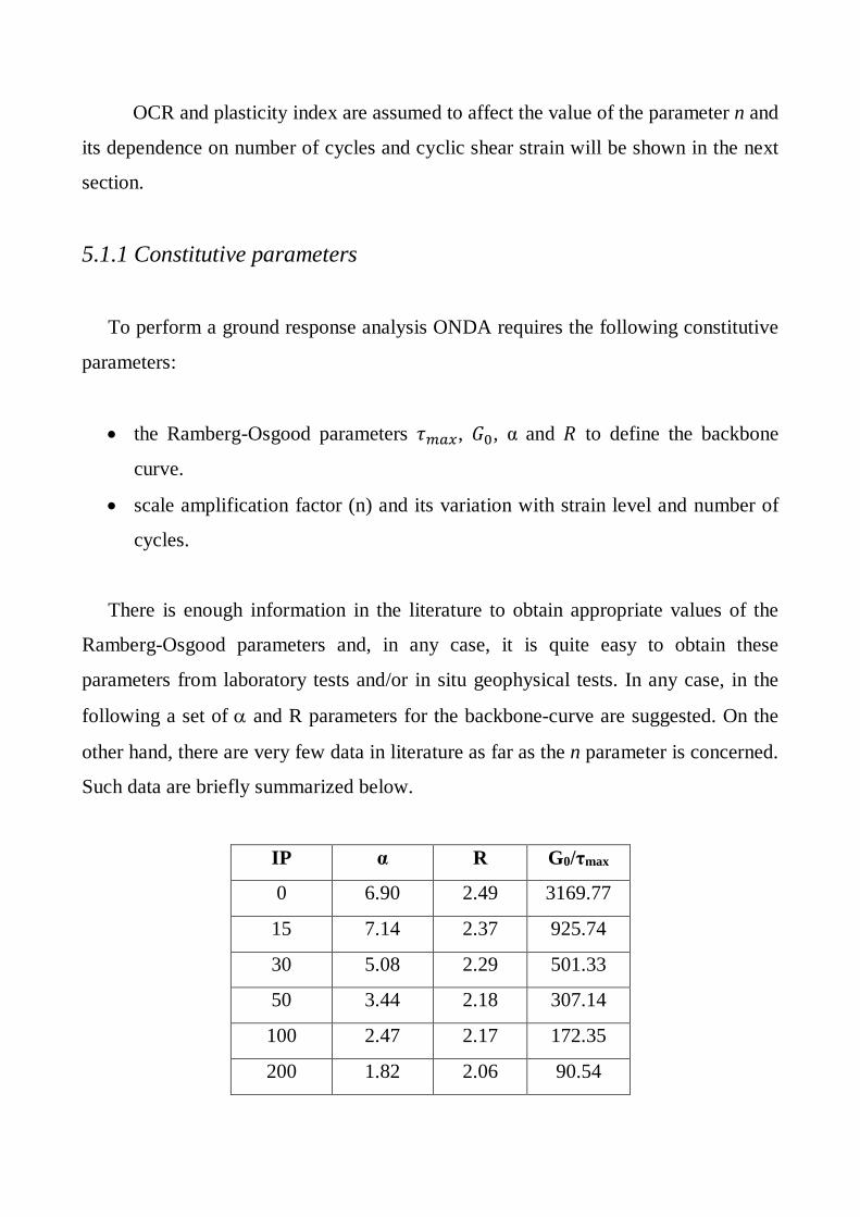
There is enough information in the literature to obtain appropriate values of the

Ramberg-Osgood parameters and, in any case, it is quite easy to obtain these

parameters from laboratory tests and/or in situ geophysical tests. In any case, in the

following a set of α and R parameters for the backbone-curve are suggested. On the

other hand, there are very few data in literature as far as the n parameter is concerned.

Such data are briefly summarized below.

IP α R G0/τmax

0 6.90 2.49 3169.77

15 7.14 2.37 925.74

30 5.08 2.29 501.33

50 3.44 2.18 307.14

100 2.47 2.17 172.35

200 1.82 2.06 90.54

Lo Presti et al. (1998, 2000) have compared the results of cyclic loading torsional shear

tests (CLTST) or Resonant Column tests (RCT) to those of monotonic loading torsional

shear tests (MLTST), both performed on the same specimen in undrained conditions.

In particular, the MLTST stage was run after CLTST. A rest period of 24 hours, with

open drainage, took place between two stages. The tests were run on some Italian clays

of medium to high plasticity, having OCR from 1.5 to 5 and the maximum applied

single amplitude shear strain was typically less than 0.05%. The above described

experiments and comparisons led to values of n ranging mainly from 4 to 6.

Ionescu (1999) performed similar tests on reconstituted Toyoura sand specimens

clarifying the following aspects:

• at very small strains (𝛾𝛾 ≤ 0.001%) n is typically equal to 2;

• the value of n increases up to 6 with the increase of shear strain (not exceeding

0.05%);

• for a given strain level n increases with the number of loading cycles. Stable

values of n are reached after 5 cycles.

The above reported results clearly indicate that: i) at very small strains the secant

stiffness coincides with that inferred from cyclic tests, which involves a quasi-elastic

behaviour at small strains (Tatsuoka and Shibuya 1992); ii) at larger strains (less than

0.05%) the stiffness from cyclic tests is greater than the secant stiffness, which involves

cyclic hardening for both clays and sands (Tatsuoka and Shibuya 1992).

The results of 23 undrained cyclic triaxial tests performed on 𝐾𝐾0 consolidated

specimens have been analyzed on the purpose of obtaining more precise indication

about the values of the n parameter (Rigazio 2001, Pallara and Lo Presti 2002). Test

specimens were 70 mm in diameter and 140 mm in height. Apparatuses were equipped

for local strain measurements. Dry setting method and automatic 𝐾𝐾0 consolidation

procedure with a tolerance on radial displacement of ±0.5 𝜇𝜇m were adopted (Lo Presti

et al., 1999). Cyclic loading was carried out by six steps. Each step involved 30 cycles

at constant strain and strain rate (triangular wave form). The strain levels, imposed to

the specimen, in the different steps, were equal to 0.003 – 0.01 - 0.02 – 0.05 – 0.1 –

0.3%. After cyclic loading, the specimen experienced a rest period of 24 hours with

opened drainage. After that it was subjected to undrained monotonic loading. Most of

the tested specimen were NC but some were OC with OCR in between 2 and 4.

Figure 5 𝑛𝑛0 vs strain level: a) influence of soil type and Ip; b) influence of OCR

The secant stiffness, measured during the first quarter of cycle or from the

subsequent monotonic loading, has been compared to the unloading-reloading stiffness

obtained from the subsequent cycles. The following experimental evidences were

established from such a comparison:

• the initial value of 𝑛𝑛 (𝑛𝑛0) depends on strain level and the type of soil (Figures 5a

and 5b). Such a parameter has been obtained by comparing the secant stiffness

from first quarter of loading to that inferred from the first cycle of unloading

reloading;

• at very small strains 𝑛𝑛0 is very close to 2 (Figure 5a);

• the values of 𝑛𝑛0 increase from 2 to a maximum value of 6 with an increase of

the axial strain up to a certain value; for strain level greater than such a limit 𝑛𝑛0

decreases to a minimum value of about 2.5 (Figure 5b). The strain level at which

𝑛𝑛0 starts to decrease is equal to about 0.1% even though it depends on soil

plasticity and possibly on OCR. More specifically, such a threshold strain level

decreases with a decrease in the plasticity index (Figure 5a), in agreement with

the concept of volumetric threshold strain and related experimental findings

(Vucetic 1994);

• smaller values of 𝑛𝑛0 are observed in the case of overconsolidated soils, that is

soils with 2<OCR<4 (Figure 5b);

• The variation of 𝑛𝑛 with the number of cycles (N), for a given strain level, has

been expressed by the following empirical relation (Figure 6a):

log(𝑛𝑛) = log(𝑛𝑛0) − 𝑡𝑡∗ ∙ log(𝑁𝑁)

(8)

• where the parameter t* appearing in Eq. 8 describes the decrease of n with the

number of loading cycles for a given strain level. Hence t* represents a sort of

degradation parameter and 𝛿𝛿 = 𝑛𝑛 𝑛𝑛0⁄ is the degradation index at very small

strains, n is independent of N (i.e. t*=0). Idriss et al. (1978) proposed the

degradation parameter t defined by Eq. 9 (Figure 6b):

log(𝐸𝐸𝑁𝑁) = log(𝐸𝐸1) ∙ log(𝑁𝑁)

(9)

where 𝐸𝐸𝑁𝑁 is the stiffness at the nth cycle and 𝐸𝐸1 is that of the 1st cycle.

The values of t* and t have been compared in Figure 7. A clear correlation exists,

and, on average, t*=1.45 t.

Figure 6 Degradation parameters: a) as defined in this manual; b) according to Idriss et al. (1978)

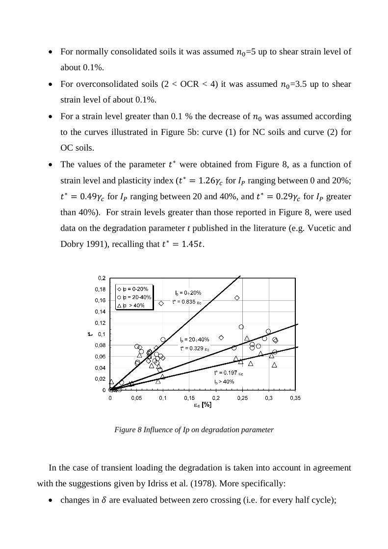
• The values of t*, obtained from the testing campaign, are summarized in Figure

8. They mainly depend on plasticity index and, for a given soil, on strain level.

Therefore, the values of t* can be obtained from Figure 8, as a function of strain

level and plasticity index; in particular for the data of Figure 8, the following

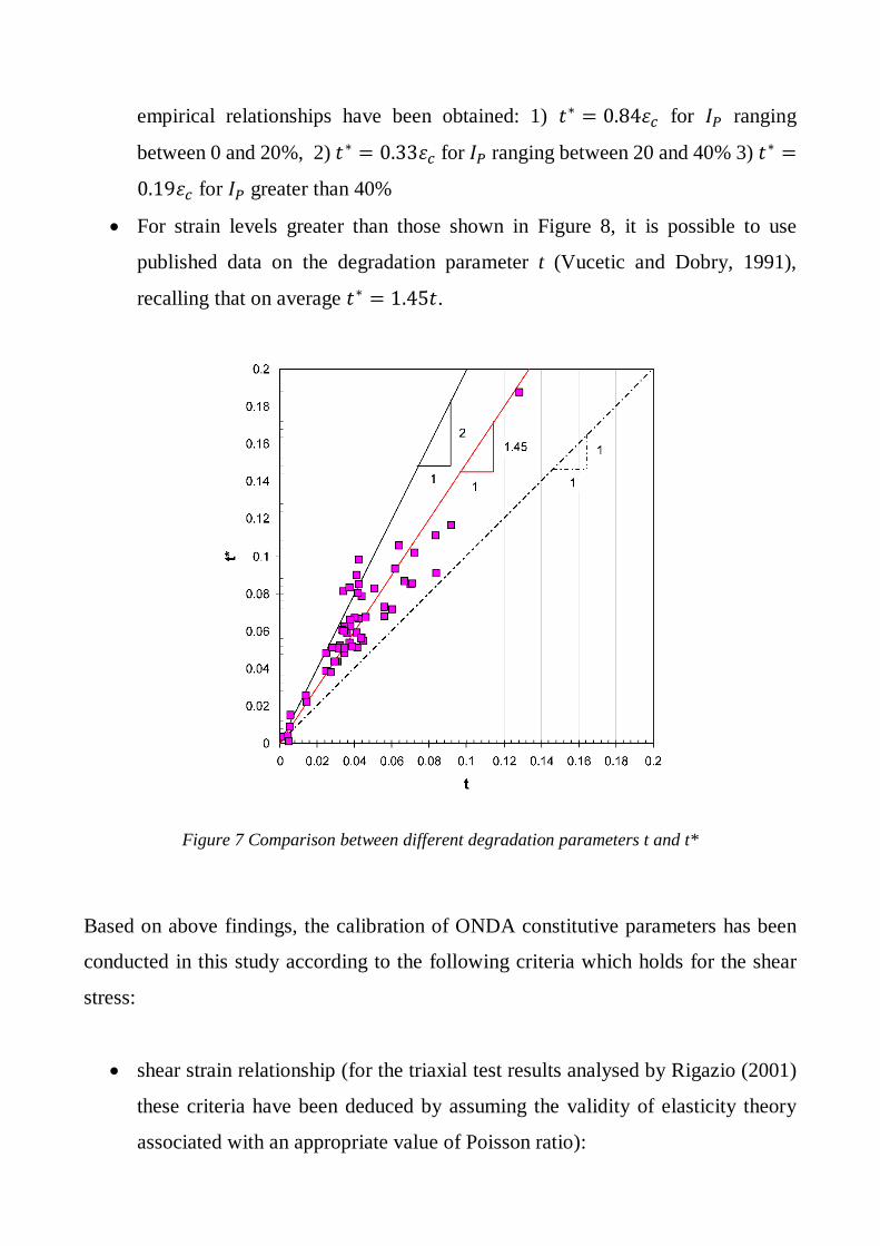
empirical relationships have been obtained: 1) 𝑡𝑡∗ = 0.84𝜀𝜀𝑐𝑐 for 𝐼𝐼𝑃𝑃 ranging

between 0 and 20%, 2) 𝑡𝑡∗ = 0.33𝜀𝜀𝑐𝑐 for 𝐼𝐼𝑃𝑃 ranging between 20 and 40% 3) 𝑡𝑡∗ =

0.19𝜀𝜀𝑐𝑐 for 𝐼𝐼𝑃𝑃 greater than 40%

• For strain levels greater than those shown in Figure 8, it is possible to use

published data on the degradation parameter t (Vucetic and Dobry, 1991),

recalling that on average 𝑡𝑡∗ = 1.45𝑡𝑡.

Figure 7 Comparison between different degradation parameters t and t*

Based on above findings, the calibration of ONDA constitutive parameters has been

conducted in this study according to the following criteria which holds for the shear

stress:

• shear strain relationship (for the triaxial test results analysed by Rigazio (2001)

these criteria have been deduced by assuming the validity of elasticity theory

associated with an appropriate value of Poisson ratio):

• For normally consolidated soils it was assumed 𝑛𝑛0=5 up to shear strain level of

about 0.1%.

• For overconsolidated soils (2 < OCR < 4) it was assumed 𝑛𝑛0=3.5 up to shear

strain level of about 0.1%.

• For a strain level greater than 0.1 % the decrease of 𝑛𝑛0 was assumed according

to the curves illustrated in Figure 5b: curve (1) for NC soils and curve (2) for

OC soils.

• The values of the parameter 𝑡𝑡∗ were obtained from Figure 8, as a function of

strain level and plasticity index (𝑡𝑡∗ = 1.26𝛾𝛾𝑐𝑐 for 𝐼𝐼𝑃𝑃 ranging between 0 and 20%;

𝑡𝑡∗ = 0.49𝛾𝛾𝑐𝑐 for 𝐼𝐼𝑃𝑃 ranging between 20 and 40%, and 𝑡𝑡∗ = 0.29𝛾𝛾𝑐𝑐 for 𝐼𝐼𝑃𝑃 greater

than 40%). For strain levels greater than those reported in Figure 8, were used

data on the degradation parameter t published in the literature (e.g. Vucetic and

Dobry 1991), recalling that 𝑡𝑡∗ = 1.45𝑡𝑡.

Figure 8 Influence of Ip on degradation parameter

In the case of transient loading the degradation is taken into account in agreement

with the suggestions given by Idriss et al. (1978). More specifically:

• changes in 𝛿𝛿 are evaluated between zero crossing (i.e. for every half cycle);

• degradation index is evaluated by means of the following equation (see Figure

9) 𝛿𝛿𝐵𝐵𝐵𝐵 = 𝛿𝛿𝐴𝐴𝐵𝐵 �1 + 12

(𝛿𝛿𝐴𝐴𝐵𝐵)1𝑡𝑡∗�

−𝑡𝑡∗

, where 𝑡𝑡∗ is the degradation parameter for the

strain level 𝛾𝛾𝐴𝐴𝐵𝐵

• both backbone curve and hysteretic curve are degraded; it is assumed that 𝛿𝛿′ =

𝐺𝐺𝑁𝑁 𝐺𝐺1⁄ (i.e. the ratio of the secant stiffness at the Nth cycle to that of the first

cycle) on the purpose of degrading the backbone curve.

Figure 9 Schematic representation of variations of stress and strain with time

PLEASE NOTE:

In the txt file containing the main properties of the soil deposit:

Thick

[m]

Unit W.

[kN/m3]

Vs

[m/s]

G0

[MPa]

Damping D0

[-]

R [-

]

alpha [-

]

Tau Max

[kPa]

OCR

(1)

IP

[%]

Label

[#]

15 19 100 0 0.02 2.05 20.1 0 1 10 1

15 19 400 0 0.02 2.05 20.1 0 2 10 2

0.01 22 1200 0 0.02 0 0 0 2 10 1

Use OCR = 1 if you want to consider 𝑛𝑛0=5 (for normally consolidated soils); OCR =

2 if you want to consider 𝑛𝑛0=3.5 (for overconsolidated soils); OCR = 0 if you want to

use 𝑛𝑛0=2.

5.1.2 Convergence parameters

A delicate aspect regarding all discrete models, particularly in non-linear

dynamics, is the convergence and stability of the solution in relation to refinement of

the discretization scheme. In the Ohsaki’s model this is related to the minimum number

of sublayers in which to subdivide the macro-layers of the soil deposit. Sub-layering

criteria depend on several factors including the number of macro-layers, whether the

variation of mechanical impedance with depth is smooth or rough, the frequency

content of the seismic excitation. According to Ohsaki (1982) the number of

subdivisions 𝑁𝑁𝑠𝑠𝑠𝑠𝑏𝑏 is chosen according to the following conditions (the most

restrictive): 1) 𝑁𝑁𝑠𝑠𝑠𝑠𝑏𝑏 must be such that the periods of vibrations determined by the

algorithm are within a 5% error; 2) 𝑁𝑁𝑠𝑠𝑠𝑠𝑏𝑏 must be such that the response of the system

to a given excitation is computed within a 5% error. Also for ONDA it was adopted

the same convergence criterion. Therefore, while macro-strata depend on the

geotechnical profile and are defined by the user in the input data file (Matdat), the

number of layers in which each macro-stratum is subdivided depends on the above

illustrated convergence criteria. The computation accuracy is also affected by the

following factors:

• Time interval of the input accelerogram;

• Maximum frequency;

Input accelerogram should be filtered to cut-off frequency higher than 25 Hz.

However, no specific procedure is considered in ONDA to filter the input

accelerogram.

The time interval of the input accelerogram (dt) should be small enough to verify

the convergence of the solution. Ohsaki and Sakaguchi (1973) indicate and ideal value

of dt = 0.625 milliseconds. Such a value is much smaller than the typical sampling time

of registered accelerogram (10 ÷ 5 ms). Values of dt = 0.0025 to 0.00125s have been

usually adopted in ONDA. If the adopted dt is still too small, this involves an arbitrary

increase of data points in the original accelerogram.

5.2 Output results

The results of computations are saved as tab delimited txt files in a user-defined

folder, using File Save ONDA results.

A list of saved files and their contents and structure is reported in the following:

• filename_profiles.txt – such a file consists of eight columns:

o column 1: sublayer thickness [m]

o column 2: depth at the middle height of the sublayer [m]

o column 3: vertical effective stress at the middle height of the sublayer

[kPa]

o column 4: peak acceleration of the sublayer in [m/s²]

o column 5: maximum shear stress at the middle height of the sublayer [kPa]

o column 6: peak shear strain at the middle height of the sublayer [-]

o column 7: permanent shear strain at the middle height of the sublayer [-]

o column 8: permanent displacement of the sublayer [cm]

• filename_input_acc_spec_depth_acc.txt - such a file consists of three

columns:

o column 1: time [s];

o column 2: the input accelerogram [m/s²];

o column 3: the accelerogram [m/s²] at the depth specified by the users in

the “ONDA Analysis” Tab at the field “Output-Result Depth”.

• filename_input_acc_fs_spec_depth_acc_fs.txt - such a file consists of four

columns:

o column 1: frequency [Hz] related to the output in column 2;

o column 2: fourier spectrum amplitude of the input accelerogram;

o column 3: frequency [Hz] related to the output in column 4;

o column 4: fourier spectrum amplitude of the accelerogram at the depth

specified by the users in the “ONDA Analysis” Tab at the field “Output-

Result Depth”.

• filename_ strains_time_hist.txt - such a file consists of N+1 columns, where

the number N is equal to the number of sublayers in which the soil has been

discretized by the calculation program:

o column 1: time [s];

o column from 2 to N +1: shear strain time history at the middle height of

the sublayer.

• filename_ stresses_time_hist.txt - such a file consists of N+1 columns:

o column 1: time [s];

o column from 2 to N +1: stress time history at the middle height of the

sublayer.

• filename_ accel_time_hist.txt - such a file consists of N+1 columns:

o column 1: time [s];

o column from 2 to N +1: acceleration time history at the middle height of

the sublayer.

• filename_ displ_time_hist.txt - such a file consists of N+1 columns:

o column 1: time [s];

o column from 2 to N +1: displacement time history at the middle height of

the sublayer.

• filename_ vel_time_hist.txt - such a file consists of N+1 columns:

o column 1: time [s];

o column from 2 to N +1: velocity time history at the middle height of the

sublayer.

• filename_ permanent_displ_profile.txt - such a file consists of 2 columns:

o column 1: permanent displacement at the middle height of each sublayer

[m];

o column 2: depth at the middle height of the sublayer [m]

• filename_ spec_depth_Elastic_Spectrum.txt - such a file consists of 2

columns:

o column 1: Period T [sec];

o column 2: Elastic response spectrum PSA [g] at the depth specified by the

users in the “ONDA Analysis” Tab at the field “Output-Result Depth”.

Additional results can be computed using the Tab “Other Outputs”. In this Tab

it’s possible to calculate and plot: 1) the acceleration time history, 2) the fourier

spectrum and 3) the elastic response spectrum for a specified sublayer number. This

can be done filling the “Number of the layer” field and pushing the Plot button. Then

these outputs can be saved as tab delimited txt files in a user-defined folder, using File

Save Other results.

A list of saved files and their contents and structure is reported in the following:

• filename_acc_other.txt - such a file consists of three columns:

o column 1: time [s];

o column 2: the input accelerogram [m/s²];

o column 3: the accelerogram [m/s²] at the sublayer number specified by the

user in the “Other Outputs” Tab.

• filename_ acc_fs_other.txt - such a file consists of four columns:

o column 1: frequency [Hz] related to the output in column 2;

o column 2: fourier spectrum amplitude of the input accelerogram;

o column 3: frequency [Hz] related to the output in column 4;

o column 4: fourier spectrum amplitude of the accelerogram at the sublayer

number specified by the user in the “Other Outputs” Tab.

• filename_Elastic_Spectrum_other.txt - such a file consists of 2 columns:

o column 1: Period T [sec];

o column 2: Elastic response spectrum PSA [g] at the sublayer number

specified by the user in the “Other Outputs” Tab.

The following plots are given:

• “Accelerogram” Tab: input accelerogram and that at the depth specified by the

users in the “ONDA Analysis” Tab at the field “Output-Result Depth”.

• “Fourier spectrum” Tab: Fourier spectra of the input accelerogram and that at

the depth specified by the users in the “ONDA Analysis” Tab at the field

“Output-Result Depth”;

• “Elastic R-Spectrum” Tab: elastic response spectrum of SDOF at the depth

specified by the users in the “ONDA Analysis” Tab at the field “Output-Result

Depth”;

• shear strain time history at the selected layers;

• “Strain Displ Time-History” Tab: Strain and displacement time histories at

the selected sublayer;

• “Peak Profiles” Tab: maximum acceleration and shear strain profiles;

• “Stress-Strain” Tab: stress-strain time histories at the sublayer specified and at

the following 3 sublayers;

• “Permanent displ” Tab: permanent displacement profile;

• “Other Outputs” Tab: acceleration time history, fourier spectrum and elastic

response spectrum at the specified sublayer number.

It’s possible to re-load saved results using View ”Load….” and plot these results

using the “Plot ….Viewer” buttons in the plotting Tabs.

REFERENCES Bardet, J.P., Ichii, K. and Lin C.H. (2000). “EERA – A Computer Program for Equivalent- Linear Earthquake Site Response Analyses of Layered Soil Deposits.”, Department of Civil Engineering, University of Southern California, http://geoinfo.usc.edu/gees. Bardet J.P. and Tobita T. (2001). “NERA: Nonlinear Earthquake Site Response Analysis of Layered Soil Deposits”, University of California, http://geoinfo.usc.edu/gees. Camelliti, A. (1999). Influenza dei Parametri del Terreno sulla Risposta Sismica dei Depositi. M.Sc. Thesis, Dipartimento di Ingegneria Strutturale e Geotecnica, Politecnico di Torino, Italy, December, pp. 125 (in Italian). Chopra, A.K. (1995). “Dynamics of Structures .”, Prentice-Hall. Constantopoulos I.V., Roësset J.M. and Christian J.T. (1973). “A Comparison of Linear and Exact Nonlinear Analysis of Soil Amplification.” 5th WCEE, Roma 1973, pp: 1806- 1815. De Martini-Ugolotti P. (2001). Evaluation of the Seismic Response at Castelnuovo di Garfagnana (Italy) by Means of Different Methods of Analysis. M.Sc. Thesis, Imperial College, London. Idriss I.M., Dobry R. and Singh R.D. (1978), “Non linear behaviour of soft clays during cyclic loading”, Journal of the Geotechnical Engineering Division, Proc. ASCE, No. GT12. Idriss, I.M., and Sun, J.I. (1991). “SHAKE91: A Computer Program for Conducting Equivalent Linear Seismic Response Analyses of Horizontally Layered Soil Deposits.”, Program Modified based on the Original SHAKE program published in December 1972 by Schnabel, Lysmer & Seed, Center for Geotechnical Modeling, Department of Civil and Environmental Engineering, University of California, Davis. Ionescu F. (1999) Caratteristiche di deformabilità di sabbie silicee da prove torsionali cicliche e monotone. Ph. D. Thesis, Politecnico di Torino, Department of Structural and Geotechnical Engineering (in Italian). Ishihara, K. (1996). “Soil Behaviour in Earthquake Geotechnics.”, Oxford Science Publications, Oxford, UK, pp. 350. Iwan W.D. (1967). “On a Class of Models for the Yielding Behaviour of Continuous and Composite Systems”. Journal of Applied Mechanics. Vol. 34: 612-617. Joyner, W.B. and Chen, A.F.T. (1975). “Calculation of Non-Linear Ground Response in Earthquakes”, Bulletin of Seismological Society of America, Vol. 65, No. 5, pp. 1315- 1336. Kramer, S.L. (1996). “Geotechnical Earthquake Engineering.”, Prentice-Hall, New Jersey, pp.653. Lee, M.K. and Finn, W.L.L. (1978). “DESRA 2C – Dynamic Effective Stress Response Analysis of Soil Deposits with Energy Transmitting Boundary Including Assessment of Liquefaction Potential.”, Soil Mechanics Series No. 38. Department of Civil Engineering, University of British Columbia, Vancouver, Canada.

Lo Presti D.C.F., Pallara O., Cavallaro A. and Maugeri M. (1998). “Non Linear Stress- Strain Relations of Soils for Cyclic Loading.”, Proceedings of the 11th European Conference on Earthquake Engineering, 6-11 September 1998, Paris, Balkema, pp.187. Lo Presti D.C.F., Pallara O, Cavallaro A. & Jamiolkowski M. 1999 Influence of Reconsolidation Techniques and Strain Rate on the Stiffness of Undisturbed Clays from triaxial Tests. Geotechnical Testing Journal, 22(3): 211-225. Lo Presti D.C.F., Cavallaro A., Maugeri M, Pallara O and Ionescu F. (2000). “Modelling of Hardening and Degradation Behaviour of Clays and Sands During Cyclic Loading.” 12th WCEE, Auckland 30 Jan. to 4 Feb. 2000, paper No. 1849/5/A. Lo Presti D.C.F. & Pallara O. 2003 Stiffness and Damping Parameters For 1D Non-Linear Seismic Response Analysis. Submitted for possible publication to IS Lyon 03. Lo Presti D.C.F., Lai C.G., Puci I. (2003). ONDA (One-dimensional Non-linear Dynamic Analyses): A Computer Code for Non-Linear Seismic Response Analyses of Soil Deposits. Submitted for possible publication to the Journal of Geotechnical and Geoenvironmental Engineering. Lo Presti D.C.F., Lai C.G., Pallara O., Puci I. and Saviolo A. (May, 2003). ONDA (One-dimensional Non-linear Dynamic Analyses): A Computer Code for Non-Linear Seismic Response Analyses of Soil Deposits. User’s Manual version 1.3. Politecnico di Torino, Department of Structural and Geotechnical Engineering. Lubliner, J. (1990). “Plasticity Theory.”, Macmillan Publishing Company, New York, pp.495. Masing G. (1926). “Eigenspannungen und Verfestigung Beim Messing” Proc. 2nd International Congress of Applied Mechanics, Zurich, Swisse. (in German). Matasovic, N., (1993) – Seismic Response of Composite Horizontally-Layered Soil Deposits. Ph.D. Thesis, Civ. Eng. Dep. , School of Eng. And Applied Science, University of California, Los Angeles. Ohsaki Y. (1982) Dynamic Non Linear Model and One-Dimensional Non Linear Response of Soil Deposits, Department of Architecture, Faculty of Engineering, University of Tokyo, Research Report 82-02. Ohsaki Y. & Sakaguchi O. 1973 Major Types of Soil Deposits in Urban Areas in Japan. Soils & Foundations, Vol. 113, No. 2. Pyke, R.M. (1979). “Non-linear soil models for irregular loadings”. Proc. ASCE, Journal of the Geotechnical Engineering Division, Vol. 105, No. GT6, pp: 715-726. Ramberg W. and Osgood W.R. (1943). “Description of Stress-Strain Curves by Three Parameters.” Technical Note 902, National Advisory Committee for Aeronautics, Washington DC. Rigazio A. (2001). Parametri di Rigidezza e Smorzamento per l’Analisi Semplificata della Risposta Sismica di Dighe in Terra. M. Sc. Thesis, Dipartimento di Ingegneria Strutturale e Geotecnica, Politecnico di Torino, pp. 137 (in Italian).

Saviolo A. (2002). Valutazione Effetti di Non-Linearità nella Risposta Sismica dei Terreni con ONDA. M.Sc. Thesis, Dipartimento di Ingegneria Strutturale e Geotecnica, Politecnico di Torino. In-progress (in Italian). Schnabel, P.B., Lysmer, J., and Seed, H.B. (1972). “SHAKE: a Computer Program for Earthquake Response Analysis of Horizontally Layered Sites”, Report EERC 72-12, Earthquake Engineering Research Center, University of California, Berkeley. Streeter V.L., Wylie E.B., Benjamin E. and Richart F.E. JR. (1974). “CHARSOIL - Soil Motion Computations by Characteristics Method.” Journal of Geotechnical Engineering Division, ASCE, Vol. 100, No. GT3, pp. 247-263. Tatsuoka, F. and Shibuya, S. (1992), “Deformation Characteristics of Soil and Rocks from Field and Laboratory Tests,” Keynote Lecture, IX Asian Conference on SMFE, Bangkok, 1991, vol. 2, pp. 101-190. Tatsuoka F., Siddique M.S.A., Park C-S, Sakamoto M. and Abe F. (1993), “ Modeling stress-strain relations of sand”, Soils and Foundations, 33(2), 60-81. Vercellotti L. (2001). Analisi Sismica di Dighe in Terra: Metodi Semplificati. M.Sc. Thesis, Dipartimento di Ingegneria Strutturale e Geotecnica, Politecnico di Torino, pp. 125 (in Italian). Vucetic M. and Dobry R. (1991). “Relation Between the Basic Soil Properties and Seismic Response of Natural Soil Deposits”. International Symposium on Building Technology and Earthquake Hazard Mitigation. Kunming, China. Vucetic, M. (1994). “Cyclic Threshold Shear Strains in Soils.”, Journal of Geotechnical Engineering, ASCE, Vol.120, No.12, pp.2208-2228.