On the verification of a potential based low order ... · order boundary element method for On the verification of a potential based low Portugal ... Bernoulli’s equation,

incompressible flowsorder boundary element method forOn the verification of a potential based low

PortugalDepartment of Mechanical Engineering, h t i t u t o Superior Te'cnico,G.B. Vaz, L. E g a 8~J.A.C. FalcZo de Campos

Abstract

the calculation to zero element size.derive the apparent order of accuracy and to perform the extrapolation ofin series of geometrically similar grids appears to be a viable approach toA verificationprocedure based on a least-squares fit of the numerical resultsand non-lifting 2-D and 3-D flows by comparison with analytical solutions.error behavior when decreasing the typical element size in lifting 2-D flowsFor a low-order potential based boundary element method we examine the

1 Introduction

relatively small computational expenses.ement method is able to deal with complex geometric configurations atnumber attached flows to engineering accuracy and that the boundary el-distributions are predicted by the potential flow model in high Reynoldsfiguration. This is a consequenceof the fact that lift forces and foil pressurenique to compute relevant aero or hydrodynamic characteristics of the con-with the boundary element method (or panel method) is an efficient tech-tions with lift, the simple incompressible inviscid potential flow analysisIn many hydrodynamic and low-speed aerodynamic flows past configura-

a body. This results in a Fredholm integral equation of the second kind forapplies a Dirichlet boundary condition for the perturbation potential insidemethod, [3]. This method is based on Green's theorem for the potential and[ 2 ] . A rather popular method is the low-order potential based Morino paneldifferent types of applications, see for reviews Hess [l]and Hoeijmakers

Various types of panel or boundary element methods are in use for

© 2002 WIT Press, Ashurst Lodge, Southampton, SO40 7AA, UK. All rights reserved.Web: www.witpress.com Email [email protected] from: Boundary Elements XXIV, CA Brebbia, A Tadeu and V Popov (Editors).ISBN 1-85312-914-3

be more accurate for thin foils, [4].CPU memory requirements than velocity based methods and is known to(hyperboloidal) elements. This method is simple to implement, it has lowerorder version it uses constant dipole and source distributions on bi-linearfrom the Neumann boundary condition on the body surface. In the lowthe surface potential since the surface source distribution becomes known

estimates for the extrapolated value may be derived, [6].order of accuracy of the method. Also, from the error behavior, uncertaintycreasing grid size follows a power law, whose exponent is related to thenumber). It is usually assumed that the asymptotic error behavior for de-to zero grid size (or in the boundary element method for infinite elementobserved error behavior with grid size, to determine an extrapolated valuenumerical calculations for a sequence of grids and, from an assumed or the[5], AIAA [6]. In general terms, it would simply consist in performing therequirement is to perform verificationof the numerical calculations, Roachedo not exceed those errors. The recommended procedure to satisfy suchadopted flow model, but it is essential to require that the numerical errorscal errors to levels substantially lower than the errors associated with thethe numerical error in the prediction. It is useless to reduce the numeri-to predict the characteristics of a configuration, it is important to quantify

In a practical situation, when the boundary element method is applied

to more practical cases, such as the Joukowski foil or the thin ellipsoid.cylinder or the sphere, to less well behaved solutions that bear resemblanceflows. These cases range from well-behaved solutions, such as the circulara sphere and a thin ellipsoid with three unequal axis in three-dimensionalcircular cylinder, Joukowski foils at incidence in two-dimensionalflows; andmethod for decreasing element size. The analytical solutions chosen are acalculations performed with a low-order potential based boundary elementThe purpose of this paper is to examine the error behavior of numericalits asymptotic behavior may be established for grid size approaching zero.is performed against analytical solutions, the error can be evaluated andthe grid size approaches zero. Prior to this, and when code verificationerror estimation [6], strongly hinges on the asymptotic error behavior when

It is clear that the verificationof numerical calculations, which involves

2 BEM Formulation

2.1 Mathematical model

outer control surface S, surrounding the body and wake surface. A unitsurface Sa, a wake surface SW trailing from the foil trailing edge, and theboundary S , as pictured in Fig.1. The boundary S is composed of the bodyflow. Consider a general two or three dimensional fluid flow domain V withnamic configurationis a potential flow model for inviscidand incompressibleThe model adopted to describe the flow field around a hydro or aerody-


vector 5 normal to S is defined oriented into the domain V, Fig.1.

Figure l: Geometry domain and notation for the potential flow problem.

denote the potential on the upper and lower sides at the trailing edge.the circulation around the foil: ( L I $ ) , , ~ = $+ - q5-, where q5+ and $-the Kutta condition at the trailing edge is required to uniquely determine[7].In the two-dimensional case, where the domain is multiply connected,wake surface, but its discussion isbeyond the scope of this paper, see [2] andkinematic and dynamic boundary conditions have to be imposed on thediscontinuity of the potential across SW. In the three-dimensional case,vanishes V$ + 0, as S, + m. In the lifting problem we allow for aSa and, on the outer control surface, the flow disturbance due to the bodyThe kinematic boundary condition 2 = -cw.f i is satisfied on the surfacebody. The perturbation potential satisfies the Laplace equation V2$= 0.c&,= Vq5&,,and q5 is the perturbation potential due to the presence of thepotential @ = +&,+ $, where &, is the potential of the undisturbed flow,function @ related to the flow velocity by = V@. We write for theV the flow is assumed irrotational so that we may introduce a potentialof a foil placed in a uniform onset flow with velocity c&,.In the domain

For the purposes of this study we restrict ourselves to the steady case

domain is,V', +' = 0, the integral representation of the potential at a point p in the

By application of Green's theorem, assuming for the interior domain

if p E Sa,Sw.tween the points p and q , and E (p) = 1 if p is interior to V, or E (p) = l / 2(1/27r) logR (p,q ) in the two-dimensional case, R (p,q ) is the distance be-where G (p,q) = -l/ (47rR(p,q)) in the three-dimensionalcase and G (p,q ) =


1 6 B o u ~ i w - ~ ~E l m c n t s X X I V

Kutta condition.tential discontinuity A4 (Q) is related to the surface potential through thekind on the unknown body surface potential 4 ( q ) . The wake surface po-the body surface Sa, Eq.(l) is a Fredholm integral equation of the second

With the on SBknown from the Neumann boundary condition on

2.2 Numerical implementation

see, for instance, Katz and Plotkin [4].The matrix coefficientsor influence coefficientsare determined analytically,the collocation method with the element center point as collocation point.coincidentwith the singular point. The integral equation Eq.(l) is solved byelements. At grid singularities, triangular elements are used with one nodements are straight elements and in three-dimensions bi-linear quadrilateraltial and source distributions on each element. In two-dimensions the ele-The boundary element method used in this work assumes constant poten-

Vaz et a1 [8]. Here we use the simple Morino Kutta condition, given in 2.1.dition have been used. Their effect on the solution has been discussed in

In the case of a lifting foil, various implementations of the Kutta con-

Bernoulli’s equation, the pressure coefficient C, can be determined fromof the potential relative to the arc lengths on the body surface grid. Fromcomponentsare calculated by means of a second order differentiationschemeFrom the potential solution on the surface the covariant surface velocity

The resulting matrix equation is solved by a LU factorization method.

c, = 1- (g)2.3 Verification Procedure

the following power series expansionis assumed that the error of a numerical calculation may be represented byIn any of the existing verification procedures available in the literature, i t

contribution of all the other terms, then Eq.(2) becomes :i.e. the contribution of the leading term of the series is larger than thetypical element size. If we assume that a grid is in the asymptotic range,in a grid of typical size hi. In boundary element methods, it represents thewhere p i is the numerical solution of a given flow quantity, local or integral,

to the Richardson extrapolation of the numerical solution, where p. standswherep is the apparent order of accuracy of the method. Eq.(3) corresponds

e ( p i ) = pi - p. = ah:, (3)


solution, pe.for the solution in a grid of size zero, which should be equal to the exact

in more than three grids.squares root approach suggested in [g], which requires numerical solutionsof po, Q and p. Therefore, in the present study we have adopted the least-the results obtained from different grid triplets may lead to different setsto guarantee that all the grids are in the asymptotic range. Furthermore,reported in [g] show that from the practical point of view it may be difficultis required to confirm that Eq.(3) is satisfied. The verification exercisessolutions are required to obtain p o , a and p. At least a fourth solution

If the order of accuracy p is not assumed to be known, three numerical

function :In this approach, po, a and p are obtained from the minimum of the

no

S ( P w %P) = 4 g ( P i - ( P o + ah:))2, (4)

where ng is the number of grids.

4 Results and Discussion

4.1 Two-Dimensional flows

full cosine function of the coordinate along the chord.1000. In all grids the element corner point distribution is obtained from aa series of 15 geometrically similar grids, with element numbers from 20 toCalculations were performed for the circular cylinder and Joukowskifoils in

the normal to the element intersects the exact surface.points. These are obtained using the analytical value at the point whereL, and L a , were obtained from numerical solution errors at the collocationas function of the arc length are used for the interpolation. Error norms,higher than the order of discretization errors, cubic splines of the solutionsolution at collocation points. To keep the order of the interpolation errorsfrom the analytical solution using interpolated values from the numerical

The local solution error values of potential and pressure were evaluated

The coincidence of p for the two error norms and the two local quantitiesbecause the same values of p and a are obtained for different sets of grids.that the results obtained in the finest grids are in the asymptotic range,potential at the two locations and for the L, and L 2 norms. It is clearresults show that an apparent order of accuracy of 2 is obtained for thebetween the two number of elements given in each row of the tables. Thepresent the correspondingverification results for the sets of grids comprisedaligned with the x axis and the flow is without circulation. Tabs.1 and 2norms of the potential and pressure coefficient. The uniform onset flow iserrors at two different locations on the circular cylinder and of the error

Figs.2(left) and 2(right) show,respectively,the convergenceof the local


1 8 B o u ~ i w - ~ ~E l m c n t s X X I V

velocity calculation is second order accurate.potential. However, for this particular solution it is easily seen that thethat it obtained from velocities, which are derived by differentiation of thethe pressure coefficient is also second order convergent, despite the factis a linear function of the z coordinate. It is interesting to observe thattheoretical first order, for this particular simple solution, since the potentialaccuracy in all the cylinder. The second order convergence ishigher than theindicate that we have a "well-behaved" solution with the same order of

l d ld I dN

(right)-Error norms of potential and pressure coefficient on a cylinder.on a cylinder. LOCI(: = 0.96,f = -0.19), LOCZ($ = 0.50, = -0.50).Figure 2: (left)-Local solution errors of potential and pressure coefficient

norms are not adequate to extrapolate local quantities.the assumed behavior of the error. However, the values of p for the errorthe error of the local solutions, the error norms present an acceptable fit tothe error for this range of grids. Although we have a different behavior ofedge the solution convergesbut it does not match the assumed behavior oflocation exhibits a value of p of 1.5 and at the location close to the leadingfirst location and 1.4 for the second. The pressure coefficient at the secondpotential has different values of p in the two selected locations: 1.9 for thecylinder. The values of p are sensitive to the sets of grids selected. Theon the upper side. In this case the scenario is more complex than for theare a point close to the leading edge, LOCI,and a point at mid-chord, LOQ,4 present the corresponding verificationresults. The two selected locationsaround the circular cylinder with circulation, Batchelor, [lo]. Tabs.3 andattack. The analyticalsolution is obtained by conformalmapping of the flowfoil with maximum thickness to chord ratio t / c = 0.04 at a = 2" of angle of

Figs.S(left) and S(right) show similar results for a symmetric Joukowski

mid-point rule, C l p . Tab.5 presents the verification results. The apparentKutta-Joukowski law, C l J , or direct numerical pressure integration withresults for the lift coefficient on the symmetric Joukowski foil calculated byphysical interest, such as the lift coefficientof the foil. Fig4(left) showssuch

It is interesting to examine the convergenceof an integrated quantity of


B o u d u r - y E k w w ~ t sX X I V 1 9

Table 1: Verification results for local solution errors on a cylinder.

Grids

1000-1001000-1501000-2001000-3001000-4001000-5001000-6001000-7001000-800

e

2.00 -0.304 2.0010.0

p 1 X 104a x 108e C P L o c , e l,0c 2

P

2.00 1 -0.318 2.00-0.5002.00 -0.318 2.00

-0.500 2.00 -0.318 2.00-0.500 2.00 -0.318 2.00-0.500 2.00 -0.318 2.00-0.500 2.00 -0.318 2.00-0.500 2.00 -0.318 2.00-0.500 2.00 -0.318 2.00

-0.500

-0.500 I( 2.00 I -0.308 / / 2.00

Table 2: Verification results for error norms on a cylinder.

Grids

1000-1001000-1501000-2001000-3001000-4001000-5001000-6001000-70010004300

p 1 a x l o b p 1 a x l o bp 1 a x lob

L - ( e 4 1 L Z e c p L OL 2 ( e + )h 1!!i

P

2.00 1 0.581 2.00 1 0.822 2.03 1 0.814 2.001.252.00 0.581 2.00

1.67 2.00 0.581 2.002.00 2.00 0.581 2.002.50 2.00 0.582 2.003.33 2.00 0.582 2.005.00 2.00 0.583 2.006.67 2.00 0.583 2.0010.0 1.99 0.585 1.99

1.43 2.03 0.813 2.000.822 2.03 0.812 2.000.822 2.03 0.810 2.000.823 2.04 0.806 2.000.823 2.05 0.799 2.000.824 2.06 0.784 2.000.825 2.08 0.766 2.000.828 2.10 0.730 2.00

0.822

l@

I O 2

-1 0 ~ ~

Ls

Id

10.'

10"

ld ldN

%%F

0.1320.1320.1320.1320.1320.1320.1320.1320.132

xa x 10

0.261

0.2600.2610.2610.2610.2610.2610.2610.261

coefficient on the symmetric Joukowski foil.L O C ~(: = 0.50,$ = 0.015). (right)-Error norms of potential and pressurecient on the symmetric Joukowski foil. LOCI(T = 0.00075, $ = 0.0017),Figure 3: (left)-Local solution errors of potential and pressure coeffi-

extrapolated with the complete set of grids with different apparent orders300- 1000lead to a 5 digit accurate extrapolated value. However, the valuesquare fits obtained for C l J using grids 800 - 1000 and C l p using gridsorder of accuracy is dependent on the set of grids selected. The least-


20 B o u ~ i w - ~ ~E l m c n t s X X I V

used than the apparent order of accuracy.shows that the extrapolated value is less sensitive to the number of gridsof accuracy (1.13 for C l J and 1.26 for C l p ) is already 4 digit accurate. This

Joukowski foil.Table 3: Verification results for local solution errors on the symmetric

Grids 1 2 I k1000-800 1 1.25 1 1 1.93

1000-1001000-1501000-2001000-3001000-4001000-5001000-6001000-700

1.983.33 2.005.00 2.016.67 1.95

1.941.67 1.952.00 1.972.50

1.43

10.0 1 1 1.53

&0.223 1 1 1.37

1.340.211 1.310.208 1.270.228 1.24

1.370.220 1.360.218 1.350.215

0.222

0.499 1 1 1.16

zz+0.155 1 1 3.43

2.720.166 2.510.176 4.650.188 2.76

3.180.157 2.980.159 2.820.161

0.156

0.220 1 1 2.95L 0.258 1 1 1.410.364 1.430.019 1.450.255 1.460.208 1.460.193 1.470.174 1.470.156 1.47

0.460

0.5090.4830.4740.466

1

Table 4: Verification results for error norms on the symmetric Joukowskifoil.

1000-1001000-1501000-2001000-3001000-4001000-5001000-6001000-700

2.00

3.330.1880.185

0.221

a x 10

7a X 104 1 1 p

0.295 1 1 2.110.296 2.100.299 2.090.302 2.070.307 2.050.316 2.030.335 2.140.357 2.200.412 1.94

7Ta x 10

0.1460.0890.0980.1130.1120.1090.1080.1070.106

0.135

0.155

C l J

foil. Exact C l , pe = 0.226033770.Table 5: Verification results for C l J and C l p on the symmetric Joukowski

C l p2Grids a x IOdp P O a x 106p P O

-0.121 0.226041100 1.37 -0.124 0.2260386831000-400 2.50 1.30 -0.123 0.226043326 1.36 -0.125 0.2260401061000-300 3.33 1.28 -0.126 0.226047338 1.35 -0.128 0.2260426191000-200 5.00 1.24 -0.134 0.226056295 1.32 -0.132 0.2260480731000-150 6.67 1.20 -0.143 0.226067193 1.30 -0.138 0.2260546411000-100 10.0 1.13 -0.167 0.226096022 1.26 -0.150 0.226070923

1.25 1.35 -0.118 0.226038126 1.39 -0.122 0.2260367621000-700 1.43 1.34 -0.118 0.226038763 1.39 -0.123 0.2260371661000-600 1.67 1.33 -0.119 0.226039696 1.38 -0.123 0.2260377711000-500 2.00 1.32

1000-800

ues of the lift coefficient as function of the number of elements for a 10%Fig.C(right) depicts the difference betweenthe numerical and analytical val-

As an illustration of the possible error behavior of the lift coefficient,


10' l d I dN

Joukowski foil, t / c = 0.10.Joukowski foil, t / c = 0.04. (right)-Error of lift coefficient vs camber for theFigure 4: (left)-Verification results for lift coefficients on the symmetric

based on the coarsest grids will "miss" the analytical value, as seen in [8].a maximum value and decreasing to zero. In such cases the extrapolationcertain number of elements where the error crosses zero before increasing tois monotone, but for increasing camber it is not. For each camber there is aelements has been used. For zero camber (symmetric foil) the convergencethick Joukowski foil with various cambers. A maximum number of 2000

4.2 Three-dimensionalFlows

stretching functions along the x and y coordinates are used.ellipsoid section y = const. and the second the number of sections. Cosine256 x 128-G5, where the first figure denotes the number of elements on thegrids is used: 16 x 8 -Gl , 32 x 16-G2, 64 X 32 -G3, 128 x 64-G4 andsphere and ellipsoid are shown in Fig.5. A series of 5 geometrically similaraxis. The ellipsoid results are taken from [ll].The surface grids on thewith a = 1, b = 2, c = 0.1 in a uniform onset flow aligned with the xResults are presented for a sphere and an ellipsoid ( z ) + (b) + ( z ) ' = 1

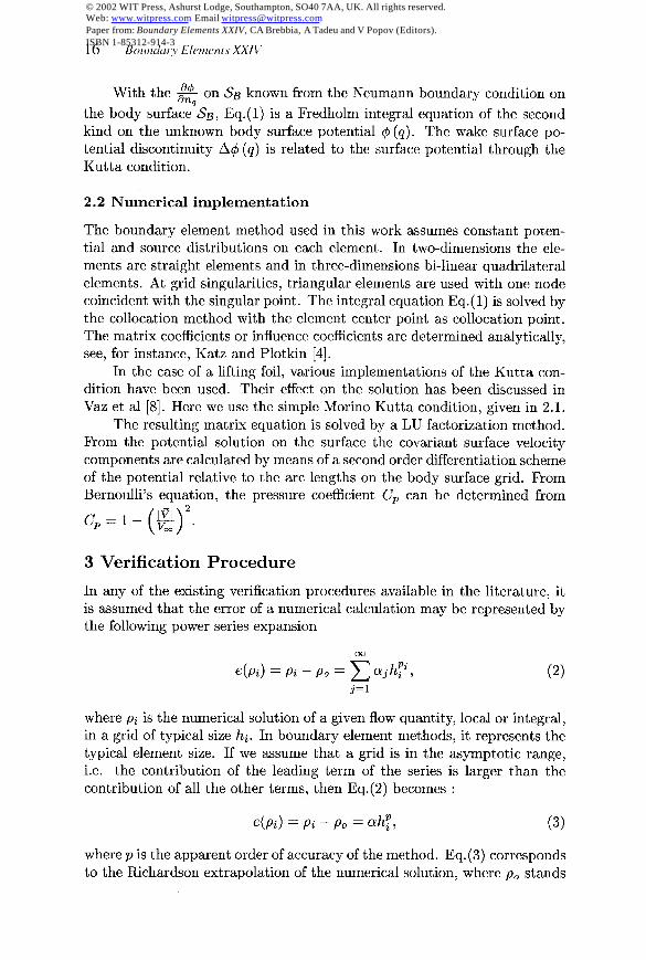
is further reduced in comparison with the sphere case. The pressure coef-close to the grid singularity, the apparent order of accuracy of the potentialcase discretizedwith the present grid types, which are highly non-orthogonalthe maximum error is being shifted when refining the grid. For the ellipsoidror norms no reasonable least-squares fit can be obtained, as the position ofThe pressure coefficient convergence is considerably lower. For the L, er-function of x and, therefore, near second order convergence is expected.for the two norms. Also, for this simple test case, the potential is a linearof the sphere, the apparent order of accuracy of the potential is close to 27 present the correspondingverification results. In the "well-behaved" casetential and pressure coefficient on the sphere and the ellipsoid. Tabs.6 and

Fig.6 show the convergence of the error norms L, and L 2 of the po-


Figure 5: Grids on the sphere and ellipsoid.

may be derived from the error norms.ficient appears to converge in this case but no reasonable least-squares fit

1 1N I n

EeW

J

ellipsoid, [1l].sphere. (right)-Error norms of potential and pressure coefficient on theFigure 6: (left)-Error norms of potential and pressure coefficient on a

5 Conclusion

ary element method. Furthermore, the use of a verificationprocedure baseding two-dimensionalflow past foils with a low-order potential based bound-Laplace equation in non-lifting two and three-dimensional flows and in lift-ment approaching zero. We examined the error behavior of the solutions ofthe discretized equations approach the continuum solution for grid size ele-ification against analytical solutions is required to check if the solution ofbuild confidence in computational codes. Prior to such exercises, code ver-Verification of numerical calculations is becoming a mandatory exercise to

J


B o u d u r - y Elpnwnts X X I V 23

Table 6: Verification results for error norms on a sphere.

X 104 p a X 103 p a x loLp

L- ( e 4 1 ~2 ( . cp) L , ( . c p )L 2 ( G P )% p x 104

G r i d s

1.98 0.15 1.95 0.33 1.44 0.55 0.92 0.75G5-G2 4.0 1.95 0.16 1.91 0.35 1.56 0.46 0.87 0.84G5-G1 8.0 1.86 0.20 1.78 0.46 1.88 0.23 1.42 0.23

2.0G5-G3

Table 7: Verification results for error norms on the ellipsoid.

X 104 p a x 103 p a x loLpL- ( e + ) ~2 (ec,) L , (.cp)L:! ( e 4 1

% p (y xG r i d s

1.52 0.14 1.02 0.90 2.16 0.78 1.13 1.23G5-G2 4.0 1.64 0.12 1.66 0.31 2.26 0.67 2.20 0.23G5-G1 8.0 1.72 0.10 1.41 0.52 0.60 25.6 0.16 41.6

2.0G5-G3

investigated.on a least-squares fit of the numerical results on sequences of grids has been

extrapolations to zero element size.results on at least three grids appears to be a viable approach to performThe verification procedure based on the least-squares fit of the numericalfor each relevant quantity from the results on the successively refined grids.or the 3-D ellipsoid case), the apparent order of accuracy has to be found"well-behaved" practical cases (illustrated here by the 2-D Joukowski foilflow domain is already in the asymptotic range of the grids used. In lessder of accuracy of the method in "well-behaved" problems where the wholederived quantities. Error norms are only representative of the apparent or-perform extrapolations to zero element size of local or global, primitive or

Theoretical orders of accuracy of the method can not be relied upon to

Acknowledgments

discussions on this topic.authors are indebted to Mr. Johan Bosschers of MARIN for many usefulThis work was done under the project PRAXIS/2/2.1/MAR/1723/95.Thepara a Ciikcia e a Tecnologia, Ph.D. grant PRAXISXXI/BD/22269/9.The first author acknowledgesthe financial support granted by Funda$%o

References

P I

P I

P I

1974.configurations: a general theory, AIAA Journd, 12(2), pp.191-197,Morino, L. & Kuo, C.C., Subsonicpotential aerodynamics for complexdesign, AGARD Report 783, January 1992.Hoeijmakers, H.W.M., Panel methods for aerodynamic analysis andReview Fluid Mechanics, 2 2 , pp.255-274, 1990.Hess, J.L., Panel methods in computational fluid dynamics, Annual


24 B O L M ~ ~ I - J ~Elcmcnts X X I V

panel methods, McGraw-Hill, 1991.[4]Katz, J., Plotkin, A., Low-speed Aerodynamics. From wing theory to

[6] American Institute for Aerodynamics and Astronautics, Guide forand Engineering, Hermosa publishers, Albuquerque, USA, 1998.

[5] Roache, P. J., Verification and Validation in Computational Science

da t ions , AIAA-G-077-1998, 1998.Verification and Validation of Computational Fluid Dynamics Sim-

CRC, 95, pp.240-251, 2000.equation; trailing-edge conditions in aerodynamics, Chapman & Hall-

[7]Morino,L., Bernardini, G., Singularities in discretizedBIEs for Laplace’s

of steady 2D flow around foils, Proc. of B E M 22, Cambridge, 2000.locity and potential based boundary element methods for the analysis

[8] Vaz, G.B., Eqa, L., Falciio de Campos, J.A.C., A comparison of ve-

1999.Flow Calculations, Proc. of 1s t MARNET-CFD Workshop , Barcelona,

[g] Eqa, L. & Hoekstra, M., On the numerical verification of Ship Stern

versity Press, 1967.[lo] Batchelor, G., An Introduction to Fluid Dynamics, Cambrigde Uni-

panel codes, submitted for publication in Computers and Fluids.A verification study on low-order three-dimensional potential based

[ll]Falciio de Campos, J.A.C, Ferreira de Soma, P.J.A., Bosschers, J.,


Documents

On the verification of a potential based low order ... · order boundary element method for On the verification of a potential based low Portugal ... Bernoulli’s equation,