ON THE

VALUATION OF

CORPORATE BONDS USING

RATING-BASED MODELS

by

Edwin J. Elton,* Martin J. Gruber,*

Deepak Agrawal** and Christopher Mann***

September 15, 2003

* Nomura Professors, New York University

** KMV Corporation

*** Moodys

1

The valuation of corporate debt is an important issue in asset pricing. While there has

been an enormous amount of theoretical modeling of corporate bond prices, there has been

relatively little empirical testing of these models. Recently there has been extensive development

of rating based models as a type of reduced for model. These models take as a premise that

groups of bonds can be identified which are homogeneous with respect to risk. For each risk

group the models require estimates of several characteristics such as the spot yield curve, the

default probabilities and the recovery rate. These estimates are then used to compute the

theoretical price for each bond in the group. The purpose of this article is to examine the two

reduced form models that are most widely used and from which most other models are derived

(Duffie and Singleton (1997) and Jarrow, Lando and Turnbull (1997)). We will clarify some of

the theoretical differences between these models and examine how well they explain prices.

The paper is divided into four sections. In the first section we review the various models

for pricing corporate bonds. In the second section we explore the valuation of zero coupon

bonds. We show that for zeros, Duffie Singleton (1997) (hereafter DS) and Jarrow, Lando and

Turnbull (1997) (hereafter JLT) produce the same valuation. In the third section, we show that

these models produce very different results for coupon paying bonds, and that the differences are

functions of coupon and maturity. Finally, in the last section we compare the pricing of the two

models using a large sample of corporate bonds and both show that the differences predicted on

the basis of theory in the prior section hold and measure the magnitudes of the effects.

I. Alternative Models:

There are two basic approaches to the pricing of risky debt: reduced form models and

models based on option pricing. Reduced form models are found in Elton, Gruber, Agrawal, and

1 In the JLT model risk-neutral probabilities are derived in terms of actual transitionprobabilities times a probability risk adjustment. The product is then expressed as a risk-neutral

2

Mann (2001), Duffie and Singleton (1997), Jarrow Lando and Turnbull (1997), Lando (1997),

Das and Tufano (1996), and Madan and Unal (1998). Option-based models are found in Merton

(1974), Longstaff and Schwartz (1995) and Jones and Rosenfeld (1984). In this paper we will

deal with a subset of reduced form models, those that are ratings based. Discussion of the

efficacy of option-based models can be found in Jones and Rosenfeld (1984).

The basic structure of reduced form models is to assume that the value of a bond is the

certainty equivalent cash flows (at risk-neutral probabilities) brought back at risk-free rates. For

a two-period bond that has a face value of $100, value can be expressed as follows:

Value = (1)

Where

(1) C is the coupon on a bond

(2) b is the recovery rate

(3) is the riskless rate for 0 to t

(4) are the risk neutral probabilities of default at time t conditional on not defaulting at

t-1 for a bond in risk class i. This term captures the probability of default, the risk

premium and taxes.1

probability. Because of the existence of state and local taxes on corporate bonds, this measurealso includes tax effects. See Elton, Gruber, Agrawal and Mann (2001).

2Duffie (1998) does not model the evolution of risk-neutral probabilities, but rather theevolution of the corporate spread.

3This is equivalent to assuming that the investor receives at the time of bankruptcy afraction of the market value of an equal maturity zero coupon government bond.

3

Reduced form models can be further subdivided into those that specify a model for the

evolution of the risk-neutral probabilities (e.g., Cumby and Evans (1995), Madan and Unal

(1994), Merrick (1999), Claessen and Pennacchi (1996), and Duffie (1998)) and those that

estimate the risk-neutral probabilities from corporate spot rates, e.g., DS (1997) and JLT (1997).2

In this paper we will deal only with the latter approach to valuing debt instruments. Since

models such as those discussed above rely on either DS or JLT for theoretical justification,

examining these fundamental models is important to understanding the empirical results from

more complex models. We concentrate on the models employed by DS and JLT because they

are the best-known studies employing spots to estimate risk-neutral probabilities. The difference

between these two models is in their assumptions about recovery rates.

1. The assumption made by DS is that the investor receives at the time of bankruptcy a

fraction of the market value of a non-defaulted equal maturity corporate bond in the same

risk class, plus the same fraction of the coupon.

2. The assumption made by JLT is that the investor receives a fraction of the face value of

an equal maturity government bond at the maturity of the bond.3

In this paper we will explore the properties of these two models and their accuracy in

pricing bonds.

4

II Comparison for zero coupon bonds

In this section we will show that for zero coupon bonds, the risk-neutral probabilities as

defined by JLT or DS are identical. We will initially derive the value of a bond using the JLT

procedure. To see how these models compare, we defined the following symbols:

1. be the cumulative risk neutral probability of going from rating class i to default at

any time over t periods. It can be derived from the conditional risk neutral probabilities

employed in equation (1) as:

2. be the price of a bond in rating class i at time zero that matures at time T.

3. be the government spot rate at time zero that is appropriate for discounting cash flows

received at time t.

4. be the corporate spot rate at time zero appropriate for discounting the promised cash

flow at time t on a bond in risk category i.

5. be the fraction of the face value for a bankrupt bond that is paid to the holder of a

corporate bond in class i at the maturity.

The risk-neutral price of a zero coupon bond maturing after T periods in rating class i

where any payment for default is made at maturity (the JLT assumption) is given by:

4In the case of zero coupon bonds the JLT and DS assumptions about payoffs inbankruptcy lead to equivalent risk neutral probabilities.

5

(2)

where the superscript z has been added to a to explicitly recognize that this equation holds

only for zero coupon bonds. Both JLT and DS determine the risk-neutral probabilities so that the

value of the firm using risk-neutral probabilities is the same as the value obtained by discounting

promised cash flows at the corporate spot rate.4 The value from discounting the promised

payment (DPP) at the corporate spot rate can be expressed as:

(3)

Equating equation 2 and 3 and solving for yields

(4)

5A discrete time version of their proof is in the appendix.

6 See Lando (1997) for a review of these techniques.

7 See Collin, Dufresne and Solnik (2000) for a recent explicit statement that this can bedone.

6

This is the formula used by JLT (1997), Lando (1999) and Das (1999) and discussed in

Madan (2000). Thus Equation (2) where cumulative risk-neutral probabilities are given by

Equation (4) is the JLT procedure for valuing bonds. Since is set to equate equations (2)

and (3) when valuing zero coupon bonds, it does not matter if we use the risk-neutral formulation

or simply use equation (3). DS show that their assumption about recovery leads to risk-neutral

valuation that is equivalent to the value found by discounting promised cash flows at corporate

spot rates.5 Since for zero coupon bonds JLT is also equivalent to discounting promised cash

flows at corporate spot rates, all three procedures (JLT, DS and DPP) lead to the same valuation.

It is also instructive to note what is not in equation (4). Note that risk-adjusted probabilities are

not a function of real probabilities. Risk-adjusted probabilities are only a function of the spot

rates on governments, the spot rates on corporates, and the recovery rate. Thus if bond pricing is

the purpose of the analysis, the various estimation techniques developed for estimating transition

matrixes are vacuous in that they lead to identical pricing.6

Although the JLT and DS procedure using risk neutral probabilities are equivalent for

zero coupon bonds, as we now show the equivalence does not hold for coupon paying bonds.

This is true despite the belief that coupon bonds in general and in particular using DS or JLT can

be priced as a portfolio of zero coupon bonds.7

7

B. Coupon Paying Bonds

In this section we will show that the equivalence of JLT to DS and DPP does not hold for

coupon paying bonds and that the differences in valuation are related to both coupon and

maturity of a bond. To explore the properties of the JLT procedure, we consider a two-period

bond with a coupon of C dollars. Two period bonds are chosen to highlight the properties of

JLT. The properties we show below hold for bonds of any maturity and in fact later in this

section we show the relationship between maturity and the effects we study. The value of the

bond using the corporate spot rate to discount promised payments is:

(5)

Using risk-adjusted probabilities and continuing the JLT assumption that the recovery of

cash flows on defaulted bonds occurs at the maturity of the bond and the investor gets a fraction

of the face value of a government bond at that time, the value of the bond is:

(6)

In interpreting the last term remember that the payoff is a fraction of the face value at the

end of the bond’s life even if the bond goes bankrupt in an earlier period. JLT uses equation (6)

8JLT (1997) in their empirical estimation use only coupon paying bonds.

9A discrete time version of their proof is contained in the appendix.

8

to compute risk-neutral probabilities for coupon paying bonds.8 However, it is easy to see that

equations (5) and (6) are not equal to each other for the definition of risk adjustment given by

equation (4). Thus, for coupon paying bonds JLT is not equivalent to DPP. Since DS show their

procedure is equivalent to DPP even for coupon bonds, JLT is also different from DS.9 In fact,

there is no formula for risk-neutral probabilities that will equate equations (5) and (6) for a group

of coupon paying bonds with different coupons using JLT’s assumption about recovery.

However, we can be more precise concerning the direction of the differences. We will now show

that the JLT definition of risk-neutral probabilities which is to estimate them using corporate

rates on zeros will produce model prices which are lower for coupon paying debt that those

produced by the DS procedure.

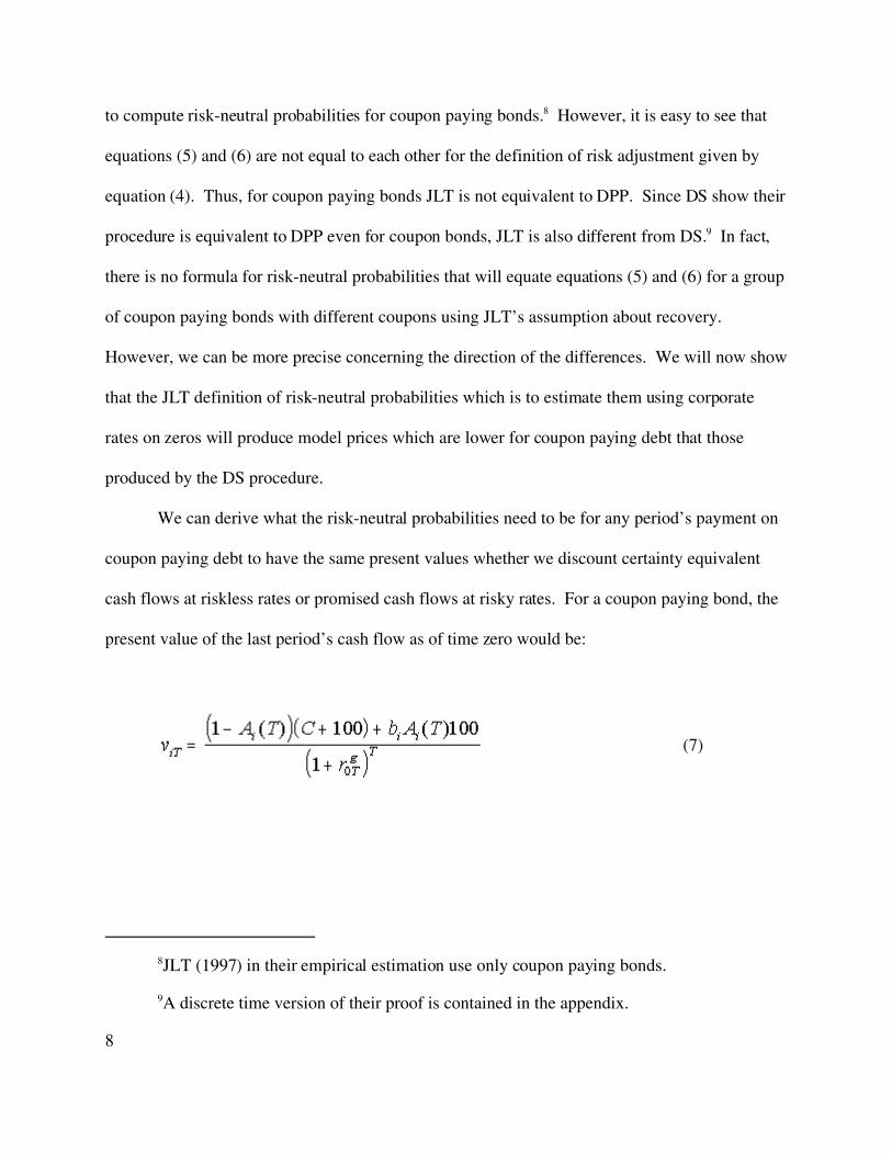
We can derive what the risk-neutral probabilities need to be for any period’s payment on

coupon paying debt to have the same present values whether we discount certainty equivalent

cash flows at riskless rates or promised cash flows at risky rates. For a coupon paying bond, the

present value of the last period’s cash flow as of time zero would be:

(7)

9

The first term represents the expected value of the coupon and principal in the last period of the

bond’s life while the second term represents the expected value of the cash flow if the bond goes

bankrupt at any time during its life. The lower case v indicates it is the present value of a single

cash flow rather than the complete bond value. Discounting the last period’s promised cash flow

at the corporate spot rate yields:

Equating these two equations and solving for yields

(8)

This expression for would result in the same bond value for the last periods cash flow

whether risk-neutral probabilities or DPP was used. Equation (4) would not do so.

10Note that since JLT assumes that cash from recovery at bankruptcy occurs at maturity,the cash recovered in bankruptcy only enters the last period of a bond’s life and not into cashflows in earlier periods.

10

If we examine the cash flows for any period prior to the period in which a bond matures,

the present value of the tth period cash flow using risk-neutral probabilities and continuing the

JLT assumption that all recovery from default occurs at the horizon is:10

and for promised cash flows the present value of the tth period cash flow is:

Equating and solving for yields:

(9)

11As an alternative to using the JLT procedure for estimating risk-neutral probabilities onecould directly estimate the probabilities that minimized the pricing error. The average pricewould no longer be biased but the same dispersion of errors as a function of coupon and maturitywould be present. The same problem is present when a structural model of the risk-neutralprobabilities is assumed and then the parameters of the model are estimated by finding those thatminimize pricing error. If the default assumption is the JLT default assumption, errors willdepend on the coupon and maturity.

11

By inspection, equation (4) results in a higher value for any than equation (8) or

(9). Thus using zero coupon bonds to define , the JLT procedure, leads to estimates of

that are larger than those obtained by determining using coupon paying bonds.

From equation (6) using higher ‘s results in lower prices. Thus using the JLT procedure

will always results in lower estimated prices than discounting promised cash flows at corporate

spot rates. Furthermore, from equation (8) the difference is a function of the coupon and the

more cash flows subject to this difference (the longer the maturity) the bigger the effect. Later

we will estimate and examine the size of this difference for coupon paying corporate bonds.11

Since JLT methodology leads to different values for coupon-paying corporate debt than

DS which is equivalent to discounting promised cash flows at corporate spot rates, the question

remains as to which provides more accurate valuation. Discounting promised cash flows at

corporate spot rates is correct only under restrictive assumptions, unlike governments where the

defense of using spots is an arbitrage argument. The arbitrage argument in terms of promised

payments is an approximation which is only exactly correct under certain assumptions. On the

other hand, the structure of the JLT model insures that coupon paying bond prices can’t be

reproduced exactly even over a fit period. The choice between these models then becomes an

empirical matter, one to which we now turn.

12The Warga database was discontinued shortly after our sample period.

13The only difference in the way CRSP data is constructed and our data is constructed isthat over the period of our study CRSP used an average of bid/ask quotes from five primarydealers called randomly by the New York Fed rather than a single dealer. However, comparisonof a period when CRSP data came from a single dealer and also from the five dealers surveyed13 by the Fed showed no difference in accuracy (Sarig and Warga, (1989)). See also thediscussion of pricing errors in Elton, Gruber, Agrawal and Mann (1999). Thus, our data shouldbe comparable in accuracy to the CRSP data.

12

II Testing the models

A. Data

Our bond data is extracted from the Lehman Brothers Fixed Income database distributed

by Warga (1998). This database contains monthly price, accrued interest, and return data on all

investment grade corporate and government bonds. In addition, the database contains descriptive

data on bonds including coupon, ratings, and callability. Our sample included ten years of

monthly data for the period from 1987 to 1996.12

A subset of the data in the Warga database is used in this study. First, any bond that is

matrix-priced rather than trader-priced in a particular month is eliminated from the sample for

that month. Employing matrix prices might mean that all our analysis uncovers is the formula

used to matrix price bonds rather than the economic influences at work in the market.

Eliminating matrix priced bonds leaves us with a set of prices based on dealer quotes. This is the

same type of data contained in the standard academic source of government bond data: the CRSP

government bond file.13

Next, we eliminate all bonds with special features that would result in their being priced

differently. This means we eliminate all bonds with options (e.g., callable or sinking fund), all

corporate floating rate debt, bonds with an odd frequency of coupon payments, government

14Slightly less than 3% of the sample was eliminated because of problematic data. Theeliminated bonds had either a price that was clearly out of line with surrounding prices (pricingerror) or involved a company or bond undergoing a major change.

15See Nelson and Siegal (1987). For comparisons with other procedures, see Green andOdegaard (1997) and Dahlquist and Svensson (1996). We also investigated the McCulloch cubic

13

flower bonds and index-linked bonds. Next, we eliminate all bonds not included in the Lehman

Brothers bond indexes because researchers in charge of the database at Shearson-Lehman

indicated that the care in preparing the data was much less for bonds not included in their

indexes. Finally, we eliminate bonds where the data is problematic.14 This resulted in

eliminating 2,710 bond months out of our sample of 95,278 bond months. Thus, the average

number of bonds in each month is about 770 bonds. A detailed breakdown of the number of

bonds in our sample categorized by maturity and risk is contained in Table 3. For classifying

bonds we use Moody’s ratings. In the few cases where Moody’s ratings do not exist, we classify

using the equivalent S&P rating.

B. Testing the Approaches

In this section we discuss the comparison of model errors produced by the DS procedure

(which is equivalent to discounting promised cash flows at corporate spot rates) with those

produced by discounting risk-adjusted cash flows at the riskless government rates using the JLT

definition of risk-neutral probabilities.

Calculation model prices using the discounting of promised cash flows is relatively

straightforward. First, spot rates must be calculated. In order to estimate spot rates from coupon

paying bonds, we used the Nelson Siegal (1987) procedure. For each rating category, including

governments, spots can be estimated as follows:15

spline procedures and found substantially similar results throughout our analysis. The Nelsonand Siegal model was fit using standard Gauss-Newton non-linear least squared methods. TheNelson and Siegal (1987) and McCulloch (1971) procedures have the advantage of using allbonds outstanding within any rating class in the estimation procedure, therefore lessening theeffect of sparse data over some maturities and lessening the effect of pricing errors on one ormore bonds. The cost of these procedures is that they place constraints on the shape of the yieldcurve. We used Moodys categories where they existed to classify bonds. Otherwise we used theequivalent S&P categories.

14

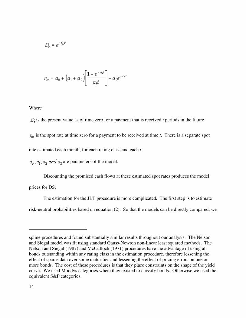
Where

is the present value as of time zero for a payment that is received t periods in the future

is the spot rate at time zero for a payment to be received at time t. There is a separate spot

rate estimated each month, for each rating class and each t.

are parameters of the model.

Discounting the promised cash flows at these estimated spot rates produces the model

prices for DS.

The estimation for the JLT procedure is more complicated. The first step is to estimate

risk-neutral probabilities based on equation (2). So that the models can be directly compared, we

16For a discussion of historical rates see Elton, Gruber, Agrawal and Mann (1999). Weuse continuous compounding in estimating risk neutral possibilities.

15

use the same estimates of spots that were used when we valued bonds using the DS procedure.

We used historical recovery rates for Aa, A, and Baa rated corporate bonds.16

In Table I we report the cumulative risk-adjusted probabilities we arrive at using this

procedure. Risk adjusted probabilities are usually defined in terms of the conditional risk

adjusted probability of going to default at time t given that default has not occurred earlier.

These conditional risk adjusted probabilities can be derived from Table 1 by taking

. While risk-adjusted probabilities are derived each month, in the interest of

brevity we report them once a year (January) for each year in our sample period and only for

industrial Baa bonds. It is interesting that the cumulative risk-neutral probabilities we arrive at in

Table 1 and for the unreported months are quite well-behaved relative to the cumulative risk-

neutral probabilities reported by other authors (e.g., Jarrow, Lando, Turnbull (1997). In

particular, our cumulative risk-neutral probabilities are not only positive, they increase with

maturity. From Table 1, risk-neutral probabilities (the change in the cumulative risk neutral

probabilities) are all positive. We attribute the greater plausibility of our results to the large

sample we use as well as the procedure we employ to extract spot rates.

As shown earlier, if one uses the JLT model, the risk-adjusted probabilities from zero

coupon bonds should understate the price of any coupon-paying bond. In addition, we should

expect that the absolute errors (a measure of dispersion) should be higher since the errors

themselves should be a function of the coupon and coupons vary within any rating class.

16

Table II shows that the empirical results are consistent with what theory suggests for JLT

and DS procedures applied to coupon paying bonds. Note, as shown in Table II Panel A, that

when bonds are priced by the DS model, the average error for each class of bonds is very close to

zero and overall the average error is less than one cent per $100 bond. The fact that average

errors are small and unbiased is not surprising for it indicates that the Nelson and Siegal

approach to extracting spots is unbiased and that the DS assumption about discounting promised

payments by risky spots leads to unbiased results. The same is not true for the JLT procedure.

When we look at the average pricing errors from the JLT procedure, we see that they are negative

and quite large for any class of bonds. Errors are measured as model price minus invoice price.

The negative error shows that the JLT procedure applied to coupon-paying bonds produces

model prices that underestimate their market value. In addition, as shown in Table II Panel B the

average absolute error is much higher for the JLT procedure. Average absolute errors are an

indication of how well a procedure fits the large number of bonds in each risk class. To the

extent that a model value is affected by characteristics of a bond such as coupon and maturity,

average absolute errors should be greater and a function of the characteristic. The average

absolute error is affected by both the mean error and the dispersion across bonds. Table 2C

corrects for the mean error by computing the average absolute error around the mean. Since the

average error for DS is close to zero, this correction has little effect on DS and the average

absolute errors in 2B and 2C are similar. Since there is a large mean error for JLT, calculating

average absolute errors around the mean does make a difference for JLT. However, even after

this correction, absolute JLT errors are much higher than absolute DS errors. Thus, the JLT

procedure not only has a mean bias, but also results in greater dispersion of errors around the

17To judge the realism of these numbers once can compare average absolute errors ofcorporate bonds to analogous errors in other studies. The numbers seem reasonable. Forexample, Elton, Gruber, Agrawal and Mann (2001) come up with an estimate of .210 forgovernment bonds. The DS absolute error for AA bonds are about 50% higher.

17

mean across bonds. These results are exactly what our analytical examination of the models lead

us to expect.17

It is worth examining one more point. We would not expect the average error to be a

function of maturity when we discount promised payments. With the JLT procedure we would

expect the error to increase as maturity increases. This pattern occurs because each coupon is

systematically undervalued and the more coupons a bond pays, the larger the mispricing. This is

exactly what happens, as shown in Table III. For example, for the JLT procedure applied to

BBB industrial bonds, the error increases from thirteen cents per $100 to over $3 per $100 as

maturity increases. While it is possible to correct the JLT results so that ex post it has a mean

error equal to zero, the dispersion of the error within a risk class and the relationship of error with

coupon and maturity will still hold.

VI Conclusion

In this paper we explore the ability of two rating-based models to price corporate bonds.

These models involve discounting promised cash flows at the estimated spot rates (DS) and risk-

neutral valuation using the definition of risk-neutral probabilities proposed by JLT. These

models were selected because they are the most widely used and because most other rating based

models use one of these as their foundation. We show that the JLT risk-neutral probabilities are

independent of estimates of the transition matrix and default probability. We then show that

18

when we examine coupon paying bonds that the JLT risk-neutral probabilities result in lower

model prices than the DS procedure. Furthermore, the JLT procedure causes pricing errors to be

functions of both maturity and coupon size. The reason for this is that there is no formula for

risk-neutral probabilities that can simultaneously equate risk-neutral valuation to valuation using

promised flows for both zeros and coupon debt. Discounting promised cash flows at the

corporate spot rates (the DS procedure) is unbiased, and has lower errors and a smaller dispersion

than the JLT model.

TABLES Table I

Risk Neutral Probabilities of Default This table shows Ai(t), the cumulative risk neutral probabilities of default after t years, conditional on initial rating being i. These numbers are computed from the spot rates of treasury (r0t

g) and corporate bonds (r0tc) using the expression,

Ai(t) = (1/(1-bi))[1-exp(-t(r0t

c-r0tg))]

where bi is the recovery rate for rating i. The numbers shown are for Baa rated bonds of Industrial category with maturity t = 1 to t = 11 years.

t=1 t=2 t=3 t=4 t=5 t=6 t=7 t=8 t=9 t=10 t=11 Jan-87 0.0230 0.0519 0.0802 0.1070 0.1328 0.1578 0.1823 0.2064 0.2302 0.2536 0.2766 Jan-88 0.0433 0.0775 0.1031 0.1236 0.1416 0.1582 0.1742 0.1898 0.2052 0.2205 0.2356 Jan-89 0.0178 0.0340 0.0544 0.0779 0.1028 0.1284 0.1540 0.1794 0.2045 0.2293 0.2538 Jan-90 0.0233 0.0450 0.0711 0.1002 0.1309 0.1619 0.1928 0.2234 0.2535 0.2832 0.3123 Jan-91 0.0196 0.0711 0.1185 0.1587 0.1941 0.2267 0.2578 0.2878 0.3171 0.3458 0.3740 Jan-92 0.0277 0.0719 0.1060 0.1308 0.1500 0.1665 0.1815 0.1959 0.2099 0.2237 0.2374 Jan-93 0.0191 0.0662 0.1035 0.1300 0.1501 0.1667 0.1818 0.1960 0.2099 0.2235 0.2370 Jan-94 0.0143 0.0381 0.0607 0.0812 0.1003 0.1185 0.1362 0.1536 0.1708 0.1878 0.2046 Jan-95 0.0133 0.0300 0.0485 0.0678 0.0874 0.1069 0.1264 0.1456 0.1647 0.1836 0.2023 Jan-96 0.0113 0.0248 0.0416 0.0603 0.0798 0.0997 0.1196 0.1393 0.1589 0.1784 0.1976

Table II DPP Errors and JLT Errors

This table compares the average pricing errors when promised payments are discounted at the corporate rates called DPP prices and JLT fitted prices for coupon bonds. Discounted rates on promised payments were fitted each month separately for each rating category of bonds and DPP errors are the DPP fitted prices minus the invoice prices of coupon bonds. JLT model parameters were estimated using the zero coupon prices obtained from the DPP estimation. These parameter estimates were then used to compute the JLT fitted prices of the coupon bonds. JLT errors are the JLT fitted prices minus the invoice prices of coupon bonds. Errors are expressed in dollars on bonds with face value of 100 dollars. Panel (A): Average pricing errors with signs preserved

Estimation Method Financial Sector Industrial Sector Aa A Baa Aa A Baa

DPP -0.0094 -0.0104 -0.0149 -0.0162 -0.0082 0.0094 JLT -0.6256 -1.0954 -1.3308 -0.7414 -1.2216 -1.3485

Panel (B): Average absolute pricing errors

Estimation Method Financial Sector Industrial Sector Aa A Baa Aa A Baa

DPP 0.2983 0.5042 0.8584 0.4537 0.5905 1.1348 JLT 0.6913 1.2177 1.5766 0.8985 1.3366 1.7489

Panel (C): Average absolute pricing error around mean

Estimation Method Financial Sector Industrial Sector Aa A Baa Aa A Baa

DPP 0.2977 0.5028 0.8566 0.4505 0.5897 1.1367 JLT 0.5793 0.9734 1.2706 0.6976 1.0208 1.3941

Table III

DPP and JLT Errors sorted by Maturity Panel (B) and (C) of this table show the average errors from discounting the promised payments and from using the JLT procedure respectively, sorted by maturity. The errors are model prices minus the invoice prices. Panel (A) shows the number of coupon bonds over which the averages were taken. All errors are in dollars on bonds with face value of one hundred dollars.

Panel (A): Number of bonds over which the averages were taken

Maturity Range Financial Sector Industrial Sector Aa A Baa Aa A Baa

[1,2) years 1862 5036 1357 638 2069 1110 [2,4) years 2948 9309 2357 1214 4065 2841 [4,6) years 1993 7141 2169 1091 4602 2995 [6,8) years 1201 6002 2270 980 4153 2930

[8,10) years 897 6072 2700 1135 4502 3759 [10,11) years 62 667 224 167 731 346

Panel (B): Average errors from discounting the promised payments

Maturity Range Financial Sector Industrial Sector Aa A Baa Aa A Baa

[1,2) years -0.0414 -0.0501 -0.1000 -0.0744 -0.0428 -0.0190 [2,4) years 0.0393 0.0341 0.0685 0.0159 0.0134 0.0192 [4,6) years -0.0707 -0.0870 -0.1022 -0.0661 -0.0541 -0.0558 [6,8) years -0.0560 -0.0137 -0.0516 -0.0135 -0.0009 0.0660

[8,10) years 0.1047 0.0584 0.0611 0.0451 0.0364 0.0298 [10,11) years -0.1367 -0.1094 -0.0777 -0.1334 -0.0568 -0.1153

Panel(C): Average JLT errors

Maturity Range Financial Sector Industrial Sector Aa A Baa Aa A Baa

[1,2) years -0.1188 -0.1520 -0.2245 -0.1403 -0.1236 -0.1268 [2,4) years -0.2506 -0.3377 -0.3035 -0.1865 -0.3180 -0.3760 [4,6) years -0.7849 -0.9660 -1.0123 -0.5806 -0.8852 -1.0144 [6,8) years -1.2003 -1.5959 -1.7349 -0.9487 -1.4886 -1.5303 [8,10) years -1.6716 -2.4409 -2.5563 -1.4735 -2.3305 -2.3878

[10,11) years -2.2844 -3.4263 -3.0599 -1.9294 -3.1267 -3.3157

19

APPENDIX

Equivalency of DPP and DS for Coupon Bonds

In this section we make the following recovery assumption: at the time of bankruptcy the

investor receives a constant fraction of the market value of a similarly rated non-bankrupt bond

of the same maturity, and the same fraction of the coupon payment. We will prove that with this

definition of recovery, a risk-neutral probability (of default) exists that produces the same value

for any bond whether one used corporate spot rates to discount promised payments or

government spot rates to discount expected cash flows which are derived from certainty

equivalent risk-neutral probabilities.

We will use the notation employed earlier with the following additions:

1. Superscripts P and R indicate the bond is valued by discounting promised cash

flows (P) or risk-neutral valuation (R).

2. is the forward rate as of the time the bond is being valued from t to t+1.

3. We have dropped the i subscript associated with rating class. All variables should

be interpreted as belonging to rating class i.

Define the risk-neutral probability of bankruptcy by:

(A-1)

20

We show below that for the definition of bankruptcy we are examining and the definition

of risk-neutral probabilities given by equation (A-1), the value of any coupon or zero coupon

bond will be exactly the same whether we use corporate rates to discount promised cash

payments or government spot rates to discount risk-neutral cash flows.

Consider a T period bond. If the bond is solvent at the horizon, its promised payment is

the same as its risk-adjusted payment. Therefore, .

Then, for period T-1, the value of the bond based on risk-neutral valuation is:

Or

21

Substituting in equation (A-1) yields

If we value the bond by discounting promised payments at the risky spot rate

Since the right-hand side of the above equations are identical:

By iterating the valuation process backward, we can write out the expression for

and and with identical substitution prove they were equal. This will hold for any

period for any bond. Furthermore, setting C equal to zero does not change the identities so the

definition of risk-neutral probabilities given by equation (A-1) holds for zero coupon bonds as

well as coupon-paying bonds.

Thus, with the recovery rate defined as a fraction of the value of the firm plus the coupon,

the value of the bond is identical whether one discounts promised payments at the corporate spot

rate or discounts risk-neutral payments at the government rate. The results are independent of

maturity or coupon on the bonds.

22

Bibliography

Black, F. and M. Scholes (1973). The Pricing of Options and Corporate Liabilities. Journal of

Political Economy, 81: 637-654.

Claessen and Pennacchi (1996). Estimating the Likelihood of Mexican Default From the Price of

Brady Bonds. Journal of Financial and Quantitative Analysis, 31.

Collins-Dufresne, P. and B. Solnik (2001). On the Term Structure of Default Premia on the

Swap and Libor Markets. Forthcoming, Journal of Financem LVI (3), 1095-1115

Cumby, B. and M. Evans (1995). The Term Structure of Credit Risk: Estimates and

Specification Tests. Department of Economics, Georgetown University.

Das, S. and P. Tufano (1996). Pricing Credit Sensitive Debt when Interest Rates and Credit

Spreads are Stochastic. Journal of Financial Engineering, 5: 161-198.

Das, S. (1999). Pricing Credit Derivatives. In J. Francis, J.Frost, and J. G. Whittaker (editors),

Handbook of Credit Derivatives, 101-138.

Duffee, G. (1998). The Relation Between Treasury Yields and Corporate Bond Yield Spreads.

Journal of Finance, 53:6, 2225-2240.

23

Duffie, D and D. Lando (2001). Term Structures of Credit Spreads with Incomplete Accounting

Information. Econometrics 69, 633-664.

Duffie, D. and K. Singleton (1997). Modeling Term Structures of Defaultable Bonds. Review of

Financial Studies 12: 687-720.

Elton, E., M. Gruber, D. Agrawal and C. Mann (2001). Explaining the Rate Spread on Corporate

Bonds. Journal of Finance, 56, 1: 247-277.

Jarrow, R., D. Lando and S. Turnbull (1997). A Markov Model for the Term Structure of Credit

Spreads. Review of Financial Studies, 10: 481-523.

Jones, E., S. Mason and E. Rosenfeld (1984). Contingent Claims of Analysis of Corporate

Capital Structures: An Empirical Investigation. Journal of Finance, 39: 611-625.

Lando, D. (1997). Modeling Bonds and Derivatives with Default Risk. In M. Dempster and S.

Pliska (editors), Mathematics of Derivative Securities, pp. 369-393, Cambridge University Press.

Lando, D. (2000). Some Elements of Rating-Based Credit Risk Modeling. In N. Jegadeesh and

B. Tuckman (editors), Advanced Tools for the Fixed Income Professional. John Wiley & Son,

193-215.

24

Longstaff, F. and E. Schwartz (1995). A Simple Approach to Valuing Risky Fixed and Floating

Rate Debt. Journal of Finance, 50, 3: 789-819.

Madan, D. B. and H. Unal (1998). Pricing the Risks of Default. Review of Derivatives

Research, 2, 121-160.

Madan, D. B. and H. Unal (2000). A Two-Factor Hazard Rate Model for Pricing Risky Debt and

the Term Structure of Credit Spreads. Journal of Financial and Quantitative Analysis.

Merrick, J. (1999). Crisis Dynamics of Implied Default Recover Rates: Evidence from Russia

and Argentina. Working paper, New York University.

Merton, R. (1974). On the Pricing of Corporate Debt: The Risk Structure of Interest Rates.

Journal of Finance, 29: 449-470.

Sarig, O. and A. Warga (1989). Bond Price Data and Bond Market Liquidity. Journal of

Financial and Quantitative Analysis, 24: 367-378.