1

IS THERE A RISK PREMIUM IN

CORPORATE BONDS?

by Edwin J. Elton,* Martin J. Gruber,*

Deepak Agrawal** and Christopher Mann**

* Nomura Professors of Finance, Stern School of Business, New York University

** Doctoral students, Stern School of Business, New York University

1 Most of the models using option pricing techniques assume a zero risk premium. Bodie, Kane, and Marcus (1993) assume the spread is all default premium. See alsoFons (1994) and Cumby and Evans (1995). On the other hand, Jarrow Lando andTurnbull (1997) and Das-Tufano (1996) assume that any risk premium impounded incorporate spreads is captured by adjusting transition probabilities.

2

INTRODUCTION

In recent years there have been a number of papers examining the pricing of corporate debt.These papers have varied from theoretical analysis of the pricing of risky debt using option pricingtheory, to a simple reporting of the default experience of various categories of risky debt. The vastmajority of the articles dealing with corporate spreads have examined yield differentials of interest-paying corporate bonds relative to government bonds.

The purpose of this article is to reexamine and explain the differences in the rates offered oncorporate bonds and those offered on government bonds (spreads), and in particular to examinewhether there is a risk premium in corporate bond spreads. As part of our analysis, we show thatdifferences in corporate and government rates should be measured in terms of spot rates rather thanyield to maturity.

Differences in spot rates between corporates and government bonds (the corporate spotspreads) differ across rating classes and should be positive for four reasons:

1. Default premium -- some corporate bonds will default and investors require a higher promisedpayment to compensate for the expected loss on default.

2. Tax premium – interest payments on corporate bonds are taxed at the state level while interestpayments on government bonds are not.

3. Liquidity effect ) corporate bonds have higher and more changeable bid ask spreads and theremay be a delay in finding a counter party for a transaction. Investors need to be compensatedfor these risks.

4. Risk premium – corporate bonds are riskier than government bonds, and investors may requirea premium for the higher risk.

The only controversial part of the above analysis is the fourth point. Some authors in theiranalysis assume that the risk premium is zero in the corporate bond market.1

The analysis in this paper has major implications for a series of articles which have appeared in

2 See for example Altman (1989), Goodman (1989), Blume, Keim and Patel (1991), and Cornell and Green (1991).

3 There is another aspect of liquidity that is not explicitly measured in this paper but islikely to show up in the risk premium. This type of risk involves the fact that debtmarkets may be illiquid at the very times when liquidity is most needed. We believe thatthis risk to the extent that it exists will be captured in sensitivity of spreads to the macrorisk factors employed in the final section of this paper.

3

the literature of Financial Economics. Several of these articles indicate that low-rated bonds producehigher average returns than bonds with higher ratings.2 In addition, Blume, Keim and Patel (1991) showthat the standard deviation of returns is no higher for low-rated bonds than it is for high-rated bonds.This evidence has been used to argue that low-rated bonds are attractive investments. Ourdecomposition of corporate spreads into a default premium, tax premium and risk premium sheds newlight on these results. As we will show, the tax and risk premium are substantial, and are higher for lowrated bonds than for high rated bonds, and thus the conclusion that low-rated bonds are superiorinvestments may be incorrect for almost all investors.

The major purpose of this paper is to see if a risk premium exists or if the first three reasons canaccount for the size of actual spreads that are observed. In the rest of the paper, we will not dealdirectly with liquidity. Most corporate bonds are held over a long time period. Thus, the differences inbid ask spread between governments and corporates averaged over this long horizon is very small.3 This paper proceeds as follows: In the first section, we present a description of the data employed inthis study. A large sample of corporate bonds which include only option-free dealer-priced bonds isconstructed. In the second section we present the methodology for, and present the results of,extracting government and corporate spot rates from data on individual bonds. We then examine thedifferentials between the spot rates which exist for corporate bonds and those that exist for governmentbonds. We find that the corporate spot spreads are higher for lower rated bonds, and that they tend togo up with increased maturity. The shape of the spot spread curve can be used to differentiate betweenalternative corporate bond valuation models derived from option pricing theory.

Before turning to a decomposition of the corporate spot spreads into their component parts, theability of estimated spot rates to price corporate bonds is examined. How bad is the approximation?We answer this by examining pricing errors on corporates using the spot rates extracted from oursample of corporate bonds.

The remainder of this paper is concerned with decomposing corporate spreads intoparts that are due to the default premium, tax premium, and risk premium. In the third section of thispaper we model and estimate that part of the corporate spread which is due to the default premium. Ifwe assume, for the moment, that there is no risk premium, then we can value corporate bonds under a

4 We also temporarily ignore the tax disadvantage of corporate bonds relative to government bonds in this section.

4

risk neutrality assumption.4 This risk neutral assumption allows us to construct a model of the corporatespot spread and estimate it using historical data on rating transition probabilities default rates, andrecovery rates after default. The spot rate spread curves estimated by incorporating only defaultpremiums is well below the observed spot spread curve and doesn’t increase as we move to lowerratings as fast as the observed spot curves do. The difference between these curves can only be dueto taxes and possibly risk aversion.

In the next section of this paper we examine the impact of both the default premium and taxpremium on corporate spot spreads. In particular, we build taxes into the risk neutral valuation modeldeveloped earlier and estimate the set of spot rates that should be used to discount promised cashpayments when taxes and default premiums are taken into consideration. We show that using the bestestimate of tax rates and historical rating transition probabilities, and recovery rates, actual corporatespot spreads are still much higher than taxes and default premiums can account for. Furthermore, fixingtaxes at a rate that explains the spread on AA debt still doesn’t explain the difference in A and BBBspreads. The difference in spreads across rating categories has to be due to the presence of riskaversion. Furthermore, to explain empirical spreads the compensation the investor requires for risk mustgo up as risk increases and as maturity increases.

The last section of this paper presents direct evidence of the existence of a risk premium by firstrelating the time series of spreads to a set of variables that are generally considered systematic factorsimpacting risk in the literature of Financial Economics and then by relating cross sectional differences inspreads to sensitivities of each spread to those variables. We have already shown that the defaultpremium and tax premium can only partially account for the difference in corporate spreads. In thissection we present direct evidence that there is a risk premium by showing that part of the corporatespread, not explained by defaults or taxes, is related to systematic factors that are generally believed tobe priced in the market.

I. DATA

Our bond data is extracted from the Lehman Brothers Field Income database distributed byWarga (1998). This database contains monthly price, accrued interest, and return data on all investmentgrade corporate and government bonds. In addition, the database contains descriptive data on bondsincluding coupon, ratings, and callability.

A subset of the data in the Warga database is used in this study. First, all bonds that werematrix-priced rather than trader-priced were eliminated from the sample. Employing matrix prices might

5 The only difference in the way CRSP data is constructed and our data is constructed is that over the period of our study CRSP used an average of bid/ask quotes from five primary dealers called randomly by the New York Fed rather than a single dealer. However, comparison of a period when CRSP data came from a single dealer and also from the five dealers surveyed by the Fed showed no difference in accuracy (Sarig and Warga (1989)). See also the discussion of

pricing errors in Section 2. Thus our data should be comparable in accuracy to theCRSP data.

6 The methodology used to do this is described later in this paper. We also examined $3and $4 filters. Employing a $3 or $4 filter would have eliminated few other bonds, sincethere were few intermediate-size errors, and we could not find any reason for the errorwhen we examined the few additional bonds that would be eliminated.

5

mean that all our analysis uncovers is the formula used to matrix price bonds rather than the economicinfluences at work in the market. Eliminating matrix priced bonds leaves us with a set of prices based ondealer quotes. This is the same type of data contained in the standard academic source of governmentbond data: the CRSP government bond file.5

Next, we eliminated all bonds with special features that would result in their being priceddifferently. This meant we eliminated all bonds with options (e.g. callable or sinking fund), all corporatefloating rate debt, bonds with an odd frequency of coupon payments, government flower bonds andindex-linked bonds.

Next, we eliminated all bonds not included in the Lehman Brothers bond indexes becauseresearchers in charge of the database at Shearson-Lehman indicated that the care in preparing the datawas much less for bonds not included in their indexes. This resulted in eliminating data for all bonds witha maturity of less than one year.

Finally, we eliminated bonds where the data was problematic. This involved examining the dataon bonds which had unusually high pricing errors. Bond pricing errors were examined by filtering onerrors of different sizes and a final filter rule of $5 was selected.6 Errors of $5 or larger are unusual, andthis step resulted in eliminating 2,710 bond months out of our total sample of 95,278 bond months.Examination of the bonds eliminated because of large pricing errors showed that the errors were due tothe following three reasons:

1. The price was radically different from both the price immediately before the large error and theprice after the large error. This probably indicates a mistake in recording the data.

2. The company issuing the bonds was going through a reorganization that changed the nature of

6

the issue (such as its interest rate or seniority of claims), and this was not immediately reflectedin the data shown on the tape, and thus the trader was likely to have based the price oninaccurate information about the bond’s characteristics.

3. A change was occurring in the company that resulted in the rating of the company changing sothat the bond was being priced as if it were in a different rating class.

We need to examine one further issue before leaving this section. The prices in the LehmanBrothers are bid prices as are the institutional price data reported in DRI or Bloomberg. Since thedifference in the bid and ask price in the government market is less than this difference in the corporatemarket, using bid data would result in a spread between corporate and government bonds even if theprice absent the bid ask spread were the same. How big is this bias? Discussion with ShearsonLehman, indicates that for the bonds in our sample (active corporate issues) the average spread wasabout 25 cents per $100. Elton and Green (1998) show the average spread for governments is 5 cents.Thus, the bias is (25 -5)/2 or about 10 cents. We will not adjust the spreads shown in our tables but thereader should realize they are about 10 cents too high.

II. TERM STRUCTURE OF SPOTS?

In this section of the paper, we examine the difference in spot rates between corporate bondsand Treasury bonds over various maturities. Our analysis has three parts. In the first part, we explainwhy we examine spot rates rather than yield to maturity. In the second part, we present themethodology for extracting spot rates and present the term structure of spreads over our sample period.In the third part, we examine the pricing errors which result from valuing corporate and governmentbonds using estimated spot rates.

A. Why Spots?

Most previous work on corporate spreads has defined corporate spread as the differencebetween the yield to maturity on a corporate bond (or an index of corporate bonds) and the yield tomaturity on a government bond (or an index of government bonds) of the same maturity. This traditiongoes back at least as far as Fisher (1959). Although most researchers now recognize that there areproblems with using yield to maturity, given the long tradition, a few comments might be helpful.

The basic reason for using spots rather than yield to maturity is that arbitrage arguments holdwith spot rates, not yield to maturity. Thus, finding two riskless coupon bonds with different yields tomaturity and the same maturity date does not indicate an arbitrage opportunity, whereas finding tworiskless zeros with different spot rates and the same maturity indicates a profitable arbitrage. In additionmany authors use yield to maturity on an index of bonds. Published indexes use a weighted average ofthe yields of the component bonds to compute a yield to maturity on the index. Yields are not additive,

7 Even spot rates on promised payments are not a perfect mechanism for pricing riskybonds because the law of one price will hold as an approximation when applied topromised payments rather than risk adjusted expected payments.

8 See Nelson and Siegal (1987). For comparisons with other procedures, see Green and Odegaard (1997) and Dahlquist and Svensson (1996). We also investigated the McCulloch cubic spline procedure and found substantially similar results

throughout our analysis. The Nelson and Siegal model was fit using standard Gauss-Newton non-linear least squared methods.

7

so this is not an accurate way of calculating the yield to maturity on an index.

When we consider corporate bonds, another problem arises that does not hold with risklessbonds; the spread in the yield to maturity on corporates relative to governments can change even ifthere is no change in any of the fundamental factors that should affect spread, namely taxes, defaultrates and risk premiums. In particular, the difference in the yield to maturity on corporates and the yieldto maturity on governments is a function of the term structure of governments. Inferences made aboutchanges in risk in the corporate market because of the changing spread in yield-to-maturity may beerroneous since the changes can be due simply to changes in the shape of the government termstructure. Thus, in this paper we examine spreads in spot rates.7

B. The Term Structure of Corporate Spreads

In this section, we examine the corporate government spread for bonds in different risk classesand with different maturities. While there are several methods of determining spot rates from a set ofbond prices, both because of its simplicity and proven success in deriving spots, we have adopted themethodology put forth by Nelson and Siegel (N&S).8 The N&S methodology involves fitting thefollowing equations to all bonds in a given risk category to obtain the spot rates that are appropriate forany point in time.

D etr tt= −

r a a ae

a ta et o

a ta t= + +

−

−−

−( )1 23

2

1 33

WhereDt = the present value as of time zero for a payment that is received t periods in the futurert = the spot rate at time zero for a payment to be received at time ta0, a1, a2, and a3 = parameters of the model.

The N&S procedure is used to estimate spot rates for different maturities for both Treasury

9 The Nelson and Siegal (1987) and McCulloch (1971) procedures have the advantageof using all bonds outstanding within any rating class in the estimation procedure,therefore, lessening the affect of sparse data over some maturities and lessening theaffect of pricing errors on one or more bond. The cost of these procedures is that theyplace constraints on the shape of the yield curve.

10 For some of our analysis, we used Moodys data and for part S&P data. To avoid confusion we will always use S&P classifications though we will identify the sources ofdata. When we refer to BBB bonds as rated by Moodys, we are referring to theequivalent Moodys class, namely Baa.

11 This difference is not surprising for industrial and financial bonds differ both in theirsensitivity to systematic influences and idiosyncratic shocks which occurred over thetime period.

8

bonds and for bonds within each corporate rating class for every month over the time period January1987 through December 1996. This estimation procedure allows us on any date, to use corporatecoupon and principle payments and prices of all bonds within the same rating class to estimate the fullspot yield (discount rate) curve which best explains the prices of all bonds in that rating class on thatdate.9

As mentioned earlier, the data we use on risky bonds only exists for bonds of maturity longerthan one year. In addition, for most of the ten-year period studied the number of AAA bonds thatexisted and were dealer quoted was too small to allow for accurate estimation of a term structure.Finally, data on corporate bonds rated below BBB was not available for most of the time period westudied.10 Because of this, spot rates are only computed for bonds with maturities between two to tenyears for Treasury, AA, A and BBB-rated bonds. Initial examination of the data showed that the termstructure for financials was slightly different from the term structure for industrials, and so in this sectionthe results for each sector are reported separately.11

We are concerned with measuring differences between corporates and governments. Thecorporate spread we examine is the difference between the spot rate on corporate bonds in a particularrating class and spot rates for Treasury bonds of the same maturity. Table I presents Treasury spotrates as well as corporate spreads for our sample of the three rating classes discussed earlier: AA, Aand BBB for maturities from two to ten years. In Panel A of Table I, we have presented the averagedifference over our ten-year sample period, 1987-1996. In Panels B and C we present results for thefirst and second half of our sample period. We expect these differences to vary over time. In a latersection, we will examine the time pattern of these differences, as well as variables which might accountfor the time pattern of the differences. For the moment, let us examine the shape of the averagerelationship.

12 While the BBB industrial curve is consistent with the models that are mentioned,estimated default rates shown in Table IV are inconsistent with the assumptions thesemodels make. Thus the humped BBB industrial curve is inconsistent with spread beingdriven only by defaults.

9

There are a number of interesting results reported in these tables. Note that in general thecorporate spread for a rating category is higher for financials than it is for industrials. For both financialand industrial bonds, the corporate spread is higher for lower-rated bonds for all spots across allmaturities in both the ten-year sample and the five-year subsamples. Bonds are priced as if the ratingscapture real information. To see the persistence of this influence, Figure 1 presents the time pattern ofthe spreads on six-year spot payments for AA, A and BBB industrial bonds month by month over theten-years of our sample. Note that the curves never cross. A second aspect of interest is therelationship of corporate spread to the maturity of the spot rates. An examination of Table I shows thatthere is a general tendency for the spreads to increase as the maturity of the spot lengthens. However,for the ten years 1987-1996 and each five year sub-period the spread on BBB industrial bonds exhibitsa humped shape.

The results we find can help differentiate between the corporate debt valuation models derivedfrom option pricing theory. The upward sloping spread curve for high-rated debt is consistent with themodels of Merton (1974), Jarrow, Lando and Turnbull (1997), Longstaff and Schwartz (1995), andPitts and Selby (1983). It is inconsistent with the humped shape derived by Kim, Ramaswamy andSundaresan (1987). The humped shape for BBB industrial debt is predicted by Jarrow, Lando andTurnbull (1997) and Kim, Ranaswamy and Sundaresan (1987), and is consistent with Longstaff andSchwartz (1995) and Merton (1974) if BBB is considered low-rated debt.12

We will now examine the results of employing spot rates to estimate bond prices.

C. Fit Error

One test of how well the spot rates extracted from corporate yield curves explain prices in thecorporate market is to directly compare actual prices with the theoretical prices derived by discountingcoupon and principal payments at the estimated spot rates. Theoretical price and actual price candiffer because of errors in the actual price and because bonds within the same rating class, as definedby a rating agency, are not homogenous in risk. We calculated theoretical prices for each bond in eachrating category every month using the estimated spot yield curves estimated for that rating class in thatmonth. Each month the square root of the average squared error (actual minus theoretical price) iscalculated. This is then averaged over the full ten years and separately for the first and last five years foreach rating category. The average root mean squared error between actual price and estimated price isshown in Table II. The average error of 21 cents per 100 dollars for Treasuries is comparable to the

10

average root mean squared error found in other studies. Elton and Green (1998) showed averageerrors of about 16 cents per $100 using GovPX data over the period June 1991 to September 1995.GovPX data are trade prices, yet the difference in error between the studies is quite small. Green andOdegaard (1997) used the Cox Ingersoll and Ross (1987) procedure to estimate spot rates using datafrom CRSP. While their procedure and time period are different from ours, their errors again are aboutthe same as those we find for government bonds in our data set (our errors are smaller). The data setand procedures we are using seem to produce comparable size errors in pricing government bonds tothose found by other authors.

The average pricing errors become larger as we examine lower grade of bonds. Averagepricing errors are over twice as large for AA’s as for Treasuries. The pricing errors for BBB’s arealmost twice those of AA’s, with the errors in A’s falling in between. Thus default risk leads not only tohigher spot rates, but also to greater uncertainty as to the appropriate value of the bond, and this isreflected in higher pricing errors. This is an added source of risk and may well be reflected in higher riskpremiums, a subject we investigate shortly. There is little change in pricing errors over the two five-yearperiods.

III DEFAULT SPREADS

To estimate a risk premium and later see what influences affect it, it is necessary to examinehow much of the corporate spread is explained by both the default premium and state taxes. Initially wewill examine the effect of the default premium by itself. Thus, initially, we will examine the magnitude ofthe spread under risk neutrality with the tax differences between corporates and governments ignored.Later we will introduce tax differences and examine whether default spreads and taxes together aresufficient to explain the observed spot spread.

Under risk neutrality, the expected cash flows would be discounted at the government bondrate to obtain the corporate bonds’ value. Recall that corporate spreads are estimated using promisedspot curves. Consider a two-period bond using expected cash flows and risk neutrality. For simplicity,assume its par value at maturity is $1. We wish to determine its value at time zero and we do sorecursively by valuing it first at time 1 (as seen at time 0) and then at time 0. Its value as of time one when it is a one-period bond has three component parts: the value of theexpected coupon to be received at 2, the value of the expected principal to be received at 2 if the bondgoes bankrupt at 2, and the value of the principal if the bond survives where all expectations areconditional on the bond surviving to period 1. This can be expressed as

(1)V C P aP P e rG

12 2 2 21 1 12= − + + − −[ ( ) ( )]

Where is the coupon rateC

is the probability of bankruptcy in period t conditional on no bankruptcy in an earlier periodPt

13 We discount at the forward rate. For this is the rate which can be contracted at timezero for moving money across time.

11

is the recovery rate assumed constant in each perioda

is the forward rate as of time 0 from t to t+1 for government (risk-free) bonds13rttG+1

is the value of a T period bond at time t given that it has not gone bankrupt in an earlier period.VtT

Alternatively valuing the bond using promised cash flows, its value is:

(2)V C e rC

12 1 12= + −( )

Where

1. Is the forward rate from t to t+1 for corporate bondsrt tC

+1

Equating the two values and rearranging to solve for the difference between corporate and governmentforward rates, we have:

(3)e PaP

Cr rC G− − = − + +

( ) ( )( )

12 12 112

2

at time zero, the value of the two-period bond using risk neutral valuation is

(4)V C P aP P V e r G

02 1 1 1 121 1 01= − + + − −[ ( ) ( ) )]

and using promised cash flows, its value is

V C V e rC

02 1201= + −[ ]

Equating these equations and solving for the difference in one period spot (or forward) rates, we have

(5)e PaP

V C

rC

rG− −

= − ++

( )(1 )01 01

11

12

In general, in period t the difference in forward rates is

(6)e PaP

V Cr r

tt

t T

ttC

ttG− −

++

+

+ + = − + +( ) ( )1 1 1 1

1

1

Where1. VTT = 1

14 This problem is discussed in an earlier footnote. The issue is that arbitrage should holdfor risk adjusted cash flows; thus discount rates on promised cash flows are anapproximation.

15 We examined alternative reasonable estimates for coupon rates and found only secondorder effects in our results. While this might seem inconsistent with equation (6), notethat from the recursive application of equation (1) and (2) changes in C are largelyoffset by opposite changes in V.

16 Each row of the transition matrix shows the probability of having a given rating in oneyear contingent on starting with the rating specified by the row.

17 Technically it is the last column of the squared transition matrix.

12

Obviously this difference in forward rates varies across bonds with different coupons, even forbonds of the same rating class. Thus the estimates of spot rates obtained empirically are averagesacross bonds with different coupons, and one single spot rate does not hold for all bonds. Nevertheless,given the size of the pricing error found in the previous section, assuming one rate is a goodapproximation.14

We can now use equation (6) to obtain estimates of the default spreads on corporate bonds.The inputs to equation (6) were obtained as follows: First, the coupon was set so that a ten-year bondwith that coupon would be selling close to par in all periods.15 Then, estimates of default rates andrecovery rates were computed. To estimate future default rates we used a transition matrix and adefault vector. We employed two separate estimates of the transition matrix, one estimated by S&P(See Altman (1997)) and one estimated by Moody’s (Carty & Fons(1994)).16 These are the twoprincipal rating agencies for corporate debt. The transition matrixes are shown in Table III.

The probability of default given a particular rating at the beginning of the year is shown as thelast column in Table III. Given the transition matrix and an initial rating, we can estimate the probabilityof a default in each future year, given that the bond has not defaulted prior to that year. In year one, theprobability of default can be determined directly from the transition matrix and default vector, and iswhatever proportion of that rating class defaults in year one. To obtain year two defaults, we first usethe transition matrix to calculate the ratings going into year two for any bond starting with a particularrating in year 1. Year two defaults are then the proportion in each rating class times the probability thata bond in that class defaults by year-end.17 Table IV shows the default probabilities by age, and initialrating class for the Moodys and S&P transition data. The entries in this table represent the probabilityof default for any year t given an initial rating and given that the bond was not in default at time t-1.

Table IV shows the importance of rating drift over time on default probabilities. The marginal

18 These default probabilities as a function of age are high relative to prior studies e.g.,Altman (1997), Moody’s (1998).

13

probability of default increases for the high rated debt and decreases for the low rated debt. Thisoccurs because bonds change rating class over time.18 For example, a bond rated AAA by S&P haszero probability of defaulting one year later. However, given that it hasn’t previously defaulted, itsprobability of defaulting twenty years latter is .206%. In the intervening years some of the bondsoriginally rated AAA have migrated to lower-rated categories where there is some probability ofdefault. At the other extreme, a bond originally rated CCC has a probability of defaulting equal to22.052% in the next year, but if it survives twenty more years the probability of default is only 2.928%.If it survives twenty years the bond is likely to have a higher rating. Despite this drift, 20 years laterbonds which were rated very highly at the beginning of the period tend to have a higher probability ofstaying out of default after twenty years than do bonds which had a low rating. However ratingmigration means this does not hold for all risk classes. For example, note that after 12 years theconditional probability of default for CCC’s is lower than the default probability for B’s. Why? Examining Table III shows that the odds of being upgraded to investment grade conditional on notdefaulting is higher for CCC than B. Eventually, bonds that start out as CCC and continue to exist willbe higher rated than those that start out as B’s. In short, the small percentage of CCC bonds thatcontinue to exist for many years, end up at higher ratings on average than the larger percentage of Bbonds that continue to exist for many years.

In addition to estimates of the probability of default, we need estimates of recovery rates fordefaulted bonds. The estimates available for recovery rates by rating class are computed as a functionof the rating at time of issuance. Table V shows these recovery rates. Thus of necessity we assume thesame recovery rate independent of the maturity of the bond and that the recovery rate of a bondcurrently ranked AA is the same as a newly issued AA bond.

Employing equation (6) along with the default rates from Table IV, the recovery rates fromTable V, and the coupon rates estimated as explained earlier allows us to calculate the risk neutral zerotax default spread in forward rates. This is then converted to an estimate of the default spread in spotrates.

Table VI shows the zero tax default spread under risk neutral valuation. The first characteristicto note is the size of the tax-free default spread relative to the empirical corporate spread discussedearlier. The zero tax default spread is very small and does not account for much of the corporatespread. This can be seen graphically in Figure 2 for A rated industrial bonds. One factor that couldcause us to underestimate the default spread is that our transition matrix estimates are not calculatedover exactly the same period for which we estimate the spreads. However, there are three factors thatmake us believe that we have not underestimated default spreads. First, our default estimates shown in

14

Table IV are higher than those estimated in other studies. Second, the average default probabilities overthe period where the transition matrix is estimated by Moody’s and S&P are close to the averagedefault probabilities in the period we estimate spreads (albeit default probabilities in the latter period aresomewhat higher). Third, the S&P transition matrix which was estimated in a period with higher averagedefault probability and more closely matches the years in which we estimate spread results in lowerestimates of defaults. However, as a further check on the effect of default rates, we calculated thestandard deviation of year-to-year default rates over the 20 years ending 1996. We then increased themean default rate by two standard deviations. This resulted in a maximum increase in spread for AA’sof .004% and .023% for BBB’s. Thus, even with extreme default rates, default premiums are too smallto account for the observed spreads. It also suggest that changes in default premiums over time are toosmall to account for any significant of the change in spreads over time.

Also note from Table VI the zero tax risk neutral default spread of AA’s relative to BBB’s.While the spread for BBB’s is higher, the difference in spreads because of differences in defaultexperience is much less than the differences in the empirical corporate spreads. Differences in defaultrates cannot explain the differences in spreads between bonds of various rating classes. This stronglysuggests that differences in spreads must be explained by other influences, such as taxes or riskpremiums. The second characteristic of default spreads to note is the pattern of spreads as the maturityof the spot rate increases. The spread increases for longer maturity spots. This is the same pattern weobserve for the empirical spreads shown in Table I. However, for AA and A the increase in defaultpremiums with maturity is less than the increase in the empirical corporate spread.

IV. TAX SPREADS

Another difference between government bonds and corporate bonds is that the interestpayments on corporate bonds are subject to state tax with almost all maximum marginal rates between five and ten percent. Since state tax is deductible at the federal level, the burden of state tax is reducedby the federal rate. Nevertheless, state taxes could be a major contributor to the spreads. For example,if the coupon was 10% and effective state taxes were 5%, state taxes alone would result in a 1/2%spread (.05 x .10). To analyze the impact of state taxes on spreads, we introduced taxes into theanalysis developed in the prior section. For a one-period bond maturing at $1, the basic valuationequation after state taxes is:

(7)V C P t t aP a P t t P es g s grG

01 1 1 1 11 1 1 1 1 1 01= − − − + + − − + − −[ ( )( ( )) ( ) ( ( )) ( )]

where

1. is the government forward rate (which is the spot rate in Period 1).rG01

2. ts is the state tax rate3. tg is the federal tax rate4. other terms as before

19 We tried alternative coupons. The spread is reasonably insensitive to changes in thecoupon and none of the discussion would change with reasonable variations in thecoupon.

20 See Commerce Clearing House (1997)

15

Equation (7) has two terms that differ from the prior section. The change in the first term represents thepayment of taxes on the coupon. The new third term is the tax refund due to a capital loss if the bonddefaults.

The valuation equation on promised cash flows is

V C e rC

01 1 01= + −[ ]

Solving for the difference between corporate and government rates, we have

(8)e PaP

C

C P a P

Ct tr rs g

C G− − = − + + −− − −

+ −( ) ( )[ ( ) ( ) ]

( )( )01 01 11

1 11

111 1 1

The first two terms are identical to the terms shown before where only default risk is taken intoaccount. The last term is the new term that captures the effect of taxes. Taxes enter it in two ways.First, the coupon is taxable and its value is reduced by taxes and is paid with probability (1-P1).Second, if the firm defaults (with probability P1), the amount lost in default is a capital loss and taxes arerecovered. Note that since state taxes are a deduction against federal taxes, the marginal impact of statetaxes is ts(1-tg).

As in the prior section, these equations can be generalized to the T period case. The finalequation is

(9)( )[ ( ) ( ) )]

( ) ( )11 1

111

1

1 1

1

1 1− ++

−− − −

+− =+

+

+

+ +

+

− −+ +PaP

C V

C P a P

C Vt t et

t

t T

t t

t Ts g

r rttC

ttG

This equation is used to estimate the forward rate spread because of default risk and taxes.

The inputs were determined as follows: The coupon was set so that a ten-year bond would sellat par.19 The same probabilities of default and recovery rates were used as were used when wecalculated the default premium in the last section. Table IV gives the default probabilities as a functionof time, and Table V the recovery rates. State taxes and federal taxes are more difficult to estimate. Weused three procedures. First we looked at state tax codes. For most states, maximum marginal statetax rates range between 5% and 10%.20 Since the marginal tax rate used to price bonds should be aweighted average of the active traders, we assumed that a maximum marginal tax rate would beapproximately the mid-point of the range of maximum state taxes, or 7.5%. In almost all states, state taxfor financial institutions (the main holder of bonds) is paid on income subject to federal tax. Thus, ifinterest is subject to maximum state rates, it must also be subject to maximum federal tax, and we

21 For smaller institutions it is 34%.

22 One other estimate in the literature that we are aware of is that produced by Severenand Stewart (1992 ) who estimate state taxes at 5%.

16

assume the maximum federal tax rate of 35%.21

Our second attempt at estimating taxes was to directly determine the effective tax rate (state taxrate adjusted for a federal rate) that best explained market prices. We examined eleven different valuesof effective tax rates ranging from 0% to 10% in steps of one percent. For each tax rate we estimatedthe after tax cash flow for every bond in every month in our sample. This was done using cash flows asdefined in the multi-period version of equation (7). Then for each month, rating class and tax rate weestimated the spot rates using the Nelson Siegal procedure discussed in section II-B, but now appliedto after tax expected cash flows. These spot yield curves are then applied to the appropriate after taxexpected cash flows to price all bonds in each rating class in each month. The difference between thiscomputed price and the actual price is calculated for each tax rate. The tax rate which resulted in thesmallest mean square error between calculated price and actual price is determined. When we do sowe find that an effective tax rate of 4% results in the smallest mean square pricing error. In addition, the4% rate produced errors that were significantly lower (at the five percent significance level) than anyother rate except 3%. Since the errors were lower on average with the 4% rate we employed this ratefor later analysis.22 For the first two estimates of effective taxes we obtain corporate spreads shown inpanel A and B of Table VII. In doing so we convert the forward rates determined from equation (9) tospot rates. Note first that the spreads are less than those found empirically as shown in Table I and thatfor our best estimate of effective state taxes (4%), state taxes are more important than default inexplaining spreads. Recall that increasing default probabilities by two standard deviations only increasedthe spread for AA bonds by .003%. Thus increasing defaults to an extreme historical level plusmaximum or estimated tax rates are insufficient to explain the corporate spreads found empirically.

However, there is a fair amount of uncertainty as to the appropriate tax rates. Thus weemployed one final procedure to try to see if tax rates and default risk are together sufficient to explainspreads. Since AA bonds have the lowest default probabilities in our sample, we would expect the riskpremium on these bonds to be smaller than the risk premium on lower rated bonds. If we assume thatthe risk premium on these bonds is zero, we can get an estimate of the tax rate that is necessary toexplain AA spreads. The effective state tax rate needed to explain AA spreads is 6.7%. There aremany combinations of federal and state taxes that are consistent with this number. However, as notedabove, since state tax is paid on federal income, it is illogical to assume a high state rate without acorresponding high federal rate. Thus the only pair of rates that would explain spreads on AA’s is astate tax rate of 10.3% and a federal rate of 35%. There are very few states with a 10% rate. Thus, it ishard to explain spreads on AA bonds with taxes and default rates.

23 Even if the institutional bankruptcy risk is small, the consequences of an individual issuebankruptcy on a managers career may be so significant as to induce decision makers torequire a substantial premium.

17

Furthermore, we see no reason why the tax factor should differ for AA or BBB bonds. We canapply the tax factor of 6.7% that explains AA spread to A and BBB rated bonds. When we do so, weget the estimated spreads shown in Table VII, Panel C. Note that the rates determined by using the riskneutral valuation model on expected values, and the tax rates that explain the spreads on AA debtunderestimate the spreads on A and BBB bonds. Taxes, default rates, and whatever risk premium thatis inherent in AA bonds underestimate the corporate spread on lower rated bonds. Furthermore, asshown in Table VII, Panel C, the amount of the underestimate goes up as the quality of the bondsexamined goes down. The inability of tax and default rates to explain the corporate spread for AAseven at extreme tax rates, and the inability to explain the difference in spreads between AA’s andBBB’s suggest a non zero risk premium.

Figure II shows the default and tax premium for A industrials where the tax premium is basedon our best estimate of effective state taxes (4%). Note, once again, that state taxes are moreimportant than the default premium in explaining spreads. State taxes are ignored in most modeling ofthe spread (see Jarrow, Lando and Turnbull (1997), Das and Tufano (1996) and Duffee (1998)). Thissuggests that this modeling direction is unlikely to be very useful in explaining real bond prices.

V. RISK PREMIUMS

As shown in the last section, default premiums and state tax rates are insufficient to explain thespread in corporate bonds. This suggests the existence of a risk premium. There are two issues thatneed to be addressed. First what causes a risk premium and second, given the small size of the defaultpremium why is the risk premium so large.

There are several reasons why one might expect a risk premium, even with a small averagedefault premium. First, we might expect a risk premium because bankruptcies tend to cluster in timeand institutions are highly levered, so that even with low average bankruptcy loses there is still asignificant chance of financial difficulty at an uncertain time in the future and we need a premium tocompensate for this risk.23 Second, if corporate bond prices move systematically with other assets inthe market while government bonds do not, then we might require a risk premium to compensate forthe non-diversifiability of corporate bond risk, just like we would for any other asset. There are tworeasons why bond risk might be systematic. First if default risk were to move with market prices, so asstock prices rise default risk goes down and as they fall it goes up, it would introduce a systematic

24 Two other explanations of the relationship between term premium and corporatespread might be the relationship between government term premiums and default risk.Given the small impact of changes in default probability on spread this cannot be asignificant explanation of the relationships.

18

factor. Second, the risk premium required in the capital market might change over time. If the changingrisk premium effects both corporate bond and stock markets, then this would introduce a systematicinfluence. We shall now demonstrate that such a relationship exists and explains most of the riskpremium. We shall do so in two parts: first, relating unexplained spreads (corporate spreads less bothdefault premium and tax premium as determined from equation (9)) to systematic risk factorsformulated from government spot data, and then relating unexplained spread to variables which havebeen used as systematic risk factors in the pricing of common stocks. By studying how the unexplainedspread is related to risk factors we can estimate its size and see if it is explained by the systematicfactors. Throughout we will assume a 4% effective state tax rate which is our estimate from the priorsection.

A. Term Structure Risk Premiums

In this section we explore the relationship between the time series behavior of the unexplainedpart of the corporate government spread and attributes of the government spot yield curve. We use twoattributes of the government bond spot curve, the level and the long/short spread. These characteristicswere selected because they have been shown to be the systematic risk factors explaining governmentbond returns (see Elton, Gruber and Michaely (1990) Litterman and Sheinkman (1991)). The level ofrates is related to con-current inflation expectations, while “term spread” on governments is related tolong-term versus short-term expectations about inflation, uncertainty about future rates of inflation, andthe market reaction to the pricing of this uncertainty.24

When current inflation expectations increase we would expect government rates to increase andbecause we are in a riskier environment, we would expect the corporate spread to increase. Inaddition, the corporate government spread should increase when the level of government ratesincreases because of the impact of state taxes. A rise in the level of government rates causes a highertax burden on corporate bond holders and to maintain after tax relationships the spread must increase.

When the term spread on governments goes up we would also expect to see an increase in theunexplained spread on corporate bonds, if it contains a risk premium. A rise in the government termspread could be caused by greater uncertainty about future interest rates or an increase in thecompensation for risk demanded by investors. An increase in the uncertainty of future interest rates inlikely to mean greater default risk and a higher corporate government spread. Likewise, an increase in

25 An increase in the term spread will also cause the spread or long bonds to increasemore than the spread on short maturity bonds because of the impact of state taxes.

26 The number of AA industrial bonds that have a maturity between one and ten years forour sample is fairly small, and thus spot rates for this rating class are estimated with lessprecision. There are many more AA financials, and when we examine this group thecoefficients on both variables are positive and significant. However, the financial samplesuffers from not having many BBB rated bonds.

19

compensation for risk should apply equally to the corporate premium as it does to the term premiumand lead to an increase in the corporate government spread.25

We are trying to examine whether the unexplained spread between corporates andgovernments is explained by interest rate factors. To estimate the monthly unexplained spread betweencorporates and governments we subtracted from each months estimated spread the part of the spreadexplained by default and taxes as determined by equation (9). This produced a time series ofunexplained spreads, one for each risk class (AA, A, BBB) for each maturity. These time series ofrisk premiums were regressed on the two bond factors in the following regression.P a B Y B T et m c t t t, , = + + +1 2

Where(1) equals the estimated unexplained spreads in month t for maturity m and rating class C.Pt mc, ,

(2) is the two-year government spot rate at time t.Yt

(3) is the term spread on government bonds measured by the ten-year spot rate minus the twoTt

year spot rate(4) are constantsa B B, ,1 2

The results of this regression for industrial bonds are presented in Table VIII. Note that theresults are consistent with our expectations. First note that the unexplained spread is positively relatedto both the government interest rate level variable and the term spread at the 5% level of statisticalsignificance except for some of the shorter maturity spots in the AA class.26 This is a very strongindication that the unexplained portion of corporate spreads contain a risk premium and which is relatedto bond factors. The existence of a risk spread is also strongly supported by the fact that for anymaturity spot, the regression coefficient on the government yield spreads gets larger as we move tolower quality bonds (from AA to A to BBB). These results are consistent with the existence of a riskpremium in the pricing of corporate bonds.

This type of regression has been estimated by Longstaff and Schwartz (1995) and Duffee

27 Duffee recognizes that the signs should be positive, and explores what in his analysismight result in a negative sign.

20

(1998). Both find negative signs where ours are positive.27 The positive sign is appropriate. As justdiscussed when interest rates rise the state tax rises and the spread must increase to compensate for thetax. In addition, rising interest rates have preceded almost all recessions. Since defaults increase inrecessions, rising interest rates should be associated with higher expected defaults and a bigger spread.

B. Spreads and Standard Risk Measures

In this section we explore the extent to which the sensitivity to factors, which have been shownto explain common stock expected returns can explain the unexplained spread. That portion of theunexplained spread which is accounted for by sensitivity to systematic risk factors can be identified as arisk premium. In order to examine the impact of sensitivities on unexplained spreads we need tospecify a return generating model. We can write a general return generating model as

(10)R a f et j jt tj

= + +∑ β

for each year (two through ten) and each rating classWhere1. is the return during month t. Rt

2. is the sensitivity of changes in the spread to factor j.β j

3. is return on factor j during month t. The factors are each formulated as the difference inf jt

return between two portfolios (zero net investment portfolios).

While this process holds for returns we want to relate it to the metric that we are investigatingthe unexplained spread. If and are the spot rates on a corporate and government bond ofrt m

c, rt m

G,

maturity m at time t respectively then the price of a pure discount bond with face value 1 is

P et mc r mt m

c

,,= − ⋅

P et mG r mt m

G

,,= − ⋅

and one month latter the price of an m period corporate or government bond is

P et mc r mt m

c

+− ⋅= +

11,

,

P et mG r mt m

G

+− ⋅= +

11,

,

28 This is not the total return on holding a corporate or government bond, but rather theportion of the return due to changing spread (the term we wish to examine).

29 We used two multi-factor models, the Connor Korajczyk empirically derived modeland the multi-factor model tested by us earlier see Elton, Gruber and Blake (1998). These results will be discussed in footnotes. We thank Bob Korajczyk for supplying uswith the monthly returns on the Connor Korajczyk factors.

30 The results are almost identical using the Connor Korajczyk empirically derived factorsor the Elton, Gruber and Blake (1998) model. When a single factor model is used, 20out of 27 betas are significant with an R2 of about .10.

21

That part of the return on an m period bond from t to t+1 due to a change in spread is28

( )Re

em r rt t

cr m

r m t mc

t mc

t mc

t mc, , ,ln,

+

− ⋅

− ⋅ += = −+

1 1

1,

and

( )Re

em r rt t

Gr m

r m t mG

t mG

t mG

t mG, , ,ln,

+

− ⋅

− ⋅ += = −+

1 1

1,

and

(11)( ) ( )[ ]R R m r r r r m Pt tc

t tG

t mc

t mG

t mc

t mG

t m c, , , , , , , ,+ + + +− = − − − − = −1 1 1 1 ∆

Thus the difference in return between corporate and government due to a change in spread is equal tominus m times the change in spread.

There are many forms of a multi-index model which we could employ to study unexplainedspreads. We chose to concentrate our results on the Fama French model because of its wide use in theliterature but we investigated other models including the single index model and some of the results willbe discussed in footnotes.29 The Fama French model employs the excess return on the market, thereturn on a portfolio of small stocks minus the return on a portfolio of large stocks and the return on aportfolio of high minus low book to market stocks as its three factors.

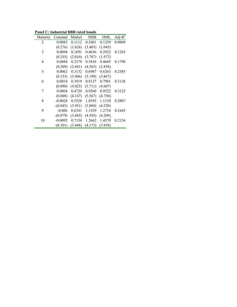
Table IX shows the results of regressing return of corporates over governments derived fromthe change in unexplained spread for industrial bonds (as in equation (11)) against the Fama Frenchfactors. The regression coefficient on the market factor is always positive and is statistically significant20 out of 27 times. This is the sign we would expect on the basis of theory. This holds for the FamaFrench market factor, and also holds (see Table IX) for the other Fama French factors representingsize and book to market ratios. The return is positively related to small minus big and high minus lowbook to market.30 Notice that the sensitivity to all of these factors tends to increase as maturity

31 Employing a single index model using sensitivity to the excess return on the S&P index,

leads to of .21 and .43 for industrial and financial bonds respectively..R2

22

increases and to increase as quality decreases. This is exactly what would be expected if we wereindeed measuring risk factors. Examining financials shows similar results except that the statisticalsignificance of the regression coefficients and the size of the is higher for AA’s. R2

It appears that the change in spread not related to taxes or expected defaults is at least in part

explained by factors which have been successful in explaining returns over time in the equity market.We will now turn to examining cross sectional differences in average unexplained premiums. If there isa risk premium for sensitivity to stock market factors then the expected value of this net or unexplainedpremium should be linearly related to the sensitivities of the unexplained premiums (the ’s fromβ

equation (10)) and differences in sensitivities should explain differences in the unexplained premiumacross corporate bonds of different maturity and different rating class. We have 27 unexplainedspreads for industrial bonds and 27 for financial bonds since maturities range from class 2, through 10,and there are three rating classifications. When we regress unexplained spread against sensitivities forindustrial bonds the cross sectional adjusted for degrees of freedom is .32, while for financials it isR2

.58. We have been able to account for almost 1/3 of the difference in unexplained premiums forcorporates and more than1/2 for financial bonds.31

Another way to examine this is to ask how much of the unexplained spread can the sensitivitiesaccount for. That is for each maturity and risk class of bonds what is the size of the unexplained spreadthat existed versus the size of the risk premium that is accounted for by the sensitivity of the bonds tothe three factors times the price of these factors over the time period. For industrials the average riskpremium is .813, while just employing the sensitivities we would estimate it to be .660. For financial,the actual risk premium is .934 but using the estimated beta and prices it is .605. In short, 85% of theindustrial unexplained spread is accounted by the three risk sensitivities while for financials it is 67%. Note that whether we use the cross sectional explanatory power or the size of the estimate relative tothe realized risk premium one sees that standard risk measures have been able to account for a highpercentage of the unexplained spread.

One more set of tests was tried. There are two reasons that could explain why unexplainedspreads are related to sensitivity to the Fama French factors. The first is that the Fama French factorsare proxying for changes in default expectations. We are measuring the impact of changing defaults. Thus, in cross section, the sensitivity of unexplained spreads to the factors may in part be picking up themarket price of systematic changes in default expectations. The second explanation is that riskpremiums change simultaneously across all markets, and thus spreads are systematic. In either case wehave a risk premium. Nevertheless, it is useful to see if changes in default expectations account for amajor part of the risk premium. To test this we added several measures of changes in default risk to

23

equation (10) as a fourth factor. We tried actual changes (perfect forecasting) and several distributedlag and lead models. None of the results were statistically significant or had consistent signs acrossdifferent groups of bonds.

In this section we have shown that the unexplained spread is related to the term structure ofgovernment bond spot rates. The long-short spread has often been used as a risk variable, and the levelis related to state tax obligations. We have also shown that the change in unexplained spread is relatedto factors that are considered systematic in the stock market. Modern risk theory states that systematicrisk needs to be compensated for and thus, common equity has to earn a risk premium. Changes incorporate spreads lead to changes in return on corporates and thus, returns on corporates are alsosystematically related to common stock factors with the same sign as common equity. If common equityreceives a risk premium for this systematic risk then corporate bonds must also earn a risk premium.We have shown that sensitivity to the factors that are used to explain risk premiums in common stocksexplain between 1/3 and ½ of the spread in corporate and government rates that is not explained by thedifference between promised and expected payments and taxes. This is strong evidence of theexistence of a risk premium of a magnitude that has economic significance.

24

CONCLUSION

In this paper, we have examined the size and cause of differences in spot rates on corporatebonds relative to government bonds. We have discussed the methodology for arriving at, and the resultsfrom looking at, corporate spot spreads. The properties of the corporate spot spread are useful inexamining the reasonableness of alternative corporate bond valuation models derived from optionpricing. We then examine the three components of the corporate spot spread: a default premium, a taxpremium, and unexplained portion. We show that the default premium is quite small compared to theoverall corporate spread. Differential taxes, on the other hand, can potentially be a major factor inaccounting for the overall corporate spread. Finally, of key significance, our results indicate that a largepart of the remainder of the spread appears to be a risk premium in the pricing of corporate debt. Weshow that the corporate spread has a strong relationship to priced systematic risk factors which havebeen found to account for both bond and stock returns in the literature of Financial Economics. Furthermore, differences in the size of the unexplained spread is related to differences in the sensitivityto the systematic factors.

There has been a lot of modeling in the corporate bond area. One of the purposes of this paperis to provide empirical facts that a model needs to reflect in order to be consistent with actual spreads. In particular, we show that state taxes explain part of the spread and that the risk premium is partially acompensation for systematic components in the financial markets and not just compensation forincreased default risk. These empirical facts cause serious difficulties for models that explain corporatebond prices by changing default rates and transition probabilities, so that the price curve is fit (seeJarrow, Lando and Turnbull(1994)) and related models. Since state taxes and sensitivities to riskfactors are likely to change over time, those using this approach will need to build models where “riskadjusted” transition matrixes change over time. To capture state tax effects these models would needtransition matrixes to change as a function of the level of rates. To capture the systematic risk factorsthe transition matrix and default rates would need to change as a function of changes in the systematicfactors. This is likely to place too great a demand on the models and hence other modeling strategiesthat explicitly account for taxes and systematic factors are likely to be more productive than continuingto develop ways of fitting spreads by changing transition matrixes. In addition, in deciding on whetherone should purchase any class of bond, the investor needs to know the size of the compensation theyare receiving for bearing risk. Models that lump everything into a changing transition matrixes do notprovided this needed information.

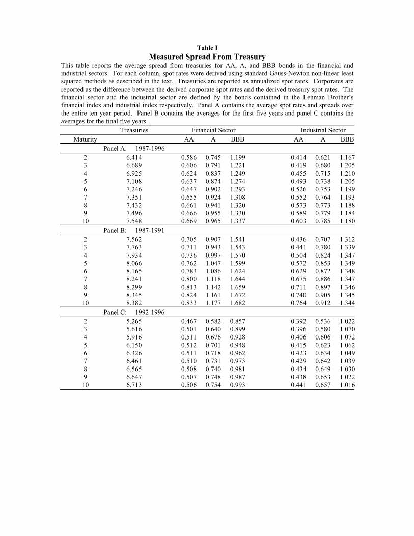
Table IMeasured Spread From Treasury

This table reports the average spread from treasuries for AA, A, and BBB bonds in the financial andindustrial sectors. For each column, spot rates were derived using standard Gauss-Newton non-linear leastsquared methods as described in the text. Treasuries are reported as annualized spot rates. Corporates arereported as the difference between the derived corporate spot rates and the derived treasury spot rates. Thefinancial sector and the industrial sector are defined by the bonds contained in the Lehman Brother’sfinancial index and industrial index respectively. Panel A contains the average spot rates and spreads overthe entire ten year period. Panel B contains the averages for the first five years and panel C contains theaverages for the final five years.

Treasuries Financial Sector Industrial SectorMaturity AA A BBB AA A BBB

Panel A: 1987-19962 6.414 0.586 0.745 1.199 0.414 0.621 1.1673 6.689 0.606 0.791 1.221 0.419 0.680 1.2054 6.925 0.624 0.837 1.249 0.455 0.715 1.2105 7.108 0.637 0.874 1.274 0.493 0.738 1.2056 7.246 0.647 0.902 1.293 0.526 0.753 1.1997 7.351 0.655 0.924 1.308 0.552 0.764 1.1938 7.432 0.661 0.941 1.320 0.573 0.773 1.1889 7.496 0.666 0.955 1.330 0.589 0.779 1.184

10 7.548 0.669 0.965 1.337 0.603 0.785 1.180Panel B: 1987-1991

2 7.562 0.705 0.907 1.541 0.436 0.707 1.3123 7.763 0.711 0.943 1.543 0.441 0.780 1.3394 7.934 0.736 0.997 1.570 0.504 0.824 1.3475 8.066 0.762 1.047 1.599 0.572 0.853 1.3496 8.165 0.783 1.086 1.624 0.629 0.872 1.3487 8.241 0.800 1.118 1.644 0.675 0.886 1.3478 8.299 0.813 1.142 1.659 0.711 0.897 1.3469 8.345 0.824 1.161 1.672 0.740 0.905 1.345

10 8.382 0.833 1.177 1.682 0.764 0.912 1.344Panel C: 1992-1996

2 5.265 0.467 0.582 0.857 0.392 0.536 1.0223 5.616 0.501 0.640 0.899 0.396 0.580 1.0704 5.916 0.511 0.676 0.928 0.406 0.606 1.0725 6.150 0.512 0.701 0.948 0.415 0.623 1.0626 6.326 0.511 0.718 0.962 0.423 0.634 1.0497 6.461 0.510 0.731 0.973 0.429 0.642 1.0398 6.565 0.508 0.740 0.981 0.434 0.649 1.0309 6.647 0.507 0.748 0.987 0.438 0.653 1.022

10 6.713 0.506 0.754 0.993 0.441 0.657 1.016

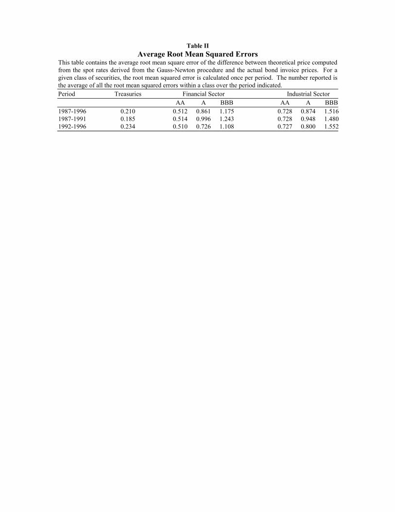
Table IIAverage Root Mean Squared Errors

This table contains the average root mean square error of the difference between theoretical price computedfrom the spot rates derived from the Gauss-Newton procedure and the actual bond invoice prices. For agiven class of securities, the root mean squared error is calculated once per period. The number reported isthe average of all the root mean squared errors within a class over the period indicated.Period Treasuries Financial Sector Industrial Sector

AA A BBB AA A BBB1987-1996 0.210 0.512 0.861 1.175 0.728 0.874 1.5161987-1991 0.185 0.514 0.996 1.243 0.728 0.948 1.4801992-1996 0.234 0.510 0.726 1.108 0.727 0.800 1.552

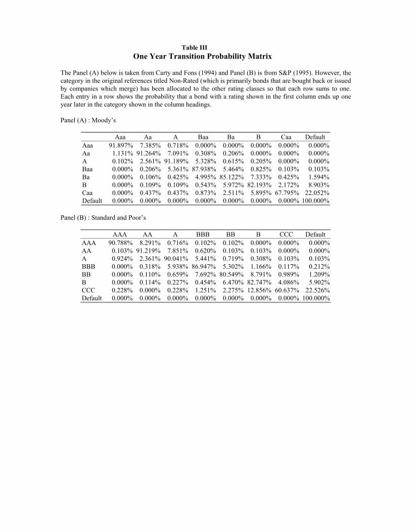
Table IIIOne Year Transition Probability Matrix

The Panel (A) below is taken from Carty and Fons (1994) and Panel (B) is from S&P (1995). However, thecategory in the original references titled Non-Rated (which is primarily bonds that are bought back or issuedby companies which merge) has been allocated to the other rating classes so that each row sums to one.Each entry in a row shows the probability that a bond with a rating shown in the first column ends up oneyear later in the category shown in the column headings.

Panel (A) : Moody’s

Aaa Aa A Baa Ba B Caa DefaultAaa 91.897% 7.385% 0.718% 0.000% 0.000% 0.000% 0.000% 0.000%Aa 1.131% 91.264% 7.091% 0.308% 0.206% 0.000% 0.000% 0.000%A 0.102% 2.561% 91.189% 5.328% 0.615% 0.205% 0.000% 0.000%Baa 0.000% 0.206% 5.361% 87.938% 5.464% 0.825% 0.103% 0.103%Ba 0.000% 0.106% 0.425% 4.995% 85.122% 7.333% 0.425% 1.594%B 0.000% 0.109% 0.109% 0.543% 5.972% 82.193% 2.172% 8.903%Caa 0.000% 0.437% 0.437% 0.873% 2.511% 5.895% 67.795% 22.052%Default 0.000% 0.000% 0.000% 0.000% 0.000% 0.000% 0.000% 100.000%

Panel (B) : Standard and Poor’s

AAA AA A BBB BB B CCC DefaultAAA 90.788% 8.291% 0.716% 0.102% 0.102% 0.000% 0.000% 0.000%AA 0.103% 91.219% 7.851% 0.620% 0.103% 0.103% 0.000% 0.000%A 0.924% 2.361% 90.041% 5.441% 0.719% 0.308% 0.103% 0.103%BBB 0.000% 0.318% 5.938% 86.947% 5.302% 1.166% 0.117% 0.212%BB 0.000% 0.110% 0.659% 7.692% 80.549% 8.791% 0.989% 1.209%B 0.000% 0.114% 0.227% 0.454% 6.470% 82.747% 4.086% 5.902%CCC 0.228% 0.000% 0.228% 1.251% 2.275% 12.856% 60.637% 22.526%Default 0.000% 0.000% 0.000% 0.000% 0.000% 0.000% 0.000% 100.000%

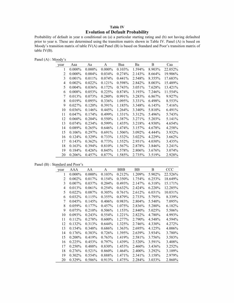
Table IVEvolution of Default Probability

Probability of default in year n conditional on (a) a particular starting rating and (b) not having defaultedprior to year n. These are determined using the transition matrix shown in Table IV. Panel (A) is based onMoody’s transition matrix of table IV(A) and Panel (B) is based on Standard and Poor’s transition matrix oftable IV(B).

Panel (A) : Moody’syear Aaa Aa A Baa Ba B Caa

1 0.000% 0.000% 0.000% 0.103% 1.594% 8.903% 22.052%2 0.000% 0.004% 0.034% 0.274% 2.143% 8.664% 19.906%3 0.001% 0.011% 0.074% 0.441% 2.548% 8.355% 17.683%4 0.002% 0.022% 0.121% 0.598% 2.842% 8.003% 15.489%5 0.004% 0.036% 0.172% 0.743% 3.051% 7.628% 13.421%6 0.008% 0.053% 0.225% 0.874% 3.193% 7.246% 11.554%7 0.013% 0.073% 0.280% 0.991% 3.283% 6.867% 9.927%8 0.019% 0.095% 0.336% 1.095% 3.331% 6.498% 8.553%9 0.027% 0.120% 0.391% 1.185% 3.348% 6.145% 7.416%

10 0.036% 0.146% 0.445% 1.264% 3.340% 5.810% 6.491%11 0.047% 0.174% 0.499% 1.331% 3.312% 5.496% 5.743%12 0.060% 0.204% 0.550% 1.387% 3.271% 5.203% 5.141%13 0.074% 0.234% 0.599% 1.435% 3.218% 4.930% 4.654%14 0.089% 0.265% 0.646% 1.474% 3.157% 4.678% 4.258%15 0.106% 0.297% 0.691% 1.506% 3.092% 4.444% 3.932%16 0.124% 0.329% 0.733% 1.532% 3.022% 4.229% 3.662%17 0.143% 0.362% 0.773% 1.552% 2.951% 4.030% 3.435%18 0.163% 0.394% 0.810% 1.567% 2.878% 3.846% 3.241%19 0.184% 0.426% 0.845% 1.578% 2.806% 3.676% 3.074%20 0.206% 0.457% 0.877% 1.585% 2.735% 3.519% 2.928%

Panel (B) : Standard and Poor’syear AAA AA A BBB BB B CCC

1 0.000% 0.000% 0.103% 0.212% 1.209% 5.902% 22.526%2 0.002% 0.017% 0.154% 0.350% 1.754% 6.253% 18.649%3 0.007% 0.037% 0.204% 0.493% 2.147% 6.318% 15.171%4 0.013% 0.061% 0.254% 0.632% 2.424% 6.220% 12.285%5 0.022% 0.087% 0.305% 0.761% 2.612% 6.031% 10.031%6 0.032% 0.115% 0.355% 0.879% 2.733% 5.795% 8.339%7 0.045% 0.145% 0.406% 0.983% 2.804% 5.540% 7.095%8 0.059% 0.177% 0.457% 1.075% 2.836% 5.280% 6.182%9 0.075% 0.210% 0.506% 1.153% 2.840% 5.025% 5.506%

10 0.093% 0.243% 0.554% 1.221% 2.822% 4.780% 4.993%11 0.112% 0.278% 0.600% 1.277% 2.790% 4.548% 4.594%12 0.132% 0.313% 0.644% 1.325% 2.746% 4.330% 4.272%13 0.154% 0.348% 0.686% 1.363% 2.695% 4.125% 4.006%14 0.176% 0.383% 0.726% 1.395% 2.639% 3.934% 3.780%15 0.200% 0.419% 0.763% 1.419% 2.581% 3.756% 3.583%16 0.225% 0.453% 0.797% 1.439% 2.520% 3.591% 3.408%17 0.250% 0.488% 0.830% 1.453% 2.460% 3.436% 3.252%18 0.276% 0.521% 0.860% 1.464% 2.400% 3.292% 3.109%19 0.302% 0.554% 0.888% 1.471% 2.341% 3.158% 2.979%20 0.329% 0.586% 0.913% 1.475% 2.284% 3.033% 2.860%

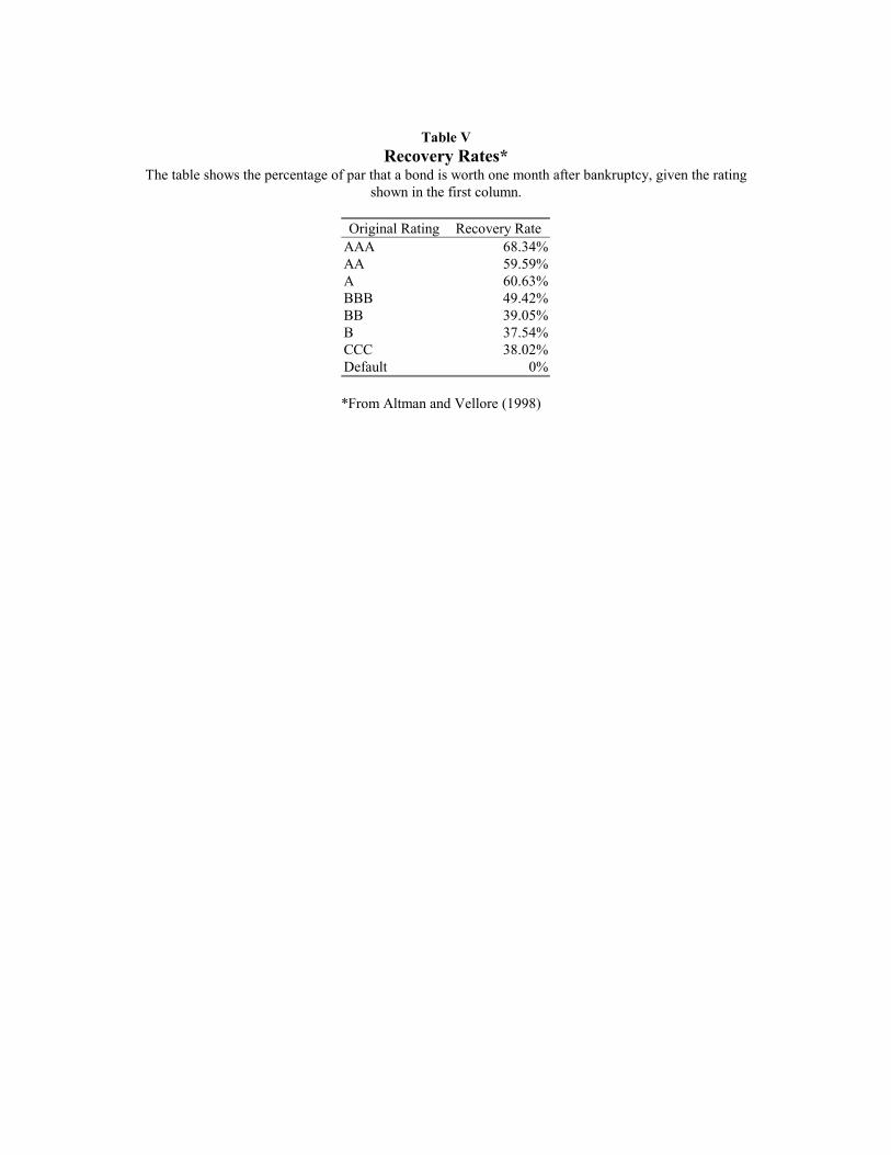
Table VRecovery Rates*

The table shows the percentage of par that a bond is worth one month after bankruptcy, given the ratingshown in the first column.

Original Rating Recovery RateAAA 68.34%AA 59.59%A 60.63%BBB 49.42%BB 39.05%B 37.54%CCC 38.02%Default 0%

*From Altman and Vellore (1998)

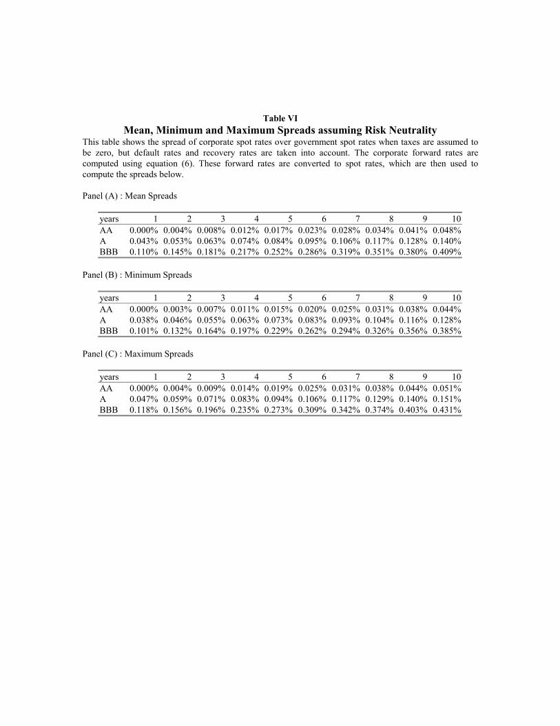
Table VIMean, Minimum and Maximum Spreads assuming Risk Neutrality

This table shows the spread of corporate spot rates over government spot rates when taxes are assumed tobe zero, but default rates and recovery rates are taken into account. The corporate forward rates arecomputed using equation (6). These forward rates are converted to spot rates, which are then used tocompute the spreads below.

Panel (A) : Mean Spreads

years 1 2 3 4 5 6 7 8 9 10AA 0.000% 0.004% 0.008% 0.012% 0.017% 0.023% 0.028% 0.034% 0.041% 0.048%A 0.043% 0.053% 0.063% 0.074% 0.084% 0.095% 0.106% 0.117% 0.128% 0.140%BBB 0.110% 0.145% 0.181% 0.217% 0.252% 0.286% 0.319% 0.351% 0.380% 0.409%

Panel (B) : Minimum Spreads

years 1 2 3 4 5 6 7 8 9 10AA 0.000% 0.003% 0.007% 0.011% 0.015% 0.020% 0.025% 0.031% 0.038% 0.044%A 0.038% 0.046% 0.055% 0.063% 0.073% 0.083% 0.093% 0.104% 0.116% 0.128%BBB 0.101% 0.132% 0.164% 0.197% 0.229% 0.262% 0.294% 0.326% 0.356% 0.385%

Panel (C) : Maximum Spreads

years 1 2 3 4 5 6 7 8 9 10AA 0.000% 0.004% 0.009% 0.014% 0.019% 0.025% 0.031% 0.038% 0.044% 0.051%A 0.047% 0.059% 0.071% 0.083% 0.094% 0.106% 0.117% 0.129% 0.140% 0.151%BBB 0.118% 0.156% 0.196% 0.235% 0.273% 0.309% 0.342% 0.374% 0.403% 0.431%

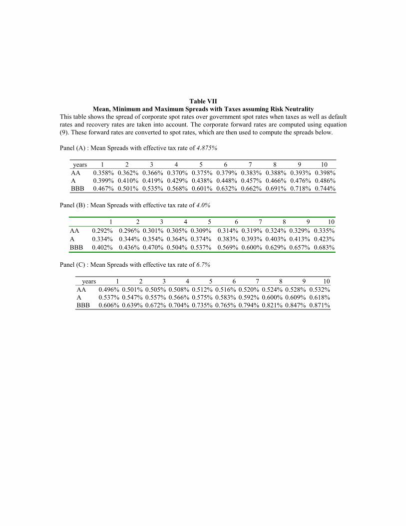
Table VIIMean, Minimum and Maximum Spreads with Taxes assuming Risk Neutrality

This table shows the spread of corporate spot rates over government spot rates when taxes as well as defaultrates and recovery rates are taken into account. The corporate forward rates are computed using equation(9). These forward rates are converted to spot rates, which are then used to compute the spreads below.

Panel (A) : Mean Spreads with effective tax rate of 4.875%

years 1 2 3 4 5 6 7 8 9 10AA 0.358% 0.362% 0.366% 0.370% 0.375% 0.379% 0.383% 0.388% 0.393% 0.398%A 0.399% 0.410% 0.419% 0.429% 0.438% 0.448% 0.457% 0.466% 0.476% 0.486%BBB 0.467% 0.501% 0.535% 0.568% 0.601% 0.632% 0.662% 0.691% 0.718% 0.744%

Panel (B) : Mean Spreads with effective tax rate of 4.0%

1 2 3 4 5 6 7 8 9 10AA 0.292% 0.296% 0.301% 0.305% 0.309% 0.314% 0.319% 0.324% 0.329% 0.335%A 0.334% 0.344% 0.354% 0.364% 0.374% 0.383% 0.393% 0.403% 0.413% 0.423%BBB 0.402% 0.436% 0.470% 0.504% 0.537% 0.569% 0.600% 0.629% 0.657% 0.683%

Panel (C) : Mean Spreads with effective tax rate of 6.7%

years 1 2 3 4 5 6 7 8 9 10AA 0.496% 0.501% 0.505% 0.508% 0.512% 0.516% 0.520% 0.524% 0.528% 0.532%A 0.537% 0.547% 0.557% 0.566% 0.575% 0.583% 0.592% 0.600% 0.609% 0.618%BBB 0.606% 0.639% 0.672% 0.704% 0.735% 0.765% 0.794% 0.821% 0.847% 0.871%

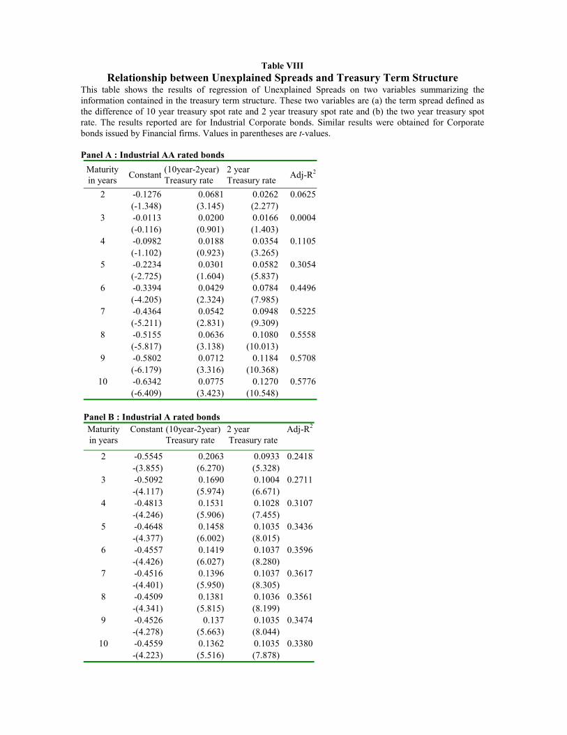
Table VIIIRelationship between Unexplained Spreads and Treasury Term Structure

This table shows the results of regression of Unexplained Spreads on two variables summarizing theinformation contained in the treasury term structure. These two variables are (a) the term spread defined asthe difference of 10 year treasury spot rate and 2 year treasury spot rate and (b) the two year treasury spotrate. The results reported are for Industrial Corporate bonds. Similar results were obtained for Corporatebonds issued by Financial firms. Values in parentheses are t-values.

Panel A : Industrial AA rated bonds

Maturityin years

Constant(10year-2year)Treasury rate

2 yearTreasury rate

Adj-R2

2 -0.1276 0.0681 0.0262 0.0625(-1.348) (3.145) (2.277)

3 -0.0113 0.0200 0.0166 0.0004(-0.116) (0.901) (1.403)

4 -0.0982 0.0188 0.0354 0.1105(-1.102) (0.923) (3.265)

5 -0.2234 0.0301 0.0582 0.3054(-2.725) (1.604) (5.837)

6 -0.3394 0.0429 0.0784 0.4496(-4.205) (2.324) (7.985)

7 -0.4364 0.0542 0.0948 0.5225(-5.211) (2.831) (9.309)

8 -0.5155 0.0636 0.1080 0.5558(-5.817) (3.138) (10.013)

9 -0.5802 0.0712 0.1184 0.5708(-6.179) (3.316) (10.368)

10 -0.6342 0.0775 0.1270 0.5776(-6.409) (3.423) (10.548)

Panel B : Industrial A rated bondsMaturityin years

Constant (10year-2year)Treasury rate

2 yearTreasury rate

Adj-R2

2 -0.5545 0.2063 0.0933 0.2418-(3.855) (6.270) (5.328)

3 -0.5092 0.1690 0.1004 0.2711-(4.117) (5.974) (6.671)

4 -0.4813 0.1531 0.1028 0.3107-(4.246) (5.906) (7.455)

5 -0.4648 0.1458 0.1035 0.3436-(4.377) (6.002) (8.015)

6 -0.4557 0.1419 0.1037 0.3596-(4.426) (6.027) (8.280)

7 -0.4516 0.1396 0.1037 0.3617-(4.401) (5.950) (8.305)

8 -0.4509 0.1381 0.1036 0.3561-(4.341) (5.815) (8.199)

9 -0.4526 0.137 0.1035 0.3474-(4.278) (5.663) (8.044)

10 -0.4559 0.1362 0.1035 0.3380-(4.223) (5.516) (7.878)

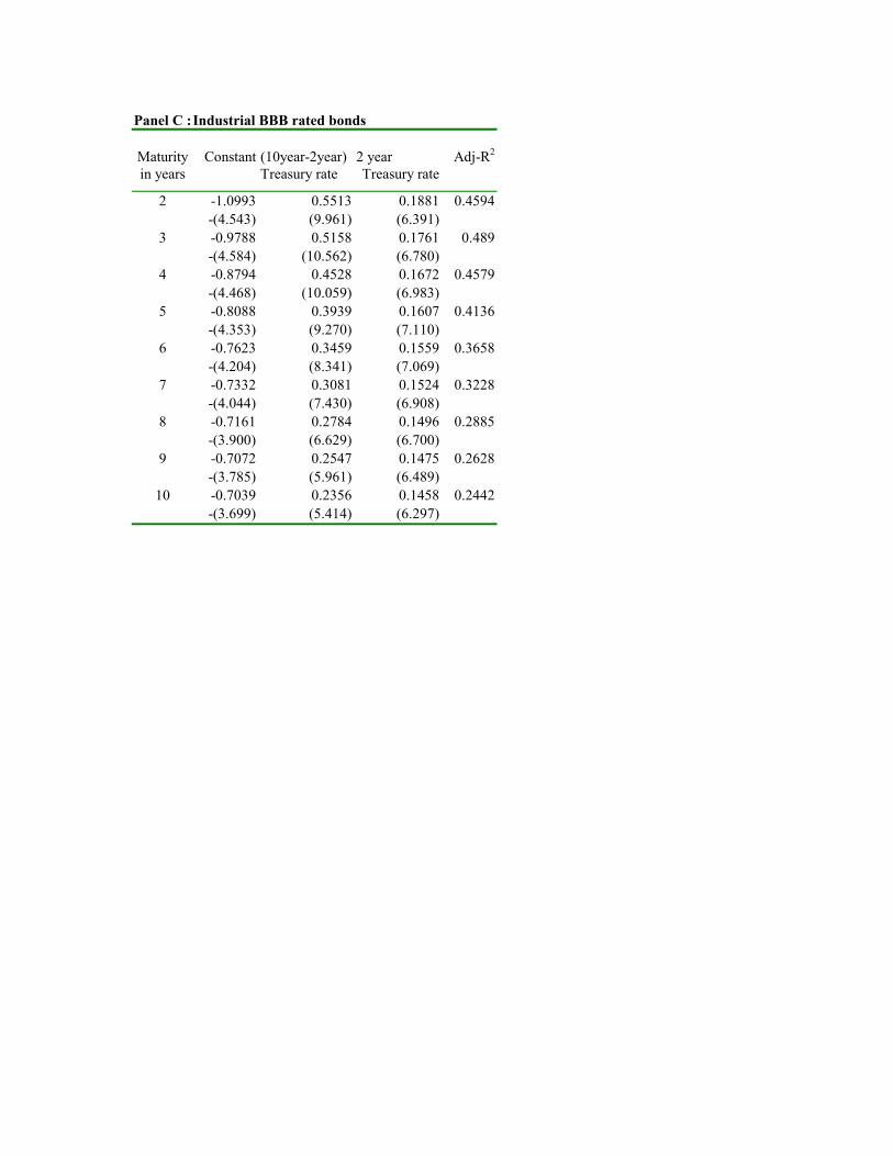
Panel C :Industrial BBB rated bonds

Maturityin years

Constant (10year-2year)Treasury rate

2 yearTreasury rate

Adj-R2

2 -1.0993 0.5513 0.1881 0.4594-(4.543) (9.961) (6.391)

3 -0.9788 0.5158 0.1761 0.489-(4.584) (10.562) (6.780)

4 -0.8794 0.4528 0.1672 0.4579-(4.468) (10.059) (6.983)

5 -0.8088 0.3939 0.1607 0.4136-(4.353) (9.270) (7.110)

6 -0.7623 0.3459 0.1559 0.3658-(4.204) (8.341) (7.069)

7 -0.7332 0.3081 0.1524 0.3228-(4.044) (7.430) (6.908)

8 -0.7161 0.2784 0.1496 0.2885-(3.900) (6.629) (6.700)

9 -0.7072 0.2547 0.1475 0.2628-(3.785) (5.961) (6.489)

10 -0.7039 0.2356 0.1458 0.2442-(3.699) (5.414) (6.297)

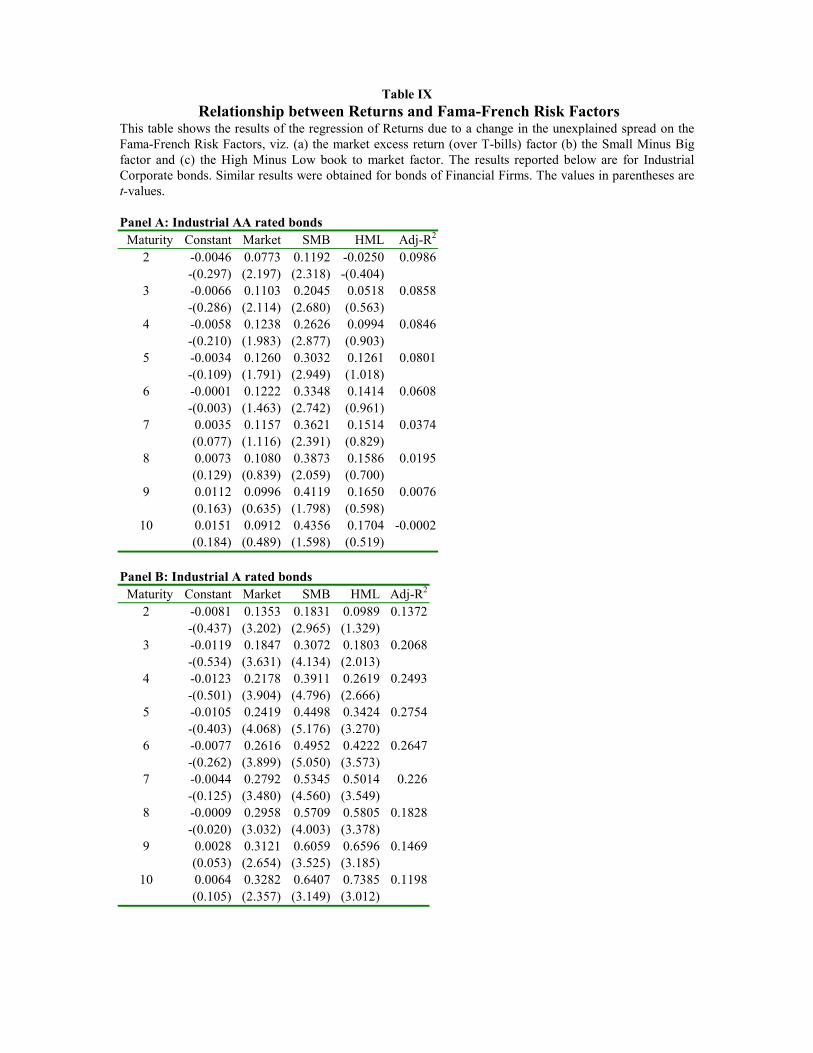
Table IX Relationship between Returns and Fama-French Risk Factors

This table shows the results of the regression of Returns due to a change in the unexplained spread on theFama-French Risk Factors, viz. (a) the market excess return (over T-bills) factor (b) the Small Minus Bigfactor and (c) the High Minus Low book to market factor. The results reported below are for IndustrialCorporate bonds. Similar results were obtained for bonds of Financial Firms. The values in parentheses aret-values.

Panel A: Industrial AA rated bondsMaturity Constant Market SMB HML Adj-R2

2 -0.0046 0.0773 0.1192 -0.0250 0.0986-(0.297) (2.197) (2.318) -(0.404)

3 -0.0066 0.1103 0.2045 0.0518 0.0858-(0.286) (2.114) (2.680) (0.563)

4 -0.0058 0.1238 0.2626 0.0994 0.0846-(0.210) (1.983) (2.877) (0.903)

5 -0.0034 0.1260 0.3032 0.1261 0.0801-(0.109) (1.791) (2.949) (1.018)

6 -0.0001 0.1222 0.3348 0.1414 0.0608-(0.003) (1.463) (2.742) (0.961)

7 0.0035 0.1157 0.3621 0.1514 0.0374(0.077) (1.116) (2.391) (0.829)

8 0.0073 0.1080 0.3873 0.1586 0.0195(0.129) (0.839) (2.059) (0.700)

9 0.0112 0.0996 0.4119 0.1650 0.0076(0.163) (0.635) (1.798) (0.598)

10 0.0151 0.0912 0.4356 0.1704 -0.0002(0.184) (0.489) (1.598) (0.519)

Panel B: Industrial A rated bondsMaturity Constant Market SMB HML Adj-R2

2 -0.0081 0.1353 0.1831 0.0989 0.1372-(0.437) (3.202) (2.965) (1.329)

3 -0.0119 0.1847 0.3072 0.1803 0.2068-(0.534) (3.631) (4.134) (2.013)

4 -0.0123 0.2178 0.3911 0.2619 0.2493-(0.501) (3.904) (4.796) (2.666)

5 -0.0105 0.2419 0.4498 0.3424 0.2754-(0.403) (4.068) (5.176) (3.270)

6 -0.0077 0.2616 0.4952 0.4222 0.2647-(0.262) (3.899) (5.050) (3.573)

7 -0.0044 0.2792 0.5345 0.5014 0.226-(0.125) (3.480) (4.560) (3.549)

8 -0.0009 0.2958 0.5709 0.5805 0.1828-(0.020) (3.032) (4.003) (3.378)

9 0.0028 0.3121 0.6059 0.6596 0.1469(0.053) (2.654) (3.525) (3.185)

10 0.0064 0.3282 0.6407 0.7385 0.1198(0.105) (2.357) (3.149) (3.012)

Panel C: Industrial BBB rated bondsMaturity Constant Market SMB HML Adj-R2

2 0.0083 0.1112 0.3401 0.1259 0.0969(0.276) (1.626) (3.403) (1.045)

3 0.0094 0.1691 0.4656 0.2922 0.1263(0.255) (2.010) (3.787) (1.972)

4 0.0084 0.2379 0.5836 0.4605 0.1798(0.209) (2.601) (4.365) (2.858)

5 0.0062 0.3132 0.6987 0.6263 0.2585(0.153) (3.406) (5.199) (3.867)

6 0.0034 0.3919 0.8127 0.7901 0.3126(0.080) (4.025) (5.711) (4.607)

7 0.0004 0.4720 0.9260 0.9522 0.3122(0.008) (4.147) (5.567) (4.750)

8 -0.0028 0.5528 1.0395 1.1139 0.2807-(0.045) (3.951) (5.084) (4.520)

9 -0.006 0.6341 1.1529 1.2754 0.2445-(0.079) (3.685) (4.585) (4.209)

10 -0.0092 0.7154 1.2662 1.4370 0.2136-(0.101) (3.446) (4.173) (3.930)

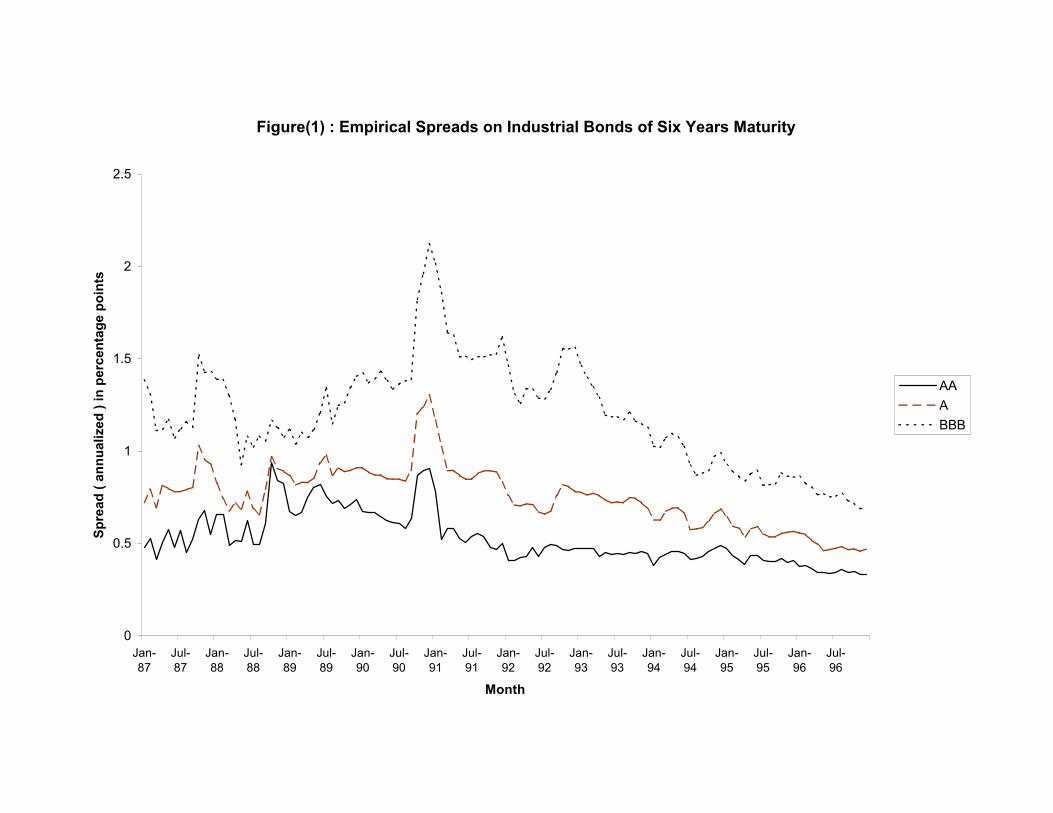
Figure(1) : Empirical Spreads on Industrial Bonds of Six Years Maturity

0

0.5

1

1.5

2

2.5

Jan-87

Jul-87

Jan-88

Jul-88

Jan-89

Jul-89

Jan-90

Jul-90

Jan-91

Jul-91

Jan-92

Jul-92

Jan-93

Jul-93

Jan-94

Jul-94

Jan-95

Jul-95

Jan-96

Jul-96

Month

Sp

read

( a

nn

ual

ized

) i

n p

erce

nta

ge

po

ints

AA

A

BBB

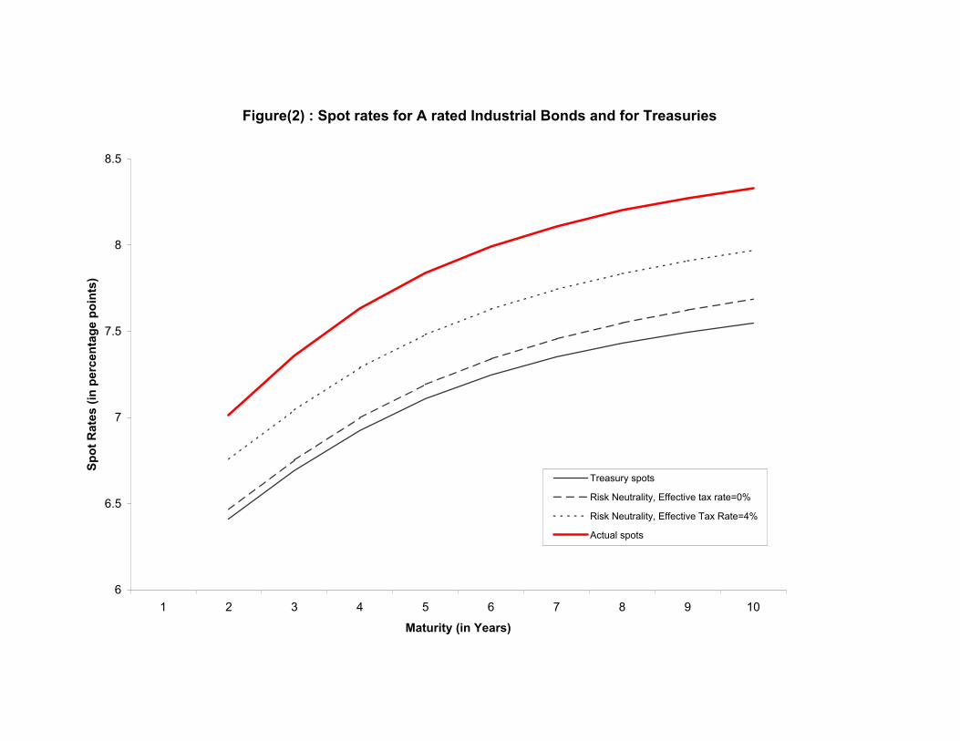
Figure(2) : Spot rates for A rated Industrial Bonds and for Treasuries

6

6.5

7

7.5

8

8.5

1 2 3 4 5 6 7 8 9 10

Maturity (in Years)

Sp

ot

Rat

es (

in p

erce

nta

ge

po

ints

)

Treasury spots

Risk Neutrality, Effective tax rate=0%

Risk Neutrality, Effective Tax Rate=4%

Actual spots

25

REFERENCES

Altman, Edward, 1997, Rating migration of corporate bonds: Comparative results and investor/lenderimplications, NYU Salomon Center Working Paper Series S-97-3.

Altman, Edward, 1989, Measuring corporate bond mortality and performance, Journal of Finance44, 909-922.

Altman, Edward and Kishore Vellore, 1998, Defaults and returns on high yield bonds: Analysis through1997. NYU Salomon Center Working Paper Series S-98-1.

Black, F. and M. Scholes, 1983, The pricing of options and corporate liabilities, Journal of PoliticalEconomy 81, 399-418.

Blume, M. E., D.B. Keim and S.A. Patel, 1991, Returns and the volatility of low grade bonds, Journalof Finance 46, 49-74.

Bodie, Zvi, Kane, Alex, and Marcus, Alan, 1993, Investments, Irwin, Homewood, Illinois.

Brown, K., W. Harlow and D. Smith, 1993, An empirical analysis of interest rate swap spreads, Journal of Fixed Income, 3 March, 61-78.

Cathcart, L. and L. El-Jahel, 1998, Valuation of defaultable bonds, Journal of Fixed Income, 8, 65-78.

Carty, L. and J. Fons, 1994, Measuring changes in credit quality, Journal of Fixed Income 4, 27-41.

Chen, N., R. Roll and S. Ross, 1986, Economic factors and the stock market,. Journal of Business59, 383-403.

Commerce Clearing House, 1997. State Tax Handbook. Commerce Clearing House, Inc., Chicago,IL.

Connor, G. and R.A. Korajczyk, 1993, “A test for the Number of Factors in an Approximate FactorModel, Journal of Finance, 48(4), 1263-91

Cornell, B. and R. Green, 1991, Returns and volatility of low-grade bonds, 1977-1989, Journal of Finance 46, 29-48.

Cox, John, Indgersoll, John, and Ross, Steve, 1985, “A Theory of the Term Structure of Interest

26

Rates,” Econometrica, vol 53, pgs. 385-408

Cumby, Bob and Martin Evans, 1995, The term structure of credit risk: estimates and specificationtests, Department of Economics, Georgetown University.

Dahlquist, M. and L.E.O. Svensson. 1996, “Estimating the Term Structure of Interest Rates forMonetary Policy Analysis,” Scadinavian Journal of Economics, 98(2), 163-83

Das, Sanjiv R. and Peter Tufano, 1996, “Pricing Credit Sensitive Debt When Interest Rates, CreditRatings and Credit Spreads are Stochastic,” Journal of Financial Engineering, vol 5, 161-198.

Duffee, G., 1998, “The Relation Between Treasury Yields and Corporate Bond Yield Spreads,” Journal of Finance, vol 53, No 6, pgs 2225-2240.

Duffie, D. and M. Huang, 1994, Swap rates and credit quality, Working Paper, Graduate School ofBusiness, Stanford University.

Duffie, D. and K. Singleton, 1997, Modeling term structures of defaultable bonds, Graduate School ofBusiness, Stanford University.

Elton, Edwin, and T. Clifton Green, 1998, “Tax and Liquidity Effects in Pricing Government Bonds,”Journal of Finance, vol 53, No.5, pgs. 1533-1562.

Elton, E., M. Gruber and Blake, C., 1998, Common factors in mutual fund returns, Forthcoming, European Finance Review.

Elton, Edwin J., M. Gruber and R. Michaely, 1990, “The Structure of Spot Rates and Immunization,”Journal of Finance.

Fama, E.F., 1986, Term premiums and default premiums in money markets, Journal of FinancialEconomics 17, 175-196.

Fama, E. and K. French, 1993, Common risk factors in the returns on stocks and bonds, Journal ofFinancial Economics 33, 3-57.

Fisher, L., 1959, Determinants of risk premiums on corporate bonds, Journal of Political Economy67, 217-237.

27

Fons, Jerome S., 1994, Using default rates to model the term structure of credit risk, FinancialAnalysts Journal 50, 25-32.

Geske, R., 1977, The valuation of corporate liabilities as compound options, Journal of Financial andQuantitative Analysis 12, 541-552.

Goodman, L.S., 1989, High yield default rates: is there cause for concern?, Goldman, Sachs & Co.,Fixed Income Research, New York.

Green, C. and A. Odegaard, 1997, Tax effects in relative pricing of U.S. government bonds, Journal of Finance 52, 2, 609-633.

Helwege, J. and P. Kleinan, 1997, Understanding aggregate default rates of high yield bonds, Journal of Fixed Income 7, 55-61.

Helwege, J. and C. Turner, 1996, The slope of the credit yield curve for speculative grade issues,Unpublished working paper, Federal Reserve Bank of New York.

Jarrow, R. A. Lando, and S. Turnbull, 1994, A Markov model for the term structure of credit spreads,Review Of Financial Studies, vol 10 pp 481-523.

Johnson, R., 1967, Term structure of corporate bonds yields as a function of risk of default, Journal of Finance 22, 313-345.

Kim, I., K. Ramaswamy and S. Sundaresan, 1987,. The valuation of corporate fixed incomesecurities,. Manuscript, Columbia University.

Lando, D., 1994, On Cox processes and credit risky bonds, Working paper, Institute of MathematicalStatistics, University of Copenhagen, Denmark.

Litterman, R. and J. Scheinkman, 1991, Common factors affecting bond returns, Journal of FixedIncome 1, 54-61.

Litzenberger, H. and Rolfo, 1984, An international study of tax effects on government bond prices,Journal of Finance 39, 1-22.

Longstaff, F.A. and E.S. Schwartz, 1995, A simple approach to valuing risky fixed and floating ratedebt, Journal of Finance 50, 789-819.

Madan, D. B. and H. Unal, 1994, Pricing the risks of default, Working paper, Wharton School,

28

University of Pennsylvania.

Mason, S.P. and S. Bhattacharya, 1981, Risky debt, jump process, and safety covenants, Journal ofFinancial Economics 9, 281-307.

McCulloch, J., 1971, “Measuring the Term Structure of Interest Rates,” Journal of Business, 44, 19-31.

Merton, R.C., 1974, On the pricing of corporate debt: the risk structure of interest rates, Journal of Finance 29, 449-470.

Moodys Investors Service, 1998, Historical default rates of corporate bond issuers 1920-1997.

Nelson, R. and F. Siegel, 1987, Parsimonious modeling of yield curves, Journal of Business 60, 473-489.

Nielsen, L. J. Saá-Requejo, and P. Santa-Clara, 1993, Default risk and interest rate risk: the termstructure of default spreads, Working Paper, INSEAD, Fontainebleau, France.

Pitts, C.G.C. and M.J.P. Selby, 1983, The pricing of corporate debt: a further note, Journal ofFinance 38, 1311-1313.

Sarig, O. and A. Warga, 1989, Bond price data and bond market liquidity, Journal of Financial andQuantitative Analysis 24, 367-378.

Sarig, O. and A. Warga, 1989, Some empirical estimates of the risk structure of interest rates, Journal of Finance 44, 1351-1360.

Severn, A. K. and W. J. Stewart, 1992, The corporate-Treasury yield spread and state taxes, Journal of Economics and Business 44, 161-166.

Warga, A., 1998, Fixed income data base, University of Houston, Houston, Texas

WWei, D. G. and G. Dajiang, 1997, Pricing risky debt: an empirical comparison of the Longstaff andSchwartz and Merton models, Journal of Fixed Income 7, 8-28.