On the usefulness of cross-validationfor directional forecast evaluation

Christoph Bergmeir1, Mauro Costantini2, and JoseM. Benıtez1∗

1Department of Computer Science and Artificial Intelligence,E.T.S. de Ingenierıas Informatica y de Telecomunicacion,

University of Granada, Spain.2Department of Economics and Finance, Brunel University,

United Kingdom

Abstract

The usefulness of a predictor evaluation framework which combinesa blocked cross-validation scheme with directional accuracy measuresis investigated. The advantage of using a blocked cross-validationscheme with respect to the standard out-of-sample procedure is thatcross-validation yields more precise error estimates of the predictionerror since it makes full use of the data. In order to quantify the gain inprecision when directional accuracy measures are considered, a MonteCarlo analysis using univariate and multivariate models is provided.The experiments indicate that more precise estimates are obtainedwith the blocked cross-validation procedure. An application is car-ried out on forecasting UK interest rate for illustration purposes. Theresults show that in such a situation with small samples the cross-validation scheme may have considerable advantages over the stan-dard out-of-sample evaluation procedure as it may help to overcomeproblems induced by the limited information the directional accuracymeasures contain due to their binary nature.

KEY WORDS Blocked cross-validation; out-of-sample evaluation; forecastdirectional accuracy; Monte Carlo analysis; linear models.

∗Corresponding author. DECSAI, ETSIIT, UGR, C/ Periodista Daniel SaucedoAranda s/n, 18071 - Granada, Spain, E-mail address: j.m.benitez@decsai.ugr.es

1 Introduction

Assessing and evaluating the accuracy of forecasting models and forecasts isan important and long-standing problem which a forecaster always faces whenchoosing among various available forecasting methods. This paper aims toinvestigate the usefulness of a blocked cross-validation (BCV) scheme alongwith directional accuracy measures for forecast evaluation. Several forecasterror measures such as scale-dependent, percentage and relative measureshave been used largely for forecast evaluation (see Hyndman and Koehler(2006); Costantini and Pappalardo (2010), Costantini and Kunst (2011)among others).

However, Blaskowitz and Herwartz (2009) point out that directional fore-casts can provide a useful framework for assessing the economic forecast valuewhen loss functions (or success measures) are properly formulated to accountfor the realized signs and realized magnitudes of directional movements. Inthis regard, Blaskowitz and Herwartz (2009, 2011) propose several directionalaccuracy measures which assign a different loss to the forecast, depending onwhether it correctly predicts the direction (rise/fall) of the time series or not.The idea behind this kind of measure is that there are many situations wherethe correct prediction of the direction of the time series can be very useful,even if the forecast is biased (an investor buys stock, if its price is expectedto rise, Blaskowitz and Herwartz (2009); a central bank tends to increase theinterest rate, if inflation is expected to rise, Milas and Naraidoo (2012)).For purposes of out-of-sample (OOS) forecast evaluation, the sample is di-vided into two parts. A fraction of the sample is reserved for initial parameterestimation while the remaining fraction is used for evaluation. However, thisprocedure may fail to work well when the overall amount of data is limitedand/or a lot of parameters are to be estimated. As the directional accuracymeasures use the predictions in a binary way (correct/incorrect prediction ofdirection), the problems may be even more prominent when using such mea-sures. Provided that the data used for forecasting are stationary (see Arlotand Celisse (2010)), the cross-validation scheme may help improve the esti-mation of the forecast directional accuracy, as it uses the data more efficientlyby splitting them into k-folds. In this context, the use of the directional fore-casting accuracy is also recommended since changes in the sign are frequentwith stationary data (no increasing/decreasing trend).This paper makes a contribution to the existing literature by investigat-ing whether, and to what extent, the k-fold BCV procedure proposed byBergmeir and Benıtez (2012) may provide a better estimate of forecast di-rectional accuracy than the standard OOS procedure. The use of the k-foldblocked scheme is suggested because it yields more precise error measures, in

2

the sense that the error measure calculated using BCV is a better estimate ofthe generalization error (the expected loss of the model on unknown futureobservations; see Blum et al. (1999); Hastie et al. (2009)).

This paper aims to evaluate if this benefit is also retained when the fore-casts are tested for directional accuracy. To this end, we provide a MonteCarlo analysis using simple univariate and multivariate linear autoregressivemodels. The models are estimated and evaluated both with BCV and tradi-tional OOS evaluation methods. Furthermore, the models are also evaluatedon an additional validation set which consists of new unknown future data.This allows us to compare the directional accuracy obtained by the evalua-tion procedure and the directional accuracy obtained using the new futuredata. In this way, it is possible to ascertain how well the evaluation proce-dure is able to predict the future loss of a certain model. The Monte Carloexperiment results show that the advantage of using a BCV scheme is quiteremarkable.

We use simple linear models as these models are likely to show a ratherconservative behavior compared to more complex models regarding the dif-ferences in the outcome of the forecast evaluation, as more complex modelsrequire more data for parameter estimation, so the observed effects may beeven stronger with complex models. Also, autoregressive models have beenextensively used in the literature for directional forecasts, especially for theprediction of the exchange rate and the interest rate, as it is of primaryimportance for investors and policy makers to better understand the move-ments of these variables for the decision-making process (see Kong (2000);Sosvilla-Rivero and Garcıa (2005); Kim et al. (2008); Blaskowitz and Her-wartz (2014); Blaskowitz and Herwartz (2009); Altavilla and De Grauwe(2010), among others). The use of these models has been justified on thebasis of the potential correlation in the change of the exchange rate due todata measurement or aggregation (see Kong (2000)) and in the interest ratedue to monetary policy of the central bank.

We also offer an empirical application to the UK interest rate data. Theforecast results show that, when using directional accuracy measures in smallsample sizes, it may happen that distinct forecast approaches reveal identicalrealized average loss/success. The BCV scheme uses additional informationfrom other test sets and is less likely to obtain identical loss estimates, thusit is able to distinguish the performance of the models.

The rest of the paper is organized as follows. Section 2 reviews the BCVprocedure. Section 3 describes the directional accuracy measures. Section 4provides the Monte Carlo results. Section 5 discusses our empirical findings,and Section 6 concludes.

3

2 Blocked cross-validation

Cross-validation is an estimator widely used to evaluate prediction errors(Borra and Di Ciaccio, 2010; Khan et al., 2010). In k-fold cross-validation(see, e.g., Hastie et al. (2009)), the overall available data is randomly parti-tioned into k sets of equal size: each of the k sets is used once to measure theOOS forecast accuracy and the other k− 1 sets are used to build the model.The k resulting error measures are averaged using the mean to calculate thefinal error measure. The advantage of cross-validation is that all the data isused both for training (initial estimation) and testing and the error measurecan be computed k times instead of only one. Therefore, by averaging overthe k measures, the error estimate using cross-validation has a lower variancecompared to an error estimate using only one training and test set. In thisway, a more accurate evaluation of the generalization error can be obtained(see Blum et al. (1999) for a theoretic result on this).

Since the cross-validation scheme requires the data to be i.i.d. (see Arlotand Celisse (2010)), modified versions of cross-validation for time series anal-ysis have been proposed (for a large survey see Bergmeir and Benıtez (2012)).Identical distribution translates to stationarity of the series (Racine, 2000).Independence can be assured by leaving a margin of a certain distance intime d between training and test values, after which the values are approx-imately independent (and no autocorrelation is present). The value d willbe typically related to the order of the model, as we assume that all theautocorrelation is considered during model building. Therefore, the valuesin a neighborhood of d, around a value which is used for testing, cannot beused for training (see, e.g., McQuarrie and Tsai (1998) or Kunst (2008) forthe procedure).

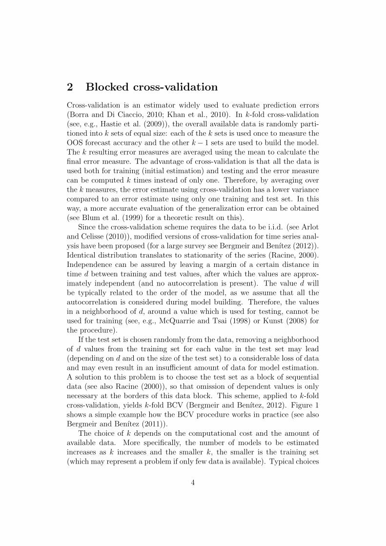
If the test set is chosen randomly from the data, removing a neighborhoodof d values from the training set for each value in the test set may lead(depending on d and on the size of the test set) to a considerable loss of dataand may even result in an insufficient amount of data for model estimation.A solution to this problem is to choose the test set as a block of sequentialdata (see also Racine (2000)), so that omission of dependent values is onlynecessary at the borders of this data block. This scheme, applied to k-foldcross-validation, yields k-fold BCV (Bergmeir and Benıtez, 2012). Figure 1shows a simple example how the BCV procedure works in practice (see alsoBergmeir and Benıtez (2011)).

The choice of k depends on the computational cost and the amount ofavailable data. More specifically, the number of models to be estimatedincreases as k increases and the smaller k, the smaller is the training set(which may represent a problem if only few data is available). Typical choices

4

5-fold blocked cross-validation

out-of-sample evaluation

Figure 1: Training and test sets chosen for traditional OOS evaluation, and 5-fold BCV.Blue dots represent points from the time series in the training set and orange dots representpoints in the test set. In the example, we assume that the model uses two lagged valuesfor forecasting, which is why at the borders always two values are omitted.

for k are 5 or 10 (see Khan et al. (2010); Hastie et al. (2009)). In this workwe use k = 5.

In the following, we offer a theoretical analysis to show the advantageof using BCV over OOS. Specifically, we will show that the BCV procedureyields an error measure with a lower variance than that of OOS.

Let xt be a time series. Let D be a (N, p + 1)-matrix of time seriesdata to which an autoregressive model is applied. The rows of D are ofthe form ((xt−p), . . . , xt−1, xt, xt+h), where h is the forecast horizon. Letκ : {1, . . . , N} 7→ {1, . . . , k} be an index function that indicates the partitionto which row i belongs to. The index function is built according to theparadigm of BCV, so that k blocks of equal size of data are generated (weassume for simplicity that the length of the time series is a multiple of k).

Let us consider the kth cross-validation estimate, where the kth partitionis used as the test set. Note that this is equivalent to OOS evaluation, usingan OOS period with a length of 1/kth the length of the training data. Weestimate a model f on the data D using all rows i with κ(i) 6= k. Denotesuch a model by f−κk in the following. Then, an error measure M for f−κk

is calculated on D using all rows j with κ(j) = k. We denote such an errormeasure M(f−κk , κk). So, we define the OOS estimate as:

OOS(f) = M(f−κk , κk).

From this, we can straightforwardly define the BCV estimate as:

BCV (f) =1

k

k∑i=1

M(f−κi , κi).

In this case, it is straightforward to see that BCV uses all the informationavailable to OOS and additional information from other test sets. Let us

5

consider the variance of the error measure. Assuming that the error measuresM calculated on different test sets are uncorrelated, we have:

V ar(BCV (f)) = V ar(1

k

k∑i=1

M(f−κi , κi)) =1

k2

k∑i=1

V ar(M(f−κi , κi)),

and for stationary data:

V ar(BCV (f)) =1

k2

k∑i=1

V ar(M(f−κk , κk)) =V ar(OOS(f))

k.

As the BCV estimate has a smaller variance than that of the OOS pro-cedure, for unbiased estimates the BCV procedure yields a more precise es-timate of the generalization error (in the sense of Blum et al. (1999); Hastieet al. (2009)). We investigate this in our Monte Carlo experiments in Sec-tion 4.

However, there are some cases in which the use of the BCV proceduremay not be straightforward, or not be advisable. In the BCV procedure, forall the folds but the first and the last one, the test set interrupts the trainingset, then for some forecasting models (e.g., exponential smoothing methodsor models with a moving average part) it may be difficult to handle trainingsets that consist of two non-continuous parts. Nevertheless, this is not anissue in the broad class of (linear or non-linear) pure autoregressive modelsof fixed order, as in the embedded form of the series only the respective rowshave to be removed before estimating the model.

Also, the use of the BCV procedure is not straightforward when onlythe forecasts, but not the forecasting models, are available, as it then maynot be possible to generate forecasts for the different test sets. This maybe the case when one evaluates the forecasting record of an internationalorganization (e.g. IMF, EC or OECD).

Finally, the use of BCV may also not be recommended when changesat a certain point in time (structural breaks) are present in the data. Inthis respect, it may be counterproductive to use data before the break as itdoes not provide valuable information for future values of the series, both formodel estimation and evaluation.

All in all, the use of BCV is beneficial in the following cases. First, themodel allows for non-continuous training periods. Second, the forecastercontrols the model building steps and can produce the forecasts. Finally, fulluse of the data can be made. In many applications, this is the case, especiallywhen the performance of (linear or non-linear) autoregressive models forstationary data is to be evaluated.

6

3 Directional accuracy measures

Conventional measures of forecasting accuracy are based on the idea of aquadratic loss function in that larger errors carry proportionally greaterweights than smaller ones. Such measures respect the view that forecastevaluation should concentrate on all large disturbances whether or not theyare associated with directional errors which are of no special interest in and ofthemselves. However, several studies argue that incorrectly predicted direc-tions are among the most serious errors a forecast can make (see Chung andHong (2007); Kim et al. (2008); Solferino and Waldmann (2010), Blaskowitzand Herwartz (2009, 2011) among others). In this respect, this study appliessome directional accuracy measures (Blaskowitz and Herwartz (2009, 2011))for forecast evaluation.Using the indicator function I[. . .], the realized and predicted directions Rt

and Pt are given by:

Rt = I [(yt+h − yt) > 0] ,

Pt = I [(yt+h − yt) > 0] ,

where yt is the current value of the series, yt+h is the value of the forecast,and yt+h is the true value of the series at time t+ h.

Using Rt and Pt, the directional error (DE) for h-step-ahead forecasts canbe defined as follows:

DEt = I[Rt = Pt].

Using DE, a general framework for the directional accuracy (DA) can beobtained:

DAt =

{a for DEt = 1b for DEt = 0

In this framework, a correct prediction of the direction takes a value a,which can be interpreted as a reward, and an incorrect prediction takes avalue b, a penalty. Based on the DA, several directional accuracy measurescan be defined.The mean directional accuracy (MDA) is defined straightforwardly as themean of the DA:

MDA = mean(DAt).

7

This measure acquires well the degree up to which the predictor is ableto correctly predict the direction of the forecast, and it is robust to outliers.It should be noted that the following holds:

MDA = (a− b) mean(DEt) + b,

so that MDA is a linear transformation of the mean of the DE, dependingon a and b (this linear relationship can be derived from a contingency tableof sums of correct/incorrect upward/downward predictions). As MDA doesnot take into account the actual size of the change, it does not measure theeconomic value of the forecast (the predictor can be able to forecast the di-rection in cases of low volatility quite well, but it can fail when the volatilityis high). Therefore, we use the directional forecast value (DV), which multi-plies DA by the absolute value of the real changes, thus assessing better theactual benefit/loss of a correct/incorrect direction of the prediction.The mean DV (MDV) is defined as:

MDV = mean(|yt+h − yt| ·DAt).

In order to have a scale-free measure, the absolute value of the changecan be divided by the current value of the series (Blaskowitz and Herwartz,2011). Then, the mean directional forecast percentage value (MDPV) canbe defined as follows:

MDPV = mean

( ∣∣∣∣yt+h − ytyt

∣∣∣∣ ·DAt

).

According to Blaskowitz and Herwartz (2011), common values for a and bare (a, b) = (1, 0), or (a, b) = (1,−1). In the first case, DAt is identical to DEt.In the second case, b is actually a penalty. In our study, we use (a, b) = (1,−1)to consider the more general case where penalties are involved.

4 Monte Carlo experiment

In this section, we provide a Monte Carlo analysis. We consider univariateand multivariate experiments. In the univariate experiment, we generateseries from a stable AR(3) process, while in the multivariate experiments thedata is generated from bivariate and trivariate VAR(2) models, respectively.The design of the first two experiments (univariate case and bivariate VAR(2)model) is stochastic, in the sense that for every Monte Carlo trial the modelparameters are generated randomly and, as a result, we obtain different data

8

for every trial. The third experiment (trivariate VAR(2) model) is designedin line with the empirical application.

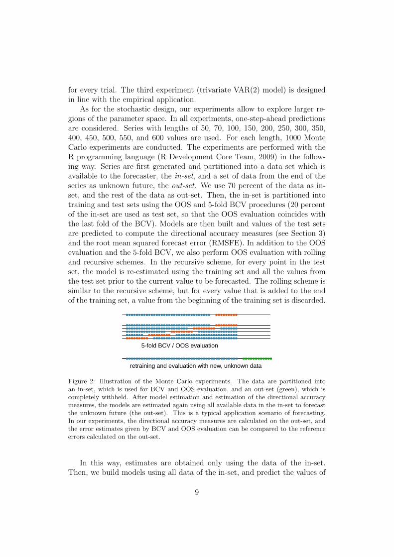
As for the stochastic design, our experiments allow to explore larger re-gions of the parameter space. In all experiments, one-step-ahead predictionsare considered. Series with lengths of 50, 70, 100, 150, 200, 250, 300, 350,400, 450, 500, 550, and 600 values are used. For each length, 1000 MonteCarlo experiments are conducted. The experiments are performed with theR programming language (R Development Core Team, 2009) in the follow-ing way. Series are first generated and partitioned into a data set which isavailable to the forecaster, the in-set, and a set of data from the end of theseries as unknown future, the out-set. We use 70 percent of the data as in-set, and the rest of the data as out-set. Then, the in-set is partitioned intotraining and test sets using the OOS and 5-fold BCV procedures (20 percentof the in-set are used as test set, so that the OOS evaluation coincides withthe last fold of the BCV). Models are then built and values of the test setsare predicted to compute the directional accuracy measures (see Section 3)and the root mean squared forecast error (RMSFE). In addition to the OOSevaluation and the 5-fold BCV, we also perform OOS evaluation with rollingand recursive schemes. In the recursive scheme, for every point in the testset, the model is re-estimated using the training set and all the values fromthe test set prior to the current value to be forecasted. The rolling scheme issimilar to the recursive scheme, but for every value that is added to the endof the training set, a value from the beginning of the training set is discarded.

5-fold BCV / OOS evaluation

retraining and evaluation with new, unknown data

Figure 2: Illustration of the Monte Carlo experiments. The data are partitioned intoan in-set, which is used for BCV and OOS evaluation, and an out-set (green), which iscompletely withheld. After model estimation and estimation of the directional accuracymeasures, the models are estimated again using all available data in the in-set to forecastthe unknown future (the out-set). This is a typical application scenario of forecasting.In our experiments, the directional accuracy measures are calculated on the out-set, andthe error estimates given by BCV and OOS evaluation can be compared to the referenceerrors calculated on the out-set.

In this way, estimates are obtained only using the data of the in-set.Then, we build models using all data of the in-set, and predict the values of

9

the out-set and calculate the directional accuracy measures on the out-set(see also Figure 2). Thus, for each kind of model we obtain an error estimateusing only the in-set data, and an error measure on future values of the series,the out-set data. This allows us to compare the in-set error estimates usingBCV, OOS, rolling and the recursive scheme, and the out-set errors. To thisend, we calculate the root mean squared error of the in-set estimates withrespect to the out-set errors, and we call this measure the root mean squaredpredictive accuracy error (RMSPAE). It is defined as follows:

RMSPAE =

√√√√ 1

n

n∑i=1

(M out−seti −M in−set

i )2 ,

where n is the number of series, i.e., trials in the Monte Carlo simulation,and M is the accuracy measure in consideration, calculated for one modeland one series. In the case of M in−set, the BCV, OOS, rolling, or recursiveprocedure is used on the in-set, and in the case of M out−set, the data of thein-set are used for training, and the data of the out-set are used for testing.

The RMSPAE is an appropriate measure to compare the performancesof different evaluation procedures. Indeed, the RMSPAE does not assess theperformance of a forecasting model, but it assesses the performance of anevaluation procedure (e.g., BCV) to predict the generalization error for adetermined model, regardless of whether the model performs well or not.

4.1 Univariate case

Series are generated from a stable AR(3) process. Real-valued roots of thecharacteristic polynomial are chosen randomly from a uniform distribution inthe interval [−rmax,−1.1]∪ [1.1, rmax], with rmax=5.0. From these roots, thecoefficients of the AR model are estimated (for a more detailed descriptionof the procedure, see Bergmeir and Benıtez (2012)). The first 100 timeseries observations are discarded to avoid possible initial value effects. Theseries are then normalized to zero mean and unit variance. As percentagemeasures such as the MAPE and the MDPV are heavily skewed when theseries have values close to zero (see e.g. Hyndman and Koehler (2006); thisis also confirmed in unreported preliminary experiments), for each series wesubtract the overall minimum (calculated over all series) from all values toobtain a series of non-negative values, and then we increment all values by1, to achieve a series which only contains values greater 1. In this way, newcoefficients are estimated and a new series is generated for each iteration.

For forecasting purposes, we consider the data generating process, AR(3),

10

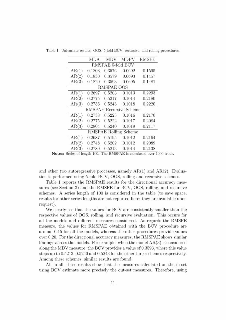
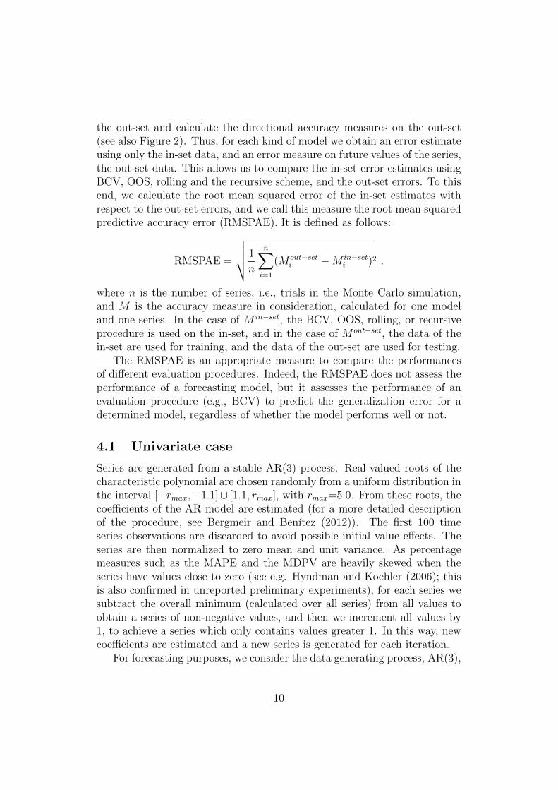
Table 1: Univariate results. OOS, 5-fold BCV, recursive, and rolling procedures.

MDA MDV MDPV RMSFERMSPAE 5-fold BCV

AR(1) 0.1803 0.3576 0.0692 0.1595AR(2) 0.1830 0.3579 0.0693 0.1457AR(3) 0.1820 0.3593 0.0695 0.1481

RMSPAE OOSAR(1) 0.2697 0.5203 0.1013 0.2293AR(2) 0.2775 0.5217 0.1014 0.2180AR(3) 0.2756 0.5243 0.1018 0.2220

RMSPAE Recursive SchemeAR(1) 0.2738 0.5223 0.1016 0.2170AR(2) 0.2775 0.5222 0.1017 0.2084AR(3) 0.2804 0.5240 0.1019 0.2117

RMSPAE Rolling SchemeAR(1) 0.2687 0.5195 0.1012 0.2164AR(2) 0.2748 0.5202 0.1012 0.2089AR(3) 0.2780 0.5213 0.1014 0.2138

Notes: Series of length 100. The RMSPAE is calculated over 1000 trials.

and other two autoregressive processes, namely AR(1) and AR(2). Evalua-tion is performed using 5-fold BCV, OOS, rolling and recursive schemes.

Table 1 reports the RMSPAE results for the directional accuracy mea-sures (see Section 3) and the RMSFE for BCV, OOS, rolling, and recursiveschemes. A series length of 100 is considered in the table (to save space,results for other series lengths are not reported here; they are available uponrequest).

We clearly see that the values for BCV are consistently smaller than therespective values of OOS, rolling, and recursive evaluation. This occurs forall the models and different measures considered. As regards the RMSFEmeasure, the values for RMSPAE obtained with the BCV procedure arearound 0.15 for all the models, whereas the other procedures provide valuesover 0.20. For the directional accuracy measures, the RMSPAE shows similarfindings across the models. For example, when the model AR(3) is consideredalong the MDV measure, the BCV provides a value of 0.3593, where this valuesteps up to 0.5213, 0.5240 and 0.5243 for the other three schemes respectively.Among these schemes, similar results are found.

All in all, these results show that the measures calculated on the in-setusing BCV estimate more precisely the out-set measures. Therefore, using

11

100 200 300 400 500 600

0.0

0.3

MDA

LengthR

MS

PAE

OOSBCV

100 200 300 400 500 600

0.0

0.6

MDV

Length

RM

SPA

E

100 200 300 400 500 6000.00

0.12

MDPV

Length

RM

SPA

E

Figure 3: RMSPAE averaged over the Monte Carlo trials AR(3). Series of different lengths.

BCV, one is able to estimate the directional accuracy for a given methodmore precisely when predicting unknown future values of the series.

Another important result emerges from the experiment. Figure 3 showsthe RMSPAEs for the series of all lengths when an AR(3) model is con-sidered. The results indicate that in general the RMSPAE decreases withincreasing length of the series, so that the directional accuracy is estimatedmore precisely if more data are available. Also, advantages of cross-validationare bigger if the series are shorter which is often the case in empirical appli-cations.

4.2 Multivariate case

For the multivariate case, two studies are performed. The first study is inline with the univariate experiments discussed so far, while the second studyis motivated by our application.

4.2.1 Multivariate experiment with stochastic design

The purpose of this multivariate Monte Carlo simulation study is to verifythe robustness of the results in Section 4.1. The data generating processis a bivariate VAR(2) model. Series are generated in a similar way as inSection 4.1. Eigenvalues for the companion matrix of the VAR model are

12

generated, with an absolute value smaller than 1, in order to obtain a sta-ble model (Lutkepohl, 2006). The companion matrix is generated from theseeigenvalues by the procedure described by Boshnakov and Iqelan (2009). Thecovariance matrix is randomly chosen by generating an upper triangular ma-trix from a uniform distribution in the [−1, 1] interval where the elementson the diagonal are set equal to 1. Therefore, a random symmetric matrixis built up. The random values for the VAR process are then drawn froma Gaussian distribution, and multiplied by the Cholesky form of the covari-ance matrix. As in the univariate experiment, the first 100 observations arediscarded and the resulting series are normalized to have zero mean and unitvariance. Then, the series are shifted to prevent problems with percentagemeasures (by incrementing each value by 1 and subtracting the overall min-imum from the series).

In analogy to the application in Section 5, we use only the first componentof the bivariate model for the evaluation. Along with the VAR(2) model, twoother models are used for forecasting purposes, namely the bivariate VAR(1)and VAR(3) model.

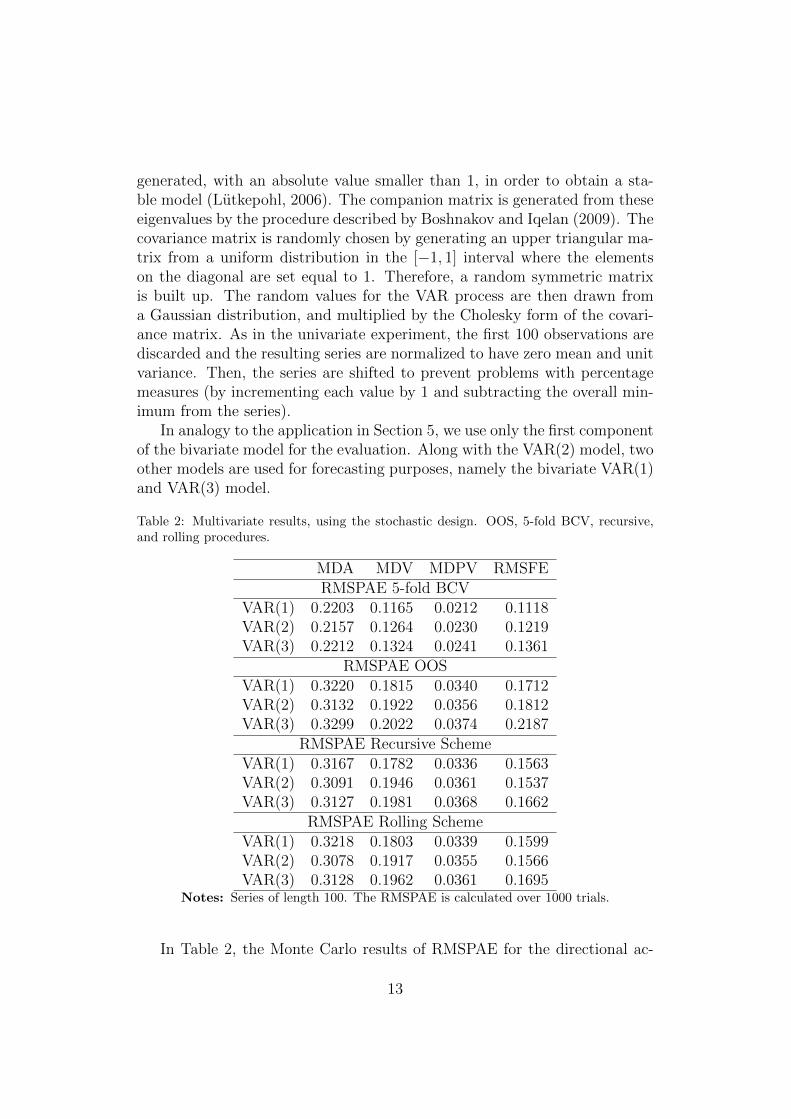
Table 2: Multivariate results, using the stochastic design. OOS, 5-fold BCV, recursive,and rolling procedures.

MDA MDV MDPV RMSFERMSPAE 5-fold BCV

VAR(1) 0.2203 0.1165 0.0212 0.1118VAR(2) 0.2157 0.1264 0.0230 0.1219VAR(3) 0.2212 0.1324 0.0241 0.1361

RMSPAE OOSVAR(1) 0.3220 0.1815 0.0340 0.1712VAR(2) 0.3132 0.1922 0.0356 0.1812VAR(3) 0.3299 0.2022 0.0374 0.2187

RMSPAE Recursive SchemeVAR(1) 0.3167 0.1782 0.0336 0.1563VAR(2) 0.3091 0.1946 0.0361 0.1537VAR(3) 0.3127 0.1981 0.0368 0.1662

RMSPAE Rolling SchemeVAR(1) 0.3218 0.1803 0.0339 0.1599VAR(2) 0.3078 0.1917 0.0355 0.1566VAR(3) 0.3128 0.1962 0.0361 0.1695

Notes: Series of length 100. The RMSPAE is calculated over 1000 trials.

In Table 2, the Monte Carlo results of RMSPAE for the directional ac-

13

100 200 300 400 500 600

0.0

0.3

MDA

LengthR

MS

PAE

OOSBCV

100 200 300 400 500 6000.00

0.25

MDV

Length

RM

SPA

E

100 200 300 400 500 6000.00

0.05

MDPV

Length

RM

SPA

E

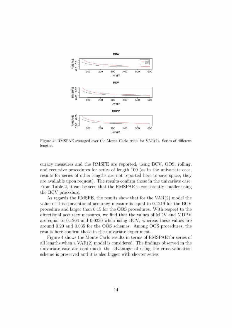
Figure 4: RMSPAE averaged over the Monte Carlo trials for VAR(2). Series of differentlengths.

curacy measures and the RMSFE are reported, using BCV, OOS, rolling,and recursive procedures for series of length 100 (as in the univariate case,results for series of other lengths are not reported here to save space; theyare available upon request). The results confirm those in the univariate case.From Table 2, it can be seen that the RMSPAE is consistently smaller usingthe BCV procedure.

As regards the RMSFE, the results show that for the VAR(2) model thevalue of this conventional accuracy measure is equal to 0.1219 for the BCVprocedure and larger than 0.15 for the OOS procedures. With respect to thedirectional accuracy measures, we find that the values of MDV and MDPVare equal to 0.1264 and 0.0230 when using BCV, whereas these values arearound 0.20 and 0.035 for the OOS schemes. Among OOS procedures, theresults here confirm those in the univariate experiment.

Figure 4 shows the Monte Carlo results in terms of RMSPAE for series ofall lengths when a VAR(2) model is considered. The findings observed in theunivariate case are confirmed: the advantage of using the cross-validationscheme is preserved and it is also bigger with shorter series.

14

4.2.2 Multivariate experiment related to the empirical application

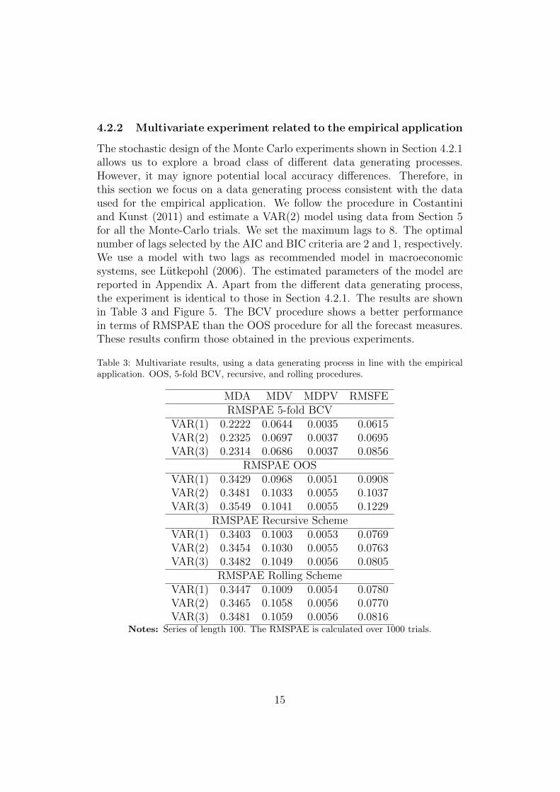
The stochastic design of the Monte Carlo experiments shown in Section 4.2.1allows us to explore a broad class of different data generating processes.However, it may ignore potential local accuracy differences. Therefore, inthis section we focus on a data generating process consistent with the dataused for the empirical application. We follow the procedure in Costantiniand Kunst (2011) and estimate a VAR(2) model using data from Section 5for all the Monte-Carlo trials. We set the maximum lags to 8. The optimalnumber of lags selected by the AIC and BIC criteria are 2 and 1, respectively.We use a model with two lags as recommended model in macroeconomicsystems, see Lutkepohl (2006). The estimated parameters of the model arereported in Appendix A. Apart from the different data generating process,the experiment is identical to those in Section 4.2.1. The results are shownin Table 3 and Figure 5. The BCV procedure shows a better performancein terms of RMSPAE than the OOS procedure for all the forecast measures.These results confirm those obtained in the previous experiments.

Table 3: Multivariate results, using a data generating process in line with the empiricalapplication. OOS, 5-fold BCV, recursive, and rolling procedures.

MDA MDV MDPV RMSFERMSPAE 5-fold BCV

VAR(1) 0.2222 0.0644 0.0035 0.0615VAR(2) 0.2325 0.0697 0.0037 0.0695VAR(3) 0.2314 0.0686 0.0037 0.0856

RMSPAE OOSVAR(1) 0.3429 0.0968 0.0051 0.0908VAR(2) 0.3481 0.1033 0.0055 0.1037VAR(3) 0.3549 0.1041 0.0055 0.1229

RMSPAE Recursive SchemeVAR(1) 0.3403 0.1003 0.0053 0.0769VAR(2) 0.3454 0.1030 0.0055 0.0763VAR(3) 0.3482 0.1049 0.0056 0.0805

RMSPAE Rolling SchemeVAR(1) 0.3447 0.1009 0.0054 0.0780VAR(2) 0.3465 0.1058 0.0056 0.0770VAR(3) 0.3481 0.1059 0.0056 0.0816

Notes: Series of length 100. The RMSPAE is calculated over 1000 trials.

15

100 200 300 400 500 600

0.0

0.3

MDA

LengthR

MS

PAE

OOSBCV

100 200 300 400 500 6000.00

0.15

MDV

Length

RM

SPA

E

100 200 300 400 500 6000.00

0

MDPV

Length

RM

SPA

E

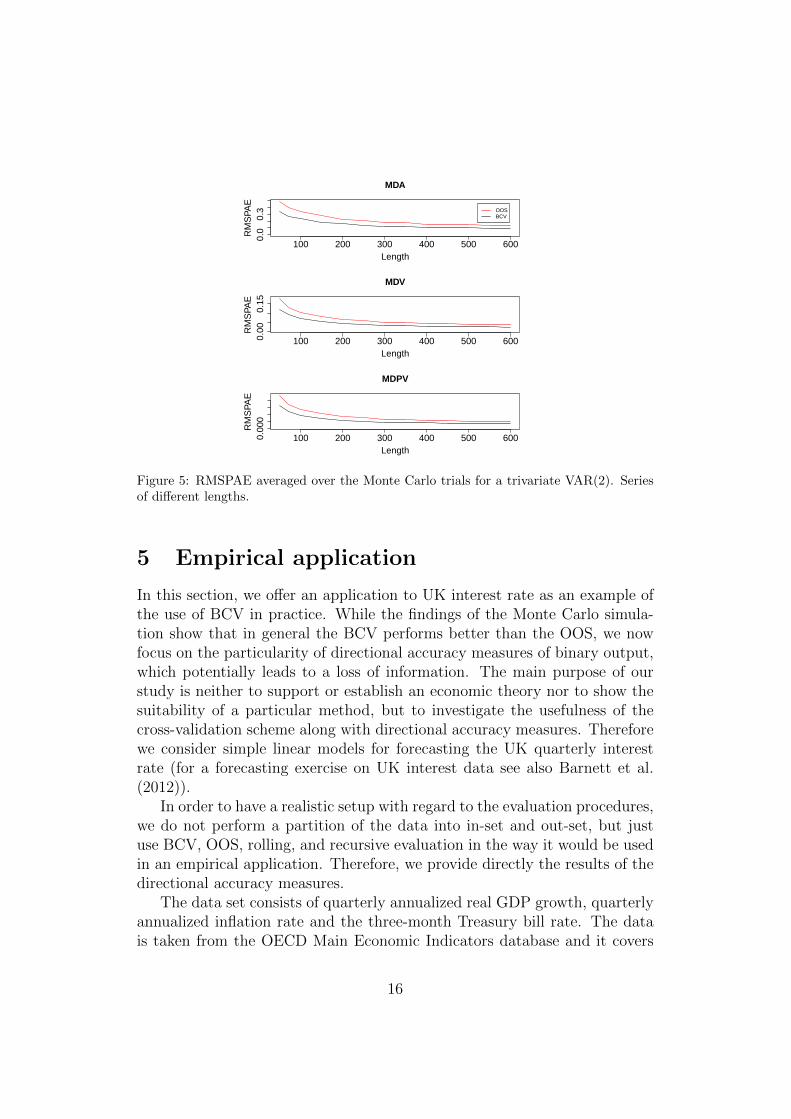
Figure 5: RMSPAE averaged over the Monte Carlo trials for a trivariate VAR(2). Seriesof different lengths.

5 Empirical application

In this section, we offer an application to UK interest rate as an example ofthe use of BCV in practice. While the findings of the Monte Carlo simula-tion show that in general the BCV performs better than the OOS, we nowfocus on the particularity of directional accuracy measures of binary output,which potentially leads to a loss of information. The main purpose of ourstudy is neither to support or establish an economic theory nor to show thesuitability of a particular method, but to investigate the usefulness of thecross-validation scheme along with directional accuracy measures. Thereforewe consider simple linear models for forecasting the UK quarterly interestrate (for a forecasting exercise on UK interest data see also Barnett et al.(2012)).

In order to have a realistic setup with regard to the evaluation procedures,we do not perform a partition of the data into in-set and out-set, but justuse BCV, OOS, rolling, and recursive evaluation in the way it would be usedin an empirical application. Therefore, we provide directly the results of thedirectional accuracy measures.

The data set consists of quarterly annualized real GDP growth, quarterlyannualized inflation rate and the three-month Treasury bill rate. The datais taken from the OECD Main Economic Indicators database and it covers

16

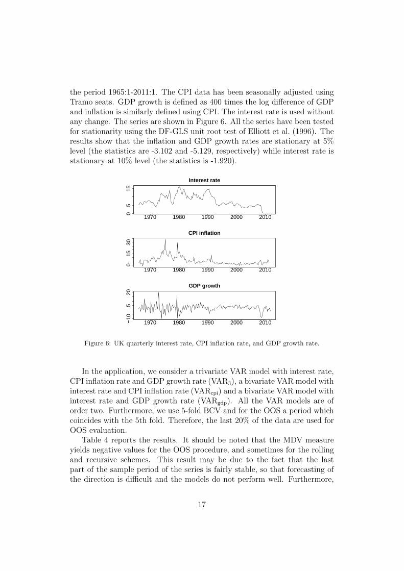
the period 1965:1-2011:1. The CPI data has been seasonally adjusted usingTramo seats. GDP growth is defined as 400 times the log difference of GDPand inflation is similarly defined using CPI. The interest rate is used withoutany change. The series are shown in Figure 6. All the series have been testedfor stationarity using the DF-GLS unit root test of Elliott et al. (1996). Theresults show that the inflation and GDP growth rates are stationary at 5%level (the statistics are -3.102 and -5.129, respectively) while interest rate isstationary at 10% level (the statistics is -1.920).

1970 1980 1990 2000 2010

05

15

Interest rate

1970 1980 1990 2000 2010

015

30

CPI inflation

1970 1980 1990 2000 2010−10

520

GDP growth

Figure 6: UK quarterly interest rate, CPI inflation rate, and GDP growth rate.

In the application, we consider a trivariate VAR model with interest rate,CPI inflation rate and GDP growth rate (VAR3), a bivariate VAR model withinterest rate and CPI inflation rate (VARcpi) and a bivariate VAR model withinterest rate and GDP growth rate (VARgdp). All the VAR models are oforder two. Furthermore, we use 5-fold BCV and for the OOS a period whichcoincides with the 5th fold. Therefore, the last 20% of the data are used forOOS evaluation.

Table 4 reports the results. It should be noted that the MDV measureyields negative values for the OOS procedure, and sometimes for the rollingand recursive schemes. This result may be due to the fact that the lastpart of the sample period of the series is fairly stable, so that forecasting ofthe direction is difficult and the models do not perform well. Furthermore,

17

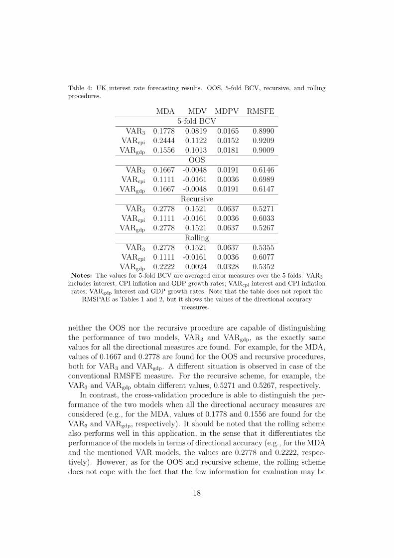
Table 4: UK interest rate forecasting results. OOS, 5-fold BCV, recursive, and rollingprocedures.

MDA MDV MDPV RMSFE5-fold BCV

VAR3 0.1778 0.0819 0.0165 0.8990VARcpi 0.2444 0.1122 0.0152 0.9209VARgdp 0.1556 0.1013 0.0181 0.9009

OOSVAR3 0.1667 -0.0048 0.0191 0.6146

VARcpi 0.1111 -0.0161 0.0036 0.6989VARgdp 0.1667 -0.0048 0.0191 0.6147

RecursiveVAR3 0.2778 0.1521 0.0637 0.5271

VARcpi 0.1111 -0.0161 0.0036 0.6033VARgdp 0.2778 0.1521 0.0637 0.5267

RollingVAR3 0.2778 0.1521 0.0637 0.5355

VARcpi 0.1111 -0.0161 0.0036 0.6077VARgdp 0.2222 0.0024 0.0328 0.5352

Notes: The values for 5-fold BCV are averaged error measures over the 5 folds. VAR3

includes interest, CPI inflation and GDP growth rates; VARcpi interest and CPI inflationrates; VARgdp interest and GDP growth rates. Note that the table does not report the

RMSPAE as Tables 1 and 2, but it shows the values of the directional accuracymeasures.

neither the OOS nor the recursive procedure are capable of distinguishingthe performance of two models, VAR3 and VARgdp, as the exactly samevalues for all the directional measures are found. For example, for the MDA,values of 0.1667 and 0.2778 are found for the OOS and recursive procedures,both for VAR3 and VARgdp. A different situation is observed in case of theconventional RMSFE measure. For the recursive scheme, for example, theVAR3 and VARgdp obtain different values, 0.5271 and 0.5267, respectively.

In contrast, the cross-validation procedure is able to distinguish the per-formance of the two models when all the directional accuracy measures areconsidered (e.g., for the MDA, values of 0.1778 and 0.1556 are found for theVAR3 and VARgdp, respectively). It should be noted that the rolling schemealso performs well in this application, in the sense that it differentiates theperformance of the models in terms of directional accuracy (e.g., for the MDAand the mentioned VAR models, the values are 0.2778 and 0.2222, respec-tively). However, as for the OOS and recursive scheme, the rolling schemedoes not cope with the fact that the few information for evaluation may be

18

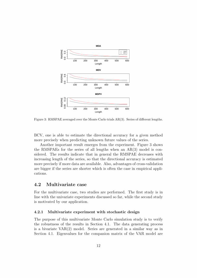
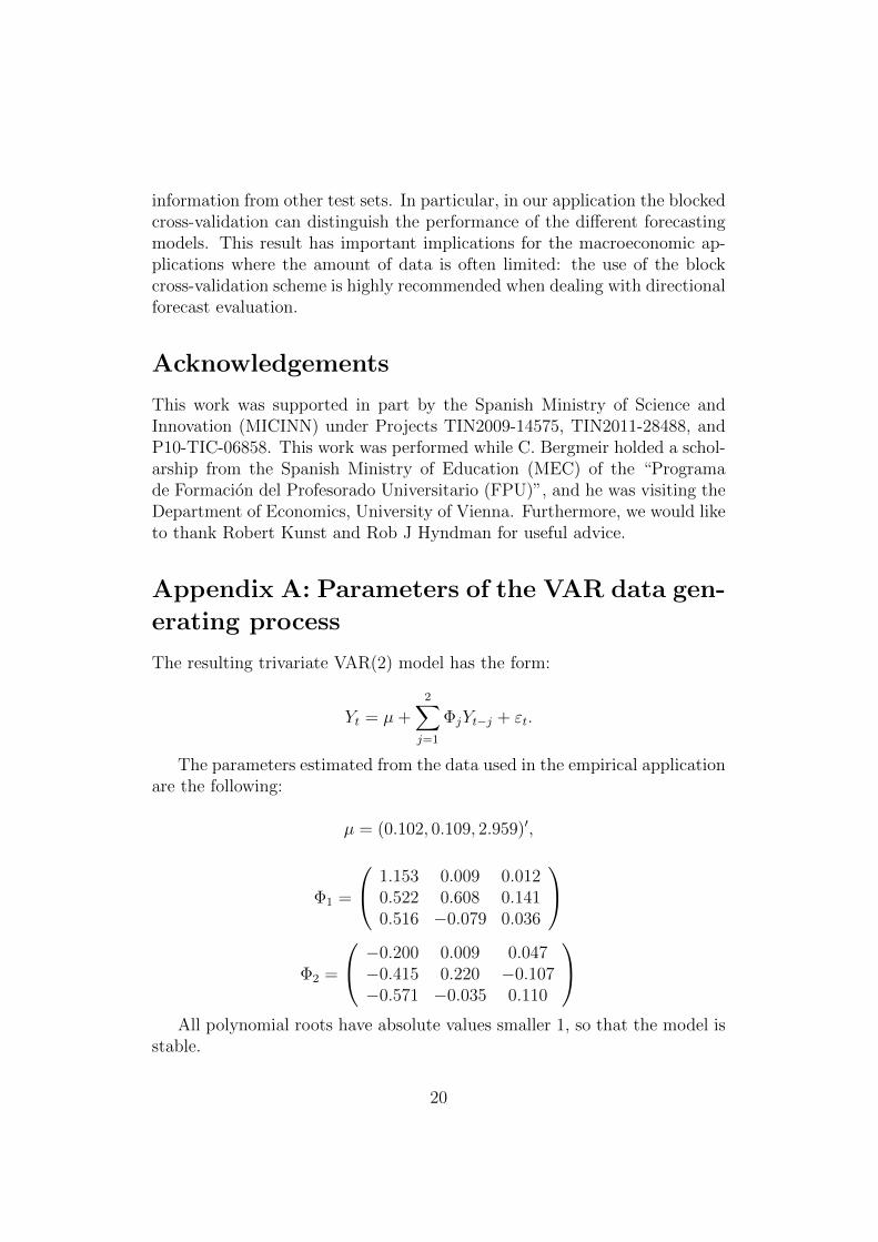
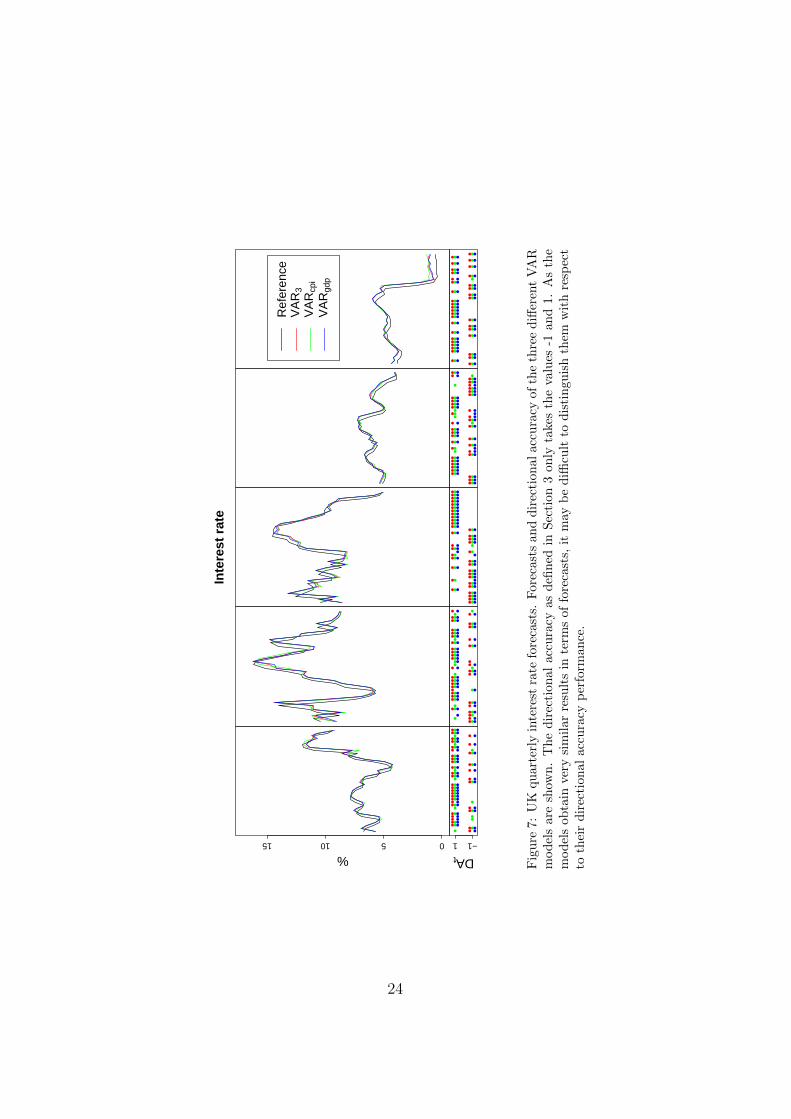
not enough to distinguish the performance of the models.Furthermore, the results are examined in more detail in Figure 7. We

focus on the BCV and OOS procedures (similar results to OOS are foundfor rolling and recursive schemes). It should be noticed that in the last foldof BCV, which is also used for OOS, all models yield identical results interms of the directional accuracy, with the exception of the VARcpi whichyields an incorrect directional forecast in one case (the other two modelsare able to predict the direction correctly). Using OOS, only the informa-tion from the 5th fold is used, and the VAR3 and VARgdp models yield thesame results on this fold. In contrast, BCV uses forecasts of all folds, sothat it helps distinguish the forecasting performance of the models in termsof directional forecast accuracy. These results have important implicationsfor macroeconomic applications where the amount of data available can belimited: the use of the blocked cross-validation is highly recommended fordirectional forecasts.

6 Conclusions

This paper investigates the usefulness of a predictor evaluation frameworkwhich combines a k-fold blocked cross-validation scheme with directionalaccuracy measures. The advantage of using a blocked cross-validation schemeover other procedures such as the standard out-of-sample procedure is thatthe blocked cross-validation allows one to obtain a more precise error estimateof the generalization error from the data as it uses all the available data bothfor training and testing.

In this paper we evaluate whether, and to what extent, the k-fold blockedcross-validation procedure may provide more precise results than the stan-dard out-of-sample procedure even when dealing with directional forecastaccuracy. To this end, a Monte Carlo analysis is performed using simpleunivariate and multivariate linear models. The results show that the blockedcross-validation is able to estimate the directional accuracy more preciselythan the out-of-sample procedure when predicting unknown future values ofthe series. These results are obtained in both the univariate and multivariatedesign.

An empirical application is also carried out on forecasting UK interestrate data using three different simple VAR(2) models. The limited amountof available data, together with the use of directional accuracy measures,leads to identical realized average loss/success on some occasions when usingthe standard out-of-sample procedure. The blocked cross-validation is lesslikely to yield identical estimates for a given sample size, as it uses additional

19

information from other test sets. In particular, in our application the blockedcross-validation can distinguish the performance of the different forecastingmodels. This result has important implications for the macroeconomic ap-plications where the amount of data is often limited: the use of the blockcross-validation scheme is highly recommended when dealing with directionalforecast evaluation.

Acknowledgements

This work was supported in part by the Spanish Ministry of Science andInnovation (MICINN) under Projects TIN2009-14575, TIN2011-28488, andP10-TIC-06858. This work was performed while C. Bergmeir holded a schol-arship from the Spanish Ministry of Education (MEC) of the “Programade Formacion del Profesorado Universitario (FPU)”, and he was visiting theDepartment of Economics, University of Vienna. Furthermore, we would liketo thank Robert Kunst and Rob J Hyndman for useful advice.

Appendix A: Parameters of the VAR data gen-

erating process

The resulting trivariate VAR(2) model has the form:

Yt = µ+2∑j=1

ΦjYt−j + εt.

The parameters estimated from the data used in the empirical applicationare the following:

µ = (0.102, 0.109, 2.959)′,

Φ1 =

1.153 0.009 0.0120.522 0.608 0.1410.516 −0.079 0.036

Φ2 =

−0.200 0.009 0.047−0.415 0.220 −0.107−0.571 −0.035 0.110

All polynomial roots have absolute values smaller 1, so that the model is

stable.

20

The variance-covariance matrix has the following form:

Σ =

0.882 0.530 0.3190.530 8.100 −2.1340.319 −2.134 14.145

References

C. Altavilla and P. De Grauwe. Forecasting and combining competing modelsof exchange rate determination. Applied Economics, 42:3455–3480, 2010.

S. Arlot and A. Celisse. A survey of cross-validation procedures for modelselection. Statistics Surveys, 4:40–79, 2010.

A. Barnett, H. Mumtaz, and K. Theodoridis. Forecasting UK GDP growth,inflation and interest rates under structural change: a comparison of mod-els with time-varying parameters. Working Paper 450, Bank of England,2012.

C. Bergmeir and J.M. Benıtez. Forecaster performance evaluation with cross-validation and variants. In International Conference on Intelligent SystemsDesign and Applications, ISDA, pages 849–854, 2011.

C. Bergmeir and J.M. Benıtez. On the use of cross-validation for time seriespredictor evaluation. Information Sciences, 191:192–213, 2012.

O. Blaskowitz and H. Herwartz. Adaptive forecasting of the EURIBOR swapterm structure. Journal of Forecasting, 28(7):575–594, 2009.

O. Blaskowitz and H. Herwartz. On economic evaluation of directional fore-casts. International Journal of Forecasting, 27(4):1058–1065, 2011.

O. Blaskowitz and H. Herwartz. Testing directional forecast value in thepresence of serial correlation. International Journal of Forecasting, 30(1):30–42, 2014.

A. Blum, A. Kalai, and J. Langford. Beating the hold-out: Bounds for k-fold and progressive cross-validation. In Proceedings of the InternationalConference on Computational Learning Theory, pages 203–208, 1999.

S. Borra and A. Di Ciaccio. Measuring the prediction error. A comparisonof cross-validation, bootstrap and covariance penalty methods. Computa-tional Statistics & Data Analysis, 54(12):2976–2989, 2010.

21

G.N. Boshnakov and B.M. Iqelan. Generation of time series models withgiven spectral properties. Journal of Time Series Analysis, 30(3):349–368,2009.

J. Chung and Y. Hong. Model-free evaluation of directional predictability inforeign exchange markets. Journal of Applied Econometrics, 22:855–889,2007.

M. Costantini and R. Kunst. Combining forecasts based on multiple encom-passing tests in a macroeconomic core system. Journal of Forecasting, 30:579–596, 2011.

M. Costantini and C. Pappalardo. A hierarchical procedure for the combi-nation of forecasts. International Journal of Forecasting, 26(4):725–743,2010.

G. Elliott, T.J. Rothenberg, and J.H. Stock. Efficient tests for an autore-gressive unit root. Econometrica, 64:813–836, 1996.

T. Hastie, R. Tibshirani, and J. Friedman. Elements of Statistical Learning.Springer, 2009. ISBN 9780387848846.

R.J. Hyndman and A.B. Koehler. Another look at measures of forecastaccuracy. International Journal of Forecasting, 22(4):679–688, 2006.

J.A. Khan, S. Van Aelst, and R.H. Zamar. Fast robust estimation of predic-tion error based on resampling. Computational Statistics & Data Analysis,54(12):3121–3130, 2010.

T.-H. Kim, P. Mizen, and T. Chevapatrakul. Forecasting changes in UKinterest rates. Journal of Forecasting, 27(1):53–74, 2008.

Q. Kong. Predictable movements in yen/dm exchange rates. IMF workingpaper 143, 2000.

R. Kunst. Cross validation of prediction models for seasonal time seriesby parametric bootstrapping. Austrian Journal of Statistics, 37:271–284,2008.

H. Lutkepohl. New Introduction to Multiple Time Series Analysis. Springer,2006. ISBN 9783540262398.

A.D.R. McQuarrie and C.-L. Tsai. Regression and time series model selec-tion. World Scientific Publishing, 1998.

22

C. Milas and R. Naraidoo. Financial conditions and nonlinearities in theEuropean Central Bank (ECB) reaction function: In-sample and out-of-sample assessment. Computational Statistics & Data Analysis, 56(1):173–189, 2012.

R Development Core Team. R: A Language and Environment for StatisticalComputing. R Foundation for Statistical Computing, Vienna, Austria,2009. URL http://www.R-project.org. ISBN 3-900051-07-0.

J. Racine. Consistent cross-validatory model-selection for dependent data:hv-block cross-validation. Journal of Econometrics, 99(1):39–61, 2000.

N. Solferino and R. Waldmann. Predicting the signs of forecast errors. Jour-nal of Forecasting, 29(5):476–485, 2010.

S. Sosvilla-Rivero and E. Garcıa. Forecasting the dollar/euro exchange rate:Are international parities useful? Journal of Forecasting, 24:369–377, 2005.

23

051015

Inde

x

%

●●

●●

●●

●

●●

●●

●●

●●

●●

●●

●●

●

●

●

●●

●

●

●●

●

●●

●

●●

DAt

●

●

●●

●●

●

●

●●

●

●●

●●

●●

●

●●

●●

●

●

●●

●

●●

●●

●●

●●

●

●●

●●

●●

●

●●

●●

●●

●●

●●

●●

●●

●

●

●

●●

●

●

●●

●

●●

●

●●

−11

●●

●●

●

●●

●●

●●

●●

●●

●●

●

●●

●●

●●

●

●

●

●●

●

●●

●●

●

●

myMDA("VAR3", 2, a = 1.3)

●

●

●●

●●

●

●●

●

●

●●

●●

●

●●

●●

●●

●●

●

●●

●●

●

●●

●●

●

●●

●

●

●

●

●●

●●

●

●

●●

●●

●●

●

●

●●

●●

●

●

●

●

●●

●

●●

●●

●

●

Inte

rest

rat

e

●●

●●

●

●●

●

●●

●

●

●●

●●

●

●●

●●

●

●

●

●●

●●

●●

●●

●●

●●

myMDA("VAR3", 3, a = 1.3)●

●●

●

●

●●

●

●●

●

●

●●

●●

●

●

●●

●●

●

●

●●

●●

●●

●●

●●

●●

●●

●●

●

●●

●●

●●

●

●●

●

●

●●

●

●●

●

●

●

●●

●●

●●

●●

●●

●●

●●

●

●●

●●

●●

●●

●

●

●

●

●●

●

●

●

●●

●

●

●●

●●

●●

●●

●●

●●

myMDA("VAR3", 4, a = 1.3)

●●

●

●●

●●

●●

●

●●

●

●

●

●●

●

●●

●

●●

●●

●●

●

●●

●

●

●●

●

●

●●

●

●●

●●

●●

●●

●●

●

●

●●

●

●

●

●●

●●

●●

●●

●●

●●

●●

●●

Ref

eren

ceV

AR

3V

AR

cpi

VA

Rgd

p

●

●

●●

●●

●●

●

●

●

●●

●

●

●●

●●

●●

●●

●

●●

●●

●

●●

●

●

●

●

●

myMDA("VAR3", 5, a = 1.3)

●

●

●●

●●

●●

●

●

●

●●

●

●

●●

●●

●●

●●

●

●●

●

●●

●●

●

●

●

●

●●

●

●●

●●

●●

●

●

●

●●

●

●

●●

●●

●●

●●

●

●●

●●

●

●●

●

●

●

●

●

Fig

ure

7:U

Kqu

arte

rly

inte

rest

rate

fore

cast

s.F

ore

cast

san

dd

irec

tion

alacc

ura

cyof

the

thre

ed

iffer

ent

VA

Rm

od

els

are

show

n.

The

dir

ecti

onal

accu

racy

asd

efin

edin

Sec

tion

3only

take

sth

eva

lues

-1an

d1.

As

the

mod

els

obta

inve

rysi

mil

arre

sult

sin

term

sof

fore

cast

s,it

may

be

diffi

cult

tod

isti

nguis

hth

emw

ith

resp

ect

toth

eir

dir

ecti

onal

accu

racy

per

form

ance

.

24