Embed Size (px)
Citation preview
NVADC TEC11N:ICAL REiPoirr 58-17 ?*'42O2
ON THE USE OF QUATERNIONS IN SIMULATIONOF RIGID-BODY MOTION
Alfred C. Robinson
Aeronautical Research Laboratory
DECEMBER 1958
/
Reproduced FromBest Available Copy
WRIGHT AIR I)EVELOPMENT CENTER
(
REPRODUCED BYNATIONAL TECHNICAL
INFORMATION SERVICEU.S. DEPARTMENT OF COMMERCE
SPRINGFIELD, VA. 22161
NO rICES
When Goverrnment drawings, specifications, or other data are used for any purpose other
than in conn.rction with a definitely relazed Government procurement operation. the United States
Gove-rnment thereby incurs no responsibility nor any obligation whatsoever: and the fact that
the Governmnent may have formulated- furnished, or in any way supplied the said drawings,
sps-cifications. or e.ther data. is not to be regarded by implication or otherwise as in any manner
lic(,ning the holder or any other person or corporation, or conveying any rights or permissionto manufacture. use. or sell any patented invention that may in any way be related thereto.
Qualit.-d requesters may obtain copies of this report from the Armed qervices TechnicalInf.,mator. AgenCy. oASTIAi. Arlingto-n Hall Station. Arhngton 12. Virginia.
Thic report ba3: been released to the Office of Technical Srrvices. U. S. Department of Corn-merce. Wa.nington 25. D. C.. for sale to the general public.
Copi'-'s -f WADC Technical Repor.s and Technical Notes should not be returned to the WrightAir Development Center unless return is required by security considerations, contractual ob!iga-tiors, or notice on a specific document.
I

NOTICE
THIS DOCUMENT HAS BEEN REPRODUCED
FROM THE BEST COPY FURNISHED US BY
THE SPONSORING AGENCY. ALTHOUGH IT
IS RECOGNIZED THAT CERTAIN PORTIONSAfE ILLEC-IBLE, IT IS BEING RELEASED
iN THE INTEREST OF MAKING AVAILABLE
AS MUCH INFORMATION AS POSSIBLE.
I
A,
I X~~VADC 'IECIINICA L RETPORF 58-17
ON 1HE USE OF QUATERNIONS iN SIMULATIONOF RIGID-BODY MOTION
A?/1ned C. Robinson
A eron autical Researchi La boratory
I ~DECEMABER i9;-)8
J Project No. 7060
NVIUGH-T All? DEVEILOM01IMENT CENTERAllR. BSFARCI- A1ND1 DEiVEL"OPMAENT 'COMM%,AND
UNITED STATES AIR FORCE
WI{IGHiT-PATT'I'ISON AIR FORCE BfASE--, 011IO
wo- March 1960- 24-680
FOREWORD
The work CO-IvL red by this repolt was done the System Dynamics Branch,.Avronautical Research Laboratory, under Pr-.,n-z-t 7060, "Flight DynamicsResearch and Analysis Facility". Mr. Paul. W• Nosker is Project Engineer."This study Is part of a continuing program to t-:ermi.ne optimum methods ofsimulation 2tnd analysis of the dynamics of ai-r- weapon systems. The generalsubject of quaternions as applied to coordinara conversions has been underinvestigation for approximately two years, thcz•uzh the bulk of the work reportedhcre was accomplished during the lastsix mrnmins of 1957.
The author wishes to express his appreciarzion to Mr. Robert T. Harnett andothers of the Analog Computation Branch of Lit,- -Aeronautical Research Laboratoryfor assistance in the analog simulation portinre n~f the study.
W-ADCL TR A8-17
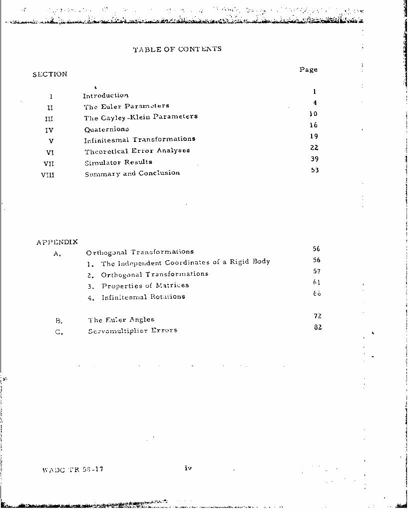
TABLE OF CONTENTS
SECTION Page
I Introduction 1
II The Euler Parameters 4
III The Cayley -Klein Parameters 10
IV Quaterniono 16
V Infinitesrnal Transformations 19
VI Theoretical Error Analyses zU
VII Simulator Results 39
VIII Sumiriary and Conclusion 53
APPENDIX
A. O rthogonal Transqforrnations 56
1. The Independent Coordinates of a Rigid Body 56
a. Orthogonal Transformations 57
3. Properties of Matrices 61
4. Infinitesmal Rotations 6
B. The Fuier Angles 72
\'WA DC.1 "'R 53 -17 iv
A lAST RA CT
The theory of the four-parameter mnethod is dev,-loped with specificapplication to coordinate conversion in aircraft simulatioris. This method
is compared with the direction cosine method both io a theoretical erroranalysis and in an example simulation on an analog computer. It is shown
that the quaternion method is no more sensitive to multiplier errors than
is the direction cosine method, and it requires nearly 30 per cent lesscomputing equipment, In addition, the multiplier bandpass re;aoirernent
in the four-parameter method is onlyl half as severe as for direction cosines.
By every important criterion, the quaternion method is no worse than, and
in most cases, better than the direction cosine method.
N8W ADG TR 58.47 iin
SECTION I
INTRODUCTION
The problem of motion of a rigid body and the associated one of coordinate
copversion are very old ones in the field of classical dynamics. Significant
results, dating from the time of Euler (1776) thrcugh the introduction and
appltcation of matrix methods by Cayley and Klein and others in the last half
of the nineteenth century, brought the matter to such a satisfactory state that
no significantly new methods or approaches have been found necessary. The
developmnent of modern computing machinery makes necessary a re-ezarnination
of the -iaricus methods from the standpoint of their utiiity in computational
devices, it is not necessarily true that methods which have proven their con-
venience in the largely ar,.lytical manipulations of classical mechanics should
prove to be best adapted .or nuraiezical or a ialog computation. Quaternions fell
into disuse among physicists about the turn of the present centur': because matrix
and vec'tor methods had proved more useful in the types of investigations then
b.-;ing conducted. The purpore of the present paper is to show that the quaternion
anproa:.h to coordinate transformation does sffer real advantages in ýhe anaiog
simulation of rigid body motion. In recent times Deschamps and Sudduth* have
sugge.;ted an applialli 'oCL , Uital co..i.pdLtation, and Eackus** has proposed them
for analog sim'ulation, but in general quaternions are little known among t.hose
engaged in si.mulation of aircraft motions,
The coordinate conversion problemn in aircraft and missile simulation is
different at least in emphasis from that of classical dynamnics., It might be well
to state the problem which is of interest and to which the methods explained later
will be applied. A missile or aircraft znay be considered as a moving coordinate
system, Various vectors must be transformed into this coordinate system or out
*Deschazxips, G. A. and IV. B. Sudduth, Federal Telvcommunications Laboratories,
Nutley, New Jersey. Case ?6-10707, November 1955. . -
44 .•lg*ijackus, Ce-orge, Rigid Body Equations - Euler Parameteris, Technical Note 6,
Advisory Board on Simulation, University of Chicago, November 1951.
Manus,.ript released by author 15 January 1958 for publication as a WADC TechnicalReport.
WADC TP. 58-17 1
.•o , - - -. - .
a. i..t -. s. "A 4 ': - .- *. ~< j.- . .. • - .- - " " - - .. . . -. . .
of it into some inertial system. Integrating the equations of motion of the air-
frame can be made to yield the three components of the coordinate system's
angular velocity vector. From the X, Y and Z components (P. Q, R) of this
vector in the moving system, it is desired to keep track of the orirutation of
the coordinate system in sach a way that vectors may be transformed in either
direction. This means an integration of angular rate to dete-arrne angular
position.
Fundamental to this procedure is a consideration of how the orientation of
the coordinate system is to be specified. During the history of the subject,
varixus methods of doing this have been put forward. AlL the most useful onles
fail into three categories: Euler angles, quaternions, and direction cosines.
Of these, the first and last are probably the most familiar to modern readers.
In the Euler angle method, the orientation is expressed as the result of three
rotations about each of ti-ree axes, the rotations being made in a specific
sequence. The physical interpretation of a ouateainion is a rotation through sorne
arigle about some specific fixed axis. The nine direction cosines are simply the
cosiai.cs of the angles between each of the axes in the moving system with each
of the axes of the fixed system. Principal attention here will be given to the
quaternion, or four-parameter system. It was first introduced by Euler in 1776,
ý a- rvCsult of spherical trigonometry consideaations. The elegant quaternion
form•ulation was invented by Ilamilton in 1843 as a new kind of algebraic ftnmal-
isan. A natrix formulation was devised by Klein for use in gyroscopic pioblems
an-d, in this formulation, is usually known as the Cavicy-Klein parameters. Each
c? the2se three different approaches to the foocr-param-ter system has its own
advantages. It has been decided to present at least an outline of all three here.
There are two reasons ior this: first, there are somne propositionbs wh;ch are more
easily shown by ono development; secnnd, it seems probable that when the reader
is offercd a %hoice oi method, he will reach zan understanding sooner if he cýis
select .he method most nearly consonant with his own backgxound.
It will become apparent that this subject presents something of an expositional
Ci problem. In order to reach the desired ends, it has been deciemd to assume that
the reader has a knowledge of matrix methods, especially as applied t,.o coordinate
conversion in three-dinicusional space. As a compromise, a brief introduction
to thu subject is given in Appendix A, though a more satisfactory trea!.ment ia
given by Goldstein*. In this i eport the term "quatern.on" has been us;ed tz
[I
: *..lteii, lHerbert, Classical Mechanics Addison-Wesley Press, C:air.bridge,
.Mass., 1950.
WAC TIR 5S-I7 -17.
represcint the fo-r-parameter method in general. In other cases, it is necessary
to use the word to distinguish Hansyiltoji's development from the others. It is hoped
that conftusion may be kept to a min~nuin.
There arc ma3ny different tcchn.ques used in present-day aircraft simulations to
solve the coordinate conversion prob.em. I he technique is usually adapted to the
spfecial requirements of the problem at hand. Ii most of the rotation takes place
Lbout one axis, or if only the gravity vrector is to be handled, or i-f the airframe's
rotation is otherwise restricted, valuable sirmplifications may be effected in the
analog equipment required to represent the conversion. It is not the present
purpose, howvever, to investigate all these possibilities. Consideration will be
given only to the. moss general and unrestricted case: that of several complete
revolutions about any cr all axes. This immediately excludes the Euler angles
because of the singular point. The advantages of Euler angles are such, and their
popularity is so pervasive, however. as to warrant keeping them in mind. Accordingly,
Appendix B gives a brief outline of the Euler Angle system most commonly used in
aircraft work, and at appropriate points, comparisons will be made of them with
quaternions and direction cosines. In making such comparisons, that form of Euler
angle instrumentation whose capabilities most nearly equal those of the quaternion
scheme will be asýurned. This form has been discussed at some length by liowe*
and his figures and results wi". be used for comparison, in Howe. s method, the
extent ant. direction of rotation is unrescricted except for the inevitable singular
orientation, and he shows that even this leads to less practical difficulties than one
inight expect.
It is valuable to keep the Euile2r angles in mind, but the quaternion method must
really st.r~d or fall on Lts cromparlson with direction cosines. It has in common
with direction cosines the cal ability of handling completely unrestricted rotations.
Accordingly, considerable attcz.tiin h-las been devoted to the direction cosine method
in L-is report. Both a theoretical error amalysis and a simulation program were done
for the cosines in order tc provide the most complete possible basis of compnriso1n,
They have been done before, bLt it is difficult to compare results obtained by
dilferent investigators on dIfft ent computing equipment. An attempt waE made here
to keep the coiditions as nearly comparable as possible. Of all the material con-
tained herein, no or'ginality is claimned exrept for rhe quaternion error analysis
and simulation. Even here, no ne'.v techniques were used, with the possibleexcept.ion of the method of handling multiplier errors. It wzs felt necessary,
however, to include the remaining material in order to introduce and place in
context this probably unfamiliar subject.
*JThwe, R. M. and E. G. Gilbecn, A New Resolving Method for Analog Computers,WADC Technical Note 55-467, YJ-uary 1956.
WADC TR 58-17 3
SECTION 11
"TH1rE EULER PARAMETERS
The earliest formulation of the four-parameter system was given by Euler
1 776, thuugh the oldest treatment generally available today is probably that
of Whittaker*. It is an essentially geometrical dcveloprrment, but will not be
presented cas such here. The principal results may be denmonstrated with much1 ess labor by use of matrices.
Central to the development of these parameters, and indeed to the four-
pararietet methods in general, is the proposition known as Euler's theorem,
which may be stated as follovw s: any real rotation may be expressed as a
rotation through some angle, about sonic fixed axis. In other words, regard-
less of what the rotation history of a body is, once it reaches some orientation,
that orientation n.,y be specified in terms of a rotation through some angle (which
can be determined) Libout some fixed axis.
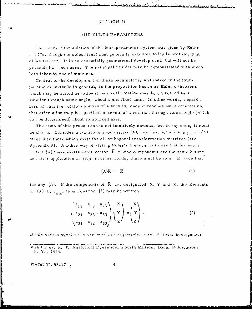
The truth of this proposition is net intuitively obvious, but in any case, it must
be shown. Consider a transformation matrix (A). No restrictions are u.ut on (A)
other than those which exist for all orthogonal transformation matrices (see
Appendix A). Another way of stating Euler's theorem is to say that for every
matrix (A) there exists some vector R whose components are the sanme before
ant,'ifte•r application of (A); in other words, there must be rome _R sach th-at"
(A)ik = R.(1)
for any (A). If the components of P. are designated X, Y and Z, the oleyoents
of (A) by a-n, then Equation (1) nay be written
•":a 1 & Z a?., Y uZ)a1 2z a 3
Sa31 3Z 3
If this matrix equation is expanded in components, a set of linear homogenous
r *Whit.,,i: r, 15. 1. Analytical Dynamics, Fourth Edition, Dover Publications3
N. Y., 1)44.
\VADCG TR 58-17 4
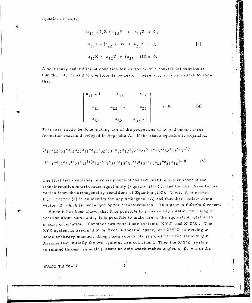
'.quatiorts results:
(a 1 1 - I)X + altY + a.! 3 Z 0,
a 2 1 X + (a - 1)Y + a 4 3 Z = o, (3)
a 3 1 X f a3 2 Y + (a 3 3 - 1)Z = 0.
A necessary and sufficient condition for existence of a ron-trivial solution is
that the determinant of coefficients be zero. Tiereforc, it is necessary to show
that
a 1 1 -a1 1 2 a 1 3
a 2 1 aaz - 1 a 2 3 - . (4)
a 3 1 a 3 2 a331
This may easily be done making use of the properties of arn orthigonal trana-
io:.nation matrix developed in Appendix A. If the above equation is expanded,
(a1a'Ra 3 3+al2a2 3 '31 2132 1 3 -a 3 1 a 1 3 a, 2 -a21 a12a33 a3a2
+(a 1 1 -a 2za 3 34+a 2 3 a3 I)+(a2 -aa31 3 +'13'3 1)('33-a '2Z21 li 2, )= 0 (5)
'rh,ý first term vanishes in consequence of the fact that the deterrfn.r4nt of the
transformation matrix must equal unity (Equation (1356) ), arid tic last Lhrue terms
vanish from the orthogonality conditior.s of Equationi (16Z). Thus, it is oroved
that Equation (%4) i-s an identity For any orthogonal (A) and that ther. existr some-
vector R which is unchanged by the transformation. This proves Euler's theorem, r(dSince it has been shown that it is possible to express any rotation as a single
rotation albout some axis, it is possible to make use of the equivalent rotation to
specify orientation. Consider two coordinate systems X Y Z and X' Y' Th.
XYZ system is assumed to be fixed in inertial space, and X'KY'Z' is moving in,
some arbitrary manner, though both coordinate systems have the same oligin.
Assume that initially the two systems are coincident. Thern the X'Y'Z' system
is zotated through an angle F' about an axis which makes angles n, Y, y with the;
WADC TR 58-17
Ar
aSS•
A
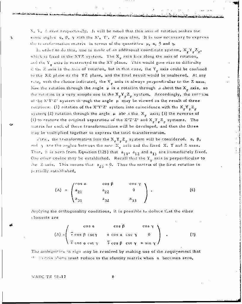
\,•I 'z /. s. respectivc!x . It l ill be noted that this itxis of rotation nLialcs thes• ic .oghcs ,o, [3, '•" .vith the \', Y', Z' axes \l5so. It is 1low necessary to expr,_s:
t I. i .ns-.fori'xtion Matrix in terms of the quantities p, a, '3 and -y.
I:u, r.,r to do this *use is made of in addititonal coordinate syste°rn, X r Z" • ~r r r
%01.h,-i.; l7ix ed in the XYZ sy.stem. he Xr axis lies along the axis of rotation,
1C the Y raxis is restricted to the XY plaine. This would give rise to difficultyr
i' thte 7 axis is the axis of rotation, but in that case, the Y r-axis could be confinedr
to the XZ pl.-me or the YZ plane, and the final result would be unaltered. At any
r-.:e, with the choice indicated, the Yr axis is always pec-pendicular to the Z axib,.
Now the rotation through the angle j± is a rotation through 4. about the Xr axis, so
the rt ,,iton is a very simple one in the X Y Z system. Accordingly, the rotrtinr r r
o 'lhe .' Y'Z' system th-ough the angle p. may be viewed as the result of threerotarions: (1) rotation of the X'Y'Z' system into coincidence with the X rY rZ
rr r
systev; (2) rotation through the angle ý± abc' . the X axis; (3) the reverse oft_1 r
(1) to restore the original separation of the X'Y'Z' and X Y 7Z systems. The
n iatrix fur cacd. of these transformations will be developed, and then the three
-izay be mnultiplied together to express the total tiansformation.
-irsL, the transformation into the X Yr Zr system will be considered, a, ,
,1:,d y are the ang!les hetw.een thec ne.' X a"is anrd the fixed X, Y and Z axes.Ti'us, it is seen: from Equation (125) that all a and a13 are immediately fixed.
One other cosine may be established. Recall that ihe Y axis is perpendicular to
• .Z axis. PIhis mneans that a 2 3 = 0. Thus the matrix of the first rotation is
Cos a Cos Cos '(A) = (6) a 2 0 .
S31a 3 a 3a /
Applying the orthogonality conditions, it is possible to, deduce t:.at the other
leirients are
cosC Cos3 cos ,Y
(A) 7 Cos fi Cscy Cos a CsC 0 (7)
T c0!30. •cot ' Tcos P cot y :c sin 0
The amhbigiit.,"s 'n sign mnay be resolved by making use of the requirement that
l f.-itrix zovc must reduce to the identity matrix when a becomes zero.
A1'ADO T . 3-17 6
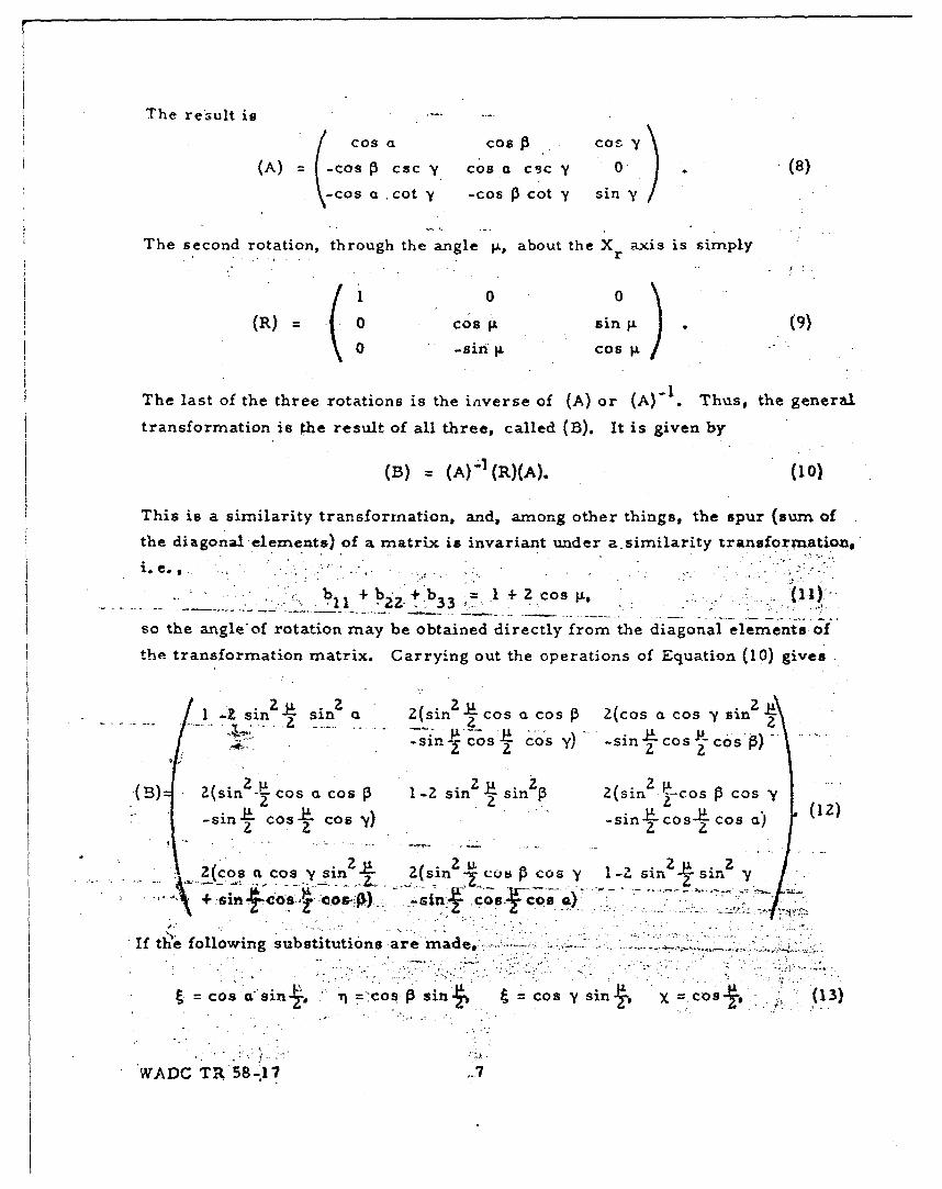
The result iscos a COB . cos
(A) -Cos P csc Y cos a csc ,Y 0, (8)
-cos a .cot Y -cos P cot sin y
The second rotation, through the angle p, about the X rax-is is simply<'0 O0(R) 0 cos I sinp . (9)
0 -sin IL Cos Ft "
The last of the three rotations is the inverse of (A) or (A) . Thus, the general
transformation is phe result of all three, called (B). It is given by
(B) = (A)-'(R)(A). (10)
This is a similarity transformation, and, among other things, the spur (sum of
the diagonal elements) of a matrix is invariant under a.similarity transforrnation,
1. .,C.. ..
., : b• + bz + b• 1= +l 2 Cos i.. . ;• ib1 1 +bz 3 3 + os,()
so the angle'of rotation may be obtained directly from the diagonal elements of
the transformation matrix. Carrying out the operations of Equation (10) gives
1sin - osin 2 a 2 insinnCos CosZ Z(cos a-cos y sin
"s -Ci-o-OSn• -S Cos Y) -sin -cos- c
• (osn cos a cos 1-2 sin sin- 2 (si- Con Cs Y
.... -siny cos-Ieos) -sinEccos L cos a)
._(cos ct os Ysin2 ~~ 2(sn c cos y I-Z ~si Siny
+.Si 'Cs -CSP -I Cos- Cos a
If tlge following substitutions -are made,: .:.
:cos &asin- 71 ='cos sin C :cos y sin X =co -s . (13)
WADC TR 8-.177
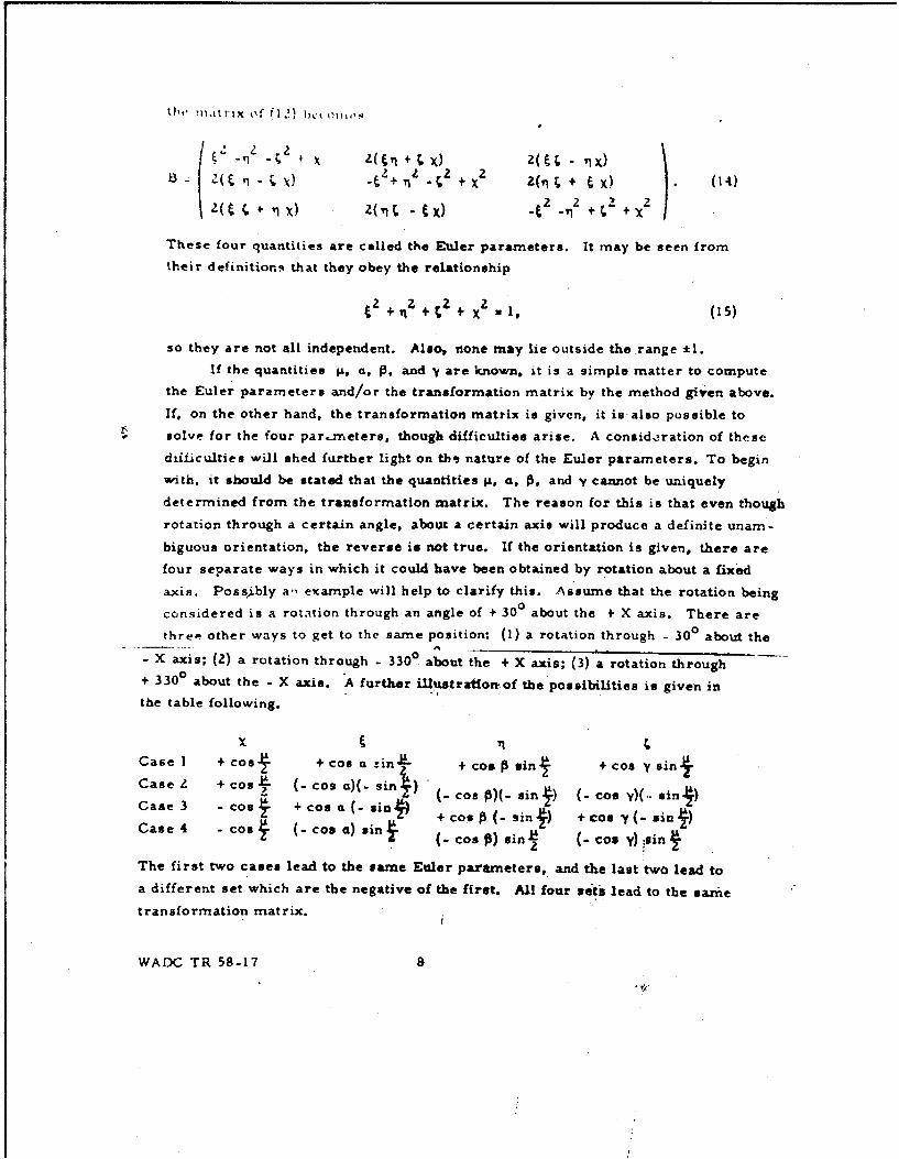
ma, ,~ trix of 02.) 1"" m ,,,
•':X -t -' l×Z(, + ;. X) n(• -'X)e=+ Y(n-.x - +, -• + X2(,1 + 4 X) (14l)
U~~ ~ Z~. 2 2x (i( xn .ix) Z(,• -x) +2 t +• J
These four quantities are called the Euler parameters. It may be seen from
their definition.si that they obey the relationship
2 z 2 2+q + z+ x=, (15)
so they are not all independent. Also, none may lie outside the range *1.
If the quantities ý&, a, P, and V are known, it is a simple matter to compute
the Euler parameters and/or the transformation matrix by the method given above.
If, on the other hand, the transformation matrix is given, it is also possible to
solve for the four par.meters, though difficulties arise. A consideŽration of these
dLficulties will shed further light on the nature of the Euler parameters. To begin
with. it should be stated that the quantities I, a, A, and y cannot be uniquely
determined from the transformation matrix. The reason for this is that even though
rotation through a certain angle, about a certain axis will produce a definite unam-
biguous orientation, the reverse is not true. If the orientation is given, there are
four separate ways in which it could have been obtained by rotation about a fixed
axis. Possibly a- example will help to clarify this. Assume that the rotation being
considered is a rotation through an angle of + 30 about the + X axis. There are
three other ways to get to the same position: (I) a rotation through - 300 about the
- X axis; (2) a rotation through - 330° about the + X axis; (3) a rotation through
+ 3300 about the - X axis. A further ilUustrattorwof the possibilities is given in
the table following.
x '1, r
Case I + coo~ + Cos CL -in.~ + coo * in ~ + coo y sin~Case Z + coso (-+cos a)(- sin•) ' ( si• (-cos y)(.- sin.)
Case 3 Cos~ +Coo a(L -sin.~ + coo (sin) + cosy(sin)Case 4 -Cos~. ( cos a) sinf P-cs~ in -csy 1 )i~
The first two cases lead to the same Euler parameters, and the last two lead to
a different set which are the negative of the first. All four Vets lead to the same
transformation matrix.
WADC: TR 58-17
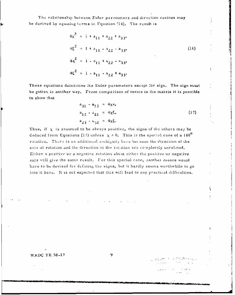
The relationship between Euler parameters and direction cosines may
be derived by equating terms in Equation .14). The result is
"4X = i + aI + aZ 2 - a 33,
4g 1 + a a
4x =1-a 1 1 +a 2 2 +a 3 3 '
4 2 l-a -azz -+ a(1
These equations deter~n-ine "-he Euler parameters except !or sign. The sign must
be gotten in ane-ther way. From comparison of terms in the matrix it is possible
to show zhat
a 1 a 3 3 ,T~
a31 -a. Xq
12
Z3 2=
Thus, if X is assumed to be alw a ys positive, the signs of the ethers mnay bededuced from nEquations (17) unless P m0. This ex the special caTe of a 180m
rozatuon. Tcra is an additi.oi,,m.1 •JUhU liv huc 1vvLiuu• the 6~irectior of. theabes of rotation and the direction co a the rottion are cterm pletely unrelated,
Eizlher a positive or a negative rotation about either the positive or negativet,%,ill gve the saoe result. Yor this special case, anotheih aneans would
have to be devised for dcpsLnitg tht signs, but it hardly seems worthwhile to go
ihvto it herv. It is nft expected that this will lead to any practical wifficultios,
WAIDC TIR 58-17 9
.......................... -'.-- .. "-....T' .....
- J'•' ' •,,a~ -e
--. •. : - . - •, , - .': ' ,. -
SECTJON III
"T I E C.AYfLEY -KLEIN PAIRAMETERS
In this development of the four-parameter system, it is found that a
2x2 connpltx initrix mnay b't used to represent a real rotation, rather than a
3>3 real nmatrix, Consider such a matrix (H) 0 iI
Ih I hlz
(H) = (18)h21 h22 1
"ifhe i-equtreinent is placed on this matrix that it be unitary, that is to say the
prcduct of (11) and its adjoint must yield the unit matrix. The adjoint is the
complex conjugate of the transposed matrix. In addition, it is required that
the determinant of the xnaL-ix (It) have the value +1. The unitary condition
allows t1 for the determinant, so this is an additional requirement. The
unitary condition may be written as
(xu: hx:) C1 t is = 1 • (19) 1
1hl2 h 2 * h Zl h z 0 1
Lxp:d~iJg and equating components gives
hlI *hII + h b *h = 1,
hI 1 *h 1 2 + h 2 1 *h 2 2 0,
hb1 2 *b•1 1 + h 2 2 *1>- =0,
h *h +b, 2 *h2 =1.
"The sfecond and third equations are the saine, being mnerely comnplex conjugates
of each othir. The first and fourth equations have no-imaginary con-onent,
\vhireas the second (or third) has both real and imaginary part--;. Therefure, the
three independent equations contain four conditions. These, together with the deter-
sninant requirement that h 1 hII - h 2.1 h z = +1 make it possible to determine certain
relation•ships an-iong the four quaiitities h1n. It may be shown that hI = hI*
and hil - h s . o 1he i:1tlx. may be written as
WAY,; TR '8-17 10
....... nn."-
I hI hlz%1(H) = ( 1 1 (21)
I.h 1 2 * h 1 1 *
The quantities h III h 1 2 , h 2 2 are usually referred to as the Cayley-Kiein
parameters. It will be noted that they are complex numbers. While it is
convenient to use them as such analytical operations (and this is the
purpose for which Klein develcFed then:) a physical computer must treat
t-omplex nurnibers in terms of their real and imaginary parts. Therefore,
it is convenient to introduce fou- other quantities defined as follows:
*h I =e I + ie 2 ,
2+ iee 4 (z)
where the e's are all real numbers, and i is tne square root of -1. Using
th.se definitions, the matrix (H) may be written-j as
e +ie + ie
(H) I (Z3)te3 +ie4 eI - iej
Now consider another complex matrix (P), which has the form
z x-iy(P) (Z4)
X+-z ) z
where x, y and z are real numbers. It will be noted that the matrix (1') is
equal to its own adjoint, and thus is said to bc self-adjoint or Hermitian. Now
consideir a transformation of (P) of the form
(F)' = (H)(P)(-H)+ (as)
where (1)+ designates the adjoint of (Hy. Since (IH) is unitary. (H)"- =(H)-
f so equation (Z5) is
(M)' = (26)
This is a similarity transformation. It ia shown in Appendix A that the deter-
,rinant of a matrix is invariant under a similaxiiy tra.,formation. It can also
be shown that the Hermitian property and the spur are both invariant under a
VWA LO3 TR 58-1? 1-
. ...- _',_ --- • * • • , , . .•,_ .: w, .4k. • .,! i,
Ssi-,ilaxity trahsformation. Therefore, the transformed natlix (P)' must
Shrvc the lormJ X' - ly'
ft I *S( )-= .( T
* t iy' -Z
4 The fact that the determinant of (P) must equ;,± the determinant of (2)' gives
|x +y + z =x +y +z' Z (28)
If x, y and k; are viewed as components of a vector, then Equation (28) is the
requirement that the length of the vector remnain unch*,iged. ZEpiation (26) May,
be: written
M -ey -3 Cy et + z e-ie - ie
3) 1 1if the operaiati ic (29) a:Ie carried out, it is found that
!a
!~ z _e 2 ,Sx• ( e z e3 + C 4-)x _ 2ýC-Ie ez + C 3e 4)y •-2('e,'4 e, '3)
y C = + 2 -( e e 4 -Jy + 2(e e(30), 4 1 2 e4Z
', (e e 3 + e(I 4 ) x + z(eC,% C ee.)y + (e' + e 2 23~~0 -40 1 a 3 - 4 ]z
lhu.e equations represent a linear transfurnmation between Jte components of x. y
1 and z, and the components of x' Y' and z'. The matrix for this transformation
e 2 e2e2 3Ie2 e4 2(e4e4-e)e4 )
L) CC +e4 '31)'' 24 3( ' 2e.- e 110 2 2 2e,, )
* 4e1 1 - 2 '[3 4 ¶ 2 3 Tt 4 t 1 .~S""
2 2 Z )Z(e1 e 3 4-e2 14 ) 2(e 3 -e, C) e ze Ve3 4
It may be shown directly that this matrix satisfies toe orthogonality conditions,
but it is proved :ls,, irom Equation (28). Equation (31) shows, that the nine
.ir'c cines ay be exprested in terrni of the four e.-; If Equations (Z )
W A C TR 5$-.A7 lZ
S ... ... ...... . i .. .. • n | | | | (
r.0 ,ailutt td tnto E-quaut)nb (-MO) it is fouud that
e 1 + %3 +4 (04
and therelore, only three et the a'# *r* !.Adqpendent. The identity of theec
four quan~itifta with the Euder paramgeters is obvious. Comparicon of EquAtions
(31) and (14) gives
aL X• z={. '.3 =. 4 4 , (33)
An equivajence has been indicated bewqen the prs! (3x3 ) matrix (A) and dhe
comlplex (2.4Z) mnat'ix 0j). it may be shown that this correspondence goes
further. Consider the real transforuatit-n
. , . . ... (34)
aci let the aesociated unitary complex matrix be tH)It ao that
(P), (H(R)(H)r (3r,)
Now consider a secorid transform~ation (A) with associated (H) 2 .
',, ý (A)-',
(P), = (H)z(P),(H)" , (36)
Sabstituting (34) and (35) into (36) gives
Therefore, if (A)(B) ,rC) and (H)z(H), =(H)3, the above eKutions become
'Ing .h-t multiplication of two rea 3-z3 W atricee correspWU4s to mr-ltip•icatron
of the twu associated Zxz complez matr'ices ir the a,•-ne order. Two types of quan-
titios which cor:espond in this Manner are E4id to bts isryorplhtic.
WADC TK 5B- 1 7 13
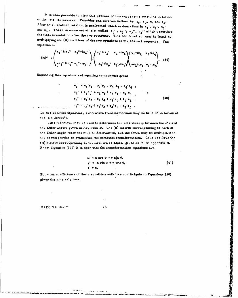
It s also0 possible to view this prVc#o o! two *tccesosve rotatitun in termcnof th e e'a the..gc ~ve. Consider one rotation deftned by of. e1, e 3 and e4 .After this, another rotation is pertornmed wLich im desecribed by Is', *'" t'3and a4'. There it solins set of ens cka4 elled e2', e3,1". u.4" wl-Ach describesthe final ortnz,tation after the two rutifons. TiLd conhlnc-d sot may b, found bymultiplying the (H) n'atrices of the two rotatioas in the co:,ract sequence, The
equation i&
/ ~~ ~ " .1. (39) ~ie 3 + 5
(a) 31 (e Q'ih01.iez" 3 4e" )14 11-1 ý1i I
Expanding this eqtvation and equtttinj companente gives
till" t t 'e - - 3' @ 3 - 44 "4
7" 1 e%, ' 4z el 'Sj ÷ e 'I + 0 3 'ti %4 t3
03" O'e3 - 02"04 t"3'el +÷3 44 0Z (40)
C 4 " t jZe 3 + *1 It4 4- j4'e l .. I3 1ez
13y usue of these equLations. succeshive transformations may be handled in terms ofthe e's Eirectly-
This technique may be used to determnina the relationship between the eta andthe Euler angles given in Appcndin B. The (1) matrix corresponding to each ofthe Euler angle rotations may be. detor.nined, and the three may be multiplied in
the correct order to synthesize the complete transformation. Consider first the(t-t) matrix correspv'ndir-g a.'to t raf i crr..- - -- gien 3! 'C' in A.pdir R.F, am Equation (179) it is seen that the transformation equations ar•e
y' =. -A sin 4 + y cea4 (41)
£3quating coefficients of these equatiOv.a with like coOefikcirtS in Equatil (0)
gives the nlne relations
WADC TR 58-17 14
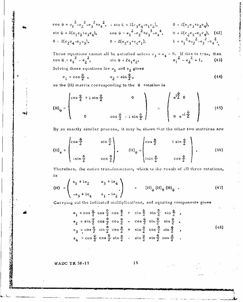
= 2C _e3 - sin 2 = (e 3 e 1 -Cel)1 0 Z(el e 3 4c 2 e 4 ),
sin , = Z(e e 4e 3 3 e4). Cos C - 1 e 2 3+e 4 Ze 43 l (4z)
-. 2(eC 4 -e ee+2 0 = 2(eCe3 +Ce), C C I 2 2e3 4
These equatiuns cannot all be satisfied unles;s e = e4 C 0. if this is true, then2 2 3 42
cos t'.= eC - S2 , Sin z 2ceC , e e (43)
Solving these equations for e1 and e. gives
eC cos e sin', (44)
so the (H4) rr.atrix corresponding to the 'b rotation is
COS + in t 0e
(H)r (o +i (45)i si'iL0 COS5-7 01-
By an exactly similar process, it may bu shown that the other two mnatrices are
sinjCs\ si
-sin Cos isin 4 cos (4-
Therefore, the entire transformnation, which is the result of all three rotations,
is
(1H) = : = (H)ý (H)e (H), (47)-3. 4 i -iZ
Carryixg out the indiicated a,"l ,.l-,Qg and enuating components gives
de cos cos - Cos + sin sin sin2 2' z
e 2 =sinz cos- COSz - COS osl-- s5n 2
e cos sin 2 cos + sill COs - sin (48)3 2 2 2 z
CoB c os sin• - sinl sin- cos?'
WADC TR 58-17 15
C. .. ... ... _____ 0
SECTION IV
QUAT ERNIONS
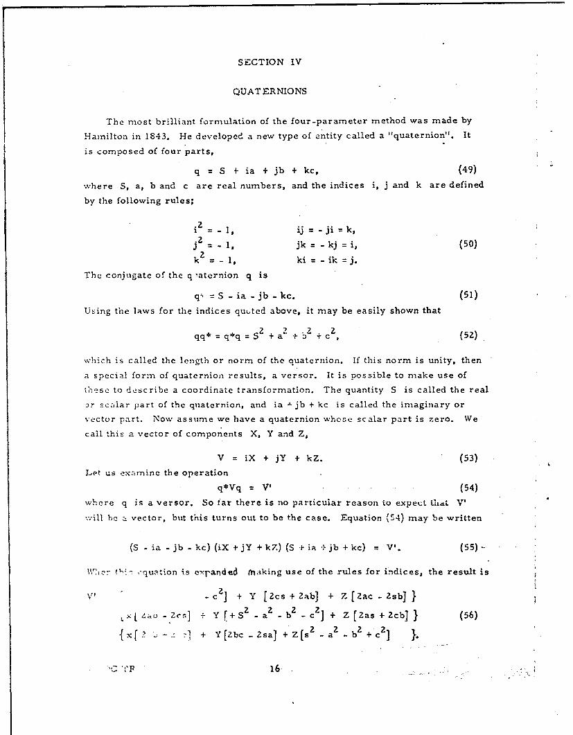
The most brilliant formulation of the four-parameter method was made by
Hamilton in 1843. He developed a new type of entity called a "quaternion". It
is composed of four parts,
q = S + ia + jb + kc, (49)
where S, a, b and c are real numbers, and the indices i, j and k are defined
by the following rules;
.Z1 = - I, ij - -ji =k,2j =-, jk =-kj =i, (50)
k= -1, ki =ik =j.
The conjugate of the q aternion q is
q;, = S - ia - jb - kc. (51)
Using the laws for the indices quted above, it may be easily shown that
2 2 .2,Zqq* = q*q = S + a + c ,(5)
which is called the length or norm of the quaternion. If this norm is unity, then
a special form of quaternion results, a versor. It is possible to make use of
.hese to de2scribe a coordinate transformation. The quantity S is called the real
Dr scz.lar part of the quaternion, and ia 4- jb + kc is called the imaginary or
vector part. Now assume we have a quaternion whose scalar part is zero. We
call this a vector of components X, Y and Z,
V = iX + jY + kZ. (53)
Let us examine the operation
q*Vq = V' (54)
where q is a versor. So far there is no particular reason to expect th- t V'
w,,ill be a vector, but this turns out to be the case. Equation f'4) may be written
(S - ia - jb - kc) (iX +jY +kZ) (S + ia +-jb +kc) = V'. (55)--
\,.•.?- 0-7-quition is exranded Mraking use of the rules for indices, the result is
V1 -c] + Y [Zcs + Zab] + Z [Zac - Zsb] }
+ Y[S -a.-b C] Z[a+c} (56{ xf?: :-1 + Y[Zbc - Zsa] + Z[s2 - a- b2 + C] }.
16-
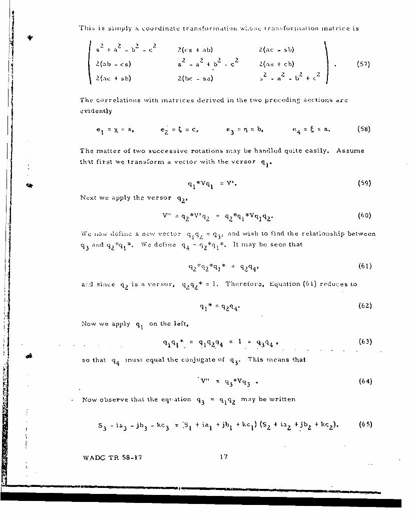
ilThis is simply a coordinate transforinat-.)n wl.i, nra::.furxnatjOn matrice is
S .a - c. 2(cs i ab) Z2(ac - sb)(a )s2 -a2 2 . C 2as + cb) €7
2(ab-+cs) s - bZ - c (5)
2(ac + sh:) 2(bc -sa) b
The correlations with mnatrices derived in the two preceding sections are
evidently
e1 = Y -- s. = r -c %: =b = C , (sejxs, ez=c ey3 b, C 4 ~a (58)
The matter of two successive rotations miay be handled quite easily. Assume
that first we transform a vector with the versor q,.
ql*Vql V'. (59)
Next we apply the versor %,
V" = q2 *V'qz = qZ*q 1 *Vqlq 2 . (60)
1VeiiU J:,,ýi•c a nevw vect qiq, : q 3, and wish to find the relationship between
q3 and q2 *ql*. We define q4 = qz*ql*. It may be seen that
42 *q2*ql* = q2q4, (61)
a~.d since q 2 is a versor, qzq 2 * = 1. Therefore, Equation (61) reduces to
qj* qZq4" (62)
Now we apply q, on the left,
qlql* 4 qlqg94 = 1 = q3 q4 , (63)
Sso that q m ust equal the conjugate of q 3 " This means that
V" q 3 *Vq 3 . (64)
Now observe that the eqi ation q3 = qlq, may be written
S 3 - ia 3 _jb 3 kc 3 ',SI + iaI + jbI + kcI) (SZ 4 ia 2 . jbz + kcz). (65)
WADC TR 58-17 17
m a m na
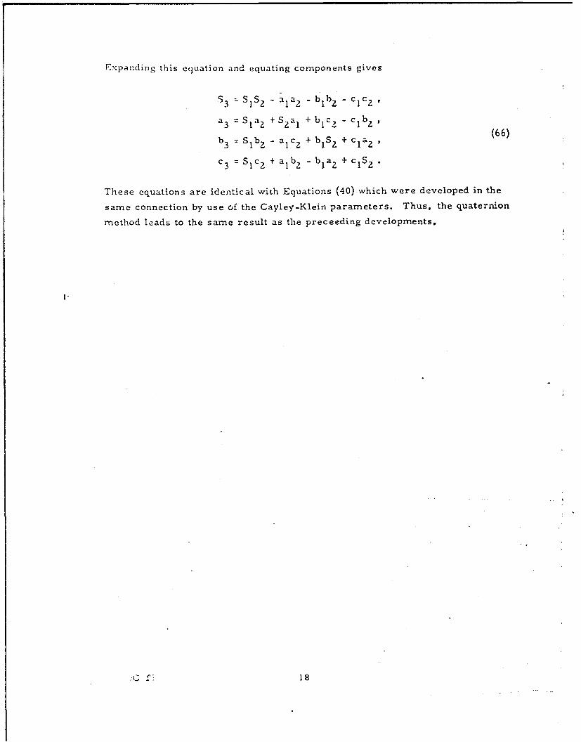
Expanding this equation and equating components gives
93 -- S2S - a1a2 - bIbz - c I cz
a 3 = SIa 2 + S2 a1 + bIC? - c 1 bz
(66)b 3 =Slb - alcz + b1 S2 + cla
c 3 = SIc 2 + a1b2 - bIa 2 + clS-
These equations are identical with Equations (40) which were developed in the
same connection by use of the Cayley-Klein parameters. Thus, the quaternion
method leads to the same result as the preceeding developments.
I-
.G r: 18
"SE"CTION V
INFINITESMAL TRANSFORMATIONS AND RATE- OF ROTAFION
The preceding sections have dealt with the four-paralr;2ter nt.t0hod Of
specifying the orientation of a coordinate s~fstein. As wa stated in Suction 1,
however, the primary interest is in determining the orientat0on from the rate
of rotation through a process of integration. Accordingly, it is necessary to
relate the rates of change of the four parameters to the rates o0 rotation of
the axis system.
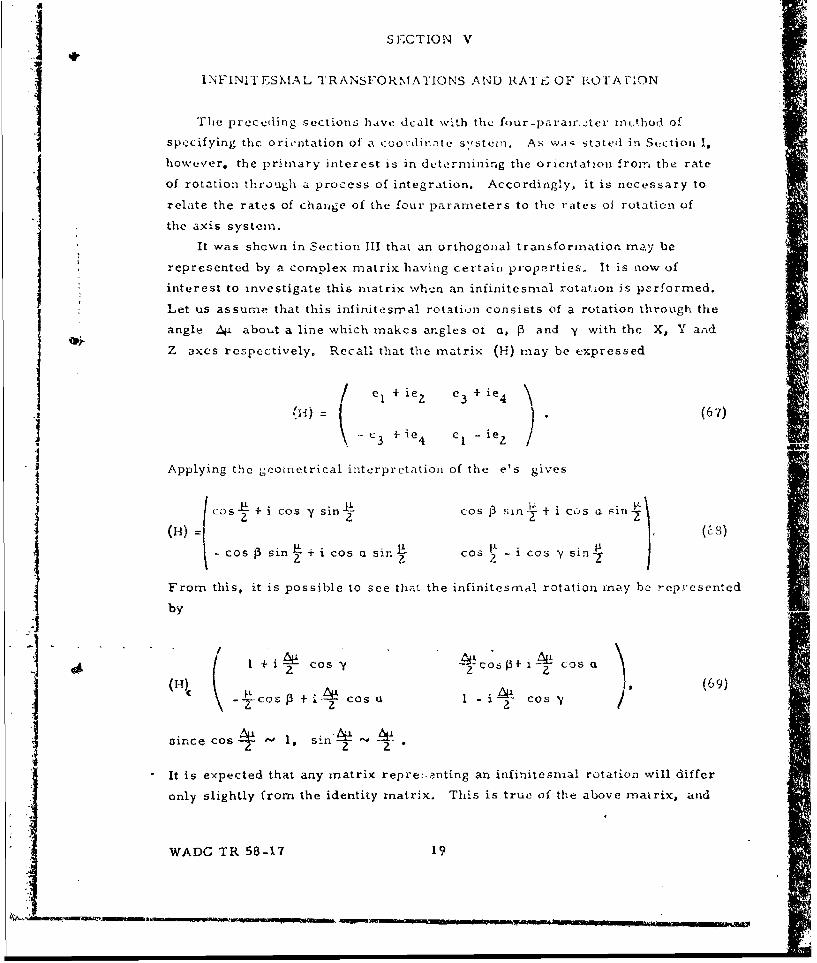
It was shewn in Section III that an orthogonal transformation may be
represented by a complex matrix having certain properties. It is now of
interest to investigate this matrix when an infinitesrnal rotation is performed.
Let us assume that this infinitesmal rotation consists of a rotation through the
angle 4.1 about a line which makes angles ot a, fP and y with the X, Y and
Z axes respectively. Recall that the matrix (H) may be expressed
e a + ie e 3 + ie4, ,30=) .(67)
.. c3 + ie 4 C - ie z
" I Applying the geometrical interpretation of the e's gives
ao-`L+i Cos Ysintý-csPsnL o i
Co Psin --L+i Cos asin- LL Cos t mE - iCos - sinl2(3((: 4-- sn (6 )
From this, it is possible to see that the infinitesmal rotation may be represented
by i eso
I' +o C + : cos Q o i P- i -A-' Co(H)cos / (69)
I ~ since Cos r2 2 ~~
It is expected that any matrix repre'.enting an infinitesnial rotation will differ
only slightly from the identity matrix. This is true of the above matrix, and
WADO TR 58-17 19
- 3aahlm.Mina.~a~,V:
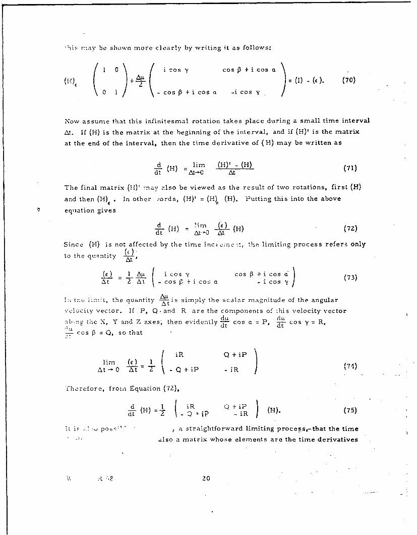
'nis r--av be shown mnore clearly by writing it as follows:
1 0Si cos - osP+i Cos a
( ( : +(= (I) - (C (70)0 1 -Cos P3 + i Cos a -i Cos Y
Now assume that this infinitesmal rotation takes place during a small time interval
At. If (H) is the matrix at the beginning of the interval, and if (H)' is the matrix
at the end of the interval, then the time derivative of (1H) may be written as
d lim (H)' -(H) (71)dt (H) At
The final matrix (H)' -nay also be viewed as the rcsult of two rotations, first (H)
and then (H), . In other ,ords, (H)' = (H)F (H). Putting this into the above
equation gives
d ( ) = im ( (H) (72)
dt At7-0 At
Since (H) is not affected by the time inccmc.-, the limiting process refers only(E)
to the quantity -A-,
_r I AU Cos y Cos P +iCos a" (73)At 2 At -cos +i cos a icos y
th in.-t, the quantity N'tis simply the scalar magnitude of the angular
velocitv vector. If P, Q . and R are the components of 1his velocity vector
.!,.ns the X, Y and Z axes; then evidently-du Cos d =P, g• cos y=R,
cos f = Q, so that
SiR Q + iPlir (E) 1 -At -- 0 ,-'"A T 2 Q + iP - iR '
fhorefore, froin Equation ('12),
d-t (H) =R Q + -i iR (H). (75)
it Ss .. , pos;:" , a straightforward limiting proces.s,-.that the time
also a matrix whose elements are the time derivatives
t ,20
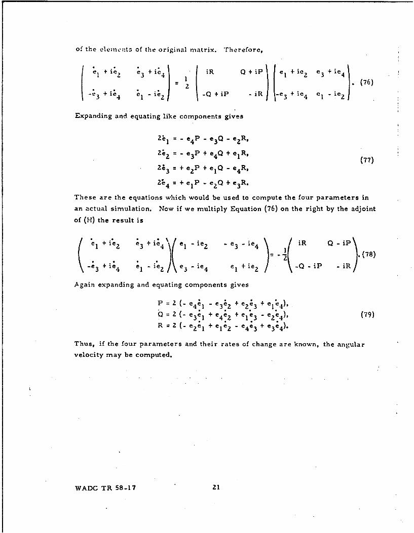
of the elecnlt. of the original matrix. Therefore,
I + ;e +ie4 iR Q +iP I + ie2 e 3 + ie4"= I (76)-e ie; e i;? -Q + iP - iR -e3 + ie4 eI -ie2
Expanding and equating like components gives
eI= e 4 P -e 3 Q -eR,
2e 2 =e 3P +e 4Q +e 1 R (77)
2 3 =+ e2P + elQ -e 4 R,
2 e4 + eIP - ezQ + e 3 R.
These are the equations which would be used to compute the four parameters in
an actual simulation. Now if we multiply Equation (76) on the right by the adjoint
of (H) the result is
e + i 2 ; + i; 4 e l -ie 2 - e 3 - ie 4 iR Q -i p \ . 7 8
-e3 +ie4 e1 - ie e3 ie4 e 1 +ie 2 -Q - iP -iR
Again expanding and equating components gives
P = Z (-e 4 ; 1 - e 3 2 + e 2e3 + e1e 4 ),S= Z (- e3ý1 + ee4 2 + e1* 3 - e 2 4)p (79)
R=Z(-eze1 +ele 2 - e; + e 4 ).
Thus, if the four parameters and their rates of change are known, the angular
velocity may be computed.
WADC TR 58-17 21
SECTION V1
THEORETICAL ERROR ANALYSES
in the preceeding sections, the fundamentdl theory of the quaternion
method has been pcesented. Before proceeding to an application of the
method, it is of interest to study theoretically the errors to be expected.
Not only w.vill this give a prediction of the results to be obtained in the
simulation, but it will give a better understanding of just how the equations
must be instrumented in order to achieve the maximum accuracy of which
the computer equipment is capable.
As was mentioned earlier, both quaternion and direction cosines will be
sir±-ulated, so errors for both were analyzed on much the same basis. It is
felt that this is an inipurtant part of the demonstration, because without a
theoretical error compari on, any differences found in the simulation would
be subject to the question o computer malfunction. If simulator results and
theoretical error analyses agree with each other, the degree of confidence in
the comparison will be much higher. Theoretical error analysis is but little
used by analog comnputer operators, especizaly i.-i non-linear problems such as
this. It turns out, however, that both quaternions and dir.-ction cosines lend
themnselves readily to an analysis of errors and the results obtained agree with
observations.
A. Direction Cosine Method
The fundamental equations to be used in generating the direction cosine
tr,;sforrnation are given in Appendix A. There are, however, m•any possible
variations which will be discussed briefly. Possibly the most straightforward
way would 1-e to solve the nine simultaneous equations and thus generate all nine
o' ;:ae direction cosines by integration. As the solution progresses, however,it is inevitjulie Uhit errors will l-c'-"u-"ula'. s,, Ue ofel J ,L±1 1- U ,
si;ch nature as to cause the orthogonality conditions (Equations 130) not to besatisfied after a time if, indeed, they were satisfied initially. This may be
thought of as a departure of the three axes of the nmoving system from mutual
orthogonality and distortion of the unit It-n-th of these axes. Some of the errors
-ri.::g 'n t-e sol-,:t:ton will r-" ccatj-=bute to this, and these may be thought of as
tnAL,%.i drift , the coordinate system will drift as a whole, and
W 3 -22
in addition, the unit vectors will change their relative orientations and lengths.These last two difficulties may be eliminated, as will be shown presently, butit should be understood that this is of but little value unless some way can befound for making the drift of the system as a whole tolerable. In an aircraftsimulation where a coordinate conversion is used, thcrc generally exists somefeedback which will eliminate long-term drift in the coordinate system. As willbe shown later, the drift can be reduced to where it is much less than those drift-producing elements in the physical system bcing simulated, such as airframemisalignment, gyro drift and amplifier noise. If the errors due to rotational driftcannot be corrected, there is not much additional penalty in accepting the errorsdue to non-orthogonality. In any case, it is advisable to determine in advance howmuch drift can be allowed in the given application, and to design the coordinateconversion to meet the requirements, using the techniques developed in this section.
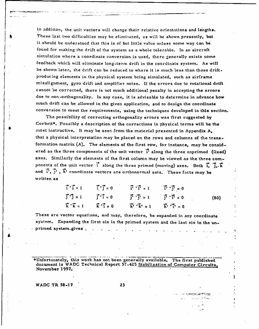
The possibility of correcting orthogonality errors was first suggested by
Corbett*. Possibly a description of the corrections in physical terms will be themost instructive. It may be seen from the material presented in Appendix A.that a physical interpretation may be placed on the rows and columns of the trans-formation matrix (A). The elements of the first row, for instance, may be consid-
ered as the three components of the unit vector i" along the three unprimed (fixed)axes. Similarly the elements of the first column may be viewed as the three com-ponents of the unit vector i along the three primed (moving) axes. Both i, j,.k
and i',J - k' coordinate vectors are orthonormal sets. These facts may be
written as
-4- .-4
S= 0 i 1 i ' 80)k k I~ k 0 k' "-'k' 1 kv ", = 0 (0
These are vector equations, and may, therefore, be expanded in any coordinatesystem. Expanding the first six in the primed system and the last six in the un-
Sprimed. ayst-em.gives - .
*Unfortunately, this work has not been generally available. The first publisheddocument is WADC Technical Report 57-425 Stabilization of Computer Circuits,November 1957.
WADC TR 58-17 23
2 2 2
all + a 2 1 + a 3 =31
2. 2 2
a 13 + a +aZ + = 1,a 23 + 33=,
a 1 a1 2 + a21.a2 2 + a 3.a 3 2 = 0,
a11a13 + a 21a2 3 +a a = 0,
a 1 za 1 3 + azzaZ3 + a 3 Za 3 3 = 0,
(81)2 zZ 2
all1 + alI + a 13 = 12 2
a 1 +a +a 2 = 1,
2 z 3a 1 . +a +.a3 = 1,
a3 + a + a =3. 32Z 33
a11a21 + a12,22 + a13a23 -,
aIIa 3 1 + a2a32 +a a 13a33- 0,
a21a31 + a 2a32 + a3 a33 0.
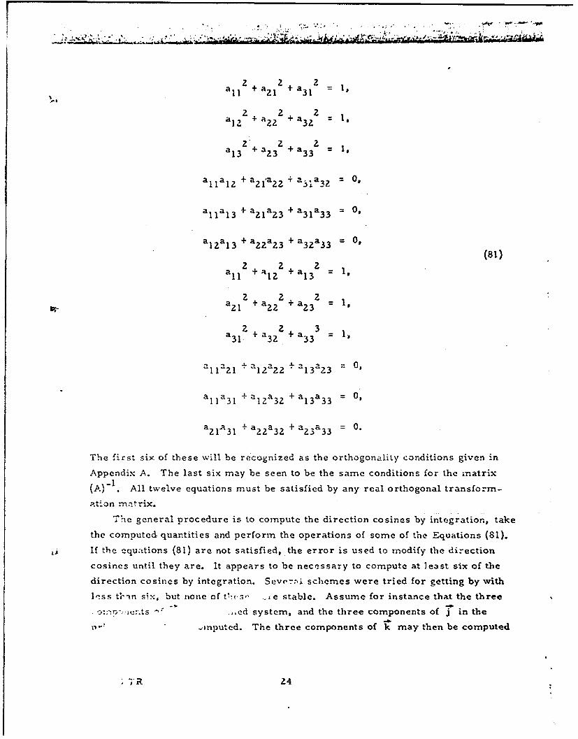
The first six of these will be recognized as the orthogonality conditions given in
Appendix A. The last six may be seen to be the same conditions for the mnatrix
(A)- 1 . All twelve equations must be satisfied by any rcal orthogonal transform-
ation matrix.
he general procedure is to compute the direction cosines by integration, take
the computed- quantities and perform the operations of some of the Equations (81).
If the equations (81) are not satisfied, the error is used to modify the direction
cosines until they are. It appears to be necessary to compute at least six of the
direction cosines by integration. Seve";ýi schemes were tried for getting by with
less t--in s-:-, but none of tl:es- .xe stable. Assume for instance that the three
'.,cd system, and the three components of J in the
... .nputed. The three components of k may then be computed
T 7R 24
without integrations from the relationship that k =-ixj. If six direction cosines
14W are computed by integration, then three of Equations (81) must be used to
eliminate redundancy. If nme '--sines are integrated, then six auxiliary equations
must be used. Both possibilities were proposed by Corbett*, and an improved
version of the second by Howe**. The first alternative (called the two-vector
method) was the one chosen for use here. It was selected because it uses less
simulation equipment, though the advantage over Howe's three-vector version
is not great. Both require 36 multiplications, though the two-vector method
requires only six integrators rather than nine.
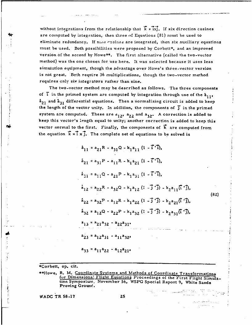
The two-vector method may be described as follows. The three components
of "T in the primed system are computed by integration through use of the ýl
and I 3 1 differential equations. Then a normalizing circuit is added to keep
the length of the vector unity. In addition, the components of " in the primed
system are computed. These are a12 a 2 2 and a A correction is added to
keep this vector's length equal to unity; another correction is added to keep this
vector normal to the first. Finally, the components of k are computed from
the equation k = i x j. The complete set of equations to be solved is
Aa21 = R - a a - a
1a 2 1 P "ka 31 (1 -0 "),
l ---aR - a 3 2 Q R klal 2 (1 --a" - k~a1 l( 1),
& 2 2 = a 3 2P"a 1 2 R " a2 (1 -a ') - kka 2 ".(
a32 =a - a42P - k3a 3 1 1 -- j) -kza i'j),
a 1 3 a 2 1a3 2 - a 2 2 a 3 1*
a 2 3 =a 1 2 a 3 1 a al32-
a 3 3 =a 1 1 a 2 2 - a 1 2 a 2 1,
*Corbett, op. cit.
**Howe, R. M. Coordinate Systems and Methods of Coordinate Transformationsfor Dimensional Flight Equations Proceedings of the First Flight Simula-tion Symposium, November 56, WSPG Special Report 9, White SandsProving Groune.
WADC TR 58-17 25
where. 2 2 2 -. 2 aZ 2
I +-a11 ' I2 + a3 1 J a IlZ + +a3Z
1 a a aa 1 2 + a 2 1 a2 2 + a 3 1 a 3 2.
It will be observed that there ire six differential equations, and three algebraic
equations, so that six integrators will be required. The k1 terms are for
correction of the length of the vectors and the kZ terms are to retain orthogon-
ality. The k1 and k are arbitrary gain factors which will be discussed later.
.It appears that the above method is a slight improvement on the version given by
Corbett in that the orthogonality. correction is added to only one vector rather than
to both. The entire drift about the z axis, then, is determined by the drift of i
alone. If the correction were fed into both vectors, the total drift would be higher
in cases where the two vectors tend to drift in the same direction.
The above equatior. are idealizations. The computer which is used to instru-
ment them will be solvii., approximations of these equations. The differences give
rise to errors in the solutions which will now be considered. For convenience,
all errors are divided into two categories, static and dynamic. The dynamic errors
are associated with the fact that the actual cqu,.tions the computer is solving are of
higher order than the ideal, and the static errors arise from .-rrors in resistance,
capacitance, pot settings, and the like. These two types of errors must be treated
by different means. The dynamic errors will be considered first.
It is assumed that the only dynamic effect of importance is the bandpass of
the multiplier. Amplifiers and integrators should be at least one order of magnitude
better than multipliers in this respect, so the assumption appears sound. A simpli-
fied analysis will illustrate the important issues. Consider the equations for com-
ponents of the vector i , with correction terms deleted.
a11 = a-,R - a31Q,
a2 1 = a 3 1 P - a 1 1 R, (83)
a 3 1 = a1 1Q - a?21P"
Now cc:.jider a s -al c cre P = R =0 and Q is a constant. These
.quatio
• rr.s•.,26
al I- a 3100
a3 1 = al1o, (84)
a., = 0.
If a2 1 is initially zero, it will remain so, and this equation may be deleted from
the set. If Q is constant, the remaining equations are linear. Taking the Laplace
transform of these equations, together with the initial conditions all 1, a31 = o0
and the result is
I Sa 1 a3 1Q,(85)
V Sa 3 1 = a1 1Q
If it is assumed that the transfer function of the multipliers is G(S), then these
equations would be
Sa1 1 = I - a 3 1 QG(S),
(86)
Sa 3 1 = a1 1 QG(S).
It is possible to solve these equations for all and a3 1,
S
"S + Q G(S)(87)
31 2S + Q G (S)
Before proceeding further, it is necessary to make some assumption concerning
G(S). It should be clear that for any reasonable result, this transfer function
should be only slightly different from unity. It must equal unity at very low
frequencies, *(static errors assumed zero). A reasonable assumption is that its
linear, i. e., in its power series representation the non-linear terms are negli-
gible in comparison to the linear term. We have assumed as reasonable
G(S) = 1 + T1S. (88)
WADC TR 58-17 27
Substituting this into Equations (87) gives
Sa1 11. =(S + TQ - +iQ)(S +t -iQ)
S Q(S + •) (89)a31 (S +- +iQ) (S +rQ -iQ)
Taking the inverse transform gives
a -TQt (cosQt -Q sinQt),
- TQ t (sin Qt -T Qces Qt). (90)a3 , e
' hese may be combined .o get the length of the vector,
a 11 +a 3 1 e- (1- TQ sin 2 Qt). (91)
Several conclusions may be drawn from this. If T is positive (corresponding
to a lead in the transfer function) then the length will decrease. If T is negative
(corresponding to lag), then the length will diverge. The term T Q sin ZQt repre-
sents an oscillatory error of p!,ak magnitude TQ. It will be shown later that the
amplitude correction term must be kept as small as possible to avoid angular
drift. Therefore, it will probably not be possible to get the-correction gain high
enough to cut down this oscillatory error term. The only way to keep it small
will he to keep TQ small. Let us assume, for instance, that a computing accur-
acy of 0. 1 per cent is desired. This means that TQ < l0"3. It may also be seen
that --Q is simply the phase lag (in radians) at the frequency 0. For the exa-nple
given, the phase lag at the frequency of oscil'ation should-be-less thinnne--nilli-
radian, or about 0. 06 degrees. The correction circuit will be able to take care
of the long term exponential ircrease quite well, though if the bandpass requirement
stated above is met, this source of -:r,)wth of the vector will be negligible compared
t! s".,- du2 to •t,- .rc .Vhich will be considred next.
TR 5 28
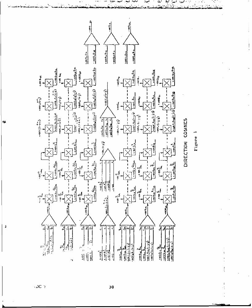
As a prelude to studying the effect of static errors, it will be useful to
consider a general symbolic diagram of the circuit rcsuircd to solvw the
equations. This is becauýe the problein of errors is inseparable from that of
scaling, so sonie sort of scaling must be assumed. This diagram i- given in
Figure 1. It may be seen that there are 36 multiplications, six of which are
independent. There are six integrators, six summing amplifiers, and in any
practical circuit, there would have to be a considerable number of inverting
and isolation amplifiers as well. As the nature and number of these depends
on characteristics of the multipliers being used, they are deleted in this
figure. A practical circuit for accomplishing this transformation will be
considered later. It is convenient to introduce a special notation for errors
in these multipliers. The voltage error in the multiplier which multiplies 100a 1 1
and 100-R is designated c 1R. It should be emphasized that this is the actualm
error in volts, not a ratio or a percentage.
Now assume that the multipliers have infinite bandpass, but do have static
errors. It may be seen from the circuit of Figure 1 that the equations for compo-
nents of the vector i are actually
a R a Q+K all (i-P-i)+Rn310 + B1 1 01 1 31 1m 100 m 100 C. 100 '
3,11-- E 1R KI EZiGa 2 1 = a 3 1 P -a 1 1 R+KIa 2 (1-i-i)+P m W1R Z1- E1C (9Z)S100 C 1 10(2
-_Q E__ IP 1 E31a a Q -a PK_ i 1 P31 11 211 131(-i'i)+Qm 100 m 100 C1 100
These are the equations which the machine will be solving. It is of interest to
investigate certain properties of the solutions to these equations, and to see how
they compare with the ideal.
First consider the effect on the length of the unit vector i . Assume that KI= 01
so that no corrections are neing introduced, The equations become
EZ1R _31QaI1 = a 2 1 R-a310 + R - n 100
-aP -aR + P P 1R R 93)
a21- 31 1 1 R- 1 R 100(E E£
a1 Q a +Q E IIQ p ZIPa 3 1 = a1lQ -a 2 1. 3 -+ m 100 rn 100
WADC TR 58-17 29
.. - .. . . ---- " '. - -I . . .. . •. _ . , I II I I _ III _ E
x~ ~ 7 a- X -4x
0 V1
~x x 7 1 6
cc I "Ic - -i 0 8
1*.- I-. - ', z
t; J .i
re 3J rLzfrE~H-v i
LI~IK30
"Th legt of byZ nd,,: diflý:Yentiatinl. thi sThe length of i is given by I = a1 1 a2 1 + a 31 f
expression with respetct to tinie,
211 -2a " +2 k + alIa 1 a 2 l~ag| 31 31
The length is close to unity for all cases of interest, so that, to the firt order,
I = a al1 + a2 1 a2 1 + a 31a 31 (94)
Substituting Equations (93) into this expression gives
EZIR E31Q E E1 R_15I = a1 1R 100 -a1 1 M 100 %a2Pm 210- a an R-100 1 (1
EI1 EZ+ a 3 1 Q 110 QP P zi
1 100 3 1 m 100
It is now necessary to consider the nature of these errors. In the first place,
the error is viewed as a random variable. For a given multiplier, the error which
exists is son-ie definite function of the two inputs. This function is more or less
repeatable, at least over a short time period, so in this sense it is not a randomn
variable. However, when one considers ciffc, ciiiL itiultih•iliers, g , -rror e.LIting
at certain valu?s of the inputs is now a function of which multiplier is used and is
thus a random variable. These variables are considered independent because
thete is no reason to expect that the error in one multiplier will influence the
error in another.
Two different types of error are considered in the subsequent analysis. In the
first type, called "uncorrelated", the error is assumed to be Gaussian and independ-'
ent of both inputs. In other words, the error existing at any given value of the inputs
it assuL±ed to be drawn from a normal distribution of zero mean and variance which
is independent of either input and of the particular iritultiplitr being used. This erro-
distribtuion is intended to be consistent with electronic multiplie'rs, though no propel4
statistical data are available on them. Usually electronic multipliers are adjusted
so that the error when either of the inputs are zero is somewhat smnvller than other-.
wise, and there are no data t(. support using a normal distribution. Until such data
are available the above hyp- theses are as good as any and more convenient than mos
vVADC TR 58-17 31
The second type of error, called "correlated" differs from the first in that
the variance of the errors is assumed proportional to one of the inputs andindependent of the other. This is intended to represent servomultipliers, andthe experimental justification here is somewhat better. Since this is the type ofmultiplier used in the simulation described later, the error distribution wasmeasured. Results are given in Appendix C, and tile normality of the distribution
is reasonably well verified. Proportionality of the variance to the voltage acrossthe potentiometer was not checked but it is an inevitable consequence of the nature
of servomultipliers.
The drift rate i of Equation (95) thus becomes a random variable. It is thesum of six independent Gaussian variables, so its variance is the sum of thevariances of the individual terms. Thus the standard deviation or square root of
the variance is given by
2o 2 2 a212 ,, 2 2 + 2 p22 [a R2 +a P +a Q + a2 1 R +a P (96)
e• i 100 11 Rm azI n 3 m a1M 31 ]½. (6
Cr. is the standard deviation of i and o- is the standard deviation of multipliererrors. It is not possible to evaluate this expression without knowledge of theparticular Pro, Q and R involved, but it is possible to determine a conveni-
m= 2O + RZM= f m r+ "
Making use of this fact together with the normality relation a + a2 +a 3 = a ,
it may be seen that
S• < ' .2- W' (97)
1 100 M (7
In the foregoing, errors of the first, or uncorrelated type have been assumed.
The drift rate tends to be proportional to the full-scale velocity, regardless ofwhat -velocity-actually exists; -- .. . .. ..
This is not true with the second or correlated type of error. Observe that
each of the multipliers is used to multiply a direction cosine by one of the angularvelocity components, P, Q or R. Consider, for example the multiplier whichgenerates the first error term in equation (95); the one multiplying a1 1 by R.
WADC TR 58-17 32
- - -: .
If e direction cosine is pit unto the -'}iaft of thii servoinultiplier, and R.
is put across thie potent1ionnetur, then the error :5t,tndtrd dteviation will be
proportiontil to R. a-_ postul-xti'd iarlicr. This fact iiinay be stated as
, 0' Cy where eo t. cio (rIFIll
is the standard deviation of erirors att full-s.,:ale, i. e. , when R = R If the
other multaplic.tions are treated similarly, then it may be seen that
F-< (98)
This result is somewhat more favorable than that for the uncorrelated case,
The drift rate tends to be proportional to the existing rate of rotation rather than
the full-scale rate. There would be little difference between tl,e two if the rate
were near the mna-.mum most of the time, but this is not usually the case. In
fact in many simaul, -ions, the rotation rate is small rnost of the time, the maximum
rates being required only once or a few times.
It is now of interezt to investigate the effect of the correction scheme on this
lennth drift. Wa consiider firsi t', LdSC of uncorrelared errors, if Ile complete
Equations (792) arc sub:stituted in Eqiation (94), the result is
C)%R a 1 Q '3Q 3 . 3lP11 I IIii){a n 100 11lM 1760- azm 100
a1 I El 110Z1 "i1n10 31 0 n-7(- 31 in9
-a a .K ---- C ---- a-P (99)
S1000 r al 1 lc ~2llc 31 a E3 1 c]
II
tonsiuier the first term in this equation. Observe that i.i is simply .Z, If it
is a 3cl:ned that I = 1.0 + At, then 1 "-1.0 + ZA1, so that the first term becoines
-. K: LAf. The second term is the same as the length drift rate of Equation (95).
The list term is the drift rate due to the correction nnechanis-n itself. For the
prosenit, it is assumed that C 1 is large enough that thi s last tern: is negligible
with respect to the first two. We will return to this point later. With this
assumption, then, Equiation (99) hecoines
'21 R 31 - P 31P 1ka 1 It+ 0 a 1 R.. ,)I -il -1 - al 1Q 1 100 21 ni t00 " I 100
1 0 1Q-a 3 ZI P (100)
3 a]lC 3 1 10V
"P.IC 3?a ý
C I nrbinIg L4qu.It:uorr, 102) and (103), the limits on K are
S0- C C-_ .. -- _ <_ K <
Tihere are several differences for correlated errors. When I? R 0 % ,
then all errors will be zero, provided the velocity components have been put
across the mulliplying poitentiornetcrs as suggested above. Under these circum-
s•tances, the drift is deterimined by integrator drift, and is at least an Order of
n-agnitude lower than the drifts normally arising from multiplier errors. If.
lh.\v.ever the length tolerance is to be met under the largest allowable rates of
rot,ition, then the lower bound on K1I is the samne as that of Equation (102).
The iupper L. ,nd will disappear if the error Signal is put across the potentio-
nmeter in the ( inultiplications. In this case, the error arising in the mnulti-(-n 2 nplier would be o the order of e rather than of the order of W . The gain would
not hhave an upper bound len, except for the fact that integrators tend to drift
acrso eh mul...'tr the il inhg r p oaco..... aga.... gt vh preceeding s eic.
Next the angular drift rate wdll be considered, Even if the coordinate systeof
is kt-udt lowetOhal, thedre is Still the tendency a o s rin t in orientation, which comes
priocitionly from static errors in the multiplerbsa The components P, Q and R
The upeLthe -'udwlar dclocitvs in the rovirg system. If pt Qo and Re are. the
cme,:-onts in the fixed system, it (n; ui bI shown that
R + +a a
"0 lI 1laZIZZ a31a32
Re 0 al a I ? + a2?- a 21 + a 32 a31
n vth a + th + fac ao 12- 13 Z 3 32.a33
-P a " 4. t + a i.I
0 o 1al Z a 23 2 3 a 3 2,
Q • a "a +a a -,a ao' 1 23 2 Z 1 32 31Q a "I + a a + a a
-o lla3 21 Z3 '31 33
,Ar < 84-7 33
This is a first order differential equation for Al, the right-hand side or forcing
term being a combination of errors. As the errors change during the course of• .•,,4,,J'.•- a.,: .. •.,4 WU&f~l.s ' .,L• *,0 •-V d-O ".',.60#4 M& d,•J",s.4.,A;ý ?4&€• •'!J W., ' "., ". - ' ,- , ... .
a run, then the length error Al will change also, but for simplicity consider a
static case. If the coordinate system is not rotating, then all direction cosines
are fixed, and the right side of Equation (100) becomes a constant. Let us call
it u. This constant will have different values depending on the set of multipliers
used, and in fact the standard deviation of the values it can assume is given by
Equation (97). In the steady-state, Ai must be zero, and frorn Equation (100)
ZKI Al = u
The deviation in Af will then be given by
AU = K"oT • (101)- 1 KI 100r- Wm
S4 is fixed by the nature of the m ultipliers, WV m by the scaling requirem ents. K ,
may be chosen, however, to make w as small as desired. Conversely, the
required value of K is
WK 1 > M (10Z)
l00,17 "A1
It was mentioned that the third term of Equation (99) should be negligible with
respect to the first two. The reason for this is not clear from what has been
presented thus far, but it will be seen later when angular drift is considered.
Angular drift is determined by a similar equation, and it seems unreasonable to
allow the length correction circuit to contribute to the drift in angle when it can be
avoided, as will now be shown, by proper distribution of gains. The third term ofK
Equation (99) will have the standard deviation v , while the standard deviation
of the second is i Wm. If it is required that the third term be less than one
quarter of thc nccond, then
S(103)I 00C 400
C 1 4
which determines CI. once KI is chosen. This establishes the upper limit'on KI.
WADC TR 58-17 32b
Now substituting Equations (912) into the third of these gives
-R lP - a R i C a Z1R 31Qo - az 3 Q I3 3 R+{-i0(m - - a12t'm 10
100c [ a C + az fl + a 3 2 3lI " (105)
The first three terms represent the transformation of the velocity vector into the
fixed axis system. In other words, they represent the "correct" value of R . The0
remaining terms represent the error in Ro0 , or the component of the drift velocity
vector along the unprimed Z axis. Combination of the errors is similar to that
for drift in length. If it is required that the last term of Equation (105) be negligible
with respect to the others, then the standard deviation of drift rate is given by
0 m 100
01< w _ _ (106)
0 • 100
for the uncorrelated and correlated error cases respectively. Thus it appears that
the drift rate will be a constant fraction of full scale, for uncorrelated errors, and
will be a constant fraction of the angular velocity for correlated errors, The
conditions on KI and CI are the same as developed earlier, namely
C <u W ft (107)Ir. /TAI 4
The drifts in P and Q are substantially the same pruvidtU gains are; chosen
such as to make the drift contribution of the correction circuits negligible. TheS
case of K2 and C 2 is substantially the saone as for K1 and C 1 , and they should be
chosen in the same way.
Analyses of drifts in P and Q are done is much the sanme way and lead to
similar results.
WADC TR 58-17 33a
13. Oiate.ntk iOl Error A ,ialv,.'.s
The quaternion siniultion may be handled in much the same way. I tie
quaternioxi components are not all independent, and we may make use of the
relationship, ,2 2 2 4e 1 + e2 + e 3 +e 4 1 , (32)
2 2 2 Iin the same way that al + a 2 1 + a31 1 was used to maintain the length
of the unit vector. The equations to be solved are
2eI = P e$ - e - eR + Krei •
ee -eP + e 4 Q + e R+ Kr~e2 ,9
2e: eP+eQ-e 4 R K+e 3 , (108) e
24= e.P - e 2 Q + e 3+ R + K ,e
2 2* = -el�e e -e1 2 - 3 '4
T[hev bandpcts :reuiexnn i-olit r.ietoi s oniy one nct il 13 cvert: as -Ejia ror
direction cosiucs. This may be seen in several ways. Consider the equa-tions
above with Q constant and )i R K = 0.
_____+_l__12
+ e 1 C2,(109)
+ tel Q,32 I
4 - e. Q_2
For initial conditions, we assure e I= 1, 0=.ee4 O Under these
conditions, e and c .,xil recain zero and the equations become
2
1IWAIJG; ItB 53-17 34
Theme are identical with those treated in the bandpass study of the preceeding
sec.tion except that the irequancy is reduced by one half. The same conclusion
can be seen from the definition of ea, From Equation (33), aI = cos ý./Z, so
"while u is completing a full rotation, ýi/2 only movos through 1800. This means
that the servos which axe driven by the e's only move with half the speed of those
driven by the a's, for a given rate of rotation of the coordinate system. Conse-
quently, for a givers accuracy, twice as much phase shift may be allowed.
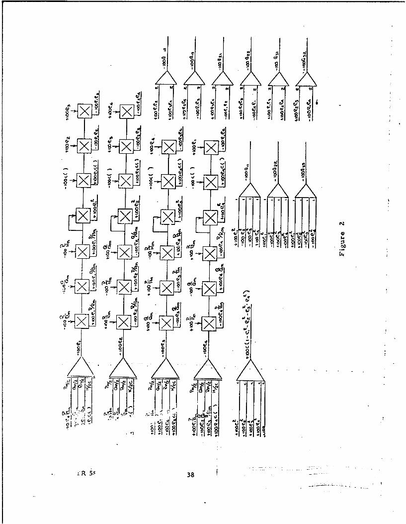
In order to analyze the effect of static multiplier errors, it is again necessary
to postulate somc particular scaling. The simplified diagram is shown in Figure 2.
The cquipment necessary for determining the direction cosines has been included,
as they wili always be needed. The basic quaternion component computation requires
Z0 multipliers and four integrators. Conversion to direction cosines requires
anothe." six multipliers, for a total of Z6 multipliers and 4 integrators, against 36
multipliers and 6 integrators for direction cosines. Notation for individual multi-
plier errors is similar to that applied earlier. The voltage error in the multiplier
which multiplies R and elV for instance, is called eIR' and so on. From this
figure, it may be seen that the equations being solved are:
'C -er 3 Z1.. *7-R K*~I Q~1 - 1 - ' -4P lU"J m i - Rrnuu 1 c Au "
-; 4 4 - P4•p I K QZc- 3 e4 Q 1 R e 100- m+Q 100o m 100 C 100
Z~3 =e 2 P +1 0 -~R in(O cl)
S+R K4e + Pn Q 4R!- K 3c3e z 2 I 1 •4. 3Ke + 1-0-0- •M 100 m 10--0" c 10--0
.~A + p P P "eL +-•-1 -+P pK "4c
2;' = + eP - eKiQ + e R +Ke + 00 i-" +c R
Consider. first the effect of errors on the length of the quaternion. The length
is given by IZ = el4 + 2 + e 3 • + e42 . Differentiating with respect to time gives
I= 4le .4 e-e, + e.• + -.Since the length is not to be allowed to vary much
f rom unity, the drift rate may be approximated by I ee + e05 + e e + ee.I I Z 3 3 4 4
Substltu.ng Equations (Il1) into this relation and performing the appropriate
reductions gives:
WADC TR 58-17 35
V.- . . . . . • - . .
I:
00- {-eiPnE4 P I rn (3Q - eIRm iZR " eZPm 3P
+ ezQm4 4Q 4 e 2 R cIR + C3Pm 2P + e 3Qr1 EIQ
~eR~ 4 +e P~ 4 -e 4 ( + eR c"3 in 4R 4 m IP - 24 rn 2Q 4Rm r3R
+ K { +--6÷e- + + 4c} (Ciz) eI OO I 0c c eCZ 3 3c 44c " "L-
If 1 z 1 + A, then the first term is simply - ZKAI. Thus Equation (lI2) becomes
Ai +1 K A - I 4P -' elQmC3Q - eRm - 'ZPmE3/• ~ ~ +e KRi t +"0 e Pe 4m4 +eQ a Z
S+e 2 Q 4Q + e 2 Rm •IR + e 3 P m + e3Qm rIQ
"e 3 R E 4 R + e 4 Pm fIP " e 4 Q iZQ + e 4 Rm •3R}
S200" e 1 t Ic + ez 2ZC +e 3 43c + e 4 a4 } (113)
which is analogous with Eq]uation (106).As in the preceeding section.. we assume the second term on the right of
Equation (113) to be negligible with respect to the first. The variance of the
first term is
zoo20O m
Thus, for the steady-state, (14a m(
=z, zoo oK11114.4• int.
where '41 is the standard deviation in the length erroi which will be allowed.
The standard deviation of the second terms of Equation (113) is -- a- . The
requirement that the second term be no more than one quarter the first gives
W
<4 C
WADC TR 58-17 36
Conibinini the two gives almost the same conditions on K as were obtained
fzi -the eirection cosine method.
'e W200 W' < K < C:
The foregoing is for uncorrelated errors. The changes in the correlated error
case would be the same as in the direction cosine analysis: the upper bound on
K disappears and the lower bound is the same as in the uncorrelated case.
Next the effect of multiplier errors on- the angular drift must be evaluated.
Equation (79) gives the rotation rate components P. Q, and R in terms of the
rates of change of the quaternion components.. The apparent value of P. which we
we call Pa is, the Pa = 2(-e 4 e1 - e3 e32 + aee 3 + e1 ; 4 )" If Equations (11) are
substituted into this expreasion, the result is
P (, +2 L +24 +a +e3 ee 4 )P + I- {e 4 (Pm 4P +Qm e30 M 2R)
+ae3 (Pm 3P -"m 440 - Rm IlR) + eZ(PmI ZP + 0 m Ila - Rm I4R) (116)
+ eI(Pro 41p - am ,,0 + R mI '3R) } + 1.--C{1' 4 '1c "e3'Zc +e, '3c + J
The first term is equivalent to ( I + Z2•)Pso the error in P. (P a- P) is
P =Pa-PsZ 2P I 10{e4(Pm"4P + 0m 3 + Ram 'ZR3 (117)
+ e 3 (Pm 43P a m I4Q " Rm 'IR) + eZ (Pm '2P + n %lQ - Rm "4R)
ei(Pm'iP " m ZQ + Rm {-R4 + l-e-e 4 'Ic e 3 2 c+ + 2e 3c + el 4c"
2,i is related to the choice of K. From E~uation (114) it may be seen that the
standard deviation in al is given by Ir. = 0-"•K Win. As before, we require the
last term of Equation (117) to be negligible. It remains to determine the variance
of the second term. By taking thi sum of variances of the individual terms, it is
possible to show that the standard deviation of the second term is I- Wm W 'i"
% 58-17 36a
Thus the standard deviation in AP is
= a, a W+ p 2
AP- 100 m --z-K 2
This is comparable to the value obtained for direction cosines if K is made
reasonably large.
Exactly analogous results are obtained for errors in the other two axes.
W5
WADCTR8-17 3
1 ty tV vi Nj N o
46, Qa
x7 x
X~ ~ x8 4d-' w tof
-. - .~w03 10
etc'l xIxc8I Cl - x ~ I
05~
N? x
.1.
0'1
5F3
SECTION VII
SIMULATOR RESULTS
The next step in investigation of quaterniori coordinate convec-tiion was
solution of the equations on an analog coriputer. The direction cosineO method
was similarly investigated, and an atte.mpt was made to make the conditions of
the two simulations as nearly alike as their inherent differences would permit.
Both were done on REAC Series 100 equipment. Servornultipliers equipped with
potentiometers of 0. 05 percent linearity were used throughout. The multipliers
were not specially calibrated for these simulations, so their adjustment was
consistent with normal practice in the Analog Computation Branch, Aeronautical
Research Laboratory. Of course, correct pot loading was used in all cases. In
both simulations, a maximum rotational velocity of 0. 5 radians/sec was employed
though scaling was such that P = Q = R = 1. 0 and both directions cosinesthogh calngwassuc tht rn rm m "
and the quaternion components were scaled so that 50 volts (out of 100 full scale)
represented the extreme I-ossible excursion of the variable. This was done to get
away from possible end effects on servomuitiplier potentiomneters.
Adequate checking of a coordinate convei :ion is a problem in itself, and while
it is riot claimed thai ite w .. ...tdoutdt: lJetf rt- st i-'-ex it.. .. r-s
sufficient, and no better method presented itself. With the types of coordinate
conversion considered here, there are two things principally to be checked: the
action of the "orthogonalization" or correction mecthanismns, and the rotation driftrate. The first may be checked simply by monitoring the error quantities which
are used for correction. The drift rate is not so easily checked, In most cases
the drift rate will be very small compared with the rate of rotation. An exception
to this is the case when an angular velocity of zero 3s desired. Any shift which
takes place under these conditions is readily detected. To chck the drift while
rotSting, the following procedure was adopted: a single input of P = 0. 500 rad/sec
(0 and R zero) was applied to the equations for a period of approximately 125.66
seconds. This is enough time for ten complete revolutions at this frequency. The
transformation matrix should be the same at the end of this period as it was at the
beginning, except for drift. At the start of each run, the transformation was the
identity transformation, so the matrix existing at the end of the run has a simple
interpretation. Because of the difficulty of controlling the length of run with
sufficient accuracy, several runs were made using the same conditions, and the
WADC TR 58-17 39
., I .... t '-- r n---_ . -. _ r -n
utin of ,:.,ch run, was recorded. It was then possibie to plot the rotation angle
3 .iuncic n of run Lrid, ,d by interpolation, to determine the drift angle
, a cxactli 125. 66 stounds. The same proceds was repeated for
P = = 0, Q = 0. 5 and P = Q 0, R =- 0o 5, thus giving rotation about each of
the three axes singly.
A. The Onaternion Method
It was mentioned earlier that the problem was scaled for 50 volts maximum
on the e's rather than 100 volts. For this case, Equation (118) becomes
o- W 1(119)a-p + 0 mfK
The value of P was 0. 5, K was 2. 0, and servcrnultipliers were used, so for
correlated errors, this expression becomes
U&Y,- 1T 0 (1.03). (120)
It is shown in Appendix C that a-' is 0.05 volts. Therefore, the standard
Ii radians/ sc-ndcond i- 125 seco••ds, this would
amnount to 0. 06414 radians or about 3. 7 degrees. The standard deviation of the
drift anglc after 125 seconds, then should be about 3.7 degrees. The drift angle
tas dJcterniined onily tlhrce tim es, OncC ,:acli fcr P, Q, andti inputs. Three
t,. stut $constitute an insufficient numnber of sanpl..-' for statistical significance.
In brdcr to get the number of results required, it ,% aild be necessary to do the
ci:t:re setUQ many times u:,ing different pots in diffcrent pe raictations. It was
not fl:!t that the improved confidence in the error analysis would justify the
LJ:t.t ilbor of this procedure. T-he results of the three determinations which
V'<cc- ir:, de are not inconsistent with the theoretical errors found.
.nt the end of each run, the transformation matrix existing is very near'y
the identity transforrmation. -in order to interpret this final matrix, it is conven-
ient to mike use of Equation(16 i) of Appendix A,
/A/L cos 13 -6ý Cos a 0
!drift angle, and a, (3, and y are the angles between the drift
R. 40
axis and1 the x, y, and z axes rc specl ivuly. Thus, after the riln, al1 1 a 2 2
and a should be unoiy. All the other t'ircction cosines -Thould bc si-nall, but
znay differ fronm zero. If thei) are sn xli, the- followinig rcl.tionships should
hold.
a1I = -a 2 1 ; a 1 3 1-a3 1 , a 2 3 = -a 3 2 .
The procedure was as follows. At the start of each run, initial conditions
of the four integrators were set to correspond to the identity transformation,
that is e = 1, e 2 -- 0, e 3 = 0, e 4 : 0. Then the computer was put into the
"Operate" condition. This switching also started a timer driven by a synchro-
nous mnotor from the 60 cycle line voltage. An integrator and biased relay were
used to terminate the run, and this termination stopped the timer. The time of
the run could then be read directly. At termination, the computer was put into
"Hold" and voltages corresponding to the nine direction cosines were read to
the nearest 10 millivolts with a digital voltmeter. The results obtained are
included in Table I. In this table also are included the drift angle, and direction
cosines of the drift axes for each run made.
WADC TR 58-17 41
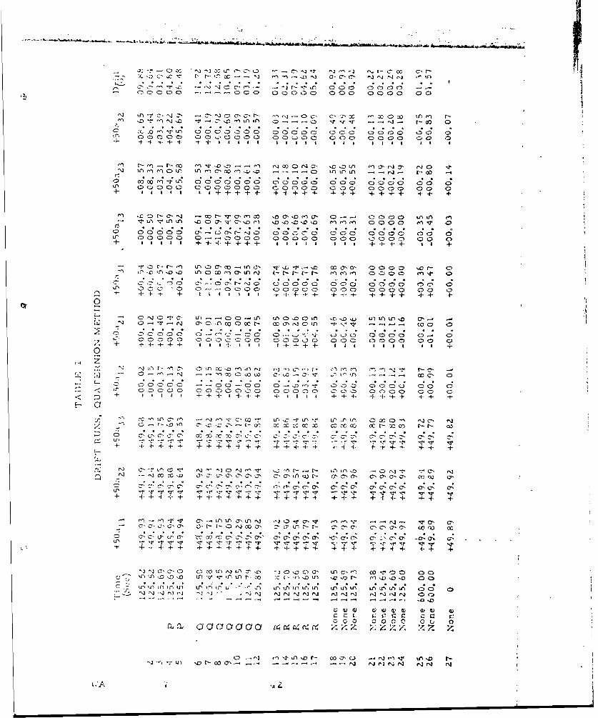
r-- 00'- ") OC'" jNif 000 0000Cl NII
-ý 0000CD0 -------- 00 0 000"D0 0 00 0 Q000 00C
Z, O- "tl f c'-,- -'r:-jr-c -- W x I t-o 0n r
o - U 0 000 00 0 0- )00 0000 c In f) (J 7 l 00m 00000 000 00 c'on 4) c c C) onLI -0
+4 4s #s e+*--+++ + -t++±-4- -4- +_+ . .-+++ + + +
fn .c 0'C'- -r- V'r0a'r) ~DO0O0 n l0 0--C' 000 atnf in I
0 0rýn 00 0 01 coo:o 000j0 C,0C -C, C D 0000 0 CD0 0+ + +a t ++ q+ +- +i i a i + +-?-4+ I
.0 *ror-D---D tfOIS'Io-1 0flC' (t'- I� r n i 00 000 mO 0". .rnn~ .f~r,'n~ .- 'N-,- .ff- 0.0 .a .0
::0C0 'DC C0 0-C, - r-NO C 0 000D0 0D0ý0 000C)0 CD0 00r 1:1 0ýIC) C ?C )r)Q 0--- 'o 0 000D 000 0 000 0 0 0+- + + + th+ £ 4--+- +--- f+ + + + + --
- -O O C- Lfl) ~ 0~f tflDOO 'NC)ýiC5a( C3.0L) Ln fw 0- U- ()0 N) C-1'r 1)0fco 0occr- cOD r'3'f il- C-.- cOO 0J r
L: rll: oC)o 0000000 C 000 0 00 000 ) )0 00 C+ + 4-++ - 4 +-il t+++ + lit bJl b +
- 0 000 -- 0-0 0.-D-fl 0 0 0 00 00 C_ 02C c-c P 0000 000 00 0000 C0 0 00 0 0
< D + b+il 4- + +t4_ + +ii -4+1 - ++- + + +
c'C ocýC, C,:' ,* -r 0 ci c',C: cC7 c-,s c-os c' 0 C'>c- C:+ 4-i4-++-t+ ++ ++. .-... 4- -- + 4- + + +- +-i---+ + + ±
-3 co) -r0,0 'D I.-C"0Nc C. C>0'fl'wnN (700 (__ -0--lC, - cr CQ a,
+ +-4+ 4- + + ++ +-4--4-+- -4- +-1- +-+ +I-f+ + + +
-' 13, -l --: -0, Q'-fhf IVr. -- 0:,n Q'c-N' t-l .r -j-- . 'r0 11'
- - 1' + -4 ~ 4- ±+ + + 4- + 4-+ ++4 4 +
In tlfIfliflhfL Ljr ' tf l'f Influ-t-'5 CC ~In Dt U-)n a-Ci f-a- CV)lULr 00D
In I) n- rx IF, In : I') U-%JNIn j NNN r-rs"J 00L)L nu) l l -
(JQw)4) (D))4 (D 4
00 00 00 0I
Jfl7) t~,0~ --- N r-rJN rj'Z fl
VA e AN
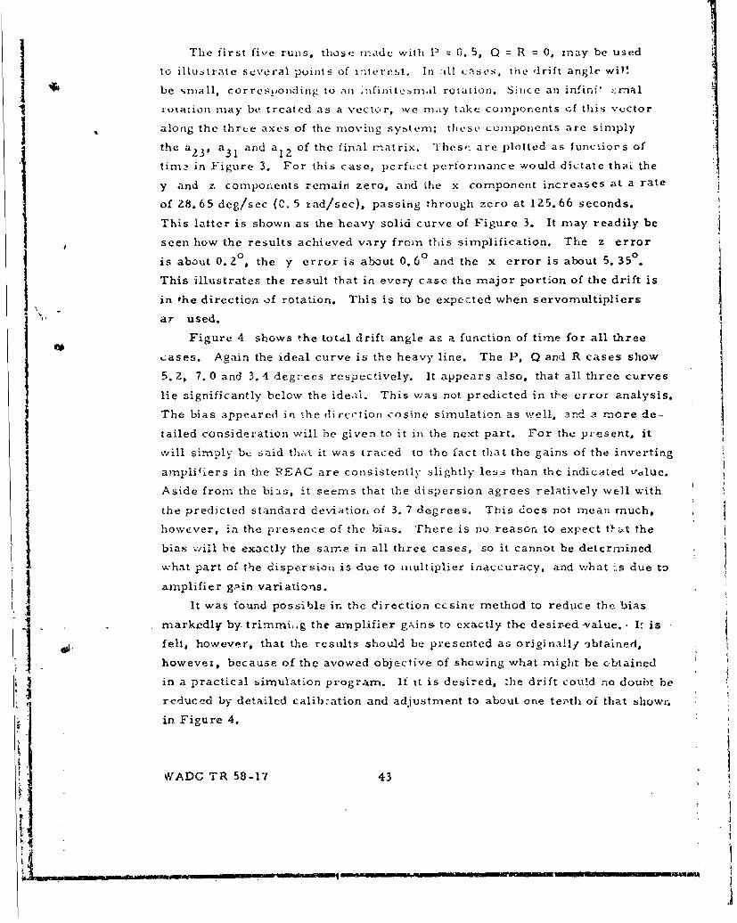
The first five runs, those made with P = 0. 5, Q = R = 0, mnay be used
to illustrate several points of interest. In :l1 c:ases, the drift angle will
be small, corresponding to an Mi iiittesnma1 rota!tion. Siuce an infini trnal
"rotation may be treated as a vector, we may take components cf this vector
along the three axes of the moving system; these components are simply
the a 2 3 , a 3 1 and a 1 2 of the final matrix. These are plotted as 1unc'ior's of
time in Figure 3. For this case, pcrfect performance would dictate thaL the
y and z components remain zero, and the x component increases at a rate
of 28.65 deg/sec (0. 5 xad/sec), passing through zero at 125.66 seconds.
This latter is shown as the heavy solid curve of Figure 3. It may readily be
seen how the results achieved vary frorn this simplification. The z error0 0is about 0. 2- the y error is about 0.,60 and the x error is about 5. 35.
This illustrates the result that in every case the major portion of the drift is
in the direction of rotation. This is to be expected when servornultipliers
"ar used.
Figure 4 shows the total drift angle as a function of time for all three
cases. Again the ideal curve is the heavy line. The P, Q and R cases show
5. 2, 7. 0 and 3. 4 degrees respectively. It appears also, that all three curves
lie significantly below the ideal. This was not predicted in the error analysis.
The bias appeared in the direction cosine simulation as well, a more de-
tailed consideration will be given to it in the next part. For the present, it
will simply bu baid that it was traced to the fact that the gains of the inverting
amplifiers in the REAG are consistently slightly less than the indicated value.
Aside from the bias, it seems that the dispersion agrees relati'hely well with
the predicted standard deviation of 3. 7 degrees. This does not mnean rnuch,
however, in the presence of the bias. There is no reason to expect tl-at the
bias will be exactly the same in all three cases, so it cannot be determined
what part of the dispcirsion is due to multiplier inaccuracy, and what -s due to
amplifier gpin variations.
SIt was found possible in the eirection ccsine method to reduce the bias
Smarkedly by- trimmi,ig the amplifier gains to exactly thb desired value. - I: is
, - -felt, however, that the results should be presented as originally" obtained,
however, because of the avowed objective of showing what might be obtained
in a practical simulation program. It it is desired, the drift could no doubt be
reduced by detailed calib:ation and adjustment to about one tenth oi that showln
in Figure 4.
WADO TR 58-17 43
t.a
S. . . It .. .-- - _ _7 -- | " ' "! . . . . -.. .. • 't
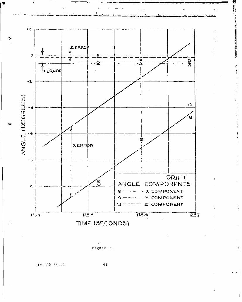
0d -4 L
I _ __
Li _ _ _- - _ _ _ _
_ _ _ _ _ _ _ _ _ _ __ _ _ _ _ _ _ _ _ _ _0
____-ANGL~E. COMPONENTSX 4CONAPONENT
~-----COMPONLNT
-I ME. (,5F.C.QND5)
kigurc.
*~; 1.I(L4{ ~44
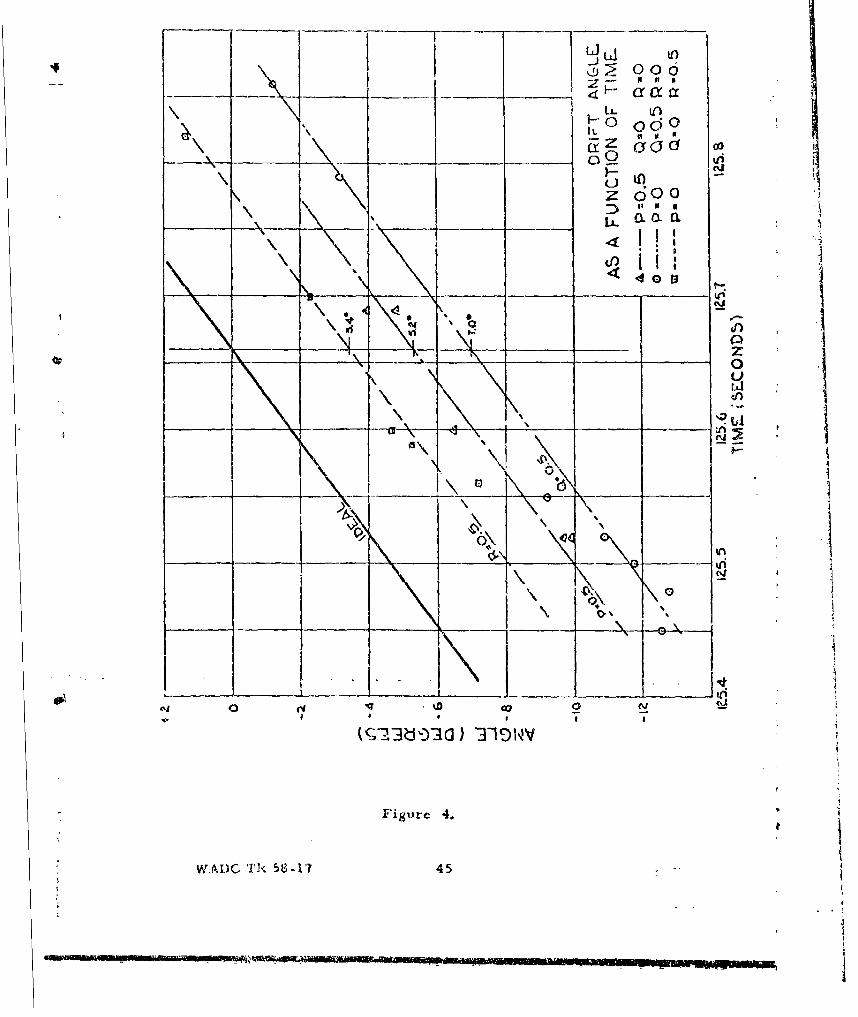
LJ t L
'9 0_ 000
4cLL~--- L I I if
0c0o\ z 6o00,
\ • I-LA .C -L Q- I N I
41K0\_•_ a'
'Ii
_ . _-. 0
X %,
Ui
aall
\ .1. o
I I\1 ,. U I U
Figure 4.
:W.AIC- 'T' 58-V? 45 .-
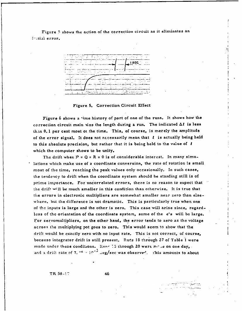
Figure _- shows the action of the correction circuit as it eliminates an
:tLial error.
Figure 5. Correction Circuit Effect
Figure 6 shows a lime history of part of one of the runs. It shows how the
correction circuit main -tins the length during a run. The indicated Al is less
than 0. 1 per cent most ot the time. This, of course, is merely the amplitude
of the error signal. It does not nccessarily mean that I is actually being held
to this absolute precision, but rather that it is being held to the value of I
which the computer shows to be unity.
The drift when P = Q = R = 0 is of considerable interest. In many simu-
lations which make use of a coordinate conversion, the rate of rotation is small
most of the time, reaching the peak values only occasionally. In such cases,
the tendency to drift when the coordinate system should be standing still is of
prime importance. For uncorrelated errors, there is no reason to expect that
the drift -4 11 be much smaller in this condition than otherwise. It is true that
The errors in electronic multipliers are somewhat smaller near zero than else-
where, but the difference is not dramatic. This is particularly true when one
of the inputs is large and the other is zero. This case will arise since, regard-
less of the orientation of the coordinate systern, some of the e's will be large.
For servomultipliers, on the other hand, the error tends to zero as the voltage
across the multiplying pot goes to zero. This would seem to show that the
drift would be exactly zero with no input rate. This is not correct, of course,
because integrator drift is still present. P.urs 18 through Z7 of Table 1 were
made under these conditLons. ron," 73 through -0 werc r-- -e on one day.
and a drift rate of 7. 'e ' r'- .ieg/sec was observe-. ,his amounts to about
TR 58 - 46
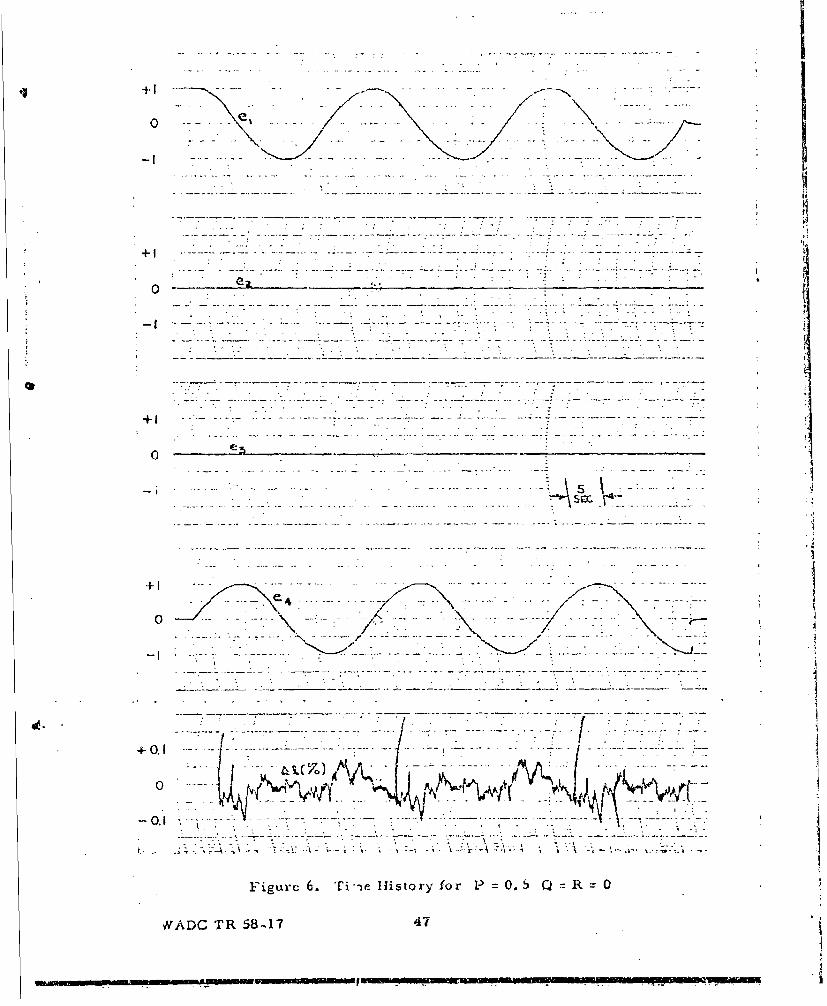
-7 - 7 -7 -- -
0-
-h~1 ........--. . -~~W
Figure .6. .T--ieH t..fo. 1.'=. 5 Q. R 0
NADC R 5817 4
e..

0. 0128 per cent of full scale (1 rad/sec). Runs 21 through 26 were made
abol-L a week after the preceeding set, after another problem had been on
t'e computer in the meantime. From this second set, a drift rate of about
2. 5 x 10- deg/sec was determined, an improvement by about the factor 3.
Integrators had been balanced in both cases, so the only conclusion possible
is that the zero-input drift is somewhat variable. It was found that the zero-
input drift was proportional to the maximum rate for which the computer is
scaled. The above results were taken for I rad/sec full scale, but some
runs were made with 5 rad/sec full scale, and the drift was almost exactly
five times as great.
While it does not appear utile to give the complete computer diagram,some remarks concerning the setup are in order. In order to accomplish thefunctions indicated in Figure 2, it was found necessary to use 36 summing
and inverting amplifiers, 4 integrators, and 8 multiplying serves, each with
three multiplying pots. On,.2 summing amplifier was used ahead of each inte-grator to do the summing. _ now appears that this was not wise, because
while the integrator gains proved quite accurate, the summing amplifier gains
were less so, and introduced an error in angular rate. The simulation wasnot found to be critical or sensitive in any way, except that the zero-input
drift varies somewhat from day to day. In all cases, however, it was q-=te
acceptable.
P. The Direction Cosine Method
The direction cosine simulation was done under as nearly the same conditionsas po.,sible. The same rate of rotation (0. 5 rad/sec) and th2 same full-scalerate were made and the same length of time was used. It was found necessaryto linme the runs with a Berkley counter, rather than the syncrhonous clock usedin the quaternion case because of the failure of the latter unit at the start of the
•.IC ~rurns. Such checks as could be made showed no significant differencein the timers. To do the operations of Figure 1, 31 inverting and summnng
.:.iplifiers, 6 integrators and 12 servomultipliers were required. Table 2 shows
the results obtained from reading the direction cosines at the end of each run.Again the rotation angle was plotted against time for each of the three inputs.These plots are given in Figure 7. Ag•¢n it appears that the three curves showsomething like the prv'diit-. di-- .ýsion, but a large bias also. The bias in this
58-17 48
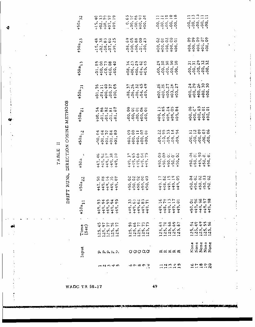
In r)tQ In- -0 0 -
C:' tnN cr- l 0C.0 000 000z 00,c: 00C )000itLf -0 0 C000 00CD C0)0 000 C cC D 0 C(D00
+ f f- -+-+4- -6 * + I 6
N ITc)c 0N 1 C)0cf0 CN] 0 0 v0 00 0N . . .. .
0 uý q cr-~ (70 -C)0 0 000( C)0 000.ý.- 00n 0n00 0000 0 00000r D )0n ýC
+ 66 6+6 + + +++ + +++ +
&) l) C) coo C) vr) 0, A <7*-D0000 C) C",N N
CI C5 .l .D N *clclc) f nr n
0D -000D0 c~o -0 'D '0000 0 00 0
+ 4 +6 + 4- + +4- 6 66 6
-l Ln ,-,o N Ln c, ~o ý r- .c r-
('3 . . . . . . . .
0nC -00Co0 c 0 0 0 0 C' 00000 00000
++ 4.+6+ 665 + + ++ ++ ++ +
N Itn 00 CO 0000 co 0 Q0~ 00 c a00
0 0- - 0000 0a aaC> 0 0000
+ +56 66+6 + +4 - ++++
ND 4 ýr"0 CT, CI- - - n le J
C' 0 0---- C 00C)000 C.)''O 000
U000 0000 0-000 0 000)
+ + 4++ + ++4- +6 6 +66666- 4-+
+ ++ +4--4 -- ++- + ++ +44 6 -+ +-+ +
++ .. + . ++ + - + ",4 1-4+ 4.+ ' v' + -r v
U -r'f~~f l ~ .Q -r -'D'D ,o Lr v ,f-u) '
0~ ~~~~~ 0~O a~-aoa 0~-ao ooo'o
N+q n 1 -0 +,4IN+M- +4+4+a4+4 4- ++ 1 0
WD TR. 581 49
""-mom~t6(f ~ 6~j~CL
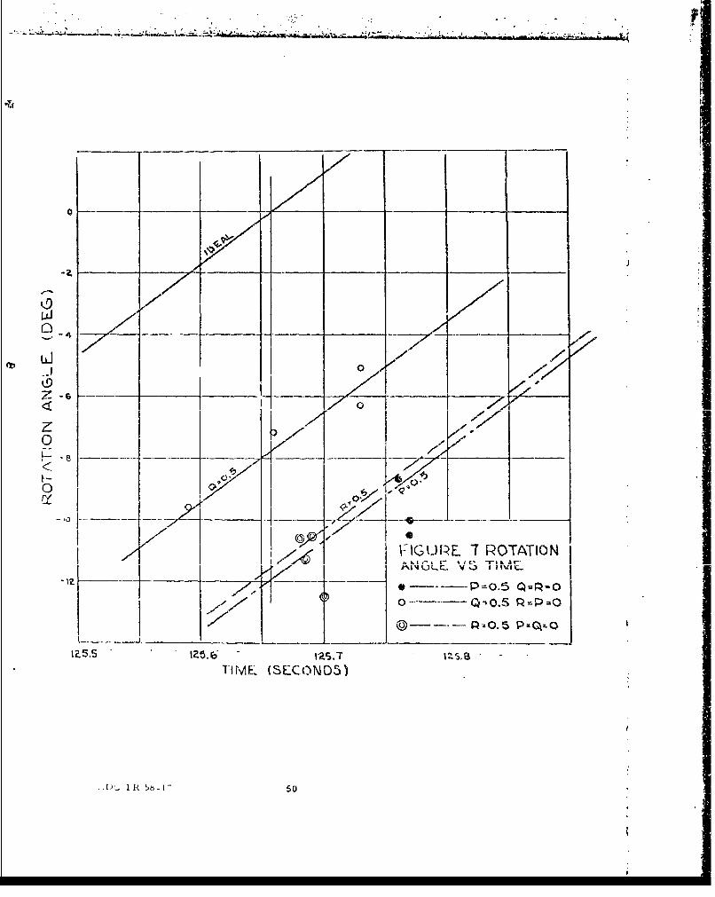
-1-
777
-xP-TK-A ((/'7N ci
050
case is nearly twice that found for the quaternions. The cause proved some-
what difficult to locate, and it is constructive to consider some of the checks
that were made in the process ef looking for it.
This bias amounts to an erroneous rate of rotation. The coordinate system
is rotating a trifle too slowly. In the example considered here, the system has
completed about 10 revolutions, turning through a total angle of nearly 3600
degrees. At the end of this time, it is in error by some 10 degrees or so. This
is one part of 360, surely not a large error, yet it is th'e predominant one, being
nearly three times as large as the error due to multiplier static errors. This
same bias, though smaller in size was observed in the quaternion simulation.
This leads to a strong suspicion that it is due to some characteristic of the
computing equipment itself, rather than some outright mistake in the setup.
To be sure, the setup was checked most carefully, many components were
interchanged and all the usual checking methods were applied with no result
other than to reaffirm that the equipment was correctly wired in accordance
both with the circuit diagram and the equations. Then checking of the counter
characteristics was started. It was thought that possibly the time base of the
computer (i. e. the time constant of the integrators) was not exactly the same
as that of the counter. To check this a linear 0. 5 rad/sec oscillator of 50 volt
amplitude was set up using only two integrators, two hand-set potentiometers
and one inverting amplifier. This oscillator was then allowed to run for 125. 66
seconds, and the result measured. The oscillator agreed precisely with the
timer. The output of the oscillator integrator which had a zero initial condition
(the other one had a 50 volt initial condition) went through zero within 10 milli-
seconds of 125.66, and the time error we are looking for is more in the nature
of 300 milliseconds. This is a surprisingly good check.
Next it was thought that it might be a phase lag effect. This was ruled out
by two experiments. First, a run was made so as to allow only five complete
rotations of the system rather than 10. It was found that the bias was very
nearly one half that of Figure 7. If it had been a phase lag effect, it would have
been more nearly constant with time. Furthermore,- the phase -lag-of a m-ulti-. -
plier was measured directly at this frequency, and was found to be about 0. 6
milliradians. The phase shift required to explain this bias would be more in
the order of 0. 1 radians.
By setting up a separate oscillator using two integrators and two servos,
the difficulty was finally traced to the fact that the summing and inverting
WADC TR 58-17 51
amplifier gains are consistently low. The gains were carefully adjusted in this
c_.,5,rate oscillator, and most of the bias was removed. It was not considered
orthwhile to similarly trim all the summers and inverters in the entire simu-
lation.
After all, the aim of this program was to show typical simulator results.
Still, if the ultimate accuracy of which the servos are capable is to be attained,
something of this nature should be done. It should be. mentioned that not all of
the amplifiers would have to be trimmed. Only those amplifiers which are
between the P, Q, and R multiplications and integrator inputs are critical.
None of those in the correction loops can give trouble. This is true of both
methods., It is rather surprising to find that servos, generally viewed with
suspicion and avoided when possible, should not prove to be the major source
of error in these simulations. Amplifiers, rather, have proved to be the
limiting factor.
It may also be showi from the data of Table Z, that the zero-input drift of
this method, at least on t. i day the runs were made, was about 3 x 10- 3 deg/sec.
This is comparable with the better set of results obtained with quaternions.
.R 58-47 52
SECTION VIII
SUMMARY AND UONCLUSIONS
Having investigated both quaternion and direction cosine coordinate
conversions, it is now in order to compare the strengths and weaknesses
of the two methods. For comparison purposes, the Euler angle method
will be included, though, as nientioned earlier, it is not str'ctly comparable
with the other two in capability. Before prQceeding with this comparisen, it
is well to outline the criteria. It seems that there a:c two main areas of
comparison. Listed in order of their importance they are (1) minimum
equipment requirement (both qualitative and quantitative) and (2) ease of
programming, reliability and comprehensibility.
As far as qualitative requirements on equipment is concerned, it has
been shown that both direction cosine and quaternion methods a: e equally
sensitive to multiplier errors. It further seems clear that since the Euler
angle system (as proposed by Howe and Gilbert)* makes use of the same
type of computing oscillator, it will be about the same as the other two in
this respect so long as the oricntation is well away frorm the singular point.
The dependence on error increascs as the singular point is approached,
however, until multiplier errors dominate the s:olution.
The fact that the multipliers oscillate only half as fast in the quaternion
method is of the first importance. There is no limit to the speed at which
the servos may be required to run in the Euler angle method, though Howe
and Gilbert* show surprisingly good results when servos are slewing.
It should be observed that the bandpass of even the rather old servos
used in this simulation is so good that it contributes nothing to the errors,
so long as thl sei5vos are operating linearly. The real problem in servos
is rate and acceleration limiting. it is on this point, then, that the lower
servo, frequency oa the quaterniQn method shows its real advantage.
*Howe and Gilbert, op. cit.
WADC TR 58-17 53
L a a
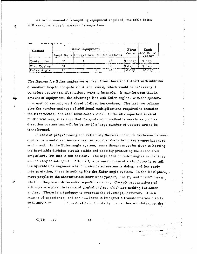
As to the amount of computing equipment required, the table below
will serve as a useful means of comparison.
Method Basic Equipment First Each7.Vector IAdditional
Amplifiers Integrators Multiplications VectorA t
Quaternion 36 4 26 9 indep 9 dep
Dir. Cosine 31 6 36 9 dep 9 depEuler Angle 16 6 .d.
The figures for Euler angles were taken from Howe and Gilbert with addition
of another loop to compute sin tI and cos ti, which would be necessary if
complete vector tra; sformations were to be made. It may be seen that in
amount of equipment, the advantage lies with Euler angles, with the quater-
nion method second, well ahead of direction cosines. The last two colums
give the number and type of additional multiplications required to transfer
the first vector, and each additional vector. In the all-important area of
multiplications, it is seen that the quaternion method is nearly as good as
direction cosines and will be better if a large number of vectors are to be
transformed.
In ease of programming and reliability there is not much to choose between
c.uaternions and direction cosines, except that the latter takes somewhat more
equipment. In the Euler angle system, some thought must be. given to keeping
the inevitable division circuit stable and possibly protecting the associated
amplifiers, but this is not serious. The high card of Euler angles is that they
are so easy to interpret. After all, a prime function of a simulator is to tefl
the orerator or engineer what the simulated system is doing, and for ready
interpretation, there is nothing like the Euler angle system. In the first place,
most people irk the aircraft.field know what "pitch", "roll"., and "bank" mean
whether they know differential equations or not. Cockpit presentations of
attitud.es are given in terms of gimbal angles, which are nothing but Euler
angles. There is a tendency to overrate the advantage, however. It is a
matter of experience, and on- -- , learn to interpret a transformation matrix
wit.. only a - .. • of effort. Similarly one can learn to interpret the
"ICT - 7 54
Finally, then, a simple statement of the coniIarJison is this: Euler
angles are convenient for interpiret ition, but for accu 'acy, they cannot icompete with cither direction cosines or quaternions. On all significant
bases of comparison, the qnaxterxiion mnethod appears superior to direction
cosines. Of course, it should be kept in mind that we are considering only
coordinate transfornmations capable of unrestricted rotation about any axis.
It might not be out of place at this point to interject a few remarks about
the general use of three-dimensional coordinate conversions of the type
considered here. It goes almost without saying, that such a coordinate
conversion would not be uscd except in a very large and involved simulation.
Another way of putting it is that in order to make this type of coordinate
conversion useful, other parts of the problem must receive a similarly
general and unrestricted treatment. This is very rarely done. The reason
is that the amount of labor involved is such as to be justifiable by only the
most overwhelming technical reasons. Computer capacity is not the limiting
Qk factor. ' here are many computer installations in the country whose capacity
is equal to the largest simulations yet attempted. The problem appears to lie
in the tremendous amount of painstaking detail involved to set up the problem,
check it out and keep it working. The only reasonable answer to this is a
policy of programming problerms in larger pieces. This is comparable to use
of subroutines on a digital inachine. Without going into the matter aL length,
it sccn-,s clder that coordinate conversion lends itself to this technique probably
better than any other part of the problem. Consider for excamnple, the quater-
nion method of Figure Z. The inputs to the coordinate conversion are the three
voltagcs P, Q, and R, and the outputs are the ninc direction cosines. There
are only twelve gains which would have to be changed from one prcblem to the
next, and these are the P, Q, and R product inputs to the four integrators.
These serve to establish the maximum allowable rate of rotation and the scale
factor on the inputs P, Q, and R. Nothing else in the entire circuit would have
tob ,,c .,,ang.d. Th,,e uni,-;.puter operator wvuuld nut even have to know how the
coordinate conversion worked. It would be converted into that "black box" of
which we are all so fond. By using this sort of technique throtughout the problem,
the amount of labor involved in large simulations could be cut by the factor ten.
This would simplify things other than the setup procedure. The engineer would
no longer have to spend so much time deciding what is negligible. He could
start everything in ani find what is negligible by throwing it out and seeing if
it changes the result, which, of course is in the best mathematical tradition.
WADC TR 58-17 55
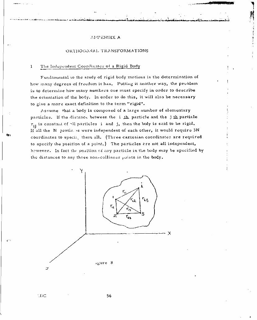
APPENDIX A
OR 1{THOQGOQNA L TRANSFORMATIONS
1 The Iridcpcndent Coordinates of a Rigid Body
Fundaniental to the study of rigid body motions is the determination of
how many degrees of freedom it has. Putting it another way, the problem
is to determine how many number:s one must specify in order to describe
the orientation of the body. In order to do this, it will also be necessary
to give a more exact definition to the term "rigid".
Assume that a body is composed of a large nmnber of elementary
particles. If the distance between the i .sh particle and the j 1h. particle
r.. is constait of -11 particles i and j, then the body is said to be rigid.
If all the N partic. ?s were independent of each other, it would require 3N
coordinates to speciy, them all. (Three cartesian coordinatez are required
to specify The position of a point.) The particles are not all independent,
however. In fact the- position cf azny particle in the body may be specified by
the distances to any three non-collinear j,&ints in the body.
'Y
S~rL
/-x
Atgure $
.7
".iC 56
The points !, 2 and 3 in Figure 8 havc been chosen at r-nnoom, the only
4 condiriLn bting th,,t they do not lie along the same line. By the rigid
body condition that ril I r.i2 and ri 3 are crnstant, the position of the i.tk
partichl is fixed once the positions of thls particle-s i, it follovs that the
position of every particle in the body is specified once: the three poinF are
specified. In other words, the position of the body is specified b- the positions
of these three points. Specifying three points would require nine coordinates
if all the points were independent.
There are three Londitions to be fulfilled by these coordinates, however,
namely the prescribed values of r 1 2 , r 1 3 and r 2 3Y Thus six coordinates are
required to specify the position of the rigid body. Another way oI saying this
is to say that the rigid body has six degrees of freedom. These are frequently
divided into two groups called translational and rotational degrees of fraedorn.
The three coordinates used to specify the orientation of some point in the body
(say the point 1 in Figure 8) In the xyz coordinate system, may be caled the
Stranslational coordinates, while the three ccordinates required to specify the
relative orientation of the other two points could be called the rotational
coordinates. The translational coordinates, then, are associated with the
motion of the body as a whole, while the rotational coordinates are associated
with the crientaton of te uC".
2. Orthnqrnal Tr;insforrnations
Consider a vector r which has components x, y and z in the XYZ
coordinate system. If the unit vectors along the X, Y and Z axes are
called i, j and k, then it is possible t,, write r as follows:
r = iX f j V + hza
Now assiune some .oordinate system X'Y'Z' which has the .same origin as
tile Z syszt ef Ou" an arbitrary x oation0 w"t"- r-espC-t to it. The coipo'.e-ts
of r in this system are x' y' arid z' and the unit vectors along the thr-eeaxes are V, j' arid k'. The vector 7 may ?lso bc written
r = i' x' + jy' + k'z'. (123)
The. problem is to determine thn components x', y' and z' in terms of xy and z
WADC TR 58.-17 ' 57
LII
and the relative orientation of the two coordinate systems. This process
is called an orthogonal transformation.
It is possible to write the unit vector iP in terms of its components in
the XYZ system,
i (i'Ji + (i'.j)j +(P. k)k. (12.4)
Since all these vectors have unit magnitude, the dot product of two is simply
the cosine of the angle between them.
Cos i = ali,
i*j= cos •il. = a12 , (15)
i'.k cos Li'•k = a 1 3.
The same process may be applied in obtaining j' and k'.
, (i,.t7+ + D. + Z.i )ki
so the entire set of relationships may be written:
7". -o- -4-a alii + a 1 2 j + a13 k,
= a2 1i + a,,j + aZ3 k, (126)
k'= a31i + a32i + a 3 3 .
It is possible to apply an exactly similar process in expressing the unit vectors
i, j and k in terms of their components in the X'Y'Z' system.
ai + a ' + a31
J = a 12 i- + a22j' + ak', (127)1 . - 3
k = a 1 3 i' + a 2 3j' + a33k'
Figure 9 shows the two coordinate sy.3tcms and the unit vectors.
..A 58-l7 58
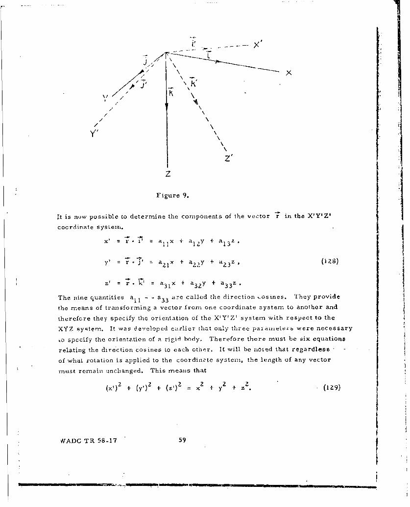
J r 1 1'/ \
/\
/k/\7'.
Z'
Figure 9. i i
It is now possible to determine the components of the vector r• in the X'y'z'
= . = a1 lx + a1Y+ a .7.
z' r.' a31x + a 3 2 Y + 33z.
The nine quantities a - - a 3 3 are called the direction ,-osines. They providethe means of tranisforming a vector from one coordinate system to another and
therefore they specify the orientation of the X'Y'Z' system with respect to the
XYZ syvtem. it was developed earlicr that only three paratlictevrb were necessary
ko spccify the orientation of a rigid body, Therefore there must be six equations
relating the direction cosinesto each other. It will be noted that regardless
of what rotation is applied to the coordinate system, the length of any vector
must remain unchanged. This means that
2 2 2 2 2 2xT )+ (y,59 + x 4 y z.
SvWADC TR 58-17 59
Substitution of the Equations (128) into this equation sho-ws that if Equation
"." is to hold identically for all values of x, y and z, then the following
, 1:ditions must obtain:
2 2 z
aI + a 2 1 + a31 =
2 2 za12 +a 2 2 + a32 = 1
2 a22 2 1
a 1 3 +a 2 3 + a33 - 1(130)
a 11al2 +- a21a2Z I a 31'32 -- 0
+a a 2 ++a a t = 0,a11a13 + a21a23 ÷a 3 1a 3 3 - 0,
a12a13 + a22 a23 + a32 a33 -0
These six equations are ,.lied the orthogonality conditions. The entire set of
equations may be written in condensed form as
aija.ik = 6 jk (131)
i
where 6 jk s the Kronecker 6-symbol which is defined by
S.k 1. (j k)(132)
6. 0 k).
It will be noted that the nine direction cosines, restrained by the six orthogon-
ality equations give the three independent parameters necessary to define the
oricitatio,' of a rigid body. The nine direction cosines may be written in an
array called a matrix.
a1 a12 a13
a: a 3 -- (A). (133)
S32 a3 3
'R 58-17 60
Matrices are a type of mathematical entity which may be conveniently
applied to the problem of rigid body rotations. The rules for manipulating
these quantities will now be reviewed.
3. Properties of Matrices
The multiplication of a matrix by a vector is the first operation of
interest. Symbolically, this is represented by
(A = (A)r. (134)
For convenience, the x, y and z components of r are denoted by xI xz and
xy Note that a vector r may be viewed as a matrix of only one column.
The equation might be written
a3 22a a~~(j (135)
Sx2 -- 21 a22 a23) x 15,x3' •31 a32 a33 x3,
The rule for performing this operation is
3.
x1 a~ .x. . (136).j-
If these operations are carried out, a set of three equations is obtained which
is identical with the set of Equations (128). This means that multiplication of
a vector by matrix using the multiplication rule above represents a transfor-
mation of that vector from one coordinate system to another. For this reason,
the matrix (A) may be called the transformation matrix.
The case of two successive rotations is an important one. Let the first
rotation-be-represented by a. matrix (.B).- T-hen the oorrponents of a-vector
after this rotation will be given by
b= k bjx. j (137)
WADC TR 58-17 61
• I. I l II I l I I
If the secorid rotation is vepresented by the matrix (A), then t1! components
of the vector after this second rotation would be
•"' =7_ "ikk ('skI,
Substituting (137) into (138) gives
ai Lik bkX.
k j
Sj k
Note that this can be ?ut in the form o; Equation 136.
x'' = c..x. , (139)
j
wherec.. = I-2- akbk. (140)
k
Thus the two rotations may be replaced by a single rotation (C), the elements
of which may be computed from (140). Symbolically,
(C) = (A) (B). (141)
It can be seen by the rule of Equaticn (140) that
(A) (B) it 'B) (A•)
so the procesp of matrix multiplication is not ccmmnutative. The process of
rnmatrix multiplication is associative.
(A) [(P.) (C) ] = [(A•) (B)] ( )
The ,matrix (A) was used to transforin tho vector r into the vector r'.
It is of interest now to investigate the properties of the matrix (A)-
which trancfornim i. ;o r. The clements of this inverse matrix are desig-
;i . 'hev inverse niatrix is dcfined by the following eq::ation.
(A) (A) r r. (14z)
WVADC Tit :6-1i6
Doing the first operation, the result is
a-' > a..x.. (143)
Now applying the inver.sc transformation to this gives
x a a X .Xk' k. i '
i 3
xk 3kajxj,j4J-i j
Now according to the requirement that this must give baclk the original vector,
xk' > cc. This will be true only if
7 ai a.- (144)Z- • 6jk
11
This shows that the product of the two rnatrices (A) and 'A)- will be
(A)" 1 (A) = 1 0 = (1) (145)
0 0 1
This matrix (L) is called the identity naatrix. It mna,, oc easily shown from the
rules of matrix multiplication that far any matrix (Q),
(I) (Q) = (a) (1) = (0) (i46)
Now sinc-e (A-)- corresponds-to some phy-ical rotation; there must exist some
matrix (K) which it, -he inverse of (A)-. ]n other words, there rm.st be an
(R) such that
(n) (A)- (M). (147)
How if (R) is appL: ed to both sides of Equation (145), ths result is
(R) (A)" (A) (R) (I) = (R). ( 18)
WADG TR 58-17 63
i !. . .
Si.nce matrix multiplication is associative, Equat .on (147) may be substitited
into Equation (148) to give
(1) (A) - CR)(A) - (R)
This means that
(A) (A) (A) (A) = (I), (L49)
so that (A) and (A)- commute.
Now consider the double sum,
j aijak1aI aki . (150)
k,i
This sum may be written two ways, depending on the order of summation,
k I i i kJ
Applying Equation (144) to the quantity in parentheses on the left hand side,
and applying the orthogonality condition of Equation (1 31) to the quantity in
parentheses on the right hand side, the result is
6 6 Jk akl1 6 I a.., (152)k
a-' a= a
This is the important result. To form the inverse of an orthogonal matrix,
the rows and columns are simply interchanged. Note that this conclusion
holds true only for orthogonal matrices. This is because the orthogonality
conditions were used to prove Equation (152). in general, the matrix formed
by interchanging rows and columns is called the transposed matrix and is desig-
nated by (A). The complex conjugate of this transposed matrix is called the
adjoint matrix and is indicated by (A)+ (A) A matrix is said to be unitary
if it satisfies the condition,
(A)+ (A) = (1). (153)
Of course ti., -c 1,:, definitions are relatively meaningless in the case of
re~al ,•--""s. However, use is sometimes made of matrices, the elements
iare complex numbers.
WADC TR 58-17 64
It is of interest to investigate the charactf-rislics of the determinant
formed by the element of a matrix. T ic determinaint of the matrix (A)
will be written as [A]. It will be noted that the law of matrix .nailtiplication
is the same as the law for multiplication of determinants. Therefore,
[AB] [A] [B]. (154)
Evidently the determinant of the identity matrix has the value unity,
therefore, from Equation (145) it xnay be seen that
A.-1] [A] = 1. (155)
provided that (A) is orthogonal. Since interchanging rows and columns does
not alter the value of a determinant, [.A-'] = [A] and, from Equation (155),
[A] 1. (156)
This means that the determinant of the transformation matrix can have only
the values plus or minus one. If the rotation is a real one, it may be shown
that +1 is the only allowable valae. There is a certain type of matriL opera-
tion which is called a similarity transformation. It is defined by
(A)' (B) (A) (B)1. (157)
Jt can easily be shown that the determinant of (A) is the same as the determinant
of (A)', that is to say, the value of the determinant of a matrix is invariant undi-r
a similarity transformation of that matrix. This may be shown by simply apply-
ing both sides of (157) to the matrix (B).
(A)' (B) = (B) (A) (B)- (B) = (B) (A). (158)
From this it is seen that
[A'] [B] [B] [A]. (159)
d Since [B] is a number and not zero, it is possible to divide both sides by it
and obtain the result
[A]= [A'], (160)
which demonstrates the propo,;ition.
WADG TR 58-17 65
~~ , -
There is another set of relationships among the direci..on cosines which
will prove to be of interest. Consider the set of Equation.; (IZ6). If the
i', j' and k' vectors are mutually perpendicular, then t.',e following relation-
ships apply:
i' x j' = k', ' x k' = , k' x i = . (161)
If these vector equations are expanded in the unprimed system, and their
components equated, the result is
a11 -a 2 2a 3 3 "a2 3 a 3 2 1
a21 a a -a a
a1 a a -a aSa31 = 12a23-a13a22,
a -a 2 a3 1 a a!2 23 az31-a11 23
a 2 2 11 a 33-a13a31 (162)
a 3 2 -a 1 3a 2 1 -a1 1 23
a13 - a2 la 3 2 -a2 2 a 3 1 ,
a23 a 12 a31-a 11a32
a 33 -ail,,,-al2a.1-
These nine equations are really consequences of the orthogonality conditions.
They present a means for solving for any direction cosine in terms of the others.
4. Infinitesmal Rotations
It wou.d be great advantag• if a vector cnuld be associated with a finite
rotation, but it turns out that this is not possible. For-one thing, finite rotations- ...
are not commutative, nor even anti-commutative. That is to say the order of
the operations must be preserved. While this is true of a finite rotation, it will
be shown that a vector may be associated with an infinitesmal rotation and that
therefore, the known characteristics of vectors may be used in the treatment of
such rotations. Cosi(icl:r the matrix that describes a rotation thru the angle
1' •hich makes the angles a,, P1 and y1 with the X, Y and Z
'v,.J-. DC TR 58 -17 66
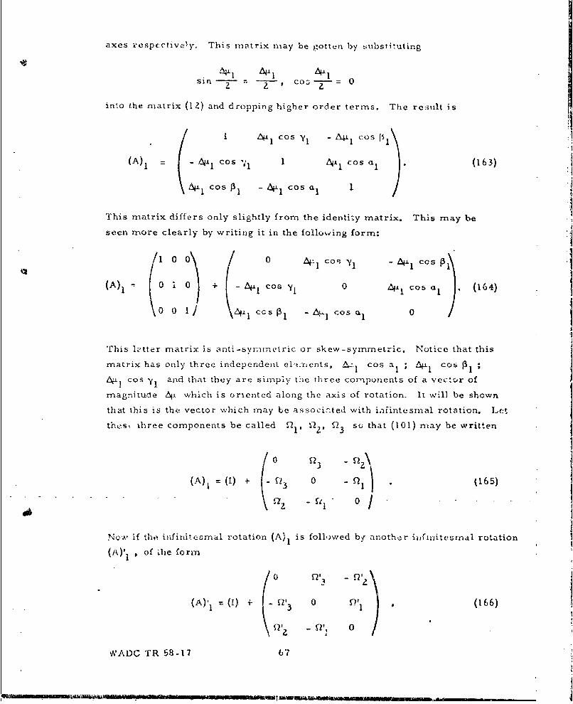
axes respcctivelyo This matrix may be gotten by substituting
sin-- = t 1--- co 11Z 0
into the matrix (12) and dropping higher order terms. The result is
/ ' ±1 cos Y1 -A41I Cos fil
(A) 1 (-4•lcos 1 0t cos al . (163)
Ai cos •I -4i.1 cos a 1
This matrix differs only slightly from the identi'y matrix. This may be
seen nmore clearly by writing it in the follow~ing form:
/ 0 / 0 4- 1 Cof Y -- Al ICoso P
(A), 0 0 + -jlCoY,0 NlCos a, (164)
A~1 cs~1 ~ Cos a. 0
This lhtter matrix is anti-symmetric or skew-symmetric. Notice that this
matrix has only three independent el.'nments, Cos al ; 6'L cos P,64x1 cos y3. and that they are siimply the three cornponents of a vec-or of
magnitune 64- which is oriented along the axis of rotation- It will be shown
that this is the vector which may be associ.-.ted with iafintesinal rotation. Let
thst three components be called O2 12 Q 3 su that (101) may be written
(A) (1) + o 0 Qv .(165)
Now' if thte infinitesmal rotation (A) 1 is followed by, another infinitcsrnal rotation
(A)' 1 , of dlie form
\Q, z -J 1 01
W'ADC TR 58-17 67
I:T W'. I MW W M
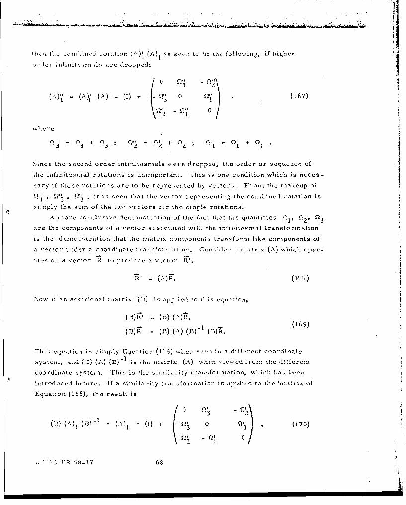
¾ ~ . .. ' .. .. ' 4 .... . ... .. .
lilt n te coinbi ned roiatiin (A)' (A) s seen to be the following, if higher
rdel i:ifinlit s 1 arv droppdcd
(:") = (A); (A) + "' 0 M (167)
where
= : ý + f3; !,' =S$+ Q? + Q2 •
Since the second order infinitesrnals were dropped, the order or sequence of
the infinitesmal rotations is unirnportant. This is one condition which is neces-
sary if these rotations are to be represented by vectors. From the makeup of
', . , ý2'ý 0 it is seen that the vector representing the combined rotation is
simply the sum of the Iw, vectors tor the single rotations.
A more conclusive demonstration of the fact that the quantities Q 1 , •QZ Q
are the components of a Vector associated with the infifitesmal transformation
is the demonutration that the matrix components transform like components of
a vector under a coordinate transfor-naline., Consid-r ;i matrix (A) which oper-
cites on a vector R to produce a vector R'.
' = (A,^)4 . (168)
Now if an additional x,,atrix (B) is applied to this equation,
-l (169)(1)R, : (n) (A) (B)- (')aR.
This equation is siniply Eqvation (168) when seen in a different coordinateby tcnz, anCd IA, In) i '4 -.. icd fr".. t:• the different
coordinate systemn. This is the similarity transformation, which has been
introduced before. If a similarity transformation is applied to the 'matrix of
Equation (165), the result is
0 n0S1
(B) ('A) (13 1 -)_ (..' 1 = (1) ( 0 jcsl (170)
L. T'k 58-17 68
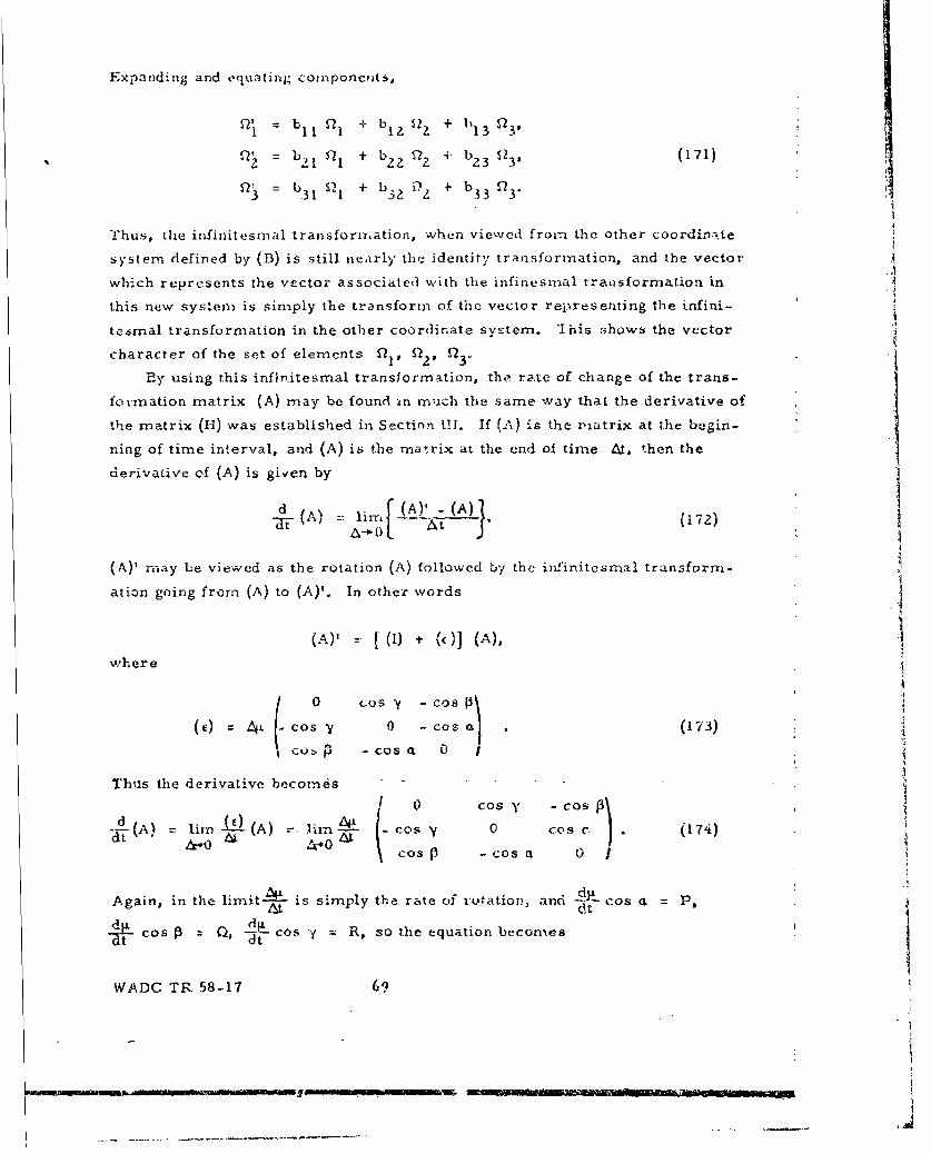
Expanding and equating components,
11',] b1 1 1- + blz S2z + 1)13 23P
f£2 = bu Q1 + b22 Q2 bZ3 S239 (171)
Q2 + 4b + 4b Q2=31 1 + b z 33 3'
Thus, the infinitesmal transformation, when viewed from the other coordinate
system defined by (B) is still nearly the identity transformation, and the vector jwhich represents the vector associated with the infinesmal transformation in
this new system is simply the transform of the vector representing the infini-
textmal transformation in the other coordinate system. 'Ihis shows the vector
character of the set of elements 2l. Q23 !43*
By using this infin.itesmal transformation, the rate of change of the trans-
fotmation matrix (A) may be found in nmach the same way that the derivative of
the matrix (H) was established in Section 111. If (A) is the nmatrix at the begin-ning of time interval, and (A) is the matrix at the end of time At, then thederivative of (A) is given by
d [SA)' - (A)t)
-( F ( A ) Z -- 1o T .n - ( 1 7 2 )
(A)' may be viewed as the rotation (A) followed by the infinitcsmal transform-
ation going frorn (A) to (A)'. In other words
(A)' [(I) + G )] (A),
where
0 co-SY - Cos~
(C) - Cos y 0 -Cosa , (173)Scozi P cQ3 a 0 !"
Thus the derivative becomes )I 0 cosy -Cos
=at A urn (A) - lIrnA -Cos v 0 Cos C. (174)
Again, in the limit-- is simply the rate of r'outatiorn, and d'- cos a =1
At CAitCsa P
.Cos d 0, t cos f = R, so the equation becomesdt dt
WADC TB. 58-17 69
Uv~aa~sN~aunrnfflf~ sa wsa~nin inu
j
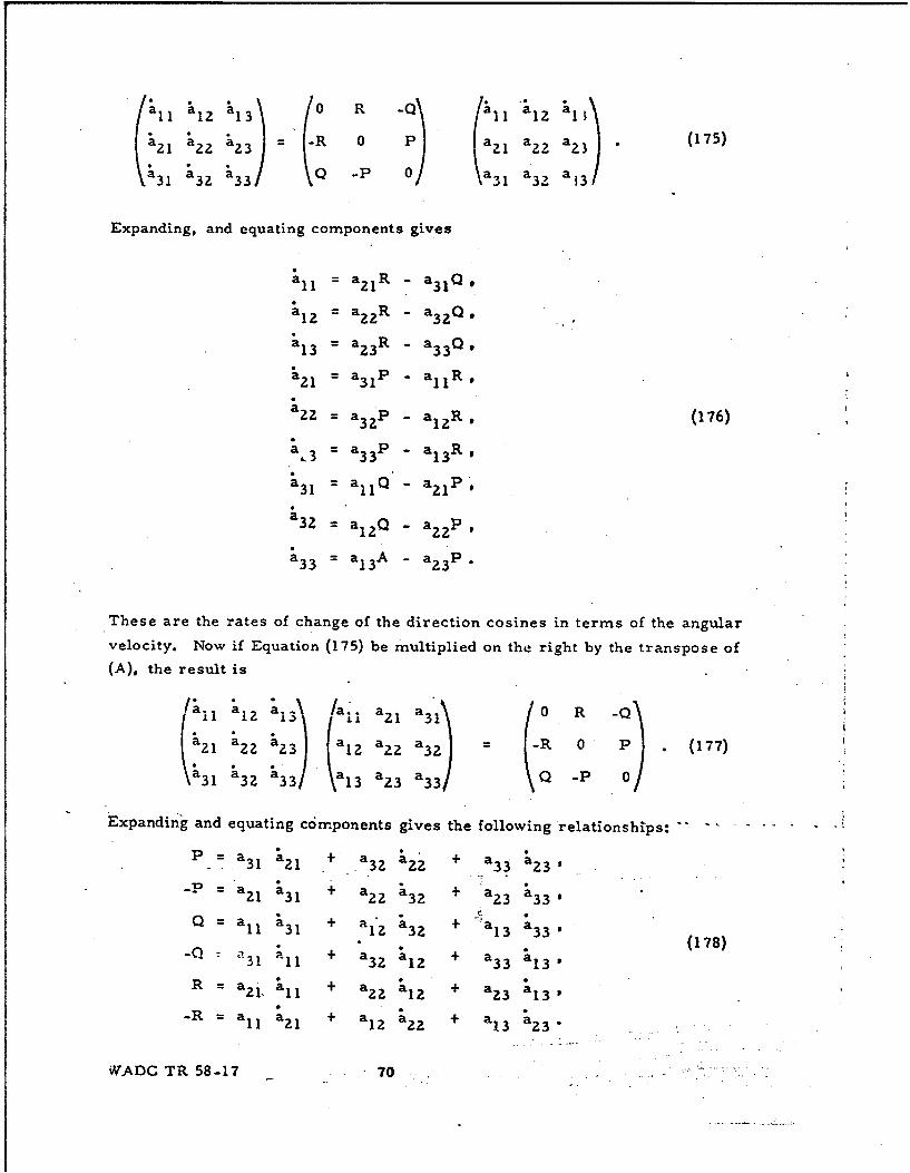
(a ll a3 / 0 R -Q\ all a,,2a
ý21 ý22 4:) -R 0K::: a., a 23(175)31 32 33) a 3 2 aB
Expanding, and equating components gives
a11 = a 2 IR -a
a -a 2 2 R -a
13 a 3R -33
a1 -a 3 1P "a- R
a2Z = a p 2R (176)
a.3 = '33 P - a13R'
a31 - a1 1 Q' - a2 1 P ,
a32 = al 2 Q - a22P
33 = al3A - a2 3 P.
These are the rates of change of the direction cosines in terms of the angularvelocity. Now if Equation (175) be multiplied on the right by the transpose of(A). the result is
1 1 2 1 aLaz a310 R -
2~1 ý22 23 2 z 22 a 32- = (177)
31 a&3 a33) a13 a23 a33) -P 0
Expanding and equating components gives the following relationships:
P 3 1 21 + 23z2 + 33 a2 3 '-P31 + a a + a
S 31 22 32 Z 33a=a1 31 + a12 a32 + •a13 '
• 3a 3 (178)-Q a3 1 a 1 1 + a32 3 a12 + a33 a.1 3 .
R = a2 1. I'11 + a 2 2 a1 2 + a23 a1 3,-R = a a21 + a12 22 + a1 3 a 2 3 "
WtADC TR 58-17 70

It is interesting that two different expressions are obtained for each of the
velocity components. This is a consecucnce of the great amoulnt of redundancy
in the direction cosines. The equivalence of the two expressions for any one of
the components may be shown by making use of Equation (162).
WADC TR 58-17 71
APPENDIX B
THE EULER ANGLES
It was demonstrated in Appendix A that three parameters were required
to fix the orientation of a rigid body and hence of a coordinate system. The ninedirection cosines do not lend themselves to a reduction to three simple para-
meters, nor do they give a very lively picture of the orientation of the body.
Both these difficulties are overcome by use of Euler angles, the only three-para-
meter system in common use. In this method, a rotation is represented by threeindividual, rotations taken in a specified sequence about certain specific axes. In
the literature, there is no agreement whatever on the order of rotations, the axes
about which the rotations are made, or notation. These are varied to suit the
needs of the problem and/or the author's whim. Texts on classical mechanicsgive sets of angles defined so as to facilitate solution of the spinning top problem.
The system presented here is the mnst common, though by no means the only one
used 3n aircraft work.
Consider two coordinate systems initially coincident. One set of coordinates,the x, y, z, will be referred to as the fixed system, and the other will move with
respect to it. The first rotation is through the angle 4 about the z' axis. This
is shown in Figure 10.
WADC TR 58-17 72 '
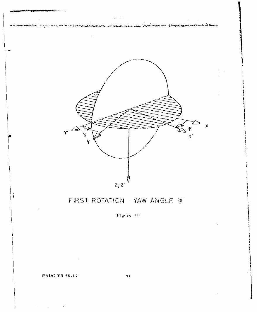
2' Z'
FIRST ROTATION vY,, PA W A' ANGL F
Figure 10
WADC TR 58-17 73
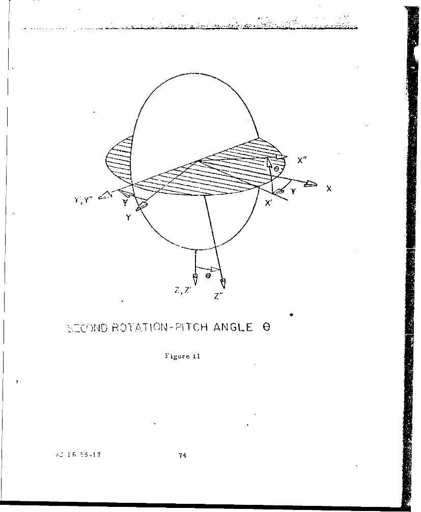
~.iT tD -K~TIONIrPITCH ANGLE 0
F~igure 11I
). ... . ...-° 74
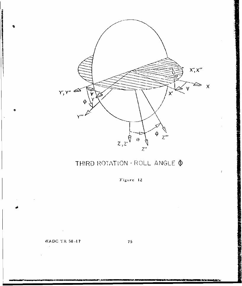
Yo y"f
THIRD ROTATION - FROLL ANGLE q)
Figure 1
ivVADG TR 58-17 75
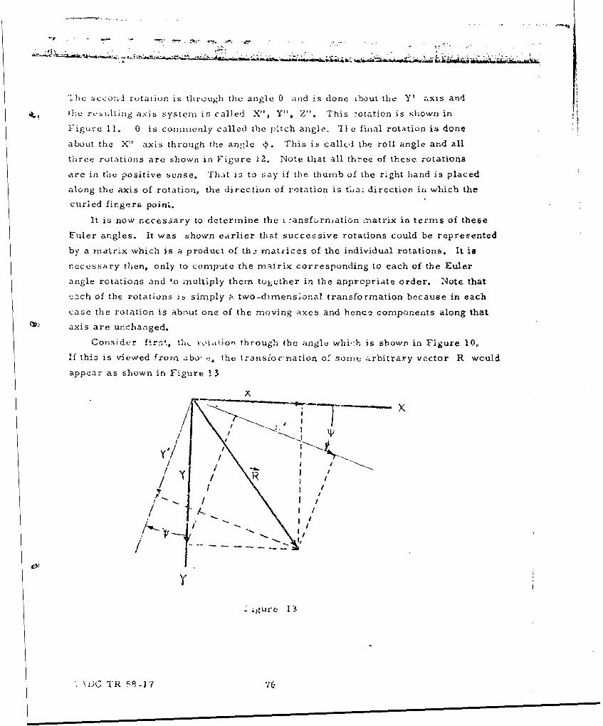
* • • . , -... . . -- j . ' .. . ... - . . . .
"1The sccond rotation is through the angle 0 and is done lbout the Y' axis and
It2he rebulting axis system is called X"' Y", Z". This rotation is shown in it
Figure 11. 0 is coninionly called the pitch angle. 'lIe final rotation is done
about the X" axis through the angle ,.. This is callcd the roll angle and all
three rotations are shown in Figure 12. Note that all three of these rotations
are in the positive sense, That is to say if the thumvb of the right hand is placed
along the axis of rotation, the directiun of rotation is t?,aL direction in which the
curled fingers point.
It is now nccessary to determine the v :ansfurniation matrix in terms of these
Euler angles. It was shown earlier that successive rotations could be represented
by a matrix which is a product of th.. matrices of the individual rotations. It is
necessary then, only to compute the matrix corresponding to each of the Euler
angle rotations and .o multiply them together in the appropriate order. Note that
inch of the rotations is5 simply a two-dimensionai transformation because in each
case the rotation is about one of the moving axes and hence components along that
axis are unchanged.
Consider firs°. thL t-,tnrion through the angl, which is shown in Figure 10,If this is viewed from abo-, o the transior-nation of soint arbitrary vector R would
appear as shown in Figure 13
x
/-) xI i
, j
t/ /
O://
-. ±gui'c 153
"V \P)C TR E8-17 76
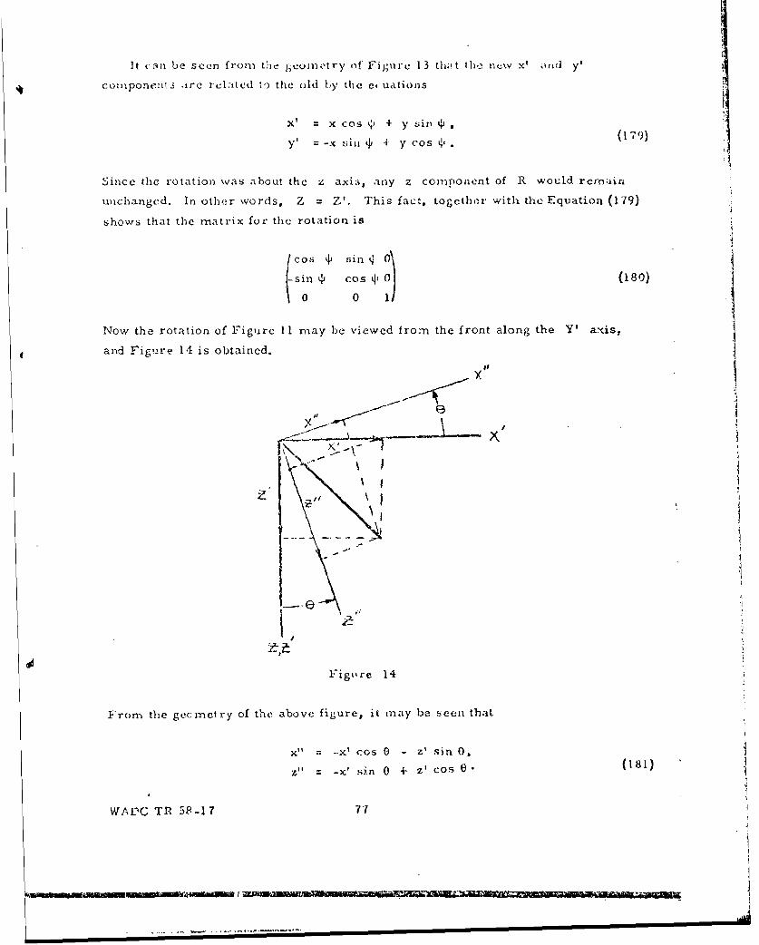
It c an be seen frorn the geoiný try of 1--iguir. 13 thi t the new x' old y'
comnponento ,ire rclited t,) the old b y t01e e uations
x' = x cos 4' + y sill ,( 9
y, =-x ziii 4. y cos (179)
Since the rotation was about the z axii, any z component of R would remanin
unchanged. In other words, Z = Z', This fact, togethar with the Equation (179)
shows that the matrix for the rotation is
fcos ' sin4 o\-sin o' cos 4'0 (180)
00 ii
Now the rotation of Figure 11 may be viewed from the front along the Y' axis,
and Figure 14 is obtained.
'I#
i e x
' I
Figure 14
From the gecmetry of the above figure, it may be seen that
X" = --x' Cos 0 2' sin ,
= -x' sin 0 4- 2' cos e- (181)
WAPD TR 5P-17 77
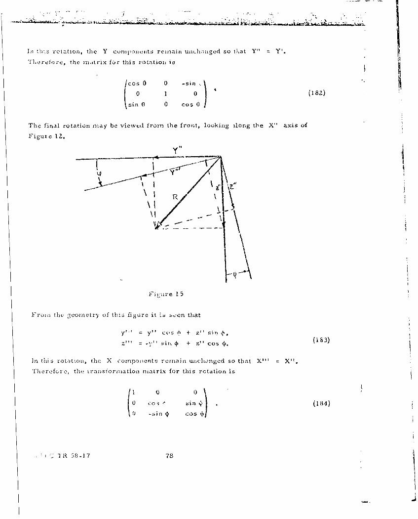
In this rotation, the Y comp.ml: nts remiain unuhaiingcd so ifat Y"' Y'.
'1"'eret(rc, the matrix fur this rotation is
Cos 0 0 -sin/ { 0 1 0/ •-sin 0 0 Cos 0
The final rotation may be viewed irorn the frort, looking ilong the X" axis ofSFigul e I Z.
Fit,1ure 125
SFromn the geometry of this figure it izi bocn, that
-y'' = y" cos c - z" sinZ'" = -•"•I ý + 7", Cos .(183)
)In this rotation, the X components, remain unchanged so that X.. X".''lcflrc the r ornthe ransformation mair rix for this rctation is
c b,(184)
I - R 58 -17 78
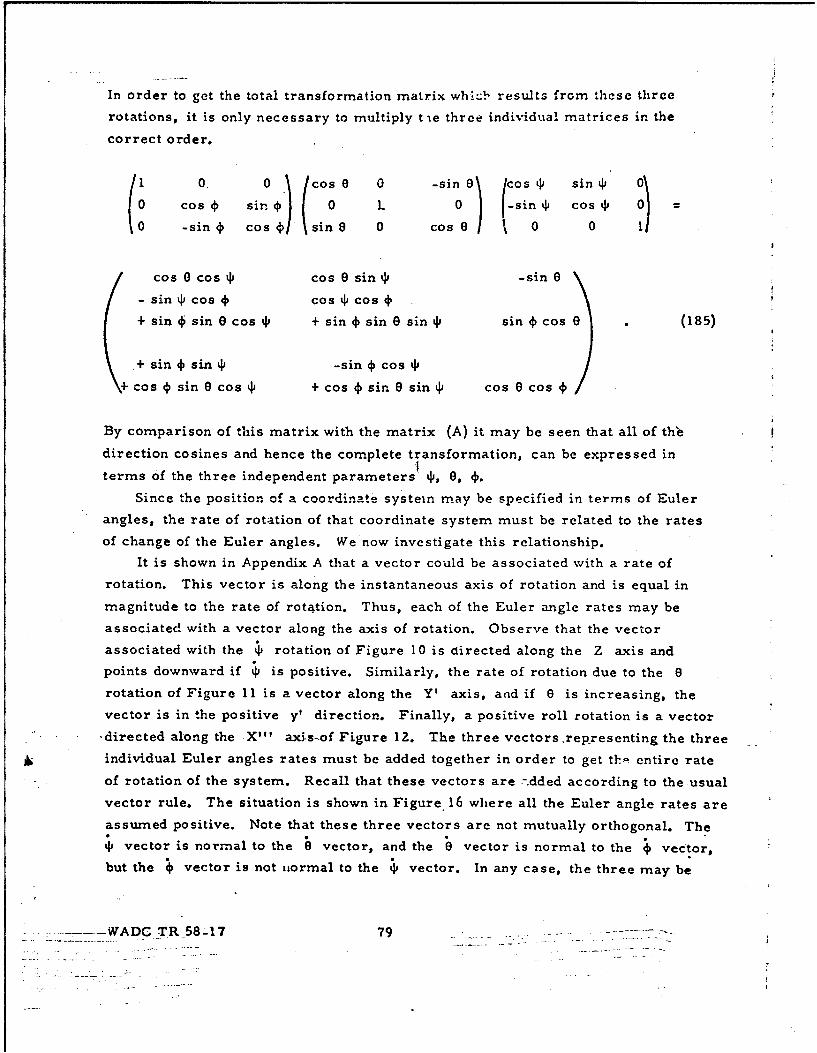
In order to get the total transformation matrix whý:.!- results from dhesc three
rotations, it is only necessary to multiply tie three individual matrices in the
correct order.
1 0. 0 cos0 0 -sino a cosiP sino 0
Cos os sin 0 L 0 -sin Cos =
-sin 4 si sin 0 0 Cos 0 0 0cs
cos 0 cos J cos 0 sin 4 -sin 9
- sin 1P cos4, cos 'cos4,
+ sin 4sin 0 cos ip + sin + sin 0 sin 41 sin ý cos0 (185)
+ sin •sin ij -sin 4 cos 1P
+cos 4, sin 0 cos J + cos 0 sin 0 sin cos 0 cos 40
By comparison of this matrix with the matrix (A) it may be seen that all of the
direction cosines and hence the complete transformation, can be expressed in
terms of the three independent parameters f, 6, ',.
Since the position of a coordinate systein may be specified in terms of Euler
angles, the rate of rotation of that coordinate system must be related to the rates
of change of the Euler angles. We now investigate this relationship.
It is shown in Appendix A that a vector could be associated with a rate of
rotation. This vector is along the instantaneous axis of rotation and is equal in
magnitude to the rate of rotation. Thus, each of the Euler angle rates may be
associated with a vector along the axis of rotation. Observe that the vector
associated with the 4 rotation of Figure 10 is directed along the Z axis and
points downward if 4 is positive. Similarly, the rate of rotation due to the 0
rotation of Figure 11 is a vector along the Y' axis, and if 0 is increasing, the
vector is in the positive y' direction. Finally, a positive roll rotation is a vector
-directed along the X111 axis-of Figure 1Z. The three vectors.representing the three
individual Euler angles rates must be added together in order to get thp. entire rate
of rotation of the system. Recall that these vectors are .-dded according to the usual
vector rule. The situation is shown in Figure. 16 where all the Euler angle rates are
assumed positive. Note that these three vectors are not mutually orthogonal. The
Svector is normal to the b vector, and the b vector is normal to the ; vector,
but the • vector is not normal to the i vector. In any case, the three may be
---.---- WADC TR 58-17 79 ._-* .--..... .
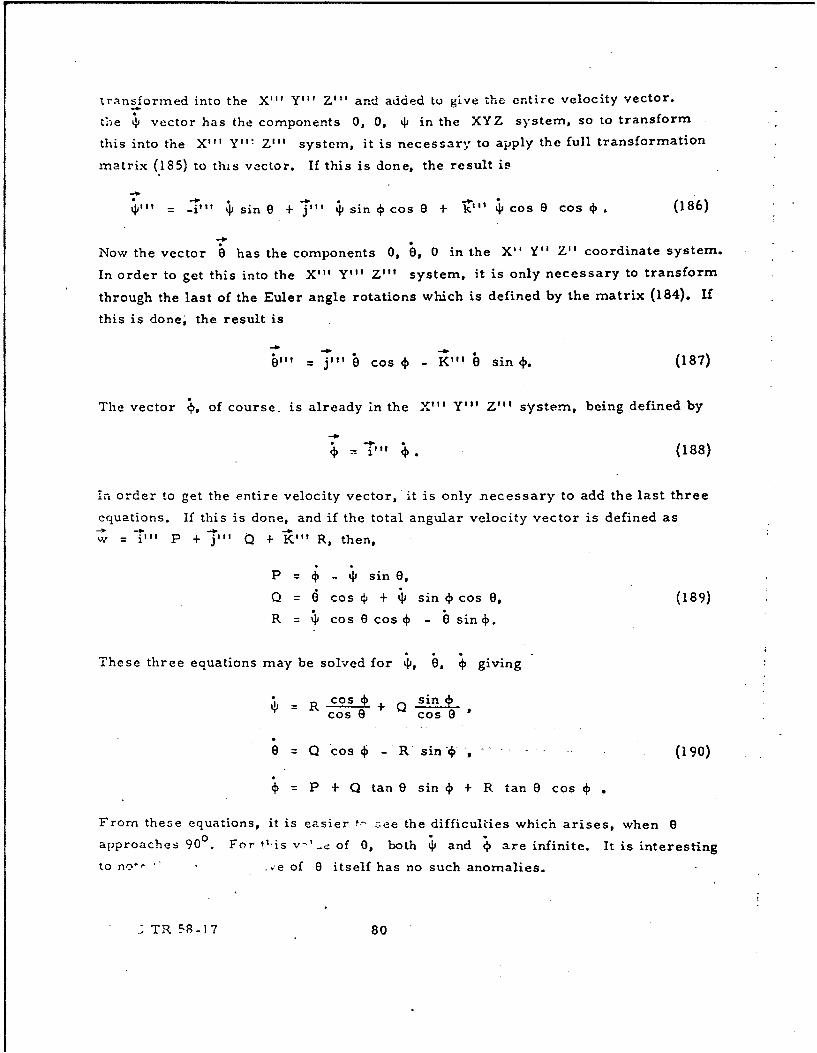
transformed into the X'" Y"' Z" and added to give the entire velocity vector.
the ý vector has the components 0, 0, q) in the XYZ system, so to transform
this into the X'" Y"' Z'" system, it is necessary to apply the full transformation
matrix (185) to this vector. If this is done, the result is
" = -i"i' sin 0 + j"' • sin • cos 0 + i"' , cos 0 cos * (186)
Now the vector 8 has the components 0, 8, 0 in the X" Yi" Z'I coordinate system.
In order to get this into the X"' Yln" Z1" system, it is only necessary to transform
through the last of the Euler angle rotations which is defined by the matrix (184). If
this is done, the result is
"b"ll = j"1 0 Cos - Ki'l sin (. (187)
The vector •, of course, is already in the X"' Y'" Z"' system, being defined by
il l, . (188)
:n order to get the entire velocity vector, it is only necessary to add the last three
equations. If this is done, and if the total angular velocity vector is defined as
w = il' P + j"' 0 + Kill R, then,
P = - 4 sin 0,
Q = cos 4 + sin cos 6, (189)
R 4= cos0o - Osin4,.
These three equations may be solved for 4, 0, 4 giving
R Cos 4b sin4cos 8 cos 0
8=Q cos -Rsin , R... . (190)
4, = P + Q tan 0 sin +, 4- R tan 0 cos 4.
From these equations, it is easier t- -•ee the difficuldies which arises, when 0
approaches 90 o. For tOis v-'-e of 0, both 4l and ; are infinite. It is interesting
to no", -e of 0 itself has no such anomalies.
TR 58-17 80
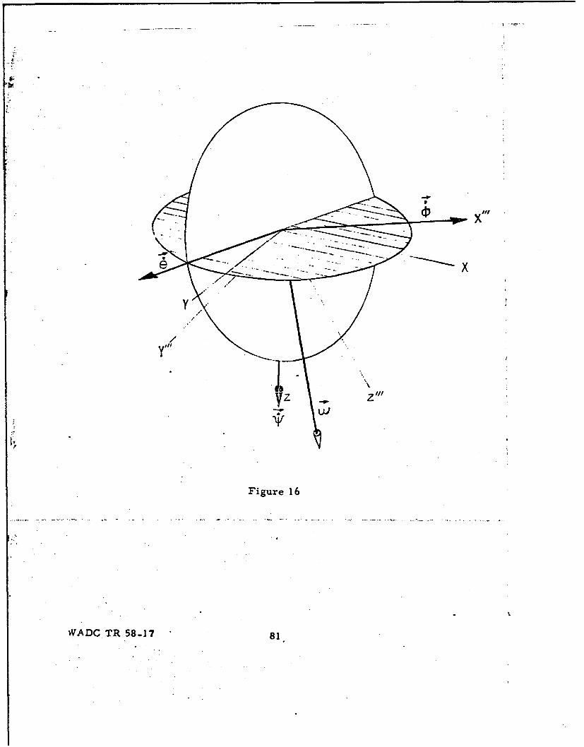
Figure,1
WADC R 5817 8
APPENDIX C
SERVOMULTIPLIER ERRORS
In the past, it has evidently not been the practice to treat analog multiplier
errors, with much care in error analyses. The usual procedure has been to
assume some upper bound for the error and to consider the error constant at that
value. This, of course, gives a pessimistic view of 4the results to be expected,
though in many cases this is not undesirable, and it certainly gives an estimate of
the order of magnitude of the resultant error. Possibly the principal reason that
errors are not treated with more care is that little is known about their detailed
character. No two multipliers are the same, a given multiplier will change with
time, and it is a great bother to measure the errors anyhow. It would appear,
then, that a statistic d approach is indicated. If the statistical distribution of
errors can be establi. hed, then it can be used to predict the distribution of errors
in the problem result. This will not give a measure of the error in any particular
run, but it is not practical to do this in any event. It would appear that if we know
the distribution of errors in the solution, it is fair to say that we know all that is
necessary about those errors.
It will become clear that the statistical procedures applied in this work are of
the very simplest sort. Many more things could have been done, even with the data
which were taken, but it was not felt to be worthwhile. The prinicpal reason for this
is that, as was pointed out earlier, multiplier errors did not turn out to be the
principal source of drift in the coordinate conversion simulation. Therefore, it was
not possible to check the predicted error distribution against the observed distribu-
tion, even to the extent permitted by the small number of samples available.
Generally speaking, the procedure was to take an average of all errors of all
multipliers over their entire range; taking the average in a manner generally
consistent with the way the multipliers are used in the coordinate conversion simu-
latinn. It was assumcd that the error voltage was directly- proportional to- the voltage
acros& the multiplying potentiometer, and this was kept at ± 100 volts throughout
the measurements. Once the error distribution is established for this case, it is
possible to get the distribution for ;-ny other pot voltage by simnply multiplying the
J- 100 volt distribution by V/f900, where V is the pot voltage.
ADC TR 58-17 82
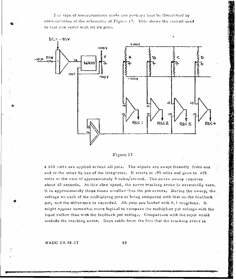
T, .O type of rne'I'surements .n:ade carn prh-ips be ot b, i]luiti'ated by
conrce'e.,tion of the -;chel iatic of trig~uri 17. This shows the circuit uscd
to tvst one serve with all its pots.
I.0 -5
4 iOO\1 ._____
41001'
to o
Figure 17
a 100 volts are applied across all pots. The wipers are swept linearly from one
end to the other by use of the integrator. It starts at -95 volts and goes to +95
volts a- the rate of approximately 5 voits/second. The entlirre wcu/p r'tequirct;
about 40 seconds. At this slow speed, the servo tracking error is essentially zero.
It is approximately three times sinaller ':han the pot errors. During the sweep, the
voltage on each of the multiplying pots is being compared with that ori the feedback
pot, ar.d the difference is recorded. Ali pots are loaded with 0, 1 rnegehms. It
might appear somewhat more logical to compare the multiplier 'zOt voltage with the
input rather than with the feedback pot voltage. Comparison with the input would
include th- tracking error. Elven aside from the fact that the tracking error is
5
WADC "rR 58-17 83[
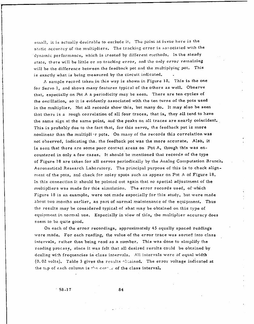
snmall, it is actually desirable to exclude it. The point at issue here is the
s':ztic accuracy of the multipliers. The tracking error is asF.ociated with the
dynamic performance, which is Lreated by different nmethods. In the steady
state, there will be little or no tracking error, and the only error remaining
will be the difference between the feedback pot and the multiplying pot. This
is exactly what is being measured by the circuit indicated.
A sample record taken in this way is shown in Figure 18. This is the one
for Servo 1, and shows many features typical of the others as well. Observe
that, especially on Pot A a periodicity may be seen. There are ten cycles of
the oscillation, so it is evidently associated with the ten turns of the pots used
in the multiplier. Not all records show this, but many do. It may also be seen
that there is a rough correlation of all four traces, that is, they all tend to have
the same sign at the same point, and the peaks on all traces are nearly coincident.
This is probably due to the fact that, for this servo, the feedback pot is more
nonlinear than the multipli -r pots. On many of the records this correlation was
not observed, indicating tha. the feedback pot was the more accurate. Also, it
is seen that there are some poor contact areas on Pot A, though this was en-
countered in only a few cases. It should be mentioned that records of the type
of Figure 18 are taken for all servos periodically by the Analog Computation Branch,
Aeronautical Research Laboratory. The principal purpose of this is to check align-
ment of the pots, and check for noisy spots such as appear on Pot A of Figure 18.
In this connection it should be pointed out again that no special adjustment of the
multipliers was made for this simulation. The error records used, of which
Figure 18 is an example, were not made especially for this study, but were made
about twvo months earlier, as part of normal maintenance of the equipment. Thus
the results may be considered typical of xhat may be obtained on this type of
equipment in normal use. Especially in view of this, the multiplier accuracy does
seem to be quite good.
On each of the error recordings, approximately 45 equally spaced readings
were made. For each reading, the value of the error trace was sorted ;into class
intervals, rather than being read as a number. This was done to simplify the
reading process, since it was felt that all desired results could be obtained by
dealine with frequencies in class intervals. All intervals were of equal width
(0. 02 volts). Table 3 gives the results -ý!'ained. The error voltage indicated at
the tcp of Each column is tl•e cer' of the class interval.
"58-17 84
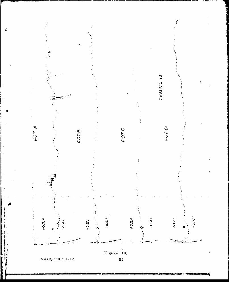
IL A'I
-i 0
Fiue 8
VVAD TR. 58178
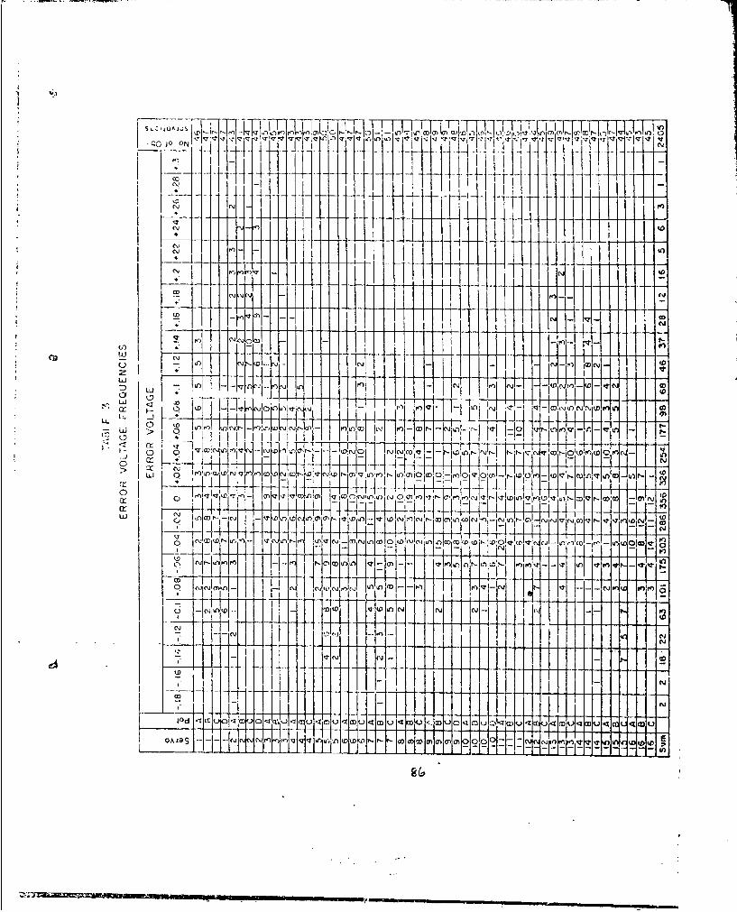
U) Inw~ -- -) -- kI I- _ _ U. u-*'
Icli
U)
I1 I Q ,1 CD Il TjiJ~ N
_Y I
LU to
~
*-;~ ~ ~ ~ ~~I r~~:- ~I m~~ N\ ~,DDb- bo(if - N-~OD t- 2 OIn~
0Aa 7. 01r~ -T~ l~f (0C)!!~7 00 -
LL) D I ýz , L 0 (T- IT O v W M i ci 11 icj V)1-6
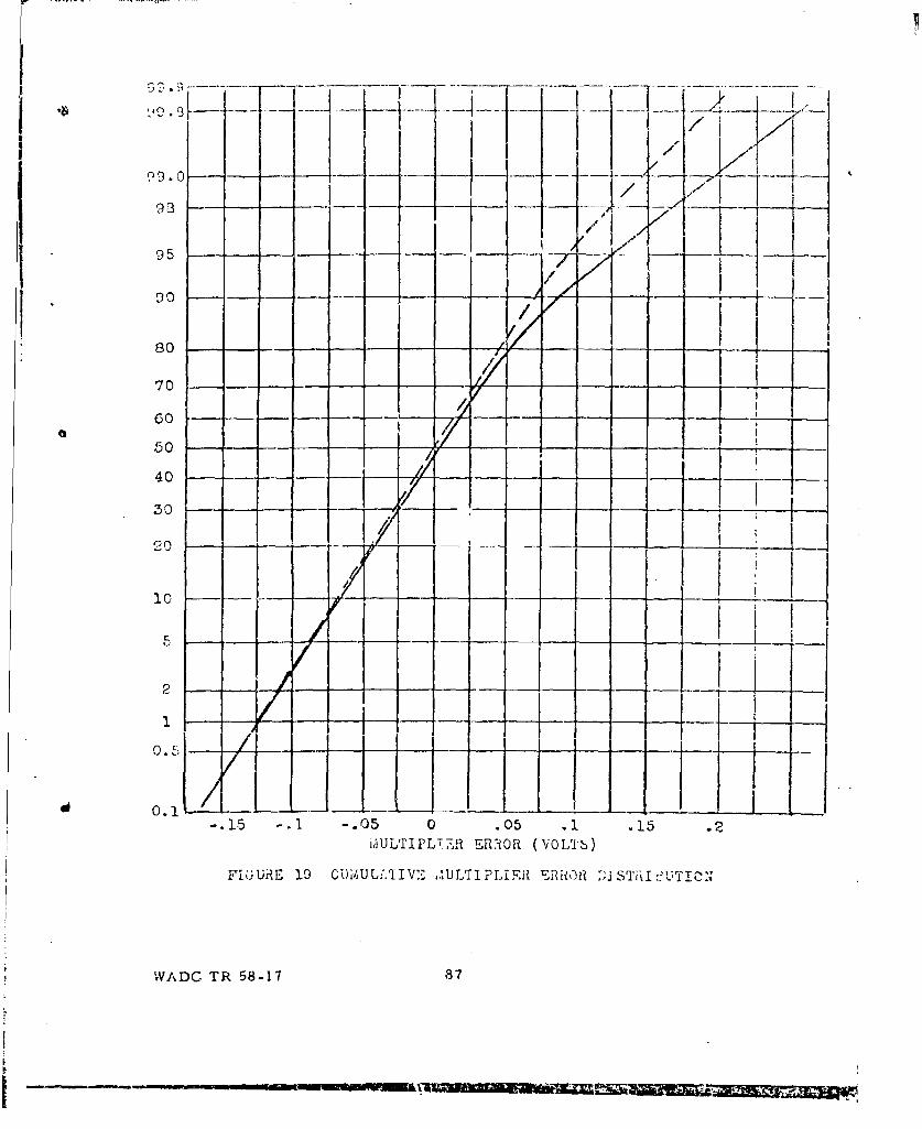
90 ~-
80 0,
50-
40-- --
30 - - - * - -fF
2 ii
-. 15 .1 -. 05 0 .05 .1 .15 .ji~ULTIPLT7Rf UR.ýOR (VOLTS))
F16UiiE 19 CUAIUL;.TIVE ..lULTIPLIFUI R Dl Sjjij I j ~
WADC TR 58-17 87
WIER
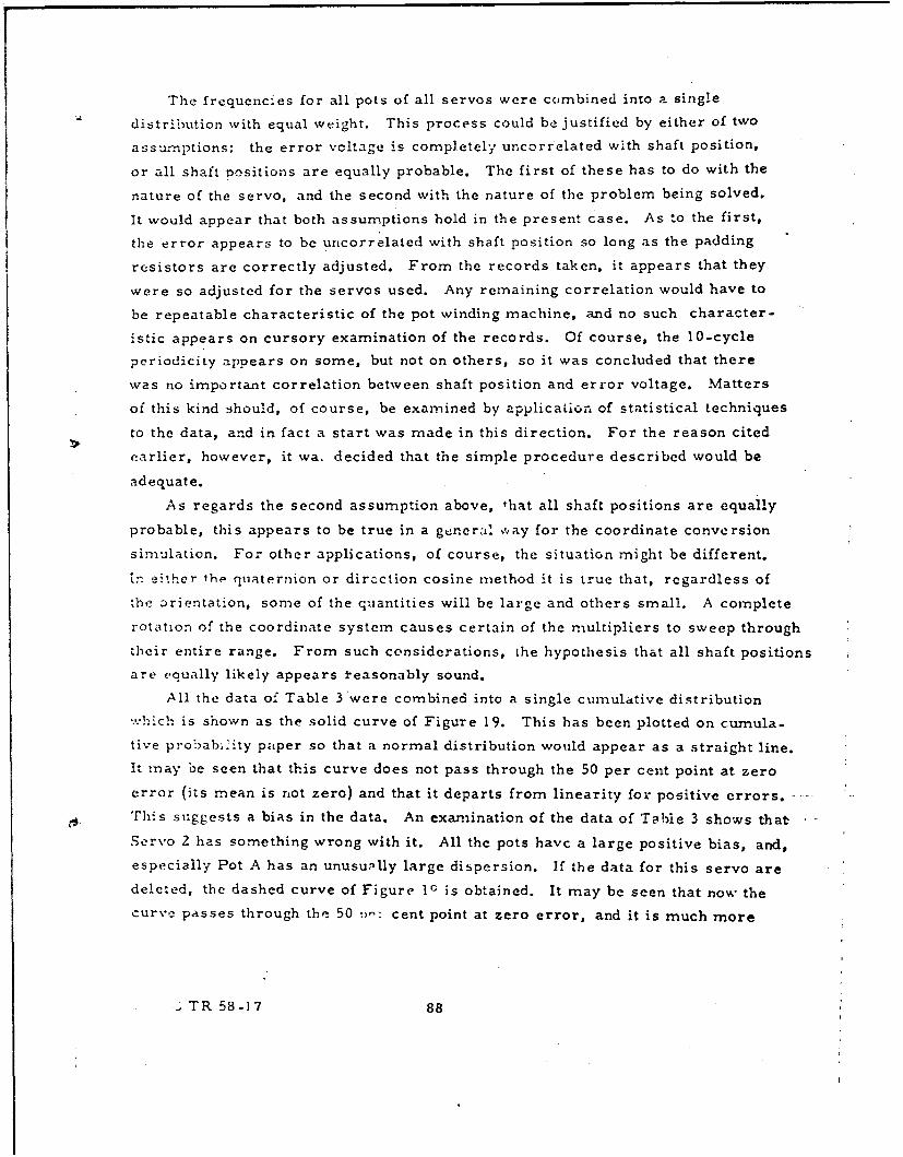
The frequencies for all pots of all servos were combined into a single
distribution with equal weight. This process could be justified by either of two
assumptions: the error voltage is completely ur,correlated with shaft position,
or all shaft positions are equally probable. The first of these has to do with the
nature of the servo, and the second with the nature of the problem being solved.
It would appear that both assumptions hold in the present case. As to the first,
the error appears to be uncorrelated with shaft position so long as the padding
resistors are correctly adjusted. From the records taken, it appears that they
were so adjusted for the servos used. Any remaining correlation would have to
be repeatable characteristic of the pot winding machine, and no such character-
.stic appears on cursory examination of the records. Of course, the 10-cycle
periodicity appears on some, but not on others, so it was concluded that there
was no important correlation between shaft position and error voltage. Matters
of this kind should, of course, be examined by application of statistical techniques
to the data, and in fact a start was made in this direction. For the reason cited
narlier, however, it wa. decided that the simple procedure described would be
adequate.
As regards the second assumption above, that all shaft positions are equally
probable, this appears to be true in a genera. Yay for the coordinate conversion
simulation. For other applications, of course, the situation might be different.
Tn either thl, quaternion or direction cosine method it is true that, regardless of
the orientation, some of the quantities will be large and others small. A complete
rotation of the coordinate system causes certain of the multipliers to sweep through
their entire range. From such considerations, the hypothesis that all shaft positions
are equally likely appears i'easonably sound.
All the data of Table 3 were combined into a single cumulative distribution
,'Thich is shown as the solid curve of Figure 19. This has been plotted on cumula-
tive probabýi;ty paper so that a normal distribution would appear as a straight line.
It may be seen that this curve does not pass through the 50 per cent point at zero
error (its mean is riot zero) and that it departs from linearity-for po-si-tive errors.
This suggests a bias in the data. An examination of the data of Table 3 shows that.
Servo 2 has something wrong with it. All the pots havc a large positive bias, and,
especially Pot A has an unusually large dispersion. If the data for this servo are
deleted, the dashed curve of Figure 1c is obtained. It may be seen that now the
curve passes through the 50 r•: cent point at zero error, and it is much more
TR 58-17 88
nearly a straight line. There is still some deviation from linearity, and this
is no doubt due to bias in somc of the pots, but it appears that the errors may
be represented reasonably well by a normal distribution. The standard devia-
tion may be determined from the value at which the curve crosses the 84. 15 per
cent line. This turns out to be 0. 053 volts..
In the error analysis, then, it may be assumed that the multiplier errors are
normally distributed, with a sandard deviation of 0. 053 volts, when the voltage
across the rmultiplying pot is 1 100 V. It would be proportionately less for smaller
pot voltages.
WADC TR 58-17 89


![Quadratic Split Quaternion Polynomials: …...been done for quaternions in [6] and for split quaternions in [2]. Results for generalized quaternions, including split quaternions, can](https://img.pdfslide.us/doc/110x75/5ea3ed9b0e257f05c666f8d7/quadratic-split-quaternion-polynomials-been-done-for-quaternions-in-6-and.jpg)