Embed Size (px)
Citation preview

Simulation of High-velocity Penetration for Rigid Projectile into Plain Concrete Target using
Discrete Element Method
Yu ZHOU
Thesis submitted to the faculty of
Virginia Polytechnic Institute and State University
in partial fulfillment of the requirements for the degree of
Master of Science
In
Civil Engineering
Linbing Wang, Chair Gerardo W. Flintsch Antoine G. Hobeika
February 4, 2009
Blacksburg, Virginia
Keywords: Penetration, DEM, Simulation, Calibration
Copyright 2009, Yu ZHOU

Simulation of High-velocity Penetration for Rigid Projectile
into Plain Concrete Target using Discrete Element Method
Yu ZHOU
(ABSTRACT)
Penetration of high velocity is of concern for both civilian and military research for
decades, and computerized simulation is the scholar’s focus in recent years. This
study presents a study on the Discrete Element Method (DEM) simulation of plain
concrete target’s behavior under high-velocity penetration of rigid projectile.
In this thesis, different types of research works including empirical, analytical and
numerical methods in penetration by the previous scholars were carefully reviewed. A
DEM-based concrete model was established by using software PFC3D. The major
micro-variables of the simulation program were calibrated according to the required
macro-mechanical parameters. Meanwhile, their correlations within the concrete
range were studied, with the sensitivity analysis and the corresponding regression
equations.
With the established digital concrete model, penetration simulation tests were carried
out. The results of penetration depth versus impact velocity were compared with the
experimental and empirical calculated results from Forrestal’s work in 1994. A good
agreement was obtained. Some other simulation studies, like projectile mass,
geometry, penetrating acceleration, concrete response stress, strain, and strain-rate
were also conducted to study the constitutive properties in this thesis.

III
This thesis is dedicated to my parents Jianguo ZHOU and Xiaoqin HE

IV
ACKNOWLEDGEMENT
The author wants to thank his advisor, Dr. Linbing Wang for his support and
patient supervision. His valuable and constructive advice and comments are greatly
appreciated.
The author also wants to thank his advisory committee members, Dr. Gerardo
W. Flintsch, and Dr. Antoine G. Hobeika, for their valuable advices and support
during coursework and thesis preparation.
The author would like to thank his colleagues and friends for their help both in
and out of office and laboratory.
The research was made possible with the support from the Department of Civil
and Environmental Engineering and VTTI of Virginia Tech.

V
TABLE OF CONTENT
Chapter 1. Introduction .............................................................................................................. 1
1.1. Research Background .................................................................................................... 1
1.2. Research Objectives ...................................................................................................... 1
1.3. Research tasks and organization ................................................................................... 2
Chapter 2. Literature Review ...................................................................................................... 4
2.1. Penetration Introduction ............................................................................................... 4
2.1.1. Basics about penetration and the focus of this thesis ...................................... 4
2.1.2. Key parameters for penetration ........................................................................ 5
2.2. Methodologies for penetration study ........................................................................... 6
2.2.1. Empirical methods............................................................................................. 7
2.2.1.1. Normal penetration case studies .............................................................. 7
2.2.1.2. Special penetration cases study .............................................................. 13
2.2.2. Analytical methods .......................................................................................... 15
2.2.3. Numerical methods ......................................................................................... 21
2.2.3.1. FEM application in penetration ............................................................... 22
2.2.3.2. DEM for penetration simulation ............................................................. 23
Chapter 3. Methodology used for this Study ............................................................................ 27
3.1. PFC3D and its Fundamental theorem ......................................................................... 27
3.1.1. Particle‐Flow model ........................................................................................ 27
3.1.1.1. Force‐Displacement Law ......................................................................... 28
3.1.1.2. Law of Motion ......................................................................................... 29
3.2. Contact models applied in this study .......................................................................... 29
3.2.1. Contact‐stiffness model (linear) ...................................................................... 30
3.2.2. Slip model ........................................................................................................ 30
3.2.3. Bonding model (parallel) ................................................................................. 31
3.3. Parameters Definition and Inputs ............................................................................... 33
3.4. Digital Model Creation for Projectile and Target ......................................................... 34
3.4.1. Projectile Model .............................................................................................. 34
3.4.2. Target Model ................................................................................................... 36
Chapter 4. Calibration of micro‐variables in Digital Concrete and Sensitivity Analysis ............ 40
4.1. Theories for the Calibration Test simulation ............................................................... 40
4.2. Individual Effect of major Micro‐variables .................................................................. 42
4.2.1. Calibration of microscopic elastic modulus ..................................................... 42
4.2.2. Calibration of microscopic normal over shear stiffness ratio .......................... 45
4.2.3. Calibration of Normal and shear strength for parallel bond ........................... 48
4.2.4. Calibration of friction among particles ............................................................ 52
4.3. Multi‐Effect Analysis and Regression Development .................................................... 54
4.3.1. Young’s Modulus ............................................................................................. 54
4.3.2. Poisson’s Ratio ................................................................................................. 56
4.3.3. Compressive Strength ..................................................................................... 58
4.3.4. Summary of the macro‐micro regression equations ....................................... 64
Chapter 5. Simulation Results and Analysis .............................................................................. 65

VI
5.1. Visualization of DEM penetration simulation.............................................................. 65
5.2. Velocity‐Depth Test Validation and related factor analysis ......................................... 67
5.3. Microscopic Stress and strain relationship .................................................................. 71
5.3.1. Stress‐strain relationship and related crack history record ............................. 72
5.3.2. Elastic moduli – strain rate relationship analysis ............................................ 74
5.3.3. Stress distribution and time relation ............................................................... 77
Chapter 6. Summary and Conclusions ...................................................................................... 80
6.1. Scientific accomplishments ......................................................................................... 80
6.2. Limitation of the methodology in this thesis .............................................................. 80
6.3. Recommendation for the further study ...................................................................... 81

VII
LIST OF FIGURES
Figure 2‐1. Projectile response after impact (Cargile 1999) ...................................................... 4
Figure 2‐2. The geometry of projectile nose shape (Chen and Li 2002) ................................... 6
Figure 2‐3. Geometry and response regions of cavity expansion theory (Forrestal 1986), with
c, c1‐ interface velocities, cd‐ elastic, dilation velocity ..................................................... 17
Figure 2‐4. Close‐pack of particles (Nishida et al. 2004) ......................................................... 24
Figure 2‐5. Different sizes of particles (Ng 1993) .................................................................... 24
Figure 2‐6. Reinforcement layer of concrete slab using DEM element (Magnier and Donze
1998) ............................................................................................................................... 25
Figure 3‐1. Procedure of each DEM calculation cycle ............................................................. 28
Figure 3‐2. Contact stiffness model for ball‐ball and ball‐wall (Itasca Consulting Group 2005)
......................................................................................................................................... 29
Figure 3‐3. Schematic of parallel bond (Itasca Consulting Group 2005). ................................ 31
Figure 3‐4. Existing condition of different contact models in DEM of PFC3D ......................... 33
Figure 3‐5. The geometry of projectile used in test (Forrestal et al. 1994) ............................. 34
Figure 3‐6. Projectile model created in DEM .......................................................................... 36
Figure 3‐7. Model concrete target (The outer side of target particles are set fixed as the
boundary, in color blue to simulate the fixation of real test) .......................................... 38
Figure 4‐1. Uniaxial tests display ............................................................................................. 40
Figure 4‐2. Relation between axial stress, confining stress and axial strain in uniaxial test ... 41
Figure 4‐3. Relation between Young’s modulus and micro‐elastic modulus........................... 43
Figure 4‐4. Relation between Poisson’s ratio and micro‐elastic modulus ............................... 44
Figure 4‐5. Relation between Poisson’s ratio and micro‐elastic modulus ratio ...................... 44
Figure 4‐6. Relation between Compressive strength and micro‐elastic modulus ................... 45
Figure 4‐7. Relation between Poisson’s ratio and micro‐kn/ks ............................................... 46
Figure 4‐8. Relation between Young’s modulus and micro‐kn/ks ........................................... 47
Figure 4‐9. Relation between Compressive strength and micro‐kn/ks ................................... 47
Figure 4‐10. Relation between Compressive strength and micro‐strength ............................ 49
Figure 4‐11. Relation between Compressive strength and micro‐strength ............................ 49
Figure 4‐12. Relation between Compressive strength and micro‐strength ............................ 50
Figure 4‐13. Relation between Young’s modulus and micro‐strength .................................... 51
Figure 4‐14. Relation between Poisson’s ratio and micro‐strength ........................................ 51
Figure 4‐15. Relation between Young’s modulus and friction ................................................ 53
Figure 4‐16. Relation between Poisson’s ratio and friction ..................................................... 53
Figure 4‐17. Relation between Compressive strength and friction ......................................... 53
Figure 4‐18. Combined effects of Ec and pb_Ec on Young’s Modulus .................................... 55
Figure 4‐19. Combined effects of friction and pb_kn/ks on Young’s Modulus ....................... 55
Figure 4‐20. Combined effects of friction and pb_kn/ks on Poisson’s ratio ............................ 56
Figure 4‐21. Combined effects of pb_kn/ks and Ec/pb_Ec on Poisson’s ratio ........................ 57
Figure 4‐22. Combined effects of Ec/pb_Ec and friction on Poisson’s ratio ............................ 57
Figure 5‐1. Visualization of the penetration process (with the 2nd and 3rd step enlarged) .. 65
Figure 5‐2. Visualization of the change of projectile velocity, penetration depth, and
corresponding projectile‐target friction in the penetration process .............................. 66

VIII
Figure 5‐3. Penetration depth of the projectile for both simulation and empirical prediction
......................................................................................................................................... 66
Figure 5‐4. Acceleration of the projectile for both simulation and empirical prediction........ 67
Figure 5‐5. Velocity of the projectile for both simulation and empirical prediction ............... 67
Figure 5‐6. Relationship between final penetration depth and impact velocity for test,
empirical equation and DEM simulation ......................................................................... 69
Figure 5‐7. Correlation between penetration depth and projectile mass under 500m/s
impact velocity ................................................................................................................ 70
Figure 5‐8. Correlation between penetration depth and projectile tail diameter under impact
velocity 500m/s ............................................................................................................... 70
Figure 5‐9. Comparison of penetration Simulation with different friction factor ................... 71
Figure 5‐10. Illustration of the measurement of stress and strain .......................................... 72
Figure 5‐11. Relation between stress and strain for specified position z=‐0.2m (0.25m from
the projectile face) at 500m/s impact velocity ................................................................ 72
Figure 5‐12. Relation between crack and radial strain at 500m/s impact velocity ................. 73
Figure 5‐13. Relation between cracks number and time at 500m/s impact velocity .............. 74
Figure 5‐14. Relation between cracks number and penetration depth at 500m/s impact
velocity ............................................................................................................................ 74
Figure 5‐15. Relation between radial stress and strain ........................................................... 75
Figure 5‐16. Relation between radial stress and time ............................................................. 75
Figure 5‐17. Relation between radial stress and penetration depth ...................................... 75
Figure 5‐18. Relation between average elastic modulus and strain rate ................................ 76
Figure 5‐19. Illustration of the four measurement locations on the cross section of the target
......................................................................................................................................... 77
Figure 5‐20. Illustration of the specified measurement depth in the target (The projectile of
this illustration is not to scale) ........................................................................................ 77
Figure 5‐21. Distribution of velocity in z‐direction along radius ............................................. 78
Figure 5‐22. Distribution of radial stress along radius and depth ........................................... 79
Figure 5‐23. Variation of radial stress over the whole penetration process ........................... 79

IX
LIST OF TABLES
Table 2‐1. Values of A, B, C of CET models with different assumptions (Forrestal and Tzou
1997) ............................................................................................................................... 19
Table 2‐2. Summary of different methods used for penetration study before 1990 .............. 22
Table 2-3. Key features for DEM study in penetration by different researchers since 1990 .. 26 Table 3‐1. Equations of force and moment for parallel bond and corresponding parameters
......................................................................................................................................... 32
Table 3‐2. Key variables in different contact constitutive models in PFC3D ........................... 33
Table 3‐3. Material properties for both projectile and the target (Forrestal et al. 1994) ....... 35
Table 3‐4. Example of micro‐variables in digital projectile ..................................................... 35
Table 3‐5. Corresponding macro‐parameters for digital projectile ......................................... 35
Table 3‐6. Example of micro‐variables in concrete target creation ......................................... 37
Table 3‐7. Corresponding macro‐parameters for digital concrete target ................................ 37
Table 4‐1. Macro‐parameters for concrete and the corresponding major micro‐variables .... 41
Table 4‐2. Calibration of micro‐elastic modulus (contact‐stiffness and parallel‐bond modulus)
......................................................................................................................................... 43
Table 4‐3. Calibration of micro‐kn/ks (contact‐stiffness modulus and parallel‐bond modulus)
......................................................................................................................................... 46
Table 4‐4. Calibration of micro‐strength (normal and shear strength for the particle) .......... 48
Table 4‐5. Calibration of friction among particles ................................................................... 52
Table 4‐6. Individual effects of micro‐variables on Compressive Strength ............................. 58
Table 4‐7. Combined effects of micro‐variables on Compressive Strength ............................. 61
Table 4‐8. Regression equations for compressive strength ..................................................... 63
Table 4‐9. Regression equations summary for different macro‐parameters .......................... 64
Table 5‐1. Macro‐parameters and micro‐variables for the test and digital concrete .............. 68
Table 5‐2. Relation between final penetration depth and impact velocity for test, empirical
equation and DEM simulation ......................................................................................... 69
Table 5‐3. Relation between average elastic modulus and strain rate, with corresponding
impact velocity and final penetration depth ................................................................... 76

1
Chapter 1. Introduction
1.1. Research Background
Penetration of high velocity projectiles into concrete targets is a concern of
both civilian and military research. The earliest study of penetration mechanics can be
traced back to 300 years ago; however, it is World War II that triggered the systematic
focus into this specialty.
Numerical simulation of penetration comes with the application of Finite
Element Method (FEM) and Discrete Element Method (DEM). FEM has been used
widely since the 1970s, while DEM only became the popular since 1990s. There is
not much study of DEM application in the penetration research.
1.2. Research Objectives
The objective of this thesis is to make use of DEM to simulate the normal
high-speed penetration into semi-infinite plain concrete target. Detailed purposes are:
1. Build up a DEM digital concrete model with PFC3D.
2. Calibrate the key microscopic variables according to the macroscopic
properties, conduct the sensitivity analysis, and get the correlation regression
equations.
3. Use the calibrated digital concrete model to simulate the test of normal
high-speed penetration.
4. Carry out a vast quantity of simulation tests to study the correlation between
the penetration depth and other key factors, such as the impact velocity and the shape
of projectile.

2
5. Compare simulation results with experimental results and those from
empirical theory, through the use of diagrams representing depth-velocity.
6. Study the constitutive relation under different dynamic conditions
1.3. Research tasks and organization
This thesis is organized into five chapters:
Chapter 1 describes the background of the study, clarifies the research
objective, and explains the organization of this thesis.
Chapter 2 presents the review of relevant literature for this study. The first part
introduces the basics and the key parameters of the penetration study, while the
second part focuses on several methodologies for penetration study completed by
previous scholars, which are classified into empirical, analytical, and numerical
methods.
Chapter 3 introduces the simulation method applied in this report. PFC3D is
the software used for the modeling, while DEM was the theory behind it. The
fundamental rules for DEM (force-displacement law, motion law, and contact models)
are explained first. Then the sample key variables setting for both projectile and target
are listed in the next section, followed by the corresponding sample digital model.
Chapter 4 is about one of the major work completed in this thesis. The
individual and multi effect of the major micro-variables in PFC programming have
been studied, provided with the sensitivity analysis and the corresponding regression
equations. Based on these principles discovered, a calibration has been conducted for
the digital concrete material to obtain the required mechanical property.
On the basis of the calibrated projectile and target model, a penetration
simulation model is presented and in Chapter 5. With this model, series of simulation
test have been conducted. Not only the visualization of the whole process is shown,

3
but also the history record of monitored internal variables have been kept. Among
them, the penetration depth-impact velocity correlation has been used to validated the
established digital model through the comparison with the experiment and empirical
results done by the previous work. And the stress-strain correlation have been studied,
which shows that the mechanical property of concrete is rather a rate-dependent term
not static.
Chapter 6 summarizes the findings and limitations of this thesis, and provides
recommendations for further study.

4
Chapter 2. Literature Review
2.1. Penetration Introduction
2.1.1. Basics about penetration and the focus of this thesis
Due to the various impact conditions and target properties, the injection of a
projectile into a target can be divided into different response types, as seen in Figure
2-1. Among them, the normal impact strike type receives the most concern. There are
three possible results (Cargile 1999) depending on the impact energy on the target:
1. Impact- the strike only forms an impact crater;
2. Deep Penetration- the projectile goes over the crater, forms a tunnel, and is
finally embedded in the target;
3. Perforation- the projectile pierces the target of finite thickness, while the
whole process creates an impact crater, a tunnel, and an exit crater.
Figure 2-1. Projectile response after impact (Cargile 1999)
Most research focuses on deep penetration (usually idealizing the target as a
semi-infinite body in the theoretical study), which is dominated by severe compaction,
shear, and tension. The principal force takes effect at the resistance around the

5
projectile nose, while the extremely high stress in the neighboring area decreases
rapidly away from the cavity.
Other special types of impact are considered non-ideal, such as ricochet,
broach (due to oblique impact), breaking up (due to low strength of penetrator), yaw,
moving target, rotating or tumbling, etc. These types also include phenomenon as
detailed in Goldsmith’s summary review (Goldsmith 1999). Considered, however,
these special cases are not.
2.1.2. Key parameters for penetration
There are many important characteristics of both target and projectile that
affect penetration results. These features determine the constitutive relationship of
both entities. Below are some typical parameters for penetration research and their
typical values discovered in the past studies.
For the target:
1. Dimension: semi-infinite (applied to deep penetration); Finite (applied to
perforation, especially when people are interested in the phase of exit crater).
2. Material type: metal; composite (such as concrete); geomaterial (such as
rock, soil, frozen soil, sediment, and etc), ice, and layered material.
3. Mechanical property, which is related with the material type: elastic
modulus, poisson’s ratio, and strength (compressive and tensile).
For the projectile:
1. Impact velocity;
2. Impact angle to the target (normal, oblique);
3. Mass;

6
4. Strength (rigid, deformable);
4. Geometry (tail diameter, nose shape as seen in Figure 2-2).
Figure 2-2. The geometry of projectile nose shape (Chen and Li 2002)
2.2. Methodologies for penetration study
F. E. Heuze (Heuze 1990) provided a comprehensive and valuable summary of
the penetration studies conducted before 1990. Heuze’s summary focused on
geological material, especially rocks, and classified all the methodologies into the
empirical, the analytical, and the numerical simulation methods. It covered nearly all
the important methods on penetration research. Due to the similarity of constituents
and mechanics between concrete and rocks, his classification system is utilized in this
study.
The applications of different methodologies vary according to the research
range and depth. The empirical method provides the simplest and easiest way to
obtain the macroscopic factors, such as penetration depth; the analytical method can
provide answers for not only the direct observable parameters, but also some other
properties, such as stress and strain relationship; and the numerical simulation could
offer the detailed description of the entire penetration process from all aspects, yet
sometimes not precisely consistent with the experimental observations.
In addition to describing the existing models, Heuze (Heuze 1990) also
compared the different methods. His conclusions drawn on the overview of the whole

7
study area include:
1. Cracks and joints are ubiquitous and damage characterization should be
incorporated in the modeling and simulation;
2. Shear strength is sensitive to the mean stress, and yielding strength should
be mean stress dependent;
3. Post-fracture properties of the broken material are also essential and the
interaction among the fragments should be considered;
4. The internal friction angle of the target is more important than its cohesive
strength in controlling penetration.
2.2.1. Empirical methods
The Empirical methods may be the oldest and most direct. They are based on
the experimental data, and usually apply mathematical tools like regression to get an
empirical relation. The wide use of empirical methods is due to their simplicity and
good correlation with test results, which enables a quick first approximation and
comparison to other methods.
2.2.1.1. Normal penetration case studies
M.E.Backman (Backman and Goldsmith 1978) included some examples of
empirical formulae developed by the scholars in the 19th century as shown below. It
is noticeable that some typical parameters are concern of different researchers, such as
P - penetration depth; m – projectile mass; v0 - the impact velocity; θ- obliquity and
the type of target and its thickness h0; D - projectile tail diameter; E0 - required
perforation energy,ρt - target density; ai - arbitrary constants.
Morin (1833)’s equation
2 30 1/ 2 /P D mv a Dπ= 2-1

8
Dideon’s equation
22 3 0/ ln(1 )tP D a a vρ= + 2-2
Helie’s equation
3 24 10 5 0/ (4.608 / ) log (1 )tP D m a D a vπρ= + 2-3
where
P - penetration depth;
m – projectile mass;
v0 - the impact velocity;
θ - obliquity and the type of target and its thickness h0;
D - projectile tail diameter;
E0 - required perforation energy,
tρ - target density;
ai - arbitrary constants.
All of these equations are based on the semi-infinite (SI) target.
The Army’s Waterways Experiment Station (WES), Vicksburg (Bernard 1977;
Bernard 1978) developed their formulae for penetration research, which is another
important reference in the last 20 years. Its theory incorporate a characteristic
parameter, Rock Quality Designation (RQD), the percent of total core length made up
of pieces at least 4 inches long. This parameter needs to be back-calculated from the
penetration tests. A typical penetration depth equation is shown below.

9
1/2 1/2
1/2 1/2
4 3[ ln(1 )]3 9 4
rc
cr cr
NM VZ VA
ρ ρρ σ σ
= − + 2-4
where
rcN - The projectile nose performance coefficient
21/4
1/2
4( )0.863[ ]4 1
0.805(sin )
rc
rc c
CRHNCRH
N η −
⎧=⎪
−⎨⎪ =⎩
forfor
__
ogive nosecone nose
0.2( / 100)cr c RQDσ σ=
M - the concrete mass
crσ - the unconfined compressive strength
cη - the cone half-angle
Rock Quality Designation (RQD), also used in concrete, is calculated as the
percent of total core length made up of pieces at least 4 inches long. Compared to Q,
the shortcoming of RQD is that its magnitude is dominated by horizontal cracks.
Another depth formula was developed in 1992 by WES.
1.8
1.8 0.5
222* * ** 'c
N W VX DD f
= + ; for X>2D 2-5
where
0.50.72 0.25( 0.25)N CRH= + −
X - penetration depth, inch
fc’ - compressive strength of concrete, psi

10
N - nose shape factor or nose performance coefficient
W - projectile weight, lb
D - projectile diameter, inch
V - impact velocity/1000, fps
Sandia National Laboratories (SNL) in Albuquerque, New Mexico plays a
very important part in the penetration study. Among the researchers there, Young,
C.W and his colleagues (Young 1967; Young 1972; Schoof, et al. 1989; Young 1998)
developed their empirical models and continued their work into diverse kinds of
conditions. In 1997, Young summarized his previous work done in penetration,
covered in his paper all prediction equations he developed for different penetrator
nose shape (ogive, conic, blunted), impact velocities (<200fps, ≥200fps), types of
targets (rock, concrete, ice, and the layered target). Young’s equations have been
incorporated into different program codes, like SAMPLL code and MOLE code,
which enable efficient penetration modeling.
The Penetration Depth equations for uniform layer or half space of concrete
0.7 2 5
0.7
0.3 ( / ) ln(1 2 10 )0.00178 ( / ) ( 100)
D SN W A VD SN W A V
−⎧ = +⎪⎨
= −⎪⎩
,,
forfor
200200
V fpsV fps<≥
2-6
where
W - weight of penetrator, lbs
A - cross sectional area, m2
The depth equations above should be multiplied by the scaling term K
(geometric scale factor), when the weight is lower than 400lbs.
0.150.4( )K W= , when W<400lbs

11
Young applied in his theory two of the most widely used parameters, N and S,
which represent the properties of penetrator (the shape of the nose) and target
(material) respectively. He developed his own formula definition of these two
parameters (Young 1997); however, other researchers may have different definitions
for them. Young (Young 1972) also extended his work into layered structures, which
considered both the cratering (entry) and spalling (exit) steps.
Forrestal and his colleagues’ work (Forrestal, et al. 1994) have been seen as
one of the most important achievement for penetration in recent 20 years and referred
frequently for comparison in later research. Unlike the direct depth-velocity relation
provided by other scholars, they based their study on Cavity expansion theory (CET)
to establish a model for ogive-nose projectile. Their method could also be called
semi-analytical method, with both analytical and empirical technique.
With CET, Forrestal transforms the force expression for the nose resistance
2 20( )F a A NB Vπ τ ρ= + from their previous work (Forrestal and Luk 1992). This is
done in order to separate fc’, the unconfined compressive strength, which is easily
obtained and can well describe the mechanical property of concrete.
2 2( ' )c
F czF a Sf N Vπ ρ
=⎧⎨
= +⎩
, 0 4, 4
z aa z P< << < 2-7
where
a – shank radius
21( ' )
4 cac Sf N Vπ ρ= +
V1 - the rigid-body projectile velocity when the crater phase starts at z= 4a;
2 32
1 3
44
smV a RVm a N
ππ ρ−
=+

12
Vs - the striking velocity.
2
8 124
N ψψ−
=
ψ- the caliber-radius-head
ρ- the concrete density
The force expression is integrated with Newton’s law to get the final depth:
2
12 ln(1 ) 4
2 'c
N VmP aa N Sf
ρπ ρ
= + + , P>4a 2-8
For the S-number, other than Young, Forrestal used the experimental method
to get the average, as shown below (every term in the right can be attained from tests).
2
3 2
14 2 ( 4 )' (1 ) exp[ ] 1
s
c
N VSa N a P a Nfm m
ρπ ρ π ρ
=−
+ −, dimensionless constant
Forrestal and his colleagues continued their work by applying this model to a
special case of solid-rod projectile (Forrestal, et al. 1996; Frew, et al. 1998), and
refining the theory (Forrestal, et al. 2003) by taking R=Sfc’ as the target strength
parameter. The work of his colleagues, Farmer and Frew (Frew, et al. 2001),
concluded that unconfined Compressive strength fc’ is rather an index depending on
sample size than a material property. Therefore, the R-number is the necessary
constant achieved from the average of the tests..
2
3 24 2 ( 4 )(1 ) exp[ ] 1
sN VRa N a P a Nm m
ρπ ρ π ρ
=−
+ − 2-9
And the final penetration depth equation could be modified to

13
2
2 22
smVP aa Rπ
= + 2-10
where
2 /w c m=
/ 4c aRπ=
11
1 1/2
cos ( / )( / 4 )
sV VtaR mπ
−
=
32 2
1 sa RV Vm
π= −
2.2.1.2. Special penetration cases study
Based on the model developed by Forrestal, Gomez (Gomez and Shukla 2001)
explored multiple impact penetration by adding the shot number factor to the target
constant S, and built up the formulae in this condition. Observation in this whole
penetration process is similar to the single impact model, forming a crater at the
surface and then tunneling into the target. The only difference is the crater depth is
slightly deeper, which changes z=4a to z=5a. Below are the equations taking into
account of this change:
2
12 ln(1 ) 5
2 'c
N VmP aa N Sf
ρπ ρ
= + + 2-11
where
2 32
1 3
5 '5
s cmV a SfVm a N
ππ ρ
−=
+
What should be noticed is the S factor, which evolves with the shot number.

14
1( 0.04465ln( ) 1)nS S n= − +
n - the shot number
S1 - the factor for the initial shot into the undamaged target
Since Forrestal’s work only considered the ogive-nose shape, Qian and Yang
(Qian, et al. 2000) extended their theory to include the truncated-ogive-nose projectile.
Their work introduced two empirical constants, resistance coefficient c’, which takes
into account the truncation effect, and impact crater depth ka, in addition to the
equations for the normal penetrator.
2
12 ln(1 ) ,
2 ' 'c
N VmP ka P kaa Nc Sf
ρπ ρ
= + + > 2-12
where
k=3-5, thickness constant of the spalling region
2
2
'' 1 1A rc K KA a
= + = + , resistance coefficient
2
2 ( ' 1)aK cr
= − , the resistance ratio of truncated-ogive-nose over ogive-nose.
A - cross-section areas of the shank;
A’ - end face area of the truncated part
Teland and his colleagues (Teland and Sjol 2004) are also interested in this
area but tried not to introduce the additional empirical constants like Qian. The
modification they did to the Forrestal’s theory is to introduce a non-dimensional depth
parameter X to do the derivation. They also differentiated the force on the penetrator
into two parts: the one on the nose, the other on the flat section; and defined the
tunneling at depth X1, which does not equals Forrestal’s X1=2 but a parameter, after
15
the crater step. And their work can also be applied to different nose shapes.
2220
1 1
1
1
(1 )2 4 4ln[ ]
4
p
VR MX R XM M S NX XMN XN
π π
ππ
− + −= +
+ 2-13
where
2 22
0 2
4
2
6(2 1) 8 (2 1) 3[ ]24
11 [ ]8
R RN RN
R
ψ ψψ
ψ
⎧ − + − ++⎪
⎪= ⎨−⎪ −⎪⎩
,,
forfor
__
ogive noseblunt nose
/i iX x d= , relative depth
21
22 2
1
1(1 ) (1 )4
14 4
X R R
RX
ψ
ψ ψ
⎧= − − −⎪
⎪⎨⎪ = − − −⎪⎩
, _ _, _ _
for ogive nosefor blunt nose
xi - the real penetration depth
d – projectile tail diameter
2.2.2. Analytical methods
T he analytical method is another important type of approach utilized in
penetration studies. It utilizes the principle of mechanics to analyze the physical
property of target material and proposes corresponding models. This type of approach
is a more fundamental method, because it is able to offer a closed-form solution,
usually based on the conservation and balance laws, and comprised of algebraic
relation, like ordinary differential equations. The models established on this analytical
solution can be considered as a foundation for further experiment and theory study.
Differential Area Force Law (DAFL) is a typical analytical method, proposed

16
by AVCO Corporation in the early 1970s (Henderson 1976). The basic idea of this
method is to divide the projectile longitudinally and circumferentially into meshes.
Thus stresses are described for different areas and summed up. The limitation of this
method is that seven of the nine critical parameters need to be determined by
empirical regression, which lowers the utilization.
Currently, CET is the most widely used analytical model. And the whole
theorem can be grouped into two main subcategories based on the cavity types:
spherical cavity expansion theory (SCET), and cylindrical cavity expansion theory
(CCET).It was first introduced by Bishop (1945) (Bishop, et al. 1945) with the
quasi-static model in his research of one-dimensional motion of target response.
Despite its limitation of only being valid for normal impact, this type of method is still
used in penetration analytical study after 40 years
After the introduction of the quasi-static model by Bishop, Hopkins (1960) not
only made a summarization of previous works, but also developed a dynamic CET for
incompressible target material, which had been widely used even now. His theorems
assume the penetration resistance to be the sum of the shear resistance and the inertial
effects of projectile movement in the target (dynamic resistance). The basic idea of
both theorems is the relation between the radial stress and the radial velocity:
2* *r A Y B Vσ ρ= + 2-14
where A and B depend on the mechanical properties of the solid around the
cavity (r is its density, and Y its yield strength).
This stress can be summed up as the resisting force, which is integrated to
calculate the acceleration, velocity, and depth, which all originated from Newton’s
second law. A general final penetration depth equation can be given as:

17
2
1 2ln(1 )z K K V= + 2-15
where K1 and K2 are somewhat lengthy expressions of penetrator
characteristics and target properties, and are different for SCET and CCET.
And Forrestal applied the CET theory to penetration studies of different
materials, such as concrete (Luk and Forrestal 1987), rock (Forrestal 1986), soil
(Forrestal and Luk 1992), and metal (Forrestal, et al. 1988). Another important
modification by Forrestal and his collaborators is their compressibility assumption
(Forrestal and Luk 1988), in comparison to the previous incompressibility assumption,
which usually over-predicts the radial stress. In 1997, Forrestal and Tzou summarized
their past works, and developed a general outline for the constitutive model with
compressible and incompressible materials, and elastic-plastic and
elastic-cracked-plastic region response respectively. They claimed their work could be
applied to different kinds of material, including concrete (Forrestal and Tzou 1997).
Figure 2-3. Geometry and response regions of cavity expansion theory (Forrestal 1986; Forrestal
and Tzou 1997), with c, c1- interface velocities, cd- elastic, dilation velocity
As shown in Figure 2-3, when the projectile hits the target, a spherically
symmetric cavity is expanded from zero initial radius at constant velocity V. If the V

18
is low enough, there are three regions of response: cracked, plastic, and elastic. As V
increases, the cracked region will gradually lessen and finally diminish, leaving only
the plastic and elastic regions.
Three different mechanical properties have been given to each of these three
regions. For the cracked region, material is set to be linear with 0θσ = ; the elastic
region uses Young’s modulus E and Poisson’s ratio v, with
3 (1 2 )E K v= − 2-16
and for the plastic region, linear pressure-volumetric strain relation and
Mohr-Coulomb yield criterion are adopted, with the formulae listed below:
0(1 / )p K Kρ ρ η= − =
( ) / 3;rp θ φ θ φσ σ σ σ σ= + + = 2-17
; [(3 ) / 3]r p Yθσ σ λ τ τ λ− = + = −
where
p- pressure; 0,ρ ρ - densities of the undeformed and deformed material; η -
volumetric strain; K- bulk modulus; ,r θσ σ - radial and circumferential Cauchy
stress; ,λ τ - for pressure-dependent shear strength; Y - the uniaxial compressive
strength.
Based on these given properties and mass & momentum conservation,
Forrestal established the mechanical model for concrete targets with defined
dimensionless parameters representing the radial stress, impact velocity, density, and
compressible strength; and used the curve-fitting method for this model to show the
following relationship:

19
2
1/2 1/20 0( / ) ( / )
r V VA B CY Y Yσ
ρ ρ⎡ ⎤ ⎡ ⎤
= + +⎢ ⎥ ⎢ ⎥⎣ ⎦ ⎣ ⎦
2-18
Quasi-static response A is determined from his previous work (Forrestal and
Longcope 1990), B and C are obtained from curve-fitting, shown in Table 2-1.
Table 2-1. Values of A, B, C of CET models with different assumptions (Forrestal and Tzou 1997)
Model A B C 1 Incompressible Elastic-plastic 5.18 0 3.88 2 Incompressible Elastic-cracked-plastic 4.05 1.36 3.51 3 compressible Elastic-plastic 4.50 0.75 1.29 4 compressible Elastic-cracked-plastic 3.45 1.60 1.12
The final penetration depth is derived from the stress distribution integration.
1/2 20 2 0 11
122 0
2 1/21 1 2 0 1 11 1
{ln 12
( )2 tan tan }
CN VBNmP Va CN A Y AY
CN V V BNBN BND D D
ρ ρπ ρ
ρ− −
⎡ ⎤⎛ ⎞= + +⎢ ⎥⎜ ⎟⎝ ⎠⎢ ⎥⎣ ⎦
⎡ ⎤⎛ ⎞+⎛ ⎞+ −⎢ ⎥⎜ ⎟⎜ ⎟⎝ ⎠ ⎝ ⎠⎣ ⎦
2-19
where
2 1/22 1[4 ( ) ]D ACN BN= −
3/2 2 1/2
1 0(4 1) (2 1) (4 1)( ) (2 1)( 2 )
3 2N ψ ψ ψψ ψ ψ π θ
ψ ψ− − −
= + − − −
10
2 1sin ( )2ψθψ
− −=
2 2
8 1( )24
N ψψψ−
=
222 1
1 13 1/2 30 0
04 ( / ) ( / ) 4
smVCN BNm V V Aa Y Y Y a Yπ ρ ρ π
⎡ ⎤ ⎡ ⎤+ + + − =⎢ ⎥ ⎢ ⎥
⎣ ⎦⎣ ⎦

20
m - mass;
2a-shank diameter;
ψ -caliber-radius-head;
sV -striking velocity;
As a complementary work for Luk and Forrestal on reinforced concrete (Luk
and Forrestal 1987), Xu (Xu, et al. 1997) extended the spherical cavity expansion
theory to include unreinforced concrete target.
2
1 1 02
1 1 1
ln( )2t
t
VmPV
α ββ α β
+=
+ 2-20
where
21 0 1a p Aα π= by target property
21 0 1 2
8 124
a p B ψβ πψ−
= by Projectile geometry
V0 - impact velocity
Vt - transient velocity
Chen, X.W. (Chen and Li 2002; Li and Chen 2003) followed Forrestal’s idea
on ogive nose penetration, and expanded the cavity expansion theory. They proposed
two dimensionless parameters N1, N2 relating to the nose shape and friction, and gave
definitions for different nose shapes. These parameters can be incorporated to build up
the force expression, along with the A and B by Forrestal (Forrestal and Luk 1988;

21
Luk, et al. 1991): 2
21 2( )
4xdF AYN B V Nπ ρ= + , and integrate into a dimensionless
penetration depth, with two dimensionless factors I and N.
2 ln(1 )
2X I kNd Nπ= + + 2-21
where
2
NBNλ
=
2*0
31 1
MVIIAN d YAN
= =
k - the crater depth
Chen and his colleagues extended their work to the oblique impact (Chen, et al.
2004) by introducing the angle of injection βinto the whole derivation process.
2
2
(4 / )(1 / 4 )(1/ cos 1/ )
2 1 cos /ln[ ]1 / 4
X k k Nd I N
X I NN kd k N
π πδ
δπ π
⎧ +=⎪ +⎪
⎨+⎪ = +⎪ +⎩
,,
forfor
X kdX kd
≤
>
oror
2
2
cos4
cos4
kI
kI
πδ
πδ
≤
> 2-22
2
*sin 1
sin4
II
kI
δ β
π βδ
⎧ ⎛ ⎞⎪ = −⎜ ⎟⎜ ⎟⎪ ⎝ ⎠⎨⎪
=⎪⎩
,
,
x kdx kd
≤
>
2.2.3. Numerical methods
With increasing development of computer technology, people in the past 30
years have made more use of Numerical Modeling Approaches, which are usually
validated by comparison with results from empirical or analytical methods.. The most
common numerical modeling approaches can be grouped into three types: Finite

22
Elements (FE), Finite Differences (FD), Discrete Elements (DE). For the first two
methods, Lagrangian and Eulerian approaches have often been applied. Heuze’s
summary included a table featuring the important computer programs for modeling
penetration, as well as their origins, categories, and features from 1970 to 1987.
Table 2-2 is a brief program summary of numerical study on penetration
research extracted from Heuze’s paper. The numbers indicate the numbers of studies
within each class. We grouped them specifically based on their principles,
applications, and dimensions. This table can provide some information on scholars’
interests in penetration computerized modeling before 1990.
Table 2-2. Summary of different methods used for penetration study before 1990
ALE – Arbitrary Langrange‐Euler; CCET – Cylindrical Cavity Expansion Theory
DAFL – Differential area force law; DE – Discrete Element code
FD – Finite Difference; SCET – Spherical Cavity Expansion Theory
Theory Number of program Empirical 6
Analytical SCET CCET DAFL
2 9 4
Numerical FE FD DE 15 15 3
Dimension 1-D 2-D 3-D
8 27 14 Structural analysis 10 Discrete fracture 6
Erosion 3
ALE 6
2.2.3.1. FEM application in penetration
FEM is a developed simulation approach. Besides the research mentioned in
Heuze’s summary, there are still many researchers focusing in this area after 1990,
such as Warren (Warren and Tabbara 1997), using PRONTO 3D to address a practical
problem; Tham, C.Y. (Tham 2006), using hydrocode to compare against empirical
results; and Chen (Chen 1994) , Wang (Huang, et al. 2005) using LS-DYNA (2D);

23
Huang (Huang, et al. 2005), Ai-guo (Ai-guo and Feng-lei 2007) using LS-DYNA
(3D). However, FEM is not of interest to this study.
2.2.3.2. DEM for penetration simulation
DEM was first introduced by Cundall in the early 1970s. It was originally
applied on rocks, then extended to granular material (Cundall and Strack 1979), which
triggered wider uses in different kinds of material like fluid, soil, and composites.
The basic thought of DEM is very concise: first calculate the contact force and
moment of each particle based on its position and velocity through the constitutive
model; secondly compute acceleration via Newton’s second law, then integrate the
acceleration to get the new velocity and position. The powerful calculation capability
of computers makes it possible to repeat this calculation cycle billions of times in a
short period until the stopping criteria is met.
DEM has not received much attention in penetration simulation before 1990.
Heuze’s overview (Heuze 1990) indicated that only 3 out of 33 computer programs
based their theory on DEM before 1990. However, compared to other numerical
simulation methods, especially those based on continuum meshing, such as FEM,
DEM has its inherent advantages, especially in penetration simulation. It deals with
fracturing and large deformation conveniently, allowing transition from continuum to
discontinuum to be easily simulated.
Many DEM program codes have been developed or used for penetration
simulation studies, including Ellipsoid (Ng 1993), TRUBAL (Tavarez and Plesha
2004), YADE, PFC3D (W-J.Shiu, et al. 2005), and BPM2D (Zhang, et al. 2005).
For projectile modeling aspect, the shape is one of the key factors affecting the
penetration process. A number of studies have addressed the shapes’ effect including
those on flat nose (Kusano, et al. 1992; Sawamoto, et al. 1998; W-J.Shiu, et al. 2005),
ogive nose (Ng 1993; Jiao, et al. 2007), and spherical ball (Magnier and Donze 1998;

24
Nishida, Tanaka et al. 2004). Zhang, D (Zhu and Zhang 2005) compared the shape
effect on penetration using ogive and flat nose projectile. While most of researchers
consider projectile as rigid, Kusano and Sawamoto (Kusano, et al. 1992; Sawamoto,
et al. 1998) investigated the effects due to a deformable projectile. And about the
impact velocity, Nishida (Nishida, et al. 2004) studied the penetration at a low
velocity of 16m/s while others focused on velocities larger than 100m/s.
For target modeling aspect, material is the first concern for study. Researchers
have used different ways to represent the material structure. For plain concrete target,
Liu (Liu, et al. 2004), Nishida (Nishida, et al. 2004), Jiao (Jiao, et al. 2007) used
spheres of the same size and arranged them in a close-pack pattern [Figure 2-4]. Ng
(Ng 1993) used particles of randomly generated sizes [Figure 2-5]. Magnier (Magnier
and Donze 1998), Sawamoto (Sawamoto, et al. 1998), Shiu (W-J.Shiu, et al. 2005)
investigated the problem of penetration into reinforced concrete by incorporating steel
bar represented as the lines of steel along with the concrete layer [Figure 2-6].
Figure 2-4. Close-pack of particles (Nishida, et al. 2004)
Figure 2-5. Different sizes of particles (Ng 1993)

25
Figure 2-6. Reinforcement layer of concrete slab using DEM element (W-J.Shiu, et al. 2005)
Concerning the modeling method, Tavarez and Plesha (Tavarez and Plesha
2004) introduced the concept of cluster (bonding a number of particles) to build up a
sample then compress it to the required shape. Zhu and Zhang (Zhu and Zhang 2005)
made their concrete beam model by combining aggregate, represented by a cluster of
elements, and sand, represented by individual elements, through the function of
cement cohesion. Fu (Fu, et al. 2008) used X-ray tomography to acquire the shape of
aggregates and used the cluster technique to represent complex shapes.
Besides, nearly all researchers set their target as a finite sized beam (slab or
disc in 3D), different from the SI target in the empirical and analytical methods.
Researchers are more concerned about the mechanics and the process of the failure of
the target material, such as cratering, scabbing, tunneling, and spalling.
And due to the heterogeneous property of concrete, (i.e., not absolute
axisymmetric in the 2D plane), the usage of a 3D model would be a better choice for
simulation. After 2004, more effort has been spent on 3D modeling, such as Nishida,
and Tanaka (Nishida, et al. 2004), Tavarez and Plesha (Tavarez and Plesha 2004), and
Shiu and Donze (W-J.Shiu, et al. 2005).
Another noticeable feature is that most researchers made the comparison
between simulation results and either experimental or empirical results. Liu (Liu, et al.

26
2004) and Zhu (Zhu and Zhang 2005) also compared their results with those obtained
from other simulation methods such as FEM (LS-DYNA), while Jiao (Jiao, et al. 2007)
made his comparison with Discontinuous Deformation Analysis (DDA), another
discrete modeling method).
Table 2-3 summarizes several studies using DEM for simulating penetration in
concrete since 1990.
Table 2-3. Key features for DEM study in penetration by different researchers since 1990
*1. Experimental, 2, Empirical, 3 Other Numerical Simulations.
Author/ Year
Dim Projectile Target Compare
to Shape Material Velocity Shape Material Element Kusano /1992
2D cylindri
cal rigid/
deformable100,200
m/s slab RC concrete 1,2*
Ng /1993
2D ogive Steel 328.9 m/s
slab C Concrete
(half) 1
Magnier /1998
2D spheric
al Rigid
50-450 m/s
beam C/RC Concrete
,steel 1,2
Sawamoto/1998
2D flat rigid/
deformable215 m/s
slab RC Concrete
steel
Liu /2004
2D conic Steel 25,50,10
0m/s disc C concrete 1,2,3
Nishida /2004
3D spheric
al Steel
<16 m/s
slab Agg. aggregat
e 1,2
Tavarez /2004
3D conic Rigid 0-600 m/s
beam C Concrete (cluster)
2
Shiu /2005
3D flat Rigid 102,151,
186 m/s
slab RC Concrete
steel 1
Zhang /2005
2D ogive,
flat Steel
400-1200m/s
slab C Aggregate, sand
1,3
Jiao /2007
2D ogive Hard 300 m/s
slab C concrete 3

27
Chapter 3. Methodology used for this Study
3.1. PFC3D and its Fundamental theorem
PFC 3D (Particle Flow Code in 3 Dimensions) is a commercial software
developed by the ITASCA company. It is a discrete code designed to model, test, and
analyze the field “where the interaction of many discrete objects exhibiting
large-strain and/or fracturing is required.” (refer to http://www.itascacg.com/) Because
of this feature, it is widely used in different material simulations, from stiff solid
fracture to rapid flow. PFC3D not only offers ‘Command’ to create the discrete model,
but also provides its built-in programming language (called FISH code) for users to
develop their own models by modifying the internal variables.
3.1.1. Particle-Flow model
The theoretical formulation of PFC3D is called particle-flow model, which
makes use of DEM. The basic element of the model is particles of arbitrary shapes,
which occupy a finite amount of space, and displaces independent of each other. The
particles are assumed rigid, while the interaction is defined using a soft contact
approach, which uses a finite normal stiffness to represent the contact stiffness.
Below are the basic assumptions for particle-flow model: (Itasca Consulting
Group 2005)
1. The particles are treated as rigid bodies.
2. The contacts occur over a vanishingly small area (i.e., at a point).
3. Behavior at the contacts uses a soft-contact approach wherein the rigid

28
particles are allowed to overlap one another at contact points.
4. The magnitude of the overlap is related to the contact force via the
force-displacement law, and all overlaps are small in relation to particle sizes.
5. Bonds can exist at contacts between particles.
6. All particles are spherical. However, the clump logic supports the creation
of super-particles of arbitrary shape. Each clump consists of a set of overlapping
particles that acts as a rigid body with a deformable boundary.
Force-Displacement Law and Motion Law are the two primary rules to define
the mechanical behavior of this model, in which the former determines force and
moment from the particles’ displacement, while the latter does the opposite [Figure
3-1].
Figure 3-1. Procedure of each DEM calculation cycle
3.1.1.1. Force-Displacement Law
This Law is used to calculate the contact force and momentum between two
entities based on their relative displacement. The momentum part could only be
modeled in the parallel bond, described in the next section.
PFC3D uses a soft-contact approach to describe the contact force, which could
be decomposed into two parts, normal and shear. n si i iF F F= + .
The overlap Un is defined in the following equations, and illustrated in the
equation and Figure 3-2.
Positions of particles and walls
Contacts of particles and walls
Contact forces and moments of
particles and walls
Motion Law
Force‐displacement Law

29
[ ] [ ]
[ ]
( )( )
A Bn
b
R R d ball ballU
R d ball wall
⎧ + − −⎪= ⎨− −⎪⎩
3-1
Figure 3-2. Contact stiffness model for ball-ball and ball-wall (Itasca Consulting Group 2005)
The shear force is computed in an incremental fashion, where the relative
shear overlap increment siUΔ is related to the contact velocity s
iV . nK and sK are
correspondingly the normal and shear stiffness.
3.1.1.2. Law of Motion
This law, also referred as Newton’s second law, governs how force and
momentum determine the particle translational and rotational motion. The equation
for translational motion is ..
( )ii iF m x g= − , where m is the total mass of the particle; gi
is gravity of acceleration. The rotational motion is .
22( )5
ii iM H mR w= = (simplified
for the spherical particle in a global coordinate system), with R being the particle
radius, Mi is the momentum, wi the angular velocity.
3.2. Contact models applied in this study
PFC3D uses several contact constitutive models for each contact between balls

30
and walls to simulate the mechanical behavior in the digital material. The constitutive
model of this study consists of three parts: Contact-stiffness model, Slip model, and
Bonding model.
3.2.1. Contact-stiffness model (linear)
The contact-stiffness model provides an elastic relation between the contact
force and relative displacement between balls and between balls and wall. The basic
equations are shown below
n n ni iF K U n= for normal forces 3-2
s s si iF k UΔ = − Δ for shear forces 3-3
PFC3D includes two contact-stiffness models, linear model and the
simplified Hertz-Mindlin model. In this study, the linear model is used, with an
assumption that the stiffness of the two contacting entities act in series. The following
two variables should be designated to set up the model.
[ ] [ ]
[ ] [ ]
A Bn n n
A Bn n
k kKk k
=+
for normal stiffness 3-4
[ ] [ ]
[ ] [ ]
A Bs s s
A Bs s
k kkk k
=+
for shear stiffness 3-5
Where [A] and [B] denote the two entities in contact
3.2.2. Slip model
The key parameter of slip model is a dimensionless friction coefficient μ ,
which is the minimum of the two contacting entities. The slip occurs when
maxs s n
i iF F Fμ> = , then maxs s
iF F= .
This slip model only coexists with parallel-bond model, which depicts the

31
constitutive behavior for cementatious material between entities of corresponding
condition.
3.2.3. Bonding model (parallel)
Bonding model is another key model in PFC3D. It is only formed between
proximate particles (not between balls and walls), and continues to exist until broken,
which happens when its strengths are exceeded.
PFC3D 3.0 supports two bonding models: contact-bond model and
parallel-bond model. In order to simulate cementatious function in concrete, the
parallel model is used in this study.
Figure 3-3. Schematic of parallel bond (Itasca Consulting Group 2005).
The Parallel bond acts over a circular cross-section as shown [Figure 3-3],
which enables it to transmit both a force and a moment. Another important feature of
parallel-bond is that it can act in parallel with slip model or contact-stiffness. Below
are the equations governing the normal and shear components for both the force and
moment: n s
i i iF F F= + and n s
i i iM M M= + .

32
The elastic properties and the limit of the bond can be set up by designating
the following factors: normal stiffness n
k , shear stiffness s
k ; normal strength cσ ,
shear strength cτ ; and bond disk radius R . The equations of defining the above
variables are listed in Table 3-1.
Table 3-1. Equations of force and moment for parallel bond and corresponding parameters
Force Normal ( )
n n ni iF k A U nΔ = − Δ
i iU V tΔ = Δ Shear
s s si iF k A UΔ = − Δ
Moment Normal ( )
n s ni iM k J nθΔ = − Δ [ ] [ ]( )B A
i i iw w tθΔ = − Δ Shear
s n si iM k I θΔ =− Δ
Bond disk 2A Rπ=
Polar moment of inertia of the disk cross-section
412
J Rπ=
Moment of inertia of the disk cross-section
414
I Rπ=
The maximum tensile and shear stresses of the bond periphery are calculated
below to compare with the strengths; if exceeded, the bond would break.
max
sn iMF R
A Iσ −
= +,
max
s niF M
RA I
τ = + 3-6
Table 3-2 summarizes the key factors and corresponding variables in all the
constitutive models of this study, and the Figure 3-4 describes the special existing
conditions for those models. It is noticed that the contact-stiffness model always
exists; the slip model would change from a normal-force-related status to the
maximum force status as the shear force increases; and the parallel-bond model would
break when either of the normal or shear force reaches its strength valve.

33
Table 3-2. Key variables in different contact constitutive models in PFC3D
Model Key Factors Controlling variables in
PFC3D
Contact-stiffness model (Linear) Normal stiffness md_kn Shear stiffness md_ks
Slip model Friction factor md_fric
Bonding model (Parallel)
Normal stiffness pb_kn Shear stiffness pb_ks
Normal strength pb_sn Shear strength pb_ss
Radius pb_radmult
Figure 3-4. Existing condition of different contact models in DEM of PFC3D
Compared to complicated continuum models, the discrete models have fewer
variables. As the material microstructure is typically computer generated, calibration
is usually needed to relate these microscopic variables to the macroscopic parameters
such as the elasticity modulus, Poisson’s ratio, and compressive strength..
3.3. Parameters Definition and Inputs
As mentioned in previous chapter, there are several important parameters for
both projectile and target, contributing to the entire penetration process significantly.
In this study, some major factors for DEM modeling were selected.
For projectile, projectile mass (m), projectile diameter (dia), nose shape, and
impact velocity (vel) are the four major parameters. The former three are set in the
Parallel-Bond model
Slip model with Fis
Contact-stiffness model
Fin or Fi
s exceed the strength
Slip model with Fmaxs
Fis>Fmax
s=μFin
Model Break
kn, ks (always take effect)

34
projectile geometric and mechanical property file, while the last one is input in the
main code for penetration simulation.
For target, Young’s modulus (E), Poisson’s ratio (ν), and Compressive strength
(σc) are the three major parameters. Together they represent the mechanical
characteristics of the material. All of them are obtained by the digital calibration
uniaxial test. In order to achieve the same property of real material, the trial and error
technique is used to back-calculate the micro-variables of the DEM models. The
calibration process and results are explained in the later sections.
3.4. Digital Model Creation for Projectile and Target
3.4.1. Projectile Model
Mono-size balls are used for the projectile tail. The ball sizes are decreased
from the junction of tail to tip to build the required cone shape. The overlap of balls
and large stiffness are assigned on purpose here in order to keep a compact status
inside the projectile. The clump function of PFC3D is used here to clump the balls in
the projectile into one object, which allows no relative movements for all projectile
balls. The friction between projectile and the target varies with their relative velocity.
It is determined according to equation *inf inf( ) vel
statf f f f e γ−= + − by (Chen 1989), in
which finf is the friction with idealized infinite velocity and fstat is the static friction.
Figure 3-5 and Table 3-3 are the geometric and mechanical setting of an example
projectile (Forrestal, et al. 1994). Table 3-4, Table 3-5, and Figure 3-6 are the
corresponding DEM model setting of that projectile.
Figure 3-5. The geometry of projectile used in test (Forrestal, et al. 1994)

35
Table 3-3. Material properties for both projectile and the target (Forrestal, et al. 1994)
Table 3-4. Example of micro-variables in digital projectile
Micro-variable Variable in PFC3D Value Unit Particle Radius radius 7e-3 m
Density dens_b1 2450 kg/m^3 Normal stiffness kn_b1 150e9 Pa Shear stiffness ks_b1 150e9 Pa
Friction fric_infspd 0.03 N fric_static 0.2 N
gama 0.2
Table 3-5. Corresponding macro-parameters for digital projectile
Parameter Variable in PFC3D Value Unit Length of the cone Len_cone 3.75e-2 m Length of the tail Len_tail 2.03e-1 m
Length of the projectile
Len 2.40e-1 m
Diameter of the tail Diameter 7e-3 m Volume of the
projectile Volume 3.70e-5 m^3
Mass of the projectile Mass 9.06e-1 kg

36
Figure 3-6. Projectile model created in DEM
3.4.2. Target Model
In experiments, cylindrical shape is usually used, which enables the
convenient monitoring of symmetric damage. However, in simulatsion cubic
specimen has advantages due to its simple geometry. The corner or boundary effects
can be minimized through using a large dimension. Although in the classic
penetration theory semi-infinite target is used, only a finite size can be used for DEM
simulation. However its specific dimension needs to be determined to ensure that the
size effect is not significant.
The computational time increases with the decrease of the ball radius and the
decrease of the radius ratio between the largest and smallest ball. This is because
either change would increase the number of balls significantly. Thus, the ball size of
target is chosen based on the computing capacity of the available computer. In this
study, the PFC3D is running on a DELL desktop with Intel® Core ™ 2 Duo E6750 @
2.66GHz of CPU, and 1.96GB of RAM.
The microscopic material variables are difficult to determine. The Table 3-6,

37
Table 3-7 present a set of these variables, and their corresponding macro-parameters.
The corresponding digital model is shown in Figure 3-7. Details on how to
determine the parameters are presented in the next section on calibration of the
microscopic model.
Table 3-6. Example of micro-variables in concrete target creation
Parameter Variable in
PFC3D Value Unit
Dimension along x-axis xlen et3_xlen 200e-3 m Dimension along y-axis ylen et3_ylen 200e-3 m Dimension along z-axis zlen et3_zlen 600e-3 m
Radius of the smallest ball et3_rlo 5e-3 m Ratio between radius of largest particle over
smallest particle
et3_radius_ratio
2
Radius of parallel bond between particles pb_radmult 1 Density md_dens 2500 kg/m3
Elastic modulus of contact cE md_Ec 0.3e9 Pa
Ratio of normal to shear stiffness of particles /n sk k
md_knoverks 1
Elastic modulus of parallel bond cE pd_Ec 70e9 Pa
Ratio of normal to shear stiffness of parallel bond /n s
k k
pd_knoverks 3
Particle friction coefficient μ md_fric 0.5
Normal strength of parallel bond cσ pb_sn_mean 25e6 Pa pb_sn_sdev 0
Shear strength of parallel bond cτ pb_ss_mean 50e6 Pa pb_ss_sdev 0
Table 3-7. Corresponding macro-parameters for digital concrete target
Parameter Variable in PFC3D Value UnitYoung’s modulus E 28.3e9 Pa
Poisson’s ratio ν 0.18
Compressive strength cσ 17.1e6 Pa

38
Figure 3-7. Model concrete target (The outer side of target particles are set fixed as the boundary,
in color blue to simulate the fixation of real test)
The target-genesis procedure is invoked by calling PFC3D’s driver et3_prep,
which is included in Augmented FishTank function. In order to create a parallel-bond
sample, there are four basic steps as below.
1. Initial assembly compaction. All the particles, with half of their final size
are created with GENERATE command (to ensure success of generation)
and placed randomly such that no two particles overlap. Final maximum
radii of balls are then reached, while the whole system is allowed to get
static equilibrium under zero friction, with nearly uniform force
distribution, which is carried out by the et3_isopack function.
2. Big local locked-in stress would be created after the first ball generation
step, and it is the second step, isotropic stress convergence, to solve this
problem. A relative low stress value (compared to uniaxial compressive
strength) is set at the beginning through et3_isostr, then the isotropic stress
will evolve to achieve this specified value. A detailed algorithm can be

39
found in the manual.
3. The third step is to reduce the ‘floating’ particles, defined as those having
less than three contacts with other balls. Its purpose is to obtain a denser
network of bonds. The detailed process is described in the manual (Itasca
Consulting Group 2005), where flt_eliminate works as the function.
4. The contact bonds installation is the last step after the above procedure.
Md_add_pbonds is the function to add the parallel bond between particles
in physical contact (in near proximity). Friction coefficient is then
assigned to all the particles.

40
Chapter 4. Calibration of micro-variables in Digital
Concrete and Sensitivity Analysis
4.1. Theories for the Calibration Test simulation
Uniaxial test is a test used to get the some basic mechanical properties,
including Young’s Modulus, Poisson’s ratio, compressive strength, etc, mainly for
solid material, like concrete. Figure 4-1 is a uniaxial test sketch.
Figure 4-1. Uniaxial tests display
The simulated Uniaxial Test can be considered as a modification of Triaxial
Test. The difference is that it removes the confining pressure from the surrounding
walls, which is needed for unbound material (not necessary for concrete). More
details can be found in the script _ttc.DVR of ‘et3’ drivers coding folder and PFC
Manual (Itasca Consulting Group 2005).
platen
No
confining
stress
No
confining
stress Vp
Vp
Particle
x
y
z
platen

41
After creating a cubic sample, A velocity vp is applied to the top and bottom
walls to simulate the loading, with inertial forces controlled, until it reaches the
maximum strength limit, which corresponds to the damage of the specimen. Figure
4-2 presents the axial stress vs strain and lateral strain relationship from a simulated
uniaxial test. The Young’s modulus, Poisson’s ratio, and Compressive strength can be
obtained from it.
Figure 4-2. Relation between axial stress, confining stress and axial strain in uniaxial test
Table 4-1 is a summary of the macro-parameters, their major contributing
micro-variables, and the corresponding simulation test to calibrate them.
Table 4-1. Macro-parameters for concrete and the corresponding major micro-variables
Macro-parameter Major contributing micro-variables Required test
Young’s modulus E cE and cE (pb_Ec)
Uniaxial TestPoisson’s ratio ν (or Nu) /n sk k and /n sk k (pb_kn/ks)
compressive strength cσ (or sigc) cσ (or sn), cτ (or ss)(pb_kn/ks)

42
4.2. Individual Effect of major Micro-variables
With the Uniaxial Test, calibration could be implemented in the simulation.
However, the relationships between different micro-variables and macro-parameters
are complex and have coupled influence. Thus, a trial-error method to back-calculate
the micro-variables is used in this study.
An optimized calibration sequence is suggested in PFC3D for some major
controlling variables in order to minimize the iterations. (mainly for parallel bond in
this study).
1. Varying cE and cE to match the material’s Young’s modulus
2. Varying /n sk k and /n sk k to match the Poisson’s ratio
3. Varying the mean normal and shear strength, cσ and cτ , as well as their
standard deviation, to obtain the strength envelope for both compression and tension.
4. Other properties, like post-peak behavior, crack-initiation stress and etc, can
also be obtained by adjusting related variables, like friction coefficient μ to match
with those from the real samples, however, they are not presented in this thesis for
conciseness purpose.
4.2.1. Calibration of microscopic elastic modulus
For contact-stiffness model and parallel bond model, they have their own
elastic modulus Ec and pb_Ec respectively, which contribute to the macroscopic
Young’s modulus. In the study three calibration tests were carried out in Table 4-2:
varying Ec, varying pb_Ec, and varying both with a constant ratio.

43
Table 4-2. Calibration of micro-elastic modulus (contact-stiffness and parallel-bond modulus)
Micro Macro
cE cE / ccE E /n sk k /n sk k cσ cτ /c cσ τ E ν cσ
GPa GPa MPa MPa Pa Pa
With cE varying, cE constant
5 25 0.25 1 1 12.5 25 0.5 20.5E+9 0.07 -22.6E+610 25 0.5 1 1 12.5 25 0.5 24.3E+9 0.10 -23.4E+625 25 1 1 1 12.5 25 0.5 35.2E+9 0.14 -28.6E+640 25 2 1 1 12.5 25 0.5 41.3E+9 0.20 -26.1E+680 25 4 1 1 12.5 25 0.5 60.0E+9 0.29 -29.8E+6
With cE varying, cE constant
25 5 4 1 1 12.5 25 0.5 15.8E+9 0.36 -32.8E+625 10 2 1 1 12.5 25 0.5 21.9E+9 0.25 -31.0E+625 25 1 1 1 12.5 25 0.5 35.2E+9 0.14 -28.6E+625 40 0.5 1 1 12.5 25 0.5 46.6E+9 0.11 -26.6E+625 80 0.25 1 1 12.5 25 0.5 75.4E+9 0.08 -23.4E+6
With cE and cE varying, / ccE E constant
5 5 1 1 1 12.5 25 0.5 6.9E+9 0.16 -26.3E+610 10 1 1 1 12.5 25 0.5 13.8E+9 0.16 -25.8E+625 25 1 1 1 12.5 25 0.5 35.2E+9 0.14 -28.6E+640 40 1 1 1 12.5 25 0.5 53.2E+9 0.16 -25.3E+680 80 1 1 1 12.5 25 0.5 108.3E+9 0.15 -27.2E+6
Figure 4-3. Relation between Young’s modulus and micro-elastic modulus
y = 0.517x + 2E+10R² = 0.987
y = 0.781x + 1E+10R² = 0.995
0
50
100
150
0 50 100
macroE (GPa
)
microEc (Pa)
E ‐ Ec,pb_Ec
Ec
pb_Ec
Ec+pb_Ec
Linear (Ec)
Linear (pb_Ec)

44
Figure 4-3 presents the variations of macro-E from our test graphically. It can
be seen that the Young’s modulus of concrete increases with the increase of both Ec
and pb_Ec, with the latter having a more significant influence. Another feature is that
the trend for the Young’s modulus over these two micro-modulus are both close to a
linear relation for the range covered. The regression equations are shown with
determination coefficient R2.
100.781 10cE E= + , with R2=0.995 4-1
100.517 2*10cE E= + , with R2=0.987 4-2
Figure 4-4. Relation between Poisson’s ratio and micro-elastic modulus
Figure 4-5. Relation between Poisson’s ratio and micro-elastic modulus ratio
0.00
0.10
0.20
0.30
0.40
0 20 40 60 80 100
Nu
microEc (GPa)
Nu ‐ Ec,pb_Ec
Ec
pb_Ec
Ec+pb_Ec
y = 0.073x + 0.054R² = 0.962
0
0.1
0.2
0.3
0.4
0 1 2 3 4 5
Nu
Ec/pb_Ec
Nu ‐ Ec/pb_Ec

45
Figure 4-4 and Figure 4-5 show that Poisson’s ratio has much more complex
relations with Ec and pb_Ec. Poisson’s ratio generally increases with the increase of
Ec and decrease of pb_Ec, while the combining effect of both would keep it stable.
And Poisson’s ratio has close linear relationship with ratio of Ec/pb_Ec.
0.073 0.054c
c
EE
ν = + , with R2=0.962 4-3
Figure 4-6. Relation between Compressive strength and micro-elastic modulus
Figure 4-6 shows that Compressive strength decreases with the pb_Ec, but has
a wavy relation with Ec. And superposition can also be adopted on sigc. What should
be pointed out is that the variation range of Poisson’s ratio and Compressive strength,
especially the latter, don’t have too much dependence on Ec and pb_Ec. They depend
more on the other variables explained afterwards.
4.2.2. Calibration of microscopic normal over shear stiffness ratio
For contact-stiffness model and parallel bond model, they have their own ratio
of normal over shear stiffness kn/ks and pb_kn/ks respectively. These are the two
major micro-variables contributing to Poisson’s ratio. Three calibration tests were
carried out in Table 4-3: varying kn/ks, varying pb_kn/ks, and varying both with a
constant ratio.
‐40
‐30
‐20
‐10
0
0 20 40 60 80 100
compressive
stren
gth
(MPa
)
microEc (GPa)
sigc ‐ Ec,pb_Ec
Ec
pb_Ec
Ec+pb_Ec

46
Table 4-3. Calibration of micro-kn/ks (contact-stiffness modulus and parallel-bond modulus)
Micro Macro
cE cE / ccE E /n sk k /n sk k cσ cτ /c cσ τ E ν cσ
GPa GPa MPa MPa Pa Pa
With cE varying, cE constant
25 25 1 0.2 1 12.5 25 0.5 35.1E+9 0.16 -26.5E+625 25 1 0.5 1 12.5 25 0.5 34.6E+9 0.15 -26.0E+625 25 1 1 1 12.5 25 0.5 35.2E+9 0.14 -28.6E+625 25 1 2 1 12.5 25 0.5 33.3E+9 0.17 -26.6E+625 25 1 5 1 12.5 25 0.5 31.9E+9 0.18 -25.7E+6
With cE varying, cE constant
25 25 s 1 0.2 12.5 25 0.5 60.6E+9 (0.08) -18.0E+625 25 1 1 0.5 12.5 25 0.5 44.5E+9 0.05 -24.6E+625 25 1 1 1 12.5 25 0.5 35.2E+9 0.14 -28.6E+625 25 1 1 2 12.5 25 0.5 27.8E+9 0.22 -24.5E+625 25 1 1 5 12.5 25 0.5 20.6E+9 0.30 -18.2E+6
With cE and cE varying, / ccE E constant
25 25 1 0.2 0.2 12.5 25 0.5 58.8E+9 (0.07) -16.7E+625 25 1 0.5 0.5 12.5 25 0.5 43.3E+9 0.06 -24.1E+625 25 1 1 1 12.5 25 0.5 35.2E+9 0.14 -28.6E+625 25 1 2 2 12.5 25 0.5 26.5E+9 0.25 -22.9E+625 25 1 5 5 12.5 25 0.5 19.0E+9 0.32 -17.7E+6
Figure 4-7. Relation between Poisson’s ratio and micro-kn/ks
Figure 4-7 above presents the variation of micro-kn/ks from the test. As shown,
y = 0.117ln(x) + 0.127R² = 0.985
(0.20)
0.00
0.20
0.40
0 2 4 6
Nu
microkn/ks
Nu ‐microkn/ks
kn/ks
pb_kn/ks
kn/ks+pb_kn/ks
Log. (pb_kn/ks)

47
Poisson’s ratio is more affected by the pb_kn/ks, while kn/ks has no significant effect
(kn/ks varies from 0.2 to 5, but theνchanges very little). A logarithmic regression can
be used to present the correlation betweenν and pb_kn/ks.
0.117 ln 0.127n
s
kk
ν = + , with R2=0.985 4-4
Figure 4-8. Relation between Young’s modulus and micro-kn/ks
As shown in Figure 4-8, the influence on Young’s modulus is similar to the
case of Poisson’s ratio. The macro- elastic modulus has logarithmic relationship with
pb_kn/ks, while kn/ks has no significant effect on E.
1010* ln 4*10n
s
kEk
= − + , with R2=0.971 4-5
Figure 4-9. Relation between Compressive strength and micro-kn/ks
y = ‐1E+1ln(x) + 4E+10R² = 0.9710
20406080
0 2 4 6
macroE (GPa
)
microkn/ks
E ‐microkn/ks
kn/ks
pb_kn/ks
kn/ks+pb_kn/ks
Log. (pb_kn/ks)
‐30
‐20
‐10
0
0 2 4 6
compressive
stren
gth
(MPa
)
microkn/ks
sigc ‐microkn/ks
kn/ks
pb_kn/ks
kn/ks+pb_kn/ks

48
Figure 4-9 shows the effects of both ratios on Compressive strength are similar
to the case of Poisson’s ratio. pb_kn/ks has a bigger effect and there’s an apex at
kn/ks=1, pb_kn/ks=1, which makes the whole relation not monotonous.
4.2.3. Calibration of Normal and shear strength for parallel bond
Normal strength sn and shear strength ss for parallel bond are the two major
micro-variables contributing to the material’s Compressive strength. Three calibration
tests were carried out in Table 4-4: varying sn, varying ss, and varying both with a
constant ratio.
Table 4-4. Calibration of micro-strength (normal and shear strength for the particle)
Micro Macro
cE cE / ccE E /n sk k /n sk k cσ cτ /c cσ τ E ν cσ
GPa GPa MPa MPa Pa Pa
With cE varying, cE constant
25 25 1 1 1 2 25 0.08 35.3E+9 0.14 -6.5E+625 25 1 1 1 5 25 0.2 35.2E+9 0.15 -13.9E+625 25 1 1 1 12.5 25 0.5 35.2E+9 0.14 -28.6E+625 25 1 1 1 25 25 1 35.2E+9 0.15 -33.1E+625 25 1 1 1 40 25 1.6 35.2E+9 0.15 -33.8E+6
With cE varying, cE constant
25 25 1 1 1 12.5 5 2.5 35.3E+9 0.15 -7.3E+625 25 1 1 1 12.5 12.5 1 35.2E+9 0.14 -17.0E+625 25 1 1 1 12.5 25 0.5 35.2E+9 0.14 -28.6E+625 25 1 1 1 12.5 40 0.3125 35.2E+9 0.15 -32.1E+625 25 1 1 1 12.5 50 0.25 35.2E+9 0.15 -32.2E+6
With cE and cE varying, / ccE E constant
25 25 1 1 1 2 4 0.5 35.5E+9 0.12 -5.1E+625 25 1 1 1 5 10 0.5 35.1E+9 0.15 -12.1E+625 25 1 1 1 12.5 25 0.5 35.2E+9 0.14 -28.6E+625 25 1 1 1 20 40 0.5 35.2E+9 0.15 -45.4E+625 25 1 1 1 25 50 0.5 35.2E+9 0.15 -57.0E+6

49
Figure 4-10. Relation between Compressive strength and micro-strength
As illustrated in Figure 4-10, the macro-Compressive strength increases with
the increase of sn or ss, while sn contributes a little more. An important feature for
this case is that it is the smaller one of these two micro-strengths controlling the upper
limit of the macro-strength, i.e. the Compressive strength won’t further increase with
the large increase of one micro-strength while the other one keeps a low value. A
series of tests were conducted to study the correlation between sigc and ss, sn. First, ss
was changed but sn was kept the same; then sn was changed but ss was kept the same.
Figure 4-11. Relation between Compressive strength and micro-strength
y = ‐1E+0ln(x) + 14207R² = 0.957
y = ‐1E+0ln(x) + 1E+07R² = 0.977
y = ‐2E+06x ‐ 65950R² = 0.999‐60
‐40
‐20
0
0 10 20 30 40 50 60compressive
stren
gth
(MPa
)
microstrength (MPa)
sigc ‐microstrength
sn
ss
sn+ss
Log. (sn)
Log. (ss)
‐5
0
0 10 20
sigc (M
Pa)
ss (MPa)
sigc ‐ ss
‐5
0
0 5 10 15 20
sigc (M
Pa)
ss/sn
sigc ‐ ss/sn
‐5
0
0 20 40 60
sigc (M
Pa)
sn (MPa)
sigc ‐ sn
‐5
0
0 5 10 15
sigc (M
Pa)
ss/sn
sigc ‐ ss/sn
ss/sn=0.25
ss/sn=4

50
Figure 4‐11 show that the relationship between the Compressive strength of the
specimen and the bond strength among particles is complex. When ss is much larger
than sn (ss/sn>4), sigc is mainly determined by sn, but independent of ss. When sn is
much larger than sn (ss/sn<0.25), sigc is mainly determined by ss, but independent of
sn. As for the range in-between (0.25<ss/sn<4), both ss and sn have effect on the sigc.
Figure 4-12. Relation between Compressive strength and micro-strength
Using the regression function of EXCEL, we can find the linear correlations
for all the three cases. The first case is linear correlation between sigc and sn, the
‐5
0
0 10 20
sigc (M
Pa)
ss (MPa)
sigc ‐ ss
‐5
0
0 5 10 15 20
sigc (M
Pa)
ss/sn
sigc ‐ ss/sn
‐5
0
0 20 40 60
sigc (M
Pa)
sn (MPa)
sigc ‐ sn
‐5
0
0 5 10 15
sigc (M
Pa)
ss/sn
sigc ‐ ss/sn
y = ‐1.335x ‐ 45226R² = 1‐80
‐60
‐40
‐20
0
0 20 40 60
sigc (M
Pa)
ss (MPa)
sigc ‐ ss (ss/sn>4)
y = ‐2.436x ‐ 1E+06R² = 0.999
‐150
‐100
‐50
0
0 40
sigc (M
Pa)
sn (MPa)
sigc ‐ sn (ss/sn<0.25)

51
second case is linear correlation sigc and ss, and the third case is multiple linear
correlation sigc and sn, ss, as shown in Figure 4-12 and following equations.
1.335 452260.249 -0.7522.436 1e6
c
τσ σ τ
σ
− −⎧⎪= −⎨⎪− −⎩
, / 0.25,0.25 / 4, / 4
τ στ σ
τ σ
<≤ ≤>
,,,
withwithwith
2
2
2
10.9840.999
RRR
=
=
= 4-6
What should be emphasized is that in the range 0.25<ss/sn<4, the regression
equation is an average result. Coefficient in front of ss would increase, while
coefficient in front of sn would decrease, if the ss/sn becomes closer to 0.25. And the
change would reverse if the ss/sn becomes closer to 4. The integral correlation
between micro-variables and macro-parameters would become more complex if other
variables are taken into account.
Figure 4-13. Relation between Young’s modulus and micro-strength
Figure 4-14. Relation between Poisson’s ratio and micro-strength
10
20
30
40
0 20 40 60
macroE (GPa
)
microstrength (MPa)
E ‐microstrength
sn
ss
sn+ss
0.00
0.10
0.20
0 20 40 60
Nu
microstrength (MPa)
Nu ‐microstrength
sn
ss
sn+ss
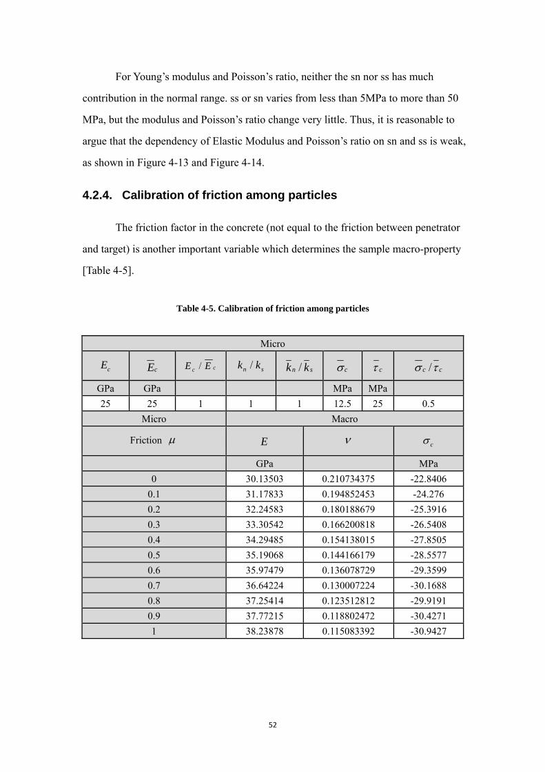
52
For Young’s modulus and Poisson’s ratio, neither the sn nor ss has much
contribution in the normal range. ss or sn varies from less than 5MPa to more than 50
MPa, but the modulus and Poisson’s ratio change very little. Thus, it is reasonable to
argue that the dependency of Elastic Modulus and Poisson’s ratio on sn and ss is weak,
as shown in Figure 4-13 and Figure 4-14.
4.2.4. Calibration of friction among particles
The friction factor in the concrete (not equal to the friction between penetrator
and target) is another important variable which determines the sample macro-property
[Table 4-5].
Table 4-5. Calibration of friction among particles
Micro
cE cE / ccE E /n sk k /n sk k cσ cτ /c cσ τ
GPa GPa MPa MPa 25 25 1 1 1 12.5 25 0.5
Micro Macro
Friction μ E ν cσ
GPa MPa 0 30.13503 0.210734375 -22.8406
0.1 31.17833 0.194852453 -24.276 0.2 32.24583 0.180188679 -25.3916 0.3 33.30542 0.166200818 -26.5408 0.4 34.29485 0.154138015 -27.8505 0.5 35.19068 0.144166179 -28.5577 0.6 35.97479 0.136078729 -29.3599 0.7 36.64224 0.130007224 -30.1688 0.8 37.25414 0.123512812 -29.9191 0.9 37.77215 0.118802472 -30.4271 1 38.23878 0.115083392 -30.9427
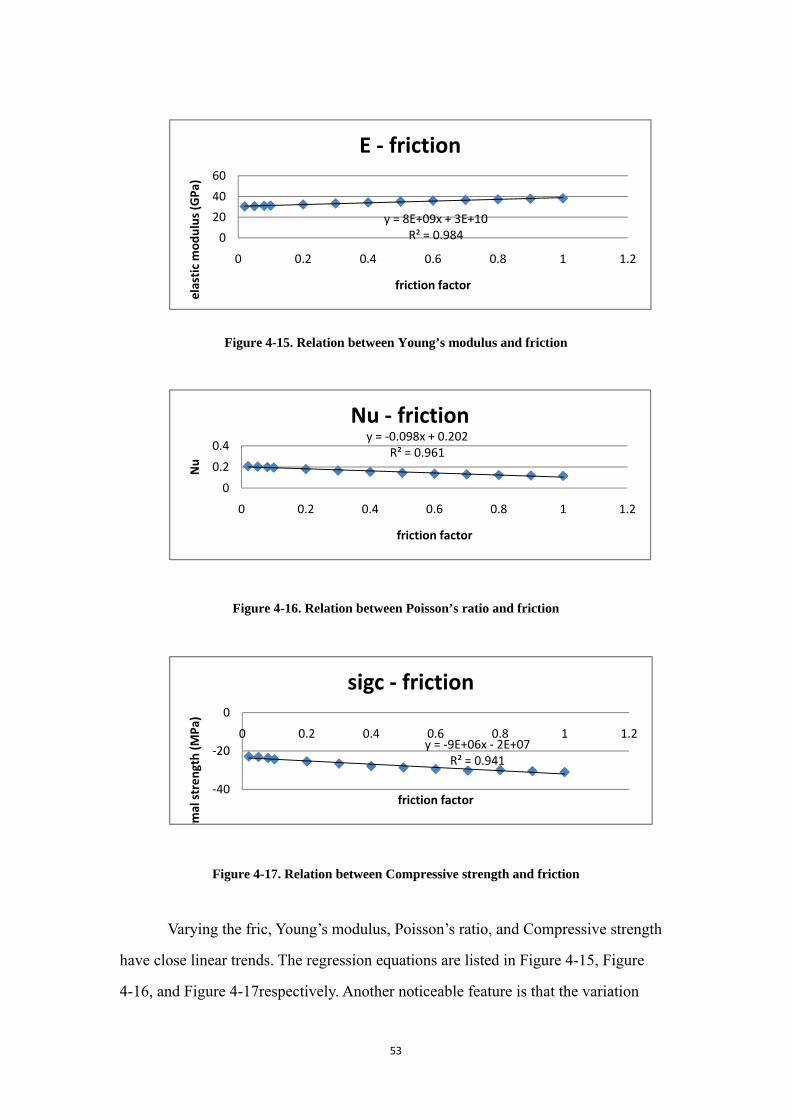
53
Figure 4-15. Relation between Young’s modulus and friction
Figure 4-16. Relation between Poisson’s ratio and friction
Figure 4-17. Relation between Compressive strength and friction
Varying the fric, Young’s modulus, Poisson’s ratio, and Compressive strength
have close linear trends. The regression equations are listed in Figure 4-15, Figure
4-16, and Figure 4-17respectively. Another noticeable feature is that the variation
y = 8E+09x + 3E+10R² = 0.9840
20
40
60
0 0.2 0.4 0.6 0.8 1 1.2
elastic mod
ulus (G
Pa)
friction factor
E ‐ friction
y = ‐0.098x + 0.202R² = 0.961
0
0.2
0.4
0 0.2 0.4 0.6 0.8 1 1.2
Nu
friction factor
Nu ‐ friction
y = ‐9E+06x ‐ 2E+07R² = 0.941
‐40
‐20
0
0 0.2 0.4 0.6 0.8 1 1.2
rmal stren
gth (M
Pa)
friction factor
sigc ‐ friction

54
ranges for three macro-parameters are not large.
9 108*10 3*10E μ= + , with R2=0.995 4-7
0.098 0.202ν μ= − + , with R2=0.961 4-8
6 79*10 2*10cσ μ= − − , with R2=0.941 4-9
Because Uniaxial Test was conducted under quasi-static loading, we dropped
out the loading velocity. Another consideration is the selection of particle size. Huang
(Huang 1999) assumed its effect is too small to be taken into account in PFC2D. We
applied the same assumption in PFC3D, while another major reason for this is
because the decrease in particle size would largely increase the calculation time,
which makes this simulation not practical for normal computer settings.
In addition to the key variables, there are other variables, like the parallel bond
radius, the standard deviation of the bond strength, etc. which also affect the sample
mechanical property. An extensive calibration test program series were conducted on
those minor variables. However, it was found that their effects on macro-properties
were either not as big as the major ones or far too irregular to do the proper analysis.
4.3. Multi-Effect Analysis and Regression Development
Based on the individual correlation between different macro-parameters and
micro-variables in the last section, those micro-variables were changed
simultaneously to investigate their combined effect. If some variables have
interdependent effect on each other, a nonlinear part would be introduced in the
regression equations.
4.3.1. Young’s Modulus
As found in the last section, Young’s modulus (E) has well-regulated

55
correlation with cE , cE , /n sk k , and μ . Therein, cE and cE can be viewed as
the direct variables affecting E, while /n sk k , and μ are the indirect ones.
Figure 4-18. Combined effects of Ec and pb_Ec on Young’s Modulus
As seen in Figure 4-18, both Ec and pb_Ec have very stable effect on E. It
seems that the effects of Ec and pb_Ec on E are independent of each other. A
regression format is provided below in order to keep the unit unification on both sides
of the equation.
( ) ( , )ncE c E E
s
kE a E b Ek
μ= + Φ 4-10
Figure 4-19. Combined effects of friction and pb_kn/ks on Young’s Modulus
As seen in Figure 4-19, both pb_kn/ks and friction have very stable effect on E.
It seems that the effects of pb_kn/ks and friction on E are independent of each other.
0
50
100
0 5 10
E (GPa
)
Ec (GPa)
E ‐ Ec
1.00E+11
1.00E+10
8.00E+08
pb_Ec
0
1
2
3
0 0.2 0.4 0.6 0.8 1
E/f(Ec,pb_
Ec)
fric
E/f(Ec,pb_Ec) ‐ fric
0.2
0.5
1
5
pb_kn/ks

56
The regression equation is proposed below.
ln nE E E
c sE c E
E kc d ea E b E k
μ= − + ++ 4-11
Use ‘Multi-linear’ regression function of EXCEL to obtain the coefficients for
different variables. The equation is listed below with the determination coefficient R2.
0.419 ln 0.386 1.0760.375 0.705
n
c sc
E kE E k
μ= − + ++
, with R2=0.929 4-12
4.3.2. Poisson’s Ratio
As found in the last section, Poisson’s ratio (ν) has well-regulated correlation
with / ccE E , /n sk k , and μ , in which /n sk k is the major variable. A regression
format is listed below for keeping the unit unification on both sides of the equation.
( , , )nc
c s
E kE kνν μ= Φ
4-13
Figure 4-20. Combined effects of friction and pb_kn/ks on Poisson’s ratio
0
0.1
0.2
0.3
0.4
0.5
0.6
0 0.2 0.4 0.6 0.8 1
Nu
u
Nu ‐ friction
0.2
0.5
1
5
pb_kn/ks

57
Figure 4-21. Combined effects of pb_kn/ks and Ec/pb_Ec on Poisson’s ratio
As seen in Figure 4-20 and Figure 4-21, both pb_kn/ks and friction have very
stable effects onν. It seems that the effects of pb_kn/ks and friction onνare
independent of each other. The similar conclusion can be drawn for pb_kn/ks and
Ec/pb_Ec.
Figure 4-22. Combined effects of Ec/pb_Ec and friction on Poisson’s ratio
However, for the correlation between friction and Ec/pb_Ec, a slight
interdependency could be found, shown in Figure 4-22. Thus, we introduce a
nonlinear term in the equation.
‐0.4
‐0.2
0
0.2
0.4
0.6
0 1 2 3 4 5 6
Nu
pb_kn/ks
Nu ‐ pb_kn/ks
0.05
0.2
1
5
Ec/pb_Ec
00.10.20.30.40.50.6
0 0.2 0.4 0.6 0.8 1
Nu
u
Nu ‐friction
0.05
0.2
1
5
Ec/pb_Ec

58
ln nc c
c cs
E Eka b c d eE k Eν ν ν ν νν μ μ= + + + +
4-14
The ‘Multi-linear’ regression function of EXCEL was used to obtain the
coefficients for different variables.
0.001 0.173ln 0.158 0.0634 0.129nc c
c cs
E EkE k E
ν μ μ= − + − + + , with R2=0.958
4-15
4.3.3. Compressive Strength
Compressive strength ( cσ ) has correlation with τ , σ , / ccE E , /n sk k ,
and μ , in which τ and σ are the major variables, with linear relationship. A
regression is provided below in order to keep unit unification on both sides of the
equation.
21
( , , )( , )
nc cc
cs
Ekk E
σ μτ σ
=ΦΦ 4-16
As stated before, the discussion of sigc was divided into into three ss/sn range:
<0.25, 0.25-4, >4. Series of tests were conducted to investigate the individual and
combined effect of different variables in these three ranges respectively.
Table 4-6. Individual effects of micro-variables on Compressive Strength
Micro- parameter Range of ss/sn Graphical correlation

59
pb_kn/ks
<0.25
0.25-4
>4
friction <0.25
y = ‐0.301x ‐ 1.093R² = 0.996
‐4
‐3
‐2
‐1
0
0 2 4 6 8
sigc/ss
pb_kn/ks
sigc/ss ‐ pb_kn/ks
y = ‐0.27ln(x) + 1.083R² = 0.993
0
0.5
1
1.5
0 2 4 6 8
sigc/f(ss,sn)
pb_kn/ks
sigc/f(ss,sn) ‐ pb_kn/ks
y = 0.644ln(x) ‐ 2.386R² = 0.972‐3
‐2
‐1
0
0 2 4 6 8
sigc/sn
pb_kn/ks
sigc/sn ‐ pb_kn/ks
y = ‐0.595x ‐ 1.012R² = 0.98
‐2
‐1.5
‐1
‐0.5
0
0 0.2 0.4 0.6 0.8 1
sigc/ss
fric
sigc/ss ‐ fric

60
0.25-4
>4
Ec/pb_Ec
<0.25
0.25-4
y = 0.203x + 0.979R² = 0.950
0.9
1
1.1
1.2
0 0.2 0.4 0.6 0.8 1
sigc/f(ss,sn)
fric
sigc/f(ss,sn) ‐ fric
y = ‐0.581x ‐ 2.115R² = 0.917
‐3
‐2
‐1
0
0 0.2 0.4 0.6 0.8 1
sigc/sn
fric
sigc/sn ‐ fric
y = ‐0.25ln(x) ‐ 1.461R² = 0.913
‐3
‐2
‐1
0
0 2 4 6 8 10
sigc/ss
Ec/pb_Ec
sigc/ss ‐ Ec/pb_Ec
y = 0.057ln(x) + 0.983R² = 0.938
0
0.5
1
1.5
0 2 4 6 8 10
sigc/f(ss,sn)
Ec/pb_Ec
sigc/f(ss,sn) ‐ Ec/pb_Ec

61
>4
As shown in Table 4-6, the sigc/f(ss,sn) have different correlation with
different micro-variables in the three ss/sn ranges. For friction, it is almost linear
relation; for Ec/pb_Ec, it is logarithmic relation; for pb_kn/ks, it has linear relation in
ss/sn<0.25, and logarithmic relation in other two ranges.
Table 4-7. Combined effects of micro-variables on Compressive Strength
Micro- parameter
Range of ss/sn Graphical correlation
pb_kn/ks &
friction <0.25
y = ‐0.24ln(x) ‐ 2.157R² = 0.940
‐3
‐2
‐1
0
0 2 4 6 8 10
sigc/sn
Ec/pb_Ec
sigc/sn ‐ Ec/pb_Ec
‐2
‐1.5
‐1
‐0.5
0
0 0.2 0.4 0.6 0.8 1
sigc/ss
fric
sigc/ss ‐ fric
0.4
1.5
5
pb_kn/ks

62
>4
Friction &
Ec/pb_Ec
<0.25
>4
Ec/pb_Ec &
pb_kn/ks <0.25
‐3
‐2
‐1
0
0 0.2 0.4 0.6 0.8 1
sigc/sn
fric
sigc/sn ‐ fric
0.4
1.5
5
pb_kn/ks
‐4
‐2
0
0 2 4 6 8 10
sigc/ss
Ec/pb_Ec
sigc/ss ‐ Ec/pb_Ec
0.05
0.2
0.9
fric
‐2
‐1.5
‐1
‐0.5
0
0 0.2 0.4 0.6 0.8 1
sigc/sn
fric
sigc/sn ‐ fric
0.04
1
8
Ec/pb_Ec
‐3
‐2
‐1
0
0 2 4 6 8 10
sigc/ss
Ec/pb_Ec
sigc/ss ‐ Ec/pb_Ec
0.4
1.5
5
pb_kn/ks

63
>4
For the range <0.25 and >4, as shown in Table 4-7, the effects of Ec/pb_Ec
and pb_kn/ks on sigc are independent of each other, so are the effects of pb_kn/ks and
fric. For the correlation in-between on fric and Ec/pb_Ec, a slight interdependency
could be found, for which a nonlinear term is introduced. And for the range 0.25-4,
Compressive strength has similar individual relation with micro-variables, but the
integral correlation becomes so complex that a good enough regression equation
wasn’t found.
Use ‘Multi-linear’ regression function of EXCEL to obtain the coefficients for
different variables. The equations for three ss/sn ranges are shown in Table 4-8 with
the determination coefficient R2.
Table 4-8. Regression equations for compressive strength
‐3
‐2
‐1
0
0 2 4 6 8 10
sigc/sn
fric
sigc/sn ‐ Ec/pb_Ec
5
1.5
5
pb_kn/ks
ss/sn range Combined Equation R2
<0.25 6 0.134 ln 0.552 0.108ln 0.176 ln ln 0.4961.3 0.5*10
nc c c
s c c
E Ekk E E
σ μ μτ
= + + + +− −
0.933
0.25-4 26 ( , , )0.752 0.249 2.2*10
nc cc
cs
Ekk E
σ μτ σ
= Φ+ −
>4 6 0.162 ln 0.061 0.013ln 0.117 ln ln 0.7742.4 1.4*10
nc c c
s c c
E Ekk E E
σ μ μσ
= − + − + +− −
0.957

64
4.3.4. Summary of the macro-micro regression equations
The empirical discoveries found above can be used to generate digital concrete
with the required mechanical properties, although the calibration still needs to be
completed step by step. The suggested procedure is in the sequence of Young’s
modulus -> Poisson’s ratio -> Compressive strength -> other parameters. Table 4-9 for
all the regression equations developed.
Table 4-9. Regression equations summary for different macro-parameters
Macro- Paramet
er
Corresponding micro-variables and regression equation with determination coefficient
E
cE cE /n sk k μ
0.419 ln 0.386 1.0760.375 0.705
n
c sc
E kE E k
μ= − + ++ , with R2=0.929
ν
/ ccE E /n sk k μ
0.001 0.173ln 0.158 0.0634 0.129nc c
c cs
E EkE k E
ν μ μ= − + − + +, with R2=0.958
cσ
ss/sn<0.25 τ μ
6 0.134 ln 0.552 0.108ln 0.176 ln ln 0.4961.3 0.5*10
nc c c
s c c
E Ekk E E
σ μ μτ
= + + + +− −
, with R2=0.98
0.25<ss/sn<4 τ and σ μ
26 ( , , )0.752 0.249 2.2*10
nc cc
cs
Ekk E
σ μτ σ
= Φ+ −
ss/sn>4 σ μ
6 0.162 ln 0.061 0.013ln 0.117 ln ln 0.772.4 1.4*10
nc c c
s c c
E Ekk E E
σ μ μσ
= − + − + +− −
, with R2=0.917

65
Chapter 5. Simulation Results and Analysis
5.1. Visualization of DEM penetration simulation
After the generation of target and projectile models, it is convenient to assign
striking velocities to the projectile and perform the impact simulation. Through
PFC3D coding, a perforation test was simulated. In the process, cracking and spalling
could be observed at the front face, while at the back face a much more significant
scabbing is the major phenomenon.
Figure 5-1. Visualization of the penetration process (with the 2nd and 3rd step enlarged)
Figure 5-1shows the concrete slab perforation process at selected time steps
(with striking velocity 500m/s). In the process, cracking and spalling could be
observed at the front face, while at the back face a much more significant scabbing is
the major phenomenon.
Different steps correspond to different times, which can be obtained from the
simulation history record, and can be used to build up the correlation with other
monitored variables, such as projectile velocity, penetration depth, friction force

66
around the projectile, etc, as shown in Figure 5-2. These correlations could be used to
analyze the mechanism of the penetration process, and compare to those from other
methods.
Figure 5-2. Visualization of the change of projectile velocity, penetration depth, and
corresponding projectile-target friction in the penetration process
Figure 5-3, Figure 5-4, and Figure 5-5 present the time history of depth,
velocity, and deceleration for a deep penetration test at impact velocity of 500 m/s,
and their comparison with empirical predictions sof the third penetration case in
(Forrestal, et al. 1994). As can be seen, the depth, velocity, and deceleration of the
projectile vary with time non-linearly. There are similar trend and range for depth and
velocity, yet the simulation has a much smaller acceleration (deceleration), which also
results in a later ending point than the real test. This could probably attribute to the
dynamic modulus property of the concrete, mentioned later.
Figure 5-3. Penetration depth of the projectile for both simulation and empirical prediction
‐0.2
0
0.2
0.4
0.6
0 0.5 1 1.5 2 2.5 3
depth (m
)
time (ms)
depth‐t
simulation
empirical
z‐ velocity (m/s)
Penetration depth (m)
Time (s)
Friction force on the projectile (N)
Time (s) Time (s)

67
Figure 5-4. Acceleration of the projectile for both simulation and empirical prediction
Figure 5-5. Velocity of the projectile for both simulation and empirical prediction
5.2. Velocity-Depth Test Validation and related factor
analysis
The velocity-penetration depth relationship is one of the important
relationships that ballistic researchers are interested in. A series of DEM simulations
with the penetration at different impact velocities into a concrete target of an
unconfined Compressive strength of 35MPa were conducted. This concrete is selected
in order to allow comparison with experimental results and empirical correlation
obtained by (Forrestal, et al. 1994).
Table 5-1 presents both the macroscopic parameters by Forrestal (1994) and
the calibrated microscopic variables obtained in this study.
‐0.4
‐0.2
0
0 0.5 1 1.5 2 2.5 3acceleration
(106m/s
2 )
time (ms)
zaccel‐t
simulation
empirical
‐500
0
500
1000
0 0.5 1 1.5 2 2.5 3
velocity (m
/s)
time (ms)
zvel‐t
simulation
empirical

68
Table 5‐2 presents the penetration depths obtained in the simulation, by the
experiments, and predicted through the empirical equation, at different impact
velocities.
Figure 5-6 also presents the data in the table graphically. It can be seen that
DEM simulation results have a similar trend as the experimental and empirical results.
However, compared to the test and Forrestal’s empirical equation, the DEM
simulation overestimates the penetration depth at lower velocities, and underestimates
the penetration depth at higher velocities. The reason is probably because the
mechanical property of concrete target is strain rate dependent, like Young’s modulus
which we would mention in the next section. And in this study only the static
properties have been calibrated.
Table 5-1. Macro-parameters and micro-variables for the test and digital concrete
Test concrete macro-parameter E(Pa) v sigc(Pa)
28.9E+9 0.167 36.2E+6
DEM micro-variable setting
rlo (m) Rratio vel_cal (m/s)5.00E-03 2 0.01 Iso_stress Tol -5.00E+04 0.1
cE (Pa) cE (Pa) / ccE E 300.0E+6 70E+9 0.0043
/n sk k /n sk k
1 3
cσ (Pa) cτ (Pa) /c cσ τ
25E+6 50E+6 0.5
Digital concrete macro-parameter E (Pa) ν cσ (Pa)
32E+9 0.17 36.9E+6
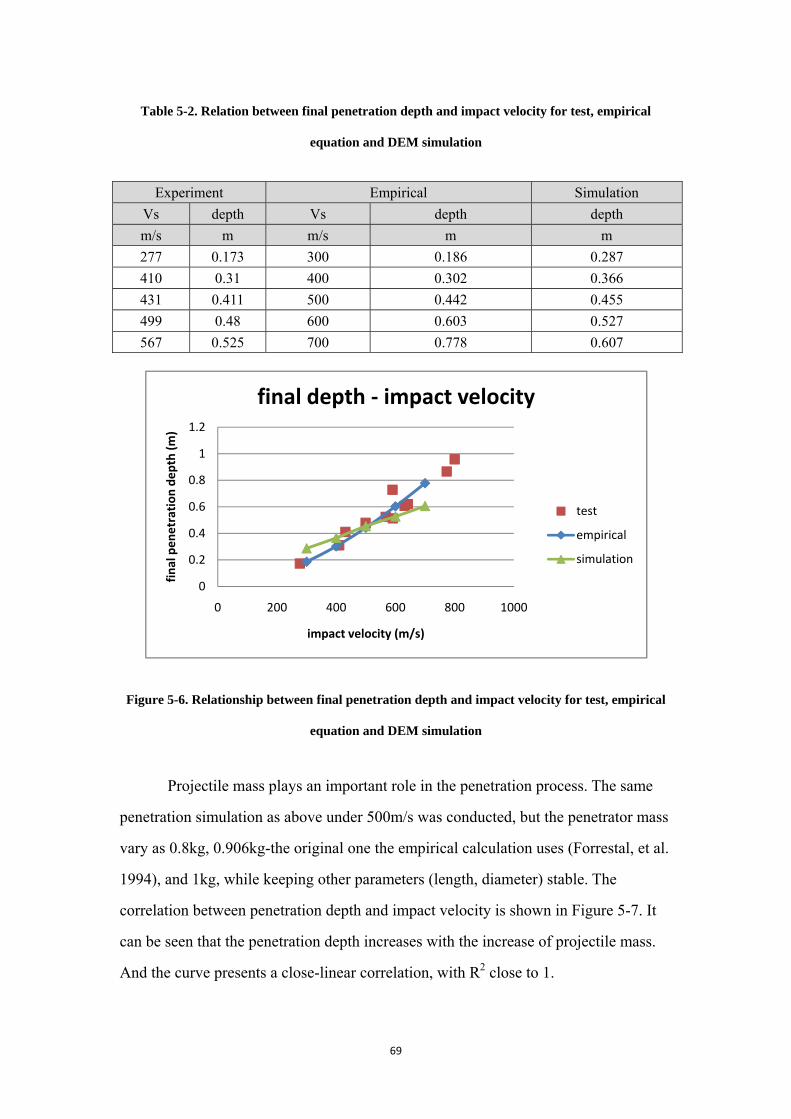
69
Table 5-2. Relation between final penetration depth and impact velocity for test, empirical
equation and DEM simulation
Experiment Empirical Simulation Vs depth Vs depth depth m/s m m/s m m 277 0.173 300 0.186 0.287 410 0.31 400 0.302 0.366 431 0.411 500 0.442 0.455 499 0.48 600 0.603 0.527 567 0.525 700 0.778 0.607
Figure 5-6. Relationship between final penetration depth and impact velocity for test, empirical
equation and DEM simulation
Projectile mass plays an important role in the penetration process. The same
penetration simulation as above under 500m/s was conducted, but the penetrator mass
vary as 0.8kg, 0.906kg-the original one the empirical calculation uses (Forrestal, et al.
1994), and 1kg, while keeping other parameters (length, diameter) stable. The
correlation between penetration depth and impact velocity is shown in Figure 5-7. It
can be seen that the penetration depth increases with the increase of projectile mass.
And the curve presents a close-linear correlation, with R2 close to 1.
0
0.2
0.4
0.6
0.8
1
1.2
0 200 400 600 800 1000
final pen
etration
dep
th (m
)
impact velocity (m/s)
final depth ‐ impact velocity
test
empirical
simulation

70
Figure 5-7. Correlation between penetration depth and projectile mass under 500m/s impact
velocity
The projectile shape is another key factor for penetration process. In this part
we make a study on the projectile tail diameter, varying the diameter as 0.02m,
0.024m, 0.028m-the original one the empirical calculation uses , 0.032m, and 0.036m,
while keeping other parameters (length, mass) stable, as shown in Figure 5-8. It can
be seen that the penetration depth decreases with the increase of projectile tail
diameter, and the curve presents a close-linear relationship, with R2 very close to 1.
Figure 5-8. Correlation between penetration depth and projectile tail diameter under impact
velocity 500m/s
As mentioned in the previous section, the interaction friction force on the
y = 0.446x + 0.045R² = 0.997
0
0.2
0.4
0.6
0.6 0.7 0.8 0.9 1 1.1 1.2
pene
tration de
pth (m
)
projectile mass (kg)
depth‐mass (500m/s)
y = ‐19.7x + 1.034R² = 0.991
0
0.2
0.4
0.6
0.8
0.015 0.02 0.025 0.03 0.035 0.04
pene
tration de
pth (m
)
projectile tail diameter (m)
depth‐tail diameter (500m/s)

71
interface of concrete and projectile is determined by *inf inf( ) vel
statf f f f e γ−= + − ,
which is set in the projectile model. However, the friction within concrete material
also plays a role in the penetration process. In the test below, we tried to make a study
on this effect. As can be seen in Figure 5-9, the bigger the friction in concrete, the
smaller the penetration depth. And this rule affects more at the higher velocity.
However, the entire variation range is not very large. The curve presents a
close-logarithmetic relationship, with R2 very close to 1.
Figure 5-9. Comparison of penetration Simulation with different friction factor
5.3. Microscopic Stress and strain relationship
In order to study the constitutive relation of concrete target under dynamic
loading, a cross section was chosen at 0.2m to study the relationship between stress
and strain, as well as strain rate. Shown in Figure 5-10, in order to minimize the
dissymmetric effect (due to the material heterogeneity), four positions at radius 0.05m
on both x-axis and y-axis are selected to find the average stress, strain, stress rate and
strain rate. The definition of stress and strain rate at a specific location (in PFC3D) is
an average over a certain volume. Thus the radius of the measurement sphere needs to
be specified, defined as 0.03m in this case. The impact velocity is 500m/s, and the
values presented are the average of the four measurements in the four spheres.
y = ‐0.04ln(x) + 0.350R² = 0.977
0
0.2
0.4
0.6
0 0.2 0.4 0.6 0.8 1 1.2
pene
tration de
pth (m
)
friction factor
depth ‐ fric (500m/s)
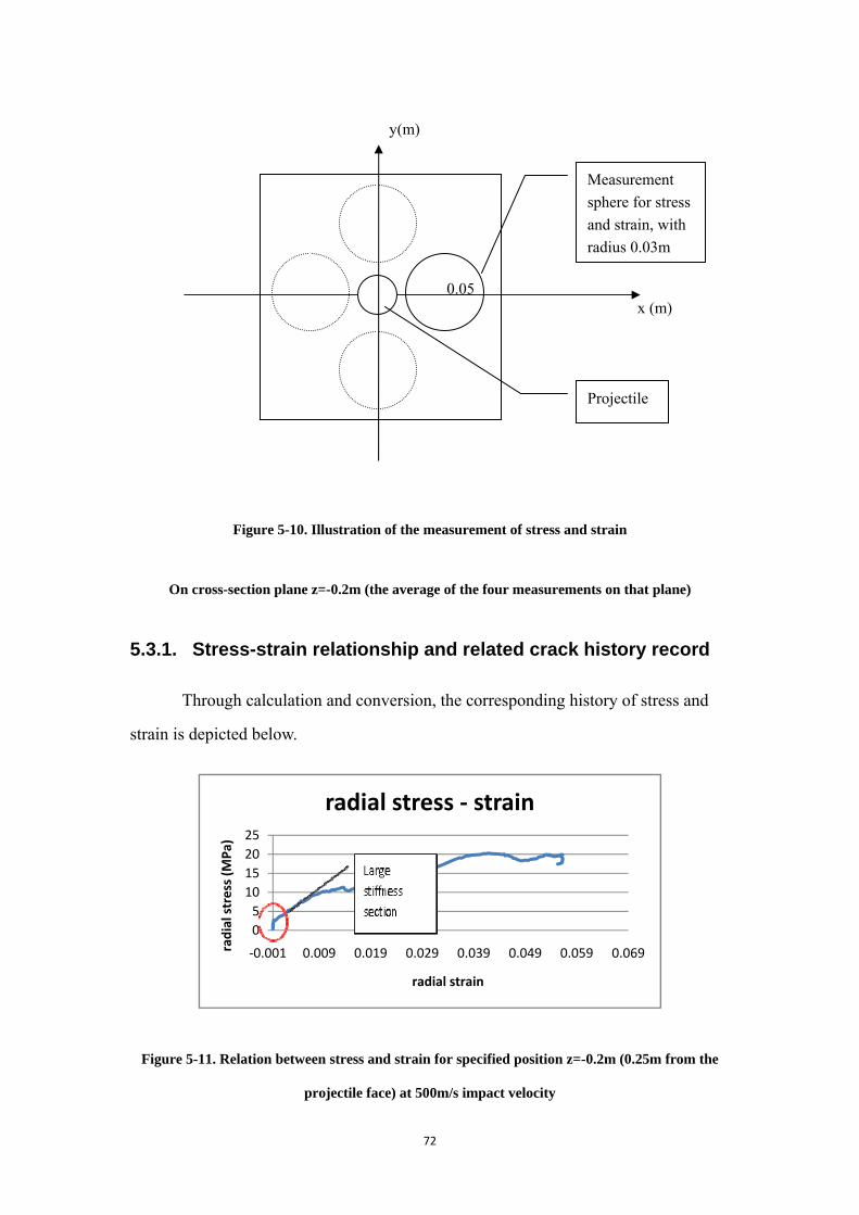
72
Figure 5-10. Illustration of the measurement of stress and strain
On cross-section plane z=-0.2m (the average of the four measurements on that plane)
5.3.1. Stress-strain relationship and related crack history record
Through calculation and conversion, the corresponding history of stress and
strain is depicted below.
Figure 5-11. Relation between stress and strain for specified position z=-0.2m (0.25m from the
projectile face) at 500m/s impact velocity
05
10152025
‐0.001 0.009 0.019 0.029 0.039 0.049 0.059 0.069radial stress (M
Pa)
radial strain
radial stress ‐ strain
Measurement sphere for stress and strain, with radius 0.03m
Projectile
y(m)
0.05 x (m)

73
Figure 5-11 presents the radial stress-radial strain relations. Its slope is related
to the elastic modulus. It can be noticed that the curve has a steep segment at first,
then the slope becomes gradually smaller (smaller modulus). The reason is probably
because the discrete contact model among particles consists of two parts (see the
methodology section): the contact-stiffness model and the parallel-bond model. The
two parts both contribute to the stiffening at first. After reaching its strength, the
parallel-bond breaks, leaving only the contribution from the contact-stiffness model.
Figure 5-12, Figure 5-13, and Figure 5-14 are the crack-radial strain and time,
penetration depth relationship, depicting the number of cracks (the break bonds) at
different radial strains. It can be seen that an instant increase in bond breakage at the
very beginning, corresponding to the stress-strain trend. It could reveal that as time
goes on, the material becomes weaker, or a time delay may exist in softening the
material. It should be noted that breakage of bonds includes the breakage of normal
bonds and shear bonds. This information is helpful in developing damage mechanics
models.
Figure 5-12. Relation between crack and radial strain at 500m/s impact velocity
‐100
900
1900
2900
3900
4900
5900
‐0.001 0.019 0.039 0.059 0.079
cracks num
ber
radial strain
crack‐radial strain
total
normal
shearLarge stiffness section

74
Figure 5-13. Relation between cracks number and time at 500m/s impact velocity
Figure 5-14. Relation between cracks number and penetration depth at 500m/s impact velocity
5.3.2. Elastic moduli – strain rate relationship analysis
To explore the relationship between the concrete modulus and strain rates, the
corresponding stress-strain, stress-time, and stress-penetration depth relationship at
impact velocities of 400m/s, 500m/s, 600m/s are plotted respectively.
‐100
1900
3900
5900
0 0.0005 0.001 0.0015 0.002 0.0025 0.003
cracks num
ber
time (s)
crack‐time
total
normal
shear
‐20
480
980
1480
‐0.002 0.048 0.098 0.148 0.198
cracks num
ber
depth (m)
crack‐depth
total
normal
shear
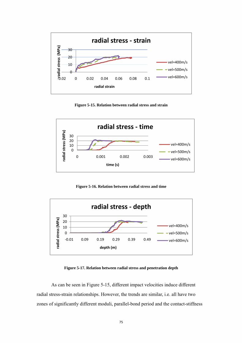
75
Figure 5-15. Relation between radial stress and strain
Figure 5-16. Relation between radial stress and time
Figure 5-17. Relation between radial stress and penetration depth
As can be seen in Figure 5-15, different impact velocities induce different
radial stress-strain relationships. However, the trends are similar, i.e. all have two
zones of significantly different moduli, parallel-bond period and the contact-stiffness
0
10
20
30
‐0.02 0 0.02 0.04 0.06 0.08 0.1radial stress (M
Pa)
radial strain
radial stress ‐ strain
vel=400m/s
vel=500m/s
vel=600m/s
0102030
0 0.001 0.002 0.003
radial stress (M
Pa)
time (s)
radial stress ‐ time
vel=400m/s
vel=500m/s
vel=600m/s
0102030
‐0.01 0.09 0.19 0.29 0.39 0.49
radial stress (M
Pa)
depth (m)
radial stress ‐ depth
vel=400m/s
vel=500m/s
vel=600m/s

76
period. This can also be reflected in Figure 5-16 and Figure 5-17, the relation between
radial stress and time and penetration depth.
Figure 5-15 also shows a general trend of the slope (the modulus) of the
stress-strain curves. It is steeper with the increase of the impact velocity. This slope
should not be considered as the static elastic modulus (obtained from calibration tests
mentioned above), but rather as the dynamic elastic modulus, which varies with strain
rates.
Table 5-3 presents the relationship between the average elastic modulus (the
ratio of stress over strain from the peak to the origin) and the maximum strain rate at
different impact velocities. Figure 5-18 presents this relationship graphically. As can
be seen, the average modulus increases with the increase of strain rate with a
non-linear relationship.
Table 5-3. Relation between average elastic modulus and strain rate, with corresponding impact
velocity and final penetration depth
velocity modulus strain rate depth m/s Pa 1/s m 400 2.54E+08 2.27E+02 0.36642 500 3.56E+08 3.11E+02 0.45483 600 3.77E+08 4.32E+02 0.52738
Figure 5-18. Relation between average elastic modulus and strain rate
0
100
200
300
400
0 100 200 300 400 500
average elastic mod
uli
(MPa
)
stain rate (1/s)
average elastic moduli ‐ strain rate

77
5.3.3. Stress distribution and time relation
In order to study the stress distribution and variation with time, several
locations along the radius direction in the target were selected for the stress plots. At
depth 0.2m, four locations at distances 0.08m, 0.05m, 0.03m, and 0.01m away from
the center of the target were selected.
For each of the four radial locations, four points, two on each of the axes, were
selected for stress averaging. (Only the locations on positive x-axis are depicted, the
other three measurement locations are on the positive y-axis, negative y-axis, and
negative x-axis. The values used below are the average results of these four locations
in order to minimize the dissymmetric effect due to the material heterogeneity.) The
stress changes with time were then observed at different penetration depths of the
projectile corresponding to different times, as shown in Figure 5-19 and Figure 5-20.
Figure 5-19. Illustration of the four measurement
locations on the cross section of the target
Figure 5-20. Illustration of the specified
measurement depth in the target (The
projectile of this illustration is not to scale)
0.1 -0.1
0.45
-0.45
x(m)
y(m)
depth0.4depth0.3depth0.2depth0.1
Measurement depth
Projectile
Projectile
y(m)
0.1
0.1
-0.1
-0.1
0.08 x (m)
0.05
0.03
0.01
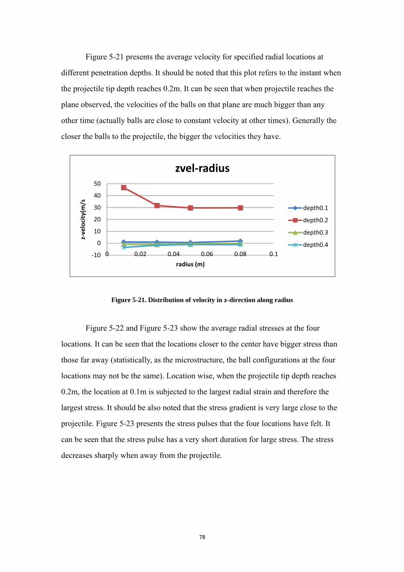
78
Figure 5-21 presents the average velocity for specified radial locations at
different penetration depths. It should be noted that this plot refers to the instant when
the projectile tip depth reaches 0.2m. It can be seen that when projectile reaches the
plane observed, the velocities of the balls on that plane are much bigger than any
other time (actually balls are close to constant velocity at other times). Generally the
closer the balls to the projectile, the bigger the velocities they have.
Figure 5-21. Distribution of velocity in z-direction along radius
Figure 5-22 and Figure 5-23 show the average radial stresses at the four
locations. It can be seen that the locations closer to the center have bigger stress than
those far away (statistically, as the microstructure, the ball configurations at the four
locations may not be the same). Location wise, when the projectile tip depth reaches
0.2m, the location at 0.1m is subjected to the largest radial strain and therefore the
largest stress. It should be also noted that the stress gradient is very large close to the
projectile. Figure 5-23 presents the stress pulses that the four locations have felt. It
can be seen that the stress pulse has a very short duration for large stress. The stress
decreases sharply when away from the projectile.
‐10
0
10
20
30
40
50
0 0.02 0.04 0.06 0.08 0.1
z‐velocity(m
/s
radius (m)
zvel‐radius
depth0.1
depth0.2
depth0.3
depth0.4
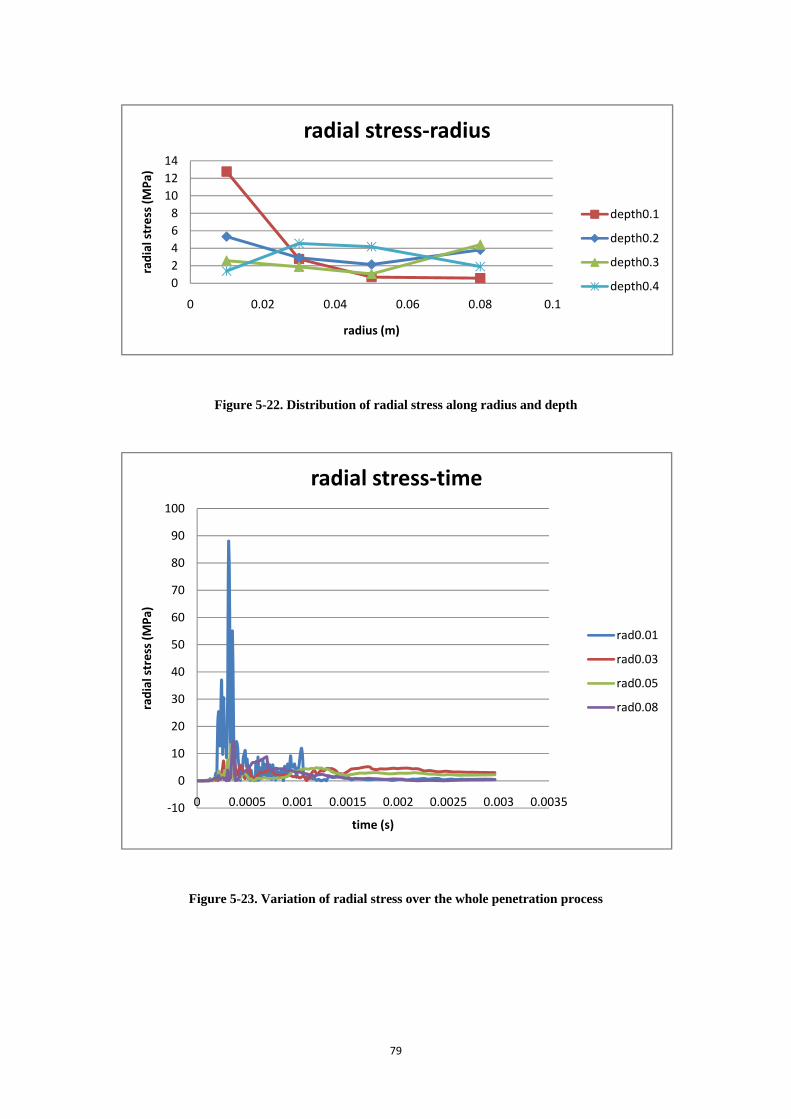
79
Figure 5-22. Distribution of radial stress along radius and depth
Figure 5-23. Variation of radial stress over the whole penetration process
02468
101214
0 0.02 0.04 0.06 0.08 0.1
radial stress (M
Pa)
radius (m)
radial stress‐radius
depth0.1
depth0.2
depth0.3
depth0.4
‐10
0
10
20
30
40
50
60
70
80
90
100
0 0.0005 0.001 0.0015 0.002 0.0025 0.003 0.0035
radial stress (M
Pa)
time (s)
radial stress‐time
rad0.01
rad0.03
rad0.05
rad0.08

80
Chapter 6. Summary and Conclusions
6.1. Scientific accomplishments
In this thesis, we applied DEM theory to build up a concrete model for
simulating the normal impact penetration process. The model and conclusions
developed in this thesis can be used for the next phase of integration of modeling,
simulation, and experimental observations.
1. An Inverse technique and digital calibration method was developed to
back-calculate the microscopic variables from the macroscopic parameters of
concrete.
2. The simulation results were compared to those obtained from experimental
and empirical methods. The Penetration Depths obtained from the simulations with
different impact velocities compare consistently with experimental and empirical
correlations.
3. The corresponding macroscopic stress – strain relations and related crack
correlations were depicted to exhibit the constitutive property. We also demonstrated
that modulus of elasticity of concrete is strain rate dependent, which can be obtained
from the average of microscopic calculations.
4. Some major parameters, like projectile mass, size, and friction factor in
concrete, were evaluated in the simulation process.
6.2. Limitation of the methodology in this thesis
The experimental equipment is still under preparation, which limits the
comparison of our simulation results to the corresponding tests.

81
PFC3D version 3.0 limits the choice of the DEM contact models, which may
not be very suitable for the concrete material. In addition, it does not have the
function of developing user-defined models like the later version.
The cluster function was not utilized in the simulation discussed in this thesis.
This creates difficulties for simulation of different sizes and irregular shapes of
aggregate.
The calculation capacity of the lab computer disables the radius of discrete
balls to further decrease, which would cause the particle number to a tremendous
amount, resulting in an unacceptable calculation time.
6.3. Recommendation for the further study
Future work is planned to incorporate the actual microstructure of concrete
into DEM simulations through x-ray computerized tomography imaging, image
analysis and using the clustering DEM.
Integration of DEM simulation into FEM simulation and use of DEM
simulation to calibrate the advanced damage mechanics models is also planned for
next phase to integrate modeling, simulation and experimental observations.

82
References
Ai‐guo, P. and H. Feng‐lei (2007). "Based on Variation Method for the Shape Optimization of
Penetrator Nose Shape."
Backman, M. E. and W. Goldsmith (1978). "Mechanics of penetration of projectiles into targets."
International Journal of Engineering Science 16(1): 1‐99.
Bernard, R. S. (1977). Empirical Analysis of Projectile Penetration in Rock. United States: 23p.
Bernard, R. S. (1978). Depth and Motion Prediction for Earth Penetrators. United States: 31p.
Bishop, R. F., R. Hill, et al. (1945). "The theory of indentation and hardness tests." Proceedings of the
Physical Society(3): 147.
Cargile, J. D. (1999). Development of a Constitutive Model for Numerical Simulation of Projectile
Penetration into Brittle Geomaterials. United States: 227p.
Chen, E. P. (1989). "Penetration into dry porous rock: a numerical study on sliding friction simulation."
Theoretical and Applied Fracture Mechanics 11(2): 135‐141.
Chen, E. P. (1994). Simulation of concrete perforation based on a continuum damage model: Size: 14
p.
Chen, X. W., S. C. Fan, et al. (2004). "Oblique and normal perforation of concrete targets by a rigid
projectile." International Journal of Impact Engineering 30(6): 617‐637.
Chen, X. W. and Q. M. Li (2002). "Deep penetration of a non‐deformable projectile with different
geometrical characteristics." International Journal of Impact Engineering 27(6): 619‐37.
Cundall, P. A. and O. D. L. Strack (1979). "Discrete numerical model for granular assemblies."
Geotechnique 29(1): 47‐65.
Forrestal, M. J. (1986). "Penetration into dry porous rock." International Journal of Solids and
Structures 22(12): 1485‐1500.
Forrestal, M. J., B. S. Altman, et al. (1994). "Empirical equation for penetration depth of ogive‐nose
projectiles into concrete targets." International Journal of Impact Engineering 15(4): 395‐405.
Forrestal, M. J., D. J. Frew, et al. (1996). "Penetration of grout and concrete targets with ogive‐nose
steel projectiles." International Journal of Impact Engineering 18(5): 465‐476.
Forrestal, M. J., D. J. Frew, et al. (2003). "Penetration of concrete targets with deceleration‐time
measurements." International Journal of Impact Engineering 28(5): 479‐497.

83
Forrestal, M. J. and D. B. Longcope (1990). "Target strength of ceramic materials for high‐velocity
penetration." Journal of Applied Physics 67(8): 3669‐3672.
Forrestal, M. J. and V. K. Luk (1988). "Dynamic spherical cavity‐expansion in a compressible
elastic‐plastic solid." Journal of Applied Mechanics, Transactions ASME 55(2): 275‐279.
Forrestal, M. J. and V. K. Luk (1992). "Penetration into soil targets." International Journal of Impact
Engineering 12(3): 427‐444.
Forrestal, M. J., K. Okajima, et al. (1988). "Penetration of 6061‐T651 aluminum targets with rigid long
rods." Journal of Applied Mechanics, Transactions ASME 55(4): 755‐760.
Forrestal, M. J. and D. Y. Tzou (1997). "Spherical cavity‐expansion penetration model for concrete
targets." International Journal of Solids and Structures 34(31‐32): 4127‐4146.
Frew, D. J., M. J. Forrestal, et al. (2001). "A split hopkinson pressure bar technique to determine
compressive stress‐strain data for rock materials." Experimental Mechanics 41(1): 40‐46.
Frew, D. J., S. J. Hanchak, et al. (1998). "Penetration of concrete targets with ogive‐nose steel rods."
International Journal of Impact Engineering 21(6): 489‐497.
Fu, Y., L. Wang, et al. (2008). "Quantification and simulation of particle kinematics and local strains in
granular materials using X‐ray tomography imaging and discrete‐element method." Journal of
Engineering Mechanics 134(2): 143‐154.
Goldsmith, W. (1999). "Non‐ideal projectile impact on targets." International Journal of Impact
Engineering 22(2‐3): 95‐395.
Gomez, J. T. and A. Shukla (2001). "Multiple impact penetration of semi‐infinite concrete."
International Journal of Impact Engineering 25(10): 965‐979.
Henderson, D. (1976). Impact and Penetration Technology Program Parametric Study. United States:
138p.
Heuze, F. E. (1990). "An overview of projectile penetration into geological materials, with emphasis on
rocks." International Journal of Rock Mechanics and Mining Science & Geomechanics
Abstracts 27(1): 1‐14.
Huang, F., H. Wu, et al. (2005). "A numerical simulation on the perforation of reinforced concrete
targets." International Journal of Impact Engineering 32(1‐4): 173‐187.
Huang, H. (1999). Discrete element modeling of tool‐rock interaction, University of Minnesota.
Doctor.
Itasca Consulting Group, I. (2005). "PFC3D (Particle Flow Code in 3 Dimensions) online Manual."
Jiao, Y., X. Zhang, et al. (2007). On using discrete particle approaches for simulating the perforation
process of concrete slab by hard projectile, Sanya, Hainan Island, China, Trans Tech

84
Publications Ltd, Stafa‐Zuerich, CH‐8712, Switzerland.
Kusano, N., T. Aoyagi, et al. (1992). "Impulsive local damage analyses of concrete structure by the
distinct element method." Nuclear Engineering and Design 138(1): 105‐110.
Li, Q. M. and X. W. Chen (2003). "Dimensionless formulae for penetration depth of concrete target
impacted by a non‐deformable projectile." International Journal of Impact Engineering 28(1):
93‐116.
Liu, K., L. Gao, et al. (2004). "Application of discrete element method in impact problems." JSME
International Journal, Series A: Solid Mechanics and Material Engineering 47(2): 138‐145.
Luk, V. K. and M. J. Forrestal (1987). "Penetration into semi‐infinite reinforced‐concrete targets with
spherical and ogival nose projectiles." International Journal of Impact Engineering 6(4):
291‐301.
Luk, V. K., M. J. Forrestal, et al. (1991). "Dynamic spherical cavity expansion of strain‐hardening
materials." Transactions of the ASME. Journal of Applied Mechanics 58(1): 1‐6.
Magnier, S. A. and F. V. Donze (1998). "Numerical simulations of impacts using a discrete element
method." Mechanics of Cohesive‐frictional Materials 3(3): 257‐276.
Ng, T.‐T. (1993). Numerical simulations for penetration process of concrete target using the discrete
element method, New Orleans, LA, USA, Publ by ASME, New York, NY, USA.
Nishida, M., K. Tanaka, et al. (2004). "Discrete element method simulation of the restitutive
characteristics of a steel spherical projectile from a particulate aggregation." JSME
International Journal, Series A (Solid Mechanics and Material Engineering) 47(3): 438‐47.
Qian, L., Y. Yang, et al. (2000). "Semi‐analytical model for truncated‐ogive‐nose projectiles penetration
into semi‐infinite concrete targets." International Journal of Impact Engineering 24(9):
947‐955.
Sawamoto, Y., H. Tsubota, et al. (1998). "Analytical studies on local damage to reinforced concrete
structures under impact loading by discrete element method." Nuclear Engineering and
Design 179(2): 157‐177.
Schoof, L. A., F. A. Maestas, et al. (1989). Numerical Method to Predict Projectile Penetration. United
States: 6p.
Tavarez, F. A. and M. E. Plesha (2004). Discrete element method for modeling penetration, San Diego,
CA, United States, American Society of Mechanical Engineers, New York, NY 10016‐5990,
United States.
Teland, J. A. and H. Sjol (2004). "Penetration into concrete by truncated projectiles." International
Journal of Impact Engineering 30(4): 447‐464.
Tham, C. Y. (2006). "Numerical and empirical approach in predicting the penetration of a concrete

85
target by an ogive‐nosed projectile." Finite Elements in Analysis and Design 42(14‐15):
1258‐1268.
W‐J.Shiu, F. Donzé, et al. (2005). "Missile impact on a concrete slab: a 3D discrete element study."
Warren, T. L. and M. R. Tabbara (1997). Spherical cavity‐expansion forcing function in PRONTO 3D for
application to penetration problems. Other Information: PBD: May 1997: Size: 27 p.
Xu, Y., L. M. Keer, et al. (1997). "Elastic‐cracked model for penetration into unreinforced concrete
targets with ogival nose projectiles." International Journal of Solids and Structures 34(12):
1479‐1491.
Young, C. W. (1967). Development of empirical equations for predicting depth of an earth‐penetrating
projectile: Pages: 40.
Young, C. W. (1972). Empirical Equations for Predicting Penetration Performance in Layered Earth
Materials for Complex Penetrator Configurations. United States: 50p.
Young, C. W. (1997). Penetration equations. United States: 37p.
Young, C. W. (1998). Simplified analytical model of penetration with lateral loading ‐‐ User's guide.
United States: 70p.
Zhang, D., F. Zhu, et al. (2005). "Application of beam‐particle model to the problem of concrete
penetration." EXPLOSION AND SHOCK WAVES 25(1).
Zhu, F. and D. Zhang (2005). "Numerical simulation of perforation in plain concrete panel with nose
shape of perforators."


![by an Explosively Formed Projectile C. Lam and D. … · Study of the Penetration of Water by an Explosively Formed Projectile C. Lam and D. McQueen DSTO-TR-0686] APPROVED FOR PUBLIC](https://img.pdfslide.us/doc/110x75/5b6b36cd7f8b9af64d8d112c/by-an-explosively-formed-projectile-c-lam-and-d-study-of-the-penetration-of.jpg)