Embed Size (px)
Citation preview
o Academy of Management Journal
1993, Vol. 36, No. 6, 1577-1613.
ON THE USE OF POLYNOMIAL REGRESSION
EQUATIONS AS AN ALTERNATIVE TO
DIFFERENCE SCORES IN
ORGANIZATIONAL RESEARCH
JEFFREY R. EDWARDS
University of Michigan
MARK E. PARRY
University of Virginia
For decades, difference scores have been widely used in studies of con-
gruence in organizational research. Although methodological problems with difference scores are well known, few viable alternatives have
been proposed. One alternative involves the use of polynomial regres- sion equations, which permit direct tests of the relationships difference
scores are intended to represent. Unfortunately, coefficients from poly- nomial regression equations are often difficult to interpret. We used
response surface methodology to develop an interpretive framework
and illustrate it using data from a well-known person-environment
study. Several important findings not reported in the original study
emerged.
For decades, difference scores have been widely used in both micro and
macro organizational research. Typically, these scores have consisted of the
algebraic, absolute, or squared difference between two component measures
(e.g., Alexander & Randolph, 1985; Dougherty & Pritchard, 1985; French,
Caplan, & Harrison, 1982; Rice, McFarlin, & Bennett, 1989; Tubbs & Dahl,
1991; Turban & Jones, 1988) or the sum of absolute or squared differences
between profiles of component measures (e.g., Drazin & Van de Ven, 1985;
Gresov, 1989; Rounds, Dawis, & Lofquist, 1987; Sparrow, 1989; Turban &
Jones, 1988; Vancouver & Schmitt, 1991; Venkatraman, 1990; Venkatraman
& Prescott, 1990; Zalesny & Kirsch, 1989). In most cases, difference scores are
used to represent congruence (i.e., fit, match, similarity, or agreement) be-
tween two constructs, which is then viewed as a predictor of some outcome
(Edwards, 1991; Mowday, 1987; Wanous, Poland, Premack, & Davis, 1992; Van de Ven & Drazin, 1985).
Support for this research was provided in part by contract #HSM-99-72-61 from the Na-
tional Institute of Occupational Safety and Health, the Institute for Social Research at the
University of Michigan, and the Darden Graduate Business School Foundation at the University of Virginia. We thank Shyamal Peddada and Donald Richards for their technical advice and R.
Van Harrison for his assistance in obtaining the data.
1577
This content downloaded from 152.2.176.242 on Wed, 03 Feb 2016 18:33:43 UTCAll use subject to JSTOR Terms and Conditions
Academy of Management Journal
As is widely known, difference scores suffer from numerous substantive
and methodological problems (Cronbach & Furby, 1970; Edwards, in press;
Johns, 1981). An alternative procedure involves the use of polynomial re-
gression equations containing the component measures composing the dif-
ference and certain higher-order terms, such as the squares of both compo- nent measures and their product (Edwards, in press). These equations per- mit a researcher to avoid many problems associated with difference scores
but nonetheless obtain direct tests of conceptual models relevant to the
study of congruence. Despite their advantages, polynomial equations often
yield results that are difficult to interpret, particularly when their coeffi-
cients deviate from patterns corresponding to difference scores, as is usually the case (Edwards, 1992, in press; Edwards & Harrison, 1993). These inter-
pretive difficulties are likely to prevent the widespread use of polynomial
regression equations in the study of congruence, even though their use over-
comes longstanding problems with difference scores.
This article provides a systematic framework for testing and interpreting
polynomial regression equations within the study of congruence in organ- izational research. This framework draws from response surface methodol-
ogy (Box & Draper, 1987; Khuri & Cornell, 1987), which permits precise
description and evaluation of three-dimensional surfaces corresponding to
polynomial regression equations. We illustrate the application of the frame-
work using data from the classic study of person-environment (P-E) fit by French, Caplan, and Harrison (1982).
POLYNOMIAL REGRESSION AS AN ALTERNATIVE TO
DIFFERENCE SCORES
Edwards (1991, in press; Edwards & Cooper, 1990) has described the
polynomial regression procedure, showing how polynomial regression equa- tions avoid problems with difference scores but permit direct tests of the
relationships difference scores are intended to represent. This is illustrated
by the following regression equation, which uses an algebraic difference as
a single predictor (e.g., French et al., 1982; Kernan & Lord, 1990; Vance &
Colella, 1990; Wanous & Lawler, 1972):
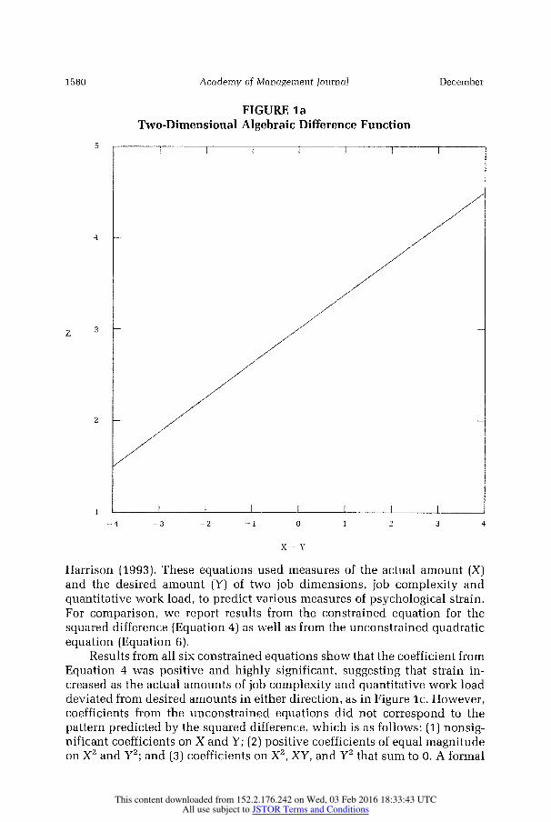
Z = bo + b(X - Y) + e. (1)
In this equation, X and Y represent the two component measures comprising the difference, Z represents an outcome measure, and e represents a random
disturbance term. The positive sign on b1 indicates that the difference be-
tween X and Y is positively related to Z (see Figure la). Expanding this
equation yields:
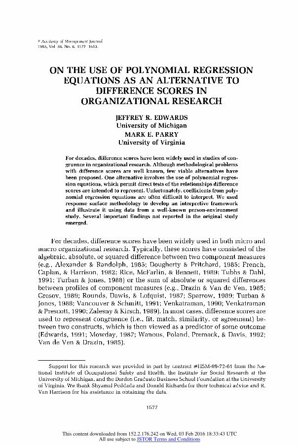
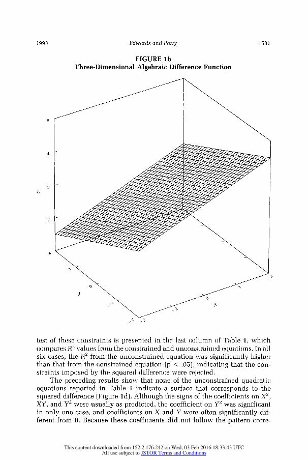
Z = bo + b1X - b1Y + e. (2)
This expansion shows that Equation 1 implies a positive relationship be-
tween X and Z and a negative relationship between Y and Z (Figure lb), with
the constraint that the coefficients on X and Y are equal in magnitude but
December 1578
This content downloaded from 152.2.176.242 on Wed, 03 Feb 2016 18:33:43 UTCAll use subject to JSTOR Terms and Conditions
Edwards and Parry
opposite in sign. The following equation relaxes this constraint, allowing the
coefficients on X and Y to take on whatever values maximize the variance
explained in Z:
Z = bo + b1X + b2Y + e. (3)
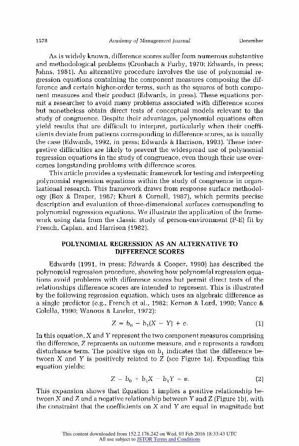
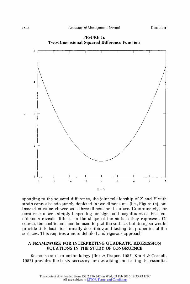
A somewhat more complicated equation uses the squared difference
between two component measures (e.g., Caplan, Cobb, French, Harrison, &
Pinneau, 1980; Dougherty & Pritchard, 1985; Tsui & O'Reilly, 1989):
Z = bo + bl(X -
)2 + e. (4)
The positive sign on b1 indicates that Z increases as the difference between
X and Y increases in either direction (Figure lc). Expanding this equation
yields:
Z = bo + blX2
- 2biXY + b1Y2 + e. (5)
This equation shows that a squared difference implies positive coefficients
of equal magnitude on X2 and Y2 along with a negative coefficient twice as
large in absolute magnitude on XY (Figure 1d). This equation also shows that
Equation 4 implicitly contains curvilinear and interactive terms without
appropriate lower-order terms (Cohen, 1978). Relaxing the constraints in
Equation 5 and adding lower-order terms yields:
Z = bo + b1X + b2Y + b3X2 + b4XY + b5Y2 + e. (6)
This equation shows that a squared difference imposes four constraints: (1) The coefficient on X is 0, (2) the coefficient on Y is 0, (3) the coefficients on
X2 and y2 are equal, and (4) the coefficients on X2, XY, and Y2 sum to 0;
given the third constraint, this is equivalent to stating that the coefficient on
XY is twice as large as the coefficient on either X2 or Y2, but opposite in sign (cf. Edwards, in press). As will be shown later, Equation 6 can be used to test
these constraints as well as to depict surfaces substantially more complex than that corresponding to the squared difference (Figure ld).
Studies using the polynomial regression procedure (Edwards, 1992, in
press; Edwards & Harrison, 1993) have yielded two general findings. First, most relationships of interest can be depicted using either a linear or a
quadratic equation (Equations 3 and 6, respectively). Second, the constraints
difference scores impose on these equations are usually rejected, making it
necessary to interpret coefficients from the unconstrained linear and qua- dratic equations. Although interpreting coefficients from linear equations is
relatively straightforward, coefficients from quadratic equations are often
difficult to interpret, particularly when they deviate from the pattern im-
plied by the squared difference (see Equation 5), as is usually the case.
Unfortunately, studies using the polynomial regression procedure have of-
fered little guidance for interpreting coefficients from quadratic equations when the constraints imposed by the squared difference are rejected.
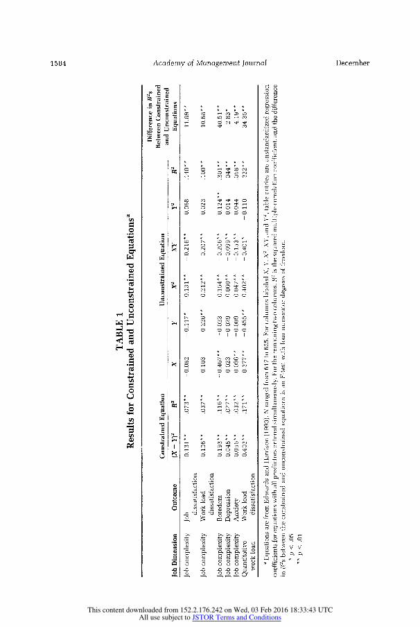
To illustrate the difficulty of interpreting coefficients from quadratic
regression equations, Table 1 reports six equations analyzed by Edwards and
1993 1579
This content downloaded from 152.2.176.242 on Wed, 03 Feb 2016 18:33:43 UTCAll use subject to JSTOR Terms and Conditions
Academy of Management Journal
FIGURE la
Two-Dimensional Algebraic Difference Function
5
4
z 3
2
-4 -3 -2 -1 0 1 2 3 4
X-Y
Harrison (1993). These equations used measures of the actual amount (X) and the desired amount (Y) of two job dimensions, job complexity and
quantitative work load, to predict various measures of psychological strain.
For comparison, we report results from the constrained equation for the
squared difference (Equation 4) as well as from the unconstrained quadratic
equation (Equation 6). Results from all six constrained equations show that the coefficient from
Equation 4 was positive and highly significant, suggesting that strain in-
creased as the actual amounts of job complexity and quantitative work load
deviated from desired amounts in either direction, as in Figure lc. However, coefficients from the unconstrained equations did not correspond to the
pattern predicted by the squared difference, which is as follows: (1) nonsig- nificant coefficients on X and Y; (2) positive coefficients of equal magnitude on X2 and Y2; and (3) coefficients on X2, XY, and y2 that sum to 0. A formal
December 1580
This content downloaded from 152.2.176.242 on Wed, 03 Feb 2016 18:33:43 UTCAll use subject to JSTOR Terms and Conditions
Edwards and Parry
FIGURE lb
Three-Dimensional Algebraic Difference Function
5
4
z
'V
test of these constraints is presented in the last column of Table 1, which
compares R2 values from the constrained and unconstrained equations. In all
six cases, the R2 from the unconstrained equation was significantly higher than that from the constrained equation (p < .05), indicating that the con-
straints imposed by the squared difference were rejected. The preceding results show that none of the unconstrained quadratic
equations reported in Table 1 indicate a surface that corresponds to the
squared difference (Figure ld). Although the signs of the coefficients on X2,
XY, and Y2 were usually as predicted, the coefficient on y2 was significant in only one case, and coefficients on X and Y were often significantly dif-
ferent from 0. Because these coefficients did not follow the pattern corre-
1993 1581
This content downloaded from 152.2.176.242 on Wed, 03 Feb 2016 18:33:43 UTCAll use subject to JSTOR Terms and Conditions
Academy of Management Journal
FIGURE lc
Two-Dimensional Squared Difference Function
5
4
Z 3
-4 -3 -2 -1 0 1 2 3
X-Y
sponding to the squared difference, the joint relationship of X and Y with
strain cannot be adequately depicted in two dimensions (i.e., Figure Ic), but
instead must be viewed as a three-dimensional surface. Unfortunately, for
most researchers, simply inspecting the signs and magnitudes of these co-
efficients reveals little as to the shape of the surface they represent. Of
course, the coefficients can be used to plot the surface, but doing so would
provide little basis for formally describing and testing the properties of the
surfaces. This requires a more detailed and rigorous approach.
A FRAMEWORK FOR INTERPRETING QUADRATIC REGRESSION
EQUATIONS IN THE STUDY OF CONGRUENCE
Response surface methodology (Box & Draper, 1987; Khuri & Cornell,
1987) provides the basis necessary for describing and testing the essential
December 1582
This content downloaded from 152.2.176.242 on Wed, 03 Feb 2016 18:33:43 UTCAll use subject to JSTOR Terms and Conditions
Edwards and Parry
FIGURE ld
Three-Dimensional Squared Difference Function
5
z
2
features of surfaces corresponding to quadratic regression equations. We
focused on three key features of these surfaces. The first is the stationary
point (i.e., the point at which the slope of the surface is 0 in all directions), which corresponds to the overall minimum, maximum, or saddle point of
the surface. The second feature is the principal axes of the surface, which
run perpendicular to one another and intersect at the stationary point. For
convex surfaces,1 the upward curvature is greatest along the first principal
1 A quadratic surface is convex if a line connecting any two points on the surface lies on or
above that surface, whereas a quadratic surface is concave if a line connecting any two points on the surface lies on or below that surface (Chiang, 1974: 255).
1993 1583
I , ,,
This content downloaded from 152.2.176.242 on Wed, 03 Feb 2016 18:33:43 UTCAll use subject to JSTOR Terms and Conditions
01
4^>
TABLE 1
Results for Constrained and Unconstrained Equationsa
Difference in R2s
Between Constrained ^ Constrained Equation Unconstrained Equationonstr d
and Unconstrained CL
Job Dimension Outcome (X - Y)2 R2 X Y X2 XY y2 R2 Equations
Job complexity Job 0.131** .073** -0.082 -0.117* 0.131** -0.216** 0.068 .140** 11.89**
dissatisfaction
Job complexity Work load 0.108** .037** 0.103 -0.226** 0.212** -0.207** 0.023 .100** 10.68*
dissatisfaction
Job complexity Boredom 0.193** .116** -0.467** -0.023 0.154** -0.206** 0.124** .301** 40.51**
Job complexity Depression 0.048** .027** 0.023 -0.029 0.060** -0.099** 0.014 .044** 2.83*
Job complexity Anxiety 0.056** .032** 0.096** -0.009 0.047** -0.153** 0.044 .058** 4.19**
Quantitative Work load 0.402** .171** 0.377** -0.455** 0.402** -0.401* -0.110 .322** 34.35**
work load dissatisfaction
a Equations are from Edwards and Harrison (1993). N ranged from 617 to 625. For columns labeled X, Y, X2, XY, and Y2, table entries are unstandardized regression k
coefficients for equations with all predictors entered simultaneously. For the remaining two columns, R2 is the squared multiple correlation coefficient, and the difference
in R2s between the constrained and unconstrained equations is an F-test with four numerator degrees of freedom. *
p < .05
**p < .01
CD
nc
This content downloaded from 152.2.176.242 on Wed, 03 Feb 2016 18:33:43 UTCAll use subject to JSTOR Terms and Conditions
Edwards and Parry
axis and least along the second principal axis. For concave surfaces, the
downward curvature is least along the first principal axis and greatest along the second principal axis. For saddle-shaped surfaces, the upward curvature
is greatest along the first principal axis, and the downward curvature is
greatest along the second principal axis. Finally, the third feature is the slope of the surface along various lines of interest, such as the principal axes and
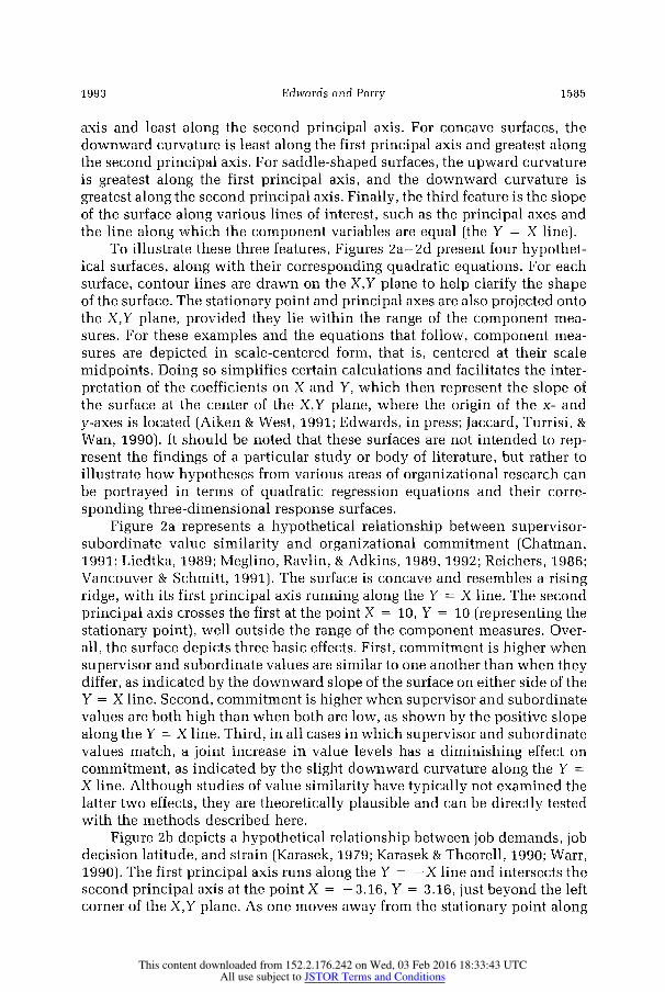
the line along which the component variables are equal (the Y = X line). To illustrate these three features, Figures 2a-2d present four hypothet-
ical surfaces, along with their corresponding quadratic equations. For each
surface, contour lines are drawn on the X,Y plane to help clarify the shape of the surface. The stationary point and principal axes are also projected onto
the X,Y plane, provided they lie within the range of the component mea-
sures. For these examples and the equations that follow, component mea-
sures are depicted in scale-centered form, that is, centered at their scale
midpoints. Doing so simplifies certain calculations and facilitates the inter-
pretation of the coefficients on X and Y, which then represent the slope of
the surface at the center of the X,Y plane, where the origin of the x- and
y-axes is located (Aiken & West, 1991; Edwards, in press; Jaccard, Turrisi, &
Wan, 1990). It should be noted that these surfaces are not intended to rep- resent the findings of a particular study or body of literature, but rather to
illustrate how hypotheses from various areas of organizational research can
be portrayed in terms of quadratic regression equations and their corre-
sponding three-dimensional response surfaces.
Figure 2a represents a hypothetical relationship between supervisor- subordinate value similarity and organizational commitment (Chatman, 1991; Liedtka, 1989; Meglino, Ravlin, & Adkins, 1989, 1992; Reichers, 1986; Vancouver & Schmitt, 1991). The surface is concave and resembles a rising
ridge, with its first principal axis running along the Y = X line. The second
principal axis crosses the first at the point X = 10, Y = 10 (representing the
stationary point), well outside the range of the component measures. Over-
all, the surface depicts three basic effects. First, commitment is higher when
supervisor and subordinate values are similar to one another than when they differ, as indicated by the downward slope of the surface on either side of the
Y = X line. Second, commitment is higher when supervisor and subordinate
values are both high than when both are low, as shown by the positive slope
along the Y = X line. Third, in all cases in which supervisor and subordinate
values match, a joint increase in value levels has a diminishing effect on
commitment, as indicated by the slight downward curvature along the Y =
X line. Although studies of value similarity have typically not examined the
latter two effects, they are theoretically plausible and can be directly tested
with the methods described here.
Figure 2b depicts a hypothetical relationship between job demands, job decision latitude, and strain (Karasek, 1979; Karasek & Theorell, 1990; Warr,
1990). The first principal axis runs along the Y = -X line and intersects the
second principal axis at the point X = - 3.16, Y = 3.16, just beyond the left
corner of the X,Y plane. As one moves away from the stationary point along
1993 1585
This content downloaded from 152.2.176.242 on Wed, 03 Feb 2016 18:33:43 UTCAll use subject to JSTOR Terms and Conditions
Academy of Management Journal
FIGURE 2aa
Hypothetical Surface for Supervisor and Subordinate
Values Predicting Organizational Commitment
(Z = 5 + .1X + .1Y- .05X2 + .09XY- .05Y2)
5
4 z
N-N
o 3
H -
a On the X,Y plane, the dotted line running diagonally from the near corner to the far corner
represents the Y = X line, and the dotted line running diagonally left to right represents the
Y = -X line. When the principal axes cross the X,Y plane within the range of the X and Y
measure, the first principal axis is represented by a solid line and the second principal axis is
represented by a dashed line.
December 1586
This content downloaded from 152.2.176.242 on Wed, 03 Feb 2016 18:33:43 UTCAll use subject to JSTOR Terms and Conditions

Edwards and Parry
FIGURE 2ba
Hypothetical Surface for Job Demand and Job Decision Latitude
Predicting Strain (Z = 3 + .3X - .3Y + .025X2 - .045XY + .025Y2)
6
4
3 N-
c-r CC d r-
3
, l
3
a On the X,Y plane, the dotted line running diagonally from the near corner to the far corner
represents the Y = X line, and the dotted line running diagonally left to right represents the
Y = -X line. When the principal axes cross the X,Y plane within the range of the X and Y
measure, the first principal axis is represented by a solid line and the second principal axis is
represented by a dashed line.
1993 1587
This content downloaded from 152.2.176.242 on Wed, 03 Feb 2016 18:33:43 UTCAll use subject to JSTOR Terms and Conditions
Academy of Management Journal
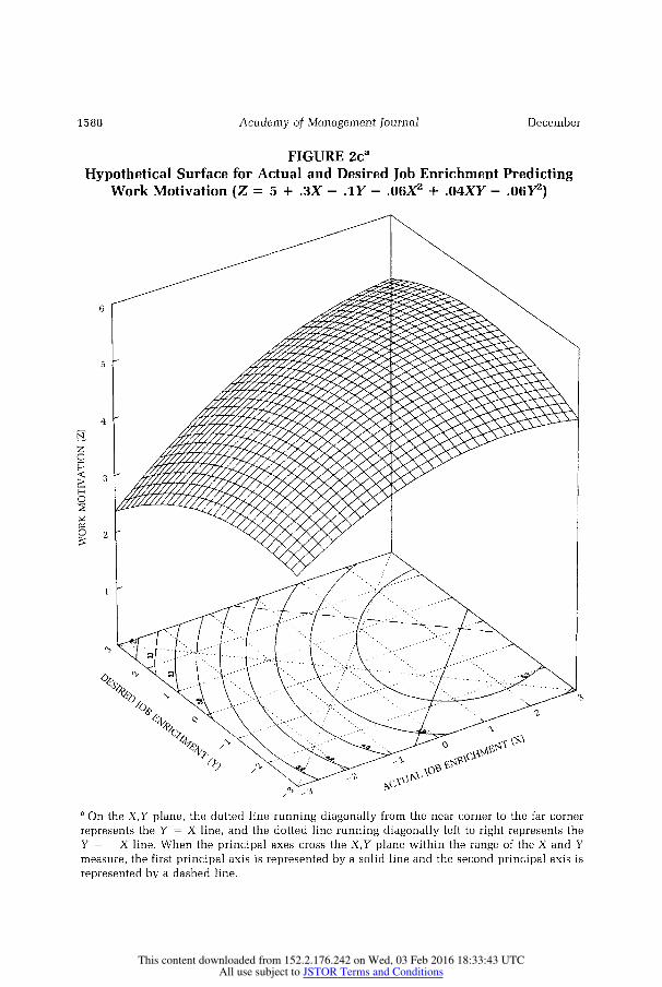
FIGURE 2ca
Hypothetical Surface for Actual and Desired Job Enrichment Predicting Work Motivation (Z = 5 + .3X - .1Y- .06X2 + .04XY - .06Y2)
6
5 '
4
a On the X,Y plane, the dotted line running diagonally from the near corner to the far corner
represents the Y = X line, and the dotted line running diagonally left to right represents the
Y = -X line. When the principal axes cross the X,Y plane within the range of the X and Y
measure, the first principal axis is represented by a solid line and the second principal axis is
represented by a dashed line.
December 1588
This content downloaded from 152.2.176.242 on Wed, 03 Feb 2016 18:33:43 UTCAll use subject to JSTOR Terms and Conditions
Edwards and Parry
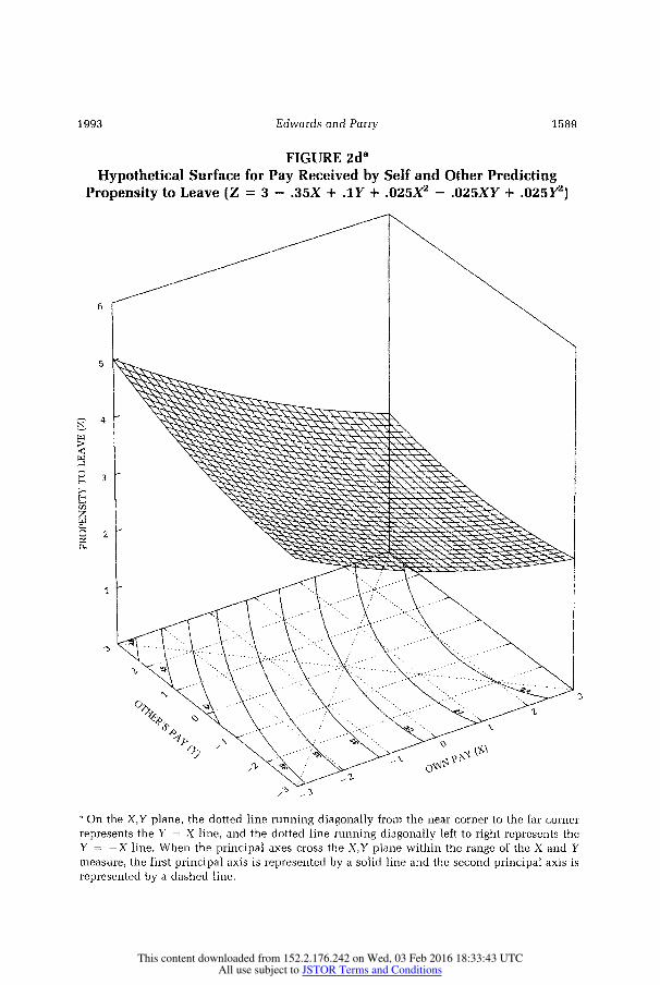
FIGURE 2da
Hypothetical Surface for Pay Received by Self and Other Predicting
Propensity to Leave (Z = 3 - .35X + .1Y + .025X2 - .025XY + .025Y2)
6
0 2~'
1
a On the X,Y plane, the dotted line running diagonally from the near corner to the far corner
represents the Y - X line, and the dotted line running diagonally left to right represents the
Y = -X line. When the principal axes cross the X,Y plane within the range of the X and Y
measure, the first principal axis is represented by a solid line and the second principal axis is
represented by a dashed line.
1993 1589
This content downloaded from 152.2.176.242 on Wed, 03 Feb 2016 18:33:43 UTCAll use subject to JSTOR Terms and Conditions
Academy of Management Journal
the first principal axis, the surface is positively sloped and somewhat con-
vex. In essence, the surface indicates that strain is lowest when job demands
are low and job decision latitude is high but increases at an increasing rate
as job demands increase and job decision latitude decreases. The surface
also indicates that strain is essentially constant when job demands match job decision latitude, as shown by the minimal slope along the Y = X line.
Figure 2c shows a hypothetical relationship between actual job enrich-
ment, desired job enrichment, and work motivation (Cherrington & England, 1980; Hackman & Oldham, 1980; Kulik, Oldham, & Hackman, 1987). The
surface is concave and slightly elliptical, with its first principal axis running
parallel to the Y = X line but displaced to the right, into the region where X
is greater than Y. The second principal axis intersects the first at the point X = 2.5, Y = 0, just inside the right edge of the X,Y plane. Overall, the surface
indicates three effects. First, motivation increases as actual enrichment in-
creases toward desired enrichment but begins to decrease when actual en-
richment has moderately exceeded desired enrichment (in this case, by 2.5
units). Second, motivation is generally higher when actual and desired en-
richment are high than when both are low. Third, when actual and desired
enrichment are both high (in this case, about 1.25 units), motivation begins to decrease, suggesting that intense involvement may eventually lead to poor mental health, burnout, and other conditions deleterious to motivation (Ku- lik et al., 1987).
Finally, Figure 2d depicts the hypothetical effects of the pay received by oneself and a referent other on one's propensity to leave (Dittrich & Carrell,
1979; Oldham, Kulik, Ambrose, Stepina, & Brand, 1986; Scholl, Cooper, &
McKenna, 1987; Summers & Hendrix, 1991; Telly, French, & Scott, 1971). The surface is convex, with its first principal axis running parallel to the Y
= -X line but intersecting the second principal axis at the point X = 8, Y
2, well outside of the X,Y plane. As one moves along the Y = X line, the
surface is sloped downward and slightly convex. Overall, the surface indi-
cates three effects. First, propensity to leave is notably greater for conditions
of underpayment than for conditions of overpayment. Second, when the pay received by oneself and a referent other both increase equally, one's propen-
sity to leave decreases. Third, as one moves up the pay scale, successively
larger increases in pay received by both parties are required to produce a unit
decrease in propensity to leave.
Ideally, the preceding examples would have been based on results from
empirical studies of congruence that examined three-dimensional surfaces.
Unfortunately, most studies of congruence have focused on two-
dimensional relationships. That focus compelled us to derive plausible hy-
potheses from the literature to illustrate how relationships of interest in
organizational research can be meaningfully depicted in terms of quadratic
regression equations and their associated response surfaces. These surfaces
show not only the effects of congruence between the component measures, but also other substantively meaningful effects, such as slope and curvature
along the principal axes and the Y = X line, shifts in surface maxima or
1590 December
This content downloaded from 152.2.176.242 on Wed, 03 Feb 2016 18:33:43 UTCAll use subject to JSTOR Terms and Conditions
Edwards and Parry
minima away from the Y = X line, and so on. These examples also show that
the location of the stationary point and principal axes and the slope of the
surface along various lines of interest provide the core information necessary to interpret most surfaces. Fortunately, these features can be readily calcu-
lated from coefficients obtained from quadratic regression equations, as
shown below.
Locating the Stationary Point and Principal Axes
Formulas expressing the stationary point and principal axes in terms of
regression coefficients were derived from equations reported by Khuri and
Cornell (1987). For a quadratic regression equation, the X,Y coordinates of
the stationary point (Xo, Yo) are:
b2b4 - 2bib5 Xo0= 4b b25 (7)
4b3b5 - b4
and
_ bb4 - 2b2b3
Yo 4b3b5 - b 2
Note that when the equality 4b3b5 = b2 holds, Equations 7 and 8 are unde-
fined, meaning that the surface has no stationary point. This condition im-
plies one of two types of surface, depending on the values of b3, b4, and b5. If any of these coefficients is nonzero, the surface is either a ridge with a
constant slope along its first principal axis or a trough with a constant slope
along its second principal axis. If b3, b4, and b5 equal 0 simultaneously, the
surface is a plane (e.g., Figure lb). In this case, the interpretation of the
surface is straightforward and does not require the framework described
here.
The first and second principal axes can be expressed as lines in the X,Y
plane. The equation for the first principal axis can be written as
Y = Plo + P1X. (9)
The equation for p11 is
b5 - b3 + (b3 - b5)2 + b
Pii b (10) P4
Two properties of Equation 10 are worth noting. First, when b3 and b5 are
equal (as implied by the squared difference), Equation 10 reduces to Ib4j/b4. In this case, p11 equals either 1 or - 1, depending upon whether the sign of
b4 is positive or negative. Second, when b4 equals 0, both the numerator and
denominator of Equation 10 become 0, rendering it undefined. In that case, one of three implications regarding the first principal axis of the surface
pertains: if b3 is greater than b5, the first principal axis has a slope of 0 and
runs parallel to the x-axis. If b3 is less than b5, the first principal axis has a
1993 1591
This content downloaded from 152.2.176.242 on Wed, 03 Feb 2016 18:33:43 UTCAll use subject to JSTOR Terms and Conditions
Academy of Management Journal
slope of infinity and runs parallel to the y-axis. Finally, if b3 and b5 are equal, the surface is a symmetric bowl or cap (depending on whether b3 and b5 are
positive or negative), and no unique set of axes can be identified.
Once X0, Yo, and p,1 have been calculated, P1o can be calculated using the following formula:
Pio Yo - P11X (11)
Note that if Pll equals 0, P1o equals Yo, indicating that the first principal axis
runs parallel to the x-axis and intersects the y-axis at the point Yo. The equation for the second principal axis can be written as
Y = P20 + P21X. (12)
The equation for P21 is
b5 - b3 - \/(b3 - b)2 + b2 P21 b4 (13)
Note that the equation for p21 is identical to that for Pll, except that the
sign preceding the expression the expression /(b3 - b5)2 + b4 is reversed.
Hence, when b3 and b5 are equal, Equation 13 becomes equivalent to
-Ib4l/b4. Consequently, if b4 is positive, P21 equals -1, whereas if b4 is
negative, P21 equals 1. Analogously, if b4 equals 0 and b3 is greater than b5, the slope of the second principal axis is infinity, whereas if b4 equals 0 and
b3 is less than b5, the slope of the second principal axis is 0. As before, if b4
equals 0 and b3 and b5 are equal, the surface has no unique set of principal axes.
Once Xo, Yo, and P21 have been calculated, P20 can be calculated as
follows:
P2o = Yo - p21Xo. (14)
The preceding equations can be used to locate the principal axes in
reference to the x- and y-axes. However, other information regarding the
location of the principal axes may also be relevant. For example, congruence researchers often hypothesize that some outcome, such as job satisfaction or
company performance, is maximized at the point of "perfect fit" (e.g., Drazin
& Van de Ven, 1985; Rice et al., 1989). This hypothesis implies a ridge with
its first principal axis running along the Y = X line, meaning that Pio = 0
and Pii = 1. If P11 differs from 1, the surface is rotated off the Y = X line.
If the quantity -plo/(l + P11) differs from 0, the surface is shifted laterally
along the Y = -X line, with its first principal axis intersecting that line at
the point X = -po/(l + P11), Y = plo/(l + Pl). In either case, the hy-
pothesis that the first principal axis runs along the Y = X line is rejected.
Congruence researchers also hypothesize that certain outcomes, such as
psychological strain and turnover, are minimized at the point of perfect fit
(e.g., Dittrich & Carrell, 1979; French et al., 1982). This hypothesis implies a
trough with its second principal axis running along the Y = X line (Figure
December 1592
This content downloaded from 152.2.176.242 on Wed, 03 Feb 2016 18:33:43 UTCAll use subject to JSTOR Terms and Conditions
Edwards and Parry
Id), meaning that P20 = 0 and P21 = 1. As before, if p21 differs from 1, the
surface is rotated off the Y = X line, whereas if the quantity - 20/(1 + P21)
differs from 0, the surface is shifted laterally along the Y = -X line, with its
second principal axis intersecting that line at the point X = - P20/(1 + P21),
Y = p20/(1 + P21). Again, either result would indicate that the second prin-
cipal axis deviates from the Y = X line.
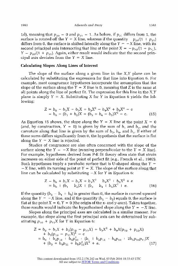
Calculating Slopes Along Lines of Interest
The slope of the surface along a given line in the X,Y plane can be
calculated by substituting the expression for that line into Equation 6. For
example, most congruence hypotheses incorporate the assumption that the
slope of the surface along the Y = X line is 0, meaning that Z is the same at
all points along the line of perfect fit. The expression for this line in the X,Y
plane is simply Y = X. Substituting X for Y in Equation 6 yields the fol-
lowing:
Z = bo + b1X + b2X b3X2 + b4X2 + b5X2 + e
= bo + (b3 + b2)X (b3 + b + b5)X2 + e. (15)
As Equation 15 shows, the slope along the Y = X line at the point X = 0
(and, by construction, Y = 0) is given by the sum of b1 and b2, and the
curvature along that line is given by the sum of b3, b4, and b5. If either of
these sums differs significantly from 0, the hypothesis that the surface is flat
along the Y = X line is rejected. Studies of congruence are also often concerned with the slope of the
surface along the Y = -X line (running perpendicular to the Y = X line). For example, hypotheses derived from P-E fit theory often state that strain
increases on either side of the point of perfect fit (e.g., French et al., 1982). Such hypotheses imply a parabolic surface that is U-shaped along the Y =
-X line, with its turning point at Y = X. The slope of the surface along that
line can be calculated by substituting -X for Y in Equation 6:
Z = bo + b1X - b2X + b3X2 - b4X2 + b5X2 + e = bo + (b - b2)X + (b3
- b4 + b5)X2 + e. (16)
If the quantity (b3 - b4 + b5) is greater than 0, the surface is curved upward
along the Y = -X line, and if the quantity (b1 - b2) equals 0, the surface is
flat at the point X = 0, Y = 0 (the origin of the x- and y-axes). Taken together, these results would indicate the hypothesized slope along the Y = -X line.
Slopes along the principal axes are calculated in a similar manner. For
example, the slope along the first principal axis can be determined by sub-
stituting P1o + p1lX for Y in Equation 6:
Z = bo + b1X + b2(pio + p1X) + b3X2 + b4X(plo + pl1X) + b5(pio + p11X)2 + e
= b bo + b2 b5p2o + (bl + b2p11 + b4pla + 2b5PloPll)X + (b3 + b4p11 + b5p21)X2 + e. (17)
1993 1593
This content downloaded from 152.2.176.242 on Wed, 03 Feb 2016 18:33:43 UTCAll use subject to JSTOR Terms and Conditions
Academy of Management Journal
As Equation 17 shows, the slope at the point where X = 0 (that is, where the
first principal axis crosses the y-axis) is given by the quantity (b1 + b2p11 +
b4P10 + 2b5p10Pl), and the curvature is given by (b3 + b4p11 + b5p21). The
slope along the second principal axis can be calculated by replacing p1o and
P11 with P20 and P21, respectively, in Equation 17, which yields the follow-
ing:
Z = bo + b1X + b2(p20 + P21X) + b3X2 + b4X(P20 + P21X) + b5(P20 + P21X)2 + e
= bo + b22 + bp2 + (bl + b2P21 + b4P20 + 2b5P20P21)X + (b3 + b4p21 + b5p21)X2 + e. (18)
Tests of Significance
Tests of significance for expressions involving linear combinations of
regression coefficients, such as those preceding X and X2 in Equations 15
and 16, can be readily conducted because the standard errors for these ex-
pressions can be derived using ordinary rules for calculating the variance of
a linear combination of random variables (e.g., DeGroot, 1975; Neter,
Wasserman, & Kutner, 1989). However, expressions involving products and
ratios of regression coefficients, such as formulas for the stationary point,
principal axes, and slopes along the principal axes, cannot be tested using conventional procedures because formulas for the standard errors of these
expressions are not generally available (Peddada, 1992). When the formula for the standard error of an expression is unavailable,
nonparametric procedures, such as the jackknife and bootstrap, are applica- ble (Efron, 1982; Efron & Gong, 1983; Tukey, 1958). For this article, we used
the jackknife for its computational ease and demonstrated ability to approx- imate known standard errors (Efron & Gong, 1983; Peddada, 1992). The
procedure used to compute standard errors using the jackknife is described
in the Appendix.
AN EMPIRICAL EXAMPLE
To illustrate the framework described here, we used data from the clas-
sic person-environment fit study conducted by French and colleagues (1982) and reanalyzed by Edwards and Harrison (1993). Regression coefficients
from the six equations reported in Table 1 were used to calculate the sta-
tionary points, principal axes, and slopes along four lines, including Y = X, Y = -X, and the first and second principal axes. We tested the slopes along the Y = X and Y = -X lines using standard procedures for linear combi-
nations of regression coefficients (Neter et al., 1989) and tested the slopes
along the principal axes and the locations of the stationary points and prin-
cipal axes using the jackknife procedure. Tables 2 and 3 present results of
these analyses, and Figures 3a-3f show plots of all six surfaces (for job
complexity, we reversed the scaling of the x- and y-axes to permit a better
view of the surfaces). To interpret the results for each surface, we proceeded as follows. First,
1594 December
This content downloaded from 152.2.176.242 on Wed, 03 Feb 2016 18:33:43 UTCAll use subject to JSTOR Terms and Conditions
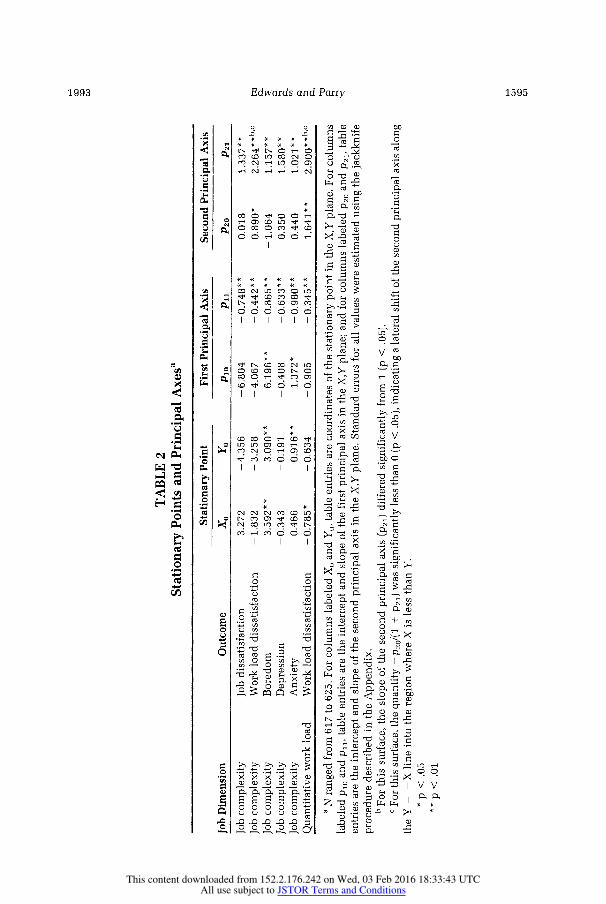
TABLE 2
Stationary Points and Principal Axesa
Stationary Point First Principal Axis Second Principal Axis
Job Dimension Outcome Xo YO Pio Pio P20 P21
Job complexity Job dissatisfaction -3.272 -4.356 - 6.804 - 0.748* * 0.018 1.337 *
Job complexity Work load dissatisfaction -1.832 -3.258 -4.067 -0.442** 0.890* 2.264**b,c
Job complexity Boredom 3.592** 3.090** 6.196** -0.865** -1.064 1.157**
Job complexity Depression -0.343 -0.191 - 0.408 - 0.633** 0.350 1.580**
Job complexity Anxiety 0.466 0.916** 1.372* -0.980** 0.440 1.021**
Quantitative work load Work load dissatisfaction -0.785* -0.634 -0.905 -0.345** 1.641** 2.900**b'c
a N ranged from 617 to 625. For columns labeled Xo and Yo, table entries are coordinates of the stationary point in the X,Y plane. For columns
labeled plo and P11, table entries are the intercept and slope of the first principal axis in the X,Y plane; and for columns labeled P20 and P21, table
entries are the intercept and slope of the second principal axis in the X,Y plane. Standard errors for all values were estimated using the jackknife
procedure described in the Appendix. b For this surface, the slope of the second principal axis (P21) differed significantly from 1 (p < .05). c For this surface, the quantity
- p2/(1 + P21) was significantly less than 0 (p < .05), indicating a lateral shift of the second principal axis along
the Y = - X line into the region where X is less than Y.
p < .05 *
p < .01
nM. Q
CL
11
rn
n. 0
cn
Ul
This content downloaded from 152.2.176.242 on Wed, 03 Feb 2016 18:33:43 UTCAll use subject to JSTOR Terms and Conditions
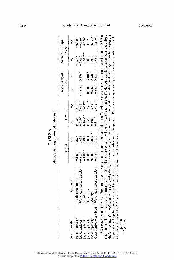
TABLE 3
Slopes Along Lines of Interesta
First Principal Second Principal Y = X Y = -X Axis Axis
Job Dimension Outcome ax ax2 ax ax 2 ax ax2 ax ax2
Job complexity Job dissatisfaction -0.198** -0.017 0.035 0.416** -0.238** -0.036
Job complexity Work load dissatisfaction -0.123* 0.029 0.329** 0.442** -1.118 0.258** -0.498 -0.136
Job complexity Boredom -0.490** 0.071* -0.444** 0.484** -0.578** 0.080*
Job complexity Depession -0.006 -0.024 0.051 0.173** 0.088 0.128* -0.042 -0.061
Job complexity Anxiety 0.088* -0.062** 0.105 0.244** -0.223 0.239* 0.059 -0.064**
Quantitative work load Work load dissatisfaction -0.078 -0.109 0.831** 0.693** 0.827* 0.527** -2.652 -1.690
a N ranged from 617 to 625. For each line, a, repesents the computed coefficient on X, and a,2 represents the computed coefficient on X2. For
example, for the Y = X line, ax represents (b, + b2) and ax2 represents (b3 + b+4 b5) (see Equation 17). We derived standard errors for slopes along the Y = X and Y = -X lines using standard rules for the variance of a linear combination of random variables and calculated standard errors for
slopes along the principal axes using the jackknife procedure described in the Appendix. The slope along a principal axis is not reported when the
axis does not cross the X,Y plane in the range of the component measures.
p < .05
** p < .01
C-^
CD a?
0 a
Dc
CD
B cc
a
:z
Q ol
CD 0 CD
CD
This content downloaded from 152.2.176.242 on Wed, 03 Feb 2016 18:33:43 UTCAll use subject to JSTOR Terms and Conditions
Edwards and Parry
we examined the coordinates of the stationary point to determine whether
the surface was centered at the origin of the x- and y-axes (that is, the point X = 0, Y = 0). Next, we examined the intercepts and slopes of the principal axes of the surface. Tests of whether the slopes of the principal axes differed
from 0 were supplemented by tests of whether the slope of the second prin-
cipal axis (p21) differed from 1 and whether the second principal axis was
shifted laterally along the Y = - X line, as indicated by the quantity - p2/(1 + P21). We conducted these additional tests because P-E fit theory states that
strain is minimized when actual and desired amounts of job attributes are
equal (French et al., 1982), implying a U-shaped surface with its second
principal axis (the region of minimum strain) running along the Y = X line
(Figure ld). Third, we examined the slope of the surface along the Y - X and
Y = -X lines. Slopes along the principal axes were also considered when
the principal axes differed from the Y = X and Y = -X lines but still passed
through the X,Y plane within the range of the X and Y measures. Although this procedure emphasized only a subset of the results reported in Tables 2
and 3, the remaining results can be examined to obtain a more complete
understanding of each surface.
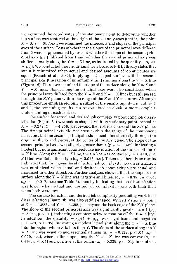
The surface for actual and desired job complexity predicting job dissat-
isfaction (Figure 3a) was saddle-shaped, with its stationary point located at
X = - 3.272, Y = -4.356, just beyond the far-back corner of the X,Y plane. The first principal axis did not cross within the range of the component measures, but the second principal axis passed almost exactly through the
origin of the x- and y-axes, at the center of the X,Y plane. The slope of the
second principal axis was slightly greater than 1 (p 21 = 1.337), indicating a
modest but nonsignificant counterclockwise rotation of the surface off the Y
= X line. Along the Y = -X line, the surface was convex (a2 = 0.416, p <
.01) but was flat at the origin (ax = 0.035, n.s.). Taken together, these results
indicated that, for a given level of actual job complexity, job dissatisfaction
was minimized when actual and desired job complexity were equal and
increased in either direction. Further analyses showed that the slope of the
surface along the Y = X line was negative and linear (a = - 0.198, p < .01;
ax2 = -0.017, n.s.; see Table 3), thereby indicating that job dissatisfaction
was lower when actual and desired job complexity were both high than
when both were low.
The surface for actual and desired job complexity predicting work load
dissatisfaction (Figure 3b) was also saddle-shaped, with its stationary point at X = - 1.832 and Y - - 3.258, just beyond the back edge of the X,Y plane. The slope of the second principal axis was significantly greater than 1 (p21 = 2.264, p < .01), indicating a counterclockwise rotation off the Y = X line.
In addition, the quantity -p20/(1 + P21) was significant and negative
(-0.273, p < .05), indicating a modest lateral shift along the Y = -X line
into the region where X is less than Y. The slope of the surface along the Y = X line was negative and essentially linear (ax = -0.123, p < .05; a2 =
0.029, n.s.), whereas the slope along the Y = -X line was convex (ax2 =
0.442, p < .01) and positive at the origin (ax = 0.329, p < .01). In contrast,
1993 1597
This content downloaded from 152.2.176.242 on Wed, 03 Feb 2016 18:33:43 UTCAll use subject to JSTOR Terms and Conditions
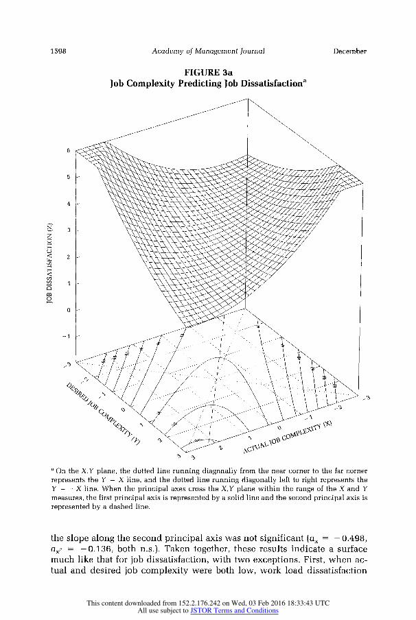
Academy of Management Journal
FIGURE 3a
Job Complexity Predicting Job Dissatisfactiona
L)
3-
a On the X,Y plane, the dotted line running diagonally from the near corner to the far corner
represents the Y = X line, and the dotted line running diagonally left to right represents the
Y = -X line. When the principal axes cross the X,Y plane within the range of the X and Y
measures, the first principal axis is represented by a solid line and the second principal axis is
represented by a dashed line.
the slope along the second principal axis was not significant (ax = -0.498,
ax2 = -0.136, both n.s.). Taken together, these results indicate a surface
much like that for job dissatisfaction, with two exceptions. First, when ac-
tual and desired job complexity were both low, work load dissatisfaction
tuladdsrdjbcop e i ywrbthl,wor loa d isstifcto
1598 December
This content downloaded from 152.2.176.242 on Wed, 03 Feb 2016 18:33:43 UTCAll use subject to JSTOR Terms and Conditions
Edwards and Parry
FIGURE 3b
Job Complexity Predicting Work Load Dissatisfactiona
4
N
Z
U
CL
Cl)
-3
cn
c4
c/4
CD
3
2
1
0
-1
2
a On the X,Y plane, the dotted line running diagonally from the near corner to the far corner
represents the Y = X line, and the dotted line running diagonally left to right represents the
Y = -X line. When the principal axes cross the X,Y plane within the range of the X and Y
measures, the first principal axis is represented by a solid line and the second principal axis is
represented by a dashed line.
was lowest when actual job complexity exceeded desired job complexity; but when actual and desired job complexity were both high, work load
dissatisfaction was lowest when actual job complexity fell short of desired
job complexity. Second, work load dissatisfaction was somewhat greater
,3
1993 1599
This content downloaded from 152.2.176.242 on Wed, 03 Feb 2016 18:33:43 UTCAll use subject to JSTOR Terms and Conditions
Academy of Management Journal
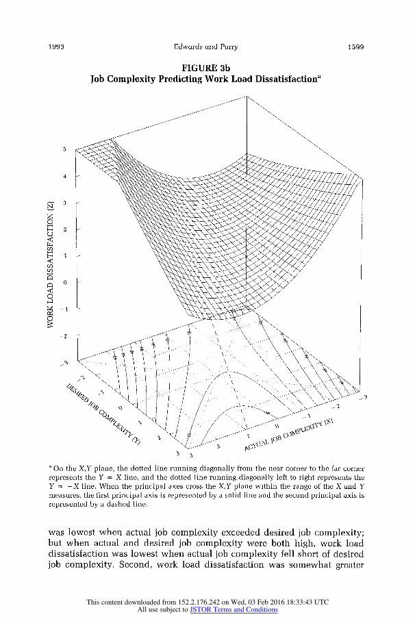
FIGURE 3c
Job Complexity Predicting Boredoma
3
2
1
N-
O
CQ 0
-1
-2
-3
a On the X,Y plane, the dotted line running diagonally from the near corner to the far corner
represents the Y = X line, and the dotted line running diagonally left to right represents the
Y = -X line. When the principal axes cross the X,Y plane within the range of the X and Y
measures, the first principal axis is represented by a solid line and the second principal axis is
represented by a dashed line.
when actual job complexity exceeded desired job complexity than when it
fell short of desired job complexity. The surface for actual and desired job complexity predicting boredom
(Figure 3c) was convex, with its stationary point at X = 3.592, Y = 3.090,
December 1600
This content downloaded from 152.2.176.242 on Wed, 03 Feb 2016 18:33:43 UTCAll use subject to JSTOR Terms and Conditions
Edwards and Parry
FIGURE 3d
Job Complexity Predicting Depressiona
z
/ 13
0
a On the X,Y plane, the dotted line running diagonally from the near corner to the far corner
represents the Y = X line, and the dotted line running diagonally left to right represents the
Y = -X line. When the principal axes cross the X,Y plane within the range of the X and Y
measures, the first principal axis is represented by a solid line and the second principal axis is
represented by a dashed line.
just outside the near corner of the X,Y plane. The slope of the second prin- cipal axis was 1.157, representing a slight but nonsignificant rotation from
the Y = X line. The slope along the Y = X line was slightly convex (aX2 =
0.071, p < .05) and negative at the origin (ax = - 0.490, p < .01), whereas the 0.071, p < .05) and negative at the origin (ax =z -0.490, p < .01), whereas the
1993 1601
This content downloaded from 152.2.176.242 on Wed, 03 Feb 2016 18:33:43 UTCAll use subject to JSTOR Terms and Conditions
Academy of Management Journal
FIGURE 3e
Job Complexity Predicting Anxietya
N
H
u
-3
3
a On the X,Y plane, the dotted line running diagonally from the near corner to the far corner
represents the Y = X line, and the dotted line running diagonally left to right represents the
Y = -X line. When the principal axes cross the X,Y plane within the range of the X and Y
measures, the first principal axis is represented by a solid line and the second principal axis is
represented by a dashed line.
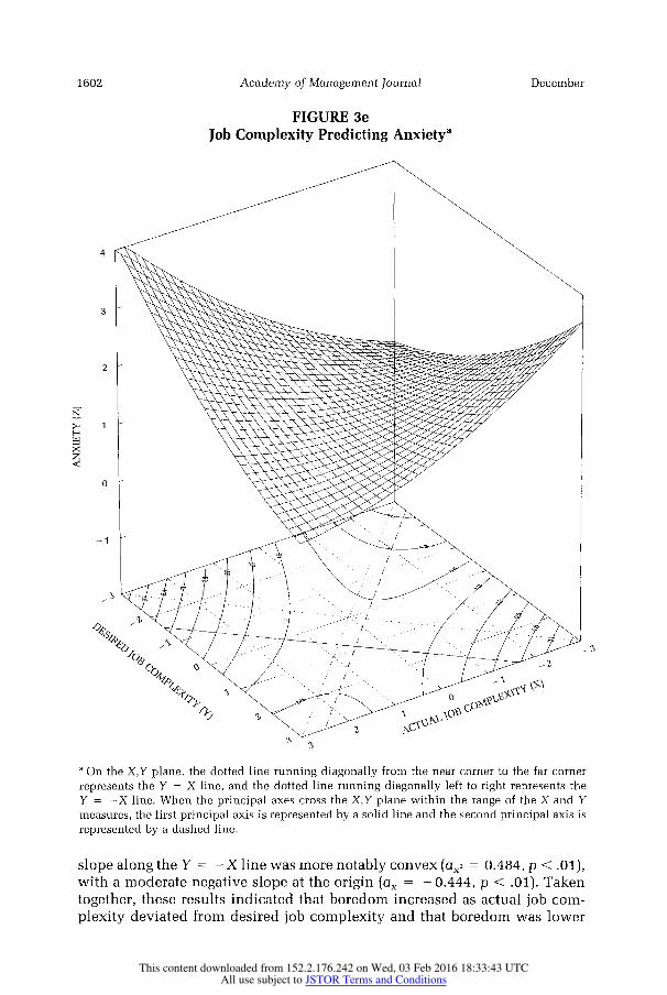
slope along the Y = -X line was more notably convex (aX2 = 0.484, p < .01), with a moderate negative slope at the origin (ax = - 0.444, p < .01). Taken
together, these results indicated that boredom increased as actual job com-
plexity deviated from desired job complexity and that boredom was lower
1602 December
This content downloaded from 152.2.176.242 on Wed, 03 Feb 2016 18:33:43 UTCAll use subject to JSTOR Terms and Conditions
Edwards and Parry
FIGURE 3f
Quantitative Work Load Predicting Work Load Dissatisfactiona
a On the X,Y plane, the dotted line running diagonally from the near corner to the far corner
represents the Y = X line, and the dotted line running diagonally left to right represents the
Y = -X line. When the principal axes cross the X,Y plane within the range of the X and Y
measures, the first principal axis is represented by a solid line and the second principal axis is
represented by a dashed line.
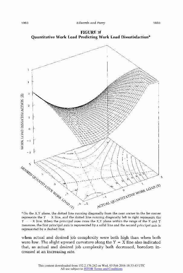
when actual and desired job complexity were both high than when both
were low. The slight upward curvature along the Y = X line also indicated
that, as actual and desired job complexity both decreased, boredom in-
creased at an increasing rate.
1993 1603
This content downloaded from 152.2.176.242 on Wed, 03 Feb 2016 18:33:43 UTCAll use subject to JSTOR Terms and Conditions
Academy of Management Journal
The surface for actual and desired job complexity predicting depression
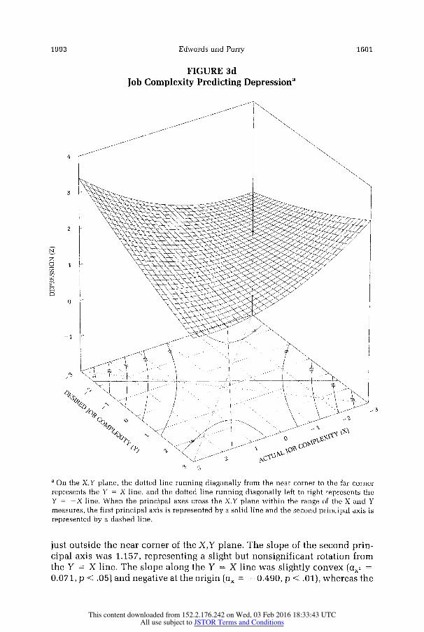
(Figure 3d) was saddle-shaped, with its stationary point at X = - 0.343, Y =
- 0.191, near the origin of the x- and y-axes. The slope of the first and second
principal axes did not differ from - 1 and 1, respectively (p11 = - 0.633, p21 = 1.580), indicating no appreciable rotation off the Y = -X and Y = X
lines. The surface was flat along the Y = X line (ax = - 0.006, ax2 = -0.024, both n.s.) and convex along the Y = -X line (ax = 0.051, n.s., aX2 = 0.173,
p < .01). Overall, these results essentially indicated that depression in-
creased as actual job complexity deviated from desired job complexity. This
finding is corroborated by the difference in the R2 between the constrained
and unconstrained equations reported in Table 1, which, although statisti-
cally significant, was relatively small (.017). The surface for actual and desired job complexity predicting anxiety
(Figure 3e) was also saddle-shaped, with its stationary point at X = 0.466, Y
= 0.916, shifted somewhat from the origin along the y-axis. The slopes of the
first and second principal axes (p1l and P21) were - 0.980 and 1.021, respec-
tively, corresponding very closely to -1 and 1. However, the intercept of
the first principal axis differed from 0 (plo = 1.372, p < .05), a finding
that, combined with the location of YO, indicated a lateral shift along the
y-axis. The surface was convex along the first principal axis (ax2 = 0.239,
p < .01) but essentially flat where it crossed the y-axis (ax = -0.223, n.s.). In contrast, the surface was slightly concave along the Y = X line (a2
=
- 0.062, p < .01), with a modest positive slope where it crossed the y-axis
(ax = 0.088, p < .05). These results indicated that anxiety increased as
actual job complexity deviated from desired job complexity and also that
anxiety was higher when actual and desired job complexity were both mod-
erate (in this case, about .7 units) than when they were both either high or low.
Finally, the surface for actual and desired quantitative work load pre-
dicting work load dissatisfaction (Figure 3f) was saddle-shaped, with its
stationary point at X = -0.785, Y = -0.634, shifted slightly downward
along the Y = X line. The slopes of the first and second principal axes (Pll and P21) were -0.345 and 2.900, respectively, indicating a marked counter-
clockwise rotation. In addition, the quantity -p20/(1 + P21) was significant and negative (-0.421, p < .05) indicating a lateral shift along the Y = -X
line into the region where X is less than Y. The surface was convex along the
first principal axis (ax2 = 0.527, p < .01) and positively sloped where it
crossed the y-axis (ax = 0.827, p < .05). In contrast, the surface was concave
along the second principal axis and negatively sloped where it crossed the
y-axis, but neither ax nor ax2 was significant, due to the sizable jackknife estimates of their standard errors. Essentially, these results indicated that, when actual and desired work load were below their scale midpoints, work
load dissatisfaction increased as actual work load deviated from desired
work load, but when actual and desired work load were above their scale
midpoints, work load dissatisfaction was lowest when actual work load was
somewhat less than desired work load. In addition, work load dissatisfaction
1604 December
This content downloaded from 152.2.176.242 on Wed, 03 Feb 2016 18:33:43 UTCAll use subject to JSTOR Terms and Conditions
Edwards and Parry
was higher when actual work load exceeded desired work load than when it
fell short of desired work load.
DISCUSSION
This article presents a general framework for testing and interpreting
quadratic regression equations within the study of congruence in organiza- tional research. These equations avoid many problems with difference
scores but permit direct tests of conceptual models difference scores are
intended to represent (Edwards, in press). Unfortunately, these equations often yield patterns of coefficients that are difficult to interpret, particularly when models specified a priori are not supported. The framework presented here shows how coefficients from quadratic regression equations can be
used to comprehensively describe and test the surfaces they imply. Thus, this framework clarifies the interpretation of quadratic regression equations and permits rigorous evaluation of conceptual models relevant to the study of congruence, including models that are substantially more complex than
those represented by difference scores.
The incremental contribution of the framework presented here may be
seen by comparing our results to those reported by French and colleagues
(1982; see also Caplan et al., 1980), who analyzed the relationship between
P-E fit and strain using various transformations of algebraic and squared difference scores. French and colleagues concluded that the functional form
relating actual and desired job complexity to the five indexes of strain re-
ported in Table 1 was essentially U-shaped. They elaborated this general conclusion by stating that too little job complexity exhibited a stronger re-
lationship with boredom, whereas too much job complexity exhibited stron-
ger relationships with work load dissatisfaction, depression, and anxiety. French and colleagues also reported that the functional form rebuting actual
and desired quantitative work load to work load dissatisfaction was
U-shaped, with stronger effects for excess work load.
Subsequent reanalyses by Edwards and Harrison (1993) using the poly- nomial regression procedure (Edwards, in press) indicated that, with few
exceptions, the constraints imposed by the difference scores used by French
and colleagues were rejected. Plots of the surfaces corresponding to the
equations reported in Table 1 suggested various deviations from the surface
indicated by the squared difference (Figure Id), such as slopes along the Y = X line, lateral shifts, and counterclockwise rotations. However, Edwards
and Harrison were forced to base their conclusions primarily on visual in-
spection of these surfaces because the framework presented here was un-
available.
By applying this framework, we can now draw firm conclusions regard-
ing the surfaces corresponding to the equations reported in Table 1. For
example, consistent with the findings reported by French and colleagues
(1982), all six surfaces were U-shaped, evidenced by the significant, positive coefficients on ax2 along the Y = -X line (or, for rotated surfaces, along the
first principal axis). Furthermore, excess job complexity and quantitative
1993 1605
This content downloaded from 152.2.176.242 on Wed, 03 Feb 2016 18:33:43 UTCAll use subject to JSTOR Terms and Conditions
Academy of Management Journal
work load exacerbated work load dissatisfaction, as shown by the lateral
shifts in these surfaces along the Y = -X line, into the region where X is less
than Y. However, contrary to French and colleagues' findings, the functions
relating actual and desired job complexity to boredom, depression, and anx-
iety were essentially symmetric. This is shown by the locations of the second
principal axes of these surfaces, which did not deviate from the Y = X line
(P21 and the quantity - p20/(1 + P21) did not differ significantly from 1 and
0, respectively). In addition, the surfaces relating job complexity and quan- titative work load to work load dissatisfaction were rotated counterclock-
wise, indicating that, when actual and desired amounts of these job dimen-
sions were low, a slight excess minimized work load dissatisfaction, whereas when actual and desired amounts were high, a slight deficiency minimized work load dissatisfaction. Furthermore, several surfaces were
sloped along the line of perfect fit (the Y = X line), including a positive slope for actual and desired job complexity predicting anxiety and negative slopes for actual and desired job complexity predicting job dissatisfaction, work
load dissatisfaction, and boredom. These additional findings, although not
reported by French and colleagues, are nonetheless consistent with P-E fit
theory, which suggest that strain may vary along the Y = X line and be
minimized at points other than perfect fit (Caplan, 1983; French et al., 1982;
Harrison, 1978, 1985). By applying the framework presented here in other
studies of congruence, researchers are likely to find theoretically relevant
effects that have previously gone undetected.
The framework presented here was illustrated using paired measures of
individual-level constructs. This framework can, however, be readily ap-
plied to other forms of congruence research. For example, numerous studies
have examined congruence between organization-level constructs, such as
technology and structure (Alexander & Randolph, 1985; Dewar & Werbel,
1979; Fry & Slocum, 1984), an organization and its environment (Anderson & Zeithaml, 1984; Miller, 1991), and actual and ideal scores on measures of
organizational strategy (Venkatraman, 1990; Venkatraman & Prescott, 1990) or structure (Drazin & Van de Ven, 1985; Gresov, 1989). Naturally, the effects
of congruence between these constructs can be readily examined using the
framework described here, because this framework is applicable to measures
of any paired constructs of interest in congruence research.
Furthermore, many studies have examined the effects of congruence
along multiple dimensions, usually expressed in terms of a profile similarity index (e.g., Drazin & Van de Ven, 1985; Gresov, 1989; Rounds et al., 1987;
Sparrow, 1989; Turban & Jones, 1988; Venkatraman, 1990; Venkatraman &
Prescott, 1990; Zalesny & Kirsch, 1989). Unfortunately, using profile simi-
larity indexes to represent congruence introduces numerous methodological
problems (Cronbach, 1958; Edwards, in press; Johns, 1981; Lykken, 1956;
Nunnally, 1962). Many of these problems can be avoided by examining
congruence not between entire profiles, but between specific, paired dimen-
sions, using quadratic regression equations to depict the hypothesized rela-
tionship (Cronbach, 1958; Edwards, 1993). If separate equations are used for
each pair of dimensions, the framework presented here can be directly ap-
1606 December
This content downloaded from 152.2.176.242 on Wed, 03 Feb 2016 18:33:43 UTCAll use subject to JSTOR Terms and Conditions
Edwards and Parry
plied. If multiple pairs are included in the same equation, the framework can
be applied to coefficients from terms corresponding to each pair. In this case,
the surface represented by each pair of dimensions represents the joint ef-
fects of those dimensions on the dependent variable, holding the effects of
all other dimensions constant.
Although the framework presented here should prove useful in future
studies of congruence, it nonetheless has several shortcomings. First, some
aspects of the framework, particularly the jackknife procedure, are compu-
tationally intensive. In most cases, this should not pose major difficulties,
given the widespread availability of high-speed computers. Second, the
framework relies on numerous tests of significance, which may inflate Type I error rates. This may be controlled using the Bonferroni correction (Harris,
1985) or more powerful alternatives, such as the sequential procedures de-
scribed by Holm (1979) and Holland and Copenhaver (1988).
Third, the jackknife procedure tends to overestimate known standard
errors (Efron & Gong, 1983). This problem is accentuated by the presence of
outliers, which may dramatically influence coefficient estimates and hence
increase the variability of the coefficient estimates yielded by the jackknife
procedure. This problem can be minimized by screening data for influential
cases prior to analysis and either eliminating them or, if a large number is
detected, modeling them separately using an indicator variable (Belsley,
Kuh, & Welsch, 1980).
Fourth, like any application of regression analysis, this framework is
based on the assumption that the component variables are measured without
error (Pedhazur, 1982). This assumption can be relaxed when structural
equations modeling is used (Bollen, 1989; Joreskog & Sorbom, 1988). The
resulting structural coefficients can be interpreted using the framework pre- sented here, with the caveat that the x-, y-, and z-axes represent latent con-
structs rather than manifest variables. However, procedures for estimating structural coefficients on curvilinear and interactive terms are rather com-
plex and have yet to attain widespread use (Bollen, 1989; Hayduk, 1987;
Kenny & Judd, 1984). Furthermore, the jackknife procedure would require
recalculating the sample covariance matrix N times, adding significant com-
putational requirements when large samples are used. At this stage, perhaps the most advisable procedure is to ensure that component measures are
highly reliable prior to analysis, thereby minimizing problems resulting from measurement error at subsequent stages (Edwards, in press).
A final issue is the interpretation of regression coefficients on lower-
order terms, such as b1 and b2 in Equation 6, in the presence of higher-order terms. These coefficients are scale-dependent, meaning that adding or sub-
tracting a constant to X or Y will change the estimated values and signifi- cance levels of b1 and b2 (Arnold & Evans, 1979; Cohen, 1978). Although this
dependence may seem to render the interpretation of b1 and b2 meaningless, it simply reflects the fact that these coefficients represent conditional rela-
tionships, indicating the slope of the surface where both X and Y equal 0
(Aiken & West, 1991; Jaccard et al., 1990). Rescaling X and Y simply shifts
the origin of the x- and y-axes, so that b1 and b2 describe the slope at a
1993 1607
This content downloaded from 152.2.176.242 on Wed, 03 Feb 2016 18:33:43 UTCAll use subject to JSTOR Terms and Conditions
Academy of Management Journal
different point on the surface. If rescaling moves the origin beyond the range of X and Y, then b1 and b2 are obviously not meaningful, because they
represent estimates extrapolated beyond the bounds of the data. However,
rescaling within the range of X and Y produces values of b1 and b2 that may
yield useful interpretations. For example, if X and Y are centered at their
means, b1 and b2 represent the slope of the surface at the mean of both X and
Y (Cronbach, 1987). X and Y can be centered at other useful values, such as
one standard deviation above or below their means (cf. Cohen & Cohen, 1983: 325). In our analyses, we centered X and Y at their scale midpoints, because these values are not sample-dependent and yield useful interpreta- tions of bI and b2 (the slope of the surface at the center of the plane bounded
by the X and Y measures). It should be emphasized that these rescalings do
not affect the correspondence between the surface and the data, because the
calculated locations of the stationary point and principal axes change ac-
cordingly with the rescaling of X and Y. For more detailed discussions of the
interpretation of coefficients on lower-order terms in polynomial regression
equations, see Aiken and West (1991) and Jaccard and colleagues (1990).
CONCLUSION
The study of congruence in organizational research is currently at a
critical juncture. For decades, research in this area has relied on difference
scores, which introduce numerous substantive and methodological prob- lems. These problems are sufficiently serious to render much of this research
inconclusive. For example, a recent review of person-job fit studies con-
ducted from 1960 through 1989 (Edwards, 1991) revealed that, due to the
widespread use of difference scores, the results of these studies are largely inconclusive. This situation is not unique to the person-job fit literature but
is evident in virtually every area of organizational research that uses differ-
ence scores to examine congruence (Edwards, in press; Mowday, 1987; Wanous et al., 1992; Van de Ven & Drazin, 1985). Fortunately, procedures such as the polynomial regression approach and the framework presented here are now available that avoid many problems with difference scores and
more fully address questions of conceptual relevance in congruence re-
search. If these procedures gain widespread acceptance, problems attribut-
able to the use of difference scores in congruence research may be overcome, and significant theoretical and empirical advances are likely to occur.
REFERENCES
Aiken, L. A., & West, S. G. 1991. Multiple regression: Testing and interpreting interactions.
Newbury Park, CA: Sage.
Alexander, J. W., & Randolph, W. A. 1985. The fit between technology and structure as a pre- dictor of performance in nursing subunits. Academy of Management Journal, 28: 844-859.
Anderson, C., & Zeithaml, C. P. 1984. Stage of product life cycle, business strategy, and business
performance. Academy of Management Journal, 27: 5-24.
Arnold, H. J., & Evans, M. G. 1979. Testing multiplicative models does not require ratio scales.
Organizational Behavior and Human Performance, 24: 41-59.
1608 December
This content downloaded from 152.2.176.242 on Wed, 03 Feb 2016 18:33:43 UTCAll use subject to JSTOR Terms and Conditions
1993 Edwards and Parry 1609
Belsley, D. A., Kuh, E., & Welsch, R. E. 1980. Regression diagnostics: Identifying influential data and sources of collinearity. New York: Wiley.
Bollen, K. A. 1989. Structural equations with latent variables. New York: Wiley.
Box, G. E. P., & Draper, N. R. 1987. Empirical model-building and response surfaces. New
York: Wiley.
Caplan, R. D. 1983. Person-environment fit: Past, present, and future. In C. L. Cooper (Ed.), Stress research: 35-78. New York: Wiley.
Caplan, R. D., Cobb, S., French, J. R. P., Jr., Harrison, R. V., & Pinneau, S. R. 1980. Job demands
and worker health: Main effects and occupational differences. Ann Arbor, MI: Institute
for Social Research.
Chatman, J. A. 1991. Matching people and organizations: Selection and socialization in public
accounting firms. Administrative Science Quarterly, 36: 459-484.
Chiang, A. C. 1974. Fundamental methods of mathematical economics (2d ed.). New York:
McGraw-Hill.
Cherrington, D. J., & England, J. L. 1980. The desire for an enriched job as a moderator of the
enrichment-satisfaction relationship. Organizational Behavior and Human Performance, 25: 139-159.
Cohen, J. 1978. Partialed products are interactions: Partialed powers are curve components.
Psychological Bulletin, 85: 858-866.
Cohen, J., & Cohen, P. 1983. Applied multiple regression/correlation analysis for the behav-
ioral sciences (2d ed.). Hillsdale, NJ: Erlbaum.
Cronbach, L. J. 1958. Proposals leading to analytic treatment of social perception scores. In R.
Tagiuri & L. Petrullo (Eds.), Person perception and interpersonal behavior: 353-379.
Stanford, CA: Stanford University Press.
Cronbach, L. J. 1987. Statistical tests for moderator variables: Flaws in analyses recently pro-
posed. Psychological Bulletin, 102: 414-417.
Cronbach, L. J., & Furby, L. 1970. How we should measure "change"-or should we? Psycho-
logical Bulletin, 74: 68-80.
DeGroot, M. H. 1975. Probability and statistics. Reading, MA: Addison-Wesley.
Dewar, R., & Werbel, J. 1979. Universalistic and contingency predictions of employee satisfac-
tion and conflict. Administrative Science Quarterly, 24: 426-448.
Dittrich, J. E., & Carrell, M. R. 1979. Organizational equity perceptions, employee job satisfac-
tion, and departmental absence and turnover rates. Organizational Behavior and Human
Performance, 24: 29-40.
Dougherty, T. W., & Pritchard, R. D. 1985. The measurement of role variables: Exploratory examination of a new approach. Organizational Behavior and Human Decision Process, 35: 141-155.
Drazin, R., & Van de Ven, A. H. 1985. Alternative forms of fit in contingency theory. Admin-
istrative Science Quarterly, 30: 514-539.
Edwards, J. R. 1991. Person-job fit: A conceptual integration, literature review, and method-
ological critique. In C. L. Cooper & I. T. Robertson (Eds.), International review of indus-
trial and organizational psychology, vol. 6: 283-357. New York: Wiley.
Edwards, J. R. 1992. An examination of major variations within the person-environment fit
approach to stress. Working paper, Darden Graduate School of Business, University of
Virginia, Charlottesville.
Edwards, J. R. 1993. Problems with the use of profile similarity indices in the study of congru- ence in organizational research. Personnel Psychology, 46: 641-665.
This content downloaded from 152.2.176.242 on Wed, 03 Feb 2016 18:33:43 UTCAll use subject to JSTOR Terms and Conditions
1610 Academy of Management Journal December
Edwards, J. R. in press. The study of congruence in organizational behavior research: Critique and a proposed alternative. Organizational Behavior and Human Decision Process.
Edwards, J. R., & Cooper, C. L. 1990. The person-environment fit approach to stress: Recurring
problems and some suggested solutions. Journal of Organizational Behavior, 10: 293-
307.
Edwards, J. R., & Harrison, R. V. 1993. Job demands and worker health: A three-dimensional
reexamination of the relationship between person-environment fit and strain. Journal of
Applied Psychology, 78: 628-648.
Efron, B. 1982. The jackknife, the bootstrap, and other resampling plans. Philadelphia: So-
ciety for Industrial and Applied Math.
Efron, B., & Gong, G. 1983. A leisurely look at the bootstrap, the jackknife, and cross-validation.
American Statistician, 37: 36-48.
French, J. R. P., Jr., Caplan, R. D., & Harrison, R. V. 1982. The mechanisms of job stress and
strain. London: Wiley.
Fry, L. W., & Slocum, J. W., Jr. 1984. Technology, structure, and work group effectiveness: A test
of a contingency model. Academy of Management Journal, 27: 221-246.
Gresov, C. 1989. Exploring fit and misfit with multiple contingencies. Administrative Science
Quarterly, 34: 431-453.
Hackman, J. R., & Oldham, G. R. 1980. Work redesign. Reading, MA: Addison-Wesley.
Harris, R. J. 1985. A primer of multivariate statistics (2d ed.) New York: Academic Press.
Harrison, R. V. 1978. Person-environment fit and job stress. In C. L. Cooper & R. Payne (Eds.), Stress at work: 175-205. New York: Wiley.
Harrison, R. V. 1985. The person-environment fit model and the study of job stress. In T. A.
Beehr & R. S. Bhagat (Eds.), Human stress and cognition in organizations: 23-55. New
York: Wiley.
Hayduk, L. A. 1987. Structural equation modeling with LISREL. Baltimore: Johns Hopkins
University Press.
Holland, B. S., & Copenhaver, M. D. 1988. Improved Bonferroni-type multiple testing proce- dures. Psychological Bulletin, 104: 145-149.
Holm, S. 1979. A simple sequentially rejective multiple test procedure. Scandinavian Journal
of Statistics, 6: 65-70.
Jaccard, J., Turrisi, R., & Wan, C. K. 1990. Interaction effects in multiple regression. Newbury
Park, CA: Sage.
Johns, G. 1981. Difference score measures of organizational behavior variables: A critique.
Organizational Behavior and Human Performance, 27: 443-463.
Joreskog, K. G., & Sorbom, D. 1988. LISREL 7. Chicago: SPSS.
Karasek, R. A. 1979. Job demands, job decision latitude and mental strain: Implications for job
redesign. Administrative Science Quarterly, 24: 285-308.
Karasek, R. A., & Theorell, T. 1990. Healthy work: Stress, productivity, and the reconstruction
of working life. New York: Basic Books.
Kenny, D. A., & Judd, C. M. 1984. Estimating the nonlinear and interactive effects of latent
variables. Psychological Bulletin, 96: 201-210.
Kernan, M. C., & Lord, R. G. 1990. Effects of valence, expectancies, and goal-performance dis-
crepancies in single and multiple goal environments. Journal of Applied Psychology, 75:
194-203.
Khuri, A. I., & Cornell, J. A. 1987. Response surfaces: Designs and analyses. New York: Marcel
Dekker.
This content downloaded from 152.2.176.242 on Wed, 03 Feb 2016 18:33:43 UTCAll use subject to JSTOR Terms and Conditions
Edwards and Parry
Kulik, C. T., Oldham, G. R., & Hackman, J. R. 1987. Work design as an approach to person- environment fit. Journal of Vocational Behavior, 31: 278-296.
Liedtka, J. 1989. Value congruence: The interplay of individual and organizational value sys- tems. Journal of Business Ethics, 8: 805-815.
Lykken, D. T. 1956. A method of actuarial pattern analysis. Psychological Bulletin, 53: 102-107.
Meglino, B. M., Ravlin, E. C., & Adkins, C. L. 1989. A work values approach to corporate cul-
ture: A field test of the value congruence process and its relationship to individual out-
comes. Journal of Applied Psychology, 74: 424-434.
Meglino, B. M., Ravlin, E. C., & Adkins, C. L. 1992. The measurement of work value congruence: A field study comparison. Journal of Management, 18: 33-43.
Miller, D. 1991. Stable in the saddle: CEO tenure and the match between organization and
environment. Management Science, 37: 34-52.
Mowday, R. T. 1987. Equity theory predictions of behavior in organizations. In R. Steers & L.
Porter (Eds.), Motivation and work behavior: 89-110. New York: McGraw-Hill.
Neter, J., Wasserman, W., & Kutner, M. H. 1989. Applied linear regression models (2d ed.).
Homewood, IL: Irwin.
Nunnally, J. C. 1962. The analysis of profile data. Psychological Bulletin, 59: 311-319.
Oldham, G. R., Kulik, C. T., Ambrose, M. L., Stepina, L. P., & Brand, J. F. 1986. Relations be-
tween job facet comparisons and employee reactions. Organizational Behavior and Hu-
man Decision Process, 38: 27-47.
Peddada, S. D. 1992. Jackknife variance estimation and bias reduction. Working paper, Di-
vision of Statistics, University of Virginia, Charlottesville.
Pedhazur, E. J. 1982. Multiple regression in behavioral research. New York: Holt.
Reichers, A. E. 1986. Conflict and organizational commitments. Journal of Applied Psychol-
ogy, 71: 508-514.
Rice, R. W., McFarlin, D. B., & Bennett, D. E. 1989. Standards of comparison and job satisfac-
tion. Journal of Applied Psychology, 74: 591-598.
Rounds, J. B., Dawis, R. W., & Lofquist, L. H. 1987. Measurement of person-environment fit and
prediction of satisfaction in the theory of work adjustment. Journal of Vocational Behav-
ior, 31: 297-318.
Scholl, R. W., Cooper, E. A., & McKenna, J. F. 1987. Referent selection in determining equity
perceptions: Differential effects on behavioral and attitudinal outcomes. Personnel Psy-
chology, 40: 113-123.
Sparrow, J. A. 1989. The measurement of job profile similarity for the prediction of transfer of
learning: A research note. Journal of Occupational Psychology, 62: 337-341.
Summers, T. P., & Hendrix, W. H. 1991. Modelling the role of pay equity perceptions: A field
study. Journal of Occupational Psychology, 64: 145-157.
Telly, C. S., French, W. L., & Scott, W. G. 1971. The relationship of inequity to turnover among
hourly workers. Administrative Science Quarterly, 16: 164-172.
Tsui, A. S., & O'Reilly, C. A. 1989. Beyond simple demographic effects: The importance of
relational demography in superior-subordinate dyads. Academy of Management Journal, 32: 402-423.
Tubbs, M. E., & Dahl, J. G. 1991. An empirical comparison of self-report and discrepancy mea-
sures of goal commitment. Journal of Applied Psychology, 76: 708-716.
Tukey, J. W. 1958. Bias and confidence in not quite large samples. Annals of Mathematics and
Statistics, 29: 614.
Turban, D. B., & Jones, A. P. 1988. Supervisor-subordinate similarity: Types, effects, and mech-
anisms. Journal of Applied Psychology, 73: 228-234.
1993 1611
This content downloaded from 152.2.176.242 on Wed, 03 Feb 2016 18:33:43 UTCAll use subject to JSTOR Terms and Conditions
Academy of Management Journal
Vance, R. J., & Colella, A. 1990. Effects of two types of feedback on goal acceptance and personal
goals. Journal of Applied Psychology, 75: 68-76.
Vancouver, J. B., & Schmitt, N. W. 1991. An exploratory examination of person-organization fit:
Organizational goal congruence. Personnel Psychology, 44: 333-352.
Van de Ven, A. H., & Drazin, R. 1985. The concept of fit in contingency theory. In L. L. Cum-
mings & B. M. Staw (Eds.), Research in organizational behavior, vol. 7: 333-365. New
York: JAI Press.
Venkatraman, N. 1990. Performance implications of strategic coalignment: A methodological
perspective. Journal of Management Studies, 27: 19-41.
Venkatraman, N., & Prescott, J. E. 1990. Environment-strategy coalignment: An empirical test of
its performance implications. Strategic Management Journal, 11: 1-23.
Wanous, J. P., & Lawler, E. E. 1972. Measurement and meaning of job satisfaction. Journal of
Applied Psychology, 56: 95-105.
Wanous, J. P., Poland, T. D., Premack, S. L., & Davis, K. S. 1992. The effects of met expectations on newcomer attitudes and behaviors: A review and meta-analysis. Journal of Applied
Psychology, 77: 288-297.
Warr, P. B. 1990. Decision latitude, job demands, and employee well-being. Work & Stress, 4:
285-294.
Zalesny, M. D., & Kirsch, M. P. 1989. The effect of similarity on performance ratings and inter-
rater agreement. Human Relations, 42: 81-96.
APPENDIX
The jackknife is a general nonparametric procedure for calculating the standard error of an
expression (Efron & Gong, 1983; Peddada, 1992). The jackknife involves dropping one obser-
vation from a sample, calculating the expression of interest, and then replacing the excluded
observation. This procedure is repeated until each observation has been dropped exactly once,
so that the expression has been calculated n times using samples of the size n - 1. The resulting values are used to compute n "pseudovalues" of the expression of interest, using the following formula:
pvi = nf(b) - (n - 1)f(b_,), (Al)
where
pvi = the ith pseudovalue,
f(b) = the expression of interest calculated using the coefficient estimates
obtained from the entire sample,
f(b_i) = the expression calculated using the coefficient estimates obtained from the
entire sample excluding the ith observation, and
n = the sample size.
The jackknife estimate of the sample variance of the expression of interest is calculated as
follows (Peddada, 1992):
n
(pVi - pv)2 i=l 2 = (A2)
n(n - 1) (A2)
where
pv = the mean of the n pseudovalues.
The ratio of the expression of interest to the square root of s2 can be referred to ordinary
t-tables, with n - 1 degrees of freedom.
December 1612
This content downloaded from 152.2.176.242 on Wed, 03 Feb 2016 18:33:43 UTCAll use subject to JSTOR Terms and Conditions

1993 Edwards and Parry 1613
Jeffrey R. Edwards is an associate professor of organizational behavior and human
resource management at the School of Business Administration at the University of
Michigan. He earned his Ph.D. degree at the Graduate School of Industrial Adminis-
tration at Carnegie Mellon University. His current research interests include stress,
coping, and well-being in organizations, person-job fit, and methodological issues in
congruence research.
Mark E. Parry is an assistant professor of business administration at the Darden Grad-
uate School of Business at the University of Virginia. He earned his Ph.D. degree at the
University of Texas at Dallas. His current research interests include new product de-
velopment in China and Japan and methodological issues in regression analysis and
structural equations modeling.
This content downloaded from 152.2.176.242 on Wed, 03 Feb 2016 18:33:43 UTCAll use subject to JSTOR Terms and Conditions

![Notes on Polynomial Functors - UAB Barcelonakock/cat/polynomial.pdf · 2018. 1. 11. · • Polynomial functors and polynomial monads [39] with Gambino • Polynomial functors and](https://img.pdfslide.us/doc/110x75/60faf8a63b5d714a860ca184/notes-on-polynomial-functors-uab-barcelona-kockcat-2018-1-11-a-polynomial.jpg)