On the Uniqueness of Loopy Belief Propagation Fixed PointsdualLearn/heskes04.pdf · Communicated by Yair Weiss On the Uniqueness of Loopy Belief Propagation Fixed Points Tom Heskes

LETTER Communicated by Yair Weiss

On the Uniqueness of Loopy Belief Propagation Fixed Points

Tom HeskestomsnnkunnlSNN University of Nijmegen 6525 EZ Nijmegen The Netherlands

We derive sufficient conditions for the uniqueness of loopy belief propa-gation fixed points These conditions depend on both the structure of thegraph and the strength of the potentials and naturally extend those forconvexity of the Bethe free energy We compare them with (a strength-ened version of) conditions derived elsewhere for pairwise potentialsWe discuss possible implications for convergent algorithms as well asfor other approximate free energies

1 Introduction

Loopy belief propagation is Pearlrsquos belief propagation (Pearl 1988) ap-plied to networks containing cycles It can be used to compute approximatemarginals in Bayesian networks and Markov random fields Whereas beliefpropagation is exact only in special cases for example for tree-structured(singly connected) networks with just gaussian or just discrete nodes loopybelief propagation empirically often leads to good performance (MurphyWeiss amp Jordan 1999 McEliece MacKay amp Cheng 1998) That is the ap-proximate marginals computed with loopy belief propagation are in manycases close to the exact marginals In gaussian graphical models the meansare guaranteed to coincide with the exact means (Weiss amp Freeman 2001)The notion that fixed points of loopy belief propagation correspond to ex-trema of the so-called Bethe free energy (Yedidia Freeman amp Weiss 2001)is an important step in the theoretical understanding of this success andpaved the road for interesting generalizations

However when applied to graphs with cycles loopy belief propaga-tion does not always converge So-called double-loop algorithms have beenproposed that do guarantee convergence (Yuille 2002 Teh amp Welling 2002Heskes Albers amp Kappen 2003) but are an order of magnitude slowerthan standard loopy belief propagation It is generally believed that thereis a close connection between (non)convergence of loopy belief propaga-tion and (non)uniqueness of loopy belief propagation fixed points Morespecifically the working hypothesis is that uniqueness of a loopy beliefpropagation fixed point guarantees convergence of loopy belief propaga-tion to this fixed point The goal of this study then is to derive sufficient

Neural Computation 16 2379ndash2413 (2004) ccopy 2004 Massachusetts Institute of Technology

2380 T Heskes

conditions for uniqueness Such conditions are not only relevant from a the-oretical point of view but can also be used to derive faster algorithms andsuggest different free energies as will be discussed in section 9

2 Outline

Before getting into the mathematical details we first sketch the line of rea-soning that will be followed in this article It is inspired by the connectionbetween fixed points of loopy belief propagation and extrema of the Bethefree energy by studying the Bethe free energy we can learn about propertiesof loopy belief propagation

The Bethe free energy is an approximation to the exact variational Gibbs-Helmholtz free energy Both are concepts from (statistical) physics Abstract-ing from the physical interpretation the Gibbs-Helmholtz free energy isldquojustrdquo a functional with a unique minimum the argument of which corre-sponds to the exact probability distribution However the Gibbs-Helmholtzfree energy is as intractable as the exact probability distribution The ideais then to approximate the Gibbs-Helmholtz free energy in the hope thatthe minimum of such a tractable approximate free energy relates to theminimum of the exact free energy Examples of such approximations arethe mean-field free energy the Bethe free energy and the Kikuchi free en-ergy The connections between the Gibbs-Helmholtz free energy Bethe freeenergy and loopy belief propagation are reviewed in section 3

The Bethe free energy is a function of so-called pseudomarginals or be-liefs For the minimum of the Bethe free energy to make sense these pseudo-marginals have to be properly normalized as well as consistent Our startingpoint the upper-left corner in Figure 1 is a constrained minimization prob-lem In general it is in fact a nonconvex constrained minimization problemsince the Bethe free energy is a nonconvex function of the pseudomarginals(the constraints are linear in these pseudomarginals)

However using the constraints on the pseudomarginals it may be pos-sible to rewrite the Bethe free energy in a form that is convex in the pseudo-marginals When this is possible we call the Bethe free energy ldquoconvex overthe set of constraintsrdquo (Pakzad amp Anantharam 2002) Now if the Bethe freeenergy is convex over the set of constraints we have in combination withthe linearity of the constraints a convex constrained minimization prob-lem Convex constrained minimization problems have a unique solution(see eg (Luenberger 1984) which explains link d in Figure 1

Sufficient conditions for convexity over the set of constraints link b inFigure 1 can be found in Pakzad and Anantharam (2002) and Heskes et al(2003) They are (re)derived and discussed in section 4 These conditionsdepend on only the structure of the graph not on the (strength of the)potentials that make up the probability distribution defined over this graphA corollary of these conditions derived in section 43 is that the Bethefree energy for a graph with a single loop is ldquojustrdquo convex over the set of

Uniqueness of Loopy Belief Propagation Fixed Points 2381

Figure 1 Layout of correspondences and implications See the text for details

constraints with two or more connected loops the conditions fail (see alsoMcEliece amp Yildirim 2003)

Milder conditions for uniqueness which do depend on the strength of theinteractions follow from the track on the right-hand side of Figure 1 Firstwe note that nonconvex constrained minimization of the Bethe free energyis equivalent to an unconstrained nonconvexconcave minimax problem(Heskes 2002) link a in Figure 1 Convergent double-loop algorithms likeCCCP (Yuille 2002) and faster variants thereof (Heskes et al 2003) in factsolve such a minimax problem the concave problem in the maximizing pa-rameters (basically Lagrange multipliers) is solved by a message-passing al-gorithm very similar to standard loopy belief propagation in the inner loopwhere the outer loop changes the minimizing parameters (a remaining set ofpseudomarginals) in the proper downward direction The transformation

2382 T Heskes

from nonconvex constrained minimization problem to an unconstrainednonconvexconcave minimax problem is in a particular setting relevant tothis article repeated in section 51

Rather than requiring the Bethe free energy to be convex (over the setof constraints) we then in sections 6 and 8 work toward conditions underwhich this minimax problem is convexconcave These indeed depend onthe strength of the potentials defined in section 7 These conditions can beconsidered the main result of this article Link c follows from the observa-tion in section 52 that the minimax problem corresponding to a Bethe freeenergy that is convex over the set of constraints has to be convex or concave

As indicated by link e convexconcave minimax problems have a uniquesolution This then also implies that the Bethe free energy has a uniqueextremum satisfying the constraints which since the Bethe free energy isbounded from below (see section 53) has to be a minimum link f

The concluding statement by link g in the lower-right corner is to thebest of our knowledge no more than a conjecture We discuss it in moredetail in section 9

3 The Bethe Free Energy and Loopy Belief Propagation

31 The Gibbs-Helmholtz Free Energy The exact probability distribu-tion in Bayesian networks and Markov random fields can be written in thefactorized form

Pexact(X) = 1Z

prodα

α(Xα) (31)

Hereα is a potential some function of the potential subset Xα and Z is anunknown normalization constant Potential subsets typically overlap andthey span the whole domain X The convention that we adhere to in thisarticle is that there are no potential subsets Xα and Xαprime such that Xαprime is fullysubsumed by Xα The standard choice of a potential in a Bayesian networkis a child with all its parents We further restrict ourselves to probabilisticmodels defined on discrete random variables each of which runs over afinite number of states The potentials are positive and finite

The typical goal in Bayesian networks and Markov random fields is tocompute the partition function Z or marginals for example

Pexact(Xα) =sumXα

Pexact(X)

One way to do this is with the junction tree algorithm (Lauitzen amp Spiegel-halter 1988) However the junction tree algorithm scales exponentially withthe size of the largest clique and may become intractable for complex mod-els The alternative is then to resort to approximate methods which can be


roughly divided into two categories sampling approaches and determinis-tic approximations

Most deterministic approximations derive from the so-called Gibbs-Helmholtz free energy

F(P) = minussumα

sumXα

P(Xα)ψα(Xα)+sum

X

P(X) log P(X)

with shorthandψ equiv log Minimizing this variational free energy over theset P of all properly normalized probability distributions we get back theexact probability distribution equation 31 as the argument at the minimumand minus the log of the partition function as the value at the minimum

Pexact = argminPisinP

F(P) and minus log Z = minPisinP

F(P)

Since the Gibbs-Helmholtz free energy is convex in P the equality constraint(proper normalization) is linear and the inequality constraints (nonnega-tivity) are convex this minimum is unique By itself we have not gainedanything the entropy may still be intractable to compute

32 The Bethe Free Energy The Bethe free energy is an approximationof the exact Gibbs-Helmholtz free energy In particular we approximate theentropy through

sumX

P(X) log P(X) asympsumα

sumXα

P(Xα) log P(Xα)

minussumβ

(nβ minus 1)sumxβ

P(xβ) log P(xβ)

with xβ a (super)node and nβ =sum

αsupβ 1 the number of potentials thatcontains node xβ The second term follows from a discounting argumentwithout it we would overcount the entropy contributions on the overlapbetween the potential subsets The (super)nodes xβ are themselves subsetsof the potential subsets that is

xβ cap Xα = empty or xβ cap Xα = xβ forallαβand partition the domain X

xβ cap xβ prime = empty forallββ prime and⋃β

xβ = X

Typically the xβ are taken to be single nodes and in the following we willrefer to them as such For clarity of notation we will indicate these nodes byβ and xβ in lowercase to contrast them with the potentials α and potentialsubsets Xα in uppercase

2384 T Heskes

Note that the Bethe free energy depends on only the marginals P(Xα) andP(xβ) We replace minimization of the exact Gibbs-Helmholtz free energyover probability distributions by minimization of the Bethe free energy

F(QαQβ) = minussumα

sumXα

Qα(Xα)ψα(Xα)+sumα

sumXα

Qα(Xα) log Qα(Xα)

minussumβ

(nβ minus 1)sumxβ

Qβ(xβ) log Qβ(xβ) (32)

over sets of ldquopseudomarginalsrdquo1 or beliefs QαQβ For this to make sensethese pseudomarginals have to be properly normalized as well as consistentthat is2sum

Xα

Qα(Xα) = 1 and Qα(xβ) =sumXαβ

Qα(Xα) = Qβ(xβ) (33)

Let Q denote all subsets of consistent and properly normalized pseudo-marginals Then our goal is to solve

minQαQβ isinQ

F(QαQβ)

The hope is that the pseudomarginals at this minimum are accurate approx-imations to the exact marginals Pexact(Xα) and Pexact(xβ)

33 Link with Loopy Belief Propagation For completeness and laterreference we describe the link between the Bethe free energy and loopybelief propagation as originally reported on by Yedidia et al (2001) It startswith the Lagrangian

L(QαQβ λαβ λα λβ) = F(QαQβ)

+sumβ

sumαsupβ

sumxβ

λαβ(xβ)[Qβ(xβ)minusQα(xβ)

]

+sumα

λα

[1minus

sumXα

Qα(Xα)

]

+sumβ

λβ

[1minus

sumβ

Qβ(xβ)

] (34)

1 Terminology from Wainwright Jaakkola and Willsky (2002) used to indicate thatthere need not be a joint distribution that would yield such marginals

2 Strictly speaking we also have to take inequality constraints into account namelythose of the form Qα(Xα) ge 0 However with the potentials being positive and finitethe logarithmic terms in the free energy make sure that we never really have to worryabout those they never become ldquoactiverdquo For convenience we will not consider them anyfurther


At an extremum of the Bethe free energy satisfying the constraints allderivatives of L are zero the ones with respect to the Lagrange multipliersλ give back the constraints the ones with respect to the pseudomarginalsQ give an extremum of the Bethe free energy Setting the derivatives withrespect to Qα and Qβ to zero we can solve for Qα and Qβ in terms of theLagrange multipliers

Qlowastα(Xα) = α(Xα) exp

[λα minus 1+

sumβsubα

λαβ(xβ)

]

Qlowastβ(xβ) = exp

[1

nβ minus 1

1minus λβ +

sumαsupβ

λαβ(xβ)

]

In terms of theldquomessagerdquomicroβrarrα(xβ) equiv exp[λαβ(xβ)] from node β to potentialα the pseudomarginal Qlowastα(Xα) reads

Qlowastα(Xα) prop α(Xα)prodβsubα

microβrarrα(xβ) (35)

where proper normalization yields the Lagrange multiplier λα With defi-nition

microαrarrβ(xβ) equivQlowastβ(xβ)microβrarrα(xβ)

(36)

the fixed-point equation for Qlowastβ(xβ) can after some manipulation be writtenin the form

Qlowastβ(xβ) propprodαsupβ

microαrarrβ(xβ) (37)

where again the Lagrange multiplier λβ follows from normalization Finallythe constraint Qlowastα(xβ) = Qlowastβ(xβ) in combination with equation 36 suggeststhe update

microαrarrβ(xβ) = Qlowastα(xβ)microβrarrα(xβ)

(38)

Equations 35 through 38 constitute the belief propagation equations Theycan be summarized as follows A pseudomarginal is the potential (just 1 forthe nodes in the convention where no potentials are assigned to nodes) timesits incoming messages the outgoing message is the pseudomarginal dividedby the incoming message The scheduling of the messages is somewhatarbitrary Loopy belief propagation can be ldquodampedrdquo by taking smaller

2386 T Heskes

steps This damping is usually done in terms of the Lagrange multipliersthat is in the log domain of the messages

logmicronewαrarrβ(xβ) = logmicroαrarrβ(xβ)

+ ε[log Qlowastα(xβ)minus logmicroβrarrα(xβ) minus logmicroαrarrβ(xβ)] (39)

Summarizing loopy belief propagation is equivalent to fixed-point itera-tion where the fixed points are the zero derivatives of the Lagrangian

4 Convexity of the Bethe Free Energy

41 Rewriting the Bethe Free Energy Minimization of the Bethe freeenergy equation 32 under the constraints of equation 33 is equivalent tosolving a minimax problem on the Lagrangian equation 34 namely

minQαQβ

maxλαβ λαλβ

L(QαQβ λαβ λα λβ)

The ordering of the min and max operations is important here to enforcethe constraints we first have to take the maximum The min and max oper-ations can be interchanged if we have a convex constrained minimizationproblem (Luenberger 1984) That is the function to be minimized must beconvex in its parameters the equality constraints have to be linear and theinequality constraints convex In our case the equality constraints are in-deed linear and the inequality constraints enforcing nonnegativity of thepseudomarginals indeed are convex However the Bethe free energy equa-tion 32 is clearly nonconvex in its parameters QαQβ This is what makesit a difficult optimization problem

Luckily the description in equation 32 is not unique any other formthat can be constructed by substituting the constraints of equation 33 isequally valid Following Pakzad and Anantharam (2002) we call the Bethefree energy ldquoconvex over the set of constraintsrdquo if by making use of theconstraints of equation 33 we can rewrite it in a form that is convex inQαQβ

42 Conditions for Convexity The problem is with the term

Sβ(Qβ) equiv minussumxβ

Qβ(xβ) log Qβ(xβ)

which is concave in Qβ Using the constraint Qβ(xβ) = Qα(xβ) we can turnit into a functional that is convex in Qα and Qβ separately but not necessarilyjointly That is with the substitution Qβ(xβ) = Qα(xβ) for any α sup β theentropy and thus the Bethe free energy is convex in Qα and in Qβ but notnecessarily in QαQβ However if we add to Sβ(Qβ) a convex entropycontribution

minusSα(Qα) equivsumXα



the combination of minusSα and Sβ is convex in QαQβ as the followinglemma needed in the proof of theorem 1 below shows

Lemma 1

αβ(QαQβ) equivsumXα

Qα(Xα) log Qα(Xα)minussumxβ

Qα(xβ) log Qβ(xβ)

is convex in QαQβ

Proof The matrix with second derivatives of αβ has the components

H(XαXprimeα) equivpart2αβ

partQα(Xα)partQα(Xprimeα)= 1

Qα(Xα)δXαXprimeα

H(Xα xprimeβ) equivpart2αβ

partQα(Xα)partQβ(xprimeβ)= minus 1

Qβ(xβ)δxβ xprimeβ

H(xβ xprimeβ) equivpart2αβ

partQβ(xβ)partQβ(xprimeβ)= minusQα(xβ)

Q2β(xβ)

δxβ xprimeβ

where we note that Xα and xβ should be interpreted as indices Convexityrequires that for any ldquovectorrdquo (Rα(Xα) Rβ(xβ))

0 le (Rα(Xα) Rβ(xβ))(

H(XαXprimeα) H(Xα xprimeβ)H(xβXprimeα) H(xprimeβ xβ)

)(Rα(Xprimeα)Rβ(xprimeβ)

)

=sumXα

R2α(Xα)

Qα(Xα)minus 2

sumXα

Rα(Xα)Rβ(xβ)Qβ(xβ)

+sumxβ

Qα(xβ)R2β(xβ)

Q2β(xβ)

=sumXα

Qα(Xα)

[Rα(Xα)

Qα(Xα)minus Rβ(xβ)

Qβ(xβ)

]2

The idea is that the Bethe free energy is convex over the set of constraints ifwe have sufficient convex resources Qα log Qα to compensate for the concaveminusQβ log Qβ terms This can be formalized in the following theorem

Theorem 1 The Bethe free energy is convex over the set of consistency con-straints if there exists an allocation matrix Aαβ between potentials α and nodes βsatisfying

1 Aαβ ge 0 forallαβsubα (positivity)

2sumβsubα

Aαβ le 1 forallα (sufficient amount of resources)

3sumαsupβ

Aαβ ge nβ minus 1 forallβ (sufficient compensation)

(41)

2388 T Heskes

Proof First we note that we do not have to worry about the energy termsthat are linear in Qα In other words to prove the theorem we can restrictourselves to proving that minus the entropy

minusS(Q) = minus[sum

α

Sα(Qα)minussumβ

(nβ minus 1)Sβ(Qβ)

]

is convex over the set of consistency constraints The resulting operation isnow a matter of resource allocation For each concave contribution (nβ minus1)Sβ we have to find convex contributions minusSα to compensate for it LetAαβ denote the ldquoamount of resourcesrdquo that we take from potential subset αto compensate for node β Now in shorthand notation and with a little bitof rewriting


α

Sα minussumβ

(nβ minus 1)Sβ

]

= minussumα

(1minus

sumβsubα

Aαβ +sumβsubα

Aαβ

)Sα

minussumβ

minussumαsupβ

Aαβ +sumαsupβ

Aαβ minus (nβ minus 1)

Sβ

= minussumα

(1minus

sumβsubα

Aαβ

)Sα minus

sumα

sumβsubα

Aαβ [Sα minus Sβ ]

minussumβ

[sumαsupβ


]Sβ

Convexity of the first term is guaranteed if 1minussumβ Aαβ ge 0 (condition 2) ofthe second term if Aαβ ge 0 (condition 1 and lemma 1) and of the third termifsum

α Aαβ minus (nβ minus 1) ge 0 (condition 3)

This theorem is a special case of the one in Heskes et al (2003) for themore general Kikuchi free energy Either one of the inequality signs in con-dition 2 and 3 of equation 41 can be replaced by an equality sign withoutany consequences

43 Some Implications

Corollary 1 The Bethe free energy for singly connected graphs is convex overthe set of constraints


Proof The proof is by construction Choose one of the leaf nodes as theroot βlowast and define

Aαβ = 1 iff β sub α and β closer to the root βlowast than any other β prime sub αAαβ prime = 0 for all other β prime

Obviously this choice of A satisfies conditions 1 and 2 of equation 41Arguing the other way around for eachβ = βlowast there is just a single potentialα sup β that is closer to the root βlowast than β itself (see the illustration in Figure 2)and thus there are precisely nβ minus 1 contributions Aαβ = 1 The root itselfgets nβlowast contributions Aαβlowast = 1 which is even better Hence condition 3 isalso satisfied

sumαsupβ

Aαβ = nβ minus 1 forallβ =βlowast andsumαsupβlowast

Aαβlowast = nβlowast gt nβlowast minus 1

With the above construction of A we are in a sense ldquoeating up resourcestoward the rootrdquo At the root we have one piece of resources left whichsuggests that we can still enlarge the set of graphs for which convexity canbe shown using theorem 1 This leads to the next corollary

Corollary 2 The Bethe free energy for graphs with a single loop is convex overthe set of constraints

Proof Again the proof is by construction Break the loop at one particularplace that is remove one node βlowast from a potential αlowast such that a singlyconnected structure is left Construct a matrix A as in the proof of corollary 1taking the node βlowast as the root The matrix A constructed in this way alsojust works for the graph with the closed loop since still

sumαsupβ

Aαβ = nβ minus 1 forallβ =βlowast and nowsumαsupβlowast

Aαβlowast = nβlowast minus 1

It can be seen that this construction starts to fail as soon as we have twoloops that are connected with two connected loops we have insufficientpositive resources to compensate for the negative entropy contributions

44 Connection with Other Work The same corollaries can be foundin Pakzad and Anantharam (2002) and McEliece and Yildirim (2003) Fur-thermore the conditions in theorem 1 are very similar to the ones stated inPakzad and Anantharam (2002) which for the Bethe free energy boil downto the following

2390 T Heskes

Figure 2 The construction of an allocation matrix satisfying all convexity con-straints for singly connected (a) and single-loop structures (b) Neglecting thearrows and dashes each graph corresponds to a factor graph (Kscischang Freyamp Loeliger 2001) where dark boxes refer to potentials and circles to nodes Thenumbers within the circles give the corresponding ldquoovercounting numbersrdquo forthe Bethe free energy 1minus nβ with nβ the number of neighboring potentials Thearrows pointing from potentials α to nodes β visualize the allocation matrixA with Aαβ = 1 if there is an arrow and Aαβ = 0 otherwise As can be seenfor each potential there is precisely one outgoing arrow pointing at the nodeclosest to the root chosen to be the node in the upper right corner of the graphIn the singly-connected structure (a) all nonroot nodes have precisely nβ minus 1incoming arrows just sufficient to compensate the overcounting number 1minusnβ The root node itself has one incoming arrow which it does not really need Inthe structure with the single loop (b) we open the loop by breaking the dashedlink and construct the allocation matrix for the corresponding singly connectedstructure This allocation matrix works for the single-loop structure as well be-cause now the incoming arrow at the ldquorootrdquo is just sufficient to compensate forthe negative overcounting number resulting from the extra link closing the loop


Theorem 2 (Adapted from theorem 1 in Pakzad amp Anantharam 2002) TheBethe free energy is convex for the set of constraints if for any set of nodes B wehave sum

βisinB

(1minus nβ)+sumαisinπ(B)

1 ge 0 (42)

where π(B) equiv α existβ isin Bβ sub α denotes the ldquoparentrdquo set of B that is thosepotential subsets that include at least one node in B

Proposition 1 The conditions in theorems 1 and 2 are equivalent

Proof Let us first suppose that there does exist an allocation matrix Aαβ

satisfying the conditions of equation 41 Then for any set B

sumβisinB

(nβ minus 1) lesumβisinB

sumαsupβ

Aαβ lesumαisinπ(B)

sumβsubα


1

where the inequalities follow from conditions 3 1 and 2 in equation 41respectively In other words validity of the conditions in theorem 1 impliesthe validity of those in theorem 2

Next let us suppose that the conditions in Theorem 1 fail Above wehave seen that this can happen if and only if the graph contains at least oneconnected component with two connected loops But then condition 42is violated as well when we take for B the set of all nodes within such acomponent

Since validity implies validity and violation implies violation the con-ditions must be equivalent

Graphical models with a single loop have been studied in detail in Weiss(2000) yielding important theoretical results (eg correctness of maximuma posteriori assignments) These results are derived by ldquounwrappingrdquo thesingle loop into an infinite tree This argument also breaks down as soon asthere is more than a single loop It might be interesting to find out whetherthere is a deeper connection between this unwrapping argument and theconvexity of the Bethe free energy

In summary we have given conditions for the Bethe free energy to have aunique extremum satisfying the constraints From the connection betweenthe extrema of the Bethe free energy and fixed points of loopy belief prop-agation it then follows that loopy belief propagation has a unique fixedpoint when these conditions are satisfied These conditions fail as soon asthe structure of the graph contains two connected loops

The conditions for convexity of the Bethe free energy depend on thestructure of the graph the potentialsα(Xα) do not play any role These po-tentials appear only in the energy term that is linear in the pseudomarginals

2392 T Heskes

and thus does not affect the convexity argument Consequently adding aldquofake linkrdquo with potential α(Xα) = 1 can change the validity of the con-ditions whereas it has no effect on the loopy belief propagation updatesEven if we managed to find more interesting (ie milder) conditions forconvexity over the set of constraints3 the impact of fake links would neverdisappear In the following we will therefore dig a little deeper to arrive atmilder conditions that do take into account (the strength of) the potentials

5 The Dual Formulation

51 From Lagrangian to Dual As we have seen fixed points of loopybelief propagation are in a one-to-one correspondence with zero derivativesof the Lagrangian If we manage to find conditions under which these zeroderivatives have a unique solution then for the same conditions loopybelief propagation has a unique fixed point In the following we will workwith a Lagrangian slightly different from equation 34 First we substitutethe constraint Qα(xβ) = Qβ(xβ) to write the Bethe free energy in the ldquomoreconvexrdquo form


sumXα


sumXα


minussumβ

sumαsupβ

Aαβ

sumxβ

Qα(xβ) log Qβ(xβ) (51)

where the allocation matrix Aαβ can be any matrix that satisfies

sumαsupβ

Aαβ = nβ minus 1 (52)

And second we express the consistency constraints from equation 33 interms of the potential pseudomarginals Qα alone This then yields

L(QαQβ λαβ λα) = minussumα

sumXα

Qα(Xα)ψα(Xα)

+sumα

sumXα


minussumα

sumβsubα

Aαβ

sumxβ


3 We would like to conjecture that this is not possiblemdashthat the conditions in theorem 1are not only sufficient but also necessary to prove convexity of the Bethe free energy overthe set of consistency constraints Note that this would not imply that we need theseconditions to guarantee the uniqueness of fixed points since for that convexity by itselfis sufficient not necessary


+sumβ

sumαsupβ

sumxβ

λαβ(xβ)

times[

1nβ minus 1

sumαprimesupβ

AαprimeβQαprime(xβ)minusQα(xβ)

]

+sumα

λα

[1minus

sumXα

Qα(Xα)

]

+sumβ

(nβ minus 1)

[sumxβ

Qβ(xβ)minus 1

] (53)

Note that the constraint Qβ(xβ) = Qα(xβ) as well as its normalization is nolonger incorporated with Lagrange multipliers but follows when we takethe minimum with respect to Qβ It is easy to check that the fixed-pointequations of loopy belief propagation still follow by setting the derivativesof the Lagrangian equation 53 to zero

Although the Bethe free energy and thus the Lagrangian equation 53may not be convex in QαQβ they are convex in Qα and Qβ separatelyTherefore we can interchange the minimum over the pseudomarginals Qα

and the maximum over the Lagrange multipliers as long as we leave theminimum over Qβ as the final operation4

minQαQβ

maxλαβ λα

L(QαQβ λαβ λα) = minQβ

maxλαβ λα

minQα

L(QαQβ λαβ λα)

Rewriting

sumβ

sumαsupβ

sumxβ

λαβ(xβ)

[1

nβ minus 1

sumαprimesupβ


]

= minussumα

sumβsubα

sumxβ

λαβ(xβ)Qα(xβ)

with

λαβ(xβ) equiv λαβ(xβ)minus 1nβ minus 1

sumαprimesupβ

Aαprimeβλαprimeβ(xβ)

we can easily solve for the minimum with respect to Qα


[λα minus 1+

sumβsubα

Aαβ log Qβ(xβ)+ λαβ(xβ)

] (54)

4 In principle we could also first take the minimum over Qβ and leave the minimumover Qα but this does not seem to lead to any useful results

2394 T Heskes

Plugging this into the Lagrangian we obtain the ldquodualrdquo

G(Qβ λαβ λα) equiv L(QlowastαQβ λαβ λα)

= minussumα

sumXα

α(Xα)

exptimes[λα minus 1+

sumβsubα


]

+sumα

λα +sumβ

(nβ minus 1)

[sumxβ

Qβ(xβ)minus 1

] (55)

Next we find for the maximum with respect to λα

exp[1minus λlowastα

] =sumXα

α(Xα) exp

[sumβsubα


]

equiv Zlowastα (56)

where we have to keep in mind that Zlowastα by itself like Qlowastα is a function of theremaining pseudomarginals Qβ and Lagrange multipliers λαβ Substitutingthis solution into the dual we arrive at

G(Qβ λαβ) equiv G(Qβ λαβ λlowastα)

= minussumα

log Zlowastα +sumβ

(nβ minus 1)

[sumxβ

Qβ(xβ)minus 1

] (57)

Let us pause here for a moment and reflect on what we have done so farThe Lagrangian equation 53 being convex in Qα has a unique minimumin Qα (given all other parameters fixed) which is also the only extremumIt happens to be relatively straightforward to express the value at this mini-mum in terms of the remaining parameters and then also to find the optimal(maximal) λlowastα Plugging these values into the Lagrangian equation 53 wehave not lost anything That is zero derivatives of the Lagrangian are still inone-to-one correspondence with zero derivatives of the dual equation 57and thus with fixed points of loopy belief propagation

52 Recovering the Convexity Conditions (1) To find a minimum of theBethe free energy satisfying the constraints in equation 33 we first have totake the maximum of the dual equation 57 over the remaining Lagrangemultipliersλαβ and then the minimum over the remaining pseudomarginalsQβ The duality theorem a standard result from constrained optimization(see Luenberger 1984) tells us that the dual G is concave in the Lagrangemultipliers The remaining question is then whether the dual is convex in


Qβ If it is we have a convex-concave minimax problem which is guaranteedto have a unique solution

Link c in Figure 1 follows from the following proposition

Proposition 2 Convexity of the Bethe free energy equation 51 in QαQβimplies convexity of the dual equation 57 in Qβ

Proof First we note that the minimum of a convex function over someof its parameters is convex in its remaining parameters In obvious one-dimensional notation with ylowast(x) equiv argmin

yf (x y)

f (x+ δ ylowast(x+ δ))+ f (xminus δ ylowast(xminus δ)) ge 2 f (x (ylowast(x+ δ)+ ylowast(xminus δ))2)ge 2 f (x ylowast(x))

where the first inequality follows from the convexity of f in x yand the sec-ond inequality from ylowast(x) being the unique minimum of f (x y) Thereforethe dual equation 55 is convex in Qβ when the Lagrangian equation 53and thus the Bethe free energy equation 51 is convex in QαQβ Further-more from the duality theorem the dual equation 55 is concave in theLagrange multipliers λαβ λα Next we note that the maximum of a con-vex or concave function over its maximizing parameters is again convexwith ylowast(x) equiv argmax

yf (x y)

f (x+ δ ylowast(x+ δ))+ f (xminus δ ylowast(xminus δ)) ge f (x+ δ ylowast(x))+ f (xminus δ ylowast(x))ge 2 f (x ylowast(x))

where the first inequality follows from ylowast(xplusmnδ) being the unique maximumof f (x plusmn δ y) and the second inequality from the convexity of f (x y) in xHence the dual equation 57 must still be convex in Qβ

For now we did not gain or lose anything in comparison with the con-ditions for theorem 1 However the inequalities in the above proof suggesta little space that will lead to milder conditions for the uniqueness of fixedpoints

53 Boundedness of the Bethe Free Energy For completeness and tosupport link f in Figure 1 we will here prove that the Bethe free energy isbounded from below The following theorem can be considered a specialcase of the one stated in Minka (2001) on the Bethe free energy for expectationpropagation a generalization of (loopy) belief propagation

Theorem 3 If all potentials are bounded from above that isα(Xα) le max forall α and Xα the Bethe free energy is bounded from below on the set of constraints

2396 T Heskes

Proof It is sufficient to prove that the function G(Qβ) equiv maxλαβ G(Qβ λαβ)

is bounded from below for a particular choice of Aαβ satisfying equation 52Considering Aαβ = nβminus1

nβ we then have

G(Qβ) ge minussumα

logsumXα

α(Xα) exp

[sumβsubα

nβ minus 1nβ

log Qβ(xβ)

]

+sumβ

(nβ minus 1)

[sumxβ

Qβ(xβ)minus 1

]

ge minussumα

sumβsubα

nβ minus 1nβ

logsumXα

α(Xα)Qβ(xβ)

+sumβ

(nβ minus 1)

[sumxβ

Qβ(xβ)minus 1

]

ge minussumα

sumβsubα

nβ minus 1nβ

log

sum

Xαβ

max

+sumβ

(nβ minus 1)

[minus log

sumxβ

Qβ(xβ)+sumxβ

Qβ(xβ)minus 1

]

ge minussumα

sumβsubα

nβ minus 1nβ

log

sum

Xαβ

max

where the first inequality follows by substituting the choice λαβ(xβ) = 0 forall α β and xβ in G(Qβ λαβ) the second from the concavity of the function

ynβminus1

nβ and the third from the upper bound on the potentials

6 Toward Better Conditions

61 The Hessian The next step is to compute the Hessianmdashthe secondderivative of the dual with respect to the pseudomarginals Qβ The firstderivative yields

partGpartQβ(xβ)

= minussumαsupβ

Aαβ

Qlowastα(xβ)Qβ(xβ)

+ (nβ minus 1)

which is immediate from the Lagrangian equation 53 To compute thematrix of second derivatives

Hββ prime(xβ xprimeβ prime) equivpart2G

partQβ(xβ)partQβ prime(xprimeβ prime)


we make use of

partQlowastα(xβ)partQβ prime(xprimeβ prime)

= Aαβ primeQlowastα(xβ xprimeβ prime)minusQlowastα(xβ)Qlowastα(xprimeβ prime)

Qβ prime(xprimeβ prime)

where both β and β prime should be a subset of α and with convention Qlowastα(xβ xβ)= Qlowastα(xβ) and Qlowastα(xβ xprimeβ) = 0 if xβ = xprimeβ Here the first term follows from thedifferentation of equation 54 and the second term from the normalizationas in equation 56 Distinguishing between β = β prime and β = β prime we then have

Hββ(xβ xprimeβ) =sumαsupβ

Aαβ(1minus Aαβ)Qlowastα(xβ)Q2β(xβ)

δxβ xprimeβ

+sumαsupβ

A2αβ

Qlowastα(xβ)Qlowastα(xprimeβ)Qβ(xβ)Qβ(xprimeβ)

Hββ prime(xβ xprimeβ prime) = minussum

αsupββ primeAαβAαβ prime

Qlowastα(xβ xprimeβ prime)minusQlowastα(xβ)Qlowastα(xprimeβ prime)Qβ(xβ)Qβ prime(xprimeβ prime)

for β prime = β

where δxβ xprimeβ = 1 if and only if xβ = xprimeβ Here it should be noted that bothβ and xβ play the role of indices that is xβ should not be mistaken for avariable or parameter The parameters are still the (tables with) Lagrangemultipliers λαβ and pseudomarginals Qβ

The goal is now to find conditions under which this Hessian is positive(semi) definite for any setting of the parameters Qβ λαβ that is conditionsthat guarantee

K equivsumββ prime

sumxβ xβprime

Sβ(xβ)Hββ prime(xβ xβ prime)Sβ prime(xβ prime) ge 0

for any choice of the ldquovectorrdquo S with elements Sβ(xβ) Straightforward ma-nipulations yieldsum

ββ prime

sumxβ xβprime

Sβ(xβ)Hββ prime(xβ xβ prime)Sβ prime(xβ prime) (K)

=sumα

sumβsubα

sumxβ

Aαβ(1minus Aαβ)Qlowastα(xβ)R2β(xβ) (K1)

+sumα

sumββ primesubα

sumxβ xprime

βprime

AαβAαβ primeQlowastα(xβ)Qlowastα(xprimeβ prime)Rβ(xβ)Rβ prime(x

primeβ prime) (K2)

minussumα

sumββprime subαβprime =β

sumxβ xprime

βprime

AαβAαβ primeQlowastα(xβ xprimeβ prime)Rβ(xβ)Rβ prime(xprimeβ prime) (K3)

where Rβ(xβ) equiv Sβ(xβ)Qβ(xβ)

2398 T Heskes

62 Recovering the Convexity Conditions (2) Let us first see how weget back the conditions for convexity of the Bethe free energy equation 51Since

K2 =sumα

[sumβsubα

sumxβ

AαβQlowastα(xβ)Rβ(xβ)

]2

ge 0

and5

K3 =sumα


sumxβ xprime

βprime

AαβAαβ primeQlowastα(xβ xprimeβ prime)

times

12

[Rβ(xβ)minus Rβ prime(xprimeβ prime)

]2 minus 12

R2β(xβ)minus

12

R2β prime(x

primeβ prime)

gesumα

sumβsubα

sumxβ

Aαβ

(sumβ primesubα

Aαβ prime minus Aαβ

)Qlowastα(xβ)R

2β(xβ) (61)

we have

K = K1 + K2 + K3 gesumα

sumβsubα

sumxβ

Aαβ

(1minus

sumβ primesubα

Aαβ prime

)Qlowastα(xβ)R

2β(xβ)

That is sufficient conditions for K to be nonnegative are

Aαβ ge 0 forallαβsubα andsumβsubα

Aαβ le 1 forallα

precisely the conditions for theorem 1

63 Fake Interactions While discussing the conditions for convexity ofthe Bethe free energy we noticed that adding a ldquofake interactionrdquo such as aconstant potential can change the validity of the conditions We will see thathere this is not the case and these fake interactions drop out as we wouldexpect them to

Suppose that we have a fake interaction α(Xα) = 1 From the solutionequation 54 it follows that the pseudomarginal Qlowastα(Xα) factorizes6

Qlowastα(xβ xprimeβ prime) = Qlowastα(xβ)Qlowastα(xprimeβ prime) forallββ primesubα

5 This step is in fact equivalent to the Gerschgorin theorem for bounding the eigenval-ues of a matrix

6 The exact marginal Pexact(Xα) need not factorize This is really a consequence of thelocality assumptions behind loopy belief propagation and the Bethe free energy


Consequently the terms involving α in K3 cancel with those in K2 which ismost easily seen when we combine K2 and K3 in a different way

K2 + K3 =sumα

sumβsubα

sumxβ xprime

βprime

A2αβQlowastα(xβ)Q

lowastα(xprimeβ)Rβ(xβ)Rβ(x

primeβ) (K2)

minussumα


sumxβ xprime

βprime

AαβAαβ prime

times [Qlowastα(xβ xprimeβ prime)minusQlowastα(xβ)Qlowastα(xprimeβ prime)]Rβ(xβ)Rβ prime(x

primeβ prime) (K3)

This leaves us with the weaker requirement (from K1) Aαβ(1minusAαβ) ge 0 forall β sub α The best choice is then to take Aαβ = 1 which turns condition 3of equation 41 intosum

αprimesupβαprime =α

Aαprimeβ + 1 ge nβ minus 1

The net effect is equivalent to ignoring the interaction reducing the numberof neighboring potentials nβ by 1 for all β that are part of the fake interactionα

We have seen how we get milder and thus better conditions when thereis effectively no interaction Motivated by this ldquosuccessrdquo we will work to-ward conditions that take into account the strength of the interactions Ourstarting point will be the above decomposition in K2 and K3 where sinceK2 ge 0 we will concentrate on K3

7 The Strength of a Potential

71 Bounding the Correlations The crucial observation which will al-low us to obtain milder and thus better conditions for the uniqueness of afixed point is the following lemma It bounds the term between brackets inK3 such that we can again combine this bound with the (positive) term K1However before we get to that we take some time to introduce and deriveproperties of the ldquostrengthrdquo of a potential

Lemma 2 Two-node correlations of loopy belief marginals obey the bound

Qlowastα(xβ xprimeβ prime)minusQlowastα(xβ)Qlowastα(xprimeβ prime) le σαQlowastα(xβ xprimeβ prime) forall ββprime subα

βprime =βforallxβ xprime

βprime (71)

with the ldquostrengthrdquo σα a function of the potential ψα(Xα) equiv logα(Xα) only

σα = 1minus exp(minusωα) with

ωα equiv maxXαXα

[ψα(Xα)+ (nα minus 1)ψα(Xα)minus

sumβsubα

ψα(Xαβ xβ)

] (72)

where nα equivsum

βsubα 1

2400 T Heskes

Proof For convenience and without loss of generality we omit α fromour notation and renumber the nodes that are contained in α from 1 to nWe consider the quotient between the loopy belief on the potential subsetdivided by the product of its single-node marginals

Qlowast(X)nprodβ=1

Qlowast(xβ)=(X)

prodβ

microβ(xβ)

[sumXprime(Xprime)

prodβ

microβ(xprimeβ)

]nminus1

prodβ

sum

Xprimeβ

(Xprimeβ xβ)prodβ prime =β

microβ prime(xprimeβ prime)microβ(xβ)

=(X)

[sumXprime(Xprime)

prodβ

microβ(xprimeβ)

]nminus1

prodβ

sum

Xprimeβ


microβ prime(xprimeβ prime)

(73)

where we substituted the properly normalized version of equation 35 aloopy belief pseudomarginal is proportional to the potential times incomingmessages The goal is now to find the maximum of the above expressionover all possible messages and all values of X Especially the maximum overmessagesmicro seems to be difficult to compute but the following intermediatelemma helps us out

Lemma 3 The maximum of the function

V(micro) = (nminus 1) log

[sumX

(X)nprodβ=1

microβ(xβ)

]

minusnsumβ=1

log

sum

Xβ

(Xβ xlowastβ)prodβ prime =β

microβ prime(xβ prime)

with respect to the messages micro under constraintssum

xβ microβ(xβ) = 1 for all β andmicroβ(xβ) ge 0 for all β and xβ occurs at an extreme point microβ(xβ) = δxβ xβ for somexβ to be found

Proof Let us consider optimizing the messagemicro1(x1)with fixed messagesmicroβ(xβ) for β gt 1 The first and second derivatives are easily found to obey

partVpartmicro1(x1)

= (nminus 1)Q(x1)minussumβ =1

Q(x1|xlowastβ)

part2Vpartmicro1(x1)partmicro1(xprime1)

= (nminus 1)Q(x1)Q(xprime1)minussumβ =1

Q(x1|xlowastβ)Q(xprime1|xlowastβ)


where

Q(X) equiv (X)prodβ microβ(xβ)sum

Xprime (Xprime)prodβ microβ(x

primeβ)

Now suppose that V has a regular extremum (maximum or minimum) notat an extreme point that is micro1(x1) gt 0 for two or more values of x1 At suchan extremum the first derivative should obey

(nminus 1)Q(x1)minussumβ =1

Q(x1|xlowastβ) = λ

with λ a Lagrange multiplier implementing the constraintsum

x1micro1(x1) = 1

Summing over x1 we obtain λ = 0 (in fact V is indifferent to any multi-plicative scaling of micro) For the matrix with second derivatives at such anextremum we then have


=sumβ =1

sumβprime =1βprime =β


which is positive semidefinite the extremum cannot be a maximum Con-sequently any maximum must be at the boundary of the domain Sincethis holds for any choice of microβ(xβ) β gt 1 it follows by induction that themaximum with respect to all microβ(xβ) must be at an extreme point as well

The function V(micro) is up to a term independent of micro the logarithm ofequation 73 So the intermediate lemma 3 tells us that we can replace themaximization over messages micro by maximization over values X

maxmicro

Qlowast(X)prodβ

Qlowast(xβ)= max

X

(X)[(X)

]nminus1

prodβ

(Xβ xβ)

Next we take the maximum over X as well and define the ldquostrengthrdquo σ tobe used in equation 71 through

11minus σ equiv max

Xmicro

Qlowast(X)prodβ

Qlowast(xβ)= max

XX

(X)[(X)

]nminus1

prodβ

(Xβ xβ) (74)

2402 T Heskes

The inequality 71 then follows by summing out Xββ prime in

Qlowast(X)minusprodβ

Qlowast(xβ) le σQlowast(X)

The form of equation 72 then follows by rewriting equation 74 as

ω equiv minus log(1minus σ) = maxXX

W(X X) with

W(X X) =[ψ(X)+ (nminus 1)ψ(X)minus

sumβ

ψ(Xβ xβ)

]

where we recall that ψ(X) equiv log(X)

72 Some Properties In the following we will refer to both ω and σ asthe strength of the potential There are several properties worth noting

bull The strength of a potential is indifferent to multiplication with anyterm that factorizes over the nodes that is

if (X) = (X)prodβ

microβ(xβ) then ω() = ω() for any choice of micro

This property relates to the arbitrariness in the definition of equa-tion 31 if two potentials overlap then multiplying one potential witha term that only depends on the overlap and dividing the other by thesame term does not change the distribution Luckily it also does notchange the strength of those potentials

bull To compute the strength we can enumerate all possible combinationsHowever we can neglect all combinations X and X that differ in fewerthan two nodes To see this consider

W(x1 x2 x12 x1 x2 x12) = ψ(x1 x2 x12)+ ψ(x1 x2 x12)minus ψ(x1 x2 x12)minus ψ(x1 x2 x12)

= minusW(x1 x2 x12 x1 x2 x12)

If now also x2 = x2 we get W(x1 x1 x1 x1) = minusW(x1 x1 x1 x1) =0 Furthermore if W(x1 x2 x12 x1 x2 x12) le 0 then it must be thatW(x1 x2 x12 x1 x2 x12) ge 0 and vice versa So ω the maximumover all combinations must be nonnegative and we can indeed neglectall combinations that by definition yield zero

bull Thus for finite potentials 0 le ω ltinfin and 0 le σ lt 1


bull With pairwise potentials the above symmetries can be used to reducethe number of evaluations to |x1||x2|(|x1|minus1)(|x2|minus1)4 combinationsAnd indeed for binary nodes x12 isin 0 1 we immediately obtain

ω = |ψ(0 0)+ ψ(1 1)minus ψ(0 1)minus ψ(1 0)| (75)

Any pairwise binary potential can be written as a Boltzmann factor

(x1 x2) prop exp[wx1x2 + θ1x1 + θ2x2]

In this notation we find the simple and intuitive expression ω = |w|the strength is the absolute value of the ldquoweightrdquo It is indeed inde-pendent of (the size of) the thresholds In the case of minus1 1 codingthe relationship is ω = 4|w|

bull In some models there is the notion of a ldquotemperaturerdquo T that is(X) propexp[ψ(X)T] where ψ(X) is considered constant In obvious notationwe then have ω(T) = ω(1)T and thus σ(T) = 1 minus exp[minusω(1)T] =1minus [1(1minus σ(1))]1T

bull Loopy belief revision (max-product) can be interpreted as a zero-temperature limit of loopy belief propagation (sum product) Morespecifically we get the belief revision updates if we imagine runningloopy belief propagation on potentials that are scaled with tempera-ture T and then take the limit T to zero Consequently when analyzingconditions for uniqueness of loopy belief revision fixed points we cantake σ(0) = 0 if σ(1) = 0 (fake interaction) yet σ(0) = 1 wheneverσ(1) gt 0

8 Conditions for Uniqueness

81 Main Result

Theorem 4 Loopy belief propagation has a unique fixed point if there exists anallocation matrix Aαβ between potentials α and nodes β with properties


2 (1minus σα)maxβsubα

Aαβ + σαsumβsubα


3sumαsupβ


(81)

with the strength σα a function of the potentialα(Xα) as defined in equation 72

Proof For completeness we first summarize our line of reasoning Fixedpoints of loopy belief propagation are in one-to-one correspondence with

2404 T Heskes

extrema of the dual equation 55 This dual has a unique extremum if itis convexconcave Concavity is guaranteed so we focus on conditionsfor convexity that is for positive (semi)definiteness of the correspondingHessian This then boils down to conditions that ensure K = K1+K2+K3 ge 0for any choice of Rβ(xβ)

Substituting the bound equation 71 into the term K3 we obtain

K3 ge minussumα


sumxβ xprime

βprime

AαβAαβ primeσαQlowastα(xβ xprimeβ prime)Rβ(xβ)Rβ prime(xprimeβ prime)

ge minussumα

σαsumβsubα

sumxβ

Aαβ

sumβprimesubαβprime =β

Aαβ primeQlowastα(xβ)R2β(xβ)

where in the last step we applied the same trick as in equation 61 SinceK2 ge 0 and combining K1 and (the above lower bound on) K3 we get

K = K1 + K2 + K3

gesumα

sumβsubα

sumxβ

Aαβ

[1minus Aαβ minus σα

sumβ prime =β

Aαβ prime

]Qlowastα(xβ)R

2β(xβ)

This implies

(1minus σα)Aαβ + σαsumβ primesubα

Aαβ prime le 1 forallαβsubα

which in combination with Aαβ ge 0 and σα le 1 yields condition 2 inequation 81 The equality constraint equation 52 that we started with canbe relaxed to the inequality condition 3 without any consequences

We get back the stricter conditions of theorem 1 if σα = 1 for all potentialsα Furthermore ldquofake interactionsrdquo play no role with σα = 0 condition 2becomes maxβsubα Aαβ le 1 suggesting the choice Aαβ = 1 for all β sub αwhich then effectively reduces the number of neighboring potentials nβ incondition 3

82 Comparison with Other Work To the best of our knowledge theonly conditions for uniqueness of loopy belief propagation fixed points thatdepend on more than just the structure of the graph are those in Tatikondaand Jordan (2002) for pairwise potentials The analysis in Tatikonda andJordan is based on the concept of the computation tree which represents anunwrapping of the original graph with respect to the loopy belief propaga-tion algorithm The same concept is used in Weiss (2000) to show that beliefrevision yields the correct maximum a posteriori assignments in graphs


with a single loop and Weiss and Freeman (2001) to prove that loopy beliefpropagation in gaussian graphical models yields exact means Although thecurrent theorems based on the concept of computation trees are derived forpairwise potentials it should be possible to extend them to more generalfactor graphs

The setup in Tatikonda and Jordan (2002) is slightly different it is basedon the factorization

Pexact(X) = 1Z

prodα

α(Xα)prodβ

β(xβ)

to be compared with our equation 31 where there are no self-potentialsβ(xβ) With this in mind the statement is then as follows

Theorem 5 (adapted from Tatikonda amp Jordan 2002 in particular proposi-tion 53) Loopy belief propagation on pairwise potentials has a unique fixed pointif

sumαsupβ

(max

Xα

ψα(Xα)minusminXα

ψα(Xα)

)lt 2 forallβ (82)

To make the connection between theorem 5 and theorem 4 we will firststrengthen the former and then weaken the latter We will focus on thecase of binary pairwise potentials Since the definition of self-potentials isarbitrary and the condition 82 is valid for any choice we can easily improvethe condition by optimizing this choice This then leads to the followingcorollary

Corollary 3 This corollary concerns an improvement of theorem 5 for pairwisebinary potentials Loopy belief propagation on pairwise binary potentials has aunique fixed point ifsum

αsupβωα lt 4 forallβ (83)

with ωα defined in equation 72

Proof The condition 82 applies to any arbitrary definition of self-poten-tials β(xβ) In fact it is valid for any choice

ψα(Xα) = ψα(Xα)+sumβsubα

φαβ(xβ)

where ψα(Xα) is any choice of potential subsets that fits in our frameworkof no self-potentials (as argued above there is some arbitrariness here as

2406 T Heskes

well) We can then optimize this choice to obtain milder and thus betterconditions Omitting α and renumbering the nodes from 1 to 2 we have

minφ1φ2

maxx1x2

ψ(x1 x2)minusminx1x2

ψ(x1 x2)

= minφ1φ2

maxx1x2

[ψ(x1 x2)+ φ1(x1)+ φ2(x2)]

minus minx1x2

[ψ(x1 x2)+ φ1(x1)+ φ2(x2)]

In the case of binary nodes (two-by-two matrices ψ(x1 x2)) it is easy tocheck that the optimal φ1 and φ2 that yield the smallest gap are such that

ψ(x1 x2)+ φ1(x1)+ φ2(x2) = ψ(x1 x2)+ φ1(x1)+ φ2(x2)

ge ψ(x1 x2)+ φ1(x1)+ φ2(x2) = ψ(x1 x2)+ φ1(x1)+ φ2(x2) (84)

for some x1 x2 x1 and x2 with x1 = x1 and x2 = x2 Solving for φ1 and φ2we find

φ1(x1)minus φ1(x1) = 12

[ψ(x1 x2)minus ψ(x1 x2)+ ψ(x1 x2)minus ψ(x1 x2)

]φ2(x2)minus φ2(x2) = 1

2


]

Substitution back into equation 84 yields

ψ(x1 x2)+ φ1(x1)+ φ2(x2)minus ψ(x1 x2)minus φ1(x1)minus φ2(x2)

= 12

[ψ(x1 x2)+ ψ(x1 x2)minus ψ(x1 x2)minus ψ(x1 x2)

]

which has to be nonnegative Of all four possible combinations two of themare valid and yield the same positive gap and the other two are invalid sincethey yield the same negative gap Enumerating these combinations we find

minφ1φ2

maxx1x2


ψ(x1 x2)

= 12|ψ(0 0)+ ψ(1 1)minus ψ(0 1)minus ψ(1 0)| = ω

2

from equation 75 Substitution into the condition 82 then yields equa-tion 83

Next we derive the following weaker corollary of theorem 4


Corollary 4 This is a weaker version of theorem 4 for pairwise potentials Loopybelief propagation on pairwise potentials has a unique fixed point ifsum

αsupβωα le 1 forallβ (85)


Proof Consider the allocation matrix with components Aαβ = 1minus σα forall β sub α With this choice conditions 1 and 2 of equation 81 are fulfilledsince (condition 1) σα le 1 and (condition 2)

(1minus σα)(1minus σα)+ 2σα(1minus σα) = 1minus 2σ 2α le 1

Substitution into condition 3 yieldssumαsupβ

(1minus σα) gesumαsupβ

1minus 1 and thussumαsupβ

σα le 1 (86)

Since ωα = minus log(1minus σα) ge σα condition 85 is weaker than condition 86

Summarizing the conditions in Tatikonda and Jordan (2002) are for bi-nary pairwise potentials and when strengthened as above at most a constant(factor 4) less strict and thus better than the ones derived here The latterare better when the structure is (close to) a tree The best set of conditionsfollows by taking the union of both Note further that the conditions derivedin Tatikonda and Jordan (2002) are unlike theorem 4 specific to pairwisepotentials

83 Illustration For illustration we consider a 3 times 3 Ising grid withtoroidal boundary conditions as in Figure 3a and uniform ferromagneticpotentials proportional to(

α 1minus α1minus α α

)

The trivial solution which is the only minimum of the Bethe free energy forsmall α is the one with all pseudomarginals equal to (05 05) With simplealgebra for example following the line of reasoning that leads to the beliefoptimization algorithm in Welling and Teh (2003) it can be shown that thistrivial solution becomes unstable at the critical αcritical = 23 asymp 067 Forα gt 23 we find two minima one with ldquospins uprdquo and the other one withldquospins downrdquo

In this symmetric problem the strength of each potential is given by

ω = 2 log[

α

1minus α]

and thus σ = 1minus(

1minus αα

)2

2408 T Heskes

Figure 3 Three Ising grids in factor-graph notation circles denote nodes boxesinteractions (a) Toroidal boundary conditions All elements of the allocationmatrix equal to 34 (not shown) (b) Aperiodic boundary conditions and (c) twoloops left The elements of the allocation matrix along the edges follow directlyfrom optimizing condition 3 in theorem 4 and symmetry considerations WithB = 2minus 2A in b and C = 1minusA in c the optimal settings for the single remainingvariable A then boil down to 34 and 1 minus

radic18 respectively See the text for

further explanation


The minimal (uniform) compensation in condition 3 of theorem 4 amountsto A = 34 for all combinations of potentials and nodes Substitution intocondition 2 then yields

σ le 13

and thus α le 11+radic23

asymp 055

The critical value that follows from corollary 3 is in this case slightly better

ω lt 1 and thus α le 11+ eminus12 asymp 062

Next we consider the same grid with aperiodic boundary conditions asin Figure 3b Numerically we find a critical αcritical asymp 079 The value thatfollows from corollary 3 is dominated by the center node and hence staysthe same a unique loopy belief propagation fixed point for α lt 062 Theo-rem 4 can be exploited to shift resources a little In principle we can solvethe nonlinear programming problem but for this small problem it can stillbe done by hand with the following argumentation Minimal compensationaccording to condition 3 in theorem 4 combined with symmetry considera-tions yields the allocation matrix elements along on the edges in Figure 3bIt is then easy to check that there are only two different appearances ofcondition 2

(2minus 2A)σ + 34le 1 and

12σ + A le 1

The optimal choice for A is the one in which both conditions turn out to beidentical In this way we obtain A = 34 yielding

σ le 12


asymp 058

still slightly worse than the condition from corollary 3An example in which the condition obtained with theorem 4 is better

than the one from corollary 3 is given in Figure 3c Straightforward analysisfollowing the same recipe as for Figure 3b yields A = 1minusradic18 with

σ leradic

12

and thus α le 1

1+radic

1minusradic12asymp 065

better than theα lt 062 from corollary 3 and to be compared with the criticalαcritical asymp 088

9 Discussion

In this article we derived sufficient conditions for loopy belief propagationto have just a single fixed point These conditions remain much too strong tobe anywhere near the necessary conditions and in that sense should be seenas no more than a first step These conditions have the following positivefeatures

2410 T Heskes

bull Generalize the conditions for convexity of the Bethe free energy

bull Incorporate the (local) strength of potentials

bull Scale naturally as a function of the ldquotemperaturerdquo

bull Are invariant to arbitrary definitions of potentials and self-interactions

Although the analysis that led to these conditions may seem quite involvedit basically consists of a relatively straightforward combination of two ob-servations The first observation is that we can exploit the arbitrariness inthe definition of the Bethe free energy when we incorporate the constraintsThis forms the basis of the resource allocation argument And the secondobservation concerns the bound on the correlation of a loopy belief propa-gation marginal that leads to the introduction of the strength of a potential

Besides its theoretical usefulness there are more practical uses Firstalgorithms for guaranteed convergence explicitly minimize the Bethe freeenergy They can be considered ldquobound optimization algorithmsrdquo similarto expectation maximization and iterative proportional fitting in the innerloop they minimize a bound on the Bethe free energy which is then up-dated in the outer loop In practice it appears that the tighter the boundthe faster the convergence (see eg Heskes et al 2003) Instead of a boundthat is convex (Yuille 2002) or convex over the set of constraints (Teh ampWelling 2002 Heskes et al 2003) we might relax the convexity conditionand choose a tighter bound that still has a unique minimum thereby speed-ing up the convergence Second in Wainwright et al (2002) a convexifiedBethe free energy is proposed The arguments for this class of free energiesare twofold they yield a bound on the partition function (instead of justan approximation as the standard Bethe free energy) and have a uniqueminimum Focusing on the second argument the conditions in this articlecan be used to construct Bethe free energies that may not be convex (overthe set of constraints) but do have a unique minimum and being closer tothe standard Bethe free energy may yield better approximations

We can think of the following opportunities to make the sufficient con-ditions derived here stricter and thus closer to necessary conditions

bull The conditions guarantee convexity of the dual G(Qβ λαβ) with re-spect to Qβ But in fact we need only G(Qβ) equiv maxλαβ G(Qβ λαβ) to beconvex which is a weaker requirement The Hessian of G(Qβ) how-ever appears to be more difficult to compute and to analyze in generalbut may lead to stronger results in specific cases (eg only pairwiseinteractions or substituting a particular choice of Aαβ )

bull It may be possible to strengthen the bound equation 71 on loopybelief correlations especially for interactions that involve more thantwo nodes

An important question is how the uniqueness of loopy belief propaga-tion fixed points relates to the convergence of loopy belief propagation


Intuitively one might expect that if loopy belief propagation has a uniquefixed point it will also converge to it This also seems to be the argumenta-tion in Tatikonda and Jordan (2002) However to the best of our knowledgethere is no proof of such correspondence Furthermore the following set ofsimulations does seem to suggest otherwise

We consider a Boltzmann machine with four binary nodes weights

w = ω

0 1 minus1 minus11 0 1 minus1minus1 1 0 minus1minus1 minus1 minus1 0

zero thresholds and potentials

ij(xi xj) = exp[wij4] if xi = xj and ij(xi xj) = exp[minuswij4] if xi = xj

Running loopy belief propagation possibly damped as in equation 39 weobserve ldquoconvergentrdquo and ldquononconvergentrdquo behavior For relatively smallweights loopy belief propagation converges to the trivial fixed point withPi(xi) = 05 for all nodes i and xi = 0 1 as in the lower left inset inFigure 4 For relatively large weights it ends up in a limit cycle as shown inthe upper right inset The weight strength that forms the transition betweenthis ldquoconvergentrdquo and ldquononconvergentrdquo behavior strongly depends on thestep size7 This by itself makes it hard to defend a one-to-one correspondencebetween convergence of loopy belief propagation (apparently dependingon step size) and uniqueness of fixed points (obviously independent of stepsize)

For weights larger than roughly 58 loopy belief propagation failed toconverge to the trivial fixed point even for very small step sizes Howeverrunning a convergent double-loop algorithm from many different initialconditions and many weight strengths considerably larger than 58 we al-ways ended up in the trivial fixed point and never in another one We foundsimilar behavior for a three-node Boltzmann machine (same weight matrixas above except for the fourth node) for very large weights loopy beliefpropagation ends up in a limit cycle whereas a convergent double-loopalgorithm converges to the trivial fixed point which here by corollary 2is guaranteed to be unique In future work we hope to elaborate on theseissues

7 Note that the conditions for guaranteed uniqueness imply ω = 43 for corollary 3and ω = log(2) asymp 069 for theorem 4 both far below the weight strengths where ldquonon-convergentrdquo behavior sets in

2412 T Heskes

0 02 04 06 08 135

4

45

5

55

6

step size

wei

ght s

tren

gth

0 2000495

0505

0 1000

1

Figure 4 The transition between ldquoconvergentrdquo and ldquononconvergentrdquo behavioras a function of the step size used for damping loopy belief propagation andthe weight strength Simulations on a four-node Boltzmann machine The insetsshow the marginal P1(x1 = 1) as a function of the number of loopy belief itera-tions for step size 02 and strength 4 (lower left) and step size 06 and strength6 (upper right) See the text for further detail

Acknowledgments

This work has been supported in part by the Dutch Technology FoundationSTW I thank the anonymous reviewers for their constructive comments andJoris Mooij for computing the critical αcriticalrsquos in section 83

References

Heskes T (2002) Stable fixed points of loopy belief propagation are minima ofthe Bethe free energy In S Becker S Thrun amp K Obermayer (Eds) Advancesin neural information processing systems 15 (pp 359ndash366) Cambridge MA MITPress

Heskes T Albers K amp Kappen B (2003) Approximate inference and con-strained optimization In Uncertainty in artificial intelligence Proceedings of theNineteenth Conference (UAI-2003) (pp 313ndash320) San Francisco Morgan Kauf-mann

Kschischang F Frey B amp Loeliger H (2001) Factor graphs and the sum-product algorithm IEEE Transactions on Information Theory 47(2) 498ndash519


Lauritzen S amp Spiegelhalter D (1988) Local computations with probabilitieson graphical structures and their application to expert systems Journal of theRoyal Statistics Society B 50 157ndash224

Luenberger D (1984) Linear and nonlinear programming Reading MA Addison-Wesley

McEliece R MacKay D amp Cheng J (1998) Turbo decoding as an instanceof Pearlrsquos ldquobelief propagationrdquo algorithm IEEE Journal on Selected Areas inCommunication 16(2) 140ndash152

McEliece R amp Yildirim M (2003) Belief propagation on partially ordered setsIn D Gilliam amp J Rosenthal (Eds) Mathematical systems theory in biologycommunications computation and finance (pp 275ndash300) New York Springer

Minka T (2001) Expectation propagation for approximate Bayesian inferenceIn J Breese amp D Koller (Eds) Uncertainty in artificial intelligence Proceedingsof the Seventeenth Conference (UAI-2001) (pp 362ndash369) San Francisco MorganKaufmann

Murphy K Weiss Y amp Jordan M (1999) Loopy belief propagation for ap-proximate inference An empirical study In K Laskey amp H Prade (Eds)Proceedings of the Fifteenth Conference on Uncertainty in Artificial Intelligence(pp 467ndash475) San Francisco Morgan Kaufmann

Pakzad P amp Anantharam V (2002) Belief propagation and statistical physicsIn 2002 Conference on Information Sciences and Systems Princeton NJ PrincetonUniversity

Pearl J (1988) Probabilistic reasoning in intelligent systems Networks of plausibleinference San Francisco Morgan Kaufmann

Tatikonda S amp Jordan M (2002) Loopy belief propagation and Gibbs mea-sures In A Darwiche amp N Friedman (Eds) Uncertainty in artificial intelli-gence Proceedings of the Eighteenth Conference (UAI-2002) (pp 493ndash500) SanFrancisco Morgan Kaufmann

Teh Y amp Welling M (2002) The unified propagation and scaling algorithm InT Dietterich S Becker amp Z Ghahramani (Eds) Advances in neural informationprocessing systems 14 (pp 953ndash960) Cambridge MA MIT Press

Wainwright M Jaakkola T amp Willsky A (2002) A new class of upper boundson the log partition function In A Darwiche amp N Friedman (Eds) Uncer-tainty in artificial intelligence Proceedings of the Eighteenth Conference (UAI-2002)(pp 536ndash543) San Francisco Morgan Kaufmann

Weiss Y (2000) Correctness of local probability propagation in graphical modelswith loops Neural Computation 12(1) 1ndash41

Weiss Y amp Freeman W (2001) Correctness of belief propagation in graphicalmodels with arbitrary topology Neural Computation 13(10) 2173ndash2200

Welling M amp Teh Y (2003) Approximate inference in Boltzmann machinesArtificial Intelligence 143(1) 19ndash50

Yedidia J Freeman W amp Weiss Y (2001) Generalized belief propagation InT Leen T Dietterich amp V Tresp (Eds) Advances in neural information processingsystems 13 (pp 689ndash695) Cambridge MA MIT Press

Yuille A (2002) CCCP algorithms to minimize the Bethe and Kikuchi free ener-gies Convergent alternatives to belief propagation Neural Computation 141691ndash1722

Received December 2 2003 accepted April 29 2004

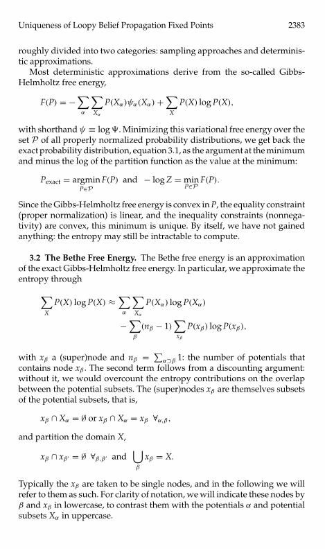
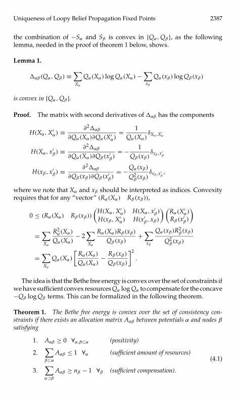
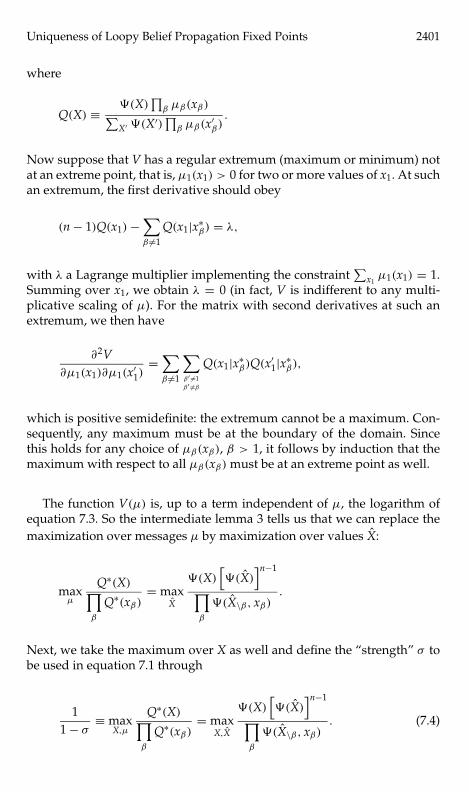
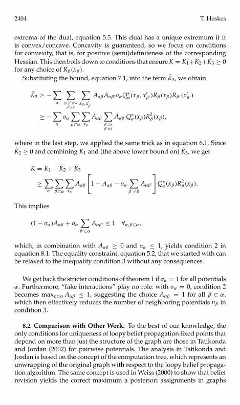
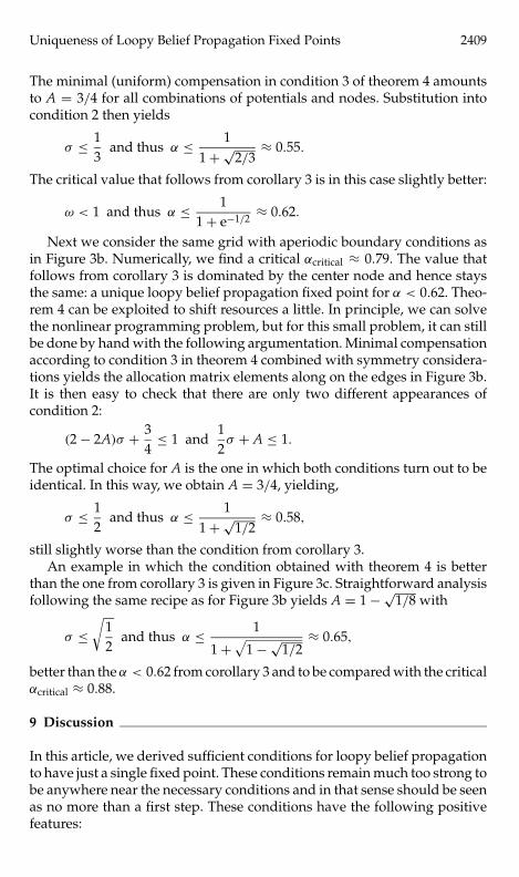
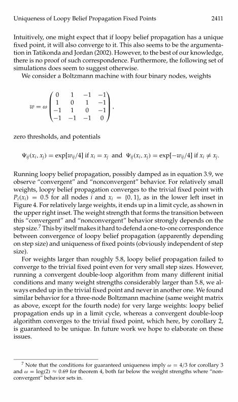
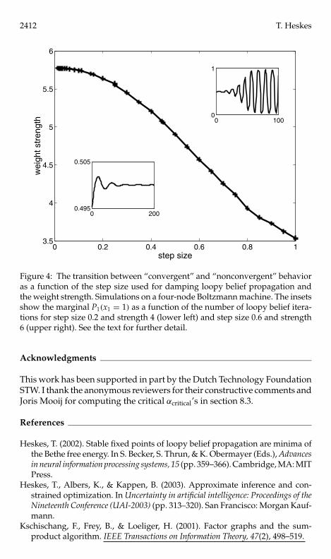2380 T Heskes

conditions for uniqueness Such conditions are not only relevant from a the-oretical point of view but can also be used to derive faster algorithms andsuggest different free energies as will be discussed in section 9

2 Outline

Before getting into the mathematical details we first sketch the line of rea-soning that will be followed in this article It is inspired by the connectionbetween fixed points of loopy belief propagation and extrema of the Bethefree energy by studying the Bethe free energy we can learn about propertiesof loopy belief propagation

The Bethe free energy is an approximation to the exact variational Gibbs-Helmholtz free energy Both are concepts from (statistical) physics Abstract-ing from the physical interpretation the Gibbs-Helmholtz free energy isldquojustrdquo a functional with a unique minimum the argument of which corre-sponds to the exact probability distribution However the Gibbs-Helmholtzfree energy is as intractable as the exact probability distribution The ideais then to approximate the Gibbs-Helmholtz free energy in the hope thatthe minimum of such a tractable approximate free energy relates to theminimum of the exact free energy Examples of such approximations arethe mean-field free energy the Bethe free energy and the Kikuchi free en-ergy The connections between the Gibbs-Helmholtz free energy Bethe freeenergy and loopy belief propagation are reviewed in section 3

The Bethe free energy is a function of so-called pseudomarginals or be-liefs For the minimum of the Bethe free energy to make sense these pseudo-marginals have to be properly normalized as well as consistent Our startingpoint the upper-left corner in Figure 1 is a constrained minimization prob-lem In general it is in fact a nonconvex constrained minimization problemsince the Bethe free energy is a nonconvex function of the pseudomarginals(the constraints are linear in these pseudomarginals)

However using the constraints on the pseudomarginals it may be pos-sible to rewrite the Bethe free energy in a form that is convex in the pseudo-marginals When this is possible we call the Bethe free energy ldquoconvex overthe set of constraintsrdquo (Pakzad amp Anantharam 2002) Now if the Bethe freeenergy is convex over the set of constraints we have in combination withthe linearity of the constraints a convex constrained minimization prob-lem Convex constrained minimization problems have a unique solution(see eg (Luenberger 1984) which explains link d in Figure 1

Sufficient conditions for convexity over the set of constraints link b inFigure 1 can be found in Pakzad and Anantharam (2002) and Heskes et al(2003) They are (re)derived and discussed in section 4 These conditionsdepend on only the structure of the graph not on the (strength of the)potentials that make up the probability distribution defined over this graphA corollary of these conditions derived in section 43 is that the Bethefree energy for a graph with a single loop is ldquojustrdquo convex over the set of





2382 T Heskes







Pexact(X) = 1Z

prodα

α(Xα) (31)



Pexact(Xα) =sumXα

Pexact(X)





F(P) = minussumα

sumXα

P(Xα)ψα(Xα)+sum

X

P(X) log P(X)




F(P)



sumX


sumXα

P(Xα) log P(Xα)

minussumβ

(nβ minus 1)sumxβ

P(xβ) log P(xβ)





xβ = X


2384 T Heskes



sumXα


sumXα


minussumβ

(nβ minus 1)sumxβ



Xα




minQαQβ isinQ

F(QαQβ)




+sumβ

sumαsupβ

sumxβ


]

+sumα

λα

[1minus

sumXα

Qα(Xα)

]

+sumβ

λβ

[1minus

sumβ

Qβ(xβ)

] (34)






[λα minus 1+

sumβsubα

λαβ(xβ)

]


[1

nβ minus 1

1minus λβ +

sumαsupβ

λαβ(xβ)

]






(36)






(38)


2386 T Heskes







minQαQβ

maxλαβ λαλβ












Lemma 1




is convex in QαQβ










Q2β(xβ)

δxβ xprimeβ





)

=sumXα

R2α(Xα)

Qα(Xα)minus 2

sumXα


+sumxβ

Qα(xβ)R2β(xβ)

Q2β(xβ)

=sumXα

Qα(Xα)

[Rα(Xα)


Qβ(xβ)

]2




2sumβsubα


3sumαsupβ


(41)

2388 T Heskes



α

Sα(Qα)minussumβ


]



α

Sα minussumβ

(nβ minus 1)Sβ

]

= minussumα

(1minus

sumβsubα

Aαβ +sumβsubα

Aαβ

)Sα

minussumβ

minussumαsupβ

Aαβ +sumαsupβ


Sβ

= minussumα

(1minus

sumβsubα

Aαβ

)Sα minus

sumα

sumβsubα


minussumβ

[sumαsupβ


]Sβ










sumαsupβ






sumαsupβ





2390 T Heskes




βisinB


1 ge 0 (42)





sumβisinB


sumαsupβ


sumβsubα


1







2392 T Heskes





sumXα


sumXα


minussumβ

sumαsupβ

Aαβ

sumxβ



sumαsupβ




sumXα

Qα(Xα)ψα(Xα)

+sumα

sumXα


minussumα

sumβsubα

Aαβ

sumxβ




+sumβ

sumαsupβ

sumxβ

λαβ(xβ)

times[

1nβ minus 1

sumαprimesupβ


]

+sumα

λα

[1minus

sumXα

Qα(Xα)

]

+sumβ

(nβ minus 1)

[sumxβ

Qβ(xβ)minus 1

] (53)




minQαQβ

maxλαβ λα


maxλαβ λα

minQα


Rewriting

sumβ

sumαsupβ

sumxβ

λαβ(xβ)

[1

nβ minus 1

sumαprimesupβ


]

= minussumα

sumβsubα

sumxβ

λαβ(xβ)Qα(xβ)

with


sumαprimesupβ




[λα minus 1+

sumβsubα


] (54)


2394 T Heskes



= minussumα

sumXα

α(Xα)


sumβsubα


]

+sumα

λα +sumβ

(nβ minus 1)

[sumxβ

Qβ(xβ)minus 1

] (55)



] =sumXα

α(Xα) exp

[sumβsubα


]




= minussumα


(nβ minus 1)

[sumxβ

Qβ(xβ)minus 1

] (57)








yf (x y)



yf (x y)






2396 T Heskes



nβ we then have


logsumXα

α(Xα) exp

[sumβsubα

nβ minus 1nβ

log Qβ(xβ)

]

+sumβ

(nβ minus 1)

[sumxβ

Qβ(xβ)minus 1

]

ge minussumα

sumβsubα

nβ minus 1nβ

logsumXα

α(Xα)Qβ(xβ)

+sumβ

(nβ minus 1)

[sumxβ

Qβ(xβ)minus 1

]

ge minussumα

sumβsubα

nβ minus 1nβ

log

sum

Xαβ

max

+sumβ

(nβ minus 1)

[minus log

sumxβ

Qβ(xβ)+sumxβ

Qβ(xβ)minus 1

]

ge minussumα

sumβsubα

nβ minus 1nβ

log

sum

Xαβ

max


ynβminus1




partGpartQβ(xβ)

= minussumαsupβ

Aαβ


+ (nβ minus 1)





we make use of







δxβ xprimeβ

+sumαsupβ

A2αβ





for β prime = β




sumxβ xβprime



ββ prime

sumxβ xβprime


=sumα

sumβsubα

sumxβ


+sumα

sumββ primesubα

sumxβ xprime

βprime


primeβ prime) (K2)

minussumα


sumxβ xprime

βprime



2398 T Heskes


K2 =sumα

[sumβsubα

sumxβ


]2

ge 0

and5

K3 =sumα


sumxβ xprime

βprime


times

12


]2 minus 12

R2β(xβ)minus

12

R2β prime(x

primeβ prime)

gesumα

sumβsubα

sumxβ

Aαβ

(sumβ primesubα


)Qlowastα(xβ)R

2β(xβ) (61)

we have


sumβsubα

sumxβ

Aαβ

(1minus

sumβ primesubα

Aαβ prime

)Qlowastα(xβ)R

2β(xβ)



Aαβ le 1 forallα









K2 + K3 =sumα

sumβsubα

sumxβ xprime

βprime



primeβ) (K2)

minussumα


sumxβ xprime

βprime

AαβAαβ prime


primeβ prime) (K3)











βprime (71)





sumβsubα

ψα(Xαβ xβ)

] (72)

where nα equivsum

βsubα 1

2400 T Heskes


Qlowast(X)nprodβ=1

Qlowast(xβ)=(X)

prodβ

microβ(xβ)

[sumXprime(Xprime)

prodβ

microβ(xprimeβ)

]nminus1

prodβ

sum

Xprimeβ



=(X)

[sumXprime(Xprime)

prodβ

microβ(xprimeβ)

]nminus1

prodβ

sum

Xprimeβ



(73)




[sumX

(X)nprodβ=1

microβ(xβ)

]

minusnsumβ=1

log

sum

Xβ






partVpartmicro1(x1)


Q(x1|xlowastβ)





where



primeβ)





x1micro1(x1) = 1



=sumβ =1





maxmicro

Qlowast(X)prodβ

Qlowast(xβ)= max

X

(X)[(X)

]nminus1

prodβ

(Xβ xβ)



Xmicro

Qlowast(X)prodβ

Qlowast(xβ)= max

XX

(X)[(X)

]nminus1

prodβ

(Xβ xβ) (74)

2402 T Heskes






W(X X) with


sumβ

ψ(Xβ xβ)

]




if (X) = (X)prodβ

















81 Main Result






3sumαsupβ


(81)



2404 T Heskes



K3 ge minussumα


sumxβ xprime

βprime


ge minussumα

σαsumβsubα

sumxβ

Aαβ




K = K1 + K2 + K3

gesumα

sumβsubα

sumxβ

Aαβ


sumβ prime =β

Aαβ prime

]Qlowastα(xβ)R

2β(xβ)

This implies









Pexact(X) = 1Z

prodα

α(Xα)prodβ

β(xβ)



sumαsupβ

(max

Xα


ψα(Xα)

)lt 2 forallβ (82)







φαβ(xβ)


2406 T Heskes


minφ1φ2

maxx1x2


ψ(x1 x2)

= minφ1φ2

maxx1x2

[ψ(x1 x2)+ φ1(x1)+ φ2(x2)]

minus minx1x2

[ψ(x1 x2)+ φ1(x1)+ φ2(x2)]


ψ(x1 x2)+ φ1(x1)+ φ2(x2) = ψ(x1 x2)+ φ1(x1)+ φ2(x2)



φ1(x1)minus φ1(x1) = 12


]φ2(x2)minus φ2(x2) = 1

2


]



= 12


]


minφ1φ2

maxx1x2


ψ(x1 x2)


2












σα le 1 (86)





)



ω = 2 log[

α

1minus α]


1minus αα

)2

2408 T Heskes



further explanation



σ le 13


asymp 055





12σ + A le 1


σ le 12


asymp 058



σ leradic

12

and thus α le 1

1+radic



9 Discussion


2410 T Heskes














w = ω







2412 T Heskes

0 02 04 06 08 135

4

45

5

55

6

step size

wei

ght s

tren

gth

0 2000495

0505

0 1000

1


Acknowledgments


References


























2382 T Heskes







Pexact(X) = 1Z

prodα

α(Xα) (31)



Pexact(Xα) =sumXα

Pexact(X)





F(P) = minussumα

sumXα

P(Xα)ψα(Xα)+sum

X

P(X) log P(X)




F(P)



sumX


sumXα

P(Xα) log P(Xα)

minussumβ

(nβ minus 1)sumxβ

P(xβ) log P(xβ)





xβ = X


2384 T Heskes



sumXα


sumXα


minussumβ

(nβ minus 1)sumxβ



Xα




minQαQβ isinQ

F(QαQβ)




+sumβ

sumαsupβ

sumxβ


]

+sumα

λα

[1minus

sumXα

Qα(Xα)

]

+sumβ

λβ

[1minus

sumβ

Qβ(xβ)

] (34)






[λα minus 1+

sumβsubα

λαβ(xβ)

]


[1

nβ minus 1

1minus λβ +

sumαsupβ

λαβ(xβ)

]






(36)






(38)


2386 T Heskes







minQαQβ

maxλαβ λαλβ












Lemma 1




is convex in QαQβ










Q2β(xβ)

δxβ xprimeβ





)

=sumXα

R2α(Xα)

Qα(Xα)minus 2

sumXα


+sumxβ

Qα(xβ)R2β(xβ)

Q2β(xβ)

=sumXα

Qα(Xα)

[Rα(Xα)


Qβ(xβ)

]2




2sumβsubα


3sumαsupβ


(41)

2388 T Heskes



α

Sα(Qα)minussumβ


]



α

Sα minussumβ

(nβ minus 1)Sβ

]

= minussumα

(1minus

sumβsubα

Aαβ +sumβsubα

Aαβ

)Sα

minussumβ

minussumαsupβ

Aαβ +sumαsupβ


Sβ

= minussumα

(1minus

sumβsubα

Aαβ

)Sα minus

sumα

sumβsubα


minussumβ

[sumαsupβ


]Sβ










sumαsupβ






sumαsupβ





2390 T Heskes




βisinB


1 ge 0 (42)





sumβisinB


sumαsupβ


sumβsubα


1







2392 T Heskes





sumXα


sumXα


minussumβ

sumαsupβ

Aαβ

sumxβ



sumαsupβ




sumXα

Qα(Xα)ψα(Xα)

+sumα

sumXα


minussumα

sumβsubα

Aαβ

sumxβ




+sumβ

sumαsupβ

sumxβ

λαβ(xβ)

times[

1nβ minus 1

sumαprimesupβ


]

+sumα

λα

[1minus

sumXα

Qα(Xα)

]

+sumβ

(nβ minus 1)

[sumxβ

Qβ(xβ)minus 1

] (53)




minQαQβ

maxλαβ λα


maxλαβ λα

minQα


Rewriting

sumβ

sumαsupβ

sumxβ

λαβ(xβ)

[1

nβ minus 1

sumαprimesupβ


]

= minussumα

sumβsubα

sumxβ

λαβ(xβ)Qα(xβ)

with


sumαprimesupβ




[λα minus 1+

sumβsubα


] (54)


2394 T Heskes



= minussumα

sumXα

α(Xα)


sumβsubα


]

+sumα

λα +sumβ

(nβ minus 1)

[sumxβ

Qβ(xβ)minus 1

] (55)



] =sumXα

α(Xα) exp

[sumβsubα


]




= minussumα


(nβ minus 1)

[sumxβ

Qβ(xβ)minus 1

] (57)








yf (x y)



yf (x y)






2396 T Heskes



nβ we then have


logsumXα

α(Xα) exp

[sumβsubα

nβ minus 1nβ

log Qβ(xβ)

]

+sumβ

(nβ minus 1)

[sumxβ

Qβ(xβ)minus 1

]

ge minussumα

sumβsubα

nβ minus 1nβ

logsumXα

α(Xα)Qβ(xβ)

+sumβ

(nβ minus 1)

[sumxβ

Qβ(xβ)minus 1

]

ge minussumα

sumβsubα

nβ minus 1nβ

log

sum

Xαβ

max

+sumβ

(nβ minus 1)

[minus log

sumxβ

Qβ(xβ)+sumxβ

Qβ(xβ)minus 1

]

ge minussumα

sumβsubα

nβ minus 1nβ

log

sum

Xαβ

max


ynβminus1




partGpartQβ(xβ)

= minussumαsupβ

Aαβ


+ (nβ minus 1)





we make use of







δxβ xprimeβ

+sumαsupβ

A2αβ





for β prime = β




sumxβ xβprime



ββ prime

sumxβ xβprime


=sumα

sumβsubα

sumxβ


+sumα

sumββ primesubα

sumxβ xprime

βprime


primeβ prime) (K2)

minussumα


sumxβ xprime

βprime



2398 T Heskes


K2 =sumα

[sumβsubα

sumxβ


]2

ge 0

and5

K3 =sumα


sumxβ xprime

βprime


times

12


]2 minus 12

R2β(xβ)minus

12

R2β prime(x

primeβ prime)

gesumα

sumβsubα

sumxβ

Aαβ

(sumβ primesubα


)Qlowastα(xβ)R

2β(xβ) (61)

we have


sumβsubα

sumxβ

Aαβ

(1minus

sumβ primesubα

Aαβ prime

)Qlowastα(xβ)R

2β(xβ)



Aαβ le 1 forallα









K2 + K3 =sumα

sumβsubα

sumxβ xprime

βprime



primeβ) (K2)

minussumα


sumxβ xprime

βprime

AαβAαβ prime


primeβ prime) (K3)











βprime (71)





sumβsubα

ψα(Xαβ xβ)

] (72)

where nα equivsum

βsubα 1

2400 T Heskes


Qlowast(X)nprodβ=1

Qlowast(xβ)=(X)

prodβ

microβ(xβ)

[sumXprime(Xprime)

prodβ

microβ(xprimeβ)

]nminus1

prodβ

sum

Xprimeβ



=(X)

[sumXprime(Xprime)

prodβ

microβ(xprimeβ)

]nminus1

prodβ

sum

Xprimeβ



(73)




[sumX

(X)nprodβ=1

microβ(xβ)

]

minusnsumβ=1

log

sum

Xβ






partVpartmicro1(x1)


Q(x1|xlowastβ)





where



primeβ)





x1micro1(x1) = 1



=sumβ =1





maxmicro

Qlowast(X)prodβ

Qlowast(xβ)= max

X

(X)[(X)

]nminus1

prodβ

(Xβ xβ)



Xmicro

Qlowast(X)prodβ

Qlowast(xβ)= max

XX

(X)[(X)

]nminus1

prodβ

(Xβ xβ) (74)

2402 T Heskes






W(X X) with


sumβ

ψ(Xβ xβ)

]




if (X) = (X)prodβ

















81 Main Result






3sumαsupβ


(81)



2404 T Heskes



K3 ge minussumα


sumxβ xprime

βprime


ge minussumα

σαsumβsubα

sumxβ

Aαβ




K = K1 + K2 + K3

gesumα

sumβsubα

sumxβ

Aαβ


sumβ prime =β

Aαβ prime

]Qlowastα(xβ)R

2β(xβ)

This implies









Pexact(X) = 1Z

prodα

α(Xα)prodβ

β(xβ)



sumαsupβ

(max

Xα


ψα(Xα)

)lt 2 forallβ (82)







φαβ(xβ)


2406 T Heskes


minφ1φ2

maxx1x2


ψ(x1 x2)

= minφ1φ2

maxx1x2

[ψ(x1 x2)+ φ1(x1)+ φ2(x2)]

minus minx1x2

[ψ(x1 x2)+ φ1(x1)+ φ2(x2)]


ψ(x1 x2)+ φ1(x1)+ φ2(x2) = ψ(x1 x2)+ φ1(x1)+ φ2(x2)



φ1(x1)minus φ1(x1) = 12


]φ2(x2)minus φ2(x2) = 1

2


]



= 12


]


minφ1φ2

maxx1x2


ψ(x1 x2)


2












σα le 1 (86)





)



ω = 2 log[

α

1minus α]


1minus αα

)2

2408 T Heskes



further explanation



σ le 13


asymp 055





12σ + A le 1


σ le 12


asymp 058



σ leradic

12

and thus α le 1

1+radic



9 Discussion


2410 T Heskes














w = ω







2412 T Heskes

0 02 04 06 08 135

4

45

5

55

6

step size

wei

ght s

tren

gth

0 2000495

0505

0 1000

1


Acknowledgments


References






















2382 T Heskes







Pexact(X) = 1Z

prodα

α(Xα) (31)



Pexact(Xα) =sumXα

Pexact(X)





F(P) = minussumα

sumXα

P(Xα)ψα(Xα)+sum

X

P(X) log P(X)




F(P)



sumX


sumXα

P(Xα) log P(Xα)

minussumβ

(nβ minus 1)sumxβ

P(xβ) log P(xβ)





xβ = X


2384 T Heskes



sumXα


sumXα


minussumβ

(nβ minus 1)sumxβ



Xα




minQαQβ isinQ

F(QαQβ)




+sumβ

sumαsupβ

sumxβ


]

+sumα

λα

[1minus

sumXα

Qα(Xα)

]

+sumβ

λβ

[1minus

sumβ

Qβ(xβ)

] (34)






[λα minus 1+

sumβsubα

λαβ(xβ)

]


[1

nβ minus 1

1minus λβ +

sumαsupβ

λαβ(xβ)

]






(36)






(38)


2386 T Heskes







minQαQβ

maxλαβ λαλβ












Lemma 1




is convex in QαQβ










Q2β(xβ)

δxβ xprimeβ





)

=sumXα

R2α(Xα)

Qα(Xα)minus 2

sumXα


+sumxβ

Qα(xβ)R2β(xβ)

Q2β(xβ)

=sumXα

Qα(Xα)

[Rα(Xα)


Qβ(xβ)

]2




2sumβsubα


3sumαsupβ


(41)

2388 T Heskes



α

Sα(Qα)minussumβ


]



α

Sα minussumβ

(nβ minus 1)Sβ

]

= minussumα

(1minus

sumβsubα

Aαβ +sumβsubα

Aαβ

)Sα

minussumβ

minussumαsupβ

Aαβ +sumαsupβ


Sβ

= minussumα

(1minus

sumβsubα

Aαβ

)Sα minus

sumα

sumβsubα


minussumβ

[sumαsupβ


]Sβ










sumαsupβ






sumαsupβ





2390 T Heskes




βisinB


1 ge 0 (42)





sumβisinB


sumαsupβ


sumβsubα


1







2392 T Heskes





sumXα


sumXα


minussumβ

sumαsupβ

Aαβ

sumxβ



sumαsupβ




sumXα

Qα(Xα)ψα(Xα)

+sumα

sumXα


minussumα

sumβsubα

Aαβ

sumxβ




+sumβ

sumαsupβ

sumxβ

λαβ(xβ)

times[

1nβ minus 1

sumαprimesupβ


]

+sumα

λα

[1minus

sumXα

Qα(Xα)

]

+sumβ

(nβ minus 1)

[sumxβ

Qβ(xβ)minus 1

] (53)




minQαQβ

maxλαβ λα


maxλαβ λα

minQα


Rewriting

sumβ

sumαsupβ

sumxβ

λαβ(xβ)

[1

nβ minus 1

sumαprimesupβ


]

= minussumα

sumβsubα

sumxβ

λαβ(xβ)Qα(xβ)

with


sumαprimesupβ




[λα minus 1+

sumβsubα


] (54)


2394 T Heskes



= minussumα

sumXα

α(Xα)


sumβsubα


]

+sumα

λα +sumβ

(nβ minus 1)

[sumxβ

Qβ(xβ)minus 1

] (55)



] =sumXα

α(Xα) exp

[sumβsubα


]




= minussumα


(nβ minus 1)

[sumxβ

Qβ(xβ)minus 1

] (57)








yf (x y)



yf (x y)






2396 T Heskes



nβ we then have


logsumXα

α(Xα) exp

[sumβsubα

nβ minus 1nβ

log Qβ(xβ)

]

+sumβ

(nβ minus 1)

[sumxβ

Qβ(xβ)minus 1

]

ge minussumα

sumβsubα

nβ minus 1nβ

logsumXα

α(Xα)Qβ(xβ)

+sumβ

(nβ minus 1)

[sumxβ

Qβ(xβ)minus 1

]

ge minussumα

sumβsubα

nβ minus 1nβ

log

sum

Xαβ

max

+sumβ

(nβ minus 1)

[minus log

sumxβ

Qβ(xβ)+sumxβ

Qβ(xβ)minus 1

]

ge minussumα

sumβsubα

nβ minus 1nβ

log

sum

Xαβ

max


ynβminus1




partGpartQβ(xβ)

= minussumαsupβ

Aαβ


+ (nβ minus 1)





we make use of







δxβ xprimeβ

+sumαsupβ

A2αβ





for β prime = β




sumxβ xβprime



ββ prime

sumxβ xβprime


=sumα

sumβsubα

sumxβ


+sumα

sumββ primesubα

sumxβ xprime

βprime


primeβ prime) (K2)

minussumα


sumxβ xprime

βprime



2398 T Heskes


K2 =sumα

[sumβsubα

sumxβ


]2

ge 0

and5

K3 =sumα


sumxβ xprime

βprime


times

12


]2 minus 12

R2β(xβ)minus

12

R2β prime(x

primeβ prime)

gesumα

sumβsubα

sumxβ

Aαβ

(sumβ primesubα


)Qlowastα(xβ)R

2β(xβ) (61)

we have


sumβsubα

sumxβ

Aαβ

(1minus

sumβ primesubα

Aαβ prime

)Qlowastα(xβ)R

2β(xβ)



Aαβ le 1 forallα









K2 + K3 =sumα

sumβsubα

sumxβ xprime

βprime



primeβ) (K2)

minussumα


sumxβ xprime

βprime

AαβAαβ prime


primeβ prime) (K3)











βprime (71)





sumβsubα

ψα(Xαβ xβ)

] (72)

where nα equivsum

βsubα 1

2400 T Heskes


Qlowast(X)nprodβ=1

Qlowast(xβ)=(X)

prodβ

microβ(xβ)

[sumXprime(Xprime)

prodβ

microβ(xprimeβ)

]nminus1

prodβ

sum

Xprimeβ



=(X)

[sumXprime(Xprime)

prodβ

microβ(xprimeβ)

]nminus1

prodβ

sum

Xprimeβ



(73)




[sumX

(X)nprodβ=1

microβ(xβ)

]

minusnsumβ=1

log

sum

Xβ






partVpartmicro1(x1)


Q(x1|xlowastβ)





where



primeβ)





x1micro1(x1) = 1



=sumβ =1





maxmicro

Qlowast(X)prodβ

Qlowast(xβ)= max

X

(X)[(X)

]nminus1

prodβ

(Xβ xβ)



Xmicro

Qlowast(X)prodβ

Qlowast(xβ)= max

XX

(X)[(X)

]nminus1

prodβ

(Xβ xβ) (74)

2402 T Heskes






W(X X) with


sumβ

ψ(Xβ xβ)

]




if (X) = (X)prodβ

















81 Main Result






3sumαsupβ


(81)



2404 T Heskes



K3 ge minussumα


sumxβ xprime

βprime


ge minussumα

σαsumβsubα

sumxβ

Aαβ




K = K1 + K2 + K3

gesumα

sumβsubα

sumxβ

Aαβ


sumβ prime =β

Aαβ prime

]Qlowastα(xβ)R

2β(xβ)

This implies









Pexact(X) = 1Z

prodα

α(Xα)prodβ

β(xβ)



sumαsupβ

(max

Xα


ψα(Xα)

)lt 2 forallβ (82)







φαβ(xβ)


2406 T Heskes


minφ1φ2

maxx1x2


ψ(x1 x2)

= minφ1φ2

maxx1x2

[ψ(x1 x2)+ φ1(x1)+ φ2(x2)]

minus minx1x2

[ψ(x1 x2)+ φ1(x1)+ φ2(x2)]


ψ(x1 x2)+ φ1(x1)+ φ2(x2) = ψ(x1 x2)+ φ1(x1)+ φ2(x2)



φ1(x1)minus φ1(x1) = 12


]φ2(x2)minus φ2(x2) = 1

2


]



= 12


]


minφ1φ2

maxx1x2


ψ(x1 x2)


2












σα le 1 (86)





)



ω = 2 log[

α

1minus α]


1minus αα

)2

2408 T Heskes



further explanation



σ le 13


asymp 055





12σ + A le 1


σ le 12


asymp 058



σ leradic

12

and thus α le 1

1+radic



9 Discussion


2410 T Heskes














w = ω







2412 T Heskes

0 02 04 06 08 135

4

45

5

55

6

step size

wei

ght s

tren

gth

0 2000495

0505

0 1000

1


Acknowledgments


References

























F(P) = minussumα

sumXα

P(Xα)ψα(Xα)+sum

X

P(X) log P(X)




F(P)



sumX


sumXα

P(Xα) log P(Xα)

minussumβ

(nβ minus 1)sumxβ

P(xβ) log P(xβ)





xβ = X


2384 T Heskes



sumXα


sumXα


minussumβ

(nβ minus 1)sumxβ



Xα




minQαQβ isinQ

F(QαQβ)




+sumβ

sumαsupβ

sumxβ


]

+sumα

λα

[1minus

sumXα

Qα(Xα)

]

+sumβ

λβ

[1minus

sumβ

Qβ(xβ)

] (34)






[λα minus 1+

sumβsubα

λαβ(xβ)

]


[1

nβ minus 1

1minus λβ +

sumαsupβ

λαβ(xβ)

]






(36)






(38)


2386 T Heskes







minQαQβ

maxλαβ λαλβ












Lemma 1




is convex in QαQβ










Q2β(xβ)

δxβ xprimeβ





)

=sumXα

R2α(Xα)

Qα(Xα)minus 2

sumXα


+sumxβ

Qα(xβ)R2β(xβ)

Q2β(xβ)

=sumXα

Qα(Xα)

[Rα(Xα)


Qβ(xβ)

]2




2sumβsubα


3sumαsupβ


(41)

2388 T Heskes



α

Sα(Qα)minussumβ


]



α

Sα minussumβ

(nβ minus 1)Sβ

]

= minussumα

(1minus

sumβsubα

Aαβ +sumβsubα

Aαβ

)Sα

minussumβ

minussumαsupβ

Aαβ +sumαsupβ


Sβ

= minussumα

(1minus

sumβsubα

Aαβ

)Sα minus

sumα

sumβsubα


minussumβ

[sumαsupβ


]Sβ










sumαsupβ






sumαsupβ





2390 T Heskes




βisinB


1 ge 0 (42)





sumβisinB


sumαsupβ


sumβsubα


1







2392 T Heskes





sumXα


sumXα


minussumβ

sumαsupβ

Aαβ

sumxβ



sumαsupβ




sumXα

Qα(Xα)ψα(Xα)

+sumα

sumXα


minussumα

sumβsubα

Aαβ

sumxβ




+sumβ

sumαsupβ

sumxβ

λαβ(xβ)

times[

1nβ minus 1

sumαprimesupβ


]

+sumα

λα

[1minus

sumXα

Qα(Xα)

]

+sumβ

(nβ minus 1)

[sumxβ

Qβ(xβ)minus 1

] (53)




minQαQβ

maxλαβ λα


maxλαβ λα

minQα


Rewriting

sumβ

sumαsupβ

sumxβ

λαβ(xβ)

[1

nβ minus 1

sumαprimesupβ


]

= minussumα

sumβsubα

sumxβ

λαβ(xβ)Qα(xβ)

with


sumαprimesupβ




[λα minus 1+

sumβsubα


] (54)


2394 T Heskes



= minussumα

sumXα

α(Xα)


sumβsubα


]

+sumα

λα +sumβ

(nβ minus 1)

[sumxβ

Qβ(xβ)minus 1

] (55)



] =sumXα

α(Xα) exp

[sumβsubα


]




= minussumα


(nβ minus 1)

[sumxβ

Qβ(xβ)minus 1

] (57)








yf (x y)



yf (x y)






2396 T Heskes



nβ we then have


logsumXα

α(Xα) exp

[sumβsubα

nβ minus 1nβ

log Qβ(xβ)

]

+sumβ

(nβ minus 1)

[sumxβ

Qβ(xβ)minus 1

]

ge minussumα

sumβsubα

nβ minus 1nβ

logsumXα

α(Xα)Qβ(xβ)

+sumβ

(nβ minus 1)

[sumxβ

Qβ(xβ)minus 1

]

ge minussumα

sumβsubα

nβ minus 1nβ

log

sum

Xαβ

max

+sumβ

(nβ minus 1)

[minus log

sumxβ

Qβ(xβ)+sumxβ

Qβ(xβ)minus 1

]

ge minussumα

sumβsubα

nβ minus 1nβ

log

sum

Xαβ

max


ynβminus1




partGpartQβ(xβ)

= minussumαsupβ

Aαβ


+ (nβ minus 1)





we make use of







δxβ xprimeβ

+sumαsupβ

A2αβ





for β prime = β




sumxβ xβprime



ββ prime

sumxβ xβprime


=sumα

sumβsubα

sumxβ


+sumα

sumββ primesubα

sumxβ xprime

βprime


primeβ prime) (K2)

minussumα


sumxβ xprime

βprime



2398 T Heskes


K2 =sumα

[sumβsubα

sumxβ


]2

ge 0

and5

K3 =sumα


sumxβ xprime

βprime


times

12


]2 minus 12

R2β(xβ)minus

12

R2β prime(x

primeβ prime)

gesumα

sumβsubα

sumxβ

Aαβ

(sumβ primesubα


)Qlowastα(xβ)R

2β(xβ) (61)

we have


sumβsubα

sumxβ

Aαβ

(1minus

sumβ primesubα

Aαβ prime

)Qlowastα(xβ)R

2β(xβ)



Aαβ le 1 forallα









K2 + K3 =sumα

sumβsubα

sumxβ xprime

βprime



primeβ) (K2)

minussumα


sumxβ xprime

βprime

AαβAαβ prime


primeβ prime) (K3)











βprime (71)





sumβsubα

ψα(Xαβ xβ)

] (72)

where nα equivsum

βsubα 1

2400 T Heskes


Qlowast(X)nprodβ=1

Qlowast(xβ)=(X)

prodβ

microβ(xβ)

[sumXprime(Xprime)

prodβ

microβ(xprimeβ)

]nminus1

prodβ

sum

Xprimeβ



=(X)

[sumXprime(Xprime)

prodβ

microβ(xprimeβ)

]nminus1

prodβ

sum

Xprimeβ



(73)




[sumX

(X)nprodβ=1

microβ(xβ)

]

minusnsumβ=1

log

sum

Xβ






partVpartmicro1(x1)


Q(x1|xlowastβ)





where



primeβ)





x1micro1(x1) = 1



=sumβ =1





maxmicro

Qlowast(X)prodβ

Qlowast(xβ)= max

X

(X)[(X)

]nminus1

prodβ

(Xβ xβ)



Xmicro

Qlowast(X)prodβ

Qlowast(xβ)= max

XX

(X)[(X)

]nminus1

prodβ

(Xβ xβ) (74)

2402 T Heskes






W(X X) with


sumβ

ψ(Xβ xβ)

]




if (X) = (X)prodβ

















81 Main Result






3sumαsupβ


(81)



2404 T Heskes



K3 ge minussumα


sumxβ xprime

βprime


ge minussumα

σαsumβsubα

sumxβ

Aαβ




K = K1 + K2 + K3

gesumα

sumβsubα

sumxβ

Aαβ


sumβ prime =β

Aαβ prime

]Qlowastα(xβ)R

2β(xβ)

This implies









Pexact(X) = 1Z

prodα

α(Xα)prodβ

β(xβ)



sumαsupβ

(max

Xα


ψα(Xα)

)lt 2 forallβ (82)







φαβ(xβ)


2406 T Heskes


minφ1φ2

maxx1x2


ψ(x1 x2)

= minφ1φ2

maxx1x2

[ψ(x1 x2)+ φ1(x1)+ φ2(x2)]

minus minx1x2

[ψ(x1 x2)+ φ1(x1)+ φ2(x2)]


ψ(x1 x2)+ φ1(x1)+ φ2(x2) = ψ(x1 x2)+ φ1(x1)+ φ2(x2)



φ1(x1)minus φ1(x1) = 12


]φ2(x2)minus φ2(x2) = 1

2


]



= 12


]


minφ1φ2

maxx1x2


ψ(x1 x2)


2












σα le 1 (86)





)



ω = 2 log[

α

1minus α]


1minus αα

)2

2408 T Heskes



further explanation



σ le 13


asymp 055





12σ + A le 1


σ le 12


asymp 058



σ leradic

12

and thus α le 1

1+radic



9 Discussion


2410 T Heskes














w = ω







2412 T Heskes

0 02 04 06 08 135

4

45

5

55

6

step size

wei

ght s

tren

gth

0 2000495

0505

0 1000

1


Acknowledgments


References






















2384 T Heskes



sumXα


sumXα


minussumβ

(nβ minus 1)sumxβ



Xα




minQαQβ isinQ

F(QαQβ)




+sumβ

sumαsupβ

sumxβ


]

+sumα

λα

[1minus

sumXα

Qα(Xα)

]

+sumβ

λβ

[1minus

sumβ

Qβ(xβ)

] (34)






[λα minus 1+

sumβsubα

λαβ(xβ)

]


[1

nβ minus 1

1minus λβ +

sumαsupβ

λαβ(xβ)

]






(36)






(38)


2386 T Heskes







minQαQβ

maxλαβ λαλβ












Lemma 1




is convex in QαQβ










Q2β(xβ)

δxβ xprimeβ





)

=sumXα

R2α(Xα)

Qα(Xα)minus 2

sumXα


+sumxβ

Qα(xβ)R2β(xβ)

Q2β(xβ)

=sumXα

Qα(Xα)

[Rα(Xα)


Qβ(xβ)

]2




2sumβsubα


3sumαsupβ


(41)

2388 T Heskes



α

Sα(Qα)minussumβ


]



α

Sα minussumβ

(nβ minus 1)Sβ

]

= minussumα

(1minus

sumβsubα

Aαβ +sumβsubα

Aαβ

)Sα

minussumβ

minussumαsupβ

Aαβ +sumαsupβ


Sβ

= minussumα

(1minus

sumβsubα

Aαβ

)Sα minus

sumα

sumβsubα


minussumβ

[sumαsupβ


]Sβ










sumαsupβ






sumαsupβ





2390 T Heskes




βisinB


1 ge 0 (42)





sumβisinB


sumαsupβ


sumβsubα


1







2392 T Heskes





sumXα


sumXα


minussumβ

sumαsupβ

Aαβ

sumxβ



sumαsupβ




sumXα

Qα(Xα)ψα(Xα)

+sumα

sumXα


minussumα

sumβsubα

Aαβ

sumxβ




+sumβ

sumαsupβ

sumxβ

λαβ(xβ)

times[

1nβ minus 1

sumαprimesupβ


]

+sumα

λα

[1minus

sumXα

Qα(Xα)

]

+sumβ

(nβ minus 1)

[sumxβ

Qβ(xβ)minus 1

] (53)




minQαQβ

maxλαβ λα


maxλαβ λα

minQα


Rewriting

sumβ

sumαsupβ

sumxβ

λαβ(xβ)

[1

nβ minus 1

sumαprimesupβ


]

= minussumα

sumβsubα

sumxβ

λαβ(xβ)Qα(xβ)

with


sumαprimesupβ




[λα minus 1+

sumβsubα


] (54)


2394 T Heskes



= minussumα

sumXα

α(Xα)


sumβsubα


]

+sumα

λα +sumβ

(nβ minus 1)

[sumxβ

Qβ(xβ)minus 1

] (55)



] =sumXα

α(Xα) exp

[sumβsubα


]




= minussumα


(nβ minus 1)

[sumxβ

Qβ(xβ)minus 1

] (57)








yf (x y)



yf (x y)






2396 T Heskes



nβ we then have


logsumXα

α(Xα) exp

[sumβsubα

nβ minus 1nβ

log Qβ(xβ)

]

+sumβ

(nβ minus 1)

[sumxβ

Qβ(xβ)minus 1

]

ge minussumα

sumβsubα

nβ minus 1nβ

logsumXα

α(Xα)Qβ(xβ)

+sumβ

(nβ minus 1)

[sumxβ

Qβ(xβ)minus 1

]

ge minussumα

sumβsubα

nβ minus 1nβ

log

sum

Xαβ

max

+sumβ

(nβ minus 1)

[minus log

sumxβ

Qβ(xβ)+sumxβ

Qβ(xβ)minus 1

]

ge minussumα

sumβsubα

nβ minus 1nβ

log

sum

Xαβ

max


ynβminus1




partGpartQβ(xβ)

= minussumαsupβ

Aαβ


+ (nβ minus 1)





we make use of







δxβ xprimeβ

+sumαsupβ

A2αβ





for β prime = β




sumxβ xβprime



ββ prime

sumxβ xβprime


=sumα

sumβsubα

sumxβ


+sumα

sumββ primesubα

sumxβ xprime

βprime


primeβ prime) (K2)

minussumα


sumxβ xprime

βprime



2398 T Heskes


K2 =sumα

[sumβsubα

sumxβ


]2

ge 0

and5

K3 =sumα


sumxβ xprime

βprime


times

12


]2 minus 12

R2β(xβ)minus

12

R2β prime(x

primeβ prime)

gesumα

sumβsubα

sumxβ

Aαβ

(sumβ primesubα


)Qlowastα(xβ)R

2β(xβ) (61)

we have


sumβsubα

sumxβ

Aαβ

(1minus

sumβ primesubα

Aαβ prime

)Qlowastα(xβ)R

2β(xβ)



Aαβ le 1 forallα









K2 + K3 =sumα

sumβsubα

sumxβ xprime

βprime



primeβ) (K2)

minussumα


sumxβ xprime

βprime

AαβAαβ prime


primeβ prime) (K3)











βprime (71)





sumβsubα

ψα(Xαβ xβ)

] (72)

where nα equivsum

βsubα 1

2400 T Heskes


Qlowast(X)nprodβ=1

Qlowast(xβ)=(X)

prodβ

microβ(xβ)

[sumXprime(Xprime)

prodβ

microβ(xprimeβ)

]nminus1

prodβ

sum

Xprimeβ



=(X)

[sumXprime(Xprime)

prodβ

microβ(xprimeβ)

]nminus1

prodβ

sum

Xprimeβ



(73)




[sumX

(X)nprodβ=1

microβ(xβ)

]

minusnsumβ=1

log

sum

Xβ






partVpartmicro1(x1)


Q(x1|xlowastβ)





where



primeβ)





x1micro1(x1) = 1



=sumβ =1





maxmicro

Qlowast(X)prodβ

Qlowast(xβ)= max

X

(X)[(X)

]nminus1

prodβ

(Xβ xβ)



Xmicro

Qlowast(X)prodβ

Qlowast(xβ)= max

XX

(X)[(X)

]nminus1

prodβ

(Xβ xβ) (74)

2402 T Heskes






W(X X) with


sumβ

ψ(Xβ xβ)

]




if (X) = (X)prodβ

















81 Main Result






3sumαsupβ


(81)



2404 T Heskes



K3 ge minussumα


sumxβ xprime

βprime


ge minussumα

σαsumβsubα

sumxβ

Aαβ




K = K1 + K2 + K3

gesumα

sumβsubα

sumxβ

Aαβ


sumβ prime =β

Aαβ prime

]Qlowastα(xβ)R

2β(xβ)

This implies









Pexact(X) = 1Z

prodα

α(Xα)prodβ

β(xβ)



sumαsupβ

(max

Xα


ψα(Xα)

)lt 2 forallβ (82)







φαβ(xβ)


2406 T Heskes


minφ1φ2

maxx1x2


ψ(x1 x2)

= minφ1φ2

maxx1x2

[ψ(x1 x2)+ φ1(x1)+ φ2(x2)]

minus minx1x2

[ψ(x1 x2)+ φ1(x1)+ φ2(x2)]


ψ(x1 x2)+ φ1(x1)+ φ2(x2) = ψ(x1 x2)+ φ1(x1)+ φ2(x2)



φ1(x1)minus φ1(x1) = 12


]φ2(x2)minus φ2(x2) = 1

2


]



= 12


]


minφ1φ2

maxx1x2


ψ(x1 x2)


2












σα le 1 (86)





)



ω = 2 log[

α

1minus α]


1minus αα

)2

2408 T Heskes



further explanation



σ le 13


asymp 055





12σ + A le 1


σ le 12


asymp 058



σ leradic

12

and thus α le 1

1+radic



9 Discussion


2410 T Heskes














w = ω







2412 T Heskes

0 02 04 06 08 135

4

45

5

55

6

step size

wei

ght s

tren

gth

0 2000495

0505

0 1000

1


Acknowledgments


References

























[λα minus 1+

sumβsubα

λαβ(xβ)

]


[1

nβ minus 1

1minus λβ +

sumαsupβ

λαβ(xβ)

]






(36)






(38)


2386 T Heskes







minQαQβ

maxλαβ λαλβ












Lemma 1




is convex in QαQβ










Q2β(xβ)

δxβ xprimeβ





)

=sumXα

R2α(Xα)

Qα(Xα)minus 2

sumXα


+sumxβ

Qα(xβ)R2β(xβ)

Q2β(xβ)

=sumXα

Qα(Xα)

[Rα(Xα)


Qβ(xβ)

]2




2sumβsubα


3sumαsupβ


(41)

2388 T Heskes



α

Sα(Qα)minussumβ


]



α

Sα minussumβ

(nβ minus 1)Sβ

]

= minussumα

(1minus

sumβsubα

Aαβ +sumβsubα

Aαβ

)Sα

minussumβ

minussumαsupβ

Aαβ +sumαsupβ


Sβ

= minussumα

(1minus

sumβsubα

Aαβ

)Sα minus

sumα

sumβsubα


minussumβ

[sumαsupβ


]Sβ










sumαsupβ






sumαsupβ





2390 T Heskes




βisinB


1 ge 0 (42)





sumβisinB


sumαsupβ


sumβsubα


1







2392 T Heskes





sumXα


sumXα


minussumβ

sumαsupβ

Aαβ

sumxβ



sumαsupβ




sumXα

Qα(Xα)ψα(Xα)

+sumα

sumXα


minussumα

sumβsubα

Aαβ

sumxβ




+sumβ

sumαsupβ

sumxβ

λαβ(xβ)

times[

1nβ minus 1

sumαprimesupβ


]

+sumα

λα

[1minus

sumXα

Qα(Xα)

]

+sumβ

(nβ minus 1)

[sumxβ

Qβ(xβ)minus 1

] (53)




minQαQβ

maxλαβ λα


maxλαβ λα

minQα


Rewriting

sumβ

sumαsupβ

sumxβ

λαβ(xβ)

[1

nβ minus 1

sumαprimesupβ


]

= minussumα

sumβsubα

sumxβ

λαβ(xβ)Qα(xβ)

with


sumαprimesupβ




[λα minus 1+

sumβsubα


] (54)


2394 T Heskes



= minussumα

sumXα

α(Xα)


sumβsubα


]

+sumα

λα +sumβ

(nβ minus 1)

[sumxβ

Qβ(xβ)minus 1

] (55)



] =sumXα

α(Xα) exp

[sumβsubα


]




= minussumα


(nβ minus 1)

[sumxβ

Qβ(xβ)minus 1

] (57)








yf (x y)



yf (x y)






2396 T Heskes



nβ we then have


logsumXα

α(Xα) exp

[sumβsubα

nβ minus 1nβ

log Qβ(xβ)

]

+sumβ

(nβ minus 1)

[sumxβ

Qβ(xβ)minus 1

]

ge minussumα

sumβsubα

nβ minus 1nβ

logsumXα

α(Xα)Qβ(xβ)

+sumβ

(nβ minus 1)

[sumxβ

Qβ(xβ)minus 1

]

ge minussumα

sumβsubα

nβ minus 1nβ

log

sum

Xαβ

max

+sumβ

(nβ minus 1)

[minus log

sumxβ

Qβ(xβ)+sumxβ

Qβ(xβ)minus 1

]

ge minussumα

sumβsubα

nβ minus 1nβ

log

sum

Xαβ

max


ynβminus1




partGpartQβ(xβ)

= minussumαsupβ

Aαβ


+ (nβ minus 1)





we make use of







δxβ xprimeβ

+sumαsupβ

A2αβ





for β prime = β




sumxβ xβprime



ββ prime

sumxβ xβprime


=sumα

sumβsubα

sumxβ


+sumα

sumββ primesubα

sumxβ xprime

βprime


primeβ prime) (K2)

minussumα


sumxβ xprime

βprime



2398 T Heskes


K2 =sumα

[sumβsubα

sumxβ


]2

ge 0

and5

K3 =sumα


sumxβ xprime

βprime


times

12


]2 minus 12

R2β(xβ)minus

12

R2β prime(x

primeβ prime)

gesumα

sumβsubα

sumxβ

Aαβ

(sumβ primesubα


)Qlowastα(xβ)R

2β(xβ) (61)

we have


sumβsubα

sumxβ

Aαβ

(1minus

sumβ primesubα

Aαβ prime

)Qlowastα(xβ)R

2β(xβ)



Aαβ le 1 forallα









K2 + K3 =sumα

sumβsubα

sumxβ xprime

βprime



primeβ) (K2)

minussumα


sumxβ xprime

βprime

AαβAαβ prime


primeβ prime) (K3)











βprime (71)





sumβsubα

ψα(Xαβ xβ)

] (72)

where nα equivsum

βsubα 1

2400 T Heskes


Qlowast(X)nprodβ=1

Qlowast(xβ)=(X)

prodβ

microβ(xβ)

[sumXprime(Xprime)

prodβ

microβ(xprimeβ)

]nminus1

prodβ

sum

Xprimeβ



=(X)

[sumXprime(Xprime)

prodβ

microβ(xprimeβ)

]nminus1

prodβ

sum

Xprimeβ



(73)




[sumX

(X)nprodβ=1

microβ(xβ)

]

minusnsumβ=1

log

sum

Xβ






partVpartmicro1(x1)


Q(x1|xlowastβ)





where



primeβ)





x1micro1(x1) = 1



=sumβ =1





maxmicro

Qlowast(X)prodβ

Qlowast(xβ)= max

X

(X)[(X)

]nminus1

prodβ

(Xβ xβ)



Xmicro

Qlowast(X)prodβ

Qlowast(xβ)= max

XX

(X)[(X)

]nminus1

prodβ

(Xβ xβ) (74)

2402 T Heskes






W(X X) with


sumβ

ψ(Xβ xβ)

]




if (X) = (X)prodβ

















81 Main Result






3sumαsupβ


(81)



2404 T Heskes



K3 ge minussumα


sumxβ xprime

βprime


ge minussumα

σαsumβsubα

sumxβ

Aαβ




K = K1 + K2 + K3

gesumα

sumβsubα

sumxβ

Aαβ


sumβ prime =β

Aαβ prime

]Qlowastα(xβ)R

2β(xβ)

This implies









Pexact(X) = 1Z

prodα

α(Xα)prodβ

β(xβ)



sumαsupβ

(max

Xα


ψα(Xα)

)lt 2 forallβ (82)







φαβ(xβ)


2406 T Heskes


minφ1φ2

maxx1x2


ψ(x1 x2)

= minφ1φ2

maxx1x2

[ψ(x1 x2)+ φ1(x1)+ φ2(x2)]

minus minx1x2

[ψ(x1 x2)+ φ1(x1)+ φ2(x2)]


ψ(x1 x2)+ φ1(x1)+ φ2(x2) = ψ(x1 x2)+ φ1(x1)+ φ2(x2)



φ1(x1)minus φ1(x1) = 12


]φ2(x2)minus φ2(x2) = 1

2


]



= 12


]


minφ1φ2

maxx1x2


ψ(x1 x2)


2












σα le 1 (86)





)



ω = 2 log[

α

1minus α]


1minus αα

)2

2408 T Heskes



further explanation



σ le 13


asymp 055





12σ + A le 1


σ le 12


asymp 058



σ leradic

12

and thus α le 1

1+radic



9 Discussion


2410 T Heskes














w = ω







2412 T Heskes

0 02 04 06 08 135

4

45

5

55

6

step size

wei

ght s

tren

gth

0 2000495

0505

0 1000

1


Acknowledgments


References






















2386 T Heskes







minQαQβ

maxλαβ λαλβ












Lemma 1




is convex in QαQβ










Q2β(xβ)

δxβ xprimeβ





)

=sumXα

R2α(Xα)

Qα(Xα)minus 2

sumXα


+sumxβ

Qα(xβ)R2β(xβ)

Q2β(xβ)

=sumXα

Qα(Xα)

[Rα(Xα)


Qβ(xβ)

]2




2sumβsubα


3sumαsupβ


(41)

2388 T Heskes



α

Sα(Qα)minussumβ


]



α

Sα minussumβ

(nβ minus 1)Sβ

]

= minussumα

(1minus

sumβsubα

Aαβ +sumβsubα

Aαβ

)Sα

minussumβ

minussumαsupβ

Aαβ +sumαsupβ


Sβ

= minussumα

(1minus

sumβsubα

Aαβ

)Sα minus

sumα

sumβsubα


minussumβ

[sumαsupβ


]Sβ










sumαsupβ






sumαsupβ





2390 T Heskes




βisinB


1 ge 0 (42)





sumβisinB


sumαsupβ


sumβsubα


1







2392 T Heskes





sumXα


sumXα


minussumβ

sumαsupβ

Aαβ

sumxβ



sumαsupβ




sumXα

Qα(Xα)ψα(Xα)

+sumα

sumXα


minussumα

sumβsubα

Aαβ

sumxβ




+sumβ

sumαsupβ

sumxβ

λαβ(xβ)

times[

1nβ minus 1

sumαprimesupβ


]

+sumα

λα

[1minus

sumXα

Qα(Xα)

]

+sumβ

(nβ minus 1)

[sumxβ

Qβ(xβ)minus 1

] (53)




minQαQβ

maxλαβ λα


maxλαβ λα

minQα


Rewriting

sumβ

sumαsupβ

sumxβ

λαβ(xβ)

[1

nβ minus 1

sumαprimesupβ


]

= minussumα

sumβsubα

sumxβ

λαβ(xβ)Qα(xβ)

with


sumαprimesupβ




[λα minus 1+

sumβsubα


] (54)


2394 T Heskes



= minussumα

sumXα

α(Xα)


sumβsubα


]

+sumα

λα +sumβ

(nβ minus 1)

[sumxβ

Qβ(xβ)minus 1

] (55)



] =sumXα

α(Xα) exp

[sumβsubα


]




= minussumα


(nβ minus 1)

[sumxβ

Qβ(xβ)minus 1

] (57)








yf (x y)



yf (x y)






2396 T Heskes



nβ we then have


logsumXα

α(Xα) exp

[sumβsubα

nβ minus 1nβ

log Qβ(xβ)

]

+sumβ

(nβ minus 1)

[sumxβ

Qβ(xβ)minus 1

]

ge minussumα

sumβsubα

nβ minus 1nβ

logsumXα

α(Xα)Qβ(xβ)

+sumβ

(nβ minus 1)

[sumxβ

Qβ(xβ)minus 1

]

ge minussumα

sumβsubα

nβ minus 1nβ

log

sum

Xαβ

max

+sumβ

(nβ minus 1)

[minus log

sumxβ

Qβ(xβ)+sumxβ

Qβ(xβ)minus 1

]

ge minussumα

sumβsubα

nβ minus 1nβ

log

sum

Xαβ

max


ynβminus1




partGpartQβ(xβ)

= minussumαsupβ

Aαβ


+ (nβ minus 1)





we make use of







δxβ xprimeβ

+sumαsupβ

A2αβ





for β prime = β




sumxβ xβprime



ββ prime

sumxβ xβprime


=sumα

sumβsubα

sumxβ


+sumα

sumββ primesubα

sumxβ xprime

βprime


primeβ prime) (K2)

minussumα


sumxβ xprime

βprime



2398 T Heskes


K2 =sumα

[sumβsubα

sumxβ


]2

ge 0

and5

K3 =sumα


sumxβ xprime

βprime


times

12


]2 minus 12

R2β(xβ)minus

12

R2β prime(x

primeβ prime)

gesumα

sumβsubα

sumxβ

Aαβ

(sumβ primesubα


)Qlowastα(xβ)R

2β(xβ) (61)

we have


sumβsubα

sumxβ

Aαβ

(1minus

sumβ primesubα

Aαβ prime

)Qlowastα(xβ)R

2β(xβ)



Aαβ le 1 forallα









K2 + K3 =sumα

sumβsubα

sumxβ xprime

βprime



primeβ) (K2)

minussumα


sumxβ xprime

βprime

AαβAαβ prime


primeβ prime) (K3)











βprime (71)





sumβsubα

ψα(Xαβ xβ)

] (72)

where nα equivsum

βsubα 1

2400 T Heskes


Qlowast(X)nprodβ=1

Qlowast(xβ)=(X)

prodβ

microβ(xβ)

[sumXprime(Xprime)

prodβ

microβ(xprimeβ)

]nminus1

prodβ

sum

Xprimeβ



=(X)

[sumXprime(Xprime)

prodβ

microβ(xprimeβ)

]nminus1

prodβ

sum

Xprimeβ



(73)




[sumX

(X)nprodβ=1

microβ(xβ)

]

minusnsumβ=1

log

sum

Xβ






partVpartmicro1(x1)


Q(x1|xlowastβ)





where



primeβ)





x1micro1(x1) = 1



=sumβ =1





maxmicro

Qlowast(X)prodβ

Qlowast(xβ)= max

X

(X)[(X)

]nminus1

prodβ

(Xβ xβ)



Xmicro

Qlowast(X)prodβ

Qlowast(xβ)= max

XX

(X)[(X)

]nminus1

prodβ

(Xβ xβ) (74)

2402 T Heskes






W(X X) with


sumβ

ψ(Xβ xβ)

]




if (X) = (X)prodβ

















81 Main Result






3sumαsupβ


(81)



2404 T Heskes



K3 ge minussumα


sumxβ xprime

βprime


ge minussumα

σαsumβsubα

sumxβ

Aαβ




K = K1 + K2 + K3

gesumα

sumβsubα

sumxβ

Aαβ


sumβ prime =β

Aαβ prime

]Qlowastα(xβ)R

2β(xβ)

This implies









Pexact(X) = 1Z

prodα

α(Xα)prodβ

β(xβ)



sumαsupβ

(max

Xα


ψα(Xα)

)lt 2 forallβ (82)







φαβ(xβ)


2406 T Heskes


minφ1φ2

maxx1x2


ψ(x1 x2)

= minφ1φ2

maxx1x2

[ψ(x1 x2)+ φ1(x1)+ φ2(x2)]

minus minx1x2

[ψ(x1 x2)+ φ1(x1)+ φ2(x2)]


ψ(x1 x2)+ φ1(x1)+ φ2(x2) = ψ(x1 x2)+ φ1(x1)+ φ2(x2)



φ1(x1)minus φ1(x1) = 12


]φ2(x2)minus φ2(x2) = 1

2


]



= 12


]


minφ1φ2

maxx1x2


ψ(x1 x2)


2












σα le 1 (86)





)



ω = 2 log[

α

1minus α]


1minus αα

)2

2408 T Heskes



further explanation



σ le 13


asymp 055





12σ + A le 1


σ le 12


asymp 058



σ leradic

12

and thus α le 1

1+radic



9 Discussion


2410 T Heskes














w = ω







2412 T Heskes

0 02 04 06 08 135

4

45

5

55

6

step size

wei

ght s

tren

gth

0 2000495

0505

0 1000

1


Acknowledgments


References
























Lemma 1




is convex in QαQβ










Q2β(xβ)

δxβ xprimeβ





)

=sumXα

R2α(Xα)

Qα(Xα)minus 2

sumXα


+sumxβ

Qα(xβ)R2β(xβ)

Q2β(xβ)

=sumXα

Qα(Xα)

[Rα(Xα)


Qβ(xβ)

]2




2sumβsubα


3sumαsupβ


(41)

2388 T Heskes



α

Sα(Qα)minussumβ


]



α

Sα minussumβ

(nβ minus 1)Sβ

]

= minussumα

(1minus

sumβsubα

Aαβ +sumβsubα

Aαβ

)Sα

minussumβ

minussumαsupβ

Aαβ +sumαsupβ


Sβ

= minussumα

(1minus

sumβsubα

Aαβ

)Sα minus

sumα

sumβsubα


minussumβ

[sumαsupβ


]Sβ










sumαsupβ






sumαsupβ





2390 T Heskes




βisinB


1 ge 0 (42)





sumβisinB


sumαsupβ


sumβsubα


1







2392 T Heskes





sumXα


sumXα


minussumβ

sumαsupβ

Aαβ

sumxβ



sumαsupβ




sumXα

Qα(Xα)ψα(Xα)

+sumα

sumXα


minussumα

sumβsubα

Aαβ

sumxβ




+sumβ

sumαsupβ

sumxβ

λαβ(xβ)

times[

1nβ minus 1

sumαprimesupβ


]

+sumα

λα

[1minus

sumXα

Qα(Xα)

]

+sumβ

(nβ minus 1)

[sumxβ

Qβ(xβ)minus 1

] (53)




minQαQβ

maxλαβ λα


maxλαβ λα

minQα


Rewriting

sumβ

sumαsupβ

sumxβ

λαβ(xβ)

[1

nβ minus 1

sumαprimesupβ


]

= minussumα

sumβsubα

sumxβ

λαβ(xβ)Qα(xβ)

with


sumαprimesupβ




[λα minus 1+

sumβsubα


] (54)


2394 T Heskes



= minussumα

sumXα

α(Xα)


sumβsubα


]

+sumα

λα +sumβ

(nβ minus 1)

[sumxβ

Qβ(xβ)minus 1

] (55)



] =sumXα

α(Xα) exp

[sumβsubα


]




= minussumα


(nβ minus 1)

[sumxβ

Qβ(xβ)minus 1

] (57)








yf (x y)



yf (x y)






2396 T Heskes



nβ we then have


logsumXα

α(Xα) exp

[sumβsubα

nβ minus 1nβ

log Qβ(xβ)

]

+sumβ

(nβ minus 1)

[sumxβ

Qβ(xβ)minus 1

]

ge minussumα

sumβsubα

nβ minus 1nβ

logsumXα

α(Xα)Qβ(xβ)

+sumβ

(nβ minus 1)

[sumxβ

Qβ(xβ)minus 1

]

ge minussumα

sumβsubα

nβ minus 1nβ

log

sum

Xαβ

max

+sumβ

(nβ minus 1)

[minus log

sumxβ

Qβ(xβ)+sumxβ

Qβ(xβ)minus 1

]

ge minussumα

sumβsubα

nβ minus 1nβ

log

sum

Xαβ

max


ynβminus1




partGpartQβ(xβ)

= minussumαsupβ

Aαβ


+ (nβ minus 1)





we make use of







δxβ xprimeβ

+sumαsupβ

A2αβ





for β prime = β




sumxβ xβprime



ββ prime

sumxβ xβprime


=sumα

sumβsubα

sumxβ


+sumα

sumββ primesubα

sumxβ xprime

βprime


primeβ prime) (K2)

minussumα


sumxβ xprime

βprime



2398 T Heskes


K2 =sumα

[sumβsubα

sumxβ


]2

ge 0

and5

K3 =sumα


sumxβ xprime

βprime


times

12


]2 minus 12

R2β(xβ)minus

12

R2β prime(x

primeβ prime)

gesumα

sumβsubα

sumxβ

Aαβ

(sumβ primesubα


)Qlowastα(xβ)R

2β(xβ) (61)

we have


sumβsubα

sumxβ

Aαβ

(1minus

sumβ primesubα

Aαβ prime

)Qlowastα(xβ)R

2β(xβ)



Aαβ le 1 forallα









K2 + K3 =sumα

sumβsubα

sumxβ xprime

βprime



primeβ) (K2)

minussumα


sumxβ xprime

βprime

AαβAαβ prime


primeβ prime) (K3)











βprime (71)





sumβsubα

ψα(Xαβ xβ)

] (72)

where nα equivsum

βsubα 1

2400 T Heskes


Qlowast(X)nprodβ=1

Qlowast(xβ)=(X)

prodβ

microβ(xβ)

[sumXprime(Xprime)

prodβ

microβ(xprimeβ)

]nminus1

prodβ

sum

Xprimeβ



=(X)

[sumXprime(Xprime)

prodβ

microβ(xprimeβ)

]nminus1

prodβ

sum

Xprimeβ



(73)




[sumX

(X)nprodβ=1

microβ(xβ)

]

minusnsumβ=1

log

sum

Xβ






partVpartmicro1(x1)


Q(x1|xlowastβ)





where



primeβ)





x1micro1(x1) = 1



=sumβ =1





maxmicro

Qlowast(X)prodβ

Qlowast(xβ)= max

X

(X)[(X)

]nminus1

prodβ

(Xβ xβ)



Xmicro

Qlowast(X)prodβ

Qlowast(xβ)= max

XX

(X)[(X)

]nminus1

prodβ

(Xβ xβ) (74)

2402 T Heskes






W(X X) with


sumβ

ψ(Xβ xβ)

]




if (X) = (X)prodβ

















81 Main Result






3sumαsupβ


(81)



2404 T Heskes



K3 ge minussumα


sumxβ xprime

βprime


ge minussumα

σαsumβsubα

sumxβ

Aαβ




K = K1 + K2 + K3

gesumα

sumβsubα

sumxβ

Aαβ


sumβ prime =β

Aαβ prime

]Qlowastα(xβ)R

2β(xβ)

This implies









Pexact(X) = 1Z

prodα

α(Xα)prodβ

β(xβ)



sumαsupβ

(max

Xα


ψα(Xα)

)lt 2 forallβ (82)







φαβ(xβ)


2406 T Heskes


minφ1φ2

maxx1x2


ψ(x1 x2)

= minφ1φ2

maxx1x2

[ψ(x1 x2)+ φ1(x1)+ φ2(x2)]

minus minx1x2

[ψ(x1 x2)+ φ1(x1)+ φ2(x2)]


ψ(x1 x2)+ φ1(x1)+ φ2(x2) = ψ(x1 x2)+ φ1(x1)+ φ2(x2)



φ1(x1)minus φ1(x1) = 12


]φ2(x2)minus φ2(x2) = 1

2


]



= 12


]


minφ1φ2

maxx1x2


ψ(x1 x2)


2












σα le 1 (86)





)



ω = 2 log[

α

1minus α]


1minus αα

)2

2408 T Heskes



further explanation



σ le 13


asymp 055





12σ + A le 1


σ le 12


asymp 058



σ leradic

12

and thus α le 1

1+radic



9 Discussion


2410 T Heskes














w = ω







2412 T Heskes

0 02 04 06 08 135

4

45

5

55

6

step size

wei

ght s

tren

gth

0 2000495

0505

0 1000

1


Acknowledgments


References






















2388 T Heskes



α

Sα(Qα)minussumβ


]



α

Sα minussumβ

(nβ minus 1)Sβ

]

= minussumα

(1minus

sumβsubα

Aαβ +sumβsubα

Aαβ

)Sα

minussumβ

minussumαsupβ

Aαβ +sumαsupβ


Sβ

= minussumα

(1minus

sumβsubα

Aαβ

)Sα minus

sumα

sumβsubα


minussumβ

[sumαsupβ


]Sβ










sumαsupβ






sumαsupβ





2390 T Heskes




βisinB


1 ge 0 (42)





sumβisinB


sumαsupβ


sumβsubα


1







2392 T Heskes





sumXα


sumXα


minussumβ

sumαsupβ

Aαβ

sumxβ



sumαsupβ




sumXα

Qα(Xα)ψα(Xα)

+sumα

sumXα


minussumα

sumβsubα

Aαβ

sumxβ




+sumβ

sumαsupβ

sumxβ

λαβ(xβ)

times[

1nβ minus 1

sumαprimesupβ


]

+sumα

λα

[1minus

sumXα

Qα(Xα)

]

+sumβ

(nβ minus 1)

[sumxβ

Qβ(xβ)minus 1

] (53)




minQαQβ

maxλαβ λα


maxλαβ λα

minQα


Rewriting

sumβ

sumαsupβ

sumxβ

λαβ(xβ)

[1

nβ minus 1

sumαprimesupβ


]

= minussumα

sumβsubα

sumxβ

λαβ(xβ)Qα(xβ)

with


sumαprimesupβ




[λα minus 1+

sumβsubα


] (54)


2394 T Heskes



= minussumα

sumXα

α(Xα)


sumβsubα


]

+sumα

λα +sumβ

(nβ minus 1)

[sumxβ

Qβ(xβ)minus 1

] (55)



] =sumXα

α(Xα) exp

[sumβsubα


]




= minussumα


(nβ minus 1)

[sumxβ

Qβ(xβ)minus 1

] (57)








yf (x y)



yf (x y)






2396 T Heskes



nβ we then have


logsumXα

α(Xα) exp

[sumβsubα

nβ minus 1nβ

log Qβ(xβ)

]

+sumβ

(nβ minus 1)

[sumxβ

Qβ(xβ)minus 1

]

ge minussumα

sumβsubα

nβ minus 1nβ

logsumXα

α(Xα)Qβ(xβ)

+sumβ

(nβ minus 1)

[sumxβ

Qβ(xβ)minus 1

]

ge minussumα

sumβsubα

nβ minus 1nβ

log

sum

Xαβ

max

+sumβ

(nβ minus 1)

[minus log

sumxβ

Qβ(xβ)+sumxβ

Qβ(xβ)minus 1

]

ge minussumα

sumβsubα

nβ minus 1nβ

log

sum

Xαβ

max


ynβminus1




partGpartQβ(xβ)

= minussumαsupβ

Aαβ


+ (nβ minus 1)





we make use of







δxβ xprimeβ

+sumαsupβ

A2αβ





for β prime = β




sumxβ xβprime



ββ prime

sumxβ xβprime


=sumα

sumβsubα

sumxβ


+sumα

sumββ primesubα

sumxβ xprime

βprime


primeβ prime) (K2)

minussumα


sumxβ xprime

βprime



2398 T Heskes


K2 =sumα

[sumβsubα

sumxβ


]2

ge 0

and5

K3 =sumα


sumxβ xprime

βprime


times

12


]2 minus 12

R2β(xβ)minus

12

R2β prime(x

primeβ prime)

gesumα

sumβsubα

sumxβ

Aαβ

(sumβ primesubα


)Qlowastα(xβ)R

2β(xβ) (61)

we have


sumβsubα

sumxβ

Aαβ

(1minus

sumβ primesubα

Aαβ prime

)Qlowastα(xβ)R

2β(xβ)



Aαβ le 1 forallα









K2 + K3 =sumα

sumβsubα

sumxβ xprime

βprime



primeβ) (K2)

minussumα


sumxβ xprime

βprime

AαβAαβ prime


primeβ prime) (K3)











βprime (71)





sumβsubα

ψα(Xαβ xβ)

] (72)

where nα equivsum

βsubα 1

2400 T Heskes


Qlowast(X)nprodβ=1

Qlowast(xβ)=(X)

prodβ

microβ(xβ)

[sumXprime(Xprime)

prodβ

microβ(xprimeβ)

]nminus1

prodβ

sum

Xprimeβ



=(X)

[sumXprime(Xprime)

prodβ

microβ(xprimeβ)

]nminus1

prodβ

sum

Xprimeβ



(73)




[sumX

(X)nprodβ=1

microβ(xβ)

]

minusnsumβ=1

log

sum

Xβ






partVpartmicro1(x1)


Q(x1|xlowastβ)





where



primeβ)





x1micro1(x1) = 1



=sumβ =1





maxmicro

Qlowast(X)prodβ

Qlowast(xβ)= max

X

(X)[(X)

]nminus1

prodβ

(Xβ xβ)



Xmicro

Qlowast(X)prodβ

Qlowast(xβ)= max

XX

(X)[(X)

]nminus1

prodβ

(Xβ xβ) (74)

2402 T Heskes






W(X X) with


sumβ

ψ(Xβ xβ)

]




if (X) = (X)prodβ

















81 Main Result






3sumαsupβ


(81)



2404 T Heskes



K3 ge minussumα


sumxβ xprime

βprime


ge minussumα

σαsumβsubα

sumxβ

Aαβ




K = K1 + K2 + K3

gesumα

sumβsubα

sumxβ

Aαβ


sumβ prime =β

Aαβ prime

]Qlowastα(xβ)R

2β(xβ)

This implies









Pexact(X) = 1Z

prodα

α(Xα)prodβ

β(xβ)



sumαsupβ

(max

Xα


ψα(Xα)

)lt 2 forallβ (82)







φαβ(xβ)


2406 T Heskes


minφ1φ2

maxx1x2


ψ(x1 x2)

= minφ1φ2

maxx1x2

[ψ(x1 x2)+ φ1(x1)+ φ2(x2)]

minus minx1x2

[ψ(x1 x2)+ φ1(x1)+ φ2(x2)]


ψ(x1 x2)+ φ1(x1)+ φ2(x2) = ψ(x1 x2)+ φ1(x1)+ φ2(x2)



φ1(x1)minus φ1(x1) = 12


]φ2(x2)minus φ2(x2) = 1

2


]



= 12


]


minφ1φ2

maxx1x2


ψ(x1 x2)


2












σα le 1 (86)





)



ω = 2 log[

α

1minus α]


1minus αα

)2

2408 T Heskes



further explanation



σ le 13


asymp 055





12σ + A le 1


σ le 12


asymp 058



σ leradic

12

and thus α le 1

1+radic



9 Discussion


2410 T Heskes














w = ω







2412 T Heskes

0 02 04 06 08 135

4

45

5

55

6

step size

wei

ght s

tren

gth

0 2000495

0505

0 1000

1


Acknowledgments


References


























sumαsupβ






sumαsupβ





2390 T Heskes




βisinB


1 ge 0 (42)





sumβisinB


sumαsupβ


sumβsubα


1







2392 T Heskes





sumXα


sumXα


minussumβ

sumαsupβ

Aαβ

sumxβ



sumαsupβ




sumXα

Qα(Xα)ψα(Xα)

+sumα

sumXα


minussumα

sumβsubα

Aαβ

sumxβ




+sumβ

sumαsupβ

sumxβ

λαβ(xβ)

times[

1nβ minus 1

sumαprimesupβ


]

+sumα

λα

[1minus

sumXα

Qα(Xα)

]

+sumβ

(nβ minus 1)

[sumxβ

Qβ(xβ)minus 1

] (53)




minQαQβ

maxλαβ λα


maxλαβ λα

minQα


Rewriting

sumβ

sumαsupβ

sumxβ

λαβ(xβ)

[1

nβ minus 1

sumαprimesupβ


]

= minussumα

sumβsubα

sumxβ

λαβ(xβ)Qα(xβ)

with


sumαprimesupβ




[λα minus 1+

sumβsubα


] (54)


2394 T Heskes



= minussumα

sumXα

α(Xα)


sumβsubα


]

+sumα

λα +sumβ

(nβ minus 1)

[sumxβ

Qβ(xβ)minus 1

] (55)



] =sumXα

α(Xα) exp

[sumβsubα


]




= minussumα


(nβ minus 1)

[sumxβ

Qβ(xβ)minus 1

] (57)








yf (x y)



yf (x y)






2396 T Heskes



nβ we then have


logsumXα

α(Xα) exp

[sumβsubα

nβ minus 1nβ

log Qβ(xβ)

]

+sumβ

(nβ minus 1)

[sumxβ

Qβ(xβ)minus 1

]

ge minussumα

sumβsubα

nβ minus 1nβ

logsumXα

α(Xα)Qβ(xβ)

+sumβ

(nβ minus 1)

[sumxβ

Qβ(xβ)minus 1

]

ge minussumα

sumβsubα

nβ minus 1nβ

log

sum

Xαβ

max

+sumβ

(nβ minus 1)

[minus log

sumxβ

Qβ(xβ)+sumxβ

Qβ(xβ)minus 1

]

ge minussumα

sumβsubα

nβ minus 1nβ

log

sum

Xαβ

max


ynβminus1




partGpartQβ(xβ)

= minussumαsupβ

Aαβ


+ (nβ minus 1)





we make use of







δxβ xprimeβ

+sumαsupβ

A2αβ





for β prime = β




sumxβ xβprime



ββ prime

sumxβ xβprime


=sumα

sumβsubα

sumxβ


+sumα

sumββ primesubα

sumxβ xprime

βprime


primeβ prime) (K2)

minussumα


sumxβ xprime

βprime



2398 T Heskes


K2 =sumα

[sumβsubα

sumxβ


]2

ge 0

and5

K3 =sumα


sumxβ xprime

βprime


times

12


]2 minus 12

R2β(xβ)minus

12

R2β prime(x

primeβ prime)

gesumα

sumβsubα

sumxβ

Aαβ

(sumβ primesubα


)Qlowastα(xβ)R

2β(xβ) (61)

we have


sumβsubα

sumxβ

Aαβ

(1minus

sumβ primesubα

Aαβ prime

)Qlowastα(xβ)R

2β(xβ)



Aαβ le 1 forallα









K2 + K3 =sumα

sumβsubα

sumxβ xprime

βprime



primeβ) (K2)

minussumα


sumxβ xprime

βprime

AαβAαβ prime


primeβ prime) (K3)











βprime (71)





sumβsubα

ψα(Xαβ xβ)

] (72)

where nα equivsum

βsubα 1

2400 T Heskes


Qlowast(X)nprodβ=1

Qlowast(xβ)=(X)

prodβ

microβ(xβ)

[sumXprime(Xprime)

prodβ

microβ(xprimeβ)

]nminus1

prodβ

sum

Xprimeβ



=(X)

[sumXprime(Xprime)

prodβ

microβ(xprimeβ)

]nminus1

prodβ

sum

Xprimeβ



(73)




[sumX

(X)nprodβ=1

microβ(xβ)

]

minusnsumβ=1

log

sum

Xβ






partVpartmicro1(x1)


Q(x1|xlowastβ)





where



primeβ)





x1micro1(x1) = 1



=sumβ =1





maxmicro

Qlowast(X)prodβ

Qlowast(xβ)= max

X

(X)[(X)

]nminus1

prodβ

(Xβ xβ)



Xmicro

Qlowast(X)prodβ

Qlowast(xβ)= max

XX

(X)[(X)

]nminus1

prodβ

(Xβ xβ) (74)

2402 T Heskes






W(X X) with


sumβ

ψ(Xβ xβ)

]




if (X) = (X)prodβ

















81 Main Result






3sumαsupβ


(81)



2404 T Heskes



K3 ge minussumα


sumxβ xprime

βprime


ge minussumα

σαsumβsubα

sumxβ

Aαβ




K = K1 + K2 + K3

gesumα

sumβsubα

sumxβ

Aαβ


sumβ prime =β

Aαβ prime

]Qlowastα(xβ)R

2β(xβ)

This implies









Pexact(X) = 1Z

prodα

α(Xα)prodβ

β(xβ)



sumαsupβ

(max

Xα


ψα(Xα)

)lt 2 forallβ (82)







φαβ(xβ)


2406 T Heskes


minφ1φ2

maxx1x2


ψ(x1 x2)

= minφ1φ2

maxx1x2

[ψ(x1 x2)+ φ1(x1)+ φ2(x2)]

minus minx1x2

[ψ(x1 x2)+ φ1(x1)+ φ2(x2)]


ψ(x1 x2)+ φ1(x1)+ φ2(x2) = ψ(x1 x2)+ φ1(x1)+ φ2(x2)



φ1(x1)minus φ1(x1) = 12


]φ2(x2)minus φ2(x2) = 1

2


]



= 12


]


minφ1φ2

maxx1x2


ψ(x1 x2)


2












σα le 1 (86)





)



ω = 2 log[

α

1minus α]


1minus αα

)2

2408 T Heskes



further explanation



σ le 13


asymp 055





12σ + A le 1


σ le 12


asymp 058



σ leradic

12

and thus α le 1

1+radic



9 Discussion


2410 T Heskes














w = ω







2412 T Heskes

0 02 04 06 08 135

4

45

5

55

6

step size

wei

ght s

tren

gth

0 2000495

0505

0 1000

1


Acknowledgments


References






















2390 T Heskes




βisinB


1 ge 0 (42)





sumβisinB


sumαsupβ


sumβsubα


1







2392 T Heskes





sumXα


sumXα


minussumβ

sumαsupβ

Aαβ

sumxβ



sumαsupβ




sumXα

Qα(Xα)ψα(Xα)

+sumα

sumXα


minussumα

sumβsubα

Aαβ

sumxβ




+sumβ

sumαsupβ

sumxβ

λαβ(xβ)

times[

1nβ minus 1

sumαprimesupβ


]

+sumα

λα

[1minus

sumXα

Qα(Xα)

]

+sumβ

(nβ minus 1)

[sumxβ

Qβ(xβ)minus 1

] (53)




minQαQβ

maxλαβ λα


maxλαβ λα

minQα


Rewriting

sumβ

sumαsupβ

sumxβ

λαβ(xβ)

[1

nβ minus 1

sumαprimesupβ


]

= minussumα

sumβsubα

sumxβ

λαβ(xβ)Qα(xβ)

with


sumαprimesupβ




[λα minus 1+

sumβsubα


] (54)


2394 T Heskes



= minussumα

sumXα

α(Xα)


sumβsubα


]

+sumα

λα +sumβ

(nβ minus 1)

[sumxβ

Qβ(xβ)minus 1

] (55)



] =sumXα

α(Xα) exp

[sumβsubα


]




= minussumα


(nβ minus 1)

[sumxβ

Qβ(xβ)minus 1

] (57)








yf (x y)



yf (x y)






2396 T Heskes



nβ we then have


logsumXα

α(Xα) exp

[sumβsubα

nβ minus 1nβ

log Qβ(xβ)

]

+sumβ

(nβ minus 1)

[sumxβ

Qβ(xβ)minus 1

]

ge minussumα

sumβsubα

nβ minus 1nβ

logsumXα

α(Xα)Qβ(xβ)

+sumβ

(nβ minus 1)

[sumxβ

Qβ(xβ)minus 1

]

ge minussumα

sumβsubα

nβ minus 1nβ

log

sum

Xαβ

max

+sumβ

(nβ minus 1)

[minus log

sumxβ

Qβ(xβ)+sumxβ

Qβ(xβ)minus 1

]

ge minussumα

sumβsubα

nβ minus 1nβ

log

sum

Xαβ

max


ynβminus1




partGpartQβ(xβ)

= minussumαsupβ

Aαβ


+ (nβ minus 1)





we make use of







δxβ xprimeβ

+sumαsupβ

A2αβ





for β prime = β




sumxβ xβprime



ββ prime

sumxβ xβprime


=sumα

sumβsubα

sumxβ


+sumα

sumββ primesubα

sumxβ xprime

βprime


primeβ prime) (K2)

minussumα


sumxβ xprime

βprime



2398 T Heskes


K2 =sumα

[sumβsubα

sumxβ


]2

ge 0

and5

K3 =sumα


sumxβ xprime

βprime


times

12


]2 minus 12

R2β(xβ)minus

12

R2β prime(x

primeβ prime)

gesumα

sumβsubα

sumxβ

Aαβ

(sumβ primesubα


)Qlowastα(xβ)R

2β(xβ) (61)

we have


sumβsubα

sumxβ

Aαβ

(1minus

sumβ primesubα

Aαβ prime

)Qlowastα(xβ)R

2β(xβ)



Aαβ le 1 forallα









K2 + K3 =sumα

sumβsubα

sumxβ xprime

βprime



primeβ) (K2)

minussumα


sumxβ xprime

βprime

AαβAαβ prime


primeβ prime) (K3)











βprime (71)





sumβsubα

ψα(Xαβ xβ)

] (72)

where nα equivsum

βsubα 1

2400 T Heskes


Qlowast(X)nprodβ=1

Qlowast(xβ)=(X)

prodβ

microβ(xβ)

[sumXprime(Xprime)

prodβ

microβ(xprimeβ)

]nminus1

prodβ

sum

Xprimeβ



=(X)

[sumXprime(Xprime)

prodβ

microβ(xprimeβ)

]nminus1

prodβ

sum

Xprimeβ



(73)




[sumX

(X)nprodβ=1

microβ(xβ)

]

minusnsumβ=1

log

sum

Xβ






partVpartmicro1(x1)


Q(x1|xlowastβ)





where



primeβ)





x1micro1(x1) = 1



=sumβ =1





maxmicro

Qlowast(X)prodβ

Qlowast(xβ)= max

X

(X)[(X)

]nminus1

prodβ

(Xβ xβ)



Xmicro

Qlowast(X)prodβ

Qlowast(xβ)= max

XX

(X)[(X)

]nminus1

prodβ

(Xβ xβ) (74)

2402 T Heskes






W(X X) with


sumβ

ψ(Xβ xβ)

]




if (X) = (X)prodβ

















81 Main Result






3sumαsupβ


(81)



2404 T Heskes



K3 ge minussumα


sumxβ xprime

βprime


ge minussumα

σαsumβsubα

sumxβ

Aαβ




K = K1 + K2 + K3

gesumα

sumβsubα

sumxβ

Aαβ


sumβ prime =β

Aαβ prime

]Qlowastα(xβ)R

2β(xβ)

This implies









Pexact(X) = 1Z

prodα

α(Xα)prodβ

β(xβ)



sumαsupβ

(max

Xα


ψα(Xα)

)lt 2 forallβ (82)







φαβ(xβ)


2406 T Heskes


minφ1φ2

maxx1x2


ψ(x1 x2)

= minφ1φ2

maxx1x2

[ψ(x1 x2)+ φ1(x1)+ φ2(x2)]

minus minx1x2

[ψ(x1 x2)+ φ1(x1)+ φ2(x2)]


ψ(x1 x2)+ φ1(x1)+ φ2(x2) = ψ(x1 x2)+ φ1(x1)+ φ2(x2)



φ1(x1)minus φ1(x1) = 12


]φ2(x2)minus φ2(x2) = 1

2


]



= 12


]


minφ1φ2

maxx1x2


ψ(x1 x2)


2












σα le 1 (86)





)



ω = 2 log[

α

1minus α]


1minus αα

)2

2408 T Heskes



further explanation



σ le 13


asymp 055





12σ + A le 1


σ le 12


asymp 058



σ leradic

12

and thus α le 1

1+radic



9 Discussion


2410 T Heskes














w = ω







2412 T Heskes

0 02 04 06 08 135

4

45

5

55

6

step size

wei

ght s

tren

gth

0 2000495

0505

0 1000

1


Acknowledgments


References
























βisinB


1 ge 0 (42)





sumβisinB


sumαsupβ


sumβsubα


1







2392 T Heskes





sumXα


sumXα


minussumβ

sumαsupβ

Aαβ

sumxβ



sumαsupβ




sumXα

Qα(Xα)ψα(Xα)

+sumα

sumXα


minussumα

sumβsubα

Aαβ

sumxβ




+sumβ

sumαsupβ

sumxβ

λαβ(xβ)

times[

1nβ minus 1

sumαprimesupβ


]

+sumα

λα

[1minus

sumXα

Qα(Xα)

]

+sumβ

(nβ minus 1)

[sumxβ

Qβ(xβ)minus 1

] (53)




minQαQβ

maxλαβ λα


maxλαβ λα

minQα


Rewriting

sumβ

sumαsupβ

sumxβ

λαβ(xβ)

[1

nβ minus 1

sumαprimesupβ


]

= minussumα

sumβsubα

sumxβ

λαβ(xβ)Qα(xβ)

with


sumαprimesupβ




[λα minus 1+

sumβsubα


] (54)


2394 T Heskes



= minussumα

sumXα

α(Xα)


sumβsubα


]

+sumα

λα +sumβ

(nβ minus 1)

[sumxβ

Qβ(xβ)minus 1

] (55)



] =sumXα

α(Xα) exp

[sumβsubα


]




= minussumα


(nβ minus 1)

[sumxβ

Qβ(xβ)minus 1

] (57)








yf (x y)



yf (x y)






2396 T Heskes



nβ we then have


logsumXα

α(Xα) exp

[sumβsubα

nβ minus 1nβ

log Qβ(xβ)

]

+sumβ

(nβ minus 1)

[sumxβ

Qβ(xβ)minus 1

]

ge minussumα

sumβsubα

nβ minus 1nβ

logsumXα

α(Xα)Qβ(xβ)

+sumβ

(nβ minus 1)

[sumxβ

Qβ(xβ)minus 1

]

ge minussumα

sumβsubα

nβ minus 1nβ

log

sum

Xαβ

max

+sumβ

(nβ minus 1)

[minus log

sumxβ

Qβ(xβ)+sumxβ

Qβ(xβ)minus 1

]

ge minussumα

sumβsubα

nβ minus 1nβ

log

sum

Xαβ

max


ynβminus1




partGpartQβ(xβ)

= minussumαsupβ

Aαβ


+ (nβ minus 1)





we make use of







δxβ xprimeβ

+sumαsupβ

A2αβ





for β prime = β




sumxβ xβprime



ββ prime

sumxβ xβprime


=sumα

sumβsubα

sumxβ


+sumα

sumββ primesubα

sumxβ xprime

βprime


primeβ prime) (K2)

minussumα


sumxβ xprime

βprime



2398 T Heskes


K2 =sumα

[sumβsubα

sumxβ


]2

ge 0

and5

K3 =sumα


sumxβ xprime

βprime


times

12


]2 minus 12

R2β(xβ)minus

12

R2β prime(x

primeβ prime)

gesumα

sumβsubα

sumxβ

Aαβ

(sumβ primesubα


)Qlowastα(xβ)R

2β(xβ) (61)

we have


sumβsubα

sumxβ

Aαβ

(1minus

sumβ primesubα

Aαβ prime

)Qlowastα(xβ)R

2β(xβ)



Aαβ le 1 forallα









K2 + K3 =sumα

sumβsubα

sumxβ xprime

βprime



primeβ) (K2)

minussumα


sumxβ xprime

βprime

AαβAαβ prime


primeβ prime) (K3)











βprime (71)





sumβsubα

ψα(Xαβ xβ)

] (72)

where nα equivsum

βsubα 1

2400 T Heskes


Qlowast(X)nprodβ=1

Qlowast(xβ)=(X)

prodβ

microβ(xβ)

[sumXprime(Xprime)

prodβ

microβ(xprimeβ)

]nminus1

prodβ

sum

Xprimeβ



=(X)

[sumXprime(Xprime)

prodβ

microβ(xprimeβ)

]nminus1

prodβ

sum

Xprimeβ



(73)




[sumX

(X)nprodβ=1

microβ(xβ)

]

minusnsumβ=1

log

sum

Xβ






partVpartmicro1(x1)


Q(x1|xlowastβ)





where



primeβ)





x1micro1(x1) = 1



=sumβ =1





maxmicro

Qlowast(X)prodβ

Qlowast(xβ)= max

X

(X)[(X)

]nminus1

prodβ

(Xβ xβ)



Xmicro

Qlowast(X)prodβ

Qlowast(xβ)= max

XX

(X)[(X)

]nminus1

prodβ

(Xβ xβ) (74)

2402 T Heskes






W(X X) with


sumβ

ψ(Xβ xβ)

]




if (X) = (X)prodβ

















81 Main Result






3sumαsupβ


(81)



2404 T Heskes



K3 ge minussumα


sumxβ xprime

βprime


ge minussumα

σαsumβsubα

sumxβ

Aαβ




K = K1 + K2 + K3

gesumα

sumβsubα

sumxβ

Aαβ


sumβ prime =β

Aαβ prime

]Qlowastα(xβ)R

2β(xβ)

This implies









Pexact(X) = 1Z

prodα

α(Xα)prodβ

β(xβ)



sumαsupβ

(max

Xα


ψα(Xα)

)lt 2 forallβ (82)







φαβ(xβ)


2406 T Heskes


minφ1φ2

maxx1x2


ψ(x1 x2)

= minφ1φ2

maxx1x2

[ψ(x1 x2)+ φ1(x1)+ φ2(x2)]

minus minx1x2

[ψ(x1 x2)+ φ1(x1)+ φ2(x2)]


ψ(x1 x2)+ φ1(x1)+ φ2(x2) = ψ(x1 x2)+ φ1(x1)+ φ2(x2)



φ1(x1)minus φ1(x1) = 12


]φ2(x2)minus φ2(x2) = 1

2


]



= 12


]


minφ1φ2

maxx1x2


ψ(x1 x2)


2












σα le 1 (86)





)



ω = 2 log[

α

1minus α]


1minus αα

)2

2408 T Heskes



further explanation



σ le 13


asymp 055





12σ + A le 1


σ le 12


asymp 058



σ leradic

12

and thus α le 1

1+radic



9 Discussion


2410 T Heskes














w = ω







2412 T Heskes

0 02 04 06 08 135

4

45

5

55

6

step size

wei

ght s

tren

gth

0 2000495

0505

0 1000

1


Acknowledgments


References






















2392 T Heskes





sumXα


sumXα


minussumβ

sumαsupβ

Aαβ

sumxβ



sumαsupβ




sumXα

Qα(Xα)ψα(Xα)

+sumα

sumXα


minussumα

sumβsubα

Aαβ

sumxβ




+sumβ

sumαsupβ

sumxβ

λαβ(xβ)

times[

1nβ minus 1

sumαprimesupβ


]

+sumα

λα

[1minus

sumXα

Qα(Xα)

]

+sumβ

(nβ minus 1)

[sumxβ

Qβ(xβ)minus 1

] (53)




minQαQβ

maxλαβ λα


maxλαβ λα

minQα


Rewriting

sumβ

sumαsupβ

sumxβ

λαβ(xβ)

[1

nβ minus 1

sumαprimesupβ


]

= minussumα

sumβsubα

sumxβ

λαβ(xβ)Qα(xβ)

with


sumαprimesupβ




[λα minus 1+

sumβsubα


] (54)


2394 T Heskes



= minussumα

sumXα

α(Xα)


sumβsubα


]

+sumα

λα +sumβ

(nβ minus 1)

[sumxβ

Qβ(xβ)minus 1

] (55)



] =sumXα

α(Xα) exp

[sumβsubα


]




= minussumα


(nβ minus 1)

[sumxβ

Qβ(xβ)minus 1

] (57)








yf (x y)



yf (x y)






2396 T Heskes



nβ we then have


logsumXα

α(Xα) exp

[sumβsubα

nβ minus 1nβ

log Qβ(xβ)

]

+sumβ

(nβ minus 1)

[sumxβ

Qβ(xβ)minus 1

]

ge minussumα

sumβsubα

nβ minus 1nβ

logsumXα

α(Xα)Qβ(xβ)

+sumβ

(nβ minus 1)

[sumxβ

Qβ(xβ)minus 1

]

ge minussumα

sumβsubα

nβ minus 1nβ

log

sum

Xαβ

max

+sumβ

(nβ minus 1)

[minus log

sumxβ

Qβ(xβ)+sumxβ

Qβ(xβ)minus 1

]

ge minussumα

sumβsubα

nβ minus 1nβ

log

sum

Xαβ

max


ynβminus1




partGpartQβ(xβ)

= minussumαsupβ

Aαβ


+ (nβ minus 1)





we make use of







δxβ xprimeβ

+sumαsupβ

A2αβ





for β prime = β




sumxβ xβprime



ββ prime

sumxβ xβprime


=sumα

sumβsubα

sumxβ


+sumα

sumββ primesubα

sumxβ xprime

βprime


primeβ prime) (K2)

minussumα


sumxβ xprime

βprime



2398 T Heskes


K2 =sumα

[sumβsubα

sumxβ


]2

ge 0

and5

K3 =sumα


sumxβ xprime

βprime


times

12


]2 minus 12

R2β(xβ)minus

12

R2β prime(x

primeβ prime)

gesumα

sumβsubα

sumxβ

Aαβ

(sumβ primesubα


)Qlowastα(xβ)R

2β(xβ) (61)

we have


sumβsubα

sumxβ

Aαβ

(1minus

sumβ primesubα

Aαβ prime

)Qlowastα(xβ)R

2β(xβ)



Aαβ le 1 forallα









K2 + K3 =sumα

sumβsubα

sumxβ xprime

βprime



primeβ) (K2)

minussumα


sumxβ xprime

βprime

AαβAαβ prime


primeβ prime) (K3)











βprime (71)





sumβsubα

ψα(Xαβ xβ)

] (72)

where nα equivsum

βsubα 1

2400 T Heskes


Qlowast(X)nprodβ=1

Qlowast(xβ)=(X)

prodβ

microβ(xβ)

[sumXprime(Xprime)

prodβ

microβ(xprimeβ)

]nminus1

prodβ

sum

Xprimeβ



=(X)

[sumXprime(Xprime)

prodβ

microβ(xprimeβ)

]nminus1

prodβ

sum

Xprimeβ



(73)




[sumX

(X)nprodβ=1

microβ(xβ)

]

minusnsumβ=1

log

sum

Xβ






partVpartmicro1(x1)


Q(x1|xlowastβ)





where



primeβ)





x1micro1(x1) = 1



=sumβ =1





maxmicro

Qlowast(X)prodβ

Qlowast(xβ)= max

X

(X)[(X)

]nminus1

prodβ

(Xβ xβ)



Xmicro

Qlowast(X)prodβ

Qlowast(xβ)= max

XX

(X)[(X)

]nminus1

prodβ

(Xβ xβ) (74)

2402 T Heskes






W(X X) with


sumβ

ψ(Xβ xβ)

]




if (X) = (X)prodβ

















81 Main Result






3sumαsupβ


(81)



2404 T Heskes



K3 ge minussumα


sumxβ xprime

βprime


ge minussumα

σαsumβsubα

sumxβ

Aαβ




K = K1 + K2 + K3

gesumα

sumβsubα

sumxβ

Aαβ


sumβ prime =β

Aαβ prime

]Qlowastα(xβ)R

2β(xβ)

This implies









Pexact(X) = 1Z

prodα

α(Xα)prodβ

β(xβ)



sumαsupβ

(max

Xα


ψα(Xα)

)lt 2 forallβ (82)







φαβ(xβ)


2406 T Heskes


minφ1φ2

maxx1x2


ψ(x1 x2)

= minφ1φ2

maxx1x2

[ψ(x1 x2)+ φ1(x1)+ φ2(x2)]

minus minx1x2

[ψ(x1 x2)+ φ1(x1)+ φ2(x2)]


ψ(x1 x2)+ φ1(x1)+ φ2(x2) = ψ(x1 x2)+ φ1(x1)+ φ2(x2)



φ1(x1)minus φ1(x1) = 12


]φ2(x2)minus φ2(x2) = 1

2


]



= 12


]


minφ1φ2

maxx1x2


ψ(x1 x2)


2












σα le 1 (86)





)



ω = 2 log[

α

1minus α]


1minus αα

)2

2408 T Heskes



further explanation



σ le 13


asymp 055





12σ + A le 1


σ le 12


asymp 058



σ leradic

12

and thus α le 1

1+radic



9 Discussion


2410 T Heskes














w = ω







2412 T Heskes

0 02 04 06 08 135

4

45

5

55

6

step size

wei

ght s

tren

gth

0 2000495

0505

0 1000

1


Acknowledgments


References























+sumβ

sumαsupβ

sumxβ

λαβ(xβ)

times[

1nβ minus 1

sumαprimesupβ


]

+sumα

λα

[1minus

sumXα

Qα(Xα)

]

+sumβ

(nβ minus 1)

[sumxβ

Qβ(xβ)minus 1

] (53)




minQαQβ

maxλαβ λα


maxλαβ λα

minQα


Rewriting

sumβ

sumαsupβ

sumxβ

λαβ(xβ)

[1

nβ minus 1

sumαprimesupβ


]

= minussumα

sumβsubα

sumxβ

λαβ(xβ)Qα(xβ)

with


sumαprimesupβ




[λα minus 1+

sumβsubα


] (54)


2394 T Heskes



= minussumα

sumXα

α(Xα)


sumβsubα


]

+sumα

λα +sumβ

(nβ minus 1)

[sumxβ

Qβ(xβ)minus 1

] (55)



] =sumXα

α(Xα) exp

[sumβsubα


]




= minussumα


(nβ minus 1)

[sumxβ

Qβ(xβ)minus 1

] (57)








yf (x y)



yf (x y)






2396 T Heskes



nβ we then have


logsumXα

α(Xα) exp

[sumβsubα

nβ minus 1nβ

log Qβ(xβ)

]

+sumβ

(nβ minus 1)

[sumxβ

Qβ(xβ)minus 1

]

ge minussumα

sumβsubα

nβ minus 1nβ

logsumXα

α(Xα)Qβ(xβ)

+sumβ

(nβ minus 1)

[sumxβ

Qβ(xβ)minus 1

]

ge minussumα

sumβsubα

nβ minus 1nβ

log

sum

Xαβ

max

+sumβ

(nβ minus 1)

[minus log

sumxβ

Qβ(xβ)+sumxβ

Qβ(xβ)minus 1

]

ge minussumα

sumβsubα

nβ minus 1nβ

log

sum

Xαβ

max


ynβminus1




partGpartQβ(xβ)

= minussumαsupβ

Aαβ


+ (nβ minus 1)





we make use of







δxβ xprimeβ

+sumαsupβ

A2αβ





for β prime = β




sumxβ xβprime



ββ prime

sumxβ xβprime


=sumα

sumβsubα

sumxβ


+sumα

sumββ primesubα

sumxβ xprime

βprime


primeβ prime) (K2)

minussumα


sumxβ xprime

βprime



2398 T Heskes


K2 =sumα

[sumβsubα

sumxβ


]2

ge 0

and5

K3 =sumα


sumxβ xprime

βprime


times

12


]2 minus 12

R2β(xβ)minus

12

R2β prime(x

primeβ prime)

gesumα

sumβsubα

sumxβ

Aαβ

(sumβ primesubα


)Qlowastα(xβ)R

2β(xβ) (61)

we have


sumβsubα

sumxβ

Aαβ

(1minus

sumβ primesubα

Aαβ prime

)Qlowastα(xβ)R

2β(xβ)



Aαβ le 1 forallα









K2 + K3 =sumα

sumβsubα

sumxβ xprime

βprime



primeβ) (K2)

minussumα


sumxβ xprime

βprime

AαβAαβ prime


primeβ prime) (K3)











βprime (71)





sumβsubα

ψα(Xαβ xβ)

] (72)

where nα equivsum

βsubα 1

2400 T Heskes


Qlowast(X)nprodβ=1

Qlowast(xβ)=(X)

prodβ

microβ(xβ)

[sumXprime(Xprime)

prodβ

microβ(xprimeβ)

]nminus1

prodβ

sum

Xprimeβ



=(X)

[sumXprime(Xprime)

prodβ

microβ(xprimeβ)

]nminus1

prodβ

sum

Xprimeβ



(73)




[sumX

(X)nprodβ=1

microβ(xβ)

]

minusnsumβ=1

log

sum

Xβ






partVpartmicro1(x1)


Q(x1|xlowastβ)





where



primeβ)





x1micro1(x1) = 1



=sumβ =1





maxmicro

Qlowast(X)prodβ

Qlowast(xβ)= max

X

(X)[(X)

]nminus1

prodβ

(Xβ xβ)



Xmicro

Qlowast(X)prodβ

Qlowast(xβ)= max

XX

(X)[(X)

]nminus1

prodβ

(Xβ xβ) (74)

2402 T Heskes






W(X X) with


sumβ

ψ(Xβ xβ)

]




if (X) = (X)prodβ

















81 Main Result






3sumαsupβ


(81)



2404 T Heskes



K3 ge minussumα


sumxβ xprime

βprime


ge minussumα

σαsumβsubα

sumxβ

Aαβ




K = K1 + K2 + K3

gesumα

sumβsubα

sumxβ

Aαβ


sumβ prime =β

Aαβ prime

]Qlowastα(xβ)R

2β(xβ)

This implies









Pexact(X) = 1Z

prodα

α(Xα)prodβ

β(xβ)



sumαsupβ

(max

Xα


ψα(Xα)

)lt 2 forallβ (82)







φαβ(xβ)


2406 T Heskes


minφ1φ2

maxx1x2


ψ(x1 x2)

= minφ1φ2

maxx1x2

[ψ(x1 x2)+ φ1(x1)+ φ2(x2)]

minus minx1x2

[ψ(x1 x2)+ φ1(x1)+ φ2(x2)]


ψ(x1 x2)+ φ1(x1)+ φ2(x2) = ψ(x1 x2)+ φ1(x1)+ φ2(x2)



φ1(x1)minus φ1(x1) = 12


]φ2(x2)minus φ2(x2) = 1

2


]



= 12


]


minφ1φ2

maxx1x2


ψ(x1 x2)


2












σα le 1 (86)





)



ω = 2 log[

α

1minus α]


1minus αα

)2

2408 T Heskes



further explanation



σ le 13


asymp 055





12σ + A le 1


σ le 12


asymp 058



σ leradic

12

and thus α le 1

1+radic



9 Discussion


2410 T Heskes














w = ω







2412 T Heskes

0 02 04 06 08 135

4

45

5

55

6

step size

wei

ght s

tren

gth

0 2000495

0505

0 1000

1


Acknowledgments


References






















2394 T Heskes



= minussumα

sumXα

α(Xα)


sumβsubα


]

+sumα

λα +sumβ

(nβ minus 1)

[sumxβ

Qβ(xβ)minus 1

] (55)



] =sumXα

α(Xα) exp

[sumβsubα


]




= minussumα


(nβ minus 1)

[sumxβ

Qβ(xβ)minus 1

] (57)








yf (x y)



yf (x y)






2396 T Heskes



nβ we then have


logsumXα

α(Xα) exp

[sumβsubα

nβ minus 1nβ

log Qβ(xβ)

]

+sumβ

(nβ minus 1)

[sumxβ

Qβ(xβ)minus 1

]

ge minussumα

sumβsubα

nβ minus 1nβ

logsumXα

α(Xα)Qβ(xβ)

+sumβ

(nβ minus 1)

[sumxβ

Qβ(xβ)minus 1

]

ge minussumα

sumβsubα

nβ minus 1nβ

log

sum

Xαβ

max

+sumβ

(nβ minus 1)

[minus log

sumxβ

Qβ(xβ)+sumxβ

Qβ(xβ)minus 1

]

ge minussumα

sumβsubα

nβ minus 1nβ

log

sum

Xαβ

max


ynβminus1




partGpartQβ(xβ)

= minussumαsupβ

Aαβ


+ (nβ minus 1)





we make use of







δxβ xprimeβ

+sumαsupβ

A2αβ





for β prime = β




sumxβ xβprime



ββ prime

sumxβ xβprime


=sumα

sumβsubα

sumxβ


+sumα

sumββ primesubα

sumxβ xprime

βprime


primeβ prime) (K2)

minussumα


sumxβ xprime

βprime



2398 T Heskes


K2 =sumα

[sumβsubα

sumxβ


]2

ge 0

and5

K3 =sumα


sumxβ xprime

βprime


times

12


]2 minus 12

R2β(xβ)minus

12

R2β prime(x

primeβ prime)

gesumα

sumβsubα

sumxβ

Aαβ

(sumβ primesubα


)Qlowastα(xβ)R

2β(xβ) (61)

we have


sumβsubα

sumxβ

Aαβ

(1minus

sumβ primesubα

Aαβ prime

)Qlowastα(xβ)R

2β(xβ)



Aαβ le 1 forallα









K2 + K3 =sumα

sumβsubα

sumxβ xprime

βprime



primeβ) (K2)

minussumα


sumxβ xprime

βprime

AαβAαβ prime


primeβ prime) (K3)











βprime (71)





sumβsubα

ψα(Xαβ xβ)

] (72)

where nα equivsum

βsubα 1

2400 T Heskes


Qlowast(X)nprodβ=1

Qlowast(xβ)=(X)

prodβ

microβ(xβ)

[sumXprime(Xprime)

prodβ

microβ(xprimeβ)

]nminus1

prodβ

sum

Xprimeβ



=(X)

[sumXprime(Xprime)

prodβ

microβ(xprimeβ)

]nminus1

prodβ

sum

Xprimeβ



(73)




[sumX

(X)nprodβ=1

microβ(xβ)

]

minusnsumβ=1

log

sum

Xβ






partVpartmicro1(x1)


Q(x1|xlowastβ)





where



primeβ)





x1micro1(x1) = 1



=sumβ =1





maxmicro

Qlowast(X)prodβ

Qlowast(xβ)= max

X

(X)[(X)

]nminus1

prodβ

(Xβ xβ)



Xmicro

Qlowast(X)prodβ

Qlowast(xβ)= max

XX

(X)[(X)

]nminus1

prodβ

(Xβ xβ) (74)

2402 T Heskes






W(X X) with


sumβ

ψ(Xβ xβ)

]




if (X) = (X)prodβ

















81 Main Result






3sumαsupβ


(81)



2404 T Heskes



K3 ge minussumα


sumxβ xprime

βprime


ge minussumα

σαsumβsubα

sumxβ

Aαβ




K = K1 + K2 + K3

gesumα

sumβsubα

sumxβ

Aαβ


sumβ prime =β

Aαβ prime

]Qlowastα(xβ)R

2β(xβ)

This implies









Pexact(X) = 1Z

prodα

α(Xα)prodβ

β(xβ)



sumαsupβ

(max

Xα


ψα(Xα)

)lt 2 forallβ (82)







φαβ(xβ)


2406 T Heskes


minφ1φ2

maxx1x2


ψ(x1 x2)

= minφ1φ2

maxx1x2

[ψ(x1 x2)+ φ1(x1)+ φ2(x2)]

minus minx1x2

[ψ(x1 x2)+ φ1(x1)+ φ2(x2)]


ψ(x1 x2)+ φ1(x1)+ φ2(x2) = ψ(x1 x2)+ φ1(x1)+ φ2(x2)



φ1(x1)minus φ1(x1) = 12


]φ2(x2)minus φ2(x2) = 1

2


]



= 12


]


minφ1φ2

maxx1x2


ψ(x1 x2)


2












σα le 1 (86)





)



ω = 2 log[

α

1minus α]


1minus αα

)2

2408 T Heskes



further explanation



σ le 13


asymp 055





12σ + A le 1


σ le 12


asymp 058



σ leradic

12

and thus α le 1

1+radic



9 Discussion


2410 T Heskes














w = ω







2412 T Heskes

0 02 04 06 08 135

4

45

5

55

6

step size

wei

ght s

tren

gth

0 2000495

0505

0 1000

1


Acknowledgments


References



























yf (x y)



yf (x y)






2396 T Heskes



nβ we then have


logsumXα

α(Xα) exp

[sumβsubα

nβ minus 1nβ

log Qβ(xβ)

]

+sumβ

(nβ minus 1)

[sumxβ

Qβ(xβ)minus 1

]

ge minussumα

sumβsubα

nβ minus 1nβ

logsumXα

α(Xα)Qβ(xβ)

+sumβ

(nβ minus 1)

[sumxβ

Qβ(xβ)minus 1

]

ge minussumα

sumβsubα

nβ minus 1nβ

log

sum

Xαβ

max

+sumβ

(nβ minus 1)

[minus log

sumxβ

Qβ(xβ)+sumxβ

Qβ(xβ)minus 1

]

ge minussumα

sumβsubα

nβ minus 1nβ

log

sum

Xαβ

max


ynβminus1




partGpartQβ(xβ)

= minussumαsupβ

Aαβ


+ (nβ minus 1)





we make use of







δxβ xprimeβ

+sumαsupβ

A2αβ





for β prime = β




sumxβ xβprime



ββ prime

sumxβ xβprime


=sumα

sumβsubα

sumxβ


+sumα

sumββ primesubα

sumxβ xprime

βprime


primeβ prime) (K2)

minussumα


sumxβ xprime

βprime



2398 T Heskes


K2 =sumα

[sumβsubα

sumxβ


]2

ge 0

and5

K3 =sumα


sumxβ xprime

βprime


times

12


]2 minus 12

R2β(xβ)minus

12

R2β prime(x

primeβ prime)

gesumα

sumβsubα

sumxβ

Aαβ

(sumβ primesubα


)Qlowastα(xβ)R

2β(xβ) (61)

we have


sumβsubα

sumxβ

Aαβ

(1minus

sumβ primesubα

Aαβ prime

)Qlowastα(xβ)R

2β(xβ)



Aαβ le 1 forallα









K2 + K3 =sumα

sumβsubα

sumxβ xprime

βprime



primeβ) (K2)

minussumα


sumxβ xprime

βprime

AαβAαβ prime


primeβ prime) (K3)











βprime (71)





sumβsubα

ψα(Xαβ xβ)

] (72)

where nα equivsum

βsubα 1

2400 T Heskes


Qlowast(X)nprodβ=1

Qlowast(xβ)=(X)

prodβ

microβ(xβ)

[sumXprime(Xprime)

prodβ

microβ(xprimeβ)

]nminus1

prodβ

sum

Xprimeβ



=(X)

[sumXprime(Xprime)

prodβ

microβ(xprimeβ)

]nminus1

prodβ

sum

Xprimeβ



(73)




[sumX

(X)nprodβ=1

microβ(xβ)

]

minusnsumβ=1

log

sum

Xβ






partVpartmicro1(x1)


Q(x1|xlowastβ)





where



primeβ)





x1micro1(x1) = 1



=sumβ =1





maxmicro

Qlowast(X)prodβ

Qlowast(xβ)= max

X

(X)[(X)

]nminus1

prodβ

(Xβ xβ)



Xmicro

Qlowast(X)prodβ

Qlowast(xβ)= max

XX

(X)[(X)

]nminus1

prodβ

(Xβ xβ) (74)

2402 T Heskes






W(X X) with


sumβ

ψ(Xβ xβ)

]




if (X) = (X)prodβ

















81 Main Result






3sumαsupβ


(81)



2404 T Heskes



K3 ge minussumα


sumxβ xprime

βprime


ge minussumα

σαsumβsubα

sumxβ

Aαβ




K = K1 + K2 + K3

gesumα

sumβsubα

sumxβ

Aαβ


sumβ prime =β

Aαβ prime

]Qlowastα(xβ)R

2β(xβ)

This implies









Pexact(X) = 1Z

prodα

α(Xα)prodβ

β(xβ)



sumαsupβ

(max

Xα


ψα(Xα)

)lt 2 forallβ (82)







φαβ(xβ)


2406 T Heskes


minφ1φ2

maxx1x2


ψ(x1 x2)

= minφ1φ2

maxx1x2

[ψ(x1 x2)+ φ1(x1)+ φ2(x2)]

minus minx1x2

[ψ(x1 x2)+ φ1(x1)+ φ2(x2)]


ψ(x1 x2)+ φ1(x1)+ φ2(x2) = ψ(x1 x2)+ φ1(x1)+ φ2(x2)



φ1(x1)minus φ1(x1) = 12


]φ2(x2)minus φ2(x2) = 1

2


]



= 12


]


minφ1φ2

maxx1x2


ψ(x1 x2)


2












σα le 1 (86)





)



ω = 2 log[

α

1minus α]


1minus αα

)2

2408 T Heskes



further explanation



σ le 13


asymp 055





12σ + A le 1


σ le 12


asymp 058



σ leradic

12

and thus α le 1

1+radic



9 Discussion


2410 T Heskes














w = ω







2412 T Heskes

0 02 04 06 08 135

4

45

5

55

6

step size

wei

ght s

tren

gth

0 2000495

0505

0 1000

1


Acknowledgments


References






















2396 T Heskes



nβ we then have


logsumXα

α(Xα) exp

[sumβsubα

nβ minus 1nβ

log Qβ(xβ)

]

+sumβ

(nβ minus 1)

[sumxβ

Qβ(xβ)minus 1

]

ge minussumα

sumβsubα

nβ minus 1nβ

logsumXα

α(Xα)Qβ(xβ)

+sumβ

(nβ minus 1)

[sumxβ

Qβ(xβ)minus 1

]

ge minussumα

sumβsubα

nβ minus 1nβ

log

sum

Xαβ

max

+sumβ

(nβ minus 1)

[minus log

sumxβ

Qβ(xβ)+sumxβ

Qβ(xβ)minus 1

]

ge minussumα

sumβsubα

nβ minus 1nβ

log

sum

Xαβ

max


ynβminus1




partGpartQβ(xβ)

= minussumαsupβ

Aαβ


+ (nβ minus 1)





we make use of







δxβ xprimeβ

+sumαsupβ

A2αβ





for β prime = β




sumxβ xβprime



ββ prime

sumxβ xβprime


=sumα

sumβsubα

sumxβ


+sumα

sumββ primesubα

sumxβ xprime

βprime


primeβ prime) (K2)

minussumα


sumxβ xprime

βprime



2398 T Heskes


K2 =sumα

[sumβsubα

sumxβ


]2

ge 0

and5

K3 =sumα


sumxβ xprime

βprime


times

12


]2 minus 12

R2β(xβ)minus

12

R2β prime(x

primeβ prime)

gesumα

sumβsubα

sumxβ

Aαβ

(sumβ primesubα


)Qlowastα(xβ)R

2β(xβ) (61)

we have


sumβsubα

sumxβ

Aαβ

(1minus

sumβ primesubα

Aαβ prime

)Qlowastα(xβ)R

2β(xβ)



Aαβ le 1 forallα









K2 + K3 =sumα

sumβsubα

sumxβ xprime

βprime



primeβ) (K2)

minussumα


sumxβ xprime

βprime

AαβAαβ prime


primeβ prime) (K3)











βprime (71)





sumβsubα

ψα(Xαβ xβ)

] (72)

where nα equivsum

βsubα 1

2400 T Heskes


Qlowast(X)nprodβ=1

Qlowast(xβ)=(X)

prodβ

microβ(xβ)

[sumXprime(Xprime)

prodβ

microβ(xprimeβ)

]nminus1

prodβ

sum

Xprimeβ



=(X)

[sumXprime(Xprime)

prodβ

microβ(xprimeβ)

]nminus1

prodβ

sum

Xprimeβ



(73)




[sumX

(X)nprodβ=1

microβ(xβ)

]

minusnsumβ=1

log

sum

Xβ






partVpartmicro1(x1)


Q(x1|xlowastβ)





where



primeβ)





x1micro1(x1) = 1



=sumβ =1





maxmicro

Qlowast(X)prodβ

Qlowast(xβ)= max

X

(X)[(X)

]nminus1

prodβ

(Xβ xβ)



Xmicro

Qlowast(X)prodβ

Qlowast(xβ)= max

XX

(X)[(X)

]nminus1

prodβ

(Xβ xβ) (74)

2402 T Heskes






W(X X) with


sumβ

ψ(Xβ xβ)

]




if (X) = (X)prodβ

















81 Main Result






3sumαsupβ


(81)



2404 T Heskes



K3 ge minussumα


sumxβ xprime

βprime


ge minussumα

σαsumβsubα

sumxβ

Aαβ




K = K1 + K2 + K3

gesumα

sumβsubα

sumxβ

Aαβ


sumβ prime =β

Aαβ prime

]Qlowastα(xβ)R

2β(xβ)

This implies









Pexact(X) = 1Z

prodα

α(Xα)prodβ

β(xβ)



sumαsupβ

(max

Xα


ψα(Xα)

)lt 2 forallβ (82)







φαβ(xβ)


2406 T Heskes


minφ1φ2

maxx1x2


ψ(x1 x2)

= minφ1φ2

maxx1x2

[ψ(x1 x2)+ φ1(x1)+ φ2(x2)]

minus minx1x2

[ψ(x1 x2)+ φ1(x1)+ φ2(x2)]


ψ(x1 x2)+ φ1(x1)+ φ2(x2) = ψ(x1 x2)+ φ1(x1)+ φ2(x2)



φ1(x1)minus φ1(x1) = 12


]φ2(x2)minus φ2(x2) = 1

2


]



= 12


]


minφ1φ2

maxx1x2


ψ(x1 x2)


2












σα le 1 (86)





)



ω = 2 log[

α

1minus α]


1minus αα

)2

2408 T Heskes



further explanation



σ le 13


asymp 055





12σ + A le 1


σ le 12


asymp 058



σ leradic

12

and thus α le 1

1+radic



9 Discussion


2410 T Heskes














w = ω







2412 T Heskes

0 02 04 06 08 135

4

45

5

55

6

step size

wei

ght s

tren

gth

0 2000495

0505

0 1000

1


Acknowledgments


References























we make use of







δxβ xprimeβ

+sumαsupβ

A2αβ





for β prime = β




sumxβ xβprime



ββ prime

sumxβ xβprime


=sumα

sumβsubα

sumxβ


+sumα

sumββ primesubα

sumxβ xprime

βprime


primeβ prime) (K2)

minussumα


sumxβ xprime

βprime



2398 T Heskes


K2 =sumα

[sumβsubα

sumxβ


]2

ge 0

and5

K3 =sumα


sumxβ xprime

βprime


times

12


]2 minus 12

R2β(xβ)minus

12

R2β prime(x

primeβ prime)

gesumα

sumβsubα

sumxβ

Aαβ

(sumβ primesubα


)Qlowastα(xβ)R

2β(xβ) (61)

we have


sumβsubα

sumxβ

Aαβ

(1minus

sumβ primesubα

Aαβ prime

)Qlowastα(xβ)R

2β(xβ)



Aαβ le 1 forallα









K2 + K3 =sumα

sumβsubα

sumxβ xprime

βprime



primeβ) (K2)

minussumα


sumxβ xprime

βprime

AαβAαβ prime


primeβ prime) (K3)











βprime (71)





sumβsubα

ψα(Xαβ xβ)

] (72)

where nα equivsum

βsubα 1

2400 T Heskes


Qlowast(X)nprodβ=1

Qlowast(xβ)=(X)

prodβ

microβ(xβ)

[sumXprime(Xprime)

prodβ

microβ(xprimeβ)

]nminus1

prodβ

sum

Xprimeβ



=(X)

[sumXprime(Xprime)

prodβ

microβ(xprimeβ)

]nminus1

prodβ

sum

Xprimeβ



(73)




[sumX

(X)nprodβ=1

microβ(xβ)

]

minusnsumβ=1

log

sum

Xβ






partVpartmicro1(x1)


Q(x1|xlowastβ)





where



primeβ)





x1micro1(x1) = 1



=sumβ =1





maxmicro

Qlowast(X)prodβ

Qlowast(xβ)= max

X

(X)[(X)

]nminus1

prodβ

(Xβ xβ)



Xmicro

Qlowast(X)prodβ

Qlowast(xβ)= max

XX

(X)[(X)

]nminus1

prodβ

(Xβ xβ) (74)

2402 T Heskes






W(X X) with


sumβ

ψ(Xβ xβ)

]




if (X) = (X)prodβ

















81 Main Result






3sumαsupβ


(81)



2404 T Heskes



K3 ge minussumα


sumxβ xprime

βprime


ge minussumα

σαsumβsubα

sumxβ

Aαβ




K = K1 + K2 + K3

gesumα

sumβsubα

sumxβ

Aαβ


sumβ prime =β

Aαβ prime

]Qlowastα(xβ)R

2β(xβ)

This implies









Pexact(X) = 1Z

prodα

α(Xα)prodβ

β(xβ)



sumαsupβ

(max

Xα


ψα(Xα)

)lt 2 forallβ (82)







φαβ(xβ)


2406 T Heskes


minφ1φ2

maxx1x2


ψ(x1 x2)

= minφ1φ2

maxx1x2

[ψ(x1 x2)+ φ1(x1)+ φ2(x2)]

minus minx1x2

[ψ(x1 x2)+ φ1(x1)+ φ2(x2)]


ψ(x1 x2)+ φ1(x1)+ φ2(x2) = ψ(x1 x2)+ φ1(x1)+ φ2(x2)



φ1(x1)minus φ1(x1) = 12


]φ2(x2)minus φ2(x2) = 1

2


]



= 12


]


minφ1φ2

maxx1x2


ψ(x1 x2)


2












σα le 1 (86)





)



ω = 2 log[

α

1minus α]


1minus αα

)2

2408 T Heskes



further explanation



σ le 13


asymp 055





12σ + A le 1


σ le 12


asymp 058



σ leradic

12

and thus α le 1

1+radic



9 Discussion


2410 T Heskes














w = ω







2412 T Heskes

0 02 04 06 08 135

4

45

5

55

6

step size

wei

ght s

tren

gth

0 2000495

0505

0 1000

1


Acknowledgments


References






















2398 T Heskes


K2 =sumα

[sumβsubα

sumxβ


]2

ge 0

and5

K3 =sumα


sumxβ xprime

βprime


times

12


]2 minus 12

R2β(xβ)minus

12

R2β prime(x

primeβ prime)

gesumα

sumβsubα

sumxβ

Aαβ

(sumβ primesubα


)Qlowastα(xβ)R

2β(xβ) (61)

we have


sumβsubα

sumxβ

Aαβ

(1minus

sumβ primesubα

Aαβ prime

)Qlowastα(xβ)R

2β(xβ)



Aαβ le 1 forallα









K2 + K3 =sumα

sumβsubα

sumxβ xprime

βprime



primeβ) (K2)

minussumα


sumxβ xprime

βprime

AαβAαβ prime


primeβ prime) (K3)











βprime (71)





sumβsubα

ψα(Xαβ xβ)

] (72)

where nα equivsum

βsubα 1

2400 T Heskes


Qlowast(X)nprodβ=1

Qlowast(xβ)=(X)

prodβ

microβ(xβ)

[sumXprime(Xprime)

prodβ

microβ(xprimeβ)

]nminus1

prodβ

sum

Xprimeβ



=(X)

[sumXprime(Xprime)

prodβ

microβ(xprimeβ)

]nminus1

prodβ

sum

Xprimeβ



(73)




[sumX

(X)nprodβ=1

microβ(xβ)

]

minusnsumβ=1

log

sum

Xβ






partVpartmicro1(x1)


Q(x1|xlowastβ)





where



primeβ)





x1micro1(x1) = 1



=sumβ =1





maxmicro

Qlowast(X)prodβ

Qlowast(xβ)= max

X

(X)[(X)

]nminus1

prodβ

(Xβ xβ)



Xmicro

Qlowast(X)prodβ

Qlowast(xβ)= max

XX

(X)[(X)

]nminus1

prodβ

(Xβ xβ) (74)

2402 T Heskes






W(X X) with


sumβ

ψ(Xβ xβ)

]




if (X) = (X)prodβ

















81 Main Result






3sumαsupβ


(81)



2404 T Heskes



K3 ge minussumα


sumxβ xprime

βprime


ge minussumα

σαsumβsubα

sumxβ

Aαβ




K = K1 + K2 + K3

gesumα

sumβsubα

sumxβ

Aαβ


sumβ prime =β

Aαβ prime

]Qlowastα(xβ)R

2β(xβ)

This implies









Pexact(X) = 1Z

prodα

α(Xα)prodβ

β(xβ)



sumαsupβ

(max

Xα


ψα(Xα)

)lt 2 forallβ (82)







φαβ(xβ)


2406 T Heskes


minφ1φ2

maxx1x2


ψ(x1 x2)

= minφ1φ2

maxx1x2

[ψ(x1 x2)+ φ1(x1)+ φ2(x2)]

minus minx1x2

[ψ(x1 x2)+ φ1(x1)+ φ2(x2)]


ψ(x1 x2)+ φ1(x1)+ φ2(x2) = ψ(x1 x2)+ φ1(x1)+ φ2(x2)



φ1(x1)minus φ1(x1) = 12


]φ2(x2)minus φ2(x2) = 1

2


]



= 12


]


minφ1φ2

maxx1x2


ψ(x1 x2)


2












σα le 1 (86)





)



ω = 2 log[

α

1minus α]


1minus αα

)2

2408 T Heskes



further explanation



σ le 13


asymp 055





12σ + A le 1


σ le 12


asymp 058



σ leradic

12

and thus α le 1

1+radic



9 Discussion


2410 T Heskes














w = ω







2412 T Heskes

0 02 04 06 08 135

4

45

5

55

6

step size

wei

ght s

tren

gth

0 2000495

0505

0 1000

1


Acknowledgments


References
























K2 + K3 =sumα

sumβsubα

sumxβ xprime

βprime



primeβ) (K2)

minussumα


sumxβ xprime

βprime

AαβAαβ prime


primeβ prime) (K3)











βprime (71)





sumβsubα

ψα(Xαβ xβ)

] (72)

where nα equivsum

βsubα 1

2400 T Heskes


Qlowast(X)nprodβ=1

Qlowast(xβ)=(X)

prodβ

microβ(xβ)

[sumXprime(Xprime)

prodβ

microβ(xprimeβ)

]nminus1

prodβ

sum

Xprimeβ



=(X)

[sumXprime(Xprime)

prodβ

microβ(xprimeβ)

]nminus1

prodβ

sum

Xprimeβ



(73)




[sumX

(X)nprodβ=1

microβ(xβ)

]

minusnsumβ=1

log

sum

Xβ






partVpartmicro1(x1)


Q(x1|xlowastβ)





where



primeβ)





x1micro1(x1) = 1



=sumβ =1





maxmicro

Qlowast(X)prodβ

Qlowast(xβ)= max

X

(X)[(X)

]nminus1

prodβ

(Xβ xβ)



Xmicro

Qlowast(X)prodβ

Qlowast(xβ)= max

XX

(X)[(X)

]nminus1

prodβ

(Xβ xβ) (74)

2402 T Heskes






W(X X) with


sumβ

ψ(Xβ xβ)

]




if (X) = (X)prodβ

















81 Main Result






3sumαsupβ


(81)



2404 T Heskes



K3 ge minussumα


sumxβ xprime

βprime


ge minussumα

σαsumβsubα

sumxβ

Aαβ




K = K1 + K2 + K3

gesumα

sumβsubα

sumxβ

Aαβ


sumβ prime =β

Aαβ prime

]Qlowastα(xβ)R

2β(xβ)

This implies









Pexact(X) = 1Z

prodα

α(Xα)prodβ

β(xβ)



sumαsupβ

(max

Xα


ψα(Xα)

)lt 2 forallβ (82)







φαβ(xβ)


2406 T Heskes


minφ1φ2

maxx1x2


ψ(x1 x2)

= minφ1φ2

maxx1x2

[ψ(x1 x2)+ φ1(x1)+ φ2(x2)]

minus minx1x2

[ψ(x1 x2)+ φ1(x1)+ φ2(x2)]


ψ(x1 x2)+ φ1(x1)+ φ2(x2) = ψ(x1 x2)+ φ1(x1)+ φ2(x2)



φ1(x1)minus φ1(x1) = 12


]φ2(x2)minus φ2(x2) = 1

2


]



= 12


]


minφ1φ2

maxx1x2


ψ(x1 x2)


2












σα le 1 (86)





)



ω = 2 log[

α

1minus α]


1minus αα

)2

2408 T Heskes



further explanation



σ le 13


asymp 055





12σ + A le 1


σ le 12


asymp 058



σ leradic

12

and thus α le 1

1+radic



9 Discussion


2410 T Heskes














w = ω







2412 T Heskes

0 02 04 06 08 135

4

45

5

55

6

step size

wei

ght s

tren

gth

0 2000495

0505

0 1000

1


Acknowledgments


References






















2400 T Heskes


Qlowast(X)nprodβ=1

Qlowast(xβ)=(X)

prodβ

microβ(xβ)

[sumXprime(Xprime)

prodβ

microβ(xprimeβ)

]nminus1

prodβ

sum

Xprimeβ



=(X)

[sumXprime(Xprime)

prodβ

microβ(xprimeβ)

]nminus1

prodβ

sum

Xprimeβ



(73)




[sumX

(X)nprodβ=1

microβ(xβ)

]

minusnsumβ=1

log

sum

Xβ






partVpartmicro1(x1)


Q(x1|xlowastβ)





where



primeβ)





x1micro1(x1) = 1



=sumβ =1





maxmicro

Qlowast(X)prodβ

Qlowast(xβ)= max

X

(X)[(X)

]nminus1

prodβ

(Xβ xβ)



Xmicro

Qlowast(X)prodβ

Qlowast(xβ)= max

XX

(X)[(X)

]nminus1

prodβ

(Xβ xβ) (74)

2402 T Heskes






W(X X) with


sumβ

ψ(Xβ xβ)

]




if (X) = (X)prodβ

















81 Main Result






3sumαsupβ


(81)



2404 T Heskes



K3 ge minussumα


sumxβ xprime

βprime


ge minussumα

σαsumβsubα

sumxβ

Aαβ




K = K1 + K2 + K3

gesumα

sumβsubα

sumxβ

Aαβ


sumβ prime =β

Aαβ prime

]Qlowastα(xβ)R

2β(xβ)

This implies









Pexact(X) = 1Z

prodα

α(Xα)prodβ

β(xβ)



sumαsupβ

(max

Xα


ψα(Xα)

)lt 2 forallβ (82)







φαβ(xβ)


2406 T Heskes


minφ1φ2

maxx1x2


ψ(x1 x2)

= minφ1φ2

maxx1x2

[ψ(x1 x2)+ φ1(x1)+ φ2(x2)]

minus minx1x2

[ψ(x1 x2)+ φ1(x1)+ φ2(x2)]


ψ(x1 x2)+ φ1(x1)+ φ2(x2) = ψ(x1 x2)+ φ1(x1)+ φ2(x2)



φ1(x1)minus φ1(x1) = 12


]φ2(x2)minus φ2(x2) = 1

2


]



= 12


]


minφ1φ2

maxx1x2


ψ(x1 x2)


2












σα le 1 (86)





)



ω = 2 log[

α

1minus α]


1minus αα

)2

2408 T Heskes



further explanation



σ le 13


asymp 055





12σ + A le 1


σ le 12


asymp 058



σ leradic

12

and thus α le 1

1+radic



9 Discussion


2410 T Heskes














w = ω







2412 T Heskes

0 02 04 06 08 135

4

45

5

55

6

step size

wei

ght s

tren

gth

0 2000495

0505

0 1000

1


Acknowledgments


References























where



primeβ)





x1micro1(x1) = 1



=sumβ =1





maxmicro

Qlowast(X)prodβ

Qlowast(xβ)= max

X

(X)[(X)

]nminus1

prodβ

(Xβ xβ)



Xmicro

Qlowast(X)prodβ

Qlowast(xβ)= max

XX

(X)[(X)

]nminus1

prodβ

(Xβ xβ) (74)

2402 T Heskes






W(X X) with


sumβ

ψ(Xβ xβ)

]




if (X) = (X)prodβ

















81 Main Result






3sumαsupβ


(81)



2404 T Heskes



K3 ge minussumα


sumxβ xprime

βprime


ge minussumα

σαsumβsubα

sumxβ

Aαβ




K = K1 + K2 + K3

gesumα

sumβsubα

sumxβ

Aαβ


sumβ prime =β

Aαβ prime

]Qlowastα(xβ)R

2β(xβ)

This implies









Pexact(X) = 1Z

prodα

α(Xα)prodβ

β(xβ)



sumαsupβ

(max

Xα


ψα(Xα)

)lt 2 forallβ (82)







φαβ(xβ)


2406 T Heskes


minφ1φ2

maxx1x2


ψ(x1 x2)

= minφ1φ2

maxx1x2

[ψ(x1 x2)+ φ1(x1)+ φ2(x2)]

minus minx1x2

[ψ(x1 x2)+ φ1(x1)+ φ2(x2)]


ψ(x1 x2)+ φ1(x1)+ φ2(x2) = ψ(x1 x2)+ φ1(x1)+ φ2(x2)



φ1(x1)minus φ1(x1) = 12


]φ2(x2)minus φ2(x2) = 1

2


]



= 12


]


minφ1φ2

maxx1x2


ψ(x1 x2)


2












σα le 1 (86)





)



ω = 2 log[

α

1minus α]


1minus αα

)2

2408 T Heskes



further explanation



σ le 13


asymp 055





12σ + A le 1


σ le 12


asymp 058



σ leradic

12

and thus α le 1

1+radic



9 Discussion


2410 T Heskes














w = ω







2412 T Heskes

0 02 04 06 08 135

4

45

5

55

6

step size

wei

ght s

tren

gth

0 2000495

0505

0 1000

1


Acknowledgments


References






















2402 T Heskes






W(X X) with


sumβ

ψ(Xβ xβ)

]




if (X) = (X)prodβ

















81 Main Result






3sumαsupβ


(81)



2404 T Heskes



K3 ge minussumα


sumxβ xprime

βprime


ge minussumα

σαsumβsubα

sumxβ

Aαβ




K = K1 + K2 + K3

gesumα

sumβsubα

sumxβ

Aαβ


sumβ prime =β

Aαβ prime

]Qlowastα(xβ)R

2β(xβ)

This implies









Pexact(X) = 1Z

prodα

α(Xα)prodβ

β(xβ)



sumαsupβ

(max

Xα


ψα(Xα)

)lt 2 forallβ (82)







φαβ(xβ)


2406 T Heskes


minφ1φ2

maxx1x2


ψ(x1 x2)

= minφ1φ2

maxx1x2

[ψ(x1 x2)+ φ1(x1)+ φ2(x2)]

minus minx1x2

[ψ(x1 x2)+ φ1(x1)+ φ2(x2)]


ψ(x1 x2)+ φ1(x1)+ φ2(x2) = ψ(x1 x2)+ φ1(x1)+ φ2(x2)



φ1(x1)minus φ1(x1) = 12


]φ2(x2)minus φ2(x2) = 1

2


]



= 12


]


minφ1φ2

maxx1x2


ψ(x1 x2)


2












σα le 1 (86)





)



ω = 2 log[

α

1minus α]


1minus αα

)2

2408 T Heskes



further explanation



σ le 13


asymp 055





12σ + A le 1


σ le 12


asymp 058



σ leradic

12

and thus α le 1

1+radic



9 Discussion


2410 T Heskes














w = ω







2412 T Heskes

0 02 04 06 08 135

4

45

5

55

6

step size

wei

ght s

tren

gth

0 2000495

0505

0 1000

1


Acknowledgments


References































81 Main Result






3sumαsupβ


(81)



2404 T Heskes



K3 ge minussumα


sumxβ xprime

βprime


ge minussumα

σαsumβsubα

sumxβ

Aαβ




K = K1 + K2 + K3

gesumα

sumβsubα

sumxβ

Aαβ


sumβ prime =β

Aαβ prime

]Qlowastα(xβ)R

2β(xβ)

This implies









Pexact(X) = 1Z

prodα

α(Xα)prodβ

β(xβ)



sumαsupβ

(max

Xα


ψα(Xα)

)lt 2 forallβ (82)







φαβ(xβ)


2406 T Heskes


minφ1φ2

maxx1x2


ψ(x1 x2)

= minφ1φ2

maxx1x2

[ψ(x1 x2)+ φ1(x1)+ φ2(x2)]

minus minx1x2

[ψ(x1 x2)+ φ1(x1)+ φ2(x2)]


ψ(x1 x2)+ φ1(x1)+ φ2(x2) = ψ(x1 x2)+ φ1(x1)+ φ2(x2)



φ1(x1)minus φ1(x1) = 12


]φ2(x2)minus φ2(x2) = 1

2


]



= 12


]


minφ1φ2

maxx1x2


ψ(x1 x2)


2












σα le 1 (86)





)



ω = 2 log[

α

1minus α]


1minus αα

)2

2408 T Heskes



further explanation



σ le 13


asymp 055





12σ + A le 1


σ le 12


asymp 058



σ leradic

12

and thus α le 1

1+radic



9 Discussion


2410 T Heskes














w = ω







2412 T Heskes

0 02 04 06 08 135

4

45

5

55

6

step size

wei

ght s

tren

gth

0 2000495

0505

0 1000

1


Acknowledgments


References






















2404 T Heskes



K3 ge minussumα


sumxβ xprime

βprime


ge minussumα

σαsumβsubα

sumxβ

Aαβ




K = K1 + K2 + K3

gesumα

sumβsubα

sumxβ

Aαβ


sumβ prime =β

Aαβ prime

]Qlowastα(xβ)R

2β(xβ)

This implies









Pexact(X) = 1Z

prodα

α(Xα)prodβ

β(xβ)



sumαsupβ

(max

Xα


ψα(Xα)

)lt 2 forallβ (82)







φαβ(xβ)


2406 T Heskes


minφ1φ2

maxx1x2


ψ(x1 x2)

= minφ1φ2

maxx1x2

[ψ(x1 x2)+ φ1(x1)+ φ2(x2)]

minus minx1x2

[ψ(x1 x2)+ φ1(x1)+ φ2(x2)]


ψ(x1 x2)+ φ1(x1)+ φ2(x2) = ψ(x1 x2)+ φ1(x1)+ φ2(x2)



φ1(x1)minus φ1(x1) = 12


]φ2(x2)minus φ2(x2) = 1

2


]



= 12


]


minφ1φ2

maxx1x2


ψ(x1 x2)


2












σα le 1 (86)





)



ω = 2 log[

α

1minus α]


1minus αα

)2

2408 T Heskes



further explanation



σ le 13


asymp 055





12σ + A le 1


σ le 12


asymp 058



σ leradic

12

and thus α le 1

1+radic



9 Discussion


2410 T Heskes














w = ω







2412 T Heskes

0 02 04 06 08 135

4

45

5

55

6

step size

wei

ght s

tren

gth

0 2000495

0505

0 1000

1


Acknowledgments


References

























Pexact(X) = 1Z

prodα

α(Xα)prodβ

β(xβ)



sumαsupβ

(max

Xα


ψα(Xα)

)lt 2 forallβ (82)







φαβ(xβ)


2406 T Heskes


minφ1φ2

maxx1x2


ψ(x1 x2)

= minφ1φ2

maxx1x2

[ψ(x1 x2)+ φ1(x1)+ φ2(x2)]

minus minx1x2

[ψ(x1 x2)+ φ1(x1)+ φ2(x2)]


ψ(x1 x2)+ φ1(x1)+ φ2(x2) = ψ(x1 x2)+ φ1(x1)+ φ2(x2)



φ1(x1)minus φ1(x1) = 12


]φ2(x2)minus φ2(x2) = 1

2


]



= 12


]


minφ1φ2

maxx1x2


ψ(x1 x2)


2












σα le 1 (86)





)



ω = 2 log[

α

1minus α]


1minus αα

)2

2408 T Heskes



further explanation



σ le 13


asymp 055





12σ + A le 1


σ le 12


asymp 058



σ leradic

12

and thus α le 1

1+radic



9 Discussion


2410 T Heskes














w = ω







2412 T Heskes

0 02 04 06 08 135

4

45

5

55

6

step size

wei

ght s

tren

gth

0 2000495

0505

0 1000

1


Acknowledgments


References






















2406 T Heskes


minφ1φ2

maxx1x2


ψ(x1 x2)

= minφ1φ2

maxx1x2

[ψ(x1 x2)+ φ1(x1)+ φ2(x2)]

minus minx1x2

[ψ(x1 x2)+ φ1(x1)+ φ2(x2)]


ψ(x1 x2)+ φ1(x1)+ φ2(x2) = ψ(x1 x2)+ φ1(x1)+ φ2(x2)



φ1(x1)minus φ1(x1) = 12


]φ2(x2)minus φ2(x2) = 1

2


]



= 12


]


minφ1φ2

maxx1x2


ψ(x1 x2)


2












σα le 1 (86)





)



ω = 2 log[

α

1minus α]


1minus αα

)2

2408 T Heskes



further explanation



σ le 13


asymp 055





12σ + A le 1


σ le 12


asymp 058



σ leradic

12

and thus α le 1

1+radic



9 Discussion


2410 T Heskes














w = ω







2412 T Heskes

0 02 04 06 08 135

4

45

5

55

6

step size

wei

ght s

tren

gth

0 2000495

0505

0 1000

1


Acknowledgments


References































σα le 1 (86)





)



ω = 2 log[

α

1minus α]


1minus αα

)2

2408 T Heskes



further explanation



σ le 13


asymp 055





12σ + A le 1


σ le 12


asymp 058



σ leradic

12

and thus α le 1

1+radic



9 Discussion


2410 T Heskes














w = ω







2412 T Heskes

0 02 04 06 08 135

4

45

5

55

6

step size

wei

ght s

tren

gth

0 2000495

0505

0 1000

1


Acknowledgments


References






















2408 T Heskes



further explanation



σ le 13


asymp 055





12σ + A le 1


σ le 12


asymp 058



σ leradic

12

and thus α le 1

1+radic



9 Discussion


2410 T Heskes














w = ω







2412 T Heskes

0 02 04 06 08 135

4

45

5

55

6

step size

wei

ght s

tren

gth

0 2000495

0505

0 1000

1


Acknowledgments


References
























σ le 13


asymp 055





12σ + A le 1


σ le 12


asymp 058



σ leradic

12

and thus α le 1

1+radic



9 Discussion


2410 T Heskes














w = ω







2412 T Heskes

0 02 04 06 08 135

4

45

5

55

6

step size

wei

ght s

tren

gth

0 2000495

0505

0 1000

1


Acknowledgments


References






















2410 T Heskes














w = ω







2412 T Heskes

0 02 04 06 08 135

4

45

5

55

6

step size

wei

ght s

tren

gth

0 2000495

0505

0 1000

1


Acknowledgments


References

























w = ω







2412 T Heskes

0 02 04 06 08 135

4

45

5

55

6

step size

wei

ght s

tren

gth

0 2000495

0505

0 1000

1


Acknowledgments


References






















2412 T Heskes

0 02 04 06 08 135

4

45

5

55

6

step size

wei

ght s

tren

gth

0 2000495

0505

0 1000

1


Acknowledgments


References








































Documents

On the Uniqueness of Loopy Belief Propagation Fixed PointsdualLearn/heskes04.pdf · Communicated by Yair Weiss On the Uniqueness of Loopy Belief Propagation Fixed Points Tom Heskes