On the properties of the Bethe approximation and loopy belief propagation on binary networks

This article has been downloaded from IOPscience. Please scroll down to see the full text article.

J. Stat. Mech. (2005) P11012

(http://iopscience.iop.org/1742-5468/2005/11/P11012)

Download details:

IP Address: 169.232.48.36

The article was downloaded on 24/11/2010 at 17:05

Please note that terms and conditions apply.

View the table of contents for this issue, or go to the journal homepage for more

Home Search Collections Journals About Contact us My IOPscience

J.Stat.M

ech.(2005)

P11012

ournal of Statistical Mechanics:An IOP and SISSA journalJ Theory and Experiment

On the properties of the Betheapproximation and loopy beliefpropagation on binary networks

J M Mooij and H J Kappen

Department of Biophysics, Institute for Neuroscience, Radboud UniversityNijmegen, Geert Grooteplein 21, 6525 EZ Nijmegen, The NetherlandsE-mail: j.mooij@science.ru.nl and b.kappen@science.ru.nl

Received 19 May 2005Accepted 6 October 2005Published 30 November 2005

Online at stacks.iop.org/JSTAT/2005/P11012doi:10.1088/1742-5468/2005/11/P11012

Abstract. We analyse the local stability of the high-temperature fixed pointof the loopy belief propagation (LBP) algorithm and how this relates to theproperties of the Bethe free energy which LBP tries to minimize. We focus onthe case of binary networks with pairwise interactions. In particular, we statesufficient conditions for convergence of LBP to a unique fixed point and show thatthese are sharp for purely ferromagnetic interactions. In contrast, in the purelyantiferromagnetic case, the undamped parallel LBP algorithm is suboptimal inthe sense that the stability of the fixed point breaks down much earlier thanfor damped or sequential LBP; we observe that the onset of instability for thelatter algorithms is related to the properties of the Bethe free energy. For spin-glass interactions, damping LBP only helps slightly. We estimate analytically thetemperature at which the high-temperature LBP fixed point becomes unstablefor random graphs with arbitrary degree distributions and random interactions.

Keywords: cavity and replica method, disordered systems (theory), analysis ofalgorithms, message-passing algorithms

c©2005 IOP Publishing Ltd 1742-5468/05/P11012+18$30.00

J.Stat.M

ech.(2005)

P11012

Properties of Bethe approximation and LBP on binary networks

Contents

1. Introduction 2

2. The Bethe approximation and the LBP algorithm 42.1. The graphical model . . . . . . . . . . . . . . . . . . . . . . . . . . . . . . 42.2. Bethe approximation . . . . . . . . . . . . . . . . . . . . . . . . . . . . . . 52.3. LBP algorithm . . . . . . . . . . . . . . . . . . . . . . . . . . . . . . . . . 62.4. The connection between LBP and the Bethe approximation . . . . . . . . . 7

3. Stability analysis for binary variables 73.1. LBP for binary variables . . . . . . . . . . . . . . . . . . . . . . . . . . . . 73.2. Local stability of undamped, parallel LBP fixed points . . . . . . . . . . . 83.3. Local stability conditions for damped, parallel LBP . . . . . . . . . . . . . 83.4. Uniqueness of LBP fixed points and convergence . . . . . . . . . . . . . . . 93.5. Properties of the Bethe free energy for binary variables . . . . . . . . . . . 9

4. Phase transitions 104.1. Ferromagnetic interactions . . . . . . . . . . . . . . . . . . . . . . . . . . . 114.2. Antiferromagnetic interactions . . . . . . . . . . . . . . . . . . . . . . . . . 114.3. Spin-glass interactions . . . . . . . . . . . . . . . . . . . . . . . . . . . . . 13

5. Estimates of the phase transition temperatures 135.1. Random graphs with arbitrary degree distributions . . . . . . . . . . . . . 135.2. Estimating the PA–FE transition temperature . . . . . . . . . . . . . . . . 145.3. The antiferromagnetic case . . . . . . . . . . . . . . . . . . . . . . . . . . . 155.4. Estimating the PA–SG transition temperature . . . . . . . . . . . . . . . . 16

6. Conclusions 16

Acknowledgments 17

Appendix: Proof of theorem 2 17

References 18

1. Introduction

Techniques that were originally developed in the statistical physics of lattice models arenowadays increasingly often and successfully applied in diverse application areas such asinformation theory, coding theory, combinatorial optimization and machine learning. Aprominent example is the Bethe–Peierls approximation [1, 2], an extension of the ordinarymean field method that takes into account correlations between nearest neighbour sites. Amore general and powerful approximation scheme, which is also currently being used as ageneral inference tool in applications in the aforementioned areas, is the cluster variationmethod (CVM) [3, 4], also called Kikuchi approximation. The CVM treats arbitrarilylarge clusters of sites exactly; the Bethe approximation can be seen as the simplest non-trivial case (the pair approximation) of the cluster variation method.

doi:10.1088/1742-5468/2005/11/P11012 2

J.Stat.M

ech.(2005)

P11012

Properties of Bethe approximation and LBP on binary networks

The problems arising in the aforementioned application domains can often bereformulated as inference problems on graphical models, i.e. as the calculation of marginalprobabilities of some probability distribution. Typically, this probability distribution isproportional to a product of many factors, each factor depending on only a few variables;this structure can be expressed in terms of a graph, hence the name graphical model.An illustrative example can be found in image restoration [5], where the 2D classicalIsing model can be used to model features of monochromatic images. The pixels in theimage correspond to the Ising spins, the local external fields correspond to observed,noisy pixels and the probability distribution over different images corresponds to theequilibrium Boltzmann distribution of the Ising model. The underlying graph is in thisexample the 2D rectangular lattice, and the interactions between the nearest neighbourscorrespond to factors in the probability distribution. By taking the interactions to be ofthe ferromagnetic type, one can obtain a smoothing filter.

In statistical physics, one is predominantly interested in the thermodynamic limitof infinitely large systems and, furthermore, in the case of disordered systems, oneusually averages over a whole ensemble of such systems. In contrast, in the applicationsin computer science the primary interest lies in the properties of individual, finitesystems—in the example above, one would be interested in individual images. Giventhe probability distribution, the task is then to calculate marginal probabilities, whichin principle amounts to performing a summation or integral. Unfortunately, the requiredcomputational time is generally exponential in the number of variables, and the calculationquickly becomes infeasible for real-world applications.

Therefore, one is often forced to use approximative methods, such as Monte Carlomethods or ‘deterministic approximations’. A prominent example of the latter categoryis the successful belief propagation algorithm [6], which was originally developed as a fastalgorithm to calculate probabilities on graphical models without loops (i.e. on trees), forwhich the results are exact. The same algorithm can also be applied on graphs containingloops, in which case the results are approximative, and it is then often called loopy beliefpropagation (LBP) to emphasize the fact that the graph may contain loops. The resultscan be surprisingly good, even for small graphs with many short loops, e.g. in the case ofdecoding error-correcting codes [7, 8]. An important discovery was that the LBP algorithmin fact tries to minimize the Bethe free energy (more precisely, fixed points of the LBPalgorithm correspond to stationary points of the Bethe free energy) [9]. This discoveryhas led to renewed interest in the Bethe approximation and related methods and tocross-fertilization between disciplines, a rather spectacular example of which is the surveypropagation (SP) algorithm, which is now the state of the art solution method for somedifficult combinatorial optimization problems [10]. Other examples are the generalizationsof LBP obtained by replacing the Bethe free energy by the more complicated Kikuchi freeenergy, which has resulted in algorithms that are much faster than the NIM algorithmdeveloped originally by Kikuchi [4].

This paper is organized as follows. We start in section 2 with a brief review ofthe Bethe approximation and the loopy belief propagation algorithm, trying to combinethe two different points of view, namely the statistical physicist’s perspective and theone found in machine learning and computer science. A notorious problem plaguingapplications of LBP is the fact that it does not always converge to a fixed point. Withthe aim of better understanding these convergence issues, in section 3 we discuss the local

doi:10.1088/1742-5468/2005/11/P11012 3

J.Stat.M

ech.(2005)

P11012

Properties of Bethe approximation and LBP on binary networks

stability of LBP fixed points, state ‘global’ conditions for convergence towards a uniquefixed point and discuss the stability of the high-temperature Bethe free energy minimum.In section 4, we qualitatively discuss how these properties are related and connect themwith phase transitions in the thermodynamic limit. In section 5, we quantify the results ofthe previous section by estimating the phase transition temperatures for random graphswith random interactions.

This paper is written primarily for statistical physicists, but we tried to make it alsounderstandable for readers with a background in computer science, which may explainsome seemingly redundant remarks.

2. The Bethe approximation and the LBP algorithm

2.1. The graphical model

Let G = (V, B) be an undirected labelled graph without self-connections, defined by a setof vertices V = {1, . . . , N} and a set of edges B ⊆ {(i, j) | 1 ≤ i < j ≤ N}. The adjacencymatrix M corresponding to G is defined as follows: Mij = 1 if (ij) ∈ B or (ji) ∈ B and 0otherwise. Denote by Ni the set of neighbours of vertex i, and the degree (connectivity)of vertex i by di := |Ni| =

∑j∈V Mij .

With each vertex i ∈ V we associate a random variable si (called a ‘spin’), takingvalues in {−1, +1}. We put weights Jij on the edges (ij): let J be a symmetric N × Nmatrix that is compatible with the adjacency matrix M , i.e. Jij = 0 if Mij = 0. Letθ ∈ RN be local ‘fields’ (local ‘evidence’) acting on the vertices. We will study theBoltzmann distribution corresponding to the Hamiltonian

H = −∑

(i,j)∈B

Jijsisj −∑

i

θisi = −12

∑

i,j

JijMijsisj −∑

i

θisi, (1)

i.e. the probability of the configuration s = (s1, . . . , sN) ∈ {−1, +1}N is given by

P (s) =1

Zexp

(

β∑

(i,j)∈B

Jijsisj + β∑

i

θisi

)

(2)

with β > 0 the inverse temperature and Z a normalization constant. The problem thatwe would like to solve is calculating the first and second moments 〈si〉 and 〈sisj〉 underthis distribution. In general, this is an NP-complete problem, so in practice we often haveto settle for approximations of these quantities.

The general model class that we have described above has been the subject ofnumerous investigations in statistical physics. There one often takes a lattice as theunderlying graph G, or studies an ensemble of random graphs (including the fullyconnected SK model as a limiting case). The weights Jij and the local fields θi are oftentaken to be iid according to some probability distribution (a special case is where thisprobability distribution is a delta function—this corresponds to uniform, deterministicinteractions). In these cases one can take the thermodynamic limit N → ∞, which isthe subject of investigation of the major part of statistical physics studies (except forthe studies of ‘finite size effects’). Depending on these weight distributions and on thegraph structure, macroscopic order parameters can be identified that distinguish between

doi:10.1088/1742-5468/2005/11/P11012 4

J.Stat.M

ech.(2005)

P11012

Properties of Bethe approximation and LBP on binary networks

different phases, e.g. the ferromagnetic phase for large positive weights or a spin-glassphase for weights that are distributed around zero.

The probability distribution (2) is a special case of the class of probabilitydistributions over N discrete random variables {Xi}N

i=1, with Xi taking values in somefinite set Xi, that factorize as a product of factors ψ (often called ‘potentials’ in computerscience literature—not to be confused with the potentials in statistical physics, which areessentially the logarithms of the factors) in the following way:

P (X = x) =1

Z

∏

(ij)∈B

ψij(xi, xj)∏

i∈V

ψi(xi) (3)

with Z the normalization constant. These probability distributions are known in machinelearning as undirected graphical models (in this case consisting of N nodes with pairwisepotentials) or as Markov random fields. In fact, it is easy to see that (2) is equivalent to (3)when all variables are binary (and the factors are positive); in this case, equation (2) canobviously be written in the form of (3), but the converse also holds. Applications includedecoding of error-correcting codes [7], artificial vision [11] and medical diagnosis [12]. Incontrast with the case of statistical physics studies, the number of variables is usuallyfinite and one is interested in a single instance instead of the properties of an ensemble ofinstances.

In the following three subsections, we describe the LBP algorithm and the Betheapproximation for the graphical model (3), and what is known about the relation betweenthe two.

2.2. Bethe approximation

The calculation of properties such as marginals P (si) of the probability distribution (2) isan NP-complete problem. Only in cases with much symmetry (e.g. when all weights Jij areequal and the field is uniform, i.e. θi = θ, and the graph has a high permutation symmetry,e.g. translation symmetry in the case of a 2D rectangular lattice), or if N is small, or ifthe graph contains no cycles, it is possible to calculate marginals exactly. In other cases,one has to use approximate methods, such as Monte Carlo methods or ‘deterministic’approximation methods, the simplest of which is the well-known mean field method. Anextension of the mean field method that treats pairs of neighbouring spins exactly is theBethe approximation, also known as the Bethe–Peierls approximation [1, 2].

The Bethe approximation consists of minimizing the Bethe free energy, which for thefactorizing probability distribution (3) is defined as the following functional [9]:

FBethe({bi, bij})

=∑

(ij)∈B

∑

xi,xj

bij(xi, xj) logbij(xi, xj)

ψij(xi, xj)ψi(xi)ψj(xj)

−∑

i

(di − 1)∑

xi

bi(xi) logbi(xi)

ψi(xi). (4)

Its arguments, called beliefs, are single-node marginals bi(xi) and pairwise marginalsbij(xi, xj). The Bethe approximation is obtained by minimizing the Bethe free energy

doi:10.1088/1742-5468/2005/11/P11012 5

J.Stat.M

ech.(2005)

P11012

Properties of Bethe approximation and LBP on binary networks

with respect to the beliefs under the following normalization and consistency constraints:∑

xi

bi(xi) = 1 for all i ∈ V, (5)

∑

xi

bij(xi, xj) = bj(xj) for all (ij) ∈ B. (6)

The values of these variables at the minimum of FBethe are then taken as approximationsfor the marginal distributions P (xi) and P (xi, xj). The beliefs are the exact marginalswhen the underlying graph G contains no cycles [13]. The rationale for minimizing theBethe free energy is that the Bethe free energy is an approximate Gibbs free energywith an exact energy term, but in which the entropy term is approximated by onlythe single-node and pairwise entropies. Minimizing the exact Gibbs free energy wouldrecover the exact marginal distributions P (xi) and P (xi, xj), but is infeasible; minimizingits approximation, the Bethe free energy, gives approximations bi and bij to the exactmarginal distributions [14].

2.3. LBP algorithm

A popular and efficient algorithm for obtaining the Bethe approximation is loopy beliefpropagation (LBP), also known under the names sum-product algorithm [15] and simplybelief propagation [6]. The adjective ‘loopy’ is used to emphasize the fact that the graphmay contain cycles, i.e. that the beliefs are only approximations of the exact marginals.

The LBP algorithm consists of the iterative updating of a set of messages {µij : (ij) ∈B ∨ (ji) ∈ B}. The new message µnew

ij that vertex i sends to its neighbour j is given in

terms of all incoming messages by the following update rule [9]1:

µnewij (xj) ∝

∑

xi

ψij(xi, xj)ψi(xi)∏

k∈Ni\j

µki(xi), (7)

where one usually normalizes messages such that∑

xjµnew

ij (xj) = 1. The update schedule

can be chosen to be parallel (‘flooding schedule’), sequential (‘serial schedule’) or random;the update schedule influences convergence properties.

When the messages µij have converged to some fixed point µ∞ij , the approximate

marginal distributions (beliefs) {bi}i∈V and {bij}(ij)∈B are calculated from

bi(xi) ∝ ψi(xi)∏

k∈Ni

µ∞ki(xi), (8)

bij(xi, xj) ∝ ψij(xi, xj)ψi(xi)ψj(xj)

∏

k∈Ni\j

µ∞ki (xi)

∏

k∈Nj\i

µ∞kj(xj)

. (9)

Note that these beliefs satisfy the normalization and consistency constraints (5) and (6).Unfortunately, LBP does not always converge. It can get trapped in limit cycles, or

it can wander around chaotically, depending on the problem instance. This non-robustbehaviour hampers application of LBP as a ‘black box’ inference algorithm. Furthermore,there is some empirical evidence that if LBP does not converge, the quality of the Bethe

1 Here and in the following, if X is a set, we write X \ i as shorthand notation for X \ {i}.

doi:10.1088/1742-5468/2005/11/P11012 6

J.Stat.M

ech.(2005)

P11012

Properties of Bethe approximation and LBP on binary networks

approximation (which can also be obtained by using double-loop algorithms [16] that areguaranteed to converge, but are slower than LBP) is low. The analysis that we will performin subsequent sections should be seen as first steps in obtaining a better understanding ofthese issues.

2.4. The connection between LBP and the Bethe approximation

Using Lagrange multipliers, one can prove [9] that the beliefs b(µ∞) corresponding to aLBP fixed point µ∞ are a stationary point of the Bethe free energy under the constraints(5) and (6). Conversely, a set of messages µ for which the corresponding beliefs b(µ) area stationary point of the constrained Bethe free energy are a fixed point of LBP. In otherwords: stationary points of the Bethe free energy correspond one-to-one to fixed pointsof LBP.

It takes considerably more effort to prove that (locally) stable LBP fixed pointsare (local) minima of the constrained Bethe free energy [17]. The converse does notnecessarily hold (as was already observed by Heskes [17]), i.e. a minimum of the Bethefree energy need not be a stable fixed point of LBP. In that case, LBP cannot be used toobtain the Bethe approximation. We will see examples of this in section 4.

3. Stability analysis for binary variables

From now on, we consider the special case (2) for which all variables are binary. In thissection, we derive conditions for the local stability of fixed points of parallel LBP, in theundamped and damped cases. We state sufficient conditions for the uniqueness of thefixed point and ‘global’ convergence properties of parallel, undamped LBP. Finally, wediscuss the properties of Bethe energy minima for binary variables. In section 4 we willstudy the relations between those properties. We will start with reformulating LBP forthe case of binary variables.

3.1. LBP for binary variables

In the case of binary variables, we can parametrize each message µij by a single realnumber. A canonical choice is to transform to the variables νij defined by

νij := tanh−1(µij(sj = 1) − µij(sj = −1)). (10)

The LBP update equations (7) can be written in terms of these new messages as

tanh(νnewij ) = tanh(βJij) tanh(βhi\j), (11)

where we defined the ‘cavity field’ hi\j by

βhi\j := βθi +∑

k∈Ni\j

νki. (12)

Our usage of the term ‘cavity field’ corresponds to that in [18] and is motivated by thefact that hi\j is the effective field that acts on spin i in the absence of spin j (under theassumption that the spins k ∈ Ni are independent in the absence of spin j).

doi:10.1088/1742-5468/2005/11/P11012 7

J.Stat.M

ech.(2005)

P11012

Properties of Bethe approximation and LBP on binary networks

The single-node beliefs bi(si) can be parametrized by their means (‘magnetizations’)

mi := 〈si〉bi=

∑

si

sibi(si), (13)

and the pairwise beliefs bij(si, sj) can be parametrized by mi, mj and the second-ordermoment (‘correlation’)

χij := 〈sisj〉bij=

∑

si,sj

sisjbij(si, sj). (14)

The beliefs (8) and (9) at a fixed point ν∞ can then simply be written as

mi = tanh(βh∞i\j + ν∞

ji ), (15)

χij = tanh(βJij + tanh−1 ( tanh(βh∞

i\j) tanh(βh∞j\i))

). (16)

3.2. Local stability of undamped, parallel LBP fixed points

For the parallel update scheme, we can consider the update mapping F : ν → νnew writtenout in components in (11). Its derivative (‘Jacobian’) is given by

F ′(ν) =∂νnew

ij

∂νkl=

1 − tanh2(βhi\j)

1 − tanh2(βJij) tanh2(βhi\j)tanh(βJij) 1Ni\j(k) δi,l (17)

where 1 is the indicator function (i.e. 1X(x) = 1 if x ∈ X and 0 otherwise) and δ theKronecker delta function.

Let ν be a fixed point of parallel LBP. We call ν locally stable if, starting close enoughto the fixed point, LBP will converge to it. A fixed point ν is locally stable if all eigenvaluesof the Jacobian F ′(ν) lie inside the unit circle in the complex plane [19]:

ν is locally stable ⇐⇒ σ(F ′(ν)) ⊆ {λ ∈ C : |λ| < 1}, (18)

where σ(F ′) denotes the spectrum (set of eigenvalues) of the matrix F ′. If at least oneeigenvalue lies outside the unit circle, the fixed point is unstable.

3.3. Local stability conditions for damped, parallel LBP

The LBP equations can in certain cases lead to oscillatory behaviour, which may beremedied by damping the update equations. This can be done by replacing the updatemap F : ν → ν by the convex combination Fε := (1− ε)F + εI of F and the identity I, fordamping strength 0 ≤ ε < 1. Fixed points of F are also fixed points of Fε and vice versa.The spectrum of the local stability matrix of the damped LBP update mapping becomes

σ(F ′ε(ν)) = (1 − ε)σ(F ′(ν)) + ε.

In words, all eigenvalues of the local stability matrix without damping are simplyinterpolated with the value 1 for damped LBP. It follows that the condition for (local)

doi:10.1088/1742-5468/2005/11/P11012 8

J.Stat.M

ech.(2005)

P11012

Properties of Bethe approximation and LBP on binary networks

stability of a fixed point ν under arbitrarily large damping is given by

ν is stable under Fε for some damping ε ⇐⇒ σ(F ′(ν)) ⊆ {λ ∈ C : Reλ < 1}, (19)

i.e. all eigenvalues of F ′(ν) should have real part smaller than 1.Note that conditions (18) and (19) do not depend on the chosen parametrization of

the messages. In other words, the local stability of the LBP fixed points does not dependon whether one uses µij messages or νij messages, or some other parametrization, i.e. thechoice made in (10) has no influence on the results, but it does simplify the calculations.

3.4. Uniqueness of LBP fixed points and convergence

The foregoing conditions are local and by themselves are not strong enough for drawingconclusions about global behaviour, i.e. whether or not LBP will converge for any initialset of messages.

In [20] we have derived sufficient conditions for the uniqueness of the LBP fixed pointand convergence of undamped, parallel LBP to the unique fixed point, irrespective of theinitial messages. For the binary case, our result can be stated as follows2:

Theorem 1. If the spectral radius3 of the square matrix

Bij,kl := tanh(β |Jij |)δi,l1Ni\j(k) (20)

is strictly smaller than 1, undamped parallel LBP converges to a unique fixed point,irrespective of the initial messages.

Proof. See [20]. �Note that the matrix B, and hence the sufficient condition, depends neither on the

fields θi, nor on the sign of the weights Jij.These conditions are sufficient, but by no means necessary, as we will see in the next

section. However, for ferromagnetic interactions without local fields, they are sharp, aswe will prove later on. First we discuss some properties of the Bethe free energy that wewill need in section 4.

3.5. Properties of the Bethe free energy for binary variables

For the case of binary variables, the Bethe free energy (4) can be parametrized in termsof the means mi = 〈si〉bi

and correlations χij = 〈sisj〉bij; it becomes

FBe(m, χ) := −β∑

(ij)∈B

Jijχij − β∑

i

θimi +N∑

i=1

(1 − di)∑

si=±1

η

(1 + misi

2

)

+∑

(ij)∈B

∑

si,sj=±1

η

(1 + misi + mjsj + sisjχij

4

)

(21)

2 An equivalent result but formulated in terms of an algorithm was derived independently in [21].3 The spectral radius ρ(B) of a matrix B is defined as ρ(B) := sup |σ(B)|, i.e. it is the largest absolute value ofthe eigenvalues of B.

doi:10.1088/1742-5468/2005/11/P11012 9

J.Stat.M

ech.(2005)

P11012

Properties of Bethe approximation and LBP on binary networks

where η(x) := x log x. The normalization and consistency constraints (5) and (6) aresatisfied automatically; however, now we need to enforce positivity constraints

−1 ≤ mi ≤ 1

−1 ≤ χij ≤ 1

1 + miσ + mjσ′ + χijσσ′ ≥ 0 for all σ, σ′ = ±1

which guarantee that the beliefs {bi}i∈V and {bij}(ij)∈B are positive. The stationary pointsof the Bethe free energy (21) are the points where the derivative of (21) vanishes; thisyields the following equations:

0 =∂FBe

∂mi= −βθi + (1 − di) tanh−1 mi

+∑

j∈Ni

1

4log

(1 + mi + mj + χij)(1 + mi − mj − χij)

(1 − mi + mj − χij)(1 − mi − mj + χij). (22)

0 =∂FBe

∂χij= −βJij + 1

4log

(1 + mi + mj + χij)(1 − mi − mj + χij)

(1 + mi − mj − χij)(1 − mi + mj − χij). (23)

The last equation has a unique solution χij as a function of mi and mj [22].From now on we consider the special case of vanishing local fields (i.e. θi = 0) in the

interest of simplicity. Note that in this case, the LBP update equations (11) have a trivialfixed point, namely νij = 0. The corresponding beliefs have mi = 0 and χij = tanh(βJij),as follows directly from (15) and (16); of course, this also follows from (22) and (23). Wecall this fixed point the paramagnetic fixed point (or the high-temperature fixed point toemphasize that it exists for high enough temperature, i.e. for β small enough).

Whether the paramagnetic stationary point of the Bethe free energy is indeed aminimum depends on whether the Hessian of FBe is positive definite. The Hessian at theparamagnetic stationary point is given by

∂2FBe

∂mj∂mi= δij

(

1 +∑

k∈Ni

χ2ik

1 − χ2ik

)

+ Mij−χij

1 − χ2ij

=: Uij ,

∂2FBe

∂mk∂χij= 0,

∂2FBe

∂χkl∂χij

= δ(ij),(kl)1

1 − χ2ij

.

(24)

The Hessian is of block-diagonal form; the χ-block is always positive definite, and hencethe Hessian is positive definite if and only if the m-block (Uij) is positive definite. Thisdepends on the weights Jij and on the graph structure; for β small enough (i.e. hightemperature), this is indeed the case. A consequence of the positive definiteness of theHessian of the Bethe free energy is that the approximate covariance matrix, given by U−1,is also positive definite.

4. Phase transitions

In this section we discuss various phase transitions that may occur, depending on thedistribution of the weights Jij . We take the local fields θi to be zero. Our usage of

doi:10.1088/1742-5468/2005/11/P11012 10

J.Stat.M

ech.(2005)

P11012

Properties of Bethe approximation and LBP on binary networks

the term ‘phase transition’ is somewhat inaccurate, since we actually mean the finite-Nmanifestations of the phase transition in the Bethe approximation and in the dynamicalbehaviour of the LBP algorithm, instead of the common usage of the word, which refers tothe N → ∞ behaviour of the exact probability distribution. We conjecture that, at leastfor the ferromagnetic and spin-glass phase transitions, these different notions coincide inthe N → ∞ limit.

4.1. Ferromagnetic interactions

Consider the case of purely ferromagnetic interactions, by which we mean that allinteractions Jij are positive. In that case, the local LBP stability matrix F ′(0) at thetrivial fixed point, given by

F ′(0) = tanh(βJij)1Ni\j(k)δi,l, (25)

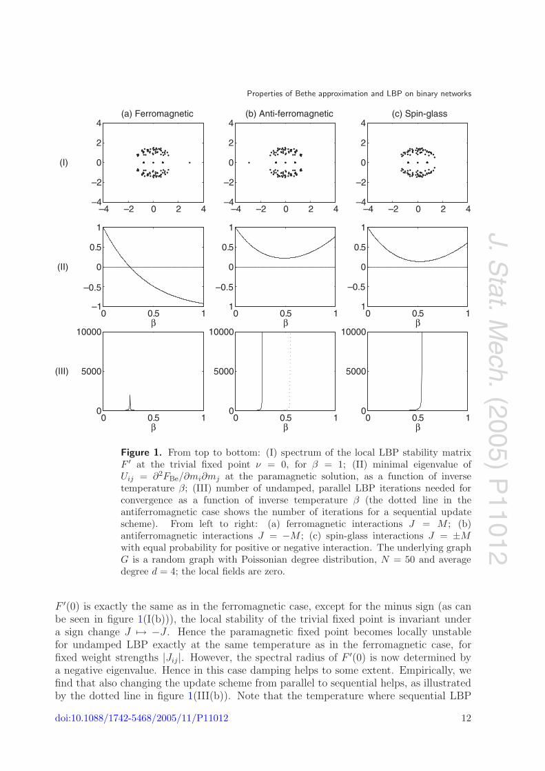
is equal to the matrix B in theorem 1. For high temperature (i.e. small β), theparamagnetic fixed point is locally stable, as is evident from (25). Theorem 1 guaranteesthat this is the only LBP fixed point and that parallel undamped LBP will convergeto it. When we gradually lower the temperature (i.e. increase β), at a sudden pointthe paramagnetic LBP fixed point generally becomes unstable. This seems to hold for allgraphs that have more than one cycle. By a generalization of Perron’s theorem (theorem 3in the appendix), the eigenvalue of the matrix F ′(0) (which has positive entries) with thelargest absolute value is actually positive. This property of the spectrum can be clearlyseen in figure 1(I(a)), where most eigenvalues are distributed in a roughly circular form,except for one outlier on the positive real axis. Thus the onset of instability of theparamagnetic LBP fixed point coincides with this outlier crossing the complex unit circle;the paramagnetic fixed point bifurcates and two new stable fixed points arise, describingthe two ferromagnetic states. Since B = F ′(0), we conclude that the sufficient conditionin theorem 1 for convergence to a unique fixed point is sharp in this case.

At high temperature, the corresponding stationary point of the Bethe free energy is aminimum. However, as illustrated in figure 1(II(a)), at a certain critical temperature theHessian is no longer positive definite. In the appendix, we prove the following theorem:

Theorem 2. For Jij ≥ 0 and θi = 0, the critical temperature at which the paramagneticBethe free energy minimum disappears is equal to the critical temperature at which theparamagnetic LBP fixed point becomes unstable.

Proof. See appendix. �Beyond the transition temperature, LBP converges to either of the two new fixed

points describing the two ferromagnetic phases. As can be seen in figure 1(III(a)), thenumber of LBP iterations needed for convergence has a peak precisely at the criticaltemperature; far from the phase transition, LBP converges rapidly to a stable fixed point.

4.2. Antiferromagnetic interactions

For purely antiferromagnetic interactions, i.e. all Jij < 0, the situation is different. Again,for high temperature, the paramagnetic fixed point is the unique fixed point, is locallystable and has the complete message space as an attractor. Since the local stability matrix

doi:10.1088/1742-5468/2005/11/P11012 11

J.Stat.M

ech.(2005)

P11012

Properties of Bethe approximation and LBP on binary networks

–4

–2

0

2

4(a) Ferromagnetic

–4

–2

0

2

4(b) Anti-ferromagnetic

–4

–2

0

2

4(c) Spin-glass

0 0.5 1–1

0

0.5

1

β0 0.5 1

1

0

0.5

1

β0 0.5 1

1

0

0.5

1

β

0 0.5 1β

0 0.5 1β

0 0.5 1β

–4 –2 0 2 4 –4 –2 0 2 4 –4 –2 0 2 4

–0.5 –0.5

(I)

(II)

(III)

0

5000

10000

0

5000

10000

0

5000

10000

–0.5

Figure 1. From top to bottom: (I) spectrum of the local LBP stability matrixF ′ at the trivial fixed point ν = 0, for β = 1; (II) minimal eigenvalue ofUij = ∂2FBe/∂mi∂mj at the paramagnetic solution, as a function of inversetemperature β; (III) number of undamped, parallel LBP iterations needed forconvergence as a function of inverse temperature β (the dotted line in theantiferromagnetic case shows the number of iterations for a sequential updatescheme). From left to right: (a) ferromagnetic interactions J = M ; (b)antiferromagnetic interactions J = −M ; (c) spin-glass interactions J = ±Mwith equal probability for positive or negative interaction. The underlying graphG is a random graph with Poissonian degree distribution, N = 50 and averagedegree d = 4; the local fields are zero.

F ′(0) is exactly the same as in the ferromagnetic case, except for the minus sign (as canbe seen in figure 1(I(b))), the local stability of the trivial fixed point is invariant undera sign change J → −J . Hence the paramagnetic fixed point becomes locally unstablefor undamped LBP exactly at the same temperature as in the ferromagnetic case, forfixed weight strengths |Jij|. However, the spectral radius of F ′(0) is now determined bya negative eigenvalue. Hence in this case damping helps to some extent. Empirically, wefind that also changing the update scheme from parallel to sequential helps, as illustratedby the dotted line in figure 1(III(b)). Note that the temperature where sequential LBP

doi:10.1088/1742-5468/2005/11/P11012 12

J.Stat.M

ech.(2005)

P11012

Properties of Bethe approximation and LBP on binary networks

stops converging roughly coincides with the minimum of the smallest eigenvalue of U(compare figures 1(II(b)) and 1(III(b))). This observation seems to be generic, i.e. not justa coincidence for the particular instance in figure 1. We have no theoretical explanationfor this at the moment, but it might be possible to get such an explanation by relating Uwith F ′(0), using a technique similar to the one applied in the proof of theorem 2 givenin the appendix.

4.3. Spin-glass interactions

Now consider spin-glass interactions, i.e. all Jij are distributed around 0 such that〈Jij〉 ≈ 0. This case is illustrated in figure 1(c). Here the eigenvalues of the local stabilitymatrix are distributed in a roughly circular form, without an outlier with a large absolutevalue. Note the surprising similarity between the spectra in the different cases; we haveno explanation for this similarity, nor for the roughly circular form of the distribution ofthe majority of the eigenvalues.

Although the paramagnetic Bethe free energy minimum generally does not disappearwhen lowering the temperature, LBP does not converge any longer once the trivial fixedpoint becomes unstable, despite the possible existence of other, stable, fixed points.Neither damping nor changing the update scheme seems to help in this case. Empiricallywe find that the temperature at which the trivial LBP fixed point becomes locally unstableroughly coincides with the temperature at which the lowest eigenvalue of U attains itsminimal value [23]. Again, we have no theoretical explanation for this observation.

5. Estimates of the phase transition temperatures

In this section we estimate the critical temperatures corresponding to the onset ofinstability of the LBP paramagnetic fixed point (which we discussed qualitatively inthe previous section) for a random graph with random interactions. The method isclosely related to the cavity method at the replica-symmetric level (see e.g. [24, 18, 25]).A similar analysis of the stability of the LBP paramagnetic fixed point has been doneby Kabashima [26]; however, the results reported in that work are limited to the case ofinfinite connectivity (i.e. the limit N → ∞, d → ∞). In this case, the results turn out to beidentical to the condition of replica symmetry breaking derived by Almeida and Thouless(the ‘AT line’) [27]. The analysis we present below essentially extends the analysis of [26]to the larger class of arbitrary degree distribution random graphs, which includes Erdos–Renyi graphs (with Poissonian degree distribution, as well as fixed degree random graphs)and power-law graphs (which have power-law degree distributions), amongst others.

5.1. Random graphs with arbitrary degree distributions

We consider arbitrary degree distribution random graphs [28]. This class of random graphshas a prescribed expected degree distribution P (d); apart from that they are completelyrandom. Given an expected degree distribution P (d) and the number of nodes N , aparticular sample of the corresponding ensemble of random graphs can be constructedas follows: for each node i, independently draw an expected degree δi from the degreedistribution P (d); then, for each pair of nodes (i, j), independently connect them withprobability δiδj/

∑i δi; the expected degree of node i is then indeed 〈di〉 = δi. We define

the average degree 〈d〉 :=∑

d P (d)d and the second moment 〈d2〉 :=∑

d P (d)d2.

doi:10.1088/1742-5468/2005/11/P11012 13

J.Stat.M

ech.(2005)

P11012

Properties of Bethe approximation and LBP on binary networks

We consider the case of vanishing local fields (i.e. θi = 0) and draw the weights Jij

independently from some probability distribution P (J). We also assume that the weightsare independent of the graph structure.

5.2. Estimating the PA–FE transition temperature

Assume P (d) to be given and N to be large. Assume that x is an eigenvector witheigenvalue 1 of A := F ′(0), the Jacobian of the parallel LBP update at the paramagneticfixed point ν = 0. Using (17),

xij =∑

kl

Aij,klxkl = tanh(βJij)∑

k∈Ni\j

xki. (26)

Consider an arbitrary spin i; conditional on the degree di of that spin, we can calculatethe expected value of xij as follows:

E (xij | di) = E

tanh(βJij)∑

k∈Ni\j

xki

∣∣∣∣∣∣di

(27a)

= E (tanh(βJij)) E

∑

k∈Ni\j

xki

∣∣∣∣∣∣di

(27b)

= 〈tanh βJ〉 (di − 1)∑

dk

P (dk | di, k ∈ Ni)E (xki | di, dk) (27c)

≈ 〈tanh βJ〉 (di − 1)∑

dk

P (dk | di, k ∈ Ni)E (xki | di) (27d)

using, subsequently: (a) equation (26); (b) the independence of the weights from the graphstructure; (c) conditioning on the degree dk of spin k and the equivalence of the variousk ∈ Ni \ j; and, finally, (d) neglecting the correlation between xki and dk, given di. Wehave no formal argument for the validity of this approximation, but the result accuratelydescribes the outcomes of numerical experiments.

For arbitrary degree distribution random graphs, the probability of dk given the degreedi and the fact that k is a neighbour of i is given by (see [28])

P (dk | di, k ∈ Ni) =dkP (dk)

〈d〉 .

Hence we obtain the relation

E (xij | di) = 〈tanh βJ〉 (di − 1)∑

dk

dkP (dk)

〈d〉 E (xki | dk) . (28)

A self-consistent non-trivial solution of these equations is E (xij | di) ∝ (di − 1), providedthat

1 = 〈tanh βJ〉(〈d2〉〈d〉 − 1

)

, (29)

doi:10.1088/1742-5468/2005/11/P11012 14

J.Stat.M

ech.(2005)

P11012

Properties of Bethe approximation and LBP on binary networks

0J0

JWithout damping

J

With damping

–0.5 0.5 0J0

–0.5 0.5

0.5

0.4

0.3

0.2

0.1

0

0.5

0.4

0.3

0.2

0.1

0

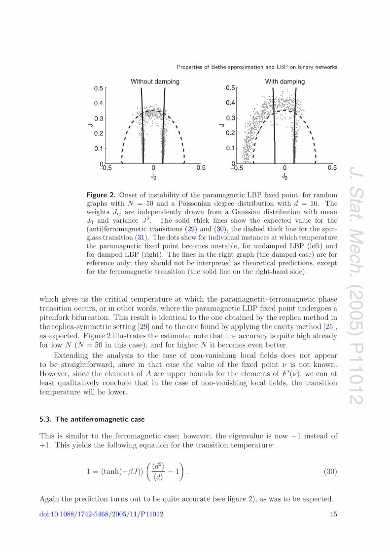
Figure 2. Onset of instability of the paramagnetic LBP fixed point, for randomgraphs with N = 50 and a Poissonian degree distribution with d = 10. Theweights Jij are independently drawn from a Gaussian distribution with meanJ0 and variance J2. The solid thick lines show the expected value for the(anti)ferromagnetic transitions (29) and (30), the dashed thick line for the spin-glass transition (31). The dots show for individual instances at which temperaturethe paramagnetic fixed point becomes unstable, for undamped LBP (left) andfor damped LBP (right). The lines in the right graph (the damped case) are forreference only; they should not be interpreted as theoretical predictions, exceptfor the ferromagnetic transition (the solid line on the right-hand side).

which gives us the critical temperature at which the paramagnetic–ferromagnetic phasetransition occurs, or in other words, where the paramagnetic LBP fixed point undergoes apitchfork bifurcation. This result is identical to the one obtained by the replica method inthe replica-symmetric setting [29] and to the one found by applying the cavity method [25],as expected. Figure 2 illustrates the estimate; note that the accuracy is quite high alreadyfor low N (N = 50 in this case), and for higher N it becomes even better.

Extending the analysis to the case of non-vanishing local fields does not appearto be straightforward, since in that case the value of the fixed point ν is not known.However, since the elements of A are upper bounds for the elements of F ′(ν), we can atleast qualitatively conclude that in the case of non-vanishing local fields, the transitiontemperature will be lower.

5.3. The antiferromagnetic case

This is similar to the ferromagnetic case; however, the eigenvalue is now −1 instead of+1. This yields the following equation for the transition temperature:

1 = 〈tanh(−βJ)〉(〈d2〉〈d〉 − 1

)

. (30)

Again the prediction turns out to be quite accurate (see figure 2), as was to be expected.

doi:10.1088/1742-5468/2005/11/P11012 15

J.Stat.M

ech.(2005)

P11012

Properties of Bethe approximation and LBP on binary networks

5.4. Estimating the PA–SG transition temperature

For the paramagnet–spin-glass phase transition, we can perform a similar calculation, nowassuming that x is an eigenvector with eigenvalue λ on the complex unit circle:

E(|xij |2 | di

)= E

|tanh(βJij)|2∣∣∣∣∣∣

∑

k∈Ni\j

xki

∣∣∣∣∣∣

2∣∣∣∣∣∣di

=⟨tanh2(βJ)

⟩E

∣∣∣∣∣∣

∑

k∈Ni\j

xki

∣∣∣∣∣∣

2∣∣∣∣∣∣di

≈⟨tanh2(βJ)

⟩E

∑

k∈Ni\j

|xki|2∣∣∣∣∣∣di

≈⟨tanh2(βJ)

⟩(di − 1)

∑

dk

P (dk | di, k ∈ Ni)E(|xki|2 | di

),

where, in addition to the assumptions in the PA–FE case, we assumed that the correlationsbetween the various xki can be neglected. Again, we can only motivate this assumptionin that it appears to give correct results.

Using relation (28), we find a non-trivial self-consistent solution E(|xij |2 | di

)∝

(di − 1), if the following equation holds:

1 =⟨tanh2(βJ)

⟩(〈d2〉〈d〉 − 1

)

. (31)

This result is again identical to the one obtained by the cavity method [25], as expected.As illustrated in figure 2 (the dashed line), the accuracy is somewhat less than that of theferromagnetic transition, but is nevertheless quite good, even for N = 50.

For completeness we would like to state that the numerical results reported in [23], inwhich we numerically studied the behaviour of the lowest eigenvalue of U , are accuratelydescribed by the predictions (29) and (31), which supports the hypothesis that thesenotions coincide in the N → ∞ limit.

6. Conclusions

We have derived conditions for the local stability of parallel LBP fixed points, both in theundamped and damped cases for binary networks with pairwise interactions. We haveshown how these relate to the sufficient conditions for uniqueness of the LBP fixed pointand convergence to this fixed point. In particular, we have shown that these sufficientconditions are sharp in the ferromagnetic case, exactly describing the pitchfork bifurcationof the paramagnetic fixed point into two ferromagnetic fixed points. For undamped LBP,the local stability of the paramagnetic fixed point (for vanishing local fields) is invariantunder a sign change of the interactions. For antiferromagnetic interactions, parallelundamped LBP stops converging at the PA–FE transition temperature. Damping or usinga sequential update scheme remedies this defect. However, although the paramagneticminimum of the Bethe free energy does not disappear, the trivial fixed point becomeslocally unstable even for damped LBP at roughly the PA–SG transition temperature.

doi:10.1088/1742-5468/2005/11/P11012 16

J.Stat.M

ech.(2005)

P11012

Properties of Bethe approximation and LBP on binary networks

Finally, for interactions that are dominantly of the spin-glass type, using damping onlymarginally extends the domain of convergence of LBP.

We estimated the PA–FE transition temperature and the PA–SG transitiontemperature for arbitrary degree distribution random graphs. The results are in goodagreement with numerical simulations. How this relates to the AT line is an open questionand beyond the scope of this work.

We believe that the case that we have considered in detail in this work, namelyvanishing local fields θi = 0, is actually the worst-case scenario: numerically it turns outthat adding local fields helps LBP to converge more quickly. We have no proof for thisconjecture at the moment; the local fields make an analytical analysis more difficult andwe have not yet been able to extend the analysis to this more general setting. We leavethe generalization to non-zero local fields as possible future work.

Acknowledgments

The research reported here is part of the Interactive Collaborative Information Systems(ICIS) project, supported by the Dutch Ministry of Economic Affairs, grant BSIK03024.We thank Bastian Wemmenhove and the anonymous reviewer for valuable comments ona draft of this paper.

Appendix: Proof of theorem 2

For a square matrix B, we write B ≥ 0 iff all entries of B are non-negative. σ(B) is theset of all eigenvalues of B, ρ(B) is the spectral radius of B, i.e. ρ(B) := max |σ(B)|. Wewill use the following generalization of Perron’s theorem:

Theorem 3. If B ≥ 0, then the spectral radius ρ(B) ∈ σ(B) and there exists an associatedeigenvector x ≥ 0 such that Bx = ρ(B)x.

Proof. See [30, p 670]. �

Applying this theorem to the matrix B defined in (20), we deduce the existence ofan eigenvector x ≥ 0 with Bx = ρ(B)x. Writing Cij := tanh(β |Jij|) and λ := ρ(B), wederive

xij = λ−1Cij

(∑

k∈Ni

xki − xji

)

= λ−1Cij

∑

k∈Ni

xki − λ−1Cji

∑

k∈Nj

xkj − xij

.

Defining Xi :=∑

k∈Nixki, we obtain, by summing over i ∈ Nj ,

Xj =∑

i∈Nj

λCij

λ2 − CijCjiXi −

∑

i∈Nj

CijCji

λ2 − CijCjiXj ,

doi:10.1088/1742-5468/2005/11/P11012 17

J.Stat.M

ech.(2005)

P11012

Properties of Bethe approximation and LBP on binary networks

i.e. X is an eigenvector with eigenvalue 1 of the matrix

Mijρ(B) tanh(β |Jij|)

ρ(B)2 − tanh2(β |Jij|)− δij

∑

k∈Ni

tanh2(β |Jik|)ρ(B)2 − tanh2(β |Jik|)

. (A.1)

Now, if all Jij are positive, and if ρ(B) = 1, this matrix is exactly I −U , where Uij isdefined in (24). Hence, since in this case B = F ′(0), the critical temperature at which theparamagnetic LBP fixed point becomes unstable coincides with the matrix I − U havingan eigenvalue 1, or in other words U having eigenvalue 0. Thus the onset of instability ofthe paramagnetic LBP fixed point in this case exactly coincides with the disappearanceof the paramagnetic Bethe free energy minimum.

References

[1] Bethe H, 1935 Proc. R. Soc. A 150 552[2] Peierls R E, 1936 Proc. Camb. Phil. Soc. 32 477[3] Kikuchi R, 1951 Phys. Rev. 81 988[4] Pelizzola A, 2005 J. Phys. A: Math. Gen. 38 R309[5] Tanaka K, 2002 J. Phys. A: Math. Gen. 35 R81[6] Pearl J, 1988 Probabilistic Reasoning in Intelligent Systems: Networks of Plausible Inference

(San Francisco, CA: Morgan Kaufmann)[7] McEliece R J, MacKay D J C and Cheng J F, 1998 IEEE J. Sel. Areas Commun. 16 140[8] Nishimori H, 2001 Statistical Physics of Spin Glasses and Information Processing—an Introduction

(Oxford: Oxford Press)[9] Yedidia J S, Freeman W T and Weiss Y, 2001 (NIPS*2000): Advances in Neural Information Processing

Systems vol 13, ed L K Saul, Y Weiss and L Bottou (Cambridge, MA: MIT Press) pp 689–95[10] Braunstein A and Zecchina R, 2004 J. Stat. Mech. P06007[11] Freeman W, Pasztor E and Carmichael O, 2000 Int. J. Comput. Vis. 40 25[12] Kappen H, 2002 Modelling Biomedical Signals (Singapore: World Scientific) pp 3–27[13] Baxter R, 1982 Exactly Solved Models in Statistical Mechanics (New York: Academic)[14] Welling M and Teh Y W, 2003 Artif. Intell. 143 19[15] Kschischang F R, Frey B J and Loeliger H-A, 2001 IEEE Trans. Inf. Theory 47 498[16] Heskes T, Albers C and Kappen H J, 2003 (UAI-03): Proc. 19th Annual Conf. on Uncertainty in Artificial

Intelligence (San Francisco, CA: Morgan Kaufmann) pp 313–20[17] Heskes T, 2004 Neural Comput. 16 2379[18] Mezard M and Parisi G, 2001 Eur. Phys. J. B 20 217[19] Kuznetsov Y A, 1988 Elements of Applied Bifurcation Theory (Applied Mathematical Sciences vol 112)

2nd edn (New York: Springer)[20] Mooij J and Kappen H, 2005 (UAI-05): Proc. 21st Annual Conf. on Uncertainty in Artificial Intelligence

(Corvallis, OR: AUAI Press) pp 396–403[21] Ihler A T, Fisher J W and Willsky A S, 2005 J. Mach. Learning Res. 6 905[22] Welling M and Teh Y W, 2001 (UAI-01): Proc. 17th Annual Conf. on Uncertainty in Artificial Intelligence

(San Francisco, CA: Morgan Kaufmann) pp 554–61[23] Mooij J and Kappen H, 2005 (NIPS*2004): Advances in Neural Information Processing Systems vol 17,

ed L K Saul, Y Weiss and L Bottou (Cambridge, MA: MIT Press)[24] Mezard M, Parisi G and Virasoro M A, 1987 Spin Glass Theory and Beyond (Singapore: World Scientific)[25] Wemmenhove B, Nikoletopoulos T and Hatchett J P L, 2004 Preprint cond-mat/0405563[26] Kabashima Y, 2003 J. Phys. Soc. Japan 72 1645[27] de Almeida J R L and Thouless D J, 1978 J. Phys. A: Math. Gen. 11 983[28] Newman M E J, Strogatz S H and Watts D J, 2001 Phys. Rev. E 64 026118[29] Leone M, Vazquez A, Vespignani A and Zecchina R, 2002 Eur. Phys. J. B 28 191[30] Meyer C D, 2000 Matrix Analysis and Applied Linear Algebra (Philadelphia, PA: SIAM)

doi:10.1088/1742-5468/2005/11/P11012 18