Embed Size (px)
Citation preview

Nonlinear Analysis: Modelling and Control, 2014, Vol. 19, No. 2, 225–240 225
On the stability of explicit finite difference schemesfor a pseudoparabolic equation with nonlocal conditions
Justina Jachimavicienea, Mifodijus Sapagovasb, Arturas Štikonasb,c,Olga Štikonieneb,c
aVytautas Magnus UniversityVileikos str. 8, LT-44404 Kaunas, [email protected] of Mathematics and Informatics, Vilnius UniversityAkademijos str. 4, LT-08663 Vilnius, [email protected] of Mathematics and Informatics, Vilnius UniversityNaugarduko str. 24, LT-03225 Vilnius, [email protected]; [email protected]
Received: 20 February 2013 / Revised: 6 February 2014 / Published online: 19 February 2014
Abstract. A new explicit conditionally consistent finite difference scheme for one-dimensionalthird-order linear pseudoparabolic equation with nonlocal conditions is constructed. The stabilityof the finite difference scheme is investigated by analysing a nonlinear eigenvalue problem. Thestability conditions are stated and stability regions are described. Some numerical experiments arepresented in order to validate theoretical results.
Keywords: pseudoparabolic equation, nonlocal conditions, explicit finite difference scheme,stability, stability regions, nonlinear eigenvalue problem, three-layer finite difference scheme.
1 Introduction
We consider third-order linear pseudoparabolic equation with nonlocal integral conditions
ut = ηutxx + uxx + f(x, t), x ∈ (0, X), 0 < t 6 T, (1)
u(0, t) = γ0
X∫0
u(x, t) dx+ vl(t), 0 6 t 6 T, (2)
u(X, t) = γ1
X∫0
u(x, t) dx+ vr(t), 0 6 t 6 T, (3)
u(x, 0) = v0(x), x ∈ [0, X], (4)
where η > 0. The goal of this paper is to present explicit finite difference schemes (FDS)for this problem and to investigate their stability properties.
c© Vilnius University, 2014

226 J. Jachimaviciene et al.
In the field of numerical analysis of differential equations, great attention has beendedicated to the development of efficient and accurate methods, mostly of implicit type.Implicit finite difference schemes for linear or nonlinear pseudoparabolic equation withDirichlet boundary conditions were introduced in early 1970s [1, 2]. Stability and con-vergence of finite difference method were investigated in these papers. There are severalsituations in which the use of implicit methods causes a huge amount of computation(for example, systems of very large dimension, in presence of strong nonlinearity). Ex-plicit methods for partial differential equations overcome these difficulties successfully.The main disadvantage of explicit methods concerns their stability. So, the benefits andstability properties of explicit methods have to be deeply analysed for safe exploiting.
Theoretical research of pseudoparabolic equations with nonlocal boundary conditions(NBC) was started due to their applications for complex problems in science and technol-ogy. One of the first results for the third-order pseudoparabolic equations with NBCs wasgiven in monograph [3] for problems of soil dampness dynamics. A number of papersdevoted to underground water flow dynamics modelling by pseudoparabolic equation withNBCs were published later, see [4, 5].
Numerical methods for pseudoparabolic equations with NBCs are of permanent in-terest for researchers during the last decades. The Rothe time-discretization method fora nonlinear pseudoparabolic equation with integral conditions was considered in [6].A numerical method for solving a one-dimensional nonlinear pseudoparabolic equationwith one integral condition in reproducing kernel space was proceeded in [7]. ImplicitFDS for a linear one- and two-dimensional pseudoparabolic equation with various integralconditions are analysed in [8–11].
Applications of pseudoparabolic problems with different boundary conditions includ-ing NBCs are discussed in papers [6, 7] and monograph [12]. Both explicit and implicitFDS for numerical solution of (1) are investigated completely enough for case of parabolicequation (η = 0). Problems with classical boundary conditions are studied in manymonographs (for example, [13]). Note that, in the case η 6= 0, third-order derivative utxxdoes not allow to write two-layer explicit FDS for (1).
Three-layer FDS for the second order parabolic equation (equation (1) in the caseη = 0) with classical boundary conditions are investigated in details in [13]. Such schemesfor problems with NBCs are studied in [14, 15]. Following [14], we can convert three-layer FDS to two-layer system
Wj+1 = SWj + F,
where Wj ,F are vectors and matrix S is non-symmetrical due to nonlocal conditions.Energy norm of vector Wj is connected with the eigenvalue problem for finite differ-ence operator with NBCs. Nonlinear eigenvalue problem is also used for investigation ofspectrum of matrix S. A number of papers devoted to the investigation of spectrum ofdifferential or difference operators with NBCs and their applications. We refer to [16–26]for detailed discussions.
Applying the methodology of [14] to investigation of three-layer schemes with non-local conditions, we prove that stable explicit FDS can be constructed using specificapproximation of third-order derivative.
www.mii.lt/NA

Stability of explicit FDS for a pseudoparabolic equation with nonlocal conditions 227
The rest of this paper is organised as follows. We formulate a difference problem forapproximation of the pseudoparabolic problem (1)–(4) in Section 2. Stability regions andstability conditions are investigated in Section 3. Results of numerical experiments arepresented in Section 4. Final conclusions are done in Section 5.
2 Finite difference scheme
2.1 Three-layer explicit scheme
Let us write three-layer explicit FDS for differential problem (1)–(4). To this aim, we usespecific approximation of the third-order derivative. As far as the authors are aware, suchapproximation firstly was used for solution of pseudoparabolic equation in [27, 28].
We introduce grids with uniform steps
ωh := {xi: xi = hi, i = 0,M}, h =X
M,
ωτ := {tj : tj = τj, j = 0, N}, τ =T
N,
ωh := {x1, x2, . . . , xM−1}, ωτ := {t1, t2, . . . , tN−1}. In the domain [0, X]× [0, T ], weuse grids ω := ωh × ωτ , ω := ωh × ωτ .
We use the notation U ji := U(xi, tj) for functions defined on the grid (or parts of thisgrid) ωh × ωτ . Let us define vectors U = (U0, U1, . . . , UM )> and U = (U1, U2, . . . ,UM−1)>.
If solution u of differential problem (1)–(4) is smooth enough, then the followingapproximation can be written in any point (xi, tj) ∈ ω:
(utxx)ji = (uxxt)ji =
1
h2((ut)
ji−1 − 2(ut)
ji + (ut)
ji+1
)+O(h2).
In order to construct explicit FDS, we approximate (ut)ji by the forward differences, and
another two derivatives by the backward differences:
(utxx)ji =1
h2
(uji−1 − u
j−1i−1
τ− 2
uj+1i − ujiτ
+uji+1 − u
j−1i+1
τ+O(τ)
)+O(h2)
=1
τ
(uji−1 − 2uj+1i + uji+1
h2−uj−1i−1 − 2uji + uj−1i+1
h2
)+O
(τ
h2+ h2
). (5)
Let us consider three-layer FDS for problem (1)–(4)
U j+1i − U j−1i
2τ=η
τ
(U ji−1 − 2U j+1
i + U ji+1
h2−U j−1i−1 − 2U ji + U j−1i+1
h2
)+U ji−1 − (U j+1
i + U j−1i ) + U ji+1
h2+ F ji , (xi, tj) ∈ ω, (6)
Nonlinear Anal. Model. Control, 2014, Vol. 19, No. 2, 225–240
228 J. Jachimaviciene et al.
U j0 = γ0L(Uj) + V jl , tj ∈ ωτ , (7)
U jM = γ1L(Uj) + V jr , tj ∈ ωτ , (8)
U0i = (V0)i, xi ∈ ωh, (9)
U1i = (V1)i, xi ∈ ωh, (10)
where L(Uj) = (U j0 + U jM )h/2 +
∑M−1i=1 U ji h. In order to use three-layer scheme, we
need to impose an additional condition on the first layer. One way of proceeding it is toapply at the first step the two-layer implicit scheme of accuracy O(τ2 + h2) [13].
We could rewrite equation (6) as
U j+1i − U ji
2τ=η
τ
(U ji−1 − 2U ji + U ji+1
h2− 2U j+1
i − 2U jih2
−U j−1i−1 − 2U j−1i + U j−1i+1
h2+
2U ji − 2U j−1i
h2
)+U ji−1 − 2U ji + U ji+1
h2+
2U ji − (U j−1i + U j+1i )
h2+ F ji . (11)
Taking into account (5), we get that difference problem (6)–(10) approximates differentialproblem (1)–(4) conditionally with truncation error O(τ2 + h2 + τ/h2) as τ = o(h2).
If η = 0, equation (6) corresponds to Dufort–Frankel scheme, which is conditionallyconsistent with error O(τ2 + h2 + τ2/h2) to the second order parabolic problem withDirichlet boundary conditions, and it is unconditionally stable.
2.2 Two-layer system and nonlinear eigenvalue problem
According to methodology of [14], we reduce the three-layer FDS (6)–(10) to two-layersystem. Firstly, we consider (7) and (8) as a linear system with unknowns U j0 and U jMand write modified NBCs
U j0 = γ0L(Uj)
+ V jl , U jM = γ1L(Uj)
+ V jr , (12)
where γ0 = γ0/d, γ1 = γ1/d, L(Uj) =∑M−1i=1 U ji h, d = 1− h(γ0 + γ1)/2 and
V jl =V jl + hcj
d, V jr =
V jr − hcj
d, cj =
γ0Vjr − γ1V
jl
2.
Note that d > 0 for γ0 + γ1 6 0 and d > 0 if h is sufficiently small (h < 2/(γ0 + γ1))in the case γ0 + γ1 > 0.
Substituting expressions (12) in equation (11), we rewrite FDS (6)–(8) for every j =1, N − 1 as
AUj+1 + BUj + CUj−1 = 2τFj , (13)
www.mii.lt/NA

Stability of explicit FDS for a pseudoparabolic equation with nonlocal conditions 229
where A, B, C are (M − 1)× (M − 1) matrices:
A =(1 + 2(τ + 2η)h−2
)I, B = 2(τ + η)Λ− 4(τ + 2η)h−2I,
C =(−1 + 2(τ + 2η)h−2
)I− 2ηΛ,
Λ =1
h2
2− γ0h −1− γ0h −γ0h . . . −γ0h −γ0h−1 2 −1 . . . 0 00 −1 2 . . . 0 0· · · · · · · · · · · · · · · · · ·0 0 0 . . . 2 −1−γ1h −γ1h −γ1h . . . −1− γ1h 2− γ1h
,
and I be the identity (M − 1) × (M − 1) matrix, Fj be column vectors ((M − 1) × 1matrices).
Eigenvalue problemΛU = λU
is equivalent to the eigenvalue problem for the difference operator with NBCs (see [14]for detailed explanation)
−Ui−1 − 2Ui + Ui+1
h2= λUi, xi ∈ ωh, (14)
U0 = γ0L(U), UM = γ1L(U). (15)
Let us introduce 2(M − 1)-order vector
Wj =
(Uj
Uj−1
), j = 1,M.
Then three-layer FDS (13) can be written as two-layer scheme [13, 14]
Wj+1 = SWj + 2τGj , j = 1,M − 1, (16)
where
S =
(−A−1B −A−1C
I 0
), Gj =
(A−1Fj
0
),
and 0 is zero matrix (or vector). Matrix S is nonsymmetric except case γ0 = γ1 = 0 (aswell as matrices Λ, B and C).
In the next section, stability of FDS (16) will be analysed using spectrum of matrix S.So, we investigate eigenvalues of this matrix which are determined as the roots of thefollowing equation:
det(S− µI) = 0 or det
(−A−1B− µI −A−1C
I −µI
)= 0.
It follows thatdet(µ2I + µA−1B + A−1C
)= 0
Nonlinear Anal. Model. Control, 2014, Vol. 19, No. 2, 225–240
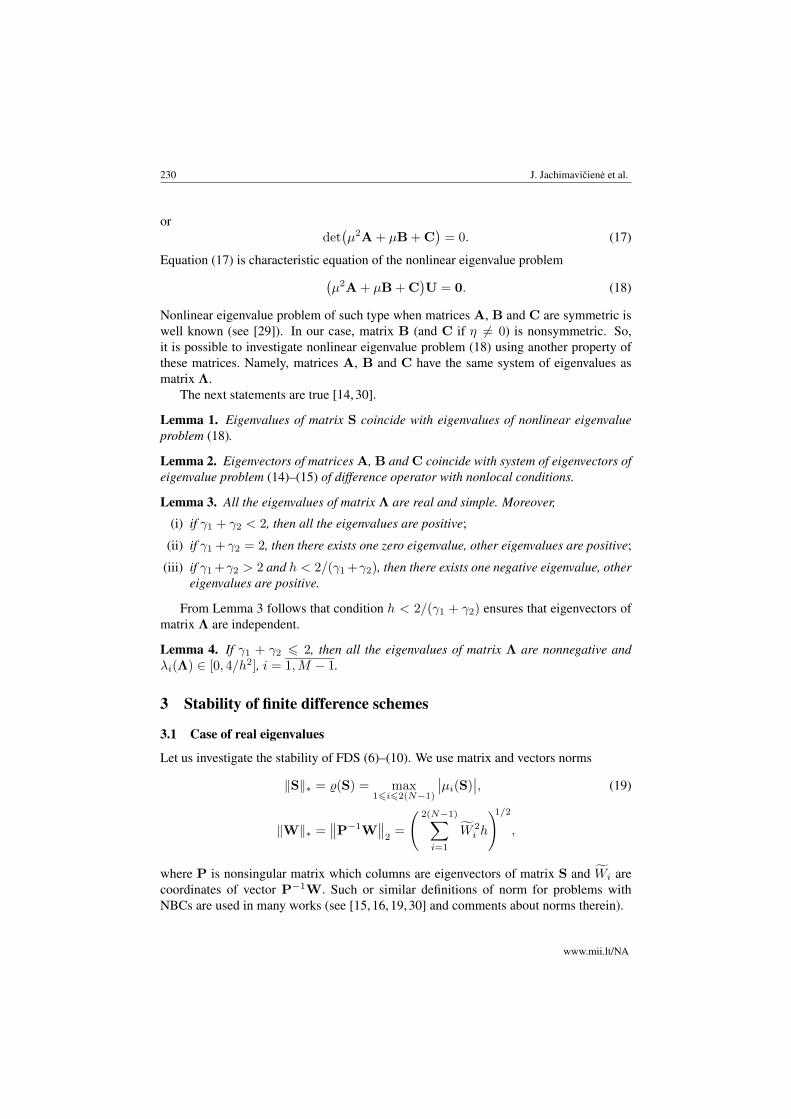
230 J. Jachimaviciene et al.
ordet(µ2A + µB + C
)= 0. (17)
Equation (17) is characteristic equation of the nonlinear eigenvalue problem(µ2A + µB + C
)U = 0. (18)
Nonlinear eigenvalue problem of such type when matrices A, B and C are symmetric iswell known (see [29]). In our case, matrix B (and C if η 6= 0) is nonsymmetric. So,it is possible to investigate nonlinear eigenvalue problem (18) using another property ofthese matrices. Namely, matrices A, B and C have the same system of eigenvalues asmatrix Λ.
The next statements are true [14, 30].
Lemma 1. Eigenvalues of matrix S coincide with eigenvalues of nonlinear eigenvalueproblem (18).
Lemma 2. Eigenvectors of matrices A, B and C coincide with system of eigenvectors ofeigenvalue problem (14)–(15) of difference operator with nonlocal conditions.
Lemma 3. All the eigenvalues of matrix Λ are real and simple. Moreover,
(i) if γ1 + γ2 < 2, then all the eigenvalues are positive;
(ii) if γ1 + γ2 = 2, then there exists one zero eigenvalue, other eigenvalues are positive;
(iii) if γ1 +γ2 > 2 and h < 2/(γ1 +γ2), then there exists one negative eigenvalue, othereigenvalues are positive.
From Lemma 3 follows that condition h < 2/(γ1 + γ2) ensures that eigenvectors ofmatrix Λ are independent.
Lemma 4. If γ1 + γ2 6 2, then all the eigenvalues of matrix Λ are nonnegative andλi(Λ) ∈ [0, 4/h2], i = 1,M − 1.
3 Stability of finite difference schemes
3.1 Case of real eigenvalues
Let us investigate the stability of FDS (6)–(10). We use matrix and vectors norms
‖S‖∗ = %(S) = max16i62(N−1)
∣∣µi(S)∣∣, (19)
‖W‖∗ =∥∥P−1W∥∥
2=
(2(N−1)∑i=1
W 2i h
)1/2,
where P is nonsingular matrix which columns are eigenvectors of matrix S and Wi arecoordinates of vector P−1W. Such or similar definitions of norm for problems withNBCs are used in many works (see [15, 16, 19, 30] and comments about norms therein).
www.mii.lt/NA

Stability of explicit FDS for a pseudoparabolic equation with nonlocal conditions 231
According to definition of matrix S norm (19), stability condition for FDS (16) canbe written as
%(S) 6 1.
Theorem 1. If condition γ1 + γ2 6 2 is true, then %(S) 6 1 and FDS is stable.
Proof. Eigenvalues of matrix S can be found from equation (18). Let us denote any eigen-value of Λ as λ and correspondent eigenvector as U. We denote eigenvalues of A, B andC as λ(A), λ(B) and λ(C), respectively. Then we have
λ(A) = 1 +2
h2(τ + 2η),
λ(B) = 2(τ + η)λ− 4
h2(τ + 2η),
λ(C) = −1 +2
h2(τ + 2η)− 2ηλ.
Substituting U into (18), we get quadratic equation
(1 + δ)µ2 + 2((τ + η)λ− δ
)µ+ δ − 1− 2ηλ = 0, (20)
where
δ := β
(τ
2+ η
)> 0, β :=
4
h2> 0.
We rewrite this quadratic equation as
µ2 + bµ+ c = 0 (21)
with coefficients
b :=2(τ + η)λ− 2δ
1 + δ=
2τλ
1 + δ− c− 1, c :=
δ − 1− 2ηλ
1 + δ. (22)
According to Hurwitz criterion, roots of (21) with real coefficients |µ| 6 1 if and only if
c 6 1, |b| 6 c+ 1.
The first inequality of Hurwitz criterion for coefficients (22) gives condition for λ
δ − 1− 2ηλ 6 1 + δ ⇐⇒ ηλ > −1. (23)
The second inequality is equivalent to
2ηλ− 2δ 6 2(τ + η)λ− 2δ 6 2δ − 2ηλ
or0 6 λ 6
2δ
τ + 2η= β. (24)
Condition τλ > 0 is stronger than (23). Lemma 4 implies that λ ∈ [0, β] when γ0+γ1 6 2and the theorem is proved.
Nonlinear Anal. Model. Control, 2014, Vol. 19, No. 2, 225–240
232 J. Jachimaviciene et al.
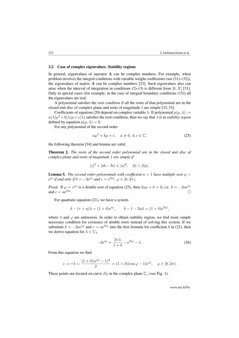
3.2 Case of complex eigenvalues. Stability regions
In general, eigenvalues of operator Λ can be complex numbers. For example, whenproblem involves the integral conditions with variable weight coefficients (see (31)–(32)),the eigenvalues of matrix Λ can be complex numbers [23]. Such eigenvalues also canarise when the interval of integration in conditions (2)–(3) is different from [0, X] [31].Only in special cases (for example, in the case of integral boundary conditions (15)) allthe eigenvalues are real.
A polynomial satisfies the root condition if all the roots of that polynomial are in theclosed unit disc of complex plane and roots of magnitude 1 are simple [32, 33].
Coefficients of equation (20) depend on complex variable λ. If polynomial p(µ, λ) :=a(λ)µ2 +b(λ)µ+c(λ) satisfies the root condition, then we say that λ is in stability regiondefined by equation p(µ, λ) = 0.
For any polynomial of the second order
aµ2 + bµ+ c, a 6= 0, b, c ∈ C, (25)
the following theorem [34] and lemma are valid.
Theorem 2. The roots of the second order polynomial are in the closed unit disc ofcomplex plane and roots of magnitude 1 are simple if
|c|2 + |ab− bc| 6 |a|2, |b| < 2|a|.
Lemma 5. The second order polynomials with coefficient a = 1 have multiple root µ =eiϕ if and only if b = −2eiϕ and c = e2iϕ, ϕ ∈ [0, 2π).
Proof. If µ = eiϕ is a double root of equation (25), then 2aµ + b = 0, i.e. b = −2aeiϕ
and c = ae2iϕ.
For quadratic equation (21), we have a system
δ − (τ + η)λ = (1 + δ)eiϕ, δ − 1− 2ηλ = (1 + δ)e2iϕ,
where λ and ϕ are unknowns. In order to obtain stability region, we find more simplenecessary condition for existence of double roots instead of solving this system. If wesubstitute b = −2aeiϕ and c = ae2iϕ into the first formula for coefficient b in (22), thenwe derive equation for λ ∈ Cλ
−2eiϕ =2τλ
1 + δ− e2iϕ − 1. (26)
From this equation we find
z := τλ =(1 + δ)(eiϕ − 1)2
2= (1 + δ)(cosϕ− 1)eiϕ, ϕ ∈ [0, 2π).
These points are located on curve Dδ in the complex plane Cz (see Fig. 1).
www.mii.lt/NA

Stability of explicit FDS for a pseudoparabolic equation with nonlocal conditions 233
Fig. 1. Curves Dδ for δ = 0,0.5, 1, 3.
(a) complex plane Cz , z = τλ (b) complex plane CλFig. 2. Stability regions for Dufort–Frankel scheme (η = 0) in thecase δ = α = τβ/2 = 2τ/h2.
Remark 1. Curve Dδ gives necessary condition for double root. For z = 0 ∈ Dδ , wehave simple roots µ1 = 1 and µ2 = (δ − 1)/(δ + 1).
If η = 0, then we have Dufort–Frankel scheme for parabolic equation and δ = βτ/2.We introduce new parameter α := 2τ/h2 > 0. Then δ = α for this scheme. Fromequality
(1 + α)µ2 + 2(z − α)µ+ α− 1 = 0, z = τλ,
we express z = α − (µ − µ−1)/2 − α(µ + µ−1)/2. Substituting µ = eiϕ, ϕ ∈ [0, 2π),into this expression, we get formula for boundary of the stability region
z = α(1− cosϕ)− i sinϕ.
The boundary is ellipse (x− α)2/α2 + y2 = 1, z = x+ iy (see Fig. 2(a)). If α = 0, theellipse degenerates into a segment [−i,+i] of the imaginary axis and we have double rootsin the points ±i (see Fig. 1, the case δ = 0). We can easily get the regions in complexplane Cλ using homothety (centre is z = 0 and ratio is equal to 1/τ , see Fig. 2(b)). Inthe complex plane Cλ, ellipse intersects real axis at points λ = 0 and λ = 4/h2, and thevertical semi-axis is 1/τ .
Now we consider equation (20) in the form (τ > 0)
(1 + δ)µ2 + 2((1 + ξ)z − δ
)µ+ δ − 1− 2ξz = 0, (27)
where ξ := η/τ . Then δ = α(1 + 2ξ).For α = 1, equation (27) has two roots
µ1 = z − 1, µ2 =ξ
1 + ξ
and |µ2| < 1. So, stability region is |z−1| 6 1 for all ξ > 0. The boundary of this regionis S1(1), where Sr(z0) denotes a circle with radius r and centre z0.
The stability regions for α > 1 are presented in Fig. 4. The boundary transforms fromellipse (the case ξ = 0) to circle Sα(α) (the case ξ =∞).
Nonlinear Anal. Model. Control, 2014, Vol. 19, No. 2, 225–240
234 J. Jachimaviciene et al.
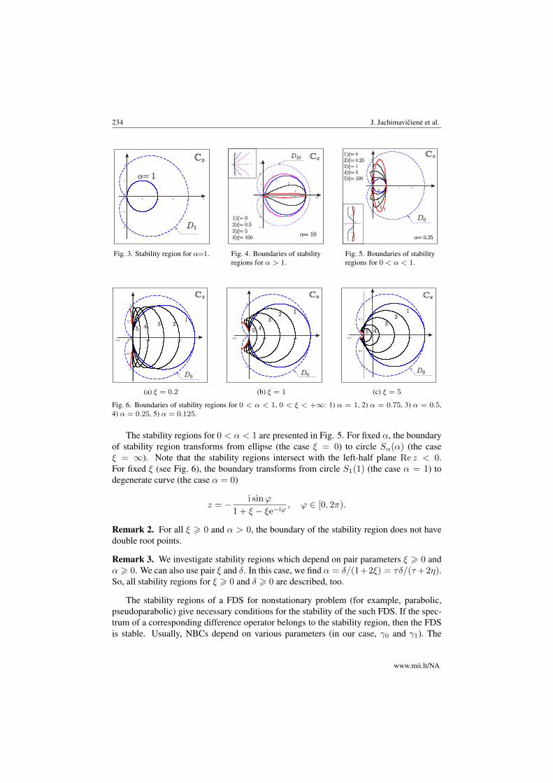
Fig. 3. Stability region for α=1. Fig. 4. Boundaries of stabilityregions for α > 1.
Fig. 5. Boundaries of stabilityregions for 0 < α < 1.
(a) ξ = 0.2 (b) ξ = 1 (c) ξ = 5
Fig. 6. Boundaries of stability regions for 0 < α < 1, 0 < ξ < +∞: 1) α = 1, 2) α = 0.75, 3) α = 0.5,4) α = 0.25, 5) α = 0.125.
The stability regions for 0 < α < 1 are presented in Fig. 5. For fixed α, the boundaryof stability region transforms from ellipse (the case ξ = 0) to circle Sα(α) (the caseξ = ∞). Note that the stability regions intersect with the left-half plane Re z < 0.For fixed ξ (see Fig. 6), the boundary transforms from circle S1(1) (the case α = 1) todegenerate curve (the case α = 0)
z = − i sinϕ
1 + ξ − ξe−iϕ, ϕ ∈ [0, 2π).
Remark 2. For all ξ > 0 and α > 0, the boundary of the stability region does not havedouble root points.
Remark 3. We investigate stability regions which depend on pair parameters ξ > 0 andα > 0. We can also use pair ξ and δ. In this case, we find α = δ/(1+2ξ) = τδ/(τ +2η).So, all stability regions for ξ > 0 and δ > 0 are described, too.
The stability regions of a FDS for nonstationary problem (for example, parabolic,pseudoparabolic) give necessary conditions for the stability of the such FDS. If the spec-trum of a corresponding difference operator belongs to the stability region, then the FDSis stable. Usually, NBCs depend on various parameters (in our case, γ0 and γ1). The
www.mii.lt/NA
Stability of explicit FDS for a pseudoparabolic equation with nonlocal conditions 235
spectrum of the operator Λ must lie in stability region of the investigated FDS. In generalcase, points of the spectrum move in the complex plane when values of the parametersin the NBCs vary. These points can be complex (problems with NBCs often are not self-adjoint). The spectrum of the operator Λ with various integral boundary conditions isinvestigated in [31]. If we compare results about the spectrum of the operator Λ with thestability regions for the investigated FDS, then we can find parameters (and domains ofthem), such that FDS is stable.
For example, in the case of NBCs (8)–(9), the spectrum of the operator Λ belongs to[0, 4/h2] when γ0 + γ1 6 2. On the other hand, [0, 4/h2] belongs to stability region forall values of parameters (for all ξ > 0 and α > 0, the boundary of the stability regionintersects real axis at points λ = 0 and λ = 4/h2). So, the stability of FDS follows.
4 Numerical experiment
We now present some numerical results demonstrating the efficiency of conditionallyconsistent explicit scheme. Also, we investigated the dependence of error on parameter ηand time interval T . We consider a model problem (1)–(4) in the case X = 1. The right-hand side function f , initial and boundary conditions were prescribed to satisfy the givenexact solution
u∗(x, t) = x(x− 1) sin t.
We consider uniform grids with different mesh sizes h and τ and analyse the con-vergence and accuracy of the computed solution from the present scheme. Differenceproblem (6)–(10) approximates differential problem (1)–(4) conditionally with truncationerror
O(τ
h2+ τ2 + h2
).
To demonstrate the accuracy of FDS (6)–(9), we calculate the maximum norm of the errorof the numerical solution as
ε = maxi=0,...,M
∣∣UNi − u∗(xi, tN )∣∣.
The results of the numerical test are listed for γ0 = γ1 = −10.The dependence of ε versus grid step sizes τ, h and their quotient τ/h2 is presented
in Tables 1–3.
Table 1. The errors for different h, τ (γ0 = γ1 = −10,η = 1, T = 10).
h τ τ/h2 ε0.5 4.096 · 10−2 0.164 2.23581 · 10−2
0.25 5.120 · 10−3 0.082 5.95492 · 10−3
0.125 6.400 · 10−4 0.041 1.59542 · 10−3
0.0625 8.000 · 10−5 0.020 4.47834 · 10−4
0.03125 1.000 · 10−5 0.010 1.35981 · 10−4
0.015625 1.250 · 10−6 0.005 4.59697 · 10−5
Nonlinear Anal. Model. Control, 2014, Vol. 19, No. 2, 225–240

236 J. Jachimaviciene et al.
Table 2. The errors for different h, τ = h4 (γ0 = γ1 =−10, η = 1, T = 2).
h τ = h4 τ/h2 ε0.5 0.06250 0.250 3.7921 · 10−2
0.25 0.00391 0.063 9.5027 · 10−3
0.125 0.00024 0.016 2.3762 · 10−3
0.0625 0.00002 0.004 5.9405 · 10−4
0.03125 9.53674 · 10−7 0.001 1.48514 · 10−4
0.015625 5.96046 · 10−8 0.00025 3.71135 · 10−5
Table 3. The errors for different h, τ (γ0 = γ1 = −10,η = 1, T = 2).
h τ = h2 τ/h2 ε1/2 0.25000 1.0 4.83638 · 10−2
1/22 0.06250 1.0 2.49875 · 10−2
1/23 0.01563 1.0 1.93727 · 10−2
1/24 0.00391 1.0 2.13888 · 10−2
· · · · · · · · · · · ·1/28 1.52588 · 10−5 1.0 2.20605 · 10−2
1/29 3.81470 · 10−6 1.0 2.20625 · 10−2
1/210 9.53674 · 10−7 1.0 2.20629 · 10−2
Table 4. The errors for different T : (a) h = 0.05, τ =0.0003125, η = 1, γ0 = γ1 = −10; (b) h = 0.03125,τ = 10−5, η = 1, γ0 = −10, γ1 = 1.
(a) (b)
T ε1.57 1.98300 · 10−3
6.28 1.91139 · 10−3
9.42 1.91789 · 10−3
12.60 1.91998 · 10−3
T ε1 7.64456 · 10−4
2 2.21989 · 10−3
5 4.50859 · 10−2
Numerical experiment illustrates the dependence of error on the quotient τ/h2. Wesee that the numerical errors decays as the mesh size decrease. If we reduce h twice andτ eight times, then τ/h2 reduces twice. Hence, the error of the solution also reduces, butit is difficult to evaluate how fast it reduces (see Table 1). However, this is possible forspecial values τ and h. If τ = h4, then truncation error is O(τ/h2 + τ2 + h2) = O(h2).Therefore, the error of the solution reduces 4 times as h reduces twice. These results areconfirmed by simulation presented in Table 2. Similarly, for τ = h2, truncation error isO(1), thus the error stays roughly constant as h and τ are reduced (Table 3).
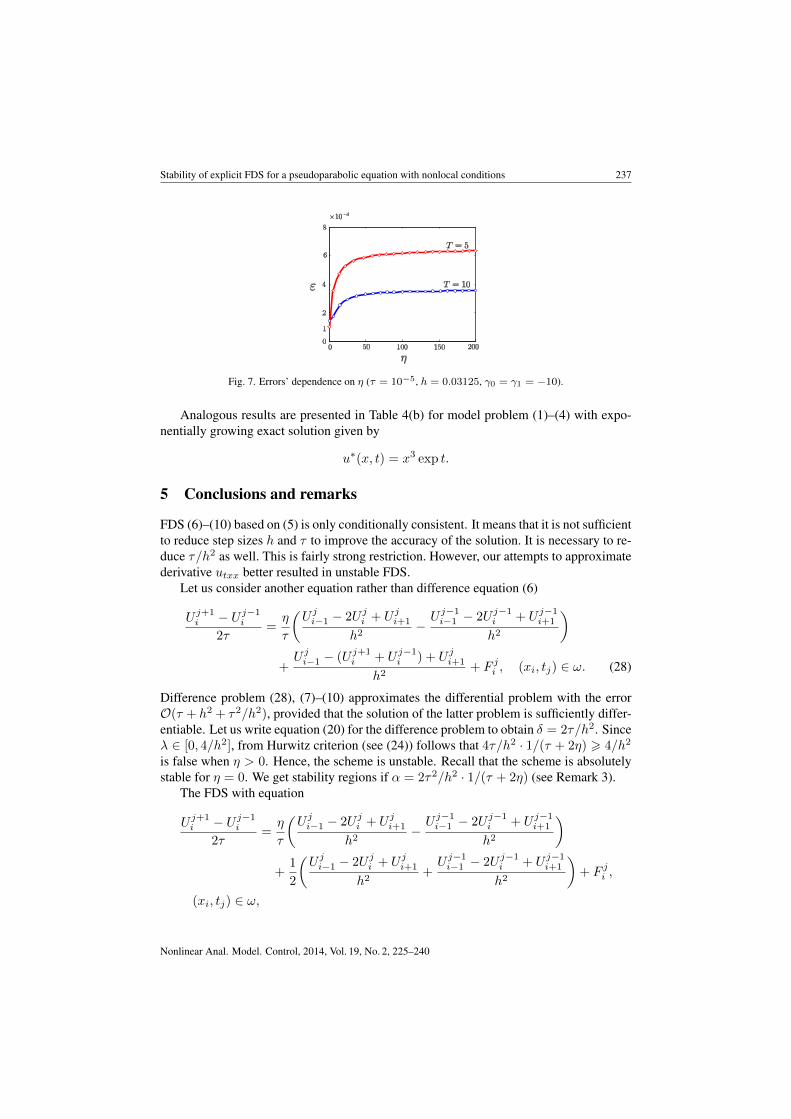
In Fig. 7 we sketch dependence of the absolute maximum errors on η for two differenttime intervals (T = 5 and T = 10). The error grows linearly for small η but saturates forlarge η and approaches some constant value.
Some of the FDS for the second order parabolic equations with nonlocal integralconditions have the following property [35, 36]. Calculations show that the scheme isstable when T = 1, but the error becomes unbounded as T increases. Thus, FDS is notuniformly stable with respect to t. Results in Table 4(a) are important because the error ofthe numerical solution obtained using FDS (6)–(9) do not grow with the interval of time.
www.mii.lt/NA
Stability of explicit FDS for a pseudoparabolic equation with nonlocal conditions 237
Fig. 7. Errors’ dependence on η (τ = 10−5, h = 0.03125, γ0 = γ1 = −10).
Analogous results are presented in Table 4(b) for model problem (1)–(4) with expo-nentially growing exact solution given by
u∗(x, t) = x3 exp t.
5 Conclusions and remarks
FDS (6)–(10) based on (5) is only conditionally consistent. It means that it is not sufficientto reduce step sizes h and τ to improve the accuracy of the solution. It is necessary to re-duce τ/h2 as well. This is fairly strong restriction. However, our attempts to approximatederivative utxx better resulted in unstable FDS.
Let us consider another equation rather than difference equation (6)
U j+1i − U j−1i
2τ=η
τ
(U ji−1 − 2U ji + U ji+1
h2−U j−1i−1 − 2U j−1i + U j−1i+1
h2
)+U ji−1 − (U j+1
i + U j−1i ) + U ji+1
h2+ F ji , (xi, tj) ∈ ω. (28)
Difference problem (28), (7)–(10) approximates the differential problem with the errorO(τ + h2 + τ2/h2), provided that the solution of the latter problem is sufficiently differ-entiable. Let us write equation (20) for the difference problem to obtain δ = 2τ/h2. Sinceλ ∈ [0, 4/h2], from Hurwitz criterion (see (24)) follows that 4τ/h2 · 1/(τ + 2η) > 4/h2
is false when η > 0. Hence, the scheme is unstable. Recall that the scheme is absolutelystable for η = 0. We get stability regions if α = 2τ2/h2 · 1/(τ + 2η) (see Remark 3).
The FDS with equation
U j+1i − U j−1i
2τ=η
τ
(U ji−1 − 2U ji + U ji+1
h2−U j−1i−1 − 2U j−1i + U j−1i+1
h2
)+
1
2
(U ji−1 − 2U ji + U ji+1
h2+U j−1i−1 − 2U j−1i + U j−1i+1
h2
)+ F ji ,
(xi, tj) ∈ ω,
Nonlinear Anal. Model. Control, 2014, Vol. 19, No. 2, 225–240
238 J. Jachimaviciene et al.
instead of equation (6) is unstable as well. In this case, the truncation error is O(τ + h2).In order to get a conditionally stable scheme, we can leave the derivative utxx approx-
imated by (5) while two other derivatives ut and uxx are approximated in a different waythan equation (28).
Consider the following equation instead of (6):
U j+1i − U j−1i
2τ=η
τ
(U ji−1 − 2U j+1
i + U ji+1
h2−U j−1i−1 − 2U ji + U j−1i+1
h2
)+U ji−1 − 2U ji + U ji+1
h2+ F ji , (xi, tj) ∈ ω. (29)
In this case, we have equation (20) with δ = 1 + 4η/h2. Hurwitz criterion implies that
τ
h26
1
2. (30)
In fact, condition (30) is not very restrictive because equation (29) has the accuracyO(τ+h2 + τ/h2). We get stability regions if α = (1 + 4η/h2) · τ/(τ + 2η) (see Remark 3).
It is still an open question whether we can get stable or conditionally stable FDS byapproximating the derivative utxx in a different way than (5).
Numerical experiment allows us to conclude that stable explicit schemes with condi-tional approximation are useful in practice. Even though step size τ can be fairly small,it is not a serious problem for modern computers. Explicit methods are very suitable forparallel computing unlike the implicit schemes.
Let us note another fact about the stability of FDS for pseudoparabolic equations. Theanalysis presented in this work is independent on boundary conditions. It is important thatthe boundary conditions must be such that eigenvalues of matrix Λ would be nonnegative.For example, we can take more general boundary conditions with weights
u(0, t) =
X∫0
α(x)u(x, t) dx+ vl(t), 0 6 t 6 T, (31)
u(X, t) =
X∫0
β(x)u(x, t) dx+ vr(t), 0 6 t 6 T, (32)
instead of nonlocal conditions (2), (3). Restrictions for coefficients α(x) and β(x) whenΛ will have only positive eigenvalues are investigated in [22, 23, 30, 36]. In the caseof complex eigenvalues, we can investigate the stability using the method described inSubsection 3.2.
References
1. W.H. Ford, T.W. Ting, Stability and convergence of difference approximations to pseudo-parabolic partial differential equations, Math. Comput., 27(124):737–743, 1973.
www.mii.lt/NA
Stability of explicit FDS for a pseudoparabolic equation with nonlocal conditions 239
2. R.E. Ewing, Numerical solution of Sobolev partial differential equations, SIAM J. Numer.Anal., 12:34–363, 1975.
3. A.F. Chudnovskij, Teplofizika Pochv, Nauka, Moscow, 1976 (in Russian).
4. A.M. Nakhushev, On certain approximate method for boundary-value problems for differentialequations and its applications in ground waters dynamics, Differ. Uravn., 18(1):72–81, 1988(in Russian).
5. V.A. Vodakhova, A boundary value problem with Nakhushev nonlocal condition for a certainpseudoparabolic moisture-transfer equation, Differ. Uravn., 18:280–285, 1982 (in Russsian).
6. A. Bouziani, N. Merazga, Solution to a semilinear pseudoparabolic problem with integralcondition, Electron. J. Differ. Equ., 115:1–18, 2006.
7. Y. Lin, Y. Zhou, Solving nonlinear pseudoparabolic equations with nonlocal conditions inreproducing kernel space, Numer. Algorithms, 52(2):173–186, 2009.
8. J. Jachimaviciene, Ž. Jeseviciute, M. Sapagovas, The stability of finite-difference schemes fora pseudoparabolic equation with nonlocal conditions, Numer. Funct. Anal. Optim., 30(9):988–1001, 2009.
9. J. Jachimaviciene, The finite-difference method for a third-order pseudoparabolic equationwith integral conditions, in: Differential Equations and Their Applications. Proceedings ofthe International Conference Dedicated to Prof. M. Sapagovas 70th Anniversary (Panevežys,10–12 September, 2009), 2009, Technologija, Kaunas, pp. 49–58.
10. J. Jachimaviciene, M. Sapagovas, Locally one-dimensional difference scheme for a pseudo-parabolic equation with nonlocal conditions, Lith. Math. J., 52(1):53–61, 2012.
11. A. Guezane-Lakoud, D Belakroum, Time-discretization schema for an integrodifferentialSobolev type equation with integral conditions, Appl. Math. Comput., 218(9):4695–4702,2012.
12. A.M. Nakhushev, The Equations of Mathematical Biology, Nauka, Moscow, 1995 (in Russian).
13. A.A. Samarskii, The Theory of Difference Schemes, Marcel Dekker, New York, Basel, 2001.
14. M. Sapagovas, On the spectral properties of three-layer difference schemes for parabolicequations with nonlocal conditions, Differ. Equ., 48(7):1018–1027, 2012.
15. F.F. Ivanauskas, Yu.A. Novicki, M.P. Sapagovas, On the stability of an explicit differencescheme for hyperbolic equation with integral conditions, Differ. Equ., 49(7):849–856, 2013.
16. B. Cahlon, D.M. Kulkarni, P. Shi, Stepwise stability for the heat equation with a nonlocalconstrain, SIAM J. Numer. Anal., 32(2):571–593, 1995.
17. G. Infante, Eigenvalues of some non-local boundary-value problems, Proc. Edinb. Math. Soc.,46:75–86, 2003.
18. M.P. Sapagovas, A.D. Štikonas, On the structure of the spectrum of a differential operator witha nonlocal condition, Differ. Equ., 41(7):961–969, 2005.
19. A.V. Gulin, N.I. Ionkin, V.A. Morozova, Study of the norm in stability problems for nonlocaldifference schemes, Differ. Equ., 42(7):974–984, 2006.
20. J. Gao, D. Sun, M. Zhang, Structure of eigenvalues of multi-point boundary value problems,Adv. Differ. Equ., 2010(24), Article ID 381932, 2010.
Nonlinear Anal. Model. Control, 2014, Vol. 19, No. 2, 225–240
240 J. Jachimaviciene et al.
21. A. Štikonas, Investigation of characteristic curve for Sturm–Liouville problem with nonlocalboundary conditions on torus, Math. Model. Anal., 16(1):1–22, 2011.
22. M. Sapagovas, A. Štikonas, O. Štikoniene, Alternating direction method for the Poissonequation with variable weight cofficients in the integral condition, Differ. Equ., 47(8):1163–1174, 2011.
23. M. Sapagovas, T. Meškauskas, F. Ivanauskas, Numerical spectral analysis of a differenceoperator with non-local boundary conditions, Appl. Math. Comput., 218(14):7515–7527, 2012.
24. M. Sapagovas, K. Jakubeliene, Alternating direction method for two-dimensional parabolicequation with nonlocal integral condition, Nonlinear Anal. Model. Control, 17(1):91–98, 2012.
25. M. Sapagovas, O. Štikoniene, A fourth-order alternating direction method for differenceschemes with nonlocal condition, Lith. Math. J., 49(3):309–317, 2009.
26. A. Štikonas, O. Štikoniene, Characteristic function for Sturm–Liouville problems with nonlocalboundary conditions, Math. Model. Anal., 14(3):229–246, 2009.
27. J. Jachimaviciene, Explicit difference schemes for a pseudoparabolic equation with an integralcondition, Liet. matem. rink. Proc. LMS, Ser. A, 53:36–41, 2012.
28. J. Jachimaviciene, Solution of a Pseudoparabolic Equation with Nonlocal Integral Conditionby the Finite Difference Method, PhD dissertation, Vilnius University, Vilnius, 2013.
29. P. Lancaster, Lambda-Matrices and Vibrating Systems, Dover Publications, Mineola, 2002.
30. M.P. Sapagovas, On stability of finite-difference schemes for nonlocal parabolic boundaryvalue problems, Lith. Math. J., 48(3):339–356, 2008.
31. A. Skucaite, K. Skucaite-Bingele, S. Peculyte, A. Štikonas, Investigation of the spectrum forthe Sturm-Liouville problem with one integral boundary condition, Nonlinear Anal. Model.Control, 15(4):501–512, 2010.
32. E. Hairer, S.P. Nørsett, G. Wanner, Solving Ordinary Differential Equations I. NonstiffProblems, Springer Ser. Comput. Math., Vol. 8, Springer-Verlag, Berlin, Heidelberg, 1987.
33. A.A. Samarskii, A.V. Goolin, Numerical Methods, Nauka, Moscow, 1989 (in Russian).
34. A. Štikonas, The root condition for polynomial of the second order and a spectral stability offinite-difference schemes for Kuramoto–Tsuzuki equations, Math. Model. Anal., 3:214–226,1998.
35. Y. Lin, S.Xu, H.M. Yin, Finite difference approximations for a class of non-linear parabolicequations, Int. J. Math. Math. Sci., 20:147–163, 1997.
36. M. Sapagovas, R. Ciupaila, Ž. Jokšiene, T. Meškauskas, Computational experiment for stabilityanalysis of difference schemes with nonlocal conditions, Informatica, 24(2):275–290, 2013.
www.mii.lt/NA
![Abstract - Brown University...compact schemes of Lele [S.K. Lele, Compact finite difference schemes with spectral-like resolution, J. Comput. Phys. 103 (1992) 16-42]. These schemes](https://img.pdfslide.us/doc/110x75/602e81b92067d52c3e4fd2d5/abstract-brown-university-compact-schemes-of-lele-sk-lele-compact-inite.jpg)