Embed Size (px)
Citation preview
arX
iv:1
104.
4456
v4 [
phys
ics.
flu-
dyn]
13
Feb
2013
FINITE VOLUME AND PSEUDO-SPECTRAL SCHEMES FOR THE
FULLY NONLINEAR 1D SERRE EQUATIONS
DENYS DUTYKH∗, DIDIER CLAMOND, PAUL MILEWSKI, AND DIMITRIOS MITSOTAKIS
Abstract. After we derive the Serre system of equations of water wave theory from a
generalized variational principle, we present some of its structural properties. We also pro-
pose a robust and accurate finite volume scheme to solve these equations in one horizontal
dimension. The numerical discretization is validated by comparisons with analytical, ex-
perimental data or other numerical solutions obtained by a highly accurate pseudo-spectral
method.
Key words and phrases: Serre equations; finite volumes; UNO scheme; IMEX scheme;
spectral methods; Euler equations; free surface flows
Contents
1 Introduction 2
2 Mathematical model 3
2.1 Derivation of the Serre equations 4
2.1.1 Generalized Serre equations 6
2.2 Invariants of the Serre equations 7
3 Finite volume scheme and numerical results 9
3.1 High order reconstruction 10
3.2 Treatment of the dispersive terms 11
3.3 Temporal scheme 12
4 Pseudo-spectral Fourier-type method for the Serre equations 14
5 Numerical results 15
5.1 Convergence test and invariants preservation 15
5.2 Solitary wave interaction 17
5.2.1 Head-on collision 17
5.2.2 Overtaking collision 18
5.3 Experimental validation 20
6 Conclusions 25
Acknowledgments 25
References 25
2010 Mathematics Subject Classification. 76B15 (primary), 76B25, 65M08 (secondary).∗ Corresponding author.
D. Dutykh, D. Clamond, P. Milewski & D. Mitsotakis 2 / 28
1. Introduction
The full water wave problem consisting of the Euler equations with a free surface stillis a very difficult to study theoretically and even numerically. Consequently, water wavetheory has always been developed through the derivation, analysis and comprehension ofvarious approximate models (see the historical review of Craik [24] for more information).For this reason, a plethora of approximate models have been derived under various physicalassumptions. In this family, the Serre equations have a particular place and they are thesubject of the present study. The Serre equations can be derived from the Euler equations,contrary to Boussinesq systems or the shallow water system, without the small amplitudeor the hydrostatic assumptions respectively.
The Serre equations are named after Francois Serre, an engineer at Ecole Nationaledes Ponts et Chaussees, who derived this model for the first time in 1953 in his prominentpaper entitled “Contribution a l’etude des ecoulements permanents et variables dans lescanaux” (see [59]). Later, these equations were independently rediscovered by Su andGardner [64] and by Green, Laws and Naghdi [38]. The extension of Serre equationsfor general uneven bathymetries was derived by Seabra-Santos et al. [58]. In the Sovietliterature these equations were known as the Zheleznyak-Pelinovsky model [75]. For somegeneralizations and new results we refer to recent studies by Barthelemy [7], Dias &Milewski [25] and Carter & Cienfuegos [12].
A variety of numerical methods have been applied to discretize dispersive wave modelsand, more specifically, the Serre equations. A pseudo-spectral method was applied in[25], an implicit finite difference scheme in [53, 7] and a compact higher-order scheme in[16, 17]. Some Galerkin and Finite Element type methods have been successfully appliedto Boussinesq-type equations [27, 54, 4, 3]. A finite difference discretization based on anintegral formulation was proposed by Bona & Chen [10].
Recently, efficient high-order explicit or implicit-explicit finite volume schemes for dis-persive wave equations have been developed [15, 33, 33]. The robustness of the proposednumerical schemes also allowed simulating the run-up of long waves on a beach with highaccuracy [33]. The present study is a further extension of the finite volume method tothe practically important case of the Serre equations. We develop also a pseudo-spectralFourier-type method to validate the proposed finite volume scheme. In all cases where thespectral method is applicable, it outperforms the finite volumes. However, the former isapplicable only to smooth solutions in periodic domains, while the area of applicability ofthe latter is much broader including dispersive shocks (or undular bores) [34], non-periodicdomains, etc.
The present paper is organized as follows. In Section 2 we provide a derivation of theSerre equations from a relaxed Lagrangian principle and discuss some structural propertiesof the governing equations. The rationale on the employed finite volume scheme are givenin Section 3. A very accurate pseudo-spectral method for the numerical solution of theSerre equations is presented in Section 4. In Section 5, we present convergence tests andnumerical experiments validating the model and the numerical schemes. Finally, Section6 contains the main conclusions.
Numerical schemes for the Serre equations 3 / 28
2. Mathematical model
Consider an ideal incompressible fluid of constant density ρ. The vertical projection ofthe fluid domain Ω is a subset of R2. The horizontal independent variables are denotedby x = (x1, x2) and the upward vertical one by y. The origin of the Cartesian coordinatesystem is chosen such that the surface y = 0 corresponds to the still water level. The fluidis bounded below by an impermeable bottom at y = −d and above by the free surfacelocated at y = η(x, t). We assume that the total depth h(x, t) ≡ d + η(x, t) remainspositive h(x, t) > h0 > 0 at all times t. The sketch of the physical domain is shown inFigure 1.
Remark 1. We make the classical assumption that the free surface is a graph y = η(x, t)of a single-valued function. This means in practice that we exclude some interesting phe-nomena, (e.g., wave breaking) which are out of the scope of this modeling paradigm.
Assuming that the flow is incompressible and irrotational, the governing equations ofthe classical water wave problem are the following [44, 63, 49, 71]
∇2φ + ∂ 2
y φ = 0 − d(x, t) 6 y 6 η(x, t), (2.1)
∂tη + (∇φ) · (∇η) − ∂y φ = 0 y = η(x, t), (2.2)
∂tφ + 12|∇φ|2 + 1
2(∂yφ)
2 + g η = 0 y = η(x, t), (2.3)
dt + (∇d) · (∇φ) + ∂y φ = 0 y = −d(x, t), (2.4)
with φ being the velocity potential (by definition, the irrotational velocity field (u, v) =(∇φ, ∂yφ), g the acceleration due to the gravity force and ∇ = (∂x1
, ∂x2) denotes the
gradient operator in horizontal Cartesian coordinates and |∇φ|2 ≡ (∇φ) · (∇φ).The incompressibility condition leads to the Laplace equation for φ. The main difficulty
of the water wave problem lies on the nonlinear free surface boundary conditions andthat the free surface shape is unknown. Equations (2.2) and (2.4) express the free-surfacekinematic condition and bottom impermeability respectively, while the dynamic condition(2.3) expresses the free surface isobarity.
The water wave problem possesses several variational structures [55, 70, 47, 73, 11]. Inthe present study, we will focus mainly on the Lagrangian variational formalism but notexclusively. The surface gravity wave equations (2.1)–(2.4) can be derived by minimizingthe following functional proposed by Luke [47]:
L =
ˆ t2
t1
ˆ
Ω
L ρ d2x dt, L = −ˆ η
−d
[g y + ∂t φ + 1
2(∇φ)2 + 1
2(∂y φ)
2]dy. (2.5)
In a recent study, Clamond and Dutykh [20] proposed using Luke’s Lagrangian (2.5) inthe following relaxed form
L = (ηt + µ · ∇η − ν) φ + (dt + µ · ∇d+ ν) φ − 12g η2
+
ˆ η
−d
[µ · u− 1
2u2 + νv − 1
2v2 + (∇ · µ+ νy)φ
]dy, (2.6)
D. Dutykh, D. Clamond, P. Milewski & D. Mitsotakis 4 / 28
x
y
O
dh(x, t)
η(x, t)
Figure 1. Sketch of the physical domain.
where u, v,µ, ν are the horizontal, vertical velocities and associated Lagrange multipliers,respectively. The additional variables µ, ν (Lagrange multipliers) are called pseudo-velocities. The ‘tildes’ and ‘wedges’ denote, respectively, a quantity computed at the freesurface y = η(x, t) and at the bottom y = −d(x, t). We shall also denote below with ‘bars’the quantities averaged over the water depth.
While the original Lagrangian (2.5) incorporates only two variables (η and φ), the relaxedLagrangian density (2.6) involves six variables η, φ,u, v,µ, ν. These additional degreesof freedom provide us with more flexibility in constructing various approximations. Formore details, explanations and examples we refer to [20].
2.1. Derivation of the Serre equations
Now, we illustrate the practical use of the variational principle (2.6) on an exampleborrowed from [20]. First of all, we choose a simple shallow water ansatz, which is a zeroth-order polynomial in y for φ and for u, and a first-order one for v, i.e., we approximateflows that are nearly uniform along the vertical direction
φ ≈ φ(x, t), u ≈ u(x, t), v ≈ (y + d) (η + d)−1 v(x, t). (2.7)
We have also to introduce suitable ansatz for the Lagrange multiplier µ and ν
µ ≈ µ(x, t), ν ≈ (y + d) (η + d)−1 ν(x, t).
In the remainder of this paper, we will assume for simplicity the bottom to be flat d(x, t) =d = Cst (the application of this method to uneven bottoms can be found in [30, 31], forexample). With this ansatz the Lagrangian density (2.6) becomes
L = (ηt + µ · ∇η) φ − 12g η2
+ (η + d)[µ · u − 1
2u2 + 1
3ν v − 1
6v2 + φ∇ · µ
]. (2.8)
Finally, we impose a constraint of the free surface impermeability, i.e.
ν = ηt + µ · ∇η.
Numerical schemes for the Serre equations 5 / 28
After substituting the last relation into the Lagrangian density (2.8), the Euler–Lagrangeequations and some algebra lead to the following equations:
ht + ∇ · [ h u ] = 0, (2.9)
ut + 12∇|u|2 + g∇h + 1
3h−1
∇[ h2 γ ] = (u · ∇h)∇(h∇ · u)
− [ u · ∇(h∇ · u) ]∇h, (2.10)
where we eliminated φ, µ and v and where
γ ≡ vt + u · ∇v = h(∇ · u)2 − ∇ · ut − u · ∇ [∇ · u ]
, (2.11)
is the fluid vertical acceleration at the free surface. The vertical velocity at the free surfacev can be expressed in terms of other variables as well, i.e.,
v =ηt + (∇φ) · (∇η)
1 + 13|∇η|2 .
In two dimensions (one horizontal dimension), the sum of two terms on the right handside of (2.10) vanish and the system (2.9), (2.10) reduces to the classical Serre equations[59].
Remark 2. In [20] it is explained why equations (2.9), (2.10) cannot be obtained fromthe classical Luke’s Lagrangian. One of the main reasons is that the horizontal velocityu does not derive from the potential φ using a simple gradient operation. Thus, a relaxedform of the Lagrangian density (2.6) is necessary for the variational derivation of the Serreequations (2.9), (2.10) (see also [42] & [50]).
Remark 3. In some applications in coastal engineering it is required to estimate the loadingexerted by water waves onto vertical structures [22]. The pressure can be computed in theframework of the Serre equations as well. For the first time these quantities were computedin the pioneering paper by M. Zheleznyak (1985) [74]. Here for simplicity we provide theexpressions in two space dimensions which were derived in [74]. The pressure distributioninside the fluid column being given by
P(x, y, t)
ρgd=
η − y
d+
1
2
[(h
d
)2
−(
1 +y
d
)2]
γ d
g h,
one can compute the force F exerted on a vertical wall:
F(x, t)
ρgd2=
ˆ η
−d
P
ρgd2dy =
(1
2+
γ
3 g
)(h
d
)2
.
Finally, the tilting moment M relative to the sea bed is given by the following formula:
M(x, t)
ρgd3=
ˆ η
−d
P
ρgd3(y + d) dy =
(1
6+
γ
8 g
)(h
d
)3
.
D. Dutykh, D. Clamond, P. Milewski & D. Mitsotakis 6 / 28
2.1.1. Generalized Serre equations
A further generalization of the Serre equations can be obtained if we modify slightly theshallow water ansatz (2.7) following again the ideas from [20]:
φ ≈ φ(x, t), u ≈ u(x, t), v ≈[y + d
η + d
]λ
v(x, t).
In the following we consider for simplicity the two-dimensional case and put µ = u andν = v together with the constraint v = ηt + uηx (free surface impermeability). Thus, theLagrangian density (2.6) becomes
L = (ht + [ h u ]x) φ − 12g η2 + 1
2h u2 + 1
2β h ( ηt + u ηx )
2 , (2.12)
where β = (2λ + 1)−1. After some algebra, the Euler–Lagrange equations lead to thefollowing equations
ht + [ h u ]x = 0, (2.13)
ut + u ux + g hx + β h−1 [ h2 γ ]x = 0, (2.14)
where γ is defined as above (2.11). If β = 13(or, equivalently, λ = 1) the classical Serre
equations (2.9), (2.10) are recovered.Using equations (2.13) and (2.14) one can show that the following relations hold
[ h u ]t +[h u2 + 1
2g h2 + β h2 γ
]
x= 0,
[ u − β h−1(h3ux)x ]t +[
12u2 + g h − 1
2h2 u2x − β uh−1 (h3ux)x
]
x= 0,
[ h u− β (h3ux)x ]t +[h u2 + 1
2g h2 − 2 β h3 u2x − β h3 u uxx − h2 hx u ux
]
x= 0, (2.15)
[12h u2 + 1
2β h3 u2x + 1
2g h2
]
t+
[ (12u2 + 1
2β h2 u2x + g h + β h γ
)h u
]
x= 0.
Physically, these relations represent conservations of the momentum, quantity q = u −β h−1(h3ux)x, its flux q := h u − β (h3ux)x and the total energy, respectively. Moreover,the Serre equations are invariant under the Galilean transformation. This property isnaturally inherited from the full water wave problem since our ansatz does not destroy thissymmetry [8] and the derivation is made according to variational principles.
Equations (2.13)–(2.14) admit a (2π/k)-periodic cnoidal traveling wave solution
u =c η
d+ η, (2.16)
η = adn2
(12κ(x− ct)|m
)− E/K
1−E/K= a − H sn2
(12κ(x− ct)|m
), (2.17)
where dn and sn are the Jacobian elliptic functions with parameter m (0 6 m 6 1), andwhere K = K(m) and E = E(m) are the complete elliptic integrals of the first and secondkind, respectively [1]. The wave parameters are given by the relations
k =π κ
2K, H =
maK
K −E, (κd)2 =
g H
mβ c2, (2.18)
m =g H (d+ a) (d+ a−H)
g (d+ a)2 (d+ a−H) − d2 c2. (2.19)
Numerical schemes for the Serre equations 7 / 28
−40 −30 −20 −10 0 10 20 30 40−0.03
−0.02
−0.01
0
0.01
0.02
0.03
0.04
0.05
0.06
x
η(x,0)
Solitary wave solution
(a) Solitary wave
−40 −30 −20 −10 0 10 20 30 40−0.03
−0.02
−0.01
0
0.01
0.02
0.03
0.04
0.05
0.06
x
η(x,0)
Cnoidal wave solution
(b) Cnoidal wave
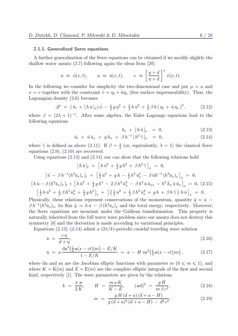
Figure 2. Two exact solutions to the Serre equations. The solitary waveamplitude is equal to a = 0.05. For the cnoidal wave parametersm and a are equal to 0.99 and 0.05 respectively. Other cnoidalwave parameters are deduced from relations (2.18), (2.19).
However, in the present study, we are interested in the classical solitary wave solutionwhich is recovered in the limiting case m→ 1
η = a sech2 12κ(x− ct), u =
c η
d+ η, c2 = g(d+ a), (κd)2 =
a
β(d+ a). (2.20)
For illustrative purposes, a solitary wave along with a cnoidal wave of the same amplitudea = 0.05 are depicted in Figure 2.
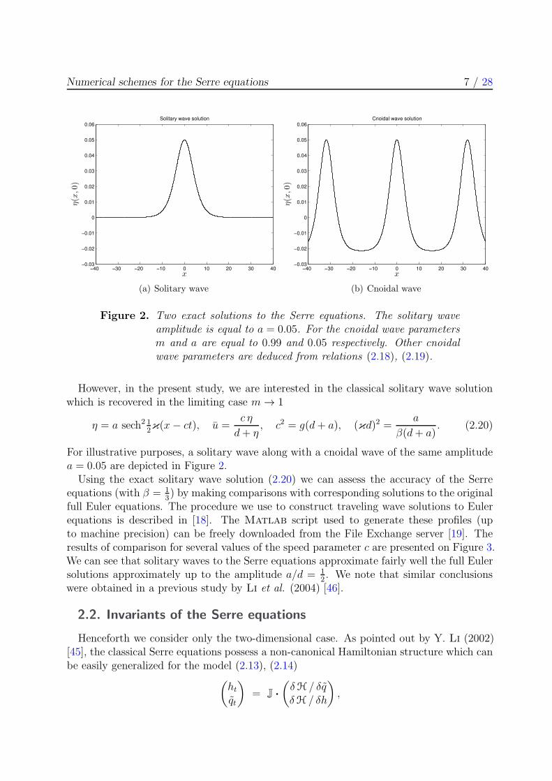
Using the exact solitary wave solution (2.20) we can assess the accuracy of the Serreequations (with β = 1
3) by making comparisons with corresponding solutions to the original
full Euler equations. The procedure we use to construct traveling wave solutions to Eulerequations is described in [18]. The Matlab script used to generate these profiles (upto machine precision) can be freely downloaded from the File Exchange server [19]. Theresults of comparison for several values of the speed parameter c are presented on Figure 3.We can see that solitary waves to the Serre equations approximate fairly well the full Eulersolutions approximately up to the amplitude a/d = 1
2. We note that similar conclusions
were obtained in a previous study by Li et al. (2004) [46].
2.2. Invariants of the Serre equations
Henceforth we consider only the two-dimensional case. As pointed out by Y. Li (2002)[45], the classical Serre equations possess a non-canonical Hamiltonian structure which canbe easily generalized for the model (2.13), (2.14)
(htqt
)
= J ·
(δH / δqδH / δh
)
,
D. Dutykh, D. Clamond, P. Milewski & D. Mitsotakis 8 / 28
−10 −8 −6 −4 −2 0 2 4 6 8 100
0.1
0.2
0.3
0.4
0.5
0.6
x/d
η(x,0
)/d
Euler
Serre
(a) c = 1.1
−10 −8 −6 −4 −2 0 2 4 6 8 100
0.1
0.2
0.3
0.4
0.5
0.6
x/d
η(x,0
)/d
Euler
Serre
(b) c = 1.15
−10 −8 −6 −4 −2 0 2 4 6 8 100
0.1
0.2
0.3
0.4
0.5
0.6
x/d
η(x,0
)/d
Euler
Serre
(c) c = 1.2
−10 −8 −6 −4 −2 0 2 4 6 8 10
0
0.1
0.2
0.3
0.4
0.5
0.6
x/d
η(x,0
)/d
Euler
Serre
(d) c = 1.25
Figure 3. Comparison of solitary wave solutions to the Serre and the fullEuler equations.
where the Hamiltonian functional H and the symplectic operator J are defined as
H = 12
ˆ
R
[h u2 + β h3 u2x + g η2
]dx, J = −
[hx 0
qx + q∂x h∂x
]
.
The variable q is defined by
q ≡ h u − β [ h3 ux ]x.
The conservation of the quantity q was established in equation (2.15).According to [45], one-parameter symmetry groups of Serre’s equations include the space
translation (x + ε, t, h, u), the time translation (x, t + ε, h, u), the Galilean boost (x +εt, t, h, u+ ε) and the scaling eε(eεx, t, eεh, u). Using the first three symmetry groups and
Numerical schemes for the Serre equations 9 / 28
the symplectic operator J, one may recover the following invariants:
Q =
ˆ
R
η q
d + ηdx, H,
ˆ
R
[ t q − x η ] dx. (2.21)
Obviously, the equation (2.13) leads to an invariant closely related to the mass conservationproperty
´
Rη dx. The scaling does not yield any conserved quantity with respect to the
symplectic operator J. Below, we are going to use extensively the generalized energy H
and the generalized momentum Q conservation to assess the accuracy of the numericalschemes in addition to the exact analytical solution (2.20).
3. Finite volume scheme and numerical results
In the present study, we propose a finite volume discretization procedure [5, 6] for theSerre equations (2.13), (2.14) that we rewrite here as
ht + [ h u ]x = 0, (3.1)
ut +[
12u2 + g h
]
x= β h−1
[h3 (uxt + u uxx − u 2
x)]
x, (3.2)
where the over-bars have been omitted for brevity. (In this section, over-bars denotequantities averaged over a cell, as explained below.)
We begin our presentation by a discretization of the hyperbolic part of the equations(which are simply the classical Saint-Venant equations) and then discuss the treatment ofdispersive terms. The Serre equations can be formally put under the quasilinear form
V t + [F (V ) ]x = S(V ), (3.3)
where V , F (V ) are the conservative variables and the advective flux function, respectively
V ≡(hu
)
, F (V ) ≡(
h u12u2 + g h
)
.
The source term S(V ) denotes the right-hand side of (3.1), (3.2) and thus, depends alsoon space and time derivatives of V . The Jacobian of the advective flux F (V ) can be easilycomputed
A(V ) =∂ F (V )
∂V=
[u hg u
]
.
The Jacobian A(V ) has two distinctive eigenvalues
λ± = u ± cs, cs ≡√
gh.
The corresponding right and left eigenvectors are provided here
R =
[h −hcs cs
]
, L = R−1 =
1
2
[h−1 c−1
s
−h−1 c−1s
]
.
We consider a partition of the real line R into cells (or finite volumes) Ci = [xi− 1
2
, xi+ 1
2
]
with cell centers xi =12(xi− 1
2
+ xi+ 1
2
) (i ∈ Z). Let ∆xi denotes the length of the cell Ci. In
the sequel we will consider only uniform partitions with ∆xi = ∆x, ∀i ∈ Z. We would like
D. Dutykh, D. Clamond, P. Milewski & D. Mitsotakis 10 / 28
to approximate the solution V (x, t) by discrete values. In order to do so, we introduce thecell average of V on the cell Ci (denoted with an overbar), i.e.,
V i(t) ≡(hi(t) , ui(t)
)=
1
∆x
ˆ
Ci
V (x, t) dx.
A simple integration of (3.3) over the cell Ci leads the following exact relation:
d V
dt+
1
∆x
[
F (V (xi+ 1
2
, t)) − F (V (xi− 1
2
, t))]
=1
∆x
ˆ
Ci
S(V ) dx ≡ Si.
Since the discrete solution is discontinuous at cell interfaces xi+ 1
2
(i ∈ Z), we replace the
flux at the cell faces by the so-called numerical flux function
F (V (xi± 1
2
, t)) ≈ Fi± 1
2
(VL
i± 1
2
, VR
i± 1
2
),
where VL,R
i± 1
2
denotes the reconstructions of the conservative variables V from left and right
sides of each cell interface (the reconstruction procedure employed in the present studywill be described below). Consequently, the semi-discrete scheme takes the form
d V i
dt+
1
∆x
[
Fi+ 1
2
− Fi− 1
2
]
= Si. (3.4)
In order to discretize the advective flux F (V ), we use the FVCF scheme [36, 37]:
F(V ,W ) =F (V ) + F (W )
2− U(V ,W ) ·
F (W ) − F (V )
2.
The first part of the numerical flux is centered, the second part is the upwinding introducedthrough the Jacobian sign-matrix U(V ,W ) defined as
U(V ,W ) = sign[A(12(V +W )
)], sign(A) = R · diag(s+, s−) · L,
where s± ≡ sign(λ±). After some simple algebraic computations, one can find
U =1
2
[s+ + s− (h/cs) (s
+ − s−)(g/cs) (s
+ − s−) s+ + s−
]
,
the sign-matrix U being evaluated at the average state of left and right values.
3.1. High order reconstruction
In order to obtain a higher-order scheme in space, we need to replace the piecewiseconstant data by a piecewise polynomial representation. This goal is achieved by variousso-called reconstruction procedures such as MUSCL TVD [43, 66, 67], UNO [40], ENO [39],WENO [72] and many others. In our previous study on Boussinesq-type equations [32], theUNO2 scheme showed a good performance with small dissipation in realistic propagationand run-up simulations. Consequently, we retain this scheme for the discretization of theadvective flux in Serre equations.
Remark 4. In TVD schemes, the numerical operator is required (by definition) not toincrease the total variation of the numerical solution at each time step. It follows that thevalue of an isolated maximum may only decrease in time which is not a good property forthe simulation of coherent structures such as solitary waves. The non-oscillatory UNO2
Numerical schemes for the Serre equations 11 / 28
scheme, employed in our study, is only required to diminish the number of local extrema inthe numerical solution. Unlike TVD schemes, UNO schemes are not constrained to dampthe values of each local extremum at every time step.
The main idea of the UNO2 scheme is to construct a non-oscillatory piecewise-parabolicinterpolant Q(x) to a piecewise smooth function V (x) (see [40] for more details). On eachsegment containing the face xi+ 1
2
∈ [xi, xi+1], the function Q(x) = qi+ 1
2
(x) is locally a
quadratic polynomial and wherever v(x) is smooth we have
Q(x) − V (x) = 0 + O(∆x3),dQ
dx(x± 0) − dV
dx= 0 + O(∆x2).
Also, Q(x) should be non-oscillatory in the sense that the number of its local extrema doesnot exceed that of V (x). Since qi+ 1
2
(xi) = V i and qi+ 1
2
(xi+1) = V i+1, it can be written in
the form
qi+ 1
2
(x) = V i + di+ 1
2
V × x− xi∆x
+ 12Di+ 1
2
V × (x− xi)(x− xi+1)
∆x2,
where di+ 1
2
V ≡ V i+1−V i and Di+ 1
2
V is closely related to the second derivative of the in-
terpolant since Di+ 1
2
V = ∆x2 q′′
i+ 1
2
(x). The polynomial qi+ 1
2
(x) is chosen to be the least
oscillatory between two candidates interpolating V (x) at (xi−1, xi, xi+1) and (xi, xi+1, xi+2).This requirement leads to the following choice of Di+ 1
2
V ≡ minmod (DiV ,Di+1V )with
DiV = V i+1 − 2 V i + V i−1, Di+1V = V i+2 − 2 V i+1 + V i,
and where minmod(x, y) is the usual minmod function defined as
minmod(x, y) ≡ 12[ sign(x) + sign(y) ]×min(|x|, |y|).
To achieve the second order O(∆x2) accuracy, it is sufficient to consider piecewise linearreconstructions in each cell. Let L(x) denote this approximately reconstructed functionwhich can be written in this form
L(x) = V i + Si ×x− xi∆x
, x ∈ [xi− 1
2
, xi+ 1
2
].
In order to L(x) be a non-oscillatory approximation, we use the parabolic interpolationQ(x) constructed below to estimate the slopes Si within each cell
Si = ∆x×minmod
(dQ
dx(xi − 0),
dQ
dx(xi + 0)
)
.
In other words, the solution is reconstructed on the cells while the solution gradient isestimated on the dual mesh as it is often performed in more modern schemes [5, 6]. A briefsummary of the UNO2 reconstruction can be also found in [32, 33].
3.2. Treatment of the dispersive terms
In this section, we explain how we treat the dispersive terms of Serre equations (3.1),(3.2). We begin the exposition by discussing the space discretization and then, we proposea way to remove the intrinsic stiffness of the dispersion by partial implicitation.
D. Dutykh, D. Clamond, P. Milewski & D. Mitsotakis 12 / 28
For the sake of simplicity, we split the dispersive terms into three parts:
M(V ) ≡ β h−1[h3 uxt
]
x, D1(V ) ≡ β h−1
[h3 u uxx
]
x, D2(V ) ≡ β h−1
[h3 u 2
x
]
x.
We propose the following approximations in space (which are all of the second order O(∆x2)to be consistent with UNO2 advective flux discretization presented above)
Mi(V ) = β h−1i
h3i+1 (uxt)i+1 − h
3i−1 (uxt)i−1
2∆x
=β h
−1i
2∆x
[
h3i+1
(ut)i+2 − (ut)i2∆x
− h3i−1
(ut)i − (ut)i−2
2∆x
]
=β h
−1i
4∆x2
[
h3i+1 (ut)i+2 − (h
3i+1 + h
3i−1) (ut)i + h
3i−1 (ut)i−2
]
.
The last relation can be rewritten in a short-hand form if we introduce the matrix M(V )such that the i-th component of the product M(V )·V t gives exactly the expression Mi(V ).
In a similar way, we discretize the other dispersive terms without giving here the inter-mediate steps
D1i(V ) =β h
−1i
2∆x3
[
h3i+1 ui+1 (ui+2 − 2ui+1 + ui) − h
3i−1 ui−1 (ui − 2ui−1 + ui−2)
]
,
D2i(V ) =βh
−1i
8∆x3
[
h3i+1 (ui+2 − ui)
2 − h3i−1 (ui − ui−2)
2]
.
In a more general nonperiodic case asymmetric finite differences should be used near theboundaries. If we denote by I the identity matrix, we can rewrite the semi-discrete scheme(3.4) by expanding the right-hand side Si
d h
dt+
1
∆x
[
F(1)+ (V ) − F
(1)− (V )
]
= 0, (3.5)
(I−M) · d udt
+1
∆x
[
F(2)+ (V ) − F
(2)− (V )
]
= D(V ) · u, (3.6)
where F(1,2)± (V ) are the two components of the advective numerical flux vector F at the
right (+) and left (−) faces correspondingly and D(V ) ≡ D1(V )− D2(V ).Finally, in order to obtain the semidiscrete scheme, one has to solve a linear system to
find explicitly the time derivative du/dt. A mathematical study of the resulting matrixI − M is not straightforward to perform. However, in our numerical tests we have neverexperienced any difficulties to invert it.
3.3. Temporal scheme
We rewrite the inverted semi-discrete scheme (3.5)–(3.6) as a system of ODEs:
∂t w = L(w, t), w(0) = w0.
In order to solve numerically the last system of equations, we apply the Bogacki–Shampinemethod [9]. It is a third-order Runge–Kutta scheme with four stages. It has an embeddedsecond-order method which is used to estimate the local error and, thus, to adapt thetime step size. Moreover, the Bogacki–Shampine method enjoys the First Same As Last
Numerical schemes for the Serre equations 13 / 28
(FSAL) property so that it needs three function evaluations per step. This method is alsoimplemented in the ode23 function in Matlab [60]. A step of the Bogacki–Shampinemethod is given by
k1 = L(w(n), tn),
k2 = L(w(n) + 12∆tnk1, tn +
12∆t),
k3 = L(w(n)) + 34∆tnk2, tn +
34∆t),
w(n+1) = w(n) + ∆tn ×(29k1 +
13k2 +
49k3),
k4 = L(w(n+1), tn +∆tn),
w(n+1)2 = w(n) + ∆tn ×
(424k1 +
14k2 +
13k3 +
18k4).
Here w(n) ≈ w(tn), ∆t is the time step and w(n+1)2 is a second order approximation to the
solution w(tn+1), so the difference between w(n+1) and w(n+1)2 gives an estimation of the
local error. The FSAL property consists in the fact that k4 is equal to k1 in the next timestep, thus saving one function evaluation.
If the new time step ∆tn+1 is given by ∆tn+1 = ρn∆tn, then according to H211b digitalfilter approach [61, 62], the proportionality factor ρn is given by:
ρn =
(δ
εn
)β1(
δ
εn−1
)β2
ρ−αn−1, (3.7)
where εn is a local error estimation at time step tn, δ is the desired tolerance and theconstants β1, β2 and α are defined as
α =1
4, β1 = β2 =
1
4 p.
The parameter p is the order of the scheme (p = 3 in our case).
Remark 5. The adaptive strategy (3.7) can be further improved if we smooth the factorρn before computing the next time step ∆tn+1
∆tn+1 = ρn ∆tn, ρn = ω(ρn).
The function ω(ρ) is called the time step limiter and should be smooth, monotonicallyincreasing and should satisfy the following conditions
ω(0) < 1, ω(+∞) > 1, ω(1) = 1, ω′(1) = 1.
One possible choice is suggested in [62]:
ω(ρ) = 1 + κ arctan
(ρ− 1
κ
)
.
In our computations the parameter κ is set to 1.
D. Dutykh, D. Clamond, P. Milewski & D. Mitsotakis 14 / 28
4. Pseudo-spectral Fourier-type method for the Serre
equations
In this Section we describe a pseudo-spectral solver to integrate numerically the Serreequations in periodic domains. In spectral methods, it is more convenient to take asvariables the free surface elevation η(x, t) and the conserved quantity q(x, t)
ηt + [ (d+ η) u ]x = 0, (4.1)
qt +[q u − 1
2u2 + g η − 1
2(d+ η)2 u2x
]
x= 0, (4.2)
q − u + 13(d+ η)2uxx + (d+ η)ηxux = 0. (4.3)
The first two equations (4.1), (4.2) are of evolution type, while the third one (4.3) relatesthe conserved variable q to the primitive variables: the free surface elevation η and thevelocity u. In order to solve relation (4.3) with respect to the velocity u, we extract thelinear part as
u − 13d2 uxx − q = 1
3(2dη + η2) uxx + (d+ η) ηx ux
︸ ︷︷ ︸
N(η,u)
.
Then, we apply to the last relation the following fixed point type iteration in Fourier space
ˆuj+1 =q
1 + 13(kd)2
+F N(η, uj)1 + 1
3(kd)2
j = 0, 1, 2, · · · , (4.4)
where ψ ≡ Fψ denotes the Fourier transform of a quantity ψ. The last iteration isrepeated until the desired convergence. For example, for moderate amplitude solitary waves(≈ 0.2), the accuracy 10−16 is attained in approximatively 20 iterations if the velocity u0 isinitialized from the previous time step. We note that the usual 3/2 rule is applied to thenonlinear terms for anti-aliasing [65, 21, 35].
Remark 6. One can improve the fixed point iteration (4.4) by employing the so-calledrelaxation approach [41]. The relaxed scheme takes the following form
ˆuj+1 =
(q
1 + 13(kd)2
+F N(η, uj)1 + 1
3(kd)2
)
θ + (1− θ)ˆuj j = 0, 1, 2, · · · ,
where θ ∈ [0, 1] is a free parameter. We obtained the best convergence rate for θ = 12.
In order to improve the numerical stability of the time stepping method, we will integrateexactly the linear terms in evolution equations
ηt + d ux = −[ η u ]x,
qt + g ηx =[
12u2 + 1
2(d+ η)2 u2x − q u
]
x.
Taking the Fourier transform and using the relation (4.3) between u and q, we obtain thefollowing system of ODEs:
ηt +ikd
1 + 13(kd)2
q = −ik Fηu − ikdF N(η, uj)1 + 1
3(kd)2
,
qt + ikg η = ik F
12u2 + 1
2(d+ η)2u2x − qu
.
Numerical schemes for the Serre equations 15 / 28
The next step consists in introducing the vector of dimensionless variables in Fourier spaceV ≡ (ikη, iωq/g), where ω2 = gk2d/[1 + 1
3(kd)2] is the dispersion relation of the linearized
Serre equations. With unscaled variables in vectorial form, the last system becomes
V t + L · V = N(V ), L ≡[0 iωiω 0
]
.
On the right-hand side, we put all the nonlinear terms
N(V ) =
(k2 Fηu + dk2 F N(η, uj) /(1 + 1
3(kd)2)
−(kω/g)F
12u2 + 1
2(d+ η)2u2x − qu
)
.
In order to integrate the linear terms, we make a last change of variables [51, 35]:
W t = e(t−t0)L ·N
e−(t−t0)L · W
, W (t) ≡ e(t−t0)L · V (t), W (t0) = V (t0).
Finally, the last system of ODEs is discretized in time by Verner’s embedded adaptive9(8) Runge–Kutta scheme [68]. The time step is chosen adaptively using the so-calledH211b digital filter [61, 62] to meet some prescribed error tolerance (generally of the sameorder of the fixed point iteration (4.4) precision). Since the numerical scheme is implicitin the velocity variable u, the resulting time step ∆t is generally of the order of the spatialdiscretization O(∆x).
5. Numerical results
In this section we present some numerical results using the finite volume scheme describedhereinabove. First, we validate the discretization and check the convergence of the schemeusing an analytical solution. Then we demonstrate the ability of the scheme to simulatethe practically important solitary wave interaction problem. Throughout this section weconsider the initial value problem with periodic boundary conditions unless a special remarkis made.
5.1. Convergence test and invariants preservation
Consider the Serre equations (3.1), (3.2) posed in the periodic domain [−40, 40]. Wesolve numerically the initial-periodic boundary value problem with an exact solitary wavesolution (2.20) posed as an initial condition. Then, this specific initial disturbance will betranslated in space with known celerity under the system dynamics. This particular classof solutions plays an important role in water wave theory [29, 28] and it will allow us toassess the accuracy of the proposed scheme. The values of the various physical parametersused in the simulation are given in Table 1.
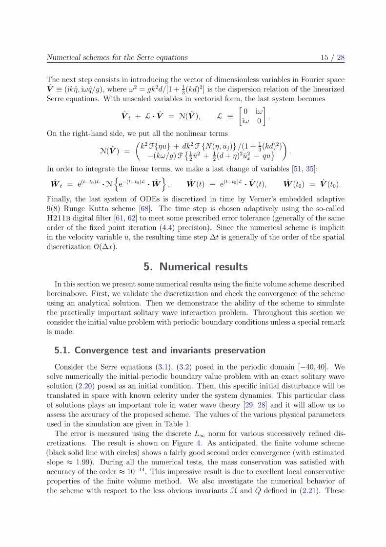
The error is measured using the discrete L∞ norm for various successively refined dis-cretizations. The result is shown on Figure 4. As anticipated, the finite volume scheme(black solid line with circles) shows a fairly good second order convergence (with estimatedslope ≈ 1.99). During all the numerical tests, the mass conservation was satisfied withaccuracy of the order ≈ 10−14. This impressive result is due to excellent local conservativeproperties of the finite volume method. We also investigate the numerical behavior ofthe scheme with respect to the less obvious invariants H and Q defined in (2.21). These
D. Dutykh, D. Clamond, P. Milewski & D. Mitsotakis 16 / 28
Undisturbed water depth: d 1Gravity acceleration: g 1Solitary wave amplitude: a 0.05Final simulation time: T 2Free parameter: β 1/3
Table 1. Values of various parameters used in convergence tests.
101
102
103
10−6
10−5
10−4
10−3
10−2
10−1
N
L∞
error
FV UNO2
N−2
N−1
Figure 4. Convergence of the numerical solution in the L∞ norm computedusing the finite volume method.
invariants can be computed exactly for solitary waves. However, we do not provide themto avoid cumbersome expressions. For the solitary wave with parameters given in Table 1,the generalized energy and momentum are given by the following expressions:
H0 =21√7
100+
7√3
10log
√21− 1√21 + 1
≈ 0.0178098463,
Q0 =62√15
225+
2√35
5log
√21− 1√21 + 1
≈ 0.017548002.
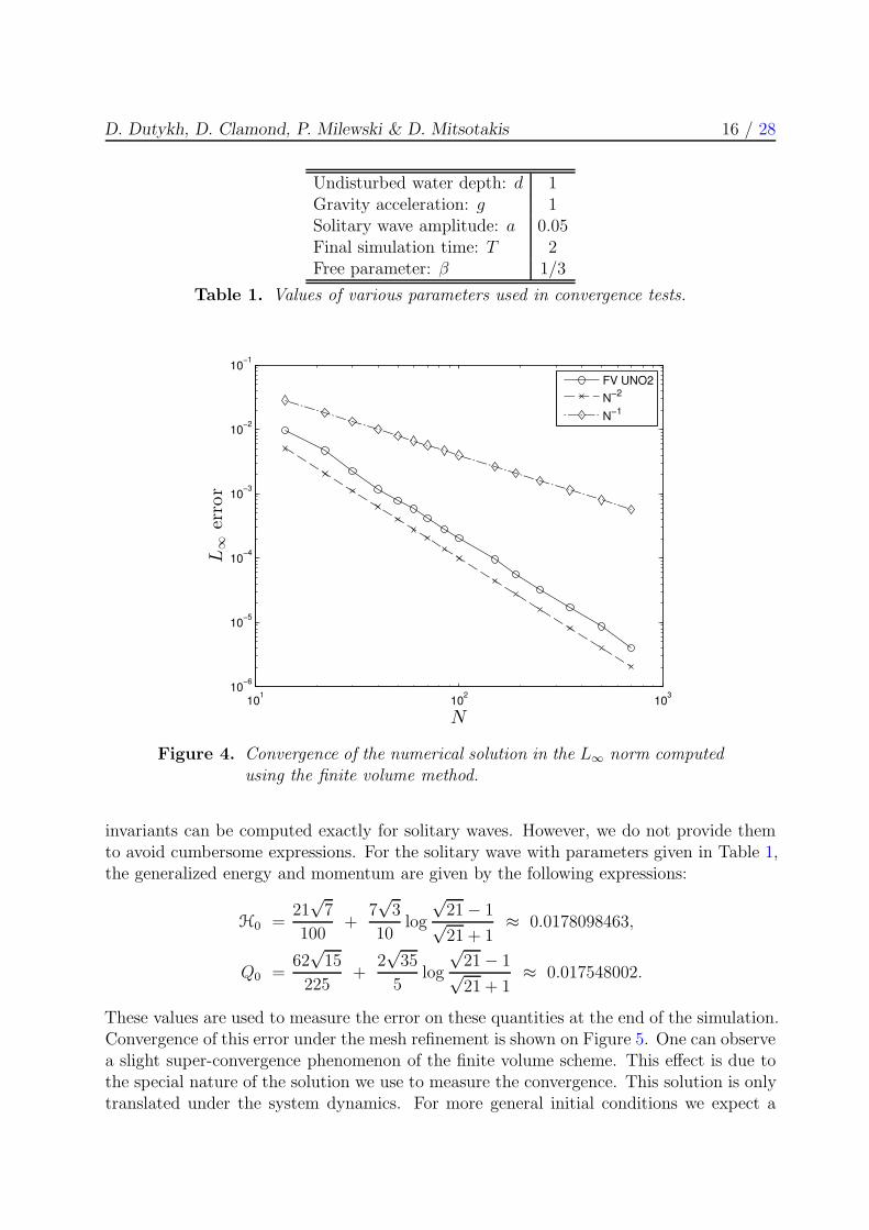
These values are used to measure the error on these quantities at the end of the simulation.Convergence of this error under the mesh refinement is shown on Figure 5. One can observea slight super-convergence phenomenon of the finite volume scheme. This effect is due tothe special nature of the solution we use to measure the convergence. This solution is onlytranslated under the system dynamics. For more general initial conditions we expect a
Numerical schemes for the Serre equations 17 / 28
101
102
103
10−8
10−7
10−6
10−5
10−4
10−3
10−2
N
|H(T
)−
H0|
Error
N−2
Spectral
(a) Hamiltonian H
101
102
103
10−8
10−7
10−6
10−5
10−4
10−3
10−2
N|Q
(T)−
Q0|
Error
N−2
Spectral
(b) Momentum Q
Figure 5. Hamiltonian and generalized momentum conservation conver-gence computed using the finite volume and spectral methods un-der the mesh refinement. The conserved quantities are measuredat the final simulation time.
fair theoretical 2 nd order convergence for the finite volume scheme. As anticipated, thepseudo-spectral scheme shows the exponential error decay.
5.2. Solitary wave interaction
Solitary wave interactions are an important phenomenon in nonlinear dispersive waveswhich have been studied by numerical and analytical methods and results have been com-pared to experimental evidence. They also often serve as one of the most robust nonlinearbenchmark test cases for numerical methods. We mention only a few works among theexisting literature. For example, in [48, 56, 23] solitary wave interactions were studiedexperimentally. The head-on collision of solitary waves was studied in the framework offull Euler equations in [23, 14]. Studies of solitary waves in various approximate modelscan be found in [46, 26, 2, 32, 33]. To our knowledge, solitary wave collisions for the Serreequations were studied numerically for the first time in the PhD thesis of Seabra-Santos[57]. Finally, there are also a few studies devoted to simulations with full Euler equations[46, 35, 23].
5.2.1. Head-on collision
Consider the Serre equations posed in the domain [−40, 40] with periodic boundaryconditions. In the present section, we study the head-on collision (weak interaction) oftwo solitary waves of equal amplitude moving in opposite directions. Initially, two solitarywaves of amplitude a = 0.15 are located at x0 = ±20 (other parameters can be found inTable 1). The computational domain is divided into N = 1000 intervals (finite volumesin 1D) of the uniform length ∆x = 0.08. The time step is chosen to be ∆t ≈ 10−3. The
D. Dutykh, D. Clamond, P. Milewski & D. Mitsotakis 18 / 28
−40
−20
0
20
40
0
10
20
30
40
−0.1
0
0.1
0.2
0.3
0.4
tx
η(x,t)
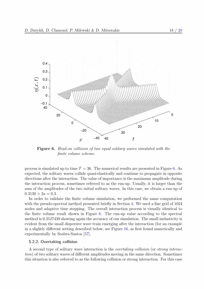
Figure 6. Head-on collision of two equal solitary waves simulated with thefinite volume scheme.
process is simulated up to time T = 36. The numerical results are presented in Figure 6. Asexpected, the solitary waves collide quasi-elastically and continue to propagate in oppositedirections after the interaction. The value of importance is the maximum amplitude duringthe interaction process, sometimes referred to as the run-up. Usually, it is larger than thesum of the amplitudes of the two initial solitary waves. In this case, we obtain a run-up of0.3130 > 2a = 0.3.
In order to validate the finite volume simulation, we performed the same computationwith the pseudo-spectral method presented briefly in Section 4. We used a fine grid of 1024nodes and adaptive time stepping. The overall interaction process is visually identical tothe finite volume result shown in Figure 6. The run-up value according to the spectralmethod is 0.3127439 showing again the accuracy of our simulation. The small inelasticity isevident from the small dispersive wave train emerging after the interaction (for an examplein a slightly different setting described below, see Figure 16, as first found numerically andexperimentally by Seabra-Santos [57].
5.2.2. Overtaking collision
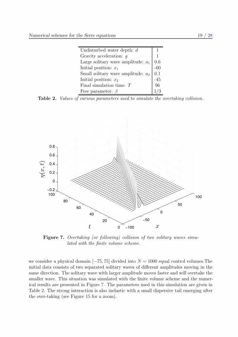
A second type of solitary wave interaction is the overtaking collision (or strong interac-tion) of two solitary waves of different amplitudes moving in the same direction. Sometimesthis situation is also referred to as the following collision or strong interaction. For this case
Numerical schemes for the Serre equations 19 / 28
Undisturbed water depth: d 1Gravity acceleration: g 1Large solitary wave amplitude: a1 0.6Initial position: x1 -60Small solitary wave amplitude: a2 0.1Initial position: x2 -45Final simulation time: T 96Free parameter: β 1/3
Table 2. Values of various parameters used to simulate the overtaking collision.
−100
−50
0
50
100
0
20
40
60
80
100
−0.2
0
0.2
0.4
0.6
0.8
xt
η(x,t)
Figure 7. Overtaking (or following) collision of two solitary waves simu-lated with the finite volume scheme.
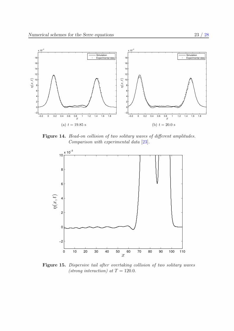
we consider a physical domain [−75, 75] divided into N = 1000 equal control volumes.Theinitial data consists of two separated solitary waves of different amplitudes moving in thesame direction. The solitary wave with larger amplitude moves faster and will overtake thesmaller wave. This situation was simulated with the finite volume scheme and the numer-ical results are presented in Figure 7. The parameters used in this simulation are given inTable 2. The strong interaction is also inelastic with a small dispersive tail emerging afterthe over-taking (see Figure 15 for a zoom).
D. Dutykh, D. Clamond, P. Milewski & D. Mitsotakis 20 / 28
−0.2 0 0.2 0.4 0.6 0.8 1 1.2 1.4 1.6 1.8
−2
0
2
4
6
8
10
12
14
16
18
x 10−3
x
η(x,t)
Simulation
Experimental data
(a) t = 18.5 s
−0.2 0 0.2 0.4 0.6 0.8 1 1.2 1.4 1.6 1.8
−2
0
2
4
6
8
10
12
14
16
18
x 10−3
xη(x,t)
Simulation
Experimental data
(b) t = 18.6 s
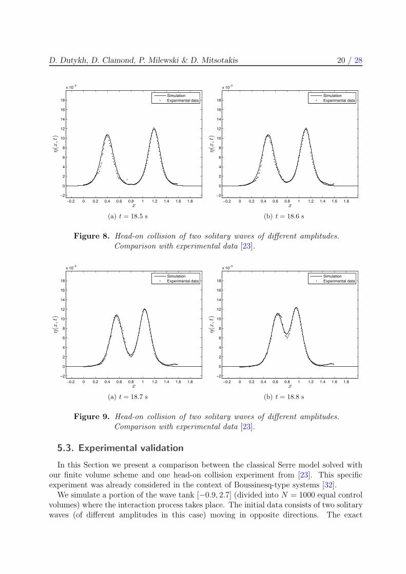
Figure 8. Head-on collision of two solitary waves of different amplitudes.Comparison with experimental data [23].
−0.2 0 0.2 0.4 0.6 0.8 1 1.2 1.4 1.6 1.8
−2
0
2
4
6
8
10
12
14
16
18
x 10−3
x
η(x,t)
Simulation
Experimental data
(a) t = 18.7 s
−0.2 0 0.2 0.4 0.6 0.8 1 1.2 1.4 1.6 1.8
−2
0
2
4
6
8
10
12
14
16
18
x 10−3
x
η(x,t)
Simulation
Experimental data
(b) t = 18.8 s
Figure 9. Head-on collision of two solitary waves of different amplitudes.Comparison with experimental data [23].
5.3. Experimental validation
In this Section we present a comparison between the classical Serre model solved withour finite volume scheme and one head-on collision experiment from [23]. This specificexperiment was already considered in the context of Boussinesq-type systems [32].
We simulate a portion of the wave tank [−0.9, 2.7] (divided into N = 1000 equal controlvolumes) where the interaction process takes place. The initial data consists of two solitarywaves (of different amplitudes in this case) moving in opposite directions. The exact
Numerical schemes for the Serre equations 21 / 28
−0.2 0 0.2 0.4 0.6 0.8 1 1.2 1.4 1.6 1.8
−2
0
2
4
6
8
10
12
14
16
18
x 10−3
x
η(x,t)
Simulation
Experimental data
(a) t = 18.92 s
−0.2 0 0.2 0.4 0.6 0.8 1 1.2 1.4 1.6 1.8
0
0.005
0.01
0.015
0.02
0.025
xη(x,t)
Simulation
Experimental data
(b) t = 19.0 s
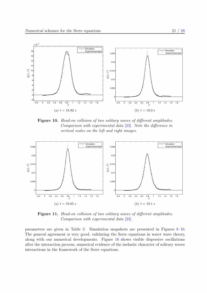
Figure 10. Head-on collision of two solitary waves of different amplitudes.Comparison with experimental data [23]. Note the difference invertical scales on the left and right images.
−0.2 0 0.2 0.4 0.6 0.8 1 1.2 1.4 1.6 1.8
0
0.005
0.01
0.015
0.02
0.025
x
η(x,t)
Simulation
Experimental data
(a) t = 19.05 s
−0.2 0 0.2 0.4 0.6 0.8 1 1.2 1.4 1.6 1.8
0
0.005
0.01
0.015
0.02
0.025
x
η(x,t)
Simulation
Experimental data
(b) t = 19.1 s
Figure 11. Head-on collision of two solitary waves of different amplitudes.Comparison with experimental data [23].
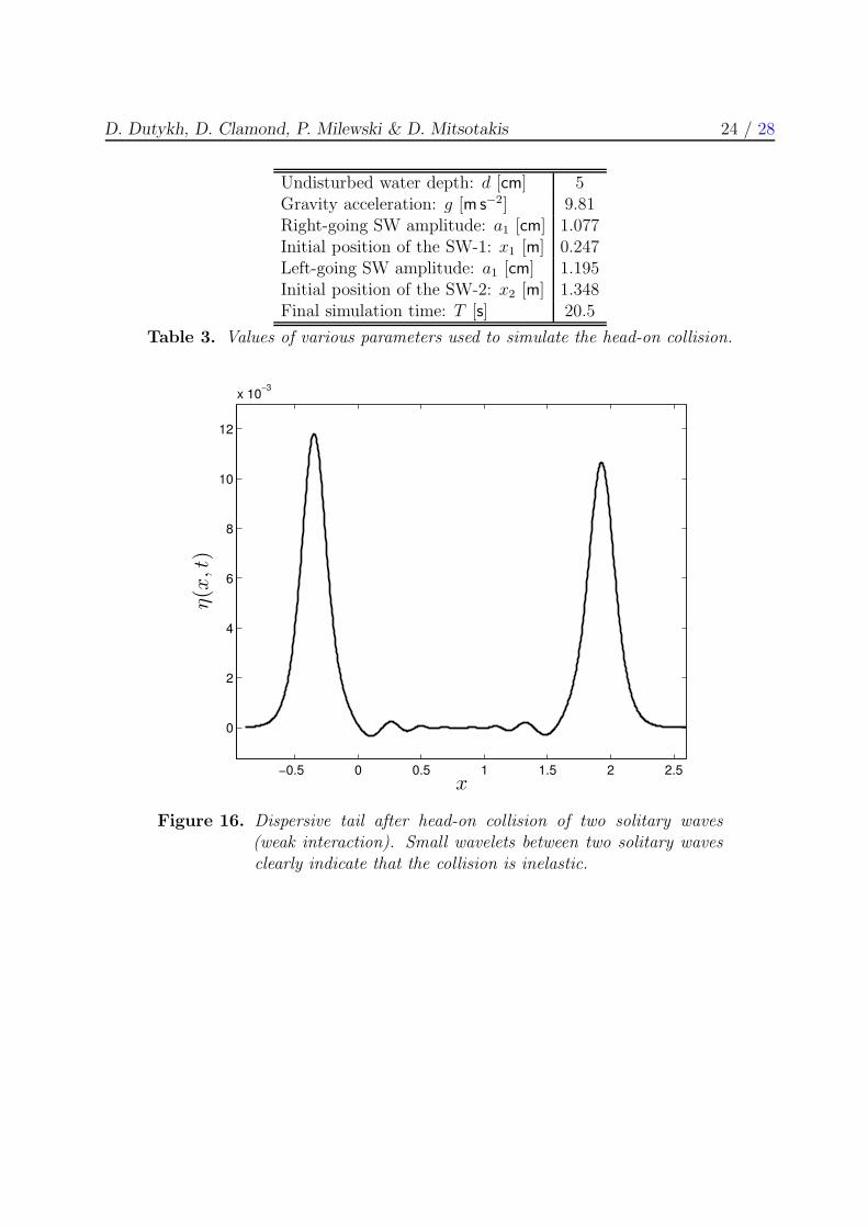
parameters are given in Table 3. Simulation snapshots are presented in Figures 8–16.The general agreement is very good, validating the Serre equations in water wave theory,along with our numerical developments. Figure 16 shows visible dispersive oscillationsafter the interaction process, numerical evidence of the inelastic character of solitary wavesinteractions in the framework of the Serre equations.
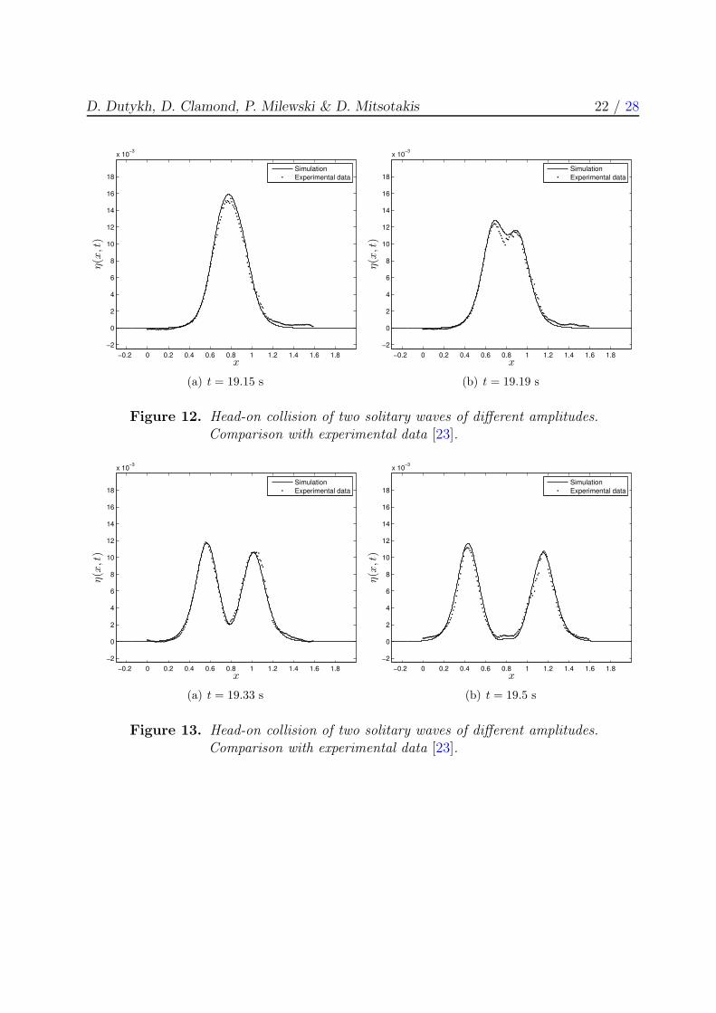
D. Dutykh, D. Clamond, P. Milewski & D. Mitsotakis 22 / 28
−0.2 0 0.2 0.4 0.6 0.8 1 1.2 1.4 1.6 1.8
−2
0
2
4
6
8
10
12
14
16
18
x 10−3
x
η(x,t)
Simulation
Experimental data
(a) t = 19.15 s
−0.2 0 0.2 0.4 0.6 0.8 1 1.2 1.4 1.6 1.8
−2
0
2
4
6
8
10
12
14
16
18
x 10−3
xη(x,t)
Simulation
Experimental data
(b) t = 19.19 s
Figure 12. Head-on collision of two solitary waves of different amplitudes.Comparison with experimental data [23].
−0.2 0 0.2 0.4 0.6 0.8 1 1.2 1.4 1.6 1.8
−2
0
2
4
6
8
10
12
14
16
18
x 10−3
x
η(x,t)
Simulation
Experimental data
(a) t = 19.33 s
−0.2 0 0.2 0.4 0.6 0.8 1 1.2 1.4 1.6 1.8
−2
0
2
4
6
8
10
12
14
16
18
x 10−3
x
η(x,t)
Simulation
Experimental data
(b) t = 19.5 s
Figure 13. Head-on collision of two solitary waves of different amplitudes.Comparison with experimental data [23].
Numerical schemes for the Serre equations 23 / 28
−0.2 0 0.2 0.4 0.6 0.8 1 1.2 1.4 1.6 1.8
−2
0
2
4
6
8
10
12
14
16
18
x 10−3
x
η(x,t)
Simulation
Experimental data
(a) t = 19.85 s
−0.2 0 0.2 0.4 0.6 0.8 1 1.2 1.4 1.6 1.8
−2
0
2
4
6
8
10
12
14
16
18
x 10−3
xη(x,t)
Simulation
Experimental data
(b) t = 20.0 s
Figure 14. Head-on collision of two solitary waves of different amplitudes.Comparison with experimental data [23].
0 10 20 30 40 50 60 70 80 90 100 110
−2
0
2
4
6
8
10x 10
−3
x
η(x,t)
Figure 15. Dispersive tail after overtaking collision of two solitary waves(strong interaction) at T = 120.0.
D. Dutykh, D. Clamond, P. Milewski & D. Mitsotakis 24 / 28
Undisturbed water depth: d [cm] 5Gravity acceleration: g [ms
−2] 9.81Right-going SW amplitude: a1 [cm] 1.077Initial position of the SW-1: x1 [m] 0.247Left-going SW amplitude: a1 [cm] 1.195Initial position of the SW-2: x2 [m] 1.348Final simulation time: T [s] 20.5
Table 3. Values of various parameters used to simulate the head-on collision.
−0.5 0 0.5 1 1.5 2 2.5
0
2
4
6
8
10
12
x 10−3
x
η(x,t)
Figure 16. Dispersive tail after head-on collision of two solitary waves(weak interaction). Small wavelets between two solitary wavesclearly indicate that the collision is inelastic.
Numerical schemes for the Serre equations 25 / 28
6. Conclusions
The current study is devoted to the Serre equations stemming from water wave modeling[59, 7, 25]. First, we presented a derivation of this model using a relaxed variationalprinciple [20]. We then described an Implicit-Explicit finite volume scheme to discretizethe equations. The overall theoretical accuracy of the discretization scheme is of second-order. This conclusion is confirmed by comparisons with an exact solitary wave solution.The energy conservation properties of our scheme are also discussed and quantified. Inorder to validate further our numerical scheme, we present a Fourier-type pseudo-spectralmethod. Both numerical methods are compared on solitary wave interaction problems.The proposed discretization procedure was successfully validated with several numericaltests along with experimental data. In contrast with the highly accurate spectral method,the finite volume method has the advantage of being robust and generalizable to realisticcomplex situations with variable bathymetry, very steep fronts, dry areas, etc. The presentstudy should be considered as the first step to further generalisations to 2D cartesian meshes[52, 13, 69].
Acknowledgments
D. Dutykh acknowledges the support from French “Agence Nationale de la Recherche”,project “MathOcean” (Grant ANR-08-BLAN-0301-01) along with the support from ERCunder the research project ERC-2011-AdG 290562-MULTIWAVE. P. Milewski acknowl-edges the support of the University of Savoie during his visits in 2011.
References
[1] M. Abramowitz and I. A. Stegun. Handbook of Mathematical Functions. Dover Publications, 1972. 6
[2] D. C. Antnonopoulos, V. A. Dougalis, and D. E. Mitsotakis. Initial-boundary-value problems for the
Bona-Smith family of Boussinesq systems. Advances in Differential Equations, 14:27–53, 2009. 17
[3] D. C. Antonopoulos, V. A. Dougalis, and D. E. Mitsotakis. Numerical solution of Boussinesq systems
of the Bona-Smith family. Appl. Numer. Math., 30:314–336, 2010. 2
[4] P. Avilez-Valente and F. J. Seabra-Santos. A high-order Petrov-Galerkin finite element method for
the classical Boussinesq wave model. Int. J. Numer. Meth. Fluids, 59:969–1010, 2009. 2
[5] T. J. Barth. Aspects of unstructured grids and finite-volume solvers for the Euler and Navier-Stokes
equations. Lecture series - van Karman Institute for Fluid Dynamics, 5:1–140, 1994. 9, 11
[6] T. J. Barth and M. Ohlberger. Finite volume methods: foundation and analysis. John Wiley and Sons,
Ltd, 2004. 9, 11
[7] E. Barthelemy. Nonlinear shallow water theories for coastal waves. Surveys in Geophysics, 25:315–337,
2004. 2, 25
[8] T. B. Benjamin and P. Olver. Hamiltonian structure, symmetries and conservation laws for water
waves. J. Fluid Mech, 125:137–185, 1982. 6
[9] P. Bogacki and L. F. Shampine. A 3(2) pair of Runge-Kutta formulas. Applied Mathematics Letters,
2(4):321–325, 1989. 12
[10] J. L. Bona and M. Chen. A Boussinesq system for two-way propagation of nonlinear dispersive waves.
Physica D, 116:191–224, 1998. 2
[11] L. J. F. Broer. On the Hamiltonian theory of surface waves. Applied Sci. Res., 29(6):430–446, 1974. 3
D. Dutykh, D. Clamond, P. Milewski & D. Mitsotakis 26 / 28
[12] J. D. Carter and R. Cienfuegos. The kinematics and stability of solitary and cnoidal wave solutions
of the Serre equations. Eur. J. Mech. B/Fluids, 30:259–268, 2011. 2
[13] D. M. Causon, D. M. Ingram, C. G. Mingham, G. Yang, and R. V. Pearson. Calculation of shallow
water flows using a Cartesian cut cell approach. Advances in Water Resources, 23:545–562, 2000. 25
[14] J. Chambarel, C. Kharif, and J. Touboul. Head-on collision of two solitary waves and residual falling
jet formation. Nonlin. Processes Geophys., 16:111–122, 2009. 17
[15] F. Chazel, D. Lannes, and F. Marche. Numerical simulation of strongly nonlinear and dispersive waves
using a Green-Naghdi model. J. Sci. Comput., 48:105–116, 2011. 2
[16] R. Cienfuegos, E. Barthelemy, and P. Bonneton. A fourth-order compact finite volume scheme for fully
nonlinear and weakly dispersive Boussinesq-type equations. Part I: Model development and analysis.
Int. J. Numer. Meth. Fluids, 51:1217–1253, 2006. 2
[17] R. Cienfuegos, E. Barthelemy, and P. Bonneton. A fourth-order compact finite volume scheme for
fully nonlinear and weakly dispersive Boussinesq-type equations. Part II: Boundary conditions and
model validation. Int. J. Numer. Meth. Fluids, 53:1423–1455, 2007. 2
[18] D. Clamond and D. Dutykh. Fast accurate computation of the fully nonlinear solitary surface gravity
waves. Submitted, pages 1–7, 2012. 7
[19] D. Clamond and D. Dutykh. http://www.mathworks.com/matlabcentral/fileexchange/39189-solitary-
water-wave, 2012. 7
[20] D. Clamond and D. Dutykh. Practical use of variational principles for modeling water waves. Physica
D: Nonlinear Phenomena, 241(1):25–36, 2012. 3, 4, 5, 6, 25
[21] D. Clamond and J. Grue. A fast method for fully nonlinear water-wave computations. J. Fluid. Mech.,
447:337–355, 2001. 14
[22] G. F. Clauss and M. F. Klein. The New Year Wave in a sea keeping basin: Generation, propagation,
kinematics and dynamics. Ocean Engineering, 38:1624–1639, 2011. 5
[23] W. Craig, P. Guyenne, J. Hammack, D. Henderson, and C. Sulem. Solitary water wave interactions.
Phys. Fluids, 18(5):57106, 2006. 17, 20, 21, 22, 23
[24] A. D. D. Craik. The origins of water wave theory. Ann. Rev. Fluid Mech., 36:1–28, 2004. 2
[25] F. Dias and P. Milewski. On the fully-nonlinear shallow-water generalized Serre equations. Physics
Letters A, 374(8):1049–1053, 2010. 2, 25
[26] V. A. Dougalis and D. E. Mitsotakis. Solitary waves of the Bona-Smith system, pages 286–294. World
Scientific, New Jersey, 2004. 17
[27] V. A. Dougalis and D. E. Mitsotakis. Theory and numerical analysis of Boussinesq systems: A review.
In N. A. Kampanis, V. A. Dougalis, and J. A. Ekaterinaris, editors, Effective Computational Methods
in Wave Propagation, pages 63–110. CRC Press, 2008. 2
[28] V. A. Dougalis, D. E. Mitsotakis, and J.-C. Saut. On some Boussinesq systems in two space dimensions:
Theory and numerical analysis. Math. Model. Num. Anal., 41(5):254–825, 2007. 15
[29] P. G. Drazin and R. S. Johnson. Solitons: An introduction. Cambridge University Press, Cambridge,
1989. 15
[30] D. Dutykh and D. Clamond. Shallow water equations for large bathymetry variations. J. Phys. A:
Math. Theor., 44(33):332001, 2011. 4
[31] D. Dutykh and D. Clamond. Modified ’irrotational’ Shallow Water Equations for significantly varying
bottoms. Submitted, page 30, Feb. 2012. 4
[32] D. Dutykh, T. Katsaounis, and D. Mitsotakis. Finite volume schemes for dispersive wave propagation
and runup. J. Comput. Phys, 230(8):3035–3061, Apr. 2011. 10, 11, 17, 20
[33] D. Dutykh, T. Katsaounis, and D. Mitsotakis. Finite volume methods for unidirectional dispersive
wave models. Int. J. Num. Meth. Fluids, 71:717–736, 2013. 2, 11, 17
[34] G. A. El, R. H. J. Grimshaw, and N. F. Smyth. Unsteady undular bores in fully nonlinear shallow-
water theory. Phys. Fluids, 18:27104, 2006. 2
[35] D. Fructus, D. Clamond, O. Kristiansen, and J. Grue. An efficient model for threedimensional surface
wave simulations. Part I: Free space problems. J. Comput. Phys., 205:665–685, 2005. 14, 15, 17
Numerical schemes for the Serre equations 27 / 28
[36] J.-M. Ghidaglia, A. Kumbaro, and G. Le Coq. Une methode volumes-finis a flux caracteristiques
pour la resolution numerique des systemes hyperboliques de lois de conservation. C. R. Acad. Sci. I,
322:981–988, 1996. 10
[37] J.-M. Ghidaglia, A. Kumbaro, and G. Le Coq. On the numerical solution to two fluid models via cell
centered finite volume method. Eur. J. Mech. B/Fluids, 20:841–867, 2001. 10
[38] A. E. Green, N. Laws, and P. M. Naghdi. On the theory of water waves. Proc. R. Soc. Lond. A,
338:43–55, 1974. 2
[39] A. Harten. ENO schemes with subcell resolution. J. Comput. Phys, 83:148–184, 1989. 10
[40] A. Harten and S. Osher. Uniformly high-order accurate nonscillatory schemes. I. SIAM J. Numer.
Anal., 24:279–309, 1987. 10, 11
[41] E. Isaacson and H. B. Keller. Analysis of Numerical Methods. Dover Publications, 1966. 14
[42] J. W. Kim, K. J. Bai, R. C. Ertekin, and W. C. Webster. A derivation of the Green-Naghdi equations
for irrotational flows. Journal of Engineering Mathematics, 40(1):17–42, 2001. 5
[43] N. E. Kolgan. Finite-difference schemes for computation of three dimensional solutions of gas dynamics
and calculation of a flow over a body under an angle of attack. Uchenye Zapiski TsaGI [Sci. Notes
Central Inst. Aerodyn], 6(2):1–6, 1975. 10
[44] H. Lamb. Hydrodynamics. Cambridge University Press, 1932. 3
[45] Y. A. Li. Hamiltonian structure and linear stability of solitary waves of the Green-Naghdi equations.
J. Nonlin. Math. Phys., 9(1):99–105, 2002. 7, 8
[46] Y. A. Li, J. M. Hyman, and W. Choi. A Numerical Study of the Exact Evolution Equations for
Surface Waves in Water of Finite Depth. Stud. Appl. Maths., 113:303–324, 2004. 7, 17
[47] J. C. Luke. A variational principle for a fluid with a free surface. J. Fluid Mech., 27:375–397, 1967. 3
[48] T. Maxworthy. Experiments on collisions between solitary waves. J Fluid Mech, 76:177–185, 1976. 17
[49] C. C. Mei. The applied dynamics of ocean surface waves. World Scientific, 1994. 3
[50] J. W. Miles and R. Salmon. Weakly dispersive nonlinear gravity waves. J. Fluid Mech., 157:519–531,
1985. 5
[51] P. Milewski and E. Tabak. A pseudospectral procedure for the solution of nonlinear wave equations
with examples from free-surface flows. SIAM J. Sci. Comput., 21(3):1102–1114, 1999. 15
[52] C. G. Mingham and D. M. Causon. High-Resolution Finite-Volume Method for Shallow Water Flows.
J. Hydraul. Eng., 124(6):605–614, June 1998. 25
[53] S. M. Mirie and C. H. Su. Collision between two solitary waves. Part 2. A numerical study. J. Fluid
Mech., 115:475–492, 1982. 2
[54] D. E. Mitsotakis. Boussinesq systems in two space dimensions over a variable bottom for the generation
and propagation of tsunami waves. Math. Comp. Simul., 80:860–873, 2009. 2
[55] A. A. Petrov. Variational statement of the problem of liquid motion in a container of finite dimensions.
Prikl. Math. Mekh., 28(4):917–922, 1964. 3
[56] D. P. Renouard, F. J. Seabra-Santos, and A. M. Temperville. Experimental study of the generation,
damping, and reflexion of a solitary wave. Dynamics of Atmospheres and Oceans, 9(4):341–358, 1985.
17
[57] F. J. Seabra-Santos. Contribution a l’etude des ondes de gravite bidimensionnelles en eau peu profonde.
PhD thesis, Institut National Polytechnique de Grenoble, 1985. 17, 18
[58] F. J. Seabra-Santos, D. P. Renouard, and A. M. Temperville. Numerical and Experimental study of
the transformation of a Solitary Wave over a Shelf or Isolated Obstacle. J. Fluid Mech, 176:117–134,
1987. 2
[59] F. Serre. Contribution a l’etude des ecoulements permanents et variables dans les canaux. La Houille
blanche, 8:374–388, 1953. 2, 5, 25
[60] L. F. Shampine and M. W. Reichelt. The MATLAB ODE Suite. SIAM Journal on Scientific Com-
puting, 18:1–22, 1997. 13
[61] G. Soderlind. Digital filters in adaptive time-stepping. ACM Trans. Math. Software, 29:1–26, 2003.
13, 15
D. Dutykh, D. Clamond, P. Milewski & D. Mitsotakis 28 / 28
[62] G. Soderlind and L. Wang. Adaptive time-stepping and computational stability. Journal of Compu-
tational and Applied Mathematics, 185(2):225–243, 2006. 13, 15
[63] J. J. Stoker. Water waves, the mathematical theory with applications. Wiley, 1958. 3
[64] C. H. Su and C. S. Gardner. Korteweg-de Vries equation and generalizations. III. Derivation of the
Korteweg-de Vries equation and Burgers equation. J. Math. Phys., 10:536–539, 1969. 2
[65] L. N. Trefethen. Spectral methods in MatLab. Society for Industrial and Applied Mathematics, Philadel-
phia, PA, USA, 2000. 14
[66] B. van Leer. Towards the ultimate conservative difference scheme V: a second order sequel to Godunov’
method. J. Comput. Phys., 32:101–136, 1979. 10
[67] B. van Leer. Upwind and High-Resolution Methods for Compressible Flow: From Donor Cell to
Residual-Distribution Schemes. Communications in Computational Physics, 1:192–206, 2006. 10
[68] J. H. Verner. Explicit Runge-Kutta methods with estimates of the local truncation error. SIAM J.
Num. Anal., 15(4):772–790, 1978. 15
[69] G. Vignoli, V. A. Titarev, and E. F. Toro. ADER schemes for the shallow water equations in channel
with irregular bottom elevation. J. Comp. Phys., 227(4):2463–2480, Feb. 2008. 25
[70] G. B. Whitham. A general approach to linear and non-linear dispersive waves using a Lagrangian. J.
Fluid Mech., 22:273–283, 1965. 3
[71] G. B. Whitham. Linear and nonlinear waves. John Wiley & Sons Inc., New York, 1999. 3
[72] Y. Xing and C.-W. Shu. High order finite difference WENO schemes with the exact conservation
property for the shallow water equations. J. Comput. Phys., 208:206–227, 2005. 10
[73] V. E. Zakharov. Stability of periodic waves of finite amplitude on the surface of a deep fluid. J. Appl.
Mech. Tech. Phys., 9:190–194, 1968. 3
[74] M. I. Zheleznyak. Influence of long waves on vertical obstacles. In E. N. Pelinovsky, editor, Tsunami
Climbing a Beach, pages 122–139. Applied Physics Institute Press, Gorky, 1985. 5
[75] M. I. Zheleznyak and E. N. Pelinovsky. Physical and mathematical models of the tsunami climbing a
beach. In E. N. Pelinovsky, editor, Tsunami Climbing a Beach, pages 8–34. Applied Physics Institute
Press, Gorky, 1985. 2
University College Dublin, School of Mathematical Sciences, Belfield, Dublin 4, Ire-
land and LAMA, UMR 5127 CNRS, Universite de Savoie, Campus Scientifique, 73376 Le
Bourget-du-Lac Cedex, France
E-mail address : [email protected]
URL: http://www.denys-dutykh.com/
Laboratoire J.-A. Dieudonne, Universite de Nice – Sophia Antipolis, Parc Valrose, 06108
Nice cedex 2, France
E-mail address : [email protected]
URL: http://math.unice.fr/~didierc/
Deptartment of Mathematical Sciences, University of Bath, Bath, BA2 7JX, UK
E-mail address : [email protected]
University of California, Merced, 5200 North Lake Road, Merced, CA 94353, USA
E-mail address : [email protected]
URL: http://dmitsot.googlepages.com/


![Spectral and Pseudo Spectral Methods for Advection Equations* · methods involve collocation projections instead of L2 projections. Using a result given in [9], the finite element](https://img.pdfslide.us/doc/110x75/5f23d47dfcf53348383b9591/spectral-and-pseudo-spectral-methods-for-advection-equations-methods-involve-collocation.jpg)


![DEGENERATION OF PSEUDO-LAPLACE OPERATORS FOR … · Inspired by [4], we define the pseudo-Laplacian for hyperbolic surfaces with short geodesies. We believe that spectral degeneration](https://img.pdfslide.us/doc/110x75/5f1f0e3a083067623f515173/degeneration-of-pseudo-laplace-operators-for-inspired-by-4-we-define-the-pseudo-laplacian.jpg)
![Finite volume and pseudo-spectral schemes for the fully ...didierc/DidPublis/EJAM_serre-FV_2013.pdf · The water wave problem possesses several variational structures [11,47,55,70,73]](https://img.pdfslide.us/doc/110x75/5fe85c443954cd5485100259/finite-volume-and-pseudo-spectral-schemes-for-the-fully-didiercdidpublisejamserre-fv2013pdf.jpg)