Embed Size (px)
Citation preview
On the Stability and Performance of Discrete
Event Methods for Simulating Continuous
Systems ⋆
James Nutaro a Bernard Zeigler b
aOak Ridge National Laboratory
Oak Ridge, TN
bArizona Center for Integrative Modeling and Simulation, University of Arizona
Tucson, AZ
Abstract
This paper establishes a link between the stability of a first order, explicit discreteevent integration scheme and the stability criteria for the explicit Euler method. Thepaper begins by constructing a time-varying linear system with bounded inputs thatis equivalent to the first order discrete event integration scheme. The stability ofthe discrete event system is shown to result from the fact that it automaticallyadjusts its time advance to lie below the limit set by the explicit Euler stabilitycriteria. Moreover, because it is not necessary to update all integrators at this rate,a significant performance advantage is possible. Our results confirm and explainpreviously reported studies where it is demonstrated that a reduced number ofupdates can provide a significant performance advantage compared to fixed stepmethods. These results also throw some light on stability requirements for discreteevent simulation of spatially extended systems.
⋆ Research sponsored by the Laboratory Directed Research and Development Pro-gram of Oak Ridge National Laboratory (ORNL), managed by UT-Battelle, LLCfor the U. S. Department of Energy under Contract No. DE-AC05-00OR22725. Thesubmitted manuscript has been authored by a contractor of the U.S. Governmentunder Contract DE-AC05-00OR22725. Accordingly, the U.S. Government retains anonexclusive, royalty- free license to publish or reproduce the published form of thiscontribution, or allow others to do so, for U.S. Government purposes.
Preprint submitted to Elsevier Science 10 May 2007
1 Introduction
There is a growing interest in continuous system simulation methods that useforward looking predictions of threshold crossings in continuous variables asthe primary (in many instances, only) basis for advancing time (see, .e.g. [1–7]).For many applications, this approach results in a relatively easy to programsimulation that is stable, computationally efficient, and can be parallelizedusing highly effective parallel discrete event simulation algorithms (see, e.g.,[8]). These gains seem to be offset only by the relatively low (≤ 3) order ofaccuracy that has been obtained to date with this approach.
Theoretical studies of these types of algorithms have received less attentionthan the development of the algorithms themselves. This is due in part to theapparent lack of well established methods for analysis. The simplicity of theupdating conditions (i.e., finding the next anticipated threshold crossing time)is what makes these methods attractive, but this simplicity belies complexdynamics that are exhibited by the algorithms themselves.
Mathematical incarnations of these simulation algorithms closely resemble thehybrid automata considered in control theory (see, e.g., [9, 10]). Consequently,analysis of these types of discrete event methods tends to draw more fromhybrid systems concepts and less from established numerical theory for asyn-chronous, adaptive methods (see, e.g., [11–13]). The degree to which thesefields of study might overlap is an intriguing question (and, almost certainly,they do in many places), but it is not the focus of this paper.
This paper makes a contribution to the stability theory for a first order dis-crete event method. Our theory links known stability criteria for the explicitEuler integration scheme and the first order discrete event method. The majorresult of the theory is that the resultant of the discrete event system satisfiesexplicit Euler stability criteria when simulating transients. The explicit Eu-ler stability criteria can be violated only when the simulated system is closeto equilibrium. Violations can persist indefinitely only when the system isactually at equilibrium.
One consequence of the theory is that discrete event simulations of linear, sta-ble, time invariant systems produce trajectories that are ultimately bounded(see, e.g., [14]). An accurate description of the bounding region in terms of thesystem derivatives is derived. However, this bound does not give an estimateof the simulation error (see, for comparison, [15]).
The stability proof first formulates a Discrete Event System Specification(DEVS, see [16]) representation of the first order integration scheme. Thisrepresentation allows it to be treated as a time varying linear system withbounded inputs. The stability of this time varying linear system depends on
2
the resultant of the DEVS satisfying explicit Euler stability criteria. The mainresult is that the DEVS resultant satisfies this stability criteria everywhereexcept in a narrow region near equilibrium. Consequently, the system hasultimately bounded trajectories.
The plan for the remaining part of this paper is as follows. Section 2 givesan overview of two previous stability studies that are germane to our topic.Section 3 introduces an appropriate DEVS representation of an integratornetwork. Section 4 shows that this representation accounts for an “aggres-sive” re-formulation of the standard DEVS interpretation. In Sect. 5, this re-formulation of the DEVS integrator network is transformed into a time varyinglinear system with bounded inputs. In Sect. 6, it is shown that this system hasultimately bounded trajectories. Moreover, the region that ultimately boundsa trajectory is centered on the system equilibrium, and this bounding regionhas dimensions that are proportional to the integration quantum. In Sect. 7,the implications of a time advance limit for error bounds and performance areconsidered.
Examples of the time advance limit on the DEVS resultant are provided inSect. 8. These examples demonstrate the behavior of the time advance duringtransients, and provide concrete demonstrations of the time advance bound.The consequences of this bound on simulation errors are also demonstrated.Finally, conclusions are offered concerning the significance of the results, theirimplications for discrete event simulation of spatially extended systems, andthe need for further development of a theory for discrete event numericalintegration.
2 Related Stability Studies
There are two previous stability studies that are particularly relevant to thedevelopment in this paper. These are a study of quantized state systems,undertaken in [1, 15, 17], and a study of differential automata presented in[10]. Quantized state systems are a particular type of differential automata,and so these two studies each provide new information about that class ofsystems. The theory that will be developed in this paper gives a third vantagepoint, and with this new view another insight is obtained.
Quantized state systems, as presented in [17] and elsewhere (also see Sect. 3for an overview), are defined by a linear system equipped with a hysteretic
3
quantization function;
x(t) = Az(t)
zi(t) = b(xi(t)) , and b(xi(t)) quantizes xi(t) by
b(xi(t)) =
xi(0) if t = 0
b(xi(t−)) + ∆q if xi(t) = b(xi(t
−)) + ∆q
b(xi(t−)) − ∆q if xi(t) = b(xi(t
−)) − ∆q
b(xi(t−)) otherwise
. (1)
Here we assume a uniform quantization. That is, the same ∆q is applied toeach component of x. While this is not necessary in theory or practice, it doessimplify the presentation considerably.
When the continuous system x = Ax is stable, the quantized state systemproduces bounded trajectories that can be made arbitrarily close to those ofthe continuous system. Theorem 1, due to Kofman and Junco, makes thisconcrete.
Theorem 1 (Kofman and Junco). Let x(t) be a trajectory of the linear sys-
tem ˙x(t) = Ax(t), x(t) a trajectory of its associated quantized state system
with a uniform quantization ∆q, and x(0) = x(0). If A is a Hurwitz and
diagonalizable matrix, then
|x(t) − x(t)| ≤ |V ||ℜ(Λ)−1Λ||V −1|∆q
where A = V ΛV −1 and | · | is the component-wise magnitude.
Theorem 1 states that the error in a simulation of a linear system by a quan-tized state system is proportional to ∆q, with the constant of proportionalitybeing determined by A itself.
The linear quantized state system described above is an instance of a differen-tial automaton [10]. Differential automata are defined by state space equationsin the form
x(t) = f(x(t), q(t)) (2)
q(t + 0) = δ(x(t), q(t)) (3)
where x(t) ∈ Rn and q(t) is a discrete state in some finite set Q. This system
follows a trajectory defined by Eqn. 2 so long as q remains constant. At switch-ing times tk, the value of q changes instantaneously from q(tk) to q(tk + 0)through Eqn. 3 (see [10] for a rigorous treatment of this subject).
We can define the vector form of b by a function b whose range is countable.This function applies b to each element of its argument, and its range is a
4
countable (but not finite) subset of Rn. The quantized state system can now
be written as the pseudo-differential automaton
x(t) = Aq(t) (4)
q(t + 0) = b(x(t)) . (5)
The term ‘pseudo-differential automaton’ is used to indicate that the range ofq is not finite. We can now correct this fact.
The requirement that q have a finite range can be satisfied if, for any x(0), itis possible to find a bounded subset of R
n such that for all t ≥ 0, x(t) remainsin that subset. This subset is called an invariant set, and it is denoted byK. When considering any particular initial condition, we can always restrictthe range of q to the finite image of K under b. Therefore, for any initialcondition we can construct a differential automaton that has a finite set ofdiscrete states. The next lemma establishes the existence of K when A haseigenvalues with negative real parts.
Lemma 2. Suppose that A is a Hurwitz matrix. Then for every initial con-
dition x(0), there exists a bounded set K ⊂ Rn such that, for all t ≥ 0, the
resulting trajectory x(t) stays inside the set K.
Proof. If x(t) is bounded, then this is clearly true. Suppose, contrarily, thatx(t) is not bounded. Then as t → ∞, the interval between switching timesgoes to zero. However, it is also true (see Sect. 6) that x(t) at switching timest1, t2, ... can be written
x(tn+1) = (I + (tn+1 − tn)A)xn + (tn+1 − tn)Akn
where kn is a vector with component-wise bounded elements. The matrix
I + (tn+1 − tn)A
has eigenvalues inside of the unit circle when tn+1 − tn is positive but suitablysmall. But this contradicts our assumption that x(t) grows without boundbecause, upon reaching some finite limit, x(t) must begin to contract towards(tn+1 − tn)Akn.
The following facts are also true for quantized state systems: 1 :
1 These items address the following pre-conditions for theorem 3: Item 1 satisfiesAssumption 5.2.1 in [10]. Assumption 5.2.2 holds because of item 2. Assumption5.2.3 is satisfied by items 2 and 3. Assumption 5.2.4 follows from item 3 and thefact that the system trajectories are bounded. Assumption 5.2.5 states that thesystem must be legitimate. Assumptions 5.2.6-5.2.8 are satisfied by item 2 and 4.
5
(1) The vector Aq is constant between switching times.(2) It is deterministic; every initial state generates a single trajectory.(3) The switching surfaces are hypercubes.(4) The system is legitimate (non-Zeno) (see, e.g., [10, 16, 18]).
These items follow almost directly from the definition of the quantized statesystem. However, a complete proof requires a lengthy recapitulation of basicdefinitions, and so we only sketch the arguments here. Item 1 follows directlyfrom Eqns. 5 and 4. Item 2 is also an immediate consequence of the definitionof the quantized state system (see [16], [1], or [10] for a review of the dynamicsassociated with this type of discrete event system). Item 3 follows immediatelyfrom Eqns. 5 and 1. Finally, to see that the system is legitimate, it is sufficientto note that ∆q > 0 and ‖x‖ is bounded. Therefore, the time separatingswitching events is strictly positive.
Given facts 1 through 4 and lemma 2, the following theorem, due to Matveevand Savkin [10], holds so long as, for all t, x(t) 6= 0. Note that if x(t) = 0 atsome point, then x(t) = 0, and the system has reached equilibrium.
Theorem 3 (Matveev and Savkin). The following statements hold:
i. There exists a limit cycle lying in K.
ii. The number of such cycles is finite.
iii. Any limit cycle lying in K is regularly locally asymptotically stable in K.
iv. Any trajectory lying in K regularly converges to one of the above limit
cycles.
To summarize, this theorem states that, as t → ∞, every trajectory becomesperiodic. That is to say, both the continuous and discrete variables are periodic!If we wait long enough, the system will settle into a trajectory with a periodT such that
x(t) = x(t + T ) and q(t) = q(t + T ) .
In practice, this is often seen to occur in finite time. Moreover, there are onlyfinitely many such periodic trajectories, and so they act as distinct ‘equilibriumtrajectories’ for the system. See [10] for a rigorous definition of the terms usedin theorem 3.
Theorems 1 and 3 (with lemma 2), and the new development that will bepresented in this paper, give three distinct proofs that linear quantized statesystems produce bounded trajectories (under, of course, the necessary assump-tions concerning A). In the course of constructing these arguments, however,three different facts are uncovered - each being apparent only from the vantagepoint of one of the three particular theories. These are
(1) [Theorem 1] The trajectories of a linear quantized state system can bemade arbitrarily close to those of a continuous linear system x = Ax. This
6
makes quantized state systems suitable for use as a numerical integrationscheme. Moreover, linear quantized state systems with a stable A matrixproduce bounded trajectories irregardless of the quantization parameter∆q.
(2) [Theorem 7; see Sect. 6] Limiting changes in x(t) between events forcesthe time advance of the resultant to satisfy known stability constraints al-most everywhere (note this is only proved for the case where A is Hurwitzwith real eigenvalues; see Sect. 6). That is, the quantized state systemacts as a kind of self-stabilizing numerical method. This supports theobservation, made by Karimabadi et. al. in [7], that their discrete eventmethod for simulating plasma flow is self stabilizing.
(3) [Theorem 3, Lemma 2] A linear quantized state system either reachesequilibrium at x(t) = 0, or it is ultimate attracted to a limit cycle that isperiodic in both its continuous state x and discrete state q. This is clearlyevident in simulations of linear quantized state systems, and a part of themachinery that produces the limit cycles is the instability of the systemnear equilibrium (here the matrix I + (tn+1 − tn)A is no longer Hurwitz,and so x(t) can grow - see Sect. 6). It further suggests that quantizedstate systems which are used as numerical integration schemes should beequipped with an upper limit on the time advance in order to convergeon equilibrium points.
3 DEVS Simulation of Linear Time Invariant Systems
A first order DEVS integrator with optimal hysteresis is described by (see [1]and [3])
S = {(q, q, ql) | (q, q, ql) ∈ R × R × R}
X = Y = R
ta((q, q, ql)) =
(ql + ∆q − q)/q if q > 0
(ql − ∆q − q)/q if q < 0
∞ otherwise
(6)
δint((q, q, ql)) = (ql + ∆q · sgn(q), q, ql + ∆q · sgn(q))
δext((q, q, ql), e, x) = (q + e · q, x, ql)
λ((q, q, ql)) = ql + ∆q · sgn(q)
where sgn(·) is the sign function
sgn(x) =
1 if x > 0
−1 if x < 0
0 if x = 0
7
and ∆q is the state space discretization parameter. For the purposes of thisdiscussion, the initial state always has ql = q. Note that the q < 0 case of thetime advance function could be rewritten more conventionally as
ta((q, q, ql)) =(q − (ql − ∆q))
|q|if q < 0 .
These integrators are coupled through a set of memory-less functions to de-scribe a system of equations (see, e.g., [1] and [16]). The resultant of thiscoupled system (see [16]) is an input free DEVS, and this input free DEVShas an alternative representation that is isomorphic to a piecewise continuoussystem.
This equivalent piecewise continuous system is described by Eqns. 7, 8, and9 (see [1]). The matrix A and vectors x and z are constrained to be real,and A is further assumed to be diagonalizable. The vector x, with elementsx1, x2, ..., xn, follows a straight line whose slope is described by Az, where zhas the elements z1, z2, ..., zn. The vector z is a discrete approximation of xthat is constructed with a quantization function b and quantizer resolution∆q.
x(t) = Az(t) (7)
zi(t) = b(xi(t)) , and b(xi(t)) quantizes xi(t) by (8)
b(xi(t)) =
xi(0) if t = 0
b(xi(t−)) + ∆q if xi(t) = b(xi(t
−)) + ∆q
b(xi(t−)) − ∆q if xi(t) = b(xi(t
−)) − ∆q
b(xi(t−)) otherwise
. (9)
The trajectory of x is a series of connected lines. The slope of a line, givenby Az, changes when any component of x changes in magnitude by ∆q. Onepossible phase plot of the x and z variables is shown in Fig. 1. This plot showsthe evolution of a particular system with
∆q = 0.1
A =
−1 1
0 −2
, and (10)
z(0) = x(0) =
1
1
.
In this instance, the system moves to its equilibrium state and then stops. Thetrajectory x(t) is shown by the solid line. The points indicate states at whichEqn. 9 is satisfied.
8
Fig. 1. A phase plot of system 10 with z(0) = x(0) = [1 1]T .
The more general case is illustrated in Fig. 2. This phase plot was producedby the same system with initial conditions z(0) = x(0) = [1.33 1.33]T . Inthis case, the trajectory moves steadily towards equilibrium, and it ultimatelybecomes trapped in a region near equilibrium.
4 Equivalent Representations of the Integrator
A stability theory can be constructed for the system described by Eqns. 7, 8,and 9. The relationship between that system and the discrete event systemdescribed by 6 can be summarized in the following way. The state trajectoriesof the components (i.e., xi, xi, and zi and qi, qi, and ql,i) are equal at theevent times for those components. Event times are defined in terms of thetime advance function ta(·) for the discrete event model, and in terms of thequantization function b(·) for the piecewise continuous model.
The mapping between the discrete event system and the piecewise continuoussystem is developed in three parts. In the first part, sufficient conditions aredeveloped for an aggressive DEVS model to be equivalent to a classic, herecalled a lazy DEVS model. The aggressive DEVS model differs from the lazyDEVS model by defining a state updating function that can be applied in theabsence of internal or external events. In the second part, an aggressive form
9
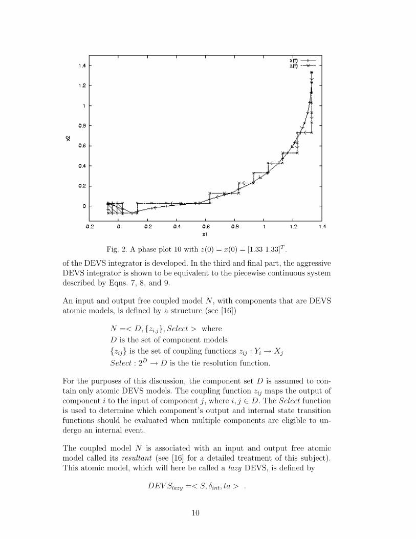
Fig. 2. A phase plot 10 with z(0) = x(0) = [1.33 1.33]T .
of the DEVS integrator is developed. In the third and final part, the aggressiveDEVS integrator is shown to be equivalent to the piecewise continuous systemdescribed by Eqns. 7, 8, and 9.
An input and output free coupled model N , with components that are DEVSatomic models, is defined by a structure (see [16])
N =< D, {zi,j}, Select > where
D is the set of component models
{zij} is the set of coupling functions zij : Yi → Xj
Select : 2D → D is the tie resolution function.
For the purposes of this discussion, the component set D is assumed to con-tain only atomic DEVS models. The coupling function zij maps the output ofcomponent i to the input of component j, where i, j ∈ D. The Select functionis used to determine which component’s output and internal state transitionfunctions should be evaluated when multiple components are eligible to un-dergo an internal event.
The coupled model N is associated with an input and output free atomicmodel called its resultant (see [16] for a detailed treatment of this subject).This atomic model, which will here be called a lazy DEVS, is defined by
DEV Slazy =< S, δint, ta > .
10
The state set S isS =
∏
d∈D
Qd
where Qd is the set of total states (sd, ed) of the atomic model d. The timeadvance function of the resultant is
ta(s) = min{σd | d ∈ D} (11)
where for each component d, σd = tad(sd)−ed. That is, σd is the time remaininguntil the next internal event of component d.
The imminent set of the coupled model N that corresponds to the state s ofthe resultant is given by IMM(s) = {d | d ∈ D & σd = ta(s)}. This describesthe set of components that have minimum remaining time σd (i.e., they arecandidates to undergo an internal event).
The internal transition function of the resultant is defined in the followingway. Let s = (..., (sd, ed), ...) and d∗ = Select(IMM(s)). Then
δint(s) = s′ = (..., (s′d, e′d), ...) , where
(s′d, e′d) =
(δint,d(sd), 0) if d = d∗
(δext,d(sd, ed + ta(s), xd), 0) if xd 6= ∅
(sd, ed + ta(s)) if xd = ∅
where xd = zd∗,d(λd∗(sd∗)) .
When the function δint,d is evaluated, it is said that an internal event hasoccurred at component d. Evaluation of δext,d is called an external event, andthe xd = ∅ case is called a non-event. The derivation of the resultant can befound in [16].
An aggressive DEVS can be specified over the same set of components as a lazyDEVS. The aggressive DEVS time advance function and state set are identicalto those of the lazy DEVS. The internal transition function is defined in termsof a set of functions δ∅,d : Qd × R → Qd and δx,d : Qd × Xd → Qd. There is oneδ∅,d function and one δx,d function for each component. The aggressive DEVSinternal transition function is given by
(..., (s′d, e′d), ...) = δint((..., (sd, ed), ...)) , where
(s′d, e′d) =
(δint,d(sd), 0) if d = d∗
δx,d(δ∅,d((sd, ed), ta(s)), xd) if xd 6= ∅
δ∅,d((sd, ed), ta(s)) if xd = ∅
where xd = zd∗,d(λd∗(sd∗)) .
The initial state of the aggressive and lazy DEVS are constrained to be iden-
11
tical with all ed = 0. The δ∅,d and δx,d functions are constrained such that thefollowing properties hold;
(1) Autonomous behavior is preserved, i.e.,
(s′d, e′d) = δ∅,d((sd, 0), ed) ⇒ δint,d(s
′d) = δint,d(sd) & λd(s
′d) = λd(sd)
(2) The external transition function is preserved, i.e.,
δx,d(δ∅,d((sd, ed), t), x) = (δext,d(sd, ed + t, x), 0)
(3) The time advance function is preserved, i.e.,
(s′d, e′d) = δ∅,d((sd, ed), t) ⇒ tad(s
′d) − e′d = tad(sd) − (ed + t)
(4) δ∅,d has the composition property
δ∅,d((sd, ed), α + β) = δ∅,d(δ∅,d((sd, ed), α), β)
If all of these properties are satisfied, then the following is true.
Theorem 4. Let s(t) denote the state trajectory of the lazy DEVS and s(t)the state trajectory of the aggressive DEVS. Let t∗ denote any time at which
some component model of the lazy DEVS undergoes an internal or external
event. Let sd(t) denote the trajectory of that component as it evolves as part of
the lazy DEVS, and sd(t) the corresponding component trajectory as it appears
as part of the aggressive DEVS. Then
sd(0) = sd(0) and
sd(t∗) = sd(t
∗)
Proof. The proof is accomplished by induction on the number of internal andexternal events that occur in the execution of the lazy DEVS.
BASE CASE: The statement sd(0) = sd(0) follows directly from the asser-tion that s(0) = s(0). Let t1 denote the first event occurring in the lazy DEVS.So t1 = ta(s(0)) = ta(s(0)). Hence, the first event time of the aggressive andlazy DEVS coincide.
Let d be a component that undergoes an internal or external event. If it is aninternal event, then ta(s) = tad(sd) and both the aggressive and lazy DEVSupdate sd using δint,d. If it is an external event, then it follows from property2 that δx,d(δ∅,d((sd, 0), ta(s)), x) = (δext,d(sd, ta(s), x), 0). So sd(t1) = sd(t1).
INDUCTIVE STEP: Assume that the theorem holds for every subsequentlazy DEVS event time t2, t3, ..., tn and consider the next event at time tn+1.
12
Let d be a component undergoing an internal or external event at time tn+1
as part of the lazy DEVS evolution. Let the total state of this component attime tn be (sd, ed). From the induction hypothesis, sd(tn − ed) = sd(tn − ed).That is, they agree on the state of component d when it last changed as partof the lazy DEVS evolution. Using this fact and the composition property ofδ∅,d, the corresponding total state of the aggressive DEVS component at timetn can be written as (s′d, e
′d) = δ∅,d((sd, 0), ed).
Suppose that component d is selected by the lazy DEVS to undergo an internalevent at time tn+1. So
tn+1 = tn + tad(sd) − ed .
It follows from property 3 that the corresponding next event time of the ag-gressive DEVS component is
tn + tad(s′d) − e′d
= tn + tad(sd) − (0 + ed)
= tn + tad(sd) − ed
= tn+1 ,
and so it too will undergo an internal event at time tn+1. More over, it followsfrom property 1 that
δint,d(sd) = δint,d(s′d) , so
sd(tn+1) = sd(tn+1) .
Notice that tn+1 defines the next event time of both the aggressive and lazyDEVS. Also, the induction hypothesis requires that tn be the previous eventtime for both DEVS. Consequently, ta(s(tn)) = ta(s(tn)), or to be brief,ta(s) = ta(s) at all event times. If d undergoes an external event, then itfollows from this fact, property 1, property 4, and property 2 that
xd = zd∗,d(λd∗(sd∗)) = zd∗,d(λd∗(s′d∗)) and
(δext,d(sd, ed + ta(s), xd), 0) = δx,d(δ∅,d((sd, 0), ed + ta(s)), xd)
where d∗ refers to the component that was selected for an internal event. It waspreviously shown that (s′d∗, e
′d∗) = δ∅,d∗((sd∗, 0), ed∗). Therefore, sd(tn+1) = sd(tn+1)
in this case as well.
The lazy DEVS integrator defined by system 6 can be written as an equivalentaggressive DEVS. To define this aggressive DEVS integrator, let
δ∅(((q, q, ql), e), τ) = ((q + (e + τ) · q, q, ql), 0) and
δx(((q, q, ql), e), x) = ((q, x, ql), 0) .
13
Properties 1 through 4 can be verified as follows;
(1) Preservation of autonomous behavior
δ∅(((q, q, ql), 0), e) = ((q + e · q, q, ql), 0) ⇒
δint((q, q, ql)) = (ql + ∆q · sgn(q), q, ql + ∆q · sgn(q)) = δint((q + e · q, q, ql))
& λ((q, q, ql)) = ql + ∆q · sgn(q) = λ((q + e · q, q, ql)) .
(2) Preservation of the external transition function
δx(δ∅(((q, q, ql), e), t), x) = δx(((q + (e + t) · q, q, ql), 0), x) =
((q + (e + t) · q, x, ql), 0) = (δext((q, q, ql), e + t, x), 0) .
(3) Preservation of the time advance function
δ∅(((q, q, ql), e), t) = ((q + (e + t) · q, q, ql), 0) ⇒
ta((q, q, ql)) − (e + t)
=ql ± ∆q − q
q− (e + t)
=ql ± ∆q − q
q−
(e + t) · q
q
=ql ± ∆q − q − (e + t) · q
q
=ql ± ∆q − (q + (e + t) · q)
q
= ta((q + (e + t) · q, q, ql)) .
(4) Composition property for δ∅
δ∅(δ∅(((q, q, ql), e), α), β)
= δ∅(((q + (α + e) · q, q, ql), 0), β)
= ((q + (α + e + β) · q, q, ql), 0)
= δ∅(((q, q, ql), e), α + β) .
The aggressive and lazy DEVS integrator networks have components whosestate trajectories agree at their lazy DEVS event times. A similar relationshipcan be established between the aggressive DEVS integrator network and thesystem described by Eqns. 7, 8, and 9.
Theorem 5. Consider the resultant of a network of aggressive DEVS integra-
tors. The integrators are coupled through a set of memory-less functions that
correspond to the rows of Az in Eqn. 7. Let the function fd(·) denote the dth
row of Az. Let t∗ denote an event time for the aggressive DEVS network, i.e.,
a time at which the aggressive DEVS internal transition function is evaluated.
Let the state trajectory of component d be denoted by qd(t), qd(t), and ql,d(t).
14
Then
qd(t∗) = xd(t
∗)
ql,d(t∗) = zd(t
∗) , and
qd(t∗) = fd(z(t∗)) = xd(t
∗) .
Proof. The theorem can always be made to hold at t = 0 by setting qd(0) =xd(0) = zd(0) = ql,d(0). Suppose the theorem holds at some time t∗, andconsider the event at the next event time t∗ + ta(s).
Let component d undergo an internal event at this time. The definition of theaggressive DEVS requires that ed = 0, and so
ta(s) = tad(sd) =
(ql,d + ∆q − qd)/q if q > 0
(ql,d − ∆q − qd)/q if q < 0
∞ otherwise
.
Without loss of generality, consider the case where q > 0. In this case
qd(t∗ + ta(s))
= ql,d(t∗) + ∆q
= qd(t∗) +
ql,d(t∗) + ∆q − qd(t
∗)
q(t∗)· qd(t
∗)
= qd(t∗) +
t∗+ta(s)∫
t∗
qd(t∗) dτ . (12)
From the induction hypothesis, qd(t∗) = xd(t
∗), ql,d(t∗) = zd(t
∗), and qd(t∗) =
xd(t∗). Moreover, xd(t) is constant until the next discrete change in z(t), and
so this time can be computed as
∆q + zd(t∗) − x(t∗)
x(t∗)= ta(s) .
By making the appropriate substitutions into Eqn. 12, it can be verified thatxd(t
∗+ta(s)) = qd(t∗+ta(s)). It follows immediately from this fact, Eqn. 8, and
Eqn. 9 that qd(t∗ + ta(s)) = xd(t
∗ + ta(s)) and ql,d(t∗ + ta(s)) = zd(t
∗ + ta(s)).
If d undergoes an external event at time t∗ + ta(s), then ql,d and zd remainunchanged, and consequently ql,d(t
∗ + ta(s)) = zd(t∗ + ta(s)). It is also true
15
that
xd(t∗ + ta(s)) = xd(t
∗) +
t∗+ta(s)∫
t∗
xd(t∗) dτ
= xd(t∗) + ta(s) · xd(t
∗) = qd(t∗) + ta(s) · xd(t
∗)
and so xd(t∗+ta(s)) = qd(t
∗+ta(s)). Moreover, the agreement of the imminentmodel state with the piecewise continuous system and property 1 ensures thatqd(t
∗ + ta(s)) = fd(z(t∗ + ta(s))) = xd(t∗ + ta(s)).
5 Discrete Time Linear Model of the DEVS Integrator
The system described by Eqns. 7, 8, and 9 can be rewritten as a time-varyinglinear system with bounded input. This is intuitively clear upon observing thatthe continuous formulation describes a sequence of line segments. Moreover,the time interval separating two different segments can be readily determinedfrom Eqn. 9 and the component-wise slope Az(t) of the line segment.
These observations can be formalized in the following way. Let ∆t(n) be thetime separating any two sequential discrete values of z (e.g., two adjacentpoints on the z(t) curves in Fig. 1 and 2). To be precise, let tn and tn+1 denotethe times at which these sequential values occur. Then ∆t(n) = tn+1 − tn.
The function z(t) is, by construction, constant in the interval [tn, tn+1). Thebehavior of x(t) in this interval can be determined directly from Eqn. 7 to be
x(tn+1) = x(tn) +
tn+1∫
tn
Az(tn) dt
= x(tn) + Az(tn)
tn+1∫
tn
dt
= x(tn) + (tn+1 − tn)Az(tn)
= x(tn) + ∆t(n)Az(tn) . (13)
Letting z(tn) = x(tn) + k(tn), Eqn. 13 can be rewritten as
x(tn+1) = x(tn) + ∆t(n)Ax(tn) + ∆t(n)Ak(tn)
= (I + ∆t(n)A)x(tn) + ∆t(n)Ak(tn) . (14)
Equation 9 requires that ‖k(tn)‖∞ ≤ ∆q, and so this is a time-varying linearsystem with bounded input. This formulation of the system is illustrated inFig. 3.
16
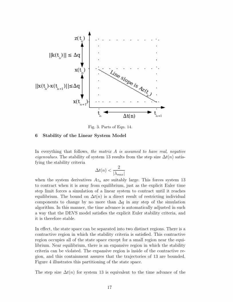
Fig. 3. Parts of Eqn. 14.
6 Stability of the Linear System Model
In everything that follows, the matrix A is assumed to have real, negative
eigenvalues. The stability of system 13 results from the step size ∆t(n) satis-fying the stability criteria
∆t(n) <2
|λmax|
when the system derivatives Azn are suitably large. This forces system 13to contract when it is away from equilibrium, just as the explicit Euler timestep limit forces a simulation of a linear system to contract until it reachesequilibrium. The bound on ∆t(n) is a direct result of restricting individualcomponents to change by no more than ∆q in any step of the simulationalgorithm. In this manner, the time advance is automatically adjusted in sucha way that the DEVS model satisfies the explicit Euler stability criteria, andit is therefore stable.
In effect, the state space can be separated into two distinct regions. There is acontractive region in which the stability criteria is satisfied. This contractiveregion occupies all of the state space except for a small region near the equi-librium. Near equilibrium, there is an expansive region in which the stabilitycriteria can be violated. The expansive region is inside of the contractive re-gion, and this containment assures that the trajectories of 13 are bounded.Figure 4 illustrates this partitioning of the state space.
The step size ∆t(n) for system 13 is equivalent to the time advance of the
17
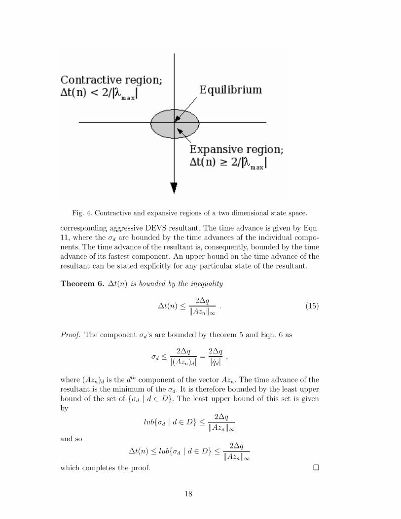
Fig. 4. Contractive and expansive regions of a two dimensional state space.
corresponding aggressive DEVS resultant. The time advance is given by Eqn.11, where the σd are bounded by the time advances of the individual compo-nents. The time advance of the resultant is, consequently, bounded by the timeadvance of its fastest component. An upper bound on the time advance of theresultant can be stated explicitly for any particular state of the resultant.
Theorem 6. ∆t(n) is bounded by the inequality
∆t(n) ≤2∆q
‖Azn‖∞. (15)
Proof. The component σd’s are bounded by theorem 5 and Eqn. 6 as
σd ≤2∆q
|(Azn)d|=
2∆q
|qd|,
where (Azn)d is the dth component of the vector Azn. The time advance of theresultant is the minimum of the σd. It is therefore bounded by the least upperbound of the set of {σd | d ∈ D}. The least upper bound of this set is givenby
lub{σd | d ∈ D} ≤2∆q
‖Azn‖∞
and so
∆t(n) ≤ lub{σd | d ∈ D} ≤2∆q
‖Azn‖∞
which completes the proof.
18

This bound on the time advance of the resultant forces the eigenvalues ofI + ∆t(n)A to have magnitudes less than 1 when the system is sufficientlyfar from its equilibrium. More specifically, if the system is a suitable distancefrom equilibrium, then ∆t(n) satisfies
∆t(n) <2
|λmax|
where |λmax| is the largest magnitude of the eigenvalues belonging to A.
Theorem 7. If
‖Az(tn)‖∞ > ∆q|λmax|
then
∆t(n) <2
|λmax|.
Proof. Let
‖Az(tn)‖∞ > ∆q|λmax| .
Inequality 15 can be rearranged to show that
2∆q
∆t(n)≥ ‖Azn‖∞ .
Therefore2∆q
∆t(n)> ∆q|λmax|
and it follows that
∆t(n) <2
|λmax|.
The link between explicit Euler stability (see, e.g., [19], or any introductorynumerical analysis textbook) and the stability of the DEVS integrator networkcan be stated explicitly as a corollary to theorem 7.
Corollary 8. Let hlimit be the maximum time step in a stable, explicit Euler
simulation of a stable linear system. If ‖Azn‖∞ > ∆q|λmax|, then ∆t(n) <hlimit.
It follows theorem 7 that Eqn. 14 has ultimately bounded trajectories.
Theorem 9. Consider the system described by Eqn. 14. For all n
∆t(n) <2
|λmax|,
19
then
‖x(tn)‖∞ <2∆qβ
|λmax|‖A‖∞
as n → ∞. The constant 0 < β < ∞ is specific to the system under consider-
ation.
Proof. Let φ(tn, tm) = (I + ∆t(n − 1)A)(I + ∆t(n − 2)A)...(I + ∆t(m)A), or,more concisely
φ(tn, tm) =n−m∏
p=1
(I + ∆t(n − p)A) .
It is well known from the theory of linear systems (see, e.g., [14]) that
x(tn) = φ(tn, 0)x(0) +n−1∑
q=0
(
φ(tn, tq+1)∆t(q)Ak(tq)
)
.
It follows from the hypothesis and well known properties of the infinity-normthat
‖x(tn)‖∞ ≤ ‖φ(tn, 0)x(0)‖∞ +n−1∑
q=0
(
‖φ(tn, tq+1)∆t(q)Ak(tq)‖∞
)
≤ ‖φ(tn, 0)x(0)‖∞ +n−1∑
q=0
(
‖φ(tn, tq+1)‖∞ · |∆t(q)| · ‖A‖∞ · ‖k(tq)‖∞
)
< ‖φ(tn, 0)x(0)‖∞ +2∆q
|λmax|‖A‖∞
n−1∑
q=0
‖φ(tn, tq+1)‖∞ .
The upper bound on ∆t(n) constrains the eigenvalues of I + ∆t(n)A to havemagnitudes less than 1. Consequently, as n → ∞, ‖φ(tn, 0)x(0)‖∞ vanishesand
n−1∑
q=0
‖φ(tn, tq+1)‖∞ < ∞ .
Moreover,‖φ(tn, tk)‖∞‖φ(tn, tk−1)‖∞
< 1
and so, by the ratio test, the sum converges as n → ∞. Let β be this limit tocomplete the proof.
Theorem 9 shows that x(t) is ultimately contained in a bounded region, pro-vided that ‖Az(tn)‖∞ is sufficiently large, or, more specifically, if it satisfiestheorem 7. It remains to show that violations of theorem 7 can not persist.That is, if a system enters the expansive region, then it must remain in thatregion (e.g., if z(t) = 0) or once again enter the contractive region.
20
Suppose that, for some tm, the hypothesis of theorem 9, and consequentlytheorem 7, fails to hold. That is, for some time tm,
‖Az(tm)‖∞ ≤ ∆q|λmax| . (16)
If inequality 16 is satisfied at all times subsequent to tm (e.g., if z(tm) = 0)then 16 describes a bound on x(t) that is proportional to ∆q. More specifically,∀n > m , x(tn) must satisfy
‖A(x(tn) + k(tn))‖∞ ≤ ∆q|λmax| ,
where Eqn. 9 constrains k(tn) such that ‖k(tn)‖∞ ≤ ∆q.
Otherwise, for some n > m, the hypothesis of theorem 9 holds. In this case,x(tn) is bounded by the region described in theorem 9 or the smallest valueof ‖x(t)‖∞ for which theorem 7 holds. More specifically, there is a constantK > 1 such that
‖A(x(tn) + k(tn))‖∞ ≤ K∆q|λmax| .
In either case, ‖x(tn)‖∞ is ultimately contained in a region whose dimensionsare proportional to ∆q. The conclusion of this argument is restated as theorem10.
Theorem 10. Consider the system described by Eqn. 14. As tn → ∞, x(tn)must satisfy
‖A(x(tn) + k(tn))‖∞ ≤ K∆q|λmax|
where K > 1, or
‖x(tn)‖∞ <2∆qβ
|λmax|‖A‖∞
where 0 < β < ∞ is a constant specific to the system under consideration.
Theorem 7 defines the outer edge of the expansive region, and 9 gives a conser-vative estimate of the inner edge of the contractive region. Theorem 10 statesthat the system must ultimately be trapped within one of these bounds. Inparticular, the system becomes trapped within the expansive region if it hap-pens the reach equilibrium. Otherwise, the system will wander in an areacontained within the conservative bound on the inner edge of the contractiveregion.
7 Comparing QSS and Forward Euler
A synchronous form of the first order discrete event method can be constructedby updating every state variable simultaneously. This derived method uses an
21
adaptive time step that is chosen so that the fastest component changes itsmagnitude by ∆q. 2
This method simulates a set of ordinary differential equations in the form
x = f(x)
with a recursive function
xn+1 = xn + h(n)f(xn) , where
h(n) =∆q
‖f(xn)‖∞. (17)
The method stops if ‖f(xn)‖∞ = 0 (i.e., if an equilibrium is reached).
When simulating a linear system x = Ax, Eqn. 17 becomes
xn+1 = xn +∆q
‖Axn‖∞xn =
(
I +∆q
‖Axn‖∞
)
xn .
This system is the same as system 13 with kn = 0. The step size at the nthstep is
h(n) =∆q
‖Axn‖∞where 13 has a step size
∆t(n) <2∆q
‖Azn‖∞.
Within trajectory segments that are monotonically increasing or decreasing,∆t(n) will, in fact, be bounded by ∆q‖Azn‖∞. The 2∆q term applies onlywhen hysteresis can cause the system to move a distance further than ∆qbetween events (see [1]).
The numerical properties of the synchronous DEVS integrator are similar tothose of the asynchronous form. The synchronous integrator will, in general,require fewer simulation cycles (i.e., fewer state changes of the resultant) tocover an interval of time. However, it will update every component at eachsimulation cycle. Consequently, the total number of component updates couldbe (very) large when compared with the asynchronous scheme, even if theasynchronous scheme requires more simulation cycles. The synchronous inte-grator will also create smaller errors than the asynchronous form because itforces the slower components to update at state space intervals smaller than∆q.
2 The synchronous DEVS model ensures that every component sees the most re-cently computed state values for its neighbors. This is unlike the aggressive DEVSmodel in which components only see new neighbor values when the neighbors qvariable reaches a threshold crossing (i.e., |q − ql| = ∆q).
22
The asynchronous form trades error for, potentially, reduced execution time. Ifindividual components are loosely coupled 3 and their rates vary widely, thenthe asynchronous form could require significantly fewer component updatesthan the synchronous form. The additional errors in the asynchronous methodresult from evaluating slower components less often than would be done usingthe synchronous method.
The synchronous integrator is useful for comparing the relative properties ofdiscrete event and other fixed and adaptive time stepping methods. It closelymimics the error and stability properties of the asynchronous model. If thesynchronous model has error, stability, and/or performance properties thatlook attractive relative to other methods, then the asynchronous model couldprovide an additional performance boost via its locally adaptive time advance.Similarly, if the synchronous model looks unattractive for some particularproblem, then the extra performance obtained with the asynchronous methodwill need to be very significant for it to be considered a viable alternative.
Equation 17 is an adaptive form of the explicit Euler method
xn+1 = xn + hf(xn) . (18)
If h is fixed to be the smallest h(n) observed over a simulation interval (e.g.,as is done in [5]), then Eqn. 18 will require a larger number of steps thanboth the synchronous and asynchronous DEVS methods. However, Eqn. 18will use smaller time steps to evaluate slower dynamics, thereby giving itbetter accuracy than either adaptive method. If h is fixed to be the largesth(n) < 2/|λmax|, then Eqn. 18 will need fewer steps than the adaptive methodsbut will, in general, exhibit larger errors.
The errors exhibited by the asynchronous method will, in general, be largerthan those of the synchronous method. However, for systems with looselycoupled components and a large range of rates, the asynchronous methodmay perform better by reducing the total number of component updates.
These observations, applied to linear systems, are summarized in Table 1.Where the time advance of the DEVS schemes is limited by theorem 7, theexplicit Euler method can be used to bound the errors that will be observed ina first order discrete event simulation of a linear system. The largest explicitEuler error that occurs when using a time step min {h(n)} gives a lowerbound on the maximum error that will be observed in the discrete eventsimulation. The largest explicit Euler error that occurs when using a time
3 By loosely coupled we mean that the number of integrator inputs influenced byan integrator output is small relative to the dimension of the network. In linearsystems, this is caused by a sparse transition matrix. An example will be given inSection 8.
23
step max {h(n) | h(n) < 2/|λmax|} gives an upper bound on the maximumerror that will be observed in the discrete event simulation.
Table 1Relative errors of synchronous and asynchronous DEVS methods with respect toexplicit Euler
Euler time step Relation to maximum DEVS error
min {h(n)} maximum Euler error < maximum DEVS error
max {h(n) | h(n) < 2/|λmax|} maximum Euler error > maximum DEVS error
8 Examples
The examples in this section demonstrate the error and stability propertiesdeveloped in the previous sections. It also highlights the computational ad-vantage of the first order QSS scheme, relative to the other first order methodsdescribed in Sect. 7, for simulating large, loosely coupled systems. Specifically,the first order QSS method generates errors comparable to other first order ac-curate methods while realizing a substantial reduction in computational costsfor large, loosely coupled systems. We anticipate that this advantage will carryover to higher order QSS schemes (see, e.g., [2, 20–22]).
Consider the system x = −αx, where α > 0. This system has a single statevariable. The synchronous and asynchronous DEVS methods are identical fora system with a single variable. A (synchronous or asynchronous) discreteevent simulation of this system is described exactly by
xn+1 = xn − h(n)αxn , where
h(n) =∆q
|αxn|.
Whenever |xn| ≥ ∆q/2, then h(n) ≤ 2/α. Noting that α is the eigenvalue ofthis system, we see that a discrete event simulation of this system is stableregardless of the choice of ∆q. The first order quantization method automat-ically adjusts its time step to maintain stability.
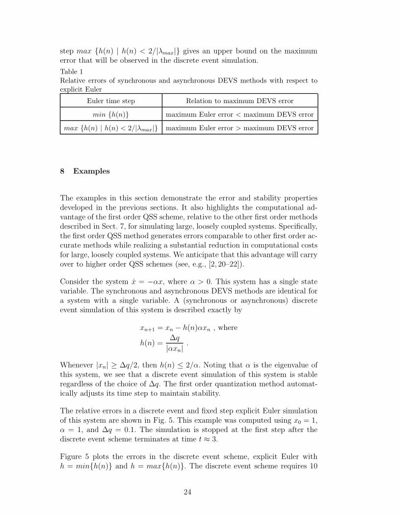
The relative errors in a discrete event and fixed step explicit Euler simulationof this system are shown in Fig. 5. This example was computed using x0 = 1,α = 1, and ∆q = 0.1. The simulation is stopped at the first step after thediscrete event scheme terminates at time t ≈ 3.
Figure 5 plots the errors in the discrete event scheme, explicit Euler withh = min{h(n)} and h = max{h(n)}. The discrete event scheme requires 10
24
steps to complete the simulation; with h = min{h(n)} = 0.1, explicit Eulerrequires 30 steps; with h = max{h(n)} = 1, explicit Euler requires 3 steps.
0
0.05
0.1
0.15
0.2
0.25
0.3
0.35
0.4
0 0.5 1 1.5 2 2.5 3
erro
r
time
DEVSh=min{h(n)}
h=max{h(n)}
Fig. 5. Comparison of errors produced by DEVS and explicit Euler when simulatingx = −x.
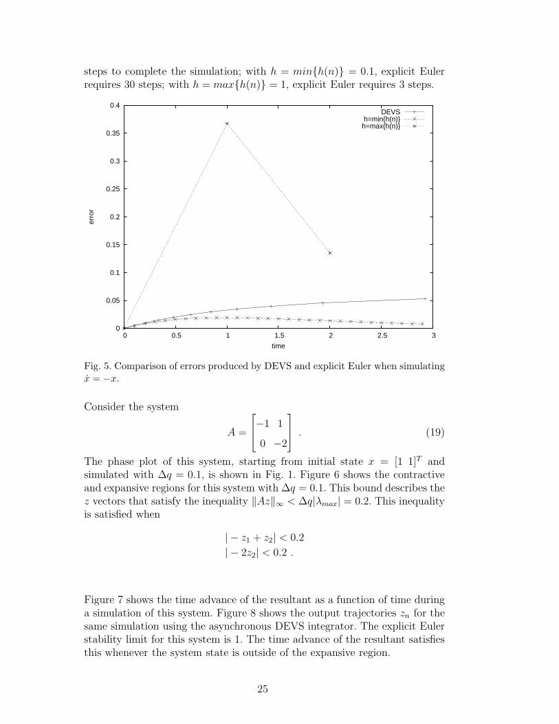
Consider the system
A =
−1 1
0 −2
. (19)
The phase plot of this system, starting from initial state x = [1 1]T andsimulated with ∆q = 0.1, is shown in Fig. 1. Figure 6 shows the contractiveand expansive regions for this system with ∆q = 0.1. This bound describes thez vectors that satisfy the inequality ‖Az‖∞ < ∆q|λmax| = 0.2. This inequalityis satisfied when
| − z1 + z2| < 0.2
| − 2z2| < 0.2 .
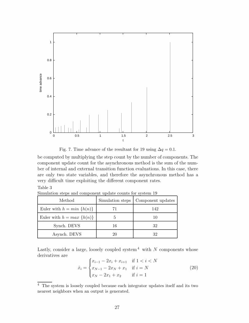
Figure 7 shows the time advance of the resultant as a function of time duringa simulation of this system. Figure 8 shows the output trajectories zn for thesame simulation using the asynchronous DEVS integrator. The explicit Eulerstability limit for this system is 1. The time advance of the resultant satisfiesthis whenever the system state is outside of the expansive region.
25
-0.2
-0.15
-0.1
-0.05
0
0.05
0.1
0.15
0.2
-0.4 -0.3 -0.2 -0.1 0 0.1 0.2 0.3 0.4
z2
z1
Bound of the expansive region
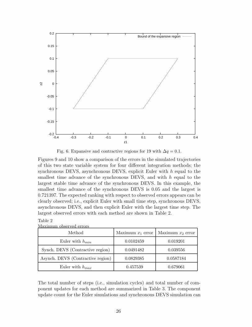
Fig. 6. Expansive and contractive regions for 19 with ∆q = 0.1.
Figures 9 and 10 show a comparison of the errors in the simulated trajectoriesof this two state variable system for four different integration methods; thesynchronous DEVS, asynchronous DEVS, explicit Euler with h equal to thesmallest time advance of the synchronous DEVS, and with h equal to thelargest stable time advance of the synchronous DEVS. In this example, thesmallest time advance of the synchronous DEVS is 0.05 and the largest is0.721397. The expected ranking with respect to observed errors appears can beclearly observed; i.e., explicit Euler with small time step, synchronous DEVS,asynchronous DEVS, and then explicit Euler with the largest time step. Thelargest observed errors with each method are shown in Table 2.
Table 2Maximum observed errors
Method Maximum x1 error Maximum x2 error
Euler with hmin 0.0102459 0.019201
Synch. DEVS (Contractive region) 0.0491482 0.039556
Asynch. DEVS (Contractive region) 0.0829385 0.0587184
Euler with hmax 0.457539 0.679061
The total number of steps (i.e., simulation cycles) and total number of com-ponent updates for each method are summarized in Table 3. The componentupdate count for the Euler simulations and synchronous DEVS simulation can
26
0
0.2
0.4
0.6
0.8
1
0 0.5 1 1.5 2 2.5 3
time
adva
nce
t
Fig. 7. Time advance of the resultant for 19 using ∆q = 0.1.
be computed by multiplying the step count by the number of components. Thecomponent update count for the asynchronous method is the sum of the num-ber of internal and external transition function evaluations. In this case, thereare only two state variables, and therefore the asynchronous method has avery difficult time exploiting the different component rates.
Table 3Simulation steps and component update counts for system 19
Method Simulation steps Component updates
Euler with h = min {h(n)} 71 142
Euler with h = max {h(n)} 5 10
Synch. DEVS 16 32
Asynch. DEVS 20 32
Lastly, consider a large, loosely coupled system 4 with N components whosederivatives are
xi =
xi−1 − 2xi + xi+1 if 1 < i < N
xN−1 − 2xN + x1 if i = N
xN − 2x1 + x2 if i = 1
(20)
4 The system is loosely coupled because each integrator updates itself and its twonearest neighbors when an output is generated.
27
0
0.1
0.2
0.3
0.4
0.5
0.6
0.7
0.8
0.9
1
0 0.5 1 1.5 2 2.5 3 3.5 4
x
t
x1x2
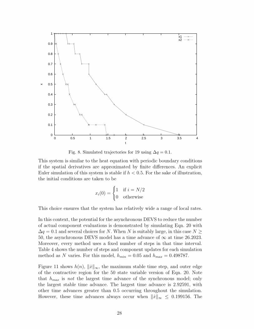
Fig. 8. Simulated trajectories for 19 using ∆q = 0.1.
This system is similar to the heat equation with periodic boundary conditionsif the spatial derivatives are approximated by finite differences. An explicitEuler simulation of this system is stable if h < 0.5. For the sake of illustration,the initial conditions are taken to be
xi(0) =
1 if i = N/2
0 otherwise
This choice ensures that the system has relatively wide a range of local rates.
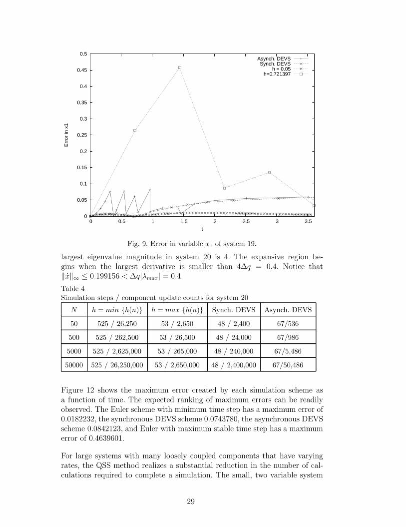
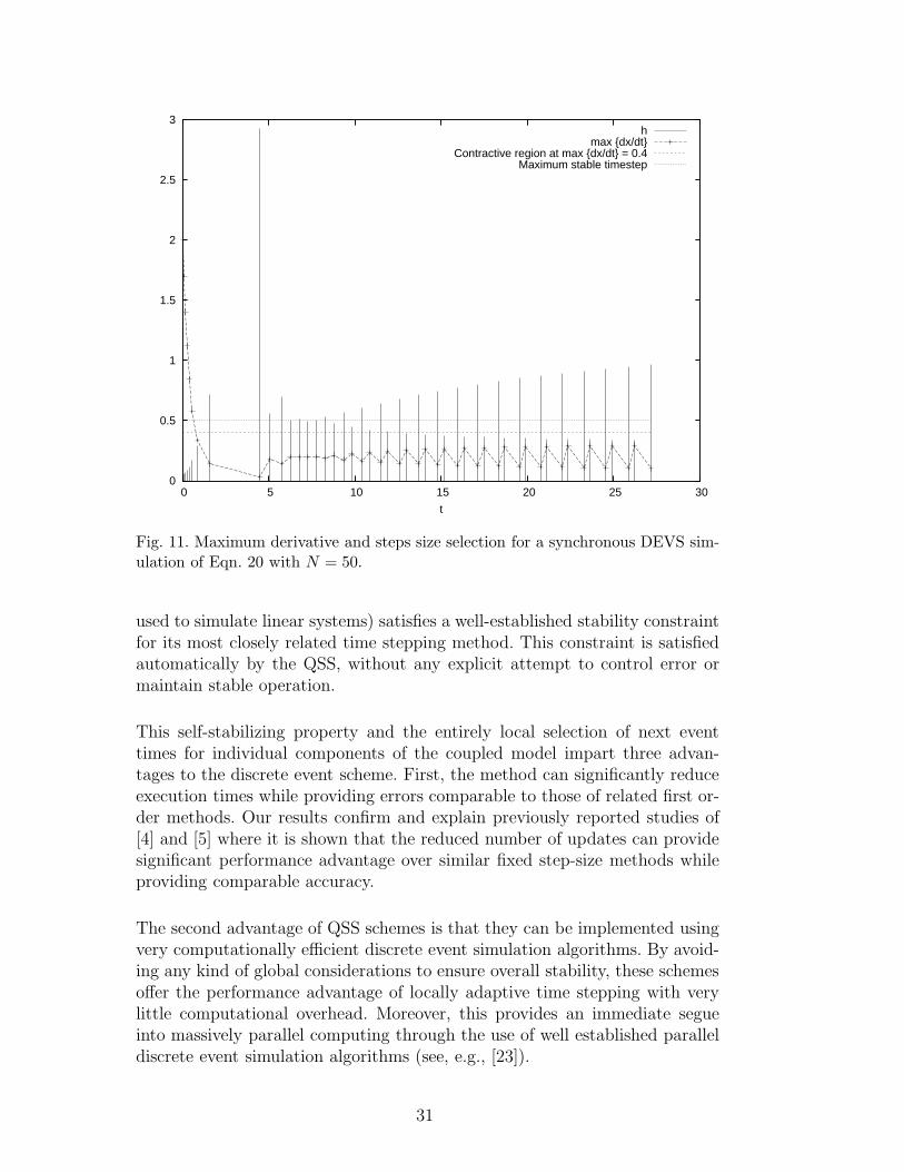
In this context, the potential for the asynchronous DEVS to reduce the numberof actual component evaluations is demonstrated by simulating Eqn. 20 with∆q = 0.1 and several choices for N . When N is suitably large, in this case N ≥50, the asynchronous DEVS model has a time advance of ∞ at time 26.2023.Moreover, every method uses a fixed number of steps in that time interval.Table 4 shows the number of steps and component updates for each simulationmethod as N varies. For this model, hmin = 0.05 and hmax = 0.498787.
Figure 11 shows h(n), ‖x‖∞, the maximum stable time step, and outer edgeof the contractive region for the 50 state variable version of Eqn. 20. Notethat hmax is not the largest time advance of the synchronous model; onlythe largest stable time advance. The largest time advance is 2.92591, withother time advances greater than 0.5 occurring throughout the simulation.However, these time advances always occur when ‖x‖∞ ≤ 0.199156. The
28
0
0.05
0.1
0.15
0.2
0.25
0.3
0.35
0.4
0.45
0.5
0 0.5 1 1.5 2 2.5 3 3.5
Err
or in
x1
t
Asynch. DEVSSynch. DEVS
h = 0.05h=0.721397
Fig. 9. Error in variable x1 of system 19.
largest eigenvalue magnitude in system 20 is 4. The expansive region be-gins when the largest derivative is smaller than 4∆q = 0.4. Notice that‖x‖∞ ≤ 0.199156 < ∆q|λmax| = 0.4.
Table 4Simulation steps / component update counts for system 20
N h = min {h(n)} h = max {h(n)} Synch. DEVS Asynch. DEVS
50 525 / 26,250 53 / 2,650 48 / 2,400 67/536
500 525 / 262,500 53 / 26,500 48 / 24,000 67/986
5000 525 / 2,625,000 53 / 265,000 48 / 240,000 67/5,486
50000 525 / 26,250,000 53 / 2,650,000 48 / 2,400,000 67/50,486
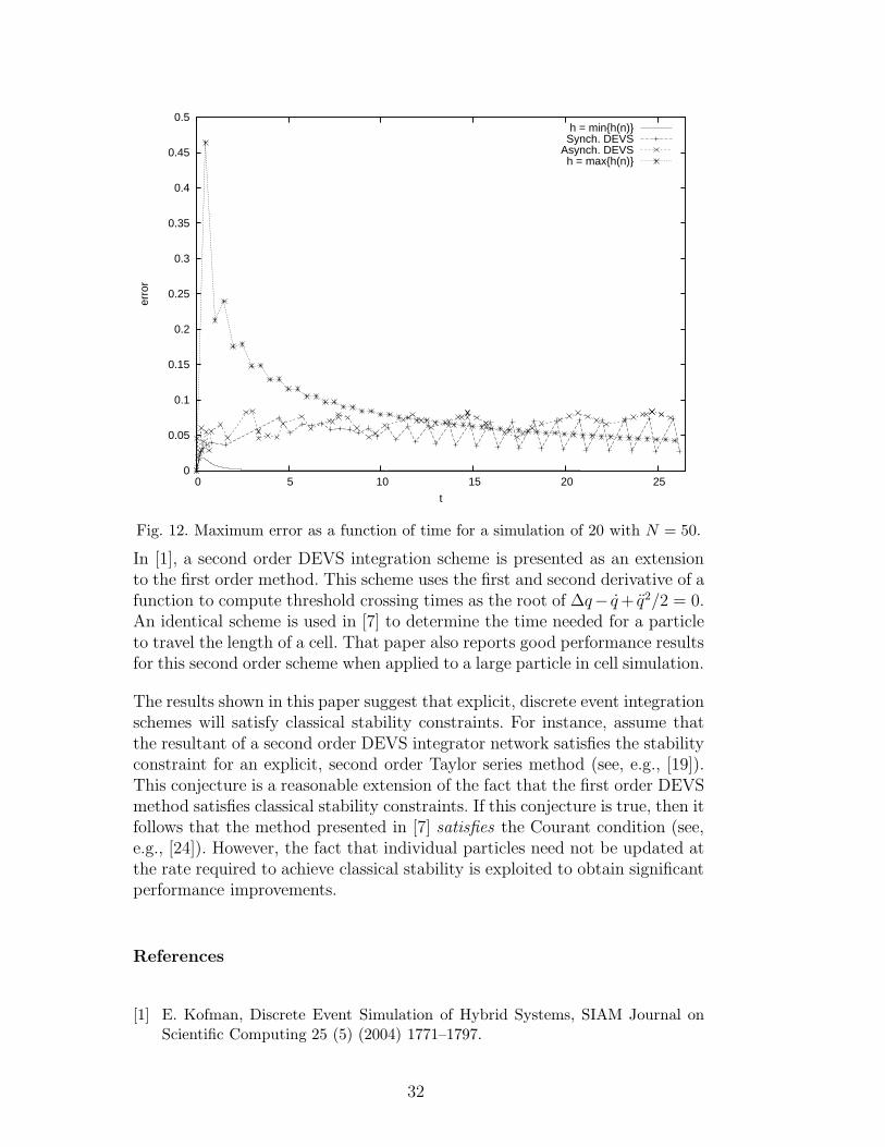
Figure 12 shows the maximum error created by each simulation scheme asa function of time. The expected ranking of maximum errors can be readilyobserved. The Euler scheme with minimum time step has a maximum error of0.0182232, the synchronous DEVS scheme 0.0743780, the asynchronous DEVSscheme 0.0842123, and Euler with maximum stable time step has a maximumerror of 0.4639601.
For large systems with many loosely coupled components that have varyingrates, the QSS method realizes a substantial reduction in the number of cal-culations required to complete a simulation. The small, two variable system
29
0
0.1
0.2
0.3
0.4
0.5
0.6
0.7
0 0.5 1 1.5 2 2.5 3 3.5
Err
or in
x2
t
Asynch. DEVSSynch. DEVS
h = 0.05h=0.721397
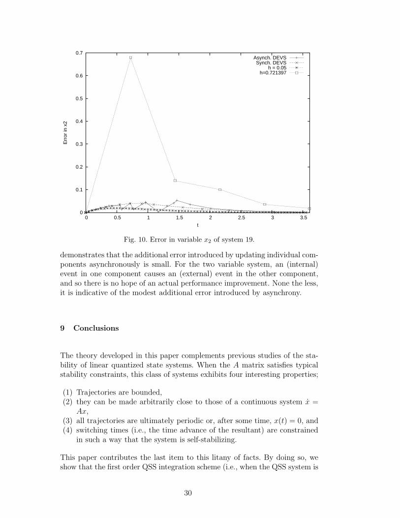
Fig. 10. Error in variable x2 of system 19.
demonstrates that the additional error introduced by updating individual com-ponents asynchronously is small. For the two variable system, an (internal)event in one component causes an (external) event in the other component,and so there is no hope of an actual performance improvement. None the less,it is indicative of the modest additional error introduced by asynchrony.
9 Conclusions
The theory developed in this paper complements previous studies of the sta-bility of linear quantized state systems. When the A matrix satisfies typicalstability constraints, this class of systems exhibits four interesting properties;
(1) Trajectories are bounded,(2) they can be made arbitrarily close to those of a continuous system x =
Ax,(3) all trajectories are ultimately periodic or, after some time, x(t) = 0, and(4) switching times (i.e., the time advance of the resultant) are constrained
in such a way that the system is self-stabilizing.
This paper contributes the last item to this litany of facts. By doing so, weshow that the first order QSS integration scheme (i.e., when the QSS system is
30
0
0.5
1
1.5
2
2.5
3
0 5 10 15 20 25 30
t
hmax {dx/dt}
Contractive region at max {dx/dt} = 0.4Maximum stable timestep
Fig. 11. Maximum derivative and steps size selection for a synchronous DEVS sim-ulation of Eqn. 20 with N = 50.
used to simulate linear systems) satisfies a well-established stability constraintfor its most closely related time stepping method. This constraint is satisfiedautomatically by the QSS, without any explicit attempt to control error ormaintain stable operation.
This self-stabilizing property and the entirely local selection of next eventtimes for individual components of the coupled model impart three advan-tages to the discrete event scheme. First, the method can significantly reduceexecution times while providing errors comparable to those of related first or-der methods. Our results confirm and explain previously reported studies of[4] and [5] where it is shown that the reduced number of updates can providesignificant performance advantage over similar fixed step-size methods whileproviding comparable accuracy.
The second advantage of QSS schemes is that they can be implemented usingvery computationally efficient discrete event simulation algorithms. By avoid-ing any kind of global considerations to ensure overall stability, these schemesoffer the performance advantage of locally adaptive time stepping with verylittle computational overhead. Moreover, this provides an immediate segueinto massively parallel computing through the use of well established paralleldiscrete event simulation algorithms (see, e.g., [23]).
31
0
0.05
0.1
0.15
0.2
0.25
0.3
0.35
0.4
0.45
0.5
0 5 10 15 20 25
erro
r
t
h = min{h(n)}Synch. DEVS
Asynch. DEVSh = max{h(n)}
Fig. 12. Maximum error as a function of time for a simulation of 20 with N = 50.
In [1], a second order DEVS integration scheme is presented as an extensionto the first order method. This scheme uses the first and second derivative of afunction to compute threshold crossing times as the root of ∆q− q + q2/2 = 0.An identical scheme is used in [7] to determine the time needed for a particleto travel the length of a cell. That paper also reports good performance resultsfor this second order scheme when applied to a large particle in cell simulation.
The results shown in this paper suggest that explicit, discrete event integrationschemes will satisfy classical stability constraints. For instance, assume thatthe resultant of a second order DEVS integrator network satisfies the stabilityconstraint for an explicit, second order Taylor series method (see, e.g., [19]).This conjecture is a reasonable extension of the fact that the first order DEVSmethod satisfies classical stability constraints. If this conjecture is true, then itfollows that the method presented in [7] satisfies the Courant condition (see,e.g., [24]). However, the fact that individual particles need not be updated atthe rate required to achieve classical stability is exploited to obtain significantperformance improvements.
References
[1] E. Kofman, Discrete Event Simulation of Hybrid Systems, SIAM Journal onScientific Computing 25 (5) (2004) 1771–1797.
32
[2] J. Nutaro, Constructing Multi-Point Discrete Event Integration Schemes, in:Proceedings of the 37th Winter Simulation Conference, Winter SimulationConference, 2005, pp. 267–273.
[3] B. P. Zeigler, H. Sarjoughian, H. Praehofer, Theory of Quantized Systems:DEVS Simulation of Perceiving Agents, Cybernetics and Systems 31 (6) (2000)611–647.
[4] A. Muzy, A. Aiello, P.-A. Santoni, B. P. Zeigler, J. J. Nutaro,R. Jammalamadaka, Discrete Event Simulation of Large-Scale SpatialContinuous Systems, in: Proceedings of the 2005 IEEE International Conferenceon Systems, Man and Cybernetics, Vol. 4, IEEE, Hawaii, USA, 2005, pp. 2991–2998.
[5] J. J. Nutaro, B. P. Zeigler, R. Jammalamadaka, S. R. Akerkar, Discrete EventSolution of Gas Dynamics within the DEVS Framework, in: P. M. A. Sloot,D. Abramson, A. V. Bogdanov, J. Dongarra, A. Y. Zomaya, Y. E. Gorbachev(Eds.), International Conference on Computational Science, Vol. 2660 of LectureNotes in Computer Science, Springer, Melbourne, Australia, 2003, pp. 319–328.
[6] G. A. Wainer, N. Giambiasi, Cell-DEVS/GDEVS for Complex ContinuousSystems, SIMULATION 81 (2) (2005) 137–151.
[7] H. Karimabadi, J. Driscoll, Y. Omelchenko, N. Omidi, A New AsynchronousMethodology for Modeling of Physical Systems: Breaking the Curse of CourantCondition, Journal of Computational Physics 205 (2) (2005) 755–775.
[8] Y. Tang, K. Perumalla, R. Fujimoto, H. Karimabadi, J. Driscoll,Y. Omelchenko, Optimistic Parallel Discrete Event Simulations of PhysicalSystems Using Reverse Computation, in: Proceedings of the 2005 Workshopon Principles of Advanced and Distributed Simulation (PADS 2005), 2005, pp.26–35.
[9] N. Lynch, R. Segala, F. Vaandrager, Hybrid I/O Automata, Information andComputation 185 (1) (2003) 105–157.
[10] A. S. Matveev, A. V. Savkin, Qualitative Theory of Hybrid Dynamical Systems,Birkhauser, Boston, 2000.
[11] A. Logg, Multi-Adaptive Galerkin Methods for ODEs I, SIAM Journal onScientific Computing 24 (6) (2002) 1879–1902.
[12] J. M. Esposito, V. Kumar, An Asynchronous Integration and Event DetectionAlgorithm for Simulating Multi-Agent Hybrid Systems, ACM Transactions onModeling and Computer Simulation 14 (4) (2004) 363–388.
[13] A. Lew, , J. Marsden, M. Ortiz, M. West, Asynchronous Variational Integrators,Archive for Rational Mechanics and Analysis 167 (2003) 85–146.
[14] F. Szidarovszky, A. T. Bahill, Linear Systems Theory, Second Edition, CRCPress LLC, Boca Raton, Florida, 1998.
33
[15] E. Kofman, Non-Conservative Ultimate Bound Estimation in LTI PerturbedSystems, Automatica 41 (10) (2005) 1835–1838.
[16] B. P. Zeigler, H. Praehofer, T. G. Kim, Theory of Modeling and Simulation,2nd Edition, Academic Press, San Diego, CA, 2000.
[17] E. Kofman, S. Junco, Quantized-State Systems: A DEVS Approach forContinuous System Simulation, Transactions of the Society for ComputerSimulation International 18 (3) (2001) 123–132.
[18] J. Zhang, K. H. Johansson, J. Lygeros, S. Sastry, Dynamical SystemsRevisited: Hybrid Systems with Zeno Executions, in: Proceedings of the ThirdInternational Workshop on Hybrid Systems: Computation and Control (HSCC2000), Springer-Verlag, London, UK, 2000, pp. 451–464.
[19] A. Ralston, P. Rabinowitz, A First Course in Numerical Analysis, SecondEdition, Dover Publications, Mineola, New York, 1978.
[20] E. Kofman, A Third Order Discrete Event Method for Continuous SystemSimulation. Part I: Theory, Tech. Rep. LSD0501, School of ElectronicEngineering, Universidad Nacional de Rosario, Rosario, Argentina (2005).
[21] E. Kofman, A Third Order Discrete Event Method for Continuous SystemSimulation. Part II: Applications, Tech. Rep. LSD0502, School of ElectronicEngineering, Universidad Nacional de Rosario, Rosario, Argentina (2005).
[22] E. Kofman, A Second-Order Approximation for DEVS Simulation ofContinuous Systems, SIMULATION 78 (2) (2002) 76–89.
[23] R. M. Fujimoto, Parallel and Distributed Simulation Systems, Wiley-Interscience, 1999.
[24] G. Strang, Introduction to Applied Mathematics, Wellsley-Cambridge Press,Wellesley, MA, 1986.
34