Embed Size (px)
Citation preview

The existence and stability of solitons in
discrete nonlinear Schrödinger equations
Mahdhivan Syafwan, S.Si.
Thesis submitted to The University of Nottingham
for the degree of Doctor of Philosophy
November 2012

“...Then which of the favours of your Lord would you deny?...”
(QS. Ar-Rahman 55)
Dedicated to:
My parents, my wife and my son.
i

Acknowledgements
First and above all, I praise the Almighty Allah, the Most Gracious and the Most Mer-
ciful. Indeed, it is only because of His favours and bounties that I got the ability to
accomplish this thesis.
There were many people who contributed in the completion of this thesis. Thus, I
take this opportunity to express my gratitude to them. However, to mention them all
here is indeed not possible, but they will never be forgotten. Firstly, and certainly, I
would like to offer my deepest gratitude to Dr. Hadi Susanto and Dr. Stephen M. Cox
who provided me invaluable supervision throughout my PhD studies. I feel honoured
while getting benefits from their knowledge and mathematical experiences. I am also
grateful for their kind support, guidance and suggestions during my studies, including
their useful comments and corrections on the manuscripts of this thesis. Special thanks
should be addressed to mas Hadi who helped me lot during my stay in the UK.
Next, I must express my sincere thanks and respect to my parents, Mama and Papa,
for their boundless love and unlimited support. Their continuous prayers brought me
at this stage. My sincere thanks also goes to my late grandmother (may Allah bless
her with jannah) for her amazing kindness and care, as well as to my father-in-law who
always treated me as his own son.
The most heartfelt gratitude is to my beloved wife and truly friend, Maya Sari Syahrul,
for her total moral support, passion and companionship. Also for my little prince and
beloved son, Faithulkhaliv Mahdhivan, the most lovely ‘gift’ who arrived in the period
of my studies. Both of you have been sources of my inspiration. Furthermore, I also
thanks to my brother and sister, Havid and Ivat, for their prayers and encouragement.
It is a pleasure to single out pak Saeed and Irfan bhai, for their help and warm brother-
hood. I also acknowledge Boris Malomed for his valuable suggestions while working
on variational approximations as well as Hill Meijer for fruitful discussions on Mat-
cont. Finally, I am thankful to the Ministry of National Education of the Republic of
Indonesia for providing me financial support.
ii

Contents
Acknowledgements ii
Contents iii
Abstract vii
Frequently used abbreviations viii
Publications ix
1 Introduction 1
1.1 What is a soliton? . . . . . . . . . . . . . . . . . . . . . . . . . . . . . . . . 1
1.2 A brief history of solitons . . . . . . . . . . . . . . . . . . . . . . . . . . . 2
1.3 Discrete solitons . . . . . . . . . . . . . . . . . . . . . . . . . . . . . . . . . 6
1.3.1 Development of studies on discrete solitons: a review . . . . . . . 6
1.3.1.1 Cubic DNLS equation . . . . . . . . . . . . . . . . . . . . 8
1.3.1.2 Ablowitz-Ladik (AL) DNLS equation . . . . . . . . . . . 9
1.3.1.3 Salerno DNLS equation . . . . . . . . . . . . . . . . . . . 10
1.3.1.4 Saturable DNLS equation . . . . . . . . . . . . . . . . . . 10
1.3.2 Discrete solitons in two relevant applications . . . . . . . . . . . . 11
1.3.2.1 Optical waveguide arrays . . . . . . . . . . . . . . . . . 11
1.3.2.2 MEMS and NEMS resonators . . . . . . . . . . . . . . . 13
1.4 The cubic and saturable DNLS equations . . . . . . . . . . . . . . . . . . 16
1.4.1 Stationary discrete solitons: preliminary analysis . . . . . . . . . 16
1.4.2 Gauge invariance . . . . . . . . . . . . . . . . . . . . . . . . . . . . 18
iii

CONTENTS
1.4.3 Travelling discrete solitons: Peierls-Nabarro (PN) barrier analysis 18
1.4.4 Analytical methods . . . . . . . . . . . . . . . . . . . . . . . . . . . 22
1.4.4.1 The anticontinuum limit approach . . . . . . . . . . . . 22
1.4.4.2 Perturbation expansions . . . . . . . . . . . . . . . . . . 22
1.4.4.3 The variational approximations . . . . . . . . . . . . . . 23
1.5 Overview of thesis . . . . . . . . . . . . . . . . . . . . . . . . . . . . . . . 24
2 Lattice solitons in a parametrically driven discrete nonlinear Schrödinger equa-
tion 27
2.1 Introduction . . . . . . . . . . . . . . . . . . . . . . . . . . . . . . . . . . . 27
2.1.1 Review of some previous works . . . . . . . . . . . . . . . . . . . 29
2.1.2 Overview . . . . . . . . . . . . . . . . . . . . . . . . . . . . . . . . 29
2.2 Bright solitons in the focusing PDNLS . . . . . . . . . . . . . . . . . . . . 30
2.2.1 Analytical calculations . . . . . . . . . . . . . . . . . . . . . . . . . 31
2.2.1.1 Onsite bright solitons . . . . . . . . . . . . . . . . . . . . 34
2.2.1.2 Intersite bright solitons . . . . . . . . . . . . . . . . . . . 35
2.2.2 Comparisons with numerical calculations . . . . . . . . . . . . . . 37
2.2.2.1 Onsite bright solitons . . . . . . . . . . . . . . . . . . . . 38
2.2.2.2 Intersite bright solitons . . . . . . . . . . . . . . . . . . . 38
2.3 Dark solitons in the defocusing PDNLS . . . . . . . . . . . . . . . . . . . 41
2.3.1 Analytical calculations . . . . . . . . . . . . . . . . . . . . . . . . . 43
2.3.1.1 Onsite dark solitons . . . . . . . . . . . . . . . . . . . . . 46
2.3.1.2 Intersite dark solitons . . . . . . . . . . . . . . . . . . . . 48
2.3.2 Comparison with numerical computations . . . . . . . . . . . . . 50
2.3.2.1 Onsite dark solitons . . . . . . . . . . . . . . . . . . . . . 50
2.3.2.2 Intersite dark solitons . . . . . . . . . . . . . . . . . . . . 53
2.4 PDNLS in electromechanical resonators . . . . . . . . . . . . . . . . . . . 58
2.4.1 The model and the reduction . . . . . . . . . . . . . . . . . . . . . 58
2.4.2 Numerical integrations . . . . . . . . . . . . . . . . . . . . . . . . 60
2.5 Conclusion . . . . . . . . . . . . . . . . . . . . . . . . . . . . . . . . . . . . 64
iv

CONTENTS
3 Lattice solitons in a parametrically driven damped discrete nonlinear Schrödinger
equation 65
3.1 Introduction . . . . . . . . . . . . . . . . . . . . . . . . . . . . . . . . . . . 65
3.1.1 The model and review of earlier studies . . . . . . . . . . . . . . . 65
3.1.2 Overview . . . . . . . . . . . . . . . . . . . . . . . . . . . . . . . . 66
3.2 Analytical formulation . . . . . . . . . . . . . . . . . . . . . . . . . . . . . 67
3.3 Perturbation analysis . . . . . . . . . . . . . . . . . . . . . . . . . . . . . . 68
3.3.1 Onsite bright solitons . . . . . . . . . . . . . . . . . . . . . . . . . 70
3.3.1.1 Onsite type I . . . . . . . . . . . . . . . . . . . . . . . . . 71
3.3.1.2 Onsite type II . . . . . . . . . . . . . . . . . . . . . . . . . 73
3.3.2 Intersite bright solitons . . . . . . . . . . . . . . . . . . . . . . . . 73
3.3.2.1 Intersite type I . . . . . . . . . . . . . . . . . . . . . . . . 75
3.3.2.2 Intersite type II . . . . . . . . . . . . . . . . . . . . . . . . 77
3.3.2.3 Intersite type III and IV . . . . . . . . . . . . . . . . . . . 77
3.4 Comparisons with numerical results, and bifurcations . . . . . . . . . . . 78
3.4.1 Onsite bright solitons . . . . . . . . . . . . . . . . . . . . . . . . . 80
3.4.1.1 Onsite type I . . . . . . . . . . . . . . . . . . . . . . . . . 80
3.4.1.2 Onsite type II . . . . . . . . . . . . . . . . . . . . . . . . . 84
3.4.1.3 Saddle-node bifurcation of onsite bright solitons . . . . 85
3.4.2 Intersite bright solitons . . . . . . . . . . . . . . . . . . . . . . . . 86
3.4.2.1 Intersite type I . . . . . . . . . . . . . . . . . . . . . . . . 86
3.4.2.2 Intersite type II . . . . . . . . . . . . . . . . . . . . . . . . 90
3.4.2.3 Intersite type III and IV . . . . . . . . . . . . . . . . . . . 91
3.4.2.4 Saddle-node and pitchfork bifurcation of intersite bright
solitons . . . . . . . . . . . . . . . . . . . . . . . . . . . . 95
3.5 Nature of Hopf bifurcations and continuation of limit cycles . . . . . . . 97
3.5.1 Onsite type I . . . . . . . . . . . . . . . . . . . . . . . . . . . . . . . 98
3.5.2 Intersite type I . . . . . . . . . . . . . . . . . . . . . . . . . . . . . . 99
3.5.3 Intersite type III and IV . . . . . . . . . . . . . . . . . . . . . . . . 100
3.6 Numerical integrations . . . . . . . . . . . . . . . . . . . . . . . . . . . . . 105
v

CONTENTS
3.6.1 Stationary solitons . . . . . . . . . . . . . . . . . . . . . . . . . . . 105
3.6.2 Periodic solitons . . . . . . . . . . . . . . . . . . . . . . . . . . . . 107
3.7 Conclusion . . . . . . . . . . . . . . . . . . . . . . . . . . . . . . . . . . . . 107
4 Travelling solitons in a discrete nonlinear Schrödinger equation with sat-
urable nonlinearity 113
4.1 Introduction . . . . . . . . . . . . . . . . . . . . . . . . . . . . . . . . . . . 113
4.1.1 The considered model and preliminary analyses . . . . . . . . . . 114
4.1.2 Previous works on the saturable DNLS model . . . . . . . . . . . 115
4.1.3 Overview . . . . . . . . . . . . . . . . . . . . . . . . . . . . . . . . 116
4.2 Dispersion relations . . . . . . . . . . . . . . . . . . . . . . . . . . . . . . . 117
4.3 Numerical scheme: a finite-difference method . . . . . . . . . . . . . . . 121
4.3.1 Numerical setup . . . . . . . . . . . . . . . . . . . . . . . . . . . . 121
4.3.2 The measure for seeking the embedded solitons . . . . . . . . . . 124
4.3.3 Numerical results for the existence of travelling lattice solitons . 125
4.4 The variational approximation . . . . . . . . . . . . . . . . . . . . . . . . 132
4.4.1 Core soliton solutions . . . . . . . . . . . . . . . . . . . . . . . . . 132
4.4.2 Prediction of the VA for embedded solitons . . . . . . . . . . . . . 134
4.4.3 The VA-based stability analysis . . . . . . . . . . . . . . . . . . . . 137
4.5 Comparisons: numerics vs analytics . . . . . . . . . . . . . . . . . . . . . 138
4.5.1 The soliton’s core . . . . . . . . . . . . . . . . . . . . . . . . . . . . 138
4.5.2 Embedded solitons . . . . . . . . . . . . . . . . . . . . . . . . . . . 142
4.5.3 Stability . . . . . . . . . . . . . . . . . . . . . . . . . . . . . . . . . 145
4.6 A failure of the finite-difference method: numerical stability . . . . . . . 147
4.7 Conclusion . . . . . . . . . . . . . . . . . . . . . . . . . . . . . . . . . . . . 149
5 Conclusion 151
5.1 Summary . . . . . . . . . . . . . . . . . . . . . . . . . . . . . . . . . . . . . 151
5.2 Future work . . . . . . . . . . . . . . . . . . . . . . . . . . . . . . . . . . . 154
References 158
vi

Abstract
In this thesis, we investigate analytically and numerically the existence and stability of
discrete solitons governed by discrete nonlinear Schrödinger (DNLS) equations with
two types of nonlinearity, i.e., cubic and saturable nonlinearities. In the cubic-type
model we consider stationary discrete solitons under the effect of parametric driving
and combined parametric driving and damping, while in the saturable-type model we
examine travelling lattice solitons.
First, we study fundamental bright and dark discrete solitons in the driven cubic DNLS
equation. Analytical calculations of the solitons and their stability are carried out for
small coupling constant through a perturbation expansion. We observe that the driv-
ing can not only destabilise onsite bright and dark solitons, but also stabilise intersite
bright and dark solitons. In addition, we also discuss a particular application of our
DNLS model in describing microdevices and nanodevices with integrated electrical
and mechanical functionality.
By following the idea of the work above, we then consider the cubic DNLS equation
with the inclusion of parametric driving and damping. We show that this model ad-
mits a number of types of onsite and intersite bright discrete solitons of which some
experience saddle-node and pitchfork bifurcations. Most interestingly, we also observe
that some solutions undergo Hopf bifurcations from which periodic solitons (limit cy-
cles) emerge. By using the numerical continuation software Matcont, we perform the
continuation of the limit cycles and determine the stability of the periodic solitons.
Finally, we investigate travelling discrete solitons in the saturable DNLS equation. A
numerical scheme based on the discretization of the equation in the moving coordi-
nate frame is derived and implemented using the Newton-Raphson method to find
traveling solitons with non-oscillatory tails, i.e., embedded solitons. A variational ap-
proximation (VA) is also applied to examine analytically the travelling solitons and
their stability, as well as to predict the location of the embedded solitons.
vii

Frequently used abbreviations
DNLS discrete nonlinear Schrödinger (equation)
PDNLS parametrically driven discrete nonlinear Schrödinger (equation)
PDDNLS parametrically driven damped discrete nonlinear Schrödinger (equation)
AL Ablowitz-Ladik (equation)
ILM intrinsic localised mode
EVP eigenvalue problem
AC anticontinuum
PN Peierls-Nabarro (barrier)
MEMS microelectromechanical system
NEMS nanoelectromechanical system
ES embedded soliton
VA variational approximation
NS Neimark-Sacker (bifurcation)
LPC limit point cycle
BPC branch point cycle
c.c. complex conjugate
viii

Publications
Most of the work of this thesis has been published or is going to appear for publication.
• Parts of Chapter 2 in this thesis have been published in:
M. Syafwan, H. Susanto and S. M. Cox, Discrete solitons in electromechanical res-
onators, Phys. Rev. E 81, 026207 (2010).
• Parts of Chapter 3 in this thesis are going to appear in:
M. Syafwan, H. Susanto and S. M. Cox, Solitons in a parametrically driven damped
discrete nonlinear Schrödinger equation. In B. A. Malomed (Ed), Spontaneous Symme-
try Breaking, Self-Trapping, and Josephson Oscillations in Nonlinear Systems (Springer,
Berlin, 2012).
• Parts of Chapter 4 in this thesis have been published in:
M. Syafwan, H. Susanto, S. M. Cox and B. A. Malomed, Variational approximations
for traveling solitons in a discrete nonlinear Schrödinger equation, J. Phys. A: Math.
Theor. 45, 075207 (2012).
ix

CHAPTER 1
Introduction
Solitons are the main object of study in this thesis. Particular attention is given to mod-
els described by discrete nonlinear Schrödinger equations. Therefore, it will be advan-
tageous to firstly provide introductory information and a general review about solitons
and the considered models. In addition, it is also important to outline particular topics
which are relevant and useful for subsequent chapters. This outline is discussed in this
chapter.
1.1 What is a soliton?
Following Scott [1] and Drazin & Johnson [2], the term soliton is defined as a localised
nonlinear wave which:
(i) maintains its shape when it travels at constant speed, and
(ii) can interact strongly with other solitons and retain its identity unchanged (except
possibly for a phase shift).
The first condition reflects a characteristic of the so-called solitary wave while the second
describes the particle-like interaction property from which the name soliton was coined
in 1965 by Norman Zabusky and Martin Kruskal [3]. The phenomenon of solitons
appears not only in continuous media, but also in discrete systems. For the latter, they
are called discrete or lattice solitons, which are the main objects of investigation in this
thesis.
The word soliton originally refers to a solitary wave of an ‘ideal’ system which supports
precisely the solitonic conditions as described above. In the real world, however, such
an ‘ideal’ soliton rarely occurs. Instead, one should deal with a situation where nonsoli-
tonic or perturbational effects such as frictional loss, damping loss, internal or external
1

1.2 A BRIEF HISTORY OF SOLITONS
driving force, defects and so forth, are inevitable (some of these effects are considered
in two chapters of this thesis, i.e., internal (or so-called parametric) driving in Chapter
2 and combined parametric driving and damping in Chapter 3). For such systems, the
meaning of soliton becomes degraded, i.e., it refers to a merely localised entity whose
persistence and interaction properties are not really emphasised. Throughout this the-
sis, we use the terminology soliton with this weaker meaning. Moreover, since we
omit the interaction property in our definition of soliton, the distinction between soli-
tary waves and solitons becomes blurred. Thus, in this thesis, as most widely adopted in
the physics literature, we will use these two terms interchangeably.
Before proceeding to the next section, it should be noted here that what we mean by a
localised wave in this thesis is restricted to either the solution having a peak with tails
decaying exponentially to 0 as the spatial coordinate x tends to ±∞, or one which has
different asymptotic values at x = ∞ and x = −∞. The former is called a pulse, while
the latter is a kink (see Fig. 1.1). In addition to a kink, there is also an anti-kink, which
is simply a mirror-image of the kink. Unless otherwise stated, from now on we refer to
the profile with a pulse-like shape as a soliton.
−10 −8 −6 −4 −2 0 2 4 6 8 10
0
0.2
0.4
0.6
0.8
1
1.2
(a)
−10 −8 −6 −4 −2 0 2 4 6 8 10
−1
−0.8
−0.6
−0.4
−0.2
0
0.2
0.4
0.6
0.8
1
anti−kink kink
(b)
Figure 1.1: (a) A pulse soliton. (b) A kink and anti-kink soliton.
1.2 A brief history of solitons
In the following, we explain a brief historical development of solitons. What we present
here is mostly extracted from [1, 2, 4–8].
The birth of the soliton (or solitary wave) was first scientifically reported by the Scot-
tish engineer John Scott Russell in August 1834 through an accidental event. At that
time, he was carrying out experiments on the Union Canal near Edinburgh to measure
the relationship between the speed of the boat and its propelling force in order to find
design parameters for conversion from horse power to steam. One day, the boat sud-
denly stopped since the tow rope connecting the horses to the boat broke. Surprisingly
2

1.2 A BRIEF HISTORY OF SOLITONS
he observed that the mass of water in front of the boat “...rolled forward with great veloc-
ity, assuming the form of a large solitary elevation, a rounded, smooth and well-defined heap
of water, which continued its course along the channel apparently without change of form or
diminution of speed” (Russell [9]). He excitedly followed this “strange” wave on horse-
back and found it still rolling at a constant rate and preserving its original form for over
two miles. Later, he called this serendipitous phenomenon the Wave of Translation.
Scott Russell reported his observations to one of the leading scientists of the day, Sir
John Herschel. However, Herschel was not impressed with Scott Russell’s finding
and commented that it was simply half of a common wave that had been cut off.
To disprove this assertion, Scott Russell then set a number of laboratory experiments
with shallow water waves in a tank to recreate his solitary waves’ phenomenon. The
research brought him to demonstrate the following four facts (see, e.g., Zabusky &
Porter [6]):
1. The solitary waves have a hyperbolic secant shape and travel with permanent
form and velocity.
2. A sufficiently large initial mass of water produces two or more independent soli-
tary waves.
3. Solitary waves can cross each other without change, except for a small displace-
ment to each as a result of their interaction.
4. In a shallow water channel of height h, a solitary wave of amplitude A travels
at a speed√
g(A + h) (where g is the gravitational acceleration), implying that
larger-amplitude solitary waves move faster than smaller ones, i.e., confirming a
nonlinear effect.
Scott Russell thought that his observations were of huge scientific impact. Unfortu-
nately, his work had difficulty to get acceptance from the scientific community at a
meeting of the British Association for the Advancement of Science in 1844, because it
could not be explained by the existing waves theory at that time: waves either spread
out to nothing or rise up until they break.
In 1895, after about 50 years being ignored, interest in Scott Russell’s soliton was rekin-
dled by Diederik Korteweg together with his PhD student, Hendrik de Vries [10]. They
derived a nonlinear partial differential equation (PDE) confirming the existence of Scott
Russell’s (hydrodynamic) solitary waves mathematically. The equation, now called the
Korteweg-de Vries (KdV) equation, modelled the evolution of waves in a shallow one-
3

1.2 A BRIEF HISTORY OF SOLITONS
dimensional (1D) water channel, and is given by
ηt + cηx + εηxxx + γηηx = 0. (1.2.1)
In the above equation, c =√
gh represents the velocity of small amplitude waves,
ε = c(h2/6−T/(2ρg)) indicates the dispersive parameter, γ = 3c/(2h) is the nonlinear
parameter, T is the surface tension and ρ is the density of water. Korteweg and de
Vries showed that Eq. (1.2.1) has exact travelling localised solutions which agreed with
Scott Russell’s observation. It should be noted that although Eq. (1.2.1) is named for
Korteweg and de Vries, it was apparently first investigated (in the absence of surface
tension) independently by Boussinesq [11] and Lord Rayleigh [12].
Mathematically, the formation of a soliton in the KdV equation can be explained as
follows. In the absence of dispersive and nonlinear terms, i.e., when ε = γ = 0, the KdV
equation becomes a dispersionless linear wave equation and thus has a travelling wave
solution for any shape (including a localised form) at any velocity c. If one reinstates
the dispersion term only, i.e., by setting ε 6= 0 and γ = 0, different Fourier components
of any initial condition will propagate at different velocities, thus the wave profile will
spread out (disperse). In contrast, if one reinstates only the nonlinear term, i.e., when
ε = 0 and γ 6= 0, the wave will experience harmonic generation so that the crest of
the wave moves faster than the rest; this then leads to wave breaking. However, by
considering both dispersion and nonlinearity, there will be a situation such that the
effect of dispersion is balanced by that of nonlinearity. In the latter case, a solitary
wave can form.
Although Korteweg and de Vries had succeeded in modelling Scott Russell’s solitary
waves, they could not find general solutions of their equation. As a result, their work
and also interest in the soliton fell (again) into obscurity.
The next development which indirectly restimulated interest in Scott Russell’s solitary
waves was made in the post-war era via the rapid advances in digital computers. In
1955, through the Los Alamos MANIAC computing machine, Enrico Fermi, John Pasta
and Stanislaw Ulam (FPU)1 [13] explored the dynamics of energy equipartition in a
slightly nonlinear mechanical system, i.e., a chain of equal mass particles connected
by slightly nonlinear springs (the equation model of such a nonlinear spring-mass sys-
tem will be introduced in the following section). It was expected that if all the energy
was initially introduced in a single mode, the small nonlinearity would cause energy
redistribution among all the modes (thermalisation). But surprisingly, their numeri-
1Maria Tsingou also contributed significantly in the numerical part of the FPU study, therefore some
also quote this study as the Fermi-Pasta-Ulam-Tsingou (FPUT) problem as first recommended by Daux-
ois [14].
4

1.2 A BRIEF HISTORY OF SOLITONS
cal results confirmed that all the energy returned almost periodically to the originally
excited mode and a few nearby modes.
Motivated to find an explanation for this “FPU recurrence”, two American physicists,
Norman Zabusky and Martin Kruskal [3], in 1965 approximated the FPU spring-mass
system in the continuum limit using the KdV equation. They solved the equation
numerically through a finite difference approach and reported that the KdV solitary
waves can pass through each other without change in their shape or speed (the only
change was a small phase shift after a collision). In fact, this is the same as what had
been discovered by Scott Russell more than 100 years earlier. Zabusky and Kruskal
then introduced for the first time the term soliton for such solitary waves, in order to
emphasise their particle-like character (the ending “on” is Greek for “particle” (Dodd
et al. [8])).
In 1967, another new development stimulating the mathematical study of solitons ac-
credited to Clifford Gardner, John Greene, Martin Kruskal and Robert Miura [15], who
discovered a method to find exact solutions (including soliton solutions) of the KdV
equation. Their method is now known as the inverse-scattering method (ISM) and has
become one of the most important discoveries achieved in mathematics in the past 50
years (Skuse [16]). Though it was initially used to explain solitons in the KdV equation,
ISM was later found to provide a more general means for generating the exact soliton
solutions in many integrable nonlinear PDEs.
Next, Vladimir Zakharov and Alexei Borisovich Shabat [17] in 1972, by constructing
ISM, solved the nonlinear Schrödinger (NLS) equation. They demonstrated both the
integrability and the existence of soliton solutions. The NLS equation is written as
iψt + ψxx ± β|ψ|2ψ = 0. (1.2.2)
The ‘plus’ and ‘minus’ signs in the nonlinearity term are referred to as the so-called
focusing and defocusing nonlinearities, respectively. The focusing NLS permits a pulse-
like soliton, while the defocusing one has a kink-shaped soliton (see again Fig. 1.1).
In nonlinear optics, they are known as bright and dark solitons, respectively (we shall
use these terminologies in this thesis in a general manner). The NLS equation takes its
name because its structure is formally similar to the Schrödinger equation of quantum
mechanics (Dodd et al. [8]). The NLS equation was found as a fundamental model in
many important applications. To mention but a few, it was used to describe nonlinear
envelope waves in hydrodynamics, nonlinear optics, nonlinear acoustics and plasma
waves (see, e.g., Scott [7]).
Next, in 1973, Mark Ablowitz, David Kaup, Alan Newell and Harvey Segur [18] also
5

1.3 DISCRETE SOLITONS
applied ISM for solving the sine-Gordon (SG) equation and presented its soliton solu-
tions as well. The SG equation is given by
θtt − θxx = sin(θ), (1.2.3)
which admits kink and anti-kink solitons. The SG equation also appears in many phys-
ical applications, including the propagation of crystal defects and the propagation of
quantum units of magnetic flux (called fluxons) on long Josephson (superconducting)
transmission lines (Scott [7]).
In addition to the discovery of the integrable nonlinear PDEs (continuous systems)
mentioned above, from which the corresponding exact soliton solutions can be con-
structed, some integrable difference-differential equations (discrete systems) admitting
exact discrete solitons have also been discovered. Among the prime examples are the
Toda lattice [19, 20] and the Ablowitz-Ladik equation [21] (these two lattice equations
will be explored more in the next section).
Since the mid-1970s, many other integrable nonlinear equations exhibiting soliton solu-
tions both in continuous and discrete systems have been studied by many researchers.
These studies have established the soliton concept in several areas of applied science.
Nevertheless, soliton studies in non-integrable equations (either continuous or dis-
crete) are also of great interest. Apart from their rich mathematical properties, these
equations are of interest because they arise in a huge number of useful and promising
applications. This motivates many researchers to perform both theoretical and experi-
mental observations of solitons in those systems.
In this thesis, our study is devoted to the investigation of solitons in lattice systems
governed by discrete nonlinear Schrödinger (DNLS) equations. Before discussing these
lattice equations further, we first give a short review about the development of studies
on discrete solitons. This also includes a review of some relevant applications.
1.3 Discrete solitons
1.3.1 Development of studies on discrete solitons: a review
As explained in the previous section, the rise of interest in solitons, although they were
first observed in 1834, is mainly due to the attempts at explaining a nonlinear lattice
problem, namely FPU recurrence (reported by Fermi et al. [13]). This problem was mod-
elled by a one-dimensional lattice consisting of equal masses connected with weakly
6

1.3 DISCRETE SOLITONS
nonlinear springs, which can be written mathematically as
d2rn
dt2= V ′(rn+1)− 2V ′(rn) + V ′(rn−1). (1.3.1)
Here rn = yn − yn−1, where yn is the displacement of the nth spring from its equilibrium
position, and V ′(r) is the derivative of the spring potential given by
V ′(r) = r + arm, m = 2, 3. (1.3.2)
The spring-mass lattice equation above is now known as the FPU lattice. Zabusky and
Kruskal [3] showed that the FPU lattice in the continuum limit can be reduced to the
KdV equation from which its soliton solutions were then confirmed numerically.
In the meantime, a Japanese mathematical physicist, Morikazu Toda [19, 20], in 1967
investigated a spring-mass system (1.3.1) but with spring potential of the form
V(r) = ar +a
be−br, a, b > 0. (1.3.3)
The resulting equation of motion is thus given by
d2rn
dt2= −a(e−brn+1 − 2e−brn + e−brn−1), (1.3.4)
which is now called Toda lattice. Toda found explicit solutions of Eq. (1.3.4) for two-
soliton collisions. Seven years later Flaschka [22] proved the integrabililty of Toda lat-
tice using ISM formulations.
It should be mentioned here that an early recorded study on discrete solitons was made
in 1962 by Perring and Skyrme, who studied the discrete sine-Gordon equation derived
originally by Frenkel and Kontorova in 1939 (see, e.g., Scott [7]). The lattice equation
modelled a motion of crystal dislocations, given by
d2θn
dt2− θn+1 − 2θn + θn−1
h2= sin (θn), (1.3.5)
where θn is the displacement of the nth atom from its equilibrium position and h rep-
resents the lattice spacing. The discrete sine-Gordon equation (1.3.5) in the limit h → 0
reduces to the sine–Gordon equation (1.2.3); this suggests the name ‘discrete’ in the
former equation. Analogous with its continuum counterpart, the discrete sine-Gordon
lattice supports discrete kink and anti-kink solitons. Perring and Skyrme examined
numerically a collision of two kinks from which it was shown in the continuum limit
that the solitons emerging from the collision have the same shapes and velocities with
which they entered. They also found an exact analytical description of the collision
phenomenon, although, in fact, had been derived a decade earlier by Seeger, Donth
and Konchendörfer (see Scott et al. [23]).
7

1.3 DISCRETE SOLITONS
The next lattice equation which should be discussed here is the discrete nonlinear
Schrödinger (DNLS) equation. This equation is found as a ubiquitous model in dis-
crete systems with profoundly important and wide-ranging applications. There is a
number of types of DNLS equations which can be identified from their nonlinearities.
We next point out some of them (we refer the reader to the book by Kevrekidis [24] for a
comprehensive review of theoretical and experimental studies in the DNLS equations).
1.3.1.1 Cubic DNLS equation
The cubic DNLS equation is arguably the most studied version of the DNLS equations.
Due to this fact, this equation is also referred to as a “standard DNLS” or simply a
“DNLS” lattice. A cubic DNLS equation is given by
iψn = −ε∆2ψn + β |ψn|2 ψn, (1.3.6)
where ψn ≡ ψn(t) represents a complex function of time t at site n, the overdot denotes
time derivative, ε is the so-called coupling constant between two adjacent sites, ∆2ψn =
ψn+1 − 2ψn + ψn−1 is the 1D discrete Laplacian and β is the nonlinearity parameter.
The value of β can be either negative or positive, indicating the focusing or defocusing
nonlinearity, respectively. In the above equation, both ε and β can be scaled out without
loss of generality, i.e., ε > 0 and β ≷ 0 can be scaled out to 1 and ±1, respectively, by
the transformation
t → t/ε, ψn → ψn/√
ε/|β|. (1.3.7)
However, we let ε and β remain in Eq. (1.3.6) for later illustrative purposes.
The cubic nonlinearity in the above equation is sometimes called the diagonal (“on-
site”) nonlinearity. This because the matrix representing the nonlinearity term is di-
agonal. Another name for the cubic nonlinearity, in the context of nonlinear optics, is
the so-called Kerr nonlinearity, subject to a particular type of material whose nonlinear
refractive index change ∆n(I) is linearly dependent upon the light intensity I (Lederer
et al. [25]), i.e.,
∆n(I) = n2 I, (1.3.8)
where n2 is the Kerr coefficient.
The DNLS (1.3.6) serves both as a model in its own right, i.e., modelling cases where
the nature of the problem is discrete, or as a discretization of the continuous nonlinear
Schrödinger equation (1.2.2), i.e., by considering the discrete Laplacian term as a central
difference approximation for the spatial derivative term in Eq. (1.2.2). In this thesis, the
DNLS equation (1.3.6) is considered in its own right (the former case), thus we will
8

1.3 DISCRETE SOLITONS
not relate its properties with the corresponding continuous equation. This also holds
for the study of another type of DNLS equation, i.e., saturable lattice, which will be
explained later. The cubic DNLS system is known, except for the case of only two
lattice sites, to be nonintegrable (Scott [7]).
Historically (see, e.g., Scott [1, 7] and references therein), the cubic DNLS equation
was first derived by Holstein in 1959 to model the motion of a self-trapped electron
(polaron) in a one-dimensional crystal lattice. The equation reappeared in 1972 when
Davydov studied the energy transfer in biomolecules. The same equation was also
used by Christodoulides and Joseph in 1988 to model the dynamics of an optical field
in a nonlinear coupled waveguide array. Furthermore, in the 1990s the DNLS equation
was also studied as a model of systems of coupled anharmonic oscillators which ad-
mit the so-called intrinsic localised modes or discrete breathers (we will explain this later).
Quite recently, Trombettoni and Smerzi also used this equation in 2001 to describe a
Bose-Einstein (BEC) condensate trapped in a periodic potential. Two of those applica-
tions mentioned above, i.e., optical waveguide arrays and systems of coupled anhar-
monic oscillators (in the context of micro- and nano-electromechanical resonators) will
be discussed in more detail later.
1.3.1.2 Ablowitz-Ladik (AL) DNLS equation
Another type of DNLS equations, which is integrable, is the Ablowitz-Ladik (AL) lat-
tice. This equation was originally formulated by Ablowitz and Ladik [21] in 1976. This
lattice is obtained by replacing the diagonal (“on-site”) nonlinearity in Eq. (1.3.6) with
an off-diagonal (“inter-site”) nonlinearity, resulting
iψn = −ε∆2ψn +β
2|ψn|2 (ψn+1 + ψn−1) . (1.3.9)
In the continuum limit, i.e., when ψn ≈ ψ, (ψn+1 + ψn−1)/2 ≈ ψ and ε∆ψn ≈ ψxx, the
above equation reduces to the NLS equation (1.2.2). Since the AL equation is integrable,
there exists an exact soliton solution, given by (after the rescalings ε = 1 and β = 2)
ψn(t) = sinh(χ) sech[χ(n − ct)]ei(kn+ωt+α), (1.3.10)
where χ, k and α are free parameters, c = 2 sinh(χ) sin(k)/χ and ω = 2(cosh(χ) cos(k)−1). In spite of having no direct physical application (up to this date), the AL equation
is commonly used as a starting point in perturbational studies for other models, like
Eq. (1.3.6), which are more physically meaningful (Scott [7]).
9

1.3 DISCRETE SOLITONS
1.3.1.3 Salerno DNLS equation
In 1992, Salerno [26] proposed an interesting model of the DNLS equation of the form
iψn = −ε∆2ψn + 2(1 − α) |ψn|2 ψn + α |ψn|2 (ψn+1 + ψn−1) , (1.3.11)
which interpolates between the cubic DNLS (1.3.6) at α = 0 and the AL lattice (1.3.9) at
α = 1. Due to its property of incorporating the cubic and AL DNLS lattices, the Salerno
equation becomes an ideal general model for studying, e.g., the interplay between on-
site and inter-site nonlinearities, discreteness and continuum, integrability and non-
integrability, etc (see Scott [1] and references therein).
1.3.1.4 Saturable DNLS equation
Another variant of DNLS equations that is very relevant to discuss in this thesis is a
DNLS lattice featuring the so-called saturable nonlinearity. This equation is written as
iψn = −ε∆2ψn +σψn
1 + |ψn|2, (1.3.12)
which represents a discrete version of the Vinetskii-Kukhtarev equation [27]. Most
recently, the continuum version of Eq. (1.3.12) in the defocusing case also occurred in
azo-dye doped nematic liquid crystal as reported by Piccardi et al. [28].
As in the cubic case, the nonlinearity term in the saturable DNLS lattice can be either
focusing or defocusing, indicated by σ > 0 or σ < 0, respectively. In the optical con-
text, this equation appears to model light propagation in photorefractive media which
exhibit a saturation behaviour, i.e., the nonlinear refractive index change has an upper
limit (Lederer et al. [25]), which is modelled by
∆n(I) =∆n0
1 + I/Is, (1.3.13)
where Is is the saturation intensity.
Among the DNLS equations discussed above, the cubic and saturable lattices are stud-
ied in this thesis. These two equations will be elaborated further in the next section.
Before that, we review two relevant applications motivating cubic and saturable DNLS
equations.
10

1.3 DISCRETE SOLITONS
1.3.2 Discrete solitons in two relevant applications
1.3.2.1 Optical waveguide arrays
In optics, arrays or lattices of coupled waveguides are considered as prime examples
of physical structures in which the dynamics of a discrete optical field (light) can be
observed (Christodoulides et al. [29]). These arrays consist of equally spaced identical
waveguide elements or sites (see Fig. 1.2). From a classical perspective, light discretiza-
tion is rather naturally impossible since light itself is a continuous function in time and
space. However, the realisation of microfabrication technology for such arrays made
this unnatural idea into reality.
Figure 1.2: A nonlinear array of coupled waveguides. Reprinted from
Christodoulides & Joseph [32].
The study of light propagation in a linear coupled waveguide array was first theoreti-
cally investigated by Jones [30] in 1965, and then experimentally observed by Somekh et
al. [31] using a gallium arsenide (GaAs) waveguide array in 1973. Both studies showed
that the coupling among adjacent waveguides causes light to spread from one waveg-
uide to the others, i.e., confirming the effect of the so-called discrete diffraction.
In 1988, Christodoulides and Joseph [32] theoretically suggested that the discrete diffrac-
tion could be counteracted in a nonlinear waveguide array which allows the light to be
self-localised. This state of self-localisation emerges as a result of a balance between
nonlinearity and discrete diffraction effects. As a result, the light is confined within
only a few waveguide lattices, i.e., propagating as a discrete soliton.
In deriving their model, Christodoulides and Joseph assumed that the waveguide array
is lossless, infinite (big enough), weakly coupled (considering only nearest-neighbour
interactions) and made from a Kerr material. Under these assumptions, they showed
that the dynamics of discrete optical solitons can be described by the cubic DNLS equa-
tion (1.3.6). In the context of this model, the integer variable n in Eq. (1.3.6) indexes
the waveguides, while t indicates the longitudinal spatial coordinate, i.e., the distance
along the waveguides. |ψn(t)|2 is the light intensity at a distance t along the nth waveg-
uide.
11

1.3 DISCRETE SOLITONS
The above theoretical prediction was tested initially by Eisenberg et al. [33] in 1998. Us-
ing a nonlinear aluminium gallium arsenide (AlGaAs) waveguide array (see Fig. 1.3(a)),
they obtained the following experimental results (see Fig. 1.3(b)). At low powers (70 W)
the input light beam injected into one waveguide becomes discretely diffracted in the
array. This can be justified theoretically by neglecting the nonlinear term of Eq. (1.3.6),
which basically reconfirms the earlier study of a linear coupled waveguide array. If
the power is increased (320 W), the distribution of light converges to form a bell shape.
Providing even more power (500 W), the optical field self-localises leading to a discrete
soliton formation.
(a) (b)
Figure 1.3: First experimental observations of discrete optical solitons in a coupled
waveguide array made from aluminium gallium arsenide (AlGaAs). (a)
Microscopic image of the array. (b) Experimental results depicting the out-
put facet of a waveguide array for different power levels: at 70 W (top) the
beam is discretely diffracted, at 320 W (centre) the beam’s distribution is
narrowing, and at 500 W (bottom) a discrete soliton is formed. Reprinted
from Christodoulides et al. [29].
The above initial experiment stimulated a large number of subsequent observations
from which interesting phenomena were reported. These include the first experimental
demonstration of the effect of the Peierls-Nabarro (PN) potential (Morandotti et al. [34]),
diffraction management (Eisenberg et al. [35]), the interaction of discrete soliton with
structural defects (Morandotti et al. [36]), discrete solitons in photorefractive arrays
(Segev et al. [37], Efremidis et al. [38] and Fleischer et al. [39]), to mention a few. For a
comprehensive review of recent experimental and theoretical developments in the field
of optical discrete solitons, the interested reader can refer to, e.g., Lederer et al. [25] and
Kivshar & Agrawal [40]. In what follows, we point out the last mentioned example.
Initially, optical waveguide arrays were fabricated as a lattice of separate waveguides
where specialised materials with fixed geometries are required. This would limit their
12

1.3 DISCRETE SOLITONS
potential application. However, as firstly suggested by Segev et al. [37] and experi-
mentally tested by Efremidis et al. [38] and Fleischer et al. [39], waveguide arrays can
be optically induced in media made from photorefractive materials. The most com-
monly used form of nonlinearity for such materials is the saturable nonlinearity. This
leads to the creation of a new type of optical discrete soliton governed by saturable
DNLS (1.3.12). In the initial experiments of Efremidis et al. [38], the photorefractive
material of choice was SBN:75 crystal.
One of the fascinating applications of discrete solitons in optical waveguide arrays
is their realisation in optical routing and switching processing which, in fact, play a
vital role in future communication and information systems. In such a realisation, as
theoretically demonstrated by Christodoulides & Eugenieva (& Efremidis) [41–43] and
experimentally tested recently by Keil et al. [44], a discrete soliton moves transverse
to the axes of waveguide array networks and can be routed along the pre-assigned
array pathways which act like “soliton wires” (see Fig.1.4(a)). In addition, and more
interestingly, a discrete soliton at array intersections can also be routed towards one of
the paths. The basic idea for such a scheme, as illustrated in Fig.1.4(b), is by utilising an
elastic collision of two different discrete soliton families, i.e., the so-called ‘signals’ and
‘blockers’. Blockers are immobile and strongly confined (localised effectively to a single
lattice), while, in contrast, signals are highly mobile and moderately confined. The
blockers are used to block, reflect or redirect a signal, and placed at the entrance of the
paths which a signal is prohibited to pass through. As a consequence, a signal is routed
towards the other branch. The later implementation opens the gate for the possibility
of optical switching processing. Apparently, the mobility of travelling solitons plays a
main role in the abovementioned schemes, and this is the subject of Chapter 4 in this
thesis.
1.3.2.2 MEMS and NEMS resonators
Current advances in the fabrication and control of electromechanical systems on a mi-
cro and nanoscale bring many technological promises (Ventra et al. [45]). These include
efficient and highly sensitive sensors to detect stresses, vibrations and forces at the
atomic level; to detect chemical signals; and to perform signal processing (Cleland [46]).
As a particular example, a nanoelectromechanical system (NEMS) can detect the mass
of a single atom, due to its mass that is very small (Roukes (and Cleland) [47, 48]).
On a fundamental level, NEMS with high frequency will allow research on quantum
mechanical effects. This is because NEMS, as a miniaturisation of microelectromechani-
cal systems (MEMS), can contain a macroscopic number of atoms, yet still require quan-
13

1.3 DISCRETE SOLITONS
(a) (b)
Figure 1.4: (a) Intensity profile of a discrete soliton, S, travelling along the specific
pathways (shown by the arrow) in a transverse x − y plane perpendicular
to the nonlinear waveguide array network (the cross-section of the lattice
network is shown by the circles). The pulse, as shown by Christodoulides
& Eugenieva [41], can successfully negotiate a sequence of bends, i.e., it
can be routed on predefined tracks. (b) An X-switching junction using two
different discrete soliton families, i.e., the so-called ‘signals’ and ‘block-
ers’ (see text). In the junction, the signal S interacts elastically with two
blockers (B1 and B2) placed at the entries of the respective pathways. As
a result, the signal is routed towards the other branch as indicated by the
arrow. Reprinted from Christodoulides et al. [29].
tum mechanics for their proper description. Thus, NEMS can be considered as a natural
playground for a study of mechanical systems at the quantum limit and quantum-to-
classical transitions (see, e.g., Katz et al. [49] and references therein).
Typically, nanoelectromechanical devices comprise an electronic device coupled to an
extremely high frequency nanoresonator (recently going beyond 10 GHz) with rela-
tively weak dissipation parametrised by a quality factor2 in the range of 102 − 104 (Lif-
shitz et al. [50]). In such devices, it will be easy to obtain sufficient data to characterise
the steady state motion, as transients tend to disappear rapidly. Moreover, weak dissi-
pation and weak nonlinearity can be treated as small perturbations. These facts provide
a great advantage for quantitative comparisons between theoretical and experimental
studies.
A large number of arrays of MEMS and NEMS resonators have recently been fabricated
experimentally (see, e.g., Buks & Roukes [51]). One direction of research in the study of
such arrays has focused on intrinsic localised modes (ILMs) or discrete breathers. ILMs
can be present due to parametric instabilities in an array of oscillators (Wiersig [52]).
ILMs in driven arrays of MEMS have been observed experimentally by Sato et al. [53–
2A quality factor of the nanoresonator is defined as Q = ω0/∆ω, where ω is the fundamental resonance
frequency of the resonator and ∆ω is the frequency width of the resonant response at half maximum
(Cleland & Roukes [48]).
14

1.3 DISCRETE SOLITONS
55] (to illustrate how such experiments are constructed, see Fig. 1.5 and the explanation
in the figure).
(a) (b)
(c)
Figure 1.5: An experimental setup for observing ILMs. (a) The cantilever array in
which each behaves as a nonlinear oscillator coupled together via an over-
hang region. (b) The observational technique for recording the dynamics
of the cantilever array. A line shaped laser beam is focused on and reflected
from the array. The reflected beam is imaged on a 1D CCD camera. When
a cantilever acquires a large vibrational amplitude, its image darkens. (c)
The resulting image of vibration of the array. After a few tens of millisec-
onds, the vibration becomes localised as shown by dark horizontal line.
Reprinted from Sato et al. [53] and Porter et al. [56].
The first realisation of a large array of MEMS and NEMS resonators was reported by
Buks and Roukes (BR) [51]. The device was designed in the form of two interdigitated
combs such that all even-numbered beams were connected to one comb and all odd-
numbered beams to a second one (see Fig. 1.6(a)). A dc voltage Vdc was then applied
to introduce a coupling between each beam and its nearest neighbours. Also, an ac
voltage Vac was used to parametrically excite the modes of vibration. To describe the
dynamics of the system, BR employed a simple 1D model for an N-element array of
coupled pendulums (see Fig. 1.6(b)). The first and last pendulums in the array are
stationary and clamped with distance L, while all others (n = 2, 3, ..., N − 1) are free
to oscillate about their equilibrium positions na, where a is the equilibrium spacing
between neighbouring pendulums. The displacement of the system is described by a
set of coordinates xn for n = 1, 2, ..., N.
15

1.4 THE CUBIC AND SATURABLE DNLS EQUATIONS
The experiment of BR above was modelled mathematically by Lifshitz and Cross [57]
and simplified later by Kenig et al. [58]. In the latter reference, the creation, stability and
interaction of ILMs in the simplified model with low damping have been studied in the
case of strong-coupling limit or slowly varying solutions. In Chapter 2 of this thesis, we
consider a similar study but in the case of small coupling or strongly localised solutions.
(a) (b)
Figure 1.6: (a) A side view micrograph of an array of MEMS resonators. (b) A
model of N coupled pendulums employed to describe the dynamics of
(a). Reprinted from Buks & Roukes [51].
1.4 The cubic and saturable DNLS equations
1.4.1 Stationary discrete solitons: preliminary analysis
Let us first consider cubic DNLS (1.3.6). To obtain stationary discrete soliton solutions,
we substitute the ansatz
ψn(t) = uneiΛt, (1.4.1)
where un is time independent and Λ is the oscillation frequency, into Eq. (1.3.6). Thus,
the stationary amplitudes un satisfy the coupled lattice equation
(Λ + β|un|2)un = ε(un+1 − 2un + un−1). (1.4.2)
Solutions un are generally complex valued. However, for localised solutions under the
condition
un → ±a as n → ±∞, (1.4.3)
with either a = 0 (bright solitons) or a 6= 0 (dark solitons), the analysis can be sim-
plified, without loss of generality, by taking real-valued solutions only. This fact can
be explained as follows (our presentation here is mainly adopted from Kevrekidis [24]
and Hennig & Tsironis [59]).
16

1.4 THE CUBIC AND SATURABLE DNLS EQUATIONS
If one multiplies Eq. (1.4.2) by u∗n (i.e., complex conjugate3 of un) and then subtract the
complex conjugate of the resulting equations, this leads to a conserved quantity
u∗nun+1 − unu∗
n+1 = const. (1.4.4)
Since we consider localised solutions under the condition (1.4.3), the constant in the
last equation becomes 0. Thus, we have
un+1
u∗n+1
=un
u∗n
⇒ arg(un+1) = arg(un) (mod π). (1.4.5)
Consequently, if one chooses arg(un0) such that un0 is real for at least one n0 ∈ Z, then
un are real for all n ∈ Z. One can check that this fact also holds for stationary discrete
solitons in saturable DNLS (1.3.12).
Basically, there are infinitely many configurations for discrete soliton solutions. How-
ever, the two most commonly studied solutions are the one centred on a lattice site and
the one centred between two subsequent lattice sites (Kevrekidis et al. [60]). We call
the former onsite soliton and the latter intersite soliton. For bright and dark solitons,
i.e., when a = 0 and a 6= 0 in Eq. (1.4.3), respectively, these two modes become onsite
and intersite bright solitons, and onsite and intersite dark solitons. In the case of bright
solitons, onsite and intersite modes were initially proposed by Sievers and Takeno [61]
and by Page [62], respectively.
In addition to the abovementioned configurations, there also exist the so-called stag-
gered solitons, i.e., those obtained by simply using staggering transformations vn =
(−1)nun. Thus, the fundamental localised modes in staggered configurations also
emerge accordingly from the unstaggered ones; they are onsite and intersite staggered
bright solitons, and onsite and intersite staggered dark solitons. Note that in each of
the cubic and saturable DNLS equations, the corresponding staggered bright (dark)
solitons exist in the de(focusing) case. In this thesis, we will not study such solitons
and thus reserve the names bright and dark soliton, unless otherwise stated, to the
unstaggered case.
It is noteworthy to mention here that the intersite modes can be either in-phase or out-
of-phase. The latter case is also called a twisted mode. In carrying out the study of
stationary lattice solitons in the next chapters, the only intersite modes that we consider
are those with in-phase oscillations.
3Another way to represent complex conjugation which is also used in this thesis is by writing un.
17

1.4 THE CUBIC AND SATURABLE DNLS EQUATIONS
1.4.2 Gauge invariance
One of important properties of cubic and saturable DNLS equations, that we should
address here, is the existence of the so-called gauge invariance (Kevrekidis et al. [24, 60]),
i.e., if we use a transformation
ψn → ψneiθ , (1.4.6)
for an arbitrary θ ∈ R, then Eqs. (1.3.6) and (1.3.12) are left unchanged. The above
invariance is also called phase or rotational invariance. Thus, another way to express
Eqs. (1.3.6) and (1.3.12) is by writing
ψn(t) = φn(t)eiΛt, (1.4.7)
where φn(t) is now a solution of
iφn = −ε∆2φn + Λφn + β |φn|2 φn, (1.4.8)
for the cubic case, or
iφn = −ε∆2φn + Λφn +σφn
1 + |φn|2, (1.4.9)
for the saturable case. Parameter Λ in Eq. (1.4.7) is an adjustable parameter. However,
we also can treat it as a frequency parameter.
Stationary discrete solitons for the last two equations can be obtained by simply setting
φn to be time-independent. Thus, the obtained stationary solitons for these equations
will be exactly the same as the previous ones [Eqs. (1.3.6) and (1.3.12)]. The funda-
mental difference between the former and the latter forms of the DNLS equations is in
its dynamical manifestation. In Eqs. (1.3.6) and (1.3.12), its dynamics is in the form of
soliton oscillation while in Eqs. (1.4.8) and (1.4.9), the oscillation is absent. We call the
solution in the former situation an intrinsic localised mode (ILM) or discrete breather, i.e.,
one which is localised in space and periodic in time. In the rest of this thesis, except
for some particular purposes, we will take cubic and saturable DNLS equations in the
latter forms, i.e., Eqs. (1.4.8) and (1.4.9).
1.4.3 Travelling discrete solitons: Peierls-Nabarro (PN) barrier analysis
In continuous systems, the translational invariance (also known as Galilean or Lorentz
invariance) hints at the existence of a travelling soliton, provided a stationary one ex-
ists. In discrete models (in most cases), however, such a property no longer exists.
Before moving to the next discussion, we note that cubic and saturable DNLS systems
are conservative under the respective Hamiltonians [for notational convenience, here
18

1.4 THE CUBIC AND SATURABLE DNLS EQUATIONS
we consider Eqs. (1.3.6) and (1.3.12)],
Hcub =∞
∑n=−∞
[
ε|ψn+1 − ψn|2 +β
2|ψn|4
]
, (1.4.10)
and
Hsat =∞
∑n=−∞
[
ε|ψn+1 − ψn|2 + σ ln(1 + |ψn|2)]
. (1.4.11)
In addition, the total power,
P =∞
∑n=−∞
|ψn|2, (1.4.12)
is also conserved in both systems.
When a discrete soliton moves across the lattice, there are only two possibilities: one
centred on a lattice site (onsite soliton) and the other centred between two adjacent
lattice sites (intersite soliton). The difference between the Hamiltonians (for the same
power) in the two configurations is termed the Peierls-Nabarro (PN) barrier [63, 64],
which accounts for the resistance that the soliton has to overcome during transverse
propagation. Therefore, to make a soliton moves freely along the lattice, the PN barrier
must be surmounted.
In the cubic DNLS, it is known that, for the same power, the Hamiltonian is always
minimum in the (stable) onsite soliton, and maximum in the (unstable) intersite one.
Thus, as power level increases, the PN barrier also increases. This fact has also been
demonstrated experimentally by Morandotti et al. [34]; see Fig. 1.7. This sign-definite
PN barrier indeed restricts the mobility of solitons in the cubic case.
Interestingly, in the saturable DNLS model, the sign-definite PN barrier is no longer
the case. The PN barrier in this equation, in fact, can exhibit sign reversal, hence may
vanish at isolated points. This fact was initially investigated by Hadžievski et al. [65];
see Fig. 1.8. Instead of measuring the PN barrier ∆E = Hossat − His
sat as a function of
power P as that used in the latter reference (here the superscripts os and is represent
onsite and intersite modes), Melvin et al. [66, 67] measured the generalised PN barrier
defined by ∆G = Gos −Gis, where Gx = Hxsat −ΛPx (x = os or is) and Λ is the frequency
of the solution, as a function of one of parameters (in this case ε). By performing linear
stability of the solitons using linearisation around a solution profile un of the form
ψn = eiΛt[un + δ(aneλt + bneλ∗t)], they found that stability-instability alternation in both
onsite and intersite solitons occurs not at the points of vanishing ∆E, but at the zeros of
∆G (see Fig. 1.9). At these points, the corresponding eigenvalue λ crosses zero, i.e., may
possibly restore an effective translational invariance in the model. Therefore, one might
intuitively expect that genuinely travelling localised solutions, i.e., ones with vanishing
oscillatory tails, might exist in the saturable lattice. The issue of undistorted travelling
19

1.4 THE CUBIC AND SATURABLE DNLS EQUATIONS
Figure 1.7: The experimental results of Morandotti et al. [34] showing Hamiltonian
versus power for onsite and intersite solitons in cubic DNLS (1.3.6).
The difference between the Hamiltonians is the Peierls-Nabarro potential
(PNP) barrier. The inset exhibit the profile for two types of solitons in a
peak power indicated by the vertical dashed lines. Reprinted from Moran-
dotti et al. [34].
solitons in DNLS type lattices is of particular interest, since it would be desirable to
transport optical (in the case of optical waveguides) or quantum (in the case of Bose-
Einstein condensates (BECs) in optical lattices) bits of information without radiative
losses (Melvin et al. [67]).
Motivated by the interesting results mentioned above, Melvin et al. [66, 67] then pro-
ceeded to numerically study the existence and stability of travelling discrete solitons
in the saturable DNLS model, from which it was confirmed that genuinely travelling
lattice solitons exist at isolated points. In Chapter 4, we revisit this study by follow-
ing the ideas in the previous works but by using a different numerical scheme and
corroborated with an analytical approach.
Travelling solitons with vanishing oscillatory tails have also been observed earlier in
the Salerno model (1.3.11) using a different numerical method (Gómez-Gardeñes et.al [68]),
showing that the travelling localised waves acquire non-vanishing tails as soon as pa-
rameter α deviates from the integrable AL limit α = 1. Later, Melvin et al. [69] used
exponential asymptotic expansions to prove the (non)existence of travelling solitons in
this model.
20

1.4 THE CUBIC AND SATURABLE DNLS EQUATIONS
Figure 1.8: PN barrier versus power P for discrete solitons in saturable DNLS (1.3.12),
calculated analytically and numerically using parameter values σ = 18.2
and ε = 2. Reprinted from Hadžievski et al. [65].
Figure 1.9: The upper panel shows the imaginary part (on an exponential scale) of the
eigenvalues λ for the onsite (dashed line) and intersite (solid line) modes
as functions of ε with frequency Λ = 0.5 (see text how the eigenvalues
arise). The middle panel indicates the maximum of the real part of the cor-
responding eigenvalues λ as shown in the upper panel. The lower panel
indicates the values of log(|∆E|) (solid lines) and log(|∆G|) (dashed lines)
as functions of ε (see text). Reprinted from Melvin et al. [66].
21

1.4 THE CUBIC AND SATURABLE DNLS EQUATIONS
1.4.4 Analytical methods
In this section, we review some theoretical approaches which will be employed in this
thesis.
1.4.4.1 The anticontinuum limit approach
The so-called anticontinuum (AC) limit approach was introduced initially by MacKay
and Aubry [70] when they studied the existence of localised solutions (in the form of
breathers) for networks of weakly coupled oscillators. In the same paper, they also
applied this approach to prove the existence of breather solutions in the DNLS equa-
tion (1.3.6).
In this approach, as the name suggests, the analysis of the lattice equation is started by
considering the case of zero coupling limit (ε = 0). In this limit, the sites are uncoupled
and one can construct exact solutions of the ensuing equation. These solutions then
can be continued for nonzero ε. MacKay and Aubry [70] have shown that all solutions
which exist in the limit ε = 0 can be continued up to some positive value ε∗. Later, a
number of various bounds for the limit value of ε∗ have been explored (see, e.g., Hennig
& Tsironis [59] and Alfimov et al. [71]). In particular, for localised solutions, for example
by setting all sites but one to be zero in the AC limit, they remain localised under this
continuation with the tails decaying exponentially as n → ±∞. A justification for this
statement was given by Alfimov et al. [71].
1.4.4.2 Perturbation expansions
These methods are used to approximate solutions of a system, which is not explicitly
solvable, in a small range of parameter values. As ‘small’ is relative, we first need to
nondimensionalise the variables of the system. The next step is to find special cases that
can serve as a starting point for approximating the solution in the nearby cases. Most
often, these cases can be obtained by setting some of the parameters equal to zero. This
applies in our case as the exact solutions of the lattice equations are available in the AC
limit ε = 0. Once an exact solution is obtained, we then can generate the approximate
solution in the form of a perturbation expansion for the first few terms, usually for the
first two or three terms. A standard form of a perturbation expansion is in a power
series of a small perturbation parameter. For example, we can expand a solution un in
the stationary equation (1.4.2) as
un = u(0)n + εu
(1)n + ε2u
(2)n + · · · , (1.4.13)
22

1.4 THE CUBIC AND SATURABLE DNLS EQUATIONS
where u(0)n is the exact solution in the AC limit. Upon substituting the above expansion
into Eq. (1.4.2) and collecting the terms in successive powers of ε, we obtain a number
of order equations from which the solutions u(1)n , u
(2)n , etc can be solved iteratively.
A guarantee that the above expansion is convergent in an interval 0 6 ε < ε0 for some
ε0, was given by Lemma 2.2 in Pelinovsky et al. [72]. A basis for the lemma follows
from the Implicit Function Theorem, as the Jacobian matrix for the system (1.4.2) is
non-singular at un = u(0)n , while the right hand-side of the system (1.4.2) is analytic in
ε.
1.4.4.3 The variational approximations
The variational approximation (VA) is a semi-analytical technique which is well known
and has been long used to approximate solutions (including the localised states) of a
nonlinear evolution equation. It is called semi-analytical because in practice this method
involves numerical computations in dealing with the resulting equations which are
generally too complicated to be solved analytically.
The method of the VA is systematically described in the following steps (Kaup & Vo-
gel [73]):
1. Establish the Lagrangian of the governing equation.
2. Choose a reasonable trial function (ansatz) containing a finite number of param-
eters (also called variational parameters).
3. Substitute the chosen ansatz into the Lagrangian and perform the resulting sums
(for discrete systems) or integrations (for continuous system).
4. Determine the critical points of the variational parameters by solving the Euler-
Lagrange equations.
One would expect that the ‘success’ of the variational method mainly depends on the
choice of the trial function representing the ‘actual shape’ of the system. At the same
time, the selection of this function should be in line with the practical consideration,
i.e., they must be such that the resulting sums or integrations are expressible in a closed
form. In addition, as this method basically reduces an original system with infinitely
many degrees of freedom into a finite-dimensional one, we may argue that the number
of the parameters capturing the ‘nature’ of the system would also affect to the accuracy
of the VA; the more parameters used, the more accurate the approximations obtained.
However, adding more parameters to the VA indeed increase the complexity of the
23
1.5 OVERVIEW OF THESIS
calculations. This makes the VA sometimes an art rather than a science. For a compre-
hensive review of the VA in various applications, we refer the reader to Malomed [74].
In the context of DNLS model with cubic nonlinearity, the VA has been applied in a
number of papers and its agreement has been confirmed with the corresponding nu-
merical results; see, e.g., Aceves et al. [75], Cuevas et al. [76] and Kaup [77]. In those ref-
erences, various trial functions have been exploited where some better than others. For
example, the ansatz used by Aceves et al. [75] can only construct the onsite solutions,
while the ansatz by Cuevas et al. [76] is also applicable for the (symmetric) intersite con-
figurations. Moreover, the ansatz proposed by Kaup [77] can predict the asymmetric
intersite solutions, thus the VA can also be used to explain bifurcations linking solu-
tions. The validity of the VA for the cubic DNLS equation in the limit of small coupling
has been justified rigorously by Chong et al. [78] from which it was shown that the trial
function for stationary discrete solitons with more parameters provides more accurate
approximations.
The use of VA has been also applied for other variants of DNLS equations, for exam-
ple those with power-law cubic nonlinearity (Malomed & Weinstein [79] and Cuevas
et al. [80]), combination of competing self-focusing cubic and defocusing quintic on-
site nonlinearities (or so-called cubic-quintic DNLS) (Carretero-González et al. [81] and
Chong & Pelinovsky [82]) and extended linear coupling (Rasmussen et al. [83] and
Chong et al. [84]). By using different forms of the trial configuration, including those
used in the cubic model, the VA in those DNLS was successful in approximating the
different types of emerging solutions. In particular, the VA developed by Chong & Peli-
novsky [82] was also able to predict correctly the spectrum determining the stability of
a configuration.
1.5 Overview of thesis
The aim of this thesis is to examine the existence and stability of lattice solitons gov-
erned by discrete nonlinear Schrödinger (DNLS) equations with cubic and saturable
nonlinearities. For the cubic-type DNLS model, we introduce a parametric driving
and combined parametric driving and damping, where attention is on the study of the
stationary soliton solutions. For the saturable DNLS model, we particularly focus on
investigations of travelling lattice solitons.
We begin our work in Chapter 2 by considering the DNLS equation (1.3.6) in the pres-
ence of a parametric driving; we call this model a parametrically driven discrete nonlin-
ear Schrödinger (PDNLS) equation. Analytical and numerical calculations are carried
24

1.5 OVERVIEW OF THESIS
out to determine the existence and stability of stationary discrete solitons. In particular,
we examine the fundamental onsite and intersite lattice solitons in both focusing and
defocusing PDNLS equations, which admit bright and dark discrete solitons, respec-
tively. Our analytical method in this study is based on the anticontinuum (AC) limit
approach which has been already discussed in the previous section. This method al-
lows us to perform existence and stability analyses for small coupling constant using
a perturbation expansion. The analytical results are then corroborated with numerics.
Moreover, numerical integrations of the considered model are performed to confirm
the stability results of our analysis.
A further complementary work of our study in Chapter 2 is the application of a para-
metrically driven DNLS model in arrays of parametrically-driven nonlinear resonators
of microelectromechanical and nanoelectromechanical systems (MEMS and NEMS). A
brief review about the experimental and theoretical studies on MEMS and NEMS res-
onators has been discussed in the previous section. As we shall show, the PDNLS
equation, by using a multiscale expansion method, can be derived from the govern-
ing equation of MEMS and NEMS resonators, i.e., a particular type of the so-called
parametrically driven discrete Klein-Gordon equation. We then perform numerical
simulations of the Klein-Gordon equation and confirm the relevance of our analysis.
Next, in Chapter 3 we extend the ideas of Chapter 2 by introducing the effect of damp-
ing in the PDNLS system; we refer to this model as a parametrically driven damped
discrete nonlinear Schrödinger (PDDNLS) equation. As we identify later, there exist a
number of types of onsite and intersite stationary discrete soliton in this model. Our
further analysis demonstrates that saddle-node and pitchfork bifurcations occur in the
lattice soliton solutions. More interestingly, some solutions admit Hopf bifurcations
from which periodic solitons (limit cycles) emerge. The continuation of the limit cycles
as well as the stability of the periodic solitons are computed through the numerical
continuation software Matcont. To confirm our stability findings, the numerical in-
tegrations of the PDDNLS equation are performed for both stationary and periodic
solitons.
In Chapter 4, we study the existence and stability of travelling solitary waves in the
saturable DNLS (1.3.12). As mentioned previously, this study has been discussed ear-
lier numerically by Melvin et al. [66, 67]. In their work, they used a pseudo-spectral
method to solve the equation in a moving coordinate frame, which is an advance–
delay-differential equation. The numerically obtained soliton solutions generally ex-
hibit nonzero oscillatory tails, which is due to a resonance with the system’s linear
radiation. To obtain an isolated genuine travelling-soliton state on the discrete lattice,
25

1.5 OVERVIEW OF THESIS
they proposed the use of a measure based on an appropriately crafted tail condition.
Our work in Chapter 4 basically follows the idea in the abovementioned references but
by employing a different numerical scheme based on the discretization of the advance–
delay-differential equation. To find a genuinely travelling discrete soliton, we propose
an alternative measure to be used together with the measure modified from the previ-
ous work. Moreover, to study analytically the travelling solitary waves of the saturable
DNLS lattice and their stability, as well as to predict the location of travelling solitons
with non-oscillatory tails, we apply a semi-analytical approach based on the formula-
tion of variational approximation (VA). A brief review of this analytic method has been
discussed in the previous section of this chapter.
Finally, in Chapter 5 we summarise our work carried out in this thesis. In the same
chapter, we also outline several interesting problems related to our models which might
be proposed for future investigations.
26

CHAPTER 2
Lattice solitons in a parametrically
driven discrete nonlinear
Schrödinger equation
In the previous chapter, we have briefly discussed some properties and early works on
lattice solitary waves in the discrete nonlinear Schrödinger (DNLS) equation with cubic
nonlinearity. In this chapter, we examine the existence and stability of fundamental
bright and dark discrete solitons in the DNLS equation in the presence of parametric
driving.
2.1 Introduction
We consider a parametrically driven discrete nonlinear Schrödinger (PDNLS) equation
given by
iφn = −ε∆2φn ± Λφn ± γφn ∓ |φn|2φn, (2.1.1)
where φn ≡ φn(t) is a complex-valued wave function at site n ∈ Z, the overdot and
the overline denote, respectively, the time derivative and the complex conjugation, ε
represents the coupling constant between two adjacent sites, ∆2φn = φn+1 − 2φn +
φn−1 is the discrete Laplacian in one spatial dimension and γ is the parametric driving
coefficient with frequency Λ. The “minus” and “plus” signs of the nonlinearity term
(or, accordingly, the “plus” and “minus” signs in front of Λ and γ) correspond to the
focusing and defocusing cases, respectively. To the best of our knowledge, Eq. (2.1.1)
was studied for the first time by Hennig [85] with the inclusion of a damping term (the
presence of this term will be discussed in the next chapter of this thesis).
27

2.1 INTRODUCTION
The PDNLS (2.1.1) has a conserved quantity
H =∞
∑n=−∞
ε(φnφn+1 + φnφn+1)− (2ε ± Λ)|φn|2 ∓γ
2(φn
2+ φ2
n)±1
2|φn|4. (2.1.2)
With canonical variables pj = φn and qj = φn, the equations of motion (2.1.1) can be
derived from (2.1.2) by the Hamilton equations pj = −i ∂H∂q j
and qj = i ∂H∂pj
, where H is the
Hamiltonian density, i.e., the summand of Eq. (2.1.2). Due to the parametric driving,
Eq. (2.1.1) does not have a conserved norm. The change of the norm is given by
dP
dt= ∓i
∞
∑n=−∞
γ(φ2n − φ2
n), (2.1.3)
where P = |φn|2. Note that when γ = 0, the norm is indeed conserved.
In the undriven case (γ = 0), Eq. (2.1.1) admits the existence of the phase or gauge in-
variance as we explained in Section 1.4.1 (see the transformation (1.4.6)). In the driven
case (γ 6= 0), this invariance no longer exists due to the presence of the complex-
conjugate term. However, transformation φn → φneiθ is valid in the parametrically
driven DNLS (2.1.1) for θ = π + 2kπ and θ = −π/2 + 2kπ with k ∈ Z, which lead,
respectively, to the reflection symmetry under transformation
φn → −φn, (2.1.4)
and
φn → −iφn, γ → −γ. (2.1.5)
Consequently, transformation (2.1.5) allows us to only consider the driving constant
γ > 0.
In this chapter, we are particularly interested in steady-state localised solutions of
Eq. (2.1.1) having the form φn = un where un is complex valued and time-independent.
In this case, un satisfies the stationary equation,
− ε∆2un ± Λun ± γun ∓ |un|2un = 0, (2.1.6)
under localisation conditions
un → 0 as n → ±∞, (2.1.7)
which correspond to discrete bright soliton solutions in the focusing case, and
un → ±a for a 6= 0, as n → ±∞, (2.1.8)
which yield discrete dark soliton solutions in the defocusing case. Here we set ε > 0.
The case ε < 0 can be obtained accordingly by the staggering transformation
un → (−1)nun, Λ → (Λ − 4ε). (2.1.9)
28

2.1 INTRODUCTION
By this transformation, localised solutions with boundary conditions (2.1.7) and (2.1.8)
then lead to the respective staggered bright and dark discrete solitons. However, as we
mentioned in the previous chapter, we will not discuss such solitons in this thesis.
2.1.1 Review of some previous works
In the absence of parametric driving, i.e., when γ = 0, it was shown, e.g., by Kevrekidis [24]
and Hennig & Tsironis [59] that all localised solutions of Eq. (2.1.6) satisfying the con-
ditions (2.1.7) and (2.1.8) are real-valued (see again the relevant explanation in Section
1.4.1). Discrete bright solitons in such a system have been discussed, e.g., by Hennig &
Tsironis [59], Alfimov et al. [71] and Pelinovsky et al. [72], where it was shown that one-
excited-site (onsite) solitons are stable for any coupling constant ε and two-excited-site
(intersite) solitons are unstable for nonzero ε. Undriven discrete dark solitons have also
been examined [86–90]; it is known that intersite dark solitons are always unstable for
any ε, and onsite dark solitons are stable only in a small window of ε. For larger ε, an
onsite dark soliton is unstable due to the presence of a quartet of complex eigenvalues,
i.e., it suffers oscillatory instability.
The parametrically driven DNLS (2.1.1) with focusing nonlinearity and finite ε has been
considered briefly by Susanto et al. [91], where it was shown that an onsite bright dis-
crete soliton can be destabilised by parametric driving. The existence and stability of
localised solutions of Eq. (2.1.1) in the presence of a dissipation term have been ex-
plored earlier by Hennig [85] using a nonlinear map approach which exhibited rich
dynamical localisation effects.
In the continuous limit, localised excitations of the parametrically driven DNLS, i.e.,
Eq. (2.1.1) with ε → ∞, have been considered by Barashenkov and co-workers in a dif-
ferent context of applications [92–100]. The same equation also applies to the study of
Bose–Einstein condensates, describing the so-called long bosonic Josephson junctions
(Kaurov & Kuklov [101, 102]).
2.1.2 Overview
In this chapter, we consider Eq. (2.1.1) with either focusing and defocusing nonlinear-
ities, which admits bright and dark discrete solitons, respectively. The existence and
stability of the fundamental onsite and intersite excitations of each of bright and dark
solitons are examined analytically and numerically
The analytical calculations of the soliton solution and its stability are carried out for
29

2.2 BRIGHT SOLITONS IN THE FOCUSING PDNLS
small coupling constant ε by using a perturbation expansion, i.e., we follow the idea
of the anticontinuum (AC) limit approach which was introduced initially by MacKay and
Aubry [70] (a brief review of this approach was given in the previous chapter).
In the presence of parametric driving, i.e., when γ > 0, we will show later in Chap-
ter 3 that, there are only two possibilities for a localised solution of the stationary
PDNLS (2.1.6), i.e., either real (provided Λ > −γ) or purely imaginary (provided
Λ > γ), where the purely imaginary solution in the focusing case is always unsta-
ble. We should notice that the purely imaginary solution can always be obtained from
the real one through transformation (2.1.5). Therefore, the study in this chapter will be
only devoted for real valued solutions un.
The findings obtained from the analytical calculations are then compared with the cor-
responding numerical counterparts. By solving a corresponding eigenvalue problem
numerically for a range of values of the coupling and driving constants, ε and γ, we
produce stability regions in the (ε, γ)-plane for all the fundamental solitons. Approx-
imations to the onset of instability are also derived using perturbation theory, with
accompanying numerical results. The typical dynamics of solitons in the stable and
unstable parameter ranges is then confirmed by direct numerical integrations of the
governing equation (2.1.1). These theoretical analyses are presented in Sections 2.2
and 2.3 which are devoted, respectively, for bright and dark solitons.
In Section 2.4, we particularly discuss parametrically driven DNLS (2.1.1) in arrays of
parametrically-driven nonlinear resonators with application to microelectromechanical
and nanoelectromechanical systems (MEMS and NEMS). As we shall show, a particular
type of parametrically driven discrete Klein-Gordon equation describing MEMS and
NEMS resonators can be reduced, by using a multiscale expansion, to the PDNLS (2.1.1).
The stability results obtained for the PDNLS are then confirmed by numerical simula-
tions of the Klein-Gordon equation.
Finally, in Section 2.5 we summarise our work and give conclusions to our findings.
2.2 Bright solitons in the focusing PDNLS
In this section we first consider the existence and stability of bright solitons in the fo-
cusing stationary PDNLS equation (2.1.6). For a real valued solution un, it follows that
− ε∆2un + (Λ + γ)un − u3n = 0. (2.2.1)
Once such discrete solitary-wave solutions have been found, their linear stability is
determined by solving a corresponding eigenvalue problem. To do so, we introduce
30
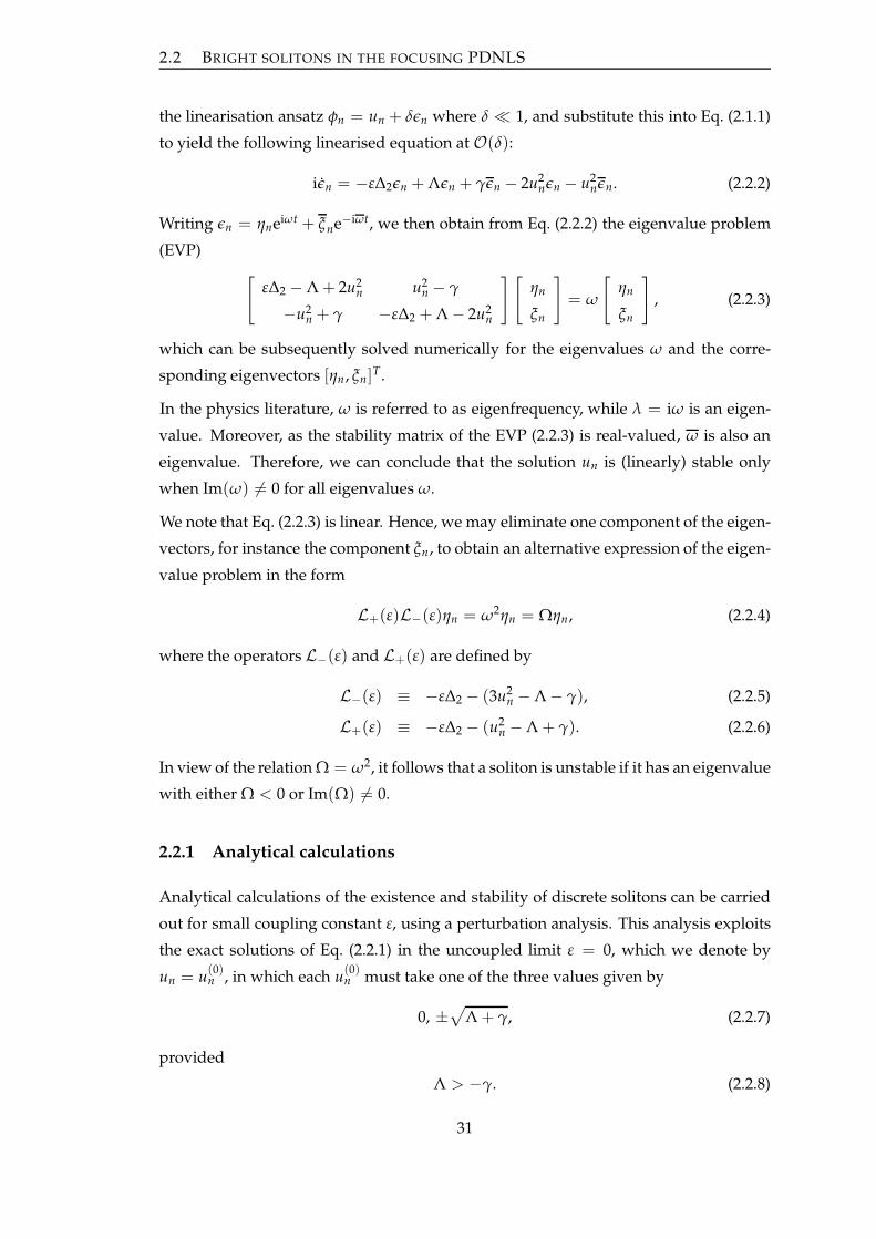
2.2 BRIGHT SOLITONS IN THE FOCUSING PDNLS
the linearisation ansatz φn = un + δǫn where δ ≪ 1, and substitute this into Eq. (2.1.1)
to yield the following linearised equation at O(δ):
iǫn = −ε∆2ǫn + Λǫn + γǫn − 2u2nǫn − u2
nǫn. (2.2.2)
Writing ǫn = ηneiωt + ξne−iωt, we then obtain from Eq. (2.2.2) the eigenvalue problem
(EVP)
[
ε∆2 − Λ + 2u2n u2
n − γ
−u2n + γ −ε∆2 + Λ − 2u2
n
] [
ηn
ξn
]
= ω
[
ηn
ξn
]
, (2.2.3)
which can be subsequently solved numerically for the eigenvalues ω and the corre-
sponding eigenvectors [ηn, ξn]T.
In the physics literature, ω is referred to as eigenfrequency, while λ = iω is an eigen-
value. Moreover, as the stability matrix of the EVP (2.2.3) is real-valued, ω is also an
eigenvalue. Therefore, we can conclude that the solution un is (linearly) stable only
when Im(ω) 6= 0 for all eigenvalues ω.
We note that Eq. (2.2.3) is linear. Hence, we may eliminate one component of the eigen-
vectors, for instance the component ξn, to obtain an alternative expression of the eigen-
value problem in the form
L+(ε)L−(ε)ηn = ω2ηn = Ωηn, (2.2.4)
where the operators L−(ε) and L+(ε) are defined by
L−(ε) ≡ −ε∆2 − (3u2n − Λ − γ), (2.2.5)
L+(ε) ≡ −ε∆2 − (u2n − Λ + γ). (2.2.6)
In view of the relation Ω = ω2, it follows that a soliton is unstable if it has an eigenvalue
with either Ω < 0 or Im(Ω) 6= 0.
2.2.1 Analytical calculations
Analytical calculations of the existence and stability of discrete solitons can be carried
out for small coupling constant ε, using a perturbation analysis. This analysis exploits
the exact solutions of Eq. (2.2.1) in the uncoupled limit ε = 0, which we denote by
un = u(0)n , in which each u
(0)n must take one of the three values given by
0, ±√
Λ + γ, (2.2.7)
provided
Λ > −γ. (2.2.8)
31

2.2 BRIGHT SOLITONS IN THE FOCUSING PDNLS
Solutions of Eq. (2.2.1) for small ε can then be calculated analytically by writing
un = u(0)n + εu
(1)n + ε2u
(2)n + · · · . (2.2.9)
On substituting the above expansion into Eq. (2.2.1) and collecting the terms in succes-
sive powers of ε, one obtains, at O(1) and O(ε), respectively, the equations
(
u(0)n
)3− (Λ + γ)u
(0)n = 0, (2.2.10)
∆2u(0)n − (Λ + γ)u
(1)n + 3u
(1)n
(
u(0)n
)2= 0. (2.2.11)
Together, the above equations give the leading order correction, u(1)n , as
u(1)n =
∆2u(0)n
−3(
u(0)n
)2+ Λ + γ
. (2.2.12)
Because solutions u(0)n at each site n are independent of each other, there will be in-
finitely many combinations for configuration of u(0)n . Here, however, we focus our
attention on configuration of onsite and intersite bright solitons whose the mode struc-
tures in the AC limit ε = 0 are, respectively, of the form
u(0)n =
√Λ + γ, n = 0,
0, otherwise,(2.2.13)
and
u(0)n =
√Λ + γ, n = 0, 1,
0, otherwise.(2.2.14)
In the above configuration, due to the reflection symmetry (2.1.4), we neglect the neg-
ative quantity of the excited site(s).
Next, in studying the stability problem, it is natural to also expand the eigenvector
having component ηn and the eigenvalue Ω in powers of ε, as
ηn = η(0)n + εη
(1)n +O(ε2), Ω = Ω(0) + εΩ(1) +O(ε2). (2.2.15)
Upon substituting this expansion into Eq. (2.2.4) and identifying coefficients of succes-
sive powers of the small parameter ε, we obtain from the equations at O(1) and O(ε)
[
L+(0)L−(0)− Ω(0)]
η(0)n = 0, (2.2.16)
[
L+(0)L−(0)− Ω(0)]
η(1)n = fn, (2.2.17)
where
fn = [(∆2 + 2u(0)n u
(1)n )L−(0) + L+(0)(∆2 + 6u
(0)n u
(1)n ) + Ω(1)]η
(0)n . (2.2.18)
32

2.2 BRIGHT SOLITONS IN THE FOCUSING PDNLS
As L+(0)L−(0) = (3(u(0)n )2 − Λ − γ)((u
(0)n )2 − Λ + γ) represents only a single inde-
pendent quantity for each n, we simply infer that the operator [L+(0)L−(0)− Ω(0)] in
the above equations is self-adjoint.
In the uncoupled limit, ε = 0, the eigenvalue problem is thus simplified to
Ω(0) = L+(0)L−(0), (2.2.19)
from which we conclude that there are two possible eigenvalues, given by
Ω(0)C = Λ2 − γ2, Ω
(0)E = 4(Λ + γ)γ, (2.2.20)
which correspond, respectively, to the solutions u(0)n = 0 (for all n) and u
(0)n = ±√
Λ + γ
(for all n). Note that the expression of Ω(0)C in Eq. (2.2.20) shows that Λ plays an impor-
tant role. When Λ < γ or Λ < −γ, it is clear that 0 is an unstable solution.
Considering onsite and intersite bright soliton solutions then implies that (for ε = 0)
the eigenvalues Ω(0)E and Ω
(0)C have finite and infinite multiplicity, respectively. These
then generate a corresponding discrete and continuous spectrum (phonon band) for
finite positive ε.
To investigate the significance of the continuous spectrum, we introduce a plane-wave
expansion
ηn = aeiκn + be−iκn, (2.2.21)
from which one obtains the dispersion relation
Ω = [2ε(cos κ − 1)− Λ]2 − γ2. (2.2.22)
This in turn shows that the continuous band lies between
ΩL = Λ2 − γ2, when κ = 0, (2.2.23)
and
ΩU = Λ2 − γ2 + 8ε(Λ + 2ε), when κ = π. (2.2.24)
Let us now investigate all the possible cases in the continuous spectrum through the
analysis of the parameter values Λ and γ and their relation (recall that ε and γ have
been set to be positive in the beginning). For Λ > 0, by considering the condition (2.2.8),
there are two cases, i.e., Λ ≥ γ > 0 or γ > Λ > 0. The first case implies that all the
eigenvalues Ω ∈ [ΩL, ΩU ] lie along the positive real axis for all ε which means that
the continuous spectrum does not cause instability. On the contrary, the second case
yields ΩL < 0 which leads to the instability of soliton for all ε. Next, for Λ ≤ 0, we
should require γ > −Λ ≥ 0 due to the condition (2.2.8). The latter case, as in the case
33

2.2 BRIGHT SOLITONS IN THE FOCUSING PDNLS
of γ > Λ > 0, makes ΩL always negative resulting in the instability of soliton for any
value of ε.
We are not interested in the case in which the solitons are already found to be unstable
for all ε. Therefore the range of parameter values Λ and γ which we consider in the
next analysis for onsite and intersite bright solitons is
Λ ≥ γ > 0. (2.2.25)
By this consideration, we only need to examine the stability of the soliton from the
dynamics of the discrete spectrum. For this reason, we also sometimes call the discrete
spectrum the critical eigenvalues.
2.2.1.1 Onsite bright solitons
The existence and stability of a single excited state, i.e., an onsite bright soliton, in the
presence of parametric driving have been considered by Susanto et al. [91]. When ε =
0, as previously explained, this soliton has the leading-order solution (2.2.13). Upon
substituting the values of u(0)n into Eq. (2.2.12), one obtains
u(1)n =
1/√
Λ + γ, n = 0, 1,−1
0, otherwise.(2.2.26)
Thus, for small ε, an onsite bright soliton is given by
un =
√Λ + γ + ε/
√Λ + γ +O(ε2), n = 0,
ε/√
Λ + γ +O(ε2), n = −1, 1,
O(ε2), otherwise.
(2.2.27)
Let us now evaluate the discrete eigenvalues of the above soliton. At ε = 0, there
is only one nonzero excited site. Therefore, from Eq. (2.2.16), an onsite bright soliton
has one leading-order eigenvalue Ω(0)E = 4(Λ + γ)γ corresponding to the normalised
eigenvector with the components η(0)n = 0 for n 6= 0 and η
(0)0 = 1.
To calculate the continuation of the eigenvalue Ω(0)E for nonzero ε, we can consider
Eq. (2.2.17). As the rank of the corresponding operator is not full due to L+(0)L−(0)−Ω
(0)E = 0 at n = 0, we need a solvability condition. From the Fredholm alternative
theorem, we should require that f = col(..., f−1, f0, f1, ...) is orthogonal to the nullspace
of the adjoint of the operator [L+(0)L−(0)− Ω(0)E ]. Nevertheless, the operator is self-
adjoint thus the eigenvector associated with the eigenvalue Ω(0)E is in the nullspace of
the adjoint of the operator (see again Eq. (2.2.16)). Because all the components of the
eigenvector are zero except at site n = 0, this in return, gives f0 = Ω(1) − 8γ = 0 from
34

2.2 BRIGHT SOLITONS IN THE FOCUSING PDNLS
which we deduce that Ω(1) ≡ Ω(1)E = 8γ. Hence the discrete eigenvalue of an onsite
bright soliton is given by
ΩE = 4(Λ + γ)γ + 8γε +O(ε2). (2.2.28)
It was shown by Susanto et al. [91] that the configuration (2.2.27), which is known to be
stable for any value of ε when γ = 0, can be destabilised by parametric driving. Fur-
thermore, it was shown that there are two mechanisms of destabilisation, as sketched
in Fig. 2.1. The two instability scenarios, as illustrated in the figure, are determined
by the relative positions of Ω(0)E and Ω
(0)C , as we now summarise. First, we note that
there is a threshold value1, γth = Λ/5, at which the two leading-order eigenvalues
coincide, so that Ω(0)E = Ω
(0)C . For γ > γth (see lower panel of Fig. 2.1), upon increasing
ε from ε = 0, the instability is caused by the collision of ΩE with ΩU (this leading-to-
instability collision is confirmed after numerical observation); taking ΩE = ΩU then
yields the corresponding approximate critical value
γcr,1 = −2
5Λ − 4
5ε +
1
5
√
9Λ2 + 56εΛ + 96ε2. (2.2.29)
For γ < γth (see upper panel of Fig. 2.1), by contrast, the instability is caused by the
collision of ΩE with an eigenvalue bifurcating from ΩL. However, we assume here that
the bifurcating eigenvalue moves slowly so that it can be represented by ΩL. In this
case, the critical value of γ can be approximated by taking ΩE = ΩL, giving
γcr,2 = −2
5Λ − 4
5ε +
1
5
√
9Λ2 + 16ε(Λ + ε). (2.2.30)
Together, γcr,1 and γcr,2 give approximate boundaries of the instability region in the
(ε, γ)-plane.
2.2.1.2 Intersite bright solitons
The next natural fundamental solution to be considered is an intersite bright soliton,
i.e., a two-excited-site discrete mode. In the uncoupled limit, as presented above,
the mode structure u(0)n is of the form (2.2.14). By substituting the values of u
(0)n into
Eq. (2.2.12), one can show that
u(1)n =
1/(2√
Λ + γ), n = 0, 1,
1/√
Λ + γ, n = −1, 2,
0, otherwise.
(2.2.31)
1There is a typo for this value in Susanto et al. [91].
35

2.2 BRIGHT SOLITONS IN THE FOCUSING PDNLS
Figure 2.1: A sketch of the dynamics of the eigenvalues and the continuous spectrum
of a stable onsite bright soliton in the (Re(Ω),Im(Ω))-plane. The arrows
indicate the direction of movement as the coupling constant ε increases.
Note that a soliton is unstable if there is some Ω with either Ω < 0 or
Im(Ω) 6= 0.
Therefore, an intersite bright soliton for small coupling ε is given by
un =
√Λ + γ + 1
2 ε/√
Λ + γ +O(ε2), n = 0, 1,
ε/√
Λ + γ +O(ε2), n = −1, 2,
O(ε2), otherwise.
(2.2.32)
To study the stability of the intersite bright soliton above, let us first consider the O(1)
equation (2.2.16). Due to the presence of two non-zero excited sites at ε = 0, the soliton
(2.2.32) has at leading order the double eigenvalue Ω(0)E = 4(Λ + γ)γ, which corre-
sponds to the eigenvector having components η(0)n = 0 for n 6= 0, 1, η
(0)0 6= 0, and
η(0)1 6= 0.
The continuation of the eigenvalue Ω(0)E for nonzero coupling ε can be obtained from
Eq. (2.2.17) by applying, as before, a Fredholm solvability condition. Because the eigen-
vector corresponding to the eigenvalue Ω(0)E has zero components except at n = 0, 1,
we only need to require f0 = 0 and f1 = 0, i.e.,
(2Λ + Ω(1))η(0)0 − 2(Λ + 2γ)η
(0)1 = 0, (2.2.33)
(2Λ + Ω(1))η(0)1 − 2(Λ + 2γ)η
(0)0 = 0. (2.2.34)
Our simple calculation then shows η(0)0 = ±η
(0)1 from which we immediately deduce
that the double eigenvalue Ω(0)E splits into two distinct eigenvalues, which are given as
functions of ε by
ΩE,1 = 4(Λ + γ)γ + 4γε +O(ε2), (2.2.35)
ΩE,2 = 4(Λ + γ)γ − 4(Λ + γ)ε +O(ε2). (2.2.36)
36

2.2 BRIGHT SOLITONS IN THE FOCUSING PDNLS
As is the case for onsite discrete solitons, interite bright solitons can also become unsta-
ble. The mechanism of the instability, after confirmation from numerics, is again deter-
mined by the relative positions of Ω(0)E and Ω
(0)C , as sketched in Fig. 2.2. Performing an
analysis corresponding to that in Susanto et al. [91], we find that the two mechanisms
of destabilisation for an onsite discrete soliton also occur here. The two scenarios have
corresponding critical values of γ, which are given as functions of ε by
γcr,1 = −2
5Λ +
2
5ε +
1
5
√
9Λ2 + 52Λε + 84ε2, (2.2.37)
γcr,2 = −2
5Λ − 2
5ε +
1
5
√
9Λ2 + 8Λε + 4ε2, (2.2.38)
which are obtained, respectively, by taking ΩE,2 = ΩU for γ > γth and ΩE,1 = ΩL for
γ < γth.
Figure 2.2: As Fig. 2.1, but for a stable intersite bright soliton.
We emphasise, as is apparent from the sketch shown in Fig. 2.2, that there is another
possible mechanism of destabilisation for γ < γth, namely when ΩE,2 becomes nega-
tive. The third critical choice of parameter values is then obtained by setting ΩE,2 = 0
which gives
γcr,3 = ε. (2.2.39)
Furthermore, by solving γcr,2 = γcr,3 we find that γ = (√
13− 2)Λ/9, which then gives
a more specific domain of γ’s for the two possible scenarios of destabilisation above;
γcr,3 is for γ < (√
13 − 2)Λ/9 and γcr,2 for (√
13 − 2)Λ/9 < γ < γth.
2.2.2 Comparisons with numerical calculations
We have solved the steady-state equation (2.2.1) numerically using a Newton–Raphson
method and analysed the stability of the numerical solution by solving the eigenvalue
problem (2.2.3). In this section, we compare these numerical results with the analytical
37

2.2 BRIGHT SOLITONS IN THE FOCUSING PDNLS
calculations of the previous section. For the sake of simplicity, we set Λ = 1 in all the
illustrative examples. This setting, however, does not lose generality as Λ > 0 can be
scaled out to 1 by the transformation
un → un
√Λ, ε → εΛ and γ → γΛ. (2.2.40)
2.2.2.1 Onsite bright solitons
Comparisons between numerical calculations and analytical approximations for the
case of onsite bright solitons have been fully presented and discussed by Susanto et
al. [91]. For the sake of completeness, we reproduce the results of [91] for the (in)stability
domain of onsite bright solitons in the (ε, γ)-plane in Fig. 2.3 by introducing the colour
representation for the maximum value of |Im(ω)|. Approximations (2.2.29) and (2.2.30)
are also shown there from which we can see that the former gives better prediction for
the occurrence of the instability point than the latter. This is understandable as the
onset of the instability approximated by Eq. (2.2.29) is indeed caused by the collision
of the discrete eigenvalue with the upper band of the continuous spectrum and also
typically occurs for small ε. This is not the case in approximation (2.2.30) where the ac-
tual collision is with an eigenvalue bifurcating from the inner edge of the phonon band
and occurs for relatively large ε. Moreover, for γ < 0, as shown in Fig. 2.3, the onsite
bright soliton is always unstable for all ε. This is still in accordance with our analytical
prediction, i.e., if we set γ to be negative (provided Λ > −γ) in approximate eigen-
value (2.2.28), the eigenvalue ΩE becomes negative for any value of coupling constant
ε.
2.2.2.2 Intersite bright solitons
For the stability of intersite bright solitons, we start by examining the validity of our
analytical prediction for the critical eigenvalues as given by Eqs. (2.2.35) and (2.2.36).
In Fig. 2.4, we present a comparison between the analytical approximation and the nu-
merics for some values of γ, specifically γ = 0.1, 0.18, 0.5, to represent the three possible
cases explained in the previous section. One should notice that the appearance of the
branching curves for each value of γ in the figure manifests the fact (from numerics
and analytics) that the double eigenvalue of an intersite bright soliton splits into two
distinct eigenvalues once the coupling is turned on. The figure reveals the relative ac-
curacy of the small-ε approximations, and we conclude that their range of validity is
wider for the lower branches of each branching curve.
Next we turn to a description of the eigenvalue structure of this intersite configuration
38

2.2 BRIGHT SOLITONS IN THE FOCUSING PDNLS
ε
γ
0 1 2 3 4−0.2
0
0.2
0.4
0.6
0.8
0
0.2
0.4
0.6
0.8
1
1.2Λ=1
Figure 2.3: The (in)stability region of onsite bright solitons in (ε, γ)-space. For each
value of ε and γ, the corresponding colour indicates the maximum value of
|Im(ω)| (over all eigenvalues ω) for the steady-state solution at that point.
Stability is therefore indicated by the region in which Im(ω) = 0, namely
the black region (recall that ω and ω are eigenvalues as the stability matrix
of the EVP (2.2.3) is real-valued). White dashed and dash-dotted lines give
the analytical approximations (2.2.29) and (2.2.30), respectively.
for the three values of γ given above; this is shown in Fig. 2.5, where the left and right
panels respectively present the structure just before and just after the first collision that
results in the mode instability. We now describe the results in more detail for the three
values of γ above.
For γ = 0.1, when ε = 0 the critical eigenvalues ω lie in the gap between the two parts
of the continuous spectrum, and the instability is caused by a collision between one of
the critical eigenvalues and its twin at the origin (see the top panels of Fig. 2.5). For
γ = 0.18, the critical eigenvalues ω also lie in the gap between the two parts of the
continuous spectrum, but the instability in this case is due to a collision between one of
the critical eigenvalues and the inner edge of the continuous spectrum at ω = ±√
ΩL
(see the middle panels of Fig. 2.5). In contrast to the two cases above, for γ = 0.5 the
critical eigenvalues lie beyond the continuous spectrum, and the instability is caused
by a collision between one of the critical eigenvalues and the outer boundary at ω =
±√
ΩU (see the bottom panels of Fig. 2.5). All the numerical results presented here are
in accordance with the sketch shown in Fig. 2.2. Back to Fig. 2.4, the critical eigenvalues
which are most responsible for the instability as illustrated above are shown by the
upper branch for γ = 0.18 (the middle branching curve) and the lower ones for γ = 0.5
and γ = 0.1 (the other branching curves).
39

2.2 BRIGHT SOLITONS IN THE FOCUSING PDNLS
0 0.01 0.02 0.03 0.04 0.05 0.060.4
0.6
0.8
1
1.2
1.4
1.6
1.8
2
ε
|ω|
Λ=1
Figure 2.4: Comparison between the critical eigenvalues of intersite bright solitons ob-
tained numerically (solid lines) and their analytical approximation (dashed
lines). The appearance of the branching curves confirms the fact of the
splitting of the double eigenvalues as ε increases (see text). The upper
and lower branching curves correspond, respectively, to γ = 0.5 and
γ = 0.1, whereas the middle one corresponds to γ = 0.18. The upper and
lower branches of each branching curve is approximated, respectively, by
Eq. (2.2.35) and Eq. (2.2.36); note that these approximations for γ = 0.1 (the
lower branching curve) are indistinguishable from the numerical results.
40

2.3 DARK SOLITONS IN THE DEFOCUSING PDNLS
Numerical solution of the EVP (2.2.3) for intersite bright solitons, for a relatively large
range of ε and γ, give us the (in)stability domain of the bright solitons in the two-
parameter (ε, γ)-plane, which is presented in Fig. 2.6. Again, we use colours to rep-
resent the maximum of |Im(ω)| as a function of ε and γ; thus solitons are stable in
the black region. Our analytical predictions for the occurrence of instability, given by
Eqs. (2.2.37)–(2.2.39), are also shown, respectively, by dash-dotted, dotted and dashed
lines. Particularly for γ < 0, Fig. 2.6 reveals the unstable region of the intersite bright
solitons for all ε. This fact also agrees with our analytical prediction shown by both ΩE,1
in Eq. (2.2.35) and ΩE,2 in Eq. (2.2.36) being negative at any value of ε when driving γ
is negative (provided Λ > −γ).
We now move on the examination of the dynamics of the governing equation (2.1.1) for
an intersite bright soliton. By using a Runge-Kutta time integrator with the perturbed
intersite soliton solution as the initial condition, we show in Fig. 2.7 the numerical evo-
lution of the soliton for the same parameter values as those used in Fig. 2.5, which
corresponds to each of the instability scenarios. We can see from the figure that the
dynamics of the unstable solitons (right panels) manifests itself into different mecha-
nisms. In the top right panel, the soliton’s centre shifts to another site forming an onsite
configuration. In contrast, the typical instability of the unstable soliton in the middle
right panel is in the form of soliton decay, while in the bottom right panel the soliton
collapses into different sites.
2.3 Dark solitons in the defocusing PDNLS
In this section we consider the existence and stability of onsite and intersite dark soli-
tons for the defocusing PDNLS equation. Then a stationary (real-valued and time-
independent) solution un of Eq. (2.1.1) satisfies
− ε∆2un − (Λ + γ)un + u3n = 0. (2.3.1)
To examine the stability of un, we again introduce the linearisation ansatz φn = un +
δǫn, where δ ≪ 1. Substituting this ansatz into the defocusing equation (2.1.1), writing
ǫn = ηneiωt + ξne−iωt and linearising in δ, we find
[
ε∆2 + Λ − 2u2n −u2
n + γ
u2n − γ −ε∆2 − Λ + 2u2
n
] [
ηn
ξn
]
= ω
[
ηn
ξn
]
. (2.3.2)
The eigenvalue problem above can be simplified further as for the focusing case, to the
alternative form
L+(ε)L−(ε)ηn = ω2ηn = Ωηn, (2.3.3)
41

2.3 DARK SOLITONS IN THE DEFOCUSING PDNLS
−2 −1.5 −1 −0.5 0 0.5 1 1.5 2−1
−0.5
0
0.5
1
Re(ω)
Im(ω
)
(a) γ = 0.1, ε = 0.05
−2 −1.5 −1 −0.5 0 0.5 1 1.5 2−1
−0.5
0
0.5
1
Re(ω)
Im(ω
)
(b) γ = 0.1, ε = 0.3
−1.5 −1 −0.5 0 0.5 1 1.5
−0.2
−0.1
0
0.1
0.2
0.3
Re(ω)
Im(ω
)
(c) γ = 0.18, ε = 0.05
−1.5 −1 −0.5 0 0.5 1 1.5
−0.2
−0.1
0
0.1
0.2
0.3
Re(ω)
Im(ω
)
(d) γ = 0.18, ε = 0.18
−2 −1.5 −1 −0.5 0 0.5 1 1.5 2
−0.2
−0.1
0
0.1
0.2
0.3
Re(ω)
Im(ω
)
(e) γ = 0.5, ε = 0.05
−2 −1.5 −1 −0.5 0 0.5 1 1.5 2
−0.2
−0.1
0
0.1
0.2
0.3
Re(ω)
Im(ω
)
(f) γ = 0.5, ε = 0.2
Figure 2.5: The structure of the eigenvalues of intersite bright solitons in the complex
plane for three values of γ, as indicated in the caption of each plot. Left
and right panels depict the eigenvalues of stable and unstable solitons,
respectively.
42

2.3 DARK SOLITONS IN THE DEFOCUSING PDNLS
ε
γ
0 0.1 0.2 0.3 0.4 0.5 0.6 0.7−0.1
0
0.1
0.2
0.3
0.4
0.5
0
0.2
0.4
0.6
0.8
1
1.2
Figure 2.6: As Fig. 2.3, but for intersite bright solitons. Our analytical approximations,
given by Eqs. (2.2.37), (2.2.38) and (2.2.39), are shown as white dash-dotted,
dotted and dashed lines, respectively.
but the operators L±(ε) are now defined as
L−(ε) ≡ −ε∆2 + (3u2n − Λ − γ), (2.3.4)
L+(ε) ≡ −ε∆2 + (u2n − Λ + γ). (2.3.5)
2.3.1 Analytical calculations
To perform analytical calculations of the existence and stability of the dark solitons
for small coupling constant ε, we again use a perturbation analysis. As before, in the
uncoupled limit ε = 0, the exact solutions un = u(0)n at each site n can acquire one of
the three values 0,±√Λ + γ, provided Λ > −γ. By expanding un in powers of ε as in
(2.2.9), we arrive at O(1) and O(ε) equations which, in turn, give the solutions un at
order ε as
u(1)n =
∆2u(0)n
3(
u(0)n
)2− (Λ + γ)
. (2.3.6)
In this section, we consider onsite and intersite dark solitons where the respective con-
figurations in the AC limit ε = 0 are given by
u(0)n =
−√Λ + γ, n = −1,−2, . . .,
0, n = 0,√
Λ + γ, n = 1, 2, . . .,
(2.3.7)
43
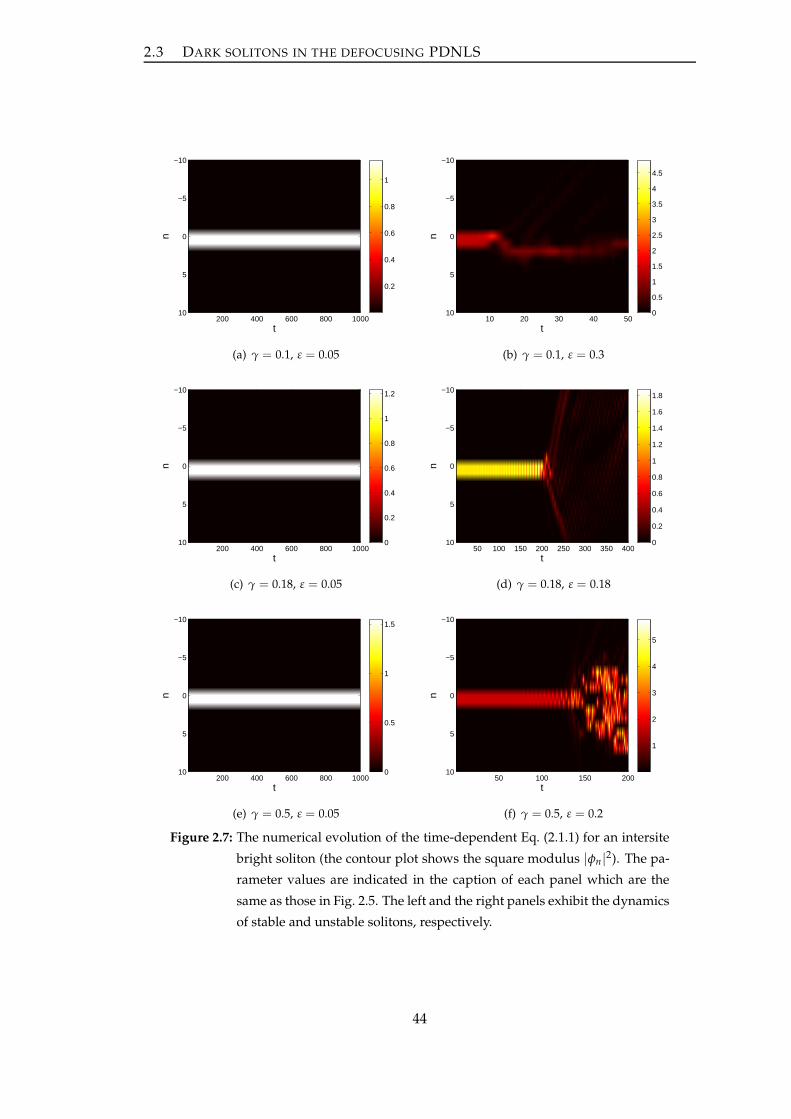
2.3 DARK SOLITONS IN THE DEFOCUSING PDNLS
t
n
200 400 600 800 1000
−10
−5
0
5
10
0.2
0.4
0.6
0.8
1
(a) γ = 0.1, ε = 0.05
t
n
10 20 30 40 50
−10
−5
0
5
10 0
0.5
1
1.5
2
2.5
3
3.5
4
4.5
(b) γ = 0.1, ε = 0.3
t
n
200 400 600 800 1000
−10
−5
0
5
10 0
0.2
0.4
0.6
0.8
1
1.2
(c) γ = 0.18, ε = 0.05
t
n
50 100 150 200 250 300 350 400
−10
−5
0
5
10 0
0.2
0.4
0.6
0.8
1
1.2
1.4
1.6
1.8
(d) γ = 0.18, ε = 0.18
t
n
200 400 600 800 1000
−10
−5
0
5
10 0
0.5
1
1.5
(e) γ = 0.5, ε = 0.05
t
n
50 100 150 200
−10
−5
0
5
10
1
2
3
4
5
(f) γ = 0.5, ε = 0.2
Figure 2.7: The numerical evolution of the time-dependent Eq. (2.1.1) for an intersite
bright soliton (the contour plot shows the square modulus |φn|2). The pa-
rameter values are indicated in the caption of each panel which are the
same as those in Fig. 2.5. The left and the right panels exhibit the dynamics
of stable and unstable solitons, respectively.
44

2.3 DARK SOLITONS IN THE DEFOCUSING PDNLS
and
u(0)n =
−√Λ + γ, n = 0,−1, . . .,
√Λ + γ, n = 1, 2, . . ..
(2.3.8)
Next, to study the eigenvalue(s) of the dark soliton analytically, we again expand ηn
and Ω in powers of ε as in (2.2.15), and hence obtain from Eq. (2.3.3), at O(1) and O(ε),
respectively, the equations
[
L+(0)L−(0)− Ω(0)]
η(0)n = 0, (2.3.9)
and[
L+(0)L−(0)− Ω(0)]
η(1)n = fn, (2.3.10)
where
fn = [(∆2 − 2u(0)n u
(1)n )L−(0) + L+(0)(∆2 − 6u
(0)n u
(1)n ) + Ω(1)]η
(0)n . (2.3.11)
As in bright solitons, the operator [L+(0)L−(0)− Ω(0)] is self-adjoint.
Performing a stability analysis as before, we firstly investigate the significance of con-
tinuous spectrum for a dark soliton by substituting a plane-wave expansion (2.2.21)
into Eq. (2.3.3). From this, we find the dispersion relation for a dark soliton to be
Ω = [2ε(cos κ − 1)− (Λ + 2γ)]2 − Λ2, (2.3.12)
and so the continuous band lies between
ΩL = 4(Λ + γ)γ, when κ = 0, (2.3.13)
and
ΩU = 4(Λ + γ)γ + 8ε(Λ + 2γ + 2ε), when κ = π. (2.3.14)
Our analysis shows that there are only three possibilities for parameter values Λ and
γ in the continuous spectrum above, i.e., either Λ ≥ γ > 0, γ > Λ > 0 or γ > −Λ ≥ 0
(note that the latter is for Λ ≤ 0). For all cases, we can check that all the eigenvalues in
[ΩL, ΩU] are real positive for any value of ε which means that the continuous spectrum
does not create any instability. In this section, however, we restrict ourselves to the first
case only to make the same treatment with the focusing PDNLS.
45

2.3 DARK SOLITONS IN THE DEFOCUSING PDNLS
2.3.1.1 Onsite dark solitons
The configuration of an onsite dark soliton at ε = 0 is given by (2.3.7). Upon substitut-
ing this into Eq. (2.3.6), we obtain the leading order correction, u(1)n , as
u(1)n =
0, n = −2,−3, . . .,
1/(2√
Λ + γ), n = −1,
0, n = 0,
−1/(2√
Λ + γ), n = 1,
0, n = 2, 3, . . ..
(2.3.15)
Therefore, with errors of order ε2, an onsite dark soliton is given by
un =
−√Λ + γ, n = −2,−3, . . .,
−√Λ + γ + 1
2 ε/√
Λ + γ, n = −1,
0, n = 0,√
Λ + γ − 12 ε/
√Λ + γ, n = 1,
√Λ + γ, n = 2, 3, . . ..
(2.3.16)
For this configuration, we have
L+(0)L−(0) =
Λ2 − γ2, n = 0,
4(Λ + γ)γ, n 6= 0.(2.3.17)
From Eq. (2.3.9), we then deduce that at ε = 0 the eigenvalues of onsite discrete dark
solitons are given by Ω(0)C = 4(Λ + γ)γ and Ω
(0)E = Λ2 − γ2 which, respectively, be-
come the continuous and discrete spectrum for nonzero ε. The eigenvalue Ω(0)E has the
normalised eigenvector whose components are η(0)n = 0 for n 6= 0 and η
(0)0 = 1.
Because the continuous spectrum does not contribute to the instability of the soliton,
the eigenvalue Ω(0)E must be taken into account to examine the stability. To do so,
we need to find the continuation of the eigenvalue Ω(0)E for nonzero ε which can be
calculated from Eq. (2.3.10). But, the coefficient of η(1)n which is given by
L+(0)L−(0)− Ω(0) =
0, n = 0,
4Λγ − Λ2 + 5γ2, n 6= 0,(2.3.18)
leads to the rank deficiency in operator L ≡ [L+(0)L−(0)− Ω(0)]. Therefore we need
a solvability condition, i.e., the nullspace of the adjoint of L, which is the eigenvector
corresponding to the eigenvalue Ω(0)E due to the self-adjointness of L, is orthogonal to
f = col(..., f−1, f0, f1, ...). Because the components of the eigenvector are zero except at
site n = 0, we only require f0 = 4Λ + Ω(1) = 0 which then gives Ω(1) ≡ Ω(1)E = −4Λ.
Hence the discrete eigenvalue of an onsite dark soliton for small ε is
ΩE = Λ2 − γ2 − 4Λε +O(ε2). (2.3.19)
46

2.3 DARK SOLITONS IN THE DEFOCUSING PDNLS
Initially, i.e., for ε = 0, the relative positions of the eigenvalue and the continuous
spectrum can be divided into two cases, according to whether γ ≷ γth = Λ/5 (recall
that the threshold value γth is obtained by taking Ω(0)E = Ω
(0)C ). When ε = 0 and γ < γth
(γ > γth) the eigenvalue (2.3.19) will be above (below) the continuous spectrum, as
sketched in Fig. 2.8. These relative positions determine the instability mechanism for
an onsite dark soliton, as we now describe.
Figure 2.8: As Fig. 2.1, but for a stable onsite dark soliton.
For γ < γth, after numerical observations, the instability is due to a collision between
the eigenvalue (2.3.19) and ΩU , which approximately occurs when γ = γcr,1, where
γcr,1 = −2
5Λ − 8
5ε +
1
5
√
9Λ2 − 28Λε − 16ε2. (2.3.20)
Note that for small ε, this critical value is meaningful only when ε ≤ 9Λ/(14 + 2√
85).
For γ > γth, the instability is caused by the eigenvalue (2.3.19) becoming negative,
which occurs when γ = γcr,2, where
γcr,2 =√
Λ2 − 4Λε. (2.3.21)
This value is meaningful only when ε ≤ Λ/4.
Furthermore, if we include terms up to O(ε2), we obtain
ΩE = Λ2 − γ2 − 4Λε + 6ε2 +O(ε3) (2.3.22)
as the eigenvalue of an onsite discrete dark soliton. Using this expression, we find the
critical value of γ indicating the onset of instability as
γ′cr,1 = −2
5Λ − 8
5ε +
1
5
√
9Λ2 − 28Λε + 14ε2, (2.3.23)
for γ < γth, and
γ′cr,2 =
√
Λ2 − 4Λε + 6ε2, (2.3.24)
for γ > γth. For small ε, γ′cr,1 above is defined on ε ≤ (1 −
√70/14)Λ.
47

2.3 DARK SOLITONS IN THE DEFOCUSING PDNLS
2.3.1.2 Intersite dark solitons
The leading-order solution of an intersite dark soliton is given by the configuration (2.3.8)
and the next correction can be obtained from Eq. (2.3.6) resulting
u(1)n =
0, n = −2,−3, . . .,
1/√
Λ + γ, n = −1,
−1/√
Λ + γ, n = 0,
0, n = 1, 2, . . ..
(2.3.25)
Hence, an intersite discrete dark soliton is given, with errors of O(ε2), by
un =
−√Λ + γ, n = −2,−3, . . .,
−√Λ + γ + ε/
√Λ + γ, n = −1,
√Λ + γ − ε/
√Λ + γ, n = 0,
√Λ + γ, n = 1, 2, . . ..
(2.3.26)
Starting from Eq. (2.3.9), we then find
L+(0)L−(0) = 4(Λ + γ)γ for all n, (2.3.27)
from which we deduce that there is a single leading-order eigenvalue, given by Ω(0) =
4(Λ + γ)γ, with infinite multiplicity. This eigenvalue then expands to form the contin-
uous spectrum for nonzero ε.
From the fact of a single eigenvalue above, we cannot say anything about the discrete
eigenvalue(s) yet. However, we still can calculate its continuation as the coupling con-
stant is turned on, which can be carried out from Eq. (2.3.10). Because
L+(0)L−(0)− Ω(0) = 0 for all n, (2.3.28)
the solvability condition for Eq. (2.3.10) requires fn = 0 for all n. A simple calculation
then yields
fn =
[
4Λ + 16γ + (2Λ + 4γ)∆2 + Ω(1)]
η(0)n , n = −1, 0,
[
(2Λ + 4γ)∆2 + Ω(1)]
η(0)n , n 6= −1, 0.
(2.3.29)
Notice that the eigenvector for a localised mode in which there is only one eigenvalue
with infinite multiplicity is also localised and decaying exponentially (see, e.g., Baesens
et al. [103] for a justification). Thus, a suitable ansatz for η(0)n can be chosen as
η(0)n =
Aec(n+3/2), n ≤ −2,
A0, n = −1,
B0, n = 0,
Be−c(n+3/2), n ≥ 1,
(2.3.30)
48

2.3 DARK SOLITONS IN THE DEFOCUSING PDNLS
for A, A0, B0, B 6= 0 and c > 0. Substituting this ansatz into Eq. (2.3.29) and imposing
the solvability condition fn = 0 for all n, we arrive at the following equations
Ae−c/2[(2Λ + 4γ)(e−c − 2) + Ω(1)] + A0(2Λ + 4γ) = 0, n = −2,
A0(8γ + Ω(1)) + B0(2Λ + 4γ) + A(2Λ + 4γ)e−c/2 = 0, n = −1,
B0(8γ + Ω(1)) + A0(2Λ + 4γ) + B(2Λ + 4γ)e−5c/2 = 0, n = 0,
Be−5c/2[(2Λ + 4γ)(e−c − 2) + Ω(1)] + B0(2Λ + 4γ) = 0, n = 1,
(2Λ + 4γ)(ec − 2 + e−c) + Ω(1) = 0, n 6= −1, 0.
(2.3.31)
Our analysis of the first four equations above shows that either A0 = B0 or A0 = −B0
from which we obtain, respectively, either
c = ln
(
3Λ + 10γ
Λ + 2γ
)
, Ω(1) =−8(Λ + 4γ)2
3Λ + 10γ, (2.3.32)
or
c = ln
(
Λ + 6γ
Λ + 2γ
)
, Ω(1) =−32γ2
Λ + 6γ. (2.3.33)
Therefore, the bifurcating discrete eigenvalues of an intersite dark soliton for small ε
are respectively given by
ΩE,1 = 4(Λ + γ)γ − 8(Λ + 4γ)2
3Λ + 10γε +O(ε2), (2.3.34)
ΩE,2 = 4(Λ + γ)γ − 32γ2
Λ + 6γε +O(ε2). (2.3.35)
In the absence of parametric driving (γ = 0) and for Λ = 1, our results agree with that
reported by Pelinovsky & Kevrekidis [90]. One should notice that in the AC limit ε = 0
the above eigenvalues correspond, respectively, to the following normalised eigenvec-
tors
η(0)n =
2√
(Λ+3γ)(Λ+4γ)Λ+2γ
(
3Λ+10γΛ+2γ
)n, n ≤ −2,
2√
(Λ+3γ)(Λ+4γ)3Λ+10γ , n = −1,
2√
(Λ+3γ)(Λ+4γ)3Λ+10γ , n = 0,
2√
(Λ+3γ)(Λ+4γ)3Λ+10γ
(
3Λ+10γΛ+2γ
)−n, n ≥ 1,
(2.3.36)
and
η(0)n =
2√
γ(Λ+4γ)Λ+2γ
(
Λ+6γΛ+2γ
)n, n ≤ −2,
2√
γ(Λ+4γ)Λ+6γ , n = −1,
− 2√
γ(Λ+4γ)Λ+6γ , n = 0,
− 2√
γ(Λ+4γ)Λ+6γ
(
Λ+6γΛ+2γ
)−n, n ≥ 1.
(2.3.37)
Let us now analyse the above discrete eigenvalues. From Eq. (2.3.35) one can show that
when ε > 0 the eigenvalue ΩE,2 is always less than ΩL. As ε increases, both ΩE,1 and
49

2.3 DARK SOLITONS IN THE DEFOCUSING PDNLS
Figure 2.9: As Fig. 2.1, but for a stable intersite dark soliton.
ΩE,2 decrease to zero but ΩE,1 < ΩE,2 (note that ΩE,2 decreases more slowly than ΩE,1).
Therefore, we conclude that the instability may be due to ΩE,1 becoming negative as
illustrated in Fig. 2.9. Equating ΩE,1 = 0 yields the critical values
εcr =γ(3Λ + 10γ)(Λ + γ)
(Λ + 4γ)2, (2.3.38)
which approximate the onset of instability.
2.3.2 Comparison with numerical computations
We now compare our analytical results with corresponding numerical calculations. As
for bright solitons, for illustrative purposes we set Λ = 1. Again, such a setting is with-
out loss of generality because Λ > 0 can be scaled to be 1 by transformation (2.2.40).
2.3.2.1 Onsite dark solitons
We start by checking the validity of our analytical approximation for the critical eigen-
value. As explained above, the change in the position of the eigenvalues relative to
the continuous spectrum at ε = 0 occurs at γ = 1/5. Therefore we consider two val-
ues γ = 0.1 and γ = 0.6, representing both cases. Figure 2.10 depicts a comparison
between our analytical result (2.3.19) and the numerical computations, from which we
conclude that the prediction is quite accurate for small ε. The accuracy can be improved
if one includes further orders in the perturbative expansion (2.3.22); this improvement
is shown in the same figure by the dotted line.
The eigenvalue structure of onsite dark solitons for the two values of γ used above is
depicted in Fig. 2.11; left and right panels refer respectively to conditions just before
and just after a collision resulting in an instability. As sketched in Fig. 2.8, for γ = 0.1
the instability is caused by a collision between the critical eigenvalue and the upper
edge of the continuous spectrum. On the other hand, when γ = 0.6 the instability
is caused by a collision between the critical eigenvalue and its twin at the origin (see
the bottom panels of Fig. 2.11). In the latter case we notice that there is an eigenvalue
bifurcating from the lower edge of the continuous spectrum.
50

2.3 DARK SOLITONS IN THE DEFOCUSING PDNLS
0 0.01 0.02 0.03 0.04 0.05 0.06 0.07 0.080.5
0.6
0.7
0.8
0.9
1
1.1
ε
|ω|
0.042 0.044 0.0460.68
0.685
ε
|ω|
Figure 2.10: Comparisons between the critical eigenvalue for on-site dark solitons ob-
tained numerically (solid lines) and analytically using Eq. (2.3.19) (dashed
lines) for γ = 0.1 (upper curves) and γ = 0.6 (lower curves). An approx-
imation that explicitly includes the next term in expansion Eq. (2.3.22) is
also plotted (dotted lines).
We now proceed to evaluate the (in)stability region of this solution in (ε, γ)-space.
We show in Fig. 2.12 the maximum of the imaginary part of the eigenvalue, together
with our approximation to the (in)stability boundary. The white solid line represents
Eq. (2.3.21), corresponding to the instability caused by the collision with the continuous
spectrum. Equation (2.3.20) is represented by the white dash-dotted line, which corre-
sponds to the other instability mechanism. In addition, white dashed and dotted lines
show, respectively, Eqs. (2.3.24) and (2.3.23), where a better analytical approximation is
obtained.
An important observation from Fig. 2.12 is that there is an interval of values of γ in
which the onsite dark soliton is always stable, for any value of the coupling constant
ε (numerically, it is 0.2 < γ < 0.335). This indicates that a parametric driving can
fully suppress the oscillatory instability reported for the first time by Johansson &
Kivshar [87]. One can also check from Fig. 2.12 that for γ < 0 the onsite dark soliton
is always unstable. In fact, contribution for such instability comes from the lower band
of the continuous spectrum at ω = ±√
ΩL (see Eq. (2.3.13)) which becomes purely
imaginary when γ < 0 (on condition Λ > −γ).
Next, to confirm our stability findings above, we present in Fig. 2.13 the numerical evo-
lution of onsite dark solitons which correspond to the stability and instability modes in
the respective left and right panels of Fig. 2.11. The typical dynamical behaviour of the
51

2.3 DARK SOLITONS IN THE DEFOCUSING PDNLS
−1.5 −1 −0.5 0 0.5 1 1.5−1
−0.5
0
0.5
1
Re(ω)
Im(ω
)
(a) γ = 0.1, ε = 0.02
−1.5 −1 −0.5 0 0.5 1 1.5−1
−0.5
0
0.5
1
Re(ω)
Im(ω
)
(b) γ = 0.1, ε = 0.2
−3 −2 −1 0 1 2 3−0.5
0
0.5
Re(ω)
Im(ω
)
(c) γ = 0.6, ε = 0.01
−3 −2 −1 0 1 2 3−0.5
0
0.5
Re(ω)
Im(ω
)
(d) γ = 0.6, ε = 1
Figure 2.11: The eigenvalue structure of on-site dark solitons for several values of γ
and ε, as indicated in the caption of each panel.
52

2.3 DARK SOLITONS IN THE DEFOCUSING PDNLS
ε
γ
0 0.5 1 1.5 2−0.2
0
0.2
0.4
0.6
0.8
1
0.02 0.04 0.06 0.08 0.1
0
0.05
0.1
0.15
0
0.2
0.4
0.6
0.8
1Λ=1
Figure 2.12: The (in)stability region of onsite dark solitons in the two-parameter (ε, γ)-
space. The white solid and dashed lines respectively give the analytical
approximations Eq. (2.3.21) and (2.3.24). White dash-dotted and dotted
lines show Eqs. (2.3.20) and (2.3.23); note that these curves are indistin-
guishable in this plot.
unstable soliton in the top right panel of Fig. 2.13 is in the form of soliton destruction of
which the centre then eventually shifts to the other site, while, interestingly, in the bot-
tom right panel the unstable soliton becomes a discrete breather where the amplitude
is alternately changed between the two neighbouring sites.
2.3.2.2 Intersite dark solitons
Now we examine intersite dark solitons. First, Fig. 2.14 shows the analytical predic-
tion for the critical eigenvalues, given by Eqs. (2.3.34)-(2.3.35), compared to the cor-
responding numerical results. One should not be surprised by the appearance of the
branching curves in the figure as they reveal the bifurcation of the critical eigenvalues
from the inner edge of the continuous spectrum as soon as ε is turned on from which
they then split into two distinct eigenvalues. We see that the approximations given by
Eqs. (2.3.34)-(2.3.35) are in good agreement with the numerics. The range of validity of
these approximations is wider for the upper branches in each branching curve.
The analytical calculation of the eigenvalues (2.3.34) and (2.3.35) is based on the formu-
lation of the leading-order eigenvectors (2.3.36) and (2.3.37), respectively. The compar-
isons between the approximate eigenvectors and the numerical results, as presented in
Fig. 2.15, show that our theoretical prediction is excellent.
53

2.3 DARK SOLITONS IN THE DEFOCUSING PDNLS
t
n
100 200 300 400 500
−10
−5
0
5
10 0
0.2
0.4
0.6
0.8
1
(a) γ = 0.1, ε = 0.02
t
n
100 200 300 400 500
−10
−5
0
5
10
0.2
0.4
0.6
0.8
1
1.2
(b) γ = 0.1, ε = 0.2
t
n
200 400 600 800 1000
−10
−5
0
5
10 0
0.2
0.4
0.6
0.8
1
1.2
1.4
1.6
(c) γ = 0.6, ε = 0.01
t
n
200 400 600 800 1000
−10
−5
0
5
10
0.2
0.4
0.6
0.8
1
1.2
1.4
1.6
(d) γ = 0.6, ε = 1
Figure 2.13: The numerical integration of Eq. (2.1.1) for the onsite dark solitons corre-
sponding to the mode (in)stability in Fig. 2.11.
54

2.3 DARK SOLITONS IN THE DEFOCUSING PDNLS
0 0.02 0.04 0.06 0.08 0.10
0.5
1
1.5
2
2.5
3
ε
|ω|
Λ=1
Figure 2.14: Comparisons between the critical eigenvalue of intersite dark solitons ob-
tained numerically (solid lines) and analytically (dashed lines) for two
values of γ. The upper branching curves correspond to γ = 0.8 while the
lower ones to γ = 0.1. The analytical approximations for the lower-upper
branches in each branching curve are given by Eqs. (2.3.34)-(2.3.35).
Next, we plot in Fig. 2.16 the eigenvalue structure of this configuration for the two
values γ = 0.1, 0.8. The mechanism of instability explained in the section above can
be seen clearly in the top panels of Fig. 2.16, i.e., the instability is caused by a collision
between one of the critical eigenvalues and its twin at the origin (in Fig. 2.14, this eigen-
value corresponds to the lower branch of the lower branching curves). It is interesting
to note that a parametric driving can also fully suppress the oscillatory instability of an
intersite dark soliton. As shown in the bottom panels of Fig. 2.16, there are values of
the parameter γ for which no instability-inducing collision ever occurs.
The (in)stability region of this configuration as well as the analytical prediction for the
onset of instability are summarised in Fig. 2.17. We see from the figure that for any ε
and γ > 0.305 an intersite dark soliton is always stable. By contrast, we also see that
the intersite dark soliton is always unstable for γ < 0. The instability in this case is
caused by the fact, as in onsite dark solitons, that the lower band of the continuous
spectrum (ω = ±√
ΩL) lies on the imaginary axis.
As a confirmation for the (in)stability scenarios discussed above, we depict in Fig. 2.18
the numerical dynamics of stable and unstable intersite dark solitons which correspond
to stable and unstable modes of the eigenvalues in the top panels of Fig. (2.16). Inter-
estingly, the unstable soliton eventually travels with the negative velocity which seem-
ingly remains constant. This leading-to-travelling instability is similar to that reported
55

2.3 DARK SOLITONS IN THE DEFOCUSING PDNLS
−20 −10 0 10 20−0.1
0
0.1
0.2
0.3
0.4
0.5
0.6
0.7
n
η n(0)
(a) γ = 0.1, A = B
−20 −10 0 10 20−0.5
−0.4
−0.3
−0.2
−0.1
0
0.1
0.2
0.3
0.4
0.5
nη n(0
)
(b) γ = 0.1, A = −B
−20 −10 0 10 20−0.1
0
0.1
0.2
0.3
0.4
0.5
0.6
0.7
0.8
n
η n(0)
(c) γ = 0.8, A = B
−20 −10 0 10 20−0.8
−0.6
−0.4
−0.2
0
0.2
0.4
0.6
0.8
n
η n(0)
(d) γ = 0.8, A = −B
Figure 2.15: Comparisons between the eigenvectors corresponding to the discrete
eigenvalues of an intersite dark soliton in the uncoupled limit ε = 0 ob-
tained numerically (solid lines) and analytically (circles) for two values
of γ as indicated in the caption for each panel. The analytical approx-
imations are obtained from Eqs. (2.3.36) (left panels) and (2.3.37) (right
panels).
56

2.3 DARK SOLITONS IN THE DEFOCUSING PDNLS
−3 −2 −1 0 1 2 3−0.5
0
0.5
Re(ω)
Im(ω
)
(a) γ = 0.1, ε = 0.05
−3 −2 −1 0 1 2 3−0.5
0
0.5
Re(ω)
im(ω
)
(b) γ = 0.1, ε = 0.5
−8 −6 −4 −2 0 2 4 6 8−1
−0.5
0
0.5
1
Re(ω)
Im(ω
)
(c) γ = 0.8, ε = 0.5
−8 −6 −4 −2 0 2 4 6 8−1
−0.5
0
0.5
1
Re(ω)
Im(ω
)
(d) γ = 0.8, ε = 2
Figure 2.16: The eigenvalue structure of intersite dark solitons with parameter values
as indicated in the caption for each panel.
ε
γ
0 0.5 1 1.5−0.2
−0.1
0
0.1
0.2
0.3
0.4
0.5
0.6
0
0.1
0.2
0.3
0.4
0.5
0.6
0.7
0.8
0.9
1Λ=1
Figure 2.17: As Fig. 2.12, but for an intersite dark soliton. The white dashed line is our
analytical approximation (2.3.38).
57

2.4 PDNLS IN ELECTROMECHANICAL RESONATORS
t
n
200 400 600 800 1000
−10
−5
0
5
10
1.01
1.02
1.03
1.04
1.05
1.06
1.07
1.08
1.09
1.1
t
n
200 400 600 800 1000
−50
0
50
0.2
0.4
0.6
0.8
1
1.2
Figure 2.18: As Fig. 2.13, but for an intersite dark soliton with γ = 0.1. The left and
right panels depict the evolution of a stable dark soliton with ε = 0.05
and an unstable one with ε = 0.5, respectively.
by Fitrakis et al. [86] for the case of undriven cubic and saturable DNLS equations.
2.4 PDNLS in electromechanical resonators
In this section, we discuss the use of parametrically driven DNLS equation in describ-
ing the dynamics of MEMS and NEMS resonators. We have provided a brief review of
MEMS and NEMS resonators in Section 1.3.2.2.
2.4.1 The model and the reduction
Motivated by a recent experiment of Buks and Roukes [51] that succeeded in fabricating
and exciting an array of MEMS and measuring oscillations of the resonators, here we
consider the equation (Kenig et al. [58])
ϕn = D∆2 ϕn − [1 − H cos(2ωpt)]ϕn ± ϕ3n, (2.4.1)
which governs the oscillation amplitude of such an array. Equation (2.4.1) is a simpli-
fied model of that discussed by Lifshitz & Cross [57], subject to an assumption that the
piezoelectric parametric drive is applied directly to each oscillator as recently demon-
strated by Masmanidis et al. [104]. The variable ϕn represents the oscillation ampli-
tude of the nth oscillator from its equilibrium position, D is a dc electrostatic nearest-
neighbour coupling term, H is a small ac component with frequency 2ωp responsible
for the parametric driving, ∆2 ϕn = ϕn+1 − 2ϕn + ϕn−1 is the discrete Laplacian, the dot
denotes the derivative with respect to time t (notice that time t here is not the same as
time t in Eq. (2.1.1)), and the ‘plus’ and ‘minus’ signs of the cubic term correspond to
58

2.4 PDNLS IN ELECTROMECHANICAL RESONATORS
‘softening’ and ‘stiffening’ nonlinearities, respectively. Here, we assume ideal oscilla-
tors, so there is no damping present. The creation, stability and interactions of ILMs
in Eq. (2.4.1) with low damping and in the strong-coupling limit or slowly varying so-
lutions, have been investigated by Kenig et al. [58]. Here, we extend that study to the
case of small coupling parameter D or strongly localised solutions.
In performing our analysis to the governing equation (2.4.1), we introduce a small pa-
rameter δ ≪ 1 and assume that the following scalings hold:
D = δ2D, H = δ2H, ωp = 1 + δ2ωp. (2.4.2)
Note that the leading order term for ωp in the above equation is 1 due to it being the
natural frequency of the unforced system linearised about φn = 0, namely φn = −φn.
We then expand each ϕn in powers of δ, with the leading-order term being of the form
ϕn ∼ δ(
ψn(T1, T2, T3, . . . )e−iT0 + ψn(T1, T2, T3, . . . )eiT0
)
, (2.4.3)
with slow temporal variables Tn = δnt. Substituting Eq. (2.4.3) into Eq. (2.4.1) and
equating coefficients of powers of δ then yield
O(δ2) : 2i∂ψn
∂T1e−iT0 + c.c. = 0, (2.4.4)
O(δ3) :
(
2i∂ψn
∂T2− ∂2ψn
∂T21
+ D∆2ψn +1
2Hψne−2iωpT2 ± 3|ψn|2ψn
)
e−iT0
+
(
1
2Hψne−2iωpT2 ± ψ3
n
)
e−3iT0 + c.c. = 0, (2.4.5)
where c.c. stands for the complex conjugate of the preceding expression.
Because ∂2ψn/∂T21 = 0, i.e., from Eq. (2.4.4), the terms at O(e−iT0) in Eq. (2.4.5) then give
the following equation for ψn (see Kivshar [105] and Remoissenet [106] for a related
reduction method)
− 2iψn = D∆2ψn +1
2Hψne−2iωpT2 ± 3|ψn|2ψn, (2.4.6)
where the overdot now denotes the derivative with respect to T2. Correction terms in
Eq. (2.4.3) are O(δe±i(k+1)T0 , δ3e±i(k−1)T0), with k ∈ Z+. A justification of this rotating-
wave-type approximation can be obtained in, e.g., Kosevich & Corso [108].
Using the following scalings2
D = 3ε, H = ∓6γ, ωp = ∓3Λ/2, (2.4.7)
and then writing ψn(T2) = φn(T2)e±3iΛT2/2, Eq. (2.4.6) can be rewritten as
− 2
3iφn = ε∆2φn ∓ Λφn ∓ γφn ± |φn|2φn. (2.4.8)
2There is a typo in the scaling of H in Syafwan et al. [107].
59

2.4 PDNLS IN ELECTROMECHANICAL RESONATORS
Finally by taking T2 = 23 t, we find that the equation above becomes the parametri-
cally driven discrete nonlinear Schrödinger (PDNLS) equation as written in Eq. (2.1.1),
where the overdot denotes the derivative with respect to t. The softening and stiffen-
ing nonlinearities of Eq. (2.4.1) correspond, respectively, to the focusing and defocusing
cases in the PDNLS (2.1.1). The continuum limit of Eq. (2.1.1), i.e., φn ≈ φ, ε∆2φn ≈ ∂2xφ,
was considered by Kenig et al. [58] from Eq. (2.4.1) and by Barashenkov et al. [109] from
a parametrically driven sine-Gordon equation by considering slowly varying solitons.
2.4.2 Numerical integrations
In Sections 2.2 and 2.3, we discussed the existence and the stability of localised modes
of the PDNLS equation (2.1.1). In this section, we confirm the relevance of our findings
through solving numerically the time-dependent equation (2.4.1). We use a Runge–
Kutta integration method, with the initial condition ϕn = 2δun and ϕn = 0, where un
is the static solution of the PDNLS (2.1.1) and δ is the small parameter of Section 2.4.1.
Throughout this section, we use the illustrative value δ = 0.2. Recall that we have
made scalings to the parameters as
D = 3δ2ε, H = ∓6δ2γ, ωp = 1 ∓ 3δ2Λ/2. (2.4.9)
In the left and right panels of Fig. 2.19, we plot the numerical evolution of a stable and
unstable onsite bright soliton, respectively. From the top right panel of the figure, we
note that a parametric driving seems to destroy an unstable soliton. This observation
is similar to the corresponding observation for the dynamics of an unstable soliton in
the DNLS equation (2.1.1) reported by Susanto et al. [91]. In the bottom right panel,
we present another case of unstable dynamics for a relatively large parametric driving
amplitude γ, where the bright soliton is seemingly still preserved up to some time and
then suddenly decays.
In Fig. 2.20 we present the numerical evolution of intersite bright solitons for the same
parameter values as those in Fig. 2.5, corresponding to each of the instability scenarios.
From the panels in this figure, we see that the typical outcome of the instability is that
the profile of the soliton changes to a different form. In the top and middle right panels,
the soliton becomes an onsite breather with the latter changing its centre position alter-
nately. In the bottom right panel, the unstable soliton becomes two-separated-excited
sites with radiation forming a breather.
We have also examined the dynamics of onsite dark solitons in the Klein–Gordon sys-
tem (2.4.1). We show in Fig. 2.21 the numerical evolution of a solution with the eigen-
value structure illustrated in Fig. 2.11. The instability of an unstable onsite dark soliton
60

2.4 PDNLS IN ELECTROMECHANICAL RESONATORS
t
n
200 400 600 800 1000 1200 1400 1600
−10
−8
−6
−4
−2
0
2
4
6
8
10 0
0.02
0.04
0.06
0.08
0.1
0.12
0.14
0.16
0.18
0.2
(a) γ = 0.1, ε = 0.1
tn
200 400 600 800
−10
−8
−6
−4
−2
0
2
4
6
8
10 0
0.05
0.1
0.15
0.2
0.25
0.3
0.35
0.4
0.45
(b) γ = 0.1, ε = 1
t
n
200 400 600 800 1000 1200 1400 1600
−10
−8
−6
−4
−2
0
2
4
6
8
10 0
0.05
0.1
0.15
0.2
0.25
0.3
(c) γ = 0.8, ε = 0.05
t
n
20 40 60 80 100 120 140 160 180
−10
−8
−6
−4
−2
0
2
4
6
8
10 0
0.1
0.2
0.3
0.4
0.5
0.6
0.7
0.8
0.9
1
(d) γ = 0.8, ε = 1
Figure 2.19: The spatio-temporal evolution of an onsite bright soliton governed by the
time-dependent parametrically driven Klein–Gordon system (2.4.1), with
δ = 0.2 (the contour plot of the square modulus |ϕn|2 is shown). The
parameter values are indicated in the caption for each panel. The left and
right panels show stable and unstable solitons, respectively.
61

2.4 PDNLS IN ELECTROMECHANICAL RESONATORS
t
n
500 1000 1500
−10
−8
−6
−4
−2
0
2
4
6
8
10 0
0.02
0.04
0.06
0.08
0.1
0.12
0.14
0.16
0.18
(a) γ = 0.1, ε = 0.05
t
n
200 400 600 800 1000 1200
−10
−8
−6
−4
−2
0
2
4
6
8
10 0
0.1
0.2
0.3
0.4
0.5
0.6
0.7
0.8
(b) γ = 0.1, ε = 0.3
t
n
500 1000 1500
−10
−8
−6
−4
−2
0
2
4
6
8
10 0
0.05
0.1
0.15
0.2
(c) γ = 0.18, ε = 0.05
t
n
500 1000 1500
−10
−8
−6
−4
−2
0
2
4
6
8
10 0
0.1
0.2
0.3
0.4
0.5
0.6
0.7
(d) γ = 0.18, ε = 0.18
t
n
500 1000 1500
−10
−8
−6
−4
−2
0
2
4
6
8
10 0
0.05
0.1
0.15
0.2
0.25
(e) γ = 0.5, ε = 0.05
t
n
500 1000 1500
−10
−8
−6
−4
−2
0
2
4
6
8
10 0
0.1
0.2
0.3
0.4
0.5
0.6
0.7
(f) γ = 0.5, ε = 0.2
Figure 2.20: As Fig. 2.19, but for an intersite bright soliton, with parameter values as
indicated in the caption for each panel. The initial profile in each panel
corresponds to the same parameters as in Fig. 2.5.
62

2.4 PDNLS IN ELECTROMECHANICAL RESONATORS
t
n
500 1000 1500
−10
−8
−6
−4
−2
0
2
4
6
8
10
0.02
0.04
0.06
0.08
0.1
0.12
0.14
0.16
0.18
0.2
(a) γ = 0.1, ε = 0.02
t
n
500 1000 1500
−10
−5
0
5
10
0.05
0.1
0.15
0.2
(b) γ = 0.1, ε = 0.2
t
n
500 1000 1500
−10
−8
−6
−4
−2
0
2
4
6
8
10
0.05
0.1
0.15
0.2
0.25
(c) γ = 0.6, ε = 0.01
t
n
500 1000 1500
−10
−8
−6
−4
−2
0
2
4
6
8
10
0.05
0.1
0.15
0.2
0.25
0.3
(d) γ = 0.6, ε = 1
Figure 2.21: As Fig. 2.19, but for onsite dark solitons. The parameter values are as in
Fig. 2.11.
t
n
500 1000 1500
−10
−8
−6
−4
−2
0
2
4
6
8
10
0.02
0.04
0.06
0.08
0.1
0.12
0.14
0.16
0.18
0.2
t
n
500 1000 1500
−10
−8
−6
−4
−2
0
2
4
6
8
10 0
0.05
0.1
0.15
0.2
0.25
0.3
0.35
0.4
Figure 2.22: As Fig. 2.19, but for an intersite dark soliton with γ = 0.1. The left panel
shows the evolution of a stable dark soliton with ε = 0.05, while the right
panel shows the evolution of an unstable dark soliton with ε = 0.5.
63

2.5 CONCLUSION
typically manifests itself in the form of soliton destruction (top right panel) or travelling
soliton (bottom right panel).
Finally, we illustrate the dynamical behaviour of an unstable intersite dark soliton in
Fig. 2.22, from which we see that the instability makes the soliton travel but eventu-
ally is destroyed. This dynamics is similar to that presented in Fig. 2.18 for the time-
dependent PDNLS equation (2.1.1).
2.5 Conclusion
In this chapter, we have performed analytical and numerical calculations to determine
the existence and stability of fundamental bright and dark discrete solitons in the para-
metrically driven discrete nonlinear Schrödinger equation. We have shown that the
presence of a parametric driving can destabilise an onsite bright soliton. On the other
hand, a parametric driving has also been shown to stabilise intersite bright and dark
discrete solitons. We even found an interval in γ for which a discrete dark soliton is
stable for any value of the coupling constant, i.e., a parametric driving can suppress
oscillatory instabilities. Stability windows for all the fundamental solitons have been
presented and approximations using perturbation theory have been derived to accom-
pany the numerical results.
In addition, by using a multiscale expansion method, we also show that our discrete
nonlinear Schrödinger equation can be derived from a parametrically driven Klein–
Gordon system describing the dynamics of nonlinear resonators in micro- and nano-
electromechanical systems (MEMS and NEMS). Numerical integrations of the Klein–
Gordon system have demonstrated that our analytical and numerical investigations of
the discrete nonlinear Schrödinger equation provide a useful guide to the behaviour in
the MEMS and NEMS resonators.
64

CHAPTER 3
Lattice solitons in a parametrically
driven damped discrete nonlinear
Schrödinger equation
Here we extend the previous chapter by considering the presence of a damping term.
The existence and stability analyses of the model are performed for fundamental bright
discrete solitons.
3.1 Introduction
3.1.1 The model and review of earlier studies
The model studied in this chapter is governed by a parametrically driven damped dis-
crete nonlinear Schrödinger (PDDNLS) equation in the focusing nonlinearity, given by
iφn = −ε∆2φn + Λφn + γφn − iαφn − |φn|2φn. (3.1.1)
The notations used in the above equation are the same as those in Eq. (2.1.1), except the
additional damping term with strength α. Note that for α 6= 0 the PDDNLS (3.1.1) does
not admit a Hamiltonian structure. Similarly to the driven case considered in Chapter
2, the present model also does not have a conserved norm. The change of the norm is
given bydP
dt= −i
∞
∑n=−∞
γ(φ2n − φ2
n)− 2iα|φn|2, (3.1.2)
where P = |φn|2.
In the absence of parametric driving and damping, i.e., when γ = 0 and α = 0,
Eq. (3.1.1) reduces to the cubic discrete nonlinear Schrödinger (DNLS) equation (this
65

3.1 INTRODUCTION
model has been reviewed in Chapter 1). The undamped parametrically driven discrete
nonlinear Schrödinger (PDNLS) equation, i.e., when γ 6= 0 and α = 0, has been studied
in Chapter 2. In particular, we showed that the PDNLS model can be derived, using a
multiscale expansion reduction, from a parametrically driven Klein-Gordon system de-
scribing coupled arrays of nonlinear resonators in micro- and nano-electromechanical
systems (MEMS and NEMS).
The discrete nonlinear Schrödinger equation with the inclusion of parametric driving
and damping terms as written in Eq. (3.1.1) was studied for the first time, to the best
of our knowledge, by Hennig [85] focusing on the existence and stability of localised
solutions using a nonlinear map approach. He demonstrated that, depending upon
the strength of the parametric driving, various types of localised lattice states emerge
from the model, namely periodic, quasiperiodic and chaotic breathers. The impact
of a damping parameter and external driving in the integrable version of the DNLS
system, i.e., the discrete Ablowitz-Ladik equation, has also been studied by Kollmann
et al. [110] who confirmed the existence of breathers and multibreathers. In deriving
Eq. (3.1.1), one can follow, e.g., the method of reduction performed in Section 2.4.1 by
including a damping term in the MEMS and NEMS resonators model.
On the other hand, the continuous version of the PDDNLS (3.1.1), i.e., when φn(t) ≈φ(x, t) and ε∆2φn(t) ≈ ∂2
xφ(x, t) [x ≡ n∆x and ε ≡ 1/∆x, with a spatial grid size ∆x],
was numerically discussed earlier by Bondila et al. [111] resulting in a single-soliton
attractor chart on the (γ, α)-plane from which one may determine the regions of exis-
tence of stable stationary solitons as well as stable time-periodic solitons (with period-1
and higher). Instead of using direct numerical integration as performed by Bondila et
al. [111], Barashenkov and co-workers recently proposed obtaining the time-periodic
one-soliton [112] and two-soliton [113] solutions as solutions of a two-dimensional
boundary-value problem.
3.1.2 Overview
Our objective in the present chapter is to examine the existence and stability of the fun-
damental onsite and intersite bright discrete solitons in the focusing PDDNLS (3.1.1).
As in the previous chapter, the analysis of this model is performed through a pertur-
bation theory for small ε which is then corroborated by numerical calculations. More-
over, our study here is also devoted to exploring the relevant bifurcations which occur
in both stationary onsite and intersite discrete solitons, including time-periodic soli-
tons emerging from Hopf bifurcations. For the latter scheme, we employ the numerical
continuation software Matcont to path-follow limit cycles bifurcating from the Hopf
66
3.2 ANALYTICAL FORMULATION
points.
The presentation of this chapter is organised as follows. In Section 3.2, we firstly
present our analytical formulation for the considered model. In Section 3.3, we per-
form the existence and stability analysis of the discrete solitons through a perturbation
method. Next, in Section 3.4, we compare our analytical results with the correspond-
ing numerical calculations and discuss bifurcations experienced by the fundamental
solitons. The time-periodic solitons appearing from the Hopf bifurcation points of the
corresponding stationary solitons are furthermore investigated in Section 3.5. Confir-
mation of the stability findings through numerical integration of Eq. (3.1.1) for both
stationary and periodic solitons is given in Section 3.6. Finally, we conclude our results
in Section 3.7.
3.2 Analytical formulation
Steady-state localised solutions of the focusing system (3.1.1) in the form of φn(t) = un,
where un is complex valued and time-independent, satisfy the stationary equation
− ε∆2un + Λun + γun − iαun − |un|2un = 0, (3.2.1)
with spatial localisation condition un → 0 as n → ±∞. We should notice that Eq. (3.2.1)
(and accordingly Eq. (3.1.1)) admits the reflection symmetry under the transformation
un → −un. (3.2.2)
Following Bondila et al. [111] and Barashenkov et al. [112, 113], we assume that both the
damping coefficient α and the driving strength γ are positive. We also set the coupling
constant ε to be positive (the case ε < 0, as in Chapter 2, can be obtained accordingly
by the staggering transformation (2.1.9)). The range of the parameter Λ is left to be
determined later in the following discussion.
In the undriven and undamped cases, the localised solutions of Eq. (3.2.1) can be cho-
sen, without lack of generality, to be real-valued (see Kevrekidis [24] and Hennig &
Tsironis [59]); this has been discussed in Section 1.4.1. This is no longer the case for
non-zero γ and α in the stationary PDDNLS (3.2.1), therefore we should always take
into account complex-valued un. By writing un = an + ibn, where an, bn ∈ R, and de-
composing the equation into real and imaginary parts, we obtain from Eq. (3.2.1) the
following system of equations:
− ε∆2an + (Λ + γ)an + αbn − (a2n + b2
n)an = 0, (3.2.3a)
67

3.3 PERTURBATION ANALYSIS
− ε∆2bn + (Λ − γ)bn − αan − (a2n + b2
n)bn = 0. (3.2.3b)
Thus, the solutions of Eq. (3.2.1) can be sought through solving the above system for an
and bn.
Next, to examine the stability of the obtained solutions, let us introduce the linearisa-
tion ansatz φn = un + δǫn, where δ ≪ 1. Substituting this ansatz into Eq. (3.1.1) yields
the following linearised equation at O(δ):
iǫn = −ε∆2ǫn + Λǫn + γǫn − iαǫn − 2|un|2ǫn − u2nǫn. (3.2.4)
By writing ǫn = ηneiωt + ξne−iωt, Eq. (3.2.4) can be transformed into the eigenvalue
problem (EVP)
[
ε∆2 − Λ + iα + 2|un|2 u2n − γ
γ − u2n −ε∆2 + Λ+iα − 2|un|2
] [
ηn
ξn
]
= ω
[
ηn
ξn
]
. (3.2.5)
The stability of the solution un is then determined by the eigenvalues ω, i.e., un is stable
only when Im(ω) ≥ 0 for all eigenvalues ω.
As the EVP (3.2.5) is linear, we can eliminate one of the eigenvectors, for instance ξn, so
that we obtain the simplified form
[
L+(ε)L−(ε)− 4(anbn)2]
ηn = (ω − iα)2ηn, (3.2.6)
where the operators L+(ε) and L−(ε) are given by
L+(ε) ≡ −ε∆2 − (a2n + 3b2
n − Λ + γ),
L−(ε) ≡ −ε∆2 − (3a2n + b2
n − Λ − γ).
3.3 Perturbation analysis
Solutions of Eq. (3.2.1) for small coupling constant ε can be calculated analytically
through a perturbative analysis, i.e., by expanding un in powers of ε as
un = u(0)n + εu
(1)n + ε2u
(2)n + · · · . (3.3.1)
Solutions un = u(0)n correspond to the case of the uncoupled limit ε = 0. For this case,
Eq. (3.2.1) permits the exact solutions u(0)n = a
(0)n + ib
(0)n in which
(
a(0)n , b
(0)n
)
can take
one of the following values
(0, 0), (sA+,−sB−), (sA−,−sB+), (3.3.2)
68

3.3 PERTURBATION ANALYSIS
where
A± =
√
(γ ±√
γ2 − α2)(Λ ±√
γ2 − α2)
2γ,
B± =
√
(γ ±√
γ2 − α2)(Λ ∓√
γ2 − α2)
2γ,
and s = ±1. Due to the reflection symmetry (3.2.2), we are allowed to restrict consid-
eration to the case s = +1.
Following the assumption γ, α > 0, we can easily confirm that nonzero (A+,−B−) and
(A−,−B+) are together defined in the following range of parameters
Λ > γ ≥ α > 0. (3.3.3)
In particular, when γ = α, the values of (A+,−B−) are exactly the same as (A−,−B+).
Moreover, one can notice that when α = 0, i.e., for the case of a parametrically driven
DNLS model, the resulting nonzero solution in the AC limit ε = 0 is either real or
purely imaginary. By using perturbation expansions, we can conclude that the un-
damped solutions remain real or purely imaginary for all ε.
Once a configuration for u(0)n is determined, its continuation for small ε can be sought
by substituting expansion (3.3.1) into Eq. (3.2.1). Here we only focus on two fundamen-
tal localised solutions, i.e., onsite and (in-phase) intersite bright solitons.
Next, to study the stability of the solitons, we also expand the eigenvector having com-
ponent ηn and the eigenvalue ω in powers of ε as
ηn = η(0)n + εη
(1)n +O(ε2), ω = ω(0) + εω(1) +O(ε2). (3.3.4)
Substituting these expansions into Eq. (3.2.6) and collecting coefficients at successive
powers of ε yield the O(1) and O(ε) equations which are respectively given by
Lη(0)n = 0, (3.3.5)
Lη(1)n = fn, (3.3.6)
where
L = L+(0)L−(0)− 4(a(0)n b
(0)n )2 − (ω(0) − iα)2, (3.3.7)
fn =[
L−(0)(∆2 + 2a(0)n a
(1)n + 6b
(0)n b
(1)n ) +L+(0)(∆2 + 2b
(0)n b
(1)n + 6a
(0)n a
(1)n )
+8a(0)n b
(0)n (a
(0)n b
(1)n + a
(1)n b
(0)n ) + 2ω(0)ω(1) − 2iαω(1)
]
η(0)n . (3.3.8)
One can check that the operator L is self-adjoint and thus the eigenvector h = col(..., η(0)−1 ,
η(0)0 , η
(0)1 , ...) is in the null-space of the adjoint of L.
69

3.3 PERTURBATION ANALYSIS
From Eq. (3.3.5), we obtain that the eigenvalues in the uncoupled limit ε = 0 are
ω(0)C = ±
√
Λ2 − γ2 + iα, (3.3.9)
and
ω(0)E = ±
√
L+(0)L−(0)− 4(a(0)n b
(0)n )2 + iα, (3.3.10)
which correspond, respectively, to the solutions u(0)n = 0 (for all n) and u
(0)n = a
(0)n +
ib(0)n 6= 0 (for all n). For bright soliton solutions having boundary condition un → 0
as n → ±∞, the eigenvalues ω(0)E and ω
(0)C have, respectively, finite and infinite multi-
plicities which then generate a corresponding discrete and continuous spectrum as ε is
turned on.
Let us first investigate the significance of the continuous spectrum. By introducing a
plane-wave expansion ηn = µeiκn + νe−iκn, one can obtain the dispersion relation
ω = ±√
(2ε(cos κ − 1)− Λ)2 − γ2 + iα, (3.3.11)
from which we conclude that the continuous band lies between
ωL = ±√
Λ2 − γ2 + iα, when κ = 0, (3.3.12)
and
ωU = ±√
Λ2 − γ2 + 8ε(Λ + 2ε) + iα, when κ = π. (3.3.13)
From the condition (3.3.3), one can check that all the eigenvalues ω ∈ ±[ωL, ωU] always
lie on the axis Im(ω) = α > 0 for all ε, which means that the continuous spectrum
does not contribute to the instability of the soliton. Therefore, the analysis of stability
is only devoted to the discrete eigenvalues. As in Chapter 2, discrete eigenvalues that
potentially lead to instability are also sometimes referred here to as critical eigenvalues.
3.3.1 Onsite bright solitons
In this section we perform perturbation analysis for the existence and stability of onsite
bright soliton in Eq. (3.2.1). In the context of this theory, the exact solutions of Eq. (3.2.1)
are available when ε = 0 which has been given in (3.3.2). For an onsite bright soliton,
its configuration in the uncoupled limit is of the form
u(0)n = 0 for n 6= 0, u
(0)0 = A + iB, (3.3.14)
where (A, B) 6= (0, 0). From the combination of nonzero solutions (3.3.2), we can
classify the onsite bright solitons, indicated by the different values of (A, B), as follows:
(i) Type I, which has (A, B) = (A+,−B−),
70

3.3 PERTURBATION ANALYSIS
(ii) Type II, which has (A, B) = (A−,−B+),
which we denote hereinafter by un± and un∓, respectively.
The continuation of the above solutions for small ε can be calculated from the expan-
sion (3.3.1), from which one can show that an onsite soliton type I and type II, up to
O(ε2), are respectively given by
un± =
(A+ − iB−) +(A+−iB−)ε
Λ+√
γ2−α2, n = 0,
(A+−iB−)ε
Λ+√
γ2−α2, n = −1, 1,
0, otherwise,
(3.3.15)
and
un∓ =
(A− − iB+) +(A−−iB+)ε
Λ−√
γ2−α2, n = 0,
(A−−iB+)ε
Λ−√
γ2−α2, n = −1, 1,
0, otherwise.
(3.3.16)
In particular, when α = γ, the onsite type I and type II become exactly the same.
To examine the stability of the solitons, we need to calculate the corresponding discrete
eigenvalues for each of type I and type II, which we elaborate successively.
3.3.1.1 Onsite type I
One can show from Eq. (3.3.5) that at ε = 0, an onsite bright soliton type I has a leading-
order discrete eigenvalue which comes as the pair
ω(0)± = ±
√P + iα, (3.3.17)
where
P = 4Λ
√
γ2 − α2 + 4γ2 − 5α2. (3.3.18)
The eigenvector corresponding to the above eigenvalue has components η(0)n = 0 for
n 6= 0 and η(0)0 6= 0.
We notice that P can be either positive or negative depending on whether α ≶ αth,
where
αth =2
5
√
5γ2 − 2Λ2 + Λ
√
4Λ2 + 5γ2. (3.3.19)
Therefore, the eigenvalue ω(0)± can be either
ω1(0)± = ±
√
4Λ
√
γ2 − α2 + 4γ2 − 5α2 + iα, (3.3.20)
71
3.3 PERTURBATION ANALYSIS
for the case α < αth, or
ω2(0)± = i
(
α ±√
5α2 − 4Λ
√
γ2 − α2 − 4γ2
)
, (3.3.21)
for the case αth < α ≤ γ.
The continuation of the eigenvalues (3.3.20) and (3.3.21) for nonzero ε can be evaluated
from Eq. (3.3.6) by applying a Fredholm solvability condition. As the corresponding
eigenvector has zero components except at site n = 0, we only need to require f0 = 0,
from which we obtain the discrete eigenvalue of un± for small ε, up to O(ε2), as
follows.
(i) For the case α < αth:
ω1± = ±√
4Λ
√
γ2 − α2 + 4γ2 − 5α2 ± (4√
γ2 − α2)ε√
4Λ√
γ2 − α2 + 4γ2 − 5α2
+ iα.
(3.3.22)
(ii) For the case αth < α ≤ γ:
ω2± = i
α ±√
5α2 − 4Λ
√
γ2 − α2 − 4γ2 ∓ (4√
γ2 − α2)ε√
5α2 − 4Λ√
γ2 − α2 − 4γ2
.
(3.3.23)
We should note here that the above expansions remain valid if ±P are O(1).
Let us now investigate the behaviour of the above eigenvalue in each case. In case (i),
the imaginary part of ω1(0)± (i.e., when ε = 0) is α, which is positive. We also note that
|ω1(0)±| ≷ |ω(0)
C | when α ≶ αcp, where
αcp =1
5
√
25γ2 − Λ2. (3.3.24)
As ε increases, the value of |ω1±| also increases. As a result, the eigenvalues ω1±will collide either with the upper band (ωU) of the continuous spectrum for α < αcp,
or with the lower band (ωL) for αcp < α < αth. These collisions then create a corre-
sponding pair of eigenvalues bifurcating from the axis Im(
ω1±)
= α. This collision,
however, does not immediately lead to the instability of the soliton as it does for α = 0
(shown in the previous chapter). In addition, the distance between ω1(0)± and ω
(0)C in-
creases as α tends to 0, which means that the corresponding collisions for smaller α
happen at larger ε. From the above analysis we hence argue that for α < αth and for
relatively small ε, the onsite soliton type I is stable.
72

3.3 PERTURBATION ANALYSIS
In case (ii), due to the condition (3.3.3) and after some algebraic manipulations, we have√
5α2 − 4Λ√
γ2 − α2 − 4γ2 ≤ α. The latter implies 0 ≤ min(Im(ω2(0)±)) < α which
indicates that the soliton is stable when ε = 0. As ε increases, both max(Im(ω2±))
and min(Im(ω2±)) tend to α at which they finally collide. From this fact, we conclude
that for small ε and for αth < α ≤ γ, the soliton remains stable. In particular, when
α = γ, we have min(Im(ω2±)) = 0 for all ε, which then implies that the soliton is
always stable.
3.3.1.2 Onsite type II
Performing the calculations as before, we obtain that the discrete eigenvalue (in pairs)
of an onsite bright soliton type II is given, up to O(ε2), by
ω∓ = i
α ±√
4Λ
√
γ2 − α2 − 4γ2 + 5α2 ± (4√
γ2 − α2)ε√
4Λ√
γ2 − α2 − 4γ2 + 5α2
. (3.3.25)
Again, we should assume that the term (4Λ√
γ2 − α2 − 4γ2 + 5α2) in the above expan-
sion is O(1).
When α < γ, we simply have√
4Λ√
γ2 − α2 − 4γ2 + 5α2 > α, from which we deduce
min(Im(ω(0)∓)) < 0, meaning that at ε = 0 the soliton is unstable. In fact, as ε increases,
the value of min(Im(ω∓)) decreases. Therefore, in this case we infer that the soliton
is unstable for all ε (notice that the same type of instability also occurs for the case of
the undamped onsite bright soliton type II which is purely imaginary).
When α = γ, by contrast, the value of min(Im(ω∓)) is zero for all ε, which indicates
that the soliton is always stable. In fact, the stability of an onsite type II in this case
is exactly the same as in type I. This is understandable as the onsite type I and type II
possess the same profile when α = γ.
3.3.2 Intersite bright solitons
Another natural fundamental solution to be studied is an intersite bright soliton whose
mode structure in the uncoupled limit is of the form
u(0)n =
A0 + iB0, n = 0,
A1 + iB1, n = 1,
0, otherwise,
(3.3.26)
where (A0, B0) 6= (0, 0) and (A1, B1) 6= (0, 0). The combination of the nonzero solu-
tions (3.3.2) gives the classification for the intersite bright solitons, indicated by differ-
ent values of (A0, B0) and (A1, B1), as follows:
73

3.3 PERTURBATION ANALYSIS
(i) Type I, which has (A0, B0) = (A1, B1) = (A+,−B−),
(ii) Type II, which has (A0, B0) = (A1, B1) = (A−,−B+),
(iii) Type III, which has (A0, B0) = (A+,−B−) and (A1, B1) = (A−,−B+),
(iv) Type IV, which has (A0, B0) = (A−,−B+) and (A1, B1) = (A+,−B−).
Let us henceforth denote the respective types by un±±, un∓∓, un±∓ and un∓±.
From the expansion (3.3.1), we obtain the continuation of each type of solution for
small ε, which are given, up to order ε2, by
un±± =
(A+ − iB−) + 12
(A+−iB−)ε
Λ+√
γ2−α2, n = 0,
(A+ − iB−) + 12
(A+−iB−)ε
Λ+√
γ2−α2, n = 1,
(A+−iB−)ε
Λ+√
γ2−α2, n = −1, 2,
0, otherwise,
(3.3.27)
un∓∓ =
(A− − iB+) +12
(A−−iB+)ε
Λ−√
γ2−α2, n = 0,
(A− − iB+) +12
(A−−iB+)ε
Λ−√
γ2−α2, n = 1,
(A−−iB+)ε
Λ−√
γ2−α2, n = −1, 2,
0, otherwise,
(3.3.28)
un±∓ =
(A+−iB−)ε
Λ+√
γ2−α2, n = −1,
(A+ − iB−) + 12
(A+−iB−)ε
γ(Λ+√
γ2−α2), n = 0,
(A− − iB+) +12
(A−−iB+)ε
γ(Λ−√
γ2−α2), n = 1,
(A−−iB+)ε
Λ−√
γ2−α2, n = 2,
0, otherwise,
(3.3.29)
un∓± =
(A−−iB+)ε
Λ−√
γ2−α2, n = −1,
(A− − iB+) +12
(A−−iB+)ε
γ(Λ−√
γ2−α2), n = 0,
(A+ − iB−) + 12
(A+−iB−)ε
γ(Λ+√
γ2−α2), n = 1,
(A+−iB−)ε
Λ+√
γ2−α2, n = 2,
0, otherwise,
(3.3.30)
where
A± = 2γA± + (Λ ±√
γ2 − α2)A∓, (3.3.31)
B± = 2γB± − (Λ∓√
γ2 − α2)B∓. (3.3.32)
74

3.3 PERTURBATION ANALYSIS
All solutions above are defined on the region (3.3.3) and exhibit the same profiles when
α = γ. One can check that intersite type III and IV are symmetric, thus they should
really be considered as one solution. However, we write them here as two ‘different’
solutions because, as shown later in the next section, they form two different branches
in a pitchfork bifurcation (together with intersite type I).
Let us now examine the stability of each solution by investigating their corresponding
discrete eigenvalues.
3.3.2.1 Intersite type I
By considering Eq. (3.3.5) and carrying out the same analysis as in onsite type I, we
obtain that the intersite type I has the double leading-order discrete eigenvalue
ω1(0)±± = ±
√
4Λ
√
γ2 − α2 + 4γ2 − 5α2 + iα, (3.3.33)
for α < αth, and
ω2(0)±± = i
(
α ±√
5α2 − 4Λ
√
γ2 − α2 − 4γ2
)
, (3.3.34)
for αth < α ≤ γ. The corresponding eigenvector for the above eigenvalues has compo-
nents η(0)n = 0 for n 6= 0, 1, η
(0)0 6= 0, and η
(0)1 6= 0.
One can check, as in onsite type I, that the position of ω1(0)±± relative to ω
(0)C depends
on whether α ≶ αcp = 15
√
25γ2 − Λ2, i.e., the value of |ω1(0)±±| is greater (less) than
|ω(0)C | when α is less (greater) than αcp.
The next correction for the discrete eigenvalues of an intersite type II can be calculated
from Eq. (3.3.6), for which we need a solvability condition. Due to the presence of two
non-zero components of the corresponding eigenvector at n = 0, 1, we only require
f0 = 0 and f1 = 0. Our simple analysis then shows η(0)0 = ±η
(0)1 from which we
obtain that each of double eigenvalues (3.3.33) and (3.3.34) bifurcates into two distinct
eigenvalues, which are given, up to order ε2, as follows.
(i) For the case α < αth:
ω11±± = ±√
4Λ
√
γ2 − α2 + 4γ2 − 5α2 ± (2√
γ2 − α2)ε√
4Λ√
γ2 − α2 + 4γ2 − 5α2
+ iα,
(3.3.35)
ω12±± = ±√
4Λ
√
γ2 − α2 + 4γ2 − 5α2 ∓ 2(Λ +√
γ2 − α2)ε√
4Λ√
γ2 − α2 + 4γ2 − 5α2
+ iα.
(3.3.36)
75

3.3 PERTURBATION ANALYSIS
(ii) For the case αth < α ≤ γ:
ω21±± = i
α ±√
5α2 − 4Λ
√
γ2 − α2 − 4γ2 ∓ (2√
γ2 − α2)ε√
5α2 − 4Λ√
γ2 − α2 − 4γ2
,
(3.3.37)
ω22±± = i
α ±√
5α2 − 4Λ
√
γ2 − α2 − 4γ2 ± 2(Λ +√
γ2 − α2)ε√
5α2 − 4Λ√
γ2 − α2 − 4γ2
.
(3.3.38)
te
As before, we assume here that the terms ±(4Λ√
γ2 − α2+4γ2−5α2) are O(1) so that
the above expansions remain valid.
Let us first observe the behaviour of the eigenvalues in case (i). In the uncoupled limit
ε = 0, the imaginary part of ω11(0)±± = ω12
(0)±± is α > 0 which indicates that the
soliton is initially stable. When ε is turned on, the value of |ω11±±| increases but
|ω12±±| decreases. Therefore, we can determine the mechanism of collision of these
two eigenvalues with the inner or outer boundary of continuous spectrum (ωL or ωU)
as follows.
• For α < αcp, the first collision is between ω12±± and ωU. Because ωU moves
faster (as ε is varied) than ω11±±, the next collision is between these two afore-
mentioned eigenvalues.
• For α > αcp, the mechanism of collision can be either between ω11±± and ωL,
or between ω12±± and itself.
All of the mechanisms of collision above generate new corresponding pairs of eigen-
values bifurcating from their original imaginary parts, which is α. Yet these collisions
do not immediately cause an instability, because α > 0. Therefore, we may conclude
that for sufficiently small ε and for α < αth, an intersite bright soliton type I is stable.
Next, we describe the analysis for the eigenvalues in case (ii). When ε = 0, we have 0 ≤min(Im(ω21
(0)±±)) = min(Im(ω22
(0)±±)) < α. As ε is increased, min(Im(ω21±±))
increases but min(Im(ω22±±)) decreases. The latter then becomes negative, leading
to the instability of soliton. By taking min(Im(ω22±±)) = 0, one obtains
εcr =α√
5α2 − 4Λ√
γ2 − α2 − 4γ2
2(Λ +√
γ2 − α2)− 5α2 − 4Λ
√
γ2 − α2 − 4γ2
2(Λ +√
γ2 − α2), (3.3.39)
which yields an approximate boundary for the onset of instability, e.g., in the (ε, α)-
plane for fixed Λ and γ.
76

3.3 PERTURBATION ANALYSIS
3.3.2.2 Intersite type II
From our analysis of Eqs. (3.3.5) and (3.3.6), we obtain the discrete eigenvalues for an
intersite bright soliton type II, which are given, with errors of order ε2, by
ω1∓∓ = i
α ±√
4Λ
√
γ2 − α2 − 4γ2 + 5α2 ± (2√
γ2 − α2)ε√
4Λ√
γ2 − α2 − 4γ2 + 5α2
,
(3.3.40)
ω2∓∓ = i
α ±√
4Λ
√
γ2 − α2 − 4γ2 + 5α2 ± 2(Λ −√
γ2 − α2)ε√
4Λ√
γ2 − α2 − 4γ2 + 5α2
,
(3.3.41)
assuming the term (4Λ√
γ2 − α2 − 4γ2 + 5α2) is O(1). Notice that ω1∓∓ and ω2∓∓are equal when α =
√
4γ2 − Λ2/2.
When α < γ, both min(Im(ω1∓∓)) and min(Im(ω2∓∓)) are negative at ε = 0
and always decrease as ε is increased; the decrement of min(Im(ω2∓∓)) is greater
than min(Im(ω1∓∓)) for α >
√
4γ2 − Λ2/2. When α = γ, min(Im(ω1∓∓)) and
min(Im(ω2∓∓)) are zero at ε = 0. At nonzero ε, the former remains zero, but the
latter becomes negative and decreases as ε increases. These facts allow us to conclude
that an intersite bright soliton type II is always unstable, except at α = γ and ε = 0 (this
is also the case for the undamped intersite type II, which is, in fact, a purely imaginary
valued solution). One can check that when α = γ, the eigenvalues of intersite type II
are the same as in intersite type I.
3.3.2.3 Intersite type III and IV
As intersite type III and IV are symmetric, their eigenvalues are exactly the same. Our
calculation shows the following.
(i) For the case α < αth, the eigenvalues of the intersite type III and IV, up to O(ε2),
are
ω11±∓ = ω11∓± = iα ±√
4Λ
√
γ2 − α2 + 4γ2 − 5α2
± (2γ√
γ2 − α2 − Λγ + α√
Λ2 − γ2 + α2)ε
γ√
4Λ√
γ2 − α2 + 4γ2 − 5α2
, (3.3.42)
ω12±∓ = ω12∓± = i
(
α ±√
4Λ
√
γ2 − α2 − 4γ2 + 5α2
± (2γ√
γ2 − α2 + Λγ − α√
Λ2 − γ2 + α2)ε
γ√
4Λ√
γ2 − α2 − 4γ2 + 5α2
. (3.3.43)
77

3.4 COMPARISONS WITH NUMERICAL RESULTS, AND BIFURCATIONS
(ii) For the case αth < α ≤ γ, the eigenvalues, up to order ε2, are
ω21±∓ = ω21∓± = i
(
α ±√
5α2 − 4Λ
√
γ2 − α2 − 4γ2
∓ (2γ√
γ2 − α2 − Λγ + α√
Λ2 − γ2 + α2)ε
γ√
5α2 − 4Λ√
γ2 − α2 − 4γ2
, (3.3.44)
ω22±∓ = ω22∓± = i
(
α ±√
4Λ
√
γ2 − α2 − 4γ2 + 5α2
± (2γ√
γ2 − α2 + Λγ − α√
Λ2 − γ2 + α2)ε
γ√
4Λ√
γ2 − α2 − 4γ2 + 5α2
. (3.3.45)
We should assume again that the terms ±(4Λ√
γ2 − α2 + 4γ2 − 5α2) and (4Λ√
γ2 − α2 −4γ2 + 5α2) in the above expansions are of O(1).
In the first case, the eigenvalues (3.3.43) are apparently pure imaginary, with an imag-
inary part whose minimum value is negative for all ε. In the second case, it is clear
that for α < γ the minimum value of the imaginary part of the eigenvalues (3.3.44) is
positive (less than α) initially at ε = 0 and then increases as ε increases. However, for
this case (α < γ), the minimum value of the imaginary part of the eigenvalues (3.3.45),
which are exactly the same as the eigenvalues (3.3.43), is negative at ε = 0 and then
decreases as ε is turned on. In contrast, for α = γ the minimum value of the imaginary
part of the eigenvalues (3.3.44) and (3.3.45) remains zero for all ε. The above fact shows
that both intersite soliton type III and IV are always unstable, except at α = γ. In fact,
as shown in the numerical calculation later, the intersite type III and IV are no longer
defined along this line, due to a pitchfork bifurcation with intersite type I.
3.4 Comparisons with numerical results, and bifurcations
In order to find the numerical solutions for each soliton discussed in the previous sec-
tion, we solve the stationary equation (3.2.1) [cf. Eq. (3.2.3)] using a Newton-Raphson
(NR) method. The evaluation is performed in domain n ∈ [−N, N], i.e., for a lattice of
2N + 1 sites, with periodic boundary conditions u±(N+1) = u∓N. As an initial guess,
we use the corresponding exact soliton solutions in the uncoupled limit ε = 0 from
which we then numerically continue for nonzero ε. As an illustrative example, the
numerical solutions for each type of onsite and intersite bright soliton with param-
eter values (ε, Λ, γ, α) = (0.1, 1, 0.5, 0.1) are depicted in Fig. 3.1. The corresponding
analytical approximations are also plotted therein showing good agreement with the
numerical results.
78

3.4 COMPARISONS WITH NUMERICAL RESULTS, AND BIFURCATIONS
−5 0 5−0.2
0
0.2
0.4
0.6
0.8
1
1.2
1.4
n
Re(
u n), Im
(un)
(a) Onsite type I
−5 0 5
−0.8
−0.6
−0.4
−0.2
0
0.2
n
Re(
u n), Im
(un)
(b) Onsite type II
−5 0 5−0.2
0
0.2
0.4
0.6
0.8
1
1.2
1.4
n
Re(
u n), Im
(un)
(c) Intersite type I
−5 0 5−0.8
−0.7
−0.6
−0.5
−0.4
−0.3
−0.2
−0.1
0
0.1
n
Re(
u n), Im
(un)
(d) Intersite type II
−5 0 5−1
−0.5
0
0.5
1
1.5
n
Re(
u n), Im
(un)
(e) Intersite type III
−5 0 5−1
−0.5
0
0.5
1
1.5
n
Re(
u n), Im
(un)
(f) Intersite type IV
Figure 3.1: Profiles of onsite and intersite bright solitons of different types, as indi-
cated in the caption of each panel, for parameter values (ε, Λ, γ, α) =
(0.1, 1, 0.5, 0.1). Solid lines show the numerical results while dashed lines
indicate the analytical approximations given by Eqs. (3.3.15) and (3.3.16)
for the onsite type I and II, respectively, and by Eqs. (3.3.27), (3.3.28),
(3.3.29) and (3.3.30) for the intersite type I, II, III and IV, respectively. The
circle and cross markers correspond to the real and imaginary part of the
solutions, respectively.
79

3.4 COMPARISONS WITH NUMERICAL RESULTS, AND BIFURCATIONS
To examine the stability of each soliton, we solve the eigenvalue problem (3.2.5) nu-
merically and then compare the results with the analytical calculations. Moreover, we
show later that the relevant solitons experience saddle-node and/or pitchfork bifurca-
tions. To depict the diagram of these bifurcations, we use a pseudo-arclength method
which allows us to continue the solution past turning points (by varying one param-
eter). In addition, our analysis of the eigenvalues for some particular solutions leads
to the fact of the presence of Hopf bifurcations. We will determine the nature of Hopf
bifurcation points and perform continuation of the bifurcating limit cycles in the next
section by employing the numerical continuation package Matcont.
In all illustrative examples below, we use N = 50 (we also used larger values of N but
there was almost no change in the quantitative behaviour). In addition, for the sake of
simplicity, we set Λ = 1 and γ = 0.5.
3.4.1 Onsite bright solitons
3.4.1.1 Onsite type I
We start by testing the validity of our analytical approximation for the critical eigen-
values given by Eqs. (3.3.22) and (3.3.23). We present in Fig. 3.2 comparisons between
the analytical and numerical results for the critical eigenvalues as functions of ε. We
plot comparisons for three values α = 0.1, 0.485, 0.497 to represent the cases α < αcp,
αcp < α < αth and αth < α < γ, respectively (see again the relevant discussion in
the previous section). From the figure, we conclude that our prediction for small ε is
relatively close to the numerics.
For the three values of α given above, we now present in Fig. 3.3 the eigenvalue struc-
ture of the soliton and the corresponding diagram for the imaginary part of the critical
eigenvalues as functions of ε. Let us now describe the results in more detail.
First, we notice that at ε = 0 the critical eigenvalues for α = 0.1 lie beyond the outer
band of the continuous spectrum, while for α = 0.485 they are trapped between the
two inner bands of the continuous spectrum. As ε is turned on, the corresponding crit-
ical eigenvalues for α = 0.1 and α = 0.485 collide with, respectively, the outer and the
inner bands, leading to the bifurcation of the corresponding eigenvalues. The mini-
mum imaginary part of these bifurcating eigenvalues, however, does not immediately
become negative. Hence, for relatively small ε we conclude that the soliton is always
stable; this in accordance with our analytical prediction of the previous section. The
critical values of ε at which min(Im(ω)) = 0 indicating the onset of the instability are
depicted by the star markers in panels (c) and (f) in Fig. 3.3. Interestingly, for α = 0.485
80

3.4 COMPARISONS WITH NUMERICAL RESULTS, AND BIFURCATIONS
0 0.02 0.04 0.06 0.08 0.10.2
0.4
0.6
0.8
1
1.2
1.4
1.6
1.8
2
ε
|ω|
Figure 3.2: Comparisons between the critical eigenvalues of an onsite bright soliton
type I obtained numerically (solid lines) and analytically (dashed lines).
The upper and middle curves correspond, respectively, to α = 0.1 and
α = 0.485, which are approximated by Eq. (3.3.22), whereas the lower cor-
responds to α = 0.497, which is approximated by Eq. (3.3.23).
there is a re-stabilisation of the soliton as shown by the larger ε star marker in panel (f).
Next, for α = 0.497 the discrete eigenvalues initially (at ε = 0) lie on the imaginary
axis; they come in pairs and are symmetric about the line Im(ω) = α = 0.497, and the
minimum one is above the real axis. When ε increases, both eigenvalues approach one
another and finally collide at the point (ε, α) = (0, 0.497) creating a new pair of discrete
eigenvalues along the line Im(ω) = α = 0.497. Each pair of the eigenvalues then
again bifurcates after hitting the inner edge of the continuous spectrum. However, the
minimum imaginary part of these bifurcating eigenvalues is always greater than zero
even for larger ε [see panel (i)]. From this fact, we therefore conclude that the soliton in
this case is always stable. This conclusion agrees with our analytical investigation.
The minimum value of Im(ω) (in color representation) of the onsite bright soliton type
I for a relatively large range of ε and α gives the (in)stability region in the (ε, α)-plane as
presented in Fig. 3.4. The stable region is indeed determined whenever min (Im(ω)) ≥0 for each ε and α. The lower and upper dotted horizontal lines in this figure, i.e., re-
spectively, α = αcp ≈ 0.4583 and α = αth ≈ 0.49659, represent the boundaries of the
regions which distinguish the description of the eigenvalue structure of the soliton. The
solid line in this figure indicates the (in)stability boundary, i.e., when min (Im(ω)) = 0.
Three representative points (star markers) lying on this line reconfirm the correspond-
ing points in panels (c) and (f) in Fig. 3.3. As shown in the figure, there is an interval of
81

3.4 COMPARISONS WITH NUMERICAL RESULTS, AND BIFURCATIONS
−4 −2 0 2 40
0.05
0.1
0.15
0.2
Re(ω)
Im(ω
)
(a) α = 0.1, ε = 0.1
−4 −2 0 2 4−0.2
−0.1
0
0.1
0.2
0.3
0.4
Re(ω)
Im(ω
)(b) α = 0.1, ε = 0.5
0 0.5 1 1.5 2
−0.4
−0.2
0
0.2
0.4
0.6
ε
Im(ω
crit)
(c) α = 0.1
−3 −2 −1 0 1 2 30
0.2
0.4
0.6
0.8
1
Re(ω)
Im(ω
)
(d) α = 0.485, ε = 0.05
−3 −2 −1 0 1 2 3
0
0.2
0.4
0.6
0.8
1
Re(ω)
Im(ω
)
(e) α = 0.485, ε = 1.2
0 0.5 1 1.5 2
0
0.2
0.4
0.6
0.8
1
ε
Im(ω
crit)
(f) α = 0.485
−3 −2 −1 0 1 2 30
0.2
0.4
0.6
0.8
1
Re(ω)
Im(ω
)
(g) α = 0.497, ε = 0.02
−3 −2 −1 0 1 2 30
0.2
0.4
0.6
0.8
1
Re(ω)
Im(ω
)
(h) α = 0.497, ε = 1
0 0.5 1 1.5 20
0.2
0.4
0.6
0.8
1
ε
Im(ω
crit)
(i) α = 0.497
Figure 3.3: The first and second columns of panels show the (Re(ω), Im(ω))-plane of
the eigenvalues of onsite bright solitons type I for several values of α and ε,
as indicated in the caption of each panel (each row of panels depicts three
different values of α). For α = 0.1 and α = 0.485, the corresponding left
and middle panels illustrate the eigenvalues of stable and unstable soli-
tons. The third column shows the path of the imaginary part of the critical
eigenvalues ωcrit as functions of ε for the corresponding α. The locations of
ε at which Im(ωcrit) = 0 are indicated by the star markers.
82

3.4 COMPARISONS WITH NUMERICAL RESULTS, AND BIFURCATIONS
α in which the soliton is stable for all ε. This is interesting as the onsite soliton, which
was shown in Chapter 2 to be destabilised by a parametric driving in the case of no
dissipation, now can be re-stabilised by a damping constant.
ε
α
0 0.5 1 1.5 20
0.1
0.2
0.3
0.4
0 0.5 1 1.5 20.496
0.498
0.5
−0.6
−0.5
−0.4
−0.3
−0.2
−0.1
0
0.1
0.2
0.3
0.4
unstablestable
stable
Figure 3.4: The (in)stability region of onsite bright solitons type I in the (ε, α)-plane.
The corresponding color represents the minimum value of Im(ω) (for all
eigenvalues ω) for each ε and α. Thus, the region in which min (Im(ω)) ≥0 indicates the region of stable soliton, otherwise unstable. The boundary
of stable-unstable regions, i.e., when min (Im(ω)) = 0, is given by the solid
line (three representative points (star markers) on this line correspond to
those points in panels (c) and (f) in Fig. 3.3). The boundary curve also indi-
cates the occurrence of Hopf bifurcations with one degenerate point, i.e., a
double-Hopf bifurcation, at ε ≈ 1.46 as indicated by the white-filled circle.
The lower and upper horizontal dotted lines correspond to Eqs. (3.3.24)
and (3.3.19), respectively (see text).
Let us revisit Fig. 3.3 for α = 0.1 and α = 0.485. We notice that at zero-crossing points
εc (shown by the star markers in panels (c) and (f)), the following conditions hold:
(i) There is a pair (equal and opposite) of non-zero real eigenvalues, and
(ii) The ε-derivative of the imaginary part of the pair of eigenvalues mentioned in (i)
is non-zero at εc.
The second condition is also called the transversality condition. We assume that the
so-called first Lyapunov coefficient of the zero-crossing points is nonzero, i.e. the gener-
icity condition. According to the Hopf bifurcation theorem (see, e.g., Kuznetsov [115],
keeping in mind that our eigenvalue is denoted by iω), the above conditions imply
that at ε = εc Eq. (3.1.1) has time-periodic (limit cycle) solutions bifurcating from a
83

3.4 COMPARISONS WITH NUMERICAL RESULTS, AND BIFURCATIONS
(steady-state) onsite bright soliton type I. We then call such a critical point εc a Hopf
point.
Because the occurrence of Hopf bifurcation in the onsite type I also indicates the onset
of (in)stability, the collection of Hopf bifurcation points in the (ε, α)-plane therefore lies
precisely on the (in)stability boundary line (see again Fig. 3.4). However, at the sta-
tionary point ε ≈ 1.46 the condition (ii) for the occurrence of a (non-degenerate) Hopf
bifurcation does not hold. At this special point, we have a saddle-node bifurcation of
Hopf points, i.e., a double-Hopf (Hopf-Hopf) bifurcation. Due to the violation of the
transversality condition, there may be no periodic solution or even multiple periodic
solutions at the denegerate point. We will examine this point later in Section 3.5, where
it will be shown through numerical continuations of limit cycles near the degenerate
point that the former possibility occurs.
3.4.1.2 Onsite type II
For this type of solution, a comparison between the critical eigenvalues obtained by
analytical calculation, which is given by Eq. (3.3.25), and by numerics, is presented in
Fig. 3.5. We conclude that our analytical prediction for small ε is quite accurate.
0 0.002 0.004 0.006 0.008 0.010.9
0.905
0.91
0.915
0.92
0.925
0.93
ε
|ω|
Figure 3.5: Comparison between the critical eigenvalues of onsite bright solitons type
II for α = 0.1 produced by numerics (solid line) and by analytical approxi-
mation (3.3.25) (dashed line).
The eigenvalue structure of onsite solitons type II for α = 0.1 and the two values ε =
0.1, 1 and the corresponding curve of imaginary part of the critical eigenvalues are
given in Fig. 3.6. This figure shows that the soliton is always unstable even for a large ε.
84

3.4 COMPARISONS WITH NUMERICAL RESULTS, AND BIFURCATIONS
This fact is consistent with the analytical prediction. We notice in the figure that there
is a new pair of discrete eigenvalues bifurcating from the inner edge of continuous
spectrum at relatively large ε [see panel (b)].
−2 −1.5 −1 −0.5 0 0.5 1 1.5 2
−1
−0.5
0
0.5
1
Re(ω)
Im(ω
)
(a) α = 0.1, ε = 0.01
−2 −1.5 −1 −0.5 0 0.5 1 1.5 2−1.5
−1
−0.5
0
0.5
1
1.5
Re(ω)
Im(ω
)
(b) α = 0.1, ε = 1
0 0.5 1 1.5−1.5
−1
−0.5
0
0.5
1
1.5
ε
Im(ω
crit)
(c) α = 0.1
Figure 3.6: The top panels show the eigenvalue structure of onsite bright solitons type
II for α = 0.1 and two values of ε as indicated in the caption. The bottom
panel depicts the imaginary part of the critical eigenvalues as a function of
ε.
By evaluating the minimum value of Im(ω) for a relatively large ε and α, we obtain
that the soliton is always unstable for α < γ = 0.5 and, contrastingly, stable for α = γ.
In the latter case, the eigenvalues of the onsite type II are exactly the same as in the
onsite type I; the minimum value of the imaginary part remains zero for all ε.
3.4.1.3 Saddle-node bifurcation of onsite bright solitons
We observed from numerics and analytics that when approaching α = γ, the onsite
bright soliton type I and type II possess the same profile as well as the same stability,
consistent with the saddle-node bifurcation experienced by the two solitons. A dia-
gram of this bifurcation can be produced, e.g., by plotting the norm of the numerical
85

3.4 COMPARISONS WITH NUMERICAL RESULTS, AND BIFURCATIONS
solution of these two solitons as a function of α for fixed ε = 0.1. To do so, we apply
a pseudo-arc-length method to perform the numerical continuation, starting from the
onsite type I at α = 0. The obtained diagram is presented in Fig. 3.7 and the corre-
sponding analytical approximation is also depicted therein. As shown in the figure,
the onsite type I, which is stable, turns into the onsite type II, which is unstable. Both
numerics and analytics give the same turning point [or so-called limit point (LP)] at
α = γ = 0.5. We also conclude that the analytical approximation for the norm is quite
close to the numerics, with the accuracy for the onsite type I better than type II. Indeed,
their accuracy could be improved if one uses smaller ε.
0 0.05 0.1 0.15 0.2 0.25 0.3 0.35 0.4 0.45 0.5
0.7
0.8
0.9
1
1.1
1.2
1.3
1.4
1.5
α
||un||
−5 0 5−1
−0.5
0
α = 0.1
−5 0 5
−0.5
0
0.5
α = 0.5
−5 0 5
00.5
11.5
α = 0.1
onsite type II(unstable)
onsite type I(stable)
LP
Figure 3.7: A saddle-node bifurcation of onsite bright solitons for ε = 0.1. The onsite
type I (stable) merges with the onsite type II (unstable) at a limit point
(LP) α = γ = 0.5. The solid and dashed lines represent the norm of the
solutions obtained by numerical calculation and analytical approximation,
respectively. The insets depict the profile of the corresponding solutions
at the two values α = 0.1, 0.5. As in Fig. 3.1, solid (dashed) line in the
insets corresponds to numerical (analytical) solution whose the real and
imaginary parts are indicated by circle and cross markers, respectively.
3.4.2 Intersite bright solitons
3.4.2.1 Intersite type I
Let us first compare our analytical prediction for the critical eigenvalues, given by
Eqs. (3.3.35)-(3.3.36) or (3.3.37)-(3.3.38), with the corresponding numerical results. We
86
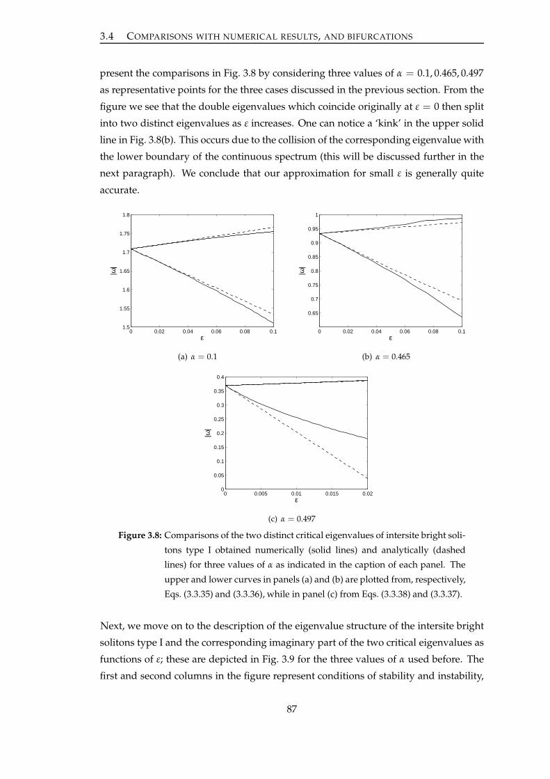
3.4 COMPARISONS WITH NUMERICAL RESULTS, AND BIFURCATIONS
present the comparisons in Fig. 3.8 by considering three values of α = 0.1, 0.465, 0.497
as representative points for the three cases discussed in the previous section. From the
figure we see that the double eigenvalues which coincide originally at ε = 0 then split
into two distinct eigenvalues as ε increases. One can notice a ‘kink’ in the upper solid
line in Fig. 3.8(b). This occurs due to the collision of the corresponding eigenvalue with
the lower boundary of the continuous spectrum (this will be discussed further in the
next paragraph). We conclude that our approximation for small ε is generally quite
accurate.
0 0.02 0.04 0.06 0.08 0.11.5
1.55
1.6
1.65
1.7
1.75
1.8
ε
|ω|
(a) α = 0.1
0 0.02 0.04 0.06 0.08 0.1
0.65
0.7
0.75
0.8
0.85
0.9
0.95
1
ε
|ω|
(b) α = 0.465
0 0.005 0.01 0.015 0.020
0.05
0.1
0.15
0.2
0.25
0.3
0.35
0.4
ε
|ω|
(c) α = 0.497
Figure 3.8: Comparisons of the two distinct critical eigenvalues of intersite bright soli-
tons type I obtained numerically (solid lines) and analytically (dashed
lines) for three values of α as indicated in the caption of each panel. The
upper and lower curves in panels (a) and (b) are plotted from, respectively,
Eqs. (3.3.35) and (3.3.36), while in panel (c) from Eqs. (3.3.38) and (3.3.37).
Next, we move on to the description of the eigenvalue structure of the intersite bright
solitons type I and the corresponding imaginary part of the two critical eigenvalues as
functions of ε; these are depicted in Fig. 3.9 for the three values of α used before. The
first and second columns in the figure represent conditions of stability and instability,
87

3.4 COMPARISONS WITH NUMERICAL RESULTS, AND BIFURCATIONS
respectively. For α = 0.1, the two critical eigenvalues successively collide with the
outer band of the continuous spectrum and the corresponding bifurcating eigenvalues
coming from the first collision contribute to the instability. For α = 0.465, the first
collision is between one of the critical eigenvalues with the inner edge of the continuous
spectrum. The second collision is between the other critical eigenvalue with its pair. In
contrast to the previous case, the instability in this case is caused by the bifurcating
eigenvalues coming from the second collision. Moreover, for α = 0.497, contribution
to the instability is given by one of the critical eigenvalues moving down along the
imaginary axis. All the numerical results described above are in accordance with our
analytical observations in Section 3.3.
Let us now focus our attention on the right panels of Fig. 3.9 by particularly discussing
the properties of the critical points of ε at which the curve of the minimum imaginary
part of the critical eigenvalues crosses the real axis (these are shown by the star mark-
ers). The first and third points (from left to right) in panel (c) as well as the points
in panels (f) and (i) indicate the onset of stable-to-unstable transition. Contrastingly,
the second point in panel (c) illustrates the beginning of the re-stabilisation of solitons.
In fact, the first three points in panel (c) mentioned above admit all conditions for the
occurrence of a Hopf bifurcation (see again the relevant explanation about these condi-
tions in our discussion of onsite type I); therefore, they also correspond to Hopf points.
In addition, the fourth point of zero crossing in panel (c), which comes from one of
the purely imaginary eigenvalues, indicates the branch point of a pitchfork bifurcation
experienced by the solutions of intersite type I, III and IV. We will discuss this type of
bifurcation in more detail in the next section.
The (in)stability region of intersite bright solitons type I in the (ε, α)-plane is given
in Fig. 3.10. In the figure, we also depict the two distinguishable (solid and dashed)
lines representing the two distinct critical eigenvalues whose imaginary parts become
zero. The star points on the lines correspond to those points in the right panels of
Fig. 3.9. The boundary line which separates the stable and unstable regions in the figure
is shown by the bold (solid and dashed) lines. The lower and upper dotted horizontal
lines in the figure represent, respectively, α = αcp ≈ 0.4583 and α = αth ≈ 0.49659
which divide the region into three different descriptions of the eigenvalue structure.
Interestingly, for αth < α, we can make an approximation for the numerically obtained
stability boundary (see the inset). This approximation is given by Eq. (3.3.39) which is
quite close to the numerics for small ε.
We notice in Fig. 3.10 that the solid line (not the rightmost) and dashed line also repre-
sent Hopf bifurcations, with one special point (the white-filled circle) which does not
88

3.4 COMPARISONS WITH NUMERICAL RESULTS, AND BIFURCATIONS
−2 −1 0 1 20
0.05
0.1
0.15
0.2
Re(ω)
Im(ω
)
(a) α = 0.1, ε = 0.08
−2 −1 0 1 2−0.05
0
0.05
0.1
0.15
0.2
Re(ω)Im
(ω)
(b) α = 0.1, ε = 0.35
0 0.2 0.4 0.6−0.1
0
0.1
0.2
0.3
ε
Im(ω
crit)
(c) α = 0.1
−1.5 −1 −0.5 0 0.5 1 1.50
0.2
0.4
0.6
0.8
Re(ω)
Im(ω
)
(d) α = 0.465, ε = 0.02
−1.5 −1 −0.5 0 0.5 1 1.5−1
−0.5
0
0.5
1
1.5
2
Re(ω)
Im(ω
)
(e) α = 0.465, ε = 0.5
0 0.2 0.4 0.6
0
0.2
0.4
0.6
0.8
1
εIm
(ωcr
it)(f) α = 0.465
−2 −1 0 1 20
0.2
0.4
0.6
0.8
1
Re(ω)
Im(ω
)
(g) α = 0.497, ε = 0.04
−2 −1 0 1 2−1
−0.5
0
0.5
1
1.5
2
Re(ω)
Im(ω
)
(h) α = 0.497, ε = 0.3
0 0.2 0.4 0.6
0
0.2
0.4
0.6
0.8
1
ε
Im(ω
crit)
(i) α = 0.497
Figure 3.9: The first and second columns of panels show the structure of eigenvalues
of intersite bright solitons type I in the complex plane, for three values of α,
each of which uses two different values of ε, to depict the condition of sta-
bility (left panel) and instability (middle panel). The third column shows
the imaginary part of the two distinct critical eigenvalues (presented by
solid and dashed lines) as functions of ε for the corresponding α. The loca-
tions of zero-crossings in these panels are indicated by the star markers.
89

3.4 COMPARISONS WITH NUMERICAL RESULTS, AND BIFURCATIONS
meet the second condition for the occurrence of a (non-degenerate) Hopf bifurcation
mentioned above (we will analyse the special point in the next section). We see from
the figure that the bold parts of the Hopf lines coincide with the (in)stability boundary,
while the nonbold ones exist in the unstable region. In addition, we also observe that
the rightmost solid line in Fig. 3.10 indicates the collection of branch points of pitchfork
bifurcation experienced by the intersite type I, III and IV; the bold part of this line also
indicates the (in)stability boundary.
ε
α
0 0.1 0.2 0.3 0.4 0.5 0.6 0.70
0.05
0.1
0.15
0.2
0.25
0.3
0.35
0.4
0.45
0.5
0 0.05 0.10.495
0.5
−1.4
−1.2
−1
−0.8
−0.6
−0.4
−0.2
0
0.2
0.4
stable
unstable
unstable unstable
Figure 3.10: As Fig. 3.4 but for intersite bright solitons type I. The boundary between
stable and unstable regions is given by the bold (solid and dashed) lines.
The dashed-dotted line in the inset is our analytical approximation given
by Eq. (3.3.39). The Hopf bifurcation lines are depicted by the solid (not
the rightmost) and dashed lines. The white-filled circle indicates a degen-
erate Hopf point. The branch points of pitchfork bifurcation are shown
by the rightmost solid lines.
3.4.2.2 Intersite type II
For intersite bright solitons type II, we present in Fig. 3.11 a comparison of two critical
eigenvalues between the numerics and the analytical calculation given by Eqs. (3.3.40)
and (3.3.41). We see from the figure that our approximation for relatively small ε is
quite close to the numerics. The snapshot of the eigenvalue structure of this type of
solution for two points (α, ε) and the path of the imaginary part of corresponding two
discrete eigenvalues are depicted in Fig. 3.12. We conclude that the intersite soliton
type II is unstable even for large ε.
Moreover, the evaluation of the minimum value of Im(ω) of the intersite bright solitons
90

3.4 COMPARISONS WITH NUMERICAL RESULTS, AND BIFURCATIONS
0 0.005 0.01 0.015 0.020.72
0.725
0.73
0.735
0.74
0.745
0.75
ε
|ω|
Figure 3.11: Comparison of two critical eigenvalues of intersite bright solitons type II
for α = 0.3 between numerics (solid lines) and analytics (dashed lines).
The analytical approximation is given by Eq. (3.3.40) (lower curve) and
Eq. (3.3.41) (upper curve).
type II in the (ε, α)-plane shows that the soliton, except at the point α = γ = 0.5 and
ε = 0, is always unstable. This result agrees with our analytical prediction.
3.4.2.3 Intersite type III and IV
Now we examine the intersite bright soliton type III which, due to symmetry, has ex-
actly the same eigenvalues as type IV. In Fig. 3.13, we plot the analytical approximation
for two critical eigenvalues given by Eqs. (3.3.42)-(3.3.43) or (3.3.44)-(3.3.45), which are
compared with the corresponding numerical results. We conclude that the approxima-
tion is quite accurate for small ε and that the range of accuracy is wider for smaller
value of α.
The structure of the eigenvalues of this type of solution and the curves of the imag-
inary part of the corresponding two critical eigenvalues are given in Fig. 3.14 for the
three values of α used in Fig. 3.13. The figure reveals the condition of instability of
solitons up to the limit points of ε at which the minimum imaginary part of the eigen-
values becomes zero; these conditions are indicated by the corresponding vertical lines
in the third column. In fact, these limit points indicate the branch points of pitchfork
bifurcation experienced by the intersite solitons type I, III and IV (we will discuss this
bifurcation in more detail in the next section).
The first and second columns of Fig. 3.14 respectively present the condition just be-
91

3.4 COMPARISONS WITH NUMERICAL RESULTS, AND BIFURCATIONS
−1.5 −1 −0.5 0 0.5 1 1.5−1
−0.5
0
0.5
1
1.5
Re(ω)
Im(ω
)
(a) α = 0.3, ε = 0.1
−1.5 −1 −0.5 0 0.5 1 1.5−1.5
−1
−0.5
0
0.5
1
1.5
2
Re(ω)
Im(ω
)
(b) α = 0.3, ε = 2
0 0.5 1 1.5 2 2.5
−1
−0.5
0
0.5
1
1.5
ε
Im(ω
crit)
(c) α = 0.3
Figure 3.12: (a)-(b) The eigenvalue structure of intersite bright solitons type II for two
values (α, ε) as indicated in the caption. (c) The imaginary part of two
discrete eigenvalues in varied ε (indicated by solid and dashed lines).
92

3.4 COMPARISONS WITH NUMERICAL RESULTS, AND BIFURCATIONS
0 0.005 0.01 0.015 0.02 0.025 0.030.8
0.9
1
1.1
1.2
1.3
1.4
1.5
1.6
1.7
1.8
ε
|ω|
(a) α = 0.1
0 0.002 0.004 0.006 0.008 0.010.4
0.5
0.6
0.7
0.8
0.9
1
ε|ω
|
(b) α = 0.465
0 0.2 0.4 0.6 0.8 1
x 10−3
0.2
0.25
0.3
0.35
0.4
ε
|ω|
(c) α = 0.497
Figure 3.13: Comparisons between two critical eigenvalues of intersite bright solitons
III and IV obtained numerically (solid lines) and analytically (dashed
lines) for values of α as shown in the caption. In panels (a) and (b), the up-
per and lower dashed curves correspond, respectively, to Eqs. (3.3.42) and
(3.3.43), whereas in panel (c) they correspond to Eqs. (3.3.44) and (3.3.45).
93

3.4 COMPARISONS WITH NUMERICAL RESULTS, AND BIFURCATIONS
fore and after a collision of one of the discrete eigenvalues which does not contribute
to the instability of solitons. Interestingly, as shown in panel (c), such an eigenvalue
also crosses the real axis at some critical ε as indicated by the empty circle. The lat-
ter condition, in fact, indicates a Hopf bifurcation, which occurs when the soliton is
already in unstable mode. This is different from the previous discussions where the
Hopf bifurcations also indicate the change of stability of solitons.
−2 −1 0 1 2−1.5
−1
−0.5
0
0.5
1
1.5
Re(ω)
Im(ω
)
(a) α = 0.1, ε = 0.1
−2 −1 0 1 2
−0.5
0
0.5
1
Re(ω)
Im(ω
)
(b) α = 0.1, ε = 0.5
0 0.2 0.4 0.6
−1
−0.5
0
0.5
1
ε
Im(ω
crit)
(c) α = 0.1
−1 −0.5 0 0.5 1−0.5
0
0.5
1
1.5
Re(ω)
Im(ω
)
(d) α = 0.465, ε = 0.01
−1 −0.5 0 0.5 1−0.5
0
0.5
1
1.5
Re(ω)
Im(ω
)
(e) α = 0.465, ε = 0.15
0 0.05 0.1 0.15 0.2−0.5
0
0.5
1
ε
Im(ω
crit)
(f) α = 0.465
−1 −0.5 0 0.5 1−0.2
0
0.2
0.4
0.6
0.8
1
1.2
Re(ω)
Im(ω
)
(g) α = 0.497, ε = 0.005
−1 −0.5 0 0.5 1−0.2
0
0.2
0.4
0.6
0.8
1
1.2
Re(ω)
Im(ω
)
(h) α = 0.497, ε = 0.04
0 0.02 0.04 0.06−0.2
0
0.2
0.4
0.6
0.8
1
ε
Im(ω
crit)
(i) α = 0.497
Figure 3.14: (First and second columns) The structure of eigenvalues of intersite bright
solitons type III and IV for parameter values (α, ε) as indicated in the
caption. (Third column) The imaginary part of two critical eigenvalues
(shown by solid and dashed lines) obtained by varying ε. The vertical
lines indicate the limit points of ε up to which the soliton exists, i.e., when
the minimum imaginary part of the eigenvalues becomes zero.
In Fig. 3.15 we present the (in)stability window for intersite bright solitons type III and
IV which is defined as the area to the left of the solid line; this line represents the set
of the branch points of pitchfork bifurcation in the (ε, α)-plane. From the figure, we
conclude that the intersite type III and IV are always unstable. The area to the right of
94

3.4 COMPARISONS WITH NUMERICAL RESULTS, AND BIFURCATIONS
the solid line belongs to the unstable region of intersite type I. One can check that this
line is exactly the same as the rightmost solid line in Fig. 3.10. In addition, the dashed
line appearing in Fig. 3.15 depicts the occurrence of Hopf bifurcations. However, there
is one special point indicated by the white-filled circle, at which the ε-derivative of
the imaginary part of the corresponding critical eigenvalue is zero; this degenerate
point will be discussed further in Section 3.5. The empty circle lying on the Hopf line
reconfirms the corresponding point in panel (c) of Fig. 3.14.
ε
α
0 0.1 0.2 0.3 0.4 0.5 0.6 0.70
0.05
0.1
0.15
0.2
0.25
0.3
0.35
0.4
0.45
0.5
−1.4
−1.2
−1
−0.8
−0.6
−0.4
−0.2
0
Intersite type II(unstable)
Intersite type III and IV(unstable)
Figure 3.15: The (in)stability region of intersite bright solitons type III and IV in (ε, α)-
space. The solid line indicates the branch-point line of pitchfork bifur-
cation. The dashed line represents the occurrence of Hopf bifurcations
(with one degenerate point at the white-filled circle), which arises from
one of the critical eigenvalues which does not contribute to the instability
of solitons. The empty circle lying on the dashed line corresponds to that
point depicted in panel (c) of Fig. 3.14.
3.4.2.4 Saddle-node and pitchfork bifurcation of intersite bright solitons
From both numerical and analytical results discussed above, we observed that the in-
tersite type I and II have the same profile and stability when approaching α = γ. This
fact indicates the appearance of a saddle-node bifurcation undergone by the two soli-
tons. Moreover, there also exists a pitchfork bifurcation experienced by the intersite
type I, III and IV.
One can check that the norm of the intersite type III and IV is exactly the same for
all parameter values so that this quantity can no longer be used for depicting a clear
bifurcation diagram. Therefore, we now simply plot the value of |u0|2 for each solution,
95

3.4 COMPARISONS WITH NUMERICAL RESULTS, AND BIFURCATIONS
e.g., as a function of α and fixed ε = 0.1; this is shown in Fig. 3.16 where the numerics
(solid lines) is obtained by a pseudo-arc-length method. As seen in the figure, the
intersite type I, III and IV meet at a (pitchfork) branch point (BP) α ≈ 0.49. At this point,
the stability of the intersite type I is switched. Furthermore, the intersite type I and II
also experience a saddle-node bifurcation where they merge at a limit point (LP) α =
γ = 0.5. Just before this point, the intersite type I possesses one unstable eigenvalue,
while the type II has two unstable eigenvalues. The two critical eigenvalues for the
intersite type I and II then coincide at LP. We confirm that our analytical approximation
for the value of |u0|2 is relatively close to the corresponding numerical counterpart.
Next, let us plot the value of |u0|2 for each soliton by fixing α = 0.1 and varying ε
(presented in Fig. 3.17). The pitchfork bifurcation experienced by the intersite type
I (solid line), type III (upper dashed line) and type IV (lower dashed line) is clearly
shown in the figure. The three solitons meet together at a branch point BP. We also
depict in the figure the points at which Hopf bifurcations emerge (labelled by indexed
H). For the shake of completeness, we also plot the relevant curve for the intersite type
II (dotted line).
0 0.1 0.2 0.3 0.4 0.5 0.6
0.4
0.6
0.8
1
1.2
1.4
1.6
1.8
2
α
|u0|2
−5 0 5
00.5
11.5
α=0.1
−5 0 5−1
0
1
α=0.1
−5 0 5−1
−0.5
0
α=0.1
−5 0 5−1
0
1
α = 0.1
−5 0 5−1
0
1
α = 0.5
−5 0 5−1
0
1
α ≈ 0.49
intersite type IV(unstable)
intersite type II (unstable)
intersite type III(unstable)
intersite type I (stable)
BP
LP
intersite type I (unstable)
Figure 3.16: Saddle-node and pitchfork bifurcations of intersite bright solitons by
varying α and fixing ε = 0.1. The curves depict the value of |u0|2 of
each solutions obtained numerically (solid lines) and analytically (dashed
lines). The profiles of the corresponding solutions at some values of α are
shown in the relevant insets. The intersite type I, III and IV merge at a
branch point (BP) α ≈ 0.49 and the intersite type I and II meet at a limit
point (LP) α = γ = 0.5.
96

3.5 NATURE OF HOPF BIFURCATIONS AND CONTINUATION OF LIMIT CYCLES
0 0.1 0.2 0.3 0.4 0.5 0.6 0.70.4
0.6
0.8
1
1.2
1.4
1.6
1.8
2
2.2
ε
|u0|2
BPH
2
H3
H1
H4
H5
Figure 3.17: A pitchfork bifurcation of intersite bright solitons for fixed α = 0.1 and
varied ε. The curves represent the numerical value of |u0|2 for the corre-
sponding solutions as a function of ε. The intersite type I (solid line), type
III (upper dashed line) and type IV (lower dashed line) merge at a branch
point (BP). The occurrence of Hopf bifurcation (Hi) is detected in intersite
type I, III and IV. The dotted line corresponds to the intersite type II.
3.5 Nature of Hopf bifurcations and continuation of limit cy-
cles
If there is only one pair of non-zero real eigenvalues and the other eigenvalues have
strictly positive imaginary parts, a Hopf bifurcation also indicates the change of sta-
bility of the steady state solution. In this case, the periodic solutions bifurcating from
the Hopf point coexist with either the stable or unstable mode of the steady state solu-
tion. If the periodic solutions coexist with the unstable steady state solution, they are
stable and the Hopf bifurcation is called supercritical. On the other hand, if the periodic
solutions coexist with the stable steady state solution, they are unstable and the Hopf
bifurcation is called subcritical.
By applying, for example, the centre manifold theorem, we can generally determine
the nature of a Hopf point εc through its first Lyapunov coefficient l1(εc) (see, e.g.,
Kuznetsov [115]); the Hopf bifurcation is subcritical iff l1(εc) > 0 and supercritical iff
l1(εc) < 0.
To numerically calculate the first Lyapunov coefficient for a Hopf point and perform a
continuation of the bifurcating limit cycle, we use the numerical continuation package
Matcont. Due to the limitations of Matcont, we evaluate the soliton using 21 sites. In
fact, this setting does not affect significantly the soliton behaviour compared to that
97

3.5 NATURE OF HOPF BIFURCATIONS AND CONTINUATION OF LIMIT CYCLES
used in the previous section.
In this section, we examine the nature of Hopf points and the stability of cycle contin-
uations in onsite type I, intersite type I and intersite type III-IV.
3.5.1 Onsite type I
For this type of solution, in particular at α = 0.1, we have one Hopf point, which oc-
curs at εc ≈ 0.3077 (see again panel (c) in Fig. 3.3). From Matcont, we obtain l1(εc ≈0.3077) > 0 which indicates that the Hopf point εc is subcritical and hence the limit
cycle bifurcating from this point is unstable. A continuation of the corresponding limit
cycle is given in Fig. 3.18(a). As the Hopf point in this case also indicates the change
of stability of the stationary soliton, one can confirm that the bifurcating periodic soli-
tons are unstable because they coexist with the stable onsite type I; this agrees with the
computed first Lyapunov coefficient above (the instability will be clearly shown in the
next section when we numerically evaluate its dynamics). Interestingly, the continua-
tion of the limit cycle also experiences saddle-node and torus bifurcations, as indicated
by the points labelled LPC (limit point cycle) and NS (Neimark-Sacker), respectively.
The profile of a representative periodic soliton over one period is shown in Fig. 3.18(b),
from which we clearly see the typical oscillation in the soliton amplitude.
0.25 0.26 0.27 0.28 0.29 0.3 0.31 0.321.1
1.2
1.3
1.4
1.5
1.6
1.7
1.8
1.9
ε
max
(||u
n||), m
in(|
|un||)
H
LPCNS
(a)
−10−5
05
10
0
1.7160
3.43190
0.5
1
1.5
nt
|un|
(b)
Figure 3.18: (a) The continuation of the limit cycle from a Hopf point H for an onsite
soliton type I with α = 0.1. The first Lyapunov coefficient for H cal-
culated by Matcont is positive, i.e., H is subcritical. The bold solid line
represents the norm of the stationary soliton while the solid and dashed
lines indicate, respectively, the maximum and minimum of the norm of
the bifurcating periodic solitons. (b) The profile of a periodic soliton over
one period (T ≈ 3.4319) corresponding to the black-filled circle in panel
(a).
98

3.5 NATURE OF HOPF BIFURCATIONS AND CONTINUATION OF LIMIT CYCLES
From the previous discussion we have mentioned that there is one degenerate point
for Hopf bifurcations in onsite type I, which is indicated by the white-filled circle in
Fig. 3.4. In Fig. 3.19, we depict numerical continuations of periodic orbits of two Hopf
bifurcations near the degenerate point. We obtained that the limit cycle branches bi-
furcating from the Hopf points are connected and form a closed loop. This informs us
that as α approaches the critical value for a degenerate Hopf point, the “radius” of the
loop tends to zero. Hence, one may conclude that at the double-Hopf point, there is no
bifurcation of periodic orbits.
1.45 1.455 1.46 1.465 1.47
2.054
2.056
2.058
2.06
2.062
2.064
ε
max
(||u
n||), m
in(|
|un||)
Figure 3.19: As Fig. 3.18(a) but for α = 0.492642. Two Hopf points (stars) in the neigh-
bourhood of the degenerate point (the while-filled circle in Fig. 3.4) are
shown to be connected by a branch of limit cycles.
3.5.2 Intersite type I
In particular for α = 0.1, there are three Hopf points detected for the intersite type I (see
again Fig. 3.17). For point H1 (εc ≈ 0.2782), Matcont gives a negative value for the first
Lyapunov coefficient, which means that the bifurcating periodic soliton is stable or H1
is supercritical (we confirm the stability in the next section by examining its numerical
evolution). The corresponding cycle continuation is presented in Fig. 3.20(a). As shown
in the figure, the limit cycle bifurcating from H1 coexist with the unstable mode of the
(steady-state) intersite type I which confirms the supercritical H1 (recall that the Hopf
bifurcation in this case also indicates the change of stability of the soliton, i.e., it is
stable (unstable) just below (above) εc ≈ 0.2782 [see again Fig. 3.9(c)]). We also see
from the figure that the cycle continuation contains NS, LPC and BPC (branch point
cycle) points which indicate the occurrence of, respectively, torus, saddle-node and
99
3.5 NATURE OF HOPF BIFURCATIONS AND CONTINUATION OF LIMIT CYCLES
pitchfork bifurcations for limit cycle. The branches of the cycle continuation from the
BPC point are shown in the figure. A representative periodic soliton (in one period)
which occurs at one representative point along the cycle continuation is depicted in
Fig. 3.20(b), which shows the oscillation between the two excited sites.
Next, for H2 (εc ≈ 0.3871) and H3 (εc ≈ 0.4934), the first Lyapunov coefficients given by
Matcont are negative and positive valued, respectively. Thus, H2 is supercritical while
H3 is subcritical, which implies that the limit cycles bifurcating from H2 and H3 are
stable and unstable, respectively (confirmation of these stability findings through their
numerical dynamics will be shown in the next section). The continuations of the corre-
sponding limit cycles are shown in Fig. 3.21(a). From the figure, we see that the limit
cycles bifurcating from H2 and H3 respectively coexist with the unstable and stable sta-
tionary intersite soliton type I. This fact is consistent with the nature of H2 and H3 as
given by Matcont. In addition, as shown in the figure, a period-doubling (PD) bifur-
cation also occurs in the cycle continuation coming from H3. This bifurcation seems to
coincide with the turning point of cycle (LPC) which appears in the cycle continuation
starting from H2. The profile of one-period periodic solitons at the two representative
points near H2 and H3 are presented in Figs. 3.21(b) and 3.21(c), respectively. We can-
not see clearly the typical oscillation of the periodic soliton shown in the upper panel of
Fig. 3.21(b) as it occurs very near to H2. However by plotting the absolute value of the
solution at site n = 0 and n = 1 over one period (see the lower panel of Fig. 3.21(b)), one
can confirm the oscillation between the two excited sites. By contrast, the oscillation in
the soliton amplitude is clearly visible in Fig. 3.21(c).
Similarly to the onsite type I, we also noticed the presence of a double-Hopf bifurcation
in the intersite type I, i.e., the white-filled circle in Fig. 3.10. To investigate the point,
we evaluate several Hopf points nearby the bifurcation point and perform numerical
continuations for limit cycles, which are presented in Fig. 3.22. Unlike the case in the
onsite type I, here the (non-degenerate) Hopf points are not connected to each other by
a closed loop of a branch of limit cycles. As we observe this scenario at any Hopf point
that is arbitrarily close (up to a numerical accuracy) to the degenerate (codimension 2)
bifurcation, it indicates that at the double-Hopf point, there is a bifurcation of at least
two branches of periodic solutions.
3.5.3 Intersite type III and IV
As intersite bright soliton type III and IV possess the same eigenvalue structures, the
nature of the corresponding Hopf bifurcation and the stability of the continuation of
each limit cycle will be the same as well. Therefore it is sufficient to devote our discus-
100

3.5 NATURE OF HOPF BIFURCATIONS AND CONTINUATION OF LIMIT CYCLES
0.25 0.26 0.27 0.28 0.29
1
1.5
2
2.5
3
ε
max
(|u 0|2 ),
min
(|u 0|2 )
LPCBPCNS
LPCBPCNS
H1
(a)
−10−5
05
10
0
2.7633
5.52650
0.5
1
1.5
nt
|un|
(b)
0.27 0.271 0.272 0.273 0.274 0.275 0.276
2.46
2.48
2.5
2.52
2.54
2.56
2.58
2.6
2.62
2.64
ε
max
(|u 0|2 ),
min
(|u 0|2 )
LPCBPCNS
(c)
0.272 0.274 0.276 0.278 0.28
1.05
1.1
1.15
1.2
1.25
1.3
1.35
ε
max
(|u 0|2 ),
min
(|u 0|2 )
LPCBPCNS
(d)
Figure 3.20: (a) The cycle continuation from Hopf point H1 for intersite bright soliton
type I with α = 0.1. In this case, H1 is supercritical. The bold solid line
indicates the value of |u0|2 for the stationary soliton, which is the same
as that shown in Fig. 3.17. The solid and dashed lines represent, respec-
tively, the maximum and minimum value of |u0|2 for the bifurcating pe-
riodic solitons, which also experience a pitchfork cycle bifurcation. The
branches of the cycle are depicted by the dash-dotted (maximum |u0|2)
and dotted (minimum |u0|2) lines. (b) The profile of a periodic soliton
over one period (T ≈ 5.5265) corresponding to the star point in panel (a).
(c,d) Enlargements of, respectively, the upper and the lower rectangles in
panel (a).
.
101

3.5 NATURE OF HOPF BIFURCATIONS AND CONTINUATION OF LIMIT CYCLES
0.38 0.4 0.42 0.44 0.46 0.48 0.5
1.4
1.6
1.8
2
2.2
2.4
2.6
LPC
LPC
ε
max
(|u 0|2 ),
min
(|u 0|2 )
PD
PD
0.387 0.3872
1.78
1.8
1.82
1.84LPCPDNS
H3
H2
H2
(a)
−10 −5 05 10
0 3.354
6.7080
0.5
1
1.5
nt
|un|
0 3.354 6.7081.34
1.3451.35
t
|u0|,|
u 1|
|u
0|
|u1|
(b)
−10−5
05
10
0
1.7493
3.49850
0.5
1
1.5
nt
|un|
(c)
Figure 3.21: (a) As Fig. 3.20(a) but for H2 and H3, where the inset gives the zoom-in
for the corresponding region showing that H2 and H3 are supercritical
and subcritical, respectively. The bold solid line is the same as that shown
in Fig. 3.17, i.e., representing the value of |u0|2 for the stationary intersite
soliton. The solid (dashed) and dash-dotted (dotted) lines shows the max-
imum (minimum) value of |u0|2 for the periodic soliton which bifurcates
from, respectively, H2 and H3. (b,c) The profile of periodic solitons over
one period T ≈ 6.708 and T ≈ 3.4985 which corresponds, respectively, to
the star and the black-filled circle in panel (a).
102

3.5 NATURE OF HOPF BIFURCATIONS AND CONTINUATION OF LIMIT CYCLES
0.33 0.34 0.35 0.36 0.371.5
1.6
1.7
1.8
1.9
2
2.1
2.2
ε
max
(|u 0|2 ),
min
(|u 0|2 )
LPC
LPC
LPC
LPC
LPC
LPC
Figure 3.22: As Fig. 3.21(a) but for α = 0.108 (triangles) and α = 0.11082 (stars) in the
proximity of the while-filled circle in Fig. 3.10.
sion to intersite type III only.
As shown in Fig. 3.17, there is one Hopf point, namely H4, for the intersite type III at
α = 0.1. In this type of solution, the Hopf bifurcation occurs while other eigenvalues
already give rise to instability; this is different from the type of Hopf bifurcation dis-
cussed previously. Therefore we cannot perform the analysis as before in determining
the stability of the bifurcating periodic soliton. In fact, according to calculation given
by Matcont, the first Lyapunov coefficient for H4 is positive (subcritical), which means
that the bifurcating periodic soliton is unstable. As shown in the next section, this
instability will be confirmed through its time evolution.
Fig. 3.23(a) shows the continuation of the corresponding limit cycle from H4. A repre-
sentative one-period periodic soliton at ε near H4 (indicated by the black-filled circle)
is shown in Fig. 3.23(b), from which we can see clearly the oscillation in the amplitude
of soliton.
Next, we study the double-Hopf bifurcation for the intersite type III-IV shown by the
white-filled circle in Fig. 3.15. We present in Fig. 3.24 the continuation of the limit
cycles from two Hopf points about the degenerate point, from which we see that they
are connected to each other. Therefore, as for the case of the onsite type I, we argue that
there is no bifurcation of periodic solutions at the degenerate point.
103

3.5 NATURE OF HOPF BIFURCATIONS AND CONTINUATION OF LIMIT CYCLES
0.32 0.34 0.36 0.38 0.4
1
1.5
2
2.5
3
H4
ε
max
(|u 0|2 ),
min
(|u 0|2 )
LPC
LPC
LPC
LPC
(a)
−10−5
05
10
0
1.8694
3.73880
0.5
1
1.5
nt
|un|
(b)
Figure 3.23: (a) The cycle continuation from Hopf point H4 for intersite bright soliton
type III with α = 0.1 showing that H4 is subcritical. The dashed line
shows the value of |u0|2 for the stationary soliton (the same as that shown
in Fig. 3.17) while the solid and dotted lines represent, respectively, the
maximum and minimum |u0|2 of the bifurcating periodic solitons. (b) The
profile of a periodic soliton over one period T ≈ 3.7388 corresponding to
the black-filled circle in panel (a).
0.486 0.488 0.49 0.492 0.494 0.496 0.4981.85
1.9
1.95
2
2.05
2.1
2.15
ε
max
(|u 0|2 ),
min
(|u 0|2 )
Figure 3.24: As Fig. 3.23(a) but for α = 0.1411. The degenerate (Hopf-Hopf) point
indicated as the while-filled circle in Fig. 3.15 is at ε ≈ 0.49.
104

3.6 NUMERICAL INTEGRATIONS
3.6 Numerical integrations
In this section, we confirm our stability findings through integrating numerically the
time-dependent equation (3.1.1). To do so, we use a fourth-order Runge-Kutta method
with the initial condition being the corresponding stationary soliton solution of equa-
tion (3.2.1). The numerical integration of Eq. (3.1.1) is also examined to confirm the
stability findings for the bifurcating periodic solutions as discussed above.
3.6.1 Stationary solitons
Here we particularly examine the dynamics of the stationary solitons of which the
initial profiles correspond to the eigenvalue structures depicted in the figures of Sec-
tion 3.4. We show that the dynamics of the stable and unstable solitons are consistent
with, respectively, the stability and instability mode of the corresponding eigenvalue
structures.
We begin by evaluating the onsite soliton type I. The numerical evolution of this type
of soliton is shown in Fig. 3.25. In the top right panel, the typical dynamics of the
unstable soliton is in the form of oscillatory instability which decays and then vanishes
completely. In contrast, the unstable soliton in the middle right panel evolves to a
seemingly stable oscillatory solution.
In Fig. 3.26 we present the dynamics of the onsite soliton type II which was observed
previously as being always unstable, except at α = γ (note that the linearised Eq. (3.1.1)
has solutions of the form e(γ−α)t, thus the stability of soliton when α = γ is basically
due to a balance between damping and driving parameters). As shown in the left panel,
the unstable soliton manifests itself in the form of oscillation in the centre of the soliton
with different frequency and amplitude, which then becomes constant. Contrastingly,
the typical instability of the unstable soliton in the right panel is in the form of soliton
decay, which leads to the zero solution just after a short period of time.
Next, we examine the dynamics of the intersite bright soliton type I, which is illustrated
in Fig. 3.27. In the middle and bottom right panels, we see that the unstable intersite
soliton changes into an onsite soliton. By contrast, the unstable intersite soliton in the
top right panel still preserves its two-excited-state nature but suddenly shifts to the
next sites with different amplitude.
For intersite bright soliton type II, which was shown to be always unstable except at
the point α = γ = 0.5 and ε = 0, we present its time dynamics in Fig. 3.28 for two
representative unstable solitons. As we see from the figure, the instability makes the
105
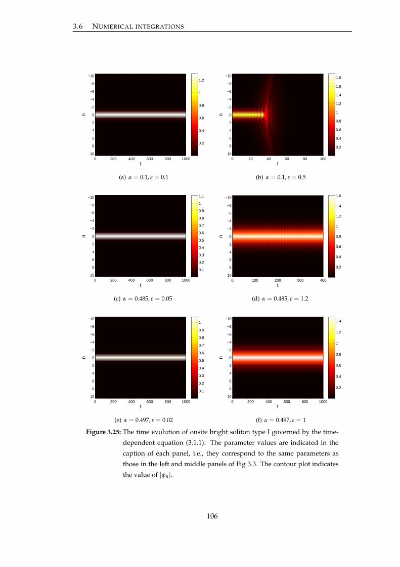
3.6 NUMERICAL INTEGRATIONS
t
n
0 200 400 600 800 1000
−10
−8
−6
−4
−2
0
2
4
6
8
10
0.2
0.4
0.6
0.8
1
1.2
(a) α = 0.1, ε = 0.1
t
n
0 20 40 60 80 100
−10
−8
−6
−4
−2
0
2
4
6
8
10
0.2
0.4
0.6
0.8
1
1.2
1.4
1.6
1.8
(b) α = 0.1, ε = 0.5
t
n
0 200 400 600 800 1000
−10
−8
−6
−4
−2
0
2
4
6
8
100.1
0.2
0.3
0.4
0.5
0.6
0.7
0.8
0.9
1
1.1
(c) α = 0.485, ε = 0.05
t
n
0 100 200 300 400
−10
−8
−6
−4
−2
0
2
4
6
8
10
0.2
0.4
0.6
0.8
1
1.2
1.4
1.6
(d) α = 0.485, ε = 1.2
t
n
0 200 400 600 800 1000
−10
−8
−6
−4
−2
0
2
4
6
8
10
0.1
0.2
0.3
0.4
0.5
0.6
0.7
0.8
0.9
1
(e) α = 0.497, ε = 0.02
t
n
0 200 400 600 800 1000
−10
−8
−6
−4
−2
0
2
4
6
8
10
0.2
0.4
0.6
0.8
1
1.2
1.4
(f) α = 0.497, ε = 1
Figure 3.25: The time evolution of onsite bright soliton type I governed by the time-
dependent equation (3.1.1). The parameter values are indicated in the
caption of each panel, i.e., they correspond to the same parameters as
those in the left and middle panels of Fig 3.3. The contour plot indicates
the value of |φn|.
106

3.7 CONCLUSION
t
n
0 10 20 30 40 50
−10
−8
−6
−4
−2
0
2
4
6
8
10
0.2
0.4
0.6
0.8
1
1.2
1.4
(a) α = 0.1, ε = 0.01
t
n
0 5 10 15 20 25 30
−10
−8
−6
−4
−2
0
2
4
6
8
100.2
0.4
0.6
0.8
1
1.2
1.4
1.6
1.8
2
2.2
(b) α = 0.1, ε = 1
Figure 3.26: As Fig. 3.25, but for onsite type II. The eigenvalue structure of the initial
profile in each panel is shown in Fig. 3.6.
soliton change its profile into an onsite mode (left panel) or decay (right panel).
Finally, we present the numerical evolution of intersite soliton type III-IV in Fig. 3.29.
We have confirmed the instability of this soliton in the previous discussion. All the
typical dynamics of the unstable soliton presented in Fig. 3.29 are in the form of loss of
its asymmetry, i.e., each soliton turns into a symmetric intersite soliton just after a short
time.
3.6.2 Periodic solitons
In this section, we examine the dynamics of the time-dependent Eq. (3.1.1) for the pe-
riodic solitons which arise at the corresponding Hopf bifurcations experienced by the
onsite type I, intersite type I and intersite type III-IV. The time evolution of the peri-
odic solitons whose profiles were depicted in the corresponding figures in Section 3.5
is presented in Fig. 3.30. From the figure, we can confirm the relevance of the stability
of the periodic solitons investigated in Section 3.5. The typical dynamics of the unsta-
ble periodic solitons is in the form of breather destruction which eventually leads to
zero solution. For periodic intersite soliton type III and IV [panel (e)], this destruction
happens after just a short time.
3.7 Conclusion
In this chapter, we have considered a parametrically driven damped discrete nonlin-
ear Schrödinger (PDDNLS) equation. The existence and stability of fundamental dis-
crete bright solitons have been examined analytically through a perturbation theory for
107

3.7 CONCLUSION
t
n
0 200 400 600 800 1000
−10
−8
−6
−4
−2
0
2
4
6
8
10
0.2
0.4
0.6
0.8
1
1.2
(a) α = 0.1, ε = 0.08
t
n
0 200 400 600 800 1000
−10
−8
−6
−4
−2
0
2
4
6
8
10
0.2
0.4
0.6
0.8
1
1.2
1.4
1.6
1.8
2
(b) α = 0.1, ε = 0.35
t
n
0 200 400 600 800 1000
−10
−8
−6
−4
−2
0
2
4
6
8
100.1
0.2
0.3
0.4
0.5
0.6
0.7
0.8
0.9
1
1.1
(c) α = 0.465, ε = 0.02
t
n
0 20 40 60 80 100
−10
−8
−6
−4
−2
0
2
4
6
8
10
0.2
0.4
0.6
0.8
1
1.2
1.4
(d) α = 0.465, ε = 0.5
t
n
0 200 400 600 800 1000
−10
−8
−6
−4
−2
0
2
4
6
8
10
0.1
0.2
0.3
0.4
0.5
0.6
0.7
0.8
0.9
1
(e) α = 0.497, ε = 0.04
t
n
0 20 40 60 80 100
−10
−8
−6
−4
−2
0
2
4
6
8
10
0.2
0.4
0.6
0.8
1
1.2
(f) α = 0.497, ε = 0.3
Figure 3.27: As Fig. 3.25, but for intersite type I with the same parameter values as
those in the left and middle panels of Fig. 3.9.
108

3.7 CONCLUSION
t
n
0 20 40 60 80 100
−10
−8
−6
−4
−2
0
2
4
6
8
10
0.2
0.4
0.6
0.8
1
1.2
1.4
(a) α = 0.3, ε = 0.1
t
0 20 40 60 80 100
−10
−8
−6
−4
−2
0
2
4
6
8
100.2
0.4
0.6
0.8
1
1.2
1.4
1.6
1.8
2
2.2
(b) α = 0.3, ε = 2
Figure 3.28: As Fig. 3.25, but for intersite bright soliton type II. The initial profile
in each panel has the corresponding eigenvalue structure depicted in
Fig. 3.12.
small ε and then corroborated by numerical calculations. We showed that there are two
types of onsite discrete soliton, namely onsite type I and II. For onsite type I, we found
an interval in α for which the soliton is stable for any coupling constant, i.e., a damping
can re-stabilise a driven onsite soliton. Contrastingly, the onsite type II was found to be
always unstable for all ε. These two solitons experience a saddle-node bifurcation with
the limit point α = γ for any ε.
We also showed that there are four types of intersite discrete soliton, called intersite
type I, II, III and IV. In fact, intersite type III and IV are essentially considered as one
solution due to its symmetry. We obtained that intersite type I in the region of insta-
bility in the non-dissipative case can be stabilised by damping while intersite type II
and III-IV are always unstable. A saddle-node bifurcation, as for the onsite soliton,
was found to be undergone by intersite type I and II. Moreover, we also obtained that
intersite type I, III and IV experience a pitchfork bifurcation. The branch points of such
a bifurcation in the (ε, α)-plane have been calculated numerically.
More interestingly, we observed that Hopf bifurcation also occurs in onsite type I, in-
tersite type I and intersite type III-IV, which confirms the existence of the correspond-
ing periodic solitons (limit cycles) in the PDDNLS equation. The continuation of the
limit cycles as well as the stability of the periodic solitons have been demonstrated nu-
merically using the numerical continuation software Matcont. In particular, subcritical
Hopf bifurcations for onsite type I and intersite type III-IV were observed. Moreover,
we obtained three Hopf bifurcations for intersite type I. It was shown that two of these
points generate stable periodic solitons, i.e., the bifurcations are supercritical. The rel-
evance of the stability findings has been confirmed through numerical integrations of
109

3.7 CONCLUSION
t
n
0 20 40 60 80 100
−10
−8
−6
−4
−2
0
2
4
6
8
10
0.2
0.4
0.6
0.8
1
1.2
1.4
(a) α = 0.1, ε = 0.1
t
n
0 20 40 60 80 100
−10
−8
−6
−4
−2
0
2
4
6
8
10
0.2
0.4
0.6
0.8
1
1.2
1.4
(b) α = 0.1, ε = 0.5
t
n
0 20 40 60 80 100
−10
−8
−6
−4
−2
0
2
4
6
8
100.1
0.2
0.3
0.4
0.5
0.6
0.7
0.8
0.9
1
1.1
(c) α = 0.465, ε = 0.01
t
n
0 20 40 60 80 100
−10
−8
−6
−4
−2
0
2
4
6
8
100.1
0.2
0.3
0.4
0.5
0.6
0.7
0.8
0.9
1
1.1
(d) α = 0.465, ε = 0.15
t
n
0 20 40 60 80 100
−10
−8
−6
−4
−2
0
2
4
6
8
10
0.1
0.2
0.3
0.4
0.5
0.6
0.7
0.8
0.9
1
(e) α = 0.497, ε = 0.005
t
n
0 20 40 60 80 100
−10
−8
−6
−4
−2
0
2
4
6
8
10
0.1
0.2
0.3
0.4
0.5
0.6
0.7
0.8
0.9
1
(f) α = 0.497, ε = 0.04
Figure 3.29: As Fig. 3.25, but for intersite type III and IV. The dynamics of all unstable
solitons presented here corresponds to the unstable mode of the eigen-
value structures in Fig. 3.14.
110
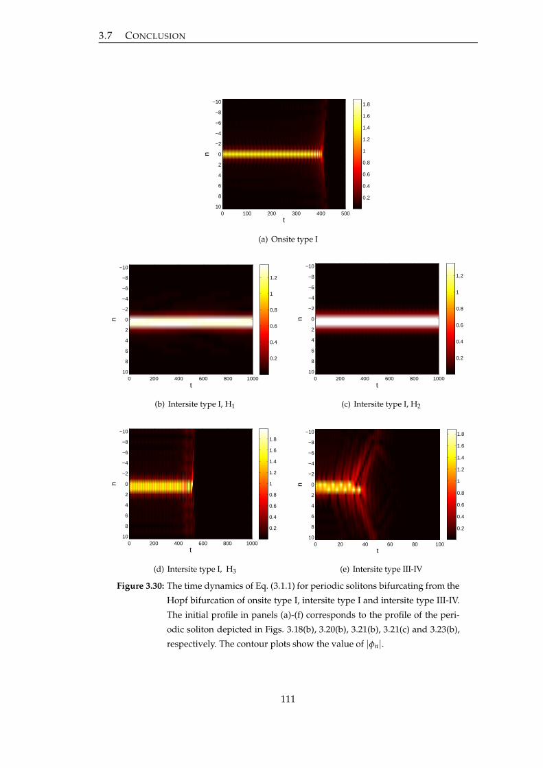
3.7 CONCLUSION
t
n
0 100 200 300 400 500
−10
−8
−6
−4
−2
0
2
4
6
8
10
0.2
0.4
0.6
0.8
1
1.2
1.4
1.6
1.8
(a) Onsite type I
t
n
0 200 400 600 800 1000
−10
−8
−6
−4
−2
0
2
4
6
8
10
0.2
0.4
0.6
0.8
1
1.2
(b) Intersite type I, H1
t
n
0 200 400 600 800 1000
−10
−8
−6
−4
−2
0
2
4
6
8
10
0.2
0.4
0.6
0.8
1
1.2
(c) Intersite type I, H2
t
n
0 200 400 600 800 1000
−10
−8
−6
−4
−2
0
2
4
6
8
10
0.2
0.4
0.6
0.8
1
1.2
1.4
1.6
1.8
(d) Intersite type I, H3
t
n
0 20 40 60 80 100
−10
−8
−6
−4
−2
0
2
4
6
8
10
0.2
0.4
0.6
0.8
1
1.2
1.4
1.6
1.8
(e) Intersite type III-IV
Figure 3.30: The time dynamics of Eq. (3.1.1) for periodic solitons bifurcating from the
Hopf bifurcation of onsite type I, intersite type I and intersite type III-IV.
The initial profile in panels (a)-(f) corresponds to the profile of the peri-
odic soliton depicted in Figs. 3.18(b), 3.20(b), 3.21(b), 3.21(c) and 3.23(b),
respectively. The contour plots show the value of |φn|.
111

3.7 CONCLUSION
the time-dependent PDDNLS equation for both stationary and periodic solitons.
112
CHAPTER 4
Travelling solitons in a discrete
nonlinear Schrödinger equation
with saturable nonlinearity
In the last two chapters, we have dealt with the discrete nonlinear Schrödinger (DNLS)
equation with cubic nonlinearity by introducing the effect of parametric driving and/or
damping. In this chapter, our study is devoted to another type of DNLS systems char-
acterised by the so-called saturable nonlinearity. While the study in Chapters 2 and 3
is particularly concerned with standing wave solutions, here we focus our attention on
travelling waves of the lattice system.
4.1 Introduction
One of the major issues in studies of spatially discrete systems is whether such systems
can support solitary waves that travel without losing energy to radiation, which results
in deceleration and eventually pinning of the solitons. The celebrated Peierls-Nabarro
(PN) barrier [63, 64] is the reason that discrete systems do not generically support ex-
ponentially localised travelling solitary waves. The barrier corresponds to the energy
difference between the onsite- and the intersite-centred lattice solitons, with the latter
usually having a higher energy.
The first attempt at finding travelling solitons in lattice system modelled by a discrete
nonlinear Schrödinger (DNLS) equation was undertaken by Eilbeck [116], followed
by a more systematic study by Feddersen [117] and Duncan et al. [118]. The latter
works indicate that travelling lattice solitons in the DNLS system are accompanied by
nonzero-radiation tails, which was confirmed by more recent studies (see, e.g., Gómez-
113

4.1 INTRODUCTION
Gardeñes et al. [68, 119], Melvin et al. [69] and Pelinovsky et al. [120]).
While the most typical onsite nonlinearity in DNLS models is cubic, waveguiding ar-
rays made of photorefractive materials feature the saturable nonlinearity. Under appro-
priate conditions, the saturable nonlinearity may be approximated by a truncated poly-
nomial nonlinearity, e.g., a cubic–quintic truncation. One- and two-dimensional (1D
and 2D) solitons in the DNLS with the cubic–quintic onsite nonlinearity have also been
studied in some detail (see, e.g., Carretero-González et al. [81] and Chong et al. [121]).
It was found that the saturable nonlinearity readily supports travelling solitons in
discrete media (Hadžievski et al. [65] and Vicencio & Johansson [122]). A reason for
this property is the fact that the PN barrier can change its sign in the case of the sat-
urable nonlinearity [65], hence the barrier may vanish at isolated points (see the rele-
vant discussion about this in Section 1.4.3). This property may be essential in finding
lattice solitary waves that can travel permanently without emitting radiation (lattice
phonons).
4.1.1 The considered model and preliminary analyses
The saturable DNLS equation modelling the propagation of optical waves in a photore-
fractive medium is
idφn
dt= −ε∆2φn(t)− Λφn(t) +
σφn(t)
1 + |φn(t)|2, (4.1.1)
where, as in the previous governing equations in Chapters 2 and 3, φn is a complex-
valued wave function at site n, ε is the strength of the coupling between adjacent sites,
∆2φn(t) = φn+1(t) − 2φn(t) + φn−1(t) is the 1D discrete Laplacian, Λ is a background
frequency and σ is the nonlinearity coefficient. We note that the transformation
t → t/σ, ε → σε, Λ → σΛ (4.1.2)
allows us to replace σ in Eq. (4.1.1), without loss of generality, by 1, implying that the
onsite nonlinearity is self-focusing provided that ε > 0.
To study travelling-wave solutions of Eq. (4.1.1), an ansatz of the form
φn(t) = ψ(z, τ), (4.1.3)
with z = n − ct and τ = t, is substituted into the equation to yield the time-dependent
advance–delay-differential equation
− icψz(z, τ) + iψτ(z, τ) = (2ε − Λ)ψ(z, τ)− ε [ψ(z + 1, τ) + ψ(z − 1, τ)]
+ψ(z, τ)
1 + |ψ(z, τ)|2 , (4.1.4)
114

4.1 INTRODUCTION
where c is the velocity. Travelling-wave solutions of Eq. (4.1.1) can be sought using the
time-independent version of Eq. (4.1.4),
− icψ′ = (2ε − Λ)ψ(z)− ε [ψ(z + 1) + ψ(z − 1)] +ψ(z)
1 + |ψ(z)|2 , (4.1.5)
with ψ′ ≡ dψdz .
Eq. (4.1.5) admits the existence of rotational and translational invariance under trans-
formations
ψ → ψeiθ, θ ∈ R, (4.1.6)
and
ψ(z) → ψ(z + z), z ∈ R, (4.1.7)
respectively. However, our attention is focused on the fundamental single hump soli-
ton solutions of Eq. (4.1.5). Therefore we will look for solutions that are invariant under
the reversing symmetry
z → −z, ψ → ψ∗, (4.1.8)
where the asterisk denotes complex conjugation. From this reversibility property, we
may construct a soliton solution whose real part is an even function whereas the imag-
inary part is odd, and thus ψ(0) is real.
4.1.2 Previous works on the saturable DNLS model
In the particular case of σ = Λ, exact stationary solutions of Eq. (4.1.1) including the
soliton solutions have been derived by Khare et al. [123, 124]. The stability of the ob-
tained solutions was also discussed therein, and the solutions were shown numerically
to be linearly stable in most cases. Moreover, the stationary onsite and intersite dark
solitons in the defocusing case of Eq. (4.1.1), i.e., when Λ < 0 and σ < 0, have also been
considered by Fitrakis et al. [86] by using an anticontinuum (AC) limit approach. In the
latter reference, it was shown that the onsite solutions are stable for small values of ε,
while the intersite solutions are always unstable.
The existence of travelling solitons for the saturable DNLS was investigated numer-
ically by Melvin et al. [66, 67] by solving Eq. (4.1.5) using a pseudo-spectral method,
which yielded weakly delocalised solitary waves, i.e., the solutions are accompanied
by nonzero oscillating tails. Genuinely localised pulse-like solutions were then gener-
ated by finding zeros of an appropriately defined measure of the tail amplitude. The
idea of identifying truly localised solutions from the “tail condition” is similar to that
used by Yang et al. [125]. In the later reference, the term embedded solitons (ESs) was in-
troduced for the first time for such solutions, which we will explain later. In Melvin et
115

4.1 INTRODUCTION
al. [66], the stability of the obtained solutions was analysed numerically by calculating
the Floquet multipliers of the solutions, using methods similar to that developed by
Gómez-Gardeñes et al. [119].
The presence of genuinely travelling lattice solitons in the saturable DNLS in the strong-
coupling case has been shown analytically by Oxtoby and Barashenkov, using expo-
nential asymptotic methods [126] (see also Melvin et al. [69]). The use of this sophisti-
cated technique is necessary, as the radiation emitted by moving solitary waves is expo-
nentially small in the wave’s amplitude. This is a reason why broad, small-amplitude
pulses in weakly coupled systems or lattice solitons in strongly coupled systems are
highly mobile, seeming like freely travelling solitons.
4.1.3 Overview
In this chapter, we revisit the study of the existence and stability of travelling solitary
waves in the saturable DNLS (4.1.1), which, as pointed out in the previous section, has
been discussed and solved numerically by Melvin et al. [66, 67]. Here we use a different
approach in both our numerical and analytical methods.
To examine the existence of the travelling solitary waves, following Melvin et al. [66,
67], first we need to solve the linear spectrum of Eq. (4.1.5); we perform this both nu-
merically and analytically using a perturbation expansion. The analysis leads us to
produce the diagram of the spectral bands from which we can identify the parameter
regions where a single resonance of the travelling solutions with plane waves occurs,
and thus finding isolated solutions with vanishing tails by varying one parameter only
within this regions becomes possible.
Next, to solve numerically Eq. (4.1.5) within the single-resonance parameter regions,
instead of using a pseudo spectral method as implemented by Melvin et al. [66, 67],
we propose an alternative scheme based on the discretization of Eq. (4.1.5). This dis-
cretization results in a system of difference equations which is then solved using a
Newton–Raphson method.
The numerically obtained soliton solutions in our scheme, as in Melvin et al. [66, 67], are
generally accompanied by oscillatory tails with a non-vanishing amplitude. Therefore,
to find solutions with non-oscillatory tails, as suggested in the latter references, we
need to add an extra tail condition. For this condition we consider either the measure
modified from that proposed by Melvin et al. [66, 67] or our alternative measure. All
of our numerical findings are then benchmarked against those in [66], confirming the
robustness of the results. However, we find that our numerical method is not accurate
116

4.2 DISPERSION RELATIONS
to examine the stability of solitons as the calculation of the corresponding eigenvalue
problem by means of our alternative scheme gives spurious unstable eigenvalues. This
is in contrast to the numerical results of [66], where the solitons were reported to be
linearly stable.
Moreover, we apply the variational approximation (VA) to study travelling solitary
waves and their stability analytically. The VA is also derived to predict the location
of ESs, i.e., the genuinely localised travelling solitary waves. The VA was applied to
construct fundamental discrete soliton solutions in the DNLS equation with cubic non-
linearity as well as in other variants of DNLS models (see Section 1.4.4.3 for a review
of the previous works which implemented the VA).
The chapter is organised as follows. In Section 4.2, we discuss the linear spectrum
of the advance–delay equation (4.1.5), and a perturbation expansion is performed to
obtain analytical approximations for the spectral bands. In Section 4.3, we introduce
our numerical scheme for solving Eq. (4.1.5) and then benchmark our results against
those obtained by Melvin et al. [66]. Next, in Section 4.4, we develop the VA for the
solitary-wave solutions of the advance-delay equation. In the same section, we derive
an analytical function whose zeros correspond to the location of ESs. The use of the VA
in analysing the stability of the travelling solitary waves is also discussed in the section.
In addition to saturable model, for comparison purposes, we also derived in Section 4.4
the similar variational formulations for a polynomial DNLS equation. Comparisons
of our findings obtained from the VA with the corresponding numerical results are
then presented in Section 4.5. Moreover, we address in Section 4.6 the failure of our
numerical scheme in examining the stability of the solitons. Finally, we summarise our
results in Section 4.7.
4.2 Dispersion relations
As discussed by Melvin et al. [66, 67], travelling solitary waves of the saturable DNLS
are in general accompanied by nonzero oscillating tails, i.e., Λ will always resonate
with the system’s linear spectral (phonon) band. Because of this, a genuinely travelling
solitary wave is embedded into the continuous spectrum, which appears as an excep-
tional solution. For that reason, such a solution is called an “embedded soliton” (ES).
Therefore, in order to find localised solutions, it is necessary to minimise such reso-
nances.
117

4.2 DISPERSION RELATIONS
The frequency of the oscillating tail can be obtained by substituting
ψ(z) = eiλz (4.2.1)
into the linear part of Eq. (4.1.5), i.e.,
icψ′ + (2ε − Λ + 1)ψ(z)− ε [ψ(z + 1) + ψ(z − 1)] = 0, (4.2.2)
which then yields
F ≡ cλ + (Λ − 1)− 2ε (1 − cos(λ)) = 0. (4.2.3)
There is always at least one real value of λ satisfying this equation. To minimise the
resonances, one needs to find a region in parameter space in which Eq. (4.2.3) has only
one root with λ > 0. To find such a region efficiently, we need to solve Eq. (4.2.3)
simultaneously with the condition for the (dis)appearance of a double root (dF/dλ =
c − 2ε sin(λ) = 0), i.e.,
λ = λ+ ≡ 2mπ + arcsin( c
2ε
)
, λ = λ− ≡ (2m + 1)π − arcsin( c
2ε
)
, (4.2.4)
with integer m. These roots produce curves separating regions with different numbers
of roots. Equations (4.2.3) and (4.2.4) have been solved numerically and analysed by
Melvin et al. [66, 67]. In the following, we will solve Eqs. (4.2.3) and (4.2.4) analytically,
using perturbation expansions.
When |c| ≪ 1, ε = O(1), and λ = λ+, Eq. (4.2.3) yields
Λ = 1 − 2mπc − (4ε)−1 c2 +O(c3). (4.2.5)
Omitting the terms of O(c3), we may solve Eq. (4.2.5) for c, to give
cs,1 = −4mπε ± 2√
(2mπε)2 − (Λ − 1)ε, (4.2.6)
which is meaningful only when Λ ≤ (2mπ)2ε + 1. In particular, one needs Λ ≤ 1 to
ensure that Eq. (4.2.6) is valid for all n and ε. For Λ < 1, taking the plus and minus
signs in Eq. (4.2.6) will, respectively, make cs,1 positive and negative, while taking the
plus sign in Eq. (4.2.6) will make cs,1 = 0 for Λ = 1.
With the same small parameter (c), but now λ = λ−, the solution of Eq. (4.2.3) is given
by
Λ = 1 + 4ε − (2m + 1)πc + (4ε)−1 c2 +O(c3). (4.2.7)
Eq. (4.2.7), after omission of the terms of O(c3), may also be solved for c, to yield
cs,2 = 2(2m + 1)πε ± 2√
((2m + 1)πε)2 − 4ε2 + (Λ − 1)ε, (4.2.8)
118

4.2 DISPERSION RELATIONS
provided that Λ ≥ (4 − (2m + 1)2π2)ε + 1. Note that setting Λ ≤ 1 in the above
equation will result in cs,2 being non-negative for all m and ε.
Together, cs,1 and cs,2 are defined for all m and Λ ≤ 1 if
ε ≥ ε1 ≡ 1 − Λ
(2m + 1)2π2 − 4. (4.2.9)
Furthermore, our analysis shows that cs,1 = cs,2 when either ε = ε2 or ε = ε3, where
ε2 =
(
−4 + π2 + 4π2m −√
π2(π2 − 8)(4m + 1)2)
(1 − Λ)
8(1 + 8m2π2 + 2π2m), (4.2.10)
ε3 =
(
−4 + π2 + 4π2m +√
π2(π2 − 8)(4m + 1)2)
(1 − Λ)
8(1 + 8m2π2 + 2π2m), (4.2.11)
which then gives the following two possible relations,
1. cs,1 ≤ cs,2 if either ε ∈ [ε1, ε2] or ε ∈ [ε3, ∞),
2. cs,1 > cs,2 if ε ∈ (ε2, ε3).
In practice, since ε is assumed to be of O(1), we should choose cs,1 and cs,2 defined for
ε ∈ [ε3, ∞).
Another case in which useful asymptotic progress may be made is where |c| ≪ 1 and
0 < ε ≪ 1. Substituting λ = λ+ into Eq. (4.2.3) and expanding quantities in terms of ε
yields, for m 6= 0,
Λ = 1 − Λ1ε2, c =Λ1ε2
2mπ− Λ2
1ε3
4(2mπ)3+O(ε4). (4.2.12)
Eliminating Λ1 from Eq. (4.2.12) for c then yields the approximate relation
cl,1 =1 − Λ
2mπ− (1 − Λ)2
4ε(2mπ)3. (4.2.13)
For m = 0, substituting λ = λ+ into Eq. (4.2.3) gives instead the expansions
Λ = 1 − Λ1ε3, c = ±(
2√
Λ1ε2 − Λ3/21 ε4
12+O(ε6)
)
. (4.2.14)
This time, eliminating Λ1 from Eq. (4.2.14) for c yields the approximate relations
cl,2 = ±(
2√
1 − Λ√
ε − 1
12√
ε(1 − Λ)3/2
)
, (4.2.15)
which is defined only for Λ ≤ 1. One may readily check that, for Λ < 1, the plus and
minus sign in the above equation correspond, respectively, to positive and negative cl,2,
whereas for Λ = 1 it follows that cl,2 = 0.
119
4.2 DISPERSION RELATIONS
Next, for the same small parameter (c), but with λ = λ−, we obtain from Eq. (4.2.3)
Λ = 1 + Λ1ε, c = c1ε +O(ε2), (4.2.16)
for m 6= 0 and for c1 satisfying
− c1 arcsin( c1
2
)
+ (2m + 1)πc1 + Λ1 − 2 −√
4 − c21 = 0. (4.2.17)
Then, by eliminating Λ1 and c1 from this equation, we obtain cl,3 as a function of ε,
defined implicitly by
− cl,3 arcsin( cl,3
2ε
)
+ (2m + 1)πcl,3 + Λ − 1 − 2ε −√
4ε2 − c2l,3 = 0; (4.2.18)
in practice this equation must be solved numerically. For m = 0, after substituting
λ = λ− into Eq. (4.2.3), we obtain instead
Λ = 1 + 4ε + Λ1ε2, c = −Λ1
πε2 +
Λ21
4π3ε3 +O(ε4), (4.2.19)
which, after elimination of Λ1, gives
cl,4 = −Λ − 1 − 4ε
π+
(Λ − 1 − 4ε)2
4π3ε. (4.2.20)
It turns out that for some values of ε (ε = εL, say, which must obtained numerically)
we have cl,1 = cl,3. In the case of |c| ≪ 1, cl,1 and cl,3 are defined for ε ∈ [εL, ∞). Similar
remarks apply to cl,2 and cl,4.
The results of numerically solving Eqs. (4.2.3) and (4.2.4) for non-negative c and Λ =
0.5, i.e., the same parameter values as used by Melvin et al. [66, 67], are shown as solid
lines in Fig. 4.1. The figure shows the first few spectral bands with more than one pair
of roots to Eq. (4.2.3). The fact that the spectral bands accumulate at one point as c → 0
in Fig. 4.1 indicates that the number of resonances increases as c approaches 0. On the
other hand, there are no resonances in the decoupling limit, ε = 0: as ε increases, the
number of resonances increases.
We also show in Fig. 4.1 the analytical approximations of the spectral bands that were
obtained above. For small c and ε = O(1), the approximations using Eqs. (4.2.6) and
(4.2.8) for m = 0, 1, 2, . . . are given as the lower and upper dashed lines, respectively,
for each m. For small c and small ε, the approximations using Eqs. (4.2.15) and (4.2.20)
are shown as the lower and upper dotted lines, respectively, for m = 0. Moreover, the
lower and upper dash-dotted lines in Fig. 4.1 show, respectively, the approximations
using Eqs. (4.2.13) and (4.2.18), for each m 6= 0. We can see that the approximations
are in excellent agreement with the numerical results. Interestingly, as shown in the
120

4.3 NUMERICAL SCHEME: A FINITE-DIFFERENCE METHOD
figure, our approximations which are calculated for small parameters, in fact, are still
relatively good in the O(1)-parameter regions.
The value of frequency Λ (see Eq. (4.1.3)) influences the shape of the spectral bands,
as shown in Fig. 4.2. Taking a smaller value of Λ results in a wider gap between the
fundamental and the second lower band, as illustrated in Fig. 4.2(a) for Λ = 0. On the
other hand, a larger value of Λ yields a smaller gap, as illustrated in Fig. 4.2(b) with
Λ = 0.7. Furthermore, the gap disappears for Λ = 1, as seen in Fig. 4.2(c).
4.3 Numerical scheme: a finite-difference method
To solve Eq. (4.1.5) numerically, we use a scheme based on the discretization of the
equation, resulting in a system of difference equations. For approximating the spa-
tial derivative terms, we employ the central finite difference, so that the corresponding
Jacobian matrix is sparse. The difference equations are then solved using a Newton–
Raphson method. This is different from the previously used pseudo-spectral colloca-
tion method (Melvin et al. [66, 67]), in which the dependent variable ψ was represented
as a Fourier series, whose coefficients were then determined by solving a system of
algebraic equations obtained by requiring the series approximation to satisfy the gov-
erning equation at collocation points.
4.3.1 Numerical setup
In the framework of the finite-difference method, with grid size ∆z, we approximate
ψ(z) on a finite interval [−L, L], where L ∈ Z+, as follows:
ψ(z) ≈ ψ(−L + (k − 1)∆z) ≡ ψk, (4.3.1)
ψ(z ± 1) ≈ ψ(−L + [(k − 1)± (1/∆z)]∆z) ≡ ψk±(1/∆z), (4.3.2)
for k = 1, 2, ..., N = 2L/∆z + 1. N is the number of grid points which is odd (positive)
integer provided 1/∆z ∈ Z+. For ψ′(z) ≡ dψdz , we use the central two-point stencil,
ψ′(z) ≈ ψk+1 − ψk−1
2∆z. (4.3.3)
Substituting the discretizations (4.3.1)–(4.3.3) into Eq. (4.1.5) yields
ic
2∆z(ψk+1 − ψk−1) + (2ε − Λ)ψk − ε(ψk+(1/∆z) + ψk−(1/∆z)) +
ψk
1 + |ψk|2= 0. (4.3.4)
Here, we use periodic boundary condition
ψN−1+j = ψj and ψ1−j = ψN−j, (4.3.5)
121

4.3
NU
ME
RIC
AL
SC
HE
ME
:A
FIN
ITE
-DIF
FE
RE
NC
EM
ET
HO
D
Figure 4.1: Spectral bands in the (ε, c) plane obtained by solving Eqs. (4.2.3) and (4.2.4) for Λ = 0.5. The shaded areas and the values therein
show different regions with different numbers of roots to Eq. (4.2.3). The subplots show F, as defined in (4.2.3), indicating (i) one
root at parameter values ε = 1, c = 3, (ii) three roots at ε = 3, c = 3.5, and (iii) seven roots at ε = 3.5, c = 0.6. Panel (iv) zooms
in on the region of small ε and c, and only the first five bands are shown. The approximations for the spectral bands at small c,
obtained from Eqs. (4.2.6) and (4.2.8), are shown by the lower and upper dashed lines, respectively, for each m, while for small ε and
c, approximations using Eqs. (4.2.15)–(4.2.20) and Eqs. (4.2.13)–(4.2.18) are, respectively, shown by the lower-upper dotted lines for
m = 0 and lower-upper dash-dotted lines for each m 6= 0.
122

4.3 NUMERICAL SCHEME: A FINITE-DIFFERENCE METHOD
(a) Λ = 0
(b) Λ = 0.7
(c) Λ = 1
Figure 4.2: As in Fig. 4.1, but using Λ as indicated in the caption of each panel.
123
4.3 NUMERICAL SCHEME: A FINITE-DIFFERENCE METHOD
for j = 1, 2, . . . , 1/∆z.
Next, we solve the resulting system of nonlinear equations (4.3.4) numerically for a
fixed set of parameters (c, ε, Λ), using the Newton–Raphson method with an error tol-
erance of order 10−15. To do so, we define the left-hand side of Eq. (4.3.4) as fk and
then seek a solution with fk = 0 for k = 1, 2, ..., N − 1. Because ψ is complex, we
seek solutions in the form of ψ = Re(ψ) + iIm(ψ) (note that one may apply Newton’s
method to the complex equations (4.3.4), but the convergence can be complicated as
was demonstrated by Cayley [127]). Accordingly, we define a (real) functional vector,
F = [Re( f1), . . . , Re( fN−1), Im( f1), . . . , Im( fN−1)]T, (4.3.6)
and a (real) solution vector,
Ψ = [Re(ψ1), . . . , Re(ψN−1), Im(ψ1), . . . , Im(ψN−1)]T. (4.3.7)
Note that Eq. (4.1.5) has rotational and translational invariance. Therefore, to ensure
the uniqueness of solutions, we impose two constraints,
Re(
ψ N+12 −1
)
− Re(
ψ N+12 +1
)
= 0,
Im(
ψ N+12
)
= 0,(4.3.8)
upon F at ((N + 1)/2 + 1)th and ((N + 1)/2 + N)th elements, respectively (the posi-
tion of these imposed constraints in F is chosen solely based on trial-and-error). These
constraints significantly improve the convergence of the Newton–Raphson scheme.
4.3.2 The measure for seeking the embedded solitons
As shown by Melvin et al. [66, 67], in the general case the numerically obtained solitary
waves are weakly delocalised, i.e., oscillatory tails with a nonvanishing amplitude are
attached to them. Nevertheless, as suggested in [66, 67], it is possible to find solutions
with vanishing tails (i.e., genuine solitons) by considering a quantity
∆i = Im(ψN), (4.3.9)
which is a signed measure, whose zeros correspond to solutions with vanishing tails.
Note that the periodic boundary condition (4.3.5) leads to Im(ψ(N)) = 0, since the
imaginary part of ψ is odd. Therefore, we modify the signed measure (4.3.9) and define
it as
∆r = Re(ψN). (4.3.10)
124

4.3 NUMERICAL SCHEME: A FINITE-DIFFERENCE METHOD
In addition, we also define and use an alternative measure, given by
ρ = max |ψi/ψN | : i = N − ζ/∆z, . . . , N , (4.3.11)
whose usefulness in detecting genuine solitons will be compared with that of the func-
tion ∆r. In all the illustrative figures presented in the next discussion, we take ζ =
L− 20 (provided L > 20), which means that the observed tail is in interval [L/2+ 10, L].
Thus the longer L we use, the longer interval of tail we observe.
It is clear that ρ → ∞ whenever ψN → 0. Hence, if ρ is plotted as a parameter is varied,
then any vertical asymptote(s) will correspond to solutions with decaying oscillatory
tails. We note that, in general, both ∆r and ρ depend on the finite value chosen for L.
However, if L is large enough, then the positions of the zeros of ∆r and the asymptotes
of ρ may be considered to have converged, and should change little with any further
increase in L (corresponding to the limit of L → ∞).
4.3.3 Numerical results for the existence of travelling lattice solitons
In this work, we do not provide any rigorous proof of the convergence of the numer-
ical scheme outlined above. Therefore, to check the validity of our numerical scheme,
we benchmarked our results against those reported by Melvin et al. [66] for the same
parameter values. We show in Fig. 4.3 an example of a soliton with ε = 1, c = 0.7, Λ =
0.5, L = 60, ∆z = 0.2, which is virtually the same as that obtained using the pseudo-
spectral collocation method in [66].
−60 −40 −20 0 20 40 60
−0.4
−0.2
0
0.2
0.4
0.6
0.8
1
1.2
1.4
z
Re(
ψ),
Im(ψ
)
15 20 25 30 35 40 45 50 55 60
−2
−1
0
1
2
x 10−4
Figure 4.3: A soliton obtained by means of the alternative scheme presented herein
for ε = 1, c = 0.7, Λ = 0.5, L = 60, with the grid spacing ∆z = 0.2. This
solution is to be compared with the profile that was found by Melvin et
al. [66]. The solid and dashed lines are, respectively, Re(ψ) and Im(ψ). The
inset shows a magnification of the oscillating tail.
125

4.3 NUMERICAL SCHEME: A FINITE-DIFFERENCE METHOD
−60 −40 −20 0 20 40 60−1
−0.5
0
0.5
1
1.5
z
Re(
ψ),
Im(ψ
)
30 35 40 45 50 55 60
−5
0
5
x 10−9
(a) ∆z = 0.2, ε ≈ 0.988
−60 −40 −20 0 20 40 60−1
−0.5
0
0.5
1
1.5
z
Re(
ψ),
Im(ψ
)
35 40 45 50 55 60
−1
0
1
x 10−10
(b) ∆z = 0.1, ε ≈ 1.012
Figure 4.4: A soliton with a vanishing tail, corresponding to a zero of ∆r found by
varying ε. Both panels use c = 0.7, Λ = 0.5, L = 60, but use different
values for ∆z; correspondingly, slightly different values for ε are necessary
to achieve a zero of ∆r , as indicated in the caption to each panel.
126

4.3 NUMERICAL SCHEME: A FINITE-DIFFERENCE METHOD
Once a solution is obtained, we perform numerical continuation by varying a param-
eter, calculating and recording the signed measure ∆r for each solution, as given by
Eq. (4.3.10). We seek the zeros of ∆r, which indicate solutions with vanishing oscilla-
tory tails. Using the parameter values in Fig. 4.3, we exhibit in Fig. 4.4 an example of
a soliton with a vanishing tail amplitude, which corresponds to a zero of ∆r, found by
varying ε. In this example, the soliton is found at ε ≈ 0.988. If we decrease the grid
size to ∆z = 0.1, the parameter value for an ES changes slightly to ε ≈ 1.012; thus the
location of the zero of ∆r depends slightly on the spatial discretization parameter ∆z.
However, we argue that the locations of the zeros converge as ∆z decreases, a conjec-
ture supported by numerical observations shown in Fig. 4.5. We plot in the figure the
measure ∆r as a function of ε for several values of ∆z, at parameter values c = 0.7,
Λ = 0.5 and L = 30. It was reported by Melvin et al. [66] that, for the same parameters,
∆r = 0 occurred for ε ≈ 0.76, 1.02, 1.36 (or, equivalently, for 1/ε ≈ 1.316, 0.98, 0.74).
From our figures, we see that our numerical scheme yields nearly the same values.
Note that, as discussed by Melvin et al. [66], in the regions where the dispersion relation
has more than one root, travelling lattice solitons would become objects of codimension
two and might cease to exist. Interestingly, from our numerical scheme, as shown in
Fig. 4.5, we found zero crossings in regions where three roots of linear wave frequency
λ occurs by varying one parameter only (see the shaded areas, cf. Fig. 4.1). This result,
however, needs a further justification which is beyond the scope of this thesis.
Just as ∆r was shown to be a function of the discretization parameter ∆z, it is to be
expected that ∆r should also be a function of L. In Fig. 4.6 we plot the signed measure
∆r (top panels) and function ρ (bottom panels), obtained from Eq. (4.3.11), for c = 0.7,
Λ = 0.7, ∆z = 0.2 and several values of L.
First we consider the value L = 30. In Fig. 4.6(a) we show ∆r and ρ as functions of
1/ε. We observe that ∆r has several zeros at which coincide with the asymptotes of
ρ. When L is taken slightly larger, i.e., L = 50, we see, in Fig. 4.6(b), that the number
of zeros of ∆r decreases and ρ has asymptotes that coincide with zeros of ∆r at ε ≈0.828, 1.158, 1.544, 1.560, 1.623. For the sake of completeness, in Fig. 4.7 we depict the
deformation of the tail of the soliton as we vary the coupling constant ε around one of
the zeros of ∆r. Increasing the value of L further, to L = 100, we observe in Fig. 4.6(c)
that the zeros of ∆r are nearly the same as at L = 50, i.e., at ε ≈ 0.828, 1.158, 1.584,
with the local maxima of ρ also occurring at the same values. Note that the leftmost
zero-crossing point in both Figs. 4.6(b) and 4.6(c) is also found in the regions where
the number of resonances of the travelling solution with plane waves is three (see the
shaded areas, cf. Fig. 4.2(b)).
127

4.3 NUMERICAL SCHEME: A FINITE-DIFFERENCE METHOD
(a)
(b)
(c)
(d)
Figure 4.5: Numerical continuations of weakly nonlocal solitons obtained by varying
1/ε for c = 0.7, Λ = 0.5 L = 30, and the grid spacing: (a) ∆z = 0.2,
where zeros of ∆r are found at ε ≈ 0.737, 0.987, 1.306, 1.850, 2.181, 2.212 (or
at 1/ε ≈ 1.357, 1.013, 0.766, 0.541, 0.459, 0.452); (b) ∆z = 0.1, with the ze-
ros of ∆r occurring at ε ≈ 0.756, 1.012, 1.338, 1.629, 1.853, 2.167, 2.182 (or at
1/ε ≈ 1.323, 0.988, 0.747, 0.614, 0.540, 0.461, 0.458); (c) ∆z = 0.05, where the
zeros of ∆r occur at ε ≈ 0.761, 1.018, 1.346, 1.666, 1.919, 2.182, 2.249 (or at
1/ε ≈ 1.314,0.982,0.743,0.600,0.521,0.458,0.445); and (d) ∆z = 0.01, with
the zeros of ∆r found at ε ≈ 0.761, 1.019, 1.349, 1.678, 1.938, 2.183, 2.273 (or
at 1/ε ≈ 1.314,0.981,0.741,0.596,0.516,0.458,0.440). Empty circles show the
positions of the zeros. The shaded regions indicate the regions in which
there are three roots of the linear wave frequency λ (see cf. Fig. 4.1).
128

4.3 NUMERICAL SCHEME: A FINITE-DIFFERENCE METHOD
(a)
(b)
(c)
Figure 4.6: The signed measure ∆r (top panel, cf. Eq. (4.3.10)) and ρ (bottom panel, cf.
Eq. (4.3.11)) as a function of 1/ε for c = 0.7, Λ = 0.7, ∆z = 0.2, and (a)
L = 30, with the zeros of ∆r occurring at ε ≈ 0.846, 1.037, 1.297, 1.326 at
which coincide with the asymptotes of ρ; (b) L = 50, with ∆r vanishing
at ε ≈ 0.828, 1.158, 1.544, 1.560, 1.623 and ρ exhibiting asymptotes at the
same values; (c) L = 100, with zeros of ∆r and asymptotes of ρ at ε ≈0.828, 1.158, 1.584. The shaded regions correspond to the regions where
the number of resonance with linear waves is three (see cf. Fig. 4.2).
129

4.3 NUMERICAL SCHEME: A FINITE-DIFFERENCE METHOD
From the computational results discussed above, we conclude that for parameter val-
ues c = 0.7 and Λ = 0.7, L = 30 is too small to be used to capture the behaviour
of travelling solitons in an infinite domain. In addition, as clearly seen in Figs. 4.6(b)
and 4.6(c), we notice the increasing of the magnitude of the asymptotes of ρ for larger ε
(smaller 1/ε) which happens because the solitons are getting broader when ε increases
(1/ε decreases). Therefore, we argue that the measure ρ can also be used to detect
whether or not the value taken for L is sufficiently large.
0.8550.86
0.8650.87
0.875−50
0
50
−0.2
0
0.2
0.4
0.6
0.8
1/εz
Re(
ψ)
0.8550.86
0.8650.87
0.875
5048
4644
−505
x 10−8
1/εz
Re(
ψ)
(a)
0.8550.86
0.8650.87
0.875−50
0
50
−0.4
−0.2
0
0.2
0.4
1/εz
Im(ψ
)
0.8550.86
0.8650.87
5048
4644
−5
0
5
x 10−8
1/εz
Im(ψ
)
(b)
Figure 4.7: The change in the soliton profile around one of the zeros of ∆r shown in
Fig. 4.6(b), as one varies ε. The bold curves show the profile with zero
amplitude tail at ε ≈ 1.158 (or at 1/ε ≈ 0.864). (a) Re(ψ), (b) Im(ψ).
Using the conclusions for the measure ρ formulated above, we have tested the results
shown in Fig. 4.5 by using this measure; this is presented in Fig. 4.8. From the two
aforementioned figures, we conclude that the local maxima of ρ coincide with zeros
of ∆r. However, the results in the shaded region are rather inconclusive. It is because
the solitons, as also the case for Λ = 0.7 (Fig. 4.6), become wider as ε increases (1/ε
decreases) while the value of L taken is not long enough to permit meaningful inves-
tigation of the behaviour of the soliton’s tail. Therefore, to obtain convincing results
concerning the presence of the additional zeros, we now use L = 60 and ∆z = 0.1; we
present ∆r and ρ for this setting in Fig. 4.9, which is focused on the additional zeros.
We observe in the figure that the positions of the asymptotes of ρ coincide with those of
the zeros of ∆r. Another interesting output we notice in that figure is that we still can
find a zero crossing in the region where the number of roots λ is five (see the darker
shaded areas, cf. Fig. 4.1). Again, the result for this additional zero does not necessarily
mean that it is a genuine one as a further justification is required.
It is also interesting to note that L = 30, which is not long enough for the case Λ = 0.7,
may be sufficient for the case Λ = 0.5 for some values of ε. This happens because
130

4.3 NUMERICAL SCHEME: A FINITE-DIFFERENCE METHOD
(a)
(b)
(c)
(d)
Figure 4.8: The measure ρ corresponding to Fig. 4.5. The asymptotes of ρ coincide
with the zeros of ∆r in Fig. 4.5.
131
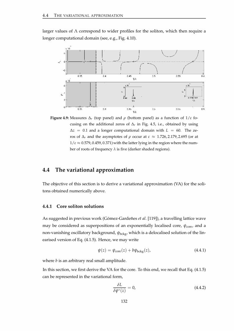
4.4 THE VARIATIONAL APPROXIMATION
larger values of Λ correspond to wider profiles for the soliton, which then require a
longer computational domain (see, e.g., Fig. 4.10).
Figure 4.9: Measures ∆r (top panel) and ρ (bottom panel) as a function of 1/ε fo-
cusing on the additional zeros of ∆r in Fig. 4.5, i.e., obtained by using
∆z = 0.1 and a longer computational domain with L = 60. The ze-
ros of ∆r and the asymptotes of ρ occur at ε ≈ 1.726, 2.179, 2.695 (or at
1/ε ≈ 0.579, 0.459, 0.371) with the latter lying in the region where the num-
ber of roots of frequency λ is five (darker shaded regions).
4.4 The variational approximation
The objective of this section is to derive a variational approximation (VA) for the soli-
tons obtained numerically above.
4.4.1 Core soliton solutions
As suggested in previous work (Gómez-Gardeñes et al. [119]), a travelling lattice wave
may be considered as superpositions of an exponentially localised core, ψcore, and a
non-vanishing oscillatory background, ψbckg, which is a delocalised solution of the lin-
earised version of Eq. (4.1.5). Hence, we may write
ψ(z) = ψcore(z) + bψbckg(z), (4.4.1)
where b is an arbitrary real small amplitude.
In this section, we first derive the VA for the core. To this end, we recall that Eq. (4.1.5)
can be represented in the variational form,
δL
δψ∗(z)= 0, (4.4.2)
132

4.4 THE VARIATIONAL APPROXIMATION
where δ/δψ∗ stands for the variational derivative of a functional and the Lagrangian is
L =∫ ∞
−∞
[
(2ε − Λ)|ψ|2 + ln(
1 + |ψ|2)
+ic
2
[
ψ∗ψ′ − ψ(ψ∗)′]
− ε
2ψ∗[ψ(z + 1) + ψ(z − 1)] + ψ[ψ∗(z + 1) + ψ∗(z − 1)]
]
dz. (4.4.3)
A suitable trial function, or ansatz, for the core may be chosen as
ψcore(z) = F(z) eipz, (4.4.4)
where
F(z) = A sech(az), (4.4.5)
with A, a and p non-zero real variational parameters. The ansatz is chosen because it
is an exact solution of the continuous nonlinear Schrödinger equation with cubic non-
linearity. While this ansatz postulates exponential tails of the soliton, the prediction
of solitons within the framework of the VA does not necessarily mean that the corre-
sponding solitons exist in a rigorous sense, as the actual tail may be non-vanishing at
|z| → ∞. In fact, the prediction of solitons by the VA may imply a situation in which
the amplitude of the nonvanishing tail is not zero, but attains its minimum (Kaup &
Malomed [128]).
The next step is to substitute ansatz (4.4.4) into Lagrangian (4.4.3), perform the integra-
tion, and derive the (stationary) Euler-Lagrange equations
∂L
∂A=
∂L
∂a=
∂L
∂p= 0. (4.4.6)
By substituting ansatz (4.4.4) into the Lagrangian and performing the integration, we
obtain the effective Lagrangian, as a function of parameters A, a and p,
Leff =2A2(2ε − Λ − cp) +A2
+ +A2−
a− 4A2ε cos(p)
sinh(a), (4.4.7)
where A± = ln(√
1 + A2 ± A)
.
Then, substituting Lagrangian (4.4.7) into Eqs. (4.4.6) yields
A(2ε − Λ − cp)
a+
A+
a√
1 + A2− 2Aε cos(p)
sinh(a)= 0, (4.4.8)
−2A2(2ε − Λ − cp) +A2+ +A2
−a2
+4A2ε cos(p) cosh(a)
sinh2(a)= 0, (4.4.9)
− c
a+
2ε sin(p)
sinh(a)= 0. (4.4.10)
This system of algebraic equations for A, a and p will be solved numerically.
133
4.4 THE VARIATIONAL APPROXIMATION
Before proceeding to the next section, it is noteworthy to mention that if one replaces
the term ln(
1 + |ψ|2)
in the Lagrangian (4.4.3) by its truncated expansions (up to some
order), then the new expression of the integral becomes a Lagrangian of a DNLS equa-
tion with polynomial nonlinearity. Therefore, using the ansatz (4.4.4), the effective
Lagrangian (4.4.7) can be used to determine an effective Lagrangian of a polynomial
DNLS equation whose the nonlinearity is a Taylor expansion of the transcendental
function. This is carried out by simply expanding the term (A2+ +A2
−)/a in Eq. (4.4.7),
which is the exact result of the integration of the transcendental function in Eq. (4.4.3),
with respect to A up to some order, depending on a polynomial DNLS system one
is interested in. For example, if one uses O(A4) and O(A6) expansions, the result-
ing effective Lagrangian corresponds to the cubic and cubic-quintic DNLS equations,
respectively.
Here, for the sake of comparison, we analyse the polynomial DNLS model
icψ′ + (2ε − Λ)ψ − ε [ψ(z + 1) + ψ (z − 1)] +(
1 − |ψ|2 + |ψ|4 − |ψ|6)
ψ = 0. (4.4.11)
The effective Lagrangian and the system of variational equations, by expanding (A2+ +
A2−)/a up to O(A8), are given, respectively, by
L′eff =
2A2(2ε − Λ + 1 − cp)
a− 2A4
3a+
16A6
45a− 8A8
35a− 4A2ε cos(p)
sinh(a), (4.4.12)
and
2ε − Λ + 1 − cp
a− 2A2
3a+
8A4
15a− 16A6
35a− 2ε cos(p)
sinh(a)= 0, (4.4.13)
−2ε − Λ + 1 − cp
a2+
A2
3a2− 8A4
45a2+
4A6
35a2+
2ε cos(p) cosh(a)
sinh2(a)= 0, (4.4.14)
− c
a+
2ε sin(p)
sinh(a)= 0. (4.4.15)
We also have computed the effective Lagrangian (4.4.12) directly by integrating a corre-
sponding Lagrangian of the polynomial DNLS equation and obtained the same result.
4.4.2 Prediction of the VA for embedded solitons
We now seek a condition for the possible existence of ESs. Following Kaup & Mal-
omed [128], we consider b in the general form of tailed solution (4.4.1) as an additional
variational parameter. Thus, a new variational equation,
∂L
∂b= 0, (4.4.16)
134

4.4 THE VARIATIONAL APPROXIMATION
must be added to the system of equations (4.4.10). By writing the integrand in the La-
grangian (4.4.3) as L(ψ, ψ∗, ψ′, (ψ∗)′), which is the Lagrangian density, differentiation
in Eq. (4.4.16) yields
∫ +∞
−∞
[
∂L∂ψ
ψbckg +∂L∂ψ∗ ψ∗
bckg +∂L∂ψ′ ψ
′bckg +
∂L∂(ψ∗)′
(ψ∗bckg)
′]
dz = 0. (4.4.17)
By integrating the third and the fourth terms by parts to obtain common factors ψbckg
and ψ∗bckg, respectively, and from the fact that
∂L∂(ψ∗)′
= − ic
2ψ, (4.4.18)
∂L∂ψ′ =
ic
2ψ∗, (4.4.19)
Eq. (4.4.17) becomes
∫ +∞
−∞
[(
∂L∂ψ∗ − d
dz
∂L∂(ψ∗)′
)
ψ∗bckg + c.c.
]
dz +
[
− ic
2ψψ∗
bckg + c.c.
]∞
−∞
= 0, (4.4.20)
where c.c. stands for the complex conjugate of the preceding expression.
As we are interested in solutions with the absence of nonzero backgrounds, one should
substitute ψ(z) in Eq. (4.4.20) with the solution form (4.4.1) by setting b = 0 (no tail).
This setting leads to the vanishing of the second term in the left-hand side of Eq. (4.4.20).
Therefore, the condition for the possible existence of ESs is given by a natural orthogo-
nality relation,
∫ +∞
−∞
δL/δψ∗|ψ(z)=ψcore(z)ψ∗
bckg(z) + c.c.
dz = 0, (4.4.21)
where the variational derivative δL/δψ∗|ψ(z)=ψcore(z)is the left-hand side of Eq. (4.1.5)
with ψ(z) replaced by ψcore(z).
In the context of the VA, ψcore(z) in Eq. (4.4.21) should be substituted by the (approxi-
mate) form (4.4.4) corresponding to the soliton. Here, the background function is taken
as
ψbckg(z) = eiλz, (4.4.22)
which is nothing other than the linear solution (4.2.1). Note that this background func-
tion is a crude approximation because to the leading order ψbckg should satisfy the
linearised equation of (4.1.5) about ψcore with the limiting properties ψbckg → eiλz as
z → ±∞.
The substitution of Eqs. (4.4.4) and (4.4.22) into Eq. (4.4.21) yields
∫ ∞
−∞M(z)dz = 0, (4.4.23)
135
4.4 THE VARIATIONAL APPROXIMATION
where
M(z) = −ε [F(z + 1) cos((λ − p)z − p) + F(z − 1) cos((λ − p)z + p)]
+
(2ε − cλ − Λ) F(z) +F(z)
1 + F(z)2
cos((λ − p)z). (4.4.24)
It is readily checked that M(z) is an even function. Therefore, after some manipula-
tions, integral relation (4.4.23) may be cast into the form
∫ ∞
0
[
(2ε − cλ − Λ) cos((λ − p)z)
cosh(az)− 2 cosh(az) cos((λ − p)z)
cosh(2az) + 1 + 2A2
−Bε cos((λ − p)z) cosh(az)
cosh(2az) + cosh(2a)+
Cε sin((λ − p)z) sinh(az)
cosh(2az) + cosh(2a)
]
dz = 0,(4.4.25)
where B = 4 cos(p) cosh(a) and C = 4 sin(p) sinh(a). The integrals in each term can be
evaluated using the formulas (Gradshteyn & Ryzhik [129])
(i)∫ ∞
0
cos(ax)
cosh(
b
2 x)dx =
π
b cosh(
aπb
) , (4.4.26)
provided Re(b) > 0 and a ∈ R;
(ii)∫ ∞
0
cos(ax) cosh(
b
2 x)
cosh(bx) + cosh(c)dx =
π cos(
ac
b
)
2b cosh(
c
2
)
cosh(
aπb
) , (4.4.27)
provided πRe(b) > |Im(b∗c)|;
(iii)∫ ∞
0
cos(ax) cosh(
b
2 x)
cosh(bx) + ddx =
π cos(
a
bcosh−1(d)
)
2b cosh(
12 cosh−1(d)
)
cosh(
aπb
)
, (4.4.28)
provided πRe(b) > |Im(b∗ cosh−1(d))|;
(iv)∫ ∞
0
sin(ax) sinh(
b
2 x)
cosh(bx) + cos(e)dx =
π [χ+ − χ−]
b sin(e)[
cosh(
2aπb
)
− cos (π)] , (4.4.29)
where χ± = sin(
12(π ∓ e)
)
sinh(
a
b(π ± e)
)
, provided πRe(b) > |Re(b∗e)|,Re(b) > 0 and a > 0.
Substituting a = λ − p, b = c = 2a, d = 1 + 2A2 and e = 2ai into Eqs. (4.4.26)–(4.4.29),
the calculation for the integration (4.4.25) yields
E ≡ (2ε − cλ − Λ)− 2ε cos(λ) +
cos
(
1
2a
[
(λ − p) cosh−1(1 + 2A2)]
)
cosh
(
1
2
[
cosh−1(1 + 2A2)]
) = 0, (4.4.30)
provided a > 0 and λ > p. Thus, in the framework of the VA, along with the results
of the VA for the soliton’s core given by Eqs. (4.4.8)–(4.4.10) and with the root(s) λ of
Eq. (4.2.3), we may predict a curve E as a function of (ε, c, Λ) along which the existence
of the ESs may be expected, i.e., when E = 0.
136

4.4 THE VARIATIONAL APPROXIMATION
If we expand E with respect to A up to O(A8), we arrive at the following form:
E′ ≡ (2ε− cλ−Λ+ 1)− 2ε cos(λ)+3
∑k=1
[
(−1)k
(2k)!
(
A
a
)2k k
∏j=1
(
(λ − p)2 + (a(2j − 1))2)
]
= 0,
(4.4.31)
which is the corresponding result of the integral relation (4.4.21) for the polynomial
DNLS (4.4.11). The same result for E′ is also obtained through the integration of poly-
nomial terms which confirms the validity of the result in Eq. (4.4.30). As we discuss
later in Section 4.5.2, Eq. (4.4.31) is useful to support our conjecture regarding the use
of VA in searching for ESs in the saturable DNLS model.
4.4.3 The VA-based stability analysis
Here, we propose to use the VA to study the stability of the core of the travelling lat-
tice solitary wave by calculating eigenvalues for modes of small perturbations in the
moving coordinate frame, following Flytzanis et al. [130]. The stability of the back-
ground, i.e., the modulational (in)stability of the plane lattice waves, was studied by
Gómez-Gardeñes et al. [119].
The Lagrangian of the time-dependent equation (4.1.4) is
L =∫ ∞
−∞
[
(2ε − Λ)|ψ|2 + ln(
1 + |ψ|2)
+ic
2[ψ∗ψz − ψψ∗
z ]
− ε
2ψ∗[ψ(z + 1, τ) + ψ(z − 1, τ)] + ψ[ψ∗(z + 1, τ) + ψ∗(z − 1, τ)]
− i
2(ψ∗ψτ − ψψ∗
τ)
]
dz. (4.4.32)
Note that Eq. (4.1.4) is produced by the variation with respect to ψ∗ from the action
functional S =∫
Ldτ, not from the Lagrangian (4.4.32). However, for practical pur-
poses (the derivation of VA equations), it is enough to calculate Lagrangian (4.4.32) (it
is not necessary to calculate the action functional explicitly).
A time-dependent ansatz, generalising the static one (4.4.4), is
ψcore(z, τ) = A(τ)sech [a(τ)(z − ξ(τ))] e(iφ(τ)+ip(τ)z+ i2 C(τ)[z−ξ(τ)]2), (4.4.33)
where all parameters are real functions of time. Additional variational parameters
which appear here are the coordinate of soliton’s centre, ξ(τ), the overall phase, φ(τ),
and the intrinsic chirp, C(τ). In particular, the inclusion of the chirp in the above ansatz
was due to Anderson [131]. Substituting ansatz (4.4.33) into Lagrangian (4.4.32) and
137

4.5 COMPARISONS: NUMERICS VS ANALYTICS
performing the integration yields the corresponding effective Lagrangian,
Leff = A(τ)2
−2Λ + εQ(τ) + 2 [ξ(τ)p′(τ) + φ′(τ)− cp(τ)]
a(τ)+
π2C′(τ)12a(τ)3
+ln2(
√
1 + A(τ)2 + A(τ))
+ ln2(
√
1 + A(τ)2 − A(τ))
a(τ), (4.4.34)
with primes standing for the derivatives, and
Q(τ) = 4 −4π sin
(
C(τ)2
)
cos (p(τ))
sinh (a(τ)) sinh(
C(τ)π2a(τ)
)
= 4 − 4a(τ) cos(p(τ))
sinh(a(τ))+
(a(τ)2 + π) cos(p(τ))C(τ)2
6a(τ) sinh(a(τ))+O(C4).(4.4.35)
The (dynamical) Euler–Lagrange equations for the variational parameters take the form
of a nonlinear ODE system, which can be symbolically written in the vectorial form,
x = g(x), (4.4.36)
where x = [A(τ), a(τ), p(τ), C(τ), φ(τ), ξ(τ)]T . The VA-predicted linear stability anal-
ysis is based on the linearisation ansatz,
x = x0 + δyeΩτ, δ ≪ 1; Ω ∈ C, (4.4.37)
where x0 = [A0, a0, p0, 0, 0, 0]T represents the steady state solution of the core soliton
with (A0, a0, p0) satisfying the system of variational equations (4.4.8)–(4.4.10). The sub-
stitution of Eq. (4.4.37) into Eq. (4.4.36) and the linearisation in δ lead to the eigenvalue
problem,
Hy = Ωy, (4.4.38)
with the corresponding stability matrix H. The stability of the stationary solution x0 is
then determined by the eigenvalues Ω, which must be found in a numerical form; the
solution x0 is stable if Re(Ω) ≤ 0 for all eigenvalues.
4.5 Comparisons: numerics vs analytics
4.5.1 The soliton’s core
For given parameters ε, c and Λ, we solved the variational equations (4.4.8)–(4.4.10)
to produce suitable real solutions A, a and p, which then give a quasi-analytical ap-
proximation for the soliton’s core described by function ψcore(z) (see Eq. (4.4.4)). As
generic examples, in Fig. 4.10 we present, at ε = 1 and c = 0.7, the comparison of two
138

4.5 COMPARISONS: NUMERICS VS ANALYTICS
soliton profiles obtained from the numerical results and VA for two different values of
Λ. We have found A ≈ 1.228, a ≈ 0.554, p ≈ 0.377 for Λ = 0.5 (Fig. 4.10(a)), and
A ≈ 0.685, a ≈ 0.414, p ≈ 0.368 for Λ = 0.7 (Fig. 4.10(b)). Particularly good agreement
is observed in both cases.
−10 −5 0 5 10−0.6
−0.4
−0.2
0
0.2
0.4
0.6
0.8
1
1.2
1.4
z
Re(
ψ),
Im(ψ
)
(a) ε = 1, c = 0.7, and Λ = 0.5
−10 −5 0 5 10−0.4
−0.2
0
0.2
0.4
0.6
0.8
z
Re(
ψ),
Im(ψ
)
(b) ε = 1, c = 0.7, and Λ = 0.7
Figure 4.10: The comparison of two soliton profiles for two different values of Λ, as
indicated in the caption to each panel. The solid lines correspond to nu-
merical results, i.e., solutions of Eq. (4.3.4) imposed by constraints (4.3.8),
with ∆z = 0.2 and L = 50 (the z-axis is truncated to focus the picture
on the soliton’s core), both the real and imaginary parts being shown.
The dotted lines are predictions of the variational approximation through
solving system of Eqs. (4.4.8)–(4.4.10).
As we have considered the polynomial DNLS (4.4.11) in our VA calculations, here we
also present the comparison of two profiles of the soliton’s core, which are calculated
from numerics and VA formulations for two different sets of parameter values; this is
shown in Fig. 4.11. The obtained variational parameters in Figs. 4.11(a) and 4.11(b) are
(A, a, p) ≈ (1.034, 0.338, 0.071) and (A, a, p) ≈ (0.668, 0.426, 0.369), respectively. As in
the case of the saturable DNLS system, we observe from the figures that the VA-based
analytical calculations for the polynomial DNLS equation are also in a good agreement
with the corresponding numerical results.
To further confirm the agreement for different values of Λ, ε and c, in the following we
compare parameters A, a and p produced by the VA with their numerical counterparts
(we only do this for the saturable case). To calculate the latter, we make use of the
following relations, which are generated by ansatz (4.4.4) at z = 0:
ψ(0) = A, ψ′(0) = ipA, ψ′′(0) = −A(a2 + p2). (4.5.1)
Thus, using the central finite differences, we obtain the numerical counterparts of A, p
139

4.5 COMPARISONS: NUMERICS VS ANALYTICS
−20 −15 −10 −5 0 5 10 15 20−0.2
0
0.2
0.4
0.6
0.8
1
1.2
z
Re(
ψ),
Im(ψ
)
(a) ε = 5, c = 0.7, and Λ = 0.5
−10 −5 0 5 10−0.4
−0.2
0
0.2
0.4
0.6
0.8
z
Re(
ψ),
Im(ψ
)
(b) ε = 1, c = 0.7, and Λ = 0.7
Figure 4.11: As Fig. 4.10 but for the polynomial DNLS equation (4.4.11) where the VA
solutions for the soliton’s core are obtained through solving Eqs. (4.4.13)–
(4.4.15).
and a as
Anum = ψ N+12
, (4.5.2)
pnum =Im(
ψ N+12 +1
)
− Im(
ψ N+12 −1
)
2Anum∆z, (4.5.3)
anum = ±
√
√
√
√−Re(
ψ N+12 −1
)
− 2Re(
ψ N+12
)
+ Re(
ψ N+12 +1
)
Anum(∆z)2− p2
num. (4.5.4)
The comparison of parameters (A, a, p) obtained numerically (solid lines) and from the
VA (dashed lines) is shown in Fig. 4.12(a) for varying 1/ε and fixed (c, Λ) = (0.7, 0.5).
In that figure we only take the positive value of a in Eq. (4.5.4) to make it in accor-
dance with the VA. We observe that the solid and dashed lines are generally close for
all the three parameters. Nevertheless, we also obtain isolated values of 1/ε, which
behave as singular points. Near the singularities the numerical results deviate very
rapidly from the predictions of the VA. In fact, at these singular points the numerically
obtained solutions are strongly delocalised due to the resonance of the oscillating tails
with the finite size of the computational domains (compare these points with those in
Fig. 4.14(a)). Hence, the positions of such singularities depend on L and they may be
considered as artifacts of approximating the infinite region by the finite domain.
Next, as in Fig. 4.10, where a better approximation is obtained for larger Λ, we also
observe in Fig. 4.12(b) that the variational and numerical curves for A, a, p are closer
for Λ = 0.7 than those in 4.12(a). In the latter case, the singularities are present too,
even though they are less pronounced here.
To obtain a full description of the effect of Λ on the validity of the VA, let us now
140

4.5 COMPARISONS: NUMERICS VS ANALYTICS
0.7 0.8 0.9 1 1.1 1.2 1.3 1.4 1.50.2
0.4
0.6
0.8
1
1.2
1.4
1/ε
A, a
, p
A
a
p
(a) (c, Λ) = (0.7, 0.5)
0.7 0.8 0.9 1 1.1 1.2 1.30.2
0.3
0.4
0.5
0.6
0.7
0.8
1/ε
A, a
, p
A
a
p
(b) (c, Λ) = (0.7, 0.7)
Figure 4.12: The comparison of parameters (A, a, p) calculated from the numerical
data (solid lines) through Eqs. (4.5.2)–(4.5.4), and from the VA (dashed
lines) through Eqs. (4.5.1), for varying 1/ε and fixed (c, Λ), as shown in
the caption of each panel.
0.3 0.4 0.5 0.6 0.7 0.80
0.2
0.4
0.6
0.8
1
1.2
1.4
1.6
1.8
2
Λ
A, a
, p
Ap
a
Figure 4.13: As Fig. 4.12 but for varying Λ and fixed (ε, c) = (1, 0.7).
141

4.5 COMPARISONS: NUMERICS VS ANALYTICS
examine (A, a, p) as functions of Λ for fixed (ε, c) = (1, 0.7), which is presented in
Fig. 4.13. From the figure, we can confirm that the VA is more accurate for larger Λ.
This agreement still holds even when the solutions become wide and vanish indicated
by a → 0 and A → 0, respectively.
From the comparisons presented in Figs. 4.12 and 4.13 above, we can conclude that
the VA provides a reliable approximation for the soliton’s core. Nevertheless, the
VA as well as our numerics are not capable of exploring the regime close to the anti-
continuum limit. We observed that the amplitude of the oscillating tails of the numeri-
cal solutions increases as ε decreases, which creates a problem in the convergence of our
numerical continuation. We also noted that the amplitude A in the ansatz (4.4.4) de-
creases as ε decreases and vanishes at a threshold point of ε. It is not yet clear whether
or not there is embedded soliton close to the anti-continuum limit.
4.5.2 Embedded solitons
For the sake of comparisons, let us first plot the measure ∆r as a function of 1/ε for
the parameter values (Λ, c, ∆z, L) used in Figs. 4.10(a) and 4.10(b), which are shown,
respectively, in Figs. 4.14(a) and 4.15(a). One should notice that the former figure is
basically similar to Fig. 4.5(a) but with a longer computational domain and a shorter
interval of 1/ε, whereas the latter is replotted from the top panel of Fig. 4.6(b) by cutting
the domain of 1/ε.
Next, to predict the location of ESs in the framework of the VA, as explained in the
previous section, we substitute the solution of Eqs. (4.4.8)–(4.4.10) and the root(s) λ
of Eq. (4.2.3) into Eqs. (4.4.30) to find E as a function of ε, c and Λ. Therefore, the
existence of ESs can be predicted by seeking for the values of parameters at which
E = 0. For the parameter values used in Figs. 4.14(a) and 4.15(a), curves for E are
displayed, respectively, in Figs. 4.14(b) and 4.15(b). It is seen that E 6= 0 in both figures,
i.e., genuinely localised solitons cannot be directly predicted by the VA.
However, we can propose a conjecture, based on a “phenomenological” consideration
of the figures, that there are two zeros of ∆r on the left and right of a maximum of
E. For example, in Fig. 4.14 we have the maximum of E at ε ≈ 0.853 (i.e., at 1/ε ≈1.172), which is located between two adjacent numerically found zeros of ∆r. The same
phenomenon also takes place in Fig. 4.15, where two zero-crossing points lie between a
maximum of E, i.e., at ε ≈ 1.020 (i.e., at 1/ε ≈ 0.980). We have also computed the signed
measure ∆r and E for other combinations of parameter values, where we observed
the same pattern (see, e.g., Fig. 4.16). Thus, we conclude that, with the addition of a
142

4.5 COMPARISONS: NUMERICS VS ANALYTICS
0.7 0.8 0.9 1 1.1 1.2 1.3 1.4 1.5
−3
−2
−1
0
1
2
3
x 10−3
1/ε
∆ r
(a)
0.7 0.8 0.9 1 1.1 1.2 1.3 1.4 1.5−2
−1.8
−1.6
−1.4
−1.2
−1
−0.8
−0.6
−0.4
−0.2
0
1/ε
E
(b)
Figure 4.14: (a) The signed measure ∆r (cf. Eq. (4.3.10)) as a function of 1/ε for c = 0.7,
Λ = 0.5, ∆z = 0.2 and L = 50, where ∆r is zero at ε ≈ 0.737, 0.988, 1.306
(or at 1/ε ≈ 1.357, 1.012, 0.766), as shown by empty circles. (b) E ver-
sus 1/ε (cf. Eq. (4.4.30)), for the same parameter values (Λ, c) as in
panel (a) and for the corresponding (A, a, p) and root(s) λ obtained from
Eqs. (4.4.8)-(4.4.10) and Eq. (4.2.3), respectively. It is clearly seen that
E 6= 0 in the observed domain of 1/ε. However, we can conjecture
that ESs are located near the maximum of E, i.e., at ε ≈ 0.853 (or at
1/ε ≈ 1.172), as indicated by the star.
143

4.5 COMPARISONS: NUMERICS VS ANALYTICS
0.7 0.8 0.9 1 1.1 1.2 1.3
−1.5
−1
−0.5
0
0.5
1
1.5
x 10−5
1/ε
∆ r
(a)
0.7 0.8 0.9 1 1.1 1.2 1.3−2
−1.8
−1.6
−1.4
−1.2
−1
−0.8
−0.6
−0.4
−0.2
0
1/ε
E
(b)
Figure 4.15: The same as Fig. 4.14, but for Λ = 0.7. Zeros of ∆r are found at
ε ≈ 0.828, 1.158 (or at 1/ε ≈ 1.208, 0.864), which are the same as those in
Fig. 4.6(b), and the maximum of E occurs at ε ≈ 1.020 (or at 1/ε ≈ 0.980).
144

4.5 COMPARISONS: NUMERICS VS ANALYTICS
constant, function E may be able to predict the location of ESs. We suspect that the
missing constant, which amounts to the shift of the plot for E vertically, is related to
the choice of the ansatz (see, e.g., Boyd [132] for different ansatz accounting for the
oscillating tails).
0.3 0.4 0.5 0.6 0.7 0.8−5
−4
−3
−2
−1
0
1
2
3
4
5x 10
−3
Λ
∆ r
(a)
0.3 0.4 0.5 0.6 0.7 0.8−1.5
−1
−0.5
0
Λ
E
(b)
Figure 4.16: As Fig. 4.14, but with the signed measure ∆r being a function of Λ (for
fixed c = 0.7, ε = 1, ∆z = 0.2 and L = 50). Zeros of ∆r are found at
Λ ≈ 0.515, 0.772 and curve E is maximum at Λ ≈ 0.714.
To support further our conjecture, we also plot the same quantities as those presented
in the previous figures, but now for the polynomial DNLS (4.4.11). These plots are
shown in Fig. 4.17 by using parameter values as in Fig. 4.11(b). From the top panel of
the figure, we can see clearly that ∆r 6= 0 along the observed domain of 1/ε, which
indicates that the polynomial DNLS (4.4.11) does not support the travelling lattice soli-
tons with vanishing tails. Most interestingly, as shown in the bottom panel, the curve
E′ does not have any local maximum, which is in accordance with the contraposition
statement of our conjecture for the saturable DNLS.
4.5.3 Stability
To determine the stability of the soliton based on the VA, we have solved the eigenvalue
problem (4.4.38). For the soliton shown in Fig. 4.10(a), i.e., with x0 ≈ [1.228, 0.554, 0.377,
145

4.5 COMPARISONS: NUMERICS VS ANALYTICS
(a)
(b)
Figure 4.17: As Fig. 4.14 but for the polynomial DNLS (4.4.11) where ln (|E′|) (see ex-
pression (4.4.31)) is plotted. The parameter values used are the same as in
Fig. 4.11(b). The number of roots λ, which is indicated by the white (one
root), light shaded (three roots) and dark shaded (five roots) regions (see
cf. Fig. 4.2(b)), are the same as the number of curves E′ in the correspond-
ing regions.
146

4.6 A FAILURE OF THE FINITE-DIFFERENCE METHOD: NUMERICAL STABILITY
0, 0, 0]T , we obtain the corresponding eigenvalues Ω ≈ 0, 0, 0, 0, 0.436i,−0.436i. For the
soliton in Fig. 4.10(b), i.e., x0 ≈ [0.685, 0.414, 0.368, 0, 0, 0]T, the corresponding eigenval-
ues are Ω ≈ 0, 0, 0, 0, 0.225i,−0.225i. As the real part of all the eigenvalues is zero, we
conclude that both solitons are stable. These results are in agreement with the numerical
findings of Melvin et al. [66].
4.6 A failure of the finite-difference method: numerical stabil-
ity
To examine the stability of the numerically obtained solutions to Eq. (4.1.1), recall the
time-dependent model (4.1.4). Introducing the linearisation ansatz ψ(z, τ) = ψ(z) +
δ(r(z)eiµτ + s∗(z)e−iµ∗τ), with |δ| ≪ 1 being a small perturbation amplitude and with
the asterisk indicating complex conjugation, into Eq. (4.1.4), we thereby obtain the lin-
ear eigenvalue problem (EVP) for the stability of ψ(z), given by
− µ
(
r
s
)
=
L+ − ψ2
(1 + |ψ|2)2
ψ∗2
(1 + |ψ|2)2L−
(
r
s
)
= H(
r
s
)
, (4.6.1)
where we have introduced the operators
L± ≡ icd
dz±[
(2ε − Λ)− ε∆1 +1
(1 + |ψ|2)2
]
, (4.6.2)
with ∆1x(z) = x(z+ 1) + x(z− 1). The stability of the solution ψ(z) is then determined
by the eigenvalues of Eq. (4.6.1). It is clear that the solution is unstable if and only
if there is at least one eigenvalue µ with a negative imaginary part. Here, we then
solve Eq. (4.6.1) numerically by means of the finite-difference method, as previously
discussed in Section 4.3.
For a soliton that corresponds to one of the zero crossings in Fig. 4.15(a), i.e., ε = 1.158,
we present in Fig. 4.18(a) the EVP spectra in the complex plane. As there are eigen-
values with negative imaginary parts, the soliton is unstable. We show in Fig. 4.18(b)
combination of the eigenfunction (r + s∗) corresponding to the most unstable eigen-
value, which demonstrate that the eigenfunction is indeed localised. These results are
in contrast to our VA stability and the numerical results of Melvin et al. [66] obtained
by calculating the corresponding Floquet multipliers, where the solitons were shown
to be linearly stable.
To understand the discrepancy, we investigate the effect of the grid spacing ∆z on the
EVP (4.6.1). By using the same parameter values, we show in Fig. 4.18(a) the distribu-
147
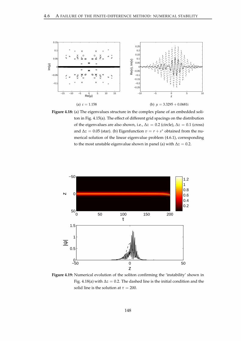
4.6 A FAILURE OF THE FINITE-DIFFERENCE METHOD: NUMERICAL STABILITY
−15 −10 −5 0 5 10 15
−0.1
−0.05
0
0.05
0.1
0.15
Re(µ)
Im(µ
)
(a) ε = 1.158
−10 −5 0 5 10
−0.25
−0.2
−0.15
−0.1
−0.05
0
0.05
0.1
0.15
0.2
0.25
z
Re(
v), I
m(v
)
(b) µ = 3.3295 + 0.0681i
Figure 4.18: (a) The eigenvalues structure in the complex plane of an embedded soli-
ton in Fig. 4.15(a). The effect of different grid spacings on the distribution
of the eigenvalues are also shown, i.e., ∆z = 0.2 (circle), ∆z = 0.1 (cross)
and ∆z = 0.05 (star). (b) Eigenfunction v = r + s∗ obtained from the nu-
merical solution of the linear eigenvalue problem (4.6.1), corresponding
to the most unstable eigenvalue shown in panel (a) with ∆z = 0.2.
τ
z
0 50 100 150 200
−50
0
50
−50 0 500
0.5
1
1.5
z
|ψ|
0.20.40.60.811.2
Figure 4.19: Numerical evolution of the soliton confirming the ‘instability’ shown in
Fig. 4.18(a) with ∆z = 0.2. The dashed line is the initial condition and the
solid line is the solution at τ = 200.
148

4.7 CONCLUSION
tion of the eigenstructures for ∆z = 0.2, ∆z = 0.1 and ∆z = 0.05, where we obtain that
the smaller the ∆z, the more unstable eigenvalues one will gain. This contradicts the
common intuition that a discrete approximation will converge to the continuous limit
for a small enough ∆z. We believe that the spurious instability is caused by the numer-
ical approximation of the advance–delay terms. The instability can indeed be observed
in the time-dynamics of the advance–delay-differential equation (4.1.4) as shown in Fig.
4.19, where we have used the same spatial discretization and a Runge-Kutta method for
the time integration. One can see that the soliton suffers from high-frequency unstable
modes, as predicted by the unstable eigenfunctions in Fig. 4.18(b).
One possible solution to resolve the discrepancy is to use the pseudo-spectral method
as suggested and successfully applied in a Fermi-Pasta-Ulam equation by Flytzanis et
al. [130]. This issue will be studied further.
4.7 Conclusion
The aim of this work was to revisit the general problem of the existence and stability
of travelling localised pulses in discrete models based on the one-dimensional discrete
nonlinear Schrödinger (DNLS) equation with saturable nonlinearity. After analysing
the linear spectrum of the model, carried out through numerical calculations and per-
turbation analyses, we obtained the bifurcation diagram of the spectral bands. Ac-
cording to Melvin et al. [66, 67], finding genuinely localised solutions by varying one
parameter only becomes possible within parameter regions of the spectral bands in
which there is a single resonance with linear waves.
In the aforementioned references, it was demonstrated that the DNLS equation with
saturable onsite nonlinearity admits isolated genuine travelling-soliton states. In this
work, we have used a numerical scheme to solve the saturable DNLS equation in a
moving coordinate frame, which is an advance–delay-differential equation. By us-
ing a Newton–Raphson method, together with a measure for the tails (either the one
modified from that proposed by Melvin et al. [66, 67] or our alternative measure), we
confirmed the existence of genuinely travelling discrete solitons, which are embedded
solitons (ESs). We showed that the outputs from our numerical scheme, for a grid spac-
ing small enough and a computational domain large enough, are identical with those
reported in [66].
In addition to the numerical work, we have developed a semi-analytical approach for
seeking travelling solitons, based on the application of the variational approximation
(VA) to the advance–delay-differential form of the saturable DNLS equation in the
149

4.7 CONCLUSION
moving coordinate frame. The approximated (core) solitons are in good agreement
with the corresponding numerical findings. The VA was also derived to examine the
stability of the travelling solitons which shows that they are stable, i.e., in agreement
with [66]. Moreover, the VA was also developed to predict the locations of travelling
lattice solitons with strictly vanishing tails and the relevance of the results was dis-
cussed.
Although we obtained the solutions reported in [66] through our numerical scheme, we
showed that the corresponding scheme for the eigenvalue problem did not produce the
correct results. This discrepancy is left for future investigation.
150

CHAPTER 5
Conclusion
In this thesis, we have examined the existence and stability of discrete solitons in two
main lattice models, i.e., cubic and saturable discrete nonlinear Schrödinger (DNLS)
equations. In the cubic-type model, we considered stationary discrete solitons under
the effect of parametric driving and/or damping. In the saturable-type model, we
studied travelling lattice solitons. Let us now summarise the work and the main results
obtained in the abovementioned studies as well as point out several problems that
would be interesting to consider in the future.
5.1 Summary
We began our discussion in Chapter 1 by providing background information about
solitons and the considered lattice equations. These include a definition and historical
development of (discrete) solitons, and a general review of the DNLS equations. In par-
ticular, we outlined the development of theoretical and experimental studies of discrete
solitons in the context of two applications, i.e., optical waveguide arrays and systems
of micro- and nanoelectromechanical (MEMS and NEMS) resonators. Moreover, in
the same chapter, we presented preliminary analyses of stationary and travelling dis-
crete solitons in the cubic and saturable DNLS models. Some analytical methods used
throughout this thesis were also reviewed briefly in this chapter.
In Chapter 2 we investigated a parametrically driven discrete nonlinear Schrödinger
(PDNLS) equation, i.e., a cubic DNLS model with the inclusion of parametric driving
with strength γ. The existence and stability of fundamental (onsite and intersite) bright
and dark discrete solitons were discussed both analytically and numerically. Our anal-
yses relied on the anticontinuum (AC) limit approach from which we can employ a
perturbation expansion to approximate the fundamental soliton solutions for the case
151

5.1 SUMMARY
of small coupling constant ε. In carrying out the examination of the stability of soli-
tons, we solved numerically a corresponding eigenvalue problem (EVP) from which
we obtained the stability region in the (ε, γ)-plane. Analytical calculations of the EVP
based on a perturbation method were also derived to predict the onset of instability
for each soliton. Moreover, to confirm the typical dynamics of solitons in the stable
and unstable parameter regions, we performed numerical integrations of the PDNLS
equation. All of the aforementioned analyses were presented in Sections 2.2 and 2.3 for,
respectively, bright and dark solitons.
From our studies above, we obtained that our analytical calculations, for small ε, are
generally consistent with the numerics. Regarding the effect of parametric driving on
the stability results, we found that undriven onsite bright solitons, which are stable for
any coupling constant, and onsite dark solitons, which are stable for small coupling
constant, can be destabilised by a parametric driving; for the onsite bright soliton, this
result has been reported earlier by Susanto et al. [91]. By contrast, intersite bright and
dark solitons, which were shown to be always unstable in the undriven case, can be
stabilised by the driving. Interestingly, we also found a range of values of γ in which a
discrete dark soliton is stable for all ε.
Additional work in Chapter 2, discussed in Section 2.4, was on the application of a
PDNLS model in arrays of parametrically-driven MEMS and NEMS resonators. By
using a multiscale expansion method, we showed that our DNLS equation can be de-
rived from a governing equation of MEMS and NEMS resonators, i.e., a particular type
of parametrically driven discrete Klein–Gordon equation. The numerical integrations
of the Klein–Gordon system were then demonstrated to confirm the relevance of our
stability findings in the PDNLS model. From the results of the latter work, we con-
cluded that the parametrically driven DNLS equation can be used to describe, under
certain conditions, the behaviour of MEMS and NEMS resonators.
Next, in Chapter 3, we extended the ideas of Chapter 2 by introducing a damping term
with strength α in the PDNLS system. A study for such a model, called a paramet-
rically driven damped discrete nonlinear Schrödinger (PDDNLS) equation, was per-
formed for onsite and intersite bright solitons (in focusing PDDNLS). We identified
that there exist two and four types of onsite and intersite discrete solitons, respectively.
We called those solutions onsite type I and II, and intersite type I, II, III and IV, where
the last two types are essentially the same, due to symmetry. We observed that the
type I solution for onsite and intersite solitons, which can be unstable in the case of no
dissipation, can be stabilised by the damping, whereas the other types of solution are
always unstable. We also found an interval of values of α in which the onsite type I is
152

5.1 SUMMARY
stable for all ε. Our further analysis demonstrated that the onsite type I and II expe-
rience a saddle-node bifurcation where the limit point is achieved when the damping
and driving strengths are equal (for any coupling constant). The same bifurcation was
also shown to be undergone by the intersite type I and II. Furthermore, we observed a
pitchfork bifurcation occurring in intersite type I, III and IV. The corresponding branch
points for such a bifurcation in the (ε, α)-plane have been calculated analytically, for
small ε, and numerically.
The most interesting result in the study of PDDNLS equation is the existence of peri-
odic solitons (limit cycles) which emerge from Hopf bifurcations experienced by onsite
type I, intersite type I and intersite type III-IV. By using the numerical continuation soft-
ware Matcont, we performed continuations of the corresponding limit cycles as well as
the stability of the periodic solitons; this was discussed in Section 3.5. We found subcrit-
ical Hopf bifurcations along the existence curve of the onsite type I and intersite type
III-IV. In addition, we observed three Hopf bifurcations for intersite type I, of which
two were shown to be supercritical.
Next, in Chapter 4 we discussed the existence and stability of travelling solitary waves
in the DNLS model with saturable nonlinearity. This study basically followed the idea
of Melvin et al. [66, 67] who initially investigated the problem using a pseudo-spectral
numerical scheme.
As noted in the abovementioned references, a travelling solitary wave of the saturable
DNLS equation would be easy to seek by varying one parameter only. This becomes
possible if one can identify the parameter regions of the spectral bands where a single
resonance of the travelling solitons with plane waves occurs. To do this, we examined
the linear spectrum of the model in the travelling wave frame, i.e., an advance–delay-
differential equation, carried out numerically, as done by Melvin et al. [66, 67], and
analytically through a perturbation expansion. This analysis was presented in Section
4.2.
To solve numerically the travelling solutions in the saturable model, i.e., via the advance-
delay-differential equation, we applied a finite difference discretization. From this
scheme, we had a system of difference equations which was then solved using a Newton-
Raphson method. Since the obtained solutions were generally accompanied by nonzero
oscillatory tails, as suggested in the latter references, we need to add an extra tail con-
dition to find solutions with vanishing tails, i.e., embedded solitons (ESs). For this
condition, we used the measure which was modified from that proposed by Melvin et
al. [66, 67], corroborated by our alternative measure. For a grid spacing small enough
and a computational domain large enough, we showed that the results produced from
153

5.2 FUTURE WORK
our numerical scheme are consistent with those in [66, 67]. The numerical works above
were given in Section 4.3.
For the analytical part of our study in Chapter 4, presented in Section 4.4, we employed
a variational approximation (VA). We observed that the approximated (core) solitons
are in good agreement with the corresponding numerical results. The VA-based sta-
bility analysis was also performed, showing that the solutions are stable, i.e., in accor-
dance with that reported by Melvin et al. [66]. In addition, we also derived the VA to
predict the locations of the ESs. In the latter work, our analytical prediction could not
be verified numerically and we argued that this is related to the choice of the ansatz
for the tails as discussed in the chapter. The condition when there are two waves in
the linear spectrum is indeed another case that our tail will fail, even though it is still a
big question whether embedded solitons exist at all in such a case, as explained in the
chapter.
5.2 Future work
In this section, we note several problems that could be interestingly proposed as future
work. Some of them arise from the extension of the ideas in the present work, while the
others emerge from the questions raised in the course of our study which need further
investigations.
One possible problem is to expand the work of Chapter 2 to, e.g., a twisted localised
mode. In the absence of parametric driving, such a solution has been considered, e.g.,
by Kevrekidis et al. [114] where it was shown that it is stable for small coupling con-
stant. Unlike the case of an undriven intersite soliton with in-phase oscillation where
the bifurcating unstable eigenvalues lie along the imaginary axis of the spectral plane,
the instability of the out-of-phase intersite mode occurs because of the presence of a
quartet of complex eigenvalues. Thus, its typical dynamics is in the form of an unsta-
ble breather. Moreover, it was also shown that an undriven twisted soliton experiences
a saddle-node bifurcation, and this must be also the case in the driven mode.
Another interesting problem that could be pursued in the future is the study of dark
solitons in the defocusing PDDNLS equation. For the case of bright solitons in the
focusing PDDNLS model, it was already shown in this thesis that these solutions have
rich dynamical localisation effects, including the existence of periodic solitons. Thus,
one could immediately predict that dark solitons in the driven and damped DNLS
equation will also permit such interesting properties. In addition, the existence and
stability of a twisted discrete soliton in the PDDNLS system would be also interesting
154

5.2 FUTURE WORK
to investigate.
The interaction of stable standing waves and perturbations in the PDDNLS system is
also interesting. From equation (3.1.1), we note the balance equation
id
dt|φn|2 = ε(Jn − Jn−1)− 2iα|φn|2 + γ(φ
2n − φ2
n), (5.2.1)
where Jn = φn+1φn − φn+1φn. For simplicity, consider the case ε = 0. Perturbing the
solitary waves will cause the right hand side of (5.2.1) to be nonzero, which may lead to
instability. Hence, the instability of solitary waves in this case is rather not surprising.
Nevertheless, we reported that stable solitary waves exist, which indicate that there
should be a delicate balance on the right-hand side of (5.2.1). It is interesting to study
whether perturbations applied initially to a stable standing wave will persist or radiate
and later vanish due to the damping. Note that such a study has been presented by
Johansson and Aubry [133] for the conservative limit when γ = α = 0.
Next, as it has been pointed out in Chapter 4, our study of travelling solitons of the
saturable DNLS model left an unanswered question regarding the discrepancies of the
numerical stability results due to the presence of spurious unstable eigenvalues. The
failure of a finite difference numerical scheme in calculating the eigenvalue problems
has been also noted, e.g., by Yang [134] and Boyd [135]. These references recommend
a pseudo-spectral method which is arguably more accurate and reliable to solve the
stability problem numerically. This method has been successfully applied in a Fermi-
Pasta-Ulam equation by Flytzanis et al. [130].
The most interesting problem that we also would like to address is the study of travel-
ling lattice solitary waves in the PDDNLS equation. The existence and stability of trav-
elling solitons in the continuous version of the PDDNLS equation has been considered
by Barashenkov & Zemlyanaya [136] where it was shown that a single-hump travelling
soliton does not exist, while a multi-hump travelling soliton exists but is unstable. Trav-
elling solitons in an undamped parametrically driven nonlinear Schrödinger equation
were also studied previously by Barashenkov et al. [95], showing that a stable travelling
soliton solution exists for a small driving constant, whereas a strongly driven soliton
can only be stable when it travels with high velocity.
As a preliminary analysis to the problem above, we force a discrete soliton to move
across the lattice by introducing a phase variation, i.e., by setting the initial condition
φn(0) = eiKnun, where un is a localised standing wave of the PDDNLS equation and
K is the phase ‘kick’ controlling the initial velocity of the soliton, and then follow the
evolution of the soliton through numerically integrating the PDDNLS equation. A cou-
ple of simulations for different parameter values is presented in Fig. 5.1. Here we set
155
5.2 FUTURE WORK
ε = 5, which corresponds to relatively strong coupled lattices so that the obtained re-
sults are comparable with the continuous counterparts, and frequency Λ = 1. In the
case of no dissipation and for relatively small and large driving strengths, our simula-
tion seemingly agrees with that reported by Barashenkov et al. [95]; see the top panels
of the figure. For relatively small damping and driving strengths (see the middle pan-
els of the figure), the soliton can move across the lattice but it loses energy to radiation
or dissipation. The loss is more pronounced for larger phase ‘kick’. Moreover, in the
case of a relatively strong driving and damping, as shown in the bottom panels of the
figure, the soliton propagates across a few lattice before it quickly vanishes. From the
above observations, we may argue that travelling lattice solitons in the PDDNLS equa-
tion either exist but are unstable or do not exist. It is of particular interest to study the
problem.
156

5.2 FUTURE WORK
t
n
0 20 40 60 80 100
−50
−40
−30
−20
−10
0
10
20
30
40
50 0
0.5
1
1.5
2
2.5
(a) α = 0, γ = 0.01, K = 0.5
t
n
0 2 4 6 8 10
−50
−40
−30
−20
−10
0
10
20
30
40
50 0
1
2
3
4
5
6
7
8
(b) α = 0, γ = 0.5, K = 0.5
t
n
0 20 40 60 80 100
−50
−40
−30
−20
−10
0
10
20
30
40
50 0
0.5
1
1.5
2
2.5
(c) α = 0.005, γ = 0.01, K = 0.5
t
n
0 10 20 30 40 50
−50
−40
−30
−20
−10
0
10
20
30
40
50 0
0.2
0.4
0.6
0.8
1
1.2
1.4
1.6
1.8
2
(d) α = 0.005, γ = 0.01, K = 2
t
n
0 0.5 1 1.5 2 2.5 3
−15
−10
−5
0
5
10
15 0
0.5
1
1.5
2
(e) α = 0.485, γ = 0.5, K = 0.5
t
n
0 0.5 1 1.5 2 2.5 3
−30
−20
−10
0
10
20
30 0
0.5
1
1.5
2
(f) α = 0.485, γ = 0.5, K = 2
Figure 5.1: Numerical evolution of discrete solitons in the PDDNLS equation with the
introduction of initial phase ‘kick’ K, for different values of damping and
driving strengths, α and γ, as indicated in the caption in each panel. In all
the figures, we take the coupling constant ε = 5 and frequency Λ = 1.
157

References
[1] A. Scott (Editor), Encyclopedia of Nonlinear Science (Routledge, New York and Lon-
don, 2005).
[2] P. G. Drazin and R. S. Johnson, Solitons: An Introduction (Cambridge University
Press, Cambridge, 1989).
[3] N. J. Zabusky and M. D. Kruskal, Interaction of “solitons” in a collisionless plasma and
the recurrence of initial states, Phys. Rev. Lett. 15, 240 (1965).
[4] J. E. Allen, The early history of solitons (solitary waves), Phys. Scr. 57, 436 (1998).
[5] M. Remoissenet, Waves Called Solitons: Concepts and Experiments (Springer, Berlin,
1999).
[6] N. J. Zabusky and M. A. Porter, Soliton, Scholarpedia 5(8):2068 (2010).
[7] A. Scott, Nonlinear Science: Emergence and Dynamics of Coherent Structures (Oxford
University Press, Oxford, 2003).
[8] R. K. Dodd, J. C. Eilbeck, J. D. Gibbon and H. C. Morris, Solitons and Nonlinear
Wave Equations (Academic Press, London, 1982).
[9] J. S. Russell, Report on Waves, Rep. Meet. British Assoc. Adv. Sci. 14, 311 (1844).
[10] D. J. Korteweg and G. de Vries, On the change of form of long waves advancing in a
rectangular canal, and on a new type of long stationary waves, Phil. Mag. (5) 39, 422
(1895).
[11] J. V. Boussinesq, Théorie de l’intumescence liquide appelée onde solitaire ou de translation
se propageant dans un canal rectangulaire, Comptes Rendus 72, 755 (1871).
[12] L. Rayleigh, On waves, Phil. Mag. (5) 1, 257 (1876).
[13] E. Fermi, J. R. Pasta and S. Ulam, Studies of nonlinear problems. I., Report LA-1940
(1955).
158

REFERENCES
[14] T. Dauxois, Fermi, Pasta, Ulam and a mysterious lady, Physics Today (1) 61, 55 (2008).
[15] C. S. Gardner, J. M. Greene, M. D. Kruskal and R. M. Miura, Method for solving the
Korteweg-deVries equation, Phys. Rev. Lett. 19, 1095 (1967).
[16] B. Skuse, The soliton: a wave less ordinary, Isquared 12, 9 (2010).
[17] V. E. Zakharov and A. B. Shabat, Exact theory of two-dimensional self-focusing and
one-dimensional selfmodulation of waves in nonlinear media, Sov. Phys. JETP 34, 62
(1972).
[18] M. J. Ablowitz, D. J. Kaup, A. C. Newell and H. Segur, Method for solving the Sine-
Gordon equation, Phys. Rev. Lett. 30, 1262 (1973).
[19] M. Toda, Vibration of a chain with nonlinear interaction, J. Phys. Soc. Japan 22(2), 431
(1967).
[20] M. Toda, Wave propagation in anharmonic lattices, J. Phys. Soc. Japan 23(3), 501
(1967).
[21] M. J. Ablowitz and J. F. Ladik, Nonlinear differential-difference equations and Fourier
analysis, J. Math. Phys. 17, 1011 (1976).
[22] H. Flaschka, The Toda lattice. II. Existence of integrals, Phys. Rev. B 9, 1924 (1974).
[23] A. Scott, F. Y. F. Chu and D. W. McLaughlin, The soliton: a new concept in applied
science, Proceedings of the IEEE. (10) 16, 1443 (1973).
[24] P. G. Kevrekidis (Editor), Discrete Nonlinear Schrödinger Equation: Mathematical
Analysis, Numerical Computations and Physical Perspectives (Springer, Berlin, 2009).
[25] F. Lederer, G. I. Stegeman, D. N. Christodoulides, G. Assanto, M. Segev and Y.
Silberberg, Discrete solitons in optics, Phys. Rep. 463, 1 (2008).
[26] M. Salerno, Quantum deformations of the discrete nonlinear Schrödinger equation, Phys.
Rev. A 46, 6856 (1992).
[27] V. O. Vinetskii and N. V. Kukhtarev, Theory of the conductivity induced by recording
holographic grating in nonmetallic crystals, Sov. Phys. Solid State 16, 2414 (1975).
[28] A. Piccardi, A. Alberucci, N. Tabiryan and G. Assanto, Dark nematicons, Opt. Lett.
36, 1356 (2011).
[29] D. N. Christodoulides, F. Lederer and Y. Silberberg, Discretizing light behaviour in
linear and nonlinear waveguide lattices, Nature (London) 424, 817 (2003).
159

REFERENCES
[30] A. L. Jones, Coupling of optical fibers and scattering in fibers, J. Opt. Soc. Am. 55, 261
(1965).
[31] S. Somekh, E. Garmire, A. Yariv, H. L. Garvin and R. G. Hunsperger, Channel optical
waveguide directional couplers, Appl. Phys. Lett. 22, 46 (1973).
[32] D. N. Christodoulides and R. I. Joseph, Discrete self-focusing in nonlinear arrays of
coupled waveguides, Opt. Lett. 13, 794 (2003).
[33] H. S. Eisenberg, Y. Silberberg, R. Morandotti, A. R. Boyd and J. S. Aitchison, Dis-
crete spatial optical solitons in waveguide arrays, Phys. Rev. Lett. 81, 3383 (1998).
[34] R. Morandotti, U. Peschel, J. S. Aitchison, H. S. Eisenberg and Y. Silberberg, Dy-
namics of discrete solitons in optical waveguide arrays, Phys. Rev. Lett. 83, 2726 (1999).
[35] H. S. Eisenberg, Y. Silberberg, R. Morandotti and J. S. Aitchison, Diffraction man-
agement, Phys. Rev. Lett. 85, 1863 (2000).
[36] R. Morandotti, H. S. Eisenberg, D. Mandelik, Y. Silberberg, D. Modotto, M. Sorel,
C. R. Stanley and J. S. Aitchison, Interactions of discrete solitons with structural defects,
Opt. Lett. 28, 834 (2003).
[37] M. Segev, B. Crosignani, A. Yariv and B. Fischer, Spatial solitons in photorefractive
media, Phys. Rev. Lett. 68, 923 (1992).
[38] N. K. Efremidis, S. Sears, D. N. Christodoulides, J. W. Fleischer and M. Segev,
Discrete solitons in photorefractive optically induced photonic lattices, Phys. Rev. E 66,
046602 (2002).
[39] J. W. Fleischer, T. Carmon, M. Segev, N. K. Efremidis and D. N. Christodoulides,
Observation of discrete solitons in optically induced real time waveguide arrays, Phys.
Rev. Lett. 90, 023902 (2003).
[40] Yu. S Kivshar and G. P. Agrawal, Optical Solitons: From Fibers to Photonic Crystals
(Academic Press, Amsterdam and London, 2003).
[41] D. N. Christodoulides and E. D. Eugenieva, Blocking and routing discrete solitons in
two-dimensional networks of nonlinear waveguide arrays, Phys. Rev. Lett. 87, 233901
(2001).
[42] D. N. Christodoulides and E. D. Eugenieva, Minimizing bending losses in two-
dimensional discrete soliton networks, Opt. Lett. 26, 1876 (2001).
160

REFERENCES
[43] E. D. Eugenieva, N. K. Efremidis and D. N. Christodoulides, Design of switching
junctions for twodimensional discrete soliton networks, Opt. Lett. 26, 1978 (2001).
[44] R. Keil, M. Heinrich, F. Dreisow, T. Pertsch, A. Tünnermann, S. Nolte, D.
N. Christodoulides and A. Szameit, All-optical routing and switching for three-
dimensional photonic circuitry, Scientific Reports 94, 1 (2011).
[45] M. D. Ventra, S. Evoy and J. R. Heflin, Introduction to Nanoscale Science and Technol-
ogy (Springer, New York, 2004).
[46] A. N. Cleland, Foundation of Nanomechanics: From Solid-State Theory to Device Ap-
plications (Springer, New York, 2003).
[47] M. L. Roukes, Nanoelectromechanical systems face the future, Phys. World 14, 25
(2001).
[48] A. N. Cleland and M. L. Roukes, A nanometre-scale mechanical electrometer, Nature
(London) 392, 160 (1998).
[49] I. Katz, R. Lifshitz, A. Retzker and R. Straub, Classical to quantum transition of a
driven nonlinear nanomechanical resonator, New J. Phys. 10, 125023 (2008).
[50] R. Lifshitz, E. Kenig and M. C. Cross, Collective dynamics in arrays of coupled nonlin-
ear resonators, arXiv:1111.2967v1.
[51] E. Buks and M. L. Roukes, Electrically tunable collective response in a coupled microme-
chanical array, J. Microelectromech. Syst. 11, 802 (2002).
[52] J. Wiersig, S. Flach and K.-H. Ahn, Discrete breathers in ac-driven nanoelectromechan-
ical shuttle arrays, Appl. Phys. Lett. 93, 222110 (2008).
[53] M. Sato, B. E. Hubbard and A. J. Sievers, Nonlinear energy localization and its manip-
ulation in micromechanical oscillator arrays, Rev. Mod. Phys. 78, 137 (2006).
[54] M. Sato and A. J. Sievers, Driven localized excitations in the acoustic spectrum of small
nonlinear macroscopic and microscopic lattices, Phys. Rev. Lett. 98, 214101 (2007).
[55] M. Sato, S. Yasui, M. Kimura and A. J. Sievers, Management of localized energy in
discrete nonlinear transmission lines, EPL 80, 30002 (2007).
[56] M. A. Porter, N. J. Zabusky, B. Hu and D. K. Campbell, Fermi, Pasta, Ulam and the
Birth of Experimental Mathematics, American Scientist 97, 214 (2009).
161

REFERENCES
[57] R. Lifshitz and M. C. Cross, Response of parametrically driven nonlinear coupled oscil-
lators with application to micromechanical and nanomechanical resonator arrays, Phys.
Rev. B 67, 134302 (2003).
[58] E. Kenig, B. A. Malomed, M. C. Cross and R. Lifshitz, Intrinsic localized modes in
parametrically driven arrays of nonlinear resonators, Phys. Rev. E 80, 046202 (2009).
[59] D. Hennig and G. Tsironis, Wave transmission in nonlinear lattices, Phys. Rep. 307,
333 (1999).
[60] P. G. Kevrekidis, K. Ø. Rasmussen and A. R. Bishop, The discrete nonlinear
Schrödinger equation: a survey of recent results, Internal. J. Modern Phys. B 15, 2833
(2001).
[61] A. J. Sievers and S. Takeno, Intrinsic localized modes in anharmonic crystals, Phys.
Rev. Lett. 61, 970 (1988).
[62] J. B. Page, Asymptotic solutions for localized vibrational modes in strongly anharmonic
periodic systems, Phys. Rev. B. 41, 7835 (1990).
[63] R. Peierls, The size of a dislocation, Proc. Phys. Soc. London 52, 34 (1940).
[64] F. R. N. Nabarro, Dislocations in a simple cubic lattice, Proc. Phys. Soc. London 59,
256 (1947).
[65] L. Hadžievski, A. Maluckov, M. Stepic and D. Kip, Power controlled soliton stability
and steering in lattices with saturable nonlinearity, Phys. Rev. Lett. 93, 033901 (2004).
[66] T. R. O. Melvin, A. R. Champneys, P. G. Kevrekidis and J. Cuevas, Travelling soli-
tary waves in the discrete Schrödinger equation with saturable nonlinearity: existence,
stability, and dynamics, Physica D 237, 551 (2008).
[67] T. R. O. Melvin, A. R. Champneys, P. G. Kevrekidis and J. Cuevas, Radiationless
travelling waves in saturable nonlinear Schrödinger lattices, Phys. Rev. Lett. 97, 124101
(2006).
[68] J. Gómez-Gardeñes, L. M. Floría, M. Peyrard and A. R. Bishop, Nonintegrable
Schrödinger discrete breathers, Chaos 14, 1130 (2004).
[69] T. R. O. Melvin, A. R. Champneys and D. E. Pelinovsky, Discrete traveling solitons
in the Salerno model, SIAM J. Appl. Dyn. Syst. 8(2), 689 (2009).
[70] R. S. MacKay and S. Aubry, Proof of existence of breathers for time-reversible or Hamil-
tonian networks of weakly coupled oscillators, Nonlinearity 7, 1623 (1994).
162

REFERENCES
[71] G. L. Alfimov, V. A. Brazhnyi and V. V. Konotop, On classification of intrinsic local-
ized modes for the discrete nonlinear Schrödinger equation, Physica D 194, 127 (2004).
[72] D. E. Pelinovsky, P. G. Kevrekidis and D. J. Frantzeskakis, Stability of discrete soli-
tons in nonlinear Schröodinger lattices, Physica D 212, 1 (2005).
[73] D. J. Kaup and T. K. Vogel, Quantitative measurement of variational approximations,
Phys. Lett. A 362, 289 (2007).
[74] B. A. Malomed, Variational methods in nonlinear fiber optics and related fields, Prog.
Opt. 43, 69 (2002).
[75] A. B. Aceves, C. De Angelis, T. Peschel, R. Muschall, F. Lederer, S. Trillo and S.
Wabnitz, Discrete self-trapping, soliton interactions, and beam steering in nonlinear
waveguide arrays, Phys. Rev. E 53, 1172 (1996).
[76] J. Cuevas, G. James, P. G. Kevrekidis, B.A. Malomed and B. Sánchez-Rey, Approxi-
mation of solitons in the discrete NLS equation, J. Nonlinear Math. Phys. 15 124 (2008).
[77] D. J. Kaup, Variational solutions for the discrete nonlinear Schrödinger equation, Math.
Comput. Simulat. 69, 322 (2005).
[78] C. Chong, D. E. Pelinovsky and G. Schneider, On the validity of the variational ap-
proximation in discrete nonlinear Schrödinger equations, Physica D 241, 115 (2011).
[79] B. A. Malomed and M. I. Weinstein, Soliton dynamics in the discrete nonlinear
Schrödinger equation, Phys. Lett. A 220, 91 (1996).
[80] J. Cuevas, P. G. Kevrekidis, D. J. Frantzeskakis and B. A. Malomed, Discrete soli-
tons in nonlinear Schrödinger lattices with a power-law nonlinearity, Physica D 238 67
(2009).
[81] R. Carretero-González, J. D. Talley, C. Chong and B. A. Malomed, Multistable soli-
tons in the cubic-quintic discrete nonlinear Schrödinger equation, Physica D 216 77
(2006).
[82] C. Chong and D. E. Pelinovsky, Variational approximations of bifurcations of asymmet-
ric solitons in cubic-quintic nonlinear Schrödinger lattices, Disc. Cont. Dyn. Sys. S 4,
1019 (2011).
[83] K. Ø. Rasmussen, P. L. Christiansen, Y. B. Johansson, M. Gaididei and S. F. Min-
galeev, Localized excitations in discrete nonlinear Schrödinger systems: effects of nonlocal
dispersive interactions and noise, Physica D 113, 134 (1998).
163

REFERENCES
[84] C. Chong, R. Carretero-González, B. A. Malomed and P. G. Kevrekidis, Variational
approximations in discrete nonlinear Schrödinger equations with next-nearest-neighbor
couplings, Physica D 240, 1205 (2011).
[85] D. Hennig, Periodic, quasiperiodic, and chaotic localized solutions of a driven, damped
nonlinear lattice, Phys. Rev. E 59, 1637 (1999).
[86] E. P. Fitrakis, P. G. Kevrekidis, H. Susanto and D. J. Frantzeskakis, Dark solitons in
discrete lattices: Saturable versus cubic nonlinearities, Phys. Rev. E 75, 066608 (2007).
[87] M. Johansson and Yu. S. Kivshar, Discreteness-induced oscillatory instabilities of dark
solitons, Phys. Rev. Lett. 82, 85 (1999).
[88] Yu. S. Kivshar, W. Królikowski and O. A. Chubykalo, Dark solitons in discrete lat-
tices, Phys. Rev. E 50, 5020 (1994).
[89] H. Susanto and M. Johansson, Discrete dark solitons with multiple holes, Phys. Rev. E
72, 016605 (2005).
[90] D. E. Pelinovsky and P. G. Kevrekidis, Stability of discrete dark solitons in nonlinear
Schrödinger lattices, J. Phys. A. 41, 185206 (2008).
[91] H. Susanto, Q. E. Hoq and P. G. Kevrekidis, Stability of discrete solitons in the presence
of parametric driving, Phys. Rev. E 74, 067601 (2006).
[92] N. V. Alexeeva, I. V. Barashenkov and G. P. Tsironis, Impurity-induced stabilization
of solitons in arrays of parametrically driven nonlinear oscillators, Phys. Rev. Lett. 84,
3053 (2000).
[93] I. V. Barashenkov, N. V. Alexeeva and E. V. Zemlyanaya, Two- and three-dimensional
oscillons in nonlinear faraday resonance, Phys. Rev. Lett. 89, 104101 (2002).
[94] N. V. Alexeeva, Stabilization mechanism for two-dimensional solitons in nonlinear para-
metric resonance, Theor. Math. Phys. 144, 1075 (2005).
[95] I. V. Barashenkov, E. V. Zemlyanaya and M. Bär, Traveling solitons in the parametri-
cally driven nonlinear Schrödinger equation, Phys. Rev. E 64, 016603 (2001).
[96] I. V. Barashenkov, S. R. Woodford and E. V. Zemlyanaya, Parametrically driven dark
solitons, Phys. Rev. Lett. 90, 054103 (2003).
[97] I. V. Barashenkov, S. Cross and B. A. Malomed, Multistable pulselike solutions in a
parametrically driven Ginzburg-Landau equation, Phys. Rev. E 68, 056605 (2003).
164

REFERENCES
[98] I. V. Barashenkov and S. R. Woodford, Complexes of stationary domain walls in the
resonantly forced Ginzburg-Landau equation, Phys. Rev. E 71, 026613 (2005).
[99] I. V. Barashenkov, S. R. Woodford and E. V. Zemlyanaya, Interactions of paramet-
rically driven dark solitons. I. Néel-Néel and Bloch-Bloch interactions, Phys. Rev. E 75,
026604 (2007).
[100] I. V. Barashenkov and S. R. Woodford, Interactions of parametrically driven dark
solitons. II. Néel-Bloch interactions, Phys. Rev. E 75, 026605 (2007).
[101] V. M. Kaurov and A. B. Kuklov, Josephson vortex between two atomic Bose-Einstein
condensates, Phys. Rev. A 71, 011601(R) (2005).
[102] V. M. Kaurov and A. B. Kuklov, Atomic Josephson vortices, Phys. Rev. A 73, 013627
(2006).
[103] C. Baesens, S. Kim and R. S. MacKay, Localised modes on localised equilibria, Physica
D 133, 242 (1998).
[104] S. C. Masmanidis, R. B. Karabalin, I. De Vlaminck, G. Borghs, M. R. Freeman and
M. L. Roukes, Multifunctional nanomechanical systems via tunably coupled piezoelectric
actuation, Science 317, 780 (2007).
[105] Yu. S. Kivshar, Localized modes in a chain with nonlinear on-site potential, Phys. Lett.
A 173, 172 (1993).
[106] M. Remoissenet, Low-amplitude breather and envelope solitons in quasi-one-
dimensional physical models, Phys. Rev. B 33, 2386 (1986).
[107] M. Syafwan, H. Susanto and S. M. Cox, Discrete solitons in electromechanical res-
onators, Phys. Rev. E 81, 026207 (2010).
[108] Yu. A. Kosevich and G. Corso, Temporal Fourier spectra of stationary and slowly
moving breathers in Fermi–Pasta–Ulam anharmonic lattice, Physica D 170, 1 (2002).
[109] I. V. Barashenkov, M. M. Bogdan and V. I. Korobov, Stability diagram of the phase-
locked solitons in the parametrically driven, damped nonlinear Schrödinger equation, EPL
15, 113 (1991).
[110] M. Kollmann, H. W. Capel and T. Bountis, Breathers and multibreathers in a peri-
odically driven damped discrete nonlinear Schrödinger equation, Phys. Rev. E 60, 1195
(1999).
165

REFERENCES
[111] M. Bondila, I. V. Barashenkov and M. M. Bogdan, Topography of attractors of the
parametrically driven nonlinear Schrödinger equation, Physica D 87, 314 (1995).
[112] I. V. Barashenkov, E. V. Zemlyanaya and T. C. van Heerden, Time-periodic solitons
in a damped-driven nonlinear Schrödinger equation, Phys. Rev. E 83, 056609 (2011).
[113] I. V. Barashenkov and E. V. Zemlyanaya, Soliton complexity in the damped-driven
nonlinear Schrödinger equation: Stationary to periodic to quasiperiodic complexes, Phys.
Rev. E 83, 056610 (2011).
[114] P. G. Kevrekidis, A. R. Bishop and K. Ø. Rasmussen, Twisted localized modes, Phys.
Rev. E 63, 036603 (2001).
[115] Yu. A. Kuznetsov, Elements of Applied Bifurcation Theory (Applied Mathematical
Sciences Vol. 112), 2nd edn, (Springer-Verlag, New York, 1998)
[116] J. C. Eilbeck, Numerical simulations of the dynamics of polypeptide chains and pro-
teins. In C. Kawabata and A. R. Bishop (Editors), Computer Analysis for Life Sci-
ence: Progress and Challenges in Biological and Synthetic Polymer Research, pages 12-21
(Ohmsha, Tokyo, 1986).
[117] H. Feddersen, Solitary wave solutions to the discrete nonlinear Schrödinger equa-
tion. In M. Remoissenet and M. Peyrard (Editors), Nonlinear Coherent Structures in
Physics and Biology, vol. 393 of Lecture Notes in Physics, pages 159-167 (Springer,
Berlin, 1991).
[118] D. B. Duncan, J. C. Eilbeck, H. Feddersen and J. A. D. Wattis, Solitons on lattices,
Physica D 68, 1 (1993).
[119] J. Gómez-Gardeñes, F. Falo and L. M. Floría, Mobile localization in nonlinear
Schrödinger lattices, Phys. Lett. A 332, 213 (2004).
[120] D. E. Pelinovsky, T. R. O. Melvin and A. R. Champneys, One-parameter localized
traveling waves in nonlinear Schrödinger lattices, Physica D 236, 22 (2007).
[121] C. Chong, R. Carretero-González, B. A. Malomed and P. G. Kevrekidis, Multi-
stable solitons in higher-dimensional cubic quintic nonlinear Schrödinger lattices, Phys-
ica D 238, 126 (2009).
[122] R. A. Vicencio and M. Johansson, Discrete soliton mobility in two-dimensional waveg-
uide arrays with saturable nonlinearity, Phys. Rev. E 73, 046602 (2006).
166

REFERENCES
[123] A. Khare, K. Ø. Rasmussen, M. R. Samuelsen and A. Saxena, Exact solutions of
the saturable discrete nonlinear Schrödinger equation, J. Phys. A: Math. Gen. 38, 807
(2005).
[124] A. Khare, K. Ø. Rasmussen, M. R. Samuelsen and A. Saxena, Staggered and short-
period solutions of the saturable discrete nonlinear Schrödinger equation, J. Phys. A:
Math. Gen. 42, 085002 (2009).
[125] J. Yang, B. A. Malomed and D. J. Kaup, Embedded solitons in second-harmonic-
generating systems, Phys. Rev. Lett. 83, 1958 (1999).
[126] O. F. Oxtoby and I. V. Barashenkov, Moving solitons in the discrete nonlinear
Schrödinger equation, Phys. Rev. E 76, 036603 (2007).
[127] A. Cayley, The Newton-Fourier imaginary problem, Am. J. Math. 2, 97 (1879).
[128] D. J. Kaup and B. A. Malomed, Embedded solitons in Lagrangian and Semi-
Lagrangian Systems, Physica D 184, 153 (2003).
[129] I. S. Gradshteyn and I. M. Ryzhik, Tables of Integrals, Series, and Products (Aca-
demic Press: New York, 2000).
[130] N. Flytzanis, B.A. Malomed and J. A. D. Wattis, Analysis of stability of solitons in
one-dimensional lattices, Phys. Lett. A 180, 107 (1993).
[131] D. Anderson, Variational approach to nonlinear pulse propagation in optical fibers,
Phys. Rev. A 27, 3135 (1983).
[132] J. P. Boyd, Weakly nonlocal solitary waves and beyond-all-orders asymptotics, (Kluwer
Academic Publishers: Dordrecht, 1998).
[133] M. Johansson and S. Aubry, Growth and decay of discrete nonlinear Schrödinger
breathers interacting with internal modes or standing-wave phonons, Phys. Rev. E 61,
5864 (2000).
[134] J. Yang, Nonlinear Waves in Integrable and Nonintegrable Systems (SIAM, Philadel-
phia, 2010).
[135] J. P. Boyd, Chebyshev and Fourier spectral methods (Dover Publications, Mineola,
N.Y., 2001).
[136] I. V. Barashenkov and E. V. Zemlyanaya, Traveling solitons in the damped-driven
nonlinear Schrödinger equation, SIAM J. Appl. Math. 64, 800 (2004).
167
![Weizmann Institute of Science - huji.ac.ilold.phys.huji.ac.il/~hagaie/files/HagaiElectronicThesis.pdf · [15–18], dark solitary solutions [19,20], vector discrete solitons [21]](https://img.pdfslide.us/doc/110x75/5f2771b0a9d42f5c47479f56/weizmann-institute-of-science-hujiaciloldphyshujiacilhagaiefilesh-.jpg)