Embed Size (px)
Citation preview

On the Partial Haar Dual Adaptive Filterfor Sparse Echo Cancellation
Patrick Kechichian
Department of Electrical & Computer EngineeringMcGill UniversityMontreal, Canada
September 2006
A thesis submitted to McGill University in partial fulfillment of the requirements forthe degree of Master of Engineering.
c© 2006 Patrick Kechichian
2006/09/28

i
Abstract
Typical sparse echo cancellers employ adaptive filtering algorithms that update only
a small number of filter coefficients that produce the actual echo. Usually, these
algorithms provide increased convergence speed at the cost of an increase in compu-
tational complexity for locating these significant filter coefficients. Recently, a coupled
echo canceller was proposed that uses two short adaptive filters in tandem. The first
adaptive filter operates in the partial Haar domain and is solely used to estimate the
location of the channel’s dispersive region. A short time-domain filter is then cen-
tred around this estimate to cancel echo. Using two short filters instead of one long
filter not only reduces computational complexity, while substantially increasing the
convergence speed of the echo canceller.
The focus of this thesis is twofold. First, it analyzes the partial Haar echo canceller
and attempts to clarify some issues with its implementation. Second and foremost, it
identifies and proposes feasible solutions to three inherent weaknesses of the coupled
echo canceller. These include alleviating the adverse effect caused by the shift-variant
property of wavelets, improving the tracking performance of the coupled echo can-
celler in response to abrupt changes in the echo path impulse response, and extending
the original echo canceller to support the cancellation of multiple echoes. Simulations
support the resulting improvements when each of the proposed solutions is incorpo-
rated into the coupled echo canceller.
ii
Sommaire
Les annuleurs d’echo non denses typiques utilisent des algorithmes de filtrage adap-
tatif qui mettent a jour uniquement un nombre restreint de coefficients de filtre qui
produisent l’echo reel. Habituellement, ces algorithmes se caracterisent par une vitesse
de convergence plus rapide au detriment d’une augmentation de la complexite infor-
matique pour localiser les coefficients de filtre signifiants. Recemment, on a propose
un annuleur d’echo couple qui utilise deux filtres adaptatifs courts en tandem. Le
premier filtre adaptatif fonctionne dans le domaine partiel de Haar et est employe
pour estimer l’endroit ou le canal presente une caracteristique dispersive. Un filtre
court dans le domaine du temps est alors centre sur cette region pour annuler l’echo.
L’utilisation de deux filtres courts au lieu d’un seul long filtre reduit non seulement
la complexite informatique, mais elle augmente egalement la vitesse de convergence
de l’annuleur d’echo considerablement.
Deux points principaux sont abordes dans cette these. D’abord, nous analysons
l’annuleur d’echo partiel de Haar et essayons de clarifier quelques problemes relies
a sa mise en oeuvre. En second lieu, nous identifions et proposons des solutions
appropriees a trois faiblesses inherentes de l’annuleur d’echo couple. Celles-ci com-
prennent la reduction des effets nuisibles causes par la variation due au decalage des
ondelettes, l’amelioration de la capacite de poursuite de l’annuleur d’echo couple suite
a un changement brusque de la reponse impulsionnelle de l’echo, et la modification de
l’annuleur d’echo original pour permettre l’annulation des echos multiples. Lorsque
chacune des solutions proposees est incorporee a l’annuleur d’echo couple, des simu-
lations confirment les ameliorations obtenues.

iii
Acknowledgments
I would like to thank my supervisor, Professor Benoıt Champagne for his financial
support and motivating guidance throughout the course of my research and the writing
process of this thesis. I would also like to thank the department of Electrical and
Computer Engineering at McGill University for their differential fee waiver program,
which was a big help. I am thankful to Francois Duplessis-Beaulieu for providing a
French translation of the abstract. Of course, the lab environment and the people that
make up that environment also positively impacted my work. Therefore, for feeding
the ever-voracious ‘vortex’ (an essential component of anyone’s graduate studies), I
would like to thank the following members of the TSP labs: Clarence Wong, Denis
Tran, Frederic Thouin, Garrick Ing, Benoıt Pelltier, Robert Kwun, Eric Plourde, and
Wei Chu.
Finally, I could never have reached this point of accomplishment if it were not for
my parents and my brother, Philippe, who have always stood behind me in whatever
academic endeavours I wished to follow, from pursuing my Bachelor’s degree at McGill
University, to continuing into my Graduate studies.
iv
Contents
1 Introduction 1
1.1 Line Echo in Voice Communications . . . . . . . . . . . . . . . . . . . 1
1.2 Literature Review . . . . . . . . . . . . . . . . . . . . . . . . . . . . . 4
1.3 Research Objectives and Contribution . . . . . . . . . . . . . . . . . 6
1.4 Thesis Overview . . . . . . . . . . . . . . . . . . . . . . . . . . . . . . 8
2 Background 10
2.1 A Brief Introduction to Wavelets . . . . . . . . . . . . . . . . . . . . 10
2.1.1 Discrete Wavelet Transform . . . . . . . . . . . . . . . . . . . 11
2.1.2 An Example: The Haar Wavelet . . . . . . . . . . . . . . . . . 15
2.1.3 Filter Bank/Transform Matrix Interpretation of Wavelets . . . 16
2.1.4 Shift-Variance of the Wavelet Transform . . . . . . . . . . . . 18
2.2 Least Mean Square Algorithm . . . . . . . . . . . . . . . . . . . . . . 18
2.2.1 Wiener-Hopf Equation . . . . . . . . . . . . . . . . . . . . . . 19
2.2.2 LMS Algorithm . . . . . . . . . . . . . . . . . . . . . . . . . . 22
2.2.3 Properties of the LMS Algorithm . . . . . . . . . . . . . . . . 22
2.2.4 Normalized LMS Algorithm . . . . . . . . . . . . . . . . . . . 26
3 Coupled Echo Cancellation 27
3.1 Coupled Adaptation of Bershad and Bist . . . . . . . . . . . . . . . . 27
3.1.1 Structure of the Partial Haar Dual Adaptive Filter . . . . . . 28
3.1.2 Effect of the Complete Haar Transform on the Wiener Solution 29
3.1.3 Effect of the Partial Haar Transform on the Wiener Solution . 30
3.1.4 Transient Behaviour of the Partial Haar Adaptive Filter . . . 31

Contents v
3.1.5 Peak Delay Estimator . . . . . . . . . . . . . . . . . . . . . . 33
3.2 Critical Analysis of the Haar-domain Adaptive Filter . . . . . . . . . 35
3.2.1 Effect of the Bulk Delay on the Partial Haar Impulse Response 35
3.2.2 Assessing Tracking Capability . . . . . . . . . . . . . . . . . . 38
3.2.3 Cancelling Multiple Echoes . . . . . . . . . . . . . . . . . . . 42
3.3 Implementation Issues . . . . . . . . . . . . . . . . . . . . . . . . . . 43
3.3.1 Positioning the Short Time-Domain Filter . . . . . . . . . . . 43
3.3.2 Partial Haar NLMS Algorithm . . . . . . . . . . . . . . . . . . 45
3.3.3 Complexity Analysis of the Coupled Echo Canceller . . . . . . 48
4 Improving the Coupled Echo Canceller 50
4.1 Efficient Calculation of the Partial Haar Transform Coefficients . . . 50
4.2 Preliminary Background . . . . . . . . . . . . . . . . . . . . . . . . . 54
4.2.1 Non-Bayesian Evidence Theory . . . . . . . . . . . . . . . . . 54
4.2.2 Basics of Fuzzy Set and Systems Theory . . . . . . . . . . . . 57
4.3 Escaping Suboptimal Contexts . . . . . . . . . . . . . . . . . . . . . . 60
4.3.1 Quantifying a Peak Discernibility Measure . . . . . . . . . . . 60
4.3.2 Constructing a Fuzzy Interface . . . . . . . . . . . . . . . . . 62
4.3.3 Suboptimal-Context Escape Algorithm . . . . . . . . . . . . . 65
4.4 Improved Tracking of the Partial Haar Adaptive Filter . . . . . . . . 70
4.5 Distributed Peak Detection for Cancellation of Multiple Echoes . . . 73
5 Simulation Results and Discussion 79
5.1 Experimental Methodology . . . . . . . . . . . . . . . . . . . . . . . . 79
5.1.1 Simulation Data . . . . . . . . . . . . . . . . . . . . . . . . . . 79
5.1.2 Adaptive Filtering Algorithms . . . . . . . . . . . . . . . . . . 81
5.2 Suboptimal-Context Escaping . . . . . . . . . . . . . . . . . . . . . . 82
5.2.1 Specific Cases . . . . . . . . . . . . . . . . . . . . . . . . . . . 82
5.2.2 General Case . . . . . . . . . . . . . . . . . . . . . . . . . . . 82
5.2.3 Discussion . . . . . . . . . . . . . . . . . . . . . . . . . . . . . 83
5.3 Improved Tracking of Changes in an Echo Path . . . . . . . . . . . . 86
5.3.1 Results . . . . . . . . . . . . . . . . . . . . . . . . . . . . . . . 86
5.3.2 Discussion . . . . . . . . . . . . . . . . . . . . . . . . . . . . . 87

Contents vi
5.3.3 Computational Complexity . . . . . . . . . . . . . . . . . . . . 88
5.4 Multiple Echo Cancellation . . . . . . . . . . . . . . . . . . . . . . . . 92
5.4.1 Results . . . . . . . . . . . . . . . . . . . . . . . . . . . . . . . 92
5.4.2 Discussion . . . . . . . . . . . . . . . . . . . . . . . . . . . . . 94
5.4.3 Computational Complexity . . . . . . . . . . . . . . . . . . . . 95
6 Conclusion 99
6.1 Thesis Overview and Summary of Results . . . . . . . . . . . . . . . 99
6.2 Future Work . . . . . . . . . . . . . . . . . . . . . . . . . . . . . . . . 101
References 102

vii
List of Figures
1.1 Telephone network and line echo. . . . . . . . . . . . . . . . . . . . . 2
1.2 Typical network impulse response. . . . . . . . . . . . . . . . . . . . . 4
2.1 Haar (a) scaling and (b) wavelet functions. . . . . . . . . . . . . . . . 15
2.2 Filter bank implementation of the Wavelet Transform. . . . . . . . . 16
2.3 Frequency bands corresponding to a dyadic wavelet decomposition. . 17
2.4 System identification using an adaptive filter. . . . . . . . . . . . . . 19
3.1 Coupled echo canceller. . . . . . . . . . . . . . . . . . . . . . . . . . . 28
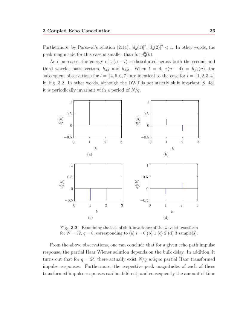
3.2 Examining the lack of shift invariance of the wavelet transform for
N = 32, q = 8, corresponding to (a) l = 0 (b) 1 (c) 2 (d) 3 sample(s). 36
3.3 Set of transformed impulse responses corresponding to m5(n). . . . . 37
3.4 Probability of correctly (Pc) estimating peak delays. . . . . . . . . . . 38
3.5 ITU-T G.168 hybrid impulse response. . . . . . . . . . . . . . . . . . 45
3.6 The mean-squared weight error plotted for three different partial Haar
adaptive filter lengths q = 256, 128, 64. . . . . . . . . . . . . . . . . . 46
4.1 Venn diagram representing the free DSm model. . . . . . . . . . . . . 57
4.2 Block diagram of peak discernibility measure (PDM) calculation. . . . 62
4.3 Linear piecewise membership functions derived from φs(x) and 1−φn(x)
(based on simulation). . . . . . . . . . . . . . . . . . . . . . . . . . . 64
4.4 A robust approximation of membership functions. . . . . . . . . . . . 64
4.5 Block diagram of Peak Tendency Estimator. . . . . . . . . . . . . . . 65
4.6 Peak-tendency estimation algorithm. . . . . . . . . . . . . . . . . . . 68
4.7 Suboptimal-Context Escape Algorithm. . . . . . . . . . . . . . . . . . 71
List of Figures viii
4.8 Improved tracking algorithm with suboptimal-context escaping. . . . 74
4.9 Multiple echo cancellation system architecture. . . . . . . . . . . . . . 75
4.10 Illustrating the difference between partitions and overlapping regions. 75
4.11 Multiple echo cancellation agent architecture. . . . . . . . . . . . . . 77
4.12 Multiple echo canceller. . . . . . . . . . . . . . . . . . . . . . . . . . . 78
5.1 ITU-T hybrid response m5(k) learning curves using a: (a) best and (b)
worst-case bulk delay for the initial context used. (SNR = 30 dB) . . 84
5.2 Learning curves over 1000 runs, with randomly-selected (equiprobable)
hybrid impulse responses and uniformly-selected bulk delays. (SNR
= 30 dB) . . . . . . . . . . . . . . . . . . . . . . . . . . . . . . . . . . 85
5.3 Tracking behaviour of the IT-PHDAF compared to the PHDAF and
NLMS algorithm: (a) Best-to-Best change in bulk delay for the initial
context used; (b) Worst-to-worst change in bulk delay. (SNR = 30 dB) 90
5.4 Tracking behaviour of the IT-PHDAF compared to the PHDAF and
NLMS algorithm: (a) Best-to-worst case change in bulk delay for the
initial context used; (b) Worst-to-best context change in bulk delay.
(SNR = 30 dB) . . . . . . . . . . . . . . . . . . . . . . . . . . . . . . 91
5.5 ITU-T hybrid response m5(k) learning curves using a multiple echo
canceller and the PHDAF: (a) best-case bulk delay; (b) worst-case
bulk delay. (SNR = 30 dB) . . . . . . . . . . . . . . . . . . . . . . . 96
5.6 (a) Learning curves over 600 runs using two random hybrid impulse
responses and random bulk delays (SNR = 30 dB); (b) Corresponding
percentage of dominant number of agents activated in 600 simulations. 97
5.7 (a) Learning curves over 1000 runs using three random hybrid impulse
responses and random bulk delays (SNR = 30 dB); (b) Corresponding
percentage of dominant number of agents activated in 1000 simulations. 98

ix
List of Tables
4.1 Fuzzy Rule Bases . . . . . . . . . . . . . . . . . . . . . . . . . . . . . 66
4.2 Fuzzy graphs corresponding to two models of peak behaviour. . . . . 67
5.1 Comparison of mean times and standard deviation to correctly estimate
the peak delay for different SNRs. . . . . . . . . . . . . . . . . . . . . 85
5.2 Number of arithmetic operations per iteration - single dispersive region 89
5.3 Number of arithmetic operations per iteration - multiple dispersive
regions . . . . . . . . . . . . . . . . . . . . . . . . . . . . . . . . . . . 95

x
List of Acronyms
CDF Cumulative Distribution Function
CWT Continuous Wavelet Transform
DMT Discrete Multitone Modulation
DST Dempster-Shafer Theory
DSmT Dezert-Smarandache Theory
DWT Discrete Wavelet Transform
ERL Echo Return Loss
FIR Finite Impulse Response
IT-PHDAF Improved Tracking Partial Haar Dual Adaptive Filter
ITU International Telecommunication Union
LMS Least Mean Square
LS Least Squares
LTI Linear Time Invariant
ME-PHDAF Multiple Echo Partial Haar Dual Adaptive Filter
MFLOPS Million Floating Point Operations per Second
MRA Multi-resolution Analysis
MSE Mean Squared Error
NLMS Normalized Least Mean Squares
PDM Peak Discernibility Measure
PDF Probability Density Function
PHDAF Partial Haar Dual Adaptive Filter
PNLMS Proportionate Normalized Least Mean Squares
PSTN Public Switched Telephone Network
RLS Recursive Least Squares

List of Terms xi
RDWT Redundant Discrete Wavelet Transform
SCE-PHDAF Suboptimal Context Escaping Partial Haar Dual Adaptive Filter
SNR Signal-to-Noise ratio
STWQ Scrub Taps Waiting in a Queue
VoIP Voice over Internet Protocol
1
Chapter 1
Introduction
This chapter is divided into four parts. First, the telephone network environment is
introduced as a backdrop to the problem of line echo and its implications. This is
followed by a review of sparse echo cancellers that have been developed over recent
years, including a specific echo canceller which will be the focus of this work. Section
1.3 discusses the scope of this research and the contributions made. The chapter
concludes with an overview of the subsequent chapters of this text.
1.1 Line Echo in Voice Communications
The presence of echo has been and is still commonplace in today’s ever-expanding
communication infrastructure. In a telephone call scenario, the echo phenomenon can
be described by a caller as hearing a duplicate of his or her voice delayed in time.
Depending on the delay of the duplicate signal, the echo can be characterized as nearly
imperceptible for small delays to obstructing conversations when the delay is longer.
The most well known occurrence of echo is in telephone networks. A user’s phone
is connected to the local exchange or local telephone company (also termed the central
office) via a twisted pair of copper wires called the subscriber loop, terminating in
a line circuit, that connects to the public-switched telephone network (PSTN) [41].
The line circuit includes a device called a hybrid that converts the twisted pair run-
ning from a user’s premises into a four-wire connection, where each pair of wires is
separately used for transmit and receive signals.
2006/09/28
1 Introduction 2
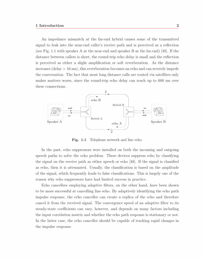
An impedance mismatch at the far-end hybrid causes some of the transmitted
signal to leak into the near-end caller’s receive path and is perceived as a reflection
(see Fig. 1.1 with speaker A at the near-end and speaker B at the far-end) [48]. If the
distance between callers is short, the round-trip echo delay is small and the reflection
is perceived as either a slight amplification or soft reverberation. As the distance
increases (delay > 16 ms), this reverberation becomes an echo and can severely impede
the conversation. The fact that most long distance calls are routed via satellites only
makes matters worse, since the round-trip echo delay can reach up to 600 ms over
these connections.
send
rec
rec
send
Speaker A Speaker BHybrid A
Hybrid B
echo B
echo A
2
2
Fig. 1.1 Telephone network and line echo.
In the past, echo suppressors were installed on both the incoming and outgoing
speech paths to solve the echo problem. These devices suppress echo by classifying
the signal on the receive path as either speech or echo [48]. If the signal is classified
as echo, then it is attenuated. Usually, the classification is based on the amplitude
of the signal, which frequently leads to false classifications. This is largely one of the
reason why echo suppressors have had limited success in practice.
Echo cancellers employing adaptive filters, on the other hand, have been shown
to be more successful at cancelling line echo. By adaptively identifying the echo path
impulse response, the echo canceller can create a replica of the echo and therefore
cancel it from the received signal. The convergence speed of an adaptive filter to its
steady-state coefficients can vary, however, and depends on many factors including
the input correlation matrix and whether the echo path response is stationary or not.
In the latter case, the echo canceller should be capable of tracking rapid changes in
the impulse response.
1 Introduction 3
Another hindrance to an echo canceller is double-talk, which occurs when both
users are speaking simultaneously. Double-talk corrupts the desired signal required to
cancel the echo, and negatively affects the steady-state mode of the adaptive filter’s
operation. Although it is not too common for people to be speaking simultaneously
during a phone call, the control logic should inhibit the echo canceller when double-
talk does occur. Double-talk detection will not be considered in this thesis.
An interesting fact about advancements in improving communication quality has
been an increase in the adverse effects of echo. By adding coders and signal processing
blocks into the line circuit, processing delays ranging from 80–100 ms have been
introduced into the round trip delay of echo [48]. Therefore, line echo that was
previously perceived as a slight amplification or reverberation can now be distinctly
heard as an echo. This byproduct of increased processing delays is making the effects
of echo even worse for Voice over Internet Protocol (VoIP) telephones, which are
deployed onto the existing telephone infrastructure. In addition to the processing
delays already present in the network, these telephones also require buffering delays
for the packetization of speech, not to mention delays resulting from the sharing of
network resources with other data packets [34]. One of the well known problems
encountered in VoIP is known as ‘initial echo’, which is echo experienced at the
beginning of a phone call, while the echo canceller is still converging, allowing the
reflection of residual echo back to the speaker [26].
In addition to affecting voice communications, echo also impedes the introduction
of transmission methods such as discrete multitone modulation (DMT), which divides
the transmission channel into a set of orthogonal subchannels [9, 25]. Echo cancella-
tion is usually not necessary when different sets of subchannels are used for up- and
down-links. However, full-duplex transmission, which can significantly increase the
obtainable data rates, requires echo cancellation.
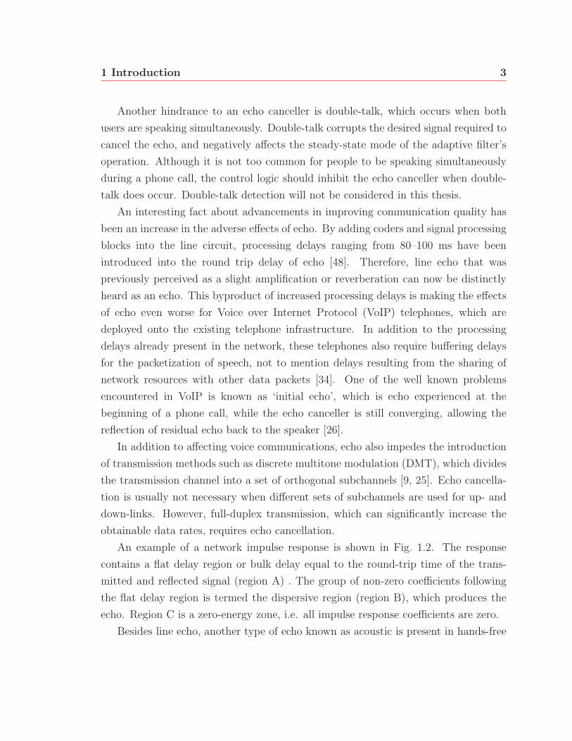
An example of a network impulse response is shown in Fig. 1.2. The response
contains a flat delay region or bulk delay equal to the round-trip time of the trans-
mitted and reflected signal (region A) . The group of non-zero coefficients following
the flat delay region is termed the dispersive region (region B), which produces the
echo. Region C is a zero-energy zone, i.e. all impulse response coefficients are zero.
Besides line echo, another type of echo known as acoustic is present in hands-free
1 Introduction 4
0
0
0.05
−0.05
0.1
100 200 300 400 500
A B C
samples
Fig. 1.2 Typical network impulse response.
communication. This echo results from the multiple reflections of sound emitted by
the loudspeaker (in three-dimensional space), which reach a microphone with differ-
ent delays [7]. Unlike acoustic echo, network or line echo involves specific reflection
points (impedance mismatches) placed over longer distances, along a one-dimensional
transmission medium. This makes echo path impulse responses in networks inherently
sparse compared to acoustic echo.
Although both types of echo affect telephone conversations, this thesis will only
be concerned with line echo. The main focus of this work will be based on an efficient
and fast echo canceller that takes advantage of the sparse characteristic of echo path
impulse responses in telephone networks.
1.2 Literature Review
The literature abounds with adaptive filtering algorithms that exploit the sparse char-
acteristics of line echo [33]. Most algorithms are based on finding ways to determine
which filter coefficients are actually associated with the echo, and then adapting only
these coefficients.
One of the earliest works on sparse echo cancellation is by Duttweiler [16], where
the input and desired signals are bandpass-filtered and decimated, and used by a
short (i.e. small number of coefficients) adaptive filter to locate the impulse response’s
dispersive region. If D is the decimation factor, then this approach requires only 1/D
as many taps as a traditional echo canceller. A shorter filter operating at the original
sampling rate is then centred around the dispersive region to cancel the echo. Using
this approach, only two short adaptive filters are required, compared to one long

1 Introduction 5
filter, reducing complexity and increasing convergence speed. However, Duttweiler’s
echo canceller suffers from many drawbacks as remarked by [4]. The most obvious
drawback stems from the observation that the convergence time of the echo canceller
depends on the decimated adaptive filter, which is operating D-times slower than the
rate of incoming data. Therefore, the time required to correctly estimate the delay
can be quite long. Secondly, in speech applications, the bandlimiting operation can
remove important frequency components in the signals, preventing proper convergence
of the subsampled adaptive filter.
An adaptive multiple echo canceller is proposed in [50]. It uses a full-length pri-
mary adaptive filter in parallel with a group of short secondary adaptive filters. A
monitor/control unit switches between the output of these two classes of filters, de-
pending on specific conditions. The full-length filter is used to track multiple dis-
persive regions and initially cancels echo, while each short adaptive filter is centred
around these regions once the full-length filter has sufficiently converged. One of the
biggest problems with this approach is the added complexity of the monitor/control
unit, in addition to the extra hardware and power requirements of a full length adap-
tive filter.
In [46], an algorithm based on the so-called “Scrub Taps Waiting in a Queue”
(STWQ) approach [27] for sparse channel impulse responses is proposed that uses a
two-stage adaptation process. The first part of the process estimates the flat delay
region, and the second part consists of adapting those filter coefficients using a con-
strained tap-position control. This constrained control puts a limit on which filter
taps can be updated based on their relative position within the dispersive region.
Probably one of the most well-known class of sparse echo cancellers are based
on the Proportionate Normalized Least Mean Squares (PNLMS) algorithm [17] and
its ubiquitous variants. These include the improved PNLMS (IPNLMS) [3], the
PNLMS++ [19], and the improved IPNLMS [11]. These algorithms allocate individ-
ual step-size gains in proportion to the magnitude of each filter coefficient. Therefore,
coefficients with large magnitudes converge quickly to their steady-state values, while
coefficients in the flat delay region that would normally only contribute to tap-weight
noise are updated using very small step-sizes. The only drawbacks of this algorithm
are its increased computational complexity and its degradation in performance as the

1 Introduction 6
length and/or number of dispersive regions increases.
Other attempts at improving sparse echo cancellation rely on using orthogonal
transforms such as the wavelet transform on the input data. In [24], the authors
propose using a subset of Haar wavelet coefficients to detect the significant channel
coefficients. Then, by exploiting the hierarchical structure of the dyadic wavelet
expansion, the locations of these significant coefficients are used to activate coefficients
in the remaining subsets that share the same non-zero time-support. Therefore, only
significant filter coefficients are adapted, increasing convergence speed and reducing
computational complexity.
More recently, Bershad and Bist [4] have proposed a novel way of cancelling sparse
echo, using a coupled echo canceller consisting of two short adaptive filters similar
to Duttweiler’s approach [16]. The first partial Haar filter operates on only a subset
of input Haar coefficients, and is used by a peak delay estimator to determine the
location of the echo path’s dispersive region. Unlike Duttweiler’s echo canceller [16]
which requires the design of complex bandpass filters, the Haar wavelet transform is
simpler and just as amenable to digital signal processors. The second time-domain
filter is then centred around this location to actually cancel the echo. In cases where
the bulk delay is very large and a traditional echo canceller would require a large
number of taps, this new method provides a significant reduction in computation and
memory requirements. Most importantly, by reducing the number of filter taps, the
convergence speed of the overall echo canceller is increased.
1.3 Research Objectives and Contribution
Although some of the previously-mentioned sparse adaptive filtering algorithms have
shown promising results, the coupled echo canceller proposed by Bershad and Bist [4]
uses a more novel method of incorporating channel-monitoring for sparse echo can-
cellation. Because channel-monitoring is performed in parallel with the actual echo
cancellation process, this can provide greater flexibility from a researcher’s point of
view in experimenting with new ideas to improve the overall echo canceller. With its
significant increase in convergence speed and reduced complexity, the coupled echo
canceller still suffers from a few drawbacks, however.
1 Introduction 7
First, the shift-variant property of wavelet transforms makes the performance of
the partial Haar adaptive filter highly dependent on the echo path bulk delay. As
a result, the specific value of the bulk delay can affect the amount of time it takes
the peak delay estimator to correctly estimate the location of the dispersive region,
significantly affecting the overall convergence speed of the echo canceller.
Second, the promising results shown by [4] that support the increased convergence
speed are only valid for stationary channels. The reason for this is the simulations
that produced these results assume that the filter taps are initially set to zero. In
non-stationary environments, where the bulk delay of the echo path impulse response
can abruptly change, the amount of time required by the peak delay estimator to
locate new dispersive regions can be very large.
Finally, the coupled echo canceller has only been analyzed and developed for the
case of a single dispersive region. In today’s communication networks, interfaces
between different transmission media such as copper to fibre optic cables can also
produce unwanted echo [48]. Consequently, it is not uncommon for an echo path im-
pulse response to contain multiple dispersive regions. It would therefore be necessary
to modify the original coupled echo canceller [4] to accommodate multiple echoes.
In addition to some implementation issues, this thesis looks at the above problems,
and investigates possible solutions for each. More specifically,
- To deal with the shift-variant property of wavelet transforms, a peak tendency
estimator is proposed that is based on non-Bayesian evidence theory and fuzzy
inference. The estimator categorizes a peak’s magnitude behaviour as either
increasing or decreasing. When the current peak is categorized as decreasing
and displaying jitter, then a different set of transformed input coefficients is
used to drive the partial Haar adaptive filter to a Wiener solution with a larger
peak. Deciding when to use a different transformed input vector is based on a
schedule of trial periods.
- The proposed peak tendency estimator is also used to improve the tracking
performance of the coupled echo canceller in situations where an abrupt change
in an echo path impulse response’s bulk delay occurs. Because the partial Haar
adaptive filter is not cancelling echo directly, it can be reset to zero whenever a
1 Introduction 8
change in bulk delay is detected as a decrease in the current peak magnitude.
The old peak position is used to offset the short time-domain filter until a new
peak has been found. As Bershad and Bist have shown [4], the peak delay
estimator usually locates peaks faster when the partial Haar adaptive filter is
reset to zero.
- A multiple echo canceller similar to [50] is proposed that assigns multiple agents
to overlapping regions of the partial Haar adaptive filter, with each agent per-
forming peak tendency estimation. When true peaks are found, their locations
are relayed to a central coordinator that activates or deactivates the coefficients
of a full-length time-domain filter used to cancel echo.
The performance gains of the above contributions are supported by simulation. Each
contribution to the echo canceller is tested using ITU-T G.168 [1] hybrid impulse
responses. The simulations are divided into two classes and range from specific test-
scenarios to randomly generated cases. Each class of tests is required to understand
the proposed algorithms in detail while at the same time establishing their perfor-
mance in general. It is shown that each of the proposed solutions can substantially
improve the coupled echo canceller’s performance.
1.4 Thesis Overview
This text is organized as follows: Chapter 2 begins with an overview of wavelets and
adaptive filtering theory. The aim of this chapter is to focus and narrow the breadth
of these fields within the scope of the coupled echo canceller.
Chapter 3 provides the analysis of the coupled echo canceller proposed by Bershad
and Bist [4], followed by an in depth critique of the different problems associated with
this echo canceller.
Proposed solutions to these problems are developed in Chapter 4. These include
ways of mitigating the effects of shift variance, improved tracking of abrupt changes
in bulk delays, and extending the echo canceller to accommodate multiple dispersive
regions.
Chapter 5 provides a series of simulation experiments to justify the advantages of

1 Introduction 9
the proposed solutions. These simulations are accompanied by discussions pertaining
to the results.
Finally, Chapter 6 concludes the text with a brief summary of the work, in addition
to possible future work and improvements to the proposed algorithms.

10
Chapter 2
Background
This chapter provides the theoretical background necessary to understand the ensuing
discussion in Chapter 3 of the coupled algorithm proposed by Bershad and Bist [4].
Because the coupled algorithm makes use of the Haar transform, the first section
provides a brief introduction to wavelets. The second section discusses basic adaptive
filtering theory, with particular emphasis on the LMS and NLMS algorithms.
2.1 A Brief Introduction to Wavelets
The theory of wavelets and their mathematical formulation have been well established
since the early 1900s [8]. However, it has only been after the advent of improved
processing power that the full potential and flexibility of wavelets have been realized
in digital signal processing. In fact, one of the first algorithms utilizing wavelets for
signal analysis dates back to the work of Stephane Mallat [32] in the 1980s.
Wavelets can be viewed as functions that obey certain mathematical constraints
to represent other functions (signals). In addition to the time-frequency descriptive
provided by wavelet transforms, these mathematical constraints also make possible the
notion of multiresolution analysis. In other words, by properly scaling (i.e. dilating
or contracting) and shifting a wavelet function along the time-axis, it is possible to
describe the same signal with varying degrees of detail.
Unlike the class of Fourier expansions that decompose a signal in terms of sinusoids
with infinite time-support, wavelet functions are not restricted to any one class of basis
2006/09/28
2 Background 11
functions, and also include functions with finite time-support. This makes it possible
to construct wavelet functions to obtain signal representations that are sparse or that
emphasize certain desired properties of a signal [38]. Wavelet transforms also provide
a dual time-frequency description of a signal which is absent from Fourier analysis.
Applications of wavelets in signal processing are seemingly endless, and include
image processing, time-series analysis, sound synthesis, and data compression [21]. In
applications such as image denoising, an image is decomposed into a set of wavelet
coefficients, and those coefficients with magnitudes less than a specified threshold
are set to zero. A denoised version is then constructed using the inverse wavelet
transform of the resulting coefficients. Wavelets enjoy even more widespread use in
data compression, where their sparse representations allow the storage of a signal’s
information in very few coefficients [38].
The following section discusses the fundamentals of wavelets and their properties.
This discussion is limited to the Discrete Wavelet Transform (DWT), since its analysis
leads to practical and efficient applications in digital signal processing.
2.1.1 Discrete Wavelet Transform
The DWT arose from a necessity to overcome some of the inherent difficulties associ-
ated with the Continuous Wavelet Transform (CWT) [31]. These difficulties include
redundancy, and an uncountable number of wavelets resulting from continuous scaling
and translation variables. More importantly, however, the CWT does not lend itself to
any fast algorithms for computing the transform [31]. Although discrete wavelets are
continuous functions of time, they can only be scaled and translated in discrete steps,
such as the dyadic DWT which uses scaling steps of size 2 and will be considered here.
A. Scaling Function
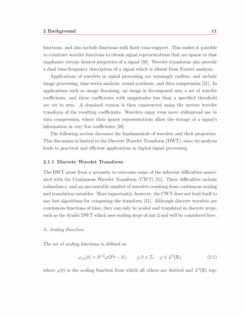
The set of scaling functions is defined as
ϕj,k(t) = 2j/2ϕ(2jt− k), j, k ∈ Z, ϕ ∈ L2(R), (2.1)
where ϕ(t) is the scaling function from which all others are derived and L2(R) rep-
2 Background 12
resents the set of functions (of real variables) with well-defined square integrals [8].
This function has two properties. First, it is scalable in time (2jt term), and second,
at each scale, the set of functions include integer-translates k of ϕ(2jt). A small scale
index j corresponds to a coarse time-resolution, while a large scale index reflects finer
time-resolution1. In addition, for the sake of simplicity, the scale index j will only
assume non-negative values. The set of scaling functions is two-dimensional, as it
represents a given localization in time determined by k at a given scale index j, hence
the term time-frequency resolution associated with wavelets.
The time support of the function ϕ(t) is usually normalized to the interval [0, 1).
As a result, the value of k ranges from 0 to 2j − 1. As the scale index increases (finer
time resolution), the number of possible translations increases exponentially. At a
given scale index j, the subspace spanned by these functions over translations k is
denoted by
Vj = span{ϕj,k(t)}. (2.2)
Multiresolution analysis is made possible by requiring that
Vj ⊂ Vj+1. (2.3)
This means that those coefficients generated by expanding a signal at a coarser scale
can be constructed from coefficients at a finer scale. The expression that relates the
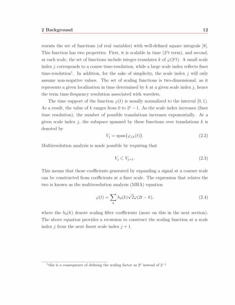
two is known as the multiresolution analysis (MRA) equation
ϕ(t) =∑
k
h0(k)√
2ϕ(2t− k), (2.4)
where the h0(k) denote scaling filter coefficients (more on this in the next section).
The above equation provides a recursion to construct the scaling function at a scale
index j from the next finest scale index j + 1.
1this is a consequence of defining the scaling factor as 2j instead of 2−j

2 Background 13
B. Wavelet Function
The wavelet function is given by
ψj,k(t) = 2j/2ψ(2jt− k), j, k ∈ Z, (2.5)
where ψ(t) is known as the mother wavelet, and the variables j and k again represent
the scale and translation indices, respectively. At a given scale index j, the subspace
spanned by these wavelet functions is denoted by
Wj = span{ψj,k(t)}. (2.6)
The set of wavelet functions span the differences between the spaces spanned by
successive scaling functions ϕ(2jt) and ϕ(2j+1t). By construction, this space is related
to Vj, and satisfies the following condition,
Vj+1 = Vj ⊕Wj, (2.7)
where ⊕ denotes a direct sum of subspaces. Equation (2.7) implies that
Vj = V0 ⊕W0 ⊕W1 ⊕ · · · ⊕Wj−1. (2.8)
Furthermore, one can conclude that in order to span Vj the initial subspace Vj0 can
have an arbitrary scale 0 ≤ j0 < j. Therefore, Vj is can also be represented by
Vj = Vj0 ⊕Wj0 ⊕Wj0+1 ⊕ · · · ⊕Wj−1. (2.9)
This makes sense intuitively because from (2.7), the span of the initial scaling functions
contain the spans of all the scaling functions with scale indices less than j0, i.e.
V0 ⊂ V1 ⊂ · · · ⊂ Vj0 . (2.10)
As a result of (2.7) and (2.9), any function g(t) ∈ L2(R) can be written as a sum of
2 Background 14
time-shifted versions of an arbitrary scaling function and a set of wavelet functions,
g(t) =∑
k
cj0(k)ϕj0,k(t) +∞∑
j=j0
∑k
dj(k)ψj,k(t), (2.11)
where cj(k) and dj(k) are the scaling and wavelet (or difference) coefficients, respec-
tively. To make the calculation of the wavelet coefficients tractable, an important
requirement is for the wavelet and scaling functions to be orthogonal,
〈ϕj,k(t), ψj,l(t)〉 =
∫ϕj,k(t)ψj,l(t)dt = 0, ∀j, k �= l ∈ Z (2.12)
and for the wavelet functions, whether at the same or different scale, to be orthogonal
〈ψj,k(t), ψj′,l(t)〉 =
∫ψj,k(t)ψj′,l(t)dt = 0,
∀j = j′, k �= l ∈ Z
∀(j, k) �= (j′, l) ∈ Z2
(2.13)
Furthermore, if the scaling and wavelet functions have unit norm in addition to the
conditions in (2.12) and (2.13), then Parseval’s relation holds true for the DWT, i.e.∫|g(t)|2dt =
∑k
|cj0(k)|2 +∞∑
j=j0
∑k
|dj(k)|2. (2.14)
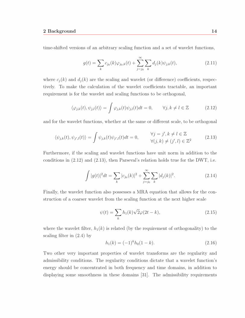
Finally, the wavelet function also possesses a MRA equation that allows for the con-
struction of a coarser wavelet from the scaling function at the next higher scale
ψ(t) =∑
k
h1(k)√
2ϕ(2t− k), (2.15)
where the wavelet filter, h1(k) is related (by the requirement of orthogonality) to the
scaling filter in (2.4) by
h1(k) = (−1)kh0(1 − k). (2.16)
Two other very important properties of wavelet transforms are the regularity and
admissibility conditions. The regularity conditions dictate that a wavelet function’s
energy should be concentrated in both frequency and time domains, in addition to
displaying some smoothness in these domains [31]. The admissibility requirements

2 Background 15
state that the Fourier transform of the wavelet function is zero at the zero frequency
(the time average of the wavelet function is zero). From a spectral perspective then,
it is now apparent why scaling functions are used in conjunction with wavelets. Scal-
ing functions fill in the low-frequency ‘spectral gap’ resulting form the admissibility
conditions (an admissibility condition for scaling functions requires that their zero-
moment be non-zero). Otherwise, filling this spectral gap could only be achieved in
the limit of an infinite number of wavelet functions [31]. Therefore, wavelet functions
can be seen as band-pass filters while scaling functions correspond to low-pass filters.
Of course, all these constraints are meaningless unless there actually exists a set
of scaling and wavelet functions that satisfy the above constraints. The next section
introduces the Haar wavelet and its corresponding scaling function. Both functions
are probably the most basic of all wavelet/scaling functions.
2.1.2 An Example: The Haar Wavelet
The Haar wavelet, introduced by Alfred Haar in his 1909 thesis, is probably the most
basic of all wavelets [8]. The scaling and wavelet functions consist of shifted and
scaled versions of a square wave. The functions ϕ(t) and ψ(t) are shown in Fig. 2.1
normalized to the interval [0, 1). The equations for each are
ϕ(t) =
{1, t ∈ [0, 1)
0, t /∈ [0, 1)ψ(t) =
⎧⎪⎨⎪⎩1, t ∈ [0, 1/2)
−1, t ∈ [1/2, 1)
0, t /∈ [0, 1)
(2.17)
t0
1
1
(a)
t
1
1
− 1
0
(b)
Fig. 2.1 Haar (a) scaling and (b) wavelet functions.
2 Background 16
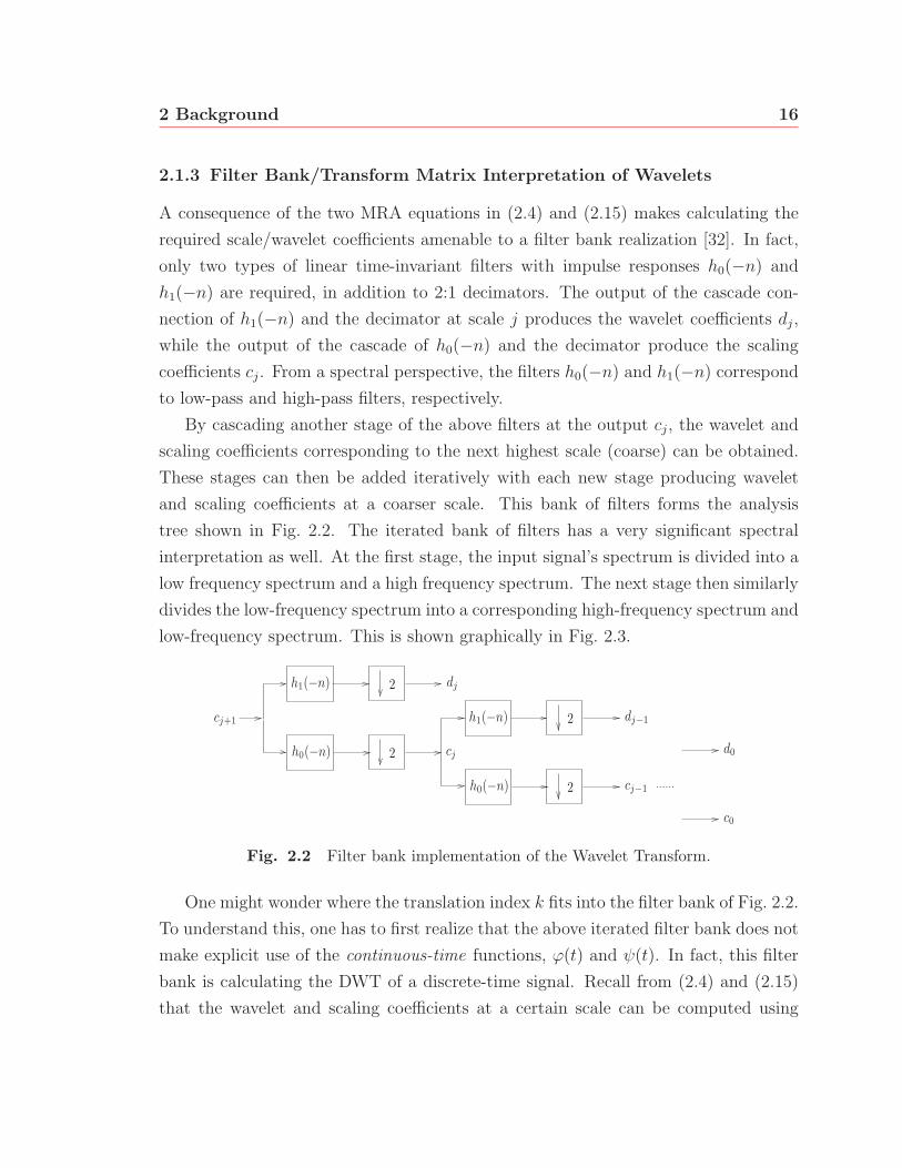
2.1.3 Filter Bank/Transform Matrix Interpretation of Wavelets
A consequence of the two MRA equations in (2.4) and (2.15) makes calculating the
required scale/wavelet coefficients amenable to a filter bank realization [32]. In fact,
only two types of linear time-invariant filters with impulse responses h0(−n) and
h1(−n) are required, in addition to 2:1 decimators. The output of the cascade con-
nection of h1(−n) and the decimator at scale j produces the wavelet coefficients dj,
while the output of the cascade of h0(−n) and the decimator produce the scaling
coefficients cj. From a spectral perspective, the filters h0(−n) and h1(−n) correspond
to low-pass and high-pass filters, respectively.
By cascading another stage of the above filters at the output cj, the wavelet and
scaling coefficients corresponding to the next highest scale (coarse) can be obtained.
These stages can then be added iteratively with each new stage producing wavelet
and scaling coefficients at a coarser scale. This bank of filters forms the analysis
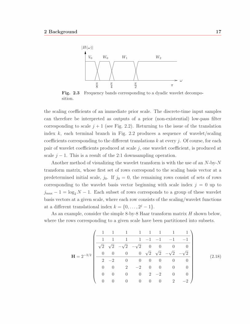
tree shown in Fig. 2.2. The iterated bank of filters has a very significant spectral
interpretation as well. At the first stage, the input signal’s spectrum is divided into a
low frequency spectrum and a high frequency spectrum. The next stage then similarly
divides the low-frequency spectrum into a corresponding high-frequency spectrum and
low-frequency spectrum. This is shown graphically in Fig. 2.3.
cj+1
h0(−n)
h0(−n)
h1(−n)
h1(−n)
2
2
2
2
dj
cj
dj−1
cj−1
d0
c0
Fig. 2.2 Filter bank implementation of the Wavelet Transform.
One might wonder where the translation index k fits into the filter bank of Fig. 2.2.
To understand this, one has to first realize that the above iterated filter bank does not
make explicit use of the continuous-time functions, ϕ(t) and ψ(t). In fact, this filter
bank is calculating the DWT of a discrete-time signal. Recall from (2.4) and (2.15)
that the wavelet and scaling coefficients at a certain scale can be computed using
2 Background 17
ππ2
π4
π8
ω
V0 W0 W1 W2
|H(ω)|
Fig. 2.3 Frequency bands corresponding to a dyadic wavelet decompo-sition.
the scaling coefficients of an immediate prior scale. The discrete-time input samples
can therefore be interpreted as outputs of a prior (non-existential) low-pass filter
corresponding to scale j + 1 (see Fig. 2.2). Returning to the issue of the translation
index k, each terminal branch in Fig. 2.2 produces a sequence of wavelet/scaling
coefficients corresponding to the different translations k at every j. Of course, for each
pair of wavelet coefficients produced at scale j, one wavelet coefficient, is produced at
scale j − 1. This is a result of the 2:1 downsampling operation.
Another method of visualizing the wavelet transform is with the use of an N -by-N
transform matrix, whose first set of rows correspond to the scaling basis vector at a
predetermined initial scale, j0. If j0 = 0, the remaining rows consist of sets of rows
corresponding to the wavelet basis vector beginning with scale index j = 0 up to
jmax − 1 = log2N − 1. Each subset of rows corresponds to a group of these wavelet
basis vectors at a given scale, where each row consists of the scaling/wavelet functions
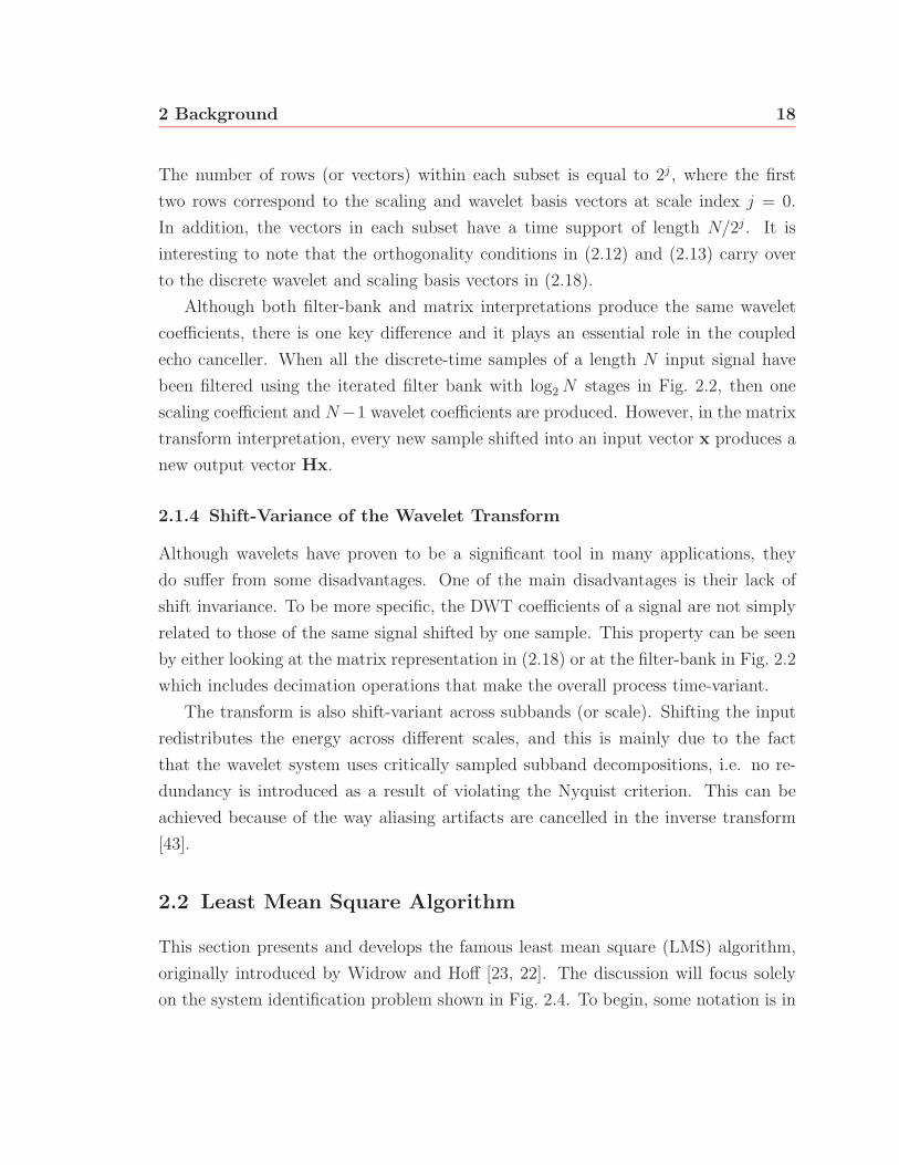
at a different translational index k = {0, . . . , 2j − 1}.As an example, consider the simple 8-by-8 Haar transform matrix H shown below,
where the rows corresponding to a given scale have been partitioned into subsets.
H = 2−3/2
⎛⎜⎜⎜⎜⎜⎜⎜⎜⎜⎜⎜⎜⎜⎜⎝
1 1 1 1 1 1 1 1
1 1 1 1 −1 −1 −1 −1√2
√2 −√
2 −√2 0 0 0 0
0 0 0 0√
2√
2 −√2 −√
2
2 −2 0 0 0 0 0 0
0 0 2 −2 0 0 0 0
0 0 0 0 2 −2 0 0
0 0 0 0 0 0 2 −2
⎞⎟⎟⎟⎟⎟⎟⎟⎟⎟⎟⎟⎟⎟⎟⎠(2.18)
2 Background 18
The number of rows (or vectors) within each subset is equal to 2j, where the first
two rows correspond to the scaling and wavelet basis vectors at scale index j = 0.
In addition, the vectors in each subset have a time support of length N/2j. It is
interesting to note that the orthogonality conditions in (2.12) and (2.13) carry over
to the discrete wavelet and scaling basis vectors in (2.18).
Although both filter-bank and matrix interpretations produce the same wavelet
coefficients, there is one key difference and it plays an essential role in the coupled
echo canceller. When all the discrete-time samples of a length N input signal have
been filtered using the iterated filter bank with log2N stages in Fig. 2.2, then one
scaling coefficient and N−1 wavelet coefficients are produced. However, in the matrix
transform interpretation, every new sample shifted into an input vector x produces a
new output vector Hx.
2.1.4 Shift-Variance of the Wavelet Transform
Although wavelets have proven to be a significant tool in many applications, they
do suffer from some disadvantages. One of the main disadvantages is their lack of
shift invariance. To be more specific, the DWT coefficients of a signal are not simply
related to those of the same signal shifted by one sample. This property can be seen
by either looking at the matrix representation in (2.18) or at the filter-bank in Fig. 2.2
which includes decimation operations that make the overall process time-variant.
The transform is also shift-variant across subbands (or scale). Shifting the input
redistributes the energy across different scales, and this is mainly due to the fact
that the wavelet system uses critically sampled subband decompositions, i.e. no re-
dundancy is introduced as a result of violating the Nyquist criterion. This can be
achieved because of the way aliasing artifacts are cancelled in the inverse transform
[43].
2.2 Least Mean Square Algorithm
This section presents and develops the famous least mean square (LMS) algorithm,
originally introduced by Widrow and Hoff [23, 22]. The discussion will focus solely
on the system identification problem shown in Fig. 2.4. To begin, some notation is in
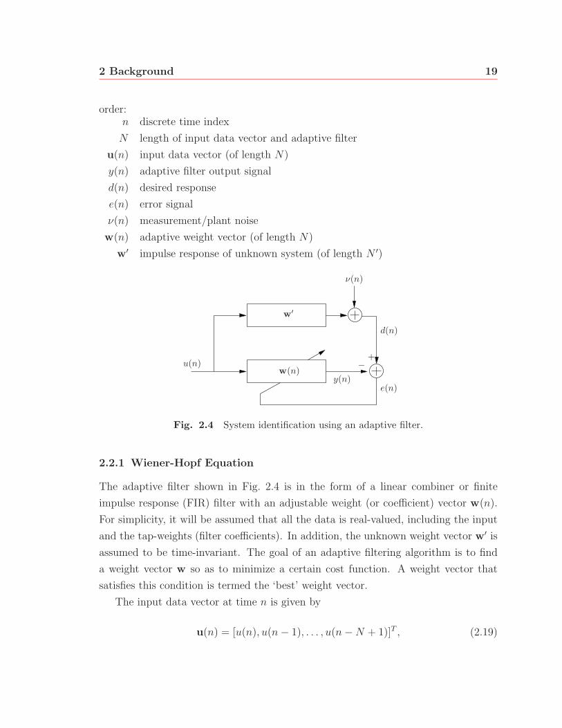
2 Background 19
order:n discrete time index
N length of input data vector and adaptive filter
u(n) input data vector (of length N)
y(n) adaptive filter output signal
d(n) desired response
e(n) error signal
ν(n) measurement/plant noise
w(n) adaptive weight vector (of length N)
w′ impulse response of unknown system (of length N ′)
u(n)
y(n)
−+
e(n)
ν(n)
d(n)
w(n)
w′
Fig. 2.4 System identification using an adaptive filter.
2.2.1 Wiener-Hopf Equation
The adaptive filter shown in Fig. 2.4 is in the form of a linear combiner or finite
impulse response (FIR) filter with an adjustable weight (or coefficient) vector w(n).
For simplicity, it will be assumed that all the data is real-valued, including the input
and the tap-weights (filter coefficients). In addition, the unknown weight vector w′ is
assumed to be time-invariant. The goal of an adaptive filtering algorithm is to find
a weight vector w so as to minimize a certain cost function. A weight vector that
satisfies this condition is termed the ‘best’ weight vector.
The input data vector at time n is given by
u(n) = [u(n), u(n− 1), . . . , u(n−N + 1)]T , (2.19)
2 Background 20
and the weight vector is denoted by
w = [w1, w2, . . . , wN ]T . (2.20)
Each input sample is multiplied with its respective tap-weight, and the results are
added to produce the output
y(n) = wTu(n) =N∑
k=1
wku(n− k + 1). (2.21)
The error at time n is
e(n) = d(n) − y(n) = d(n) − wTu(n), (2.22)
where
d(n) = w′Tu(n) + ν(n) (2.23)
is the output to the true system (also called the plant) to be identified by the adapta-
tion process plus an additional term that can be attributed to plant or measurement
noise denoted by ν(n), assumed to be independent of u(n).
Here, the cost function to be minimized by the best weight vector is the mean
squared error (MSE),
J = E[e2(n)]
= E[d2(n) − 2d(n)wTu(n) + wTu(n)uT (n)w]
= σ2d − 2wTp + wTRw (2.24)
where σ2d denotes the variance of the desired response d(n), p = E[d(n)u(n)] is the
cross-correlation between the input data vector and the desired signal, and R =
E[u(n)uT (n)] is the input autocorrelation matrix. The above equation shows that
the MSE is a quadratic function of the tap-weight vector, w. Assuming that R > 0,
this implies that J(w) exhibits a unique minimum which can be found by following
the negative gradient of J(w) with respect to w. Differentiating (2.24) with respect
2 Background 21
to w,∂J(w)
∂w= −2p + 2Rw, (2.25)
and setting the result to zero, the famous Wiener-Hopf equation is obtained for the
optimal filter weights,
wo = R−1p. (2.26)
If N ≥ N ′, it can be shown that the Wiener solution wo corresponds to the true
weight vector of the unknown system w′ padded with N−N ′ zeros, i.e. wo = [w′T0]T .
In the sequel, it will be assumed that this condition is satisfied and the adaptive filter
length is sufficient to model w′, so that the symbol w′ can be replaced by wo.
When R is nonsingular (as is usually the case), the MSE expression in (2.24) can
be written as
J(w) = σ2d − pTR−1p + (w − R−1p)TR(w − R−1p). (2.27)
Therefore,
Jmin = minw
J(w) = σ2d − pTR−1p (2.28)
is satisfied for w = wo = R−1p. Expanding σ2d,
σ2d = E[d2(n)]
= E[(wTo u(n) + ν(n))2]
= σ2ν + wT
o Rwo, (2.29)
where σ2ν is the noise power and the independence of ν(n) and u(n) has been assumed.
Therefore (2.28) becomes
Jmin = σ2ν + wT
o Rwo − pTR−1p
= σ2ν . (2.30)
In the ideal case, at least, the minimum MSE reduces to the measurement noise power.

2 Background 22
In general then, (2.24) can be written as
J(w) = Jmin + (w − wo)TR(w − wo). (2.31)
2.2.2 LMS Algorithm
The LMS algorithm is based on the steepest-descent algorithm [22],
w(n+ 1) = w(n) − 1
2μ∂J(n)
∂w(n), (2.32)
where the tap-weights are now a function of time. Substituting (2.25) in (2.32), one
obtains the steepest descent algorithm’s update equation,
w(n+ 1) = w(n) + μ[p − Rw(n)]. (2.33)
Note that this is a deterministic equation since the quantities p and R are produced
by expectation operators.
The LMS algorithm on the other hand, approximates p and R with their instan-
taneous estimated values. As a result, the LMS update equation is given by
w(n+ 1) = w(n) + μ[d(n)u(n) − u(n)uT (n)w(n)]
= w(n) + μu(n)[d(n) − uT (n)w(n)]
= w(n) + μu(n)e(n). (2.34)
Because instantaneous, and therefore random values of the quantities p and R are
used, the LMS algorithms is a stochastic gradient algorithm.
2.2.3 Properties of the LMS Algorithm
Although the recursive form of the LMS filter in (2.34) is straightforward, its con-
vergence analysis is quite complicated (convergence usually refers to the behaviour of
the adaptive filter as it reaches its optimum solution). This can be seen by finding
2 Background 23
the closed-form expression of (2.34), assuming w(0) = 0,
w(n) = μn−1∑i=0
e(i)u(i). (2.35)
The filter output y(n) can then be written as
y(n) = wT (n)u(n)
= μn−1∑i=0
e(i)uT (i)u(n), (2.36)
where it is clear that y(n) is a non-linear function of the input vectors u(j), (j =
0, 1, . . . , n). The most common form of analysis of the LMS algorithm is based on
small step-size theory [22] which approximates the LMS weight error vector ε(n) =
wo − w(n), and its corresponding recursion
ε(n+ 1) = [I − μu(n)uT (n)]ε(n) − μu(n)eo(n), (2.37)
with its zero-order recursion
ε0(n+ 1) = (I − μR)ε0(n) + f0(n), (2.38)
where eo(n) = d(n) − wTo u(n), is the output error corresponding to the Wiener so-
lution, and I is an N -by-N identity matrix. The second term in (2.37), f0(n) =
−μu(n)eo(n), is called the driving force. The eigendecomposition of the input correla-
tion matrix R is given by R = QΛQH , where Λ is the diagonal matrix of eigenvalues,
and Q is an orthogonal matrix of the respective eigenvectors. The transformed weight
error vector b(n) = QT ε0(n) consists of scalar entries known as the natural modes of
the filter. The transformed recursion in (2.38) becomes
b(n+ 1) = (I − μΛ)b(n) + φ(n), (2.39)
2 Background 24
where φ(n) = QT f0(n). If b(n+ 1) is decomposed into its individual components, bk,
then the expression for the kth natural mode is,
bk(n+ 1) = (1 − μλk)bk(n) + φk(n). (2.40)
A closed-form equation can be derived,
bk(n) = (1 − μλk)nbk(0) +
n−1∑i=0
(1 − μλk)n−i−1φk(i), (2.41)
whose mean value and mean squared value are
E[bk(n)] = bk(0)(1 − μλk)n (2.42)
E[|bk(n)|2] =μJmin
2 − μλk
+ (1 − μλk)2n(|bk(0)|2 − μJmin
2 − μλk
), (2.43)
respectively [22]. From this expression, one can determine the range of values of the
step-size μ so that the mean value of the natural modes decay to zero,
−1 < 1 − μλk < +1, ∀k. (2.44)
The corresponding range for μ is
0 < μ <2
λmax
, (2.45)
where λmax and λmin correspond to the maximum and minimum eigenvalues, respec-
tively. The average time constant of the LMS is a useful indicator of the convergence
time of the algorithm. The constant is derived from the average eigenvalue, defined
as λav = 1N
∑Nk=1 λk, and is given by
τav ≈ 1
2μλav
. (2.46)
For the steepest descent case, this time constant defines the amount of time it takes
on average for a natural mode to decay to 1/e of its initial value, bk(0). In fact, it can

2 Background 25
be shown [22] that the time constant τ of the filter ranges from
−1
ln(1 − μλmax)≤ τ ≤ −1
ln(1 − μλmin). (2.47)
As a result, the convergence time of the LMS algorithm is a function of the eigenspread
(also known as the condition number), λmax/λmin of the input autocorrelation R.
To derive an MSE equation similar to (2.31) within the context of the LMS algo-
rithm, w is replaced by a time-varying form w(n). Applying the eigenvalue decom-
position R = QΛQH , the expected value of the squared error, given w(n), is
E[e2(n)|w(n)] = Jmin +N∑
k=1
λk|bk(n)|2. (2.48)
The above equation, however, is stochastic because it depends on the random quan-
tities bk(n), (k = 1, 2, . . . , N). In order to obtain an expression for the mean square
error, the expectation of (2.48) is taken with respect to w(n) resulting in the expres-
sion
J(n) ≈ Jmin + tr[RK0(n)]
≈ Jmin +N∑
k=1
λkE[|bk(n)|2], (2.49)
where K0(n) = E[ε0(n)εT0 (n)] is the correlation matrix of the zero-order weight error
vector and using (2.43), the steady-state MSE is given by
J(∞) ≈ Jmin
(1 +
μ
2
N∑k=1
λk
). (2.50)
In the steepest descent case, where the driving force φ(n) is absent from the natural
mode recursion [22], the MSE in (2.48) decays to Jmin as the modes decay to zero.
However, the stochastic nature of the LMS produces a larger steady-state MSE, as
shown in the above equation.
2 Background 26
2.2.4 Normalized LMS Algorithm
One of the drawbacks of the LMS algorithm is gradient noise amplification. From
(2.34), the direction and magnitude of the tap update vector μu(n)e(n) is proportional
to the input data vector u(n) [22]. Therefore, any large increase in u(n) causes an
undesirable increase in the LMS update equation (2.34).
To overcome this problem, the normalized LMS algorithm (NLMS) normalizes the
weight update term in (2.34) by ||u(n)||2,
w(n+ 1) = w(n) +μ
‖u(n)‖2u(n)e(n). (2.51)
The above equation satisfies the principle of minimal disturbance [22] which states
that the squared Euclidian norm of the tap-weight update vector ‖Δw(n + 1)‖2 =
‖w(n+1)−w(n)‖2 should be minimized, subject to the constraint that the posterior
error e(n) = d(n) − wT (n+ 1)u(n) equals zero.
To analyze the stability of the NLMS, the second moment convergence bounds
on the step-size will be used [2]. Unlike the first moment weight-convergence bounds
found in (2.45), the second moment bounds on the step size are given by
0 < μ <2
tr(R). (2.52)
Because of the normalization factor ‖u(n)‖2, the resulting Wiener-Hopf equation has
the form,
wo = E[u(n)uT (n)
‖u(n)‖2
]−1
E[u(n)d(n)
‖u(n)‖2
]= R
−1p, (2.53)
where a term a denotes the normalized version of that term. As a result, tr(R) = 1
and the second moment convergence bounds for the NLMS algorithm are given by [2]
0 < μ < 2. (2.54)
The optimal step-size is usually chosen as μopt = 1, and corresponds to the maximum
non-oscillatory decay of the natural modes in (2.42).
27
Chapter 3
Coupled Echo Cancellation
This chapter focuses on the coupled echo canceller proposed by Bershad and Bist
[4]. The first section introduces the echo canceller, and establishes formulae for its
update equations and convergence properties. The second section provides an in
depth analysis of the echo canceller, targeting its major weaknesses. The last section
then analyzes some of the implementation issues associated with the coupled echo
canceller.
3.1 Coupled Adaptation of Bershad and Bist
As mentioned in the introduction, recent sparse adaptive algorithms such as the
PNLMS and its variants exploit the sparse characteristic of network echo paths by
making modifications to the tap-weight update equations of the NLMS filter. Al-
though these algorithms are designed to operate optimally in sparse environments1,
they still require that all filter coefficients be updated. Bershad and Bist have pro-
posed a coupled setup using two short adaptive filters operating in parallel [4]. The
first filter operates in the transform domain on only a subset of input Haar coefficients,
and is used by a peak delay estimator to determine the location of the channel’s dis-
persive region. A second time-domain filter is centred around this location to actually
cancel the echo.
1In fact, as the number of non-zero filter coefficients increases, the PNLMS converges slower thanthe NLMS [3].
2006/09/28
3 Coupled Echo Cancellation 28
There are numerous advantages to using shorter filters. These include faster con-
vergence since fewer parameters (in this case filter coefficients) need to be estimated,
and a reduction in computational and memory requirements. As a result, the coupled
echo canceller makes use of only two short adaptive filters, at the additional cost of
computing the partial Haar transform of the input.
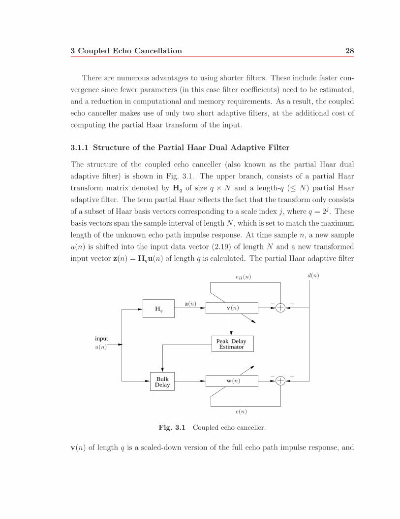
3.1.1 Structure of the Partial Haar Dual Adaptive Filter
The structure of the coupled echo canceller (also known as the partial Haar dual
adaptive filter) is shown in Fig. 3.1. The upper branch, consists of a partial Haar
transform matrix denoted by Hq of size q × N and a length-q (≤ N) partial Haar
adaptive filter. The term partial Haar reflects the fact that the transform only consists
of a subset of Haar basis vectors corresponding to a scale index j, where q = 2j. These
basis vectors span the sample interval of length N , which is set to match the maximum
length of the unknown echo path impulse response. At time sample n, a new sample
u(n) is shifted into the input data vector (2.19) of length N and a new transformed
input vector z(n) = Hqu(n) of length q is calculated. The partial Haar adaptive filter
input
DelayBulk
Peak DelayEstimator
Hq
u(n)
z(n)
−
−
+
+
eH(n)
e(n)
d(n)
v(n)
w(n)
Fig. 3.1 Coupled echo canceller.
v(n) of length q is a scaled-down version of the full echo path impulse response, and
3 Coupled Echo Cancellation 29
is used solely to track changes in the echo path impulse response. The peak delay
estimator tracks the location of the dispersive region by locating the peak magnitude
of the partial Haar impulse response.
In the lower branch of the echo canceller, the estimated location of the dispersive
region is used to offset (using an appropriate bulk delay) a short time-domain filter
w(n) of length L so that it is properly centred around the dispersive region. The
length of the time-domain filter is set to match the longest expected dispersive region
in the echo path.
3.1.2 Effect of the Complete Haar Transform on the Wiener Solution
This subsection deals with the effect of the complete Haar transform on the Wiener
solution. Let HN denote the orthogonal N×N Haar transform matrix, i.e. HTNHN =
HNHTN = IN , and z(n) = HNu(n) is the transformed input vector of length N . The
optimal Haar weight vector is denoted by vo (in this case, the length of vo is N). The
resulting Wiener-Hopf equation is given by
Rzzvo = pz, (3.1)
where Rzz = E[z(n)zT (n)] = HNRuuHTN represents the autocorrelation matrix of
z(n), and pz = E[z(n)d(n)] = HNpu is the cross-correlation vector between z(n) and
the desired signal d(n). Solving for vo,
vo = R−1zz pz
= {HNRuuHTN}−1HNpu
= HNR−1uuHT
NHNpu
= HN
[R−1
uupu
]= HNwo. (3.2)
As a consequence of the orthogonality property of the Haar transform matrix, the
Wiener solution corresponding to the transformed input data vector is simply the
Haar transform of the time-domain Wiener solution. In fact, it is possible to recover
the optimal time-domain Wiener solution by pre-multiplying (3.2) by HTN .

3 Coupled Echo Cancellation 30
3.1.3 Effect of the Partial Haar Transform on the Wiener Solution
It was seen in the previous section that by transforming the input with the set of
Haar basis vectors, the Wiener solution is also transformed. When only a subset of
Haar basis vectors at a scale index j is used to transform the input, the situation is
somewhat different. Unlike the complete Haar transform matrix, Hq (q < N) is only
row-wise orthogonal, i.e. HqHTq = Iq �= HT
q Hq.
The terms Rzz and pz have the same interpretation as in the previous section,
except all quantities are now based on the partially transformed input z(n) = Hqu(n)
(q < N). The resulting Wiener-Hopf equation becomes
vo = R−1zz pz
= {E[z(n)zT (n)]}−1E[z(n)d(n)]
= {E[Hqu(n)uT (n)HTq ]}−1E[Hqu(n)d(n)]
= {HqRuuHTq }−1Hqpu. (3.3)
The above equation cannot be simplified any further, mainly because the partial
Haar transform matrix is only row-wise orthogonal. If one assumes, however, that the
input is white with Ruu = σ2uIN , then
vo = {Hqσ2uH
Tq }−1Hqpu
= Hqpu/σ2u
= Hqwo. (3.4)
The result is similar to the complete Haar transform, provided the input samples are
uncorrelated. However, it is not possible to recover the original Wiener solution. In
addition, it is interesting to observe that no transformation of the desired signal d(n)
is necessary.
Now that the effect of the partial Haar transform on the Wiener solution has been
investigated, consider its effect on the minimum mean square error Jmin, which is
calculated by taking the expected value of the minimum squared error, eHo(n), of the
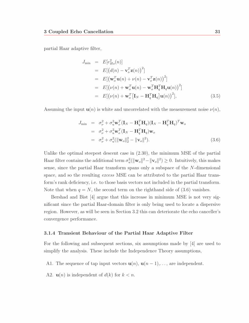
3 Coupled Echo Cancellation 31
partial Haar adaptive filter,
Jmin = E[e2Ho(n)]
= E[(d(n) − vT
o z(n))2
]
= E[(wT
o u(n) + ν(n) − vTo z(n)
)2]
= E[(ν(n) + wT
o u(n) − wTo HT
q Hqu(n))2
]
= E[(ν(n) + wT
o
[IN − HT
q Hq
]u(n)
)2], (3.5)
Assuming the input u(n) is white and uncorrelated with the measurement noise ν(n),
Jmin = σ2ν + σ2
uwTo (IN − HT
q Hq)(IN − HTq Hq)
Two
= σ2ν + σ2
uwTo (IN − HT
q Hq)wo
= σ2ν + σ2
u(‖wo‖22 − ‖vo‖2). (3.6)
Unlike the optimal steepest descent case in (2.30), the minimum MSE of the partial
Haar filter contains the additional term σ2u(‖wo‖2−‖vo‖2) ≥ 0. Intuitively, this makes
sense, since the partial Haar transform spans only a subspace of the N -dimensional
space, and so the resulting excess MSE can be attributed to the partial Haar trans-
form’s rank deficiency, i.e. to those basis vectors not included in the partial transform.
Note that when q = N , the second term on the righthand side of (3.6) vanishes.
Bershad and Bist [4] argue that this increase in minimum MSE is not very sig-
nificant since the partial Haar-domain filter is only being used to locate a dispersive
region. However, as will be seen in Section 3.2 this can deteriorate the echo canceller’s
convergence performance.
3.1.4 Transient Behaviour of the Partial Haar Adaptive Filter
For the following and subsequent sections, six assumptions made by [4] are used to
simplify the analysis. These include the Independence Theory assumptions,
A1. The sequence of tap input vectors u(n), u(n− 1),. . . , are independent.
A2. u(n) is independent of d(k) for k < n.

3 Coupled Echo Cancellation 32
A3. d(n) depends on u(n) but not on d(k), for k < n.
Additional assumptions are used to simplify the analysis,
A4. The sequences of input samples u(k) and desired responses d(m) are zero-mean
jointly Gaussian.
A5. u(n) is stationary and white, i.e. E[u(n)uT (n)] = σ2uIN .
Finally, to make the analyze of the peak delay estimator easier, it is assumed that
A6. The partial Haar weight vector, v(n), is a jointly Gaussian random vector.
The partial Haar LMS weight recursion formula adapted from (2.34) is given by
v(n+ 1) = v(n) + μeH(n)z(n) (3.7)
where
eH(n) = d(n) − zT (n)v(n). (3.8)
Replacing (3.8) into (3.7) yields
v(n+ 1) = [Iq − μz(n)zT (n)]v(n) + μd(n)z(n), (3.9)
Taking the expectation of both sides of (3.9), and using A1 and A5 along with (3.3),
E[v(n+ 1)] = [1 − μσ2u]E[v(n)] + μσ2
uvo. (3.10)
The closed-form expression for the solution of the above equation is
E[v(n)] = (1 − μσ2u)
nv(0) + [1 − (1 − μσ2u)
n]vo. (3.11)
Therefore as n increases and provided that 0 < μ < 2/σ2u, the expected weight vector
approaches the optimal partial Haar weight vector vo.
3 Coupled Echo Cancellation 33
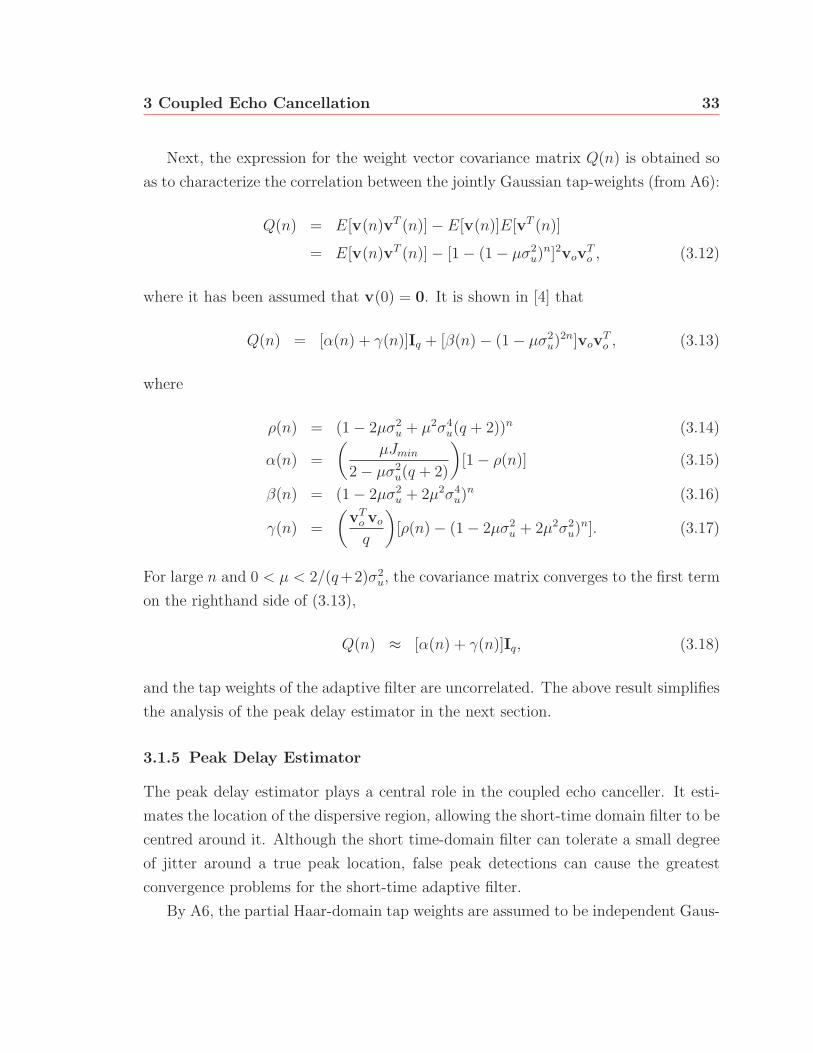
Next, the expression for the weight vector covariance matrix Q(n) is obtained so
as to characterize the correlation between the jointly Gaussian tap-weights (from A6):
Q(n) = E[v(n)vT (n)] − E[v(n)]E[vT (n)]
= E[v(n)vT (n)] − [1 − (1 − μσ2u)
n]2vovTo , (3.12)
where it has been assumed that v(0) = 0. It is shown in [4] that
Q(n) = [α(n) + γ(n)]Iq + [β(n) − (1 − μσ2u)
2n]vovTo , (3.13)
where
ρ(n) = (1 − 2μσ2u + μ2σ4
u(q + 2))n (3.14)
α(n) =
(μJmin
2 − μσ2u(q + 2)
)[1 − ρ(n)] (3.15)
β(n) = (1 − 2μσ2u + 2μ2σ4
u)n (3.16)
γ(n) =
(vT
o vo
q
)[ρ(n) − (1 − 2μσ2
u + 2μ2σ2u)
n]. (3.17)
For large n and 0 < μ < 2/(q+2)σ2u, the covariance matrix converges to the first term
on the righthand side of (3.13),
Q(n) ≈ [α(n) + γ(n)]Iq, (3.18)
and the tap weights of the adaptive filter are uncorrelated. The above result simplifies
the analysis of the peak delay estimator in the next section.
3.1.5 Peak Delay Estimator
The peak delay estimator plays a central role in the coupled echo canceller. It esti-
mates the location of the dispersive region, allowing the short-time domain filter to be
centred around it. Although the short time-domain filter can tolerate a small degree
of jitter around a true peak location, false peak detections can cause the greatest
convergence problems for the short-time adaptive filter.
By A6, the partial Haar-domain tap weights are assumed to be independent Gaus-
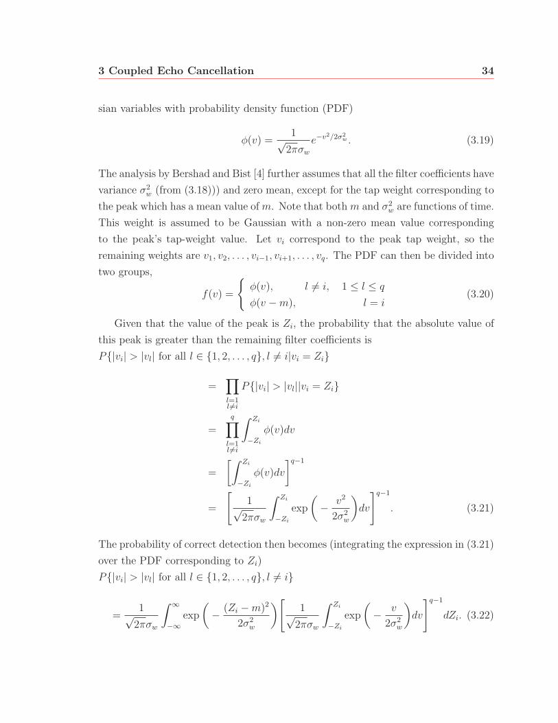
3 Coupled Echo Cancellation 34
sian variables with probability density function (PDF)
φ(v) =1√
2πσw
e−v2/2σ2w . (3.19)
The analysis by Bershad and Bist [4] further assumes that all the filter coefficients have
variance σ2w (from (3.18))) and zero mean, except for the tap weight corresponding to
the peak which has a mean value of m. Note that both m and σ2w are functions of time.
This weight is assumed to be Gaussian with a non-zero mean value corresponding
to the peak’s tap-weight value. Let vi correspond to the peak tap weight, so the
remaining weights are v1, v2, . . . , vi−1, vi+1, . . . , vq. The PDF can then be divided into
two groups,
f(v) =
{φ(v), l �= i, 1 ≤ l ≤ q
φ(v −m), l = i(3.20)
Given that the value of the peak is Zi, the probability that the absolute value of
this peak is greater than the remaining filter coefficients is
P{|vi| > |vl| for all l ∈ {1, 2, . . . , q}, l �= i|vi = Zi}
=∏l=1l �=i
P{|vi| > |vl||vi = Zi}
=
q∏l=1l �=i
∫ Zi
−Zi
φ(v)dv
=
[∫ Zi
−Zi
φ(v)dv
]q−1
=
[1√
2πσw
∫ Zi
−Zi
exp
(− v2
2σ2w
)dv
]q−1
. (3.21)
The probability of correct detection then becomes (integrating the expression in (3.21)
over the PDF corresponding to Zi)
P{|vi| > |vl| for all l ∈ {1, 2, . . . , q}, l �= i}
=1√
2πσw
∫ ∞
−∞exp
(− (Zi −m)2
2σ2w
)[1√
2πσw
∫ Zi
−Zi
exp
(− v
2σ2w
)dv
]q−1
dZi. (3.22)
3 Coupled Echo Cancellation 35
3.2 Critical Analysis of the Haar-domain Adaptive Filter
This section provides an in depth look at the significant drawbacks of the coupled
echo canceller [4]. These include its dependence on the echo path’s bulk delay, the
problem of tracking dispersive regions in non-stationary environments, and the lack
of provision for locating multiple dispersive regions.
3.2.1 Effect of the Bulk Delay on the Partial Haar Impulse Response
In Section 3.1.3 the effect of transforming a white input signal (prior to filtering)
with the partial Haar transform on the optimal Wiener solution was studied. It was
shown that the resulting Wiener solution is simply the partial Haar transform of the
time-domain Wiener solution. Recall from Section 2.1, however, that one of the main
disadvantages of wavelet transforms is their lack of shift invariance. In other words,
depending on the bulk delay of the dispersive region, the transformed Wiener solution
can be quite different, changing the peak delay estimator’s performance.
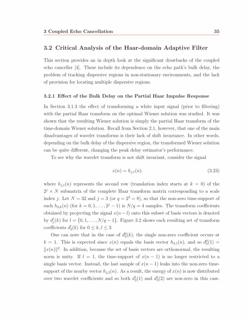
To see why the wavelet transform is not shift invariant, consider the signal
x(n) = hj,1(n). (3.23)
where hj,1(n) represents the second row (translation index starts at k = 0) of the
2j × N submatrix of the complete Haar transform matrix corresponding to a scale
index j. Let N = 32 and j = 3 (or q = 23 = 8), so that the non-zero time-support of
each h3,k(n) (for k = 0, 1, . . . , 2j − 1) is N/q = 4 samples. The transform coefficients
obtained by projecting the signal x(n− l) onto this subset of basis vectors is denoted
by dlj(k) for l = {0, 1, . . . , N/q − 1}. Figure 3.2 shows each resulting set of transform
coefficients dl3(k) for 0 ≤ k, l ≤ 3.
One can note that in the case of d03(k), the single non-zero coefficient occurs at
k = 1. This is expected since x(n) equals the basis vector h3,1(n), and so d03(1) =
‖x(n)‖2. In addition, because the set of basis vectors are orthonormal, the resulting
norm is unity. If l = 1, the time-support of x(n − 1) is no longer restricted to a
single basis vector. Instead, the last sample of x(n− 1) leaks into the non-zero time-
support of the nearby vector hj,2(n). As a result, the energy of x(n) is now distributed
over two wavelet coefficients and so both d13(1) and d1
3(2) are non-zero in this case.
3 Coupled Echo Cancellation 36
Furthermore, by Parseval’s relation (2.14), |d13(1)|2, |d1
3(2)|2 < 1. In other words, the
peak magnitude for this case is smaller than for d03(k).
As l increases, the energy of x(n − l) is distributed across both the second and
third wavelet basis vectors, h3,1 and h3,2. When l = 4, x(n − 4) = hj,2(n), the
subsequent observations for l = {4, 5, 6, 7} are identical to the case for l = {1, 2, 3, 4}in Fig. 3.2. In other words, although the DWT is not strictly shift invariant [8, 43],
it is periodically invariant with a period of N/q.
0
0
0.5
−0.5
1
1 2 3
d0 j(k
)
k
(a)
0
0
0.5
−0.5
1
1 2 3d1 j(k
)
k
(b)
0
0
0.5
−0.5
1
1 2 3
d2 j(k
)
k
(c)
0
0
0.5
−0.5
1
1 2 3
d3 j(k
)
k
(d)
Fig. 3.2 Examining the lack of shift invariance of the wavelet transformfor N = 32, q = 8, corresponding to (a) l = 0 (b) 1 (c) 2 (d) 3 sample(s).
From the above observations, one can conclude that for a given echo path impulse
response, the partial Haar Wiener solution depends on the bulk delay. In addition, it
turns out that for q = 2j, there actually exist N/q unique partial Haar transformed
impulse responses. Furthermore, the respective peak magnitudes of each of these
transformed impulse responses can be different, and consequently the amount of time

3 Coupled Echo Cancellation 37
it takes the peak delay estimator to correctly estimate the location of a dispersive
region varies. This can significantly affect the overall convergence speed of the cou-
pled echo canceller. For example, consider the set of N/q = 1024/256 partial Haar
transforms of an echo path impulse response containing an ITU-T G.168 hybrid im-
pulse response m5(n) in Fig. 3.3. One can clearly observe that the third case displays
50
50
50
50
150
150
150
150
200
200
200
200
250
250
250
250
100
100
100
100
00
00
00
00
0.05
0.05
0.05
0.05
0.1
0.1
0.1
0.1
samples
Fig. 3.3 Set of transformed impulse responses corresponding to m5(n).
a diminished peak. In addition, as a result of measurement noise and the effect of
the partial Haar transform on the minimum MSE in (3.6), the peak delay estimator
takes a longer time to locate small peaks. To support this claim, consider the family
of CDF curves in Fig. 3.4 corresponding to the time to correctly locate the dispersive
region for four different bulk delays (each curve is identified by its peak magnitude).
It is apparent from this figure that it takes the peak delay estimator a larger number
of input samples to correctly locate a smaller peak. For example, for the curve corre-
sponding to a peak magnitude of 0.0166, the peak delay estimator can barely locate
the peak after 103 input samples. An algorithm will be proposed in the next chapter
to escape such suboptimal cases.
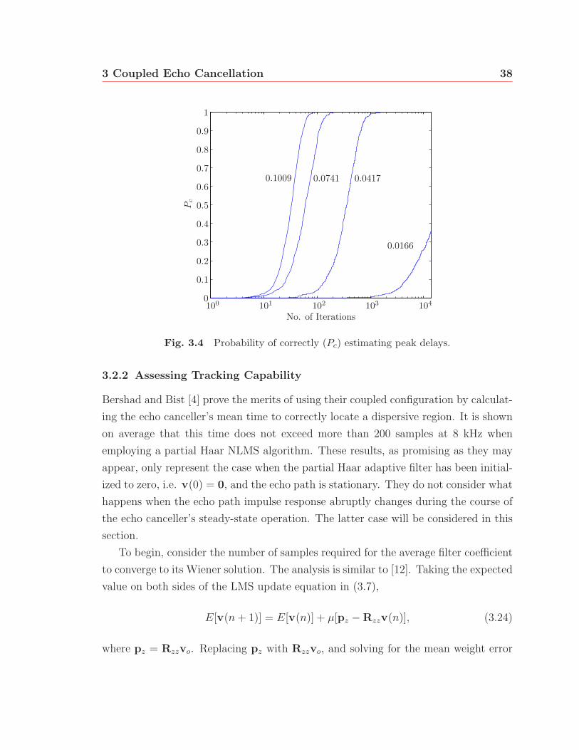
3 Coupled Echo Cancellation 38
100 101 102 103 104
0.0417
0.0166
0.1009 0.0741
0
0.1
0.2
0.3
0.4
0.5
0.6
0.7
0.8
0.9
1
No. of Iterations
Pc
Fig. 3.4 Probability of correctly (Pc) estimating peak delays.
3.2.2 Assessing Tracking Capability
Bershad and Bist [4] prove the merits of using their coupled configuration by calculat-
ing the echo canceller’s mean time to correctly locate a dispersive region. It is shown
on average that this time does not exceed more than 200 samples at 8 kHz when
employing a partial Haar NLMS algorithm. These results, as promising as they may
appear, only represent the case when the partial Haar adaptive filter has been initial-
ized to zero, i.e. v(0) = 0, and the echo path is stationary. They do not consider what
happens when the echo path impulse response abruptly changes during the course of
the echo canceller’s steady-state operation. The latter case will be considered in this
section.
To begin, consider the number of samples required for the average filter coefficient
to converge to its Wiener solution. The analysis is similar to [12]. Taking the expected
value on both sides of the LMS update equation in (3.7),
E[v(n+ 1)] = E[v(n)] + μ[pz − Rzzv(n)], (3.24)
where pz = Rzzvo. Replacing pz with Rzzvo, and solving for the mean weight error
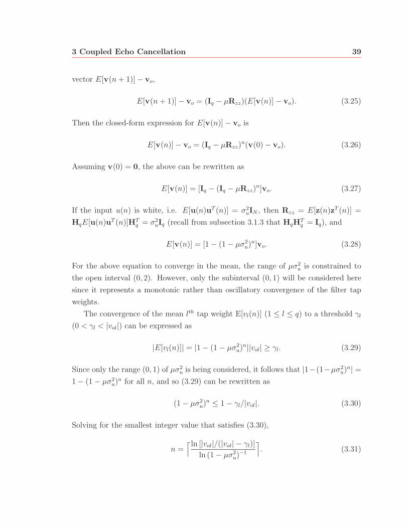
3 Coupled Echo Cancellation 39
vector E[v(n+ 1)] − vo,
E[v(n+ 1)] − vo = (Iq − μRzz)(E[v(n)] − vo). (3.25)
Then the closed-form expression for E[v(n)] − vo is
E[v(n)] − vo = (Iq − μRzz)n(v(0) − vo). (3.26)
Assuming v(0) = 0, the above can be rewritten as
E[v(n)] = [Iq − (Iq − μRzz)n]vo. (3.27)
If the input u(n) is white, i.e. E[u(n)uT (n)] = σ2uIN , then Rzz = E[z(n)zT (n)] =
HqE[u(n)uT (n)]HTq = σ2
uIq (recall from subsection 3.1.3 that HqHTq = Iq), and
E[v(n)] = [1 − (1 − μσ2u)
n]vo. (3.28)
For the above equation to converge in the mean, the range of μσ2u is constrained to
the open interval (0, 2). However, only the subinterval (0, 1) will be considered here
since it represents a monotonic rather than oscillatory convergence of the filter tap
weights.
The convergence of the mean lth tap weight E[vl(n)] (1 ≤ l ≤ q) to a threshold γl
(0 < γl < |vol|) can be expressed as
|E[vl(n)]| = |1 − (1 − μσ2u)
n||vol| ≥ γl. (3.29)
Since only the range (0, 1) of μσ2u is being considered, it follows that |1−(1−μσ2
u)n| =
1 − (1 − μσ2u)
n for all n, and so (3.29) can be rewritten as
(1 − μσ2u)
n ≤ 1 − γl/|vol|. (3.30)
Solving for the smallest integer value that satisfies (3.30),
n =⌈ ln [|vol|/(|vol| − γl)]
ln (1 − μσ2u)
−1
⌉. (3.31)
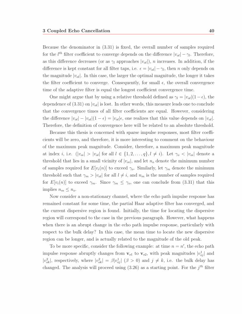
3 Coupled Echo Cancellation 40
Because the denominator in (3.31) is fixed, the overall number of samples required
for the lth filter coefficient to converge depends on the difference |vol| − γl. Therefore,
as this difference decreases (or as γl approaches |vol|), n increases. In addition, if the
difference is kept constant for all filter taps, i.e. ε = |vol|− γl, then n only depends on
the magnitude |vol|. In this case, the larger the optimal magnitude, the longer it takes
the filter coefficient to converge. Consequently, for small ε, the overall convergence
time of the adaptive filter is equal the longest coefficient convergence time.
One might argue that by using a relative threshold defined as γl = |vol|(1− ε), the
dependence of (3.31) on |vol| is lost. In other words, this measure leads one to conclude
that the convergence times of all filter coefficients are equal. However, considering
the difference |vol| − |vol|(1 − ε) = |vol|ε, one realizes that this value depends on |vol|.Therefore, the definition of convergence here will be related to an absolute threshold.
Because this thesis is concerned with sparse impulse responses, most filter coeffi-
cients will be zero, and therefore, it is more interesting to comment on the behaviour
of the maximum peak magnitude. Consider, therefore, a maximum peak magnitude
at index i, i.e. (|voi| > |vol| for all l ∈ {1, 2, . . . , q}, l �= i). Let γo < |voi| denote a
threshold that lies in a small vicinity of |voi|, and let no denote the minimum number
of samples required for E[vi(n)] to exceed γo. Similarly, let γm denote the minimum
threshold such that γm > |vol| for all l �= i, and nm is the number of samples required
for E[vi(n)] to exceed γm. Since γm ≤ γo, one can conclude from (3.31) that this
implies nm ≤ no.
Now consider a non-stationary channel, where the echo path impulse response has
remained constant for some time, the partial Haar adaptive filter has converged, and
the current dispersive region is found. Initially, the time for locating the dispersive
region will correspond to the case in the previous paragraph. However, what happens
when there is an abrupt change in the echo path impulse response, particularly with
respect to the bulk delay? In this case, the mean time to locate the new dispersive
region can be longer, and is actually related to the magnitude of the old peak.
To be more specific, consider the following example: at time n = n′, the echo path
impulse response abruptly changes from vo1 to vo2, with peak magnitudes |v1oj| and
|v2ok|, respectively, where |v2
ok| = β|v1oj| (β > 0) and j �= k, i.e. the bulk delay has
changed. The analysis will proceed using (3.26) as a starting point. For the jth filter
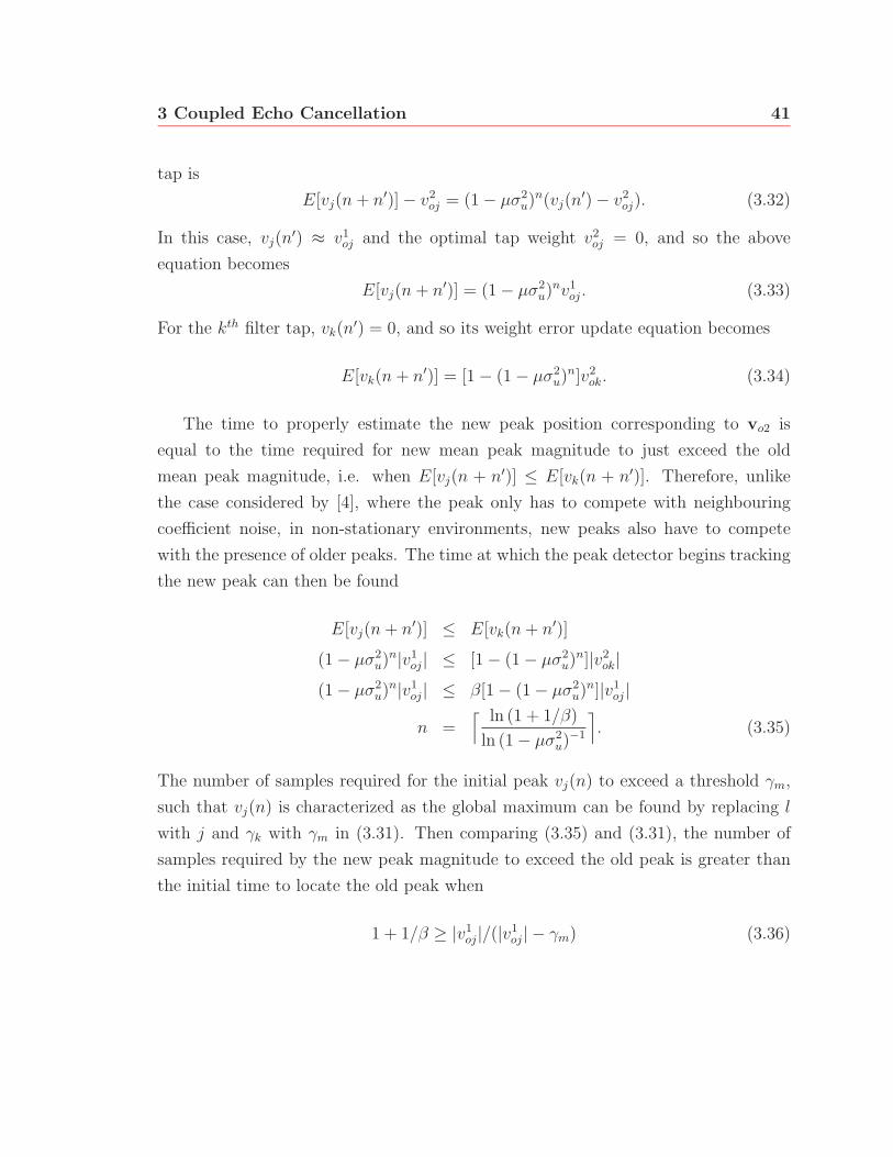
3 Coupled Echo Cancellation 41
tap is
E[vj(n+ n′)] − v2oj = (1 − μσ2
u)n(vj(n
′) − v2oj). (3.32)
In this case, vj(n′) ≈ v1
oj and the optimal tap weight v2oj = 0, and so the above
equation becomes
E[vj(n+ n′)] = (1 − μσ2u)
nv1oj. (3.33)
For the kth filter tap, vk(n′) = 0, and so its weight error update equation becomes
E[vk(n+ n′)] = [1 − (1 − μσ2u)
n]v2ok. (3.34)
The time to properly estimate the new peak position corresponding to vo2 is
equal to the time required for new mean peak magnitude to just exceed the old
mean peak magnitude, i.e. when E[vj(n + n′)] ≤ E[vk(n + n′)]. Therefore, unlike
the case considered by [4], where the peak only has to compete with neighbouring
coefficient noise, in non-stationary environments, new peaks also have to compete
with the presence of older peaks. The time at which the peak detector begins tracking
the new peak can then be found
E[vj(n+ n′)] ≤ E[vk(n+ n′)]
(1 − μσ2u)
n|v1oj| ≤ [1 − (1 − μσ2
u)n]|v2
ok|(1 − μσ2
u)n|v1
oj| ≤ β[1 − (1 − μσ2u)
n]|v1oj|
n =⌈ ln (1 + 1/β)
ln (1 − μσ2u)
−1
⌉. (3.35)
The number of samples required for the initial peak vj(n) to exceed a threshold γm,
such that vj(n) is characterized as the global maximum can be found by replacing l
with j and γk with γm in (3.31). Then comparing (3.35) and (3.31), the number of
samples required by the new peak magnitude to exceed the old peak is greater than
the initial time to locate the old peak when
1 + 1/β ≥ |v1oj|/(|v1
oj| − γm) (3.36)
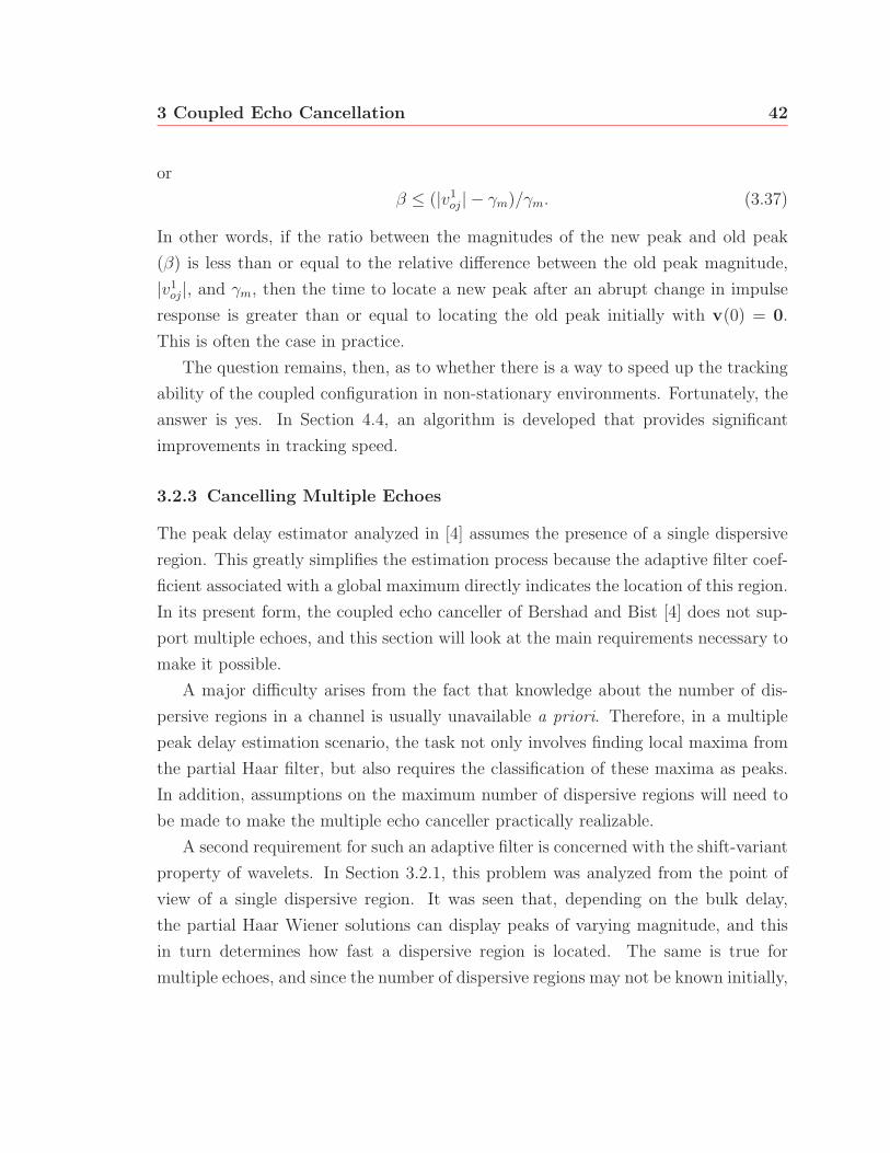
3 Coupled Echo Cancellation 42
or
β ≤ (|v1oj| − γm)/γm. (3.37)
In other words, if the ratio between the magnitudes of the new peak and old peak
(β) is less than or equal to the relative difference between the old peak magnitude,
|v1oj|, and γm, then the time to locate a new peak after an abrupt change in impulse
response is greater than or equal to locating the old peak initially with v(0) = 0.
This is often the case in practice.
The question remains, then, as to whether there is a way to speed up the tracking
ability of the coupled configuration in non-stationary environments. Fortunately, the
answer is yes. In Section 4.4, an algorithm is developed that provides significant
improvements in tracking speed.
3.2.3 Cancelling Multiple Echoes
The peak delay estimator analyzed in [4] assumes the presence of a single dispersive
region. This greatly simplifies the estimation process because the adaptive filter coef-
ficient associated with a global maximum directly indicates the location of this region.
In its present form, the coupled echo canceller of Bershad and Bist [4] does not sup-
port multiple echoes, and this section will look at the main requirements necessary to
make it possible.
A major difficulty arises from the fact that knowledge about the number of dis-
persive regions in a channel is usually unavailable a priori. Therefore, in a multiple
peak delay estimation scenario, the task not only involves finding local maxima from
the partial Haar filter, but also requires the classification of these maxima as peaks.
In addition, assumptions on the maximum number of dispersive regions will need to
be made to make the multiple echo canceller practically realizable.
A second requirement for such an adaptive filter is concerned with the shift-variant
property of wavelets. In Section 3.2.1, this problem was analyzed from the point of
view of a single dispersive region. It was seen that, depending on the bulk delay,
the partial Haar Wiener solutions can display peaks of varying magnitude, and this
in turn determines how fast a dispersive region is located. The same is true for
multiple echoes, and since the number of dispersive regions may not be known initially,
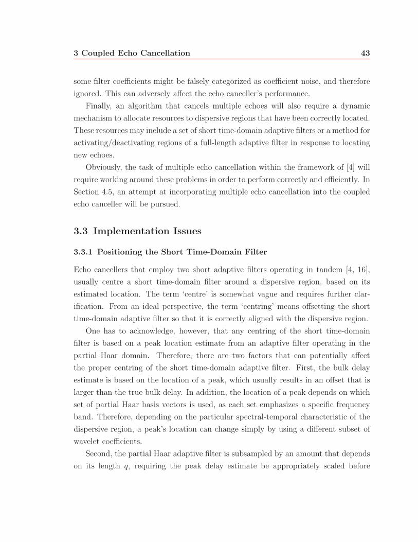
3 Coupled Echo Cancellation 43
some filter coefficients might be falsely categorized as coefficient noise, and therefore
ignored. This can adversely affect the echo canceller’s performance.
Finally, an algorithm that cancels multiple echoes will also require a dynamic
mechanism to allocate resources to dispersive regions that have been correctly located.
These resources may include a set of short time-domain adaptive filters or a method for
activating/deactivating regions of a full-length adaptive filter in response to locating
new echoes.
Obviously, the task of multiple echo cancellation within the framework of [4] will
require working around these problems in order to perform correctly and efficiently. In
Section 4.5, an attempt at incorporating multiple echo cancellation into the coupled
echo canceller will be pursued.
3.3 Implementation Issues
3.3.1 Positioning the Short Time-Domain Filter
Echo cancellers that employ two short adaptive filters operating in tandem [4, 16],
usually centre a short time-domain filter around a dispersive region, based on its
estimated location. The term ‘centre’ is somewhat vague and requires further clar-
ification. From an ideal perspective, the term ‘centring’ means offsetting the short
time-domain adaptive filter so that it is correctly aligned with the dispersive region.
One has to acknowledge, however, that any centring of the short time-domain
filter is based on a peak location estimate from an adaptive filter operating in the
partial Haar domain. Therefore, there are two factors that can potentially affect
the proper centring of the short time-domain adaptive filter. First, the bulk delay
estimate is based on the location of a peak, which usually results in an offset that is
larger than the true bulk delay. In addition, the location of a peak depends on which
set of partial Haar basis vectors is used, as each set emphasizes a specific frequency
band. Therefore, depending on the particular spectral-temporal characteristic of the
dispersive region, a peak’s location can change simply by using a different subset of
wavelet coefficients.
Second, the partial Haar adaptive filter is subsampled by an amount that depends
on its length q, requiring the peak delay estimate be appropriately scaled before
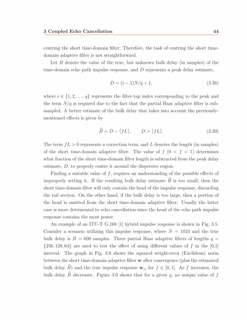
3 Coupled Echo Cancellation 44
centring the short time-domain filter. Therefore, the task of centring the short time-
domain adaptive filter is not straightforward.
Let B denote the value of the true, but unknown bulk delay (in samples) of the
time-domain echo path impulse response, and D represents a peak delay estimate,
D = (i− 1)N/q + 1, (3.38)
where i ∈ {1, 2, . . . , q} represents the filter-tap index corresponding to the peak and
the term N/q is required due to the fact that the partial Haar adaptive filter is sub-
sampled. A better estimate of the bulk delay that takes into account the previously-
mentioned effects is given by
B = D − �fL�, D > �fL�. (3.39)
The term fL > 0 represents a correction term, and L denotes the length (in samples)
of the short time-domain adaptive filter. The value of f (0 < f < 1) determines
what fraction of the short time-domain filter length is subtracted from the peak delay
estimate, D, to properly centre it around the dispersive region.
Finding a suitable value of f , requires an understanding of the possible effects of
improperly setting it. If the resulting bulk delay estimate B is too small, then the
short time-domain filter will only contain the head of the impulse response, discarding
the tail section. On the other hand, if the bulk delay is too large, then a portion of
the head is omitted from the short time-domain adaptive filter. Usually the latter
case is more detrimental to echo cancellation since the head of the echo path impulse
response contains the most power.
An example of an ITU-T G.168 [1] hybrid impulse response is shown in Fig. 3.5.
Consider a scenario utilizing this impulse response, where N = 1024 and the true
bulk delay is B = 600 samples. Three partial Haar adaptive filters of lengths q =
{256, 128, 64} are used to test the effect of using different values of f in the [0,1]
interval. The graph in Fig. 3.6 shows the squared weight-error (Euclidean) norm
between the short time-domain adaptive filter w after convergence (plus the estimated
bulk delay B) and the true impulse response wo, for f ∈ [0, 1]. As f increases, the
bulk delay B decreases. Figure 3.6 shows that for a given q, no unique value of f
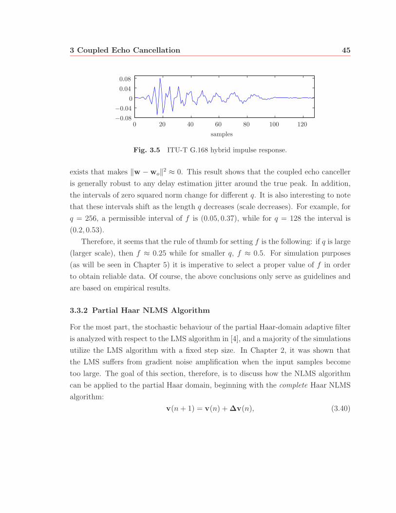
3 Coupled Echo Cancellation 45
0
0
0.040.08
−0.04−0.08
20 40 60 80 100 120samples
Fig. 3.5 ITU-T G.168 hybrid impulse response.
exists that makes ‖w − wo‖2 ≈ 0. This result shows that the coupled echo canceller
is generally robust to any delay estimation jitter around the true peak. In addition,
the intervals of zero squared norm change for different q. It is also interesting to note
that these intervals shift as the length q decreases (scale decreases). For example, for
q = 256, a permissible interval of f is (0.05, 0.37), while for q = 128 the interval is
(0.2, 0.53).
Therefore, it seems that the rule of thumb for setting f is the following: if q is large
(larger scale), then f ≈ 0.25 while for smaller q, f ≈ 0.5. For simulation purposes
(as will be seen in Chapter 5) it is imperative to select a proper value of f in order
to obtain reliable data. Of course, the above conclusions only serve as guidelines and
are based on empirical results.
3.3.2 Partial Haar NLMS Algorithm
For the most part, the stochastic behaviour of the partial Haar-domain adaptive filter
is analyzed with respect to the LMS algorithm in [4], and a majority of the simulations
utilize the LMS algorithm with a fixed step size. In Chapter 2, it was shown that
the LMS suffers from gradient noise amplification when the input samples become
too large. The goal of this section, therefore, is to discuss how the NLMS algorithm
can be applied to the partial Haar domain, beginning with the complete Haar NLMS
algorithm:
v(n+ 1) = v(n) + Δv(n), (3.40)

3 Coupled Echo Cancellation 46
00
0.005
0.01
0.015
0.02
0.025
0.03
0.035
0.04
0.045
0.1 0.2 0.3 0.4 0.5 0.6 0.7 0.8 0.9 1f
‖w−
wo‖2
q = 256q = 128q = 64
Fig. 3.6 The mean-squared weight error plotted for three different par-tial Haar adaptive filter lengths q = 256, 128, 64.
with
Δv(n) =μ
‖z(n)‖2z(n)eH(n) (3.41)
eH(n) = d(n) − zT (n)v(n), (3.42)
where z(n) = HNu(n) is the transformed input vector and v(n) is the weight vec-
tor. Because HN is an orthogonal matrix (HTNHN = HNHT
N = IN), it follows that
‖z(n)‖2 = zT (n)z(n) = uT (n)HTNHNu(n) = ‖u(n)‖2. In addition, the convergence
behaviour of both filters is the same, since the eigenvalues of the transformed input
correlation matrix are equal to the eigenvalues of the original autocorrelation matrix.
This can be shown by observing the characteristic equation,
0 = det[λI − Rzz]
= det[HN(λI − Ruu)HTN ]
= det[λI − Ruu]. (3.43)
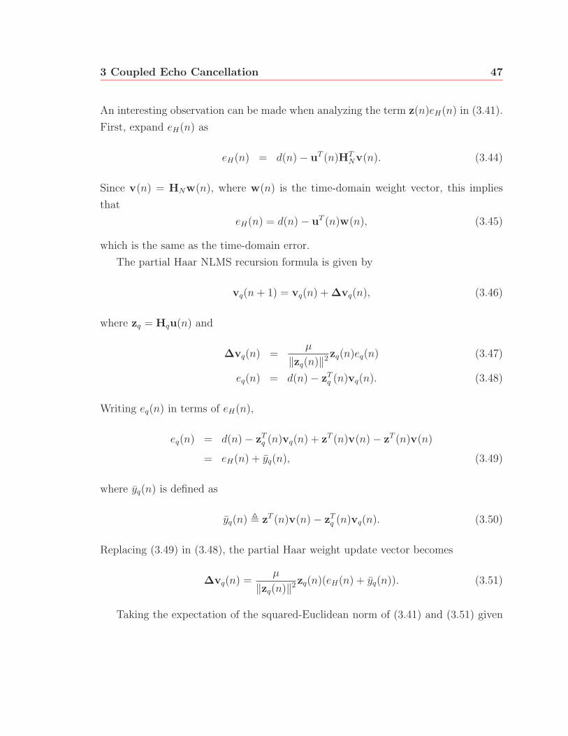
3 Coupled Echo Cancellation 47
An interesting observation can be made when analyzing the term z(n)eH(n) in (3.41).
First, expand eH(n) as
eH(n) = d(n) − uT (n)HTNv(n). (3.44)
Since v(n) = HNw(n), where w(n) is the time-domain weight vector, this implies
that
eH(n) = d(n) − uT (n)w(n), (3.45)
which is the same as the time-domain error.
The partial Haar NLMS recursion formula is given by
vq(n+ 1) = vq(n) + Δvq(n), (3.46)
where zq = Hqu(n) and
Δvq(n) =μ
‖zq(n)‖2zq(n)eq(n) (3.47)
eq(n) = d(n) − zTq (n)vq(n). (3.48)
Writing eq(n) in terms of eH(n),
eq(n) = d(n) − zTq (n)vq(n) + zT (n)v(n) − zT (n)v(n)
= eH(n) + yq(n), (3.49)
where yq(n) is defined as
yq(n) � zT (n)v(n) − zTq (n)vq(n). (3.50)
Replacing (3.49) in (3.48), the partial Haar weight update vector becomes
Δvq(n) =μ
‖zq(n)‖2zq(n)(eH(n) + yq(n)). (3.51)
Taking the expectation of the squared-Euclidean norm of (3.41) and (3.51) given
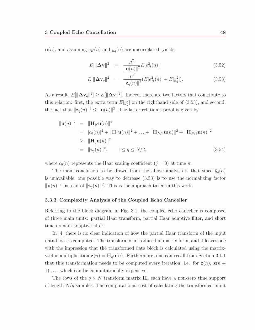
3 Coupled Echo Cancellation 48
u(n), and assuming eH(n) and yq(n) are uncorrelated, yields
E[‖Δv‖2] =μ2
‖u(n)‖2E[e2H(n)] (3.52)
E[‖Δvq‖2] =μ2
‖zq(n)‖2 (E[e2H(n)] + E[y2
q ]). (3.53)
As a result, E[‖Δvq‖2] ≥ E[‖Δv‖2]. Indeed, there are two factors that contribute to
this relation: first, the extra term E[y2q ] on the righthand side of (3.53), and second,
the fact that ‖zq(n)‖2 ≤ ‖u(n)‖2. The latter relation’s proof is given by
‖u(n)‖2 = ‖HNu(n)‖2
= |c0(n)|2 + ‖H1u(n)‖2 + . . .+ ‖HN/4u(n)‖2 + ‖HN/2u(n)‖2
≥ ‖Hqu(n)‖2
= ‖zq(n)‖2, 1 ≤ q ≤ N/2, (3.54)
where c0(n) represents the Haar scaling coefficient (j = 0) at time n.
The main conclusion to be drawn from the above analysis is that since yq(n)
is unavailable, one possible way to decrease (3.53) is to use the normalizing factor
‖u(n)‖2 instead of ‖zq(n)‖2. This is the approach taken in this work.
3.3.3 Complexity Analysis of the Coupled Echo Canceller
Referring to the block diagram in Fig. 3.1, the coupled echo canceller is composed
of three main units: partial Haar transform, partial Haar adaptive filter, and short
time-domain adaptive filter.
In [4] there is no clear indication of how the partial Haar transform of the input
data block is computed. The transform is introduced in matrix form, and it leaves one
with the impression that the transformed data block is calculated using the matrix-
vector multiplication z(n) = Hqu(n). Furthermore, one can recall from Section 3.1.1
that this transformation needs to be computed every iteration, i.e. for z(n), z(n +
1),. . . , which can be computationally expensive.
The rows of the q × N transform matrix Hq each have a non-zero time support
of length N/q samples. The computational cost of calculating the transformed input
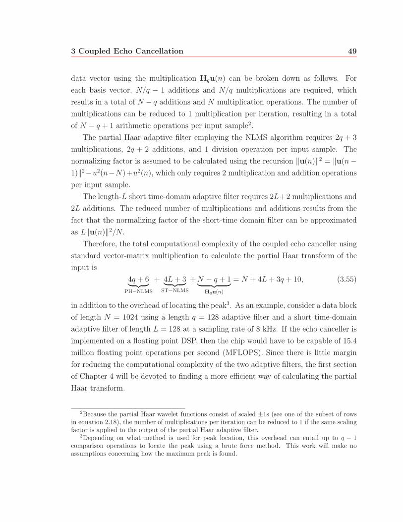
3 Coupled Echo Cancellation 49
data vector using the multiplication Hqu(n) can be broken down as follows. For
each basis vector, N/q − 1 additions and N/q multiplications are required, which
results in a total of N − q additions and N multiplication operations. The number of
multiplications can be reduced to 1 multiplication per iteration, resulting in a total
of N − q + 1 arithmetic operations per input sample2.
The partial Haar adaptive filter employing the NLMS algorithm requires 2q + 3
multiplications, 2q + 2 additions, and 1 division operation per input sample. The
normalizing factor is assumed to be calculated using the recursion ‖u(n)‖2 = ‖u(n−1)‖2−u2(n−N)+u2(n), which only requires 2 multiplication and addition operations
per input sample.
The length-L short time-domain adaptive filter requires 2L+2 multiplications and
2L additions. The reduced number of multiplications and additions results from the
fact that the normalizing factor of the short-time domain filter can be approximated
as L‖u(n)‖2/N .
Therefore, the total computational complexity of the coupled echo canceller using
standard vector-matrix multiplication to calculate the partial Haar transform of the
input is
4q + 6︸ ︷︷ ︸PH−NLMS
+ 4L+ 3︸ ︷︷ ︸ST−NLMS
+N − q + 1︸ ︷︷ ︸Hqu(n)
= N + 4L+ 3q + 10, (3.55)
in addition to the overhead of locating the peak3. As an example, consider a data block
of length N = 1024 using a length q = 128 adaptive filter and a short time-domain
adaptive filter of length L = 128 at a sampling rate of 8 kHz. If the echo canceller is
implemented on a floating point DSP, then the chip would have to be capable of 15.4
million floating point operations per second (MFLOPS). Since there is little margin
for reducing the computational complexity of the two adaptive filters, the first section
of Chapter 4 will be devoted to finding a more efficient way of calculating the partial
Haar transform.
2Because the partial Haar wavelet functions consist of scaled ±1s (see one of the subset of rowsin equation 2.18), the number of multiplications per iteration can be reduced to 1 if the same scalingfactor is applied to the output of the partial Haar adaptive filter.
3Depending on what method is used for peak location, this overhead can entail up to q − 1comparison operations to locate the peak using a brute force method. This work will make noassumptions concerning how the maximum peak is found.
50
Chapter 4
Improving the Coupled Echo
Canceller
This chapter begins with a section on efficiently calculating partial Haar coefficients.
This is followed by a brief introduction to non-Bayesian evidence theory and fuzzy
logic systems. The chapter then responds to the three issues identified and discussed in
Section 3.2, which include the dependence of the peak delay estimator’s performance
on the bulk delay, improved tracking performance, and the cancellation of multiple
echoes.
4.1 Efficient Calculation of the Partial Haar Transform
Coefficients
In Section 3.2.1, it was observed that although the wavelet transform is not exactly
shift-invariant, it does exhibit periodic shift invariance. At time n, the transformed
input data vector is given by z(n) = Hqu(n). Consider the length N + N/q data
vector s(n), which at time n+N/q is given by
s(n+N/q) =
(u′(n)
u(n)
), (4.1)
2006/09/28

4 Improving the Coupled Echo Canceller 51
where
u′(n) = [u(n+N/q), u(n+N/q − 1), . . . , u(n+ 1)]T . (4.2)
To compute the Haar transform of s(n + N/q), a partial Haar transform matrix H′q
of size (q + 1) × (N +N/q) is constructed using Hq as follows
H′q =
(h 0
0 Hq
), (4.3)
where h is a length-N/q row vector containing the non-zero portion of any row of
Hq (see (2.18)). The length q + 1 transformed input data vector z′(n + N/q) =
H′qs(n+N/q) is given by
z′(n+N/q) =
(h 0
0 Hq
)(u′(n)
u(n)
)=
(hu′(n)
z(n)
). (4.4)
Notice that the above calculation makes use of z(n), an input vector transformed N/q
samples ago. In fact, the new transformed input vector, z(n + N/q), corresponds to
the first q elements of z′(n+N/q). Therefore, if z(n) is stored,
z(n+N/q) =
(hu′(n)[
Iq−1,0]z(n)
), (4.5)
where Iq−1 is the (q − 1) × (q − 1) identity matrix and 0 is a zero column vector of
length q − 1.
Equation (4.5) provides an efficient way of calculating the partial Haar transform
of a new input data vector by using the first q− 1 entries of a previously transformed
vector, and requires the calculation of only a single partial Haar coefficient per it-
eration. Therefore, to exploit the relationship in (4.5) requires the development of
an iterative algorithm, the matrix version of which will be developed below for times

4 Improving the Coupled Echo Canceller 52
n+N/q − 1 to n+N/q. Let
Z(n+N/q − 1) =
⎛⎜⎜⎜⎜⎝zT (n+N/q − 1)
zT (n+N/q − 2)...
zT (n)
⎞⎟⎟⎟⎟⎠ (4.6)
denote the transformed input matrix of size N/q× q. At time n+N/q, a new partial
Haar transform coefficient is computed, z(n+N/q) = hu′(n). The first q − 1 entries
of the last row are reused and assigned to the last q − 1 entries of the first row. The
last row is then discarded and the N/q most recent rows are shifted down into the
matrix. The new transformed input matrix becomes
Z(n+N/q) =
⎛⎜⎜⎜⎜⎝z(n+N/q), zT (n)[Iq−1,0]T
zT (n+N/q − 1)...
zT (n+ 1)
⎞⎟⎟⎟⎟⎠ , (4.7)
The above can be seen as a vector form of the a Trous algorithm [42, 30] which is also
known as the Redundant DWT (RDWT)1. It requires onlyN/q−1 addition operations
and 1 multiplication per input sample at the expense of increased storage. Using this
form of the partial Haar transform reduces the overall computational complexity from
(3.55) to give the final complexity of
4q + 6︸ ︷︷ ︸PH−NLMS
+ 4L+ 3︸ ︷︷ ︸ST−NLMS
+ N/q︸︷︷︸Hqu(n)
= N/q + 4L+ 4q + 9 (4.8)
arithmetic operations per iteration. If, for example, N = 1024 and q = 128, (4.8)
reduces (3.55) by 889 arithmetic operations per iteration, and at 8 kHz, the resulting
processor only requires 8.33 MFLOPS, a reduction of almost fifty percent!
Some might argue that the last sample of each of the last N/q − 1 rows of the
transformed input matrix can be discarded to save memory, and this is true. However,
each of these stored vectors plays a significant role in increasing the coupled echo
1It can also be seen as a classic polyphase implementation for a filter bank.

4 Improving the Coupled Echo Canceller 53
canceller’s flexibility. At time n + N/q, the first row of Z in (4.7) corresponds to
the current partial Haar transform of the input. The second row corresponds to the
transformed input vector of the previous iteration. This row is also equivalent to
using a shifted form of the transform at time n+N/q, with a shift of one sampleThe
third row, corresponds to a partial Haar transform shifted right by two samples,
and so forth. Therefore, from Section 3.2.1, depending on which row is used as an
input to the partial Haar adaptive filter, the filter will converge to one of N/q partial
Haar Wiener solutions (as seen in Section 3.2.1). In other words, each row of Z(n)
corresponds to one of the N/q shifted partial Haar transforms. Although the above
algorithm trades computational cost with an increase in memory, this memory can be
put to good use.
Recall from Section 3.2.1 that depending on the bulk delay, the partial Haar adap-
tive filter can converge to one of N/q transformed Wiener solutions, each containing
a different peak magnitude. For peaks with small magnitudes the amount of time
required by the peak delay estimator to correctly estimate the location of a dispersive
region was shown to be very long in some cases, slowing down the convergence of the
echo canceller. The formulation in (4.7) effectively provides a way of selecting an al-
ternate partial Haar input, and consequently a different Wiener solution. If the peak
delay estimator is exhibiting too many false peak detections and jitters in the peak
delay estimates, then a different transformed input can be used to steer the partial
Haar adaptive filter towards a Wiener solution with a larger peak magnitude. The
issue of when to decide to make such a change is discussed and developed in the next
sections.
Before delving into the heart of this chapter, a definition is in order. A shift
context (which will simply be referred to as a context) will be defined as which row of
the transformed input matrix in (4.7) is being used to drive the partial Haar adaptive
filter (the first row corresponds to the first context, and so forth). With respect to the
time-domain impulse response’s bulk delay, a context will be categorized as optimal
if the resulting partial Haar Wiener solution has a large peak, which allows the peak
delay estimator to quickly locate the peak (as shown in Fig. 3.4). The opposite is true
for suboptimal contexts.
4 Improving the Coupled Echo Canceller 54
4.2 Preliminary Background
4.2.1 Non-Bayesian Evidence Theory
There are two factors that can make applying a probabilistic model of peak classifica-
tion to adaptive filter tap weights difficult. First, the steady-state peak magnitude is
not known a priori, and second, the coefficient variance which is governed by equations
(3.14)-(3.18) depends on Jmin and vo which are unknown. Although these parameters
can be estimated during the filter’s steady-state operation, this can be costly. More
importantly, as discussed in Section 3.2.2, the average time to detect a peak is usually
much smaller than the convergence time of the filter, making estimation superfluous
during steady-state.
Bayesian methods of inference or detection assume an underlying probability
model in addition to prior distributions [20],[6],[37]. Belief function theory or ev-
idence theory, on the other hand, provides a non-Bayesian formalism to deal with
combining different sources of beliefs as well as quantifying uncertainty. Applications
of evidence theory include statistical inference, medical diagnostics, expert systems,
and risk/decision analysis [29]. The subsections below attempt to provide an overview
of belief function theory and the pertinent rules of combination.
A. Basic Belief Masses
The frame of discernment or universe of discourse [13],
Θ = {θi, i = 1, ..., n} (4.9)
is defined as the finite (only the finite case will be considered here) set of hypotheses2
or basic elements of the frame. Furthermore, let R denote the Boolean algebra3 of
subsets of Θ with respect to the union and intersection operations. The choice of R
determines the exclusivity of the elements of Θ. As will be seen later, this affects the
way sources of beliefs are combined.
The basic units of belief in evidence theory are known as basic belief masses
2Such as a set of propositions: {“It rained today”,“It snowed today”,. . .}.3For convenience in notation the term {θi} ∈ R is identified as θi.
4 Improving the Coupled Echo Canceller 55
(bbm), which are computed using basic-belief assignments (bba) (also termed the m-
function). Basic belief assignments are unique to a given point of reference, source, or
evidential corpus [45] (which could represent a person or sensor, for example). This
assignment determines the distribution of an initial unitary belief mass among the
propositions of R. Mathematically, the bba is defined as∑A∈R
m(A) = 1,
m(∅) = 0. (4.10)
where ∅ denotes the empty set. The first equation states that the sum of the bbas
over all subsets of the Boolean algebra sum to 1, while the second equation ensures
that the empty set has no belief mass assigned to it. The m-function usually includes
a subscript to indicate the evidential corpus to which the assignment belongs.
Most interpretations of evidence theory such as Smets’ Transferable Belief Model
(TBM) [45] are solely based on justifiable evidence. For example, consider a frame
of discernment given by Θ = {θ1, θ2} with R = {∅, θ1, θ2,Θ}. Initially, m(Θ) = 1.
The availability of evidence leading to an assignment m(θ1) = 0.5 does not imply
that m(θ2) = 1 − m(θ1) = 0.5 (although this is required by one of the axioms of
probability [36]). All it signifies is that a value of 0.5 from the original belief mass
m(Θ) = m({θ1, θ2}), is transferred to θ1, and the remaining 0.5 remains allocated to
m(Θ) (m(θ2) is still 0). Those bbms with m(A) > 0 are termed focal propositions or
elements of Θ.
B. Dezert-Smarandache Theory
Dezert-Smarandache Theory (DSmT) provides a framework for combining different,
sometimes conflicting sources of beliefs. Unlike Dempster-Schafer theory (DST),
which assumes the exclusivity of hypotheses, i.e. θ1 ∩ θ2 = ∅, DSmT extends DST by
being able to deal with cases where non-exclusive hypotheses can exist [14].
There exist two models for combining beliefs in DSmT theory: the free DSm model
and the hybrid DSm model [15]. Only the free DSm model will be considered here.
This model assumes an exhaustive set of elements in Θ, but makes no additional
4 Improving the Coupled Echo Canceller 56
assumptions concerning the exclusivity of these elements, i.e. it is not assumed that
θi ∩ θj = ∅ for i �= j. This makes DSmT perfect for applications that include fuzzy
variables, where membership functions can overlap (membership functions will be
discussed in Section 4.2.2).
Unlike DST, which is based on the power set, the free DSmT model is based on
what Dezert [15] terms the hyper-power set, denoted by DΘ, which includes the set
of all subsets that can be constructed from the elements of Θ using the ∩ and ∪operators4. The corresponding cardinality of DΘ is bounded above by 22|Θ|
. The free
DSm combination rule is given by
m(C) =∑
A,B∈DΘ,A∩B=C
m1(A)m2(B). (4.11)
The DSmT rule of combination seems expensive if one considers the cardinality of
the hyper-power set DΘ. However, in most applications, this computational cost is
reduced since the number of focal elements is much smaller than |DΘ|. In addition,
if the cardinality of Θ is small, the complexity is further reduced.
C. Pignistic Transform
Most proponents of belief-based evidence theory agree that basic belief masses have to
be converted into probabilities before using them in decision-making processes. Smets’
[44] argues that the framework of belief functions consists of two levels. The credal (of
beliefs) level where basic belief masses are distributed, combined and updated, and a
Pignistic or decision-making level where belief masses are converted into probabilities.
In DST-like frameworks such as Smets’ TBM [45], the original Pignistic Transform
is given by
P{θi} =∑
A∈PΘ
|θi ∩ A||A| m(A), A ∈ PΘ, (4.12)
which maps θi ∈ Θ into a number P{θi} ∈ [0, 1], where P{·} is the Pignistic proba-
bility function, and PΘ is the power-set defined over Θ. Here, an earlier version of a
4For example, if Θ = {θ1, θ2}, then PΘ = {∅, θ1, θ2,Θ} and DΘ = {∅, θ1, θ2,Θ, θ1 ∩ θ2} with|DΘ| = 5.

4 Improving the Coupled Echo Canceller 57
Pignistic Transform developed by Dezert in the context of DSmT will be used [13].
This transform is defined as
P{θi} =∑
A∈DΘ
αθi(A)m(A). (4.13)
where the αθi(A) are weighting coefficients that represent the inclusion or exclusion
of a proposition A in θi. In the case of Θ = {θ1, θ2}, the Pignistic probabilities are
given by
P{θ1} = m(θ1) + 0.5m(θ1 ∪ θ2) + 0.5m(θ1 ∩ θ2) (4.14)
P{θ2} = m(θ2) + 0.5m(θ1 ∪ θ2) + 0.5m(θ1 ∩ θ2). (4.15)
The coefficients 1 and 0.5 can be found by referring to the Venn diagram in Fig. 4.1.
For example, the proposition θ1 ∩ θ2 consists of one unit a2 which is shared by both
θ1 θ2
a1 a2 a3
Fig. 4.1 Venn diagram representing the free DSm model.
θ1 and θ2 and is assigned a weight of 1/2. Therefore, αθ1(θ1 ∩ θ2) =1/2|{a2}| = 0.5.
Similarly, αθ2(θ1 ∩ θ2) = 0.5. Proposition θ1 ∪ θ2 consists of three units a1, a2 and a3.
Therefore, αθ1(θ1 ∪ θ2) =1/2 + 1 + 0|{a1, a2, a3}| = 0.5, where the 1/2-term is again due to the
sharing of a2 between θ1 and θ2, the 1-term occurs because a1 is only a subset of θ1,
and the 0-term occurs because a3 is not a subset of θ1.
4.2.2 Basics of Fuzzy Set and Systems Theory
In most cases, bbms are assigned by experts in a given field, making the task of
assigning beliefs unrealistic in the absence of these experts. Instead, as presented
in [47], this work will make use of a fuzzy interface to generate bbms. This interface
incorporates expert opinion in the form of fuzzy membership functions.
4 Improving the Coupled Echo Canceller 58
In contrast to crisp sets where an element is either included or excluded from a
set, fuzzy sets define an element’s degree of set membership [35]. This degree of mem-
bership is determined by a membership function μA(x), where x is a crisp value in a
universe of discourse5 (discrete or continuous) and A is a fuzzy set that represents a
linguistic description. For example, consider a universe of discourse X which equals
the temperature reading of a thermometer between 0 ◦C and 100 ◦C. A crisp temper-
ature reading is denoted by x, where x ∈ X . Now consider the fuzzy sets represented
by the linguistic terms ‘cold’,‘moderate’,‘warm’, and ‘hot’. A membership function
μl(x), l ∈ {cold,moderate,warm, hot}, is associated with each set and determines the
membership grade of x with respect to that set.
In mathematical terms, whereas the value of a crisp membership function is
μcrisp(x) ∈ {0, 1} depending on whether x ∈ A or not, the value of a fuzzy mem-
bership function, μfuzzy(x), lies in the interval [0, 1]. The degree of membership (or
membership grade) can vary from no membership at all (μfuzzy(x) = 0) to full mem-
bership (μfuzzy(x) = 1). Depending on the application, membership functions can
vary in shape and support [49]. For the present application, piecewise-linear mem-
bership functions will be used.
One of the most important properties of fuzzy systems is their rule-base and infer-
ence mechanism. The rule-base consists of a set of IF-THEN (antecedent-consequent)
statements that represent some form of prior human knowledge that describes the be-
haviour of a system. Unlike traditional logic, fuzzy inferences can be made even when
rules are only partially satisfied [28, 35]. This is in stark contrast to crisp logic, where
a rule is satisfied only if a premise of interest matches an implication’s antecedent
exactly [35].
At the heart of a fuzzy inference system is a fuzzy composition rule such as Zadeh’s
max-min rule [35]
μC′(y) = maxx∈X
mini
(μA′(x), μAi×Ci(x, y)), y ∈ Y , (4.16)
where the fuzzy sets Ai and Ci respectively correspond to the antecedent and con-
sequent (A → C) of the rule-base’s ith rule. The apostrophe is used to signify
5This universe of discourse should not be confused with the frame of discernment in Section 4.2.1.Here, the universe of discourse is just a membership functions’ domain of crisp inputs
4 Improving the Coupled Echo Canceller 59
that the antecedent Ai of a relation might only be partially satisfied by a fuzzy set
A′, resulting in a different consequent C ′. The term μA×C(x, y) is a fuzzy relation
defined as a two dimensional membership function over the cartesian product, i.e.
μA×C : X × Y → [0, 1].
Fuzzy relations provide a measure for the degree of association between fuzzy sets,
and are derived from the IF-THEN rules contained in the rule-base. Depending on
how implications are defined, the mathematical form of μA×C is different. In this
thesis, the relation between the antecedent and consequent of the ith rule will be
defined as
μAi×Ci(x, y) = min(μAi
(x), μCi(y)), x ∈ X , y ∈ Y , (4.17)
which is also one of many fuzzy intersection rules. Using the above formula, Zadeh’s
max-min compositional rule can be rewritten as [28]
μC′(y) = maxi
min{maxx∈X
min(μA′(x), μAi(x)), μCi
(y)}, y ∈ Y . (4.18)
The reformulation in (4.18) provides a simple interpretation of the max-min com-
positional rule in (4.16) given by [35]
μY(y) = μX (x) ◦ G, (4.19)
where μX (x) and μY(y), are vectors containing membership grades of the fuzzy sets
belonging to the universes of discourse X and Y , respectively, and ◦ denotes the max-
min composition operation. G is a relational matrix that can be constructed from
(4.18) and the membership functions μAi(x),μCi
(x). Details for constructing G will
be delayed to the next section when the peak tendency estimator is developed.
Equation (4.19) provides an alternate interpretation of (4.16) as a form of vector-
matrix multiplication. However, unlike traditional vector-matrix multiplication, the
multiplication and addition operations are replaced by the min and max operators,
respectively (other compositional rules also exist, such as the max-product composi-
tional rule).
4 Improving the Coupled Echo Canceller 60
4.3 Escaping Suboptimal Contexts
In Section 3.2.1, it was shown that each of the N/q contexts results in a Wiener
solution that exhibits a different peak magnitude. For contexts that produce peaks
of sufficient magnitude, the peak delay estimator can quickly locate a peak as its
magnitude exceeds those of its neighbouring coefficients. However, in some instances
the filter is operating in a context that produces a very small peak, which during
the course of the partial Haar filter’s convergence can not be distinguished from the
neighbouring coefficient noise. This drastically increases the time required to correctly
estimate the location of a dispersive region. Sometimes, the correct bulk delay can
not be found due to the persistent jitter present in the delay estimate.
Efforts to design shift-invariant wavelets or wavelets capable of providing improved
peak detection to solve this problem can still suffer from the above problem. A good
example of this is the complex wavelet transform that uses two wavelet functions that
form a Hilbert transform pair. The magnitude of the resulting complex coefficients
is almost shift-invariant [39, 40], but nevertheless, can also result in Wiener solutions
with very small peaks.
In the following sections, an algorithm is developed that deals with the problem of
suboptimal contexts, and consists of two stages. First, it determines when the filter
is operating in an optimal context based on a peak’s behaviour, and second, if the
current context is classified as suboptimal, it uses a form of scheduling to decide when
to escape the current context. Tackling the second problem is more difficult than the
first, because making the decision about when to use a different context is difficult in
a framework such as adaptive filtering. Unlike classical signal detection theory, the
convergence behaviour of adaptive filters includes transients. This makes it difficult
to make reliable decisions.
4.3.1 Quantifying a Peak Discernibility Measure
The terms ‘optimal’ and ‘suboptimal’ that describe the peak delay estimator’s per-
formance in a given context can be associated with some properties of the partial
Haar adaptive filter. These properties mainly include fast estimates of a true peak’s
location, in addition to absence of jitter in these estimates. Peak jitter is commonly

4 Improving the Coupled Echo Canceller 61
associated with the transient portion of the filter’s learning curve where the prominent
filter coefficient magnitudes have not had time to surpass neighbouring tap weights.
Therefore, in most cases, the absence of peak jitter indicates the prominence of a peak
tap-weight.
False peak detections occurring during steady-state operation of the partial Haar
filter can be attributed in part to the low peak magnitude (relative to neighbouring
coefficients) of the corresponding context. In severe suboptimal cases, the peak delay
estimator is sometimes tracking nothing more than coefficient noise.
One can therefore conclude that a measure of ‘optimality’ should include both
stability of the maximum peak location as well as the fast discernibility of the peak.
In addition, since the average time to detect a peak is usually much smaller than the
convergence time of the partial Haar filter (as shown in Section 3.2.2), one would like
to correctly locate a peak before the filter has converged. Usually, the magnitude
itself is a good indicator of the stability of a peak’s location, although simply relying
on magnitude lends no information about discernibility, which is a relative property
that should take into account the magnitudes of neighbouring filter coefficients.
The proposed peak measure makes use of two observations. First, searching for
a maximum peak using a distributed approach can result in lower latency. Second,
local maxima found by each of these distributed units can be used as parameters to
measure the discernibility of a global maximum. In this work, a peak discernibility
measure is calculated as follows: partition the filter coefficients into three contiguous
groups of roughly the same size; find the maximum peak magnitude for each of the
three groups; the global maximum is found by selecting the maximum among the
three maxima. The peak discernibility measure (or PDM) is defined as
PDM = 1 − cmin
cmax
, (4.20)
where cmin is the minimum among the three maxima found, and cmax corresponds to
the global maximum that is fed to the peak detector.
As the global peak magnitude increases, cmax increases and the PDM approaches
1. Similarly, if the global maximum is comparable to cmin, then the PDM is close to
0. The block diagram for calculating the PDM is shown in Fig. 4.2.
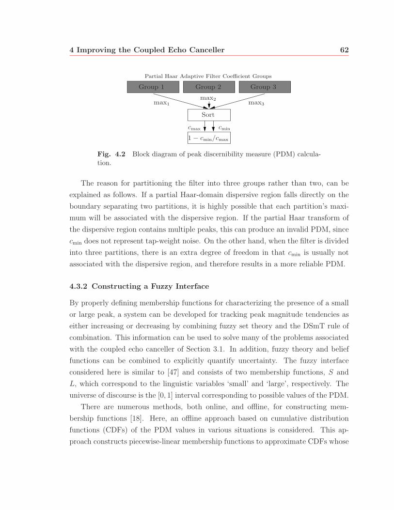
4 Improving the Coupled Echo Canceller 62
Partial Haar Adaptive Filter Coefficient Groups
Group 1 Group 2 Group 3
max1
max2max3
Sort
cmax cmin
1 − cmin/cmax
Fig. 4.2 Block diagram of peak discernibility measure (PDM) calcula-tion.
The reason for partitioning the filter into three groups rather than two, can be
explained as follows. If a partial Haar-domain dispersive region falls directly on the
boundary separating two partitions, it is highly possible that each partition’s maxi-
mum will be associated with the dispersive region. If the partial Haar transform of
the dispersive region contains multiple peaks, this can produce an invalid PDM, since
cmin does not represent tap-weight noise. On the other hand, when the filter is divided
into three partitions, there is an extra degree of freedom in that cmin is usually not
associated with the dispersive region, and therefore results in a more reliable PDM.
4.3.2 Constructing a Fuzzy Interface
By properly defining membership functions for characterizing the presence of a small
or large peak, a system can be developed for tracking peak magnitude tendencies as
either increasing or decreasing by combining fuzzy set theory and the DSmT rule of
combination. This information can be used to solve many of the problems associated
with the coupled echo canceller of Section 3.1. In addition, fuzzy theory and belief
functions can be combined to explicitly quantify uncertainty. The fuzzy interface
considered here is similar to [47] and consists of two membership functions, S and
L, which correspond to the linguistic variables ‘small’ and ‘large’, respectively. The
universe of discourse is the [0, 1] interval corresponding to possible values of the PDM.
There are numerous methods, both online, and offline, for constructing mem-
bership functions [18]. Here, an offline approach based on cumulative distribution
functions (CDFs) of the PDM values in various situations is considered. This ap-
proach constructs piecewise-linear membership functions to approximate CDFs whose
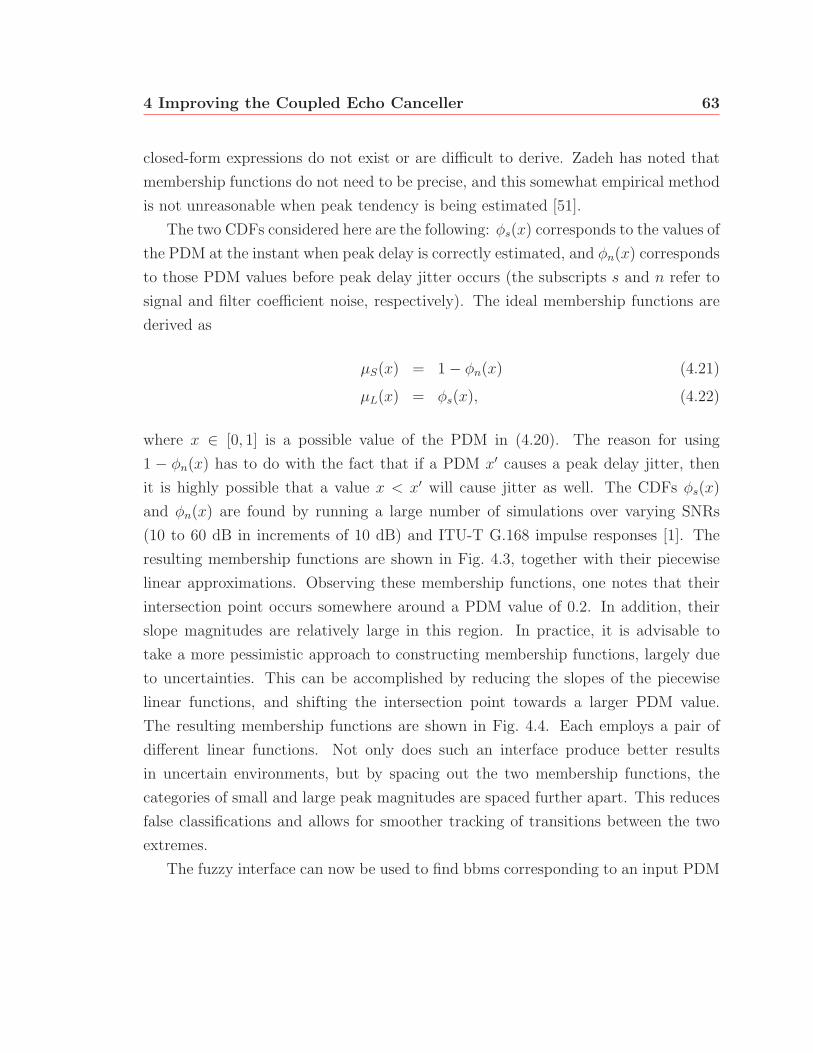
4 Improving the Coupled Echo Canceller 63
closed-form expressions do not exist or are difficult to derive. Zadeh has noted that
membership functions do not need to be precise, and this somewhat empirical method
is not unreasonable when peak tendency is being estimated [51].
The two CDFs considered here are the following: φs(x) corresponds to the values of
the PDM at the instant when peak delay is correctly estimated, and φn(x) corresponds
to those PDM values before peak delay jitter occurs (the subscripts s and n refer to
signal and filter coefficient noise, respectively). The ideal membership functions are
derived as
μS(x) = 1 − φn(x) (4.21)
μL(x) = φs(x), (4.22)
where x ∈ [0, 1] is a possible value of the PDM in (4.20). The reason for using
1 − φn(x) has to do with the fact that if a PDM x′ causes a peak delay jitter, then
it is highly possible that a value x < x′ will cause jitter as well. The CDFs φs(x)
and φn(x) are found by running a large number of simulations over varying SNRs
(10 to 60 dB in increments of 10 dB) and ITU-T G.168 impulse responses [1]. The
resulting membership functions are shown in Fig. 4.3, together with their piecewise
linear approximations. Observing these membership functions, one notes that their
intersection point occurs somewhere around a PDM value of 0.2. In addition, their
slope magnitudes are relatively large in this region. In practice, it is advisable to
take a more pessimistic approach to constructing membership functions, largely due
to uncertainties. This can be accomplished by reducing the slopes of the piecewise
linear functions, and shifting the intersection point towards a larger PDM value.
The resulting membership functions are shown in Fig. 4.4. Each employs a pair of
different linear functions. Not only does such an interface produce better results
in uncertain environments, but by spacing out the two membership functions, the
categories of small and large peak magnitudes are spaced further apart. This reduces
false classifications and allows for smoother tracking of transitions between the two
extremes.
The fuzzy interface can now be used to find bbms corresponding to an input PDM
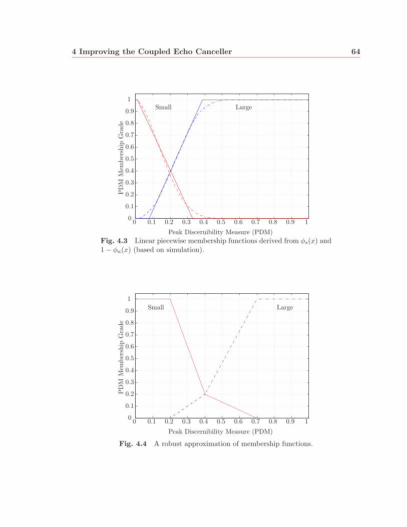
4 Improving the Coupled Echo Canceller 64
0 0.1 0.2 0.3 0.4 0.5 0.6 0.7 0.8 0.9 10
0.1
0.2
0.3
0.4
0.5
0.6
0.7
0.8
0.9
1Small Large
PD
MM
embe
rshi
pG
rade
Peak Discernibility Measure (PDM)Fig. 4.3 Linear piecewise membership functions derived from φs(x) and1 − φn(x) (based on simulation).
0 0.1 0.2 0.3 0.4 0.5 0.6 0.7 0.8 0.9 10
0.1
0.2
0.3
0.4
0.5
0.6
0.7
0.8
0.9
1Small Large
PD
MM
embe
rshi
pG
rade
Peak Discernibility Measure (PDM)
Fig. 4.4 A robust approximation of membership functions.
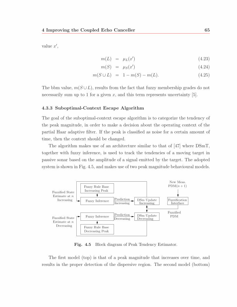
4 Improving the Coupled Echo Canceller 65
value x′,
m(L) = μL(x′) (4.23)
m(S) = μS(x′) (4.24)
m(S ∪ L) = 1 −m(S) −m(L). (4.25)
The bbm value, m(S ∪L), results from the fact that fuzzy membership grades do not
necessarily sum up to 1 for a given x, and this term represents uncertainty [5].
4.3.3 Suboptimal-Context Escape Algorithm
The goal of the suboptimal-context escape algorithm is to categorize the tendency of
the peak magnitude, in order to make a decision about the operating context of the
partial Haar adaptive filter. If the peak is classified as noise for a certain amount of
time, then the context should be changed.
The algorithm makes use of an architecture similar to that of [47] where DSmT,
together with fuzzy inference, is used to track the tendencies of a moving target in
passive sonar based on the amplitude of a signal emitted by the target. The adopted
system is shown in Fig. 4.5, and makes use of two peak magnitude behavioural models.
FuzzificationInterface
FuzzifiedDSm Update
DSm UpdateIncreasingIncreasing Increasing
Decreasing
Decreasing Decreasing
New Meas.
Prediction
Prediction
PDM(n+ 1)
PDMFuzzy Inference
Fuzzy Inference
Fuzzy Rule Base
Fuzzy Rule Base
Fuzzified State
Fuzzified State
Estimate at n
Estimate at n
Decreasing Peak
Increasing Peak
Fig. 4.5 Block diagram of Peak Tendency Estimator.
The first model (top) is that of a peak magnitude that increases over time, and
results in the proper detection of the dispersive region. The second model (bottom)
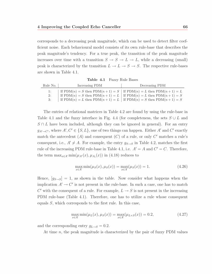
4 Improving the Coupled Echo Canceller 66
corresponds to a decreasing peak magnitude, which can be used to detect filter coef-
ficient noise. Each behavioural model consists of its own rule-base that describes the
peak magnitude’s tendency. For a true peak, the transition of the peak magnitude
increases over time with a transition S → S → L → L, while a decreasing (small)
peak is characterized by the transition L → L → S → S. The respective rule-bases
are shown in Table 4.1.
Table 4.1 Fuzzy Rule BasesRule No. Increasing PDM Decreasing PDM
1: If PDM(n) = S then PDM(n + 1) = S If PDM(n) = L then PDM(n + 1) = L2: If PDM(n) = S then PDM(n + 1) = L If PDM(n) = L then PDM(n + 1) = S3: If PDM(n) = L then PDM(n + 1) = L If PDM(n) = S then PDM(n + 1) = S
The entries of relational matrices in Table 4.2 are found by using the rule-base in
Table 4.1 and the fuzzy interface in Fig. 4.4 (for completeness, the sets S ∪ L and
S ∩ L have been included, although they can be ignored in general). For an entry
gA′→C′ , where A′, C ′ ∈ {S, L}, one of two things can happen. Either A′ and C ′ exactly
match the antecedent (A) and consequent (C) of a rule, or only C ′ matches a rule’s
consequent, i.e., A′ �= A. For example, the entry gS→S in Table 4.2, matches the first
rule of the increasing PDM rule-base in Table 4.1, i.e. A′ = A and C ′ = C. Therefore,
the term maxx∈X min(μA′(x), μAi(x)) in (4.18) reduces to
maxx∈X
min(μS(x), μS(x)) = maxx∈X
(μS(x)) = 1. (4.26)
Hence, [gS→S] = 1, as shown in the table. Now consider what happens when the
implication A′ → C ′ is not present in the rule-base. In such a case, one has to match
C ′ with the consequent of a rule. For example, L→ S is not present in the increasing
PDM rule-base (Table 4.1). Therefore, one has to utilize a rule whose consequent
equals S, which corresponds to the first rule. In this case,
maxx∈X
min(μL(x), μS(x)) = maxx∈X
(μL×S(x)) = 0.2, (4.27)
and the corresponding entry gL→S = 0.2.
At time n, the peak magnitude is characterized by the pair of fuzzy PDM values
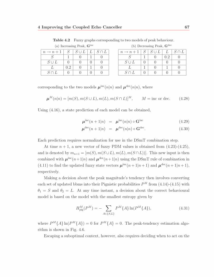
4 Improving the Coupled Echo Canceller 67
Table 4.2 Fuzzy graphs corresponding to two models of peak behaviour.(a) Increasing Peak, Ginc
n→ n+ 1 S S ∪ L L S ∩ LS 1 0 1 0
S ∪ L 0 0 0 0L 0.2 0 1 0
S ∩ L 0 0 0 0
(b) Decreasing Peak, Gdec
n→ n+ 1 S S ∪ L L S ∩ LS 1 0 0.2 0
S ∪ L 0 0 0 0L 1 0 1 0
S ∩ L 0 0 0 0
corresponding to the two models μinc(n|n) and μdec(n|n), where
μM(n|n) = [m(S),m(S ∪ L),m(L),m(S ∩ L)]M , M = inc or dec. (4.28)
Using (4.16), a state prediction of each model can be obtained,
μinc(n+ 1|n) = μinc(n|n) ◦ Ginc (4.29)
μdec(n+ 1|n) = μdec(n|n) ◦ Gdec. (4.30)
Each prediction requires normalization for use in the DSmT combination step.
At time n + 1, a new vector of fuzzy PDM values is obtained from (4.23)-(4.25),
and is denoted by mn+1 = [m(S),m(S ∪L),m(L),m(S ∩L))]. This new input is then
combined with μinc(n+1|n) and μdec(n+1|n) using the DSmT rule of combination in
(4.11) to find the updated fuzzy state vectors μinc(n+ 1|n+ 1) and μdec(n+ 1|n+ 1),
respectively.
Making a decision about the peak magnitude’s tendency then involves converting
each set of updated bbms into their Pignistic probabilities PM from (4.14)-(4.15) with
θ1 = S and θ2 = L. At any time instant, a decision about the correct behavioural
model is based on the model with the smallest entropy given by
HMpig(P
M) = −∑
A∈{S,L}PM{A} ln(PM{A}), (4.31)
where PM{A} ln(PM{A}) = 0 for PM{A} = 0. The peak-tendency estimation algo-
rithm is shown in Fig. 4.6.
Escaping a suboptimal context, however, also requires deciding when to act on the

4 Improving the Coupled Echo Canceller 68
Given : μM (n|n),GM ,M = {inc,dec}.Input : PDM(n + 1).
// new observation: 2 comp., 4+, 2×mn+1(S) = μS(PDM(n + 1));1
mn+1(L) = μL(PDM(n + 1));2
mn+1(S ∪ L) = 1 − mn+1(S) − mn+1(L);3
mn+1(S ∩ L) = 0;4
for each model M = {inc,dec} do5
// prediction-normalization (mpred(S ∪ L) = mpred(S ∩ L) = 0):3 comp., 1+, 1/
μM (n + 1|n) � [mpred(S),mpred(S ∪ L),mpred(L),mpred(S ∩ L)] = μM (n|n) ◦ GM ;6
μM (n + 1|n) = μM (n + 1|n)mpred(S) + mpred(L) ;
7
// state updating using (4.11): 6×, 3+mupd(S) = mpred(S)mn+1(S) + mpred(S)mn+1(S ∪ L);8
mupd(S ∪ L) = 0 mupd(L) = mpred(L)mn+1(L) + mpred(L)mn+1(S ∪ L);9
mupd(S ∩ L) = mpred(S)mn+1(L) + mpred(L)mn+1(S);10
// new state vector
μM (n + 1|n + 1) = [mupd(S),mupd(S ∪ L),mupd(L),mupd(S ∩ L)];11
// Pignistic transform (4.14)-(4.15): 2+, 2×PM{S} = mupd(S) + 0.5mupd(S ∪ L) + 0.5mupd(S ∩ L);12
PM{L} = mupd(L) + 0.5mupd(S ∪ L) + 0.5mupd(S ∩ L);13
// Pignistic entropy (4.31): 1 comp.
HMpig = −PM{S} ln(PM{S}) − PM{L} ln(PM{L});14
end15
Fig. 4.6 Peak-tendency estimation algorithm.
information provided by the above system. Particularly in the case of the partial Haar
adaptive filter, this can prove to be difficult and should be based on the convergence
behaviour of the adaptive filter. This, in turn, depends on a multitude of factors
such as the input statistics, channel conditions, and most importantly, the context
within which the filter is operating. In [24], this time is set to some multiple of the
average time constant of the adaptation algorithm, to give the filter sufficient time to
converge.
The approach developed here is slightly more involved due to the fact that there
are N/q contexts. Therefore, instead of waiting for a certain number of time samples
until the filter converges, the proposed method uses a schedule of N/q waiting times
to sequentially test each context. The waiting times are derived so as to reduce the
4 Improving the Coupled Echo Canceller 69
average time spent waiting for a context that allows for the successful estimation of
a dispersive region’s location.
The above problem, is not unique to suboptimal context escaping, but can be
generalized to a theory of testing a finite set of alternatives. For example, consider
being given a problem with a unique solution S, and a reward R for solving the
problem. Assume there are J different ways this problem can be solved, and each one
leads to this one solution, i.e. all approaches produce the same reward. However, each
approach Aj (j = 1, . . . , J), is associated with a random cost (with respect to time)
Cj with distribution Fj. In other words, each approach requires a different amount
of time to reach the solution. Although the different approaches Aj are known, the
unique mapping M : Ai → Fj between each approach and its corresponding cost
distribution is unknown.
The problem is to find an optimal schedule consisting of J trial periods τ =
{τ1, . . . , τJ} to sequentially attempt each alternative so that the average time spent
reaching the solution is minimized, subject to the constraint that the probability of
eventually finding the solution using this schedule is greater than or equal to some
confidence threshold. The problem is further restricted in that once an alternative
has been attempted without success for a period of time greater than the current trial
period, it is discarded and never revisited again.
Applying the above analysis to suboptimal-context escaping is not straightforward.
The main reason is that not only is the mapping between contexts and their distribu-
tions unknown, but the distributions are also unknown. Therefore, the best that can
be done is to find a schedule based on some prior knowledge about correct estimation
times. In other words, this schedule should ensure that the partial Haar adaptive
filter stay in an optimal context, while only remaining in suboptimal contexts as a
last resort.
A schedule that satisfies the above requirements consists of a sequence of non-
decreasing trial periods, i.e. τ1 ≤ τ2 ≤ . . . ≤ τN . The non-decreasing property is
critical here because the number of contexts that can successfully lead to a correct
estimate of the peak delay should increase after each failed attempt. At the same time,
beginning the schedule with shorter waiting times escapes any suboptimal contexts
earlier in the peak delay estimation process, while at the same time successfully staying
4 Improving the Coupled Echo Canceller 70
in optimal contexts.
The individual trial times or periods of the scheduling policy remain to be deter-
mined. The first trial period should be related to the number of samples required
to properly detect the global peak in an optimal context. As will be seen in Chap-
ter 5, optimal contexts usually require less than a 200 samples to correctly detect a
peak using an NLMS algorithm with a step-size μ = 1 and a sampling rate of 8 kHz.
Therefore, the first trial period can be set to approximately 150 samples.
Setting the final trial period (N/q) is usually based on the amount of time willing
to be spent operating in a worst-case context. This time period should not be set too
long, and can be set somewhere between 400–500 samples. The remaining trial periods
can be uniformly distributed between the minimum and maximum trial periods. To
summarize, the algorithm begins by monitoring the peak tendency using the smallest
trial period. If the peak tendency is classified as decreasing for a period of time
greater than this trial period and jitter occurs in the peak delay estimate, then the
filter is reset to zero and a new context is attempted for the next trial period. This is
repeated until the peak delay is correctly estimated. One issue has been ignored,
and that is what happens when none of the contexts provide a correct peak using the
given schedule? The approach used here re-tests all contexts in the same order as the
previous test, beginning with the second-shortest trial time. The suboptimal-context
escape algorithm is shown in Fig. 4.7.
4.4 Improved Tracking of the Partial Haar Adaptive Filter
In Section 3.2.2, the tracking of a dispersive region after an abrupt change in the echo
path impulse response was seen as a competition between filter coefficient magnitudes.
Changes in an echo path impulse response can be associated with a change in the bulk
delay, or a phase roll, where the impulse response coefficients change signs [50].
When the partial Haar adaptive filter is initialized to zero, a peak’s magnitude
only has to compete with the low-magnitude coefficient noise of the surrounding taps,
which makes its detection easy and fast. In the event of an abrupt change in the
echo path impulse response, however, a new peak might have to compete with the
decreasing magnitude of an old peak. Therefore, although the echo path impulse

4 Improving the Coupled Echo Canceller 71
Given: H incpig and Hdec
pig from peak tendency estimator (see Fig. 4.6),schedule, τ = {τ1, τ2, . . . , τN/q},partial Haar peak indices at times n and n + 1: index(n), index(n + 1),peak-tendency counters: counter inc and counter dec,context variable, context.
Initial: (at n = 0), counter inc = counter dec = 0, k = 1, T = τ1, context = 1, v(n) = 0.
// at time n + 1 . . .
if Hdecpig < H inc
pig then1
counter dec = counter dec + 1;2
else3
counter inc = counter inc + 1;4
end5
// if the current trial time is exceeded and peak jitter occurs// ∧ denotes the logic-and operation and mod(·) the modulus operationif (counter dec ≥ T ) ∧ (|index(n + 1) − index(n)| > 10) then6
v(n + 1) = 0;7
k = min(k + 1, N/q);8
T = τk;9
context = mod(context, N/q) + 1;10
// re-testing if all trial times have failedif k == N/q then11
k = 1;12
end13
counter dec = 0;14
counter inc = 0;15
end16
// schedule and counter resettingif counter inc ≥ T then17
k = 1;18
T = τ1;19
counter dec = 0;20
counter inc = 0;21
end22
Fig. 4.7 Suboptimal-Context Escape Algorithm.
4 Improving the Coupled Echo Canceller 72
response has changed, the peak delay estimator will take longer to locate the peak
corresponding to the new impulse response. The goal of this section is to reduce the
amount of time it takes the peak delay estimator to track new dispersive regions in
these situations.
One of the key properties of the coupled echo canceller structure in Fig. 3.1 is
that the partial Haar filter is not being used to actually cancel echo. This allows
some degree of flexibility in manipulating the operation of the filter, particularly for
purposes of enhanced tracking performance.
Analyzing equations (3.33) and (3.34) in the event of a change in the echo path
impulse response, one finds that although the location of the new peak as well as
its steady-state magnitude is unknown, the new steady-state magnitude of an old
peak is approximately zero. Therefore, if a decrease in the current peak’s magnitude
is detected (which usually signals a change in the echo path impulse response), it
may be simpler to reset the whole partial Haar filter to v(n) = 0. This allows
for the new peak to solely compete with the low-magnitude coefficient noise of its
neighbouring taps instead of the decreasing magnitude of the previous peak. As a
result, the performance gains shown by Bershad and Bist [4] in the stationary case
can be extended to cases where abrupt changes in the echo path impulse response
occur.
In order to prevent the algorithm from constantly resetting the partial Haar adap-
tive filter, the reset operation should only be performed every TRS samples. In addi-
tion, a reset is only deemed necessary when a decrease in magnitude is detected for
a peak whose tendency has been in an increasing state for an amount of time greater
then Tinc. It is usually the case that TRS < Tinc.
One remaining problem, however, is that the improved tracking algorithm might
falsely detect a change in the impulse response. This is due to the stochastic driving
force φk(n) in (2.40) that causes the filter coefficients to display a form of Brownian
motion around the optimal solution [22, 36]. In order to prevent these false alarms, the
algorithm cannot simply reset the filter to zero. Instead, it also stores the position of
the previous peak before resetting the filter, and feeds this position to the bulk delay
unit. Once the new peak tendency has been increasing for an amount of time equal to
Tinc, the algorithm uses the location of the new peak to centre the short time-domain
4 Improving the Coupled Echo Canceller 73
filter. The value of Tinc is set so as not to cause jitter in the peak delay estimate being
fed to the bulk delay in the case of a false alarm.
Figure 4.8 shows the improved tracking algorithm combined with the suboptimal-
context escaping algorithm.
4.5 Distributed Peak Detection for Cancellation of Multiple
Echoes
Cancellation of multiple echoes can be a difficult task, particularly since no prior
information is available concerning the number of dispersive regions. The method
proposed here is based on a coordinator-multi-agent architecture similar to [10].
The proposed multiple echo canceller is based on two assumptions,
1. There is an average bound on the length of dispersive regions in the time domain.
2. The delay between reflections is larger than this upper bound so that almost no
overlap occurs between the dispersive regions of the channel impulse response.
The first assumption is reasonable and is backed by empirical data [1]. Most network
hybrid impulse responses range from 3–12 ms, or a corresponding length of 24–96
samples at a sampling rate of 8 kHz [1]. To simplify the current analysis and the
ensuing simulations in Chapter 5, the length of the dispersive region will be taken
as L = 128 samples at 8 kHz, which is the assumed length of the short time-domain
filter. The second assumption prevents problems where a delay between echoes is
such that there is a 30–50 percent overlap between dispersive regions, in which case
assumption one is violated, since the combined echoes can interpreted as one longer
dispersive region. A block diagram of the multiple echo canceller is shown in Fig. 4.9.
The partial Haar adaptive filter is divided into N/L partitions, each of length
qL/N , where L is the expected length of a dispersive region in the time-domain
(as well as the length of the short time-domain adaptive filter). Associated with each
partition is a region that overlaps with its left-hand neighbouring partition. Of course,
the first (leftmost) region simply corresponds to that partition.
The amount of overlap is set so as to create a region-length that is divisible by
3. The second assumption stated at the beginning of this section ensures that at

4 Improving the Coupled Echo Canceller 74
Given: See given data in Fig. 4.7,rerouting variables peak reroute, TRS , Tinc and counter,maximum-magnitude tap-weight at time n + 1, vmax(n + 1),current overall maximum tap-weight magnitude and position, max peak andmax index.
Initial: (at n = 0), v(0) = 0, counter inc = counter dec = 0, k = 1, T = τ1, context = 1,max peak = 0, max index = 1.
// at time n + 1 . . .insert : lines 1-16 from Fig. 4.7
// schedule and counter resettingif counter inc ≥ T then
k = 1;T = τ1;
end
// re-routing of peak location: old vs. newif (peak reroute == 1) ∧ (counter inc < Tinc) then // use old peak position
index(n + 1) = max index;else // use new peak position
peak reroute = 0;counter = counter + 1;
end// poll the maximum peak magnitude for any decreaseif counter ≥ TRS then
counter = 0;if |vmax| ≥ max peak then
max peak = |vmax|;endif (|vmax| < max peak) ∧ (counter inc ≥ Tinc) then
peak reroute = 1;k = 1;T = τ1;counter dec = 0;counter inc = 0;v(n + 1) = 0;max index = index(n + 1);max peak = 0;
endend
Fig. 4.8 Improved tracking algorithm with suboptimal-context es-caping.
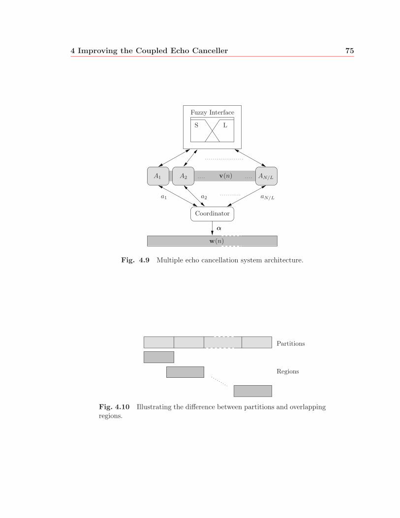
4 Improving the Coupled Echo Canceller 75
Fuzzy Interface
S L
Coordinator
A1 A2 AN/L
a1 a2 aN/L
v(n)
w(n)
α
Fig. 4.9 Multiple echo cancellation system architecture.
Partitions
Regions
Fig. 4.10 Illustrating the difference between partitions and overlappingregions.
4 Improving the Coupled Echo Canceller 76
most one dispersive region can be located within any given region. The reason for
including such a constraint will become clearer later when the issue of dispersive
regions occurring near boundaries of partitions is considered. The difference between
partitions and regions is shown in Fig. 4.10.
For example, in the case of a length N = 1024 time-domain filter (see Fig. 4.9)
and corresponding partial Haar filter of length q = 256, the number of partitions
is N/L = 1024/128 = 8 where each partition is of length q/8 = 256/8 = 32. To
make the region-lengths divisible by 3, each region contains its respective partition
and 7 samples from its left-hand neighbour’s partition, resulting in a region length of
32 + 7 = 39 which is divisible by 3.
Associated with each region is an agent Ai that runs a distributed version of the
suboptimal-context escape algorithm. Although similar to the single-echo version of
the algorithm, the distributed form departs slightly in its calculation of the PDM,
which is given by
PDMi = 1 − min(ci max, c)
ci max
. (4.32)
Unlike the case of a single dispersive region in Section 4.3.3, each agent sends ci min
to the coordinator (see Fig. 4.9) where c is calculated as c = maxi ci min. The term
min(ci max, c) is necessary because c > ci max in some cases, making the original PDM
negative. Part of the motivation for using cooperative, rather than independent agents
has to do with conserving the global characteristic of the PDM.
Escaping suboptimal contexts is complicated by the presence of multiple echoes,
since each agent has control over only a finite number of tap weights. Therefore,
if a certain agent requires a context switch, only its corresponding partition’s con-
text should be changed. This is where the efficient calculation of the partial Haar
coefficients from Section 4.1 comes into play, since each set of coefficients is readily
available.
In case a peak occurs near a boundary between two partitions, it would be neces-
sary for the two partitions sharing this boundary to remain in the same context. This
is because depending on the contexts at the boundary of two partitions, the partial
Haar transform matrix can lose its row-orthogonality, since basis functions can over-
lap at these boundaries depending on the contexts selected. There are two cases that
can result from two neighbouring partitions operating in different contexts.

4 Improving the Coupled Echo Canceller 77
In the first case, the context number of an agent’s partition is greater than or
equal to the context number of its left neighbour, in which case no overlap occurs at
the boundary. In the second case, the context number is less than its left neighbour’s
number, resulting in overlap and smearing of the transformed Wiener solution in (3.4)
at the boundary. Therefore, overlapping regions ensure the same operating context
for two contiguous agents that share a peak near their boundary.
PeakDiscernibility
Measure
PeakTendencyEstimation
Active/Inactive
Fig. 4.11 Multiple echo cancellation agent architecture.
Figure 4.11 shows the architecture of each agent, which consists of three stages
that are repeated every iteration. The first step consists of calculating the PDM
associated with the peak located in each agent’s region. Depending on the dominant
peak behavioural model, each agent is classified as active or inactive. This information
is stored in a length-N/L indicator vector a of active agents. If ai = 1, then agent Ai
is classified as active; otherwise if ai = 0, the agent is deemed inactive. If agent i’s
peak tendency has been in an increasing state for more than Tinc samples, then ai is
set to 1, and the agent is classified as active. Tinc, is used to prevent false or transient
classifications of agents.
Using information about the state of an agent (active or inactive), the central
coordinator does one of two things. If none of the agents are active, i.e. ai = 0 for
all i, then the coordinator signals for all N time-domain adaptive filter coefficients
to be updated. If, however, at least one of the agents is active, then the coordinator
uses the peak locations of those agents to update only certain tap-weights of the
time-domain adaptive filter. The activated tap-weights are centred around the peak
delay estimates provided by each of the active agents. Therefore, the NLMS update
equation of the time-domain adaptive filter is modified to
w(n+ 1) = diag(α)[w(n) +μ
‖diag(α)u(n)‖2 e(n)u(n)]. (4.33)

4 Improving the Coupled Echo Canceller 78
where α is a length-N indicator vector whose elements αi are used to either activate
specific regions of the time-domain adaptive filter, or to simply update the entire
adaptive filter.
Unfortunately, the improved tracking algorithm in Section 4.4 cannot be incorpo-
rated into the multiple echo canceller. In the case of multiple echo cancellation, a
Given: Tinc, τ = {τ1, τ2, . . . , τN/q},For each agent j,
peak indices at times n and n + 1: index(j, n), index(j, n + 1)contexts: context(j)peak-tendency counters: counter inc(j) and counter dec(j).
Initial: (at n = 0), counter inc(j) = counter dec(j) = 0, k(j) = 1, T (j) = τ1,context(j) = 1 for all j.
// at time n + 1 . . .the coordinator returns c from the broadcasted values ci min of each agent ;a = 0N/L;α = 0N ;for each of the N/L agents do
calculate PDM(n + 1) according to (4.32);insert : code from Fig. 4.6insert : lines 1-16 from Fig. 4.7
if counter inc(j) ≥ T (j) thenk(j) = 1;T (j) = τ1;
end// activate or deactivate an agentaj = 0;if counter inc(j) ≥ Tinc then
aj = 1;set the appropriate elements of α to 1 using (3.39);
endend
// if none of the agents are activatedif
∑ai == 0 then
α = 1;end
use (4.33) to update the time-domain adaptive filter ;
Fig. 4.12 Multiple echo canceller.
detected change in the current peak can also be associated with the disappearance of
the current reflection in the given parition. Therefore, resetting a single partition is
not feasible.
79
Chapter 5
Simulation Results and Discussion
Chapters 3 and 4 looked at the major drawbacks of the echo canceller introduced by
Bershad and Bist [4], and proposed feasible solutions to these problems. The current
chapter uses simulation experiments to build upon these critiques and proposals in
two ways. First, it exemplifies the argued pitfalls of the original system, which include
convergence and tracking issues. At the same time, the merits of the proposed algo-
rithms in tackling these issues are shown. In addition to simulations, this chapter also
analyzes the computational complexities of two of the main algorithms in Chapter 4.
5.1 Experimental Methodology
The following section introduces simulation parameters and the various filtering algo-
rithms that will be used to compare with the algorithms proposed in Chapter 4.
5.1.1 Simulation Data
The set of hybrid impulse responses used in the following simulations are taken from
Annex D of the ITU-T G.168 Recommendation for digital network echo cancellers
[1]. There are eight hybrid impulse responses mi(n) (for i = 1, 2, . . . , 8) of lengths
Li that range from 64 to 128 samples at 8 kHz. It is assumed that mi(n) = 0 for
n /∈ {0, 1, . . . , Li − 1}. Impulse responses i = 1 to 4 were generated from a network
hybrid simulator, while the last four consist of measured impulse responses from
telephone networks in North America.
2006/09/28
5 Simulation Results and Discussion 80
The echo path impulse responses g(n) are generated according to [1]
g(n) = (10−ERL/20ki)mi(n− Δ), (5.1)
where ERL is the echo return loss, ki is a scaling factor that depends on mi(n), and Δ
represents the bulk delay. In addition, the Recommendation provides guidelines for
testing echo cancellers, which includes different values of various parameters including
the ERL. For the purpose of the presented simulations an ERL of 15 dB will be
assumed for all hybrid impulse responses. Furthermore, ERL is not adjusted with
bulk delay so as not to over-complicate the discussion. The value of Δ will be set
so that the length of the bulk delay plus the dispersive region does not exceed 1024
samples.
The length of the partial Haar adaptive filter will be q = 256, unless stated
otherwise. Longer filters (q = 512) will not be considered here since their use is
computationally expensive, while the resulting performance of shorter filters is simply
not up to par with intermediate cases (q = 128 or 256). The short time-domain
adaptive filter length is set to L = 128 to match the longest dispersive region. When
using a full time-domain adaptive filter in the multiple echo case, its length is set to
N = 1024 to match the longest possible echo path impulse response.
The input u(n) is a zero-mean Gaussian process with unit variance. The additive
measurement noise ν(n) is also a white Gaussian process of zero-mean and variance
σ2ν = 10−SNR/10. The samples of ν(n) are also assumed to be uncorrelated with the
input. The SNR is set to 30 dB, unless stated otherwise. All simulation data and
programs were generated and written in MATLABR©.
A note should be made concerning the terms ‘optimal’, ‘best’, ‘suboptimal’, and
‘worst’ associated with the partial Haar adaptive filter’s (shift) context. Optimal and
suboptimal contexts correspond to those combinations of contexts and bulk delays
that produce fast and slow localizations of dispersive regions, respectively. The best
and worst contexts of a given impulse response produce the fastest and slowest lo-
calization of a dispersive region, respectively. The above categories will only be used
when the input is uncorrelated and Gaussian, and are obtained by applying the N/q
shifted-versions of the partial Haar transform to an echo path impulse response of
interest. The contexts can then be sorted according to the resulting partial Haar

5 Simulation Results and Discussion 81
peak magnitudes, where the largest magnitude corresponds to the best context, for a
given impulse response.
5.1.2 Adaptive Filtering Algorithms
The original coupled echo canceller, which is also termed the partial Haar dual adap-
tive filter in [4], will be abbreviated as PHDAF. When validating the performance of
each of the proposed improvements, different filtering algorithms will be used used
for comparison. Of course, deciding which algorithms to benchmark against depends
on which modification is being tested.
When testing the merits of escaping suboptimal contexts, the proposed suboptimal-
context escape algorithm (SCE-PHDAF) will be compared to both the PHDAF, in
addition to the NLMS. In this case, the NLMS will simply serve as a reference. In
the case of studying the performance of the improved tracking algorithm with sub-
optimal context escaping (IT-PHDAF), the learning curves of the IT-PHDAF will be
compared to both the PHDAF and NLMS.
Although the PHDAF does not support multiple echoes, the multiple echo can-
celler’s (ME-PHDAF) performance will be compared to it in the case of a single echo.
In addition to comparing the ME-PHDAF to the NLMS algorithm, an ideal-NLMS
(INLMS) algorithm will also be used to provide an optimal performance bound on
the ME-PHDAF for the multiple echo case. The INLMS algorithm is the standard
NLMS algorithm, except in that it adapts only those filter coefficients centred around
the locations of the true impulse response’s dispersive regions. This corresponds to
the case where prior knowledge about the echo locations exists.
The step-size used here is μ = 1 for all forms of the NLMS algorithm (these include
all forms of the partial Haar adaptive filter, the INLMS, and short-time domain filters),
and corresponds to the optimal step-size of the NLMS algorithm. At the beginning
of each run, the input data vector is initialized with the first N input samples.
Concerning the calculation of the normalizing factor ‖u(n)‖2 in Section 3.3.2, some
remarks are in order. First, this power term is calculated using an efficient recursion
on the input data block
‖u(n)‖2 = ‖u(n− 1)‖2 − u2(n−N) + u2(n). (5.2)

5 Simulation Results and Discussion 82
The above equation may suffer from linear error buildup as n increases. However, for
the purposes of these simulations, it was found that the simulation lengths used were
not sufficiently long enough to cause instability.
5.2 Suboptimal-Context Escaping
Studying suboptimal-context escaping requires the use of specific examples, in addi-
tion to simulations that can reliably support the merits of using the SCE-PHDAF in
general. The simulations shown below all use an input data vector of length N = 1024
with a partial Haar adaptive filter of length q = 256 and a schedule (see 4.3.3),
τ = {150, 250, 300, 400}. The NLMS algorithm is used as a basis of comparison
for both the proposed algorithm and PHDAF. The initial context is set to 1, which
corresponds to no shifting of the partial Haar basis vectors.
5.2.1 Specific Cases
Figures 5.1(a) and (b) show the learning curves corresponding to an echo path impulse
response using ITU-T G.168 hybrid model m5(n) under the best and worst bulk delays
(for the initial context), respectively. The curves represent an ensemble of 200 runs
for each simulation.
For the best-case bulk delay (Fig. 5.1(a)), both the SCE-PHDAF and PHDAF
show identical learning curves reaching steady state at around k = 750 compared to
the NLMS which converges at around k = 5000. Of course, this is related to the fact
that the NLMS adapts a far larger number of coefficients (1024 compared to 128). In
the case of a worst-case bulk delay (Fig. 5.1(b)), the PHDAF never seems to reach
steady-state, while the proposed SCE-PHDAF converges much faster, nearly as well
as in the optimal case, requiring about k = 1000 samples to converge.
5.2.2 General Case
The previous learning curves have shown promising performance gains for the SCE-
PHDAF in specific cases. However, to fully accept the above results requires a more
exhaustive test. Figure 5.2 shows the learning curves averaged over a thousand dif-
ferent echo path impulse responses. Each run randomly selects one of eight ITU-T

5 Simulation Results and Discussion 83
G.168 hybrid impulse response with equal probability, and uniformly selects a bulk
delay in the interval [0,895]. The performance of the proposed echo canceller does
not appear as impressive as in the specific cases, although it is still faster than the
PHDAF. Again, the NLMS performs the poorest of all.
In addition to learning curves, the mean time for each echo canceller (proposed and
PHDAF) to correctly estimate the location of a dispersive region was compared for
different SNRs. Each row in Table 5.1 consists of the average and standard deviation
over 500 random runs similar to the general case. In all cases, the proposed algorithm
finds the dispersive region faster (the mean time is smaller) and more consistently (the
standard deviation is much smaller). Although both PHDAF and the proposed echo
canceller display similar mean times to convergence at very low SNR, the standard
deviation of the PHDAF is three times larger.
5.2.3 Discussion
Three major observations need to be made concerning the results in Figs. 5.1-5.2.
First, the specific simulations in Fig. 5.1 show that the proposed algorithm adds
flexibility to the PHDAF in that it does not get trapped in suboptimal contexts. At
the same time the proposed algorithm remains in optimal contexts. This behaviour
may significantly increase the convergence speed of the echo canceller, as observed.
Second, the results in Fig. 5.2 also provide additional insights into the wavelet
transform. It turns out that out of the 1000 runs, only 6.4% actually consisted of a
worst-case combination of bulk delay and hybrid impulse response. This explains why
the PHDAF and the proposed algorithm’s learning curves in Fig. 5.2 are somewhat
similar. However, in specific cases, like Fig. 5.1(b), the difference between the PHDAF
and SCE-PHDAF is substantial, with the SCE-PHDAF showing great improvements.
Finally, Table 5.1 reveals the robustness of using a fixed schedule τ together with
a peak tendency estimator for different values of SNR. Of course, if the SNR does not
change much over a specific channel, then schedules can be constructed specifically
for those cases.
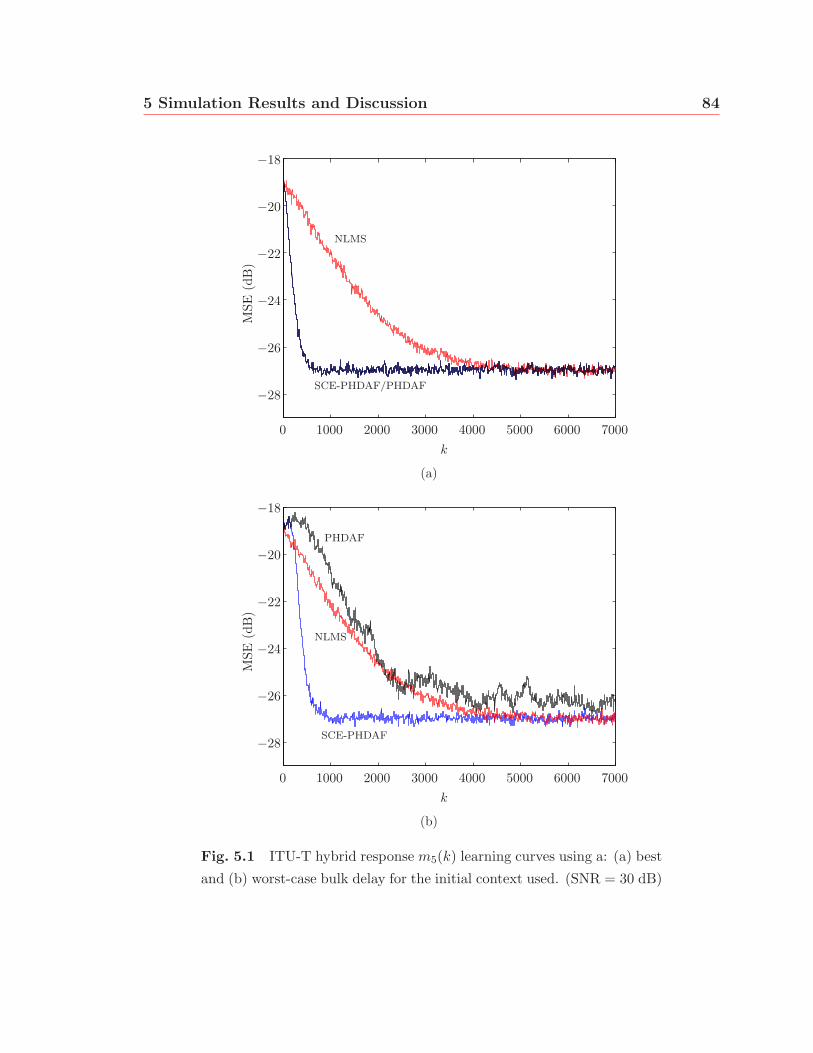
5 Simulation Results and Discussion 84
0 1000 2000 3000 4000 5000 6000 7000
−28
−26
−24
−22
−20
−18
SCE-PHDAF/PHDAF
k
MSE
(dB
)NLMS
(a)
0 1000 2000 3000 4000 5000 6000 7000
−28
−26
−24
−22
−20
−18
SCE-PHDAF
PHDAF
k
MSE
(dB
)
NLMS
(b)
Fig. 5.1 ITU-T hybrid response m5(k) learning curves using a: (a) best
and (b) worst-case bulk delay for the initial context used. (SNR = 30 dB)

5 Simulation Results and Discussion 85
0 1000 2000 3000 4000 5000 6000 7000
−28
−26
−24
−22
−20
−18
−16
−14
NLMS
SCE-PHDAF
PHDAF
k
MSE
(dB
)
Fig. 5.2 Learning curves over 1000 runs, with randomly-selected
(equiprobable) hybrid impulse responses and uniformly-selected bulk de-
lays. (SNR = 30 dB)
Table 5.1 Comparison of mean times and standard deviation to cor-
rectly estimate the peak delay for different SNRs.
SCE-PHDAF PHDAF
SNR (dB) Mean Std. Mean Std.
30 91.5 75.4 121.1 203.0
20 107.7 86.4 214.5 664.0
15 167.4 138.3 362.7 1067.7
10 421.4 387.1 531.7 1177.2
5 Simulation Results and Discussion 86
5.3 Improved Tracking of Changes in an Echo Path
The simulations described below consist of four scenarios where an abrupt change in
the bulk delay, and possibly the hybrid impulse response occurs around time k = 5200.
The waiting periods TRS and Tinc are set to 32 and 128 samples, respectively. Again,
the initial context in Fig. 4.8 is set to 1. Each scenario is categorized according to the
optimality of its bulk delays (before and after the change) with respect to the initial
shift context. For example, ‘best-to-best’ denotes a change from a best bulk delay
to another best-case bulk delay relative to the initial context. The adaptive filtering
parameters are the same as in the previous section.
5.3.1 Results
Best-to-best (Fig. 5.3(a)): Initially, both proposed IT-PHDAF and PHDAF converge
very fast, similar to the previous section. However, after an abrupt change in bulk
delay occurs, the IT-PHDAF resets the partial Haar filter, resulting in a convergence
rate similar to the initial case. In contrast, the PHDAF requires almost 1500 samples
to converge.
Worst-to-worst(Fig. 5.3(b)): Again, the IT-PHDAF converges quickly both ini-
tially and after a change in bulk delay, while the convergence characteristics of the
PHDAF are poor in both stages.
Best-to-worst(Fig. 5.4(a)): Initially, both echo cancellers converge optimally. How-
ever, after the abrupt change in bulk delay, the PHDAF requires much more time to
begin to converge after a sudden change in the bulk delay. This plateau-region ex-
tends for almost 2000 samples as compared to only about 1000 samples in Fig. 5.3(a).
The IT-PHDAF, on the other hand, converges faster and its learning curve behaves
similarly to the case in Fig. 5.3(a).
Worst-to-best(Fig. 5.4(b)): Again, the initial learning curves’ behaviour is similar
to the initial case in Fig. 5.3(b). However, at the transition point, the IT-PHDAF is
slightly slower than the PHDAF, although both converge very quickly (requiring less
than 1000 samples).

5 Simulation Results and Discussion 87
5.3.2 Discussion
The above results can be explained using the theory presented in Section 3.2.2. Only
the behaviour at the transition points will be discussed since the initial behaviours
were already explained in Section 5.2.
In Figures 5.3(a) and 5.4(a), the PHDAF’s learning curve exhibits a plateau after
the change in bulk delay. The length of this plateau equals the amount of time it takes
the new peak’s magnitude to exceed the decreasing magnitude of the old peak. The
plateau region is slightly longer in Fig. 5.4(a) (which corresponds to a best-to-worst
transition) because the time required by the peak delay estimator to track the new
peak (which is very small) equals the amount of time it takes the old peak to become
buried in coefficient noise, unlike the case in Fig. 5.3(a) where a new peak emerges
while the old peak is decreasing. This can also be explained using (3.37), where β ≈ 0
for the abrupt change in Fig. 5.4(a), and therefore, tracking this change takes longer.
In both of the above cases, the IT-PHDAF converges much faster because it resets
the partial Haar adaptive filter once it detects a decrease in old peak’s magnitude.
Its converge time is still not as fast as in the initial case, however, because of Tinc. To
elaborate, the new peak has to be categorized as increasing for Tinc samples before its
index is accepted. During this time, the bulk delay unit continues to use the old peak
location to offset the short time-domain filter.
In the worst-to-worst case of Fig. 5.3(b), it is interesting to observe that the
PHDAF’s learning curve does not exhibit a plateau as in Fig. 5.3(a). The reason
for this, is that since the initial bulk delay is a worst-case delay, there is not much
competition between the peak magnitudes before and after the transitions, and so
they behave similarly.
In the final worst-to-best case, the PHDAF converges slightly faster after the
abrupt change in bulk delay than the proposed algorithm. The reason is that a worst-
case context is almost equivalent to a filter initialized to zero, i.e. v(n) ≈ 0. Once
the bulk delay changes to an optimal value with respect to the initial context, the
emergence of a new peak does not have to compete with the presence of an old peak.
There are two reasons why the IT-PHDAF requires a slightly longer amount of
time to converge in the worst-to-best case. First, the improved tracking algorithm
requires that a new peak’s tendency be in an increasing state for Tinc samples until
5 Simulation Results and Discussion 88
it switches to the new peak’s location. And second, the context escaping algorithm
initially makes a context switch in response to the worst-case bulk delay. After the
abrupt change in echo path impulse response, the new context might not be optimal
with respect to the new bulk delay as the initial context.
5.3.3 Computational Complexity
The bulk of the suboptimal-context escaping and improved tracking algorithms’ com-
putational complexity lie with the peak tendency estimator of Fig. 4.6. Table 5.2
shows the number of arithmetic operations per iteration required by the peak ten-
dency estimator, the suboptimal-context escaping echo canceller, and the improved
tracking echo canceller (which includes suboptimal-context escaping). Since only the
incremental increase in complexity over the PHDAF is of interest here, the complexity
values of the first three columns of Table 5.2 (PTE SCE-PHDAF, IT-PHDAF) do not
include the complexity associated with the PHDAF. The values in the second and
third columns of Table 5.2 include the respective values corresponding to the peak
tendency estimator. The last column is used as a reference to compute the percent-
age increase of incorporating either suboptimal-context escaping or improved tracking
algorithms into the PHDAF.
Arithmetic operations associated the the PTE can be reduced drastically since
many bbm terms such as mn+1(S ∩L), mpred(S ∪L), mpred(S ∪L), mpred(S ∩L), and
mupd(S ∩L) (see Fig. 4.6) are zero throughout the PTE’s operation. Calculating the
new PDM value requires one division and addition operation. The remaining number
of arithmetic operations are shown in Fig. 4.6 for each stage.
It appears that calculating the Pignistic entropies in (4.31) requires the use of
two logarithm operations which are computationally expensive. However, the SCE-
PHDAF and IT-PHDAF only need to measure the peak tendency (see line 15 of
Fig. 4.7), which only involves a comparison of the Pignistic entropies H incpig and Hdec
pig .
This calculation makes no direct use of the actual values. Therefore, an alternate mea-
sure that preserves the relationship between the two Pignistic entropies and requires
only a single comparison operation is given by
HMpig = min(PM{S}, PM{L}), M = {inc, dec}. (5.3)
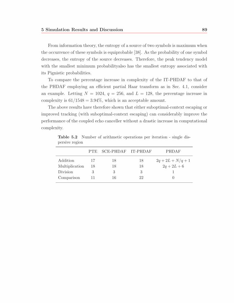
5 Simulation Results and Discussion 89
From information theory, the entropy of a source of two symbols is maximum when
the occurrence of these symbols is equiprobable [38]. As the probability of one symbol
decreases, the entropy of the source decreases. Therefore, the peak tendency model
with the smallest minimum probabilityalso has the smallest entropy associated with
its Pignistic probabilities.
To compare the percentage increase in complexity of the IT-PHDAF to that of
the PHDAF employing an efficient partial Haar transform as in Sec. 4.1, consider
an example. Letting N = 1024, q = 256, and L = 128, the percentage increase in
complexity is 61/1548 = 3.94%, which is an acceptable amount.
The above results have therefore shown that either suboptimal-context escaping or
improved tracking (with suboptimal-context escaping) can considerably improve the
performance of the coupled echo canceller without a drastic increase in computational
complexity.
Table 5.2 Number of arithmetic operations per iteration - single dis-persive region
PTE SCE-PHDAF IT-PHDAF PHDAF
Addition 17 18 18 2q + 2L + N/q + 1Multiplication 18 18 18 2q + 2L + 6Division 3 3 3 1Comparison 11 16 22 0
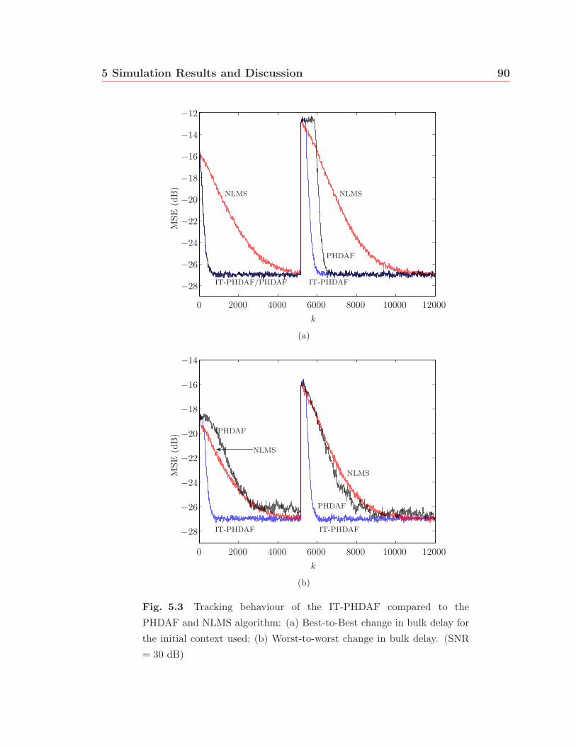
5 Simulation Results and Discussion 90
0 2000 4000 6000 8000 10000 12000
−28
−26
−24
−22
−20
−18
−16
−14
−12
NLMSNLMS
IT-PHDAF
PHDAF
IT-PHDAF/PHDAF
k
MSE
(dB
)
(a)
0 2000 4000 6000 8000 10000 12000
−28
−26
−24
−22
−20
−18
−16
−14
NLMS
NLMS
IT-PHDAF IT-PHDAF
k
MSE
(dB
) PHDAF
PHDAF
(b)
Fig. 5.3 Tracking behaviour of the IT-PHDAF compared to the
PHDAF and NLMS algorithm: (a) Best-to-Best change in bulk delay for
the initial context used; (b) Worst-to-worst change in bulk delay. (SNR
= 30 dB)
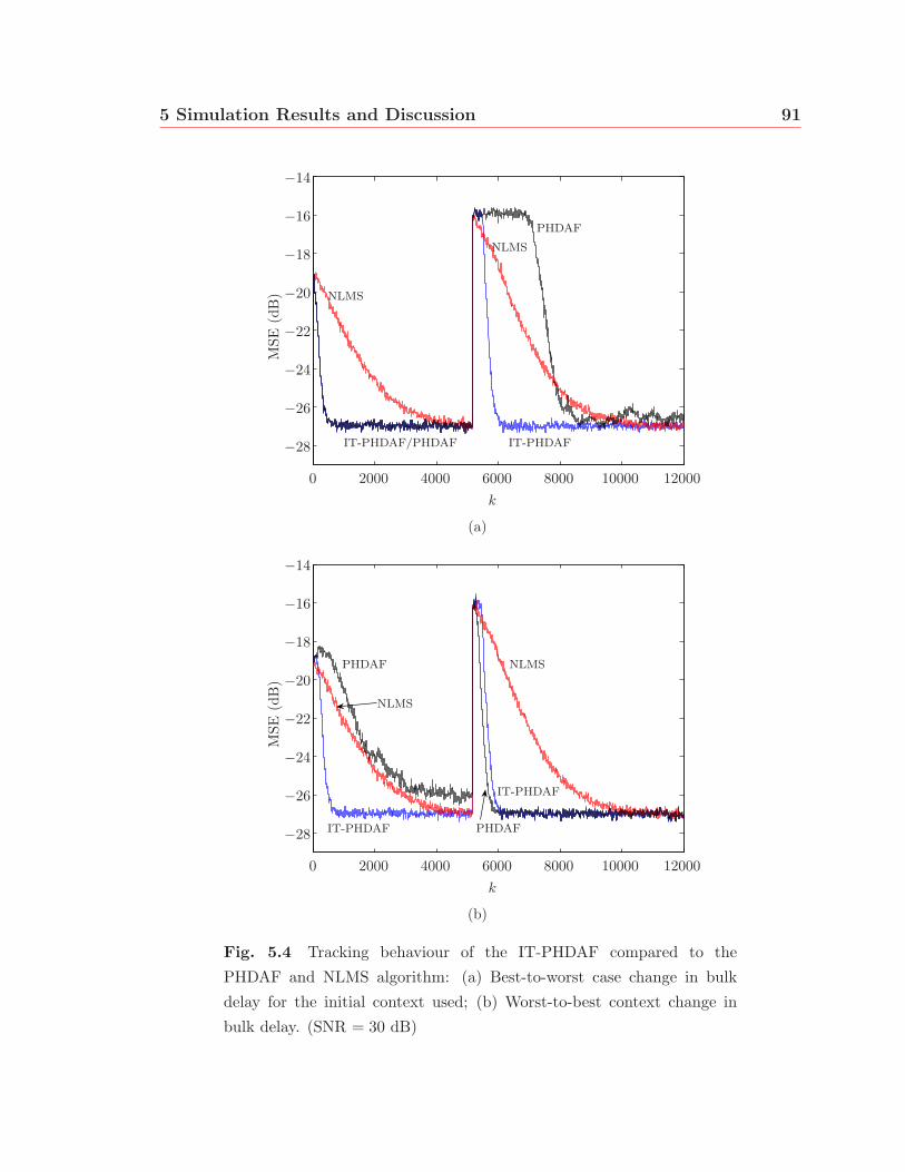
5 Simulation Results and Discussion 91
0 2000 4000 6000 8000 10000 12000
−28
−26
−24
−22
−20
−18
−16
−14
PHDAF
IT-PHDAF/PHDAF
k
MSE
(dB
) NLMS
NLMS
IT-PHDAF
(a)
0 2000 4000 6000 8000 10000 12000
−28
−26
−24
−22
−20
−18
−16
−14
PHDAF
PHDAF
k
MSE
(dB
)
NLMS
NLMS
IT-PHDAF
IT-PHDAF
(b)
Fig. 5.4 Tracking behaviour of the IT-PHDAF compared to the
PHDAF and NLMS algorithm: (a) Best-to-worst case change in bulk
delay for the initial context used; (b) Worst-to-best context change in
bulk delay. (SNR = 30 dB)
5 Simulation Results and Discussion 92
5.4 Multiple Echo Cancellation
The multiple echo canceller (ME-PHDAF) of Section 4.5 is tested using a partial Haar
adaptive filter of length q = 256, and a full time-domain adaptive filter of length N =
1024. Again, the dispersive regions length is assumed to be L = 128. This requires
1024/128 = 8 agents operating in parallel to classify and locate dispersive regions.
As mentioned in Section 4.5, although the suboptimal-context escaping algorithm is
used by each agent, the improved tracking algorithm can not be integrated into the
multiple echo canceller. The number of samples a peak has to be characterized as
increasing before its corresponding agent is categorized as activate equals Tinc = 128
samples in Fig. 4.12.
5.4.1 Results
Cancelling multiple echoes is not directly supported by the PHDAF. Nevertheless,
the learning curves in Figures 5.5(a) and (b) compare the ME-PHDAF’s performance
with a single dispersive region for the two cases in Fig. 5.1. Each learning curve was
averaged over 200 runs. In the case of more than one dispersive region, the PHDAF
will not converge.
For the best-case bulk delay in Fig. 5.5(a), the PHDAF is slightly faster than
the ME-PHDAF, although both echo canceller’s require only around 1000 samples to
converge. However, again, the distributed form of the suboptimal-context escaping
algorithm allows the ME-PHDAF to converge much faster in a worst-case bulk delay
in Fig. 5.5(b). One can also observe that the steady-state MSE of the ME-PHDAF is
slightly lower than that of the PHDAF.
Figure 5.6(a) shows the performance of the multiple echo canceller when the num-
ber of dispersive regions in the echo path impulse response is 2. The learning curves
are averaged over 600 runs consisting of bulk delays and dispersive regions which are
selected according to
h(n) = g1(n) + g2(n), (5.4)

5 Simulation Results and Discussion 93
where h(n) is the echo path impulse response, and
g1(n) = (10−15/20ki)mi(n− Δ1)
g2(n) = (10−15/20kj)mj(n− Δ2) i, j equiprobable in {1, 2, . . . , 8}Δ1 = 320 + r1
Δ2 = 640 + r2 r1, r2 equiprobable in {0, 1, 2, 3}. (5.5)
The INLMS filter represents the ideal case where prior knowledge about the location
of these 2 dispersive regions is available, and provides the best possible performance
in this case.
Two observations can be made from the above simulation. First, for k < 500, the
ME-PHDAF’s learning curve follows the NLMS, after which its convergence speed
increases, reaching the INLMS curve’s steady-state MSE at around k = 2500. Second,
the multiple echo canceller displays a lower steady-state MSE again.
Figure 5.7(a) shows the performance of the multiple echo canceller when the num-
ber of dispersive regions in the echo path impulse response is 3. The learning curves
were averaged over 1000 runs, and involved random bulk delays as well as randomly-
selected dispersive regions given by
h(n) =3∑i
gi(n), (5.6)
where
gi(n) = (10−15/20kγi)mγi
(n− Δi), γi equiprobable in {1, 2, . . . , 8}Δ1 = 320 + r1
Δ2 = 640 + r2
Δ3 = 890 + r3 r1, r2, r3 equiprobable in {0, 1, 2, 3}. (5.7)
For three dispersive regions, the learning curves converge slower for both INLMS and
ME-PHDAF, and the MSE slightly increases for samples k < 1000 for the proposed
algorithm.
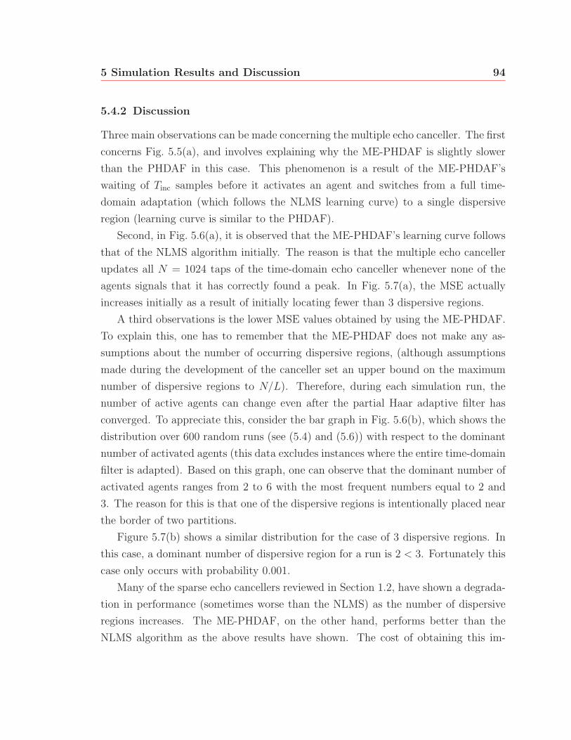
5 Simulation Results and Discussion 94
5.4.2 Discussion
Three main observations can be made concerning the multiple echo canceller. The first
concerns Fig. 5.5(a), and involves explaining why the ME-PHDAF is slightly slower
than the PHDAF in this case. This phenomenon is a result of the ME-PHDAF’s
waiting of Tinc samples before it activates an agent and switches from a full time-
domain adaptation (which follows the NLMS learning curve) to a single dispersive
region (learning curve is similar to the PHDAF).
Second, in Fig. 5.6(a), it is observed that the ME-PHDAF’s learning curve follows
that of the NLMS algorithm initially. The reason is that the multiple echo canceller
updates all N = 1024 taps of the time-domain echo canceller whenever none of the
agents signals that it has correctly found a peak. In Fig. 5.7(a), the MSE actually
increases initially as a result of initially locating fewer than 3 dispersive regions.
A third observations is the lower MSE values obtained by using the ME-PHDAF.
To explain this, one has to remember that the ME-PHDAF does not make any as-
sumptions about the number of occurring dispersive regions, (although assumptions
made during the development of the canceller set an upper bound on the maximum
number of dispersive regions to N/L). Therefore, during each simulation run, the
number of active agents can change even after the partial Haar adaptive filter has
converged. To appreciate this, consider the bar graph in Fig. 5.6(b), which shows the
distribution over 600 random runs (see (5.4) and (5.6)) with respect to the dominant
number of activated agents (this data excludes instances where the entire time-domain
filter is adapted). Based on this graph, one can observe that the dominant number of
activated agents ranges from 2 to 6 with the most frequent numbers equal to 2 and
3. The reason for this is that one of the dispersive regions is intentionally placed near
the border of two partitions.
Figure 5.7(b) shows a similar distribution for the case of 3 dispersive regions. In
this case, a dominant number of dispersive region for a run is 2 < 3. Fortunately this
case only occurs with probability 0.001.
Many of the sparse echo cancellers reviewed in Section 1.2, have shown a degrada-
tion in performance (sometimes worse than the NLMS) as the number of dispersive
regions increases. The ME-PHDAF, on the other hand, performs better than the
NLMS algorithm as the above results have shown. The cost of obtaining this im-
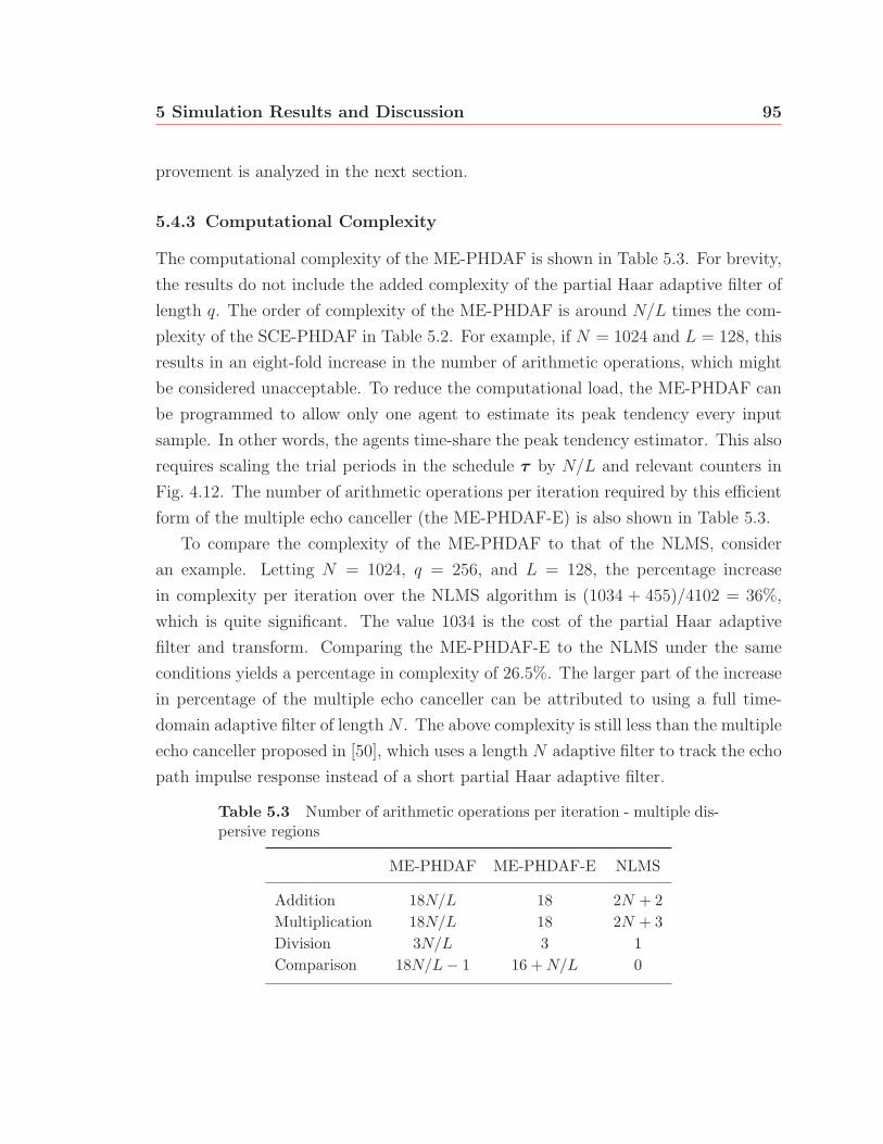
5 Simulation Results and Discussion 95
provement is analyzed in the next section.
5.4.3 Computational Complexity
The computational complexity of the ME-PHDAF is shown in Table 5.3. For brevity,
the results do not include the added complexity of the partial Haar adaptive filter of
length q. The order of complexity of the ME-PHDAF is around N/L times the com-
plexity of the SCE-PHDAF in Table 5.2. For example, if N = 1024 and L = 128, this
results in an eight-fold increase in the number of arithmetic operations, which might
be considered unacceptable. To reduce the computational load, the ME-PHDAF can
be programmed to allow only one agent to estimate its peak tendency every input
sample. In other words, the agents time-share the peak tendency estimator. This also
requires scaling the trial periods in the schedule τ by N/L and relevant counters in
Fig. 4.12. The number of arithmetic operations per iteration required by this efficient
form of the multiple echo canceller (the ME-PHDAF-E) is also shown in Table 5.3.
To compare the complexity of the ME-PHDAF to that of the NLMS, consider
an example. Letting N = 1024, q = 256, and L = 128, the percentage increase
in complexity per iteration over the NLMS algorithm is (1034 + 455)/4102 = 36%,
which is quite significant. The value 1034 is the cost of the partial Haar adaptive
filter and transform. Comparing the ME-PHDAF-E to the NLMS under the same
conditions yields a percentage in complexity of 26.5%. The larger part of the increase
in percentage of the multiple echo canceller can be attributed to using a full time-
domain adaptive filter of lengthN . The above complexity is still less than the multiple
echo canceller proposed in [50], which uses a length N adaptive filter to track the echo
path impulse response instead of a short partial Haar adaptive filter.
Table 5.3 Number of arithmetic operations per iteration - multiple dis-persive regions
ME-PHDAF ME-PHDAF-E NLMS
Addition 18N/L 18 2N + 2Multiplication 18N/L 18 2N + 3Division 3N/L 3 1Comparison 18N/L − 1 16 + N/L 0
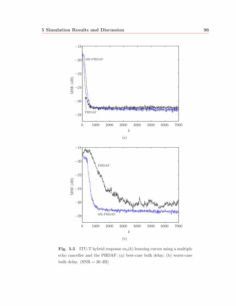
5 Simulation Results and Discussion 96
0 1000 2000 3000 4000 5000 6000 7000
−28
−26
−24
−22
−20
−18
PHDAF
k
MSE
(dB
)
ME-PHDAF
(a)
0 1000 2000 3000 4000 5000 6000 7000
−28
−26
−24
−22
−20
−18
ME-PHDAF
PHDAF
k
MSE
(dB
)
(b)
Fig. 5.5 ITU-T hybrid response m5(k) learning curves using a multiple
echo canceller and the PHDAF: (a) best-case bulk delay; (b) worst-case
bulk delay. (SNR = 30 dB)
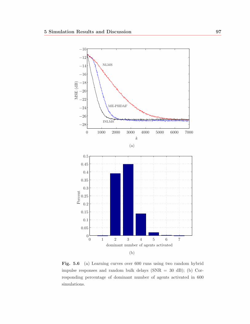
5 Simulation Results and Discussion 97
0 1000 2000 3000 4000 5000 6000 7000
−28
−26
−24
−22
−20
−18
−16
−14
−12
−10
NLMS
ME-PHDAF
INLMS
k
MSE
(dB
)
(a)
00 1 2 3 4 5 6 7
0.05
0.1
0.15
0.2
0.25
0.3
0.35
0.4
0.45
0.5
dominant number of agents activated
Per
cent
(b)
Fig. 5.6 (a) Learning curves over 600 runs using two random hybrid
impulse responses and random bulk delays (SNR = 30 dB); (b) Cor-
responding percentage of dominant number of agents activated in 600
simulations.

5 Simulation Results and Discussion 98
0 1000 2000 3000 4000 5000 6000 7000
−28
−26
−24
−22
−20
−18
−16
−14
−12
−10
−8
NLMS
ME-PHDAF
INLMS
k
MSE
(dB
)
(a)
00 1 2 3 4 5 6 7
0.05
0.1
0.15
0.2
0.25
0.3
0.35
0.4
0.45
0.5
dominant number of agents activated
Per
cent
(b)
Fig. 5.7 (a) Learning curves over 1000 runs using three random hybrid
impulse responses and random bulk delays (SNR = 30 dB); (b) Cor-
responding percentage of dominant number of agents activated in 1000
simulations.
99
Chapter 6
Conclusion
6.1 Thesis Overview and Summary of Results
This thesis has looked at some of the issues of sparse echo cancellation utilizing a
coupled configuration that employs the partial Haar wavelet transform [4]. It began by
analyzing the convergence properties of the coupled configuration, and clarified some
implementation issues which include positioning the short time-domain adaptive, a
partial Haar NLMS algorithm, and the overall complexity of the original coupled echo
canceller [4].
Furthermore, the bulk of this work has presented three major weaknesses of the
coupled echo canceller [4]. First, the partial Haar adaptive filter converges to one
of N/q Wiener solutions with different peak magnitudes, depending on a dispersive
region’s bulk delay. This can seriously hinder the peak delay estimator from correctly
centring the short time-domain adaptive filter around the dispersive region. It was
shown that for small peaks, it takes the peak delay estimator longer to correctly
locate a dispersive region. In pathological cases, the peak delay estimator may take
an extremely large number of input samples to locate a dispersive region. Second, it
was analytically shown that in most instances, the peak delay estimator takes much
longer to track an abrupt change in the echo path impulse response than to initially
locate a peak. Finally, the coupled echo canceller proposed by Bershad and Bist [4]
can not properly cancel multiple echoes.
To support the improvements developed to counter each of these drawbacks, a se-
2006/09/28
6 Conclusion 100
ries of simulation tests were run in MATLAB R©. Different ITU-T G.168 hybrid impulse
responses were used to construct echo path impulse responses to test the proposed
algorithms. These algorithms included the suboptimal context escaping algorithm
(SCE-PHDAF), the improved tracking algorithm (IT-PHDAF), and a multiple echo
cancelling version (ME-PDHAF) of the original coupled echo canceller.
The suboptimal context escape algorithm did not seem to provide dramatic im-
provements in convergence speed in the general case, since the worst-case contexts only
made up a small percentage of the simulation runs. It was shown that for specific
cases, the coupled echo canceller employing suboptimal context escaping was much
faster than the original coupled echo canceller. In addition, the coupled echo canceller
employing suboptimal context escaping was shown to out-perform the original echo
canceller as the SNR dropped from 30 to 10 dB.
The improved tracking algorithm, which includes suboptimal context escaping was
tested under four scenarios of abrupt change in the echo path impulse response. Each
scenario depended on the optimality of the bulk delays (before and after the change)
with respect to the initial context. In all but one scenario, the proposed improved
tracking algorithm was shown to be faster than the original coupled echo canceller
at a small increase in computational complexity (the bulk of this complexity was
attributed to the peak tendency estimator). In these cases, the speed up in tracking
ranged from approximately 500 to 2000 input samples. The case where the proposed
algorithm was shown to be slower was attributed to the waiting time Tinc discussed
in Section 4.4.
The multiple echo canceller was also shown to be sufficiently faster, as compared
to the NLMS algorithm. The multiple echo canceller was first tested on an echo
path impulse response consisting of a single dispersive region. It was shown that for
a worst-case bulk delay, the multiple echo canceller converged much faster than the
original coupled echo canceller [4], while for the best-case bulk delay the proposed
echo canceller was slightly slower due to Tinc. In the case of two and three dispersive
regions, the multiple echo canceller required around 500 input samples to converge to
the same steady-state MSE as an ideal NLMS algorithm, which had prior knowledge
about the locations of the dispersive region. Although much faster than the NLMS
algorithm to reach steady-state, the multiple echo canceller was shown to be costly in
6 Conclusion 101
terms of arithmetic operations. An efficient form was therefore mentioned which can
result in similar performance to the original multiple echo canceller, but at a lower
computational cost.
6.2 Future Work
This thesis has tried to look at adaptive signal processing in a different way, com-
bining belief-based evidence theory with fuzzy inference to incorporate a form of
‘self-awareness’ into an echo canceller. Incorporating forms of expert knowledge can
help devices such as echo cancellers make decisions about their performance in differ-
ent environments. And, if there is support to do so, these devices can then change
the way they function to improve their performance within a specific environment
without the aid of an external operator.
Foreseeable work with regards to the coupled echo canceller in addition to the
proposed algorithms include:
- A more robust approach to decision making in suboptimal-context escaping that
does not rely on a set of trial periods, but on some characteristic of the echo
canceller’s performance. This might require some assumptions about the noise
power, MSE, etc.
- Increasing the flexibility of the multiple echo canceller so that it does not have
to rely on one or more of the assumptions listed in Section 4.5.
- Extending the echo canceller with a subsystem that uses a form of spectral
correlation to determine which subset of partial Haar basis vectors is suitable
for a given echo path impulse response. This is especially important for impulse
responses that are not rich in spectral content [24].
- Analyzing the coupled echo canceller with other classes of adaptive filter algo-
rithms and different combinations thereof for the partial Haar and short time-
domain adaptive filter.
Of course, one of the challenges faced with realizing some of the above proposals will
be keeping the added computational costs as low as possible.
102
References
[1] “Digital network echo cancellers, ITU-T Recommendation G.168,” InternationalTelecommuniation Union, Tech. Rep., Aug. 2004.
[2] P. An, M. Brown, and C. Harris, “On the convergence rate performance of thenormalized least-mean-square adaptation,” IEEE Trans. Neural Networks, vol. 8,pp. 1211–1214, Sept. 1997.
[3] J. Benesty and S. L. Gay, “An improved PNLMS algorithm,” in Proc. IEEE Int.Conf. on Acoustics, Speech, Signal Processing, vol. 2, May 2002, pp. 1881–1884.
[4] N. J. Bershad and A. Bist, “Fast coupled adaptation for sparse impulse responsesusing a partial Haar transform,” IEEE Trans. Signal Processing, vol. 53, no. 3,pp. 966–976, Mar. 2005.
[5] J. R. Boston, “A fuzzy model of signal detection incorporating uncertainty,” inProc. Second IEEE Conf. on Fuzzy Systems, vol. 2, mar 1993, pp. 1107–1112.
[6] ——, “A signal detection system based on Dempster-Shafer theory and compar-ison to fuzzy detection,” Int. Journal Inform. and Security, vol. 9, pp. 13–57,Feb. 2000.
[7] C. Breining, P. Dreiseitel, E. Hansler, A. Mader, B. Nitsch, H. Puder,T. Schertler, G. Schmidt, and H. Tilp, “Acoustic echo control: An application ofvery-high-order adaptive filters,” IEEE Signal Processing Magazine, pp. 42–69,July 1999.
[8] C. S. Burrus, R. A. Gopinath, and H. Guo, Introduction to Wavelets and WaveletTransforms, A Primer, 1st ed. Prentice Hall, Inc., 1998.
[9] J. M. Cioffi and J. A. C. Bingham, “A data-driven multitone echo canceller,”IEEE Trans. Communications, vol. 42, pp. 2853–2869, Oct. 1994.
References 103
[10] C. Cruz, D. A. Pelta, A. S. Royo, and J. L. Verdegay, “Soft computing andcooperative strategies for optimization,” in Proc. IEEE mid-summer Workshopon Soft Computing in Industrial Applications, Espoo, Finland, June 2005.
[11] J. Cui, P. A. Naylor, and D. T. Brown, “An improved IPNLMS algorithm forecho cancellation in packet-switched networks,” in Proc. IEEE Int. Conf. onAcoustics, Speech, Signal Processing, vol. 4, May 2004, pp. 141–144.
[12] H. Deng and M. Doroslovacki, “Improving convergence of the PNLMS algo-rithm for sparse impulse response identification,” IEEE Signal Processing Letters,vol. 12, no. 3, pp. 181–184, Mar. 2005.
[13] J. Dezert, “Foundations for a new theory of plausible and paradoxical reasoning,”Int. Journal Inform. and Security, vol. 9, pp. 13–57, 2002.
[14] J. Dezert, F. Smarandache, and M. Khoshnevisan, “Counter-examples to Demp-ster’s rule of combination,” in Advances and Applications of DSmT for Informa-tion Fusion (Collected Works), J. Dezert and F. Smarandache, Eds. AmericanResearch Press, 2004.
[15] ——, “Presentation of DSmT,” in Advances and Applications of DSmT for Infor-mation Fusion (Collected Works), J. Dezert and F. Smarandache, Eds. AmericanResearch Press, 2004.
[16] D. L. Duttweiler, “Subsampling to estimate delay with application to echo can-celling,” IEEE Trans. Acoustics, Speech, Signal Processing, vol. 31, pp. 1090–1099, Oct. 1983.
[17] ——, “Proportionate normalized least-mean-squares adaptation in echo cancel-ers,” IEEE Trans. Speech and Audio Processing, vol. 8, no. 5, pp. 508–518, Sept.2000.
[18] T. Frantii, “Timing of fuzzy membership functions from data,”Ph.D. dissertation, Oulu University, June 2001. [Online]. Available:http://herkules.oulu.fi/issn03553213/
[19] S. L. Gay, “An efficient, fast converging adaptive filter for network echo cancel-lation,” in Proc. Thirty-Seventh Asilomar Conf. on Signals, Systems, and Com-puters, vol. 1, Nov. 1998, pp. 394–398.
[20] P. H. Giang and P. P. Shenoy, “Statistical decisions using likelihood informationwithout prior probabilities,” in Uncertainty in Artificial Intelligence, A. Darwicheand N. Friedman, Eds. Morgan Kaufmann, San Fransisco, 2002, pp. 170–178.

References 104
[21] A. Graps, “An introduction to wavelets,” IEEE Computational Science and En-gineering, vol. 2, pp. 50–61, 1995.
[22] S. Haykin, Adaptive Filter Theory, 4th ed. Prentice Hall, Inc., 2002.
[23] S. Haykin and B. Widrow, Least-Mean-Square Adaptive Filters. John Wiley andSons Inc., 2003.
[24] K. C. Ho and S. D. Blunt, “Rapid identification of a sparse impulse responseusing an adaptive algorithm in the Haar domain,” IEEE Trans. Signal Processing,vol. 51, no. 3, pp. 628–638, Mar. 2003.
[25] M. Ho, J. M. Cioffi, and J. A. Bingham, “Discrete multitone echo cancelation,”IEEE Trans. Communications, vol. 44, pp. 817–825, July 1996.
[26] J. James, B. Chen, and L. Garrison, “Implementing VoIP: A voice transmissionperformance progress report,” in IEEE Communications Magazine, July 2004,pp. 36–41.
[27] S. Kawamura and M. Hatori, “A tap selection algorithm for adaptive filters,” inProc. IEEE Int. Conf. on Acoustics, Speech, Signal Processing, Apr. 1986, pp.2979–2982.
[28] G. J. Klir and B. Yuan, Fuzzy Sets and Fuzzy Logic: Theory and Applications.Prentice Hall, New Jersey, 1995.
[29] J. Kohlas and P. A. Monney, “Theory of evidence - a survey of its mathemat-ical foundations, applications and computational anaylsis,” ZOR- MathematicalMethods of Operations Research, vol. 39, pp. 35–68, 1994.
[30] J. Liang and T. W. Parks, “A translation-invariant wavelet representation algo-rithm with applications,” IEEE Trans. Signal Processing, vol. 44, pp. 225–232,Feb. 1996.
[31] S. Mallat, A Wavelet Tour of Signal Processing. Academic Press, 1999.
[32] S. G. Mallat, “A theory for multiresolution signal decomposition: the waveletrepresentation,” IEEE Trans. Pattern Analysis and Machine Intelligence, vol. 11,pp. 674–693, July 1989.
[33] R. K. Martin, W. A. Sethares, R. C. Williamson, and C. R. J. Jr., “Exploitingsparsity in adaptive filters,” IEEE Trans. Signal Processing, vol. 50, no. 8, pp.1883–1894, Aug. 2002.
References 105
[34] H. McKinlay, “A legacy of echo and silence,” in Telecomm. Quality of Services:The Business of Success, QoS 2004, IEE, Mar. 2004, pp. 109–113.
[35] J. M. Mendel, “Fuzzy logic systems for engineering,” Proc. of the IEEE, vol. 83,no. 3, pp. 345–377, Mar. 1995.
[36] A. Papoulis and S. U. Pillai, Probability, Random Variables and Stochastic Pro-cesses, 4th ed. McGraw-Hill Science/Engineering/Math, 2001.
[37] J. Pearl, Probabilistic Reasoning in Intelligent Systems: Networks of PlausibleInference. Morgan Kaufmann Publishers, 1988.
[38] K. Sayood, Introduction to Data Compression, 2nd ed. Morgan KaufmannPublishers, 2000.
[39] I. W. Selesnick, “Hilbert transform pairs of wavelet bases,” IEEE Signal Process-ing Letters, vol. 8, pp. 170–173, June 2001.
[40] ——, “The design of approximate hilbert transform pairs of wavelet bases,” IEEETrans. Signal Processing, vol. 50, pp. 1144–1152, May 2002.
[41] K. Shenoi, Digital Signal Processing in Telecommunications. Prentice Hall, Inc.,1995.
[42] M. J. Shensa, “The discrete wavelet transform: Wedding the a Trous and Mallatalgorithms,” IEEE Trans. Signal Processing, vol. 40, pp. 2464–2482, Oct. 1992.
[43] E. P. Simoncelli, W. T. Freeman, E. H. Adelson, and D. J. Heeger, “Shiftablemultiscale transforms,” IEEE Trans. Inform. Theory, vol. 38, pp. 587–607, Mar.1992.
[44] P. Smets, “Decision making in the TBM: the necessity of the pignistic trans-formation,” Int. Journal of Approximate Reasoning, vol. 38, pp. 133–147, Feb.2005.
[45] P. Smets and R. Kennes, “The transferable belief model,” Artificial Intelligence,vol. 66, no. 2, pp. 191–234, Apr. 1994.
[46] A. Sugiyama and S. Ikeda, “A fast convergence algorithm for adaptive FIR filterswith sparse taps,” IEICE Trans. Fundamentals, vol. E77-A, pp. 681–686, Apr.1994.

References 106
[47] A. Tchamova, T. Semerdjiev, and J. Dezert, “Estimation of target behavior ten-dencies using DSmT,” in Advances and Applications of DSmT for InformationFusion (Collected Works), J. Dezert and F. Smarandache, Eds. American Re-search Press, 2004.
[48] S. V. Vaseghi, Advanced Signal Processing and Digital Noise Reduction. JohnWiley and Sons Ltd. and B.G. Teubner, 1996.
[49] R. R. Yager and D. P. Filev, Essentials of Fuzzy Modeling and Control. JohnWiley and Sons, Inc., 1994.
[50] P. C.-W. Yip and D. M. Etter, “An adaptive multiple echo canceller for slowlytime-varying echo paths,” IEEE Trans. Communications, vol. 38, pp. 1693–1698,Oct. 1990.
[51] L. A. Zadeh, “The role of fuzzy logic in the management of uncertainty in expertsystems,” Fuzzy Sets and Systems, vol. 11, no. 1, pp. 199–227, 1999.


![Hand Gesture Recognition Using Haar-Like Features and ... · Haar-like feature which was proposed by Lienhart and Maydt [5]. The value of a Haar-like feature is difference between](https://img.pdfslide.us/doc/110x75/5e159b2789c350181e471154/hand-gesture-recognition-using-haar-like-features-and-haar-like-feature-which.jpg)