Eotvos Lorand University

Faculty of Science

Donat NagyMathemathics MSc

Haar null and Haar meager setsSmall sets in non-locally-compact Polish groups

Master’s thesis

Supervisor: Marton Elekes

Department of Analysis

Budapest, 2016.

Acknowledgements

I would like to thank my supervisor, Marton Elekes, for introducing me to this

subject and for his suggestions and corrections during the preparation of the present

work. The inspiration provided by his enthusiasm was and will be invaluable for my

studies and research.

3

Contents

1 Introduction and history 5

2 Notation and terminology 8

3 Basic properties 10

3.1 Core definitions . . . . . . . . . . . . . . . . . . . . . . . . . . . . . . 10

3.2 Notions of smallness . . . . . . . . . . . . . . . . . . . . . . . . . . . 11

3.3 Connections to Haar measure and meagerness . . . . . . . . . . . . . 15

4 Alternative definitions 21

4.1 Equivalent versions . . . . . . . . . . . . . . . . . . . . . . . . . . . . 21

4.2 Coanalytic hulls . . . . . . . . . . . . . . . . . . . . . . . . . . . . . . 28

4.3 Naive versions . . . . . . . . . . . . . . . . . . . . . . . . . . . . . . . 28

4.4 Left and right Haar null sets . . . . . . . . . . . . . . . . . . . . . . . 30

4.5 Openly Haar null sets . . . . . . . . . . . . . . . . . . . . . . . . . . . 34

4.6 Strongly Haar meager sets . . . . . . . . . . . . . . . . . . . . . . . . 37

5 Analogs of the results from the locally compact case 39

5.1 Fubini’s theorem and the Kuratowski-Ulam theorem . . . . . . . . . . 39

5.2 The Steinhaus theorem . . . . . . . . . . . . . . . . . . . . . . . . . . 45

5.3 The countable chain condition . . . . . . . . . . . . . . . . . . . . . . 49

6 Common techniques 51

6.1 Probes . . . . . . . . . . . . . . . . . . . . . . . . . . . . . . . . . . . 51

6.2 Application of the Steinhaus theorem . . . . . . . . . . . . . . . . . . 52

6.3 Compact sets are small . . . . . . . . . . . . . . . . . . . . . . . . . . 53

6.4 Random construction . . . . . . . . . . . . . . . . . . . . . . . . . . . 56

6.5 Sets containing translates of all compact sets . . . . . . . . . . . . . . 57

References 59

4

1 Introduction and history

Many results in various branches of mathematics state that certain properties hold

for almost every element of a space. In the continuous, large structures which are

frequently studied in analysis it is common to encounter a property that is true for

most points, but false on a negligibly small part of the structure. For example, for a

Lebesgue measurable set A ⊆ Rn the set of points where the density of A is neither

0 nor 1 always has Lebesgue measure zero by Lebesgue’s density theorem, but it is

known that there are always such exceptional points, unless either A or Rn \ A has

measure zero. These situations mean that there are facts which can be grasped only

by defining a suitable notion of smallness and stating that the exceptional elements

form a small set.

In the Euclidean space Rn there is a generally accepted, natural notion of small-

ness: a set is considered to be small if it has Lebesgue measure zero. As this notion

is defined by a measure, which is by definition countably additive, these small sets

are closed under countable unions and hence form a σ-ideal. The Lebesgue measure

is essentially defined by the fact that it is translation invariant (and satisfies some

technical properties). This allows us to generalize it to topological groups (we need

a group structure for the translations and a topological structure for the technical

properties).

This generalized notion (which was introduced by Alfred Haar in 1933) is called

the Haar measure (when the group is not commutative, either left multiplication or

right multiplication can be the generalized notion corresponding to translation and

hence we get left and right Haar measures). (We summarize the definition and the

basic properties of the Haar measures in subsection 3.3, a deeper analysis can be

found e.g. in [13, §15].) It is possible to show that (e.g. left) Haar measures exist

on a topological group if and only if it is locally compact, and in locally compact

groups the left Haar measures are unique up to multiplication by a constant (see

Theorem 3.3.3 and Theorem 3.3.11). This means that in locally compact groups one

can define a natural notion of smallness by saying that a set is small if it has (e.g.

left) Haar measure zero, but this method says nothing about non-locally-compact

groups.

In the paper [3] (which was published in 1972) Christensen introduced Haar null

sets, which are defined in all abelian Polish groups and coincide with the sets of Haar

measure zero in the locally compact case. Twenty years later Hunt, Sauer and Yorke

independently introduced this notion under the name of shy sets in the paper [15].

Since then lots of papers were published which either study some property of Haar

null sets or use this notion of smallness to state facts which are true for almost every

element of some structure. It was relatively easy to generalize this notion to non-

abelian groups, on the other hand, the assumption that the topology is Polish (that

5

is, separable and completely metrizable) is still almost always assumed, because it

turned out to be convenient and useful.

Haar null sets are translation invariant in the strong sense that if X is Haar

null, then gXh = {gxh : x ∈ X} is Haar null for every pair of elements g, h from

the group. The definition of Haar null sets is chosen in a way that makes this fact

trivial: a (Borel) set is Haar null if there is a (Borel probability) measure that assigns

measure zero to every such translate of a set. It is possible to prove that Haar null

sets form a σ-ideal (see Theorem 3.2.5).

There is another widely used notion of smallness, the notion of meager sets (also

known as sets of the first category). Meager sets can be defined in any topological

space; a set is said to be meager if it is the countable union of nowhere dense sets.

It is trivial that meager sets form a σ-ideal, and it is also clear that this notion

is translation invariant in topological groups. A topological space is called a Baire

space if the nonempty open sets are non-meager; this basically means that one can

consider the meager sets small in these spaces. The Baire category theorem states

that all completely metrizable spaces and all locally compact Hausdorff spaces are

Baire spaces (see [17, Theorem 8.4] for the proofs).

In locally compact groups the system of meager sets and the system of sets of

Haar measure zero share many properties; for example the classical Erdos-Sierpinski

duality theorem states that it is consistent that there is a bijection f : R→ R such

that f(A) is meager if and only if A ⊆ R has Lebesgue measure zero and f(A) has

Lebesgue measure zero if and only if A ⊆ R is meager. Despite this, there are sets

that are small in one sense and far from being small in the other sense, for example

every abelian locally compact group can be written as the union of a meager set and

a set of Haar measure zero.

In 2013, Darji defined the notion of Haar meager sets in the paper [5] to provide a

better analog of Haar null sets in the non-locally-compact case. Darji only considered

abelian Polish groups, but [7] generalized this notion to non-abelian Polish groups.

Haar meager sets coincide with meager sets in locally compact Polish groups, and

Haar meagerness is a strictly weaker notion than meagerness in non-locally-compact

abelian groups (see Theorem 3.3.13 and Theorem 3.3.14). The difference between

the definition of Haar null and Haar meager sets is that for Haar meager sets we

require the existence of a continuous map from a compact metric space to the group

that assigns meager preimages to the translates of our set (instead of the existence

of a measure that assigns measure zero to the translates). The analogy between the

definitions mean that most of the results for Haar null sets are also true for Haar

meager sets and often can be proved using similar methods.

The goal of this thesis is to introduce these two notions and collect those basic

results about them that are useful for proving new results. Of course the boundary

between applicable and not applicable results is blurry, but we tried to include

6

the most frequently used lemmas and the counterexamples showing that some usual

property cannot be generalized and must be avoided in the proofs. This focus means

that we do not include the applications of this theory in concrete cases except as

illustrations for proof techniques. The majority of the results are included with

proofs to illustrate the ideas and methods of this area, but especially in the later

sections we frequently omit proofs that are too technical, only distantly related to

this area or simply too long.

At the beginning, in section 2, we introduce the notions, definitions and conven-

tions which are not related to our area, but used repeatedly in this thesis. Then

section 3 defines the core notions and investigates their most important properties.

After these, section 4 considers the modified variants of the definitions. This

section starts with a large collection of equivalent definitions for our core notions,

then lists and briefly describes most of the versions which appear in the literature

and are not (yet proved to be) equivalent to the “plain” versions.

The next section, section 5, considers the feasibility of generalizing three well-

known results (Fubini’s theorem, the Steinhaus theorem and the countable chain

condition) for non-locally-compact Polish groups. Unfortunately, most of the an-

swers are given in form of counterexamples, but weakened variants of the first two

results can be salvaged and these are useful as lemmas.

Finally, in section 6 we discuss some proof techniques for questions from this

area. Some of these are essentially useful lemmas, the others are just ideas and ways

of thinking which can be helpful in certain cases.

7

2 Notation and terminology

This section is the collection of the miscellaneous notations, definitions and conven-

tions that are used repeatedly in this thesis.

The symbols N and ω both refer to the set of nonnegative integers. We write Nif we consider this set as a topological space (with the discrete topology) and ω if

we use it only as a cardinal, ordinal or index set. (For example we write the Polish

space of the countably infinite sequences of natural numbers as Nω.) We consider

the nonnegative integers as von Neumann ordinals, i.e. we identify the nonnegative

integer n with the set {0, 1, 2, . . . , n− 1}.

P(S) denotes the power set of a set S. For a set S ⊆ X×Y , x ∈ X and y ∈ Y , Sxis the x-section Sx = {y : (x, y) ∈ S} and Sy is the y-section Sy = {x : (x, y) ∈ S}.

If S is a subset of a topological space, int(S) is the interior of S and S is the

closure of S. We consider N, Z and all finite sets to be topological spaces with the

discrete topology. (Note that this convention allows us to simply write the Cantor

set as 2ω(= {0, 1}ω).) If X is a topological space, then

B(X) denotes its Borel subsets (B(X) is the σ-algebra generated by the open sets,

see [17, Chapter II]),

M(X) denotes its meager subsets (a set is meager if it is the union of countably

many nowhere dense sets and a set is nowhere dense if the interior of its

closure is empty, see [17, §8.A]).

If the space X is Polish (that is, separable and completely metrizable), then

Σ11(X) denotes its analytic subsets (a set is analytic if it is the continuous image of

a Borel set, see [17, Chapter III]),

Π11(X) denotes its coanalytic subsets (a set is coanalytic if its complement is ana-

lytic, see [17, Chapter IV]).

If the topological space X is clear from the context, we simply write B,M, Σ11 and

Π11.

In a metric space (X, d), diam(S) = sup{d(x, y) : x, y ∈ S} denotes the diameter

of the subset S. If x ∈ X and r > 0, then B(x, r) = {x′ ∈ X : d(x, x′) < r} and

B(x, r) = {x′ ∈ X : d(x, x′) ≤ r} denotes respectively the open and the closed ball

ball with center x and radius r in X.

If µ is an outer measure on a set X, we say that A ⊆ X is µ-measurable if

µ(B) = µ(B ∩A) + µ(B \A) for every B ⊆ X. Unless otherwise stated, we identify

an outer measure µ with its restriction to the µ-measurable sets and “measure”

means an outer measure or the complete measure that is identified by it this way.

A measure µ is said to be Borel if all Borel sets are µ-measurable. The support of

the measure µ is denoted by suppµ.

8

Almost all of our results will be about topological groups. A set G is called a

topological group if is equipped with both a group structure and a Hausdorff topology

and these structures are compatible, that is, the multiplication map G × G → G,

(g, h) 7→ gh and the inversion map G → G, g 7→ g−1 are continuous functions. We

make the convention that whenever we require a group to have some topological

property (for example a “compact group”, a “Polish group”, . . . ), then it means that

the group must be a topological group and have that property (as a topological

space). The identity element of a group G will be denoted by 1G.

Most of the results in this thesis are about certain subsets of Polish groups.

Unless otherwise noted, (G, ·) denotes an arbitrary Polish group. We denote the

group operation by multiplication even when we assume that the (abstract) group

under consideration is abelian, but we write the group operation of well-known

concrete abelian groups like (R,+) or (Zω,+) as addition.

Some techniques only work in Polish groups that admit a two-sided invariant

metric. (A metric d on G is called two-sided invariant (or simply invariant) if

d(g1hg2, g1kg2) = d(h, k) for any g1, g2, h, k ∈ G.) Groups with this property are

also called TSI groups. This class of groups properly contains all Polish, abelian

groups, since each metric group G admits a left-invariant metric which, obviously, is

invariant when G is abelian. Any invariant metric on a Polish group is automatically

complete. For proofs of these facts and more results about TSI groups see for

example [13, §8.].

Some basic results can be generalized for non-separable groups, but we will only

deal with the separable case. On the other hand, many papers about this topic only

consider abelian groups or some class of vector spaces. When the proof of a positive

result can be generalized for arbitrary Polish group, we will usually do so, but we will

usually provide counterexamples only in the special case where their construction is

the simplest. If we assume that G is locally compact, our notions will coincide with

simpler notions (see subsection 3.3) and the majority of the results in this thesis

become significantly easier to prove, so the interesting case is when G is not locally

compact.

9

3 Basic properties

3.1 Core definitions

This subsection introduces the core notions of this thesis. Both notions have sev-

eral slightly different formalizations in the literature. The terminology used in this

thesis is based on the terminology of [8]. The various equivalent forms of these defi-

nitions and some variants which are similar, but lack some important properties are

discussed in section 4.

Haar null sets were first introduced by Christensen in [3] in 1972 as a general-

ization of the null sets of the Haar measure. (The Haar measure itself cannot be

generalized for groups that are non-locally-compact, see Theorem 3.3.11.) Twenty

years later in [15] Hunt, Sauer and Yorke independently introduced Haar null sets

under the name “shy sets”.

Definition 3.1.1. A set A ⊆ G is said to be Haar null if there are a Borel set

B ⊇ A and a Borel probability measure µ on G such that µ(gBh) = 0 for every

g, h ∈ G. A measure µ satisfying this is called a witness measure for A. The system

of Haar null subsets of G is denoted by HN = HN (G).

Remark 3.1.2. Using the terminology introduced in [15], a set A ⊆ G is called shy

if it is Haar null, and prevalent if G \ A is Haar null.

Some authors (including Christensen) write “universally measurable set” instead

of “Borel set” when they define Haar null sets. This version is not equivalent to

the original, but most results can be proved for both notions in the same way.

When a paper uses both notions, sets satisfying this alternative definition are called

“generalized Haar null sets”.

Definition 3.1.3. If X is a Polish space, a set A ⊆ X is called universally measur-

able if it is µ-measurable for any σ-finite Borel measure µ on X.

Definition 3.1.4. A set A ⊆ G is said to be a generalized Haar null if there are

a universally measurable set B ⊇ A and a Borel probability measure µ on G such

that µ(gBh) = 0 for every g, h ∈ G. A measure µ satisfying this is called a witness

measure for A. The system of generalized Haar null subsets of G is denoted by

GHN = GHN (G)

Remark 3.1.5. As every Borel set is universally measurable, every Haar null set is

generalized Haar null.

Haar meager sets were first introduced by Darji in [5] in 2013 as a topological

counterpart to the Haar null sets. (Meagerness remains meaningful in non-locally-

compact groups, but Haar meager sets are a better analogue for Haar null sets.)

10

Definition 3.1.6. A set A ⊆ G is said to be Haar meager if there are a Borel set

B ⊇ A, a (nonempty) compact metric space K and a continuous function f : K → G

such that f−1(gBh) is meager in K for every g, h ∈ G. A function f satisfying this is

called a witness function for A. The system of Haar meager subsets of G is denoted

by HM = HM(G).

3.2 Notions of smallness

Both “Haar null” and “Haar meager” are notions of smallness (i.e. we usually think

of Haar null and Haar meager sets as small or negligible). This point of view is

justified by the fact that both the system of Haar null sets and the system of Haar

meager sets are σ-ideals.

Definition 3.2.1. A system I (of subsets of some set) is called a σ-ideal if

(I) ∅ ∈ I,

(II) A ∈ I, B ⊆ A⇒ B ∈ I and

(III) if An ∈ I for all n ∈ ω, then⋃nAn ∈ I.

To prove that these systems are indeed σ-ideals we will need some technical

lemmas.

Lemma 3.2.2. If µ is a Borel probability measure on G and U is a neighborhood of

1G, then there are a compact set C ⊆ G and c ∈ G with µ(C) > 0 and C ⊆ cU .

Proof. Applying [17, Theorem 17.11], there exists a compact set C ⊆ X with µ(C) ≥12. Fix an open set V with 1G ∈ V ⊂ V ⊂ U . The collection of open sets {cV : k ∈C} covers C and C is compact, so C =

⋃c∈F (cV ∩C) for some finite set F ⊆ C. It is

clear that µ(cV ∩ C) must be positive for at least one c ∈ F . Choosing C = cV ∩ Cclearly satisfies our requirements.

Corollary 3.2.3. If µ is a Borel probability measure on G, U is a neighborhood of

1G, B ⊆ G is universally measurable and satisfies µ(gBh) = 0 for every g, h ∈ G,

then there exists a Borel probability measure µ′ that satisfies µ′(gBh) = 0 for every

g, h ∈ G and has a compact support that is contained in U .

Proof. It is easy to check that µ′(X) := µ(cX∩C)µ(C)

satisfies our requirements.

Lemma 3.2.4. Let d be a metric on G that is compatible with the topology of G. If

L ⊆ G is compact and ε > 0 is arbitrary, then there exists a neighborhood U of 1Gsuch that d(x · u, x) < ε for every x ∈ L and u ∈ U .

11

Proof. (Reproduced from [7, Lemma 2].) By the continuity of the function (x, u) 7→d(x · u, x), for every x ∈ L there are neighborhoods Vx of x and Ux of 1G such that

the image of Vx × Ux is a subset of [0, ε). Let F ⊆ L be a finite set such that

L ⊆⋃x∈F Vx. It is easy to check that U =

⋂x∈F Ux satisfies our conditions.

Theorem 3.2.5.

(1) The system HN of Haar null sets is a σ-ideal.

(2) The system GHN of generalized Haar null sets is a σ-ideal.

Proof. It is trivial that both HN and GHN satisfy (I) and (II) in Definition 3.2.1.

The proof of (III) that is reproduced in this thesis is from the appendix of [4], where

a corrected version of the proof in [20] is given. Proving this fact is easier in abelian

Polish groups (see [3, Theorem 1]) and when the group is metrizable with a complete

left invariant metric (this would allow the proof of [20, Theorem 3] to work without

modifications). The appendix of [4] mentions the other approaches and discusses

the differences between them.

The proof of (III) for Haar null and for generalized Haar null sets is very similar.

The following proof will be for Haar null sets, but if “Borel set” is replaced with

“universally measurable set”and“Haar null” is replaced with“generalized Haar null”,

it becomes the proof for generalized Haar null sets.

Let An be Haar null for all n ∈ ω. By definition there are Borel sets Bn ⊆ G and

Borel probability measures µn on G such that An ⊆ Bn and µn(gBnh) = 0 for every

g, h ∈ G. Let d be a complete metric on G that is compatible with the topology of

G (as G is Polish, it is completely metrizable).

We construct for all n ∈ ω a compact set Cn ⊆ G and a Borel probability measure

µn such that the support of µn is Cn, µn(gBnh) = 0 for every g, h ∈ G (i.e. µn is a

witness measure) and the “size” of the sets Cn decreases “quickly”.

The construction will be recursive. For the initial step use Corollary 3.2.3 to find

a Borel probability measure µ0 that satisfies µ0(gB0h) = 0 for every g, h ∈ G and

that has compact support C0 ⊆ G. Assume that µn′ and Cn′ are already defined

for all n′ < n. By Lemma 3.2.4 there exists a neighborhood Un of 1G such that

if u ∈ Un, then d(k · u, k) < 2−n for every k in the compact set C0C1C2 · · ·Cn−1.

Applying Corollary 3.2.3 again we can find a Borel probability measure µn that

satisfies µn(gBnh) = 0 for every g, h ∈ G and that has a compact support Cn ⊆ Un.

If cn ∈ Cn for all n ∈ ω, then it is clear that the sequence (c0c1c2 · · · cn)n∈ωis a Cauchy sequence. As (G, d) is complete, this Cauchy sequence is convergent;

we write its limit as the infinite product c0c1c2 · · · . The map ϕ :∏

n∈ω Cn → G,

ϕ((c0, c1, c2, . . .)) = c0c1c2 · · · is the uniform limit of continuous functions, hence it

is continuous.

12

Let µΠ be the product of the measures µn on the product space CΠ :=∏

n∈ω Cn.

Let µ = ϕ∗(µΠ) be the push-forward of µΠ along ϕ onto G, i.e.

µ(X) = µΠ(ϕ−1(X)) = µΠ({

(c0, c1, c2, . . .) ∈ CΠ : c0c1c2 · · · ∈ X}).

We claim that µ witnesses that A =⋃n∈ω An is Haar null. Note that A is

contained in the Borel set B =⋃n∈ω Bn, so it is enough to show that µ(gBh) = 0

for every g, h ∈ G. As µ is σ-additive, it is enough to show that µ(gBnh) = 0 for

every g, h ∈ G and n ∈ ω.

Fix g, h ∈ G and n ∈ ω. Notice that if cj ∈ Cj for every j 6= n, j ∈ ω, then

µn ({cn ∈ Cn : c0c1c2 · · · cn · · · ∈ gBnh}) =

= µn((c0c1 · · · cn−1)−1 · gBnh · (cn+1cn+2 · · · )−1) = 0

because µn(g′Bnh′) = 0 for all g′, h′ ∈ G. Applying Fubini’s theorem in the product

space(∏

j 6=nCj

)× Cn to the product measure

(∏j 6=n µj

)× µn yields that

0 = µΠ({

(c0, c1, . . . , cn, . . .) ∈ CΠ : c0c1 · · · cn · · · ∈ gBnh}).

By the definition of µ this means that µ(gBnh) = 0.

Theorem 3.2.6. The system HM of Haar meager sets is a σ-ideal.

Proof. The proof of (I) and (II) in Definition 3.2.1 is trivial again. The proof of (III)

is reproduced from [7, Theorem 3]. This proof will be very similar to the proof of

Theorem 3.2.5, but restricting the witnesses to a smaller “part” of G is simpler in

this case (we do not need an analogue of Corollary 3.2.3).

Let An be Haar meager for all n ∈ ω. By definition there are Borel sets Bn ⊆ G,

compact metric spaces Kn 6= ∅ and continuous functions fn : Kn → G such that

f−1n (gBnh) is meager in Kn for every g, h ∈ G. Let d be a complete metric on G

that is compatible with the topology of G.

We construct for all n ∈ ω a compact metric space Kn and a continuous function

fn : Kn → G satisfying that f−1n (gBnh) is meager in Kn for every g, h ∈ G (i.e. fn

is a witness function) and the “size” of the images fn(Kn) ⊆ G decreases “quickly”.

Unlike the Haar null case, we do not have to apply recursion in this construction.

By Lemma 3.2.4 there exists a neighborhood Un of 1G such that if u ∈ Un, then

d(k · u, k) < 2−n for every k in the compact set f0(K0)f1(K1) · · · fn−1(Kn−1). Let

xn ∈ fn(Kn) be an arbitrary element and Kn = f−1n (xnUn). The set Kn is compact

(because it is a closed subset of a compact set) and nonempty. Let fn : Kn → G,

fn(k) = x−1n fn(k), this is clearly continuous.

Claim 3.2.7. For every n ∈ ω and g, h ∈ G, f−1n (gBnh) is meager in Kn.

13

Proof. Fix n ∈ ω and g, h ∈ G. The set f−1n (Un) is open in Kn and because f is a

witness function, the set f−1n (gBnh) = f−1

n (xngBnh) is meager in Kn. This means

that f−1n (Un) ∩ f−1

n (gBnh) is meager in f−1n (Un). Since each open subset of Kn is

comeager in its closure and the closure of f−1n (Un) = f−1

n (xnUn) is f−1n (xnUn) = Kn,

simple formal calculations yield that f−1n (gBnh) ∩ Kn is meager in Kn.

Let K be the compact set∏

n∈ω Kn and for n ∈ ω let ψn be the continuous

function ψn : K → G,

ψn(k) = f0(k0) · f1(k1) · . . . · fn−1(kn−1).

By the choice of Un we obtain d(ψn−1(k), ψn(k)) ≤ 2−n for every k ∈ K. Using the

completeness of d this means that the sequence of functions (ψn)n∈ω is uniformly

convergent. Let f : K → G be the limit of this sequence. f is continuous, because

it is the uniform limit of continuous functions.

We claim that f witnesses that A =⋃n∈ω An is Haar meager. Note that A is

contained in the Borel set B =⋃n∈ω Bn, so it is enough to show that f−1(gBh) is

meager in K for every g, h ∈ G. As meager subsets of K form a σ-ideal, it is enough

to show that f−1(gBnh) is meager in K for every g, h ∈ G and n ∈ ω.

Fix g, h ∈ G and n ∈ ω. Notice that if kj ∈ Kj for every j 6= n, j ∈ ω, then

Claim 3.2.7 means that

{kn ∈ Kn : f(k0, k1, . . . , kn, . . .) ∈ gBnh} =

= {kn ∈ Kn : f0(k0) · f1(k1) · . . . · fn(kn) · . . . ∈ gBnh}

= f−1n

((f0(k0) · . . . fn−1(kn−1)

)−1

· gBnh ·(fn+1(kn+1) · fn+2(kn+2) · . . .

)−1)

is meager in Kn. Applying the Kuratowski-Ulam theorem (see e.g. [17, Theorem

8.41]) in the product space(∏

j 6=n Kj

)×Kn, the Borel set f−1(gBnh) is meager.

As the group G acts on itself via multiplication, it is useful if this action does not

convert “small” sets into “large” ones. This means that a “nice” notion of smallness

must be a translation invariant system.

Definition 3.2.8. A I ⊆ P(G) system is called translation invariant if A ∈ I ⇔gAh ∈ I for every A ⊆ G and g, h ∈ G.

Proposition 3.2.9. The σ-ideals HN , GHN and HM are all translation invariant.

Proof. This is clear from Definition 3.1.1, Definition 3.1.4 and Definition 3.1.6.

14

If a nontrivial notion of smallness has these “nice” properties, then the following

lemma states that countable sets are small and nonempty open sets are not small.

Applying this simple fact for our σ-ideals is often useful in simple cases.

Lemma 3.2.10. Let I be a translation invariant σ-ideal that contains a nonempty

set but does not contain all subsets of G. If A ⊆ G is countable, then A ∈ I, and if

U ⊆ G is nonempty open, then U /∈ I.

Proof. If x ∈ G, then any nonempty set in I has a translate that contains {x}as a subset, hence {x} ∈ I. Using that I is closed under countable unions, this

yields that if A ⊆ G is countable, then A ∈ I. To prove the other claim, suppose

for a contradiction that U ⊆ G is a nonempty open set that is in I. It is clear

that G =⋃g∈G gU , and as G is Lindelof, G =

⋃n∈ω gnU for some countable subset

{gn : n ∈ ω} ⊆ G. But here gnU ∈ I (because I is translation invariant) and thus

G ∈ I (because I is closed under countable unions), and this means that I contains

all subsets of G, and this is a contradiction.

Remark 3.2.11. Let I be one of the σ-ideals HN , GHN and HM. If G is count-

able, then I = {∅}, otherwise I contains a nonempty set and does not contain all

subsets of G.

3.3 Connections to Haar measure and meagerness

This section discusses the connection between sets with Haar measure zero and

Haar null sets and the connection between meager sets and Haar meager sets. In

the simple case when G is locally compact we will find that equivalence holds for

both pairs, justifying the names “Haar null” and “Haar meager”. When G is non-

locally-compact, we will see that the first connection is broken by the fact that there

is no Haar measure on the group. For the other pair we will see that Haar meager

sets are always meager, but there are Polish groups where the converse is not true.

First we recall some well-known facts about Haar measures. For proofs and more

detailed discussion see for example [13, §15].

Definition 3.3.1. If (X,Σ) is a measurable space with B(X) ⊆ Σ, then a measure

µ : Σ → [0,∞] is called regular if µ(U) = sup{µ(K) : K ⊆ U,K is compact} for

every U open set and µ(A) = inf{µ(U) : A ⊆ U,U is open} for every set A in the

domain of µ.

Definition 3.3.2. If G is a topological group (not necessarily Polish), a measure

λ : B(G)→ [0,∞] is called a left Haar measure if it satisfies the following properties:

(I) λ(F ) <∞ if F is compact,

(II) λ(U) > 0 if U is a nonempty open set,

15

(III) λ(gB) = λ(B) for all B ∈ B(G) and g ∈ G (left invariance),

(IV) λ is regular.

If left invariance is replaced by the property λ(Bg) = λ(B) for all B ∈ B(G) and

g ∈ G (right invariance), the measure is called a right Haar measure.

Theorem 3.3.3. (existence of the Haar measure) If G is a locally compact group

(not necessarily Polish), then there exists a left (right) Haar measure on G and if

λ1, λ2 are two left (right) Haar measures, then λ1 = c ·λ2 for a positive real constant

c.

If G is compact, (I) means that the left and right Haar measures are finite

measures, and this fact can be used to prove the following result:

Theorem 3.3.4. If G is a compact group, then all left Haar measures are right

Haar measures and vice versa.

This result is also trivially true in abelian locally compact groups, but not true

in all locally compact groups. However, the following result remains true:

Theorem 3.3.5. If G is a locally compact group, then the left Haar measures and

the right Haar measures are absolutely continuous relatively to each other, that is,

for every Borel set B ⊆ G, either every left Haar measure and every right Haar

measure assigns measure zero to B or no left Haar measure and no right Haar

measure assigns measure zero to B.

This allows us to define the following notion:

Definition 3.3.6. Suppose that G is a locally compact group and fix an arbitrary

left (or right) Haar measure λ. We say that a set N ⊆ G has Haar measure zero if

N ⊆ B for some Borel set B with λ(B) = 0. The collection of these sets is denoted

by N = N (G).

Definition 3.3.2 defines the Haar measures only on the Borel sets. If λ is an arbi-

trary left (or right) Haar measure, we can complete it using the standard techniques.

The domain of the completion will be σ(B(G) ∪N ) (the σ-algebra generated by Nand the Borel sets). For every set A in this σ-algebra, let

λ(A) = sup

{∑j∈ω

λ(Bj) : Bj ∈ B(G), A ⊆⋃j∈ω

(Bj)

}.

This completion will be a complete measure that agrees with the original λ on Borel

sets and satisfies properties (I) – (IV) from Definition 3.3.2 (or right invariance

instead of left invariance if λ was a right Haar measure). We will identify a left (or

right) Haar measure with its completion and we will also call this extension (slightly

imprecisely) a left (or right) Haar measure.

16

Theorem 3.3.7. If G is a locally compact Polish group, then system of sets with

Haar measure zero is the same as the system of Haar null sets and is the same as

the system of generalized Haar null sets, that is, N (G) = HN (G) = GHN (G).

Proof. N (G) ⊆ HN (G):

Let λ be a left Haar measure and λ′ be a right Haar measure. If N ∈ N (G) is

arbitrary, then by definition there is a Borel set B satisfying N ⊆ B and λ(B) =

0. The left invariance of G means that λ(gB) = 0 for every g ∈ G. Applying

Theorem 3.3.5 this means that λ′(gB) = 0 for every g ∈ G, and applying the right

invariance of λ′ we get that λ′(gBh) = 0 for every g, h ∈ G. Using the regularity of

λ′, it is easy to see that there is a compact set K with 0 < λ′(K) <∞. The measure

µ(X) = λ′(K∩X)λ′(K)

is clearly a Borel probability measure. µ� λ′ means that µ(gBh) =

0 for every g, h ∈ G, so B and µ satisfy the requirements of Definition 3.1.1.

HN (G) ⊆ GHN (G):

This is trivial in all Polish groups, see Remark 3.1.5.

GHN (G) ⊆ N (G):

Suppose that A ∈ GHN (G). By definition there exists an universally measurable

B ⊆ G and a Borel probability measure µ such that µ(gBh) = 0 for every g, h ∈ G.

Notice that we will only use that µ(Bh) = 0 for every h ∈ G, so we will also

prove that (using the terminology of subsection 4.4) all generalized right Haar null

sets have Haar measure zero. Let λ be a left Haar measure on G. Let m be the

multiplication map m : G×G→ G, (x, y) 7→ x · y.

Notice that the set m−1(B) = {(x, y) ∈ G × G : x · y ∈ B} is universally

measurable in G × G, because it is the preimage of a universally measurable set

under the continuous map m. (This follows from that that the preimage of a Borel

set under m is Borel, and for every σ-finite measure ν on G×G, the preimage of a

set of m∗(ν)-measure zero under m must be of ν-measure zero. Here m∗(ν) is the

push-forward measure: m∗(ν)(X) = ν({(x, y) : x · y ∈ X}).)

Applying Fubini’s theorem in the product space G×G to the product measure

µ× λ (which is a σ-finite Borel measure) we get that

(µ× λ)(m−1(B)) =

∫G

λ({y : x · y ∈ B}) dµ(x) =

∫G

µ({x : x · y ∈ B} dλ(y)

∫G

λ(x−1B) dµ(x) =

∫G

µ(By−1) dλ(y)

As µ is a witness measure, the right hand side is the integral of the constant 0

function. On the left hand side λ(x−1B) = λ(B), as λ is left invariant (note that

B is λ-measurable, because B is universally measurable and λ is σ-finite). Thus

0 =∫Gλ(B) dµ(x) = λ(B). As A ⊆ B, this means that λ(A) = 0, A ∈ N (G).

17

We reproduce the classical results which show that (left and right) Haar measures

do not exist on topological groups that are not locally compact. We will need the

following generalized version of the Steinhaus theorem.

Theorem 3.3.8. If G is a topological group, λ is a left Haar measure on G and

C ⊆ G is compact with λ(C) > 0, then 1G ∈ int(C · C−1).

Proof. As λ is a Haar measure and C is compact, λ(C) < ∞. Using the regularity

of λ, there is an open set U ⊇ C that satisfies λ(U) < 2λ(C).

Claim 3.3.9. There exists an open neighborhood V of 1G such that V · C ⊆ U .

Proof. For every c ∈ C the multiplication map m : G × G → G is continuous at

(1G, c), so c ∈ Vc ·Wc ⊆ U for some open neighborhood Vc of 1G and some open

neighborhood Wc of c. As C is compact and⋃c∈CWc ⊇ C, there is a finite set F

with⋃c∈F Wc ⊇ C. Then V =

⋂c∈F Vc satisfies V ·Wc ⊆ U for every c ∈ F , so

V · C ⊆ U .

Now it is enough to prove that V ⊆ C · C−1. Choose an arbitrary v ∈ V . Then

v ·C and C are subsets of U and λ(v ·C) = λ(C) > λ(U)2

(we used the left invariance

of λ). This means that v · C ∩ C 6= ∅, so there exists c1, c2 ∈ C with vc1 = c2, but

this means that v = c2c−11 ∈ C · C−1.

We note that in Polish groups it is possible to find a compact subset with positive

Haar measure in every set with positive Haar measure. Hence the following version

of the previous theorem is also true:

Corollary 3.3.10. If G is a locally compact Polish group, λ is a left Haar measure

on G and A ⊆ G is λ-measurable with λ(A) > 0, then 1G ∈ int(A · A−1).

Other, more general variants of this result are examined in subsection 5.2.

Theorem 3.3.11. If G is a topological group and λ is a left Haar measure on G,

then G is locally compact.

Proof. λ(G) > 0 as G is open. Using the regularity of G, there exists a compact set

C with λ(C) > 0. The set C · C−1 is compact (it is the image of the compact set

C × C under the continuous map (x, y) 7→ xy−1). Applying Theorem 3.3.8 yields

that C ·C−1 is a neighborhood of 1G, but then for every g ∈ G the set g ·C ·C−1 is

a compact neighborhood of g, and this shows that G is locally compact.

The connection between meager sets and Haar meager sets is simpler. The

following results are from [5] (the first paper about Haar meager sets, which only

considers abelian Polish groups) and [7] (where the concept of Haar meager sets is

extended to all Polish groups).

18

Theorem 3.3.12. Every Haar meager set is meager, HM(G) ⊆M(G).

Proof. Let A be a Haar meager subset of G. By definition there exists a Borel set

B ⊇ A, a (nonempty) compact metric space K and a continuous function f : K → G

such that f−1(gBh) is meager in K for every g, h ∈ G.

Consider the Borel set

S = {(g, k) : f(k) ∈ gB} ⊆ G×K.

For every g ∈ G, the g-section of this set is Sg = {k ∈ K : f(k) ∈ gB} = f−1(gB),

and this is a meager set in K. Hence, by the Kuratowski-Ulam theorem, S is meager

in G ×K. Using the Kuratowski-Ulam theorem again, for comeager many k ∈ K,

the section Sk = {g ∈ G : f(k) ∈ gB} = f(k) · B−1 is meager in G. Since K

is compact, there is at least one such k. Then the inverse of the homeomorphism

b 7→ f(k) · b−1 maps the meager set Sk to B, and this shows that B is meager.

Theorem 3.3.13. In a locally compact Polish group G meagerness is equivalent to

Haar meagerness, that is, HM(G) =M(G).

Proof. We only need to prove the inclusion M(G) ⊆ HM(G). As G is locally

compact, there is an open set U ⊆ G such that U is compact. Let f : U → G be

the identity map restricted to U . If M is meager in G, then there exists a meager

Borel set B ⊇ M . The set gBh is meager in G for every g, h ∈ G (as x 7→ gxh is a

homeomorphism), so f−1(gBh) = gBh ∩ U is meager in U for every g, h ∈ G.

Theorem 3.3.14. In a non-locally-compact Polish group G that admits a two-sided

invariant metric meagerness is a strictly stronger notion than Haar meagerness, that

is, HM(G) $M(G).

Proof. We know that HM(G) ⊆ M(G). To construct a meager but not Haar

meager set, we will use a theorem of Solecki from [23]. As the proof of this purely

topological theorem is relatively long, we do not reproduce it here.

Theorem 3.3.15. Assume that G is a non-locally-compact Polish group that admits

a two-sided invariant metric. Then there exists a closed set F ⊆ G and a continuous

function ϕ : F → 2ω such that for any x ∈ 2ω and any compact set C ⊆ G there is

a g ∈ G with gC ⊆ ϕ−1({x}).

Using this we construct a closed nowhere dense set M that is not Haar meager.

The system {f−1({x}) : x ∈ 2ω} contains continuum many pairwise disjoint closed

sets. If we fix a countable basis in G, only countably many of these sets contain an

open set from that basis. If for x0 ∈ 2ω the set M := f−1({x0}) does not contain a

basic open set, then it is nowhere dense (as it is closed with empty interior). On the

other hand, it is clear that M is not Haar meager, as for every compact metric space

19

K and continuous function f : K → G there exists a g ∈ G such that gf(K) ⊆ M ,

thus f−1(g−1M) = K.

20

4 Alternative definitions

In this section first we discuss various alternative definitions which are equivalent

to the “normal” definitions, but may be easier to prove or easier to use in some

situations. After this, we will briefly describe some other versions which appeared

in papers about this topic.

4.1 Equivalent versions

In this subsection we mention some alternative definitions which are equivalent to

Definition 3.1.1, Definition 3.1.4 or Definition 3.1.6. Most of these equivalences are

trivial, but even these trivial equivalences can be frequently used as lemmas. First

we list some versions of the definition of Haar null sets.

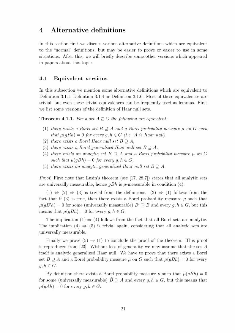
Theorem 4.1.1. For a set A ⊆ G the following are equivalent:

(1) there exists a Borel set B ⊇ A and a Borel probability measure µ on G such

that µ(gBh) = 0 for every g, h ∈ G (i.e. A is Haar null),

(2) there exists a Borel Haar null set B ⊇ A,

(3) there exists a Borel generalized Haar null set B ⊇ A,

(4) there exists an analytic set B ⊇ A and a Borel probability measure µ on G

such that µ(gBh) = 0 for every g, h ∈ G,

(5) there exists an analytic generalized Haar null set B ⊇ A.

Proof. First note that Lusin’s theorem (see [17, 28.7]) states that all analytic sets

are universally measurable, hence gBh is µ-measurable in condition (4).

(1) ⇔ (2) ⇒ (3) is trivial from the definitions. (3) ⇒ (1) follows from the

fact that if (3) is true, then there exists a Borel probability measure µ such that

µ(gB′h) = 0 for some (universally measurable) B′ ⊇ B and every g, h ∈ G, but this

means that µ(gBh) = 0 for every g, h ∈ G.

The implication (1)⇒ (4) follows from the fact that all Borel sets are analytic.

The implication (4) ⇒ (5) is trivial again, considering that all analytic sets are

universally measurable.

Finally we prove (5) ⇒ (1) to conclude the proof of the theorem. This proof

is reproduced from [23]. Without loss of generality we may assume that the set A

itself is analytic generalized Haar null. We have to prove that there exists a Borel

set B ⊇ A and a Borel probability measure µ on G such that µ(gBh) = 0 for every

g, h ∈ G.

By definition there exists a Borel probability measure µ such that µ(gBh) = 0

for some (universally measurable) B ⊇ A and every g, h ∈ G, but this means that

µ(gAh) = 0 for every g, h ∈ G.

21

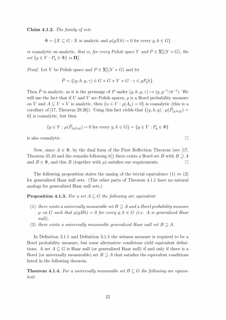
Claim 4.1.2. The family of sets

Φ = {X ⊆ G : X is analytic and µ(gXh) = 0 for every g, h ∈ G}

is coanalytic on analytic, that is, for every Polish space Y and P ∈ Σ11(Y ×G), the

set {y ∈ Y : Py ∈ Φ} is Π11.

Proof. Let Y be Polish space and P ∈ Σ11(Y ×G) and let

P = {(g, h, y, γ) ∈ G×G× Y ×G : γ ∈ gPyh}.

Then P is analytic, as it is the preimage of P under (g, h, y, γ) 7→ (y, g−1γh−1). We

will use the fact that if U and V are Polish spaces, % is a Borel probability measure

on V and A ⊆ U × V is analytic, then {u ∈ U : %(Au) = 0} is coanalytic (this is a

corollary of [17, Theorem 29.26]). Using this fact yields that {(g, h, y) : µ(P(g,h,y)) =

0} is coanalytic, but then

{y ∈ Y : µ(P(g,h,y)) = 0 for every g, h ∈ G} = {y ∈ Y : Py ∈ Φ}

is also coanalytic.

Now, since A ∈ Φ, by the dual form of the First Reflection Theorem (see [17,

Theorem 35.10 and the remarks following it]) there exists a Borel set B with B ⊇ A

and B ∈ Φ, and this B (together with µ) satisfies our requirements.

The following proposition states the analog of the trivial equivalence (1) ⇔ (2)

for generalized Haar null sets. (The other parts of Theorem 4.1.1 have no natural

analogs for generalized Haar null sets.)

Proposition 4.1.3. For a set A ⊆ G the following are equivalent:

(1) there exists a universally measurable set B ⊇ A and a Borel probability measure

µ on G such that µ(gBh) = 0 for every g, h ∈ G (i.e. A is generalized Haar

null),

(2) there exists a universally measurable generalized Haar null set B ⊇ A.

In Definition 3.1.1 and Definition 3.1.4 the witness measure is required to be a

Borel probability measure, but some alternative conditions yield equivalent defini-

tions. A set A ⊆ G is Haar null (or generalized Haar null) if and only if there is a

Borel (or universally measurable) set B ⊇ A that satisfies the equivalent conditions

listed in the following theorem.

Theorem 4.1.4. For a universally measurable set B ⊆ G the following are equiva-

lent:

22

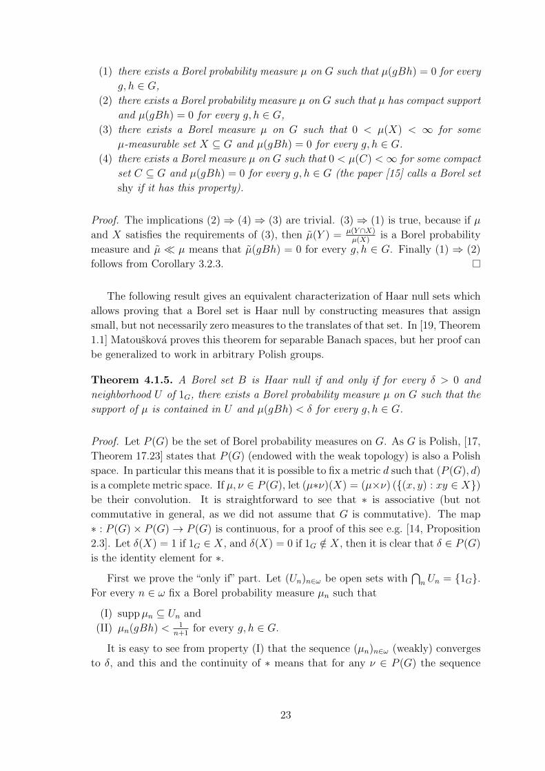
(1) there exists a Borel probability measure µ on G such that µ(gBh) = 0 for every

g, h ∈ G,

(2) there exists a Borel probability measure µ on G such that µ has compact support

and µ(gBh) = 0 for every g, h ∈ G,

(3) there exists a Borel measure µ on G such that 0 < µ(X) < ∞ for some

µ-measurable set X ⊆ G and µ(gBh) = 0 for every g, h ∈ G.

(4) there exists a Borel measure µ on G such that 0 < µ(C) <∞ for some compact

set C ⊆ G and µ(gBh) = 0 for every g, h ∈ G (the paper [15] calls a Borel set

shy if it has this property).

Proof. The implications (2)⇒ (4)⇒ (3) are trivial. (3)⇒ (1) is true, because if µ

and X satisfies the requirements of (3), then µ(Y ) = µ(Y ∩X)µ(X)

is a Borel probability

measure and µ � µ means that µ(gBh) = 0 for every g, h ∈ G. Finally (1) ⇒ (2)

follows from Corollary 3.2.3.

The following result gives an equivalent characterization of Haar null sets which

allows proving that a Borel set is Haar null by constructing measures that assign

small, but not necessarily zero measures to the translates of that set. In [19, Theorem

1.1] Matouskova proves this theorem for separable Banach spaces, but her proof can

be generalized to work in arbitrary Polish groups.

Theorem 4.1.5. A Borel set B is Haar null if and only if for every δ > 0 and

neighborhood U of 1G, there exists a Borel probability measure µ on G such that the

support of µ is contained in U and µ(gBh) < δ for every g, h ∈ G.

Proof. Let P (G) be the set of Borel probability measures on G. As G is Polish, [17,

Theorem 17.23] states that P (G) (endowed with the weak topology) is also a Polish

space. In particular this means that it is possible to fix a metric d such that (P (G), d)

is a complete metric space. If µ, ν ∈ P (G), let (µ∗ν)(X) = (µ×ν) ({(x, y) : xy ∈ X})be their convolution. It is straightforward to see that ∗ is associative (but not

commutative in general, as we did not assume that G is commutative). The map

∗ : P (G)× P (G)→ P (G) is continuous, for a proof of this see e.g. [14, Proposition

2.3]. Let δ(X) = 1 if 1G ∈ X, and δ(X) = 0 if 1G /∈ X, then it is clear that δ ∈ P (G)

is the identity element for ∗.

First we prove the “only if” part. Let (Un)n∈ω be open sets with⋂n Un = {1G}.

For every n ∈ ω fix a Borel probability measure µn such that

(I) suppµn ⊆ Un and

(II) µn(gBh) < 1n+1

for every g, h ∈ G.

It is easy to see from property (I) that the sequence (µn)n∈ω (weakly) converges

to δ, and this and the continuity of ∗ means that for any ν ∈ P (G) the sequence

23

d(ν, ν ∗ µn) converges to zero. This allows us to replace (µn)n∈ω with a subsequence

which also satisfies that d(ν, ν ∗ µn) < 2−n for every measure ν from the finite set

{µj0 ∗ µj1 ∗ . . . ∗ µjr : r < n and 0 ≤ j0 < j1 < . . . < jr < n}.

(Notice that property (II) clearly remains true for any subsequence.) Using this

assumption and the completeness of (P (G), d) we can define (for every n ∈ ω) the

“infinite convolution”µn ∗µn+1 ∗ . . . as the limit of the Cauchy sequence (µn ∗µn+1 ∗µn+2 ∗ . . . ∗ µn+j)j∈ω. We will show that the choice µ = µ0 ∗ µ1 ∗ . . . witnesses that

B is Haar null.

We have to prove that µ(gBh) = 0 for every g, h ∈ G. To show this fix arbitrary

g, h ∈ G and n ∈ ω; we will show that µ(gBh) ≤ 1n+1

. Let αn = µ0 ∗ µ1 ∗ . . . ∗ µn−1

and βn = µn+1 ∗ µn+2 ∗ . . . and notice the continuity of ∗ yields that

µ = limj→∞

(αn ∗ µn ∗ (µn+1 ∗ µn+2 ∗ . . . ∗ µn+j)) =

= (αn ∗ µn ∗ limj→∞

(µn+1 ∗ µn+2 ∗ . . . ∗ µn+j)) = αn ∗ µn ∗ βn.

This means that

µ(gBh) = (αn ∗ µn ∗ βn)(gBh) = (αn × µn × βn)({(x, y, z) ∈ G3 : xyz ∈ gBh}) =

= ((αn × βn)× µn)({((x, z), y) ∈ G2 ×G : y ∈ x−1gBhz−1}).

Notice that for every x, z ∈ G property (II) yields that µn(x−1gBhz−1) < 1n+1

.

Applying Fubini’s theorem in the product space G2 × G to the product measure

(αn × βn)× µn yields that µ(gBh) ≤ 1n+1

.

To prove the “if” part of the theorem, suppose that there exists a δ > 0 and

a neighborhood U of 1G such that for every Borel probability measure µ on G if

suppµ ⊆ U , then µ(gBh) ≥ δ for some g, h ∈ G. Let µ be an arbitrary Borel

probability measure. Applying Lemma 3.2.2 yields that there are a compact set

C ⊆ G and c ∈ G with µ(C) > 0 and C ⊆ cU . Define µ′(X) = µ(cX∩C)µ(C)

, then µ′ is a

Borel probability measure with suppµ′ ⊆ U , hence µ′(gBh) ≥ δ for some g, h ∈ G.

This means that µ(gBh) 6= 0, so µ is not a witness measure for B, and because µ

was arbitrary, B is not Haar null.

For Haar meagerness the following analogue of Theorem 4.1.1 holds:

Theorem 4.1.6. For a set A ⊆ G the following are equivalent:

(1) there exists a Borel set B ⊇ A, a (nonempty) compact metric space K and a

continuous function f : K → G such that f−1(gBh) is meager in K for every

g, h ∈ G (i.e. A is Haar meager),

24

(2) there exists a Borel Haar meager set B ⊇ A,

(3) there exists an analytic set B ⊇ A, a (nonempty) compact metric space K

and a continuous function f : K → G such that f−1(gBh) is meager in K for

every g, h ∈ G.

Proof. (1) ⇔ (2) is trivial from Definition 3.1.6, (1) ⇒ (3) follows from the fact

that all Borel sets are analytic. Finally, the implication (3) ⇒ (1) can be found

as [7, Proposition 8], and the proof is a straightforward analogue of the proof of

(5)⇒ (1) in Theorem 4.1.1.

Without loss of generality we may assume that the set A itself is analytic and

satisfies that f−1(gAh) is meager in K for every g, h ∈ G for some (nonempty)

compact metric space K and continuous function f : K → G. We will prove that

(for this K and f) there exists a Borel set B ⊇ A such that f−1(gBh) is meager in

K for every g, h ∈ G.

Claim 4.1.7. The family of sets

Φ = {X ⊆ G : X is analytic and f−1(gXh) is meager in K for every g, h ∈ G}

is coanalytic on analytic, that is, for every Polish space Y and P ∈ Σ11(Y ×G), the

set {y ∈ Y : Py ∈ Φ} is Π11.

Proof. Let Y be a Polish space and P ∈ Σ11(Y ×G) and let

P = {(g, h, y, k) ∈ G×G× Y ×K : f(k) ∈ gPyh}.

Then P is analytic, as it is the preimage of P under (g, h, y, k) 7→ (y, g−1f(k)h−1).

Novikov’s theorem (see e.g [17, Theorem 29.22]) states that if U and V are Polish

spaces and A ⊆ U×V is analytic, then {u ∈ U : Au is not meager in V } is analytic.

This yields that {(g, h, y) : P(g,h,y) is meager in K} is coanalytic, but then

{y ∈ Y : P(g,h,y) is meager in K for every g, h ∈ G} = {y ∈ Y : Py ∈ Φ}

is also coanalytic.

Now, since A ∈ Φ, by the dual form of the First Reflection Theorem (see [17,

Theorem 35.10 and the remarks following it]) there exists a Borel set B with B ⊇ A

and B ∈ Φ, and this B satisfies our requirements.

To prove our next result we will need a technical lemma. This is a modified

version of the well-known result that for every (nonempty) compact metric space K,

there exists a continuous surjective map ϕ : 2ω → K.

25

Lemma 4.1.8. If (K, d) is a (nonempty) compact metric space, then there exists a

continuous function ϕ : 2ω → K such that if M is meager in K, then ϕ−1(M) is

meager in 2ω.

Proof. We will use a modified version of the usual construction. Note that if

diam(K) < 1, then the ϕ constructed this way will be surjective (we will not need

this).

Let 2<ω =⋃n∈ω 2n be the set of finite 0-1 sequences. The length of a sequence

s is denoted by |s| and the sequence of length zero is denoted by ∅. If s and t are

sequences (where t may be infinite), s � t means that s is an initial segment of t

(i.e. the first |s| elements of t form the sequence s) and s ≺ t means that s � t and

s 6= t. For sequences s, t where |s| is finite, sˆt denotes the concatenation of s and

t. For a finite sequence s, let [s] = {x ∈ 2ω : s � x} be the set of infinite sequences

starting with s. Note that [s] is clopen in 2ω for every s ∈ 2<ω.

We will choose a set of finite 0-1 sequences S ⊆ 2<ω, and for every s ∈ S we

will choose a point ks ∈ K. The construction of S will be recursive: we recursively

define for every n ∈ ω a set Sn and let S =⋃n∈ωSn. Our choices will satisfy the

following properties:

(I) for every n ∈ ω and x ∈ 2ω there exists a unique s = s(x, n) ∈ Sn with s � x,

and s(x, n) ≺ s(x, n′) if n < n′.

(II) for every n ∈ ω and x ∈ 2ω the set Cx,n =⋂

0≤j<nB(ks(x,j),

1j+1

)is nonempty.

First we let S0 = {∅} and choose an arbitrary k∅ ∈ K, then these trivially satisfy

(I) and (II).

Suppose that we already defined S0, S1, . . . , Sn−1 and let s ∈ Sn−1 be arbitrary.

Notice that for x, x′ ∈ [s], Cx,n−1 = Cx′,n−1 and denote this common set with Cs.

The set Cs is (nonempty) compact and it is covered by the open sets {B(c, 1

n

):

c ∈ Cs}, hence we can select a collection (c(s)j )j∈Is where Is is a finite index set such

that⋃j∈Is B

(c

(s)j , 1

n

)⊇ Cs. We may increase the cardinality of this collection by

repeating one element several times if necessary, and thus we can assume that the

index set Is is of the form 2`s for some integer `s ≥ 1 (i.e. it consists of the 0-1

sequences with length `s). Now we can define Sn = {sˆt : s ∈ Sn−1, t ∈ 2`s}. If

s′ ∈ Sn, then there is a unique s ∈ Sn−1 such that s � s′, if t satisfies that s′ = sˆt

(i.e. t is the final segment of s′), then let ks′ = c(s)t .

It is straightforward to check that these choices satisfy (I). Property (II) is sat-

isfied because if x ∈ 2ω, and s, s′ and t are the sequences that satisfy s = s(x, n− 1)

and sˆt = s′ = s(x, n), then ks′ = c(s)t ∈ Cx,n, because it is contained in both

Cx,n−1 = Cs and B(ks′ ,

1n

), and this shows that Cx,n is not empty.

We use this construction to define the function ϕ: let {ϕ(x)} =⋂n∈ω Cx,n (as

the system of nonempty compact sets (Cx,n)n∈ω is descending and diam(Cx,n) ≤

26

diam(B(ks(x,n−1),

1n

))≤ 2 · 1

n→ 0, the intersection of this system is indeed a

singleton). This function is continuous, because if ε > 0 and ϕ(x) = k ∈ K, then

2 · 1n0+1

< ε for some n0, and then for every x′ in the clopen set [s(x, n0)] the set

B(ks(x,n0),

1n0+1

)= B

(ks(x′,n0),

1n0+1

)has diameter < ε and contains both ϕ(x) and

ϕ(x′).

Now we prove that if U ⊆ 2ω is open, then ϕ(U) contains an open set V . It is

clear from (I) that {[s] : s ∈ S} is a base of the topology of 2ω. This means that there

exist a n ∈ ω \ {0} and s ∈ Sn−1 satisfying [s] ⊆ U . Let V =⋂

0≤j<nB(ktj ,

1j+1

)where tj = s(x, j) for an arbitrary x ∈ [s] (this is well-defined as tj ∈ Sj is the

only element of Sj with s(x, j) � s(x, n − 1) = s). It is clear that V is open and

V ⊆ Cx,n−1 = Cs (where x ∈ [s] is arbitrary, this is again well-defined), to show

that V ⊆ ϕ(U) let v ∈ V be arbitrary. Define u0 ∈ 2`s such that v ∈ B(ksˆu0 ,

1n

)(this is possible as {B

(ksˆu0 ,

1n

): u0 ∈ 2`s} was a cover of Cx,n−1 = Cs). Repeat this

to define u1 ∈ 2`sˆu0 such that v ∈ B(ksˆu0ˆu1 ,

1n+1

), then u2 ∈ 2`sˆu0ˆu1 such that

v ∈ B(ksˆu0ˆu1ˆu2 ,

1n+2

)etc. and let y be the infinite sequence y = sˆu0ˆu1ˆu2ˆ . . ..

It is easy to see that ϕ(y) = v, as d(ϕ(y), v) ≤ 2 · 1n+1

for every n ∈ ω.

Finally we show that if M ∈ M(K) is arbitrary, then ϕ−1(M) ∈ M(2ω). As

M is meager M ⊆⋃n∈ω Fn for a system (Fn)n∈ω of nowhere dense closed sets. If

ϕ−1(M) is not meager, then ϕ−1(Fn) contains an open set for some n ∈ ω. But then

Fn contains an open set, which is a contradiction.

We use this lemma to show that in Definition 3.1.6 we can also restrict the choice

of the compact metric space K. In the following theorem the equivalence (1)⇔ (2)

is [8, Proposition 3], the equivalence (1)⇔ (3) is [7, Theorem 2.11].

Theorem 4.1.9. For a Borel set B ⊆ G the following are equivalent:

(1) there exists a (nonempty) compact metric space K and a continuous function

f : K → G such that f−1(gBh) is meager in K for every g, h ∈ G (i.e. B is

Haar meager),

(2) there exists a continuous function f : 2ω → G such that f−1(gBh) is meager

in 2ω for every g, h ∈ G,

(3) there exists a (nonempty) compact set C ⊆ G, a continuous function f : C →G such that f−1(gBh) is meager in C for every g, h ∈ G,

Proof. (1)⇒ (2):

This implication is an easy consequence of Lemma 4.1.8. If K and f satisfies the

requirements of (1) and ϕ is the function granted by Lemma 4.1.8, then f = f ◦ ϕ :

2ω → G will satisfy the requirements of (2), because it is continuous and for every

g, h ∈ G the set f−1(gBh) is meager in K, hence ϕ−1(f−1(gBh)) = f−1(gBh) is

meager in 2ω.

27

(2)⇒ (3):

If G is countable, the only Haar meager subset of G is the empty set. In this case,

any nonempty C ⊆ G and continuous function f : C → G is sufficient. If G is

not countable, then it is well known that there is a (compact) set C ⊆ G that is

homeomorphic to 2ω. Composing the witness function f : 2ω → G granted by (2)

with this homeomorphism yields a function that satisfies our requirements (together

with C).

(3)⇒ (1):

This implication is trivial.

4.2 Coanalytic hulls

In Theorem 4.1.1 and Theorem 4.1.6 we proved that the Borel hull in the definition

of Haar null sets and Haar meager sets can be replaced by an analytic hull. The

following theorems show that it cannot be replaced by a coanalytic hull. As the

proofs of these theorems are relatively long, we do not reproduce them here. Note

that these theorems were proved in the abelian case, but they can be generalized to

the case when G is TSI.

Theorem 4.2.1. (Elekes-Vidnyanszky, see [11]) If G is a non-locally-compact

abelian Polish group, then there exists a coanalytic set A ⊆ G that is not Haar

null, but there is a Borel probability measure µ on G such that µ(gAh) = 0 for every

g, h ∈ G.

Corollary 4.2.2. If G is non-locally-compact and abelian, then GHN (G) %HN (G).

This (and its generalization to TSI groups) is the best known result for the

following question.

Question 4.2.3. (Elekes-Vidnyanszky, see [11, Question 5.4]) Is GHN (G) %HN (G) in all non-locally-compact Polish groups?

Theorem 4.2.4. (Dolezal-Vlasak, see [8]) If G is a non-locally-compact abelian

Polish group, then there exists a coanalytic set A ⊆ G that is not Haar meager, but

there is a (nonempty) compact metric space K and a continuous function f : K → G

such that f−1(gAh) is meager in K for every g, h ∈ G.

4.3 Naive versions

It is possible to eliminate the Borel/universally measurable hull from our definitions

completely. Unfortunately, the resulting “naive” notions will not share the nice

28

properties of a notion of smallness. The results in this subsection will show some of

these problems. Most of these counterexamples are provided only in special groups

or as a corollary of the Continuum Hypothesis, as even these “weak” results are

enough to show that these notions are not very useful.

Definition 4.3.1. A set A ⊆ G is called naively Haar null if there is a Borel

probability measure µ on G such that µ(gAh) = 0 for every g, h ∈ G.

Definition 4.3.2. A set A ⊆ G is called naively Haar meager if there is a

(nonempty) compact metric space K and a continuous function f : K → G such

that f−1(gAh) is meager in K for every g, h ∈ G.

The following two examples show that in certain groups the whole group is the

union of countably many sets which are both naively Haar null and naively Haar

meager, and hence neither the system of naively Haar null sets, nor the system of

naively Haar meager sets is a σ-ideal. The first example is from [9], it uses the

Continuum Hypothesis to partition a group into two naively Haar null sets (hence it

also proves that naively Haar null sets do not form an ideal in this case). The second

example is a certain partition of R2 into countably many sets by Davies (using only

ZFC), where the sets were proved to be naively Haar null in [12, Example 5.4]. In

these papers the sets forming the partitions were only proved to be naively Haar

null, but similar proofs show that they are also naively Haar meager.

Example 4.3.3. Let G be an uncountable Polish group. Assuming the Continuum

Hypothesis, there exists a subset W in the product group G × G such that both W

and (G×G) \W are naively Haar null and naively Haar meager.

Proof. Let <W be a well-ordering of G in order type ω1, and let W = {(g, h) ∈G × G : g <W h} be this relation considered as a subset of G × G. Let µ1 be an

non-atomic measure on G and µ2 be a measure on G that is concentrated on a single

point. It is clear that (µ1×µ2)(gWh) = 0 for every g, h ∈ G (as gWh∩supp (µ1×µ2)

is countable). Similarly (µ2 × µ1)(g((G × G) \W )h) = 0 for every g, h ∈ G, but

these mean that W and (G × G) \ W are both naively Haar null. Let K ⊆ G

be a nonempty perfect compact set (it is well known that such set exists) and let

f1, f2 : K → G be the continuous functions f1(k) = (k, 1G), f2(k) = (1G, k) (here 1Gcould be replaced by any fixed element of G). Then f−1

1 (gWh) is countable (hence

meager) for every g, h ∈ G, so W is naively Haar meager, similarly f2 shows that

(G×G) \W is also naively Haar meager.

Example 4.3.4. The Polish group (R2,+) is the union of countably many sets that

are both naively Haar null and naively Haar meager.

Proof. We use the following result of Davies, its proof can be found in [6].

29

Theorem 4.3.5. Suppose that (θi)i∈ω is a countably infinite system of directions,

such that θi and θj are not parallel if i 6= j. Then the plane can be decomposed as

R2 =⋃i∈ωSi such that each line in the direction θi intersects the set Si in at most

one point.

To prove that in this construction Si is naively Haar null for every i ∈ ω simply

let µi be the 1-dimensional Lebesgue measure on an arbitrary line with direction θi.

Then µi(g+Si + h) = 0 for every g, h ∈ R2, because at most one point of g+Si + h

is contained in the support of µi. This means that Si is indeed naively Haar null.

Similarly let Ki be a nonempty perfect compact subset of an arbitrary line with

direction θi, and let fi : Ki → R2 be the restriction of the identity function. Then

f−1i (g + Si + h) contains at most one point for every g, h ∈ R2, hence it is meager.

This means that Si is indeed naively Haar meager.

The following theorem shows that in a relatively general class of groups the naive

notions are strictly weaker than the corresponding “canonical” notions.

Theorem 4.3.6. Let G be an uncountable abelian Polish group.

(1) There exists a subset of G that is naively Haar null but not Haar null.

(2) There exists a subset of G that is naively Haar meager but not Haar meager.

We do not reproduce the relatively long proof of these results. The proof of

(1) can be found in [12, Theorem 1.3], the proof of (2) can be found in [7, Theo-

rem 16]. Note that when G is non-locally-compact, these results are corollaries of

Theorem 4.2.1 and Theorem 4.2.4.

The following example from [7, Proposition 17] yields the results of Example 4.3.3

in a different class of groups. The cited paper only proves this for the naively Haar

meager case, but states that it can be proved analogously in the naively Haar null

case. We do not reproduce this proof, as it is significantly longer than the proof of

Example 4.3.3.

Example 4.3.7. Let G be an uncountable abelian Polish group. Assuming the Con-

tinuum Hypothesis, there exists a subset X ⊆ G such that both X and G \ X are

naively Haar null and naively Haar meager.

4.4 Left and right Haar null sets

When we defined Haar null sets in Definition 3.1.1, we used multiplication from both

sides by arbitrary elements of G. If we replace this by multiplication from one side,

we get the following notions:

30

Definition 4.4.1. A set A ⊆ G is said to be left Haar null (or right Haar null)

if there are a Borel set B ⊇ A and a Borel probability measure µ on G such that

µ(gB) = 0 for every g ∈ G (µ(Bg) = 0 for every g ∈ G).

Definition 4.4.2. A set A ⊆ G is said to be left-and-right Haar null if there are

a Borel set B ⊇ A and a Borel probability measure µ on G such that µ(gB) =

µ(Bg) = 0 for every g ∈ G.

If “Borel set” is replaced by “universally measurable set”, we can naturally obtain

the generalized versions of these notions. As the papers about this topic happen to

follow Christensen in defining “Haar null set” to mean generalized Haar null set in

the terminology of this thesis, most results in this subsection were originally stated

for these generalized versions.

Notice that even these “one-sided” notions form systems that are translation

invariant, because if e.g. B is Borel left Haar null and a Borel probability measure µ

satisfies µ(gB) = 0 for every g ∈ G and we consider a right translate Bh (this is the

interesting case, invariance under left translation is trivial), then µ′(X) = µ(Xh−1)

is a Borel probability measure which satisfies µ′(g · Bh) = 0 for every g ∈ G. An

analogous argument shows that the system of right Haar null sets is translation

invariant; using Proposition 4.4.7 it follows from these that the system of left-and-

right Haar null sets is also translation invariant. It is clear that this reasoning works

for the generalized versions, too.

Unfortunately, these notions are not “good” notions of smallness in general, be-

cause they fail to form σ-ideals in some groups. In [26] Solecki gives a sufficient

condition which guarantees that the generalized left Haar null sets form a σ-ideal

and gives another sufficient condition which guarantees that the left Haar null sets

do not form a σ-ideal. We state these results and show examples of groups satisfying

these conditions without proofs:

Definition 4.4.3. A Polish group G is called amenable at 1 if for any sequence

(µn)n∈ω of Borel probability measures on G with 1G ∈ suppµn, there are Borel

probability measures νn and ν such that

(I) νn � µn,

(II) if K ⊆ G is compact, then limn(ν ∗ νn)(K) = ν(K).

This class is closed under taking closed subgroups and continuous homomorphic

images. A relatively short proof also shows that (II) is equivalent to

(II’) if K ⊆ G is compact, then limn(νn ∗ ν)(K) = ν(K).

This means that if G is amenable at 1, then so is the opposite group Gopp (Gopp is

the set G considered as a group with (x, y) 7→ y · x as the multiplication).

Examples of groups which are amenable at 1 include:

31

(1) abelian Polish groups,

(2) locally compact Polish groups,

(3) countable direct products of locally compact Polish groups such that all but

finitely many factors are amenable,

(4) inverse limits of sequences of amenable, locally compact Polish groups with

continuous homomorphisms as bonding maps.

Theorem 4.4.4. If G is amenable at 1, then the generalized left Haar null sets form

a σ-ideal.

Our note about the opposite group (and the fact that the intersection of two σ-

ideals is also a σ-ideal) means that generalized right Haar null sets and generalized

left-and-right Haar null sets also form σ-ideals.

The following definition is the sufficient condition for the “bad” case, note that

this condition is also symmetric (in the sense that if G satisfies it, then Gopp also

satisfies it).

Definition 4.4.5. A Polish group G is said to have a free subgroup at 1 if it has a

non-discrete free subgroup whose all finitely generated subgroups are discrete.

The paper [26] mentions several groups which all have a free subgroup at 1, we

mention some of these:

(1) countably infinite products of Polish groups containing discrete free non-

Abelian subgroups,

(2) S∞, the group of all permutations of a countably infinite set,

(3) the group of all permutations of Q which preserve the standard linear order.

Theorem 4.4.6. If G has a free subgroup at 1, then there are a Borel left Haar

null set B ⊆ G and g ∈ G such that B ∪ Bg ∈ G. As the left Haar null sets are

translation invariant and G is not left Haar null, this means that they do not form

an ideal.

As the notion of having a free subgroup at 1 is symmetric, the same is true for

right Haar null sets.

The paper [26] uses these notions for problems related to automatic continuity

and the generalizations of the Steinhaus theorem, in subsection 5.2 we mention a

few of these results.

We finish the examination of these notions with some results about the con-

nections among these notions and the connections between these notions and the

“plain”, two-sided notions defined in subsection 3.1.

It is clear that all Haar null sets are left-and-right Haar null and all left-and-

right Haar null sets are both left Haar null and right Haar null. In abelian groups

32

these notions all trivially coincide with Haar nullness (and the generalized versions

coincide with generalized Haar nullness).

Also note that if A ⊆ G is a conjugacy invariant set (that is, gAg−1 = A for

every g ∈ G), then gAh = gh · h−1Ah = ghA (and similarly gAh = Agh) for every

g, h ∈ G, hence if A is left (or right) Haar null, then A is Haar null.

For locally compact groups Theorem 3.3.7 and the remark in its proof shows

that all generalized right Haar null sets are Haar null. An analogous proof works

for generalized left Haar null sets and thus in locally compact groups eight versions

of Haar null (generalized or not, left or right or left-and-right or “plain”) are all

equivalent to each other and equivalent to having Haar measure zero.

The following simple result mentioned in [22] can be proved by modifying the

proof of [20, Theorem 2]:

Proposition 4.4.7. A set A ⊆ G is left-and-right Haar null if and only if it is both

left Haar null and right Haar null.

Proof. We only have to show that if A is both left Haar null and right Haar null,

then it is left-and-right Haar null, as the other direction is trivial. By definition

there exist a Borel set B ⊇ A and Borel probability measures µ1, µ2 on G such that

µ1(gB) = µ2(Bg) = 0 for every g ∈ G.

Define

µ(X) = (µ1 × µ2)({(x, y) ∈ G2 : yx ∈ X}

),

then µ is clearly a Borel probability measure and if the characteristic function of a

set S is denoted by χS, then using Fubini’s theorem we have

µ(gB) =

∫G

∫G

χgB(yx) dµ1(x) dµ2(y) =

∫G

µ1(y−1gB) dµ2(y) = 0

and

µ(Bg) =

∫G

∫G

χBg(yx) dµ2(y) dµ1(x) =

∫G

µ2(Bgx−1) dµ1(x) = 0

and these show that µ satisfies the requirements of Definition 4.4.2.

There are results that show that (aside from this proposition) the weaker ones

among these notions do not imply the stronger ones.

If G has a free subgroup at 1, Theorem 4.4.6 provides a left Haar null set B

and g ∈ G such that B ∪ Bg ∈ G; this set B is not generalized Haar null as the

generalized Haar null sets form a σ-ideal that does not contain G. Notice that there

are groups that admit a two-sided invariant metric and have a free subgroup at 1

(for example F ω2 where F2 is the free group of rank 2 with discrete topology).

33

In the earlier article [22] Shi and Thompson used more elementary techniques to

find examples in the group H[0, 1] = {f : f is continuous, strictly increasing, f(0) =

0, f(1) = 1} (this is the automorphism group of [0, 1]; the group operation is compo-

sition, the topology is the compact-open topology). We state these results without

proofs:

Example 4.4.8. There exists a Borel set B ⊆ H[0, 1] and a Borel probability mea-

sure µ such that µ(Bg) = 0 for every g ∈ H[0, 1] (this implies that B is right Haar

null), but µ(gB) 6= 0 for some g ∈ H[0, 1] (i.e. µ does not witness that B is left

Haar null).

Example 4.4.9. The group H[0, 1] has a Borel subset that is left-and-right Haar

null but not Haar null.

The following result is [25, Theorem 6.1], a result from another paper of Solecki,

which provides a necessary and sufficient condition for the equivalence of the notions

generalized left Haar null and generalized Haar null in a special class of groups.

Theorem 4.4.10. Let Hn (n ∈ ω) be countable groups and consider the group

G =∏

nHn. The following conditions are equivalent:

(1) In G the system of generalized left Haar null sets is the same as the system of

generalized Haar null sets.

(2) For each universally measurable set A ⊆ G that is not generalized Haar null,

1G ∈ int(AA−1).

(3) For each closed set F ⊆ G that is not (generalized) Haar null, FF−1 is dense

in some non-empty open set.

(4) For all but finitely many n ∈ ω all elements of Hn have finite conjugacy classes

in Hn, that is, for all but finitely many n ∈ ω and for all x ∈ Hn the set

{yxy−1 : y ∈ Hn} is finite.

4.5 Openly Haar null sets

The notion of openly Haar null sets was introduced in [24], and more thoroughly

examined in [4].

Definition 4.5.1. A set A ⊆ G is said to be openly Haar null if there is a Borel

probability measure µ on G such that for every ε > 0 there is an open set U ⊇ A

such that µ(gUh) < ε for every g, h ∈ G. If µ has these properties, we say that µ

witnesses that A is openly Haar null.

The following simple proposition shows that this is a stronger property than

Haar nullness:

34

Proposition 4.5.2. Every openly Haar null set is contained in a Gδ Haar null set.

Proof. For every n ∈ ω there is an open set Un ⊇ A such that µ(gUnh) < 1n+1

for every g, h ∈ G. Then B =⋂n∈ω Un is a Gδ set that is Haar null because it

satisfies µ(gBh) ≤ µ(gUnh) < 1n+1

for every g, h ∈ G, hence µ(gBh) = 0 for every

g, h ∈ G.

To prove that the system of openly Haar null sets forms a σ-ideal, we will need

some lemmas.

Lemma 4.5.3. If µ witnesses that A ⊆ G is openly Haar null and V is a neigh-

borhood of 1G, then there exists a measure µ′ which also witnesses that A is openly

Haar null and has a compact support that is contained in V .

Proof. Lemma 3.2.2 states that there are a compact set C ⊆ G and c ∈ G such that

µ(C) > 0 and C ⊆ cV . Let µ′(X) := µ(cX∩C)µ(C)

, this is clearly a Borel probability

measure and has a compact support that is contained in V . Fix an arbitrary ε > 0.

We will find an open set U ⊇ A such that µ′(gUh) < ε for every g, h ∈ G. Notice

that

µ′(gUh) < ε ⇔ µ(cgUh ∩ C) < µ(C) · ε ⇐ µ(cgUh) < µ(C) · ε.

There exists an open set U ⊇ A with µ(gUh) < µ(C) · ε for every g, h ∈ G, and

this satisfies µ(cgUh) < µ(C) · ε for every g, h ∈ G, hence µ′ has the required

properties.

Theorem 4.5.4. The system of openly Haar null sets is a translation invariant

σ-ideal.

Proof. It is trivial that the system of openly Haar null sets satisfy (I) and (II) in

Definition 3.2.1. The following proof of (III) is described in the appendix of [4] and

is similar to the proof of Theorem 3.2.5.

Let An be openly Haar null for all n ∈ ω, we prove that A =⋃n∈ω An is also

openly Haar null. For every set An fix a measure µn which witnesses that An is

openly Haar null. Let d be a complete metric on G that is compatible with the

topology of G.

We construct for all n ∈ ω a compact set Cn ⊆ G and a Borel probability measure

µn such that the support of µn is Cn, µn(gUnh) < ε for every g, h ∈ G and the “size”

of the sets Cn decreases “quickly”.

The construction will be recursive. For the initial step use Lemma 4.5.3 to find a

measure µ0 witnessing that A0 is openly Haar null and has compact support C0 ⊆ G.

Assume that µn′ and Cn′ are already defined for all n′ < n. By Lemma 3.2.4 there

35

exists a neighborhood Vn of 1G such that if v ∈ Vn, then d(k · v, k) < 2−n for every

k in the compact set C0C1C2 · · ·Cn−1. Applying Lemma 4.5.3 again we can find a

measure µn with compact support Cn ⊆ Vn which is witnessing that An is openly

Haar null.

If cn ∈ Cn for all n ∈ ω, then it is clear that the sequence (c0c1c2 · · · cn)n∈ωis a Cauchy sequence. As (G, d) is complete, this Cauchy sequence is convergent;

we write its limit as the infinite product c0c1c2 · · · . The map ϕ :∏

n∈ω Cn → G,

ϕ((c0, c1, c2, . . .)) = c0c1c2 · · · is the pointwise limit of continuous functions, hence it

is Borel.

Let µΠ be the product of the measures µn on the product space CΠ :=∏

n∈ω Cn.

Let µ = ϕ∗(µΠ) be the push-forward of µΠ along ϕ onto G, i.e.

µ(X) = µΠ(ϕ−1(X)) = µΠ({

(c0, c1, c2, . . .) ∈ CΠ : c0c1c2 · · · ∈ X}).

We claim that µ witnesses that A =⋃n∈ω An is openly Haar null. Fix an

arbitrary ε > 0, we will show that there is an open set U ⊇ A such that µ(gUh) < ε

for every g, h ∈ G. It is enough to find open sets Un ⊇ An such that µ(gUnh) <

ε · 2−(n+2) for every g, h ∈ G and n ∈ ω, because then U =⋃n∈ω Un satisfies that for

every g, h ∈ Gµ(gUh) ≤

∑n∈ω

µ(gUnh) ≤ ε

2< ε.

Fix g, h ∈ G and n ∈ ω. Choose an Un ⊇ An open set satisfying that µn(gUnh) <

ε · 2−(n+2) for every g, h ∈ G. Notice that if cj ∈ Cj for every j 6= n, j ∈ ω, then

µn ({cn ∈ Cn : c0c1c2 · · · cn · · · ∈ gUnh}) =

= µn((c0c1 · · · cn−1)−1 · gUnh · (cn+1cn+2 · · · )−1) < ε · 2−(n+2)

because µn(g′Unh′) < ε · 2−(n+2) for all g′, h′ ∈ G. Applying Fubini’s theorem in the

product space(∏

j 6=nCj

)×Cn to the product measure

(∏j 6=n µj

)× µn yields that

ε · 2−(n+2) > µΠ({

(c0, c1, . . . , cn, . . .) ∈ CΠ : c0c1 · · · cn · · · ∈ gUnh}).

By the definition of µ this means that µ(gUnh) < ε · 2−(n+2).

The surprisingly simple proof of the following result from [4] demonstrates that

this is a useful notion:

Theorem 4.5.5. If there is a nonempty openly Haar null set in G, then every

countable subset C ⊆ G is contained in a comeager Haar null set. In particular, G

may be written as the disjoint union G = A∪B where A is a Haar null set and B is

meager in G.

36

Proof. If there is a nonempty openly Haar null set in G, then applying Lemma 3.2.10

yields that every countable set in G is openly Haar null. In particular a dense

countable set C ′ ⊇ C is openly Haar null. Then Proposition 4.5.2 yields that

C ′ ⊆ A for a Gδ Haar null set A. The dense Gδ set A is a countable intersection of

dense open sets, hence B := G \ A is a countable union of nowhere dense sets, i.e.

B is (Fσ and) meager.

This reasoning shows that a large class of Polish groups can be written as the

union of a Haar null set and a meager set, but unfortunately there are groups where

only the empty set is openly Haar null. We list some results about this in the

following propositions, the proofs of these results can be found in [4].

Proposition 4.5.6. In the Polish group G there is a nonempty openly Haar null

subset if at least one of the following conditions holds:

(1) G is uncountable and admits a two-sided invariant metric,

(2) G = S∞ is the group of permutations of N with the topology of pointwise

convergence,

(3) G = Aut(Q,≤) is the group of order-preserving self-bijections of the rationals

with the topology of pointwise convergence on Q viewed as discrete (i.e. a

sequence (fn)n∈ω ∈ Gω is said to be convergent if for every q ∈ Q there is a

n0 ∈ ω such that the sequence (fn(q))n≥n0 is constant),

(4) G = U(`2) is the unitary group on the separable infinite-dimensional complex

Hilbert space with the strong operator topology,

(5) G admits a continuous surjective homomorphism onto a group listed above.

Proposition 4.5.7. In the Polish group G the empty set is the only openly Haar

null subset if for every compact subset C ⊆ G and every nonempty open subset

U ⊆ G there are g, h ∈ G with gCh ⊆ U . In particular G = H[0, 1], the group

of order-preserving self-homeomorphisms of [0, 1] (endowed with the compact-open

topology) has this property, hence in H[0, 1] only the empty set is openly Haar null.

4.6 Strongly Haar meager sets

Definition 3.1.6 has another interesting version, where we require the witness func-

tion to be the identity function of G restricted to a compact subset C ⊆ G. This

is motivated by the fact that when we prove that some set is Haar meager, we

frequently use witness functions of this kind.

Definition 4.6.1. A set A ⊆ G is said to be strongly Haar meager if there are a

Borel set B ⊇ A and a (nonempty) compact set C ⊆ G such that gBh∩C is meager

in C for every g, h ∈ G.

37

Unfortunately, we know almost nothing about this notion. In [5] Darji asks the

following basic questions for the case when G is abelian (as [5] only considers abelian

groups), but these questions are also interesting in the general case.

Question 4.6.2. Is every Haar meager set strongly Haar meager?

Question 4.6.3. Is the system of strongly Haar meager sets a σ-ideal?

(Of course if the answer for Question 4.6.2 is yes, then the answer for Ques-

tion 4.6.3 is also trivially yes.)

A natural idea for showing that all strongly Haar meager sets are Haar meager

would be showing that if f : K → G is a witness function for a Haar meager set, then

C := f(K) satisfies the requirements of Definition 4.6.1. Unfortunately, this kind of

proof will not work: we reproduce without proof the statement of [5, Example 11],

which shows a Haar meager set where the image of one particular witness function

does not satisfy the requirements of Definition 4.6.1.

Example 4.6.4. There exists a Gδ Haar meager set A ⊆ R, a compact metric space

K and a witness function f : K → R such that A ∩ f(K) is comeager in f(K).

38

5 Analogs of the results from the locally compact

case

In this section we discuss generalizations and analogs of a few theorems that are

well-known for locally compact groups. Unfortunately, although these are true in

locally compact groups for the sets of Haar measure zero and the meager sets, neither

of them remains completely valid for Haar null sets and Haar meager sets. However,

in some cases weakened versions remain true, and these often prove to be useful.

5.1 Fubini’s theorem and the Kuratowski-Ulam theorem

Fubini’s theorem, and its topological analog, the Kuratowski-Ulam theorem (see

e.g. [17, 8.41]) describes small sets in product spaces. They basically state that a

set (which is measurable in the appropriate sense) in the product of two spaces is

small if and only if co-small many sections of it are small. Notice that because the

product of left (or right) Haar measures of two locally compact groups of is trivially

a left (or right) Haar measure of the product group, (a special case of) Fubini’s

theorem connects the sets of Haar measure zero in the two groups and the sets of

Haar measure zero in the product group.

Unfortunately, analogs of these theorems are proved only in very special cases,

and there are counterexamples known in otherwise “nice” groups. We provide a

simple counterexample (which can be found as [7, Example 20]) that works in both

the Haar null and Haar meager case.

Example 5.1.1. There exists a closed set A ⊆ Zω×Zω that is neither Haar null nor

Haar meager, but in one direction all its sections are Haar null and Haar meager.

(In the other direction, non-Haar-null and non-Haar-meager many sections are non-

Haar-null and non-Haar-meager.)

Proof. The group operation of Zω × Zω is denoted by +.

The set with these properties will be

A = {(s, t) ∈ Zω × Zω : tn ≥ sn ≥ 0 for every n ∈ ω}.

It is clear from the definition that A is closed.

Note that for t ∈ Zω, the section At = {s ∈ Zω : tn ≥ sn ≥ 0 for every n ∈ ω}is compact (as it is the product of finite sets with the discrete topology), and it

follows from Theorem 6.3.1 and Corollary 6.3.6 that all compact sets are Haar null

and Haar meager in Zω.

39

To show that A is not Haar null and not Haar meager, we will use the technique

described in subsection 6.5 and show that for every compact set C ⊆ Zω × Zω

the set A contains a translate of C. As C = ∅ satisfies this, we may assume that

C 6= ∅. Let π1n(s, t) = sn and π2

n(s, t) = tn, then π1n, π

2n : Zω × Zω → Z are

continuous functions. Let a and b be the sequences satisfying an = −min π1n(C) and

bn = −minπ2n(C) + maxπ1

n(C)−minπ1n(C). It is straightforward to check that this

choice guarantees that if (s, t) ∈ C + (a, b), then tn ≥ sn ≥ 0 for every n ∈ ω.

Finally, if s ∈ Zω satisfies sn ≥ 0 for every n ∈ ω, then similar, but simpler

arguments show that the section As = {t ∈ Zω : tn ≥ sn for every n ∈ ω} contains

a translate of every compact set C ⊆ Zω, hence it is neither Haar null nor Haar

meager. Similarly, the set {s ∈ Zω : sn ≥ 0 for every n ∈ ω} is also neither Haar

null nor Haar meager, so we proved the statement about the sections in the other

direction.

In [3, Theorem 6] Christensen gives a counterexample for Haar nullness where

one of the two groups in the product is locally compact. We state the properties of

this example without proving them.

Example 5.1.2. Let H be a separable infinite dimensional Hilbert space (with addi-

tion as the group operation) and let S1 be the unit circle in the complex plane (with

complex multiplication as the group operation). There exists in the product group

H × S1 a Borel set A such that

(I) For every h ∈ H, the section Ah has Haar measure one in S1.

(II) For every s ∈ S1, the section As is Haar null in H.

(III) The complement of A is Haar null in the product group H × S1.

The connection between (I) and (III) in this example is not accidental; Chris-

tensen notes that if one of the two groups in a product is locally compact (and both

are abelian), then one direction of Fubini’s theorem holds, that is, a Borel set is

Haar null in the product group if and only if for co-Haar-null many h in the “large”

group, the h-section of the set has Haar measure zero in the locally compact group.

The proof of this remark can be found in [1, Theorem 2.3], we include the proof of

the following generalized version.

Theorem 5.1.3. Suppose that G and H are Polish groups and B ⊆ G×H is a Borel

subset. Then if G is locally compact, then the following conditions are all equivalent.

Moreover, the implication (1)⇒ (2) remains valid even if G is not necessarily locally

compact.

(1) there exists a Haar null set E ⊆ H and a Borel probability measure µ on G

such that every h ∈ H \ E and g1, g2 ∈ G satisfies µ(g1Bhg2) = 0 (i.e. these

sections are Haar null and µ is witness measure for each of them),

40

(2) B is Haar null in G×H,

(3) there exists a Haar null set E ⊆ H such that for every h ∈ H \ E the section

Bh has Haar measure zero in G.

In the theorem equivalence (2)⇔ (3) (which holds when G is locally compact) is

the statement of the remark (generalized for not necessarily abelian groups), condi-

tion (1) is a trivial corollary of (3) that remains meaningful when G is non-locally-

compact and (1) ⇒ (2) is the direction of the remark that remains true when G is

not necessarily locally compact.

Proof. (1)⇒ (2):

As the set E is Haar null, there exists a Borel set E ′ ⊇ E and a Borel probability

measure ν on H such that ν(h1E′h2) = 0 for every h1, h2 ∈ H. We show that the

measure µ× ν witnesses that B is Haar null in G×H. Fix arbitrary g1, g2 ∈ G and

h1, h2 ∈ H, we have to prove that (µ× ν)((g1, h1) ·B · (g2, h2)) = 0.

Notice that

(g1, h1) ·B · (g2, h2) ⊆ (G× (h1 · E ′ · h2)) ∪ ((g1, h1) · (B \ (G× E ′)) · (g2, h2))

and in this union the (µ×ν)-measure of the first term is zero (by the choice of µ and

E ′). For every h ∈ H, the h-section of the Borel set (g1, h1) ·(B\(G×E ′)) ·(g2, h2) is

g1 ·(B\(G×E ′))h−11 hh−1

2 ·g2, and this is either the empty set (if h−11 hh−1

2 ∈ E ′) or a set

of µ-measure zero (if h−11 hh−1

2 ∈ H \E ′). Applying Fubini’s theorem in the product

space G×H to the product measure µ×ν yields that (µ×ν)((g1, h1)·B ·(g2, h2)) = 0,

and this is what we had to prove.

(2)⇒ (3) (when G is locally compact):

Let B ⊆ G×H be Haar null and suppose that µ is a witness measure, i.e. µ((g1, h1) ·B · (g2, h2)) = 0 for every g1, g2 ∈ G and h1, h2 ∈ H. Fix a left Haar measure λ on

G, let δ denote the Dirac measure at 1H (i.e. for X ⊆ H, δ(X) = 1 if 1H ∈ X and

0 otherwise) and let λ = λ× δ. Let E = {h ∈ H : λ(Bh) 6= 0}, it is clearly enough

to prove that E ⊆ H is Haar null. First we use a standard argument to show that

E is a Borel set.

If (X,S) is a measurable space, Y is a separable metrizable space, P (Y ) is the

space of Borel probability measures on Y and A ⊆ X × Y is measurable (i.e. A ∈S ×B(Y )), then [17, Theorem 17.25] states that the map X×P (Y )→ R+, (x, %) 7→%(Ax) is measurable (for S × B(P (Y ))). Applying this for (X,S) := (H,B(H)),

Y := G, and A := B yields that E = {(h, %) ∈ H × P (G) : %(Bh) 6= 0} is Borel (the

Borel preimage of an open set in R+). If % is a Borel probability measure on G that

is equivalent to λ in the sense that they have the same zero sets, then E = E% is

Borel, because it is the section of a Borel set.

41

We will show that the measure ν(X) = µ(G×X) witnesses that E is Haar null.

Fix arbitrary h1, h2 ∈ H, we have to prove that 0 = ν(h1Eh2) = µ(G× (h1Eh2)).

Consider the set

S = {((uG, uH), (vG, vH)) ∈ ((G×H)× (G×H)) :

(uG, uH) · (vG, vH) ∈ (1G, h1) ·B · (1G, h2)},

it is easy to see that this is a Borel set. Applying Fubini’s theorem in the product

space (G×H)× (G×H) to the product measure µ× λ yields that

(µ× λ)(S) =

∫G×H

µ((1G, h1) ·B · (v−1G , h2v

−1H )) dλ((vG, vH)) = 0

because µ witnesses that B is Haar null. Applying Fubini’s theorem again for the

other direction yields that

0 = (µ× λ)(S) =

∫G×H

λ((u−1

G , u−1H h1) ·B · (1G, h2)

)dµ((uG, uH)) =

=

∫G×H

λ({g ∈ G : (g, 1H) ∈ (u−1

G , u−1H h1) ·B · (1G, h2)}

)dµ((uG, uH)) =

=

∫G×H

λ({g ∈ G : (uGg, h

−11 uHh

−12 ) ∈ B}

)dµ((uG, uH)) =

=

∫G×H

λ(u−1G ·B

h−11 uHh

−12

)dµ((uG, uH)) =

∫G×H

λ(Bh−1

1 uHh−12

)dµ((uG, uH)).

It is clear from the definition of E that the function

ϕ : G×H → R+, (uG, uH) 7→ λ(Bh−1

1 uHh−12

)takes strictly positive values on the set G × (h1Eh2). However, our calculations

showed that∫ϕ dµ is zero, hence the µ-measure of the set G × (h1Eh2) must be

zero.

(3)⇒ (1) (when G is locally compact):

Fix a left Haar measure λ on G. (3) states that λ(Bh) = 0 for every h ∈ H \ E.

Using Theorem 3.3.5 it is easy to see that λ(g1Bhg2) = 0 for every g1, g2 ∈ G. Let

C ⊆ G be a Borel set such that 0 < λ(C) <∞ (the regularity of the Haar measure

guarantees a compact C satisfying this) and let µ be the Borel probability measure

µ(X) = λ(X∩C)λ(C)

. Then µ� λ guarantees that µ satisfies condition (1).

We also prove the analog of this for Haar meager sets:

Theorem 5.1.4. Suppose that G and H are Polish groups and B ⊆ G×H is a Borel

subset. Then if G is locally compact, then the following conditions are all equivalent.

42

Moreover, the implication (1)⇒ (2) remains valid even if G is not necessarily locally

compact.

(1) there exists a Haar meager set E ⊆ H, a (nonempty) compact metric space

K and a continuous function f : K → G such that every h ∈ H \ E and

g1, g2 ∈ G satisfies that f−1(g1Bhg2) is meager in K (i.e. these sections are

Haar meager and f is a witness function for each of them),

(2) B is Haar meager in G×H,

(3) there exists a Haar meager set E ⊆ H such that for every h ∈ H \ E the

section Bh is meager in the locally compact group G.

Proof. (1)⇒ (2):

As the set E is Haar meager, there exist a Borel set E ′ ⊇ E, a (nonempty) compact

metric space K ′ and a continuous function ϕ : K ′ → H such that ϕ−1(h1E′h2) is

meager in K ′ for every h1, h2 ∈ H.

Let f × ϕ : K × K ′ → G × H be the function (f × ϕ)(k, k′) = (f(k), ϕ(k′))

(we use this notation because this is the analog of the product measure). We show

that the function f × ϕ witnesses that B is Haar meager in G × H. Fix arbitrary

g1, g2 ∈ G and h1, h2 ∈ H, we have to prove that (f × ϕ)−1((g1, h1) · B · (g2, h2)) is

meager in K ×K ′.

Notice that

(g1, h1) ·B · (g2, h2) ⊆ (G× (h1 · E ′ · h2)) ∪ ((g1, h1) · (B \ (G× E ′)) · (g2, h2))

and in this union

(f × ϕ)−1 (G× (h1 · E ′ · h2)) = K × ϕ−1(h1 · E ′ · h2)

and using the choice of ϕ and the Kuratowski-Ulam theorem it is clear that this

is a meager subset of K × K ′. For every h ∈ H, the h-section of the Borel set

(g1, h1) · (B \ (G × E ′)) · (g2, h2) is g1 · (B \ (G × E ′))h−11 hh−1

2 · g2, and this is either

the empty set (if h−11 hh−1

2 ∈ E ′) or a set whose preimage under f is meager in K (if

h−11 hh−1

2 ∈ H \ E ′). This means that for every k′ ∈ K ′, the k′-section of the set

(f × ϕ)−1 ((g1, h1) · (B \ (G× E ′)) · (g2, h2)) ⊆ K ×K ′

is meager in K. Applying the Kuratowski-Ulam theorem in the product space K×K ′yields that the set (f × ϕ)−1((g1, h1) ·B · (g2, h2)) is indeed meager in K ×K ′, and

this is what we had to prove.

(2)⇒ (3) (when G is locally compact):

Let B ⊆ G × H be Haar meager and suppose that f : K → G × H is a witness

function (where K is a nonempty compact metric space), i.e. f−1((g1, h1)·B ·(g2, h2))

43

is meager in K for every g1, g2 ∈ G and h1, h2 ∈ H. Let f(k) = (fG(k), fH(k)) for

every k ∈ K, then fG : K → G and fH : K → H are continuous functions. Let

E = {h ∈ H : Bh is not meager in G}, then [17, Theorem 16.1] states that E is

Borel. It is enough to prove that E ⊆ H is Haar meager. We show that this is

witnessed by the function fH : K → H. Fix arbitrary h1, h2 ∈ H, we have to prove

that f−1H (h1Eh2) is meager in K.

As in the case of measure, define the Borel set

S = {((uG, uH), (vG, vH)) ∈ ((G×H)× (G×H)) :

(uG, uH) · (vG, vH) ∈ (1G, h1) ·B · (1G, h2)},

and the function ψ : G → G × H, ψ(g) = (g, 1H) (ψ is the analog of λ from the

case of measure). Let f × ψ : K × G → (G × H) × (G × H) be the function

(f × ψ)(k, g) = (f(k), ψ(g)). First notice that for every g ∈ G, the g-section of the

set (f × ψ)−1(S) ⊆ K ×G is

((f × ψ)−1(S))g = {k ∈ K : (f × ψ)((k, g)) ∈ S} =

= {k ∈ K : (f(k), ψ(g)) ∈ S} = {k ∈ K : (f(k), (g, 1H)) ∈ S} =

= {k ∈ K : f(k) ∈ (1G, h1) ·B · (1G, h2) · (g, 1H)−1} =

= f−1((1G, h1) ·B · (g−1, h2))

and this is meager in K (as f witnesses that B is Haar meager), hence the

Kuratowski-Ulam theorem yields that (f × ψ)−1(S) is meager in K ×G.

Applying the Kuratowski-Ulam theorem in the other direction yields that the

set

{k ∈ K : ((f × ψ)−1(S))k is not meager in G}

is meager in K. Here if we let uG = fG(k) and uH = fH(k), then

((f × ψ)−1(S))k = {g ∈ G : (f × ψ)((k, g)) ∈ S} =

= {g ∈ G : (f(k), ψ(g)) ∈ S} = {g ∈ G : ((uG, uH), (g, 1H)) ∈ S} =

= {g ∈ G : (g, 1H) ∈ (uG, uH)−1 · (1G, h1) ·B · (1G, h2)} =

= {g ∈ G : (g, 1H) ∈ (u−1G , u−1

H h1) ·B · (1G, h2)} =

= {g ∈ G : (uGg, h−11 uHh

−12 ) ∈ B} =

= u−1G ·B

h−11 uHh

−12 = (fG(k))−1 ·Bh−1

1 fH(k)h−12 .

Thus we know that

{k ∈ K : (fG(k))−1 ·Bh−11 fH(k)h−1

2 is not meager in G} is meager in K,

44

and because meagerness is translation invariant

{k ∈ K : Bh−11 fH(k)h−1

2 is not meager in G} is meager in K.

But notice that

f−1H (h1Eh2) = {k ∈ K : fH(k) ∈ h1Eh2} = {k ∈ K : h−1

1 fH(k)h−12 ∈ E} =

= {k ∈ K : Bh−11 fH(k)h−1

2 is not meager in G}

so we proved that fH is indeed a witness measure for E.

(3)⇒ (1) (when G is locally compact):

Notice that the proof of Theorem 3.3.13 shows that in a locally compact Polish

group every meager set is Haar meager and there is a function which is a witness

function for each of them. The implication that we have to prove is clearly a special

case of this observation.

Finally, we state another special case when the analog of the Kuratowski-Ulam

theorem is valid. The proof of this result can be found in [7, Theorem 18].

Theorem 5.1.5. Suppose that G and H are Polish groups and A ⊆ G and B ⊆ H

are analytic sets. Then A× B is Haar meager in G×H if and only if at least one

of A and B is Haar meager in the respective group.

5.2 The Steinhaus theorem

The Steinhaus theorem and its generalizations state that if a set A ⊆ G is not

small (and satisfies some measurability condition, e.g. it is in the σ-ideal generated

by the Borel sets and the small sets), then AA−1 = {xy−1 : x, y ∈ A} contains a

neighborhood of 1G.

The original result of Steinhaus stated this in the group (R,+) and used the

sets of Lebesgue measure zero as the small sets. Weil extended this for an arbitrary

locally compact group, using the sets of Haar measure zero as the small sets. We

already stated this result as Corollary 3.3.10 and used a special case of it to prove

that there are no (left or right) Haar measures in non-locally-compact groups.

The proof of Weil’s version also works for non-locally-compact groups, but in

those groups the result is vacuously true, as the statement starts with “If λ is a left

Haar measure on G. . . ”. Using some variant of Haar null sets as the small sets is a

natural idea; this subsection will list some results about these versions.

We already stated the result [25, Theorem 6.1] as Theorem 4.4.10 in the section

about left and right Haar null sets. This theorem shows examples of groups where

45

the straightforward generalization of the Steinhaus theorem using generalized Haar

null sets as small sets is false.

The following positive result can be found as [21, Theorem 2.8] and is a slight

variation of a result in [2]. This result does not claim that AA−1 will be a neigh-

borhood of 1G, only that finitely many conjugates of it will cover a neighborhood

of 1G. Also, it uses generalized right Haar null sets as small sets (see subsection 4.4

for the definition), which is a weaker notion than generalized Haar null sets (hence

this result does not imply the variant where “right” is omitted from the text).

Theorem 5.2.1. Suppose that A ⊆ G is a universally measurable subset which is

not generalized right Haar null. Then for any neighborhood W of 1G there are n ∈ ωand h0, h1, h2, . . . , hn−1 ∈ W such that

h0AA−1h−1

0 ∪ h1AA−1h−1

1 ∪ . . . ∪ hn−1AA−1h−1

n−1

is a neighborhood of 1G.

Proof. This theorem can be found as [21, Theorem 2.8] and it is a slight variation

of a result in [2].

Suppose that the conclusion fails for A and W , that is, for every n ∈ ω and

h0, h1, . . . hn−1 ∈ W and any neighborhood V 3 1G, there is some

g ∈ V \(h0AA

−1h−10 ∪ h1AA

−1h−11 ∪ . . . ∪ hn−1AA

−1h−1n−1

).

Then we can inductively choose a sequence (gj)j∈ω such that gj → 1G and for every

j0 < j1 < j2 < . . . index sequence and r ∈ ω

(I) the infinite product gj0gj1gj2 · · · converges (this can be achieved e.g. by requir-

ing d(gj0 · · · gjr−1 , gj0 · · · gjr−1 · gjr) < 2−jr where d is a fixed complete metric

on G).

(II) gjr /∈ (gj0 · · · gjr−1)−1AA−1(gj0 · · · gjr−1)

Using (I) we can define a continuous map ϕ : 2ω → G by

ϕ(α) = gα(0)0 g

α(1)1 g

α(2)2 · · · ,

where g0 = 1G and g1 = g. Let λ be the Haar measure on the Cantor group

(Z2)ω = 2ω and notice that as A is not generalized right Haar null, there is some

g ∈ G such that

λ(ϕ−1(Ag)) = ϕ∗(λ)(Ag) > 0

So by Corollary 3.3.10,

ϕ−1(Ag)(ϕ−1(Ag))−1

46

contains a neighborhood of the identity (0, 0, . . .) in 2ω. This neighborhood must

contain an element with exactly one “1” coordinate, so there are α, β ∈ ϕ−1(Ag) and

m ∈ ω such that α(m) = 1, β(m) = 0 and α(j) = β(j) for every j ∈ ω, j 6= m. This

means that there are h = gj0gj1 · · · gjr−1 , j0 < j1 < . . . < jr−1 < m and k ∈ G such

that ϕ(α) = hgmk and ϕ(β) = hk. It follows that

hgmh−1 = hgmk · k−1h−1 ∈ Agg−1A = AA−1

and so gm ∈ h−1AA−1h = (gj0 · · · gjr−1)−1AA−1(gj0 · · · gjr−1), contradicting the

choice of gm.

The following special case is often useful:

Corollary 5.2.2. Suppose that A ⊆ G is a universally measurable subset which is

conjugacy invariant (that is, gAg−1 = A for every g ∈ G; in abelian groups every

subset has this property) and not Haar null. Then AA−1 is a neighborhood of the

identity.

Proof. If A is conjugacy invariant, then as we noted, gAh = gAg−1 · gh = Agh

and thus A is generalized right Haar null if and only if A is generalized Haar null.

Moreover, if A is conjugacy invariant, then gAA−1g−1 = (gAg−1) · (gAg−1)−1 =

AA−1, hence AA−1 is also conjugacy invariant and thus in this case Theorem 5.2.1

states that AA−1 is a neighborhood of identity.

Variants of the Steinhaus theorem can be used to prove results about automatic

continuity (results stating that all homomorphisms π : G→ H which satisfy certain

properties are continuous). For example Corollary 3.3.10 yields that any universally

measurable homomorphism from a locally compact Polish group into another Polish

group is continuous (see e.g. [21, Corollary 2.4]; a map is said to be universally

measurable if the preimages of open sets are universally measurable). We prove the

following automatic continuity result as a corollary of Theorem 5.2.1.

Corollary 5.2.3. If G and H are Polish groups, H admits a two-sided invariant

metric and π : G → H is a universally measurable homomorphism, then π is con-

tinuous.

Proof. It is enough to prove that π is continuous at 1G (a homomorphism is con-

tinuous if and only if it is continuous at the identity element). Let V ⊆ H be an

arbitrary neighborhood of 1H .

Using the continuity of the map (x, y) 7→ xy−1 at (1H , 1H) ∈ H ×H, there is an

open set U with 1H ∈ U satisfying that UU−1 ⊆ V . If d is a two-sided invariant

metric on H, then the open balls B(1H , r) are conjugacy invariant sets and form a

neighborhood base of 1H , hence we may also assume that U is conjugacy invariant.

47

G can be covered by countably many right translates of π−1(U), because there is

a countable set S ⊆ π(G) that is dense in π(G) and thus the system {U · s : s ∈ S}covers π(G). This means that the universally measurable set π−1(U) is not right

Haar null, hence we may apply Theorem 5.2.1 to see that for some n ∈ ω and

h0, h1, . . . , hn−1 ∈ G the set

W =⋃

0≤j<n

hjπ−1(U)(π−1(U))−1h−1

j

is a neighborhood of 1G. For every g ∈ W there is a 0 ≤ j < n such that g ∈hjπ

−1(U)(π−1(U))−1h−1j , but then

π(g) ∈ π(hj)UU−1π(hj)

−1 = π(hj)Uπ(hj)−1 · (π(hj)Uπ(hj)

−1)−1 = UU−1,

thus π(W ) ⊆ UU−1 ⊆ V and this shows that π is continuous at 1G.

In [26] Solecki proved that if G is amenable at 1 (see Definition 4.4.3), then a

simpler variant of the Steinhaus theorem is true, but if G has a free subgroup at

1 (see Definition 4.4.5) and satisfies some technical condition, then this variant is

false. The following theorems state these results.

Theorem 5.2.4. If G is amenable at 1 and A ⊆ G is universally measurable and

not generalized left Haar null, then A−1A contains a neighborhood of 1G.

Definition 5.2.5. A Polish group G is called strongly non-locally-compact if for any

neighborhood U of 1G there exists a neighborhood V of 1G such that U cannot be

covered by finitely many sets of the form gV h with g, h ∈ G.

Note that the examples we mentioned after Definition 4.4.5 are all strongly non-

locally-compact.

Theorem 5.2.6. If G has a free subgroup at 1 and is strongly non-locally-compact,

then there is a Borel set A ⊆ G which is not left Haar null and satisfies 1G /∈int(A−1A).

It is possible to prove an analog of the Steinhaus theorem for the case of category,

using the meager sets as the small sets. This result is known as Piccard’s theorem

or as Pettis’ theorem (see e.g. [18, Theorem 2.9.6] and [17, Theorem 9.9]). The

paper [16] generalizes this result to abelian, not necessarily locally compact Polish

groups by proving the analog of the Steinhaus theorem that uses the Haar meager

sets as small sets. We state this theorem without proof; the proof is similar to that

of Theorem 5.2.1 and can be found in [16].

Theorem 5.2.7. Let G be an abelian Polish group. If A ⊆ G is a Borel set that is

not Haar meager, then AA−1 is a neighborhood of 1G.

48

5.3 The countable chain condition

The countable chain condition (often abbreviated as kc) is a well-known property

of partially ordered sets or structures with associated partially ordered sets. A

partially ordered set (P,≤) is said to satisfy the countable chain condition if every

strong antichain in P is countable. (A set A ⊆ P is a strong antichain if ∀x, y ∈A : (x 6= y ⇒ @z ∈ P : (z ≤ x and z ≤ y)).) This is called countable “chain”

condition because in some particular cases this condition happens to be equivalent

to a condition about lengths of certain chains.

We will apply the countable chain condition to notions of smallness in the fol-

lowing sense:

Definition 5.3.1. Suppose that X is a set and S ⊆ A ⊆ P(X). We say that Shas the countable chain condition in A if there is no uncountable system U ⊆ A\Ssuch that U ∩ V ∈ S for any two distinct U, V ∈ U .

In our cases A will be a σ-algebra and S will be the σ-ideal of“small” sets. Notice

that S has the countable chain condition in A if and only if the partially ordered

set (A\S,⊆) satisfies the countable chain condition. Also notice that if S ⊆ S and

A ⊇ A, then “S has the countable chain condition in A” is a stronger statement

than “S has the countable chain condition in A”.

We will generalize the following two classical results (these are stated as [17,

Exercise 17.2] and [17, Exercise 8.31]).

Proposition 5.3.2. If µ is a σ-finite measure, the σ-ideal of sets with µ-measure

zero has the countable chain condition in the σ-algebra of µ-measurable sets.

Proposition 5.3.3. In a second countable Baire space, the σ-ideal of meager sets

has the countable chain condition in the σ-algebra of sets with the Baire property.

The theorems in subsection 3.3 state that if G is locally compact, then N =

HN = GHN (i.e. of Haar measure zero ⇔ Haar null ⇔ generalized Haar null) and

M = HM (i.e. meager ⇔ Haar meager). The special case of Proposition 5.3.2

where µ = λ for a left Haar measure λ on G means that the σ-ideal HN = GNHhas the countable chain condition in the σ-algebra of λ-measurable sets. As every

universally measurable set is λ-measurable, this clearly implies that HN = GHNhas the countable chain condition in the σ-algebra of universally measurable sets.

Analogously, Proposition 5.3.3 means that in a locally compact Polish group G the

σ-ideal HM has the countable chain condition in the σ-algebra of sets with the

Baire property.

For the case of measure Christensen asked in [3, Problem 2] whether is this true

in the non-locally-compact case (the paper [3] considers only abelian groups, but

the problem is interesting in general).

49

The following simple example shows that the answer for this is negative in the

group Zω (a variant of this is stated in [9, Proposition 1]). It also answers the

analogous question in the case of category.

Example 5.3.4. For A ⊆ ω let

S(A) = {s ∈ Zω : sn ≥ 0 if n ∈ A and sn < 0 if n /∈ A}.

Then the system {S(A) : A ∈ P(ω)} consists of continuum many pairwise disjoint

Borel (in fact, closed) subsets of Zω which are neither generalized Haar null nor

Haar meager.

Proof. It is clear that S(A) is closed for every A ⊆ ω. If A and B are two different

subsets of ω, then some n ∈ ω satisfies for example n ∈ A \B and thus ∀s ∈ S(A) :

sn ≥ 0, but ∀s ∈ S(B) : sn < 0.

Finally, for every A ⊆ ω the set S(A) contains a translate of every compact

subset C ⊆ Zω, because if we define t(C) ∈ Zω by

t(C)n =

{min{cn : c ∈ C} if n ∈ A,

−1−max{cn : c ∈ C} if n /∈ A,

then clearly C + t(C) ⊆ A. Applying Lemma 6.5.1 concludes our proof.

In [23] Solecki showed that the situation is the same in all non-locally-compact

groups that admit a two-sided invariant metric. This is a corollary of Theorem 3.3.15,

which we already stated without proof. As we will use Lemma 6.5.1 again, this also

answers the question in the case of category.

Example 5.3.5. Suppose that G is non-locally-compact and admits a two-sided

invariant metric. Then none of HN , GHN and HM has the countable chain con-

dition in B(G).

Proof. By Theorem 3.3.15 there exists a closed set F ⊆ G and a continuous function

ϕ : F → 2ω such that for any x ∈ 2ω and any compact set C ⊆ G there is a

g ∈ G with gC ⊆ ϕ−1({x}). Then the system {ϕ−1({x}) : x ∈ 2ω} consists of

continuum many pairwise disjoint closed sets and they all satisfy the requirements

of Lemma 6.5.1, hence they are neither generalized Haar null nor Haar meager.

50

6 Common techniques

In this section we introduce five techniques, which are frequently useful in practice.

The first four of these can be used to show that a set is small, and the last one can

be used to show that a set is not small. Note that some of the results from the

earlier sections (for example, the basic properties in subsection 3.2 or the equivalent

definitions in subsection 4.1) are also very useful in practice.

6.1 Probes

Probes are a very basic technique for constructing witness measures. The core of

this idea is fairly straightforward and the only surprising thing about probes is the

fact that despite their simplicity they are often useful.

Probes were introduced with the following definition in [15] (this paper examines

the Haar null sets in completely metrizable linear space).

Definition 6.1.1. Suppose that V is an (infinite-dimensional) completely metrizable

linear space. A finite dimensional subspace P ⊆ V is called a probe for a set A ⊆ V

if the Lebesgue measure on P witnesses that A is Haar null.

There is nothing “magical” about this definition, but it is easy to handle these

simple witness measures in the calculations and if there is a probe for a set A ⊇ V ,

then by definition A is Haar null. In arbitrary Polish groups it is easy to generalize

this idea and consider a witness measure which is the “natural” measure supported

on a small and well-understood subgroup or subset. If the considered set and the

candidate for the probe are not too contrived, then it is often easy to see that it is

indeed a probe.

For Haar meager sets the analogue of this is basically proving that the set is

strongly Haar meager (see subsection 4.6) and this is witnessed by a “naturally

chosen” set.

The proof of the following example illustrates the usage of probes. Several more

examples which demonstrate the usage of probes are collected in the paper [15].

Example 6.1.2. In the Polish group (C[0, 1],+) of continuous real-valued functions

on [0, 1], the set M = {f ∈ C[0, 1] : f is monotone on some interval} is Haar null.

Proof. For a proper interval I ⊆ [0, 1] let

M(I) = {f ∈ C[0, 1] : f is monotone on I}.

51

As the Haar null sets form a σ-ideal and

M =⋃{M([q, r]) : 0 ≤ q < r ≤ 1 and q, r ∈ Q},

it is enough to show that M(I) is Haar null for every proper interval I ⊆ [0, 1]. It

is straightforward to check that M(I) is Borel (in fact, closed).

Fix a function ϕ ∈ C[0, 1] such that its restriction to I is not of bounded variation.

We show that the one-dimensional subspace Rϕ = {c · ϕ : c ∈ R} is a probe for

M(I), that is, the measure µ on C[0, 1] that is defined by

µ(X) = λ({c ∈ R : c · ϕ ∈ X})

(where λ is the Lebesgue measure on R) is a witness measure for M(I).

We have to prove that µ(M(I) + f) = 0 for every f ∈ C[0, 1]. By definition

µ(M(I) + f) = λ({c ∈ R : c · ϕ ∈M(I) + f})

and here the set Sf = {c ∈ R : c · ϕ ∈ M(I) + f} has at most one element,

because if c1, c2 ∈ Sf , then c1 · ϕ = m1 + f and c2 · ϕ = m2 + f for some functions

m1,m2 ∈ M(I) that are monotone on I and hence (c1 − c2) · ϕ = m1 − m2 is of

bounded variation when restricted to I, but this is only possible if c1 = c2. Thus

λ(Sf ) = µ(M(I) + f) = 0 and this shows that M(I) is Haar null.

6.2 Application of the Steinhaus theorem

Sometimes the application of one of the results in subsection 5.2 can yield very short

proofs for the Haar nullness and Haar meagerness of certain sets. Unfortunately,

this technique is restricted in the sense that“good”analogs of the Steinhaus theorem

are known only in special groups.

We illustrate this technique by proving Example 6.1.2 again. This new proof

is not as elementary as the one using probes, but also proves that the set under

consideration is Haar meager.

Example 6.2.1. In the Polish group (C[0, 1],+) of continuous real-valued functions

on [0, 1], the set M = {f ∈ C[0, 1] : f is monotone on some interval} is Haar null

and Haar meager.

Proof. As we noted in the proof using probes, if I ⊆ [0, 1] is a proper interval, then

the set

M(I) = {f ∈ C[0, 1] : f is monotone on I}

52

is Borel and it is enough to see that this set is Haar null and Haar meager for every

proper interval I ⊆ [0, 1] (we use the fact that the Haar meager sets also form a

σ-ideal).

Assume for contradiction that there exists a proper interval I ⊆ [0, 1] such

that M(I) is either not Haar null or not Haar meager. If M(I) is not Haar null,

then Corollary 5.2.2 implies that M(I) −M(I) is a neighborhood of the constant

0 function. Similarly, if M(I) is not Haar meager, then Theorem 5.2.7 implies that

M(I)−M(I) is a neighborhood of the constant 0 function.

It is well-known and easy to prove that the difference of two monotone functions is

a function of bounded variation. But M(I)−M(I) is a neighborhood of the constant

0 function and every f ∈M(I)−M(I) satisfies that the restriction f |I is of bounded

variation. This is clearly a contradiction, as it is easy to construct a continuous

function f such that ‖f‖∞ is small and f |I is not of bounded variation.

The proof of Proposition 6.3.2 is another example of this technique.

6.3 Compact sets are small

This technique is based on the idea that in non-locally-compact groups the compact

sets are “small” in the sense that they have empty interior, and in some groups we

can use this to prove other kinds of smallness. The question whether all compact

sets are Haar null and/or Haar meager in some Polish group is interesting on its

own right, and is not yet answered in general.

Several known results state that in groups satisfying certain properties the com-

pact sets are Haar null or Haar meager, and these positive answers are also useful as

lemmas. As both the system of Haar null sets and the system of Haar meager sets

are σ-ideals, these results will also mean that Kσ sets (countable unions of compact

sets) are Haar null and/or Haar meager in these groups.

The following theorem is [9, Proposition 8], one of the earliest results in this

topic.

Theorem 6.3.1. Let G be a non-locally-compact Polish group admitting a two-sided

invariant metric. Then every compact subset of G is Haar null.

Proof. We will use Theorem 4.1.5 to prove this result; this proof is not essentially

different from the proof in [9], but separates the ideas specific to compact sets (this

proof) and the construction of a limit measure (the proof of Theorem 4.1.5).

Fix a two-sided invariant metric d on G and let C ⊆ G be an arbitrary compact

subset. We need to prove that for every δ > 0 and neighborhood U of 1G there

53

exists a Borel probability measure µ on G such that the support of µ is contained

in U and µ(gCh) < δ for every g, h ∈ G.

Fix δ > 0 and a neighborhood U of 1G. We may assume that U is open. As G

is non-locally-compact, the open set U is not totally bounded, hence there exists an

ε > 0 such that U cannot be covered by finitely many open balls of radius 2ε.

As C is compact, hence totally bounded, there exists a N ∈ ω such that C can be

covered by N open balls of radius ε. This means that if X ⊆ C and every x, x′ ∈ Xsatisfies x 6= x′ ⇒ d(x, x′) ≥ 2ε, then |X| ≤ N (because each of the N open balls of

radius ε covering C may contain at most one element of X). Using the invariance

of d this yields that for every g, h ∈ G if X ⊆ gCh and every x, x′ ∈ X satisfies

x 6= x′ ⇒ d(x, x′) ≥ 2ε, then |X| ≤ N .

As U cannot be covered by finitely many open balls of radius 2ε, it is possible

to choose a sequence (un)n∈ω such that un ∈ U and un /∈⋃n−1i=0 B(ui, 2ε) for every

n ∈ ω. Choose an integer M that is larger than Nδ

and let Y = {un : 0 ≤ n < M}.Let µ be the measure on Y which assigns measure 1

Mto every point in Y . If

g, h ∈ G are arbitrary, then µ(gCh) = |gCh∩Y |M

and here every y, y′ ∈ gCh∩Y satisfies

y 6= y′ ⇒ d(y, y′) ≥ 2ε, and hence |gCh ∩ Y | ≤ N , and thus µ(gCh) ≤ NM< δ.

The following result works in all non-locally-compact Polish groups, but only

proves that the compact sets are right Haar null (this is a weaker notion than Haar

nullness, see subsection 4.4 for the definition and properties).

Proposition 6.3.2. Let G be a non-locally-compact Polish group. Then every com-

pact subset of G is right Haar null.

Proof. Suppose that C ⊆ G is compact but not right Haar null. Applying Theo-

rem 5.2.1 yields that there exist a n ∈ ω and h0, h1, . . . , hn−1 ∈ G such that

h0CC−1h−1

0 ∪ h1CC−1h−1

1 ∪ . . . ∪ hn−1CC−1h−1

n−1

is a neighborhood of 1G. But CC−1 is compact (as it is the image of C×C under the

continuous map (x, y) 7→ xy−1), thus its conjugates are also compact, and the union

of finitely many compact sets is also compact, and this is a contradiction, because

a neighborhood cannot be compact in G.

The paper [8] investigates the question in the case of Haar meager sets, we

state the main results without proofs. This article introduces the finite translation

property with the following definition:

Definition 6.3.3. A set A ⊆ G is said to have the finite translation property if

for every open set ∅ 6= U ⊆ G there exists a finite set M ⊆ U such that for every

g, h ∈ G we have gMh * A.

54

The first part of the proof is the following result which allows using this property

to prove that a set is strongly Haar meager (this is a stronger notion than Haar

meagerness, see subsection 4.6 for the definition and properties). The role of this

result is roughly similar to the role of Theorem 4.1.5 in the case of measure; its proof

involves a relatively complex recursive construction.

Theorem 6.3.4. If an Fσ set A ⊆ G has the finite translation property, then A is

strongly Haar meager.

The second part is showing that the compact sets have the finite translation

property when there is a two-sided invariant metric; the proof is relatively simple

and very similar to the one used in Theorem 6.3.1.

Theorem 6.3.5. Let G be a non-locally-compact Polish group admitting a two-sided

invariant metric. Then every compact subset of G has the finite translation property.

These results yield the analogue of Theorem 6.3.1. Note that in the case when

G is abelian, it is also possible to prove this as a corollary of Theorem 5.2.7, using

the method of the proof of Proposition 6.3.2.

Corollary 6.3.6. Let G be a non-locally-compact Polish group admitting a two-sided

invariant metric. Then every compact subset of G is (strongly) Haar meager.

In addition to these, [8] also shows that compact sets have the finite translation

property in the group S∞ of all permutations of a countably infinite set.

We illustrate the usage of this technique with a simple example.

Example 6.3.7. In the non-locally-compact Polish group (Zω,+) there are subsets

A,B ⊆ Zω such that they are neither Haar null nor Haar meager, but for every

x ∈ Zω the intersection (A+ x) ∩B is both Haar null and Haar meager.

Proof. It is well-known that in Zω a closed set C is compact if and only if

C ⊆∏n∈ω

{un, un + 1, un + 2, . . . , vn − 1, vn} for some u, v ∈ Zω,

as sets of this kind are closed subsets in a product of compact sets and in the other

direction if C ⊆ Zω is compact, then the projections map it into compact subsets of

Z.

Let A = {a ∈ Zω : an ≤ 0 for every n ∈ ω} and B = {b ∈ Zω : bn ≥0 for every n ∈ ω}. It is easy to check that these sets satisfy the condition of

Lemma 6.5.1 (the result used in the last technique) and this implies that A and B

are neither Haar null nor Haar meager.

55

On the other hand, the set (A + x) ∩ B = {z ∈ Zω : 0 ≤ zn ≤ xn} is compact,

hence Theorem 6.3.1 and Corollary 6.3.6 shows that it is Haar null and Haar meager.

Note that this phenomenon is impossible in the locally compact case, where non-

small sets have density points and if we translate a density point of one set onto a

density point of the other, then the intersection will be non-small.

6.4 Random construction

This is a technique that is useful when one wants to prove that a not very small

set is Haar null. (For example this does not prove Haar meagerness, hence this can

work for sets that are not Haar meager.) The main idea of this technique is that

a witness measure for a Haar null set A ⊆ G is a Borel probability measure and

one can use the language of probability theory (e.g random variables, conditional

probabilities, stochastic processes) to construct it and prove that it is indeed a

witness measure. For example, the paper [10] applies this to prove a result in S∞,

the group of all permutations of the natural numbers (endowed with the topology of

pointwise convergence). We illustrate this technique by reproducing the core ideas

of this proof. (The proof also contains relatively long calculations which we omit.)

Theorem 6.4.1. In the Polish group S∞ let X be the set of permutations that have

infinitely many infinite cycles and finitely many finite cycles. Then the complement

of X is Haar null.

Proof (sketch). We will find a Borel probability measure µ on S∞ such that

µ(gXh) = 1 for every g, h ∈ S∞. Using that X is conjugacy invariant µ(gXh) =

µ(gh(h−1Xh)) = µ(ghX) and here {gh : g, h ∈ S∞} = S∞ = {g−1 : g ∈ S∞}, thus

it is enough to show that µ(g−1X) = 1 for every g ∈ S∞.

We define the probability measure µ by describing a procedure which chooses a

random permutation p with distribution µ. (This way we can describe a relatively

complex measure in a way that keeps the calculations manageable.)

Fix a sequence k0 < k1 < k2 < . . . of natural numbers which are large enough

(the actual growth rate is used by the omitted parts of the proof). The procedure will

choose values for p(0), p−1(0), p(1), p−1(1), p(2), p−1(2), . . . in this order, skipping

those which are already defined (e.g. if we choose p(0) = 1 in the first step, then the

step for p−1(1) is omitted, as we already know that p−1(1) = 0). When we have to

choose a value for p(n), we choose randomly a natural number n′ < kn which is still

available as an image (that is, n′ ≥ n and n′ is not among the already determined

values p(0), p(1), . . . , p(n−1)); we assign equal probabilities to each of these choices.

Similarly, when we have to choose a value for p−1(n), we choose randomly a natural

56

number n′ ≤ kn which is still available as a preimage (that is, n′ > n and n′ is

not among the already determined values p−1(0), p−1(1), . . . , p−1(n− 1)); we assign

equal probabilities to each of these choices again. When we are finished with these

steps, the resulting object p is clearly a well-defined permutation, as every n ∈ ω

has exactly one image and exactly one preimage assigned to it. We can assume that

kn is large enough to satisfy kn > 2n + 1 and this guarantees that we never “run

out” of choices.

We say that p0 is a possible partial result, if it can arise after finitely many steps

of this process. Relatively long combinatorial arguments show that the following

claim is true:

Claim 6.4.2. Assume that p0 is a possible partial result, g ∈ S∞ is an arbitrary

element and M is a natural number. Then there is a natural number N such that

the conditional probability with respect to µ, under the condition of extending p0, of

the event that the permutation p chosen by our process will be such that gp has

no finite cycles including a number greater than N and no two of the numbers

N + 1, . . . , N +M are in the same cycle of gp is at least 12.

Using this claim, it is possible to show the following claim by induction on i:

Claim 6.4.3. Assume that (as in the previous claim) p0 is a possible partial result,

g ∈ S∞ is an arbitrary element and M is a natural number. Then the conditional

probability (with respect to µ, under the condition of extending p0) of the event that

the permutation p chosen by our process satisfies that gp has only finitely many finite

cycles and at least M infinite cycles is at least 1− 2−i.

Applying this second claim for every i ∈ ω in the special case when p0 is the

empty partial permutation yields that the (unconditional) probability (with respect

to µ) of the event that the permutation p chosen by our process satisfies that gp

has only finitely many finite cycles and at least M infinite cycles is 1. Since this is

true for every M ∈ ω, the permutation gp has infinitely many infinite cycles with

µ-probability 1. This shows that µ(g−1X) = 1 for the arbitrary permutation g, so

we are done.

This set X is the union of countably many conjugacy classes of permutations,

one for each finite list of sizes for the finite cycles in the permutation; the paper [10]

also shows that none of these conjugacy classes are Haar null.

6.5 Sets containing translates of all compact sets

Proving that a set is not Haar null from the definitions requires showing that all

Borel probability measures fail to witness that it is Haar null, which is frequently

harder than just showing one measure witnesses that the set is Haar null. The

57

situation is similar for Haar meager sets, where even the choice of the domain of

the witness function is not straightforward, although the equivalence (1) ⇔ (2) in

Theorem 4.1.9 can be used to eliminate this extra choice. Fortunately, in many cases

the following simple sufficient condition is enough to show that a set is not Haar

null (in fact, not even generalized Haar null) and not Haar meager.

Lemma 6.5.1. Suppose that a set A ⊆ G satisfies that for every compact set C ⊆ G

there are g, h ∈ G such that gCh ⊆ A. Then A is neither generalized Haar null nor

Haar meager.

Proof. This lemma is stated e.g. as [22, Lemma 2.1], but this reasoning is also

frequently used without being stated separately.

If A were generalized Haar null, then by Theorem 4.1.4 there would be an uni-

versally measurable set B ⊇ A and a Borel probability measure µ with compact

support C ⊆ G such that µ(g′Bh′) = 0 for every g′, h′ ∈ G, but there are g, h ∈ Gsuch that gCh ⊆ A ⊆ B and thus µ(g−1Bh−1) ≥ µ(C) = 1, a contradiction.

Similarly, if A would be Haar meager, then there would be a Borel set B ⊇ A,

a (nonempty) compact metric space K and a continuous function f : K → G such

that f−1(g′Bh′) is meager in K for every g′, h′ ∈ G, but there are g, h ∈ G such that

gf(K)h ⊆ A ⊆ B and thus f−1(g−1Bh−1) ⊇ f−1(f(K)) = K is not meager in K, a

contradiction.

58

References

[1] J. M. Borwein, W. B. Moors, Null sets and essentially smooth Lipschitz func-

tions. SIAM J. Optim. 8 (1998), no. 2, 309–323.

[2] J. P. R. Christensen, Borel Structures in Groups and Semigroups. Math. Scand.

28 (1971), 124–128.

[3] J. P. R. Christensen, On sets of Haar measure zero in abelian Polish groups.

Israel J. Math. 13 (1972) 255–260 (1973).

[4] M. P. Cohen, R. R. Kallman, Openly haar null sets and conjugacy in Polish

groups. To appear in Israel J. Math.

[5] U. B. Darji, On Haar meager sets, Topology Appl. 160 (18) (2013) 2396–2400.

[6] R. O. Davies, Covering the plane with denumerably many curves, J. London

Math. Soc. 38 (1963), 433–438.

[7] M. Dolezal, M. Rmoutil, B. Vejnar, V. Vlasak, Haar meager sets revisited. J.

Math. Anal. Appl. 440 (2016), no. 2, 922–939.

[8] M. Dolezal, V. Vlasak, Haar meager sets, their hulls, and relationship to com-

pact sets. Available at arXiv:1603.09510.

[9] R. Dougherty, Examples of non-shy sets. Fund. Math. 144 (1994), 73–88.

[10] R. Dougherty, J. Mycielski, The prevalence of permutations with infinite cycles.

Fund. Math. 144 (1994), no. 1, 89–94.

[11] M. Elekes, Z. Vidnyanszky, Haar null sets without Gδ hulls. Israel J. Math. 209

(1) (2015) 199–214.

[12] M. Elekes, Z. Vidnyanszky, Naively Haar null sets in Polish groups. To appear

in J. Math. Anal. Appl.

[13] E. Hewitt, K. A. Ross, Abstract harmonic analysis. Vol. I. Structure of

topological groups, integration theory, group representations. Second edition.

Grundlehren der Mathematischen Wissenschaften [Fundamental Principles of

Mathematical Sciences], 115. Springer-Verlag, Berlin-New York, 1979.

[14] G. Hognas, A. Mukherjea, Probability measures on semigroups. Convolution

products, random walks, and random matrices. Second edition. Probability and

its Applications (New York). Springer, New York, 2011.

59

[15] B. R. Hunt, T. Sauer, J. A. Yorke, Prevalence: A translation-invariant “almost

every” on infinite-dimensional spaces. Bull. Amer. Math. Soc. (N.S.) 27 (1992),

217–238.

[16] E. Jablonska, Some analogies between Haar meager sets and Haar null sets in

abelian Polish groups. J. Math. Anal. Appl. 421 (2015), no. 2, 1479–1486.

[17] A. S. Kechris, Classical descriptive set theory. Graduate Texts in Mathematics,

156. Springer-Verlag, New York, 1995

[18] M. Kuczma, An Introduction to the Theory of Functional Equations and In-

equalities. Cauchy’s Equation and Jensen’s Inequality. 2nd edition. Birkhauser

Verlag, Basel, 2009, edited by A. Gilanyi.

[19] E. Matouskova, The Banach-Saks property and Haar null sets. Comment. Math.

Univ. Carolin. 39 (1998), no. 1, 71–80.

[20] J. Mycielski, Some unsolved problems on the prevalence of ergodicity, instabil-

ity, and algebraic independence. Ulam Quarterly, 1 (1992), no. 3, 30–37.

[21] C. Rosendal, Automatic continuity of group homomorphisms. Bull. Symbolic

Logic 15 (2009), no. 2, 184–214.

[22] H. Shi, B. S. Thomson, Haar null sets in the space of automorphisms of [0, 1].

Real Anal. Exchange 24 (1998/99), 337–350.

[23] S. Solecki, On Haar null sets. Fund. Math. 149 (1996), no. 3, 205–210.

[24] S. Solecki, Haar null and non-dominating sets. Fund. Math. 170 (2001), 197–217.

[25] S. Solecki, Size of subsets of groups and Haar null sets. Geom. Funct. Anal. 15

(2005), no. 1, 246–273.

[26] S. Solecki, Amenability, free subgroups, and Haar null sets in non-locally com-

pact groups. Proc. London Math. Soc. (3) 93 (2006), no. 3, 693–722.

60