On the Obstacle Problem for the 1D Wave Equation

ON THE OBSTACLE PROBLEM FOR THE 1D WAVE EQUATION

XAVIER FERNANDEZ-REAL AND ALESSIO FIGALLI

A Sandro Salsa per il suo 5014 compleanno, con amicizia ed ammirazione

Abstract. Our goal is to review the known theory on the one-dimensional obstacleproblem for the wave equation, and to discuss some extensions. We introduce the settingestablished by Schatzman within which existence and uniqueness of solutions can beproved, and we prove that (in some suitable systems of coordinates) the Lipschitz normis preserved after collision. As a consequence, we deduce that solutions to the obstacleproblem (both simple and double) for the wave equation have bounded Lipschitz normat all times. Finally, we discuss the validity of an explicit formula for the solution thatwas found by Bamberger and Schatzman.

1. Introduction

1.1. The obstacle problem. Consider an infinite vibrating string represented by itstransversal displacement, u(x, t) ∈ R, with x ∈ R and t ∈ [0,∞), with initial conditionsgiven by {

u(x, 0) = u0(x) for x ∈ Rut(x, 0) = u1(x) for x ∈ R.

Suppose that the string is vibrating freely, but it is restricted to remain above a certaingiven obstacle, which we denote ϕ = ϕ(x) (in particular, we assume u0 ≥ ϕ). Thus, thevibrating string u fulfills the homogeneous wave equation whenever u > ϕ:

�u := utt − uxx = 0 in {u > ϕ}. (1.1)

In order to get a closed system to describe this phenomenon, one also needs to provideinformation regarding the interaction between the string and the obstacle. As we willexplain, a natural condition is to assume that the string bounces elastically at the pointof contact, in the sense that the sign of the velocity is instantly flipped. That is, if (x◦, t◦)is a contact point (i.e., u(x◦, t◦) = ϕ(x◦)), then

ut(x◦, t+◦ ) = −ut(x◦, t−◦ ), (1.2)

where t±◦ denotes taking limits t◦ ± ε as ε ↓ 0.

2010 Mathematics Subject Classification. 35R35, 35L05, 35B65.Key words and phrases. Obstacle problem, wave equation.

1

2 XAVIER FERNANDEZ-REAL AND ALESSIO FIGALLI

Let us assume that the obstacle is given by a wall, so that we can take ϕ ≡ 0. Thisproblem was first studied by Amerio and Prouse in [AP75] in the finite string case (withfixed end-points), constructing a solution “by hand” by following the characteristic curvesand extending the initial condition through the lines of influence. This proved existenceand uniqueness in a “non-standard” class of solutions, by means of very intuitive methods.

A similar approach was used by Citrini in [Cit75] to study properties of solutions (inparticular, the number of times the obstacle is hit) assuming that collisions can lose energyand be either inelastic, partially elastic, or completely elastic, by replacing equation (1.2)with ut(x◦, t

+◦ ) = −hut(x◦, t−◦ ), where h ∈ [0, 1] denotes the loss of energy in each collision.

In this case, its clear that if h < 1 then the local kinetic energy, namely u2t , is no longerpreserved.

In this work we focus on the approach introduced by Schatzman in [Sch80], whereexistence and uniqueness of solutions was proved for a more natural class of solutions(with initial conditions u0 ∈ W 1,2 and u1 ∈ L2). To do so, instead of proceeding with avariational proof, Schatzman explicitly expresses the solution in terms of the free wavewith the same initial data: she adds to the free wave an appropriate measure convolutedwith the fundamental solution of the wave operator, in order to ensure that the specularreflection holds. We show that, at least in the “right” system of coordinates, solutionsbuilt in this way preserve the Lipschitz constant in space-time (see Corollary 3.2). Thisimmediately yields that, even if one considers a second obstacle acting from above (say,ϕ ≡ 1, so that ϕ ≤ u ≤ ϕ for all times), a suitable Lipschitz-type norm of the solutionis constant in time. In particular, solutions remain uniformly Lipschitz independently ofthe number of collisions (see Proposition 4.1).

It is important to notice that, in [BS83], Bamberger and Schatzman studied a penalizedproblem and proved the convergence of solutions to the solution of the obstacle problemfor the wave equation, with general obstacles. In that paper they also gave a simpleexplicit formula for the solution to the obstacle problem when the obstacle is zero, butunfortunately their formula is not correct, as we shall discuss in Section 5.

1.2. Other problems with constrains. The works mentioned so far cover most ofthe literature regarding the obstacle problem in the context of the wave equation, whichis mostly restricted to the one-dimensional case where characteristic equations can beextensively used. The lack of results in higher dimensions or more general obstacles couldbe associated to the need of a more precise model, see Subsection 1.3 below. We hopethat this paper will be of stimulus for investigating these more general problems.

There are also other problems with constrains within the context of hyperbolic equationsthat seem to exhibit cleaner behaviors. In particular, the thin obstacle problem for thewave equation is a simple approximation to the general dynamical Signorini problem. Inthis case, one looks for solutions to the wave equation with a unilateral constrain posed ona lower-dimensional manifold. The problem was original studied by Amerio in [Ame76]and Citrini in [Cit77], and later by Schatzman in [Sch80b], where existence and uniqueness

ON THE OBSTACLE PROBLEM FOR THE 1D WAVE EQUATION 3

is proved: contrary to the obstacle problem presented above, the conservation of energy isa direct consequence of the equations of motion and does not need to be imposed to havea well-posed problem. Later, Kim studied the problem in a variational way in [Kim89],and more recently, even in a non-deterministic approach in [Kim10].

1.3. On the obstacle and the model. As mentioned above, we restrict our attentionto constant obstacles (ϕ ≡ 0). As a direct consequence, our result directly applies if oneconsiders linear obstacles ϕ = ax + b, since �ϕ ≡ 0 and the specular reflection of thewave when hitting obstacle (in the vertical direction) is still preserved. Alternatively, thefunction u− ϕ still presents conservation of energy (see (2.2) below).

Notice, however, that time-dependent obstacles might present added difficulties. Forinstance, even the simple case ϕ = t does not directly follow from our analysis, sincespecular reflection is not preserved if one replaces u by u− t.

In [Sch80] Schatzman studies the case of general convex obstacles (ϕ′′ ≥ 0). Thiscondition is necessary to use the techniques presented there: when the obstacle is notconvex, one could have infinitely many collisions accumulating in space-time to a singlepoint. The convexity of the obstacle ensures that collisions occur only once at each pointin the infinite string case (namely x ∈ R), and that they do not accumulate in time inthe finite string case (namely x ∈ I where I is a bounded interval, and u is fixed on ∂I).In fact, in the infinite string case, one usually expects solutions to diverge to infinity astime goes by (see Remark 5.1).

It is currently unclear how the reflection condition (1.2) should be modified in thegeneral obstacle case. Indeed, one would expect reflections to occur perpendicularly tothe obstacle, rather than vertically. Vertical reflections come from a small oscillationassumption, which is also the same assumption used to derive the wave equation as amodel for a vibrating string (see for instance [PR05, Chapter 1.4.3]). In this sense itis not reasonable to assume non-flat obstacles, and one may wonder whether one canprove existence/uniqueness results assuming small initial data and an obstacle with smalloscillations.

Alternatively, if one wants to impose reflections perpendicular to the obstacle (thushoping to avoid accumulation of collisions), one would need to consider a rotation invariantequation (in the graph space (x, u(x, t)) ∈ R2) instead of the wave equation (compare forinstance [PR05, Equation (1.28) vs (1.29)]). Investigating these modeling questions is avery interesting problem, and we hope that this paper will be a starting point to motivatethis beautiful line of research.

Finally, we should mention that in this paper we consider the model of an infinite string.Nonetheless, the results presented here can be easily extended to the case of a finite stringwith fixed end-points, thanks to the locality of our methods.

Acknowledgment: This work has received funding from the European Research Council(ERC) under the Grant Agreement No 721675.


2. Schatzman’s existence and uniqueness

We consider the zero obstacle case ϕ ≡ 0. Notice that, in the sense of distributions,the support of �u is contained in {u > 0}, and �u ≥ 0. On the other hand, u ≥ 0 byassumption. Our problem can then be written as min{�u, u} = 0 in R× [0,∞)

u(·, 0) = u0 in Rut(·, 0) = u1 in R.

(2.1)

Remark 2.1. Notice that, formally, the formulation above is analogous to the formulationof the parabolic (or elliptic) obstacle problem, which can written as

min{Lu, u− ϕ} = 0

for the corresponding operator (say, L = ∂t − ∆ or L = −∆). In the current situation,however, an extra condition will need to be imposed.

We consider initial data such that u0 ∈ W 1,2loc (R) (in particular, it is continuous) and

u1 ∈ L2loc(R), and we are interested in the existence and uniqueness of solutions in the

natural classu ∈ L∞loc,t((0,∞);W 1,2

loc,x(R)) ∩W 1,∞loc,t((0,∞);L2

loc,x(R)).

That is, for any compact K ⊂⊂ R, and any T > 0,∫K

{|u(x, t)|2 + |ux(x, t)|2 + |ut(x, t)|2

}dx ≤ C(T,K) <∞ for a.e. t ∈ (0, T ),

for some constant C(T,K) independent of t.As mentioned before, we need to provide information regarding the type of reflection

we are expecting. That is, (2.1) is not enough to ensure a unique solution to our problem.In this case, the notion introduced by Schatzman imposes a local energy conservation(corresponding to an elastic collision) in the form

divx,t(−2uxut, u2x + u2t ) =

d

dx(−2uxut) +

d

dt

(u2x + u2t

)= 0 in R× (0,∞), (2.2)

and needs to be understood in the sense of distributions. A posteriori, this notion impliesthat solutions to our problem are elastically reflected, as in (1.2), which is well-definedalmost everywhere. Thus, the equations describing our problem are (2.1)-(2.2).

The main theorem in [Sch80] is then the following:

Theorem 2.2 ([Sch80, Theorem IV.1]). Let u0 ∈ W 1,2loc (R) and u1 ∈ L2

loc(R). Assumethat u0 ≥ 0, and that u1 ≥ 0 a.e. in {u0 = 0}. Then, there exists a unique solutionu ∈ L∞loc,t((0,∞);W 1,2

loc,x(R)) ∩W 1,∞loc,t((0,∞);L2

loc,x(R)) to min{�u, u} = 0 in R× [0,∞)u(·, 0) = u0 in Rut(·, 0) = u1 a.e. in R.

(2.3)


such that (2.2) holds in the sense of distributions.

2.1. Construction of the solution. In order to prove the previous result, Schatzmanbuilds an explicit solution in terms of the free wave equation with the same initial data.Let us denote w the solution to �w = 0 in R× [0,∞)

w(·, 0) = u0 in Rwt(·, 0) = u1 a.e. in R.

(2.4)

If E denotes the fundamental solution to the one-dimensional wave equation, namely

E(x, t) = 121{t≥|x|}, (2.5)

then, by d’Alembert’s formula, w can written as

w = ∂t(E ∗x u0) + E ∗x u1,or more explicitly

w(t, x) =u0(x− t) + u0(x+ t)

2+

1

2

∫ x+t

x−tu1(s) ds for all (x, t) ∈ R× [0,∞).

(see for instance [PR05, Chapter 4]).Let us also denote by T−x,t the cone of dependence of the point (x, t), namely

T−x,t := {(x′, t′) ∈ R× [0,∞) : |x− x′| ≤ t− t′},

and by T+x,t the cone of influence of the point (x, t), that is

T+x,t := {(x′, t′) ∈ R× [0,∞) : |x− x′| ≤ t′ − t}.

One can note that the solution u coincides with w outside the domain of influence of theset of points where w < 0. More precisely, if we denote

E := {(x, t) ∈ R× [0,∞) : w(x, t) < 0} and I =⋃

(x,t)∈E

T+x,t,

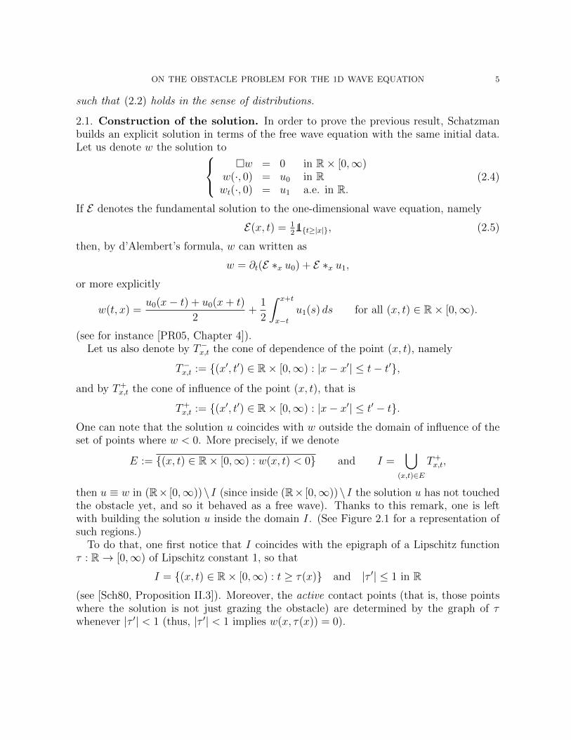
then u ≡ w in (R× [0,∞))\ I (since inside (R× [0,∞))\ I the solution u has not touchedthe obstacle yet, and so it behaved as a free wave). Thanks to this remark, one is leftwith building the solution u inside the domain I. (See Figure 2.1 for a representation ofsuch regions.)

To do that, one first notice that I coincides with the epigraph of a Lipschitz functionτ : R→ [0,∞) of Lipschitz constant 1, so that

I = {(x, t) ∈ R× [0,∞) : t ≥ τ(x)} and |τ ′| ≤ 1 in R

(see [Sch80, Proposition II.3]). Moreover, the active contact points (that is, those pointswhere the solution is not just grazing the obstacle) are determined by the graph of τwhenever |τ ′| < 1 (thus, |τ ′| < 1 implies w(x, τ(x)) = 0).


x

t

E

E

EE

E

I

Figure 2.1. Representation of the regions E where w < 0 and its domainof influence, I.

It is proven in [Sch80] that the solution to (2.3)-(2.2) is given by

u = w + E ∗ µ(w), (2.6)

where µ(w) is the measure defined by the formula

〈µ(w), ψ〉 = −2

∫{x:τ(x)>0}

(1− τ ′(x)2)wt(x, τ(x))ψ(x, τ(x)) dx ∀ψ ∈ Cc(R× [0,+∞)),

and E is as in (2.5).Then, Theorem 2.2 can be proved using the representation (2.6) by checking that such

solution fulfils all the hypotheses.In particular, it is observed that in the infinite string case, the obstacle is touched at

most once at every point x ∈ R (that is, for any x ∈ R, there is at most one time t ∈ [0,∞)such that u(x, t) = 0 and ut(x, t) < 0).

2.2. Formal derivation of (2.6). Let us formally show that the formula (2.6) solves theobstacle problem for the wave equation, in the sense (1.1)-(1.2), for ϕ ≡ 0 (for the actualproof, we refer the reader to [Sch80, Theorem IV.2]).

Let v(x, t) = [E ∗ µ(w)] (x, t), so that

u = w + v.

Since E is the fundamental solution to the one-dimensional wave equation, u solves thewave equation outside

supp(µ(w)) = {(x, τ(x)) : |τ ′(x)| < 1}.Also, one can notice that v ≡ 0 in {t < τ(x)}, and supp(µ(w)) ⊂ {u ≡ 0}.


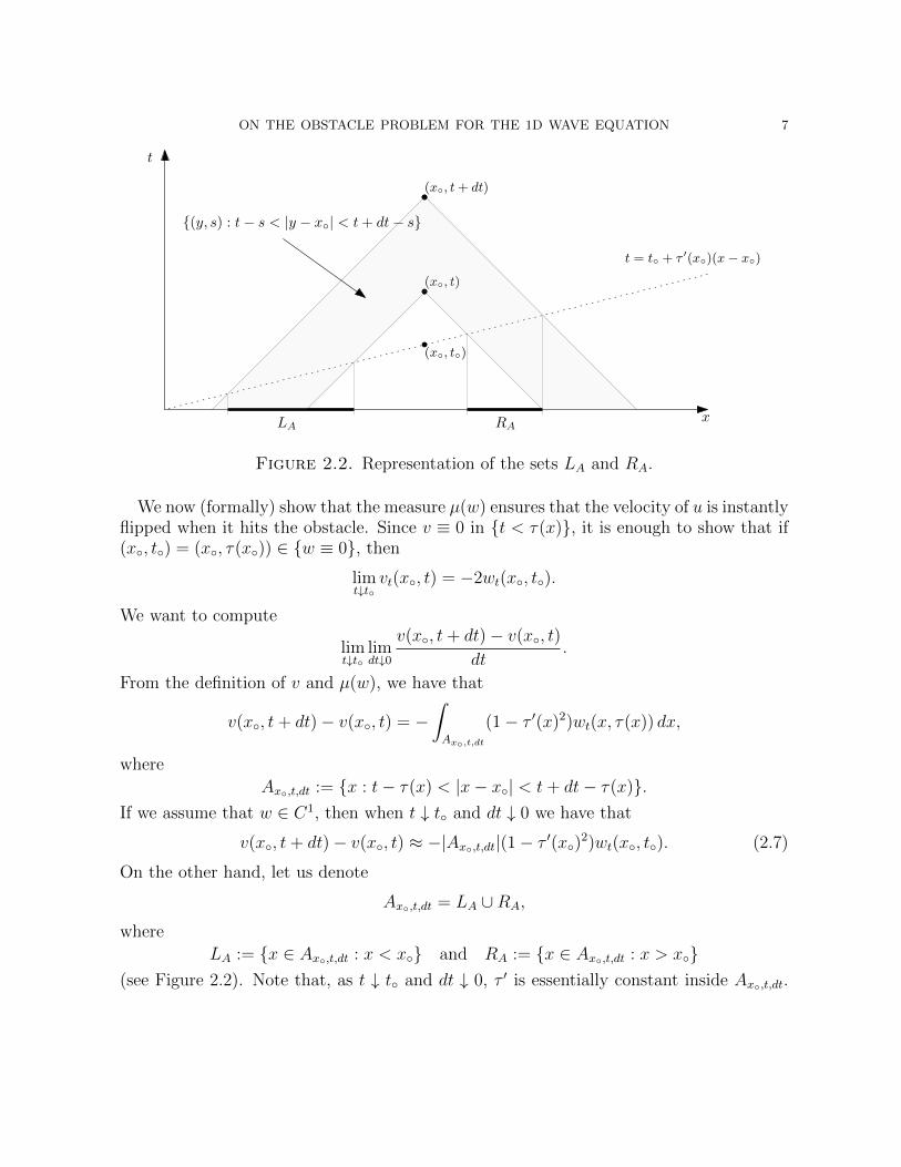
(x◦, t+ dt)

(x◦, t)

(x◦, t◦)

t

x

t = t◦ + τ ′(x◦)(x− x◦)

LA RA

{(y, s) : t− s < |y − x◦| < t+ dt− s}

Figure 2.2. Representation of the sets LA and RA.

We now (formally) show that the measure µ(w) ensures that the velocity of u is instantlyflipped when it hits the obstacle. Since v ≡ 0 in {t < τ(x)}, it is enough to show that if(x◦, t◦) = (x◦, τ(x◦)) ∈ {w ≡ 0}, then

limt↓t◦

vt(x◦, t) = −2wt(x◦, t◦).

We want to compute

limt↓t◦

limdt↓0

v(x◦, t+ dt)− v(x◦, t)

dt.

From the definition of v and µ(w), we have that

v(x◦, t+ dt)− v(x◦, t) = −∫Ax◦,t,dt

(1− τ ′(x)2)wt(x, τ(x)) dx,

where

Ax◦,t,dt := {x : t− τ(x) < |x− x◦| < t+ dt− τ(x)}.If we assume that w ∈ C1, then when t ↓ t◦ and dt ↓ 0 we have that

v(x◦, t+ dt)− v(x◦, t) ≈ −|Ax◦,t,dt|(1− τ ′(x◦)2)wt(x◦, t◦). (2.7)

On the other hand, let us denote

Ax◦,t,dt = LA ∪RA,

where

LA := {x ∈ Ax◦,t,dt : x < x◦} and RA := {x ∈ Ax◦,t,dt : x > x◦}(see Figure 2.2). Note that, as t ↓ t◦ and dt ↓ 0, τ ′ is essentially constant inside Ax◦,t,dt.


Hence, a simple geometric argument yields that

|LA| =dt

1− τ ′(x◦)+ o(dt) and |RA| =

dt

1 + τ ′(x◦)+ o(dt).

Thus,

|Ax◦,t,dt| = |LA|+ |RA| = 2dt

1− τ ′(x◦)2+ o(dt),

and using (2.7) we reach

limt↓t◦

vt(x◦, t) = limt↓t◦

limdt↓0

v(x◦, t+ dt)− v(x◦, t)

dt= −2wt(x◦, t◦)

as desired.This proves that the formula (2.6) guarantees that u flips the velocity when hitting the

obstacle. In order to show that (2.6) gives the solution to the obstacle problem for thewave equation, one still needs to show that u ≥ 0 at all times. This is proved in [Sch80,Proof of Theorem IV.2], using the characteristic variables (see the next section, for adefinition of the characteristic variables). We refer the interested reader to the originalproof.

3. Conservation of the Lipschitz norm

The goal of this section is to describe how the Lipschitz regularity of the solution isaffected by the reflection.

Let x 7→ σ(x) be a non-negative Lipschitz function with |σ′| ≤ 1, and define

v = w + E ∗ µ(w, σ),

where w solves (2.4), and µ(w, σ) is given by

〈µ(w, σ), ψ〉 = −2

∫{x:σ(x)>0}

(1−σ′(x)2)wt(x, σ(x))ψ(x, σ(x)) dx ∀ψ ∈ Cc(R×[0,+∞)).

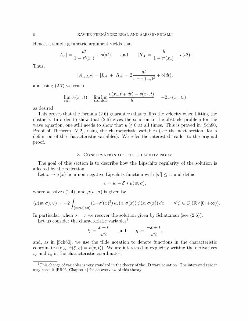
In particular, when σ = τ we recover the solution given by Schatzman (see (2.6)).Let us consider the characteristic variables1

ξ :=x+ t√

2and η :=

−x+ t√2

,

and, as in [Sch80], we use the tilde notation to denote functions in the characteristiccoordinates (e.g. v(ξ, η) = v(x, t)). We are interested in explicitly writing the derivativesvξ and vη in the characteristic coordinates.

1This change of variables is very standard in the theory of the 1D wave equation. The interested readermay consult [PR05, Chapter 4] for an overview of this theory.


x

t

ξη

t = σ(x)

ξ = X(η)η = Y (ξ)

(ξ, η)

(X(η), η)

(ξ, Y (ξ))

xX(η),η xξ,Y (ξ)

Figure 3.3. Representation of σ in characteristic coordinates.

Since σ has Lipschitz constant 1, we can express it as a graph in the (ξ, η)-variables intwo ways: either as (ξ, Y (ξ)) or as (X(η), η). In other words,

η ∈ Y (ξ) ⇔ ξ + η√2

= σ

(ξ − η√

2

)⇔ ξ ∈ X(η).

Note that, at some points, the value of Y or X may not be uniquely determined, sincethese functions may have a vertical segment in their graphs. In this case we shall alwaysrefer to Y (ξ) and X(η) as the unique upper semi-continuous representatives. In otherwords, geometrically, when one take a point (ξ, η) and draws the two lines with slope ±1to find (X(η), η) and (ξ, Y (ξ)), we always choose X(η) and Y (ξ) to be the first point wherethese lines hit the graph of σ (see Figure 3.3). It is important to notice that X = Y −1.

By standard transport along the characteristics one can easily show that

vξ(ξ, η) = wξ(ξ, Y (ξ)) a.e. in {ξ < X(η)},vη(ξ, η) = wη(X(η), η) a.e. in {η < Y (ξ)},

that is, derivatives in ξ are transported along lines of the form {ξ ≡ constant} before thecollision occurs (i.e., in the region where v is a free wave, before the convolution termappears), and analogously for derivatives in η. (This is just a standard consequence ofthe explicit formula for solutions to the wave equations, that in the (ξ, η)-variables readsas wξη = 0.)

On the other hand, derivatives in the remaining region are computed in [Sch80, (III.37)and (III.38)] and are equal to

vξ(ξ, η) = wξ(ξ, Y (ξ))(1− g(ξ))− wη(ξ, Y (ξ))g(ξ) a.e. in {ξ ≥ X(η)}vη(ξ, η) = −wξ(X(η), η)h(η) + wη(X(η), η)(1− h(η)) a.e. in {η ≥ Y (ξ)},


where

g(ξ) =−2Y ′(ξ)

1− Y ′(ξ)1{ξ+Y (ξ)>0} and h(η) =

−2X ′(η)

1−X ′(η)1{X(η)+η>0}

(notice that the indicator functions above represent the region where σ > 0). Equivalently,if we denote

xξ,η :=ξ − η√

2,

we can express the previous derivatives in terms of σ instead of the functions X and Y :

vξ(ξ, η) = wξ(ξ, Y (ξ))σ′(xξ,Y (ξ))− wη(ξ, Y (ξ))(1− σ′(xξ,Y (ξ))) a.e. in {ξ ≥ X(η)}and

vη(ξ, η) = −wξ(X(η), η)(1 + σ′(xX(η),η))− wη(X(η), η)σ′(xX(η),η) a.e. in {η ≥ Y (ξ)}.We have ignored the region where σ = 0 in this case, because a posteriori we will useσ = τ and, thanks to the assumptions in Theorem 2.2, τ(x) > 0 for a.e. x ∈ R.

Proposition 3.1. Under the same assumptions as in Theorem 2.2, the solution of theobstacle problem for the wave equation u fulfills that

|uξ|η ≡ |uη|ξ ≡ 0

a.e. in ξ + η ≥ 0. In particular,

|uξ(x, t)| = |uξ(x+ t, 0)| and |uη(x, t)| = |uη(x− t, 0)|a.e. in t ≥ 0.

Proof. Thanks to the discussion above, by taking σ = τ we are considering the solutionby Schatzman. Thus, we know that

uξ(ξ, η) = wξ(ξ, Y (ξ)) a.e. in {ξ < X(η)}uξ(ξ, η) = wξ(ξ, Y (ξ))τ ′(xξ,Y (ξ))− wη(ξ, Y (ξ))(1− τ ′(xξ,Y (ξ))) a.e. in {ξ ≥ X(η)},

and

uη(ξ, η) = wη(X(η), η) a.e. in {η < Y (ξ)}uη(ξ, η) = −wξ(X(η), η)(1 + τ ′(xX(η),η))− wη(X(η), η)τ ′(xX(η),η)

a.e. in {η ≥ Y (ξ)}.We now notice that, whenever |τ ′(x)| < 1 (that is, at collision points), τ ′(x) can beexpressed in terms of wx(x, τ(x)) and wt(x, τ(x)) as

τ ′(x) = −wx(x, τ(x))

wt(x, τ(x))if |τ ′(x)| < 1.

Using that wx = 1√2

(wξ − wη) and wt = 1√2

(wξ + wη) we obtain that

τ ′(xξ,η) = −wξ(ξ, η)− wη(ξ, η)

wξ(ξ, η) + wη(ξ, η)if

ξ + η√2

= τ

(ξ − η√

2

)and |τ ′(xξ,η)| < 1.


x

t

ξη

t = τ(x)

I1

I1

I1

I2

I3

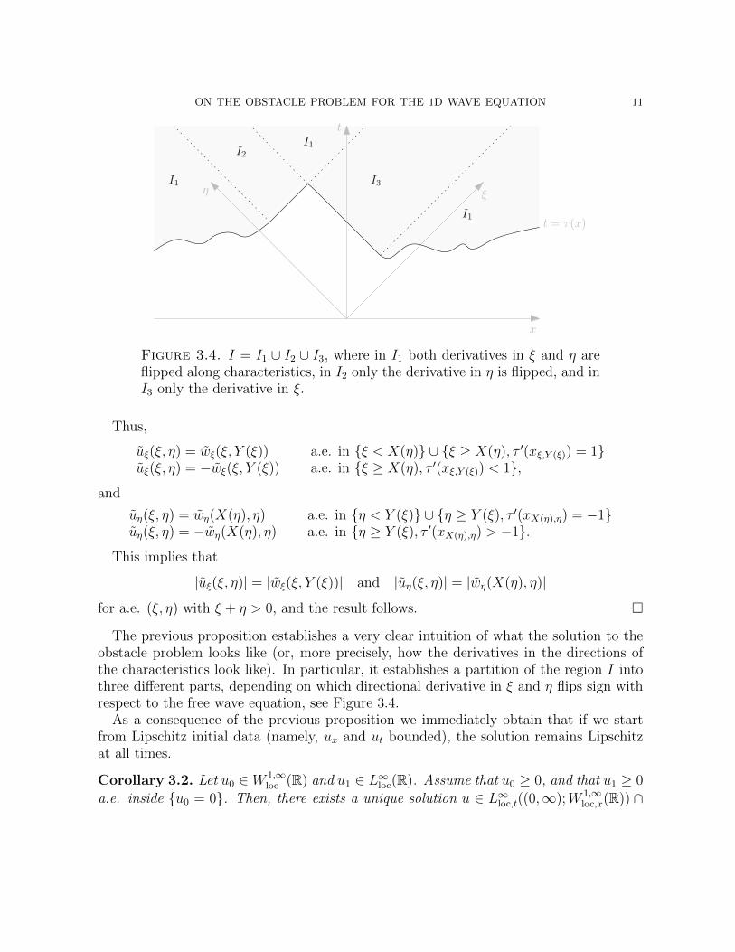
Figure 3.4. I = I1 ∪ I2 ∪ I3, where in I1 both derivatives in ξ and η areflipped along characteristics, in I2 only the derivative in η is flipped, and inI3 only the derivative in ξ.

Thus,

uξ(ξ, η) = wξ(ξ, Y (ξ)) a.e. in {ξ < X(η)} ∪ {ξ ≥ X(η), τ ′(xξ,Y (ξ)) = 1}uξ(ξ, η) = −wξ(ξ, Y (ξ)) a.e. in {ξ ≥ X(η), τ ′(xξ,Y (ξ)) < 1},

and

uη(ξ, η) = wη(X(η), η) a.e. in {η < Y (ξ)} ∪ {η ≥ Y (ξ), τ ′(xX(η),η) = −1}uη(ξ, η) = −wη(X(η), η) a.e. in {η ≥ Y (ξ), τ ′(xX(η),η) > −1}.

This implies that

|uξ(ξ, η)| = |wξ(ξ, Y (ξ))| and |uη(ξ, η)| = |wη(X(η), η)|

for a.e. (ξ, η) with ξ + η > 0, and the result follows. �

The previous proposition establishes a very clear intuition of what the solution to theobstacle problem looks like (or, more precisely, how the derivatives in the directions ofthe characteristics look like). In particular, it establishes a partition of the region I intothree different parts, depending on which directional derivative in ξ and η flips sign withrespect to the free wave equation, see Figure 3.4.

As a consequence of the previous proposition we immediately obtain that if we startfrom Lipschitz initial data (namely, ux and ut bounded), the solution remains Lipschitzat all times.

Corollary 3.2. Let u0 ∈ W 1,∞loc (R) and u1 ∈ L∞loc(R). Assume that u0 ≥ 0, and that u1 ≥ 0

a.e. inside {u0 = 0}. Then, there exists a unique solution u ∈ L∞loc,t((0,∞);W 1,∞loc,x(R)) ∩


W 1,∞loc,t((0,∞);L∞loc,x(R)). Moreover, if u0 ∈ W 1,∞(R) and u1 ∈ L∞(R) then

‖ux(·, t)− ut(·, t)‖L∞(R) = ‖ux(·, 0)− ut(·, 0)‖L∞(R),

‖ux(·, t) + ut(·, t)‖L∞(R) = ‖ux(·, 0) + ut(·, 0)‖L∞(R) for a.e. t ≥ 0.

In particular,

1√2‖∇x,tu(·, 0)‖L∞(R) ≤ ‖∇x,tu(·, t)‖L∞(R) ≤

√2‖∇x,tu(·, 0)‖L∞(R)

for a.e. t ≥ 0.

Proof. The first part is a restatement of Proposition 3.1.For the second part, from Proposition 3.1 and by changing of variables,

|ux(x, t)|2 + |ut(x, t)|2 = |uξ(x, t)|2 + |uη(x, t)|2

= |uξ(x+ t, 0)|2 + |uη(x− t, 0)|2

≤ |ux(x+ t, 0)|2 + |ut(x+ t, 0)|2 + |ux(x− t, 0)|2 + |ut(x− t, 0)|2.

In particular, for every compact set (−L,L) ⊂⊂ R, we are showing that

‖∇x,tu(·, t)‖2L∞((−L,L)) ≤ 2‖∇x,tu(·, 0)‖2L∞((−L−t,L+t)).

Letting L→ +∞, this yields

‖∇x,tu(·, t)‖2L∞(R) ≤ 2‖∇x,tu(·, 0)‖2L∞(R). (3.1)

On the other hand, notice that solutions to the obstacle problem are time-reversible: ifu(x, t) is a solution to an obstacle problem for the wave equation (min{�u, u} = 0 and(2.2) holds), then v(x, t) = u(x, T − t) is also a solution to the obstacle problem for thewave equation. Thus, applying (3.1) to u(·, t− ·) we obtain the desired result. �

4. The double obstacle problem

The previous section not only establishes that the Lipschitz constants of solutions arepreserved at all times (in the characteristic variables), but also shows that, when startingfrom Lipschitz data, the whole problem can be treated at a local level. In particular, thisallows us to treat the double obstacle case, and the same reasoning as before yields thatsolutions to the double obstacle problem preserve the Lipschitz constant (since Proposi-tion 3.1 still holds).

That is, consider now that the solution not only is forced to remain above an obstacleϕ ≡ 0, but also is enclosed to be below ϕ ≡ 1. Locally, when hitting ϕ the solution isbehaving like an obstacle problem for the wave equation (with reverse displacement fromthe previous configuration). Thus, we obtain the validity of the following:


Proposition 4.1. Let u0 ∈ W 1,∞loc (R) and u1 ∈ L∞loc(R). Assume that 0 ≤ u0 ≤ 1, and

that u1 ≥ 0 a.e. inside {u0 = 0} and u1 ≤ 0 a.e. inside {u0 = 1}. Then, there exists aunique solution u ∈ L∞loc,t((0,∞);W 1,∞

loc,x(R)) ∩W 1,∞loc,t((0,∞);L∞loc,x(R)) to

min{�u, u} = 0 in (R× [0,∞)) ∩ {u < 1}min{−�u, 1− u} = 0 in (R× [0,∞)) ∩ {u > 0}

u(·, 0) = u0 in Rut(·, 0) = u1 a.e. in R.

(4.1)

such that (2.2) holds in the sense of distributions. Moreover, if u0 ∈ W 1,∞(R) andu1 ∈ L∞(R) then

‖ux(·, t)− ut(·, t)‖L∞(R) = ‖ux(·, 0)− ut(·, 0)‖L∞(R),

‖ux(·, t) + ut(·, t)‖L∞(R) = ‖ux(·, 0) + ut(·, 0)‖L∞(R).

In particular,

1√2‖∇x,tu(·, 0)‖L∞(R) ≤ ‖∇x,tu(·, t)‖L∞(R) ≤

√2‖∇x,tu(·, 0)‖L∞(R)

for a.e. t ≥ 0.

Proof. Since the initial condition and the solution is locally Lipschitz, the construction ofthe solution by Schatzman as explained above and its properties can also be performed inthis case, locally. In particular, Proposition 3.1 also holds and the desired result followsas in the proof of Corollary 3.2. �

5. An explicit solution by Bamberger and Schatzmam

In [BS83], Bamberger and Schatzman established an explicit formula for the solutionu to the obstacle problem (with zero obstacle) in terms of the free wave solution w. Suchexplicit formula is given by

u(x, t) = w(x, t) + 2 sup(x′,t′)∈T−x,t

(w(x′, t′))−, (5.1)

where r− denotes the negative part, that is r− := sup{−r, 0}. Unfortunately, as we showhere, such formula cannot hold true.

To see that, consider the problem with initial conditions given by u0(x) = 12

andu1(x) = sin(x). The free wave solution is explicit, and is given by

w(x, t) =1

2+ sin(x) sin(t).

In particular, w is bounded and therefore, if the formula above was correct, we woulddeduce that

u ≤ 9

2. (5.2)


Nonetheless, the solution to the obstacle problem in this case goes to infinity as t→∞,a contradiction. Indeed, recalling (2.6), the solution is given by

u(x, t) = w(x, t) + (E ∗ µ(w))(x, t)

with

〈µ(w), ψ〉 = −2

∫(1− τ ′(x)2)wt(x, τ(x))ψ(x, τ(x)) dx ∀ψ ∈ Cc(R× [0,+∞)).

That is,

u(x, t) = w(x, t)−∫{t−τ(z)≥|x−z|}

(1− τ ′(z)2)wt(z, τ(z)) dz.

Notice that, whenever |τ ′(z)| < 1, it holds wt(z, τ(z)) ≤ 0 (since the free wave is touchingthe obstacle ϕ = 0 coming from above). In addition, at x◦ = −π

2we have τ(x◦) = π

6,

τ ′(x◦) = 0, and wt(x◦, τ(x◦)) = 1−√3

2< 0. In particular, by continuity, there exists c◦ > 0

such that ∫ π

−π(1− τ ′(z)2)wt(z, τ(z)) dz = −c◦ < 0.

On the other hand, since the solution is 2π-periodic and τ is 1-Lipschitz, τ ≤ 7π6

. Thus,

u(x, t) ≥ w(x, t)−∫{|z−x|≤t−7π/6}

(1− τ ′(z)2)wt(z, τ(z)) dz.

Hence, by 2π-periodicity of the integrand, if t ≥ 2kπ + 7π6

for some k ∈ N then

u(x, t) ≥ w(x, t) + kc◦,

and letting t→∞ (and, therefore, k →∞) we deduce that u(x, t)→∞ as t→∞. Thisis in contradiction with (5.2), and thus (5.1) cannot hold.

Remark 5.1. In fact, the previous argument shows that solutions with periodic initial dataand with an “active” obstacle (namely, the solutions hit at some moment the obstaclewith positive velocity) will grow to infinity as time goes by, regardless of the form of thesolution.

References

[Ame76] L. Amerio, Su un problema di vincoli unilaterali per l’equazione non omogenea della corda vibrante,Pubbl. IACD, 190 (1976), 3-11.

[AP75] L. Amerio, G. Prouse, Study of the motion of a string vibrating against an obstacle, Rend. Mat. 8 (1975),563-585.

[BS83] A. Bamberger, M. Schatzman, New results on the vibrating string with a continuous obstacle, SIAM J.Math. Anal. 14 (1983), 560-595.

[Cit75] C. Citrini, Sull’urto parzialmente elastico o anelastico di una corda vibrante contro un ostacolo, AttiAccad. Naz. Lincei Rend. Cl. Sci. Fis. Mat. Natur. 59 (1975), 368-376.

[Cit77] C. Citrini, The energy theorem in the impact of a string vibrating against a point-shaped obstacle, Rend.Act. Naz. Lincei, 62 (1977), 143-149.


[Kim89] J. Kim, A boundary thin obstacle problem for a wave equation, Comm. Partial Differential Equations 14(1989), 1011-1026.

[Kim10] J. Kim, On a stochastic wave equation with unilateral boundary conditions, Trans. Amer. Math. Soc. 360(2008), 575-607.

[LS84] G. Lebeau, M. Schatzman, A wave problem in a half-space with a unilateral constraint at the boundary, J.Differential Equations 53 (1984), 309-361.

[PR05] Y. Pinchover, J. Rubinstein, An introduction to partial differential equations, Cambridge University Press,Cambridge, 2005. xii+371 pp.

[Sch80] M. Schatzman, A hyperbolic problem of second order with unilateral constraints: the vibrating string witha concave obstacle, J. Math. Anal. Appl. 73 (1980), 138-191.

[Sch80b] M. Schatzman, Un probleme hyperbolique du 2eme ordre avec contrainte unilaterale: La corde vibranteavec obstacle ponctuel, J. Differential Equations 36 (1980), 295-334.

ETH Zurich, Department of Mathematics, Ramistrasse 101, 8092 Zurich, SwitzerlandE-mail address: [email protected]

ETH Zurich, Department of Mathematics, Ramistrasse 101, 8092 Zurich, SwitzerlandE-mail address: [email protected]

Documents

On the Obstacle Problem for the 1D Wave Equation