APPLIED STOCHASTIC MODELS AND DATA ANALYSIS, VOL. 8, 67-77 (1992)

ON THE NUMERICAL EXPANSION OF A SECOND ORDER STOCHASTIC PROCESS

RAMON GUTIERREZ, JUAN CARLOS RUIZ AND MARIAN0 J . VALDERRAMA

Department of Statistics and Operations Research, University of Granada, 18071 Granada, Spain

SUMMARY

The utility of the classical Karhunen-Loeve expansion of a second order process is limited to its practical derivation, because it depends upon the solution of a Fredholm integral equation associated with it whose kernel is the covariance function of the process. So, in this paper we study two numerical procedures for solving such equations, the Rayleigh-Ritz and the collocation methods, and also essay two different bases of L 2-orthogonal functions in order to perform the algorithms, Legendre polynomials and trigonometric functions, on two well-known processes, the Wiener-Levy process and the Brownian-bridge. The accuracy of the numerical results in relation to the real ones, as well as comparative studies among both procedures are also included.

K E Y WORDS Rayleigh-Ritz method Collocation method Karhunen-Loeve expansion Wiener-Levy process Brownian-bridge

1 . INTRODUCTION

The Karhunen-Lokve (KL) decomposition of a second order continuous process is a very useful tool both in theoretical and practical probabilistic studies as far as the process can be expressed as denumerable series of uncorrelated variables with orthonormal functions as coefficients. So, a real process ( x ( t ) , t 6 [ a , b] 1 with zero-mean and covariance function R(t , s) can be written as

where this series converges in L 2 @ , a, P ) uniformly in quadratic mean in tE [ a , b] , being b

un = 1 @,( t )x ( t ) dt a

a sequence of uncorrelated random variables defined as quadratic mean integrals, and (%(t )] the eigenfunction system associated with the eigenvalues pn of the integral equation

b

a p @ ( t ) = R ( t , s)+(s) ds, a < t < b

8755-O024/92/020067- 1 1 $10.50 01992 by John Wiley & Sons, Ltd.

(3)

Received 6 December 1989 Revised 12 November 1991

68 R. GUTIERREZ, J . c. RUIZ AND M . J . VALDERRAMA

which are L2-orthonormal in the sense that

1 i f m = n 0 i f m s t n s: an(t)a(r) dt =

Some related expansions have been established by Pierre, Masry,’ Cambanis, D e ~ i l l e , ~ Saporta, Adler, and Valderrama. ’

The practical utility of the KL expansion is limited by two essential facts. The first one is that (1) is a series with infinite terms and then when we deal with the truncated expansion at the Nth term we are not considering in fact the actual process but only an approach. Nevertheless, due to the convergence of the series toward the process we can sometimes perform a rigorous treatment with the truncated expansion by bounding the quadratic mean error

N

~ ( t ) = RU, 1) - C pn I ~ t ) 1’ n = l

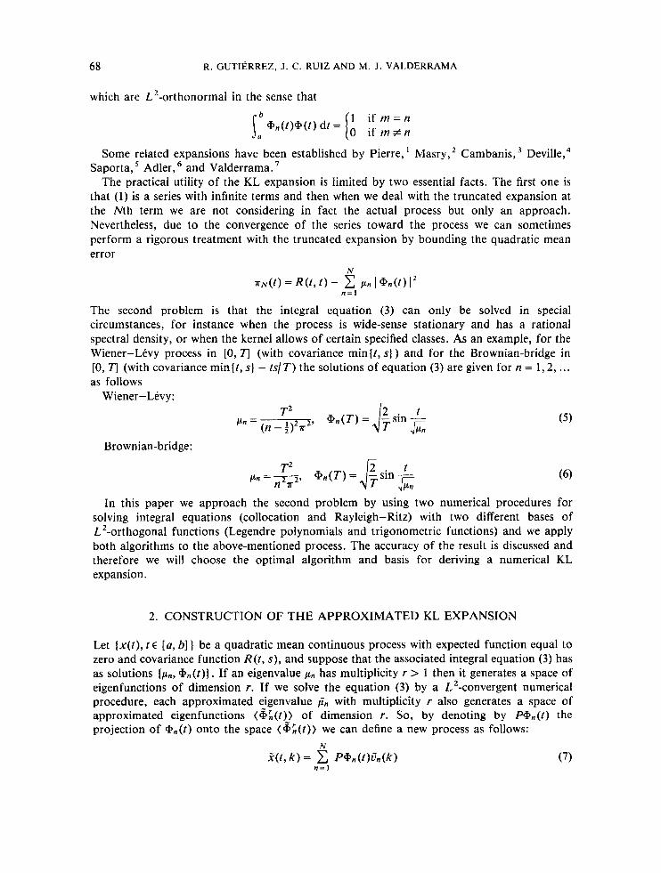
The second problem is that the integral equation (3) can only be solved in special circumstances, for instance when the process is wide-sense stationary and has a rational spectral density, or when the kernel allows of certain specified classes. As an example, for the Wiener-Levy process in [0, T ] (with covariance min ( t , s) ) and for the Brownian-bridge in [0, T j (with covariance min It, sJ - ts/ T ) the solutions of equation (3) are given for n = 1,2, .. . as follows

Wiener-Levy:

Brownian-bridge:

In this paper we approach the second problem by using two numerical procedures for solving integral equations (collocation and Rayleigh-Ritz) with two different bases of L ’-orthogonal functions (Legendre polynomials and trigonometric functions) and we apply both algorithms to the above-mentioned process. The accuracy of the result is discussed and therefore we will choose the optimal algorithm and basis for deriving a numerical KL expansion.

2. CONSTRUCTION OF THE APPROXIMATED KL EXPANSION

Let { x ( t ) , t E [a, b] ) be a quadratic mean continuous process with expected function equal to zero and covariance function R(t, s), and suppose that the associated integral equation (3) has as solutions (pn, (Pn( t ) ) . If an eigenvalue pn has multiplicity r > 1 then it generates a space of eigenfunctions of dimension r. If we solve the equation (3) by a L2-convergent numerical procedure, each approximated eigenvalue En with multiplicity r also generates a space of approximated eigenfunctions (&)‘n(t)) of dimension r. So, by denoting by P+,,(r) the projection of %(t ) onto the space (&)‘n(t)) we can define a new process as follows:

2ND ORDER STOCHASTIC PROCESS NUMERICAL EXPANSION 69

where k is the number of basis functions for the Rayleigh-Ritz method or the number of collocation points (see, as example, Reinhard'), and the random variables U n ( k ) are defined as

b ijn(k) = 1 P + n ( t ) X ( t ) dt

a

Remark

A requisite of the numerical methods, both Rayleigh-Ritz and collocation, is that N < k.

On the basis that the numerical method is convergent, let us show that the process defined in (7) converges towards ( x ( t ) j when N , and then k , grow indefinitely. We denote by 1 1 - 112

the norm in L2 [a, 61 and by 11 * ( I H the norm defined in the minimal space of random variables derived by means of linear operations in the process ( x ( t ) ) as 1 1 X I I H = E [ I X l 2 1 . Then we can write

and both terms trend toward zero when N -+ m.

3. THE RESULTS

For the calculation of the approximated eigenvalues and eigenfunctions we have performed two programs in FORTRAN 77, the first one for the Rayleigh-Ritz method and the second one for the collocation method, and we have used the IMSL library (version 1 .O, April 1987) for integration and eigenvalue routines. On the other hand, a subprogram for the Legendre polynomial multiplication and one for the trigonometric function multiplication, both in [0,1], have been developed. Such programs and subprograms are available to any interested reader. As we said above, the two basic systems employed, with five basic functions, are the Legendre polynomials, that, once normalized in [O, 11, are given by

f d t ) = 1 & ( t ) = 2t - 1 f3(t)=6t2-66t+ 1 f4(t) = 20t3 - 30t2 + 12t - 1 f5(t) = 70t4 - 140f3 + 90t2 - 20t + 1

and the trigonometric functions that, normalized in [0, 11, are

f d t ) = 1 &(f) = cos(27rt) f3(t) = sin(27rt)

f5 (I = sin(4at) f4(f) = COS(4rt)

Table I . Eigenvalues and eigenfunctions for the Wiener-Levy process in [0, I ] by applying the Rayleigh-Ritz method and using a basis of Legendre polynomials

Matrix A

~

Matrix B 1 * 00000 0 * 00000 0 * 00000 0 * 00000 0 * 00000 o*oOoOo 0.33333 0 * 00000 0~00000 0 00000 0~00000 0.0oOoO 0 * 20000 0 * 00000 0~00000 0 * 00000 0~00000 0.00000 0.14286 0~00000 0~00000 0~00000 0~00000 0~00000 0.11111

0 * 00000 0~00000 0.33333 0.08333 - 0,01667 0.00000 0.08333 0.03333 0~00000 - 0.00238

-0.01667 0 00000 0.00476 0~00000 - 0.00079 o.oOoO1 0 00000 - 0.00238 0*00000 0.00159

0.00000 0*00OoO - 0.00079 0*00001 0 *0007 1 0.40528 Eigenvalues 0 * 001 76 0.00674 0.01582 0.04502

Eigenfunctions

d t ( t ) = 0- i2i67fL(t) - o.35615f2(t) + o.63980f3(t) - 0.63994jitt) + I -00ooof5(t) 62( t ) = -0.05666fl(t) + 0*21327fz(t) - 0*04406f3(f) + 0*80136f4(t) + 1.OOOOOfj(t) 63(t) = 0*12455ft(t) - 0*28507f~(t) + 0094742f3(t) + 1 .Ooo00f4(t) - oa70926fj(t) 64(t) = -0.23398fl(t) + l.O0000fz(t) + 0.95248f3(t) - 0*49178fd(t) - 0*17689fs(t) & ( t ) = i.ooooofl(t) + 0-8197if~(t) - o.21849f3(t) - o.03465f4(t) + o.oo387fS(t)

Normalized eigenfunctions (in powers of 2 )

$ l ( t ) = 0*24389t4- 1*11172t3 + 0.06920t2+2*21224f + 2.88101 X $ z ( t ) = - 15*88572t4 + 19.15315t3 + 5-83507t2 - 7.79831t+ 0.04283 +3(t) = -76.52980f4 + 183.88822t3 - 135.87650t2+ 30.72176t - 0.54292 64(t) = 148.69605t4 - 263*34811t3 + 139*55107t2 - 20.58979t - 0.24503 65(t) = 126*01492t4 - 275*07071t3 + 203.49100t'- 58.02162t + 4.96422

Table 11. Eigenvalues and eigenfunctions for the Wiener-Levy process in [0, 11 by applying the collocation method and using a basis of Legendre polynomials

Matrix A

~~

Matrix B 1 ~oO000 -0.90618 0.73 174 - 0.50103 - 0.24574 1 .oOoOo - 0.53487 - 0.06508 0.41738 - 0.34450 1 .OooOo 0~00000 -0.50000 1 *ooOoO 0.53847 - 0.06508 -0.41739 -0.34452

0 - 00000 0.37500

1 * 00000 0.90618 0.73174 0.50104 0.24573 0 * 0458 1 0*00107 - 0*00101 0.0009 1 - O*OoO80 0.2041 4 0.02253 - 0.01576 0.00848 - 0.00270 0.37500 0.08333 - 0.03 125 0 * 00000 0.00521 0.47337 0.1441 4 -0.01576 - 0.00848 - 0.00270 0-49890 0-16556 -0.00101 - 0-00091 - O.OOO80

0.40528 Eigenvalues 0.00241 0.00791 0.01623 0 * 04498 Eigenfunctions

61(t)=0.17489fi(t) -0*5212lf2(t) +0*86636f3(t) -0*99922h(t) + 1-OOOOOf~(t) & ( t ) = -0.02943fi(t) +0*13415f2(f) +0*09597f3(t) +0*69884f4(t)+ 1.00000fs(t) 63(t) = 0*13120f1(t) - 0*30642fz(t) + 0*96368f3(t) + 1 .OOOOOf4(t) - 0*90493f5(t) 64(t) = -0~23395fi(t) + l.O00OOf2(t) + 0*95308f3(t) - 0.49184f4(r)-o.l8726fs(t) & ( t ) = i=ooooofi(t) + 0-81970fi(t) - o.21853f3(t) - 0*03469ji(t) + 0-00392f5(t)

Normalized eigenfunctions (in powers of t )

&l(t)=0.24705t4- 1-11873t3 +0*07411t2 +2-21109t+ 3.42121 x &(t) = - 16*80801t4 + 21 *00278t3 + 4*64213t2 - 7.53372t + 0.03040 * 3 ( t ) = -92*57820t4 + 214.38890t3 - 154*42698t2 + 34.64362t - 0.73598 64(t) = 160*76592t4 - 289*43205t3 + 159.87108t' - 27-37938t+ 0.53638 65(t) = 90.60918t4 - 220.79998t3 + 172.75703t2 - 52.7641 It + 4.91558

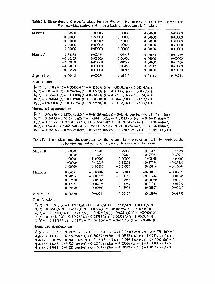
Table 111. Eigenvalues and eigenfunctions for the Wiener-Levy process in [0, 11 by applying the Rayleigh-Ritz method and using a basis of trigonometric functions

Matrix A

Matrix B 1.00000 0.00000 0.00000 0.00000 o ~ m o 0.00000 0.5oooO 0.00000 0.00000 o*ooooo 0.00000 0.00000 0.5oooO 0.00000 0~oooo0 0.00000 0.00000 0.00000 0.5ooOO 0.00000 0.00000 0.00000 0.00000 0.00000 0.00000 0.33333 - 0.02533 - 0.07958 - 0.00633 - 0.03979

- 0.02533 0 *01266 0~oooo0 0.00000 0~oooo0 -0.07958 0.00000 0.03799 0.00000 0.0 1266 - 0.00633 0.00000 0.00000 0.00317 O*OOOOO -0.03979 0.00000 0.01 266 0.00000 0.00950

Eigenvalues 0.00443 0.00784 0.01 543 0.043 I 5 0 * 3891 3

Eigenfunctions

6~(t)=0.14989f1(t)+0-36338f2(f)+0*11304f3(t)+ 1*00000f,(t) +0*62244f5(t) & ( t ) = o.08540f1(t) + 0*24734f~(t) - 0*17223f3(t) - Oa71845f4(f) + I . ~ f s ( t ) %3(t) =0.19542fi(t) + 1*00000fz(t) +0*66483f~(t) -0.27201f4(?)-0.36164f5(t) @ 4 ( f ) = o-24484fi(t) - 0*69590fi(t) + 1 * m j 3 ( t ) - O*O8421f4(l) - 0'24203fs(t) 6s(t ) = I .00000fi(t) - 0*13925fi(t) - 0.52858f3(t) - 0*03308f4(t) t 0.25117f~(t)

Normalized eigenfunctions

= 0-91996 - 0.12810 cos(2st) - 0.48629 sin(2rt) - 0.03042 cos(4nt) - 0.23107 sin(4st) % 2 ( t ) = 0.26795 - 0.76159 cos(2st) + 1-0944 sin(2rt) - 0.09215 cos (4st) + 0.26487 sin(4st) ? 3 ( t ) = 0.21053 + 1 e07734 cos(2st) + 0.71624 sin(2rt) - 0.29304 cos(4st) - 0.3896 sin(4st) ? 4 ( t ) = 0-9484 + 0,27468 cos(2st) + 0.19127 sin(2st) - 0.79788 cos (47rt) + 1 *11056 sin(4st) aS(f) = 0.16878 + 0.40919 cos(2xt) + 0.12729 sin(2st) t 1.12609 cos (4st) t 0.70092 sin(4rf)

Table IV. Eigenvalues and eigenfunctions for the Wiener-Levy process in [0,1] by applying the collocation method and using a basis of trigonometric functions

Matrix A

Matrix B 1 . m o 0-95688 0.29050 0 - 83 123 0.55594 1.00000 0.12059 0.99270 - 0.97091 0-23943 1.00000 -1.00000 o ~ m o 1 .00OOo o*ooOOo 1 -00000 0.12053 -0.99271 - 0.97094 - 0.23931 1.00000 0.95686 - 0.29055 0.831 16 - 0.55604

-0*00109 -0.O0011 -0.00107 -0.00021 0.20414 - 0.02228 - 0.01 158 -0.01244 - 0.01685 0.37500 - 0.05066 -0.07958 0-ooooo - 0-03979

- 0.06272 0.47337 - 0.02228 -0.14757 -0.01244 0.49890 -0*00109 -0.15905 -0.00107 -0.07937

0 * 0458 1

0.39730 Eigenvalues 0*00360 0.00945 0 02 175 0 * 03976

Eigenfunctions

6 l ( f ) = 0.17083fi(t) + 0*42058f2(t) + 0*01435f3(t) + 0.75708f4(?) + 1 *00000fs(t) 6 2 ( t ) = 0.14512fr(t) + 0.48739fi(t) - 0.01932f3(t) - 0*56369f4(t) + 1 .-f5(1)

& 4 ( f ) = 0.15433fi(t) - 0*57429fz(f) + 0.25715f3(t) - 0*05556f4(f) + l . m f s ( t ) 6s(t) = -0*81887fi(f) + 0-11779f2(t) +0'11662f3(t) +0*02523&(f) + I . W f s ( t )

6,( t) = -o.03244fi(t) - o.47935f2(t) - 047640f3(t) + o.02516f4(t) + l . m f s ( t )

Normalized eigenfunctions

Hl ( t ) = -0.75236 + 0.10822 cos(2st) +0.10714 sin(2rt) + 0-02318 cos(4st) + 0-91878 sin(4st) a2(t) =0-18146 - 0-67524 cos(2st) + 0.30235 sin(2rf) - 0-06532 cos(4st) + 1.17579 sin(4st) 6,(t) = -0.03797 - 0.56113 cos(2at) - 0.55768 sin(2rt) + 0.02945 cos(4sf) + 1.17062 sin(4xt) &4( f ) = 0.16236 t 0-54529 cos(2d) - 0.02161 sin(2sf) - 0.63066 cos(4st) t 1.11881 sin(4st) & ( r ) = 0.17964 + 0.44227 cos(2st) + 0-01509 sin(2st) + 0-79612 cos(4st) + 1 e05157 sin(4st)

Table V. Eigenvalues and eigenfunctions for the Brownian-bridge in [0,1] by applying the Rayleigh-Ritz method and using a basis of Legendre polynomials

Matrix A

~

Matrix B 1 .o0000 0.00000 0 * 00000 0 * 00000 0*00000 o-oO0oo 0-33333 0.00000 O.OOO00 0 - 00000 0.00000 o ~ m o 0*20000 0 00000 O.OOO00 o ~ m o 0.00o00 0 * 00000 0.14286 0 00000 0*00000 0~00000 0-00000 0~00000 0.1 1111

0 * 083 3 3 O.OOOO0 - 0.01 667 0~00000 0*00000 0-00000 0*00000 0.00556 0-00000 0.00000

-0.01667 0*00OOO 0 - 00476 0 ‘ 00000 - 0.00079 o ~ o m 0 * 00000 0 * 00000 0.00159 O.OOO00

0.00072 0~00000 0 * 00000 -0.00079 0.o0000

Eigenvalues 0.00135 0.00264 0.01 11 1 0.0 1667 0.10132

Eigenfunctions 6.1(t) = 0. i463oj,(t) + o.00001f2(t) + o.7i962f3(t) - o.0000if4(t) + 1 .ooooofs(t) G 3 ( t ) = -ovoooo6fi(t) + o.ooooofz(t) - o.m24f3(t) + ~-ooooof,(t) + 040040fs(t) -54(t) = o-ooooof,(t) + I .ooooof2(t) + 0-0000if3(t) + O ~ ~ f , ( t ) - 0 4 ~ 3 f s ( t ) & ( t ) = -o.92656f1(t) + o.ooooof2(t) + I .ooooof,(t) - o ~ ~ 1 f 4 ( t ) - o.07532fs(t)

&(ti = - 5.12307t4 + 10*24590t3 - 0*75645t2 - 4.36649 - 0-00181

& ( t ) = -0.14406fi(t) + 0*00001fz(t) - 0*62558f3(t) - O*OOO58f4(t) + 1 * o m f s ( t )

Normalized eigenfunctions (in powers of t )

&(I) = -0.00363t4 + 0.00727t3 - 0*00457t2 + 3.465031 - 1.73208 & 3 ( t ) = 0.07408t4 + 52’76682t’ - 79*28108t2 + 31.73158t - 2.64548 & 4 ( t ) = 152*70313t4 - 305.432t3 + 188*18306t2 - 35*45658t+ 0.50376 & s ( t ) = 144*05698t4 - 288*11502t3 + 194.10300t2 - 50*04521t+ 3.83956

Table VI. Eigenvalues and eigenfunctions for the Brownian-bridge in [0, 11 by applying the collocation method and using a basis of Legendre polynomials

Matrix A

Matrix B 1.00000 -0.90618 0.73 174 - 0.50103 0.24574 - 0.3445 1 1 *ooooo - 0.53848 -0.06506 0.4 1737

1 * o m 0*00000 -0.50000 0 - OOOOO 0.3 7500 0.53846 - 0.06509 - 0.41739 -0.34448 1-00000

1.00000 0.906 16 0.73 169 0’50093 0.24561

0.02235 -0.00675 -0.00107 0-00091 -0.00080 - 0.00270 0.00848 -0.01593 -0.01576 0.08876

0- 12500 0-00OoO - 0 * 03 125 0 - m o 0.00521 -0.01576 -0.00848 -0*00270 0-08876 0 * 01 593

0.02235 0-00675 - 0.00091 0.00000 -0*00101

Eigenvalues 0.00222 0.00263 0.01 1194 0.02543 0.10132

Eigenfunctions $ l ( t ) = 0.18325fi(t) -0*00018f2(t) +0*89167f3(t) - 0*00034f,(t) + l a m f 5 ( t )

& ( t ) = -o.11831fi(t)+0.00004f2(t)-0‘50588f3(t)+0.00007f4(t)+ 1’00mfs(t)

& ( f ) = -0*92652fi(t) + 0*00003f2(t) + 1-ooooof3(t) - 0+00001f,(t) - 0*07705fs(t)

42(t) = 0.00006f1(t) + o*50886f2(t) + o-ooo28f3(t) + 1 . m o f 4 ( t ) + 0-00031fdt)

6‘4(t) = omooif i ( t ) - o.83947f2(t) + o.00005f3(t) + 1 - o m f , ( t ) + o - m 3 f 5 ( t )

Normalized eigenfunctions (in powers of t )

& I ( ? ) = -5*24085t4 + 10*48151t3 - 0*90776t2 - 4.33286t - 0.00348

&(t) = 166.64392t4 - 333-28911t’ + 207.02950t2 - 40.38468t + 0.89437 6 4 ( t ) = 0-04532r4 - 41.68762t3 - 62*60559t2 + 27.176381 - 3.15052 6s(t) = 127*01889t4 - 254.05190t3 + 173.03700t2 - 46.00738t + 3.76603

G2(t ) = 0.00341r4 + 32.53341~~ - 48.80562t2+ 16.79101r - 0.26103

Table VII . Eigenvalues and eigenfunctions for the Brownian-bridge in [0,1] by applying the Rayleigh-Ritz method and using a basis of trigonometric functions

Matrix B 1.00000 0.00000 0.00000 0.00000 0.00000 5.00000 0.00000 0.00000 0.00000 0.00000 0.5ooOo 0.00000 0.00000 0.00000 0.00000 0.5ooOo 0.00000 0.00000 0.00000 0.00000

Matrix A 0 *083 3 3 -0.02533 0.00000 -0.00633 - 0.02533 0 *01266 0.00000 0.00000

0.00000 0.00000 0.01266 0.00000 - 0.00633 0.00000 0.00000 0.00317

0.00000 0.00000 0.00000 0.00000

~~

0~oooo0 0.00000 0.00000 O*OOO00 0.50000

0.00000 0.00000 0.00000 0.00000 0.00317

0.101 11

Table VIII. Eigenvalues and eigenfunctions for the Brownian-bridge in [0,1] by applying the collocation method and using a basis of trigonometric functions

Matrix B 1.00000 0.95688 0.29050 0-83123 1.00000 0.12059 0.99270 - 0.97091 1.00000 - 1.00000 0.00000 1.00000 1.00000 0.12053 - 0.9927 1 - 0.97094 1 *ooooo 0.95686 - 0.29055 0.83116

Matrix A 0 * 02235 - 04O109 0.00736 -0*00107 0-08876 - 0.02228 0.025 15 -0.01244 0.12500 -0.05066 0.00000 0.00000 0 * 08876 - 0.02228 -0.02515 - 0.01 244 0.02235 - 0.00109 - 0.00736 - 0.00107

0.5 5594 0.23943 O.OOO00

- 0.2393 1 - 0.55604

0.00352 0*00151 0.00000

-0.00151 - 0.00352

0.10200

14 R . GUTIERREZ, J. C. RUIZ AND M. J . VALDERRAMA

Table IX. Comparative study of Rayleigh-Ritz and collocation methods by applying Legendre polynomials to the Wiener-LCvy process in [0, I ]

Eigenvalues Errors

Exacts Rayleigh-Ritz Collocation Rayleigh-Ritz Collocation

pi 0.40528 0.40528 0.40528 1.2512x lo-" I .3430 x f I p2 0.04503 0.04502 0.04498 2.04648 2.04590 E2

0.24440 p3 0.01621 0.01582 0.01623 0.21013 0.00827 0.00674 0.0079 1 2*14001 2. I5512 f4

2.71492 fs 0*00241 1.37025 p5 0.00500 0.001 76

€3

Table X . Comparative study of Rayleigh-Ritz and collocation methods by applying trigonometrical functions to the Wiener-Levy process in [0, 1 J

Eigenvalues Errors

Exacts Rayleigh-Ritz Collocation Rayleigh-Ritz Collocation

pi 0.40528 0.3891 3 0.39730 0.54284 I a85457 El

p2 0.04503 0.043 I5 0.03976 0.68514 1.26016 f2

p3 0.01621 0-01 543 0 * 02 175 0.73764 1-63143 f 3

p4 0.00827 0.00784 0.00945 0.66226 0.64657 f4

p5 0.00500 0.00443 0.00360 0.90268 I *03760 f5

Table XI. Comparative study of Rayleigh-Ritz and collocation methods by applying Legendre polynomials to the Brownian-bridge process in [O, I ]

Eigenvalues Errors ~ ~

Exacts Rayleigh-Ritz Collocation Rayleigh-Ritz Collocation

pi 0.10132 0- 101 32 0.10132 1 -99999 I .99998 El p2 0.02533 0.01667 0.02543 0.78003 0.1 I799 f2

p3 0.01125 0.01 1 1 1 0.01 I94 1 -55570 2.00855 f 3

p4 0.00633 0.00264 0 * 00263 1 *42328 1 * 89275 f4

p5 0.00405 0*00135 0.00222 1.45915 1.43227 f 5

Table XII. Comparative study of Rayleigh-Ritz and collocation methods by applying trigonometrical functions to the Brownian-bridge process in [0,1]

Eigenvalues Errors

Exacts Rayleigh-Ritz Collocation Rayleigh-Ritz Collocation

pi 0.10132 0.101 11 0*10200 0-06580 0-06521 El p2 0.02533 0-02533 0.02533 0~00000 p3 0.01125 0*01100 0.01 048 0-22585 0.22311 f 3

p4 0.00633 0.00633 0 * 00634 0~00000 0.00041 f4

p5 0.00405 0.00289 0.00266 0.84555 0.86 I43 c5

f2 0.00017

2ND ORDER STOCHASTIC PROCESS NUMERICAL EXPANSION

- 1

75

'.

2

I

0

1 -1

2 t

I- ' 2h

Figure 1. Exact (in boldface) and approximated eigenfunctions associated to a Wiener-Levy process, by applying the Rayleigh-Ritz method to the trigonometric system: (a) p1 = 0.40528; (b) p2 = 0.04503; (c)

p3 = 0.01621; (d) p = 0.00827; (e) 1 5 = O-OO500.

For the collocation method we have selected five collocation points which are the roots of the Legendre polynomial in [0, I ] .

Tables I-VIII contain the operative matrices A and B, the approximated eigenvalues and eigenfunctions, and the approximated normalized eigenfunctions for the two processes (Wiener-Levy and Brownian-bridge) by applying the two numerical algorithms (Rayleigh-Ritz and collocation) with respect to the two basic systems (Legendre polynomials and trigonometric functions).

Tables IX-XI1 show a comparative study of the two numerical methods with respect the two processes and the two bases. The approximation errors have been calculated by an empirical

76

2

R. GUTIERREZ,

..

0

- 1

.5 1

C. RUlZ AND M. J . VALDERRAMA

2

2 I

1

(4 ( e )

Figure 2. Exact (in boldface) and approximated eigenfunctions associated to the Brownian-bridge, by applying the Rayleigh-Ritz method to a trigonometric system: (a) p1 = 0.10132; (b) p z = 0.02533;

(c) p3 = 0.01125; (d) = 0.00633; (e) p5 = 0.00405

mean-squared formula:

where we have selected N = 20 uniformly distributed points on the interval [0, 11 and we have evaluated both exact and approximated eigenfunctions at these points.

Finally, graphics of exact and approximated eigenfunctions for the Rayleigh-Ritz procedure and the trigonometric basis have been included in Figures 1 and 2.

2ND ORDER STOCHASTIC PROCESS NUMERICAL EXPANSION I1

4. DISCUSSION OF RESULTS AND CONCLUSIONS

In view of Tables IX-XI1 we can appreciate that trigonometric functions are significantly better than Legendre polynomial for approximating solutions of equation (3) with respect to the two numerical approaches, especially when they are referred to the Brownian-bridge. This conclusion was expected due to the shape of the real eigenfunctions of both processes given by ( 5 ) and (6) . This result can be extended to a wide variety of stochastic processes obtained by the Wiener-Levy process using the Cox-Miller transformation9 and the Karhunen-Loeve transformed expansion developed by Gutikrrez and Valderrama. lo

On the other hand, by comparing the two numerical procedures, we cannot ensure an improvement of one of them over the other when considering Legendre polynomials, although the Rayleigh-Ritz algorithm has a more regular behaviour regarding errors. Nevertheless, this method seems to be a bit better than collocation with respect the trigonometric functions for the two processes. Furthermore, the Rayleigh-Ritz algorithm is a particular version of the Galerkin procedure described for Fredholm integral equations with symmetric kernels (as far as the covariance function of a second order process is), whereas the collocation algorithm requires the selection of appropriate points on which to act (in our situation, the roots of the Legendre polynomials).

All these considerations induce us to select the Rayleigh-Ritz method as the most suitable for developing the numerical Karhunen-Loeve expansion, and to use trigonometric functions for the eigenfunction approximation whenever the exact ones have periodic behaviour.

REFERENCES

1 . P. A. Pierre, ‘Asymptotic eigenfunctions of covariance kernels with rational spectral densities’, lEEE Trans.

2 . E. Masry, ‘Expansion of multivariate weakly stationary stochastic processes’, Inform. Sci., 2, 303-3 17 (1971). 3 . S. Cambanis, ‘Representation of stochastic processes of second order and linear operations’, J . Math. Anal. and

4. J . C. Deville, ‘Methodes statistiques et numeriques de I’analyse harmonique’, Annales de L ’Instirut National de

5 . G. Saporta, ‘Data analysis for numerical and categorical individual time series’, Appl. Stoch. Models and Datu

6. R. J . Adler, An introduction to continuity, extrema and related topics for general Gaussian processes, Institute

7 . M. J . Valderrama, ‘Stochastic signal analysis: Numerical representation and application to System Theory’, Appl.

8. H. J . Reinhard, Analysis of Approximation Methods for Differential and Integral Equations, Springer-Verlag.

9. D. R . Cox and H. D. Miller, The Theory of Stochastic Processes, Chapman and Hall, London, 1972.

Inform. Theory, 16, 346-347 (1970).

Applic., 41, 603-620 (1973).

la Sfartstique et des Etudes Economiques, 15, 3-101 (1974).

Anal., 1, 109-119 (1985).

of Mathematical Statistics, Lecture Notes, Vol. 12, 1990.

Stoch. Models and Data Anal., 7, 93-106 (1991).

New York, 1985.

10. R. Gutierrez and M. J. Valderrama, ‘On the Karhunen-Loeve expansion for transformed processes’, Trabajos de Estadistica, 2, 81-90 (1987).