NUMERICAL ALGORITHMS FOR STOCHASTIC PROCESSES

The 13th International Days of Statistics and Economics, Prague, September 5-7, 2019

553

NUMERICAL ALGORITHMS FOR STOCHASTIC PROCESSES

Josef Janák

Abstract

In probability theory, a stochastic process is a mathematical object usually defined as a family

of random variables. Based on their properties (and their mutual connections), stochastic

processes can be divided into various categories, which include random walks, Markov

processes, Gaussian processes, Lévy processes, random fields and branching processes.

They are widely used as mathematical models of some systems that appear to vary in a

random manner. They are used for modelling in many disciplines such as physics

(Papanicolaou, 1995), chemistry (Kampen, 2007), biology (Ricciardi, 1977), climatology

(Lions, Temam & Wang, 1992), social sciences (Cobb, 1981) as well as finance (Mayer-

Brandis & Proske, 2004) and option pricing (Schoutens, 2003).

The most important example of a stochastic process is the Brownian motion named

after Robert Brown who studied the movement of a microscopic particle in water almost two

centuries ago. His work was followed by many mathematicians (such as Norbert Wiener or

Paul Lévy), who provided mathematical background which later became the foundation of the

stochastic analysis, but his work was also followed by many physicists (such as Albert

Einstein, Marian Smulchowski or Jean Baptiste Perrin) who studied diffusion of particles

suspended in fluid.

Key words: Stochastic process, Brownian motion, simulation

JEL Code: C60, C63

Introduction The aim of this paper is to introduce some of the most important stochastic processes with

focus on the practical implementation of their simulation. As the programming language for

our algorithms, we have chosen the program R. It is free software that is used mostly by the

statisticians and we believe that the implementation is intuitive and understandable. For more

detail, see the brief R manual “An Introduction to R” that comes with every installed version

of R.


554

The main source for this work is the book (Iacus, 2010). There can be found many

advanced methods of simulations not only for the basic stochastic processes, but also for more

complicated (and rather general) stochastic partial differential equations. The other half of the

book is dedicated to the parametric estimation, making it a useful guide to the practical point

of view of stochastic processes.

We have used the book (Iacus, 2010) in a way that we summarized the basic notions

on the chosen stochastic processes and we improved some of the stated programming codes

by removing some errors and by generalization of some of the codes. Hence we created even

more concise paper for beginners, learners and students of this topic.

The article is organised as follows. In Section 1, we introduce the standard Brownian

motion and present two possible methods of its simulation. The first one comes directly from

the basic properties of Brownian motion, the second one is due to Donsker’s theorem (see,

e.g., (Billingsley, 2013)). We also discuss the space-shifted and time-shifted Brownian motion

that is generalized even more in Section 2, where we introduce the Brownian bridge.

Section 3 is dedicated to the geometric Brownian motion. We provide motivation

which leads to the definition of the process in the form of stochastic differential equation (1)

as well as its solution (4). Two methods of simulation are presented and the influence of the

parameters of rate and volatility is discussed. We conclude with Section 4, where we define

and simulate trajectories of the Ornstein-Uhlenbeck process.

1 Brownian motion Brownian motion (also Wiener process) is the fundamental process in the theory of stochastic

processes. It is a key process in terms of which more complicated stochastic processes can be

described. The most common definition of the Brownian motion 푊 = {푊(푡), 푡 ≥ 0}, is the

characterization by the following properties:

푊(0) = 0 with probability 1,

푊 has independent increments, i.e., for every 푡 > . . . > 푡 ≥ 0, the random variables

푊 − 푊 , … , 푊 − 푊 are independent,

푊 has Gaussian increments, i.e., for every 푡 > 푠 ≥ 0, the increment 푊 − 푊 is

normally distributed with mean 0 and variance 푡 − 푠, 푊 − 푊 ~ 푁(0, 푡 − 푠),

푊 has continuous path with probability 1.


555

The first method of simulation of a trajectory of the Brownian motion is precisely

according the above definition. Given a fixed time increment ∆푡 > 0 and the time interval

[0, 푇], it holds true that

푊(∆푡) = 푊(∆푡) − 푊(0) ~ 푁(0, ∆푡) ~ √∆푡 ∙ 푁(0,1),

and (since the increments are independent), it is also true for any other “following” increment,

i.e.,

푊(푡 + ∆푡) − 푊(푡) ~ 푁(0, ∆푡) ~ √∆푡 ∙ 푁(0,1).

Thus we divide the interval [0, 푇] equidistantly 0 = 푡 < ⋯ < 푡 = 푇 with 푡 −

푡 = ∆푡, set 푖 = 1, 푊(0) = 푊(푡 ) = 0 and iterate the following algorithm:

1. Generate a random number 푋 from the standard Gaussian distribution.

2. 푖 ∶= 푖 + 1.

3. 푊(푡 ) ∶= 푊(푡 ) + 푋 ∙ √∆푡.

4. If 푖 < 푁, go to step 1.

5. Between any two time points 푡 and 푡 interpolate the trajectory linearly.

This algorithm can be implemented in the R language as follows. > set.seed(222)

> N <- 100 # number of time points

> T <- 1 # length of the interval [0,T]

> Delta <- T/N # time increment

> W <- numeric(N+1) # initialization of the vector W

> t <- seq(0, T, length = N+1) # sequence of time points

> for(i in 2:(N+1))

+ W[i] <- W[i-1] + rnorm(1) * sqrt(Delta)

> plot(t, W, type = "l", main = "Brownian motion", ylim = c(-1,1))

While this code is clear and straightforward, the iteration in the for cycle is not

needed. If we use the function cumsum for the cumulative summation, the whole trajectory

can be simulated in just one line of R code: > W <- c(0, cumsum(sqrt(Delta) * rnorm(N)))

These two implementations are equivalent (they even provide the same trajectory),

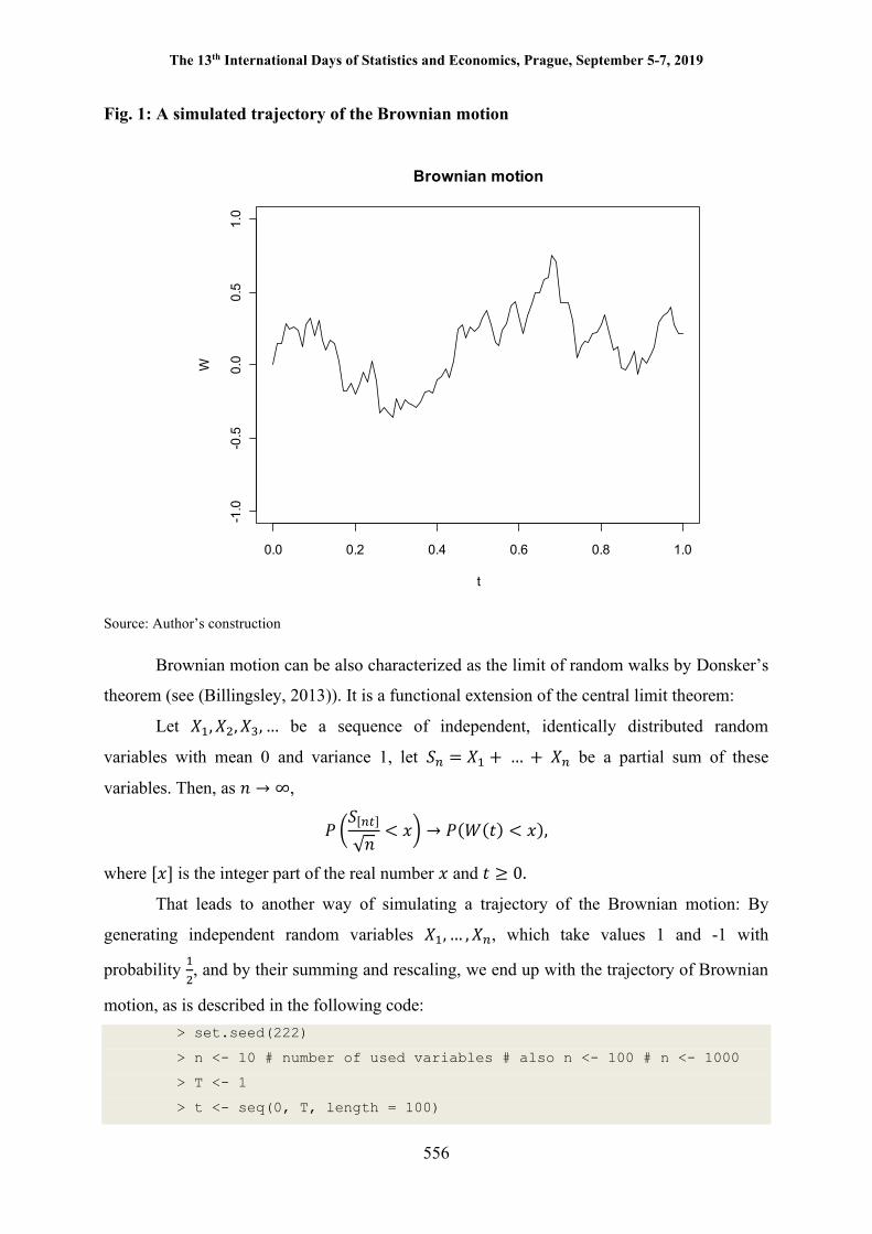
however due to the nature of R language, the second one is much faster. The simulated path of

the Brownian motion can be found in Figure 1.


556

Fig. 1: A simulated trajectory of the Brownian motion

Source: Author’s construction

Brownian motion can be also characterized as the limit of random walks by Donsker’s

theorem (see (Billingsley, 2013)). It is a functional extension of the central limit theorem:

Let 푋 , 푋 , 푋 , … be a sequence of independent, identically distributed random

variables with mean 0 and variance 1, let 푆 = 푋 + … + 푋 be a partial sum of these

variables. Then, as 푛 → ∞,

푃푆[ ]

√푛< 푥 → 푃(푊(푡) < 푥),

where [푥] is the integer part of the real number 푥 and 푡 ≥ 0.

That leads to another way of simulating a trajectory of the Brownian motion: By

generating independent random variables 푋 , … , 푋 , which take values 1 and -1 with

probability , and by their summing and rescaling, we end up with the trajectory of Brownian

motion, as is described in the following code: > set.seed(222)

> n <- 10 # number of used variables # also n <- 100 # n <- 1000

> T <- 1

> t <- seq(0, T, length = 100)

0.0 0.2 0.4 0.6 0.8 1.0

-1.0

-0.5

0.0

0.5

1.0

Brownian motion

t

W


557

> S <- cumsum(2*(runif(n) > 0.5) - 1)

> W <- sapply(t, function(x) ifelse(n*x > 0, S[n*x], 0))

> W <- as.numeric(W)/sqrt(n)

> plot(t, W, type = "l", main = "Brownian motion by random walks",

ylim = c(-1, 1))

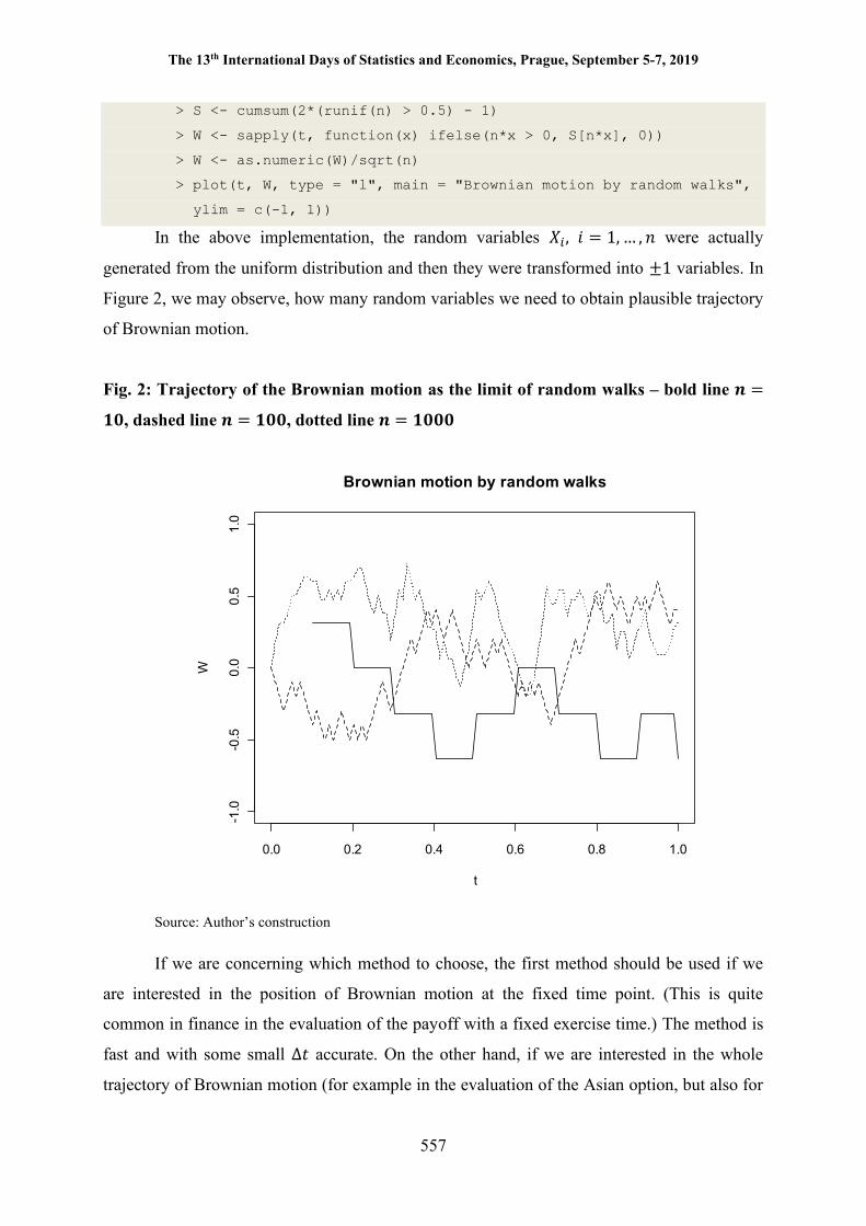
In the above implementation, the random variables 푋 , 푖 = 1, … , 푛 were actually

generated from the uniform distribution and then they were transformed into ±1 variables. In

Figure 2, we may observe, how many random variables we need to obtain plausible trajectory

of Brownian motion.

Fig. 2: Trajectory of the Brownian motion as the limit of random walks – bold line 풏 =

ퟏퟎ, dashed line 풏 = ퟏퟎퟎ, dotted line 풏 = ퟏퟎퟎퟎ


If we are concerning which method to choose, the first method should be used if we

are interested in the position of Brownian motion at the fixed time point. (This is quite

common in finance in the evaluation of the payoff with a fixed exercise time.) The method is

fast and with some small ∆푡 accurate. On the other hand, if we are interested in the whole

trajectory of Brownian motion (for example in the evaluation of the Asian option, but also for

0.0 0.2 0.4 0.6 0.8 1.0

-1.0

-0.5

0.0

0.5

1.0

Brownian motion by random walks

t

W


558

the description of the whole dynamic of the process), the second method (with some large

number of random variables 푛, e.g., 푛 ≥ 1000) could be used.

There are indeed many generalizations of Brownian motion, from which we mention

the shifted Brownian motion. Given a Brownian motion 푊(푡) and a point 푥 ∈ 푅, the process

푊 , (푡) = 푥 + 푊(푡), 푡 ≥ 0,

is a Brownian motion starting from the point 푥 instead of 0 at the time 0.

Furthermore, we may consider not only the shift in the space variable, but also the

shift in the time variable. If we want Brownian motion to start at some fixed time 푡 instead of

the time 0, we may define

푊 , (푡) = 푥 + 푊(푡) − 푊(푡 ), 푡 ≥ 푡 .

This is the process 푊 , = {푊(푡), 푡 ≤ 푡|푊(푡 ) = 푥}, i.e., it is the standard

Brownian motion conditioned in the way that 푊(푡 ) = 푥. Since the increments of Brownian

motion are independent on its past (which is called the Markov property, see (Stroock, 2013)),

the distribution of 푊 , (푡) and 푥 + 푊(푡 − 푡 ) are equal. Therefore the simulation of this

process starts with the simulation of Brownian motion, its shifting in the space (to the point 푥)

and then its translating in the time (so it starts at time 푡 ). (See the following Section for

similar construction.)

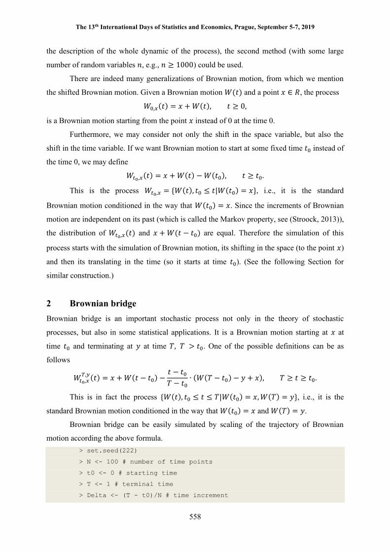
2 Brownian bridge Brownian bridge is an important stochastic process not only in the theory of stochastic

processes, but also in some statistical applications. It is a Brownian motion starting at 푥 at

time 푡 and terminating at 푦 at time 푇, 푇 > 푡 . One of the possible definitions can be as

follows

푊 ,, (푡) = 푥 + 푊(푡 − 푡 ) −

푡 − 푡푇 − 푡

∙ (푊(푇 − 푡 ) − 푦 + 푥), 푇 ≥ 푡 ≥ 푡 .

This is in fact the process {푊(푡), 푡 ≤ 푡 ≤ 푇|푊(푡 ) = 푥, 푊(푇) = 푦}, i.e., it is the

standard Brownian motion conditioned in the way that 푊(푡 ) = 푥 and 푊(푇) = 푦.

Brownian bridge can be easily simulated by scaling of the trajectory of Brownian

motion according the above formula. > set.seed(222)


> t0 <- 0 # starting time

> T <- 1 # terminal time

> Delta <- (T - t0)/N # time increment


559

> W <- numeric(N+1) # initialization of the vector W

> t <- seq(t0, T, length = N+1) # sequence of time points

> W <- c(0, cumsum(sqrt(Delta) * rnorm(N))) # Brownian motion

> x <- 1 # initial value

> y <- -1 # terminal value

> BB <- x + W - (t - t0)/(T - t0) * (W[N+1] - y + x)

> plot(t, BB, type = "l", main = "Brownian bridge")

Figure 3 shows simulated trajectory of the Brownian bridge starting from 푥 = 1 at

time 0 and terminating at 푦 = −1 at time 푇 = 1.

Fig. 3: A simulated trajectory of the Brownian bridge


3 Geometric Brownian motion Geometric Brownian motion is used to model stock prices in the Black–Scholes model and it

is the most widely used model of stock price behaviour (see (Black & Scholes, 1973)). The

process is continuous in time and it is the solution of the following so-called stochastic

differential equation

0.0 0.2 0.4 0.6 0.8 1.0

-1.0

-0.5

0.0

0.5

1.0

Brownian bridge

t

BB


560

푑푆(푡) = 휇푆(푡)푑푡 + 휎푆(푡)푑푊(푡), 푆(0) = 푥, 푡 ≥ 0. (1)

The motivation to the equation (1) is that the variation of the asset ∆푆 = 푆(푡 + ∆푡) −

푆(푡) in a small interval [푡, 푡 + ∆푡) has the following dynamics ∆푆푆

= 휇∆푡 + 휎∆푊. (2)

It means that the returns of the asset consist of some deterministic contribution, which

is dependent on the length of the interval ∆푡 (hence the term 휇∆푡) and some stochastic

contribution (randomness, noise, shocks, ...), which may behave independently and also

complying Gaussian distribution (hence the term 휎∆푊). Now if we multiply the equation (2)

by 푆 and let ∆푡 → 0, we arrive at (1).

However, to give a satisfactory meaning to the equation (1), we also have to introduce

its integral form

푆(푡) = 푆(0) + 휇 푆(푢)푑푢 + 휎 푆(푢)푑푊(푢) , 푡 ≥ 0. (3)

Since the variation of Brownian motion is not finite and its derivative nowhere exists

(see (Karatzas & Shreve, 1998)), there is a need to build a proper stochastic integration with

respect to the Brownian motion. It can be done (see also (Karatzas & Shreve, 1998)) and the

third term in (3) will obtain a rigorous meaning. The coefficient 휇 > 0 is interpreted as the

interest rate and the coefficient 휎 > 0 is interpreted as volatility. For more properties of the

geometric Brownian motion, see, e.g., (Ross, 2014).

The first way of simulating a trajectory of the geometric Brownian motion comes from

the equation (2). We divide the interval [0, 푇] equidistantly, and (starting from some positive

initial value 푆(0) = 푥 > 0) we generate the increments of the process {푆(푡), 푡 ≥ 0} according

the dynamics (2). This method is called the Euler’s method (see (Iacus, 2010)). set.seed(222)

N <- 100 # number of time points

T <- 1 # length of the interval [0,T]

x <- 5 # initial value

mu <- 1 # value of the parameter mu - rate

sigma <- 1 # value of the parameter sigma - volatility

Delta <- T/N # time increment

S <- numeric(N+1) # initialization of the vector S

S[1] <- x

W <- rnorm(N) # generation of increments of Brownian motion

for(i in 1:N)

S[i+1] <- S[i] + mu*S[i]*Delta + sigma*S[i]*sqrt(Delta)*W[i]


561

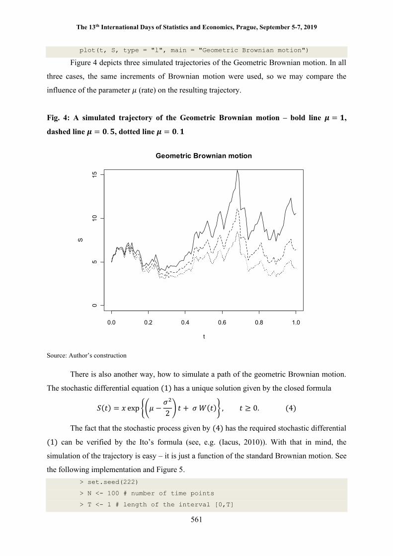
plot(t, S, type = "l", main = "Geometric Brownian motion")

Figure 4 depicts three simulated trajectories of the Geometric Brownian motion. In all

three cases, the same increments of Brownian motion were used, so we may compare the

influence of the parameter 휇 (rate) on the resulting trajectory.

Fig. 4: A simulated trajectory of the Geometric Brownian motion – bold line 흁 = ퟏ,

dashed line 흁 = ퟎ. ퟓ, dotted line 흁 = ퟎ. ퟏ


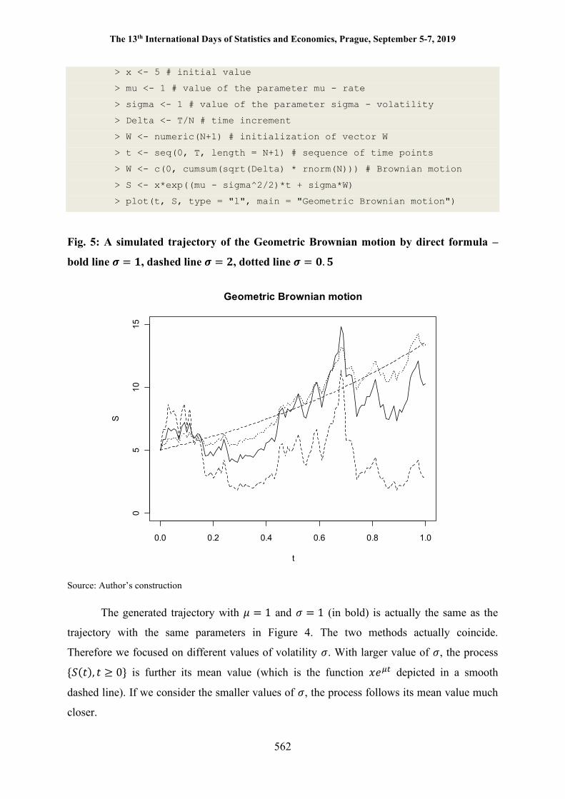
There is also another way, how to simulate a path of the geometric Brownian motion.

The stochastic differential equation (1) has a unique solution given by the closed formula

푆(푡) = 푥 exp 휇 −휎2

푡 + 휎 푊(푡) , 푡 ≥ 0. (4)

The fact that the stochastic process given by (4) has the required stochastic differential

(1) can be verified by the Ito’s formula (see, e.g. (Iacus, 2010)). With that in mind, the

simulation of the trajectory is easy – it is just a function of the standard Brownian motion. See

the following implementation and Figure 5. > set.seed(222)



0.0 0.2 0.4 0.6 0.8 1.0

05

1015

Geometric Brownian motion

t

S


562


> mu <- 1 # value of the parameter mu - rate

> sigma <- 1 # value of the parameter sigma - volatility


> W <- numeric(N+1) # initialization of vector W


> W <- c(0, cumsum(sqrt(Delta) * rnorm(N))) # Brownian motion

> S <- x*exp((mu - sigma^2/2)*t + sigma*W)

> plot(t, S, type = "l", main = "Geometric Brownian motion")

Fig. 5: A simulated trajectory of the Geometric Brownian motion by direct formula –

bold line 흈 = ퟏ, dashed line 흈 = ퟐ, dotted line 흈 = ퟎ. ퟓ


The generated trajectory with 휇 = 1 and 휎 = 1 (in bold) is actually the same as the

trajectory with the same parameters in Figure 4. The two methods actually coincide.

Therefore we focused on different values of volatility 휎. With larger value of 휎, the process

{푆(푡), 푡 ≥ 0} is further its mean value (which is the function 푥푒 depicted in a smooth

dashed line). If we consider the smaller values of 휎, the process follows its mean value much

closer.

0.0 0.2 0.4 0.6 0.8 1.0

05

1015

Geometric Brownian motion

t

S


563

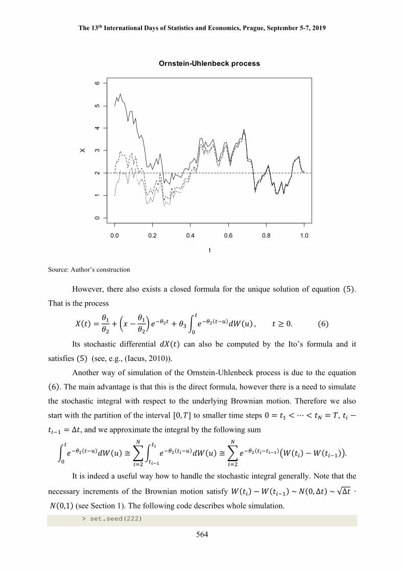
4 Ornstein-Uhlenbeck process Another stochastic process with applications both in financial mathematics and the physical

sciences is the Ornstein-Uhlenbeck process. The process is also continuous in time and it is

the solution of the following stochastic differential equation

푑푋(푡) = 휃 − 휃 푋(푡) 푑푡 + 휃 푑푊(푡), 푋(0) = 푥, 푡 ≥ 0, (5)

where 푥 ∈ 푅, 휃 , 휃 ∈ 푅 and 휃 > 0.

The model with 휃 = 0 was introduced by Ornstein and Uhlenbeck (see (Uhlenbeck &

Ornstein, 1930)) and with the reparametrization

푑푋(푡) = 휃 휇 − 푋(푡) 푑푡 + 휎 푑푊(푡), 푋(0) = 푥, 푡 ≥ 0,

is used in financial mathematics as Vasicek model (Vasicek, 1977). (Here 휇 is interpreted as

the long-run equilibrium of the process, 휃 as the speed of the reversion and 휎 as the

volatility.)

The simulation of the process follows the definition (5) and the Euler’s method is

implemented as follows. > set.seed(222)



> x <- 5 # initial value # also x <- 2 # x <- 1

> theta <- c(10, 5, 3.5) # values of the parameters


> X <- numeric(N+1) # initialization of vector X

> X[1] <- x


> W <- rnorm(N) # generating of increments of Brownian motion

> for(i in 1:N)

+ X[i+1] <- X[i] + (theta[1] - theta[2]*X[i]) * Delta +

+ theta[3] * sqrt(Delta) * W[i]

> plot(t, X, type = "l", main = "Ornstein-Uhlenbeck process")

Figure 6 shows three trajectories of the Ornstein-Uhlenbeck process, which differ in

initial value 푥, but they are all slowly attracted to the equilibrium state 휇 = 2.

Fig. 6: A simulated trajectory of the Ornstein-Uhlenbeck process – bold line 풙 = ퟓ,

dashed line 풙 = ퟐ, dotted line 풙 = ퟏ


564


However, there also exists a closed formula for the unique solution of equation (5).

That is the process

푋(푡) =휃휃

+ 푥 −휃휃

푒 + 휃 푒 ( )푑푊(푢) , 푡 ≥ 0. (6)

Its stochastic differential 푑푋(푡) can also be computed by the Ito’s formula and it

satisfies (5) (see, e.g., (Iacus, 2010)).

Another way of simulation of the Ornstein-Uhlenbeck process is due to the equation

(6). The main advantage is that this is the direct formula, however there is a need to simulate

the stochastic integral with respect to the underlying Brownian motion. Therefore we also

start with the partition of the interval [0, 푇] to smaller time steps 0 = 푡 < ⋯ < 푡 = 푇, 푡 −

푡 = ∆푡, and we approximate the integral by the following sum

푒 ( )푑푊(푢) ≅ 푒 ( )푑푊(푢) ≅ 푒 ( ) 푊(푡 ) − 푊(푡 ) .

It is indeed a useful way how to handle the stochastic integral generally. Note that the

necessary increments of the Brownian motion satisfy 푊(푡 ) − 푊(푡 ) ~ 푁(0, ∆푡) ~ √∆푡 ∙

푁(0,1) (see Section 1). The following code describes whole simulation. > set.seed(222)

0.0 0.2 0.4 0.6 0.8 1.0

01

23

45

6

Ornstein-Uhlenbeck process

t

X


565




> theta <- c(10, 5, 3.5) # values of the parameters


> X <- numeric(N+1) # initialization of vector X

> X[1] <- x


> stoch.integral <- c(0, sapply(2:(N+1), function (x){

+ exp(-theta[2]*(t[x] - t[x-1]))*sqrt(Delta)*rnorm(1)}))

> X <- sapply(1:(N+1), function(x){

+ theta[1]/theta[2]+(X[1]-theta[1]/theta[2])*exp(-theta[2]*t[x]) +

+ theta[3]*sum(stoch.integral[1:x])})

> plot(t, X, type = "l", main = "Ornstein-Uhlenbeck process")

Fig. 7: A simulated trajectory of the Ornstein-Uhlenbeck process by formula (ퟔ) – bold

line 휽ퟑ = ퟑ. ퟓ, dashed line 휽ퟑ = ퟏퟎ, dotted line 휽ퟑ = ퟏ


The bold line in Figure 7 is basically the same trajectory as the bold trajectory in

Figure 6 – these two methods again coincide. For now, we have chosen to keep the initial

0.0 0.2 0.4 0.6 0.8 1.0

02

46

810

Ornstein-Uhlenbeck process

t

X


566

value the same (푥 = 5) and we simulated three trajectories with different parameters of

volatility 휃 . All trajectories are approaching the equilibrium state 휇 = 2, but, again, the

larger volatility, the larger the variance of the process itself.

Conclusion We introduced the most important stochastic processes in theory of probability and

summarized some numerical methods and ideas on their simulation. We believe it is a useful

overview, because this topic is not paid too much attention to, and it should be helpful to

practitioners, programmers and students.

Acknowledgment This paper has been produced with contribution of long term institutional support of research

activities by Faculty of Informatics and Statistics, University of Economics, Prague.

References

Billingsley, P. (2013). Convergence of probability measures. New York: John Wiley & Sons.

Black, F., Scholes, M. (1973). The pricing of options and corporate liabilities. Journal of

political economy, 81(3), 637-654.

Cobb, L. (1981). Stochastic differential equations for the social sciences. Mathematical

Frontiers of the Social and Policy Sciences, 37-68.

Iacus, S. M. (2010). Simulation and inference for stochastic differential equations: With R

examples. New York, NY: Springer.

Kampen, N. V. (2007). Stochastic Processes. Stochastic Processes in Physics and Chemistry,

52-72.

Karatzas, I., Shreve, S. E. (1998). Brownian motion. In Brownian Motion and Stochastic

Calculus, 47-127.

Lions, J. – L., Temam, R., Wang, S. (1992). New formulations of the primitive equations of

atmosphere and applications. Nonlinearity, 5, 237-288.

Mayer-Brandis, T., Proske F. (2004). Explicit solution of a non-linear filtering problem for

Lévy processes with application to finance. Applied Mathematics and Optimization, 50, 119-

134.

Papanicolaou, G. C. (1995). Diffusion in Random Media. Surveys in Applied Mathematics,

205-253.


567

Ricciardi, L. M. (1977). Diffusion processes and related topics in Biology. Berlin: Springer-

Verlag.

Ross, S. M. (2014). Introduction to probability models. Academic Press.

Schoutens, W. (2003). Lévy processes in Finance: Pricing Financial Derivatives. Chichester:

Wiley.

Stroock, D. W. (2013). An introduction to Markov processes (Vol. 230). Springer Science &

Business Media.

Uhlenbeck, G. E., Ornstein, L. S. (1930). On the theory of the Brownian motion. Physical

review, 36(5), 823-841.

Vasicek, O. (1977). An equilibrium characterization of the term structure. Journal of financial

economics, 5(2), 177-188.

Contact

RNDr. Josef Janák, Ph.D.

University of Economics, Prague

Department of Mathematics

W. Churchill Sq. 1938/4, 13067 Prague 3

[email protected]

Documents

NUMERICAL ALGORITHMS FOR STOCHASTIC PROCESSES