Embed Size (px)
Citation preview
On the interaction of light with novel artificial materials –
Intriguing phenomena and an extended toolbox
Der Naturwissenschaftlichen
Fakultät
der Friedrich-Alexander-Universität
Erlangen-Nürnberg
zur
Erlangung des Doktorgrades Dr. rer.
nat.
vorgelegt von
Muhammad Abdullah Tariq Butt
aus Karatschi (Pakistan)
Als Dissertation genehmigt
von der Naturwissenschaftlichen Fakultät
der Friedrich-Alexander Universität Erlangen-
Nürnberg
Abgabe bei den Berichterstattern 11. 02 2021 Tag der mündlichen Prüfung 30. 03 2021 Vorsitzender des Promotionsorgans: Prof. Dr. Wolgang
Achtziger Gutachter: Prof. Dr. Gerd Leuchs Prof. Dr. Nicolas Joly

Beginning with the name of Almighty the most gracious, I dedicate
this thesis to my parents and better half, who have supported me
throughout my doctoral journey.

Abstract
This thesis summarizes the advantage and versatility of analyzing light-mater interaction
exploiting the polarization state of light. We use customized experimental systems to develop
specialized techniques to study intriguing optical phenomena at small scales for novel artificial
materials. The quintessential parts of this report are Chapter 3 and 4, which describe the
experimental results and analysis related to projects covered in this thesis.
In the first part of this thesis, we study the case of 3D novel self-assembled carbon flakes with
orthorhombic phase of carbon intercalated with bimetallic (Au-Ag) nanoclusters, fabricated from
liquid phase solution of a supra molecular complex (SMC) using laser induced deposition process.
The fabrication of carbon flakes was done by Prof. Alina Manshina and her group at St. Petersburg
State University, Russia. The challenge however, was the small lateral dimensions of individual
carbon flakes. Therefore, we developed a scheme (microscopic Müller matrix measurement
technique) to extract the optical properties of the carbon flakes, once the incoming and outgoing
polarization states of light are known. This technique combines the benefits of polarized light
matter interaction with the back focal plane (k-space / Fourier space) microscopy and the usage
of electrically controlled liquid crystals to perform a comprehensive polarization analysis in
transmission at small scales. With the help of experimental results and theoretical modelling
(performed by collaborators at University of Ottawa, Canada), we relate the optical birefringence
in the carbon flakes to the crystalline arrangement of carbon atoms in the orthorhombic lattice.
Later, we also study the dependence of optical and geometrical properties of carbon flakes on the
fabrication parameters. To access the direct information regarding refractive index of the carbon
flake, we implement a specialized single-shot ellipsometric technique with a resolution, in the
order of the wavelength. This provided us with a preliminary estimate of complex refractive
indices of carbon flake.
In the second part of this thesis, we focus on the concept of diffraction assisted chiral scattering
in 2D metasurfaces. By designing sub-wavelength scattering structures called meta-atoms and
periodically arranging them, metasurfaces can be realized with intriguing optical properties. By
finely selecting the shape, orientation, material, and size of meta-atoms, their optical response
can be tuned. When the meta-atoms are arranged with certain periodicity, it leads to the
generation of propagating surface modes, also known as surface lattice resonances (SLR).
Resultantly, a resonant coupling of incident light beam with individual meta-atom resonance and
grazing diffracted waves can occur. We discuss the in-plane scattering of individual meta-atom
and how it could be effectively coupled to the diffraction modes of a lattice to observe asymmetric
transmission in the far-fields. We elaborate this concept for a fourfold symmetric structure
(quadrumer). The simulations and fabrication were performed in collaboration with researchers
from Tecnologico de Monterrey, Mexico and University of Ottawa, Canada (also part of Max
Planck-University of Ottawa Centre for Extreme and Quantum Photonics), respectively. For
analysis of samples, we use an experimental setup to angularly resolve transmitted light to study
asymmetric transmission in zeroth and first diffraction orders. For our case of a fourfold
symmetric quadrumer, an in-plane rotation of each quadrumer by 22.5°/-22.5° leads to
asymmetric transmission in first diffraction order. The zeroth order does not exhibit any
asymmetry. We analyze simulation and experimental results and find them in good agreement.

In the outlook chapter of this thesis, we discuss future works related to localized modification of
carbon flakes and extension of our ellipsometric scheme using polarization tailored light beams.
We also elaborate on few designs/ideas for observing asymmetric transmission in symmetric
structures as a future extension of our present work.
Zusammenfassung
Diese Arbeit beschäftigt sich mit den Vorteilen und der Vielseitigkeit der Analyse von Licht-
Materie-Wechselwirkung unter Ausnutzung des Polarisationszustands des Lichts. Wir verwenden
maßgeschneiderte experimentelle Systeme, zur Entwicklung spezieller Techniken für die
Untersuchung faszinierender optischer Phänomene auf kleinen Längenskalen in Bezug auf
neuartige künstliche Materialien. Der wesentliche Teil dieses Berichts sind die Kapitel 3 und 4, in
denen die experimentellen Ergebnisse und Analysen der in dieser Arbeit behandelten Projekte
beschrieben werden.
Im ersten Teil dieser Arbeit untersuchen wir 3D neuartige selbstorganisierter Kohlenstoffflocken
mit orthorhombischer Kohlenstoffphase, die mit bimetallischen (Au-Ag) -Nanoclustern
interkaliert sind und aus einer Flüssigphasenlösung eines supra-molekularen Komplexes (SMC)
unter Verwendung eines laserinduzierten Abscheidungsprozesseshergestellt wurden. Die
Herstellung von Kohlenstoffflocken wurde von Prof. Alina Manshina und ihrer Gruppe an der
staatlichen Universität St. Petersburg in Russland durchgeführt. Die Herausforderung sind jedoch
die geringen seitlichen Abmessungen der einzelnen Kohlenstoffflocken. Daher haben wir ein
System (mikroskopische Müller-Matrix-Messtechnik) entwickelt, um die optischen Eigenschaften
der Kohlenstoffflocken zu extrahieren, sobald die ein- und ausgehenden Polarisationszustände
des Lichts bekannt sind. Diese Technik kombiniert die Vorteile polarisierter Licht-Materie-
Wechselwirkung mit der Mikroskopie der hinteren Brennebene (k-Raum / Fourier-Raum) und der
Verwendung elektrisch gesteuerter Flüssigkristalle, um eine umfassende Polarisationsanalyse in
Transmission auf kleinen Größenskalen durchzuführen. Mit Hilfe experimenteller Ergebnisse und
theoretischer Modelle (durchgeführt von unseren Partnern an der Universität von Ottawa,
Kanada) beziehen wir die optische Doppelbrechung in den Kohlenstoffflocken auf die kristalline
Anordnung von Kohlenstoffatomen im orthorhombischen Gitter. Später untersuchen wir auch die
Abhängigkeit der optischen und geometrischen Eigenschaften von Kohlenstoffflocken von den
Herstellungsparametern. Um auf die direkten Informationen bezüglich des Brechungsindex der
Kohlenstoffflocke zugreifen zu können, wurde eine spezielle Einzelbild ellipsometrische Technik
mit einer Auflösung in der Größenordnung der Wellenlänge implementiert. Dies liefert uns eine
vorläufige Abschätzung der komplexen Brechungsindizes der Kohlenstoffflocken.
Im zweiten Teil dieser Arbeit konzentrieren wir uns auf das Verständnis der
beugungsunterstützten chiralen Streuung in 2D-Metaoberflächen. Indem wir Sub-Wellenlängen-
Streustrukturen, sogenannte Meta-atome, entwerfen und periodisch anordnen, können wir
Metaoberflächen mit verblüffenden optischen Eigenschaften realisieren. Durch genaue Auswahl
von Form, Ausrichtung, Material und Größe der Meta-atome können wir deren Reaktion auf
optische Anregung einstellen. Wenn die Meta-atome mit einer bestimmten Periodizität
angeordnet sind, führt dies zur Erzeugung von sich ausbreitenden Oberflächenmoden, die auch
als Oberflächengitterresonanzen (SLR) bezeichnet werden. Infolgedessen kann eine resonante
Kopplungdes einfallenden Lichtstrahls an eine individuelle Meta-atom-Resonanz und streifenden
gebeugten Wellen auftreten. Wir werden die Streuung einzelner Meta-atome in der Ebene
diskutieren und wie sie effektiv an die Beugungsmoden eines Gitters gekoppelt werden kann, um
eine asymmetrische Transmission im Fernfeld zu beobachten. Wir werden dieses Konzept für eine
vierfach symmetrische Struktur (Quadrumer) ausarbeiten.
Die Simulationen und die Herstellung wurden in Zusammenarbeit mit Forschern des Tecnologico
de Monterrey, Mexico, und der Universität von Ottawa, Kanada (ebenfalls Teil des Zentrums für
Extreme und Quantenphotonik der Max-Planck-Universität von Ottawa) durchgeführt. Zur
Analyse von Proben verwenden wir einen Versuchsaufbau, welcher eine Winkel-aufgelöste
Messung des transmittierten Lichts erlaubt, um die asymmetrische Transmission in nullter und
erster Beugungsordnung zu untersuchen. Für den vorliegenden Fall eines vierfach symmetrischen
Quadrumers führt eine Drehung jedes Quadrumers in der Ebene um 22,5 ° / -22,5 ° zu einer
asymmetrischen Transmission in der ersten Beugungsordnung. Die nullte Ordnung zeigt keine
Asymmetrie. Simulations- und Versuchsergebnisse weisen eine gute Übereinstimmung auf.
Im Ausblick-Kapitel dieser Arbeit diskutieren wir zukünftige Projekte zur lokalisierten Modifikation
von Kohlenstoffflocken und zur Erweiterung unseres ellipsometrischen Schemas mithilfe speziell
polarisierter Lichtstrahlen. Wir arbeiten außerdem einige Designs/ideen von Meta-atomen zur
Beobachtung der asymmetrischen Transmission in symmetrischen Strukturen als zukünftige
Erweiterung unserer gegenwärtigen Arbeit aus.
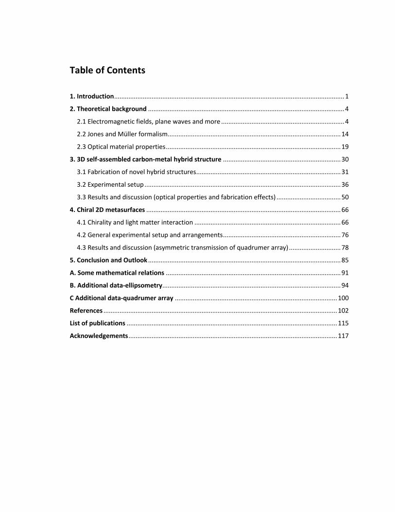
Table of Contents
1. Introduction ................................................................................................................................. 1
2. Theoretical background .............................................................................................................. 4
2.1 Electromagnetic fields, plane waves and more ..................................................................... 4
2.2 Jones and Müller formalism ................................................................................................. 14
2.3 Optical material properties .................................................................................................. 19
3. 3D self-assembled carbon-metal hybrid structure .................................................................. 30
3.1 Fabrication of novel hybrid structures ................................................................................. 31
3.2 Experimental setup .............................................................................................................. 36
3.3 Results and discussion (optical properties and fabrication effects) .................................... 50
4. Chiral 2D metasurfaces ............................................................................................................. 66
4.1 Chirality and light matter interaction .................................................................................. 66
4.2 General experimental setup and arrangements .................................................................. 76
4.3 Results and discussion (asymmetric transmission of quadrumer array) ............................. 78
5. Conclusion and Outlook ............................................................................................................ 85
A. Some mathematical relations .................................................................................................. 91
B. Additional data-ellipsometry .................................................................................................... 94
C Additional data-quadrumer array ........................................................................................... 100
References ................................................................................................................................... 102
List of publications ...................................................................................................................... 115
Acknowledgements ..................................................................................................................... 117

1. Introduction
In the last decade, miniaturization of electronic devices has pushed the field of nanotechnology
to define the new boundaries of science [1-6]. Nano-optics, a related field, deals with the
interaction of light with matter at nanoscale [7-9]. In this thesis, we demonstrate the advantage
and versatility of analyzing light-mater interaction, exploiting polarization state of light. We used
customized in-home built experimental systems [10-13] to devise ways and methods to study
intriguing optical phenomena at small scales. Most of the studies were performed in collaboration
with scientists across the globe belonging from different fields of science [14-20].
To begin our journey, initially we will consider the theoretical foundations related to the light
matter interaction in Chapter 2 of this thesis. We will discuss the polarization state of light and
how it alters when interacting with matter. This understanding will later help us to study the
inverse case. To extract the optical properties of a medium, once the incoming and outgoing
polarization states of light are known. Although being developed and used for over a century,
polarimetric analysis methods have evolved over time. Nanotechnology has provided room for
newer miniaturized devices, sophisticated analysis techniques to find their applications in
characterizing materials and structures with unprecedented accuracy and scales.
A similar case in hand, was of 3D novel self-assembled orthorhombic phase of carbon intercalated
with bimetallic (Au-Ag) nanoclusters, fabricated from liquid phase solution of a supra molecular
complex (SMC) by laser induced deposition process. The fabrication was done by Professor Alina
Manshina and her group at St. Petersburg State University, Russia [20-24]. The structure manifests
itself in the form of cuboid (called caron flake) with lateral dimensions of a few microns and
thickness of a few hundred nanometers. Due to its organo-metallic composition, it finds
application in plasmonic sensing platforms [25, 26] with future prospects of being used for light
guiding and plasmonics applications. We will discuss details about carbon flakes fabrication and
structure briefly in the first section of Chapter 3. The case, as intriguing, forced us to look and
think deeply in understanding the nature of this complex structure. Initial studies performed at
Max Planck institute for the science of light pointed towards interesting optical properties related
to carbon flake. Therefore, it was decided to perform a complete investigation into the optical
properties. The challenge however, was the small lateral dimensions of individual carbon flakes.
The commercially available polarimetric and ellipsometric setups usually provide resolution of
tens of microns which would not be helpful in our case.
Henceforth, an in-house built experimental setup [10-13, 27, 28] (previously used to study to
nanostructures) was modified to perform the polarimetric analysis of carbon flakes. The
microscopic Müller matrix measurement technique, as we call it, merges the benefits of polarized
light matter interaction with the back focal plane (k-space / Fourier space) microscopy [29] and
the usage of liquid crystal variable retarders (LCVRs) to perform a comprehensive polarization
analysis in transmission at small scales [14, 18, 30, 31].
The theoretical concepts related to this technique will already be discussed in Chapter 2, while
the experimental setup, its peculiarities and working behavior will be discussed in Chapter 3. We
1. Introduction
2
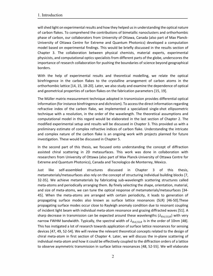
will shed light on experimental results and how they helped us in understanding the optical nature
of carbon flakes. To comprehend the contributions of bimetallic nanoclusters and orthorhombic
phase of carbon, our collaborators from University of Ottawa, Canada (also part of Max Planck-
University of Ottawa Centre for Extreme and Quantum Photonics) developed a computation
model based on experimental findings. This would be briefly discussed in the results section of
Chapter 3. The collaboration between physical chemists, material experts, experimental
physicists, and computational optics specialists from different parts of the globe, underscores the
importance of research collaboration for pushing the boundaries of science beyond geographical
borders.
With the help of experimental results and theoretical modelling, we relate the optical
birefringence in the carbon flakes to the crystalline arrangement of carbon atoms in the
orthorhombic lattice [14, 15, 18-20]. Later, we also study and examine the dependence of optical
and geometrical properties of carbon flakes on the fabrication parameters [15, 19].
The Müller matrix measurement technique adopted in transmission provides differential optical
information (for instance birefringence and dichroism). To access the direct information regarding
refractive index of the carbon flake, we implemented a specialized single-shot ellipsometric
technique with a resolution, in the order of the wavelength. The theoretical assumptions and
computational model in this regard would be elaborated in the last section of Chapter 2. The
modified experimental setup and results will be discussed in Chapter 3. This provided us with a
preliminary estimate of complex refractive indices of carbon flake. Understanding the intricate
and complex nature of the carbon flake is an ongoing work with projects planned for future
investigation. These would be discussed in Chapter 5.
In the second part of this thesis, we focused onto understanding the concept of diffraction
assisted chiral scattering in 2D metasurfaces. This work was done in collaboration with
researchers from University of Ottawa (also part of Max Planck-University of Ottawa Centre for
Extreme and Quantum Photonics), Canada and Tecnologico de Monterrey, Mexico.
Just like self-assembled structures discussed in Chapter 3 of this thesis,
metamaterials/metasurfaces also rely on the concept of structuring individual building blocks [7,
32-35]. We achieve metamaterials by fabricating sub-wavelength scattering structures called
meta-atoms and periodically arranging them. By finely selecting the shape, orientation, material,
and size of meta-atoms, we can tune the optical response of metamaterials/metasurfaces [34-
45]. When the meta-atoms are arranged with certain periodicity, it leads to generation of
propagating surface modes also known as surface lattice resonances (SLR) [46-50].These
propagating surface modes occur close to Rayleigh anomaly condition due to resonant coupling
of incident light beam with individual meta-atom resonance and grazing diffracted waves [51]. A
sharp decrease in transmission can be expected around these wavelengths (𝜆𝑅𝐴/𝑆𝐿𝑅) with very
narrow FWHM bandwidth. Typically, the spectral width of 𝜆𝑅𝐴/𝑆𝐿𝑅 is in the order of 10nm [48].
This has instigated a lot of research towards application of surface lattice resonances for sensing
devices [47, 49, 52-54]. We will review the relevant theoretical concepts related to the design of
chiral meta-atom in first section of Chapter 4. Later, we will discuss the in-plane scattering of
individual meta-atom and how it could be effectively coupled to the diffraction orders of a lattice
to observe asymmetric transmission in surface lattice resonances [48, 52-55]. We will elaborate
1. Introduction
3
this concept for a fourfold symmetric structure (quadrumer). Using, Finite difference time domain
(FDTD) simulation, we found out that for a chiral orientation ( in-plane rotation of 22.5°/-22.5°) at
certain periodicity (600nm) leads to asymmetric transmission in first diffraction order. This does
not happen for symmetric orientation (0° and 45° in-plane rotation). Besides this, due to
symmetry reasons, the zeroth order does not exhibit any asymmetric transmission. The
simulations were performed by research collaborators from Tecnologico de Monterrey, Mexico.
Later, the fabrication of requisite samples was done at University of Ottawa, Canada. For analysis
of samples, we use an experimental setup to angularly resolve transmitted light to study
asymmetric transmission in zeroth and first diffraction orders. We analyze simulation and
experimental results in last section of Chapter 4, which are found to be in good agreement.
In outlook chapter of this thesis, we elaborate on few designs of meta-atom for observing
asymmetric transmission in rotationally symmetric structures as future extension of our present
work.
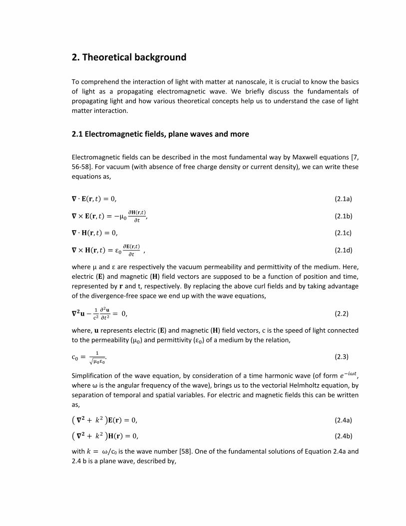
2. Theoretical background
To comprehend the interaction of light with matter at nanoscale, it is crucial to know the basics
of light as a propagating electromagnetic wave. We briefly discuss the fundamentals of
propagating light and how various theoretical concepts help us to understand the case of light
matter interaction.
2.1 Electromagnetic fields, plane waves and more
Electromagnetic fields can be described in the most fundamental way by Maxwell equations [7,
56-58]. For vacuum (with absence of free charge density or current density), we can write these
equations as,
𝛁 ∙ 𝐄(𝐫, 𝑡) = 0, (2.1a)
𝛁 × 𝐄(𝐫, 𝑡) = −μ0∂𝐇(𝐫,𝑡)
∂𝑡, (2.1b)
𝛁 ∙ 𝐇(𝐫, 𝑡) = 0, (2.1c)
𝛁 × 𝐇(𝐫, 𝑡) = ε0∂𝐄(𝐫,𝑡)
∂𝑡 , (2.1d)
where μ and ε are respectively the vacuum permeability and permittivity of the medium. Here,
electric (𝐄) and magnetic (𝐇) field vectors are supposed to be a function of position and time,
represented by 𝐫 and t, respectively. By replacing the above curl fields and by taking advantage
of the divergence-free space we end up with the wave equations,
𝛁𝟐𝐮 −1
c2
∂2𝐮
∂𝑡2 = 0, (2.2)
where, 𝐮 represents electric (𝐄) and magnetic (𝐇) field vectors, c is the speed of light connected
to the permeability (μ0) and permittivity (ε0) of a medium by the relation,
c0 = 1
√μ0ε0. (2.3)
Simplification of the wave equation, by consideration of a time harmonic wave (of form 𝑒−𝑖𝜔𝑡,
where ω is the angular frequency of the wave), brings us to the vectorial Helmholtz equation, by
separation of temporal and spatial variables. For electric and magnetic fields this can be written
as,
( 𝛁𝟐 + 𝑘2 )𝐄(𝐫) = 0, (2.4a)
( 𝛁𝟐 + 𝑘2 )𝐇(𝐫) = 0, (2.4b)
with 𝑘 = ω/c0 is the wave number [58]. One of the fundamental solutions of Equation 2.4a and
2.4 b is a plane wave, described by,
2. Theoretical background
5
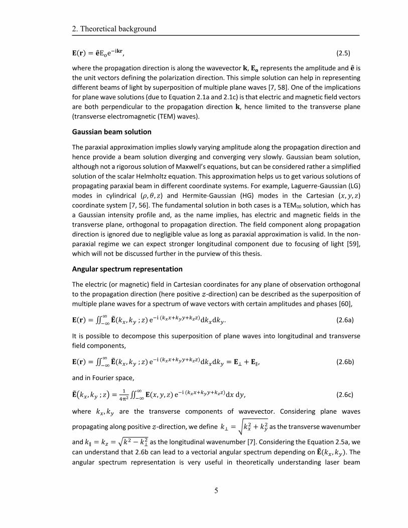
𝐄(𝐫) = ��Eoe−i𝐤𝐫, (2.5)
where the propagation direction is along the wavevector 𝐤, 𝐄𝐨 represents the amplitude and �� is
the unit vectors defining the polarization direction. This simple solution can help in representing
different beams of light by superposition of multiple plane waves [7, 58]. One of the implications
for plane wave solutions (due to Equation 2.1a and 2.1c) is that electric and magnetic field vectors
are both perpendicular to the propagation direction 𝐤, hence limited to the transverse plane
(transverse electromagnetic (TEM) waves).
Gaussian beam solution
The paraxial approximation implies slowly varying amplitude along the propagation direction and
hence provide a beam solution diverging and converging very slowly. Gaussian beam solution,
although not a rigorous solution of Maxwell’s equations, but can be considered rather a simplified
solution of the scalar Helmholtz equation. This approximation helps us to get various solutions of
propagating paraxial beam in different coordinate systems. For example, Laguerre-Gaussian (LG)
modes in cylindrical (𝜌, 𝜃, 𝑧) and Hermite-Gaussian (HG) modes in the Cartesian (𝑥, 𝑦, 𝑧)
coordinate system [7, 56]. The fundamental solution in both cases is a TEM00 solution, which has
a Gaussian intensity profile and, as the name implies, has electric and magnetic fields in the
transverse plane, orthogonal to propagation direction. The field component along propagation
direction is ignored due to negligible value as long as paraxial approximation is valid. In the non-
paraxial regime we can expect stronger longitudinal component due to focusing of light [59],
which will not be discussed further in the purview of this thesis.
Angular spectrum representation
The electric (or magnetic) field in Cartesian coordinates for any plane of observation orthogonal
to the propagation direction (here positive 𝓏-direction) can be described as the superposition of
multiple plane waves for a spectrum of wave vectors with certain amplitudes and phases [60],
𝐄(𝐫) = ∬ ��(𝑘𝑥 , 𝑘𝑦 ; 𝑧)∞
−∞e−i (𝑘𝑥𝑥+𝑘𝑦𝑦+𝑘𝑧𝑧)d𝑘𝑥d𝑘𝑦. (2.6a)
It is possible to decompose this superposition of plane waves into longitudinal and transverse
field components,
𝐄(𝐫) = ∬ ��(𝑘𝑥 , 𝑘𝑦 ; 𝑧)∞
−∞e−i (𝑘𝑥𝑥+𝑘𝑦𝑦+𝑘𝑧𝑧)d𝑘𝑥d𝑘𝑦 = 𝐄⊥ + 𝐄∥, (2.6b)
and in Fourier space,
��(𝑘𝑥 , 𝑘𝑦 ; 𝑧) =1
4π2 ∬ 𝐄(𝑥, 𝑦, 𝑧)∞
−∞e−i (𝑘𝑥𝑥+𝑘𝑦𝑦+𝑘𝑧𝑧)d𝑥 d𝑦, (2.6c)
where 𝑘𝑥, 𝑘𝑦 are the transverse components of wavevector. Considering plane waves
propagating along positive 𝓏-direction, we define 𝑘⊥ = √𝑘𝑥2 + 𝑘𝑦
2 as the transverse wavenumber
and 𝑘∥ = 𝑘𝑧 = √𝑘2 − 𝑘⊥2 as the longitudinal wavenumber [7]. Considering the Equation 2.5a, we
can understand that 2.6b can lead to a vectorial angular spectrum depending on ��(𝑘𝑥 , 𝑘𝑦). The
angular spectrum representation is very useful in theoretically understanding laser beam
2. Theoretical background
6
propagation and focusing of light waves. Moreover, considering 2.6c, the Fourier transformed
field evolves along the propagation direction in the following way,
𝐄(𝑘𝑥, 𝑘𝑦 ; 𝑧) = 𝐄(𝑘𝑥, 𝑘𝑦 ; 0)e±i𝑘𝑧𝑧, (2.7)
where the ± sign depends on the direction of propagation (+ for 𝓏 > 0 propagation direction). This
means that in reciprocal (angular spectrum) space, the field at any point along 𝓏 is equal to the
field at object plane (𝓏 = 0) times the propagator e±ikzz. Using this assumption, Equation 2.6a
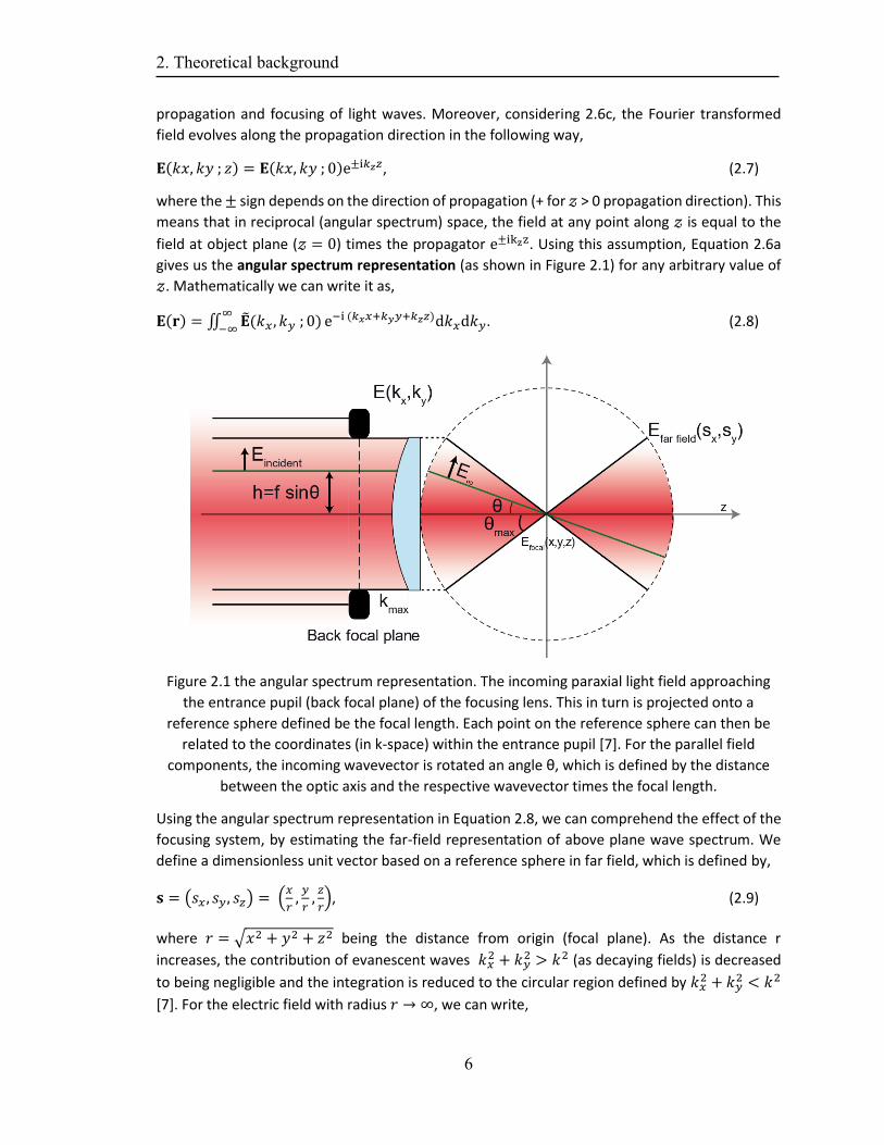
gives us the angular spectrum representation (as shown in Figure 2.1) for any arbitrary value of
𝓏. Mathematically we can write it as,
𝐄(𝐫) = ∬ ��(𝑘𝑥 , 𝑘𝑦 ; 0)∞
−∞e−i (𝑘𝑥𝑥+𝑘𝑦𝑦+𝑘𝑧𝑧)d𝑘𝑥d𝑘𝑦. (2.8)
Figure 2.1 the angular spectrum representation. The incoming paraxial light field approaching
the entrance pupil (back focal plane) of the focusing lens. This in turn is projected onto a
reference sphere defined be the focal length. Each point on the reference sphere can then be
related to the coordinates (in k-space) within the entrance pupil [7]. For the parallel field
components, the incoming wavevector is rotated an angle θ, which is defined by the distance
between the optic axis and the respective wavevector times the focal length.
Using the angular spectrum representation in Equation 2.8, we can comprehend the effect of the
focusing system, by estimating the far-field representation of above plane wave spectrum. We
define a dimensionless unit vector based on a reference sphere in far field, which is defined by,
𝐬 = (𝑠𝑥 , 𝑠𝑦, 𝑠𝑧) = (𝑥
𝑟,𝑦
𝑟,𝑧
𝑟), (2.9)
where 𝑟 = √𝑥2 + 𝑦2 + 𝑧2 being the distance from origin (focal plane). As the distance r
increases, the contribution of evanescent waves 𝑘𝑥2 + 𝑘𝑦
2 > 𝑘2 (as decaying fields) is decreased
to being negligible and the integration is reduced to the circular region defined by 𝑘𝑥2 + 𝑘𝑦
2 < 𝑘2
[7]. For the electric field with radius 𝑟 → ∞, we can write,

2. Theoretical background
7
𝑬∞(𝑠𝑥 , 𝑠𝑦, 𝑠𝑧) = lim𝑘𝑟→∞
∬ 𝑬(𝑘𝑥, 𝑘𝑦 ; 0)𝑒−𝑖𝑘𝑟(𝑘𝑥𝑘
𝑠𝑥+𝑘𝑦
𝑘𝑠𝑦+
𝑘𝑧𝑘
𝑠𝑧)d𝑘𝑥d𝑘𝑦𝑘⊥2 ≤ 𝑘2 . (2.10)
We solve the integral by applying the method for stationary phase [61]. This helps us to link the
far field reference sphere to initial field by relation,
𝐬 = (𝑠𝑥 , 𝑠𝑦, 𝑠𝑧) =𝑘𝑥
𝑘+
𝑘𝑦
𝑘+
𝑘𝑧
𝑘 (2.11)
This implies that, only a single incident plane wave out of plane wave spectrum defined by a wave
vector 𝐤 = (𝑘𝑥, 𝑘𝑦, 𝑘𝑧), contributes to a point on the reference sphere 𝐬 = (𝑠𝑥 , 𝑠𝑦, 𝑠𝑧). This
happens because rapidly oscillating phase terms in the integral in Equation 2.8 add up
destructively except the slowly varying phase corresponding to a certain wavevector contribute
significantly as defined in Equation 2.9. Hence, due to this elegant mathematical relation, we can
link the incident field in k-space to the far field of a focusing system.
𝑬(𝑘𝑥 , 𝑘𝑦; 0) = 𝑖𝑟
2𝜋
𝑒−𝑖𝑘𝑟
𝑘𝑧𝑬∞(𝑠𝑥 , 𝑠𝑦). (2.12)
This mathematical concept can be utilized to understand focusing of various types of light beams
and also for studying the inverse problem; to extract the response of a system in focal plane by
evaluating far field angular spectrum. This will also be of prime importance in the discussion of
experimental setups in the next chapters, where the angular spectrum of a collection microscope
objective is imaged to extract optical properties of an examined system [14, 15, 56, 62].
Polarization states of light
As shown in Equation 2.5a, a polarized light field can always be written as superposition of two
orthogonal plane waves. This could be performed in various coordinate systems [7, 63, 64]. For
two orthogonal plane waves polarized along 𝑥 and 𝑦 direction in a cartesian coordinate system
propagating along positive 𝑧-direction [65] we have
𝐄1 = 𝐄x + 𝐄y (2.13a)
𝐄x = E𝑥0��e−i (𝑤𝑡−k𝑧)eiδx, (2.13b)
𝐄y = E𝑦0��e−i (𝑤𝑡−k𝑧)eiδy and (2.13c)
We can define spatially homogenous incident light beam into three polarization types namely
linear, circular, and elliptical polarized light [7, 56, 58, 64]. We make the distinction based on the
individual amplitudes and relative phase difference (Δ δ = δx − δy) between the two constituent
orthogonal plane waves. The polarization state of light can be visualized and described in different
ways. For example, using the polarization ellipse (shown in Figure 2.2) in which, for all positions
along propagation direction (z-axis), we observe the fields in time in the 𝑥𝑦-plane. The two
defining parameters (as shown in Figure 2.2) in plotting a polarization ellipse are azimuthal angle
(θ ranging from −π
2−
π
2 ) and ellipticity angle (φ ranging from
−π
4−
π
4 ).
2. Theoretical background
8
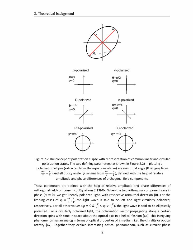
Figure 2.2 The concept of polarization ellipse with representation of common linear and circular
polarization states. The two defining parameters (as shown in Figure 2.2) in plotting a
polarization ellipse (extracted from the equations above) are azimuthal angle (θ ranging from −𝜋
2−
𝜋
2 ) and ellipticity angle (𝜑 ranging from
−𝜋
4−
𝜋
4 ), defined with the help of relative
amplitude and phase differences of orthogonal field components.
These parameters are defined with the help of relative amplitude and phase differences of
orthogonal field components of Equations 2.13b&c. When the two orthogonal components are in
phase (φ = 0), we get linearly polarized light, with respective azimuthal direction (θ). For the
limiting cases of φ =−π
4,π
4, the light wave is said to be left and right circularly polarized,
respectively. For all other values (φ ≠ 0 &−π
4< φ >
−π
4), the light wave is said to be elliptically
polarized. For a circularly polarized light, the polarization vector propagating along a certain
direction spins with time in space about the optical axis in a helical fashion [66]. This intriguing
phenomenon has an analog in terms of optical properties of a medium, i.e., the chirality or optical
activity [67]. Together they explain interesting optical phenomenon, such as circular phase
2. Theoretical background
9
retardation [68] and differential extinction [69] in a medium. These would be discussed in later
part of this thesis.
Boundary conditions and Fresnel equations
Next, we discuss boundary conditions based on polarized light interaction with an interface using
Maxwell’s equations. The incident (𝑬1), transmitted (𝑬2) and reflected (𝑬𝑟1) fields can then be
further evaluated using Fresnel equations [66, 70]. Based on the conservation of energy, the
vectors mentioned above can be written as,
|𝐄1|2 = |𝐄2|
2 + |𝐄r1|2, (2.14a)
and for Fresnel complex amplitude reflection/transmission coefficient can be related as [66, 70],
𝐄2r1⁄
TETM⁄
= c2/r1
TETM⁄
. 𝐄1
TETM⁄
, (2.14b)
where, 𝑐2/𝑟1
𝑇𝐸𝑇𝑀⁄
defines the respective complex amplitude coefficients between medium 1 & 2 [58,
65, 70]. We consider an interface between two mediums with different refractive index (n1 & n2).
The Maxwell curl and divergence equations (refer Equation 2.1a-d) leads us to the boundary
condition for the tangential electric field and normal displacement field components respectively
being continuous and mathematically shown as,
𝐄∥1 = 𝐄∥
2, 𝐃⊥1 = 𝐃⊥
2 , (2.15a)
where 𝑫 = 휀𝑟𝜖0𝑬, and 휀𝑟 being relative permittvity of the medium. In a similar fashion we can
derive the boundary condition for magnetic fields. Here, for ease of mathematical process, we
define orthogonal plane waves as parallel and perpendicular to the plane of incidence as shown
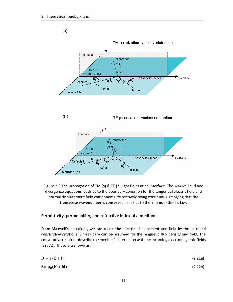
in Figure 2.3. These are mathematically defined as [7],
𝐄1 = 𝐄TM1 + 𝐄TE
1 , (2.15b)
where 𝐸𝑇𝑀1 is parallel and 𝐸𝑇𝐸
1 is perpendicular (senkrecht) to the plane of incidence as shown in
Figure 2.3. We consider the interface between two mediums as shown in Figure 2.3 with refractive
indices, permittivity and permeability referred to as n1, ε1, μ1 and n2, ε2, μ2 for medium 1 and 2
respectively. In a similar fashion, for incident and transmitted beam we can define the wavevector
considering boundary conditions as,
𝐤1 = (𝑘𝑥1, 𝑘𝑦1, 𝑘𝑧1), |𝐤1| = 𝑘1 = ω
c √ε1μ1, (2.16a)
𝐤2 = (𝑘𝑥2, 𝑘𝑦2, 𝑘𝑧2), |𝐤2| = 𝑘2 = ω
c √ε2μ2, (2.16b)
Here, the definition of transverse and longitudinal wavenumber are the same as mentioned above
for Equation 2.6c. From the boundary conditions in Equation 2.15 we can also deduce that,
𝑘𝑥1 = 𝑘𝑥2 = 𝑘𝑥 , 𝑘𝑦1 = 𝑘𝑦2 = 𝑘𝑦 and (2.17a)
2. Theoretical background
10
|𝐤1| = |𝐤0|n1. (2.17b)
Implying that transverse wavenumber is conserved. In fact, this leads us also to the infamous
Snell’s law [58]. Considering the incident wavevector 𝐤1 making an angle of 𝜃 with the normal to
the interface (as shown in Figure 2.2) [7], we can define the component parallel to the interface
by,
k∥1 = |𝑘1| sin θ1 = k∥2 = |𝑘2| sin θ2 = √𝑘𝑥2 + 𝑘𝑦
2, (2.18a)
and for the longitudinal wavevector component we can write,
𝑘𝑧1 = 𝑘⊥1 = |k1| cos θ1 = √𝑘12 − 𝑘∥
2, (2.18b)
𝑘𝑧2 = 𝑘⊥2 = |k2| cos θ2 = √𝑘22 − 𝑘∥
2. (2.18c)
Considering the above-mentioned equations, we can now deduce the case for transmitted and
reflected fields at an interface by applying boundary conditions for electric and magnetic fields
and analytically solving them. For a linear homogeneous isotropic medium, the electric and
magnetic fields are related by intrinsic impedance 𝑧 = √μ
ɛ of the medium and thus we end up
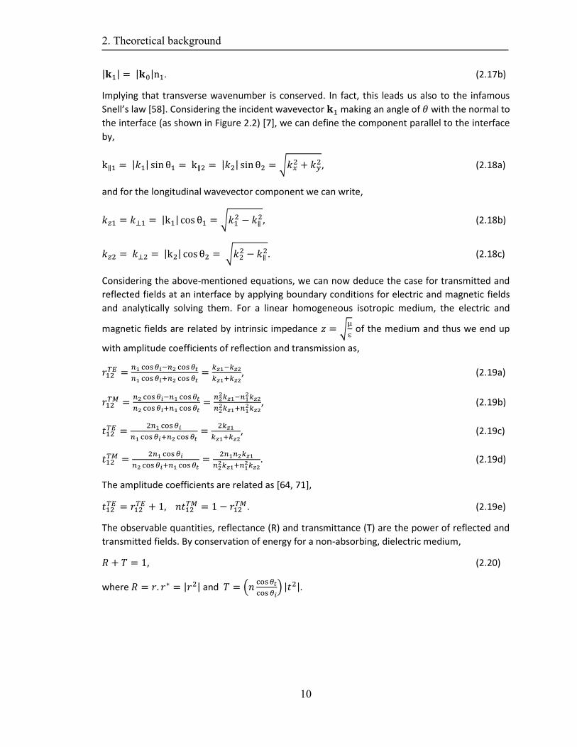
with amplitude coefficients of reflection and transmission as,
𝑟12𝑇𝐸 =
𝑛1 cos𝜃𝑖−𝑛2 cos𝜃𝑡
𝑛1 cos𝜃𝑖+𝑛2 cos𝜃𝑡=
𝑘𝑧1−𝑘𝑧2
𝑘𝑧1+𝑘𝑧2, (2.19a)
𝑟12𝑇𝑀 =
𝑛2 cos𝜃𝑖−𝑛1 cos𝜃𝑡
𝑛2 cos𝜃𝑖+𝑛1 cos𝜃𝑡=
𝑛22𝑘𝑧1−𝑛1
2𝑘𝑧2
𝑛22𝑘𝑧1+𝑛1
2𝑘𝑧2, (2.19b)
𝑡12𝑇𝐸 =
2𝑛1 cos𝜃𝑖
𝑛1 cos𝜃𝑖+𝑛2 cos𝜃𝑡=
2𝑘𝑧1
𝑘𝑧1+𝑘𝑧2, (2.19c)
𝑡12𝑇𝑀 =
2𝑛1 cos𝜃𝑖
𝑛2 cos𝜃𝑖+𝑛1 cos𝜃𝑡=
2𝑛1𝑛2𝑘𝑧1
𝑛22𝑘𝑧1+𝑛1
2𝑘𝑧2. (2.19d)
The amplitude coefficients are related as [64, 71],
𝑡12𝑇𝐸 = 𝑟12
𝑇𝐸 + 1, 𝑛𝑡12𝑇𝑀 = 1 − 𝑟12
𝑇𝑀. (2.19e)
The observable quantities, reflectance (R) and transmittance (T) are the power of reflected and
transmitted fields. By conservation of energy for a non-absorbing, dielectric medium,
𝑅 + 𝑇 = 1, (2.20)
where 𝑅 = 𝑟. 𝑟∗ = |𝑟2| and 𝑇 = (𝑛cos𝜃𝑡
cos𝜃𝑖) |𝑡2|.
2. Theoretical background
11
Figure 2.3 The propagation of TM (a) & TE (b) light fields at an interface. The Maxwell curl and
divergence equations leads us to the boundary condition for the tangential electric field and
normal displacement field components respectively being continuous. Implying that the
transverse wavenumber is conserved, leads us to the infamous Snell’s law.
Permittivity, permeability, and refractive index of a medium
From Maxwell’s equations, we can relate the electric displacement and field by the so-called
constitutive relations. Similar case can be assumed for the magnetic flux density and field. The
constitutive relations describe the medium’s interaction with the incoming electromagnetic fields
[58, 72]. These are shown as,
𝐃 = ε0𝐄 + 𝐏, (2.21a)
B= μ0(𝐇 + 𝐌). (2.22b)

2. Theoretical background
12
In Equations 2.16a and b, we introduce the mean dipole moment per unit volume expressed as
polarization and magnetization of a medium respectively (𝐏 and 𝐌). As in the previously described
case for boundary conditions (linear, homogenous, and isotropic), we can define polarization and
magnetization as,
𝐏 = ε0χe𝐄, also (1 + χe ) = εr , 𝐌 = μ0χm𝐇 , also (1 + χm ) = μr, (2.23)
where 𝜒𝑒 and 𝜒𝑚are the electric and magnetic susceptibility of the medium. 휀𝑟 and 𝜇𝑟 are the
relative permittivity and permeability of a medium (normalized with respect to free space values).
Essentially these equations serve as the starting point for understanding all sorts of light-matter
interaction. The Drude model for metals and Lorentz model for dielectrics and metals describes
the dependence of complex permittivity on angular frequency and material properties [64]. In
some instances, permittivity (휀) and permeability (𝜇) of a medium can take the form of a tensor
(anisotropic medium) or susceptibility could have higher order terms to define a nonlinear
medium response. Typically, naturally occurring materials have permittivity (휀) and permeability
(𝜇) that are dependent and change with angular frequency (𝜔). Usually, close to visible
frequencies the naturally occurring materials are non-magnetic meaning permeability close to
unity. The real part of permittivity is positive/negative, distinguishing between two naturally
occurring solids dielectrics/metals, respectively. These details will be important in later part of
this thesis regarding computation model for carbon flakes (built by our collaborator, Professor Dr.
Antonino Calà Lesina) and for considering chiroptical phenomenon.
Refractive index, which was used extensively in deriving boundary conditions, can also be related
to permittivity and permeability of a medium. Since permittivity is also a complex number and
assuming permeability being unity, a generalized form of refractive index can be expressed as a
complex number [64, 73],
�� = √𝜇𝑟휀𝑟 = 𝑛 + 𝑖𝜅, (2.24)
휀�� = 휀𝑟′ + 𝑖휀𝑟
′′, where 휀𝑟′ = 𝑛2 + 𝜅2 and 휀𝑟
′′ = 2𝑛𝜅, (2.25)
where 𝑛 / 𝜅 define the real/imaginary part of the refractive index, respectively. κ is also known as
extinction coefficient, which is related to the attenuation constant (α) by the relation, α =4𝜋𝜅
𝜆0,
where 𝜆0 is the wavelength of incident light onto the medium. 휀𝑟′ , 휀𝑟
′′ are the real and imaginary
part of complex permittivity, respectively. We also modify Equation 2.15 to accommodate
absorption in medium which now reads as,
R + T + A = 1, (2.26)
where A depicts the power of incident light beam absorbed by the interacting medium. We
discuss now two special conditions when refractive index of incident medium is lower than
transmission medium (𝑛2 > 𝑛1) , namely case for normal incidence and that of Brewster Effect
[74]. These two special conditions would later help us in defining the computational model used
for extracting refractive index.
2. Theoretical background
13
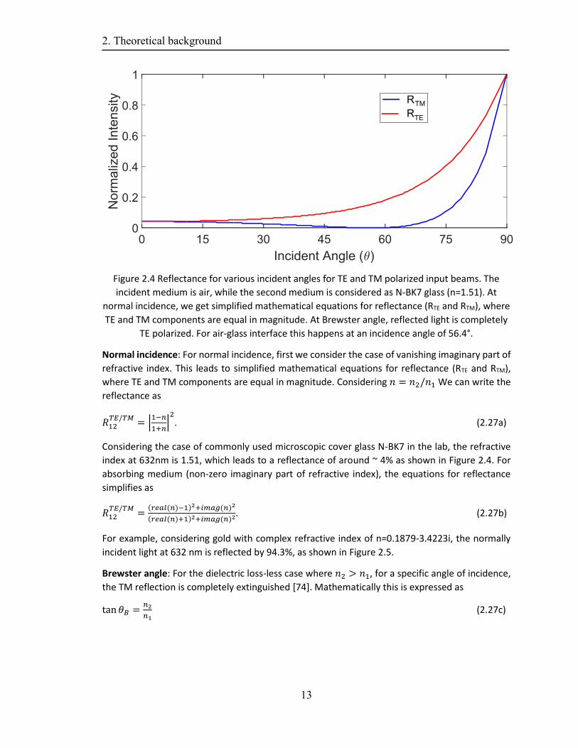
Figure 2.4 Reflectance for various incident angles for TE and TM polarized input beams. The
incident medium is air, while the second medium is considered as N-BK7 glass (n=1.51). At
normal incidence, we get simplified mathematical equations for reflectance (RTE and RTM), where
TE and TM components are equal in magnitude. At Brewster angle, reflected light is completely
TE polarized. For air-glass interface this happens at an incidence angle of 56.4°.
Normal incidence: For normal incidence, first we consider the case of vanishing imaginary part of
refractive index. This leads to simplified mathematical equations for reflectance (RTE and RTM),
where TE and TM components are equal in magnitude. Considering 𝑛 = 𝑛2/𝑛1 We can write the
reflectance as
𝑅12𝑇𝐸/𝑇𝑀
= |1−𝑛
1+𝑛|2. (2.27a)
Considering the case of commonly used microscopic cover glass N-BK7 in the lab, the refractive
index at 632nm is 1.51, which leads to a reflectance of around ~ 4% as shown in Figure 2.4. For
absorbing medium (non-zero imaginary part of refractive index), the equations for reflectance
simplifies as
𝑅12𝑇𝐸/𝑇𝑀
=(𝑟𝑒𝑎𝑙(𝑛)−1)2+𝑖𝑚𝑎𝑔(𝑛)2
(𝑟𝑒𝑎𝑙(𝑛)+1)2+𝑖𝑚𝑎𝑔(𝑛)2. (2.27b)
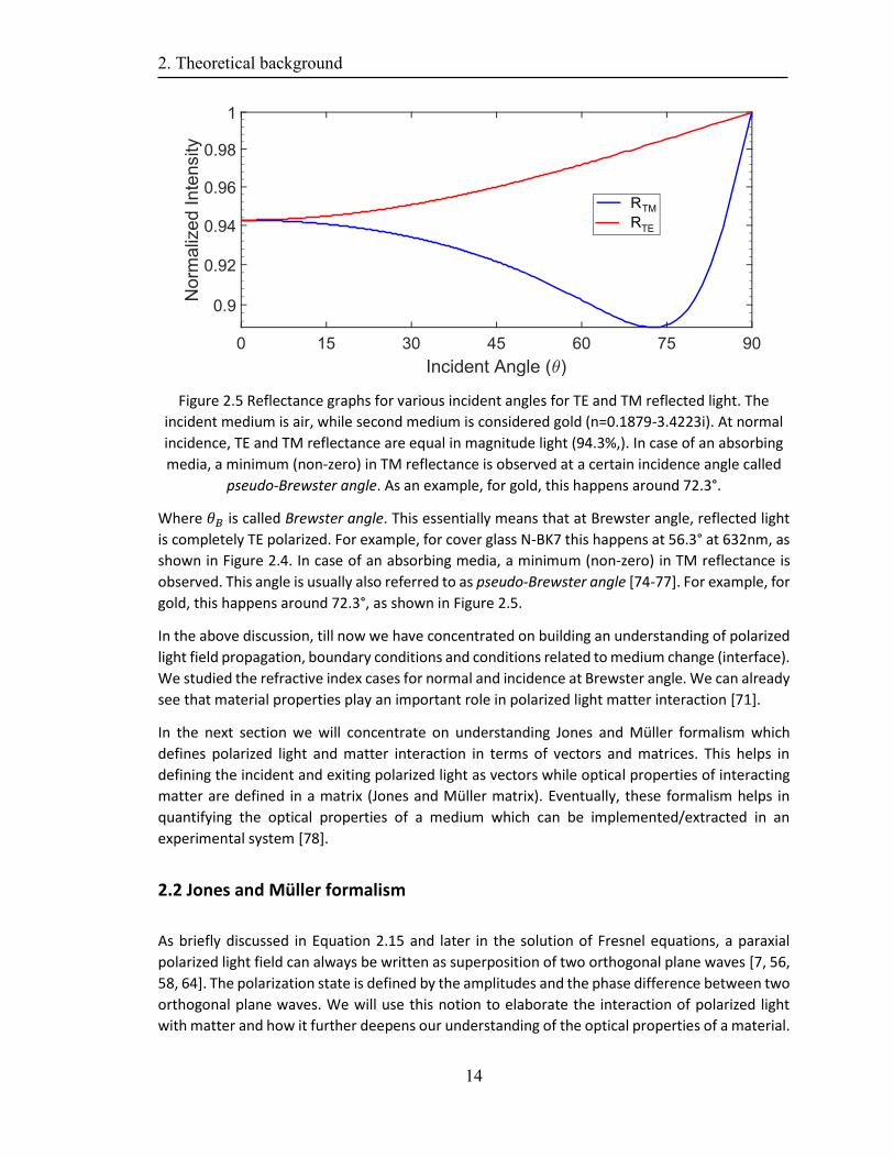
For example, considering gold with complex refractive index of n=0.1879-3.4223i, the normally
incident light at 632 nm is reflected by 94.3%, as shown in Figure 2.5.
Brewster angle: For the dielectric loss-less case where 𝑛2 > 𝑛1, for a specific angle of incidence,
the TM reflection is completely extinguished [74]. Mathematically this is expressed as
tan 𝜃𝐵 =𝑛2
𝑛1 (2.27c)
2. Theoretical background
14
Figure 2.5 Reflectance graphs for various incident angles for TE and TM reflected light. The
incident medium is air, while second medium is considered gold (n=0.1879-3.4223i). At normal
incidence, TE and TM reflectance are equal in magnitude light (94.3%,). In case of an absorbing
media, a minimum (non-zero) in TM reflectance is observed at a certain incidence angle called
pseudo-Brewster angle. As an example, for gold, this happens around 72.3°.
Where 𝜃𝐵 is called Brewster angle. This essentially means that at Brewster angle, reflected light
is completely TE polarized. For example, for cover glass N-BK7 this happens at 56.3° at 632nm, as
shown in Figure 2.4. In case of an absorbing media, a minimum (non-zero) in TM reflectance is
observed. This angle is usually also referred to as pseudo-Brewster angle [74-77]. For example, for
gold, this happens around 72.3°, as shown in Figure 2.5.
In the above discussion, till now we have concentrated on building an understanding of polarized
light field propagation, boundary conditions and conditions related to medium change (interface).
We studied the refractive index cases for normal and incidence at Brewster angle. We can already
see that material properties play an important role in polarized light matter interaction [71].
In the next section we will concentrate on understanding Jones and Müller formalism which
defines polarized light and matter interaction in terms of vectors and matrices. This helps in
defining the incident and exiting polarized light as vectors while optical properties of interacting
matter are defined in a matrix (Jones and Müller matrix). Eventually, these formalism helps in
quantifying the optical properties of a medium which can be implemented/extracted in an
experimental system [78].
2.2 Jones and Müller formalism
As briefly discussed in Equation 2.15 and later in the solution of Fresnel equations, a paraxial
polarized light field can always be written as superposition of two orthogonal plane waves [7, 56,
58, 64]. The polarization state is defined by the amplitudes and the phase difference between two
orthogonal plane waves. We will use this notion to elaborate the interaction of polarized light
with matter and how it further deepens our understanding of the optical properties of a material.
2. Theoretical background
15
Jones formalism
In 1941, the American physicist R. C. Jones, introduced a formalism based on Equation 2.16 to
define polarized light and its interaction with matter in a simple equation, now known as Jones
formalism [79]. We can write the Jones matrix and input and output light beam vectors together
mathematically as
(𝐄x
out
𝐄yout) = J (
𝐄xin
𝐄yin), (2.28)
where, the fields are related to respective incident and outgoing intensities by the relation,
𝐼𝑖𝑛/𝑜𝑢𝑡 = 𝐄in/out∗ 𝐄in/out and 𝐸∗define the complex conjugate of the respective field vector [58,
79, 80]. Here, the Jones matrix 𝐽 = (𝐽11 𝐽12
𝐽21 𝐽22) is a 2x2 matrix, which defines the optical
interaction of a medium with incident light beam. The terms of the Jones matrix are usually of
complex nature (amplitude and phase terms) and hence a total of 8 independent variables are
required to completely define the interaction of light with a medium [31]. We can also
conveniently define the interaction of light with multiple optical elements by cascaded
multiplication of respective Jones matrices (𝐽1 interacts first with the incident light beam). The
incident and outgoing light waves are then related as,
(𝐸𝑥
𝑜𝑢𝑡
𝐸𝑦𝑜𝑢𝑡) = (𝐽𝑛𝐽𝑛−1 …𝐽1) (
𝐄𝑥𝑖𝑛
𝐄𝑦𝑖𝑛) = 𝐽𝑡𝑜𝑡 (
𝐄𝑥𝑖𝑛
𝐄𝑦𝑖𝑛). (2.29)
As discussed above, each element of the Jones matrix is of complex nature (assuming the form
𝐴𝑒𝑖𝜑), where 𝐴 defines the amplitude and 𝜑 defines the phase associated with the respective
field component.
Amplitude ratios of Jones matrix
As it is evident from linear matrix calculations, real numbers in Jones matrix would correspond to
a changing ratio of orthogonal components of the incoming light wave. This can be thought of as
selective polarization absorber (e.g., polarizer) with arbitrary axis position (θ) leading to light
polarized at a certain azimuthal angle (θ) without introducing any phase difference.
Mathematically this matrix can then be written as,
𝐽𝑝𝑜𝑙 = ( cos2 𝜃 cos 𝜃 sin 𝜃cos 𝜃 sin𝜃 sin2 𝜃
) (2.30)
Phase ratios of Jones matrix
By adding certain phase to one field component of the incoming light, we can induce ellipticity
(𝜑) in the outgoing light wave [81, 82]. Optical materials (crystals) which can induce such an effect
have different refractive indices along orthogonal field components of the incoming light beam.
The generalized Jones matrix for a wave retarder is hence shown as,
𝐽𝑟𝑒𝑡𝑎𝑟𝑑𝑒𝑟 = (cos2 𝜃 + 𝑒𝑖𝛿sin2 𝜃 (1 − 𝑒𝑖𝛿)𝑒−𝑖𝜌cos𝜃 sin𝜃
(1 − 𝑒𝑖𝛿)𝑒𝑖𝜌cos 𝜃 sin 𝜃 𝑒𝑖𝛿cos2 𝜃 + sin2 𝜃), (2.31)
2. Theoretical background
16
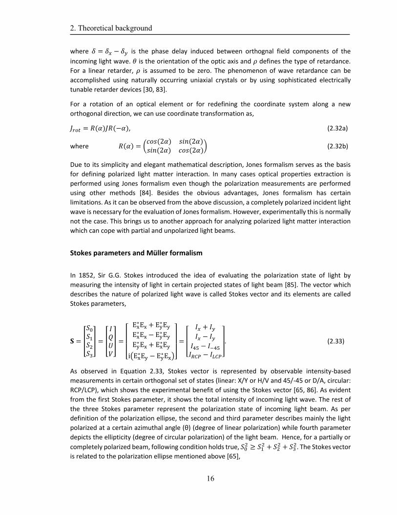
where 𝛿 = 𝛿𝑥 − 𝛿𝑦 is the phase delay induced between orthognal field components of the
incoming light wave. 𝜃 is the orientation of the optic axis and 𝜌 defines the type of retardance.
For a linear retarder, 𝜌 is assumed to be zero. The phenomenon of wave retardance can be
accomplished using naturally occurring uniaxial crystals or by using sophisticated electrically
tunable retarder devices [30, 83].
For a rotation of an optical element or for redefining the coordinate system along a new
orthogonal direction, we can use coordinate transformation as,
𝐽𝑟𝑜𝑡 = 𝑅(𝛼)𝐽𝑅(−𝛼), (2.32a)
where 𝑅(𝛼) = (𝑐𝑜𝑠(2𝛼) 𝑠𝑖𝑛(2𝛼)𝑠𝑖𝑛(2𝛼) 𝑐𝑜𝑠(2𝛼)
) (2.32b)
Due to its simplicity and elegant mathematical description, Jones formalism serves as the basis
for defining polarized light matter interaction. In many cases optical properties extraction is
performed using Jones formalism even though the polarization measurements are performed
using other methods [84]. Besides the obvious advantages, Jones formalism has certain
limitations. As it can be observed from the above discussion, a completely polarized incident light
wave is necessary for the evaluation of Jones formalism. However, experimentally this is normally
not the case. This brings us to another approach for analyzing polarized light matter interaction
which can cope with partial and unpolarized light beams.
Stokes parameters and Müller formalism
In 1852, Sir G.G. Stokes introduced the idea of evaluating the polarization state of light by
measuring the intensity of light in certain projected states of light beam [85]. The vector which
describes the nature of polarized light wave is called Stokes vector and its elements are called
Stokes parameters,
𝐒 = [
𝑆0
𝑆1
𝑆2
𝑆3
] = [
𝐼𝑄𝑈𝑉
] =
[
Ex∗Ex + Ey
∗Ey
Ex∗Ex − Ey
∗Ey
Ey∗Ex + Ex
∗Ey
i(Ex∗Ey − Ey
∗Ex)]
=
[
𝐼𝑥 + 𝐼𝑦𝐼𝑥 − 𝐼𝑦
𝐼45 − 𝐼−45
𝐼𝑅𝐶𝑃 − 𝐼𝐿𝐶𝑃] . (2.33)
As observed in Equation 2.33, Stokes vector is represented by observable intensity-based
measurements in certain orthogonal set of states (linear: X/Y or H/V and 45/-45 or D/A, circular:
RCP/LCP), which shows the experimental benefit of using the Stokes vector [65, 86]. As evident
from the first Stokes parameter, it shows the total intensity of incoming light wave. The rest of
the three Stokes parameter represent the polarization state of incoming light beam. As per
definition of the polarization ellipse, the second and third parameter describes mainly the light
polarized at a certain azimuthal angle (θ) (degree of linear polarization) while fourth parameter
depicts the ellipticity (degree of circular polarization) of the light beam. Hence, for a partially or
completely polarized beam, following condition holds true, 𝑆02 ≥ 𝑆1
2 + 𝑆22 + 𝑆3
2. The Stokes vector
is related to the polarization ellipse mentioned above [65],
2. Theoretical background
17
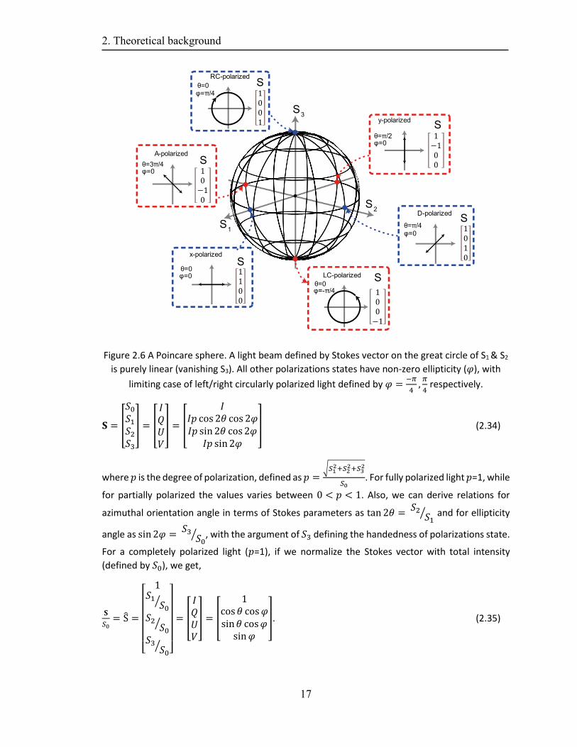
Figure 2.6 A Poincare sphere. A light beam defined by Stokes vector on the great circle of S1 & S2
is purely linear (vanishing S3). All other polarizations states have non-zero ellipticity (𝜑), with
limiting case of left/right circularly polarized light defined by 𝜑 =−𝜋
4,𝜋
4 respectively.
𝐒 = [
𝑆0
𝑆1
𝑆2
𝑆3
] = [
𝐼𝑄𝑈𝑉
] = [
𝐼𝐼𝑝 cos 2𝜃 cos 2𝜑𝐼𝑝 sin2𝜃 cos2𝜑
𝐼𝑝 sin2𝜑
] (2.34)
where 𝑝 is the degree of polarization, defined as 𝑝 =√𝑆1
2+𝑆22+𝑆3
2
𝑆0. For fully polarized light 𝑝=1, while
for partially polarized the values varies between 0 < 𝑝 < 1. Also, we can derive relations for
azimuthal orientation angle in terms of Stokes parameters as tan 2𝜃 = 𝑆2
𝑆1⁄ and for ellipticity
angle as sin2𝜑 = 𝑆3
𝑆0⁄ , with the argument of 𝑆3 defining the handedness of polarizations state.
For a completely polarized light (𝑝=1), if we normalize the Stokes vector with total intensity
(defined by 𝑆0), we get,
𝐒
𝑆0= S =
[
1𝑆1
𝑆0⁄
𝑆2𝑆0
⁄
𝑆3𝑆0
⁄ ]
= [
𝐼𝑄𝑈𝑉
] = [
1cos𝜃 cos𝜑sin𝜃 cos𝜑
sin𝜑
]. (2.35)
2. Theoretical background
18
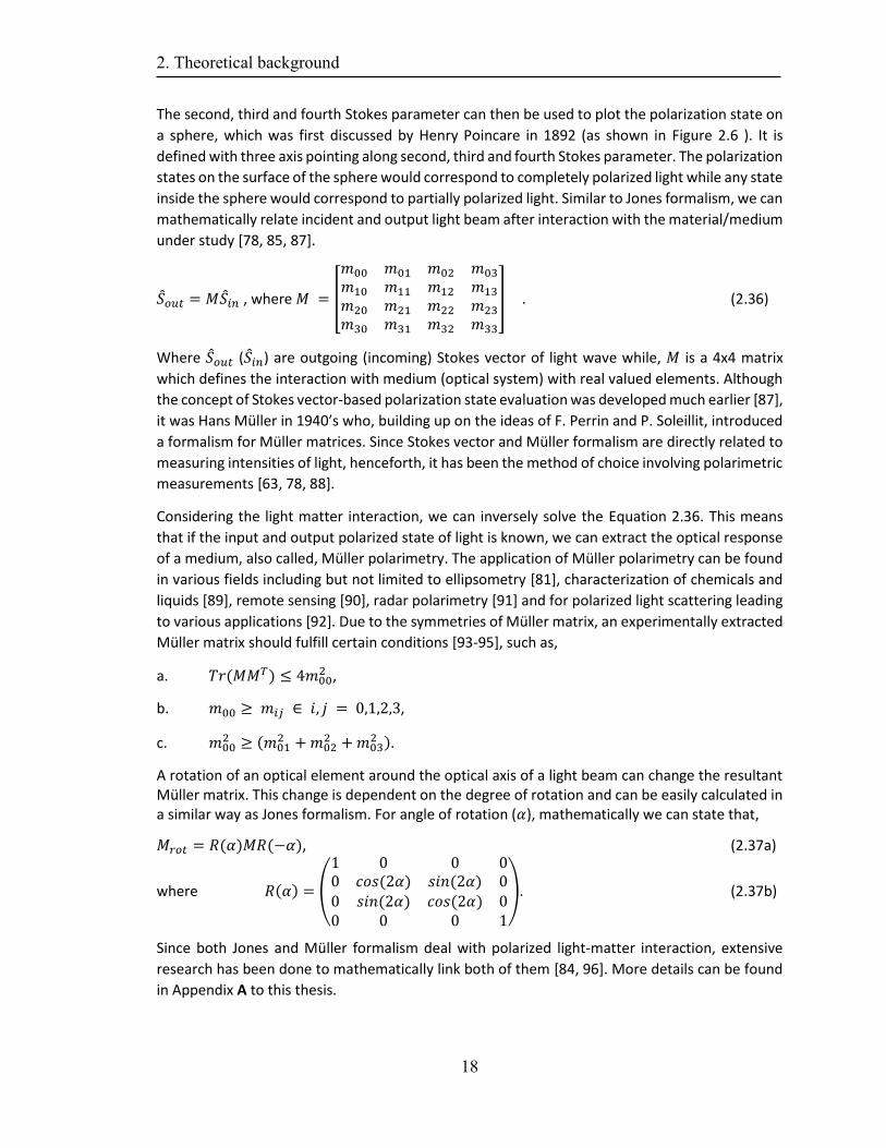
The second, third and fourth Stokes parameter can then be used to plot the polarization state on
a sphere, which was first discussed by Henry Poincare in 1892 (as shown in Figure 2.6 ). It is
defined with three axis pointing along second, third and fourth Stokes parameter. The polarization
states on the surface of the sphere would correspond to completely polarized light while any state
inside the sphere would correspond to partially polarized light. Similar to Jones formalism, we can
mathematically relate incident and output light beam after interaction with the material/medium
under study [78, 85, 87].
��𝑜𝑢𝑡 = 𝑀��𝑖𝑛 , where 𝑀 = [
𝑚00 𝑚01 𝑚02 𝑚03
𝑚10 𝑚11 𝑚12 𝑚13
𝑚20 𝑚21 𝑚22 𝑚23
𝑚30 𝑚31 𝑚32 𝑚33
] . (2.36)
Where ��𝑜𝑢𝑡 (��𝑖𝑛) are outgoing (incoming) Stokes vector of light wave while, 𝑀 is a 4x4 matrix
which defines the interaction with medium (optical system) with real valued elements. Although
the concept of Stokes vector-based polarization state evaluation was developed much earlier [87],
it was Hans Müller in 1940’s who, building up on the ideas of F. Perrin and P. Soleillit, introduced
a formalism for Müller matrices. Since Stokes vector and Müller formalism are directly related to
measuring intensities of light, henceforth, it has been the method of choice involving polarimetric
measurements [63, 78, 88].
Considering the light matter interaction, we can inversely solve the Equation 2.36. This means
that if the input and output polarized state of light is known, we can extract the optical response
of a medium, also called, Müller polarimetry. The application of Müller polarimetry can be found
in various fields including but not limited to ellipsometry [81], characterization of chemicals and
liquids [89], remote sensing [90], radar polarimetry [91] and for polarized light scattering leading
to various applications [92]. Due to the symmetries of Müller matrix, an experimentally extracted
Müller matrix should fulfill certain conditions [93-95], such as,
a. 𝑇𝑟(𝑀𝑀𝑇) ≤ 4𝑚002 ,
b. 𝑚00 ≥ 𝑚𝑖𝑗 ∈ 𝑖, 𝑗 = 0,1,2,3,
c. 𝑚002 ≥ (𝑚01
2 + 𝑚022 + 𝑚03
2 ).
A rotation of an optical element around the optical axis of a light beam can change the resultant Müller matrix. This change is dependent on the degree of rotation and can be easily calculated in a similar way as Jones formalism. For angle of rotation (𝛼), mathematically we can state that,
𝑀𝑟𝑜𝑡 = 𝑅(𝛼)𝑀𝑅(−𝛼), (2.37a)
where 𝑅(𝛼) = (
1 0 0 00 𝑐𝑜𝑠(2𝛼) 𝑠𝑖𝑛(2𝛼) 00 𝑠𝑖𝑛(2𝛼) 𝑐𝑜𝑠(2𝛼) 00 0 0 1
). (2.37b)
Since both Jones and Müller formalism deal with polarized light-matter interaction, extensive
research has been done to mathematically link both of them [84, 96]. More details can be found
in Appendix A to this thesis.
2. Theoretical background
19
2.3 Optical material properties
In this section, we will elaborate on the optical properties of an examined medium and relevant
mathematical techniques to extract these properties from an experimental Müller matrix. We will
discuss some common setups for determining the Müller matrix of an examined material. Later,
we will elaborate the concept of complex refractive index retrieval and discuss the computational
model for that process.
Optical properties from Müller matrix
Here, we will briefly discuss optical properties that can be extracted from a Müller matrix. These
can be broadly categorized as, depolarization, dichroism, and birefringence of a medium. We
consider the case of Müller matrix in transmission.
Depolarization of incident light
This describes the phenomenon in which polarized light is coupled into depolarized light. It can
intrinsically happen in case of scattering or for loss of coherence in a polarized light wave. The
Müller matrix for a depolarizer can be shown as [63],
𝑀𝑑𝑒𝑝𝑜𝑙 = [
1 0 0 00 𝑝𝑥,𝑦 0 0
0 0 𝑝𝐴,𝐷 0
0 0 0 𝑐𝑝
], (2.38)
where 𝑝, 𝑝45 and 𝑝45 are the depolarization along horizontal, diagonal, and circular polarization
states, respectively. Another way to describe depolarization is also as the variation in degree of
polarization of light as discussed earlier. In an optical experiment, depolarization can lead to
unrealizable experimental results and therefore, needs to be identified and removed accordingly
[63, 71, 93, 95, 97-99].
Dichroism of a medium
Dichroism is the phenomenon whereby an incident light beam travelling through a medium
encounter differential extinction. The outgoing intensity can be maximum along one field
component while minimum along the other orthogonal field component of exiting light beam.
This optical phenomenon can also be understood as the difference in imaginary part of refractive
index, i.e., extinction coefficient along two orthogonal directions for a medium Mathematically
this can be defined as,
𝐷 =𝐼𝑚𝑎𝑥 − 𝐼𝑚𝑖𝑛
𝐼𝑚𝑎𝑥 +𝐼𝑚𝑖𝑛, (2.39a)
𝐷 =(𝜅𝑎−𝜅𝑏)𝜆
2𝜋𝑙, (2.39b)
where 𝜅 is the extinction coefficient, 𝑙 is the length for which light propagates through the
medium and a, b represents the orthogonal polarization projection. Based on the mathematical
2. Theoretical background
20
definition of the Stokes vector, we can define three polarization projection sets, which are as
follows,
𝐿𝑖𝑛𝑒𝑎𝑟 𝐷𝑖𝑐ℎ𝑟𝑜𝑖𝑠𝑚 = 𝐿𝐷 =(𝜅𝑥−𝜅𝑦)𝜆
2𝜋𝑙 , (2.39c)
𝐿𝐷45 =(𝜅45−𝜅−45)𝜆
2𝜋𝑙 , (2.39d)
𝐶𝑟𝑖𝑐𝑢𝑙𝑎𝑟 𝐷𝑖𝑐ℎ𝑟𝑜𝑖𝑠𝑚 = 𝐶𝐷 =(𝜅𝑅𝐶𝑃−𝜅𝐿𝐶𝑃)𝜆
2𝜋𝑙 . (2.39e)
The information regarding dichroism of a material can be found in the first row and column of
respective Müller matrix of the medium. Linear polarizers are a good example of a material
possessing linear dichroism. The case of circular dichroism leads to chirality in a medium which
will be discussed in Chapter 4 of this thesis.
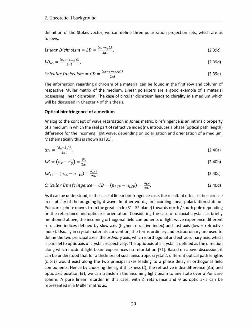
Optical birefringence of a medium
Analog to the concept of wave retardation in Jones matrix, birefringence is an intrinsic property
of a medium in which the real part of refractive index (n), introduces a phase (optical path length)
difference for the incoming light wave, depending on polarization and orientation of a medium.
Mathematically this is shown as [81],
∆n =(𝛿𝑎−𝛿𝑏)𝜆
2𝜋𝑙, (2.40a)
𝐿𝐵 = (𝑛𝑥 − 𝑛𝑦) =𝛿𝜆
2𝜋𝑙 , (2.40b)
𝐿𝐵45 = (𝑛45 − 𝑛−45) =𝛿45𝜆
2𝜋𝑙, (2.40c)
𝐶𝑟𝑖𝑐𝑢𝑙𝑎𝑟 𝐵𝑖𝑟𝑒𝑓𝑟𝑖𝑛𝑔𝑒𝑛𝑐𝑒 = 𝐶𝐵 = (𝑛𝑅𝐶𝑃 − 𝑛𝐿𝐶𝑃) =𝛿𝐶𝜆
2𝜋𝑙. (2.40d)
As it can be understood, in the case of linear birefringence case, the resultant effect is the increase
in ellipticity of the outgoing light wave. In other words, an incoming linear polarization state on
Poincare sphere moves from the great circle (S1 - S2 plane) towards north / south pole depending
on the retardance and optic axis orientation. Considering the case of uniaxial crystals as briefly
mentioned above, the incoming orthogonal field components of light wave experience different
refractive indices defined by slow axis (higher refractive index) and fast axis (lower refractive
index). Usually in crystal materials convention, the terms ordinary and extraordinary are used to
define the two principal axes: the ordinary axis, which is orthogonal and extraordinary axis, which
is parallel to optic axis of crystal, respectively. The optic axis of a crystal is defined as the direction
along which incident light beam experiences no retardation [71]. Based on above discussion, it
can be understood that for a thickness of such anisotropic crystal 𝑙, different optical path lengths
(𝑛 × 𝑙) would exist along the two principal axes leading to a phase delay in orthogonal field
components. Hence by choosing the right thickness (𝑙), the refractive index difference (∆n) and
optic axis position (𝜃), we can transform the incoming light beam to any state over a Poincare
sphere. A pure linear retarder in this case, with 𝛿 retardance and θ as optic axis can be
represented in a Müller matrix as,
2. Theoretical background
21
𝑀 =
(
1 0 0 00 𝑐𝑜𝑠2(2𝜃) + 𝑠𝑖𝑛2(2𝜃)𝑐𝑜𝑠(𝛿) 𝑠𝑖𝑛(2𝜃)𝑐𝑜𝑠(2𝜃)(1 − 𝑐𝑜𝑠(𝛿)) −𝑠𝑖𝑛(2𝜃)𝑠𝑖𝑛(𝛿)
0 𝑠𝑖𝑛(2𝜃)𝑐𝑜𝑠(2𝜃)(1 − 𝑐𝑜𝑠(𝛿)) 𝑠𝑖𝑛2(2𝜃) + 𝑐𝑜𝑠2(2𝜃)𝑐𝑜𝑠(𝛿) 𝑐𝑜𝑠(2𝜃)𝑠𝑖𝑛(𝛿)
0 𝑠𝑖𝑛(2𝜃)𝑠𝑖𝑛(𝛿) −𝑐𝑜𝑠(2𝜃)𝑠𝑖𝑛(𝛿) 𝑐𝑜𝑠(𝛿) )
. (2.41)
Müller matrices and optical systems
As discussed above, Müller matrix can describe a set of properties which can help define optical
response of a medium. It is also pertinent to differentiate between observable quantities and
intrinsic properties of a system. For instance, extinction is an observable quantity which
depending on the length of the medium and wavelength of incoming light wave, defines
dichroism. Similar is the case for the observable transmission/retardance, which are related to
attenuation/birefringence, of a medium, respectively. For an optical system possessing
abovementioned optical properties, it can be directly correlated to a certain element of
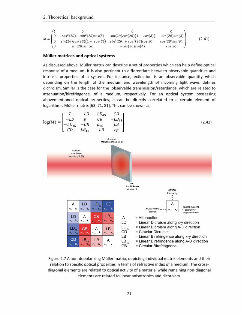
logarithmic Müller matrix [63, 71, 81]. This can be shown as,
log(𝑀) = [
𝑇 −𝐿𝐷 −𝐿𝐷45 𝐶𝐷−𝐿𝐷 𝑝 𝐶𝑅 −𝐿𝐵45
−𝐿𝐷45 −𝐶𝑅 𝑝45 𝐿𝐵𝐶𝐷 𝐿𝐵45 −𝐿𝐵 𝑐𝑝
]. (2.42)
Figure 2.7 A non-depolarizing Müller matrix, depicting individual matrix elements and their
relation to specific optical properties in terms of refractive index of a medium. The cross-
diagonal elements are related to optical activity of a material while remaining non-diagonal
elements are related to linear anisotropies and dichroism.
2. Theoretical background
22
It is important to highlight that Equation 2.42 represents element wise association of optical
properties. If we consider an isotropic, homogenous, non-depolarizing absorbing medium, we can
expect the diagonal terms to depict attenuation experienced by an incoming light beam, as shown
in Equation 2.42 and Figure 2.7.
As discussed in Equation 2.40(a-d), anisotropic medium possesses different refractive indices
along principal axis of medium. The relevant anisotropic information of a medium is present in off
diagonal elements shown as in Equation 2.42 and Figure 2.7. We can see that the differential
extinction and linear retardance effects are segregated in upper right and lower left corner of
Müller matrix, respectively. Because of the cross interaction of linear dichroism and birefringence
we can expect 𝑚12 & 𝑚21 to have residual values, although these elements also depict chiral
effects [97, 100]. For an ideal linear retarder and attenuator, we can expect 𝑚12 & 𝑚21 to be
equal in magnitude and have the same sign.
Isotropic chiral media
For definition of chiral media as discussed above, we can expect circular dichroism and retardance
from such a medium. As shown in Equation 2.42 and Figure 2.7, the cross-diagonal terms depict
the chiral properties of the medium. It should be noted that for reciprocal system 𝑚03& 𝑚30 have
same sign and magnitude, while for non-reciprocal system we can expect opposite sign of these
matrix elements. A detailed description of reciprocal/ non-reciprocal systems and their
comparison to chiral response of a medium can be found in Appendix A to this thesis. Typically,
circular retardance are small in magnitude (10-3 and lower) and hence experimentally difficult to
detect. A common experimental technique in this case is to measure circular retardance along the
optic axis of anisotropic medium (thus avoiding optical effects from linear retardance).
Polarimetric systems and Müller matrix decomposition
To experimentally record information regarding polarized light matter interaction, different
schemes are employed, which eventually are computationally evaluated to extract Müller matrix.
Some of the existing commercially available techniques/polarimetric setups are briefly mentioned
below.
Müller matrix-based polarimetry
Based on the Müller matrix approach, different polarization measurement systems are designed.
A Müller matrix is computationally extracted from the input and output Stokes vector as discussed
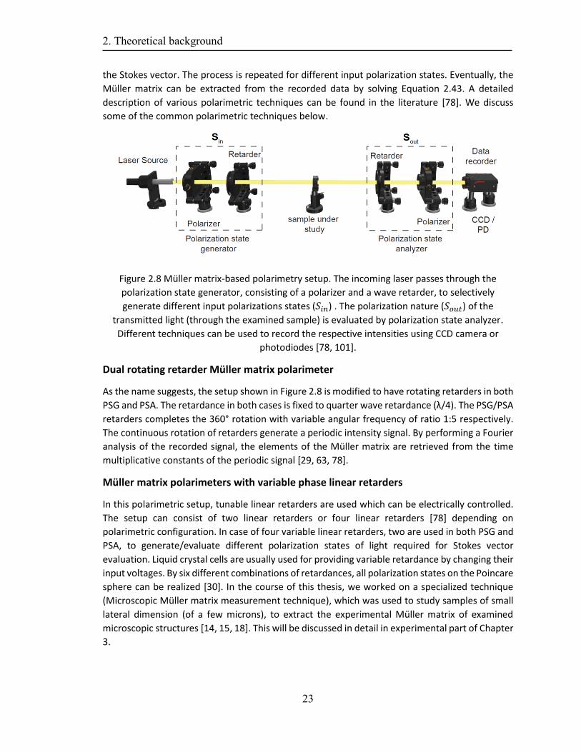
above. A generic structure of a Müller matrix based polarimeter is shown in Figure 2.8 [78]. The
incoming laser passes through the polarization state generator (PSG), consisting of a polarizer and
a wave retarder, to selectively generate different input polarizations states. After passing through
the sample, the light beam is projected into 6 polarizations states (H, V, A, D, RC & LC) necessary
for Stokes vector using polarizing state analyzer (PSA). Different techniques can be used to record
the respective intensities using CCD camera or photodiodes. The main difference in different
approaches is based on the three main components namely PSG, PSA and detectors. One of the
commonly used method involves using a quarter-wave retarder with a polarizer in PSA. By
rotating the QWP to certain angular positions and recording respective intensity, we can extract
2. Theoretical background
23
the Stokes vector. The process is repeated for different input polarization states. Eventually, the
Müller matrix can be extracted from the recorded data by solving Equation 2.43. A detailed
description of various polarimetric techniques can be found in the literature [78]. We discuss
some of the common polarimetric techniques below.
Figure 2.8 Müller matrix-based polarimetry setup. The incoming laser passes through the
polarization state generator, consisting of a polarizer and a wave retarder, to selectively
generate different input polarizations states (𝑆𝑖𝑛) . The polarization nature (𝑆𝑜𝑢𝑡) of the
transmitted light (through the examined sample) is evaluated by polarization state analyzer.
Different techniques can be used to record the respective intensities using CCD camera or
photodiodes [78, 101].
Dual rotating retarder Müller matrix polarimeter
As the name suggests, the setup shown in Figure 2.8 is modified to have rotating retarders in both
PSG and PSA. The retardance in both cases is fixed to quarter wave retardance (λ/4). The PSG/PSA
retarders completes the 360° rotation with variable angular frequency of ratio 1:5 respectively.
The continuous rotation of retarders generate a periodic intensity signal. By performing a Fourier
analysis of the recorded signal, the elements of the Müller matrix are retrieved from the time
multiplicative constants of the periodic signal [29, 63, 78].
Müller matrix polarimeters with variable phase linear retarders
In this polarimetric setup, tunable linear retarders are used which can be electrically controlled.
The setup can consist of two linear retarders or four linear retarders [78] depending on
polarimetric configuration. In case of four variable linear retarders, two are used in both PSG and
PSA, to generate/evaluate different polarization states of light required for Stokes vector
evaluation. Liquid crystal cells are usually used for providing variable retardance by changing their
input voltages. By six different combinations of retardances, all polarization states on the Poincare
sphere can be realized [30]. In the course of this thesis, we worked on a specialized technique
(Microscopic Müller matrix measurement technique), which was used to study samples of small
lateral dimension (of a few microns), to extract the experimental Müller matrix of examined
microscopic structures [14, 15, 18]. This will be discussed in detail in experimental part of Chapter
3.
2. Theoretical background
24
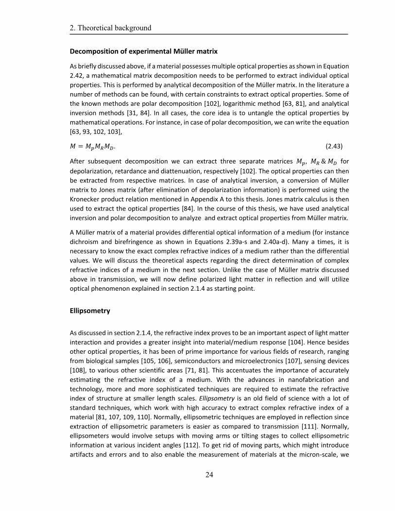
Decomposition of experimental Müller matrix
As briefly discussed above, if a material possesses multiple optical properties as shown in Equation
2.42, a mathematical matrix decomposition needs to be performed to extract individual optical
properties. This is performed by analytical decomposition of the Müller matrix. In the literature a
number of methods can be found, with certain constraints to extract optical properties. Some of
the known methods are polar decomposition [102], logarithmic method [63, 81], and analytical
inversion methods [31, 84]. In all cases, the core idea is to untangle the optical properties by
mathematical operations. For instance, in case of polar decomposition, we can write the equation
[63, 93, 102, 103],
𝑀 = 𝑀𝑝𝑀𝑅𝑀𝐷. (2.43)
After subsequent decomposition we can extract three separate matrices 𝑀𝑝, 𝑀𝑅 & 𝑀𝐷 for
depolarization, retardance and diattenuation, respectively [102]. The optical properties can then
be extracted from respective matrices. In case of analytical inversion, a conversion of Müller
matrix to Jones matrix (after elimination of depolarization information) is performed using the
Kronecker product relation mentioned in Appendix A to this thesis. Jones matrix calculus is then
used to extract the optical properties [84]. In the course of this thesis, we have used analytical
inversion and polar decomposition to analyze and extract optical properties from Müller matrix.
A Müller matrix of a material provides differential optical information of a medium (for instance
dichroism and birefringence as shown in Equations 2.39a-s and 2.40a-d). Many a times, it is
necessary to know the exact complex refractive indices of a medium rather than the differential
values. We will discuss the theoretical aspects regarding the direct determination of complex
refractive indices of a medium in the next section. Unlike the case of Müller matrix discussed
above in transmission, we will now define polarized light matter in reflection and will utilize
optical phenomenon explained in section 2.1.4 as starting point.
Ellipsometry
As discussed in section 2.1.4, the refractive index proves to be an important aspect of light matter
interaction and provides a greater insight into material/medium response [104]. Hence besides
other optical properties, it has been of prime importance for various fields of research, ranging
from biological samples [105, 106], semiconductors and microelectronics [107], sensing devices
[108], to various other scientific areas [71, 81]. This accentuates the importance of accurately
estimating the refractive index of a medium. With the advances in nanofabrication and
technology, more and more sophisticated techniques are required to estimate the refractive
index of structure at smaller length scales. Ellipsometry is an old field of science with a lot of
standard techniques, which work with high accuracy to extract complex refractive index of a
material [81, 107, 109, 110]. Normally, ellipsometric techniques are employed in reflection since
extraction of ellipsometric parameters is easier as compared to transmission [111]. Normally,
ellipsometers would involve setups with moving arms or tilting stages to collect ellipsometric
information at various incident angles [112]. To get rid of moving parts, which might introduce
artifacts and errors and to also enable the measurement of materials at the micron-scale, we
2. Theoretical background
25
extend the capabilities of conventional ellipsometry with back focal plane imaging and structured
illumination. As discussed in Equation 2.12, focused light provides for a large angular spectrum
(multiple angles of incidence) [62] and, hence, might allow for the retrieval of ellipsometric data
in a single measurement [113]. A simple step towards this idea was reported recently using
structured light to extract the real part of the refractive index for dielectric media (negligible
absorption) [114]. The main concept is based on vanishing reflectance for TM polarized light at
certain incidence angle (Brewster effect) [74] to extract refractive index exploiting greater angular
spectrum offered by high NA microscope objective [115, 116]. Here, we will discuss computational
methods to extend the technique to the case of complex refractive index retrieval. We will use
the far-field angular spectrum representation for studying the interaction of tightly focused light
with a medium in reflection, and discuss how it can be utilized to extract complex refractive index
[117]. Later, we will define the computational fitting model, which can be used to extract the
required ellipsometric parameters. Later, in the next chapter we will discuss the experimental
setup and results for certain materials tested.
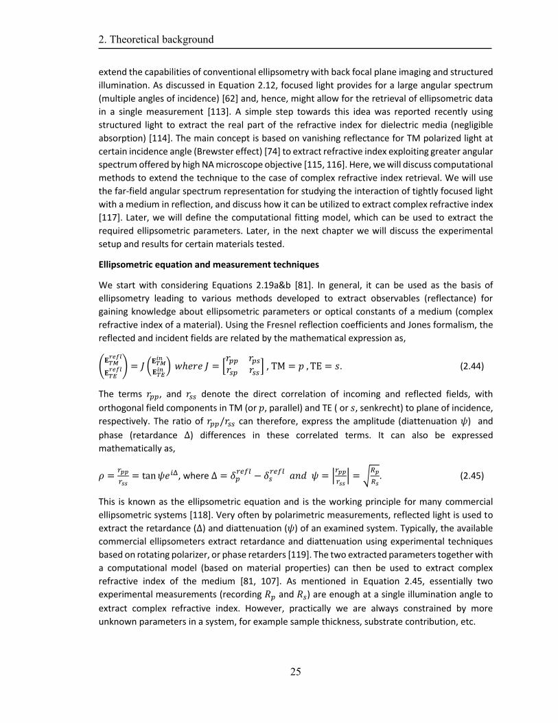
Ellipsometric equation and measurement techniques
We start with considering Equations 2.19a&b [81]. In general, it can be used as the basis of
ellipsometry leading to various methods developed to extract observables (reflectance) for
gaining knowledge about ellipsometric parameters or optical constants of a medium (complex
refractive index of a material). Using the Fresnel reflection coefficients and Jones formalism, the
reflected and incident fields are related by the mathematical expression as,
(𝐄𝑇𝑀
𝑟𝑒𝑓𝑙
𝐄𝑇𝐸𝑟𝑒𝑓𝑙) = 𝐽 (
𝐄𝑇𝑀𝑖𝑛
𝐄𝑇𝐸𝑖𝑛 ) 𝑤ℎ𝑒𝑟𝑒 𝐽 = [
𝑟𝑝𝑝 𝑟𝑝𝑠
𝑟𝑠𝑝 𝑟𝑠𝑠] , TM = 𝑝 , TE = 𝑠. (2.44)
The terms 𝑟𝑝𝑝, and 𝑟𝑠𝑠 denote the direct correlation of incoming and reflected fields, with
orthogonal field components in TM (or 𝑝, parallel) and TE ( or 𝑠, senkrecht) to plane of incidence,
respectively. The ratio of 𝑟𝑝𝑝/𝑟𝑠𝑠 can therefore, express the amplitude (diattenuation 𝜓) and
phase (retardance Δ) differences in these correlated terms. It can also be expressed
mathematically as,
𝜌 =𝑟𝑝𝑝
𝑟𝑠𝑠= tan𝜓𝑒𝑖Δ, where Δ = 𝛿𝑝
𝑟𝑒𝑓𝑙− 𝛿𝑠
𝑟𝑒𝑓𝑙 𝑎𝑛𝑑 𝜓 = |
𝑟𝑝𝑝
𝑟𝑠𝑠| = √
𝑅𝑝
𝑅𝑠. (2.45)
This is known as the ellipsometric equation and is the working principle for many commercial
ellipsometric systems [118]. Very often by polarimetric measurements, reflected light is used to
extract the retardance (Δ) and diattenuation (𝜓) of an examined system. Typically, the available
commercial ellipsometers extract retardance and diattenuation using experimental techniques
based on rotating polarizer, or phase retarders [119]. The two extracted parameters together with
a computational model (based on material properties) can then be used to extract complex
refractive index of the medium [81, 107]. As mentioned in Equation 2.45, essentially two
experimental measurements (recording 𝑅𝑝 and 𝑅𝑠) are enough at a single illumination angle to
extract complex refractive index. However, practically we are always constrained by more
unknown parameters in a system, for example sample thickness, substrate contribution, etc.
2. Theoretical background
26
This is then catered by performing a sweep over a certain variable input and later using a curve
fitting model to extract refractive index [81, 107, 109, 110, 120]. Two common variable input are
wavelength and multiple angles of illumination (MAI), also known as spectroscopic ellipsometry
[118] or MAI ellipsometry [116, 120]. Methods that record experimental data over a wavelength
range and then perform material model fitting comes under spectroscopic ellipsometry. These
systems however have spatial resolution in tens of microns making them convenient for thin films
characterization.
Techniques that record data over a range of angle of incidence to extract complex refractive index
are known as MAI ellipsometry. A common example is of exploiting Brewster effect to gain access
to refractive index of a medium [75-77, 114, 117, 121, 122]. Usually, it involves a goniometer stage
to change incident angle of light beam with respect to sample. Usually a range of incidence angle
from 35-70° is used [96]. A major disadvantage in this case is that the technique involves moving
mechanical parts and becomes more complex for multilayer systems, leading to inaccuracies in
refractive index estimation. Another example of MAI ellipsometry is based on the principal angle
[96]. The incident angle 𝜃𝑝 for which TE and TM components of the reflected field has a phase
difference of π/2 is called principal angle. If a diagonal (45°) polarized light is used as incident
beam, then in reflection at principal angle we will have right circularly polarized light.
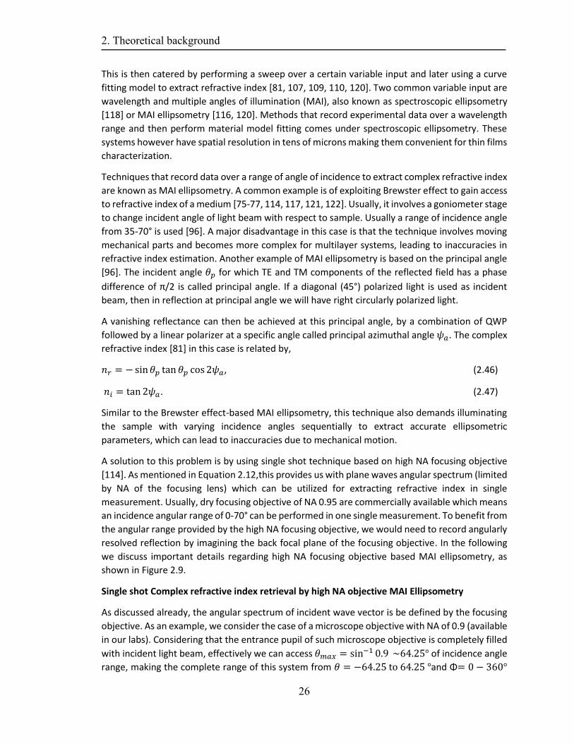
A vanishing reflectance can then be achieved at this principal angle, by a combination of QWP
followed by a linear polarizer at a specific angle called principal azimuthal angle 𝜓𝑎. The complex
refractive index [81] in this case is related by,
𝑛𝑟 = −sin𝜃𝑝 tan 𝜃𝑝 cos2𝜓𝑎, (2.46)
𝑛𝑖 = tan2𝜓𝑎. (2.47)
Similar to the Brewster effect-based MAI ellipsometry, this technique also demands illuminating
the sample with varying incidence angles sequentially to extract accurate ellipsometric
parameters, which can lead to inaccuracies due to mechanical motion.
A solution to this problem is by using single shot technique based on high NA focusing objective
[114]. As mentioned in Equation 2.12,this provides us with plane waves angular spectrum (limited
by NA of the focusing lens) which can be utilized for extracting refractive index in single
measurement. Usually, dry focusing objective of NA 0.95 are commercially available which means
an incidence angular range of 0-70° can be performed in one single measurement. To benefit from
the angular range provided by the high NA focusing objective, we would need to record angularly
resolved reflection by imagining the back focal plane of the focusing objective. In the following
we discuss important details regarding high NA focusing objective based MAI ellipsometry, as
shown in Figure 2.9.
Single shot Complex refractive index retrieval by high NA objective MAI Ellipsometry
As discussed already, the angular spectrum of incident wave vector is be defined by the focusing
objective. As an example, we consider the case of a microscope objective with NA of 0.9 (available
in our labs). Considering that the entrance pupil of such microscope objective is completely filled
with incident light beam, effectively we can access 𝜃𝑚𝑎𝑥 = sin−1 0.9 ~64.25° of incidence angle
range, making the complete range of this system from 𝜃 = −64.25 to 64.25 °and Φ= 0 − 360°
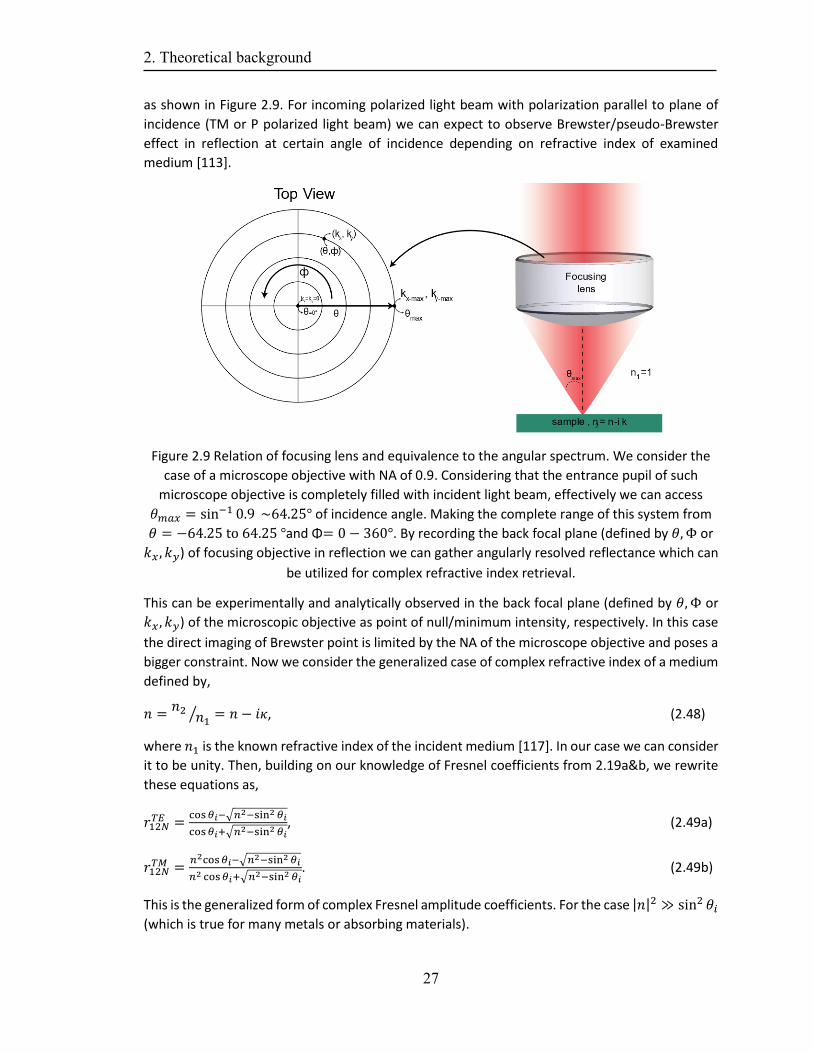
2. Theoretical background
27
as shown in Figure 2.9. For incoming polarized light beam with polarization parallel to plane of
incidence (TM or P polarized light beam) we can expect to observe Brewster/pseudo-Brewster
effect in reflection at certain angle of incidence depending on refractive index of examined
medium [113].
Figure 2.9 Relation of focusing lens and equivalence to the angular spectrum. We consider the
case of a microscope objective with NA of 0.9. Considering that the entrance pupil of such
microscope objective is completely filled with incident light beam, effectively we can access
𝜃𝑚𝑎𝑥 = sin−1 0.9 ~64.25° of incidence angle. Making the complete range of this system from
𝜃 = −64.25 to 64.25 °and Φ= 0 − 360°. By recording the back focal plane (defined by 𝜃,Φ or
𝑘𝑥 , 𝑘𝑦) of focusing objective in reflection we can gather angularly resolved reflectance which can
be utilized for complex refractive index retrieval.
This can be experimentally and analytically observed in the back focal plane (defined by 𝜃,Φ or
𝑘𝑥 , 𝑘𝑦) of the microscopic objective as point of null/minimum intensity, respectively. In this case
the direct imaging of Brewster point is limited by the NA of the microscope objective and poses a
bigger constraint. Now we consider the generalized case of complex refractive index of a medium
defined by,
𝑛 =𝑛2
𝑛1⁄ = 𝑛 − 𝑖𝜅, (2.48)
where 𝑛1 is the known refractive index of the incident medium [117]. In our case we can consider
it to be unity. Then, building on our knowledge of Fresnel coefficients from 2.19a&b, we rewrite
these equations as,
𝑟12𝑁𝑇𝐸 =
cos𝜃𝑖−√𝑛2−sin2 𝜃𝑖
cos𝜃𝑖+√𝑛2−sin2 𝜃𝑖, (2.49a)
𝑟12𝑁𝑇𝑀 =
𝑛2cos𝜃𝑖−√𝑛2−sin2 𝜃𝑖
𝑛2 cos𝜃𝑖+√𝑛2−sin2 𝜃𝑖. (2.49b)
This is the generalized form of complex Fresnel amplitude coefficients. For the case |𝑛|2 ≫ sin2 𝜃𝑖
(which is true for many metals or absorbing materials).
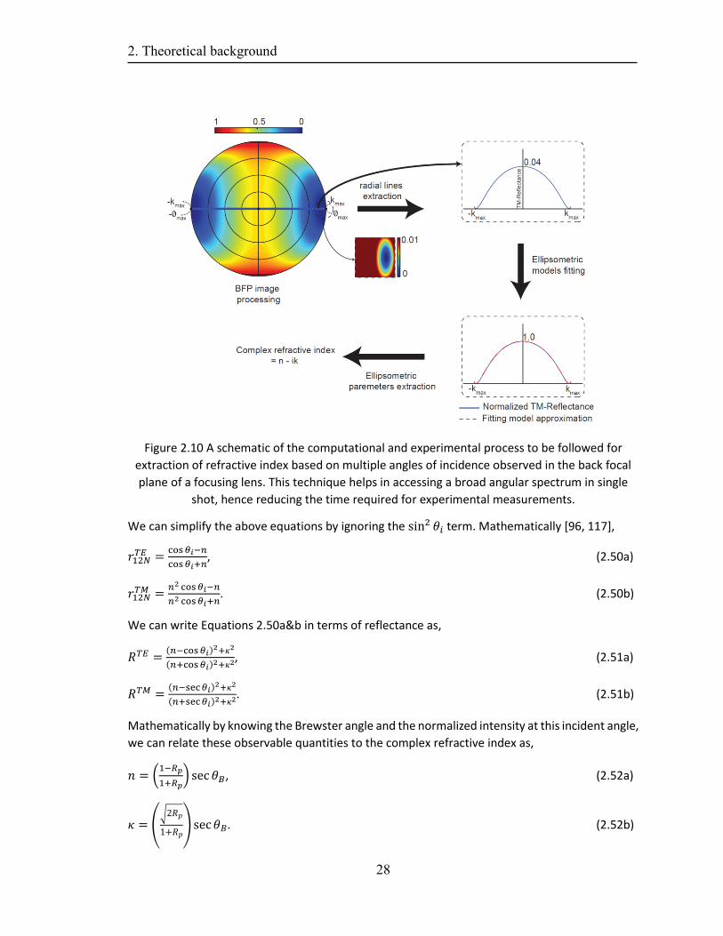
2. Theoretical background
28
Figure 2.10 A schematic of the computational and experimental process to be followed for
extraction of refractive index based on multiple angles of incidence observed in the back focal
plane of a focusing lens. This technique helps in accessing a broad angular spectrum in single
shot, hence reducing the time required for experimental measurements.
We can simplify the above equations by ignoring the sin2 𝜃𝑖 term. Mathematically [96, 117],
𝑟12𝑁𝑇𝐸 =
cos𝜃𝑖−𝑛
cos𝜃𝑖+𝑛, (2.50a)
𝑟12𝑁𝑇𝑀 =
𝑛2 cos𝜃𝑖−𝑛
𝑛2 cos𝜃𝑖+𝑛. (2.50b)
We can write Equations 2.50a&b in terms of reflectance as,
𝑅𝑇𝐸 =(𝑛−cos𝜃𝑖)
2+𝜅2
(𝑛+cos𝜃𝑖)2+𝜅2, (2.51a)
𝑅𝑇𝑀 =(𝑛−sec𝜃𝑖)
2+𝜅2
(𝑛+sec𝜃𝑖)2+𝜅2. (2.51b)
Mathematically by knowing the Brewster angle and the normalized intensity at this incident angle,
we can relate these observable quantities to the complex refractive index as,
𝑛 = (1−𝑅𝑝
1+𝑅𝑝) sec 𝜃𝐵, (2.52a)
𝜅 = (√2𝑅𝑝
1+𝑅𝑝) sec𝜃𝐵. (2.52b)
2. Theoretical background
29
Where, 𝜃𝐵 is the Brewster angle and 𝑅𝑝 is the related reflected intensity. As shown in equations
2.29a&b, the presence of cos 𝜃𝑖 and sec𝜃𝑖 in TE/TM-equations describe a diverging/converging
reflectance with increasing angles, which would be a crucial parameter for fitting model of these
equations. Additionally, we normalize Equations 2.29a&b for reflectance at normal incidence,
𝑅𝑁𝑇𝐸 =
(𝑛−cos𝜃𝑖)2+𝜅2
(𝑛−cos𝜃𝑖)2+𝜅2 ×
(𝑛+1)2+𝜅2
(𝑛−1)2+𝜅2, (2.53a)
𝑅𝑁𝑇𝑀 =
(𝑛−sec𝜃𝑖)2+𝑘2
(𝑛−sec𝜃𝑖)2+𝜅2 ×
(𝑛+1)2+𝜅2
(𝑛−1)2+𝜅2. (2.53b)
In some studies, above mentioned equations have been rigorously solved to find unique solutions
for real and imaginary part of refractive index or permittivity using a goniometric (moving parts)
setup [117].
We propose a single-shot method which combines high NA focusing lens-based ellipsometry
previously used for extracting only real part of refractive index [113] with the equations 2.53a&b
to extract complex refractive index as shown in Figure 2.10. By recording the back focal plane
(defined by 𝜃,Φ or 𝑘𝑥, 𝑘𝑦) of focusing objective in reflection, we can gather angularly resolved
reflectance (𝑅𝑁𝑇𝐸 , 𝑅𝑁
𝑇𝑀). This can be done by appropriately placing a lens in the reflection arm.
Since we acquired normalized reflectance (𝑅𝑁𝑇𝐸 , 𝑅𝑁
𝑇𝑀) from experimental measurements, we
apply nonlinear least square fitting method on equations 2.49a&b and 2.53a&b to extract the
unknown in equations; complex refractive index [123, 124]. Further details on experimental and
computational setup and evaluation would be discussed in section 3.2.6 and 3.3.4. Due to high
NA focusing objective we achieve focal spot in the order of wavelength of incident light, which
provides way lower spatial resolution as compared to existing commercial ellipsometer solutions
(tens of microns).
In the next chapter we will use the theoretical consideration and experimental techniques
(discussed in this chapter briefly) about polarized light matter-interaction to investigate novel
artificial material. We will discuss, an in-house built experimental setup to perform polarimetric
analysis (with high spatial resolution) of novel orthorhombic form of carbon (carbon flakes)
intercalated with bimetal (Au-Ag) nanoclusters. Later we will apply single-shot high NA objective
MAI Ellipsometry on said structure for complex refractive index retrieval.
In Chapter 4, expanding onto the concept of optical properties of a medium, we will study
diffraction assisted chiral scattering in 2D metasurfaces. There we will study intriguing optical
phenomenon (asymmetric transmission) as a result of carefully designing the shape and
orientation of individual building blocks of metasurfaces. Later, we will perform experimental
investigation of metasurfaces based on techniques mentioned briefly here and in Chapter 3 to
compare with simulation results.

3. 3D self-assembled carbon-metal hybrid structure
In this chapter we are going to discuss novel 3D self-assembled hybrid carbon-bimetal (Au-Ag)
structures, also referred to as carbon flakes [14, 15, 22-24]. The carbon flakes were discovered
and produced at the Institute of Chemistry of St. Petersburg State University and the optical
characterization is part of this thesis. In the beginning of this chapter, we will talk about its
intriguing structure, which motivated us to understand its optical response. Later, we will discuss
the experimental schemes used to observe the optical properties of individual carbon flakes,
which are a few microns in lateral dimensions. We will analyze the optical response of these
carbon flakes and will try to merge our chemical, experimental, and computational knowledge to
build an understanding of the complex mechanism of self-assembled carbon flakes. We will also
discuss the effect of fabrication parameters on structural and optical properties. The work was
done in collaboration with specialized research groups from different parts of the world including
St. Petersburg State University, Russia and University of Ottawa, Canada.
Self-assembled metamaterials
Self-assembly, ubiquitous in nature, is an exciting and intriguing phenomenon based on the
arrangement of certain building blocks into order without any direct external guidance or control
[125-128]. Understanding the process dynamics in terms of chemical and physical transformation
is an emerging field and can help us in realizing the very fundamental question of life on earth.
Indeed, complex chemical systems and their respective self-organized growth and sustenance are
the key to this open question [129-131].
In physical chemistry, special chemical compounds also known as supramolecular complexes
(herein referred as SMC) can be transformed such that the individual constituents arrange
themselves into regular structures [132-135]. This process involves careful selection of individual
chemical building-block parameters (geometry, physical dimensions, and density to name few) to
control the self-assembly process. However, understanding the nature of morphological control
in self-assembly has remained a major question [136]. A complete morphological control of self-
assembly can obviously help in steering the overall geometry to the desired shape, whereby
getting a deeper understanding of kinetic and thermodynamic equilibrium within the structure.
Recently, many groups have looked into the possibility of organo-metallic complexes [134, 137-
140]. These nature-inspired self-assembled structures are a promising candidate for nanoparticle-
based drug delivery systems and organic electronics applications [138]. With the advancement in
technology and precise nanofabrication facilities, self-assembled metamaterials are an emerging
field combining the knowledge and expertise of multiple scientific fields [141-143]. A particularly
interesting category of such forms are centered on with intercalated metal nanoparticles [20, 21,
144-149]. Due to their hybrid organic-plasmonic properties, they are considered as promising
materials for optics, nanophotonics, electrocatalysis, organic electronics and sensing technologies
[150, 151]. In this context, exploiting different phases of carbon have naturally attracted
researchers to employ them for such cases. Covalent Organic Frameworks (COF), where
covalently bonded molecular structures of light elements (C, H, N, O), or Metal Organic
Frameworks (MOF), where metal clusters with organic ligands/linker structures assemble into
large crystalline units, address the concept of different perspectives and physical compositions
3. 3D self-assembled carbon-metal hybrid structure
31
[138, 152-155]. An important area of research regarding these self-assembly phenomenon is the
so-called crystallinity-stability-functionality trade-off, where the structure can rearrange itself
due to external stimuli (e.g. pressure, temperature, electric fields gradient) to stay in a
thermodynamically minimum crystal state [156]. In the context of carbon, new exotic phases were
predicted under external stimuli conditions [157]. Recently, orthorhombic phase of carbon was
theoretically predicted, with intriguing optical and structural properties [154, 158-161].
In the following, we discuss a case of orthorhombic form of carbon, fabricated by self-assembly
process using laser induced deposition (LID) process [23, 24, 149]. The process is centered on the
breakdown and, later, recrystallization of a certain SMC as a result of laser irradiation at a
substrate/solution interface. LID offers a high flexibility and controllability. The LID process leads
to controllable growth of organometallic self-assembled micron-sized structures on a substrate
surface caused by the self-organization of the SMC constituents as shown in Figure 3.1a&b. The
LID of the hybrid metal-carbon structures is a straight-forward and convenient procedure that
does not require intense laser irradiation or special equipment. In the purview of this thesis, we
discuss the implications of the LID process on certain bimetallic (Au-Ag)-alkynyl ligand based SMC,
which results in the formation of [22, 23, 25] or other shapes such as flakes [14] and flowers [18]
of tunable composition, depending on the chosen SMC and the solvent [22]. One noteworthy type
of structure resulting from this process are carbon flakes (as shown in Figure 3.1b), which are the
first reported orthorhombic form of carbon (sp2 hybridized) with embedded Au-Ag nanoclusters
[14]. For the sake of brevity, we will keep our discussion in this chapter limited to carbon flakes,
which were investigated for their intriguing optical properties and may find applications in nano-
optics and spectroscopy [14, 24, 26].
3.1 Fabrication of novel hybrid structures
In purview of this thesis, we will discuss the use of alkynyl-phosphine ( PPh2(C6H4)3PPh2 ) based
ligand, which, together with heterometallic Au-Ag compound (Au13Ag12(C2Ph)20) and fluoride (PF6)
ions, helps in forming an organo-metallic SMC [23, 137, 149, 162-164]. The synthesis and chemical
characterization process will be discussed in the next section.
Chemical synthesis and characterization
The preparation of the required SMC and the fabrication of carbon flakes was done by our
collaborators at St. Petersburg State University, Russia under the supervision of Professor Alina
Manshina [20, 22, 23, 165-167]. A solution of the heterometallic-alkynyl phosphine SMC
{Au13Ag12(C2Ph)20(PPh2(C6H4)3PPh2)3}{PF6}5 was prepared in acetophenone (Aldrich, analytically
grade purity) at a specified concentration[21, 148]. The SMC solution was then placed in a cuvette
and covered with an ITO coated glass substrate (TIX 005 series from TECHINSTRO, with a thickness
of 1.1 mm), so that it is in contact with SMC solution [14, 15, 24, 168], as shown in Figure 3.1a. A
light source was focused to the substrate-solution interface from the substrate side in a fixed
position. As a light source we used a collimated He-Cd laser beam (CW, λ = 325 nm, I = 0.5 W/cm2)
with a beam waist of 𝜔0~1𝑚𝑚. The specific wavelength selected for irradiation is chosen to
correspond to the absorption spectrum of the SMC. The exposure time to irradiation can be varied
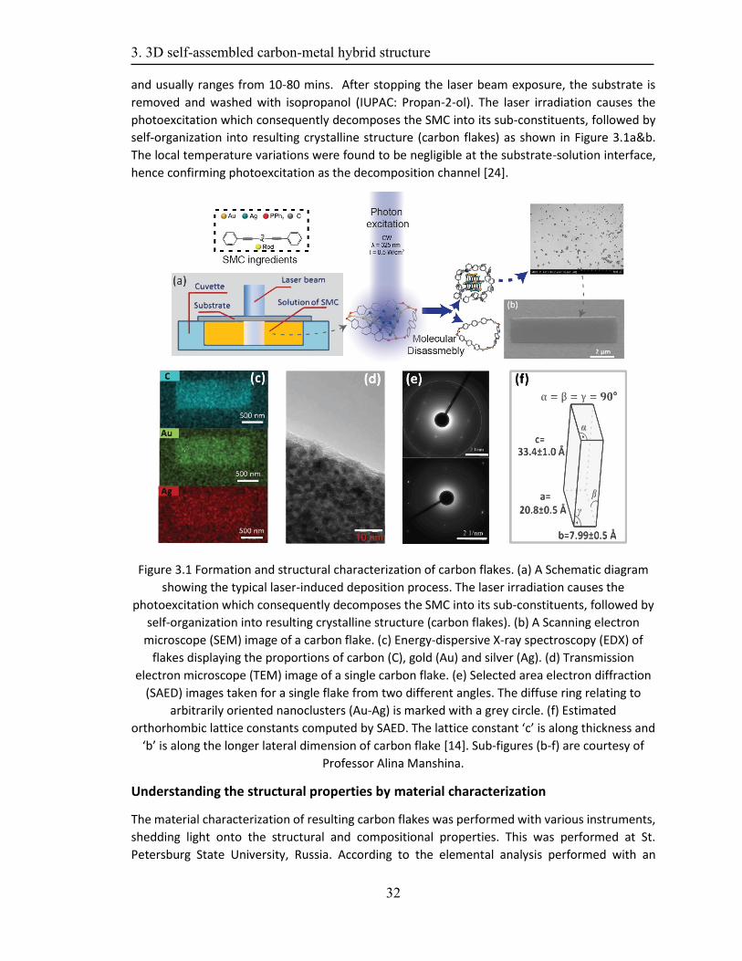
3. 3D self-assembled carbon-metal hybrid structure
32
and usually ranges from 10-80 mins. After stopping the laser beam exposure, the substrate is
removed and washed with isopropanol (IUPAC: Propan-2-ol). The laser irradiation causes the
photoexcitation which consequently decomposes the SMC into its sub-constituents, followed by
self-organization into resulting crystalline structure (carbon flakes) as shown in Figure 3.1a&b.
The local temperature variations were found to be negligible at the substrate-solution interface,
hence confirming photoexcitation as the decomposition channel [24].
Figure 3.1 Formation and structural characterization of carbon flakes. (a) A Schematic diagram
showing the typical laser-induced deposition process. The laser irradiation causes the
photoexcitation which consequently decomposes the SMC into its sub-constituents, followed by
self-organization into resulting crystalline structure (carbon flakes). (b) A Scanning electron
microscope (SEM) image of a carbon flake. (c) Energy-dispersive X-ray spectroscopy (EDX) of
flakes displaying the proportions of carbon (C), gold (Au) and silver (Ag). (d) Transmission
electron microscope (TEM) image of a single carbon flake. (e) Selected area electron diffraction
(SAED) images taken for a single flake from two different angles. The diffuse ring relating to
arbitrarily oriented nanoclusters (Au-Ag) is marked with a grey circle. (f) Estimated
orthorhombic lattice constants computed by SAED. The lattice constant ‘c’ is along thickness and
‘b’ is along the longer lateral dimension of carbon flake [14]. Sub-figures (b-f) are courtesy of
Professor Alina Manshina.
Understanding the structural properties by material characterization
The material characterization of resulting carbon flakes was performed with various instruments,
shedding light onto the structural and compositional properties. This was performed at St.
Petersburg State University, Russia. According to the elemental analysis performed with an
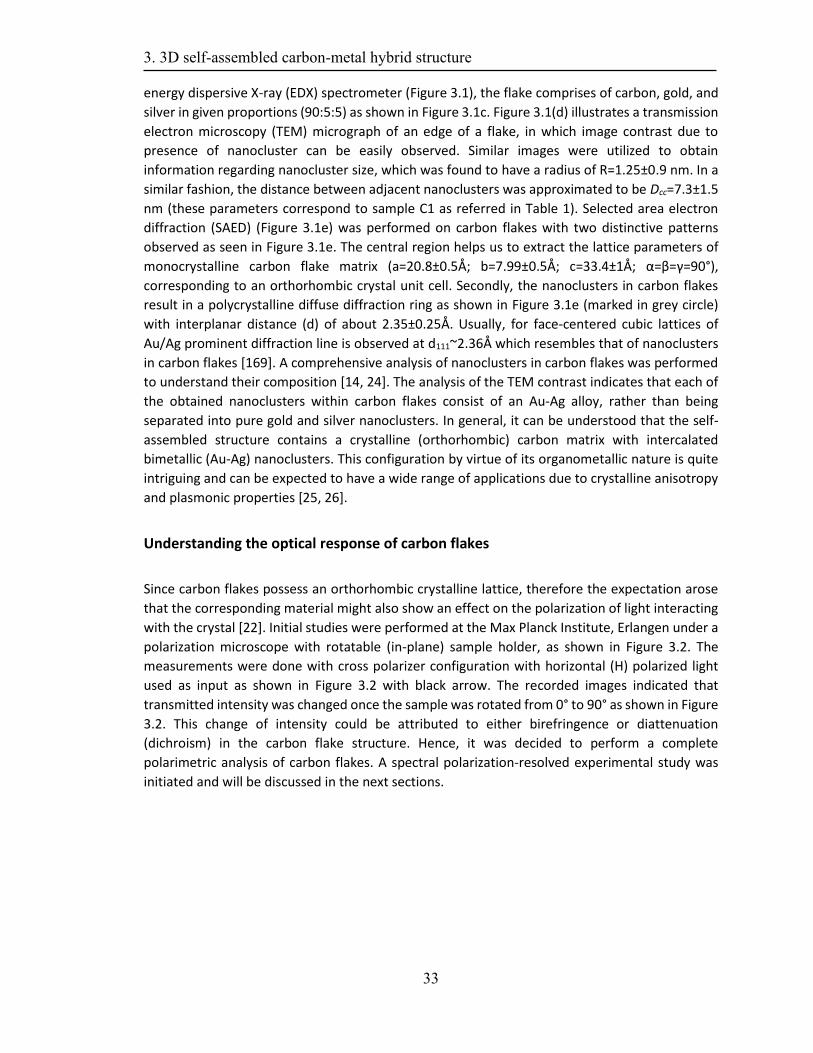
3. 3D self-assembled carbon-metal hybrid structure
33
energy dispersive X-ray (EDX) spectrometer (Figure 3.1), the flake comprises of carbon, gold, and
silver in given proportions (90:5:5) as shown in Figure 3.1c. Figure 3.1(d) illustrates a transmission
electron microscopy (TEM) micrograph of an edge of a flake, in which image contrast due to
presence of nanocluster can be easily observed. Similar images were utilized to obtain
information regarding nanocluster size, which was found to have a radius of R=1.25±0.9 nm. In a
similar fashion, the distance between adjacent nanoclusters was approximated to be Dcc=7.3±1.5
nm (these parameters correspond to sample C1 as referred in Table 1). Selected area electron
diffraction (SAED) (Figure 3.1e) was performed on carbon flakes with two distinctive patterns
observed as seen in Figure 3.1e. The central region helps us to extract the lattice parameters of
monocrystalline carbon flake matrix (a=20.8±0.5Å; b=7.99±0.5Å; c=33.4±1Å; α=β=γ=90°),
corresponding to an orthorhombic crystal unit cell. Secondly, the nanoclusters in carbon flakes
result in a polycrystalline diffuse diffraction ring as shown in Figure 3.1e (marked in grey circle)
with interplanar distance (d) of about 2.35±0.25Å. Usually, for face-centered cubic lattices of
Au/Ag prominent diffraction line is observed at d111~2.36Å which resembles that of nanoclusters
in carbon flakes [169]. A comprehensive analysis of nanoclusters in carbon flakes was performed
to understand their composition [14, 24]. The analysis of the TEM contrast indicates that each of
the obtained nanoclusters within carbon flakes consist of an Au-Ag alloy, rather than being
separated into pure gold and silver nanoclusters. In general, it can be understood that the self-
assembled structure contains a crystalline (orthorhombic) carbon matrix with intercalated
bimetallic (Au-Ag) nanoclusters. This configuration by virtue of its organometallic nature is quite
intriguing and can be expected to have a wide range of applications due to crystalline anisotropy
and plasmonic properties [25, 26].
Understanding the optical response of carbon flakes
Since carbon flakes possess an orthorhombic crystalline lattice, therefore the expectation arose
that the corresponding material might also show an effect on the polarization of light interacting
with the crystal [22]. Initial studies were performed at the Max Planck Institute, Erlangen under a
polarization microscope with rotatable (in-plane) sample holder, as shown in Figure 3.2. The
measurements were done with cross polarizer configuration with horizontal (H) polarized light
used as input as shown in Figure 3.2 with black arrow. The recorded images indicated that
transmitted intensity was changed once the sample was rotated from 0° to 90° as shown in Figure
3.2. This change of intensity could be attributed to either birefringence or diattenuation
(dichroism) in the carbon flake structure. Hence, it was decided to perform a complete
polarimetric analysis of carbon flakes. A spectral polarization-resolved experimental study was
initiated and will be discussed in the next sections.
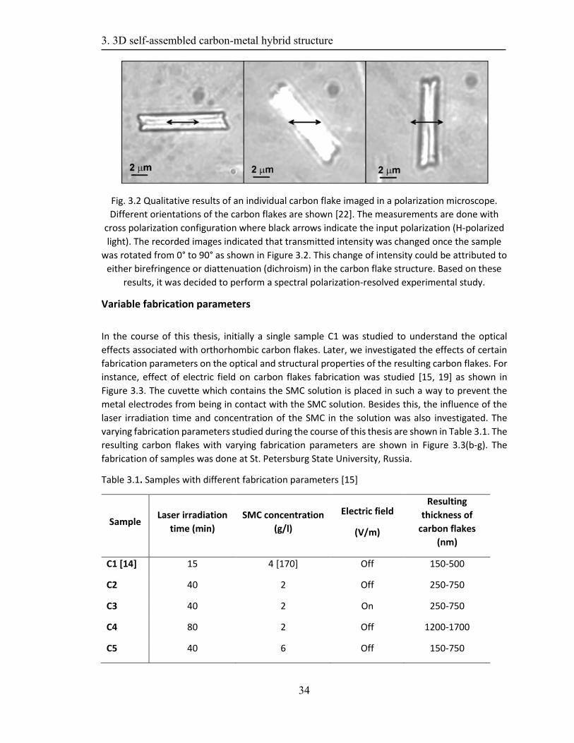
3. 3D self-assembled carbon-metal hybrid structure
34
Fig. 3.2 Qualitative results of an individual carbon flake imaged in a polarization microscope.
Different orientations of the carbon flakes are shown [22]. The measurements are done with
cross polarization configuration where black arrows indicate the input polarization (H-polarized
light). The recorded images indicated that transmitted intensity was changed once the sample
was rotated from 0° to 90° as shown in Figure 3.2. This change of intensity could be attributed to
either birefringence or diattenuation (dichroism) in the carbon flake structure. Based on these
results, it was decided to perform a spectral polarization-resolved experimental study.
Variable fabrication parameters
In the course of this thesis, initially a single sample C1 was studied to understand the optical
effects associated with orthorhombic carbon flakes. Later, we investigated the effects of certain
fabrication parameters on the optical and structural properties of the resulting carbon flakes. For
instance, effect of electric field on carbon flakes fabrication was studied [15, 19] as shown in
Figure 3.3. The cuvette which contains the SMC solution is placed in such a way to prevent the
metal electrodes from being in contact with the SMC solution. Besides this, the influence of the
laser irradiation time and concentration of the SMC in the solution was also investigated. The
varying fabrication parameters studied during the course of this thesis are shown in Table 3.1. The
resulting carbon flakes with varying fabrication parameters are shown in Figure 3.3(b-g). The
fabrication of samples was done at St. Petersburg State University, Russia.
Table 3.1. Samples with different fabrication parameters [15]
Sample Laser irradiation
time (min)
SMC concentration
(g/l)
Electric field
(V/m)
Resulting
thickness of
carbon flakes
(nm)
C1 [14] 15 4 [170] Off 150-500
C2 40 2 Off 250-750
C3 40 2 On 250-750
C4 80 2 Off 1200-1700
C5 40 6 Off 150-750
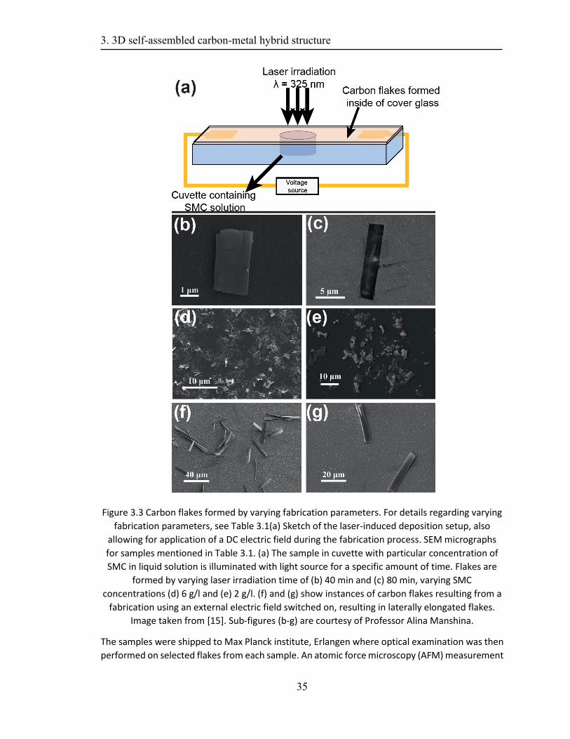
3. 3D self-assembled carbon-metal hybrid structure
35
Figure 3.3 Carbon flakes formed by varying fabrication parameters. For details regarding varying
fabrication parameters, see Table 3.1(a) Sketch of the laser-induced deposition setup, also
allowing for application of a DC electric field during the fabrication process. SEM micrographs
for samples mentioned in Table 3.1. (a) The sample in cuvette with particular concentration of
SMC in liquid solution is illuminated with light source for a specific amount of time. Flakes are
formed by varying laser irradiation time of (b) 40 min and (c) 80 min, varying SMC
concentrations (d) 6 g/l and (e) 2 g/l. (f) and (g) show instances of carbon flakes resulting from a
fabrication using an external electric field switched on, resulting in laterally elongated flakes.
Image taken from [15]. Sub-figures (b-g) are courtesy of Professor Alina Manshina.
The samples were shipped to Max Planck institute, Erlangen where optical examination was then
performed on selected flakes from each sample. An atomic force microscopy (AFM) measurement
3. 3D self-assembled carbon-metal hybrid structure
36
was performed on carbon flakes to estimate the thickness of carbon flakes with mean thickness
for various samples also mentioned in Table 3.1. The parameters shown in Table 3.1, affects the
decomposition rate that all together results in the variation of the flakes morphology/dimensions
and optical properties. As mentioned above, considering the unique nature of carbon flakes, it
would be interesting to understand its optical response. One of the immediate challenges with
direct polarimetric/ellipsometric measurements using commercially available solution is their
spatial resolution (in tens of microns). As already observed from the SEM micrographs (Figure
3.3b-g), the lateral dimensions of carbon flakes is in the order of few microns.
Hence, it was deemed necessary to develop a specialized technique to experimentally study
carbon flakes. A certain customized technique in this regard was developed and later modified at
the Max Planck Institute, Erlangen [14, 18]. The initial spectral measurements were performed by
Dr. Thomas Bauer, while later complete 2D scans and detailed study for carbon flake optical
properties and further experimental evaluation was performed by author. It helped us in
performing polarimetric analysis of carbon flakes at small scales (spatial resolution in the order of
incident wavelength). This technique will be discussed in detail in this chapter. Later we will apply
high NA objective MAI Ellipsometry on carbon flakes for complex refractive index retrieval.
3.2 Experimental setup
In this section, we describe our experimental methodology for retrieving the linear optical
properties of the examined carbon flakes. We analyze and extract linear optical parameters from
Müller matrix, such as birefringence, attenuation and diattenuation.
Microscopic Müller matrix measurement technique
We describe the various experimental and computational steps followed to extract optical
properties of examined carbon flakes mentioned in Figure 3.4. The microscopic Müller matrix
measurement technique merges the benefits of polarized light matter interaction with the back
focal plane (k-space / Fourier space) microscopy [29] and the usage of liquid crystal variable
retarders (LCVRs) to perform a comprehensive polarization analysis [14, 18, 30, 31]. The technique
is a combination of various experimental and computational steps that are performed for optical
properties extraction. The technique allows for doing a spatially resolved (with nanometer
resolution) far-field polarimetric analysis of micron-sized carbon flakes by performing a raster
scan of incident light beam over the examined structure. The usage of liquid crystal variable
retarders helps to avoid any moving optical elements in the analysis part of the setup [30]. In the
following subsections we will discuss various steps involved in this process and mentioned in
Figure 3.4.
Wavelength selection and polarization state generation
For the experimental method (see Figure 3.5a (i)) we use a broadband supercontinuum white light
laser source (NKT Photonics SuperK Extreme). For wavelength-selective filtering we use an
acousto-optical tunable filter (AOTF; Gooch & Housego AOTFnC-Vis / AOTF-UV).
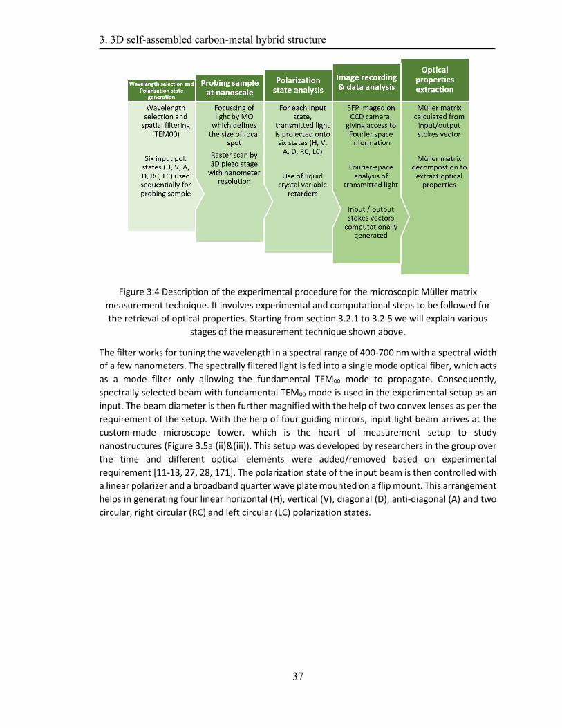
3. 3D self-assembled carbon-metal hybrid structure
37
Figure 3.4 Description of the experimental procedure for the microscopic Müller matrix
measurement technique. It involves experimental and computational steps to be followed for
the retrieval of optical properties. Starting from section 3.2.1 to 3.2.5 we will explain various
stages of the measurement technique shown above.
The filter works for tuning the wavelength in a spectral range of 400-700 nm with a spectral width
of a few nanometers. The spectrally filtered light is fed into a single mode optical fiber, which acts
as a mode filter only allowing the fundamental TEM00 mode to propagate. Consequently,
spectrally selected beam with fundamental TEM00 mode is used in the experimental setup as an
input. The beam diameter is then further magnified with the help of two convex lenses as per the
requirement of the setup. With the help of four guiding mirrors, input light beam arrives at the
custom-made microscope tower, which is the heart of measurement setup to study
nanostructures (Figure 3.5a (ii)&(iii)). This setup was developed by researchers in the group over
the time and different optical elements were added/removed based on experimental
requirement [11-13, 27, 28, 171]. The polarization state of the input beam is then controlled with
a linear polarizer and a broadband quarter wave plate mounted on a flip mount. This arrangement
helps in generating four linear horizontal (H), vertical (V), diagonal (D), anti-diagonal (A) and two
circular, right circular (RC) and left circular (LC) polarization states.
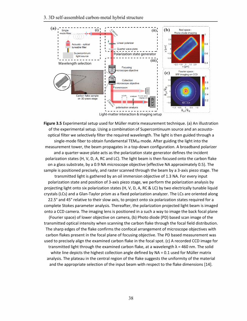
3. 3D self-assembled carbon-metal hybrid structure
38
Figure 3.5 Experimental setup used for Müller matrix measurement technique. (a) An illustration
of the experimental setup. Using a combination of Supercontinuum source and an acousto-
optical filter we selectively filter the required wavelength. The light is then guided through a
single-mode fiber to obtain fundamental TEM00 mode. After guiding the light into the
measurement tower, the beam propagates in a top-down configuration. A broadband polarizer
and a quarter-wave plate acts as the polarization state generator defines the incident
polarization states (H, V, D, A, RC and LC). The light beam is then focused onto the carbon flake
on a glass substrate, by a 0.9 NA microscope objective (effective NA approximately 0.5). The
sample is positioned precisely, and raster scanned through the beam by a 3-axis piezo stage. The
transmitted light is gathered by an oil immersion objective of 1.3 NA. For every input
polarization state and position of 3-axis piezo stage, we perform the polarization analysis by
projecting light onto six polarization states (H, V, D, A, RC & LC) by two electrically tunable liquid
crystals (LCs) and a Glan-Taylor prism as a fixed polarization analyzer. The LCs are oriented along
22.5° and 45° relative to their slow axis, to project onto six polarization states required for a
complete Stokes parameter analysis. Thereafter, the polarization projected light beam is imaged
onto a CCD camera. The imaging lens is positioned in a such a way to image the back focal plane
(Fourier space) of lower objective on camera, (b) Photo diode (PD) based scan image of the
transmitted optical intensity when scanning the carbon flake through the focal field distribution.
The sharp edges of the flake confirms the confocal arrangement of microscope objectives with
carbon flakes present in the focal plane of focusing objective. The PD based measurement was
used to precisely align the examined carbon flake in the focal spot. (c) A recorded CCD image for
transmitted light through the examined carbon flake, at a wavelength λ = 460 nm. The solid
white line depicts the highest collection angle defined by NA = 0.1 used for Müller matrix
analysis. The plateau in the central region of the flake suggests the uniformity of the material
and the appropriate selection of the input beam with respect to the flake dimensions [14].
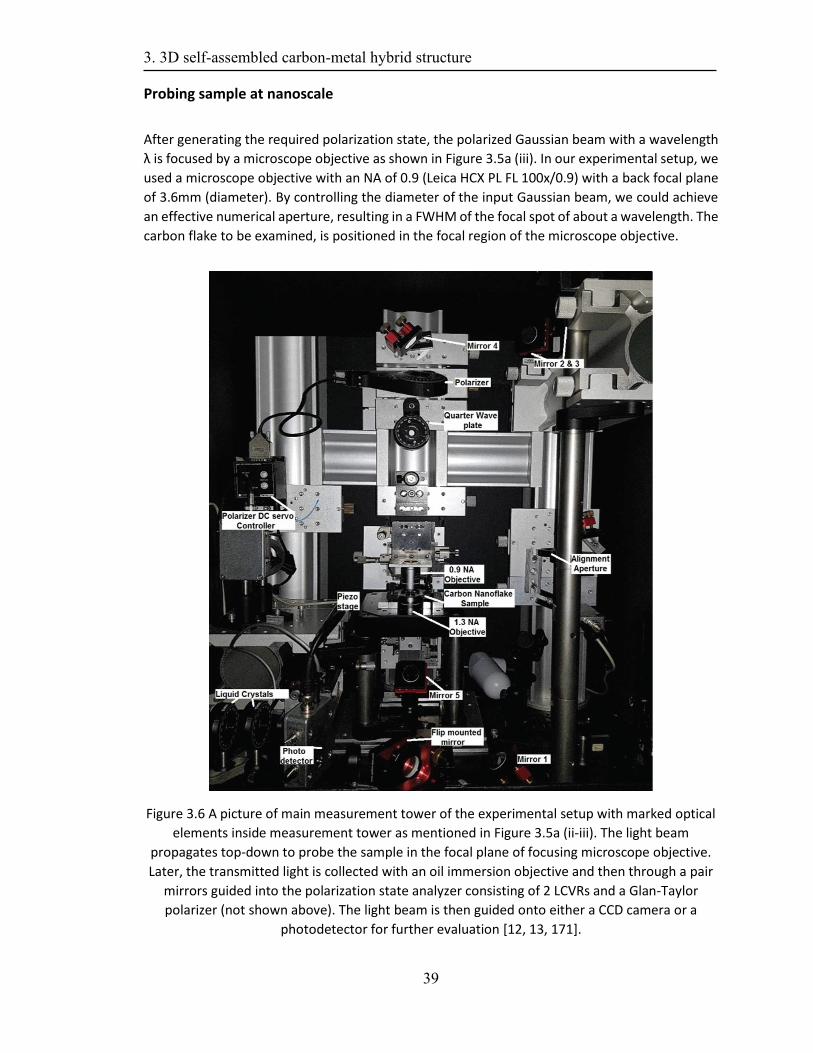
3. 3D self-assembled carbon-metal hybrid structure
39
Probing sample at nanoscale
After generating the required polarization state, the polarized Gaussian beam with a wavelength
λ is focused by a microscope objective as shown in Figure 3.5a (iii). In our experimental setup, we
used a microscope objective with an NA of 0.9 (Leica HCX PL FL 100x/0.9) with a back focal plane
of 3.6mm (diameter). By controlling the diameter of the input Gaussian beam, we could achieve
an effective numerical aperture, resulting in a FWHM of the focal spot of about a wavelength. The
carbon flake to be examined, is positioned in the focal region of the microscope objective.
Figure 3.6 A picture of main measurement tower of the experimental setup with marked optical
elements inside measurement tower as mentioned in Figure 3.5a (ii-iii). The light beam
propagates top-down to probe the sample in the focal plane of focusing microscope objective.
Later, the transmitted light is collected with an oil immersion objective and then through a pair
mirrors guided into the polarization state analyzer consisting of 2 LCVRs and a Glan-Taylor
polarizer (not shown above). The light beam is then guided onto either a CCD camera or a
photodetector for further evaluation [12, 13, 171].
3. 3D self-assembled carbon-metal hybrid structure
40
The small focal spot size (on the order of the wavelength) warrants that no edge effects contribute
to the measurements results obtained from the central region of the examined carbon flake. The
higher spatial resolution is one of the major advantages of our experimental setup as compared
to commercially available polarimetric systems. To perform a 2D scan, the carbon flake is
examined across the focal spot. This is done by mounting the carbon flake sample on a 3-axis
piezo scanning system (Physik Instrument P-525CD with an E-710 controller), which provides
lateral (x/y-axis) movement resolution of ~ 2nm and along propagation direction (z-axis) of
approximately 1 nm [11-13]. We use a custom designed sample holder which can be mounted
securely onto 3-axis piezo stage and firmly holds the carbon flakes sample. To ensure the lateral
levelling of the carbon flake sample, additionally two screws mounted on the sample holder helps
in controlling the tilt of the sample holder. A set of photo diodes are used in transmission,
reflection and as reference to align the sample/experimental setup and localize the examined
carbon flake within the lateral scan range of 3-axis piezo stage (x/y/z =200µm/200µm/20µm). In
order to evaluate the homogeneity of the carbon flakes under examination, we raster scanned
the carbon flakes individually across the beam and measured the transmitted intensity for each
position, resulting in the scanning image depicted in Figure 3.5b where a typical photodiode
readout for a carbon flake is shown. For each programmed scan position of the 3-axis piezo stage,
the transmitted light is collected by an oil-immersion microscope objective with an NA of 1.3
(Leica HCX PL FL 100x/1.3 Oil) in a large angular range. This lens has an aperture size of 5.2mm.
We image the back focal plane (BFP) of collection objective (see Figure 3.5c) onto a CCD-camera
(DMK23G618, Imaging Source) with 12 bit dynamic range to acquire the angular spectrum of the
transmitted light [172], using a single achromatic lens (f=300mm). In the recorded BFP images, we
computationally evaluate only the intensity in the angular cone (defined by NA) comparable to a
near-to-normal incidence. Thus, the effective angular range for Müller matrix analysis is preferred
to be constrained by a NA = 0.1, suggesting a half angle of around 5.5° (white solid circle in Figure
3.5c). The data shown is normalized for the transmission through the bare cover glass substrate.
As can be observed, the transmission decreases significantly when the focused incoming beam is
positioned on the examined carbon flake (Figure 3,5c). Here, we find a nearly constant plateau in
the central region of the flake, suggesting that the edge effects can be ignored for a central
positioning of the beam on carbon flake. Hence, the averaged polarization parameters of the
examined flake can be computed with statistical significance. We prepared differently polarized
six input beams as mentioned above, and determine their full Stokes polarization vector after the
transmission through the flake (𝐒𝑜𝑢𝑡) [85]. The end result is then equated to the transmission
through the cover glass substrate (𝐒𝑖𝑛) next to the flake for further data evaluation. A typical
custom-made microscope tower is shown in Figure 3.6 with the marked optical elements.
Polarization resolved analysis of optical structure
We perform a polarization projection of the light beam transmitted through the flake (or the bare
glass substrate for normalization purposes) to measure the respective Stokes vector. A
combination of two electrically tunable liquid crystal variable retarders (LCVRs; Thor Labs
LCC1115-A ) followed by a fixed polarization analyzer (Glan Taylor prism; Thor labs GT10-A) were
used for this purpose [173]. Aligning the slow-axis of the LCVRs cells at 22.5° and 45° with respect
to the preferred coordinate frame allows for determining the full Stokes vector by turning
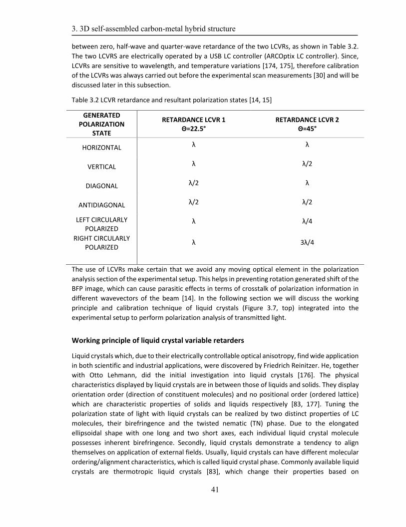
3. 3D self-assembled carbon-metal hybrid structure
41
between zero, half-wave and quarter-wave retardance of the two LCVRs, as shown in Table 3.2.
The two LCVRS are electrically operated by a USB LC controller (ARCOptix LC controller). Since,
LCVRs are sensitive to wavelength, and temperature variations [174, 175], therefore calibration
of the LCVRs was always carried out before the experimental scan measurements [30] and will be
discussed later in this subsection.
Table 3.2 LCVR retardance and resultant polarization states [14, 15]
GENERATED POLARIZATION
STATE
RETARDANCE LCVR 1 Θ=22.5°
RETARDANCE LCVR 2 Θ=45°
HORIZONTAL λ λ
VERTICAL λ λ/2
DIAGONAL λ/2 λ
ANTIDIAGONAL λ/2 λ/2
LEFT CIRCULARLY POLARIZED
λ λ/4
RIGHT CIRCULARLY POLARIZED
λ 3λ/4
The use of LCVRs make certain that we avoid any moving optical element in the polarization
analysis section of the experimental setup. This helps in preventing rotation generated shift of the
BFP image, which can cause parasitic effects in terms of crosstalk of polarization information in
different wavevectors of the beam [14]. In the following section we will discuss the working
principle and calibration technique of liquid crystals (Figure 3.7, top) integrated into the
experimental setup to perform polarization analysis of transmitted light.
Working principle of liquid crystal variable retarders
Liquid crystals which, due to their electrically controllable optical anisotropy, find wide application
in both scientific and industrial applications, were discovered by Friedrich Reinitzer. He, together
with Otto Lehmann, did the initial investigation into liquid crystals [176]. The physical
characteristics displayed by liquid crystals are in between those of liquids and solids. They display
orientation order (direction of constituent molecules) and no positional order (ordered lattice)
which are characteristic properties of solids and liquids respectively [83, 177]. Tuning the
polarization state of light with liquid crystals can be realized by two distinct properties of LC
molecules, their birefringence and the twisted nematic (TN) phase. Due to the elongated
ellipsoidal shape with one long and two short axes, each individual liquid crystal molecule
possesses inherent birefringence. Secondly, liquid crystals demonstrate a tendency to align
themselves on application of external fields. Usually, liquid crystals can have different molecular
ordering/alignment characteristics, which is called liquid crystal phase. Commonly available liquid
crystals are thermotropic liquid crystals [83], which change their properties based on
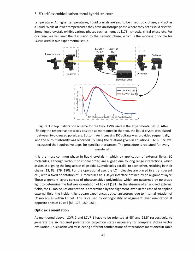
3. 3D self-assembled carbon-metal hybrid structure
42
temperature. At higher temperatures, liquid crystals are said to be in isotropic phase, and act as
a liquid. While at lower temperatures they have anisotropic phase where they act as solid crystals.
Some liquid crystals exhibit various phases such as nematic [178], smectic, chiral phase etc. For
our case, we will limit the discussion to the nematic phase, which is the working principle for
LCVRs used in our experimental setup.
Figure 3.7 Top: Calibration scheme for the two LCVRs used in the experimental setup. After
finding the respective optic axis position as mentioned in the text, the liquid crystal was placed
between two crossed polarizers. Bottom: An increasing DC voltage was provided sequentially,
and the output intensity was recorded. By using the relations given in Equations 3.1c & 3.2c, we
extracted the required voltages for specific retardances. The procedure is repeated for every
wavelength.
It is the most common phase in liquid crystals in which by application of external fields, LC
molecules, although without positional order, are aligned due to long range interactions, which
assists in aligning the long axis of ellipsoidal LC molecules parallel to each other, resulting in their
chains [13, 83, 179, 180]. For the operational use, the LC molecules are placed in a transparent
cell, with a fixed orientation of LC molecules at LC-layer interface defined by an alignment layer.
These alignment layers consist of photosensitive polyimides, which are patterned by polarized
light to determine the fast axis orientation of LC cell [181]. In the absence of an applied external
fields, the LC molecules orientation is determined by the alignment layer. In the case of an applied
external field, the incident light beam experiences optical anisotropy due to internal rotation of
LC molecules within LC cell. This is caused by orthogonality of alignment layer orientation at
opposite ends of LC cell [83, 173, 180, 181].
Optic axis orientation
As mentioned above, LCVR-2 and LCVR-1 have to be oriented at 45° and 22.5° respectively, to
generate the six required polarization projection states necessary for complete Stokes vector
evaluation. This is achieved by selecting different combinations of retardances mentioned in Table
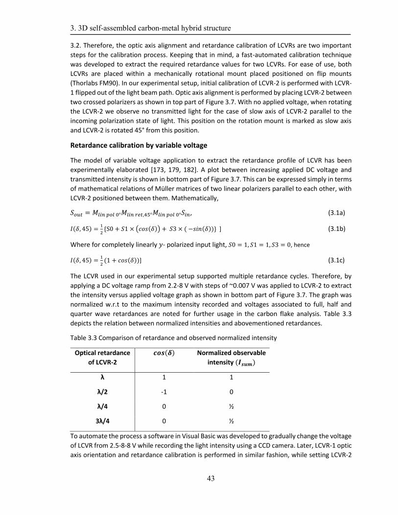
3. 3D self-assembled carbon-metal hybrid structure
43
3.2. Therefore, the optic axis alignment and retardance calibration of LCVRs are two important
steps for the calibration process. Keeping that in mind, a fast-automated calibration technique
was developed to extract the required retardance values for two LCVRs. For ease of use, both
LCVRs are placed within a mechanically rotational mount placed positioned on flip mounts
(Thorlabs FM90). In our experimental setup, initial calibration of LCVR-2 is performed with LCVR-
1 flipped out of the light beam path. Optic axis alignment is performed by placing LCVR-2 between
two crossed polarizers as shown in top part of Figure 3.7. With no applied voltage, when rotating
the LCVR-2 we observe no transmitted light for the case of slow axis of LCVR-2 parallel to the
incoming polarization state of light. This position on the rotation mount is marked as slow axis
and LCVR-2 is rotated 45° from this position.
Retardance calibration by variable voltage
The model of variable voltage application to extract the retardance profile of LCVR has been
experimentally elaborated [173, 179, 182]. A plot between increasing applied DC voltage and
transmitted intensity is shown in bottom part of Figure 3.7. This can be expressed simply in terms
of mathematical relations of Müller matrices of two linear polarizers parallel to each other, with
LCVR-2 positioned between them. Mathematically,
𝑆𝑜𝑢𝑡 = 𝑀𝑙𝑖𝑛 𝑝𝑜𝑙 0°𝑀𝑙𝑖𝑛 𝑟𝑒𝑡,45°𝑀𝑙𝑖𝑛 𝑝𝑜𝑙 0°𝑆𝑖𝑛, (3.1a)
𝐼(𝛿, 45) =1
2{S0 + 𝑆1 × (𝑐𝑜𝑠(𝛿)) + 𝑆3 × ( −𝑠𝑖𝑛(𝛿))} ] (3.1b)
Where for completely linearly 𝑦- polarized input light, 𝑆0 = 1, 𝑆1 = 1, 𝑆3 = 0, hence
𝐼(𝛿, 45) =1
2(1 + 𝑐𝑜𝑠(𝛿))] (3.1c)
The LCVR used in our experimental setup supported multiple retardance cycles. Therefore, by
applying a DC voltage ramp from 2.2-8 V with steps of ~0.007 V was applied to LCVR-2 to extract
the intensity versus applied voltage graph as shown in bottom part of Figure 3.7. The graph was
normalized w.r.t to the maximum intensity recorded and voltages associated to full, half and
quarter wave retardances are noted for further usage in the carbon flake analysis. Table 3.3
depicts the relation between normalized intensities and abovementioned retardances.
Table 3.3 Comparison of retardance and observed normalized intensity
Optical retardance
of LCVR-2
𝒄𝒐𝒔(𝜹) Normalized observable
intensity (𝑰𝒔𝒖𝒎)
λ 1 1
λ/2 -1 0
λ/4 0 ½
3λ/4 0 ½
To automate the process a software in Visual Basic was developed to gradually change the voltage
of LCVR from 2.5-8-8 V while recording the light intensity using a CCD camera. Later, LCVR-1 optic
axis orientation and retardance calibration is performed in similar fashion, while setting LCVR-2
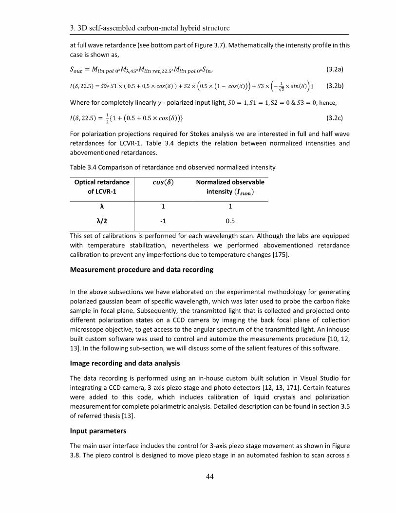
3. 3D self-assembled carbon-metal hybrid structure
44
at full wave retardance (see bottom part of Figure 3.7). Mathematically the intensity profile in this
case is shown as,
𝑆𝑜𝑢𝑡 = 𝑀𝑙𝑖𝑛 𝑝𝑜𝑙 0°𝑀λ,45°𝑀𝑙𝑖𝑛 𝑟𝑒𝑡,22.5°𝑀𝑙𝑖𝑛 𝑝𝑜𝑙 0°𝑆𝑖𝑛, (3.2a)
𝐼(𝛿, 22.5) = S0+ 𝑆1 × ( 0.5 + 0,5 × 𝑐𝑜𝑠(𝛿) ) + 𝑆2 × (0.5 × (1 − 𝑐𝑜𝑠(𝛿))) + 𝑆3 × (−1
√2× 𝑠𝑖𝑛(𝛿)) ] (3.2b)
Where for completely linearly y - polarized input light, 𝑆0 = 1, 𝑆1 = 1, S2 = 0 & 𝑆3 = 0, hence,
𝐼(𝛿, 22.5) = 1
2{1 + (0.5 + 0.5 × 𝑐𝑜𝑠(𝛿))} (3.2c)
For polarization projections required for Stokes analysis we are interested in full and half wave
retardances for LCVR-1. Table 3.4 depicts the relation between normalized intensities and
abovementioned retardances.
Table 3.4 Comparison of retardance and observed normalized intensity
Optical retardance
of LCVR-1
𝒄𝒐𝒔(𝜹) Normalized observable
intensity (𝑰𝒔𝒖𝒎)
λ 1 1
λ/2 -1 0.5
This set of calibrations is performed for each wavelength scan. Although the labs are equipped
with temperature stabilization, nevertheless we performed abovementioned retardance
calibration to prevent any imperfections due to temperature changes [175].
Measurement procedure and data recording
In the above subsections we have elaborated on the experimental methodology for generating
polarized gaussian beam of specific wavelength, which was later used to probe the carbon flake
sample in focal plane. Subsequently, the transmitted light that is collected and projected onto
different polarization states on a CCD camera by imaging the back focal plane of collection
microscope objective, to get access to the angular spectrum of the transmitted light. An inhouse
built custom software was used to control and automize the measurements procedure [10, 12,
13]. In the following sub-section, we will discuss some of the salient features of this software.
Image recording and data analysis
The data recording is performed using an in-house custom built solution in Visual Studio for
integrating a CCD camera, 3-axis piezo stage and photo detectors [12, 13, 171]. Certain features
were added to this code, which includes calibration of liquid crystals and polarization
measurement for complete polarimetric analysis. Detailed description can be found in section 3.5
of referred thesis [13].
Input parameters
The main user interface includes the control for 3-axis piezo stage movement as shown in Figure
3.8. The piezo control is designed to move piezo stage in an automated fashion to scan across a
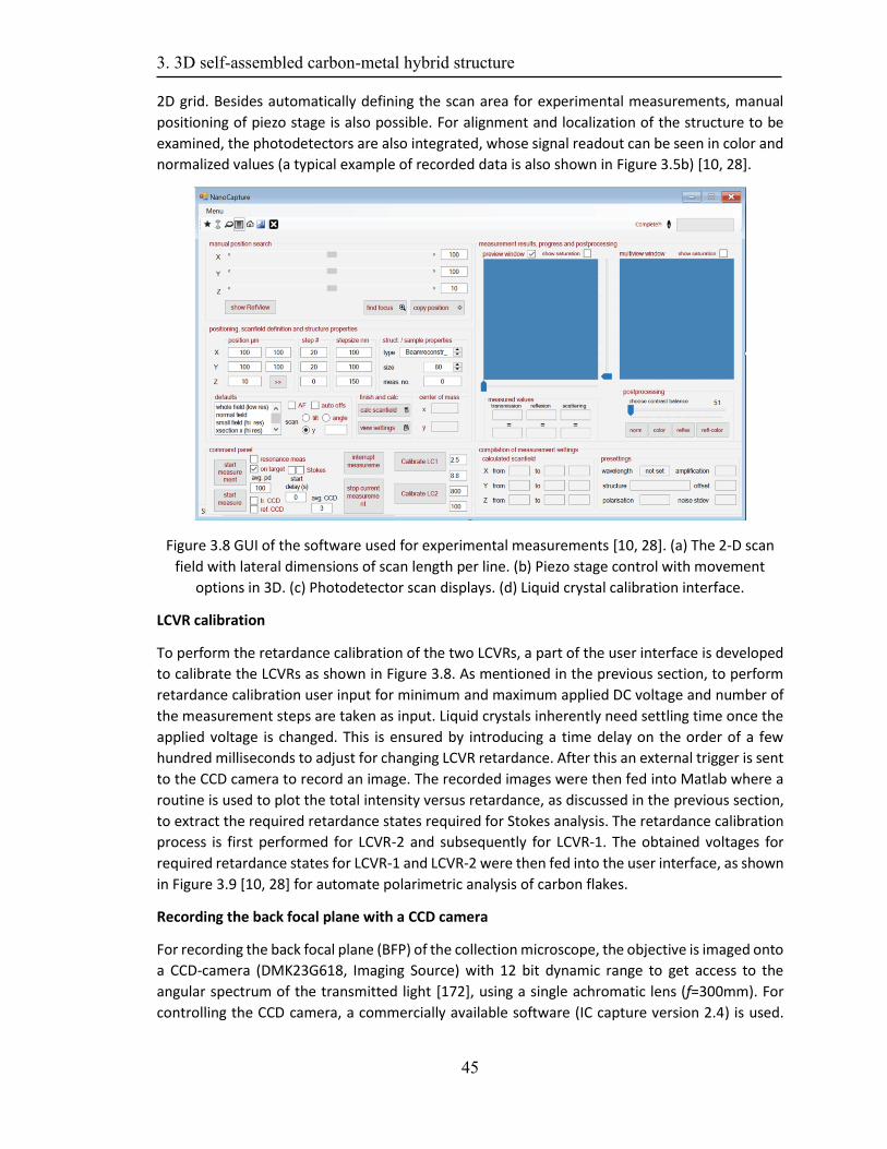
3. 3D self-assembled carbon-metal hybrid structure
45
2D grid. Besides automatically defining the scan area for experimental measurements, manual
positioning of piezo stage is also possible. For alignment and localization of the structure to be
examined, the photodetectors are also integrated, whose signal readout can be seen in color and
normalized values (a typical example of recorded data is also shown in Figure 3.5b) [10, 28].
Figure 3.8 GUI of the software used for experimental measurements [10, 28]. (a) The 2-D scan
field with lateral dimensions of scan length per line. (b) Piezo stage control with movement
options in 3D. (c) Photodetector scan displays. (d) Liquid crystal calibration interface.
LCVR calibration
To perform the retardance calibration of the two LCVRs, a part of the user interface is developed
to calibrate the LCVRs as shown in Figure 3.8. As mentioned in the previous section, to perform
retardance calibration user input for minimum and maximum applied DC voltage and number of
the measurement steps are taken as input. Liquid crystals inherently need settling time once the
applied voltage is changed. This is ensured by introducing a time delay on the order of a few
hundred milliseconds to adjust for changing LCVR retardance. After this an external trigger is sent
to the CCD camera to record an image. The recorded images were then fed into Matlab where a
routine is used to plot the total intensity versus retardance, as discussed in the previous section,
to extract the required retardance states required for Stokes analysis. The retardance calibration
process is first performed for LCVR-2 and subsequently for LCVR-1. The obtained voltages for
required retardance states for LCVR-1 and LCVR-2 were then fed into the user interface, as shown
in Figure 3.9 [10, 28] for automate polarimetric analysis of carbon flakes.
Recording the back focal plane with a CCD camera
For recording the back focal plane (BFP) of the collection microscope, the objective is imaged onto
a CCD-camera (DMK23G618, Imaging Source) with 12 bit dynamic range to get access to the
angular spectrum of the transmitted light [172], using a single achromatic lens (f=300mm). For
controlling the CCD camera, a commercially available software (IC capture version 2.4) is used.
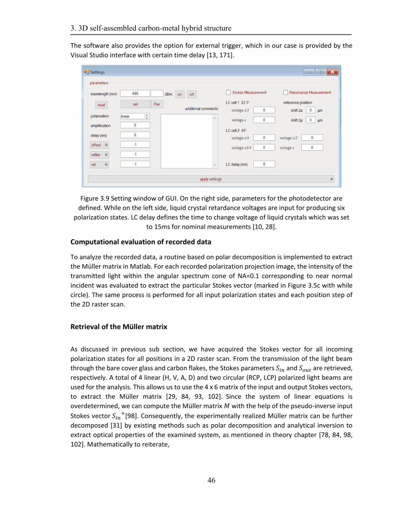
3. 3D self-assembled carbon-metal hybrid structure
46
The software also provides the option for external trigger, which in our case is provided by the
Visual Studio interface with certain time delay [13, 171].
Figure 3.9 Setting window of GUI. On the right side, parameters for the photodetector are
defined. While on the left side, liquid crystal retardance voltages are input for producing six
polarization states. LC delay defines the time to change voltage of liquid crystals which was set
to 15ms for nominal measurements [10, 28].
Computational evaluation of recorded data
To analyze the recorded data, a routine based on polar decomposition is implemented to extract
the Müller matrix in Matlab. For each recorded polarization projection image, the intensity of the
transmitted light within the angular spectrum cone of NA=0.1 corresponding to near normal
incident was evaluated to extract the particular Stokes vector (marked in Figure 3.5c with while
circle). The same process is performed for all input polarization states and each position step of
the 2D raster scan.
Retrieval of the Müller matrix
As discussed in previous sub section, we have acquired the Stokes vector for all incoming
polarization states for all positions in a 2D raster scan. From the transmission of the light beam
through the bare cover glass and carbon flakes, the Stokes parameters 𝑆𝑖𝑛 and 𝑆𝑜𝑢𝑡 are retrieved,
respectively. A total of 4 linear (H, V, A, D) and two circular (RCP, LCP) polarized light beams are
used for the analysis. This allows us to use the 4 x 6 matrix of the input and output Stokes vectors,
to extract the Müller matrix [29, 84, 93, 102]. Since the system of linear equations is
overdetermined, we can compute the Müller matrix 𝑀 with the help of the pseudo-inverse input
Stokes vector 𝑆𝑖𝑛+[98]. Consequently, the experimentally realized Müller matrix can be further
decomposed [31] by existing methods such as polar decomposition and analytical inversion to
extract optical properties of the examined system, as mentioned in theory chapter [78, 84, 98,
102]. Mathematically to reiterate,

3. 3D self-assembled carbon-metal hybrid structure
47
𝐒𝑜𝑢𝑡 = 𝑀𝐒𝑖𝑛 , 𝐒𝑜𝑢𝑡 = 𝑀∆𝑀𝑅𝑀𝐷𝐒𝑖𝑛, (3.3)
where 𝑀∆,𝑀𝑅 ,𝑀𝐷 represent the polar decomposition of a Müller matrix into individual
depolarizer, retarder and diattenuator matrices. These individual matrices can then further be
used to extract the required optical properties. Besides using polar decomposition, we extracted
the optical properties using analytical inversion method [29, 31, 84, 183]. Since the thickness of
flakes is usually limited to a few hundred nanometers and in very few cases to a micron, we
effectively have low retardance approximation, which makes estimates from polar decomposition
and analytical inversion approximately comparable [31].
Ellipsometric setup
The Müller matrix measurement technique adopted in transmission provides information mainly
regarding birefringence and dichroism. To access the direct information regarding refractive index
of the medium, we implemented a technique in the reflection arm of the setup explained above.
The setup was modified to accommodate for measurements in reflection in the back focal plane
and to generate different polarization states, which will be discussed below.
Preparing polarization states of the light beam
To prepare various linear and spatially structured light beams we use a combination of linear
polarizer and an electrically tunable spiral phase plate. For the results shown in this thesis, mainly
linearly polarized light was used. Use of spatially structured light is work in progress and in future
will greatly increase the benefits of current ellipsometry scheme. A discussion regarding spatially
structured light can be found in Appendix B to this thesis. we use a set of two beam splitters
(Thorlabs; PBS101) in orthogonal orientation (before focusing of light beam) to avoid any
polarization-dependent phase and amplitude variations [184]. This arrangement allows us to
collect the light beam in reflection without any polarization errors.
Probing the sample and recording the reflected signal
After generating the required polarization state, the polarized Gaussian beam with a wavelength
λ is focused by a microscope objective (Leica HCX PL FL 100x/0.9), as shown in Figure 3.10b&c. In
this case, the beam diameter of polarized light was made to match or be greater than the diameter
of entrance pupil of focusing objective (3.6mm). This would allow us to access the complete
angular spectrum offered by the objective. The planar sample to be examined is placed in the
focal plane similar to the arrangement mentioned in Section 3.2.2. This provides us with a focal
spot comparable to wavelength of light in visible frequency range. In the present experimental
setup, we examined samples in such a way to avoid internal reflections. This is done by positioning
the examined sample top surface, in the focal region of the focusing microscope objective and
avoiding multiple reflections by using a thicker substrate. Also, we examined samples with known
relatively larger thickness (evaluated by atomic force microscopy). By ensuring the precise
positioning of the focusing microscope objective, we can expect to have a collimated beam in the
reflection path as shown in Figure 3.10c. The back focal plane (BFP) of the focusing objective is
then imaged onto a CCD-camera (DMK23G618, Imaging Source). To get access to the angular
spectrum of the reflected light [172], we use a single achromatic lens (f=100mm).
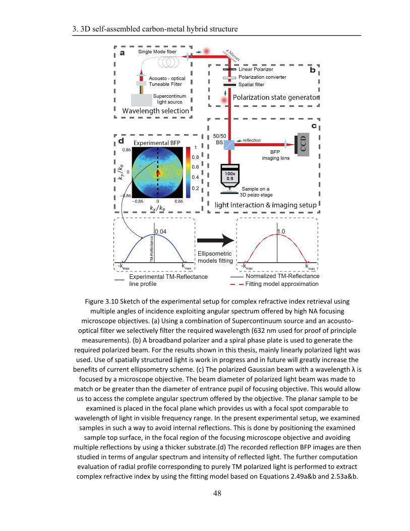
3. 3D self-assembled carbon-metal hybrid structure
48
Figure 3.10 Sketch of the experimental setup for complex refractive index retrieval using
multiple angles of incidence exploiting angular spectrum offered by high NA focusing
microscope objectives. (a) Using a combination of Supercontinuum source and an acousto-
optical filter we selectively filter the required wavelength (632 nm used for proof of principle
measurements). (b) A broadband polarizer and a spiral phase plate is used to generate the
required polarized beam. For the results shown in this thesis, mainly linearly polarized light was
used. Use of spatially structured light is work in progress and in future will greatly increase the
benefits of current ellipsometry scheme. (c) The polarized Gaussian beam with a wavelength λ is
focused by a microscope objective. The beam diameter of polarized light beam was made to
match or be greater than the diameter of entrance pupil of focusing objective. This would allow
us to access the complete angular spectrum offered by the objective. The planar sample to be
examined is placed in the focal plane which provides us with a focal spot comparable to
wavelength of light in visible frequency range. In the present experimental setup, we examined
samples in such a way to avoid internal reflections. This is done by positioning the examined
sample top surface, in the focal region of the focusing microscope objective and avoiding
multiple reflections by using a thicker substrate.(d) The recorded reflection BFP images are then
studied in terms of angular spectrum and intensity of reflected light. The further computation
evaluation of radial profile corresponding to purely TM polarized light is performed to extract
complex refractive index by using the fitting model based on Equations 2.49a&b and 2.53a&b.
3. 3D self-assembled carbon-metal hybrid structure
49
Image extraction and analysis
The recorded reflection BFP images (Figure 3.10d) are then studied in terms of angular spectrum
and intensity of reflected light. In order to extract the reflected intensity profile from the surface,
we normalize it w.r.t the incident light beam. This is done by placing a flat mirror just above the
focusing objective, to reflect the input beam onto the CCD camera, to record the reference input
beam Gaussian profile. Further Image processing on the recorded image is performed in Matlab.
The respective reference image is then used to normalize the BFP image of reflected light from
the examined sample’s top surface as shown in lower left corner of Figure 3.10. We define the
center of the BFP image as normal incident wavenumber (𝑘𝑥, 𝑘𝑦 = 0). The sharp edge of entrance
pupil of the focusing objective, observed in BFP image, acts as the basis for image segmentation
or defining maximum wavenumber (𝑘𝑚𝑎𝑥). As shown in bottom part of Figure 3.10, this radial
line, from the center 𝑘x/y = 0 to the outer edge, corresponds to the increasing wavenumber
𝑘𝑚𝑎𝑥. Once 𝑘x/y = 0 & 𝑘𝑚𝑎𝑥are defined, each pixel within the cropped circular BFP region can
be associated with Fourier coordinates (𝑘𝑥, 𝑘𝑦). A routine was then implemented to extract radial
(from -𝑘𝑚𝑎𝑥x to 𝑘𝑚𝑎𝑥) line segments along specified azimuthal angles (φ) of cropped circular BFP
image. These radial line profiles contain the reflected light intensity versus a transverse
wavenumber or varying incident angle data. By doing calibration measurements, the effective
𝑘𝑚𝑎𝑥=0.87 proportional to the maximum incidence angle of 60.25° was estimated for the current
measurement system and hence Fourier coordinates (𝑘𝑥 , 𝑘𝑦) were accordingly adjusted.
Computational model for ellipsometric analysis
The radial line profiles extracted are then fed as input to the fitting model developed for extracting
ellipsometric parameters. We use three different methods for extraction of complex refractive
index; firstly, direct estimation from reflected light intensity at Brewster angle using Equations
2.52a&b, approximate reflection calculations based on Equations 2.53a&b and full Fresnel
equations based on Fresnel coefficients mentioned in Equations 2.49a&b. As evident, The
nonlinear least square curve fitting function (lsqnonlin) in Matlab was used for second and third
case. The extracted radial line profiles are fitted accordingly to either TE or TM Fresnel equations
depending on incident polarization state of light. As evident, in case of first method, we use the
minimum intensity (for dielectric this is zero but for absorbing materials it is non-zero) at Brewster
angle, to approximate the complex refractive index [117]. As discussed, in our experimental setup,
the angle of incidence is limited by NA of the microscope objective. Hence, we can expect that for
materials, for which Brewster angle occurs above 60°, we will not be able to observe the
respective minima, which can lead to wrong approximations.
On the other hand, fitting models (based on Equation 2.49a&b and 2.53a&b) still can provide good
estimates, as will be discussed in the results section. This shows the two prong advantage of our
technique over previous results [113] for high AN objective MAI ellipsometry; complex refractive
index retrieval and because of fitting function we are not dependent on single point based
estimations. We perform experimental measurement on surfaces such as glass (isotropic), lithium
niobate (uniaxial) α-silicon (absorbing) for which ellipsometric data can be found in literature.
Later, we will test this scheme on the carbon flake to extract a preliminary estimate of complex
refractive index. The mapping of Fourier coordinates (𝑘𝑥 , 𝑘𝑦) to the specific pixels within circularly
cropped BFP images was kept constant for all examined samples.
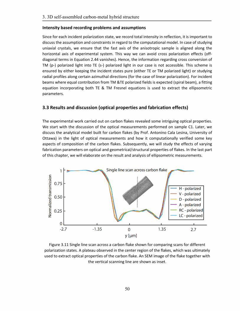
3. 3D self-assembled carbon-metal hybrid structure
50
Intensity based recording problems and assumptions
Since for each incident polarization state, we record total intensity in reflection, it is important to
discuss the assumption and constraints in regard to the computational model. In case of studying
uniaxial crystals, we ensure that the fast axis of the anisotropic sample is aligned along the
horizontal axis of experimental system. This way we can avoid cross polarization effects (off-
diagonal terms in Equation 2.44 vanishes). Hence, the information regarding cross conversion of
TM (p-) polarized light into TE (s-) polarized light in our case is not accessible. This scheme is
ensured by either keeping the incident states pure (either TE or TM polarized light) or studying
radial profiles along certain azimuthal directions (for the case of linear polarization). For incident
beams where equal contribution from TM &TE polarized fields is expected (spiral beam), a fitting
equation incorporating both TE & TM Fresnel equations is used to extract the ellipsometric
parameters.
3.3 Results and discussion (optical properties and fabrication effects)
The experimental work carried out on carbon flakes revealed some intriguing optical properties.
We start with the discussion of the optical measurements performed on sample C1. Later, we
discuss the analytical model built for carbon flakes (by Prof. Antonino Cala Lesina, University of
Ottawa) in the light of optical measurements and how it computationally verified some key
aspects of composition of the carbon flakes. Subsequently, we will study the effects of varying
fabrication parameters on optical and geometrical/structural properties of flakes. In the last part
of this chapter, we will elaborate on the result and analysis of ellipsometric measurements.
Figure 3.11 Single line scan across a carbon flake shown for comparing scans for different
polarization states. A plateau observed in the center region of the flakes, which was ultimately
used to extract optical properties of the carbon flake. An SEM image of the flake together with
the vertical scanning line are shown as inset.
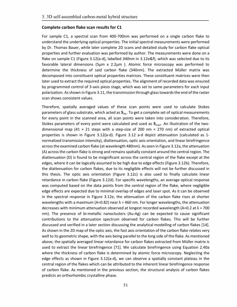
3. 3D self-assembled carbon-metal hybrid structure
51
Complete carbon flake scan results for C1
For sample C1, a spectral scan from 400-700nm was performed on a single carbon flake to
understand the underlying optical properties. The initial spectral measurements were performed
by Dr. Thomas Bauer, while later complete 2D scans and detailed study for carbon flake optical
properties and further evaluation was performed by author. The measurements were done on a
flake on sample C1 (Figure 3.12(a-d), labelled 340nm in 3.12e&f), which was selected due to its
favorable lateral dimensions (5µm x 2.2µm ). Atomic force microscopy was performed to
determine the thickness of said carbon flake (340nm). The extracted Müller matrix was
decomposed into constituent optical properties matrices. These constituent matrices were then
later used to extract the required optical properties. The alignment of recorded data was ensured
by programmed control of 3-axis piezo stage, which was set to same parameters for each input
polarization. As shown in Figure 3.11, the transmission through glass towards the end of the raster
scan shows consistent values.
Therefore, spatially averaged values of these scan points were used to calculate Stokes
parameters of glass substrate, which acted as 𝐒𝑖𝑛. To get a complete set of optical measurements
for every point in the scanned area, all scan points were taken into consideration. Therefore,
Stokes parameters of every point were calculated and used as 𝐒𝑜𝑢𝑡. An illustration of the two-
dimensional map (41 × 21 steps with a step-size of 200 nm × 270 nm) of extracted optical
properties is shown in Figure 3.12(a-d). Figure 3.12 a-d depict attenuation (calculated as 1-
normalized transmission intensity), diattenuation, optic axis orientation, and linear birefringence
across the examined carbon flake (at wavelength 480nm). As seen in Figure 3.12a, the attenuation
(A) across the carbon flake is strong and remains spatially constant around the central region. The
diattenuation (D) is found to be insignificant across the central region of the flake except at the
edges, where it can be logically assumed to be high due to edge effects (Figure 3.12b). Therefore,
the diattenuation for carbon flakes, due to its negligible effects will not be further discussed in
this thesis. The optic axis orientation (Figure 3.12c) is also used to finally calculate linear
retardance in carbon flake (Figure 3.12d). For specific wavelengths, an average optical response
was computed based on the data points from the central region of the flake, where negligible
edge effects are expected due to minimal overlap of edges and laser spot. As it can be observed
in the spectral response in Figure 3.12e, the attenuation of the carbon flake rises at shorter
wavelengths with a maximum (A=0.82) near λ = 460 nm. For longer wavelengths, the attenuation
decreases with minimum attenuation observed at longest recorded wavelength (A=0.2 at λ = 700
nm). The presence of bi-metallic nanoclusters (Au-Ag) can be expected to cause significant
contributions to the attenuation spectrum observed for carbon flakes. This will be further
discussed and verified in a later section discussing the analytical modelling of carbon flakes [14].
As shown in the 2D map of the optic axis, the fast axis orientation of the carbon flake relates very
well to its geometric shape, with the axis being parallel to the long side of the flake. As mentioned
above, the spatially averaged linear retardance for carbon flakes extracted from Müller matrix is
used to extract the linear birefringence [71]. We calculate birefringence using Equation 2.40a
where the thickness of carbon flake is determined by atomic force microscopy. Neglecting the
edge effects as shown in Figure 3.12(a-d), we can observe a spatially constant plateau in the
central region of the flakes which can be attributed to the inherent linear birefringence response
of carbon flake. As mentioned in the previous section, the structural analysis of carbon flakes
predicts an orthorhombic crystalline phase.
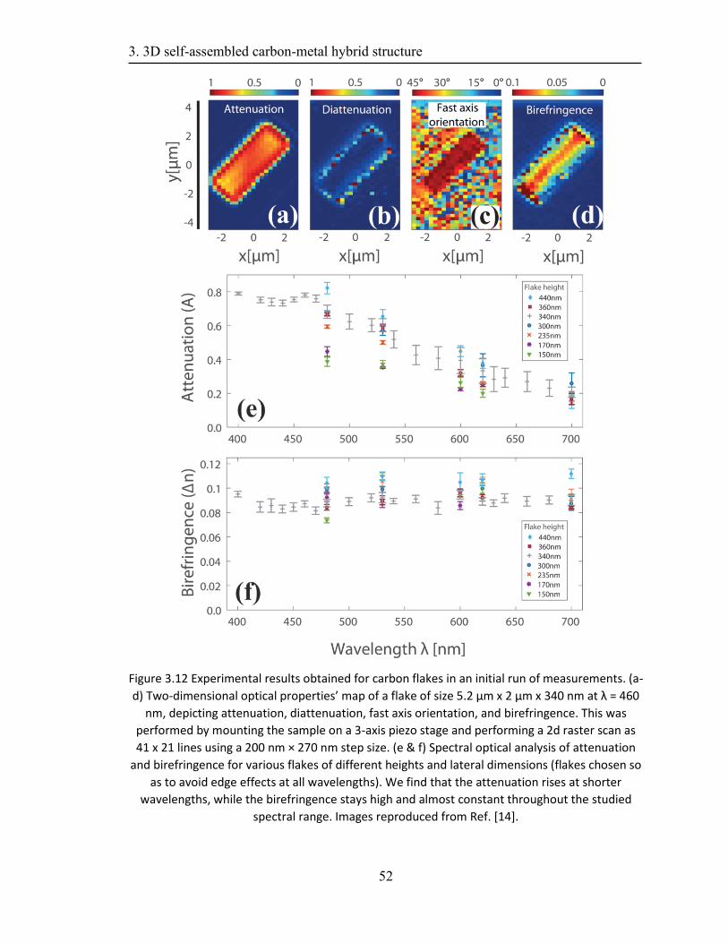
3. 3D self-assembled carbon-metal hybrid structure
52
Figure 3.12 Experimental results obtained for carbon flakes in an initial run of measurements. (a-
d) Two-dimensional optical properties’ map of a flake of size 5.2 μm x 2 μm x 340 nm at λ = 460
nm, depicting attenuation, diattenuation, fast axis orientation, and birefringence. This was
performed by mounting the sample on a 3-axis piezo stage and performing a 2d raster scan as
41 x 21 lines using a 200 nm × 270 nm step size. (e & f) Spectral optical analysis of attenuation
and birefringence for various flakes of different heights and lateral dimensions (flakes chosen so
as to avoid edge effects at all wavelengths). We find that the attenuation rises at shorter
wavelengths, while the birefringence stays high and almost constant throughout the studied
spectral range. Images reproduced from Ref. [14].
3. 3D self-assembled carbon-metal hybrid structure
53
Hence, we can relate the linear optical birefringence to the crystalline nature of carbon flake. In
order to further examine the birefringence, we perform a complete spectral analysis in the visible
spectrum (Figure 3.12f). Intriguingly, the linear birefringence is found to be almost constant (~0.09
±0.005) across the entire spectral range investigated. To verify uniformity of fabrication process
and the high birefringence, multiple flakes of varying thicknesses and lateral proportions (of at
least a few microns laterally to avoid edge effects) were studied (Figure 3.12 e&f). The evaluation
of those additional flakes was done only at some wavelengths but using the same experimental
scheme and assessment techniques. AFM scans of respective examined flakes were also
performed to approximate the height of individual carbon flake. Remarkably, all examined flakes
show similar values of birefringence (see Figure 3.12f), proving the consistency of the fabrication
process and confirming the presence of linear birefringence in crystalline carbon flakes.
Numerical modelling results and comparisons
To understand the optical response of carbon flakes, a computational model was built by
Professor Dr. Antonio Calà Lesina from the University of Ottawa, Canada. For the optical
properties present in carbon flakes two main contributions were considered: the bimetallic (Au-
Ag) nanoclusters and carbon matrix. Since the diameter of nanocluster is approximately similar to
the third dimension (c) of orthorhombic unit cell of carbon flake, it suggests that the nanoclusters
are intercalated in the carbon matrix as shown in Figure 3.13a. First part of computational study
was to model the nanoclusters present in carbon flakes. This was performed by emulating layers
of carbon sheets with intercalated nanoclusters (arranged in a face centered cubic (FCC) fashion
[14]) inspired by the first experimental study performed on carbon flake. The parameters such as
material composition of nanocluster, their effective diameter, spacing between two neighboring
nanoclusters and permittivity tensor of carbon sheets were kept variable. The initial analytical
model for nanoclusters was based on a modified Drude-Lorentz model to accommodate for
different proportions of bi-metallic particles (Au-Ag) [185] as shown in Figure 3.13ab. It was then
fitted to experimental data to find the proper approximations of parameters such as, nanocluster
inter-distance (Dcc), radius of nanoclusters (R),carbon matrix stretching factor (f), percentage
contributions of Au-Ag in nanoclusters and background refractive index (𝑛𝑏𝑎𝑐𝑘).These are briefly
discussed in Figure 3.13(b). For modelling the carbon layers, stretched graphene was first used in
the numerical model. This was accomplished by using experimental data for optical properties of
graphene obtained by spectroscopic ellipsometry [186]. This graphene model was modified by
changing its susceptibility (as discussed in Equation 2.23). The stretching factor facilitates the
modelling the carbon atoms within a layer, which is in essence equivalent to understanding
orthorhombic carbon crystalline structure. Keeping in consideration the orthorhombic crystalline
dimensions, we separate the layers of carbon by a distance of ~ 3.34 nm with background
refractive index as 𝑛𝑏𝑎𝑐𝑘 as mentioned above. The analytical model, as shown in Figure 3.13a, for
carbon flake was then simulated using the finite-difference time-domain (FDTD) approach [187].
Infinite lateral extension of modelled carbon flake is assumed based on periodic boundary
conditions in 𝑥 and 𝑦 direction, while light propagates in 𝑧 direction [188]. From the
computational model it was estimated that the average nanocluster inter-distance of 8nm
provides a solution closer to the experimental response. This is also verified by the TEM
measurements done on carbon flakes which estimates the nanocluster inter-distance Dcc=7.3±1.5
nm.
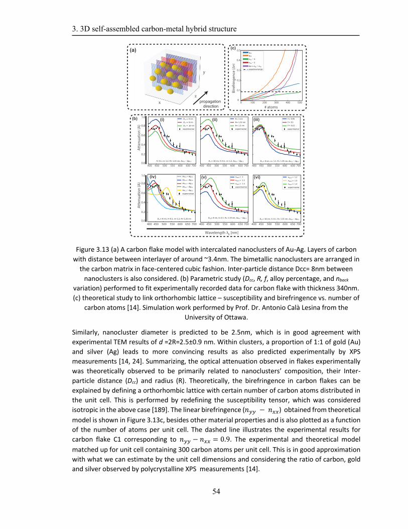
3. 3D self-assembled carbon-metal hybrid structure
54
Figure 3.13 (a) A carbon flake model with intercalated nanoclusters of Au-Ag. Layers of carbon
with distance between interlayer of around ~3.4nm. The bimetallic nanoclusters are arranged in
the carbon matrix in face-centered cubic fashion. Inter-particle distance Dcc= 8nm between
nanoclusters is also considered. (b) Parametric study (Dcc, R, f, alloy percentage, and nback
variation) performed to fit experimentally recorded data for carbon flake with thickness 340nm.
(c) theoretical study to link orthorhombic lattice – susceptibility and birefringence vs. number of
carbon atoms [14]. Simulation work performed by Prof. Dr. Antonio Calà Lesina from the
University of Ottawa.
Similarly, nanocluster diameter is predicted to be 2.5nm, which is in good agreement with
experimental TEM results of d =2R=2.5±0.9 nm. Within clusters, a proportion of 1:1 of gold (Au)
and silver (Ag) leads to more convincing results as also predicted experimentally by XPS
measurements [14, 24]. Summarizing, the optical attenuation observed in flakes experimentally
was theoretically observed to be primarily related to nanoclusters’ composition, their Inter-
particle distance (Dcc) and radius (R). Theoretically, the birefringence in carbon flakes can be
explained by defining a orthorhombic lattice with certain number of carbon atoms distributed in
the unit cell. This is performed by redefining the susceptibility tensor, which was considered
isotropic in the above case [189]. The linear birefringence (𝑛𝑦𝑦 − 𝑛𝑥𝑥) obtained from theoretical
model is shown in Figure 3.13c, besides other material properties and is also plotted as a function
of the number of atoms per unit cell. The dashed line illustrates the experimental results for
carbon flake C1 corresponding to 𝑛𝑦𝑦 − 𝑛𝑥𝑥 = 0.9. The experimental and theoretical model
matched up for unit cell containing 300 carbon atoms per unit cell. This is in good approximation
with what we can estimate by the unit cell dimensions and considering the ratio of carbon, gold
and silver observed by polycrystalline XPS measurements [14].
3. 3D self-assembled carbon-metal hybrid structure
55
Understanding control fabrication parameters and other optical properties
The carbon flake samples mentioned in Table 3.1, which represent different fabrication
parameters, were also experimentally investigated to understand the underlying effect of specific
fabrication parameters on the optical and structural properties of carbon flakes [15, 19]. To
extract the optical properties, we perform the experimental measurement and analysis in similar
fashion as mentioned above, for multiple flakes from samples mentioned in Table 3.1. We
examine the two optical properties of carbon flakes, i.e., attenuation and linear birefringence
across different carbon flakes. As discussed before, we evaluate the mean value for optical
property by studying the optical response in the central region of the flake where edge effects are
minimal. Besides, we perform an analysis on geometrical/structural properties of examined
carbon flakes.
Effect on the structural dimension of the carbon flakes
We used AFM to estimate the thickness of the examined flakes, while SEM was used to analyze
the lateral dimensions. SEM images of the examined flakes for variable fabrication parameters
are shown in Figure 3.3(b-g). Neglecting the slight variations in the flake’s dimensions, we can
deduce that the lateral dimensions of the examined carbon flakes are clearly correlated with
certain fabrication parameters. For instance, the SEM micrographs for DC-field switched off (see
Figure 3.3 b, e ) and for DC-field switched on (see Figure 3.3 f, g) show a visible difference in lateral
dimensions of fabricated carbon flakes. In these two scenarios (for sample C3 and C2 being E-field
‘on’ and ‘off’ respectively), other fabrication parameters were kept constant to single out the
resultant effect. It is pertinent to highlight that we observe an elongation in examined carbon
flakes along one lateral axis. The average size of carbon flakes, with electric field applied during
fabrication, reaches 40-60 µm in length and 5-10 µm in width (see Figure 3.3 f & g). These results
suggest that the lateral dimensions of flakes can be fine-tuned with the help of an applied electric
field. For the case of varying laser irradiation time, in case of C2 (C4) being 40 (80) mins
respectively, it was observed to directly impact the growth of the flakes, resulting in thicker flakes
observed by AFM measurements as shown in Table 3.1. Once more, we specifically consider the
two samples (C2 & C4) for which only laser irradiation time was changed while other fabrication
parameters were kept constant. AFM scans and SEM micrographs of the examined carbon flakes
show a direct relation. The thickness of carbon flakes was found to increase with increase in laser
irradiation time. Developing on this theory, we can assume that continued exposure to laser
irradiation helps produce requisite building block for the growth of flakes, by breakdown of SMC.
This in turn would pose a limit on the growth process which would be defined by the amount of
SMC aggregates present in the solution. It could be interesting to study this limiting phenomenon
in future studies. The attenuation of examined carbon flakes in both cases discussed above
remained unchanged, indicating uniformity in the fabrication process.
Effect of SMC concentration on attenuation
Here, we studied the effect of variable fabrication parameters on attenuation across the carbon
flakes. The attenuation across studied carbon flakes was normalized per 100nm to cater for the
varying thickness of the examined flakes (Figure 3.14).
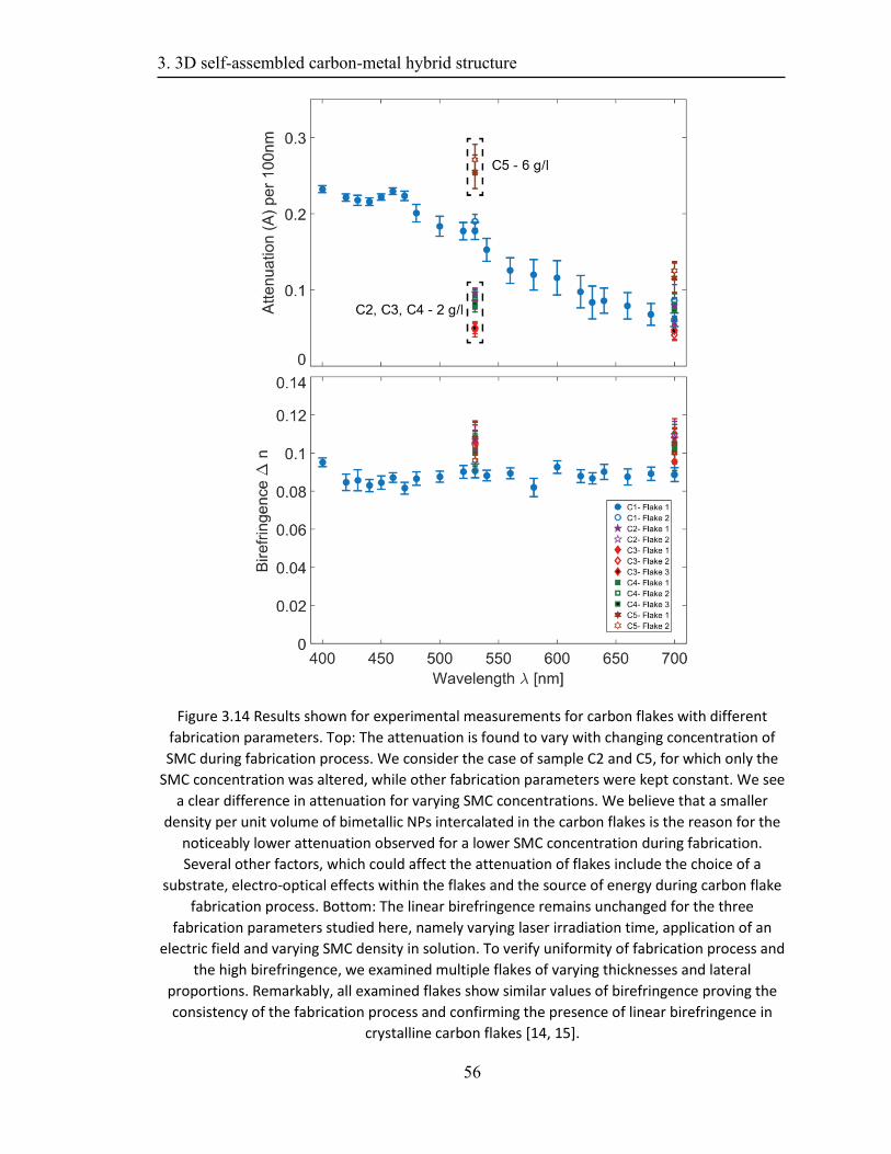
3. 3D self-assembled carbon-metal hybrid structure
56
Figure 3.14 Results shown for experimental measurements for carbon flakes with different
fabrication parameters. Top: The attenuation is found to vary with changing concentration of
SMC during fabrication process. We consider the case of sample C2 and C5, for which only the
SMC concentration was altered, while other fabrication parameters were kept constant. We see
a clear difference in attenuation for varying SMC concentrations. We believe that a smaller
density per unit volume of bimetallic NPs intercalated in the carbon flakes is the reason for the
noticeably lower attenuation observed for a lower SMC concentration during fabrication.
Several other factors, which could affect the attenuation of flakes include the choice of a
substrate, electro-optical effects within the flakes and the source of energy during carbon flake
fabrication process. Bottom: The linear birefringence remains unchanged for the three
fabrication parameters studied here, namely varying laser irradiation time, application of an
electric field and varying SMC density in solution. To verify uniformity of fabrication process and
the high birefringence, we examined multiple flakes of varying thicknesses and lateral
proportions. Remarkably, all examined flakes show similar values of birefringence proving the
consistency of the fabrication process and confirming the presence of linear birefringence in
crystalline carbon flakes [14, 15].
3. 3D self-assembled carbon-metal hybrid structure
57
We observe that by varying the SMC concentration in solution, the resulting attenuation across
the individual flakes can be altered. We consider the case of sample C2 and C5, for which other
fabrication parameters were kept constant and only the SMC concentration was changed. We
observe a clear difference in attenuation for varying SMC concentrations (Figure 3.14) [15].
In the theoretical modelling reviewed in our earlier study and discussed above [14, 15], we noticed
that the attenuation varies with the change in composition, diameter, and inter-particle distance
between adjacent bimetallic nanoclusters. Consequently, we believe that a smaller density per
unit volume of bimetallic NPs intercalated in the carbon flakes is the reason for the noticeably
lower attenuation observed for a lower SMC concentration during fabrication. Several other
factors, which could affect the attenuation of flakes include the choice of a substrate, electro-
optical effects within the flakes and the source of energy during carbon flake fabrication process
etc. [15].
Independence of linear birefringence of fabrication parameters
The linear birefringence remains unchanged for the three fabrication parameters studied here,
namely varying laser irradiation time, application of an electric field and varying SMC density in
solution (bottom part of Figure 3.14). To verify uniformity of fabrication process and the high
birefringence, we examined multiple flakes of varying thicknesses and lateral proportions (Figure
3.14). A similar measurement and assessment techniques were performed with AFM scans of
respective examined flakes to approximate the height of individual carbon flake. Remarkably, all
examined flakes show similar values of birefringence (see colored data points in Figure 3.12f),
proving the consistency of the fabrication process and confirming the presence of linear
birefringence in crystalline carbon flakes. This confirms the notion that the special crystalline
carbon phase causes the carbon flakes to exhibit linear birefringence.
Table 3.5. Variable fabrication parameters and their effect on carbon flakes [15]
Varied fabrication
parameter
Effect on optical properties of
carbon flakes
Effect on geometrical properties of
carbon flakes
Electric field on or off Optical properties remain
unchanged
Lateral elongation of flakes (with
field switched on)
Laser irradiation time Optical properties remain
unchanged
Increase in thickness with increasing
irradiation time
SMC density Increase in attenuation with
increasing SMC density
No observed effect on geometrical
properties
This also conforms with the analytical model built for carbon flakes, where linear birefringence
was a consequence of the orthorhombic crystalline phase. Summarizing the results of varying
fabrication parameters, we discuss them in the Table 3.5.
Circular birefringence of flakes
We observed in a recent analysis that carbon flakes could potentially also exhibit optical activity
(circular birefringence; CB). This could be attributed to intrinsic chirality of the alkynyl phosphine
ligand, which is part of SMC and contributes as a building block for carbon flakes.
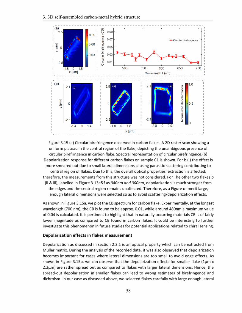
3. 3D self-assembled carbon-metal hybrid structure
58
Figure 3.15 (a) Circular birefringence observed in carbon flakes. A 2D raster scan showing a
uniform plateau in the central region of the flake, depicting the unambiguous presence of
circular birefringence in carbon flake. Spectral representation of circular birefringence.(b)
Depolarization response for different carbon flakes on sample C1 is shown. For b (i) the effect is
more smeared out due to small lateral dimensions causing parasitic scattering contributing to
central region of flakes. Due to this, the overall optical properties’ extraction is affected;
therefore, the measurements from this structure was not considered. For The other two flakes b
(ii & iii), labelled in Figure 3.13e&f as 340nm and 300nm, depolarization is much stronger from
the edges and the central region remains unaffected. Therefore, as a Figure of merit large,
enough lateral dimensions were selected so as to avoid scattering/depolarization effects.
As shown in Figure 3.15a, we plot the CB spectrum for carbon flake. Experimentally, at the longest
wavelength (700 nm), the CB is found to be approx. 0.01, while around 480nm a maximum value
of 0.04 is calculated. It is pertinent to highlight that in naturally occurring materials CB is of fairly
lower magnitude as compared to CB found in carbon flakes. It could be interesting to further
investigate this phenomenon in future studies for potential applications related to chiral sensing.
Depolarization effects in flakes measurement
Depolarization as discussed in section 2.3.1 is an optical property which can be extracted from
Müller matrix. During the analysis of the recorded data, it was also observed that depolarization
becomes important for cases where lateral dimensions are too small to avoid edge effects. As
shown in Figure 3.15b, we can observe that the depolarization effects for smaller flake (1µm x
2.2µm) are rather spread out as compared to flakes with larger lateral dimensions. Hence, the
spread-out depolarization in smaller flakes can lead to wrong estimates of birefringence and
dichroism. In our case as discussed above, we selected flakes carefully with large enough lateral
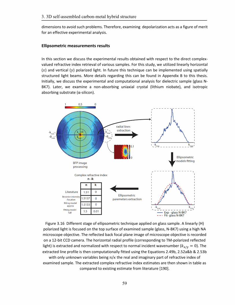
3. 3D self-assembled carbon-metal hybrid structure
59
dimensions to avoid such problems. Therefore, examining depolarization acts as a figure of merit
for an effective experimental analysis.
Ellipsometric measurements results
In this section we discuss the experimental results obtained with respect to the direct complex-
valued refractive index retrieval of various samples. For this study, we utilized linearly horizontal
(𝑥) and vertical (𝑦) polarized light. In future this technique can be implemented using spatially
structured light beams. More details regarding this can be found in Appendix B to this thesis.
Initially, we discuss the experimental and computational analysis for dielectric sample (glass N-
BK7). Later, we examine a non-absorbing uniaxial crystal (lithium niobate), and isotropic
absorbing substrate (α-silicon).
Figure 3.16 Different stage of ellipsometric technique applied on glass sample. A linearly (H)
polarized light is focused on the top surface of examined sample (glass, N-BK7) using a high NA
microscope objective. The reflected back focal plane image of microscope objective is recorded
on a 12-bit CCD camera. The horizontal radial profile (corresponding to TM-polarized reflected
light) is extracted and normalized with respect to normal incident wavenumber (𝑘x/y = 0). The
extracted line profile is then computationally fitted using the Equations 2.49b, 2.52a&b & 2.53b
with only unknown variables being 𝑛/𝜅 the real and imaginary part of refractive index of
examined sample. The extracted complex refractive index estimates are then shown in table as
compared to existing estimate from literature [190].
3. 3D self-assembled carbon-metal hybrid structure
60
Lastly, we present our preliminary experimental results for carbon flakes refractive index and
analyzed them in light of optical properties extracted by microscopic Müller matrix measurement
technique. All of the experimental results mentioned below were performed at a wavelength of
632nm.
Ellipsometric parameters for a dielectric: glass
We discuss first the case of glass (N-BK7) for ellipsometric parameters extraction. By following the
scheme mentioned in Section 3.2.6, we evaluate the BFP to computationally estimate the
refractive index. The measurement on glass also served as a reference for the ellipsometric system
and to understand the constraints or limitations in this regard. We use horizontal-polarized
incident light beam to probe the sample. The reflected back focal plane image of microscope
objective is recorded on a 12-bit CCD camera as shown in top right corner of Figure 3.16. We
extracted the line profile from BFP along the horizontal axis, where a pure TM reflected light is
expected as shown in top left corner of Figure 3.16. The spurious high intensity reflections near
normal incidence can be attributed to reflections from lower interface of cover glass. We used
three different methods for extraction of complex refractive index; full Fresnel equations based
on Fresnel coefficients mentioned in Equations 2.49b, direct estimation from reflected light
intensity at Brewster angle using Equations 2.52a&b and approximate reflection calculations
based on Equations 2.53b.
From the line profile and recorded BFP images (top left corner of Figure 3.16), we can clearly
observe the vanishing intensity expected at the Brewster angle for TM reflectance from glass (N-
BK7). The extracted line profile is then computationally fitted using the equations mentioned
above with only unknown variables being 𝑛/𝜅 the real and imaginary part of refractive index of
examined sample. The nonlinear least square curve fitting function (lsqnonlin) in Matlab was used
for this purpose. The extracted complex refractive index estimates are shown in lower left corner
in Figure 3.16 in a table as compared to existing estimate from literature [190]. The estimates are
in in good agreement with the expected refractive index of glass and assures us of the workability
of this scheme. The spurious reflections near normal incidence does not cause too much deviation
to our final complex refractive index estimates. This will be discussed in detail in our next
experimental case.
Ellipsometric parameters for uniaxial non-absorbent materials: Lithium Niobate
As a second case, we perform the ellipsometric measurement on a uniaxial crystal (Lithium
Niobate). In case of a uniaxial crystal, we expect two refractive indices (ordinary 𝑛𝑜/𝜅𝑜 and
extraordinary 𝑛𝑒/𝜅𝑒) along two principal axes of the crystal. In this regard, we studied a sample
of lithium niobate and followed the similar experimental procedure as adopted for glass. We use
horizontal-polarized incident light beam to probe the sample. The sample is aligned such that the
fast axis of lithium niobate sample points in the direction of incident polarized light (H-polarized)
to avoid retardance effects as discussed in section 3.2.6. The reflected back focal plane image of
microscope objective is recorded on a 12-bit CCD camera. We extracted the line profile from BFP
along the horizontal axis, where a pure TM reflected light is expected as shown in Figure top right
corner of 3.17. Due to spurious reflections, the central part of the BFP was removed and
subsequently fitting was performed as shown in Figure top left corner of 3.17. The extracted line
profile is then computationally fitted using the Equation 2.49b, 2.52a&b & 2.53b with only
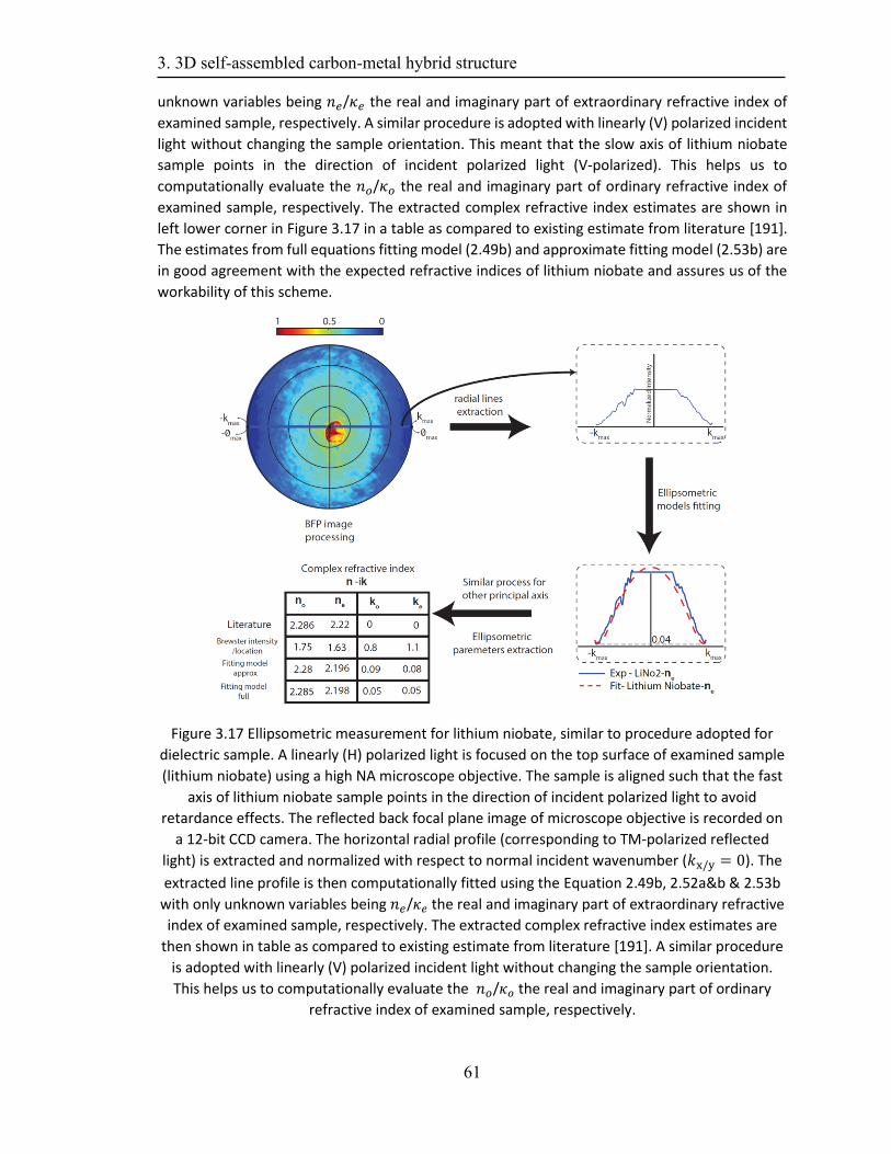
3. 3D self-assembled carbon-metal hybrid structure
61
unknown variables being 𝑛𝑒/𝜅𝑒 the real and imaginary part of extraordinary refractive index of
examined sample, respectively. A similar procedure is adopted with linearly (V) polarized incident
light without changing the sample orientation. This meant that the slow axis of lithium niobate
sample points in the direction of incident polarized light (V-polarized). This helps us to
computationally evaluate the 𝑛𝑜/𝜅𝑜 the real and imaginary part of ordinary refractive index of
examined sample, respectively. The extracted complex refractive index estimates are shown in
left lower corner in Figure 3.17 in a table as compared to existing estimate from literature [191].
The estimates from full equations fitting model (2.49b) and approximate fitting model (2.53b) are
in good agreement with the expected refractive indices of lithium niobate and assures us of the
workability of this scheme.
Figure 3.17 Ellipsometric measurement for lithium niobate, similar to procedure adopted for
dielectric sample. A linearly (H) polarized light is focused on the top surface of examined sample
(lithium niobate) using a high NA microscope objective. The sample is aligned such that the fast
axis of lithium niobate sample points in the direction of incident polarized light to avoid
retardance effects. The reflected back focal plane image of microscope objective is recorded on
a 12-bit CCD camera. The horizontal radial profile (corresponding to TM-polarized reflected
light) is extracted and normalized with respect to normal incident wavenumber (𝑘x/y = 0). The
extracted line profile is then computationally fitted using the Equation 2.49b, 2.52a&b & 2.53b
with only unknown variables being 𝑛𝑒/𝜅𝑒 the real and imaginary part of extraordinary refractive
index of examined sample, respectively. The extracted complex refractive index estimates are
then shown in table as compared to existing estimate from literature [191]. A similar procedure
is adopted with linearly (V) polarized incident light without changing the sample orientation.
This helps us to computationally evaluate the 𝑛𝑜/𝜅𝑜 the real and imaginary part of ordinary
refractive index of examined sample, respectively.
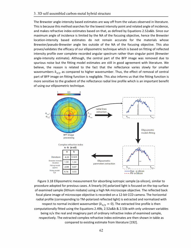
3. 3D self-assembled carbon-metal hybrid structure
62
The Brewster angle-intensity based estimates are way off from the values observed in literature.
This is because this method searches for the lowest intensity point and related angle of incidence,
and makes refractive index estimates based on that, as defined by Equations 2.52a&b. Since our
maximum angle of incidence is limited by the NA of the focusing objective, hence the Brewster
location-intensity based estimates do not remain accurate for the materials whose
Brewster/pseudo-Brewster angle lies outside of the NA of the focusing objective. This also
proves/validates the efficacy of our ellipsometric technique which is based on fitting of reflected
intensity profile over complete recorded angular spectrum rather than singular point (Brewster
angle-intensity estimate). Although, the central part of the BFP image was removed due to
spurious noise but the fitting model estimates are still in good agreement with literature. We
believe, the reason is related to the fact that the reflectance varies slowly for smaller
wavenumbers 𝑘x/y as compared to higher wavenumber. Thus, the effect of removal of central
part of BFP image on fitting function is negligible. This also informs us that the fitting function is
more sensitive to the gradient of the reflectance radial line profile which is an important benefit
of using our ellipsometric technique.
Figure 3.18 Ellipsometric measurement for absorbing isotropic sample (α-silicon), similar to
procedure adopted for previous cases. A linearly (H) polarized light is focused on the top surface
of examined sample (lithium niobate) using a high NA microscope objective. The reflected back
focal plane image of microscope objective is recorded on a 12-bit CCD camera. The horizontal
radial profile (corresponding to TM-polarized reflected light) is extracted and normalized with
respect to normal incident wavenumber (𝑘x/y = 0). The extracted line profile is then
computationally fitted using the Equations 2.49b, 2.52a&b & 2.53b with only unknown variables
being 𝑛/𝜅 the real and imaginary part of ordinary refractive index of examined sample,
respectively. The extracted complex refractive index estimates are then shown in table as
compared to existing estimate from literature [192].
3. 3D self-assembled carbon-metal hybrid structure
63
Ellipsometric parameters for absorbing isotropic materials.
Next, we consider the case of absorbing material. In this regard, we study a sample of α-silicon
substrate (Figure 3.18). We use horizontal-polarized incident light beam to probe the sample. The
reflected back focal plane image of microscope objective is recorded on a 12-bit CCD camera in
similar fashion as mentioned above. We extracted the line profile from BFP along the horizontal
axis, where a pure TM reflected light is expected as shown in Figure 3.17. The extracted line profile
is then computationally fitted using the Equation 2.49b, 2.52a&b & 2.53b with only unknown
variables being 𝑛/𝜅 the real and imaginary part of ordinary refractive index of examined sample,
respectively. The extracted complex refractive index estimates are shown in left lower corner in
Figure 3.17 in a table as compared to existing estimate from literature [192]. The estimates from
full equations fitting model (2.49b) is in good agreement with the expected refractive indices of
α-silicon (from literature) and assures us of the workability of our scheme. As expected, from the
refractive index of α-silicon, the Brewster angle lies outside the NA of microscope objective.
Therefore, Brewster angle-intensity based estimates (as defined by Equations 2.52a&b) are way
off from the values observed in literature. The approximate equations-based model also show
way off estimates. This can probably be attributed to noise and approximation of equations which
leads to bad estimated of refractive index.
Ellipsometric parameters for carbon flakes
As a next case, we measure a carbon flake in a similar fashion as mentioned above. These
measurements hence provide us with first principal approximations of the refractive index of
Carbon flake. We use horizontal-polarized incident light beam to probe the sample. The sample is
aligned such that the fast axis of individual carbon flake points in the direction of incident
polarized light (H-polarized) to avoid retardance effects as discussed in section 3.2.6. The reflected
back focal plane image of microscope objective is recorded on a 12-bit CCD camera in similar
fashion as abovementioned cases. We extracted the line profile from BFP along the horizontal
axis, where a pure TM reflected light is expected as shown in top right corner of Figure 3.17.
We used three similar methods for extraction of complex refractive index as above; full Fresnel
equations based on Fresnel coefficients mentioned in Equations 2.49b, direct estimation from
reflected light intensity at Brewster angle using Equations 2.52a&b and approximate reflection
calculations based on Equations 2.53b. The extracted line profile is then computationally fitted
using the above-mentioned equations with only unknown variables being 𝑛𝑒/𝜅𝑒 the real and
imaginary part of extraordinary refractive index of examined carbon flake, respectively. A similar
procedure is then adopted with linearly (V) polarized incident light without changing the sample
orientation. This helps us to computationally evaluate the 𝑛𝑒/𝜅𝑒 the real and imaginary part of
extraordinary refractive index of examined carbon flake, respectively. The extracted complex
refractive index estimates are shown in lower left corner of Figure 3.19 in a table. The estimates
from full equations fitting model (2.49b), Brewster angle-intensity estimates (Equations 2.52a&b
) and approximate fitting model (Equation 2.53b) are all in in good agreement with each other.
The results are shown in Figure 3.19. The results seem to be compliant with the previous findings
for carbon flakes and their optical properties discussed above [14, 15, 18, 19]. From our previous
discussion of carbon flakes, we experimentally (using microscopic Müller matrix measurement
technique in transmission) found a birefringence of ~0.1, which can also be confirmed here, in
case of complex refractive index retrieval made in ellipsometric measurement.
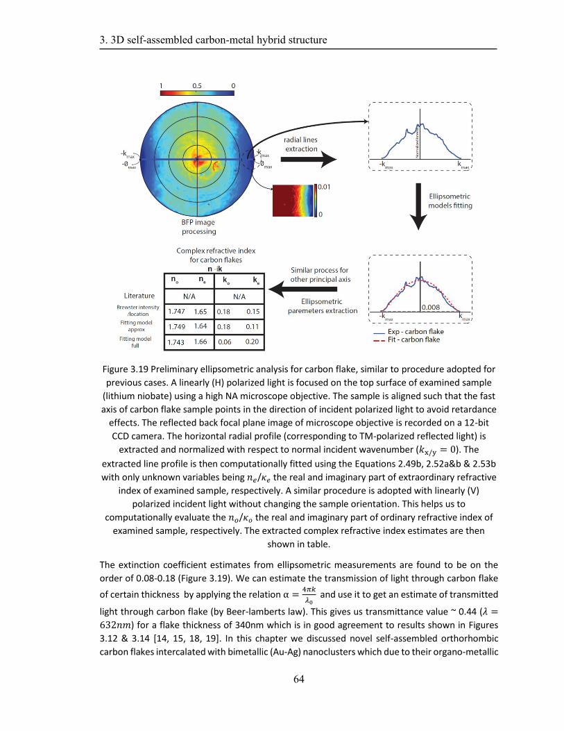
3. 3D self-assembled carbon-metal hybrid structure
64
Figure 3.19 Preliminary ellipsometric analysis for carbon flake, similar to procedure adopted for
previous cases. A linearly (H) polarized light is focused on the top surface of examined sample
(lithium niobate) using a high NA microscope objective. The sample is aligned such that the fast
axis of carbon flake sample points in the direction of incident polarized light to avoid retardance
effects. The reflected back focal plane image of microscope objective is recorded on a 12-bit
CCD camera. The horizontal radial profile (corresponding to TM-polarized reflected light) is
extracted and normalized with respect to normal incident wavenumber (𝑘x/y = 0). The
extracted line profile is then computationally fitted using the Equations 2.49b, 2.52a&b & 2.53b
with only unknown variables being 𝑛𝑒/𝜅𝑒 the real and imaginary part of extraordinary refractive
index of examined sample, respectively. A similar procedure is adopted with linearly (V)
polarized incident light without changing the sample orientation. This helps us to
computationally evaluate the 𝑛𝑜/𝜅𝑜 the real and imaginary part of ordinary refractive index of
examined sample, respectively. The extracted complex refractive index estimates are then
shown in table.
The extinction coefficient estimates from ellipsometric measurements are found to be on the
order of 0.08-0.18 (Figure 3.19). We can estimate the transmission of light through carbon flake
of certain thickness by applying the relation α =4𝜋𝑘
𝜆0 and use it to get an estimate of transmitted
light through carbon flake (by Beer-lamberts law). This gives us transmittance value ~ 0.44 (𝜆 =
632𝑛𝑚) for a flake thickness of 340nm which is in good agreement to results shown in Figures
3.12 & 3.14 [14, 15, 18, 19]. In this chapter we discussed novel self-assembled orthorhombic
carbon flakes intercalated with bimetallic (Au-Ag) nanoclusters which due to their organo-metallic

3. 3D self-assembled carbon-metal hybrid structure
65
nature can find variety of applications in sensing and plasmonic applications [24-26]. we
experimentally investigated the intriguing optical properties in varying fabrication parameters.
With the help of experimental results and theoretical modelling, we relate the high optical
birefringence in the carbon flakes to the crystalline arrangement of carbon atoms in the
orthorhombic lattice [14, 15, 18-20]. We also have made the preliminary estimates of complex
refractive index of the carbon flakes using high NA objective MAI ellipsometry. Due to the high
sensitivity of carbon flakes, they are prone to optical modification which can be utilized for guiding
of light and other opto-electronics applications. The carbon flake, due to its hybrid nature and the
unique phenomenon of self-assembly, still poses many unanswered questions which can only be
answered by continued research. We will discuss some of future projects and research ideas in
Chapter 5 of this thesis.

4. Chiral 2D metasurfaces
In the previous chapter, we discussed a novel self-assembled hybrid structure consisting of an
orthorhombic phase of carbon intercalated with gold-silver nanoclusters. Just like self-assembled
structures, metamaterials/metasurfaces are constructed on the concept of structuring individual
building blocks [7, 32, 35, 42]. We achieve metamaterials by fabricating sub-wavelength scattering
structures called meta-atoms and periodically arranging them. By finely selecting the shape,
orientation, material, and size of meta-atoms, we can tune their optical response [43, 44]. The
field of metamaterials design and analysis has grown extensively since early 2000 due to
technological developments and with lithographic abilities to control surface structuring down to
nanometer scales. Although the concept of negative refractive index and non-unity permeability
was shown by V. G. Veselago [193], but it was the seminal works from J. Pendry, D. Smith and R.
Shelby who experimentally validated and fabricated such metamaterials [194]. Since then,
metamaterials–due to their light controlling and guiding phenomenon, have been used to control
the wave front, intensity, phase, and polarization state of light, both spatially and temporally, and
has instigated interest in many fields of science and industry [38, 43, 44]. Usually, this control over
fine-tuned optical response is achieved by the coupling of incident light waves to electric and
magnetic resonances of the individual meta-atom transpiring overall into control of light
propagation. In the next section, we will first briefly discuss the phenomenon of a chiral optical
response and then later relate it to the design features at the single meta-atom level.
4.1 Chirality and light matter interaction
In Chapter 2, we briefly mentioned the chiral response in the context of circularly polarized light
(in section 2.1.2) and later again while explaining optical activity in a medium (in section 2.3.1)
[63, 96, 195]. The simplest example of this intriguing phenomenon is our hands. Our left and right
hands cannot be superimposed onto each other by simple rotations in 3D-space or, in other
words, they lack mirror-symmetry. A chiral structure and its mirror image are called enantiomers
(also referred to as left and right-handed structures). Hence, a structure which can be
superimposed with its mirror image is called chiral. The most popular quote about the definition
of chirality has been coined by Lord Kelvin [196], who described it in the following way:
“I call any geometrical Figure, or group of points, chiral, and say that it has chirality if its image in
a plane mirror, ideally realized, cannot be brought to coincide with itself.”
The existence of chirality can be abundantly found in nature, ranging from microscopic to
macroscopic scales [197, 198]. Intriguing as it is, the notion of chiral behavior of natural objects,
such as proteins consisting of amino-acids being mainly left-handed and right handedness of
RNA/DNA has baffled researchers for decades [197-199]. As discussed in section 2.3.1, the
polarized light interaction with media/structures having chiral response results in optical activity.
This happens either in the form of circular extinction or circular retardance of light propagation
through such medium [63]. This has also instigated researchers to produce unique designs to
exploit optical activity for scientific and industrial applications [193, 200-205]. However, since its
first report in natural materials, optical activity is usually found to be weak [206]. Hence
4. Chiral 2D metasurfaces
67
considerable effort has been made to produce artificial chiral materials [41, 207-212]. Expanding
on our previous discussion above and in section 2.1.1 & 2.3.1 regarding Maxwell’s equations and
optically active materials, in this section we will try to understand the fundamental idea that
relates them in case of light-matter interaction. For an isotropic homogenous medium, the
respective constitutive relations were discussed earlier. One main consideration of an isotropic
medium is that an electric field (E) and electric displacement (D) are parallel to each other. This
condition holds true also for magnetization [7, 64]. In general, we can assume no magneto-electric
coupling in such media due to orthogonal electric and magnetic fields. In a bi-isotropic medium,
this condition does not remain true anymore and magneto-electric coupling can be observed.
Hence, quantities in the constitutive equations can be generalized mathematically as [213-218],
𝐃 = ε𝐄 +(χ−iγ)
c𝐇, (4.1a)
𝐁 = μ𝐇 +(χ+iγ)
c𝐄, (4.1b)
where 𝜒 & 𝛾 are nonreciprocity and chirality parameters of a medium. The presence of the factor
±𝑖 (phase factor of π/2) in front of the chiral parameter leads 𝑬 & 𝑫 being out of phase [219-221].
For an isotropic medium both 𝜒&𝛾 vanish, while for non-zero values for both factors, they define
a general bi-isotropic medium. For 𝜒 = 0 & 𝛾 ≠ 0, we define a chiral (optically active) medium,
which can be compared to the definition given by Pasteur about inner chirality of a crystal [222].
For 𝜒 ≠ 0 & 𝛾 = 0, represents a nonreciprocal magnetically active medium which produces
asymmetric optical effects in forward and backward propagation directions (also known as
Faraday’s effect) [223].
Building on the constitutive relations for chiral effects, we can derive the chiral wave equation.
The eigen-polarizations of the chiral wave equation are waves with spin angular momentum of
±1 (right and left-handed polarization). For such a wave equation, we relate corresponding wave
vectors for circularly polarized light (𝑘𝑟𝑐𝑝 𝑙𝑐𝑝⁄ ) to refractive indices as (𝑛𝑟𝑐𝑝 𝑙𝑐𝑝⁄ ) [213, 215, 216],
𝑘rcp lcp⁄ =ω
cnrcp lcp⁄ , (4.2a)
𝑛rcp lcp⁄ = n ± γ, (4.2b)
where �� = √휀𝜇 is the nominal refractive index. For a complex value 𝛾, we can relate the real part
of 𝛾 to circular birefringence and imaginary part of 𝛾 to differential circular absorption or circular
dichroism in the context of optical properties. Circularly polarized light is itself chiral, as it hold an
intrinsic sense of handedness (right-handed or left-handed) associated with the rotation of the
electric field vector. Because of this, circularly polarized light is a natural choice for probing chiral
systems. Hence it is intuitive to realize that chiroptical effects arise because of the fact that
incident circularly polarized light experiences different complex refractive indices for two circular
handedness. This can be linked directly to the definition of optical activity, discussed in section
2.3.1 and Appendix A to this thesis. In terms of a Müller matrix of a chiral structure (as shown in
Figure 2.7), optical activity corresponds to the cross-diagonal Müller matrix elements.
4. Chiral 2D metasurfaces
68
Chiral light matter interaction
The main aim in the design of chiral meta-atom is to increase chirality of individual meta-atom or
find other ways to increase the chiroptical effect. These effects can then be coupled to far field
by carefully designing a periodic array of meta-atoms. Similar to constitutive chiral relations, we
can describe chiral meta-atoms based on induced dipole moments which depend on induvial
electric, magnetic and cross polarizations [224]. At individual meta-atom level this relates to
electric and magnetic moments and resonances [225]. In this case, for a single meta-atom the
differential absorption (Δ𝑎) for incident left and right circularly polarized light is defined as [226],
Δ𝑎 =2
0ℑ(𝛼𝑒𝑚)Δ𝐶, (4.3)
where (𝛼𝑒𝑚) is magneto-electric cross-polarizability and Δ𝐶 defines the differential optical
chirality density for right and left circularly polarized light, and for monochromatic light wave the
case simplifies to,
C = − 0𝜔
2ℑ(𝐸∗. 𝐵). (4.4)
Hence the chiral effects can be considered a combination of chirality density of induvial meta-
atom and chiral incident fields. Cohen et. al. produced another mathematically elegant way to
describe the chiral effects mentioned above in terms of dissymmetry factor (g)[67, 227],
𝑔 = −ℑ(𝛼𝑒𝑚
𝛼𝑒) (
2𝐶
𝜔𝑈𝑒), (4.5)
where 𝑈𝑒 is the time average electric energy density. This equation holds true for any parity
interchangeable light waves. For a circularly polarized light they reduce to,
𝑔𝐶𝑃𝐿 = −ℑ(𝛼𝑒𝑚
𝛼𝑒) (
4
𝑐). (4.6)
Many a times, a meta-atom is achiral, but still can produce chiral optical response when probed
with circularly polarized light beams. In this chapter we will concentrate on such structures. Based
on design, composition, and orientation of such meta-atom we can induce specific electric or
magnetic resonances which leads to chiral response [16] (see Figure 4.1).
Concept of 2D and 3D chirality
In the literature, usually two variants of chirality (in terms of dimensionality) are discussed [100,
228]. A 2D meta-atom usually would have sub-wavelength thickness and sometimes are referred
to as metasurfaces (Figure 4.1). For instance, THz metasurfaces, the thickness of meta-atom
would be in the order of 20-100nm. On contrary, 3D meta-atoms have thickness greater than that
and are usually referred to as 3D-metastructures.
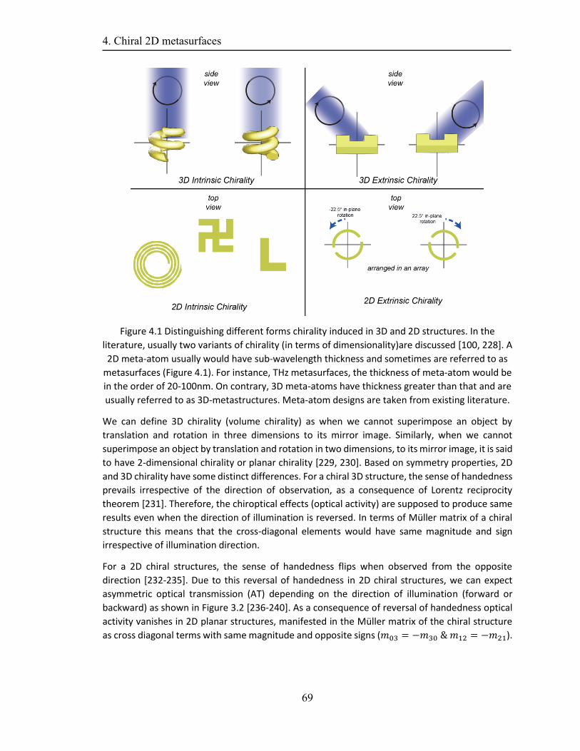
4. Chiral 2D metasurfaces
69
Figure 4.1 Distinguishing different forms chirality induced in 3D and 2D structures. In the
literature, usually two variants of chirality (in terms of dimensionality)are discussed [100, 228]. A
2D meta-atom usually would have sub-wavelength thickness and sometimes are referred to as
metasurfaces (Figure 4.1). For instance, THz metasurfaces, the thickness of meta-atom would be
in the order of 20-100nm. On contrary, 3D meta-atoms have thickness greater than that and are
usually referred to as 3D-metastructures. Meta-atom designs are taken from existing literature.
We can define 3D chirality (volume chirality) as when we cannot superimpose an object by
translation and rotation in three dimensions to its mirror image. Similarly, when we cannot
superimpose an object by translation and rotation in two dimensions, to its mirror image, it is said
to have 2-dimensional chirality or planar chirality [229, 230]. Based on symmetry properties, 2D
and 3D chirality have some distinct differences. For a chiral 3D structure, the sense of handedness
prevails irrespective of the direction of observation, as a consequence of Lorentz reciprocity
theorem [231]. Therefore, the chiroptical effects (optical activity) are supposed to produce same
results even when the direction of illumination is reversed. In terms of Müller matrix of a chiral
structure this means that the cross-diagonal elements would have same magnitude and sign
irrespective of illumination direction.
For a 2D chiral structures, the sense of handedness flips when observed from the opposite
direction [232-235]. Due to this reversal of handedness in 2D chiral structures, we can expect
asymmetric optical transmission (AT) depending on the direction of illumination (forward or
backward) as shown in Figure 3.2 [236-240]. As a consequence of reversal of handedness optical
activity vanishes in 2D planar structures, manifested in the Müller matrix of the chiral structure
as cross diagonal terms with same magnitude and opposite signs (𝑚03 = −𝑚30 & 𝑚12 = −𝑚21).
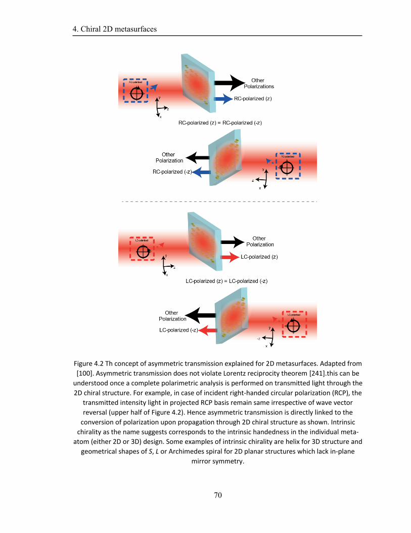
4. Chiral 2D metasurfaces
70
Figure 4.2 Th concept of asymmetric transmission explained for 2D metasurfaces. Adapted from
[100]. Asymmetric transmission does not violate Lorentz reciprocity theorem [241].this can be
understood once a complete polarimetric analysis is performed on transmitted light through the
2D chiral structure. For example, in case of incident right-handed circular polarization (RCP), the
transmitted intensity light in projected RCP basis remain same irrespective of wave vector
reversal (upper half of Figure 4.2). Hence asymmetric transmission is directly linked to the
conversion of polarization upon propagation through 2D chiral structure as shown. Intrinsic
chirality as the name suggests corresponds to the intrinsic handedness in the individual meta-
atom (either 2D or 3D) design. Some examples of intrinsic chirality are helix for 3D structure and
geometrical shapes of S, L or Archimedes spiral for 2D planar structures which lack in-plane
mirror symmetry.
4. Chiral 2D metasurfaces
71
Hence, optical activity can be related to 3D chirality, while 2D chirality is studied in terms of
asymmetric transmission in literature [236-240].
Asymmetric transmission does not violate Lorentz reciprocity theorem as shown in Figure 4.2
[241].this can be understood once a complete polarimetric analysis is performed on transmitted
light through the 2D chiral structure. For example, in case of incident right-handed circular
polarization (RCP), the transmitted intensity light in projected RCP basis remain same irrespective
of wave vector reversal (upper half of Figure 4.2). Hence asymmetric transmission is directly linked
to the conversion of polarization upon propagation through 2D chiral structure as shown in Figure
4.2.
Intrinsic/extrinsic chirality
In Equation 4.6 we discussed that the chiroptical response is a manifestation of either individual
meta-atom response or the polarization nature of impinging light wave. Hence, it is important to
discuss the cases of 2D and 3D chirality [234, 242] in the context of intrinsic and extrinsic chirality.
Intrinsic chirality as the name suggests corresponds to the intrinsic handedness in the individual
meta-atom (either 2d or 3D) design. Some examples of intrinsic chirality are helix for 3D structure
and geometrical shapes of S, L or Archimedes spiral for 2D planar structures which lack in-plane
mirror symmetry [243-247] as shown in Figure 4.1.
In essence, it is possible for an intrinsically achiral structure to produce chiral optical effects. This
is defined in literature as extrinsic or pseudo chirality. It can be manifested in number of ways
including, heterogeneity or arrangements of individual achiral structures, the phase, angular
spectrum, and polarization of incident light wave can be adjusted to lead to a chiroptical response
form the structure [53, 210, 234, 248-257]. Extrinsic chirality has been an intense field of study in
the last decade and has found applications in multiple fields of science [210, 234, 253-255].
In this chapter, we will discuss the special case of a 2D fourfold symmetric achiral meta-atom
(quadrumer) to induce desired asymmetric transmission by extrinsic chirality. We will start with
understanding the in-plane scattering from an achiral individual quadrumer. Later we will discuss
ways to couple the in-plane scattering of an individual quadrumer to far fields by placing them in
a periodic array.
Quadrumer design and surface lattice resonances
The simulations discussed in this section were conceptualized optimized and performed by
Professor (Assistant) Dr. N. Apurv Chaitanya. We consider the case of an achiral (four-fold
symmetric) structure consisting of four rectangular bars arranged in a square configuration, as
shown in Figure 4.3[16]. The lateral dimensions of each bar are 160nm x 80nm, while thickness is
kept to 20nm, hence can be considered as a 2D metastrucutre. We choose gold as material for
quadrumer for which the refractive index model is chosen from standard literature [258]. We use
finite difference time domain method (FDTD) [259] to simulate the said structure by
computationally solving fully vectorial Maxwell equations for light propagation and interaction.
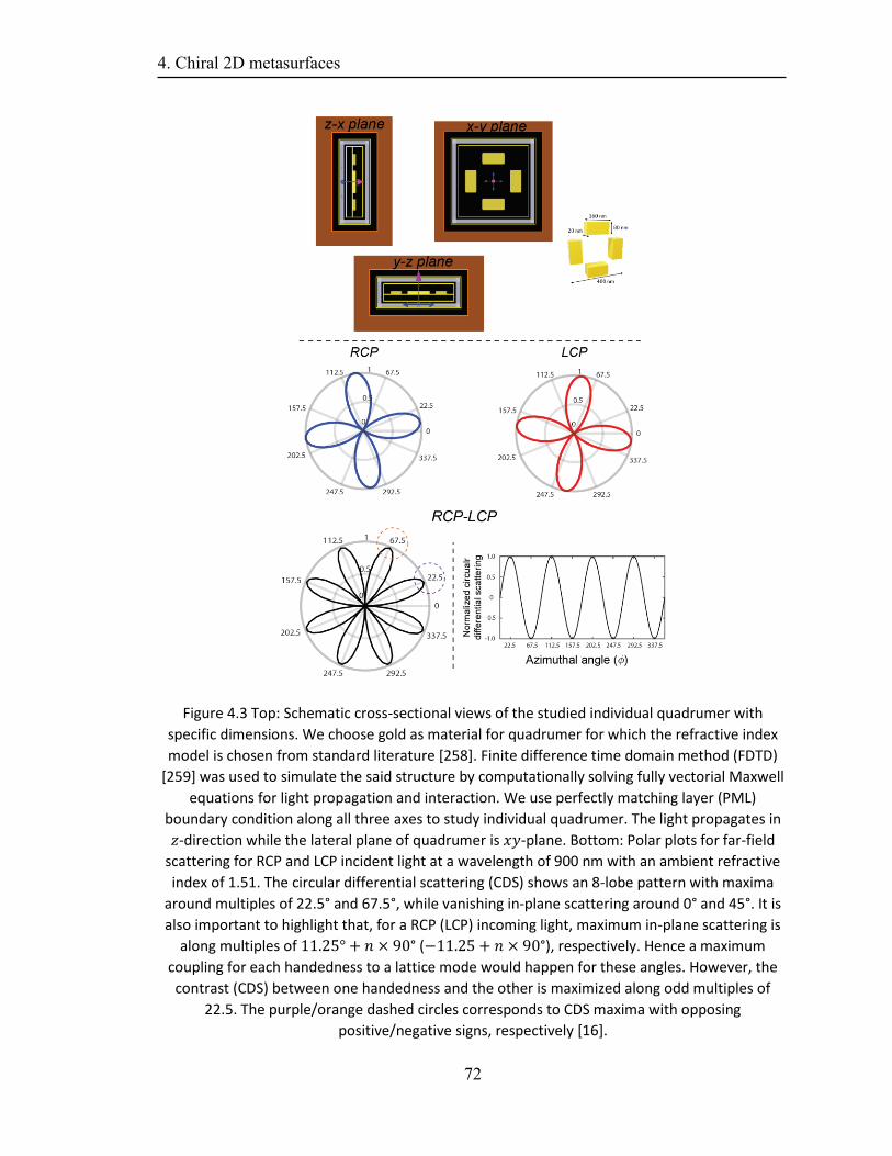
4. Chiral 2D metasurfaces
72
Figure 4.3 Top: Schematic cross-sectional views of the studied individual quadrumer with
specific dimensions. We choose gold as material for quadrumer for which the refractive index
model is chosen from standard literature [258]. Finite difference time domain method (FDTD)
[259] was used to simulate the said structure by computationally solving fully vectorial Maxwell
equations for light propagation and interaction. We use perfectly matching layer (PML)
boundary condition along all three axes to study individual quadrumer. The light propagates in
𝑧-direction while the lateral plane of quadrumer is 𝑥𝑦-plane. Bottom: Polar plots for far-field
scattering for RCP and LCP incident light at a wavelength of 900 nm with an ambient refractive
index of 1.51. The circular differential scattering (CDS) shows an 8-lobe pattern with maxima
around multiples of 22.5° and 67.5°, while vanishing in-plane scattering around 0° and 45°. It is
also important to highlight that, for a RCP (LCP) incoming light, maximum in-plane scattering is
along multiples of 11.25° + 𝑛 × 90° (−11.25 + 𝑛 × 90°), respectively. Hence a maximum
coupling for each handedness to a lattice mode would happen for these angles. However, the
contrast (CDS) between one handedness and the other is maximized along odd multiples of
22.5. The purple/orange dashed circles corresponds to CDS maxima with opposing
positive/negative signs, respectively [16].
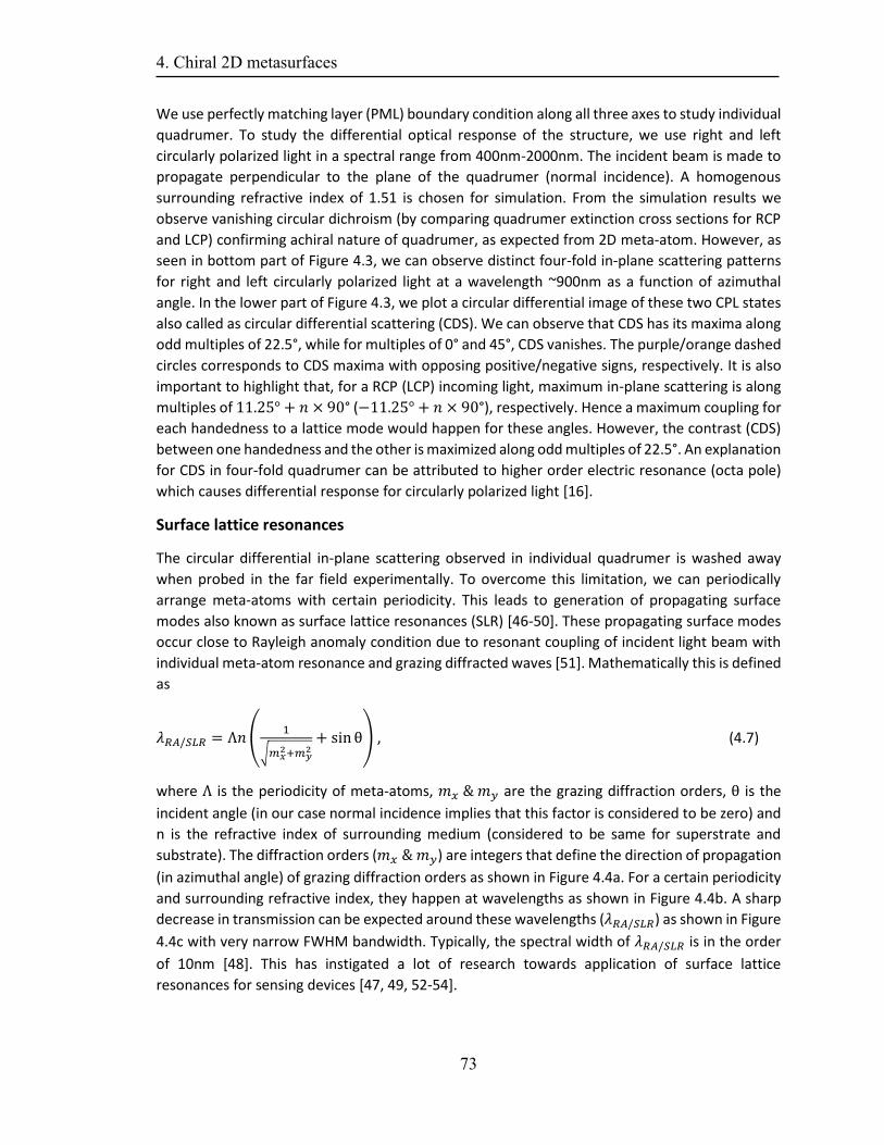
4. Chiral 2D metasurfaces
73
We use perfectly matching layer (PML) boundary condition along all three axes to study individual
quadrumer. To study the differential optical response of the structure, we use right and left
circularly polarized light in a spectral range from 400nm-2000nm. The incident beam is made to
propagate perpendicular to the plane of the quadrumer (normal incidence). A homogenous
surrounding refractive index of 1.51 is chosen for simulation. From the simulation results we
observe vanishing circular dichroism (by comparing quadrumer extinction cross sections for RCP
and LCP) confirming achiral nature of quadrumer, as expected from 2D meta-atom. However, as
seen in bottom part of Figure 4.3, we can observe distinct four-fold in-plane scattering patterns
for right and left circularly polarized light at a wavelength ~900nm as a function of azimuthal
angle. In the lower part of Figure 4.3, we plot a circular differential image of these two CPL states
also called as circular differential scattering (CDS). We can observe that CDS has its maxima along
odd multiples of 22.5°, while for multiples of 0° and 45°, CDS vanishes. The purple/orange dashed
circles corresponds to CDS maxima with opposing positive/negative signs, respectively. It is also
important to highlight that, for a RCP (LCP) incoming light, maximum in-plane scattering is along
multiples of 11.25° + 𝑛 × 90° (−11.25° + 𝑛 × 90°), respectively. Hence a maximum coupling for
each handedness to a lattice mode would happen for these angles. However, the contrast (CDS)
between one handedness and the other is maximized along odd multiples of 22.5°. An explanation
for CDS in four-fold quadrumer can be attributed to higher order electric resonance (octa pole)
which causes differential response for circularly polarized light [16].
Surface lattice resonances
The circular differential in-plane scattering observed in individual quadrumer is washed away
when probed in the far field experimentally. To overcome this limitation, we can periodically
arrange meta-atoms with certain periodicity. This leads to generation of propagating surface
modes also known as surface lattice resonances (SLR) [46-50]. These propagating surface modes
occur close to Rayleigh anomaly condition due to resonant coupling of incident light beam with
individual meta-atom resonance and grazing diffracted waves [51]. Mathematically this is defined
as
𝜆𝑅𝐴/𝑆𝐿𝑅 = Λ𝑛 (1
√𝑚𝑥2+𝑚𝑦
2+ sinθ) , (4.7)
where Λ is the periodicity of meta-atoms, 𝑚𝑥 & 𝑚𝑦 are the grazing diffraction orders, θ is the
incident angle (in our case normal incidence implies that this factor is considered to be zero) and
n is the refractive index of surrounding medium (considered to be same for superstrate and
substrate). The diffraction orders (𝑚𝑥 & 𝑚𝑦) are integers that define the direction of propagation
(in azimuthal angle) of grazing diffraction orders as shown in Figure 4.4a. For a certain periodicity
and surrounding refractive index, they happen at wavelengths as shown in Figure 4.4b. A sharp
decrease in transmission can be expected around these wavelengths (𝜆𝑅𝐴/𝑆𝐿𝑅) as shown in Figure
4.4c with very narrow FWHM bandwidth. Typically, the spectral width of 𝜆𝑅𝐴/𝑆𝐿𝑅 is in the order
of 10nm [48]. This has instigated a lot of research towards application of surface lattice
resonances for sensing devices [47, 49, 52-54].
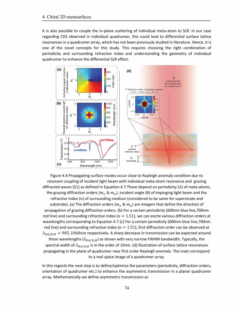
4. Chiral 2D metasurfaces
74
It is also possible to couple the in-plane scattering of individual meta-atom to SLR. In our case
regarding CDS observed in individual quadrumer, this could lead to differential surface lattice
resonances in a quadrumer array, which has not been previously studied in literature. Hence, it is
one of the novel concepts for this study. This requires choosing the right combination of
periodicity and surrounding refractive index and understanding the geometry of individual
quadrumer to enhance the differential SLR effect.
Figure 4.4 Propagating surface modes occur close to Rayleigh anomaly condition due to
resonant coupling of incident light beam with individual meta-atom resonance and grazing
diffracted waves [51] as defined in Equation 4.7.These depend on periodicity (Λ) of meta-atoms,
the grazing diffraction orders (𝑚𝑥 & 𝑚𝑦), incident angle (θ) of impinging light beam and the
refractive index (𝑛) of surrounding medium (considered to be same for superstrate and
substrate). (a) The diffraction orders (𝑚𝑥 & 𝑚𝑦) are integers that define the direction of
propagation of grazing diffraction orders. (b) For a certain periodicity (600nm blue line,700nm
red line) and surrounding refractive index (n = 1.51), we can excite various diffraction orders at
wavelengths corresponding to Equation 4.7.(c) For a certain periodicity (600nm blue line,700nm
red line) and surrounding refractive index (n = 1.51), first diffraction order can be observed at
𝜆𝑅𝐴/𝑆𝐿𝑅 = 905, 1060𝑛𝑚 respectively. A sharp decrease in transmission can be expected around
these wavelengths (𝜆𝑅𝐴/𝑆𝐿𝑅) as shown with very narrow FWHM bandwidth. Typically, the
spectral width of 𝜆𝑅𝐴/𝑆𝐿𝑅 is in the order of 10nm. (d) Illustration of surface lattice resonances
propagating in the plane of quadrumer near first order Rayleigh anomaly. The inset correspond
to a real space image of a quadrumer array.
In this regards the next step is to define/optimize the parameters (periodicity, diffraction orders,
orientation of quadrumer etc.) to enhance the asymmetric transmission in a planar quadrumer
array. Mathematically we define asymmetric transmission as
4. Chiral 2D metasurfaces
75
AT =(𝐼𝑅𝐶𝑃−𝐼𝐿𝐶𝑃)
𝐼𝑅𝐶𝑃+𝐼𝐿𝐶𝑃. (4.8)
Where 𝐼𝑅𝐶𝑃 , 𝐼𝐿𝐶𝑃 are the transmitted intensity for case of RCP,LCP polarized incident light. We can
decompose the total transmitted intensity (for respective) into intensities correspond to certain
diffraction orders. As evident from discussion above, the differential SLR should lead to higher AT
near Rayleigh anomaly for higher diffraction orders (neglecting zeroth diffraction order). As we
move away from the Rayleigh anomaly condition the differential coupling to SLRs decreases
resulting in reduced AT. The extreme case is when the diffracted beam becomes normal to the
planar quadrumer array, where the diffracted beam has same transmitted power for RCP and LCP
incident light beam. Hence, Due to symmetry reasons no AT is observed in zeroth diffraction
order. To understand and optimize the phenomenon of asymmetric transmission in planar
quadrumer array, we perform a FDTD simulation of a quadrumer with periodic boundary
conditions in the lateral plane of quadrumer and PML boundary condition along the direction of
light propagation [16]. We choose to study asymmetric transmission in the first diffraction orders
as shown in Figure 4.4d (for illustrative purposes). The insets correspond to a real space image of
recorded surface lattice mode). An in-plane rotation of individual quadrumer leads to an
equivalent rotation of the in-plane scattering. This rotation can lead to efficient coupling of in-
plane scattering to surface lattice resonances of first diffraction order, resulting in enhanced AT.
Figure 4.5 SEM micrograph of fabricated quadrumer array. The nanofabrication was done on N-
BK7 cover glass with thickness of 170 microns without any adhesion layer (fabrication done by
and pictures courtesy of Dr. Orad Reshef, University of Ottawa, Canada).
The simulations were performed for varying orientations (in plane rotation of quadrumer ranging
from -45°to 45°). We chose four orientations which are of importance, i.e. 0°,22.5°,45°and –
22.5°(corresponds to 67.5°). These orientations were chosen based on the maxima/minima of
CDS observed in single quadrumer simulation. A sweep of periodicity was performed from 500-
1000nm. The simulation results pointed towards enhanced AT for the case of 600nm periodicity
of quadrumer. Hence the sample was fabricated with said periodicity and orientations.
200 m
1 m
22.5
22.5
45
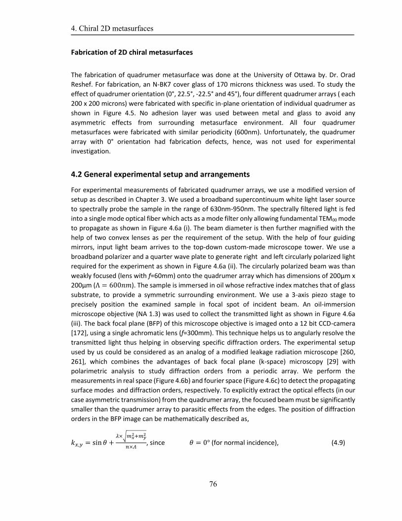
4. Chiral 2D metasurfaces
76
Fabrication of 2D chiral metasurfaces
The fabrication of quadrumer metasurface was done at the University of Ottawa by. Dr. Orad
Reshef. For fabrication, an N-BK7 cover glass of 170 microns thickness was used. To study the
effect of quadrumer orientation (0°, 22.5°, -22.5° and 45°), four different quadrumer arrays ( each
200 x 200 microns) were fabricated with specific in-plane orientation of individual quadrumer as
shown in Figure 4.5. No adhesion layer was used between metal and glass to avoid any
asymmetric effects from surrounding metasurface environment. All four quadrumer
metasurfaces were fabricated with similar periodicity (600nm). Unfortunately, the quadrumer
array with 0° orientation had fabrication defects, hence, was not used for experimental
investigation.
4.2 General experimental setup and arrangements
For experimental measurements of fabricated quadrumer arrays, we use a modified version of
setup as described in Chapter 3. We used a broadband supercontinuum white light laser source
to spectrally probe the sample in the range of 630nm-950nm. The spectrally filtered light is fed
into a single mode optical fiber which acts as a mode filter only allowing fundamental TEM00 mode
to propagate as shown in Figure 4.6a (i). The beam diameter is then further magnified with the
help of two convex lenses as per the requirement of the setup. With the help of four guiding
mirrors, input light beam arrives to the top-down custom-made microscope tower. We use a
broadband polarizer and a quarter wave plate to generate right and left circularly polarized light
required for the experiment as shown in Figure 4.6a (ii). The circularly polarized beam was than
weakly focused (lens with f=60mm) onto the quadrumer array which has dimensions of 200µm x
200µm (Λ = 600𝑛𝑚). The sample is immersed in oil whose refractive index matches that of glass
substrate, to provide a symmetric surrounding environment. We use a 3-axis piezo stage to
precisely position the examined sample in focal spot of incident beam. An oil-immersion
microscope objective (NA 1.3) was used to collect the transmitted light as shown in Figure 4.6a
(iii). The back focal plane (BFP) of this microscope objective is imaged onto a 12 bit CCD-camera
[172], using a single achromatic lens (f=300mm). This technique helps us to angularly resolve the
transmitted light thus helping in observing specific diffraction orders. The experimental setup
used by us could be considered as an analog of a modified leakage radiation microscope [260,
261], which combines the advantages of back focal plane (k-space) microscopy [29] with
polarimetric analysis to study diffraction orders from a periodic array. We perform the
measurements in real space (Figure 4.6b) and fourier space (Figure 4.6c) to detect the propagating
surface modes and diffraction orders, respectively. To explicitly extract the optical effects (in our
case asymmetric transmission) from the quadrumer array, the focused beam must be significantly
smaller than the quadrumer array to parasitic effects from the edges. The position of diffraction
orders in the BFP image can be mathematically described as,
𝑘𝑥,𝑦 = sin 𝜃 +𝜆×√𝑚𝑥
2+𝑚𝑦2
𝑛×𝛬, since 𝜃 = 0° (for normal incidence), (4.9)
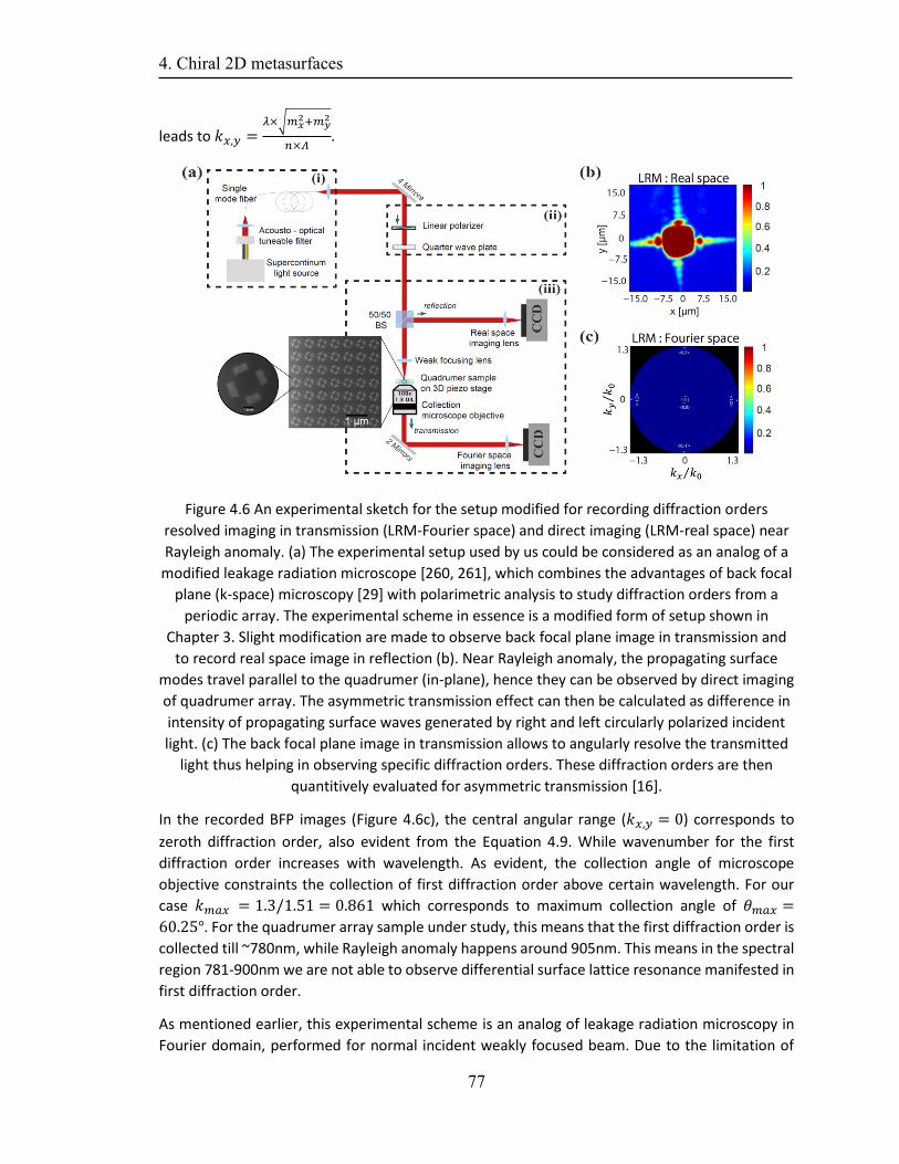
4. Chiral 2D metasurfaces
77
leads to 𝑘𝑥,𝑦 =𝜆×√𝑚𝑥
2+𝑚𝑦2
𝑛×𝛬.
Figure 4.6 An experimental sketch for the setup modified for recording diffraction orders
resolved imaging in transmission (LRM-Fourier space) and direct imaging (LRM-real space) near
Rayleigh anomaly. (a) The experimental setup used by us could be considered as an analog of a
modified leakage radiation microscope [260, 261], which combines the advantages of back focal
plane (k-space) microscopy [29] with polarimetric analysis to study diffraction orders from a
periodic array. The experimental scheme in essence is a modified form of setup shown in
Chapter 3. Slight modification are made to observe back focal plane image in transmission and
to record real space image in reflection (b). Near Rayleigh anomaly, the propagating surface
modes travel parallel to the quadrumer (in-plane), hence they can be observed by direct imaging
of quadrumer array. The asymmetric transmission effect can then be calculated as difference in
intensity of propagating surface waves generated by right and left circularly polarized incident
light. (c) The back focal plane image in transmission allows to angularly resolve the transmitted
light thus helping in observing specific diffraction orders. These diffraction orders are then
quantitively evaluated for asymmetric transmission [16].
In the recorded BFP images (Figure 4.6c), the central angular range (𝑘𝑥,𝑦 = 0) corresponds to
zeroth diffraction order, also evident from the Equation 4.9. While wavenumber for the first
diffraction order increases with wavelength. As evident, the collection angle of microscope
objective constraints the collection of first diffraction order above certain wavelength. For our
case 𝑘𝑚𝑎𝑥 = 1.3/1.51 = 0.861 which corresponds to maximum collection angle of 𝜃𝑚𝑎𝑥 =
60.25°. For the quadrumer array sample under study, this means that the first diffraction order is
collected till ~780nm, while Rayleigh anomaly happens around 905nm. This means in the spectral
region 781-900nm we are not able to observe differential surface lattice resonance manifested in
first diffraction order.
As mentioned earlier, this experimental scheme is an analog of leakage radiation microscopy in
Fourier domain, performed for normal incident weakly focused beam. Due to the limitation of
4. Chiral 2D metasurfaces
78
collection microscope objective, the asymmetric transmission effects in first diffraction order near
Rayleigh anomaly cannot be observed. Thus, while our technique to observe diffraction order
based asymmetric transmission has a certain drawback, it is still preferable for observing optical
properties at only normal incidence condition. This way, we can avoid patristic extrinsic chirality
emerging from the angular spectrum, when using focused light-based experimental setups. This
method also helps in observing the coupling of incident light beam to various diffraction orders
at normal incidence, which can be useful in the future to study higher orders differential surface
lattice resonances in rotationally symmetric achiral structures.
To observe qualitatively the asymmetric transmission at Rayleigh anomaly, we performed leakage
radiation microscopy in real space in reflection. Near Rayleigh anomaly as explained above, the
propagating surface modes travel parallel to the quadrumer (in-plane), hence they can be
observed by direct imaging of quadrumer array. This was done by placing an imaging lens in the
reflection arm and recording the real space image on a CCD camera. As shown in Figure 4.6b. The
asymmetric transmission effect can then be calculated as pixel-by-pixel difference in intensity
images of propagating surface waves generated by right and left circularly polarized light.
4.3 Results and discussion (asymmetric transmission of quadrumer array)
We experimentally evaluated the three cases of 45°, 22.5° and -22.5° in-plane rotation of the
meta-atom to understand the asymmetric transmission in zeroth and first diffraction orders. In
the following we discuss some salient aspects of the results and discuss them in light of
simulations. We will also elaborate on certain interesting outcomes, which can be interesting for
future projects.
Observing Rayleigh anomaly
As discussed in section 4.1.3, the presence of propagating surface modes near Rayleigh anomaly
results in sharp drop in total transmission, which is dependent on periodicity of meta-atoms and
their surrounding refractive index. It is pertinent to highlight that this effect is independent of
material composition of individual meta-atom. In top part of Figure 4.7, photo diode (PD) based
scan image of the transmitted optical intensity when scanning the quadrumer array through the
focal field distribution can be found. The sharp edges of the array confirms the confocal
arrangement of the focusing lens and collection objective with quadrumer array present in the
focal plane of focusing objective. Hence, the PD based measurement was used to precisely align
the examined quadrumer array in the focal spot. These measurements helped us in confirming
the presence of propagating surface modes near Rayleigh anomaly due to sudden drop in
transmission. This can be observed in bottom part of Figure 4.7. where both simulation and
experimental results are plotted. In the course of this thesis, we tried different combinations of
focusing lens as shown in bottom part of Figure 4.7. Some results for high NA focusing objective
(NA 0.9) are shown in Appendix C to this thesis. As expected, the use of higher NA focusing lens,
spectrally broadens the transmission drop near Rayleigh anomaly and can lead to patristic
extrinsic chirality emerging from the angular spectrum of focusing lens.
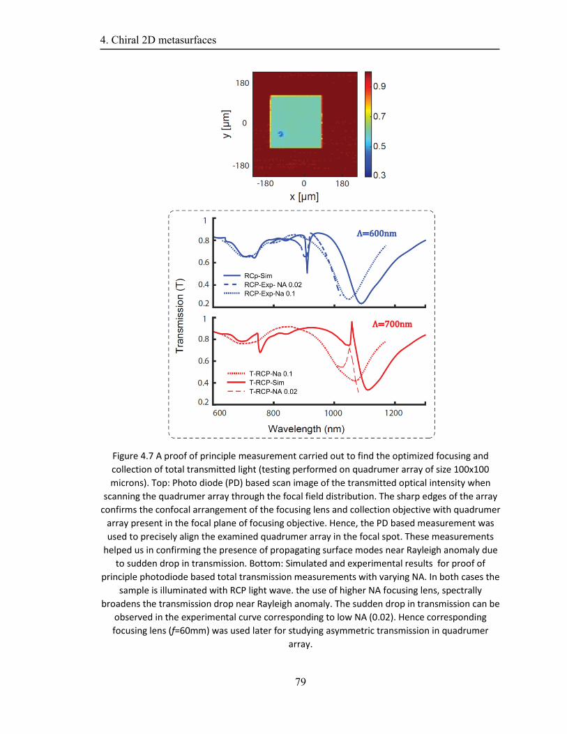
4. Chiral 2D metasurfaces
79
Figure 4.7 A proof of principle measurement carried out to find the optimized focusing and
collection of total transmitted light (testing performed on quadrumer array of size 100x100
microns). Top: Photo diode (PD) based scan image of the transmitted optical intensity when
scanning the quadrumer array through the focal field distribution. The sharp edges of the array
confirms the confocal arrangement of the focusing lens and collection objective with quadrumer
array present in the focal plane of focusing objective. Hence, the PD based measurement was
used to precisely align the examined quadrumer array in the focal spot. These measurements
helped us in confirming the presence of propagating surface modes near Rayleigh anomaly due
to sudden drop in transmission. Bottom: Simulated and experimental results for proof of
principle photodiode based total transmission measurements with varying NA. In both cases the
sample is illuminated with RCP light wave. the use of higher NA focusing lens, spectrally
broadens the transmission drop near Rayleigh anomaly. The sudden drop in transmission can be
observed in the experimental curve corresponding to low NA (0.02). Hence corresponding
focusing lens (f=60mm) was used later for studying asymmetric transmission in quadrumer
array.
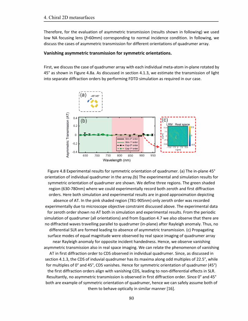
4. Chiral 2D metasurfaces
80
Therefore, for the evaluation of asymmetric transmission (results shown in following) we used
low NA focusing lens (f=60mm) corresponding to normal incidence condition. In following, we
discuss the cases of asymmetric transmission for different orientations of quadrumer array.
Vanishing asymmetric transmission for symmetric orientations.
First, we discuss the case of quadrumer array with each individual meta-atom in-plane rotated by
45° as shown in Figure 4.8a. As discussed in section 4.1.3, we estimate the transmission of light
into separate diffraction orders by performing FDTD simulation as required in our case.
Figure 4.8 Experimental results for symmetric orientation of quadrumer. (a) The in-plane 45°
orientation of individual quadrumer in the array.(b) The experimental and simulation results for
symmetric orientation of quadrumer are shown. We define three regions. The green shaded
region (630-780nm) where we could experimentally record both zeroth and first diffraction
orders. Here both simulation and experimental results are in good approximation depicting
absence of AT. In the pink shaded region (781-905nm) only zeroth order was recorded
experimentally due to microscope objective constraint discussed above. The experimental data
for zeroth order shown no AT both in simulation and experimental results. From the periodic
simulation of quadrumer (all orientations) and from Equation 4.7 we also observe that there are
no diffracted waves travelling parallel to quadrumer (in-plane) after Rayleigh anomaly. Thus, no
differential SLR are formed leading to absence of asymmetric transmission. (c) Propagating
surface modes of equal magnitude were observed by real space imaging of quadrumer array
near Rayleigh anomaly for opposite incident handedness. Hence, we observe vanishing
asymmetric transmission also in real space imaging. We can relate the phenomenon of vanishing
AT in first diffraction order to CDS observed in individual quadrumer. Since, as discussed in
section 4.1.3, the CDS of induvial quadrumer has its maxima along odd multiples of 22.5°, while
for multiples of 0° and 45°, CDS vanishes. Hence for symmetric orientation of quadrumer (45°)
the first diffraction orders align with vanishing CDS, leading to non-differential effects in SLR.
Resultantly, no asymmetric transmission is observed in first diffraction order. Since 0° and 45°
both are example of symmetric orientation of quadrumer, hence we can safely assume both of
them to behave optically in similar manner [16].
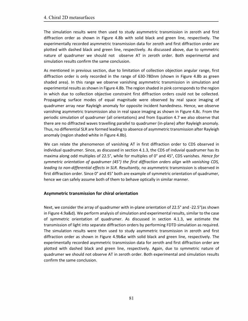
4. Chiral 2D metasurfaces
81
The simulation results were then used to study asymmetric transmission in zeroth and first
diffraction order as shown in Figure 4.8b with solid black and green line, respectively. The
experimentally recorded asymmetric transmission data for zeroth and first diffraction order are
plotted with dashed black and green line, respectively. As discussed above, due to symmetric
nature of quadrumer we should not observe AT in zeroth order. Both experimental and
simulation results confirm the same conclusion.
As mentioned in previous section, due to limitation of collection objection angular range, first
diffraction order is only recorded in the range of 630-780nm (shown in Figure 4.8b as green
shaded area). In this range we observe vanishing asymmetric transmission in simulation and
experimental results as shown in Figure 4.8b. The region shaded in pink corresponds to the region
in which due to collection objective constraint first diffraction orders could not be collected.
Propagating surface modes of equal magnitude were observed by real space imaging of
quadrumer array near Rayleigh anomaly for opposite incident handedness. Hence, we observe
vanishing asymmetric transmission also in real space imaging as shown in Figure 4.8c. From the
periodic simulation of quadrumer (all orientations) and from Equation 4.7 we also observe that
there are no diffracted waves travelling parallel to quadrumer (in-plane) after Rayleigh anomaly.
Thus, no differential SLR are formed leading to absence of asymmetric transmission after Rayleigh
anomaly (region shaded white in Figure 4.8b).
We can relate the phenomenon of vanishing AT in first diffraction order to CDS observed in
individual quadrumer. Since, as discussed in section 4.1.3, the CDS of induvial quadrumer has its
maxima along odd multiples of 22.5°, while for multiples of 0° and 45°, CDS vanishes. Hence for
symmetric orientation of quadrumer (45°) the first diffraction orders align with vanishing CDS,
leading to non-differential effects in SLR. Resultantly, no asymmetric transmission is observed in
first diffraction order. Since 0° and 45° both are example of symmetric orientation of quadrumer,
hence we can safely assume both of them to behave optically in similar manner.
Asymmetric transmission for chiral orientation
Next, we consider the array of quadrumer with in-plane orientation of 22.5° and -22.5°(as shown
in Figure 4.9a&d). We perform analysis of simulation and experimental results, similar to the case
of symmetric orientation of quadrumer. As discussed in section 4.1.3, we estimate the
transmission of light into separate diffraction orders by performing FDTD simulation as required.
The simulation results were then used to study asymmetric transmission in zeroth and first
diffraction order as shown in Figure 4.9b&e with solid black and green line, respectively. The
experimentally recorded asymmetric transmission data for zeroth and first diffraction order are
plotted with dashed black and green line, respectively. Again, due to symmetric nature of
quadrumer we should not observe AT in zeroth order. Both experimental and simulation results
confirm the same conclusion.
4. Chiral 2D metasurfaces
82
Figure 4.9 Experimental results for symmetric orientation of quadrumer (a,d). The in-plane 22.5°
& -22.5° orientation of individual quadrumer in the array. (b,e) The experimental and simulation
results for chiral orientation of quadrumer are shown. We define three regions. The green
shaded region (630-780nm) where we could experimentally record both zeroth and first
diffraction orders. Here both simulation and experimental results are in good approximation
depicting presence of AT in first diffraction order. In the pink shaded region (781-905nm) only
zeroth order was recorded experimentally due to microscope objective constraint discussed
above. The experimental data for zeroth order shown no AT both in simulation and
experimental results. From the periodic simulation of quadrumer (all orientations) and from
Equation 4.7 we also observe that there are no diffracted waves travelling parallel to quadrumer
(in-plane) after Rayleigh anomaly. Thus, no differential SLR are formed leading to absence of AT.
This was also experimentally confirmed (in the region shaded white, from 906-960nm). (c&e)
are differential images evaluating AT in similar fashion as described above for diffraction orders.
For the chiral orientation (22.5° and -22.5° orientation), we observe asymmetric propagating
modes with opposite signs as expected also from simulation results [16].
4. Chiral 2D metasurfaces
83
The simulation results clearly show the presence of high AT, closer to wavelengths supporting
Rayleigh anomaly condition and therefore depicting the significance of SLRs in observing AT in 2D
metasurfaces. Towards shorter wavelengths, the value of AT decreases. For the case of symmetric
orientation (0°and 45°) discussed above we saw vanishing AT in first diffraction order. For the
present case of in-plane rotation of 22.5 and -22.5°, we observe AT in first diffraction order as
shown in Figure 4.9b&e. The simulation and experimental results for AT show good agreement in
the region shaded green where the first diffraction order was recorded. We observe AT with
opposite signs and equal magnitude for the case of 22.5 and -22,5°in plane orientation of
quadrumer. As mentioned, above the first diffraction order was not collected in the region shaded
pink. For propagating surface modes near Rayleigh anomaly, we perform real space measurement
for opposite incident light beam handedness to estimate AT. The images (Figure 4.9c&d) are
differential images evaluating AT in similar fashion as described above for diffraction orders. We
observe asymmetric propagating modes with opposite signs (Figure 4.9c&d) similar to
quantitative results shown in Figure 4.9b&e (green shaded region).
For the two cases (22.5 and -22,5°in plane rotation) discussed here, we can relate the
phenomenon of opposing sign, similar magnitude of AT in first diffraction order to CDS observed
in individual quadrumer. Since, as discussed in section 4.1.3, the CDS of induvial quadrumer has
its maxima along odd multiples of 22.5°, while for multiples of 0° and 45°, CDS vanishes. An in-
plane rotation 22.5° of individual quadrumer also symmetrically rotates the in-plane scattering.
This results in the first diffraction orders being aligned with maxima of CDS (positive unity, marked
with purple circle in bottom part of Figure4.3), leading to differential SLR. This leads to positive
asymmetric transmission first diffraction order. Conversely, for the case of in-plane rotation of -
22.5°, the first diffraction orders get aligned with minima of CDS (negative unity, marked with
orange circle in bottom part of Figure4.3). This leads to negative asymmetric transmission in first
diffraction order.
We can conclude that, once the meta-atom is rotated around its central point, we can expect the
CDS of individual meta-atom to also rotate by same azimuthal degree. Hence, by in-plane rotation
of the individual meta-atom, we can align the CDS maxima with the first diffraction order. As
evident, for our case of a fourfold symmetric quadrumer, this happens for an in-plane rotation of
each quadrumer by 22.5°/-22.5° leading to (positive/negative) asymmetric transmission in first
diffraction order, respectively.
The effect of asymmetric transmission in first diffraction order can be observed even in total
transmission. However, the magnitude of transmitted intensity in first diffraction orders is way
lesser than zeroth order. Therefore, our experimental setup is recommended for measuring
asymmetric transmission in higher diffraction orders at normal incidence condition.
Asymmetric transmission in higher diffraction orders
From the experimental and simulation results discussed above, we can imagine the coupling of
individual meta-atom in-plane scattered field to SLR of higher orders (diffraction orders above
first order). In this case, higher diffraction orders propagating in various azimuthal directions
(parallel to plane of quadrumer) could be chosen accordingly as shown in Figure 4.4a. By choosing
4. Chiral 2D metasurfaces
84
the right periodicity, we can efficiently couple individual quadrumer scattered fields to grazing
higher diffraction orders. We can foresee, that even for an achiral orientation of a meta-atom, we
could still generate AT in certain orders propagating along the sample surface depending on CSD
of individual meta-atom.
For the case of symmetric orientation of induvial quadrumer (0° and 45°), we observe CDS maxima
along odd multiples of 22.5°(Figure 4.3), which correspond approximately to the <1,2> and <2,1>
diffraction orders (and their respective orthogonal pairs) azimuthal propagation direction (See
Figure 4.4a). By choosing right periodicity we can generate differential SLR of these orders leading
to AT even in symmetric orientation of quadrumer. The two diffraction orders <1,2> and <2,1>
work as enantiomeric pairs (equal magnitudes, opposing signs), hence in total transmission their
effect cancels out. With an experimental scheme as discussed above, we should be able to identify
AT in these higher diffraction orders. In this regard, we will briefly discuss future extensions of
present work in upcoming chapter.
Achieving asymmetric transmission from the resonant coupling of individual meta-atom CDS to
diffraction orders is a novel phenomenon and can define a new perspective for 2D metasurfaces
design.
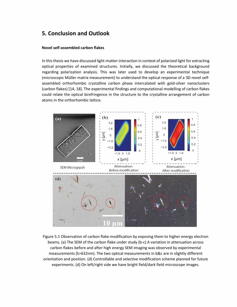
5. Conclusion and Outlook
Novel self-assembled carbon flakes
In this thesis we have discussed light-matter interaction in context of polarized light for extracting
optical properties of examined structures. Initially, we discussed the theoretical background
regarding polarization analysis. This was later used to develop an experimental technique
(microscopic Müller matrix measurement) to understand the optical response of a 3D novel self-
assembled orthorhombic crystalline carbon phase intercalated with gold-silver nanoclusters
(carbon flakes) [14, 18]. The experimental findings and computational modelling of carbon flakes
could relate the optical birefringence in the structure to the crystalline arrangement of carbon
atoms in the orthorhombic lattice.
Figure 5.1 Observation of carbon flake modification by exposing them to higher energy electron
beams. (a) The SEM of the carbon flake under study (b-c) A variation in attenuation across
carbon flakes before and after high energy SEM imaging was observed by experimental
measurements (λ=632nm). The two optical measurements in b&c are in slightly different
orientation and position. (d) Controllable and selective modification scheme planned for future
experiments. (d) On left/right side we have bright field/dark field microscope images.

5. Conclusion and Outlook
86
The attenuation in carbon flakes was found to be a direct indication of bimetallic nanoclusters
present in the carbon flake. We also studied the dependence of optical and geometrical properties
of carbon flakes on fabrication parameters [15]. Due to their hybrid organometallic nature, these
self-assembled structures can find applications in the fields of sensing, electronics and plasmonics
[25, 26]. Our study provided ways that can be helpful in the future to fine-tune the optical and
geometrical properties of self-assembled structures for larger scale fabrication. The intriguing
nature of these self-assembled structures demands more investigations, which are planned in the
future. During experimental investigation, it was observed that carbon flakes are sensitive to
external stimuli and could also be modified by exposing them to electron, light, or ion beams. For
instance, a variation in attenuation across carbon flakes before and after high energy SEM imaging
(Figure 5.1a) was observed by experimental optical measurements (λ=632nm), as shown in Figure
5.1b and c. The two optical measurements in b&c are in slightly different orientation and position.
This modification can also be locally induced on flakes in a selective manner by controlling the
exposure of high energy on the flakes’ surface. As a proof of concept, a focused He-ion beam with
energies ranging up to 30keV was used to locally modify flakes, as shown in Figure 5.1d. In a next
step, a similar experimental examination of optical properties, as discussed in Chapter 3, will be
performed to understand the effects of such modifications. This selective and controllable
modification could be valuable in the future to selectively control the routing of light and for
sensing applications by applying said modifications. During the fabrication process, carbon flake
growth was also found to selectively favor regions on the substrates featuring epitaxially grown
graphene as compared to silicon carbide (SiC). This might pave the wave for selective growth of
flakes in desired regions of interest, acting as sensing pads for surface enhanced Raman
measurements [25, 26].
Furthermore, an initial study for understanding the conductivity of carbon flakes was performed
at the Institute of Applied Physics, University of Erlangen-Nuremberg. The study indicated a highly
insulating behavior also confirming a highly crystalline structure. A Kelvin probe force microscopic
measurement suggested a diode like behavior at the flake-electrode interface. The diode-like
behavior along with other factors could explain the insulation behavior found in the carbon flakes
[262].
Due to sensitive nature of carbon flakes and the large crystalline unit cell, the exact position of
carbon atoms within the unit cell is still not completely known. Currently, rigorous efforts are
being made to comprehend the underlying chemical mechanism, which helps unfold the
intriguing features of this structure.
Brewster effect based refractive index retrieval
We discussed and implemented the High NA focusing objective based refractive index retrieval
technique, which was tested on dielectric, absorbing and uniaxial crystalline structures besides
carbon flakes. The measurement system provided us with a preliminary estimate of complex
refractive indices of carbon flake. The results shown in Section 3.3.5 were mainly performed using
linearly polarized input beam. This technique could be useful in the future for extracting the local
refractive index information in smaller focal spots (in order of hundreds of nanometers) as
compared to existing commercial solutions (in order of tens of microns). One instance is the
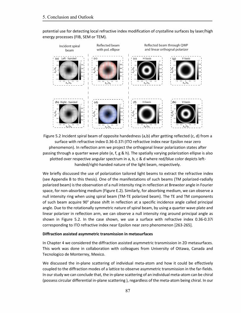
5. Conclusion and Outlook
87
potential use for detecting local refractive index modification of crystalline surfaces by laser/high
energy processes (FIB, SEM or TEM).
Figure 5.2 Incident spiral beam of opposite handedness (a,b) after getting reflected (c, d) from a
surface with refractive index 0.36-0.37i (ITO refractive index near Epsilon near zero
phenomenon). In reflection arm we project the orthogonal linear polarization states after
passing through a quarter wave plate (e, f, g & h). The spatially varying polarization ellipse is also
plotted over respective angular spectrum in a, b, c & d where red/blue color depicts left-
handed/right-handed nature of the light beam, respectively.
We briefly discussed the use of polarization tailored light beams to extract the refractive index
(see Appendix B to this thesis). One of the manifestations of such beams (TM polarized-radially
polarized beam) is the observation of a null intensity ring in reflection at Brewster angle in Fourier
space, for non-absorbing medium (Figure E.2). Similarly, for absorbing medium, we can observe a
null intensity ring when using spiral beam (TM-TE polarized beam). The TE and TM components
of such beam acquire 90° phase shift in reflection at a specific incidence angle called principal
angle. Due to the rotationally symmetric nature of spiral beam, by using a quarter wave plate and
linear polarizer in reflection arm, we can observe a null intensity ring around principal angle as
shown in Figure 5.2. In the case shown, we use a surface with refractive index 0.36-0.37i
corresponding to ITO refractive index near Epsilon near zero phenomenon [263-265].
Diffraction assisted asymmetric transmission in metasurfaces
In Chapter 4 we considered the diffraction assisted asymmetric transmission in 2D metasurfaces.
This work was done in collaboration with colleagues from University of Ottawa, Canada and
Tecnologico de Monterrey, Mexico.
We discussed the in-plane scattering of individual meta-atom and how it could be effectively
coupled to the diffraction modes of a lattice to observe asymmetric transmission in the far-fields.
In our study we can conclude that, the in-plane scattering of an individual meta-atom can be chiral
(possess circular differential in-plane scattering ), regardless of the meta-atom being chiral. In our
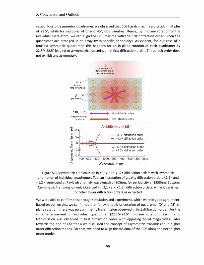
5. Conclusion and Outlook
88
case of fourfold symmetric quadrumer, we observed that CDS has its maxima along odd multiples
of 22.5°, while for multiples of 0° and 45°, CDS vanishes. Hence, by in-plane rotation of the
individual meta-atom, we can align the CDS maxima with the first diffraction order, when the
quadrumer are arranged in an array (with specific periodicity). As evident, for our case of a
fourfold symmetric quadrumer, this happens for an in-plane rotation of each quadrumer by
22.5°/-22.5° leading to asymmetric transmission in first diffraction order. The zeroth order does
not exhibit any asymmetry.
Figure 5.3 Asymmetric transmission in <2,1> and <1,2> diffraction orders with symmetric
orientation of individual quadrumer. Top: an illustration of grazing diffraction orders <2,1> and
<1,2> generated at Rayleigh anomaly wavelength of 905nm, for periodicity of 1350nm. Bottom:
Asymmetric transmission only observed in <2,1> and <1,2> diffraction orders, while it vanishes
for other lower diffraction orders as expected.
We were able to confirm this through simulation and experiment, which were in good agreement.
Based on our results, we confirmed that for symmetric orientation of quadrumer (0° and 45° in-
plane rotation) there was no asymmetric transmission observed in first diffraction order. For the
chiral arrangement of individual quadrumer (22.5°/-22.5° in-plane rotation), asymmetric
transmission was observed in first diffraction order with opposing equal magnitudes. Later
towards the end of Chapter 4 we discussed the concept of asymmetric transmission in higher
order diffraction modes. For that, we need to align the maxima of the CDS along the next higher
order mode.
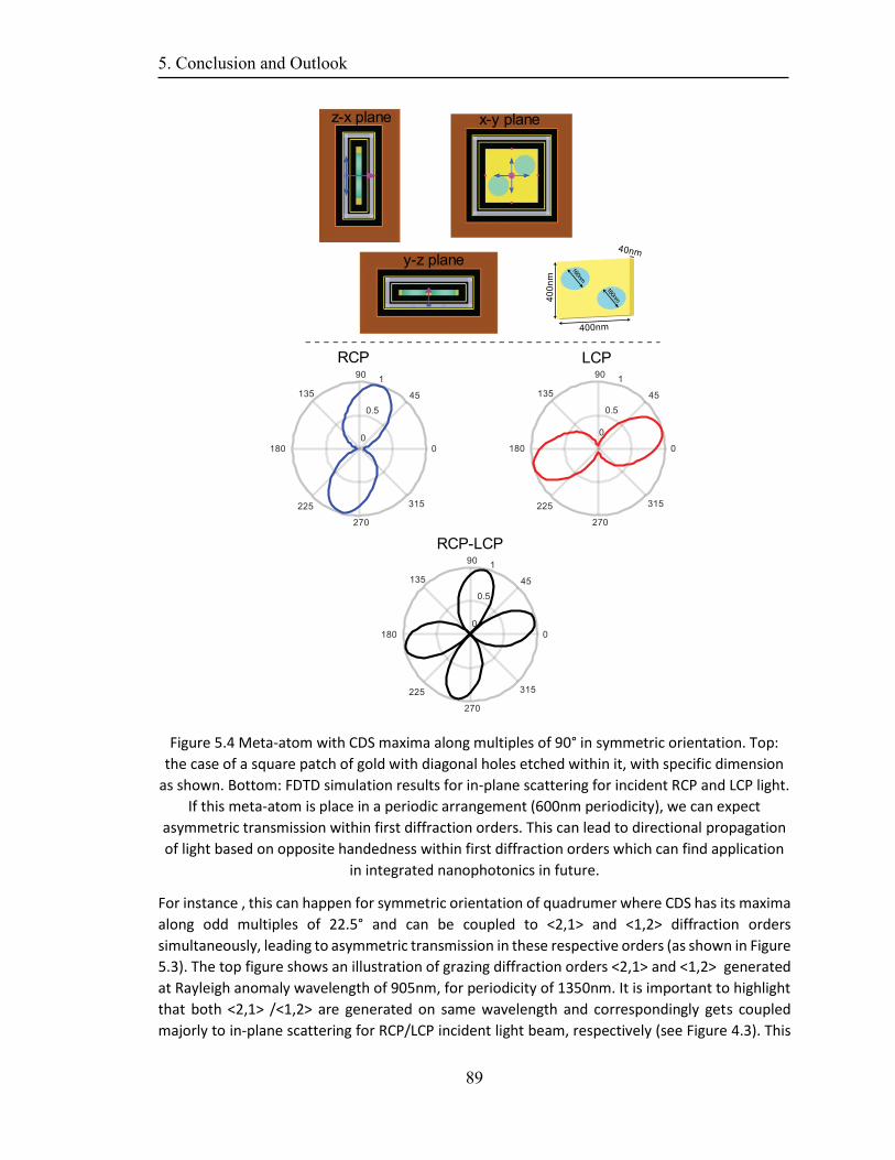
5. Conclusion and Outlook
89
Figure 5.4 Meta-atom with CDS maxima along multiples of 90° in symmetric orientation. Top:
the case of a square patch of gold with diagonal holes etched within it, with specific dimension
as shown. Bottom: FDTD simulation results for in-plane scattering for incident RCP and LCP light.
If this meta-atom is place in a periodic arrangement (600nm periodicity), we can expect
asymmetric transmission within first diffraction orders. This can lead to directional propagation
of light based on opposite handedness within first diffraction orders which can find application
in integrated nanophotonics in future.
For instance , this can happen for symmetric orientation of quadrumer where CDS has its maxima
along odd multiples of 22.5° and can be coupled to <2,1> and <1,2> diffraction orders
simultaneously, leading to asymmetric transmission in these respective orders (as shown in Figure
5.3). The top figure shows an illustration of grazing diffraction orders <2,1> and <1,2> generated
at Rayleigh anomaly wavelength of 905nm, for periodicity of 1350nm. It is important to highlight
that both <2,1> /<1,2> are generated on same wavelength and correspondingly gets coupled
majorly to in-plane scattering for RCP/LCP incident light beam, respectively (see Figure 4.3). This
5. Conclusion and Outlook
90
leads to AT with opposing equal magnitudes (see Figure 5.3 bottom part) in these diffraction
orders.
Therefore, unlike the case of AT in chiral orientation discussed above (and in chapter 4), for
symmetric orientation.in total transmission AT vanishes, although present in higher diffraction
orders. This argument/concept can lead in future to study some interesting phenomenon such
as AT in higher diffraction orders (<2,1> and <1,2>) for rotationally symmetric structures like
cylinders. Our initial assessment (FDTD simulations for cylinder with 40nm height and 200nm
diameter) shows promising results.
Similarly, we looked into the concept of designing meta-atom, that can generate CDS maxima
along multiples of 90° in symmetric orientation. Thus, leading to asymmetric transmission in first
diffraction orders when placed in an array (with specific periodicity). As an example, we discuss
the case of a square patch of gold with diagonal holes etched within it as shown in top part of
Figure 5.4. The lower part of Figure 5.4 shows FDTD simulation results for in-plane scattering for
incident RCP and LCP light. If this meta-atom is placed in a periodic arrangement (600nm
periodicity), we can expect asymmetric transmission within first diffraction orders. Whereby, the
first diffraction orders along vertical and horizontal direction get resonantly coupled to RCP and
LCP incident light, respectively. This can lead to directional propagation of light based on opposite
handedness within first diffraction orders which can find application in integrated nanophotonics
in future.
To conclude, the studies presented in this thesis, demonstrate the advantage and versatility of
studying of light-mater interaction exploiting polarization state of light. We used various
experimental systems to devise ways and methods to study intriguing optical phenomena at small
scales. Most of the studies were performed in collaboration with researchers across the globe
belonging from different fields of science. This helped us in understanding novel structures and
metasurfaces in a more comprehensive way, leading to ideas and concepts for future projects.
A. Some mathematical relations
Circularly polarized light and chirality
Light waves can carry angular momentum and exert torque on surfaces/media they are
interacting with in two distinct ways [266, 267]. The spin (𝜎) and orbital (𝑙) angular momentum,
which involve polarization and spatial wavefront/phase profile of light wave, respectively. We will
keep our discussion here to spin angular momentum (SAM) as it is related to polarization states
of light. Mathematically this can be written as
𝜏 =𝜎
2𝜋𝜈=
𝜎
𝜔, (A.1)
Hence, SAM carried per photon can be represented as 𝜎ћ. Right-handed circularly polarized
paraxial light beams therefore carry SAM in the direction parallel to propagation direction (𝜎 =
−1), while for left circularly polarized it is in the opposite direction (𝜎 = 1). Linear states of
polarization can be thought of as containing equal right and left circular contributions and hence
total SAM is equal zero. Circularly polarized light propagating along a certain direction spins with
time or in space about the optical axis in a helical fashion [66]. This intriguing phenomenon has
an analog in terms of optical properties of a medium, i.e., the chirality or optical activity [67].
Optical activity and reciprocity
The optical phenomenon of circular retardance together with circular dichroism are often named
as optical activity [268]. Circular dichroism results in differential extinction for incoming circularly
polarized light. While circular retardance rotates the azimuthal angle of the incoming polarization,
proportional to retardance while it does not affect the ellipticity of the light wave (incoming
circular polarization is preserved). This effect is somewhat similar to optical rotation effect
observed by the Faraday [223] in the presence of a static magnetic field but with one distinction,
i.e., reciprocity. The earliest work regarding reciprocity in optics was done by G. G. Stokes and
Helmholtz around 1850s. Lord Kelvin, Kirchhoff and Rayleigh also mentioned similar concepts of
reciprocity in fields the of thermoelectric, thermal radiation and acoustics, respectively [231].
Later H. Lorentz formulated the electromagnetic reciprocity theorem. Mathematically, by
considering two spatially separate volumes with certain current densities, we perform divergence
operation on Maxwell’s curl equations. Resultantly, we end up with Lorentz reciprocity theorem
with sources,
𝛁. (𝑬𝟏 × 𝑯𝟐 − 𝑬𝟐 × 𝑯𝟏) = 𝒋𝟏. 𝑬𝟐 − 𝒋𝟐. 𝑬𝟏. (A.2)
In terms of discussion regarding Faraday effect, it is important to remember that circular
dichroism and circular retardance are reciprocal quantities. On the other hand, Faraday effect is
non-reciprocal and depends on the direction of light propagation in relation to that of magnetic
field, hence producing vanishing chiral effects.
A. Some mathematical relations
92
Relation between Jones and Müller matrix
Since both Jones and Müller formalism deal with polarized light-matter interaction, extensive
research has been done to mathematically relate both matrices [84, 96]. Since, Jones formalism
does not deal with partially polarized light, therefore usually the first step involves removing
depolarization information from Müller matrix [95]. Later, a Müller matrix and its corresponding
Jones matrix can be related by the equation,
𝑀 = 𝐴(𝐽 ⊗ 𝐽∗)𝐴−1 also, 𝑚𝑖𝑗 =1
2𝑇𝑟(𝐽𝜎𝑖𝐽
†𝜎𝑗) ∈ 𝑖, 𝑗 = 0,1,2,3, (A.3)
𝐴 = [
1 0 0 11 0 0 −10 1 1 00 −𝑖 𝑖 0
], (A.4)
where ⊗ denotes the Kronecker product , 𝜎 is an individual Pauli matrix and A is a combination
of 3 Pauli matrices and 2x2 unitary matrix [56]. The origin of this elegant connection to Pauli
matrices lies in the concept of coherency matrices which is another way to describe polarized
light, introduced by Soleillit, Weiner and later reintroduced by E. Wolf [56, 87]. The 2x2 coherency
matrix is based on correlations between orthogonal field components of a light wave under
consideration. In fact, the field relations shown in Equation 2.33 define the elements of a
coherency matrix. The decomposition relation between coherency matrix and Stokes vector lies
in Pauli matrices, which was first Figured out by U. Fano in 1954 [269]. It is pertinent to highlight
that similar to 2x2 Pauli matrices, the linearly independent nine, 3x3 Hermitian matrices (also
known as Gell-Mann matrices [270]) can be used to define arbitrary polarized light wave in three
dimensions [80, 271, 272].
Brewster effect in uniaxial crystals
As discussed in section 2.3.1, materials which show birefringence has varying refractive indices
along their principal axis. In following we will discuss such cases and how anisotropy affects the
Brewster angle of the material.
Following from Equation 2.21a&b, we can expand constitutive relations to accommodate more
generalized solutions where the permittivity and permeability can be defined as 3 dimensional
tensors. Mathematically we can expect it to take the following form [273]
휀 = [
휀𝑥𝑥 0 00 휀𝑦𝑦 0
00 0 휀𝑧𝑧
], (A.5)
where, 휀𝑥𝑥 , 휀𝑦𝑦 & 휀𝑧𝑧 are the permittivity tensors along three principal axes of a medium [98,
273]. Intuitively, we can expect cases in which diagonal tensor elements all are identical
(isotropic), two are identical (uniaxial) or all three different (biaxial). Extending on Brewster effect
for a medium, we can discuss this effect in relation to uniaxial systems [75]. For a uniaxial crystal
in the dielectric case (no absorption in medium) two refractive indices are defined as ordinary 𝑛0
and extraordinary 𝑛𝑒. The refractive index of incident medium is denoted as 𝑛1 [75, 81]. Following
the existing mathematical notation [75], we can distinguish three cases:
A. Some mathematical relations
93
Case 1: Surface parallel to optic axis, with optic axis pointing normal to the plane of incidence. In
this case, the light wave sees only the ordinary refractive index and hence can be written in a
similar way as for an isotropic medium:
𝑏1 = tan𝜃𝐵1 =𝑛0
𝑛1. (A.6a)
Case 2: A Surface that is parallel to the optic axis, with optic axis being parallel to the plane of
incidence. In this case we expect a cross combination of ordinary and extraordinary refractive
indices and corresponding contributions to the effect at the Brewster angle
𝑏2 = sin2 𝜃𝐵2 =𝑛1
2𝑛𝑜2−𝑛𝑜
2𝑛𝑒2
𝑛14−𝑛𝑜
2𝑛𝑒2 . (A.6b)
These two cases are of more experimental importance and will be discussed later in the
experimental part.
Case 3: For a surface normal to the optic axis, we can define the Brewster angle as
𝑏3 = sin2 𝜃𝐵3 =𝑛1
2𝑛𝑒2−𝑛𝑜
2𝑛𝑒2
𝑛14−𝑛𝑜
2𝑛𝑒2 . (A.6c)
For example, taking the case of rutile (titanium dioxide in its natural crystalline form), the two
refractive indices are 𝑛0 = 1.6557 and 𝑛𝑒 = 1.4849 and we get 𝜃𝐵1 = 58.870°, 𝜃𝐵2 = 54.01°
and 𝜃𝐵3 = 60.7°.
Brewster effect in Biaxial Crystal
Following from Equation A.5, the case of a uniaxial crystal can be further extended to the biaxial
crystal case in similar manner. We can expect for a biaxial crystal a total of 12 Brewster angle
cases which, due to symmetry, are reduced to 6 unique Brewster angles [75, 121].
𝑏1 = sin2 𝜃𝛽′ =𝑛1
2𝑛𝑧2+𝑛𝑥
2𝑛𝑧2
𝑛12−𝑛𝑥
2𝑛𝑧2 , (A.7a)
𝑏2 = sin2 𝜃𝛽′ =𝑛1
2𝑛𝑧2+𝑛𝑦
2𝑛𝑧2
𝑛12−𝑛𝑦
2𝑛𝑧2 , (A.7b)
𝑏3 = sin2 𝜃𝛽′ =𝑛1
2𝑛𝑦2+𝑛𝑥
2𝑛𝑦2
𝑛12−𝑛𝑥
2𝑛𝑦2 , (A.7c)
𝑏4 = sin2 𝜃𝛽′ =𝑛1
2𝑛𝑦2+𝑛𝑧
2𝑛𝑦2
𝑛12−𝑛𝑧
2𝑛𝑦2 , (A.7d)
𝑏5 = sin2 𝜃𝛽′ =𝑛1
2𝑛𝑥2+𝑛𝑦
2𝑛𝑥2
𝑛12−𝑛𝑦
2𝑛𝑥2 , (A.7e)
𝑏6 = sin2 𝜃𝛽′ =𝑛1
2𝑛𝑥2+𝑛𝑧
2𝑛𝑥2
𝑛12−𝑛𝑧
2𝑛𝑥2 . (A.7f)
For instance, we compare the equations with experimental results for biaxial organic crystal MNA
(2-methyl-4-nitroaniline) [121].The three of the Brewster angles observed in the case of above-
mentioned experimental study, matches the estimates (𝑏2 = 65.1212°, 𝑏3 = 71.8603°, 𝑏4 =
51.7114°) observed by us, using analytical equations.
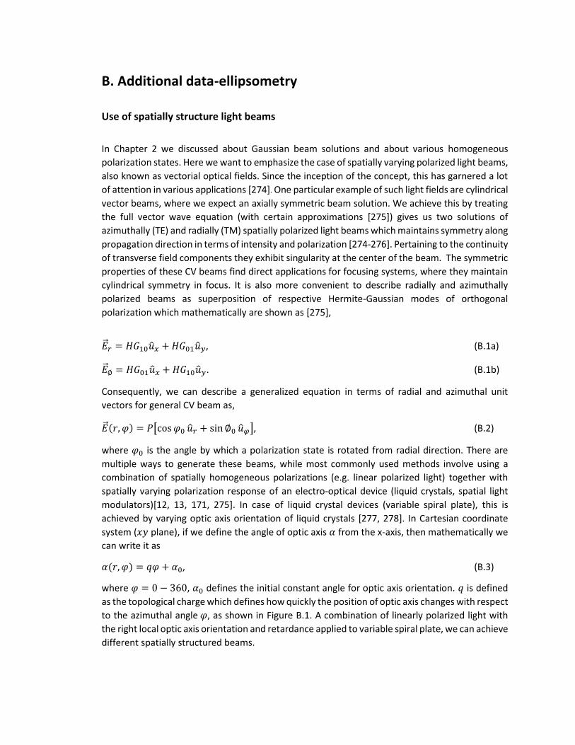
B. Additional data-ellipsometry
Use of spatially structure light beams
In Chapter 2 we discussed about Gaussian beam solutions and about various homogeneous
polarization states. Here we want to emphasize the case of spatially varying polarized light beams,
also known as vectorial optical fields. Since the inception of the concept, this has garnered a lot
of attention in various applications [274]. One particular example of such light fields are cylindrical
vector beams, where we expect an axially symmetric beam solution. We achieve this by treating
the full vector wave equation (with certain approximations [275]) gives us two solutions of
azimuthally (TE) and radially (TM) spatially polarized light beams which maintains symmetry along
propagation direction in terms of intensity and polarization [274-276]. Pertaining to the continuity
of transverse field components they exhibit singularity at the center of the beam. The symmetric
properties of these CV beams find direct applications for focusing systems, where they maintain
cylindrical symmetry in focus. It is also more convenient to describe radially and azimuthally
polarized beams as superposition of respective Hermite-Gaussian modes of orthogonal
polarization which mathematically are shown as [275],
�� 𝑟 = 𝐻𝐺10��𝑥 + 𝐻𝐺01��𝑦, (B.1a)
�� ∅ = 𝐻𝐺01��𝑥 + 𝐻𝐺10��𝑦. (B.1b)
Consequently, we can describe a generalized equation in terms of radial and azimuthal unit
vectors for general CV beam as,
�� (𝑟, 𝜑) = 𝑃[cos𝜑0 ��𝑟 + sin∅0 ��𝜑], (B.2)
where 𝜑0 is the angle by which a polarization state is rotated from radial direction. There are
multiple ways to generate these beams, while most commonly used methods involve using a
combination of spatially homogeneous polarizations (e.g. linear polarized light) together with
spatially varying polarization response of an electro-optical device (liquid crystals, spatial light
modulators)[12, 13, 171, 275]. In case of liquid crystal devices (variable spiral plate), this is
achieved by varying optic axis orientation of liquid crystals [277, 278]. In Cartesian coordinate
system (𝑥𝑦 plane), if we define the angle of optic axis 𝛼 from the x-axis, then mathematically we
can write it as
𝛼(𝑟, 𝜑) = 𝑞𝜑 + 𝛼0, (B.3)
where 𝜑 = 0 − 360, 𝛼0 defines the initial constant angle for optic axis orientation. 𝑞 is defined
as the topological charge which defines how quickly the position of optic axis changes with respect
to the azimuthal angle 𝜑, as shown in Figure B.1. A combination of linearly polarized light with
the right local optic axis orientation and retardance applied to variable spiral plate, we can achieve
different spatially structured beams.
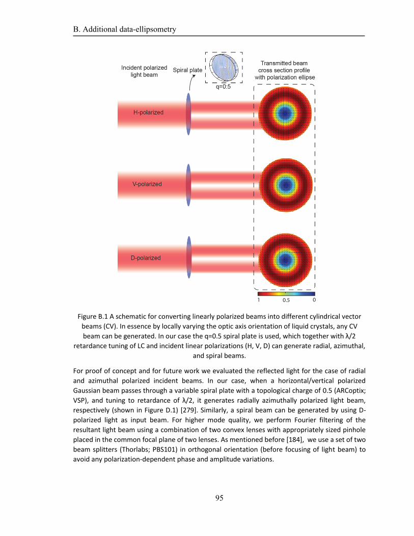
B. Additional data-ellipsometry
95
Figure B.1 A schematic for converting linearly polarized beams into different cylindrical vector
beams (CV). In essence by locally varying the optic axis orientation of liquid crystals, any CV
beam can be generated. In our case the q=0.5 spiral plate is used, which together with λ/2
retardance tuning of LC and incident linear polarizations (H, V, D) can generate radial, azimuthal,
and spiral beams.
For proof of concept and for future work we evaluated the reflected light for the case of radial
and azimuthal polarized incident beams. In our case, when a horizontal/vertical polarized
Gaussian beam passes through a variable spiral plate with a topological charge of 0.5 (ARCoptix;
VSP), and tuning to retardance of λ/2, it generates radially azimuthally polarized light beam,
respectively (shown in Figure D.1) [279]. Similarly, a spiral beam can be generated by using D-
polarized light as input beam. For higher mode quality, we perform Fourier filtering of the
resultant light beam using a combination of two convex lenses with appropriately sized pinhole
placed in the common focal plane of two lenses. As mentioned before [184], we use a set of two
beam splitters (Thorlabs; PBS101) in orthogonal orientation (before focusing of light beam) to
avoid any polarization-dependent phase and amplitude variations.
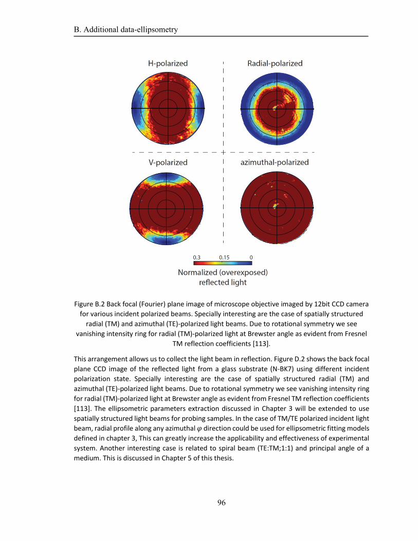
B. Additional data-ellipsometry
96
Figure B.2 Back focal (Fourier) plane image of microscope objective imaged by 12bit CCD camera
for various incident polarized beams. Specially interesting are the case of spatially structured
radial (TM) and azimuthal (TE)-polarized light beams. Due to rotational symmetry we see
vanishing intensity ring for radial (TM)-polarized light at Brewster angle as evident from Fresnel
TM reflection coefficients [113].
This arrangement allows us to collect the light beam in reflection. Figure D.2 shows the back focal
plane CCD image of the reflected light from a glass substrate (N-BK7) using different incident
polarization state. Specially interesting are the case of spatially structured radial (TM) and
azimuthal (TE)-polarized light beams. Due to rotational symmetry we see vanishing intensity ring
for radial (TM)-polarized light at Brewster angle as evident from Fresnel TM reflection coefficients
[113]. The ellipsometric parameters extraction discussed in Chapter 3 will be extended to use
spatially structured light beams for probing samples. In the case of TM/TE polarized incident light
beam, radial profile along any azimuthal 𝜑 direction could be used for ellipsometric fitting models
defined in chapter 3, This can greatly increase the applicability and effectiveness of experimental
system. Another interesting case is related to spiral beam (TE:TM;1:1) and principal angle of a
medium. This is discussed in Chapter 5 of this thesis.
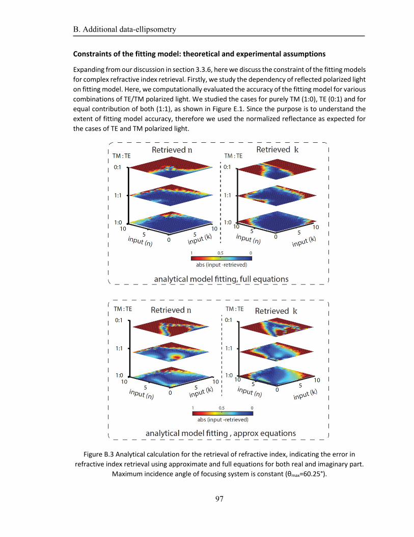
B. Additional data-ellipsometry
97
Constraints of the fitting model: theoretical and experimental assumptions
Expanding from our discussion in section 3.3.6, here we discuss the constraint of the fitting models
for complex refractive index retrieval. Firstly, we study the dependency of reflected polarized light
on fitting model. Here, we computationally evaluated the accuracy of the fitting model for various
combinations of TE/TM polarized light. We studied the cases for purely TM (1:0), TE (0:1) and for
equal contribution of both (1:1), as shown in Figure E.1. Since the purpose is to understand the
extent of fitting model accuracy, therefore we used the normalized reflectance as expected for
the cases of TE and TM polarized light.
Figure B.3 Analytical calculation for the retrieval of refractive index, indicating the error in
refractive index retrieval using approximate and full equations for both real and imaginary part.
Maximum incidence angle of focusing system is constant (θmax=60.25°).
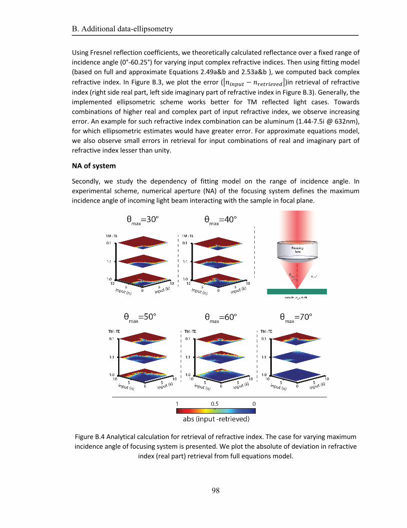
B. Additional data-ellipsometry
98
Using Fresnel reflection coefficients, we theoretically calculated reflectance over a fixed range of
incidence angle (0°-60.25°) for varying input complex refractive indices. Then using fitting model
(based on full and approximate Equations 2.49a&b and 2.53a&b ), we computed back complex
refractive index. In Figure B.3, we plot the error (|𝑛𝑖𝑛𝑝𝑢𝑡 − 𝑛𝑟𝑒𝑡𝑟𝑖𝑒𝑣𝑒𝑑|)in retrieval of refractive
index (right side real part, left side imaginary part of refractive index in Figure B.3). Generally, the
implemented ellipsometric scheme works better for TM reflected light cases. Towards
combinations of higher real and complex part of input refractive index, we observe increasing
error. An example for such refractive index combination can be aluminum (1.44-7.5i @ 632nm),
for which ellipsometric estimates would have greater error. For approximate equations model,
we also observe small errors in retrieval for input combinations of real and imaginary part of
refractive index lesser than unity.
NA of system
Secondly, we study the dependency of fitting model on the range of incidence angle. In
experimental scheme, numerical aperture (NA) of the focusing system defines the maximum
incidence angle of incoming light beam interacting with the sample in focal plane.
Figure B.4 Analytical calculation for retrieval of refractive index. The case for varying maximum
incidence angle of focusing system is presented. We plot the absolute of deviation in refractive
index (real part) retrieval from full equations model.
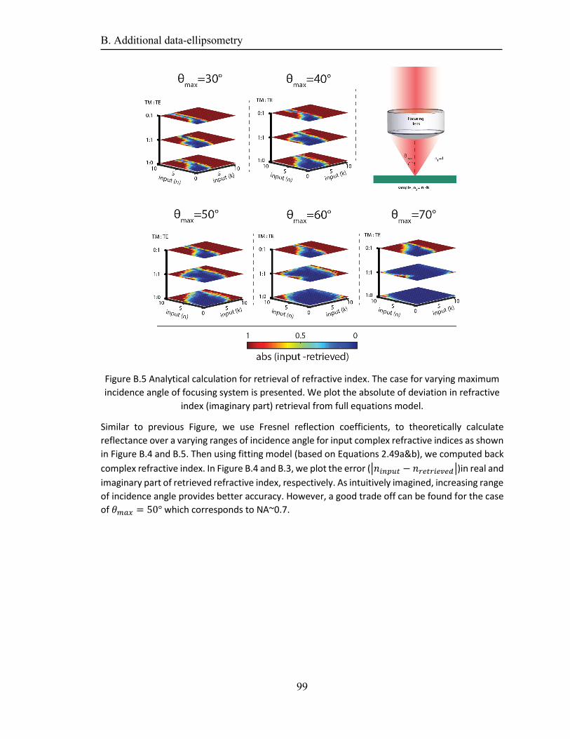
B. Additional data-ellipsometry
99
Figure B.5 Analytical calculation for retrieval of refractive index. The case for varying maximum
incidence angle of focusing system is presented. We plot the absolute of deviation in refractive
index (imaginary part) retrieval from full equations model.
Similar to previous Figure, we use Fresnel reflection coefficients, to theoretically calculate
reflectance over a varying ranges of incidence angle for input complex refractive indices as shown
in Figure B.4 and B.5. Then using fitting model (based on Equations 2.49a&b), we computed back
complex refractive index. In Figure B.4 and B.3, we plot the error (|𝑛𝑖𝑛𝑝𝑢𝑡 − 𝑛𝑟𝑒𝑡𝑟𝑖𝑒𝑣𝑒𝑑|)in real and
imaginary part of retrieved refractive index, respectively. As intuitively imagined, increasing range
of incidence angle provides better accuracy. However, a good trade off can be found for the case
of 𝜃𝑚𝑎𝑥 = 50° which corresponds to NA~0.7.

C Additional data-quadrumer array
In the course of this thesis, we tried different combinations of focusing lens to study quadrumer
array samples. Although, for the evaluation of asymmetric transmission we used low NA focusing
lens as mentioned in section 3.4., here we will discuss the case of high NA focusing objective (NA
0.9). This would essentially correspond to a focal spot of approximately 1.5microns near Rayleigh
anomaly for first diffraction order (𝜆𝑅𝐴 = 905𝑛𝑚. We use the experimental setup as described in
section 4.2, except the interchanging of high NA focusing objective (shown in Figure C.1).
Figure C.1 Probing quadrumer array sample near Rayleigh anomaly for first diffraction order
(𝜆𝑅𝐴 = 905𝑛𝑚) with high NA (0.9) focusing objective. We use the experimental setup as
described in section 4.2, except the interchanging of high NA focusing objective (shown in Figure
F.1). We plot the BFP images recorded near Rayleigh anomaly for two chiral orientations of
quadrumer (22.5°& -22.5°). These BFP images are also superimposed with simulated in-plane
scattering of individual quadrumer for certain incident handedness of light beam (RCP for -22.5
and LCP for 22.5°). we concentrate on the first diffraction orders in the BFP which are present in
the region 1.3<NA>0.9, hence we omit the central region of the BFP image (NA<0.9).
C Additional data-quadrumer array
101
The quadrumer array was precisely positioned in the focal spot with help of 3-axis piezo stage. An
oil-immersion microscope objective (NA 1.3) was then used to collect the transmitted light as
shown in Figure C.1. The back focal plane (BFP) of this microscope objective is imaged onto a 12
bit CCD-camera [172], using a single achromatic lens (f=300mm) which helps us to angularly
resolve the transmitted light. In the right side of Figure C.1 we plot the BFP images recorded near
Rayleigh anomaly for two chiral orientations of quadrumer (22.5°& -22.5°). These BFP images are
also superimposed with simulated in-plane scattering of individual quadrumer for certain incident
handedness of light beam (RCP for -22.5 and LCP for 22.5°). We concentrate on the first diffraction
orders in the BFP which are present in the region 1.3<NA>0.9, hence we omit the central region
of the BFP image (NA<0.9). As we can observe, within each first diffraction order in BFP image, we
observe regions of high and low intensity. The regions of high intensity coincide well with the in-
plane scattering of individual quadrumer of certain handedness. The difference in high and low
intensity regions could also correspond to asymmetric transmission. However, this technique (in
present state) provided more of a qualitative analysis, rather a quantitative one, hence was not
used for further analysis.
References
[1] M. Berger, "Nanotechnology : the future is tiny," (in English), 2016. [2] B. Bhushan, Springer handbook of nanotechnology. Springer, 2017. [3] J. M. Lourtioz and S. N. Lyle, Nanosciences and nanotechnology : evolution or revolution? (in
English), 2016. [4] E. Regis, Nano : the emerging science of nanotechnology : remaking the world-molecule by
molecule. Boston: Little, Brown (in English), 1995. [5] R. Waser, Nanoelectronics and information technology. Wiley Online Library, 2003. [6] E. L. Wolf, "Nanophysics and nanotechnology," Wiley-VCH, Weinheim. DOI, vol. 10, no. 978352761,
p. 8972, 2004. [7] L. Novotny and B. Hecht, Principles of Nano-Optics. Cambridge University Press, 2006. [8] J. Weiner and F. Nunes, Light-matter interaction: physics and engineering at the nanoscale. Oxford
University Press, 2017. [9] C. Lienau, M. A. Noginov, M. Lončar, C. Bauer, and H. Giessen, "Light–matter interactions at the
nanoscale," J. Opt, vol. 16, no. 110201, p. 110201, 2014. [10] P. Banzer, " Anregung einzelner Nanostrukturen mit hochfokussierten Vektorfeldern," riedrich-
Alexander-University Erlangen-Nürnberg, Erlangen, 2012. [11] P. Woźniak, "Light-matter Interactions with Polarization-tailored Fields," Friedrich-Alexander-
Universität Erlangen-Nürnberg, 2018. [12] M. Neugebauer, "Transverse Spin in Structured Light," Friedrich-Alexander-Universität Erlangen-
Nürnberg, 2018. [13] T. Bauer, "Probe-based nano-interferometric reconstruction of tightly focused vectorial light
fields," 2017. [14] M. A. Butt et al., "Investigating the Optical Properties of a Laser Induced 3D Self-Assembled
Carbon-Metal Hybrid Structure," Small, vol. 15, no. 18, p. e1900512, May 2019, doi: 10.1002/smll.201900512.
[15] M. A. Butt et al., "Hybrid Orthorhombic Carbon Flakes Intercalated with Bimetallic Au-Ag Nanoclusters: Influence of Synthesis Parameters on Optical Properties," Nanomaterials (Basel), vol. 10, no. 7, Jul 15 2020, doi: 10.3390/nano10071376.
[16] N. A. Chaitanya, M. A. Butt, O. Reshef, R. W. Boyd, P. Banzer, and I. D. Leon1, "Diffraction assisted chiral scattering for 2D metasurfaces (in progress)," 2021.
[17] R. Barczyk, S. Nechayev, M. A. Butt, G. Leuchs, and P. Banzer, "Vectorial vortex generation and phase singularities upon Brewster reflection," Physical Review A, vol. 99, no. 6, p. 063820, 2019.
[18] A. Butt et al., "Investigating the Optical Properties of a Novel 3D Self-Assembled Metamaterial made of Carbon Intercalated with Bimetal Nanoparticles," in OSA Advance Photonics, Zurich, 2018.
[19] M. A. Butt, D. Mamonova, A. A. Manshina, P. Banzer, and G. Leuchs, "Tuning the Optical and Geometrical Properties of Hybrid Carbon Flakes by Fabrication Parameters," in OSA Advanced Photonics Congress (AP) 2020 (IPR, NP, NOMA, Networks, PVLED, PSC, SPPCom, SOF), Washington, DC, L. T.-P. A. L. F. Caspani and B. Yang, Eds., 2020/07/13 2020: Optical Society of America, in OSA Technical Digest, p. JTu4C.14, doi: 10.1364/NOMA.2020.JTu4C.14.
[20] A. Manshina et al., "2D carbon allotrope with incorporated Au-Ag nanoclusters – Laser-induced synthesis and optical characterization," in CLEO Pacific Rim Conference 2018, Hong Kong, 2018/07/29 2018: Optical Society of America, in OSA Technical Digest, p. Th1G.2, doi: 10.1364/CLEOPR.2018.Th1G.2.
[21] A. Manshina, T. Ivanova, and A. Povolotskiy, "Laser-induced deposition of hetero-metallic structures from liquid phase," (in English), Laser Physics, vol. 20, no. 6, pp. 1532-1536, Jun 2010, doi: 10.1134/s1054660x10110162.
[22] A. Manshina et al., "Novel 2D carbon allotrope intercalated with Au-Ag nanoclusters. From laser design to functionality," in Advance Photonics 2017, New Orleans, Louisiana 70130, 2017.
References
103
[23] A. A. Manshina et al., "Laser-induced transformation of supramolecular complexes: approach to controlled formation of hybrid multi-yolk-shell Au-Ag@a-C:H nanostructures," (in English), Sci Rep, vol. 5, p. 12027, Jul 8 2015, doi: 10.1038/srep12027.
[24] A. Povolotckaia et al., "Plasmonic carbon nanohybrids from laser-induced deposition: controlled synthesis and SERS properties," (in English), Journal of Materials Science, vol. 54, no. 11, pp. 8177-8186, Jun 2019, doi: 10.1007/s10853-019-03478-9.
[25] M. Y. Bashouti et al., "Direct laser writing of mu-chips based on hybrid C-Au-Ag nanoparticles for express analysis of hazardous and biological substances," Lab Chip, vol. 15, no. 7, pp. 1742-7, Apr 7 2015, doi: 10.1039/c4lc01376j.
[26] M. Y. Bashouti et al., "Spatially-controlled laser-induced decoration of 2D and 3D substrates with plasmonic nanoparticles," (in English), RSC Advances, vol. 6, no. 79, pp. 75681-75685, 2016, doi: 10.1039/c6ra16585k.
[27] R. Dorn, Polarisationseffekte bei der Fokussierung mit hoher numerischer Apertur. Lehrstuhl für Mikrocharakterisierung, Univ., 2004.
[28] P. Banzer, U. Peschel, S. Quabis, and G. Leuchs, "On the experimental investigation of the electric and magnetic response of a single nano-structure," Opt Express, vol. 18, no. 10, pp. 10905-23, May 10 2010, doi: 10.1364/OE.18.010905.
[29] O. Arteaga, M. Baldris, J. Anto, A. Canillas, E. Pascual, and E. Bertran, "Mueller matrix microscope with a dual continuous rotating compensator setup and digital demodulation," Appl Opt, vol. 53, no. 10, pp. 2236-45, Apr 1 2014, doi: 10.1364/AO.53.002236.
[30] J. M. Bueno, "Polarimetry using liquid-crystal variable retarders: theory and calibration," (in English), Journal of Optics A: Pure and Applied Optics, vol. 2, no. 3, pp. 216-222, May 2000, doi: 10.1088/1464-4258/2/3/308.
[31] O. A. Barriel, "Mueller matrix polarimetry of anisotropic chiral media," Universitat de Barcelona, 2010.
[32] H.-T. Chen, A. J. Taylor, and N. Yu, "A review of metasurfaces: physics and applications," vol. 79, ed, 2016, p. 076401.
[33] J. Pendry and "Metamaterials and the Control of Electromagnetic Fields," ed, 2007, p. CMB2. [34] O. Quevedo-Teruel and e. al., "Roadmap on metasurfaces," vol. 21, ed, 2019, p. 073002. [35] A. Baron, A. Aradian, V. Ponsinet, and P. Barois, "Self-assembled optical metamaterials," Optics &
Laser Technology, vol. 82, pp. 94-100, 2016. [36] W. T. Chen, A. Y. Zhu, and F. Capasso, "Flat optics with dispersion-engineered metasurfaces," vol.
5, ed, 2020, pp. 604-620. [37] H. T. Chen, A. J. Taylor, and N. Yu, "A review of metasurfaces: physics and applications," Rep Prog
Phys, vol. 79, no. 7, p. 076401, Jul 2016, doi: 10.1088/0034-4885/79/7/076401. [38] F. Ding, A. Pors, and S. I. Bozhevolnyi, "Gradient metasurfaces: a review of fundamentals and
applications," Reports on Progress in Physics, vol. 81, no. 2, p. 026401, 2017. [39] T. W. Ebbesen, H. J. Lezec, H. F. Ghaemi, T. Thio, and P. A. Wolff, "Extraordinary optical
transmission through sub-wavelength hole arrays," Nature, vol. 391, no. 6668, pp. 667-669, 1998/02/01 1998, doi: 10.1038/35570.
[40] A. Li, S. Singh, and D. Sievenpiper, "Metasurfaces and their applications," Nanophotonics, vol. 7, no. 6, pp. 989-1011, 2018.
[41] N. Litchinitser and V. Shalaev, "Photonic metamaterials," Laser Physics Letters, vol. 5, no. 6, p. 411, 2008.
[42] J. Pendry, "Metamaterials and the Control of Electromagnetic Fields," ed, 2007, p. CMB2. [43] J. B. Pendry, D. Schurig, and D. R. Smith, "Controlling electromagnetic fields," Science, vol. 312, no.
5781, pp. 1780-2, Jun 23 2006, doi: 10.1126/science.1125907. [44] A. Sihvola, "Metamaterials in electromagnetics," Metamaterials, vol. 1, no. 1, pp. 2-11,
2007/03/01/ 2007, doi: 10.1016/j.metmat.2007.02.003. [45] N. Yu and F. Capasso, "Flat optics with designer metasurfaces," Nat Mater, vol. 13, no. 2, pp. 139-
50, Feb 2014, doi: 10.1038/nmat3839.
References
104
[46] M. Kataja, T. K. Hakala, A. Julku, M. J. Huttunen, S. van Dijken, and P. Torma, "Surface lattice resonances and magneto-optical response in magnetic nanoparticle arrays," Nat Commun, vol. 6, no. 1, p. 7072, May 7 2015, doi: 10.1038/ncomms8072.
[47] A. Abass, S. R.-K. Rodriguez, J. Gomez Rivas, and B. Maes, "Tailoring dispersion and eigenfield profiles of plasmonic surface lattice resonances," ACS Photonics, vol. 1, no. 1, pp. 61-68, 2014.
[48] C. Cherqui, M. R. Bourgeois, D. Wang, and G. C. Schatz, "Plasmonic Surface Lattice Resonances: Theory and Computation," Acc Chem Res, vol. 52, no. 9, pp. 2548-2558, Sep 17 2019, doi: 10.1021/acs.accounts.9b00312.
[49] Z. Li, S. Butun, and K. Aydin, "Ultranarrow band absorbers based on surface lattice resonances in nanostructured metal surfaces," ACS Nano, vol. 8, no. 8, pp. 8242-8, Aug 26 2014, doi: 10.1021/nn502617t.
[50] A. D. Humphrey and W. L. Barnes, "Plasmonic surface lattice resonances on arrays of different lattice symmetry," Physical Review B, vol. 90, no. 7, p. 075404, 2014.
[51] A. Hessel and A. Oliner, "A new theory of Wood’s anomalies on optical gratings," Applied optics, vol. 4, no. 10, pp. 1275-1297, 1965.
[52] V. G. Kravets, A. V. Kabashin, W. L. Barnes, and A. N. Grigorenko, "Plasmonic Surface Lattice Resonances: A Review of Properties and Applications," vol. 118, ed, 2018, pp. 5912-5951.
[53] E. S. A. Goerlitzer et al., "Chiral Surface Lattice Resonances," Adv Mater, vol. 32, no. 22, p. e2001330, Jun 2020, doi: 10.1002/adma.202001330.
[54] V. G. Kravets, A. V. Kabashin, W. L. Barnes, and A. N. Grigorenko, "Plasmonic Surface Lattice Resonances: A Review of Properties and Applications," Chem Rev, vol. 118, no. 12, pp. 5912-5951, Jun 27 2018, doi: 10.1021/acs.chemrev.8b00243.
[55] G. W. Castellanos, P. Bai, and J. Gómez Rivas, "Lattice resonances in dielectric metasurfaces," Journal of Applied Physics, vol. 125, no. 21, p. 213105, 2019.
[56] M. Born et al., Principles of Optics, 7 ed. Cambridge: Cambridge University Press, 2013. [57] E. Wolf, "VIII. A dynamical theory of the electromagnetic field," Philosophical Transactions of the
Royal Society of London, vol. 155, pp. 459-512, 1997, doi: 10.1098/rstl.1865.0008. [58] J. D. Jackson, Classical electrodynamics. Third edition. New York : Wiley, [1999] ©1999, 1999. [59] S. Quabis, R. Dorn, M. Eberler, O. Glöckl, and G. Leuchs, "Focusing light to a tighter spot," Optics
Communications, vol. 179, no. 1-6, pp. 1-7, 2000/05/25/ 2000, doi: 10.1016/s0030-4018(99)00729-4.
[60] N. Rotenberg and L. Kuipers, "Mapping nanoscale light fields," Nature Photonics, vol. 8, no. 12, pp. 919-926, 2014/12/01 2014, doi: 10.1038/nphoton.2014.285.
[61] E. Wolf, "Electromagnetic diffraction in optical systems-I. An integral representation of the image field," Proceedings of the Royal Society of London. Series A. Mathematical and Physical Sciences, vol. 253, no. 1274, pp. 349-357, 1959.
[62] A. B. Vasista, D. K. Sharma, and G. V. P. Kumar, "Fourier Plane Optical Microscopy and Spectroscopy," in digital Encyclopedia of Applied Physics, 2019, pp. 1-14.
[63] R. Chipman, "Handbook of optics," Mueller Matrices, vol. 1, 1995. [64] E. Hecht, Optics Ed 3. Addison-Wesley., 2002. [65] E. Collett, Polarized Light: Fundamentals and Applications. CRC Press, 1992. [66] A. J. Fresnel, Mémoire sur la loi des modifications que la réflexion imprime à la lumière polarisée.
De l'Imprimerie De Firmin Didot Fréres, 1834. [67] Y. Tang and A. E. Cohen, "Optical chirality and its interaction with matter," Phys Rev Lett, vol. 104,
no. 16, p. 163901, Apr 23 2010, doi: 10.1103/PhysRevLett.104.163901. [68] L. Rosenfeld, "Quantenmechanische Theorie der natürlichen optischen Aktivität von Flüssigkeiten
und Gasen," Zeitschrift für Physik, vol. 52, no. 3-4, pp. 161-174, 1929/03/01 1929, doi: 10.1007/bf01342393.
[69] A. Cotton, "Absorption inégale des rayons circulaires droit et gauche dans certains corps actifs," Compt. Rend, vol. 120, pp. 989-991, 1895.
[70] Fresnel, "Ueber das Licht," Annalen der Physik und Chemie, vol. 87, no. 2, pp. 197-249, 1828, doi: 10.1002/andp.18280870203.

References
105
[71] M. Bass, E. W. V. Stryland, D. R. Williams, and W. L. Wolfe, Handbook of Optics Volume II Devices, Measurements, and Properties 2nd edition. 1995.
[72] F. Wooten, "Chapter 2 - MAXWELL'S EQUATIONS AND THE DIELECTRIC FUNCTION," in Optical Properties of Solids, F. Wooten Ed.: Academic Press, 1972, pp. 15-41.
[73] F. Wooten, "Absorption and Dispersion," in Optical Properties of Solids, F. Wooten Ed.: Academic Press, 1972, pp. 42-84.
[74] D. Brewster, "IX. On the laws which regulate the polarisation of light by reflexion from transparent bodies. By David Brewster, LL. D. F. R. S. Edin. and F. S. A. Edin. In a letter addressed to Right Hon. Sir Joseph Banks, Bart. K. B. P. R. S," Philosophical Transactions of the Royal Society of London, vol. 105, pp. 125-159, 1997, doi: 10.1098/rstl.1815.0010.
[75] M. Elshazly-Zaghloul and R. M. A. Azzam, "Brewster and pseudo-Brewster angles of uniaxial crystal surfaces and their use for determination of optical properties," Journal of the Optical Society of America, vol. 72, no. 5, 1982, doi: 10.1364/josa.72.000657.
[76] M. Akimoto and Y. Gekka, "Brewster and Pseudo-Brewster Angle Technique for Determination of Optical Constants," Japanese Journal of Applied Physics, vol. 31, no. Part 1, No. 1, pp. 120-122, 1992, doi: 10.1143/jjap.31.120.
[77] R. F. Potter, "Pseudo-Brewster Angle Technique for Determining Optical Constants," in Optical Properties of Solids, 1969, ch. Chapter 16, pp. 489-513.
[78] R. M. Azzam, "Stokes-vector and Mueller-matrix polarimetry [Invited]," J Opt Soc Am A Opt Image Sci Vis, vol. 33, no. 7, pp. 1396-408, Jul 1 2016, doi: 10.1364/JOSAA.33.001396.
[79] R. C. Jones, "A New Calculus for the Treatment of Optical SystemsI Description and Discussion of the Calculus," Journal of the Optical Society of America, vol. 31, no. 7, p. 488, 7 1941, doi: 10.1364/josa.31.000488.
[80] C. J. Sheppard, "Jones and Stokes parameters for polarization in three dimensions," Physical Review A, vol. 90, no. 2, p. 023809, 2014.
[81] R. M. A. Azzam and N. M. Bashara, Ellipsometry and polarized light. Amsterdam; New York: North-Holland : Sole distributors for the USA and Canada, Elsevier Science Pub. Co. (in English), 1987.
[82] W. A. Shurcliff, Polarized light : production and use. Cambridge: Harvard University Press (in English), 1962.
[83] P. de Gennes and J. Prost, The Physics of Liquid Crystals. Oxford: Clarendon Press, 1993. [84] O. Arteaga and A. Canillas, "Analytic inversion of the Mueller-Jones polarization matrices for
homogeneous media," Opt Lett, vol. 35, no. 4, pp. 559-61, Feb 15 2010, doi: 10.1364/OL.35.000559.
[85] G. G. Stokes, "On the composition and resolution of streams of polarized light from different sources," Trans. Cambridge Philos. Soc., vol. 9, no. 399, 1852.
[86] E. Collett and "Mueller-Stokes Matrix Formulation of Fresnel's Equations," vol. 39, ed, 1971, pp. 517-528.
[87] O. Arteaga, "Historical revision of the differential Stokes–Mueller formalism: discussion," vol. 34, ed, 2017, p. 410.
[88] E. Collett, "Mueller-Stokes Matrix Formulation of Fresnel's Equations," vol. 39, ed, 1971, pp. 517-528.
[89] J. Schellman and H. P. Jensen, "Optical spectroscopy of oriented molecules," Chem. Rev., vol. 87, p. 1359, 1987.
[90] K. L. Coulson, Polarization and Intensity of Light in the Atmosphere. A Deepak Pub, 1988. [91] E. M. Kennaugh, "Polarization properties of radar reflections," 1952. [92] H. C. v. d. Hulst, Light scattering by small particles. New York: Wiley (in English), 1957. [93] H. D. Noble and R. A. Chipman, "Mueller matrix roots algorithm and computational
considerations," Opt Express, vol. 20, no. 1, pp. 17-31, Jan 2 2012, doi: 10.1364/OE.20.000017. [94] R. Barakat, "Conditions for the physical realizability of polarization matrices characterizing passive
systems," Journal of modern optics, vol. 34, no. 12, pp. 1535-1544, 1987. [95] S. R. Cloude, "Conditions For The Physical Realisability Of Matrix Operators In Polarimetry," Proc.
SPIE, p. 177, 1989. [96] D. H. Goldstein and "Polarized Light," ed: CRC Press, 2017.
References
106
[97] O. Arteaga, "Useful Mueller matrix symmetries for ellipsometry," Thin Solid Films, vol. 571, pp. 584-588, 2014/11/28/ 2014, doi: 10.1016/j.tsf.2013.10.101.
[98] M. Bass et al., "Volume I. Geometrical and Physical Optics, Polarized Light, Components and Instruments," in Handbook of Optics 3rd Ed., 2010.
[99] S. R. Cloude and "Concept of polarization entropy in optical scattering," vol. 34, ed, 1995, p. 1599. [100] O. Arteaga et al., "Relation between 2D/3D chirality and the appearance of chiroptical effects in
real nanostructures," Opt. Express, vol. 24, p. 2242, 2016. [101] M. A. Butt. "Design using 3Doptix online website." [102] S.-Y. Lu and R. A. Chipman, "Interpretation of Mueller matrices based on polar decomposition," (in
English), Journal of the Optical Society of America A, vol. 13, no. 5, pp. 1106-1113, May 1996, doi: 10.1364/josaa.13.001106.
[103] D. Chenault, J. L. Pezzaniti, and R. Chipman, Mueller matrix algorithms (San Diego '92). SPIE, 1992. [104] E. D. Palik, Handbook of optical constants of solids III. San Diego: Academic Press (in English), 1998. [105] M. Schurmann, J. Scholze, P. Muller, J. Guck, and C. J. Chan, "Cell nuclei have lower refractive index
and mass density than cytoplasm," J Biophotonics, vol. 9, no. 10, pp. 1068-1076, Oct 2016, doi: 10.1002/jbio.201500273.
[106] X. J. Liang, A. Q. Liu, C. S. Lim, T. C. Ayi, and P. H. Yap, "Determining refractive index of single living cell using an integrated microchip," Sensors and Actuators A: Physical, vol. 133, no. 2, pp. 349-354, 2007/02/12/ 2007, doi: 10.1016/j.sna.2006.06.045.
[107] K. Riedling, Ellipsometry for Industrial Applications. 1988. [108] Y. Xu et al., "Optical Refractive Index Sensors with Plasmonic and Photonic Structures: Promising
and Inconvenient Truth," Advanced Optical Materials, vol. 7, no. 9, p. 1801433, 2019, doi: 10.1002/adom.201801433.
[109] J. Humlíček, "Polarized Light and Ellipsometry," ed: Elsevier, 2005, pp. 3-91. [110] M. Losurdo and K. Hingerl, "Ellipsometry at the Nanoscale," ed: Springer Berlin Heidelberg, 2013. [111] G. E. Jellison, Jr., C. O. Griffiths, D. E. Holcomb, and C. M. Rouleau, "Transmission two-modulator
generalized ellipsometry measurements," Appl Opt, vol. 41, no. 31, pp. 6555-66, Nov 1 2002, doi: 10.1364/ao.41.006555.
[112] I. An et al., "Contributors," in Handbook of Ellipsometry, H. G. Tompkins and E. A. Irene Eds. Norwich, NY: William Andrew Publishing, 2005, pp. xiii-xiv.
[113] G. López-Morales, V.-M. Rico-Botero, R. Espinosa-Luna, and Q. Zhan, "Refractive index measurement of dielectric samples using highly focused radially polarized light," Chinese Optics Letters, vol. 15, no. 3, 2017.
[114] G. L.-M. Guadalupe López-Morales, V.-M. R.-B. Victor-Manuel Rico-Botero, R. E.-L. Rafael Espinosa-Luna, and a. Q. Z. and Qiwen Zhan, "Refractive index measurement of dielectric samples using highly focused radially polarized light (Invited Paper)," Chinese Optics Letters, vol. 15, no. 3, pp. 030004-30007, 2017, doi: 10.3788/col201715.030004.
[115] Q. Zhan and J. R. Leger, "Microellipsometer with radial symmetry," Appl Opt, vol. 41, no. 22, pp. 4630-7, Aug 1 2002, doi: 10.1364/ao.41.004630.
[116] S. H. Ye, S. H. Kim, Y. K. Kwak, H. M. Cho, Y. J. Cho, and W. Chegal, "Angle-resolved annular data acquisition method for microellipsometry," Opt Express, vol. 15, no. 26, pp. 18056-65, Dec 24 2007, doi: 10.1364/oe.15.018056.
[117] R. Sengupta, A. Adhiya, K. Satya Raja Sekhar, and R. Kaur, "Measurement of Complex Dielectric Constant Using Optical Method," (in English), IEEE Transactions on Instrumentation and Measurement, vol. 68, no. 6, pp. 1814-1820, Jun 2019, doi: 10.1109/tim.2018.2872498.
[118] H. G. Tompkins and E. A. Irene, "Preface," in Handbook of Ellipsometry, H. G. Tompkins and E. A. Irene Eds. Norwich, NY: William Andrew Publishing, 2005, pp. xv-xvi.
[119] P. S. Hauge, "Recent developments in instrumentation in ellipsometry," Surface Science, vol. 96, no. 1-3, pp. 108-140, 1980/06/01/ 1980, doi: 10.1016/0039-6028(80)90297-6.
[120] T. E. Jenkins, "Multiple-angle-of-incidence ellipsometry," Journal of Physics D: Applied Physics, vol. 32, no. 9, pp. R45-R56, 1999, doi: 10.1088/0022-3727/32/9/201.
References
107
[121] C. H. Grossman and A. F. Garito, "Brewster Angle Method for Refractive Index Measurements of Biaxial Organic Systems," Molecular Crystals and Liquid Crystals Incorporating Nonlinear Optics, vol. 168, no. 1, pp. 255-267, 1989, doi: 10.1080/00268948908045976.
[122] Q. H. Wu and I. Hodgkinson, "Precision of Brewster-angle methods for optical thin films," Journal of the Optical Society of America A, vol. 10, no. 9, 1993, doi: 10.1364/josaa.10.002072.
[123] M. L. Johnson, "Nonlinear Least Squares Fitting Methods," in Methods in Cell Biology, vol. 84: Academic Press, 2008, pp. 781-805.
[124] S. L. Marshall and J. G. Blencoe, "Generalized least-squares fit of multiequation models," American Journal of Physics, vol. 73, no. 1, pp. 69-82, 2005, doi: 10.1119/1.1781663.
[125] D. Philp and J. F. Stoddart, "Self-Assembly in Natural and Unnatural Systems," (in English), Angewandte Chemie International Edition in English, vol. 35, no. 11, pp. 1154-1196, Jun 17 1996, doi: 10.1002/anie.199611541.
[126] P. Ball, The self-made tapestry pattern formation in nature. Oxford: Oxford University Press (in English), 1999.
[127] G. M. Whitesides and B. Grzybowski, "Self-assembly at all scales," Science, vol. 295, no. 5564, pp. 2418-21, Mar 29 2002, doi: 10.1126/science.1070821.
[128] V. Percec, G. Ungar, and M. Peterca, "Chemistry. Self-assembly in action," Science, vol. 313, no. 5783, pp. 55-6, Jul 7 2006, doi: 10.1126/science.1129512.
[129] J.-F. Lutz, J.-M. Lehn, E. W. Meijer, and K. Matyjaszewski, "From precision polymers to complex materials and systems," (in English), Nature Reviews Materials, vol. 1, no. 5, p. 16024, May 2016, doi: 10.1038/natrevmats.2016.24.
[130] J.-M. Lehn, "Towards Complex Matter: Supramolecular Chemistry and Self-organization," (in English), European Review, vol. 17, no. 2, pp. 263-280, May 2009, doi: 10.1017/s1062798709000805.
[131] J. M. Lehn, "Perspectives in chemistry--steps towards complex matter," Angew Chem Int Ed Engl, vol. 52, no. 10, pp. 2836-50, Mar 4 2013, doi: 10.1002/anie.201208397.
[132] J.-M. Lehn and "Toward complex matter: Supramolecular chemistry and self-organization," vol. 99, ed, 2002, pp. 4763-4768.
[133] S. T. Nguyen, D. L. Gin, J. T. Hupp, and X. Zhang, "Supramolecular chemistry: functional structures on the mesoscale," Proc Natl Acad Sci U S A, vol. 98, no. 21, pp. 11849-50, Oct 9 2001, doi: 10.1073/pnas.201373898.
[134] H. Shigemitsu and T. Kida, "Preparation of nano- and microstructures through molecular assembly of cyclic oligosaccharides," (in English), Polymer Journal, vol. 50, no. 8, pp. 541-550, Aug 2018, doi: 10.1038/s41428-018-0040-z.
[135] C. Silvestru and A. Laguna, Modern Supramolecular Gold Chemistry. 2008, p. 181. [136] H. Shigemitsu and I. Hamachi, "Supramolecular Assemblies Responsive to Biomolecules toward
Biological Applications," Chem Asian J, vol. 10, no. 10, pp. 2026-38, Oct 2015, doi: 10.1002/asia.201500563.
[137] I. O. Koshevoy et al., "Synthesis, Characterization, Photophysical, and Theoretical Studies of Supramolecular Gold (I)−Silver (I) Alkynyl-Phosphine Complexes," (in English), Organometallics, vol. 28, no. 5, pp. 1369-1376, Mar 9 2009, doi: 10.1021/om8010036.
[138] S. Carrasco, "Metal-Organic Frameworks for the Development of Biosensors: A Current Overview," Biosensors (Basel), vol. 8, no. 4, Oct 16 2018, doi: 10.3390/bios8040092.
[139] T. R. Cook, Y. R. Zheng, and P. J. Stang, "Metal-organic frameworks and self-assembled supramolecular coordination complexes: comparing and contrasting the design, synthesis, and functionality of metal-organic materials," Chem Rev, vol. 113, no. 1, pp. 734-77, Jan 9 2013, doi: 10.1021/cr3002824.
[140] Y. Hara, K. Kanamori, and K. Nakanishi, "Self-Assembly of Metal-Organic Frameworks into Monolithic Materials with Highly Controlled Trimodal Pore Structures," Angew Chem Int Ed Engl, vol. 58, no. 52, pp. 19047-19053, Dec 19 2019, doi: 10.1002/anie.201911499.
[141] S. Gomez-Graña et al., "Hierarchical self-assembly of a bulk metamaterial enables isotropic magnetic permeability at optical frequencies," Materials Horizons, 10.1039/C6MH00270F vol. 3, no. 6, pp. 596-601, 2016, doi: 10.1039/c6mh00270f.

References
108
[142] R. S. Forgan, "Modulated self-assembly of metal–organic frameworks," (in English), Chemical Science, 10.1039/D0SC01356K vol. 11, no. 18, pp. 4546-4562, May 14 2020, doi: 10.1039/d0sc01356k.
[143] G. Yun et al., "Self-Assembly of Nano- to Macroscopic Metal–Phenolic Materials," (in English), Chemistry of Materials, vol. 30, no. 16, pp. 5750-5758, Aug 28 2018, doi: 10.1021/acs.chemmater.8b02616.
[144] B. Bayatsarmadi, Y. Zheng, A. Vasileff, and S. Z. Qiao, "Recent Advances in Atomic Metal Doping of Carbon-based Nanomaterials for Energy Conversion," Small, vol. 13, no. 21, p. 1700191, Jun 2017, doi: 10.1002/smll.201700191.
[145] M. S. Dresselhaus, "Fifty years in studying carbon-based materials," (in English), Physica Scripta, vol. T146, no. T146, p. 014002, Jan 2012, doi: 10.1088/0031-8949/2012/t146/014002.
[146] C. Hu, Y. Xiao, Y. Zou, and L. Dai, "Carbon-based metal-free electrocatalysis for energy conversion, energy storage, and environmental protection," Electrochemical Energy Reviews, vol. 1, no. 1, pp. 84-112, 2018.
[147] W. Kiciński and S. Dyjak, "Transition metal impurities in carbon-based materials: Pitfalls, artifacts and deleterious effects," Carbon, 2020.
[148] I. Koshevoy, A. Manshina, and a. et, "Laser-induced synthesis of hybrid C-Au-Ag nanostructures: nanoparticles, nanoflakes, nanoflowers," TechConnect Briefs : Nanotechnology 2014: Graphene, CNTs, Particles, Films & Composites, vol. 1, pp. 381 - 384, 2014.
[149] A. V. Povolotskiy and "Kinetics of the photodecomposition of supramolecular alkynyl–phosphine complexes," vol. 91, ed: Maik Nauka-Interperiodica Publishing, 2017, pp. 2052-2054.
[150] W. Hong, H. Bai, Y. Xu, Z. Yao, Z. Gu, and G. Shi, "Preparation of Gold Nanoparticle/Graphene Composites with Controlled Weight Contents and Their Application in Biosensors," (in English), The Journal of Physical Chemistry C, vol. 114, no. 4, pp. 1822-1826, Feb 4 2010, doi: 10.1021/jp9101724.
[151] J. Shen et al., "Facile synthesis and application of Ag-chemically converted graphene nanocomposite," (in English), Nano Research, vol. 3, no. 5, pp. 339-349, May 2010, doi: 10.1007/s12274-010-1037-x.
[152] A. P. Cote, A. I. Benin, N. W. Ockwig, M. O'Keeffe, A. J. Matzger, and O. M. Yaghi, "Porous, crystalline, covalent organic frameworks," Science, vol. 310, no. 5751, pp. 1166-70, Nov 18 2005, doi: 10.1126/science.1120411.
[153] S. R. Batten et al., "Terminology of metal–organic frameworks and coordination polymers (IUPAC Recommendations 2013)," (in English), Pure and Applied Chemistry, vol. 85, no. 8, pp. 1715-1724, 2013, doi: 10.1351/pac-rec-12-11-20.
[154] W. Zhou, "Reversed Crystal Growth," Crystals, vol. 9, no. 1, 2018, doi: 10.3390/cryst9010007. [155] M. S. Lohse and T. Bein, "Covalent Organic Frameworks: Structures, Synthesis, and Applications,"
(in English), Advanced Functional Materials, vol. 28, no. 33, p. 1705553, Aug 15 2018, doi: 10.1002/adfm.201705553.
[156] F. Haase and B. V. Lotsch, "Solving the COF trilemma: towards crystalline, stable and functional covalent organic frameworks," Chem Soc Rev, 10.1039/D0CS01027H vol. 49, no. 23, pp. 8469-8500, Dec 7 2020, doi: 10.1039/d0cs01027h.
[157] F. P. Bundy, W. A. Bassett, M. S. Weathers, R. J. Hemley, H. U. Mao, and A. F. Goncharov, "The pressure-temperature phase and transformation diagram for carbon; updated through 1994," (in English), Carbon, vol. 34, no. 2, pp. 141-153, 1996/01/01/ 1996, doi: 10.1016/0008-6223(96)00170-4.
[158] Z.-Z. Li, J.-T. Wang, H. Mizuseki, and C. Chen, "Computational discovery of a new rhombohedral diamond phase," (in English), Physical Review B, vol. 98, no. 9, Sep 17 2018, doi: 10.1103/PhysRevB.98.094107.
[159] Q. Weia, C. Zhao, M. Zhang, H. Yand, Y. Zhoua, and R. Yaoa, "A new superhard carbon allotrope: Orthorhombic C20," Physics Letter A, vol. 382, no. 25, pp. 1685-1689, 2018.
[160] Z. Z. Li and J. T. Wang, "A new carbon allotrope with orthorhombic symmetry formed via graphitic sheet buckling," Phys Chem Chem Phys, vol. 20, no. 35, pp. 22762-22767, Sep 12 2018, doi: 10.1039/c8cp04129f.
References
109
[161] Z.-Z. Li et al., "Orthorhombic carbon oC24: A novel topological nodal line semimetal," (in English), Carbon, vol. 133, pp. 39-43, Jul 2018, doi: 10.1016/j.carbon.2018.03.003.
[162] I. O. Koshevoy et al., "Self-assembly of supramolecular luminescent Au (I)-Cu (I) complexes: "wrapping" an Au6Cu6 cluster in a [Au3(diphosphine)3]3+ "belt"," Angew Chem Int Ed Engl, vol. 47, no. 21, pp. 3942-5, 2008, doi: 10.1002/anie.200800452.
[163] A. A. Makarova et al., "Self-Assembled Supramolecular Complexes with “Rods-in-Belt” Architecture in the Light of Soft X-rays," (in English), The Journal of Physical Chemistry C, vol. 117, no. 23, pp. 12385-12392, Jun 13 2013, doi: 10.1021/jp404459k.
[164] A. A. Makarova et al., "Insight into the electronic structure of the supramolecular “rods-in-belt” AuICuI and AuIAgI self-assembled complexes from X-ray photoelectron and absorption spectroscopy," Journal of Electron Spectroscopy and Related Phenomena, vol. 192, pp. 26-34, 2014/01/01/ 2014, doi: 10.1016/j.elspec.2014.01.004.
[165] A. Manshina, A. Povolotskiy, A. Povolotckaia, A. Kireev, Y. Petrov, and S. Tunik, "Annealing effect: Controlled modification of the structure, composition and plasmon resonance of hybrid Au–Ag/C nanostructures," (in English), Applied Surface Science, vol. 353, pp. 11-16, Oct 30 2015, doi: 10.1016/j.apsusc.2015.06.048.
[166] M. Mikhailov Dmitrievich, I. Kolesnikov Evgen Evich, and A. Manshina Anvyarovna, "Direct Laser Synthesis of Ag Nanoparticles from Ammonia-alcoholic Solutions of AgNO3," (in English), Acta Chim Slov, vol. 63, no. 4, pp. 850-855, Dec 2016, doi: 10.17344/acsi.2016.2793.
[167] A. Manshinaa, A. Povolotskaya, A. Povolotskiy, and a. et, "Laser-induced heterometallic phase deposition from solutions of supramolecular complexes," Surface and Coatings Technology, vol. 206, no. 16, pp. 3454-3458, 2012.
[168] I. O. Koshevoy et al., "Synthesis, Characterization, Photophysical, and Theoretical Studies of Supramolecular Gold (I)–Silver (I) Alkynyl–Phosphine Complexes," Organometallics, vol. 28, p. 1369, 2009.
[169] R. W. G. Wyckoff, Crystal Structures. New York: Interscience Publishers, 1963. [170] A. Butt, "in the earlier experiments pha was present in the solution, that we did not yet study the
effect of phenylacetylene systematically, but that preliminary resuts indicate that phenylacetylene does not change the composition of the generated flakes," ed.
[171] P. Banzer, Anregung einzelner Nanostrukturen mit hochfokussierten Vektorfeldern. Erlangen Scientific Press, 2012.
[172] O. Arteaga, S. M. Nichols, and J. Antó, "Back-focal plane Mueller matrix microscopy: Mueller conoscopy and Mueller diffractrometry," (in English), Applied Surface Science, vol. 421, no. Part B, pp. 702-706, Nov 1 2017, doi: 10.1016/j.apsusc.2016.10.129.
[173] S. T. Wu, U. Efron, and L. D. Hess, "Birefringence measurements of liquid crystals," Appl Opt, vol. 23, no. 21, p. 3911, Nov 1 1984, doi: 10.1364/ao.23.003911.
[174] I. Hidefumi and O. Koji "Temperature Dependence of the Viscosity Coefficients of Liquid Crystals," The Japan Society of Applied Physics, vol. 11, no. 10, pp. 1440-1445, 1972.
[175] J. S. Baba and P. R. Boudreaux, "Wavelength, temperature, and voltage dependent calibration of a nematic liquid crystal multispectral polarization generating device," Appl Opt, vol. 46, no. 22, pp. 5539-44, Aug 1 2007, doi: 10.1364/ao.46.005539.
[176] R. Cotterill, Materila World. Newyork: Cambridge university press, 2008. [177] O. Lehmann, "Über fliessende Krystalle " Physikalische Chemie., vol. 4, pp. 462-472, 1889. [178] H. Kelker and B. Scheurle, "A Liquid-crystalline (Nematic) Phase with a Particularly Low
Solidification Point," (in English), Angewandte Chemie International Edition in English, vol. 8, no. 11, pp. 884-885, 1969, doi: 10.1002/anie.196908841.
[179] A. Vargas, R. Donoso, M. Ramírez, J. Carrión, M. del Mar Sánchez-López, and I. Moreno, "Liquid crystal retarder spectral retardance characterization based on a Cauchy dispersion relation and a voltage transfer function," (in English), Optical Review, vol. 20, no. 5, pp. 378-384, Sep 2013, doi: 10.1007/s10043-013-0068-4.
[180] S. T. Wu, "Birefringence dispersions of liquid crystals," Phys Rev A Gen Phys, vol. 33, no. 2, pp. 1270-1274, Feb 1986, doi: 10.1103/physreva.33.1270.
[181] T. labs, "Multi-Wave Liquid Crystal Variable Retarders," ed: Thor Labs.
References
110
[182] N. N. Nagib, S. A. Khodier, and H. M. Sidki, "Retardation characteristics and birefringence of a multiple-order crystalline quartz plate," (in English), Optics & Laser Technology, vol. 35, no. 2, pp. 99-103, Mar 2003, doi: 10.1016/s0030-3992(02)00147-0.
[183] O. Arteaga and B. Kahr, "Mueller matrix polarimetry of bianisotropic materials [Invited]," (in English), Journal of the Optical Society of America B, vol. 36, no. 8, pp. F72-F83, Aug 1 2019, doi: 10.1364/josab.36.000f72.
[184] S. C. Tidwell, "Transporting and focusing radially polarized laser beams," (in English), Optical Engineering, vol. 31, no. 7, pp. 1527-1531, Jul 1992, doi: 10.1117/12.57684.
[185] D. Rioux, S. Vallières, S. Besner, P. Muñoz, E. Mazur, and M. Meunier, "An Analytic Model for the Dielectric Function of Au, Ag, and their Alloys," (in English), Advanced Optical Materials, vol. 2, no. 2, pp. 176-182, Feb 2014, doi: 10.1002/adom.201300457.
[186] J. W. Weber, V. E. Calado, and M. C. M. van de Sanden, "Optical constants of graphene measured by spectroscopic ellipsometry," (in English), Applied Physics Letters, vol. 97, no. 9, p. 91904, Aug 30 2010, doi: 10.1063/1.3475393.
[187] S. H. Tseng, J. H. Greene, A. Taflove, D. Maitland, V. Backman, and J. T. Walsh, Jr., "Exact solution of Maxwell's equations for optical interactions with a macroscopic random medium," Opt Lett, vol. 29, no. 12, pp. 1393-5, Jun 15 2004, doi: 10.1364/ol.29.001393.
[188] A. Vaccari et al., "Light-opals interaction modeling by direct numerical solution of Maxwell's equations," Opt Express, vol. 22, no. 22, pp. 27739-49, Nov 3 2014, doi: 10.1364/OE.22.027739.
[189] A. Calà Lesina, P. Berini, and L. Ramunno, "In preparation." [190] "Optical constants of BK7 (SCHOTT)," 2017. [191] D. E. Zelmon, D. L. Small, and D. Jundt, "Infrared corrected Sellmeier coefficients for congruently
grown lithium niobate and 5 mol% magnesium oxide –doped lithium niobate," (in English), Journal of the Optical Society of America B, vol. 14, no. 12, pp. 3319-3322, Dec 1997, doi: 10.1364/josab.14.003319.
[192] D. T. Pierce and W. E. Spicer, "Electronic Structure of Amorphous Si from Photoemission and Optical Studies," (in English), Physical Review B, vol. 5, no. 8, pp. 3017-3029, 04/15/ 1972, doi: 10.1103/PhysRevB.5.3017.
[193] V. G. Veselago, "THE ELECTRODYNAMICS OF SUBSTANCES WITH SIMULTANEOUSLY NEGATIVE VALUES OF $\epsilon$ AND μ," Soviet Physics Uspekhi, vol. 10, no. 4, pp. 509-514, 1968/04/30 1968, doi: 10.1070/PU1968v010n04ABEH003699.
[194] J. B. Pendry, "Negative refraction makes a perfect lens," Phys Rev Lett, vol. 85, no. 18, pp. 3966-9, Oct 30 2000, doi: 10.1103/PhysRevLett.85.3966.
[195] H. v. Helmholtz, Handbuch der physiologischen Optik. Leipzig: Voss (in German), 1867. [196] W. T. B. Kelvin, The molecular tactics of a crystal. Clarendon Press, 1894. [197] W. A. Bonner, "Chirality and life," Orig Life Evol Biosph, vol. 25, no. 1-3, pp. 175-90, Jun 1995, doi:
10.1007/BF01581581. [198] A. Salam, "The role of chirality in the origin of life," Journal of Molecular Evolution, vol. 33, no. 2,
pp. 105-113, 1991. [199] P. Cintas, "Chirality of living systems: a helping hand from crystals and oligopeptides," Angew Chem
Int Ed Engl, vol. 41, no. 7, pp. 1139-45, Apr 2 2002, doi: 10.1002/1521-3773(20020402)41:7<1139::aid-anie1139>3.0.co;2-9.
[200] G.-Q. Lin, Q.-D. You, and J.-F. Cheng, Chiral drugs: Chemistry and biological action. John Wiley & Sons, 2011.
[201] M. Matuschek et al., "Chiral Plasmonic Hydrogen Sensors," Small, vol. 14, no. 7, p. 1702990, Feb 2018, doi: 10.1002/smll.201702990.
[202] D. Mulder, A. Schenning, and C. Bastiaansen, "Chiral-nematic liquid crystals as one dimensional photonic materials in optical sensors," Journal of Materials Chemistry C, vol. 2, no. 33, pp. 6695-6705, 2014.
[203] L. A. Nguyen, H. He, and C. Pham-Huy, "Chiral drugs: an overview," Int J Biomed Sci, vol. 2, no. 2, pp. 85-100, Jun 2006.
References
111
[204] M. Trojanowicz and M. Kaniewska, "Electrochemical chiral sensors and biosensors," Electroanalysis: An International Journal Devoted to Fundamental and Practical Aspects of Electroanalysis, vol. 21, no. 3 5, pp. 229-238, 2009.
[205] E. Zor, H. Bingol, and M. Ersoz, "Chiral sensors," TrAC Trends in Analytical Chemistry, vol. 121, p. 115662, 2019.
[206] G. Ferraris, "Historical notes on anisotropy," Rendiconti Lincei. Scienze Fisiche e Naturali, vol. 31, no. 1, pp. 5-7, 2020/03/01 2020, doi: 10.1007/s12210-020-00870-5.
[207] Y. Svirko, N. Zheludev, and M. Osipov, "Layered chiral metallic microstructures with inductive coupling," Applied Physics Letters, vol. 78, no. 4, pp. 498-500, 2001/01/22 2001, doi: 10.1063/1.1342210.
[208] M. Kuwata-Gonokami et al., "Giant optical activity in quasi-two-dimensional planar nanostructures," Phys Rev Lett, vol. 95, no. 22, p. 227401, Nov 25 2005, doi: 10.1103/PhysRevLett.95.227401.
[209] C. M. Soukoulis and M. Wegener, "Past achievements and future challenges in the development of three-dimensional photonic metamaterials," Nature photonics, vol. 5, no. 9, pp. 523-530, 2011.
[210] E. Plum, V. A. Fedotov, and N. I. Zheludev, "Optical activity in extrinsically chiral metamaterial," Applied Physics Letters, vol. 93, no. 19, p. 191911, 2008/11/10 2008, doi: 10.1063/1.3021082.
[211] N. Liu, S. Kaiser, and H. Giessen, "Magnetoinductive and Electroinductive Coupling in Plasmonic Metamaterial Molecules," Advanced Materials, vol. 20, no. 23, pp. 4521-4525, 2008, doi: 10.1002/adma.200801917.
[212] C. Rockstuhl, C. Menzel, T. Paul, and F. Lederer, "Optical activity in chiral media composed of three-dimensional metallic meta-atoms," Physical Review B, vol. 79, no. 3, p. 035321, 01/21/ 2009, doi: 10.1103/PhysRevB.79.035321.
[213] A. H. Sihvola and I. V. Lindell, "BI isotropic constitutive relations," Microwave and Optical Technology Letters, vol. 4, no. 8, pp. 295-297, 1991.
[214] J. Monzon, "Radiation and scattering in homogeneous general biisotropic regions," IEEE transactions on antennas and propagation, vol. 38, no. 2, pp. 227-235, 1990.
[215] A. Sihvola, A. Viitanen, I. Lindell, and S. Tretyakov, "Electromagnetic Waves in Chiral and Bi-Isotropic Media (Artech House Antenna Library)," Norwood, MA, USA: Artech House, 1994.
[216] A. H. Sihvola, "Electromagnetic modeling of bi-isotropic media," Progress In Electromagnetics Research, vol. 9, pp. 45-86, 1994.
[217] J. Lekner, "Optical properties of isotropic chiral media," Pure and Applied Optics: Journal of the European Optical Society Part A, vol. 5, no. 4, p. 417, 1996.
[218] R.-L. Chern, "Wave propagation in chiral media: composite Fresnel equations," Journal of Optics, vol. 15, no. 7, p. 075702, 2013.
[219] G. Agarwal, D. Pattanayak, and E. Wolf, "Structure of the electromagnetic field in a spatially dispersive medium," Physical Review Letters, vol. 27, no. 15, p. 1022, 1971.
[220] G. Agarwal, D. Pattanayak, and E. Wolf, "Electromagnetic fields in spatially dispersive media," Physical Review B, vol. 10, no. 4, p. 1447, 1974.
[221] G. Agarwal, D. Pattanayak, and E. Wolf, "Refraction and reflection on a spatially dispersive medium," Optics Communications, vol. 4, no. 4, pp. 255-259, 1971.
[222] L. Pasteur, Recherches sur les relations qui peuvent exister entre la forme cristalline, la composition chimique et le sens de la polarisation rotatoire. [Paris]: [Bachelier] (in French), 1848.
[223] J. A. Crowther, The life and discoveries of Michael Faraday (Pioneers of progress. Men of science, no. 72 p.). London: Society for promoting Christian knowledge, 1918, p. 72 p.
[224] L. D. Barron, Molecular Light Scattering and Optical Activity. 2009, p. 468. [225] C. Kuppe et al., "Circular Dichroism in Higher-Order Diffraction Beams from Chiral Quasiplanar
Nanostructures," Advanced Optical Materials, vol. 6, no. 11, p. 1800098, 2018/06/01 2018, doi: 10.1002/adom.201800098.
[226] D. M. Lipkin, "Existence of a new conservation law in electromagnetic theory," Journal of Mathematical Physics, vol. 5, no. 5, pp. 696-700, 1964.
References
112
[227] Y. Tang and A. E. Cohen, "Enhanced enantioselectivity in excitation of chiral molecules by superchiral light," Science, vol. 332, no. 6027, pp. 333-6, Apr 15 2011, doi: 10.1126/science.1202817.
[228] L. Arnaut, "Chirality in multi-dimensional space with application to electromagnetic characterisation of multi-dimensional chiral and semi-chiral media," Journal of electromagnetic waves and applications, vol. 11, no. 11, pp. 1459-1482, 1997.
[229] M. Qiu, L. Zhang, Z. Tang, W. Jin, C. W. Qiu, and D. Y. Lei, "3D metaphotonic nanostructures with intrinsic chirality," Advanced Functional Materials, vol. 28, no. 45, p. 1803147, 2018.
[230] L. Hecht and L. D. Barron, "Rayleigh and Raman optical activity from chiral surfaces," Chemical physics letters, vol. 225, no. 4-6, pp. 525-530, 1994.
[231] R. J. Potton, "Reciprocity in optics," Reports on Progress in Physics, vol. 67, no. 5, p. 717, 2004. [232] M. Papaioannou, E. Plum, J. Valente, E. T. Rogers, and N. I. Zheludev, "Two-dimensional control of
light with light on metasurfaces," Light Sci Appl, vol. 5, no. 4, p. e16070, Apr 2016, doi: 10.1038/lsa.2016.70.
[233] A. Papakostas, A. Potts, D. M. Bagnall, S. L. Prosvirnin, H. J. Coles, and N. I. Zheludev, "Optical manifestations of planar chirality," Phys Rev Lett, vol. 90, no. 10, p. 107404, Mar 14 2003, doi: 10.1103/PhysRevLett.90.107404.
[234] E. Plum, V. Fedotov, and N. Zheludev, "Extrinsic electromagnetic chirality in metamaterials," Journal of Optics A: Pure and Applied Optics, vol. 11, no. 7, p. 074009, 2009.
[235] M. Reichelt et al., "Broken enantiomeric symmetry for electromagnetic waves interacting with planar chiral nanostructures," Appl. Phys. B: Lasers Opt., vol. 84, p. 97, 2006.
[236] V. A. Fedotov, P. L. Mladyonov, S. L. Prosvirnin, A. V. Rogacheva, Y. Chen, and N. I. Zheludev, "Asymmetric Propagation of Electromagnetic Waves through a Planar Chiral Structure," Phys. Rev. Lett., vol. 97, p. 167401, 2006.
[237] M. A. Kuntman, E. Kuntman, and O. Arteaga, "Asymmetric Scattering and Reciprocity in a Plasmonic Dimer," Symmetry, vol. 12, no. 11, p. 1790, 2020.
[238] V. A. Fedotov, A. S. Schwanecke, N. I. Zheludev, V. V. Khardikov, and S. L. Prosvirnin, "Asymmetric Transmission of Light and Enantiomerically Sensitive Plasmon Resonance in Planar Chiral Nanostructures," Nano Lett., vol. 7, p. 1996, 2007.
[239] C. Menzel et al., "Asymmetric transmission of linearly polarized light at optical metamaterials," Physical review letters, vol. 104, no. 25, p. 253902, 2010.
[240] E. Plum, V. A. Fedotov, and N. I. Zheludev, "Asymmetric transmission: a generic property of two-dimensional periodic patterns," Journal of Optics, vol. 13, no. 2, p. 024006, 2010/11/16 2011, doi: 10.1088/2040-8978/13/2/024006.
[241] O. Arteaga, B. M. Maoz, S. Nichols, G. Markovich, and B. Kahr, "Complete polarimetry on the asymmetric transmission through subwavelength hole arrays," Opt. Express, vol. 22, p. 13719, 2014.
[242] E. Plum, "Chirality and metamaterials," University of Southampton, 2010. [243] T. Narushima and H. Okamoto, "Circular dichroism nano-imaging of two-dimensional chiral metal
nanostructures," Phys Chem Chem Phys, vol. 15, no. 33, pp. 13805-9, Sep 7 2013, doi: 10.1039/c3cp50854d.
[244] V. K. Valev et al., "Plasmonic ratchet wheels: switching circular dichroism by arranging chiral nanostructures," Nano Lett, vol. 9, no. 11, pp. 3945-8, Nov 2009, doi: 10.1021/nl9021623.
[245] Y. Qu et al., "Dielectric tuned circular dichroism of L-shaped plasmonic metasurface," Journal of Physics D: Applied Physics, vol. 50, no. 50, p. 504001, 2017.
[246] M. Schäferling, "Chiral nanophotonics," Springer Series in Optical Sciences, vol. 205, 2017. [247] M. Schäferling, D. Dregely, M. Hentschel, and H. Giessen, "Tailoring enhanced optical chirality:
design principles for chiral plasmonic nanostructures," Physical Review X, vol. 2, no. 3, p. 031010, 2012.
[248] P. Banzer, P. Wozniak, U. Mick, I. De Leon, and R. W. Boyd, "Chiral optical response of planar and symmetric nanotrimers enabled by heteromaterial selection," Nat Commun, vol. 7, no. 1, p. 13117, Oct 13 2016, doi: 10.1038/ncomms13117.
References
113
[249] S. Nechayev, P. Woźniak, M. Neugebauer, R. Barczyk, and P. Banzer, "Chirality of Symmetric Resonant Heterostructures," Laser Photonics Rev., vol. 12, p. 1800109, 2018.
[250] E. S. A. Goerlitzer, R. Mohammadi, S. Nechayev, P. Banzer, and N. Vogel, "Large Area 3D Plasmonic Crescents with Tunable Chirality," Advanced Optical Materials, vol. 7, no. 15, p. 1801770, 2019/08/01 2019, doi: 10.1002/adom.201801770.
[251] S. Nechayev and P. Banzer, "Mimicking chiral light-matter interaction," Physical Review B, vol. 99, no. 24, p. 241101, 06/04/ 2019, doi: 10.1103/PhysRevB.99.241101.
[252] S. Nechayev, R. Barczyk, U. Mick, and P. Banzer, "Substrate-Induced Chirality in an Individual Nanostructure," ACS Photonics, vol. 6, no. 8, pp. 1876-1881, 2019/08/21 2019, doi: 10.1021/acsphotonics.9b00748.
[253] X. Lu et al., "Circular dichroism from single plasmonic nanostructures with extrinsic chirality," Nanoscale, vol. 6, no. 23, pp. 14244-53, Nov 6 2014, doi: 10.1039/c4nr04433a.
[254] T. Cao, C. Wei, L. Mao, and Y. Li, "Extrinsic 2D chirality: giant circular conversion dichroism from a metal-dielectric-metal square array," Sci Rep, vol. 4, p. 7442, Dec 11 2014, doi: 10.1038/srep07442.
[255] A. Yokoyama, M. Yoshida, A. Ishii, and Y. K. Kato, "Giant Circular Dichroism in Individual Carbon Nanotubes Induced by Extrinsic Chirality," Phys. Rev. X, vol. 4, p. 011005, 2014.
[256] A. T. O'Neil, I. MacVicar, L. Allen, and M. J. Padgett, "Intrinsic and extrinsic nature of the orbital angular momentum of a light beam," Phys Rev Lett, vol. 88, no. 5, p. 053601, Feb 4 2002, doi: 10.1103/PhysRevLett.88.053601.
[257] I. De Leon, M. J. Horton, S. A. Schulz, J. Upham, P. Banzer, and R. W. Boyd, "Strong, spectrally-tunable chirality in diffractive metasurfaces," Sci Rep, vol. 5, p. 13034, Sep 4 2015, doi: 10.1038/srep13034.
[258] P. B. Johnson and R. W. Christy, "Optical Constants of the Noble Metals," Phys. Rev. B, vol. 6, p. 4370, 1972.
[259] S. D. Gedney, "Introduction to the finite-difference time-domain (FDTD) method for electromagnetics," Synthesis Lectures on Computational Electromagnetics, vol. 6, no. 1, pp. 1-250, 2011.
[260] M. Revah, A. Yaroshevsky, and Y. Gorodetski, "Spin-locking metasurface for surface plasmon routing," Sci Rep, vol. 9, no. 1, p. 8963, Jun 20 2019, doi: 10.1038/s41598-019-45513-4.
[261] Y. Gorodetski et al., "Tracking surface plasmon pulses using ultrafast leakage imaging," Optica, vol. 3, no. 1, pp. 48-53, 2016.
[262] M. Haller, "Electrical Characterization of a Novel Orthorhombic Carbon-Metal Hybrid Material," Masters in Phaysics, Chair of Applied Physics, Friedrich-Alexander-Universität Erlangen-Nürnberg, Erlangen, 2020.
[263] M. Z. Alam, I. De Leon, and R. W. Boyd, "Large optical nonlinearity of indium tin oxide in its epsilon-near-zero region," Science, vol. 352, no. 6287, pp. 795-7, May 13 2016, doi: 10.1126/science.aae0330.
[264] A. Alu, M. G. Silveirinha, A. Salandrino, and N. Engheta, "Epsilon-near-zero metamaterials and electromagnetic sources: Tailoring the radiation phase pattern," Physical review B, vol. 75, no. 15, p. 155410, 2007.
[265] O. Reshef, I. De Leon, M. Z. Alam, and R. W. Boyd, "Nonlinear optical effects in epsilon-near-zero media," Nature Reviews Materials, vol. 4, no. 8, pp. 535-551, 2019.
[266] D. L. Andrews and M. Babiker, The Angular Momentum of Light. Cambridge: Cambridge University Press, 2012.
[267] K. Y. Bliokh and F. Nori, "Transverse and longitudinal angular momenta of light," Physics Reports, vol. 592, pp. 1-38, 2015/08/26/ 2015, doi: 10.1016/j.physrep.2015.06.003.
[268] S. Chandrasekhar and "Simple Model for Optical Activity," vol. 24, ed, 1956, pp. 503-506. [269] C. Whitney, "Pauli-Algebraic Operators in Polarization Optics*," Journal of the Optical Society of
America, vol. 61, no. 9, pp. 1207-1213, 1971/09/01 1971, doi: 10.1364/josa.61.001207. [270] M. Gell-Mann, "A schematic model of baryons and mesons," Physics Letters, vol. 8, no. 3, pp. 214-
215, 1964/02/01/ 1964, doi: 10.1016/s0031-9163(64)92001-3.
References
114
[271] T. Carozzi, R. Karlsson, and J. Bergman, "Parameters characterizing electromagnetic wave polarization," Phys Rev E Stat Phys Plasmas Fluids Relat Interdiscip Topics, vol. 61, no. 2, pp. 2024-8, Feb 2000, doi: 10.1103/physreve.61.2024.
[272] T. Setala, A. Shevchenko, M. Kaivola, and A. T. Friberg, "Degree of polarization for optical near fields," Phys Rev E Stat Nonlin Soft Matter Phys, vol. 66, no. 1 Pt 2, p. 016615, Jul 2002, doi: 10.1103/PhysRevE.66.016615.
[273] E. D. Palik, Handbook of Optical Constants of Solids. 1985. [274] H. Rubinsztein-Dunlop et al., "Roadmap on structured light," Journal of Optics, vol. 19, no. 1, p.
013001, 2016/11/25 2017, doi: 10.1088/2040-8978/19/1/013001. [275] Q. Zhan, "Cylindrical vector beams: from mathematical concepts to applications," (in English), Adv.
Opt. Photon., vol. 1, no. 1, pp. 1-57, Jan 2009, doi: 10.1364/aop.1.000001. [276] Z. Qiwen, Vectorial optical fields: Fundamentals and applications. World scientific, 2013. [277] L. Marrucci, C. Manzo, and D. Paparo, "Optical spin-to-orbital angular momentum conversion in
inhomogeneous anisotropic media," Phys Rev Lett, vol. 96, no. 16, p. 163905, Apr 28 2006, doi: 10.1103/PhysRevLett.96.163905.
[278] E. Karimi, B. Piccirillo, E. Nagali, L. Marrucci, and E. Santamato, "Efficient generation and sorting of orbital angular momentum eigenmodes of light by thermally tuned q-plates," (in English), Applied Physics Letters, vol. 94, no. 23, p. 231124, Jun 8 2009, doi: 10.1063/1.3154549.
[279] ArcOptix. "The ArcOptix variable spiral plate."
List of publications
This thesis is based on following works.
• Investigating the Optical Properties of a Laser Induced 3D Self-Assembled Carbon-Metal
Hybrid Structure,
Butt, M. A., Lesina, A. C., Neugebauer, M., Bauer, T., Ramunno, L., Vaccari, A., Berini, P.,
Petrov, Y., Danilov, D., Manshina, A., Banzer, P., Leuchs, G., Small 2019, 15, 1900512.
https://doi.org/10.1002/smll.201900512
• Hybrid Orthorhombic Carbon Flakes Intercalated with Bimetallic Au-Ag Nanoclusters:
Influence of Synthesis Parameters on Optical Properties,
Butt, M.A., Mamonova, D., Petrov, Y., Proklova, A., Kritchenkov, I., Manshina, A.; Banzer,
P., Leuchs, G., Nanomaterials 2020, 10, 7, https://doi.org/10.3390/nano10071376
• Diffraction assisted chiral scattering for 2D metasurfaces (in progress), Chaitanya, N. A., Butt, M. A., Reshef, O., Boyd, R. W., Banzer, P., Leon, I. D., 2021 (in preparation)
Other works, not part of this thesis
• Vectorial vortex generation and phase singularities upon Brewster reflection,
Barczyk, R., Nechayev, S., Butt, M. A., Leuchs, G., Banzer, P., Physical Review A 2019, 99,
6, https://doi.org/10.1103/PhysRevA.99.063820
• On the Application of Twisted Photonics Crystal Fiber for Quantum Communication : A polarimetric study Butt, M. A., Roth, P., Wong, G. K. L. , Russell, P. St.J., Banzer, P., Leuchs, G., 2021 (in preparation)- as part of QuNet EU project
Conference publications and poster presentations
• Investigating the Optical Properties of a Novel 3D Self-Assembled Metamaterial made of
Carbon Intercalated with Bimetal Nanoparticles,
Butt, M. A. et al., in Advanced Photonics 2018, NoTu4J.5,
https://doi.org/10.1364/NOMA.2018.NoTu4J.5
• 2D carbon allotrope with incorporated Au-Ag nanoclusters – Laser-induced synthesis and
optical characterization,
in CLEO Pacific Rim Conference 2018, Th1G.2.
https://doi.org/10.1364/CLEOPR.2018.Th1G.2
• Optical Properties of a Novel Metamaterial made of Carbon Intercalated with Au/Ag
Nanoparticles
Butt, M. A. et al., in Hole burning, single molecule and related spectroscopies 2018,
http://hbsm2018.ru/publications/
List of publications
116
• Novel hybrid carbon flakes – optical investigation using microscopic Müller matrix
measurements,
Butt, M. A. et al., in Mendeleev 2019, http://mendeleev.spbu.ru/
• Microscopic Müller Matrix Analysis (Best poster award)
Butt, M. A. et al., International Conference on Advanced Optical Technologies, Erlangen,
2019, https://www.saot.fau.de/events_saot/archive/international-conference/
• Tuning the Optical and Geometrical Properties of Hybrid Carbon Flakes by Fabrication
Parameters,
Butt, M. A. et al., in OSA Advanced Photonics Congress 2020, JTu4C.14,
https://doi.org/10.1364/NOMA.2020.JTu4C.14
• Presented poster at Synthetic carbon Allotrope Symposium (2019) and Photonics Online
Meetup (2020).
Acknowledgements
People define success in life in terms of money, fame, power, or other material pleasures. For me
it has rather been about family, friends, nature, colleagues, and peace of mind-body. With every
passing day of my life, I realize how fortunate I have been in this regard. I bow my head humbly
to the Almighty for all these blessings.
I am thankful to my family, who kept believing in me and supported me through the difficult times.
Studying away from home meant that my parents never got the opportunity to attend my
graduation ceremonies (unfortunately this time again). I am thankful to Mr. & Mrs. Pervaiz Akhter
(uncle/aunt), who treated me as family during my bachelor studies and never made me miss
home. As an expat doctoral student in Germany, I have missed out on many important moments
with family. Especially the demise of my grandmother, who was always close to my heart. May
God bless her soul. I am thankful to my friends here in Germany and back in Pakistan, for their
unconditional support. Special shoutout to Maximillian (Maxi), Dereje (DJ), Julia, Sumair and
Shakeel (Balti) who helped me always irrespective of time or place. I was fortunate enough to
meet and make friends with a lot of international students, all of whom I cannot name here due
to space constraint but are all close to my heart. Ramlah!, this journey would have never
completed in time, without your untiring, non-stop support.
I am thankful to all colleagues, who helped me at one or another stage in this doctoral journey.
Doktorvater (Doctor Father) – the deutsch word for doctoral supervisor, amused me when I first
heard it. But over the years I have realized what it really meant. I am thankful to Gerd and Peter
for being there for me. Listening to my crazy ideas and never discouraging me. I hope that I can
build onto the wisdom and the technical knowledge that I gained from them. I am thankful to all
the research collaborators across the globe, from whom I learned a lot. A special thanks to all the
colleagues at MPL who made the research work more exciting and fun. I would thank Professor
Alina Manshina and Dr. Daria Mamonova for the interesting scientific conversations and making
the carbon flakes available to us for the purpose of my doctoral studies. A special shout out to
Mr. Mahad Hameed who helped me through procedural stuff regarding my doctoral studies back
in Pakistan.
The struggle of life continues till you die. New challenges, difficulties, and unknown
circumstances, I believe, are the beauty of life. I vow, never to stop learning and working to
fulfilling my dream of bringing scientific collaboration to Pakistan.
To all my instructors, teachers, and professors, I owe this doctorate to you all.