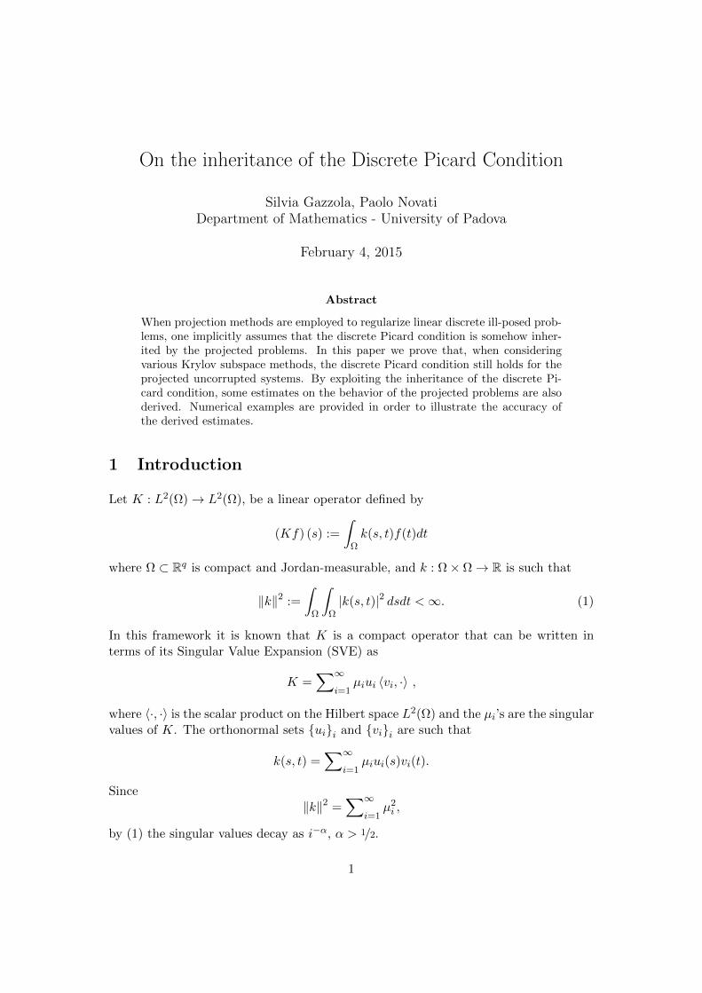
On the inheritance of the Discrete Picard Condition

Silvia Gazzola, Paolo NovatiDepartment of Mathematics - University of Padova

February 4, 2015

Abstract

When projection methods are employed to regularize linear discrete ill-posed prob-lems, one implicitly assumes that the discrete Picard condition is somehow inher-ited by the projected problems. In this paper we prove that, when consideringvarious Krylov subspace methods, the discrete Picard condition still holds for theprojected uncorrupted systems. By exploiting the inheritance of the discrete Pi-card condition, some estimates on the behavior of the projected problems are alsoderived. Numerical examples are provided in order to illustrate the accuracy ofthe derived estimates.

1 Introduction

Let K : L2(Ω)→ L2(Ω), be a linear operator defined by

(Kf) (s) :=

∫Ωk(s, t)f(t)dt

where Ω ⊂ Rq is compact and Jordan-measurable, and k : Ω× Ω→ R is such that

‖k‖2 :=

∫Ω

∫Ω|k(s, t)|2 dsdt <∞. (1)

In this framework it is known that K is a compact operator that can be written interms of its Singular Value Expansion (SVE) as

K =∑∞

i=1µiui 〈vi, ·〉 ,

where 〈·, ·〉 is the scalar product on the Hilbert space L2(Ω) and the µi’s are the singularvalues of K. The orthonormal sets uii and vii are such that

k(s, t) =∑∞

i=1µiui(s)vi(t).

Since‖k‖2 =

∑∞

i=1µ2i ,

by (1) the singular values decay as i−α, α > 1/2.

1

In this paper we consider the numerical solution of the linear equation

Kf = g, (2)

which is ill-posed in the sense of Hadamard (see [11, 14] for a background). The degreeof ill-posedness is characterized by the decay rate of the singular values. Equation (2)admits a solution f ∈ L2(Ω) if and only if the right-hand side g satisfies the so calledPicard Condition, that is,

∞∑i=1

(〈ui, g〉µi

)2

<∞, (3)

(cf., for instance, [5, §2.2]). Condition (3) implies that, as i → ∞, the absolute valueof the so-called Fourier coefficients 〈ui, g〉 decays to zero as i−αµi, α > 1/2.

After suitable discretization, depending on a parameter N , the solution of the linearequation (2) is approximated by the solution of a certain linear system (discrete ill-posedproblem)

A(N)x(N) = b(N), (4)

where the matrix A(N) inherits the spectral properties of K, and x(N) representsthe function f . Without loss of generality we may assume that A(N) ∈ RN×N ,b(N) ∈ RN . Let us consider the singular value decomposition (SVD) of A(N), givenby the factorization

A(N) = U (N)Σ(N)V (N)T , U (N) ∈ RN×N , Σ(N) ∈ RN×N , V (N) ∈ RN×N ,

where U (N)TU (N) = U (N)U (N)T = IN (i.e., the identity matrix of order N),

V (N)TV (N) = V (N)V (N)T = IN , and Σ(N) = diag(σ(N)1 , . . . , σ

(N)N ). We assume that,

independently of N , the σ(N)i ’s decay and cluster to zero with the same rate of the µi’s,

with no evident gap between two consecutive ones to indicate the numerical rank forA(N). If (2) is discretized by the Galerkin method, and N is sufficiently large, this isa meaningful assumption (see the analysis in [12]). Since the solution of (4) can bewritten as

x(N) =

N∑i=1

u(N)Ti b(N)

σ(N)i

vi,

in order to compute a meaningful solution of (4) the basic assumption is that thereexists a constant C such that

supN

N∑i=1

(u

(N)Ti b(N)

σ(N)i

)2

≤ C <∞, (5)

Alike the infinite dimensional problem (2), the above relation, which is called Discrete

Picard Condition (DPC, see [13]), implies that the Fourier coefficients |u(N)Ti b(N)| decay

to zero as i−ασ(N)i , α > 1/2, in order to ensure the convergence of the series. In this

situation, independently of N , we have

‖x(N)‖2 ≤ C <∞ .

2

In practice, when dealing with discrete models like (4), the DPC is not guaranteed to

hold since b(N) is usually affected by some error, i.e., b(N) = b(N)ex + e(N), where the

vector e(N) is assumed unknown. In the following, we always refer to the solution of

A(N)x(N) = b(N)ex as exact solution of (4). In particular, when e(N) is Gaussian white

noise, typically |u(N)Ti b(N)| decays until σ

(N)i > ‖e(N)‖2, and then stagnates around

‖e(N)‖2 (cf. [14, Chapter 4]). Still in [13], the author shows that the DPC plays animportant role in determining how well the Tikhonov or TSVD regularized solutionscan approximate the desired exact solution of (4). For this reason, when regularizingperturbed problems of the form (4), one usually assumes that the corresponding un-

perturbed problems satisfy the DPC, i.e., condition (5) applied to b(N)ex . Moreover, one

can devise a parameter choice strategy based on the so-called Picard plot (i.e., a plot of

the quantities |u(N)Ti b(N)| and σ

(N)i versus i, i = 1, . . . , N); the parameter selected by a

visual inspection of the Picard plot often agrees with the one selected by other popularparameter choice strategies (such as the L-curve and the GCV methods, cf. again thediscussion in [13]).

When dealing with large-scale problems, direct approaches to regularization (such asthe TSVD) are often unfeasible, because of their high computational cost; in these cases,just iterative or hybrid approaches to regularization are possible (cf. the discussion in[1]). Among the class of iterative regularization methods, a core role is played by Krylovsubspace methods, which allow to compute approximations of the solution of (4) bysolving projected subproblems of the form

W(N)Tk A(N)Z

(N)k y = W

(N)Tk b(N) or min

y

∥∥∥W (N)Tk+1 b(N) −W (N)T

k+1 A(N)Z(N)k y

∥∥∥ , (6)

where W(N)k and Z

(N)k are matrices whose columns span suitable Krylov subspaces of

dimension k. Here and in the following, ‖ · ‖ denotes the Euclidean vector norm. WhenKrylov subspace methods are employed to solve system (4) with a corrupted right-hand-side vector b(N), during the first iterations the approximate solutions typically converge

to the exact one (i.e., the solution of (4) with b(N) = b(N)ex ); then, as soon as the ap-

proximate solutions are affected by the high-frequency noise components perturbingb(N), they start to diverge. This behavior is known as semiconvergence phenomenon.Because of semiconvergence, a reliable stopping criterion is essential to perform iter-ative regularization. Alternatively, to overcome semiconvergence, one can resort tohybrid methods, in which the regularization of the projected problem is considered.Hybrid methods were originally introduced in [19] for the Lanczos-bidiagonalizationcase; hybrid methods based on the Arnoldi algorithm were cosidered in [4, 7].

During the last two decades, many Krylov subspace methods have been theoreticallyproved to be regularization methods in the classical sense, i.e., it has been provedthat the sequence of the approximate solutions tends to the exact solution of (4) when‖e(N)‖ → 0 and a suitable stopping criterion is considered (see for instance [10, Chap-ter 3] and [3]). More recently, the regularization and convergence properties of meth-ods based on the Arnoldi and the Lanczos bidiagonalization algorithms have beenanalyzed from the point of view of the spectral properties of the projected matrices

W(N)Tk A(N)Z

(N)k . In particular, the authors of [7, 18] experimentally show that the

3

behavior of the regularized solution obtained by truncating the Arnoldi process is sim-ilar to the one obtained by TSVD. Still in [7, 18], the rate of convergence of methodsbased on the Arnoldi algorithm is shown to be related to the decay rate of the singularvalues of A(N). Regarding hybrid methods, new parameter choice strategies have beendevised in [6, 16, 18] under the assumption that the original uncorrupted problem (4)satisfies the DPC. Finally, estimates on the behavior of the GMRES residual for theexact and the corrupted problems are given in [6] under the assumption that the DPCstill holds for the projected subproblems (6); this fact has been confirmed by manynumerical experiments performed on the most common test problems from [15].

From a theoretical point of view, the investigation of the inheritance of the DPC bythe projected subproblems (6) is still an open issue, which represents the goal of this

paper. Denoting by y(N)k the solution of (6), we say that the DPC is inherited if there

exists a constant C ′ such that

supk,N‖y(N)k ‖ ≤ C ′ <∞,

To establish the inheritance of the DPC when the exact (b(N) = b(N)ex ) problems (6)

are solved, we use a backward induction argument, i.e., we prove that if the (k + 1)thprojected problem satisfies the DPC, so does the kth one. Thanks to this result, we canderive further estimates on the behavior of the residuals associated to the projectionmethods (6), and we can give an alternative justification of the typical semiconvergent

behavior of the iterative methods applied to the corrupted (b(N) = b(N)ex +e(N)) problem

(4). Unless strictly necessary, from now on we avoid the use of the superscript (N),assuming it implicit by the context.

This paper is organized as follows: in Section 2 we provide a brief overview on theconsidered Krylov subspace methods, along with their hybrid versions. In Section 3,after giving some more details about the DPC, we prove that the DPC is inheritedwhen employing Arnoldi based methods (Section 3.1) and Lanczos bidiagonalizationbased methods (Section 3.2); we also analyze the behavior of the residuals for both theuncorrupted and the corrupted projected problems of the form (6). Our derivationsare supported by many numerical tests, whose most meaningful results are displayedalong Section 3. Finally, in Section 4 we present some concluding remarks.

Remarks about the numerical tests. All the considered test problems belong tothe package Regularization Tools [15]: in particular we display the results for the testproblems baart, wing (whose coefficient matrices are nonsymmetric), deriv2, and shaw

(whose coefficient matrices are symmetric); the coefficient matrix of the system (4) hassize 120 × 120 for all the test problems. All the computations have been performedusing Matlab 7.10 with 16 significant digits. Unless otherwise stated, we implement theArnoldi algorithm by Householder reflections [22, Chapter 6], and we implement theLanczos bidiagonalization algorithm with reorthogonalization following the indicationsin [21].

4

2 Regularization by Krylov Subspace Methods

Krylov subspaces methods are projection-type methods such that, at the kth iteration,an approximation xk of the solution of (4) is formed by imposing that

xk ∈ K(1)k and rk = b−Axk ⊥ K

(2)k , (7)

where K(i)k = Kk(Ci, di) = spandi, Cidi, . . . , Ck−1

i di, Ci ∈ RN×N , di ∈ RN ,i = 1, 2. Usually the matrices Ci and the vectors di depend on A and b. Formu-lation (7) intrinsically assumes that the initial guess x0 is the zero vector. Moreover,

in the following we always assume that dim(K(i)k ) = k, i = 1, 2.

2.1 The Arnoldi algorithm and the GMRES method

The Arnoldi algorithm [22, Chapter 6] underlies many of the most used Krylov methodsfor linear systems, and it is employed to compute an orthonormal basis for the spaceKk(A, b); more precisely, it leads to the decompositions

AWk = WkHk + hk+1,kwk+1eTk

= Wk+1Hk, (8)

where Wk+1 = [Wk wk+1] ∈ RN×(k+1) has orthonormal columns that span the Krylovsubspace Kk+1(A, b), ek is the kth element of the canonical basis of Rk (here and in thefollowing the dimension should be clear from the contest), and w1 = Wk+1e1 = b/ ‖b‖2.In the above relations, both Hk ∈ Rk×k and Hk ∈ R(k+1)×k are upper Hessenbergmatrices; Hk is obtained by discarding the last row of Hk. The Arnoldi algorithmterminates as soon as hk+1,k = 0, which means that an invariant subspace of A hasbeen computed.

Taking K(i)k = Kk(A, b), i = 1, 2 in (7), the Arnoldi algorithm can be used to construct

approximations of the solution of (4) in the following way (Full OrthogonalizationMethod, FOM)

xk = Wkyk, where yk = (Hk)−1ck , ck = ‖b‖e1 ∈ Rk. (9)

Besides FOM, the most highly-regarded Krylov subspace method based on the Arnoldialgorithm is the GMRES [22, Chapter 6], which is a projection method having

K(1)k = Kk(A, b) and K(2)

k = AKk(A, b). At the kth iteration, the GMRES prescribes totake as approximate solution of (4) the vector

xk = Wkyk, where yk = arg miny∈Rk

‖ ‖b‖e1︸ ︷︷ ︸ck∈Rk+1

−Hky‖. (10)

We note that the above projected problem is derived by taking into account relation(8). In the following, we employ the matrix relation

AWk = Wk+2H0k , where H0

k =

[Hk

0

]∈ R(k+2)×k, (11)

5

which is basically equivalent to (8). Indeed, the solution of the least squares problem

miny∈Rk

‖ ‖b‖e1︸ ︷︷ ︸ck+1∈Rk+2

−H0ky‖ , (12)

solves (10), and viceversa.

Hybrid methods formulated with respect to the Arnoldi algorithm and Tikhonov reg-ularization compute an approximate solution of the form xk,λ = Wkyk,λ, where

yk,λ = arg miny∈Rk

‖ck − Hky‖2 + λ2‖y‖2

; (13)

a suitable regularization parameter λ has to be set at each iteration (cf. [7]).

2.2 The Lanczos bidiagonalization algorithm and the LSQR method

The Lanczos (Golub-Kahan) bidiagonalization algorithm [8] is employed to computetwo matrices Wk, Zk ∈ RN×k having orthonormal columns, and being such thatR(Wk) = Kk(ATA,AT b) and R(Zk) = Kk(AAT , b). At the kth step, the Lanczosbidiagonalization algorithm can be expressed in matrix form by the following relations

ATZk = WkBTk ,

AWk = Zk+1Bk,

where both Bk ∈ Rk×k and Bk ∈ R(k+1)×k are lower bidiagonal; Bk is obtained bydeleting the last row of Bk; if we denote the diagonal elements of Bk by ζi, and itssub-diagonal elements by νi+1, i = 1, . . . , k, the Lanczos bidiagonalization algorithmterminates as soon as ζi = 0 or νi+1 = 0. The most highly-regarded Krylov subspacemethod based on the Lanczos bidiagonalization algorithm is the LSQR [21, 20], which

is a projection method having K(1)k = Kk(ATA,AT b) and K(2)

k = AKk(ATA,AT b). Atthe kth iteration, the LSQR prescribes to take as approximate solution of (4) the vector

xk = Wkyk, where yk = arg miny∈Rk

‖ ‖b‖e1︸ ︷︷ ︸ck∈Rk+1

−Bky‖ . (14)

Hybrid methods formulated with respect to the Lanczos bidiagonalization algorithmand Tikhonov regularization compute an approximate solution of the formxk,λ = Wkyk,λ, where

yk,λ = arg miny∈Rk

‖ck − Bky‖2 + λ2‖y‖2

; (15)

a suitable regularization parameter λ has to be set at each iteration (cf. [17] and thereferences therein).

6

3 Inheritance of the Discrete Picard Condition

As stated in the Introduction, the DPC holds for (4) if∣∣uTi b∣∣ = O(i−ασi

), α > 1/2, i→ N →∞.

In the following, we theoretically prove the inheritance of the DPC by backward induc-tion. We assume that both the Arnoldi and the Lanczos bidiagonalization algorithms donot break down until step N . This is not a restrictive assumption: indeed, if N∗ is thesmallest integer such that hN∗+1,N∗ = 0 (in the Arnoldi case), ζN∗ = 0 or νN∗+1 = 0 (inthe Lanczos bidiagonalization case), all the following derivations are still valid, providedthat N is replaced by N∗. We use the notation [z]i to denote the ith component of thevector z.

3.1 Methods based on the Arnoldi algorithm

Let us consider the SVD of the matrix H0k in (12), given by

H0k = U0

kΣkVTk , U0

k ∈ R(k+2)×k, Σk ∈ Rk×k, Vk ∈ Rk×k, (16)

where (U0k )TU0

k = Ik, (Vk)TVk = Vk(Vk)

T = Ik, and Σk = diag(σ(k)1 , . . . , σ

(k)k ). We

remark that the SVD of Hk is closely linked to (16): indeed,

Hk = UkΣkVTk , where Uk ∈ R(k+1)×k and U0

k =

[Uk0

]. (17)

In the following, we will extensively exploit an update formula for the SVD given in[2]. Since H0

k is obtained by deleting the last column of Hk+1, i.e.,

Hk+1 =[H0k , hk+1

]∈ R(k+2)×(k+1),

we can state thatU0k = Uk+1Xk+1, (18)

where Uk+1 is the matrix of the left singular values of Hk+1. The ith column x(k+1)i of

Xk+1 ∈ R(k+1)×k is computed by taking

x(k+1)i =

1∥∥∥∥(D(k+1)i

)−1w(k+1)

∥∥∥∥(D

(k+1)i

)−1w(k+1) ∈ Rk+1, i = 1, . . . , k , (19)

whereD

(k+1)i = (Σk+1)2 − (σ

(k)i )2Ik+1 ∈ R(k+1)×(k+1)

and Σk+1 is the diagonal matrix of the singular values of Hk+1. Therefore, D(k+1)i is

diagonal, and

w(k+1) =1

‖hk+1‖UTk+1hk+1 ∈ Rk+1 . (20)

7

Without loss of generality, in the following we assume that the component [w(k+1)]j ,

j = 1, . . . , k + 1, of w(k+1) (20) is different from zero, and that the σ(k+1)j ’s,

k = 1, . . . , N − 1, are distinct: this implies that the updated singular values σ(k)j ’s are

distinct. If this is not the case, then we have to perform deflation and we basically act onthe nonzero components of w(k+1) as we describe below

(see again [2] for the details). The singular values σ(k+1)j , j = 1, . . . , k + 1, and σ

(k)j ,

j = 1, . . . , k, are linked by the so-called (strict) interlacing property [9, §8.6.1]

σ(k+1)1 > σ

(k)1 > · · · > σ

(k+1)i > σ

(k)i > σ

(k+1)i+1 > · · · > σ

(k)k > σ

(k+1)k+1 . (21)

Since the singular values of HN and A obviously coincide (i.e., σ(N)j = σj), thanks to

(21) one has

σj − σ(k+1)j < σj − σ(k)

j ,

which shows that the convergence σ(k)j → σj for k → N is monotone. The next result

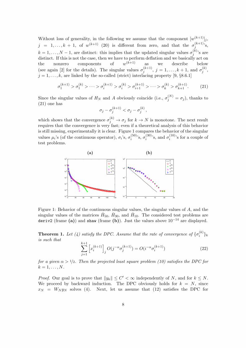
requires that the convergence is very fast; even if a theoretical analysis of this behavioris still missing, experimentally it is clear. Figure 1 compares the behavior of the singular

values µi’s (of the continuous operator), σi’s, σ(50)i ’s, σ

(30)i ’s, and σ

(10)i ’s for a couple of

test problems.

(a) (b)

0 20 40 60 80 100 12010

−6

10−5

10−4

10−3

10−2

10−1

100

µi

σi

σi

(50)

σi

(30)

σi

(10)

0 5 10 15 20 2510

−15

10−10

10−5

100

105

µi

σi

σi

(50)

σi

(30)

σi

(10)

Figure 1: Behavior of the continuous singular values, the singular values of A, and thesingular values of the matrices H50, H30, and H10. The considered test problems arederiv2 (frame (a)) and shaw (frame (b)). Just the values above 10−14 are displayed.

Theorem 1. Let (4) satisfy the DPC. Assume that the rate of convergence of σ(k)i k

is such thatk+1∑j=1

[x

(k+1)i

]jO(j−ασ

(k+1)j ) = O(i−ασ

(k+1)i ) (22)

for a given α > 1/2. Then the projected least square problem (10) satisfies the DPC fork = 1, . . . , N .

Proof. Our goal is to prove that ‖yk‖ ≤ C ′ < ∞ independently of N , and for k ≤ N .We proceed by backward induction. The DPC obviously holds for k = N , sincexN = WNyN solves (4). Next, let us assume that (12) satisfies the DPC for

8

2 ≤ k + 1 ≤ N , and let us prove that (12) satisfies the DPC for k. Thanks to re-lation (18), we can express the norm of the solution of (12) as

‖yk‖ = ‖(H0k)†ck+1‖

= ‖Σ−1k (U0

k )T ck+1‖=

∥∥Σ−1k XT

k+1UTk+1ck+1

∥∥Thanks to the DPC, there exists α > 1/2 such that∣∣∣[UTk+1ck+1

]j

∣∣∣ = O(j−ασ(k+1)j ) , j = 1, . . . , k + 1 ,

and hence

∣∣[Σ−1k XT

k+1UTk+1ck+1

]i

∣∣ =1

σ(k)i

k+1∑j=1

[x

(k+1)i

]j

[UTk+1ck+1

]j

= O(i−α) , i = 1, . . . , k ,

where we have exploited (22). This concludes the proof.

Remark 2. The hypothesis (22) substantially means that each row of XTk+1 is a dis-

cretization of the Delta function, or, in other words, that Xk+1 must be close to theidentity matrix. Despite this may appear as a very strong hypothesis, in practice we

can easily see that it is true thanks to the fast convergence of σ(k)i k. Indeed, defining

the quantities

ε(k+1)ij := (σ

(k+1)j )2 − (σ

(k)i )2, j = 1, . . . , k + 1, (23)

we can write

[x

(k+1)i

]2

i=

k+1∑j=1

[w(k+1)

]2j

ε(k+1)2ij

−1[w

(k+1)i

]2

i

ε(k+1)2ii

=

1 +ε

(k+1)2ii[w(k+1)

]2i

k+1∑j=1j 6=i

[w(k+1)

]2j

ε(k+1)2ij

−1

.

In this way,∣∣∣[x(k+1)

i ]i

∣∣∣ ' 1 provided that ε(k+1)ii /ε(k+1)

ij ' 0 for i 6= j, which is true if the

convergence of σ(k)i k is fast, and if σ

(k)i and σ

(k+1)j are well-separated for i 6= j. As a

clear consequence of ‖x(k+1)i ‖ = 1 (see (19)),

∣∣∣[x(k+1)i ]j

∣∣∣ ' 0 for i 6= j. This allows to

writex

(k+1)i = ei − δ(k+1)

i (24)

where

0 ≤ [δ(k+1)i ]i ≤

ε(k+1)2ii[w(k+1)

]2i

k+1∑j=1j 6=i

[w(k+1)

]2j

ε(k+1)2ij

(25)

9

andk+1∑j=1j 6=i

[δ

(k+1)i

]2

j≤ 2

[δ

(k+1)i

]i. (26)

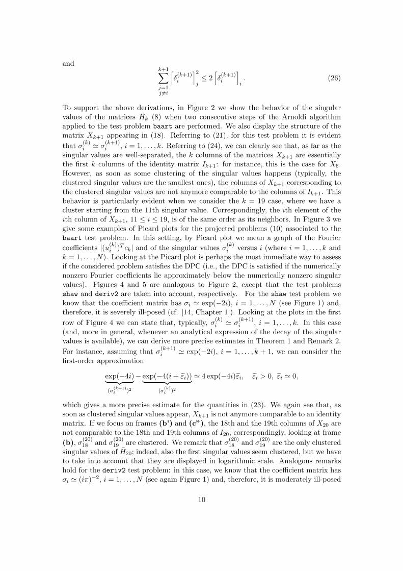
To support the above derivations, in Figure 2 we show the behavior of the singularvalues of the matrices Hk (8) when two consecutive steps of the Arnoldi algorithmapplied to the test problem baart are performed. We also display the structure of thematrix Xk+1 appearing in (18). Referring to (21), for this test problem it is evident

that σ(k)i ' σ(k+1)

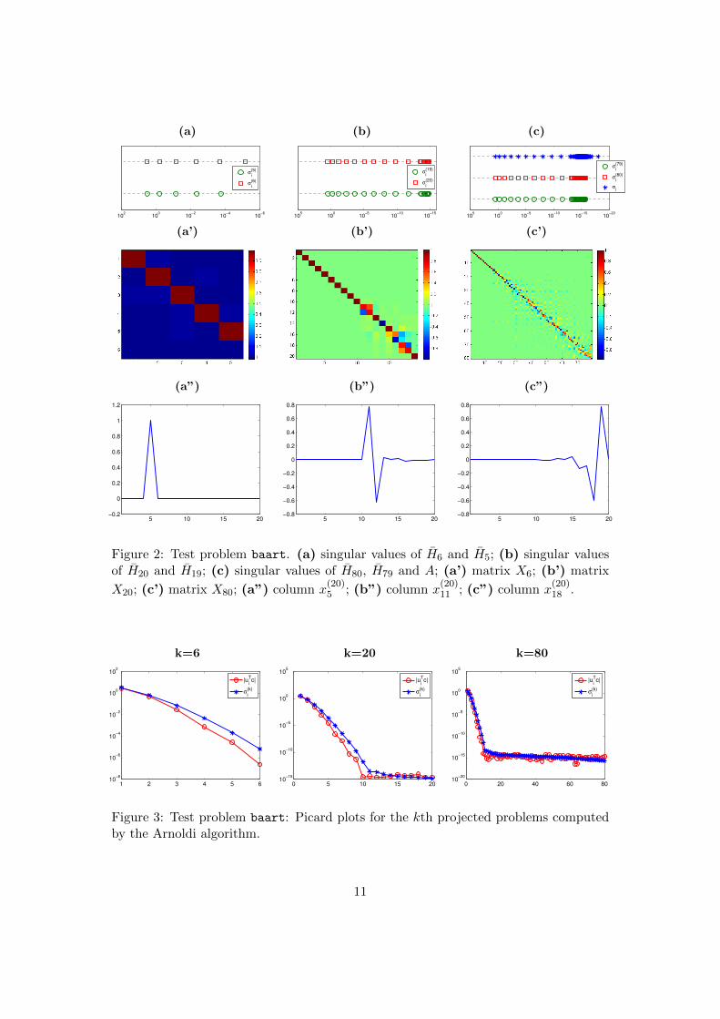
i , i = 1, . . . , k. Referring to (24), we can clearly see that, as far as thesingular values are well-separated, the k columns of the matrices Xk+1 are essentiallythe first k columns of the identity matrix Ik+1: for instance, this is the case for X6.However, as soon as some clustering of the singular values happens (typically, theclustered singular values are the smallest ones), the columns of Xk+1 corresponding tothe clustered singular values are not anymore comparable to the columns of Ik+1. Thisbehavior is particularly evident when we consider the k = 19 case, where we have acluster starting from the 11th singular value. Correspondingly, the ith element of theith column of Xk+1, 11 ≤ i ≤ 19, is of the same order as its neighbors. In Figure 3 wegive some examples of Picard plots for the projected problems (10) associated to thebaart test problem. In this setting, by Picard plot we mean a graph of the Fourier

coefficients |(u(k)i )T ck| and of the singular values σ

(k)i versus i (where i = 1, . . . , k and

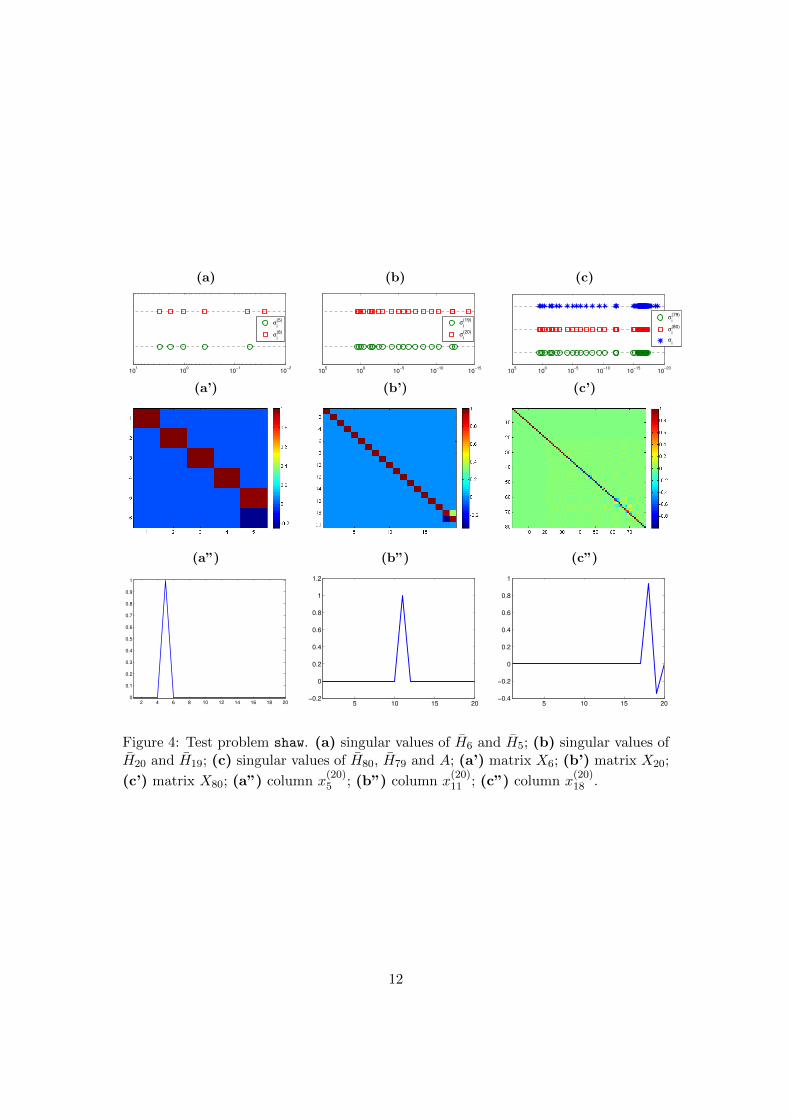
k = 1, . . . , N). Looking at the Picard plot is perhaps the most immediate way to assessif the considered problem satisfies the DPC (i.e., the DPC is satisfied if the numericallynonzero Fourier coefficients lie approximately below the numerically nonzero singularvalues). Figures 4 and 5 are analogous to Figure 2, except that the test problemsshaw and deriv2 are taken into account, respectively. For the shaw test problem weknow that the coefficient matrix has σi ' exp(−2i), i = 1, . . . , N (see Figure 1) and,therefore, it is severely ill-posed (cf. [14, Chapter 1]). Looking at the plots in the first

row of Figure 4 we can state that, typically, σ(k)i ' σ

(k+1)i , i = 1, . . . , k. In this case

(and, more in general, whenever an analytical expression of the decay of the singularvalues is available), we can derive more precise estimates in Theorem 1 and Remark 2.

For instance, assuming that σ(k+1)i ' exp(−2i), i = 1, . . . , k + 1, we can consider the

first-order approximation

exp(−4i)︸ ︷︷ ︸(σ

(k+1)i )2

− exp(−4(i+ εi))︸ ︷︷ ︸(σ

(k)i )2

' 4 exp(−4i)εi, εi > 0, εi ' 0,

which gives a more precise estimate for the quantities in (23). We again see that, assoon as clustered singular values appear, Xk+1 is not anymore comparable to an identitymatrix. If we focus on frames (b’) and (c”), the 18th and the 19th columns of X20 arenot comparable to the 18th and 19th columns of I20; correspondingly, looking at frame

(b), σ(20)18 and σ

(20)19 are clustered. We remark that σ

(20)18 and σ

(20)19 are the only clustered

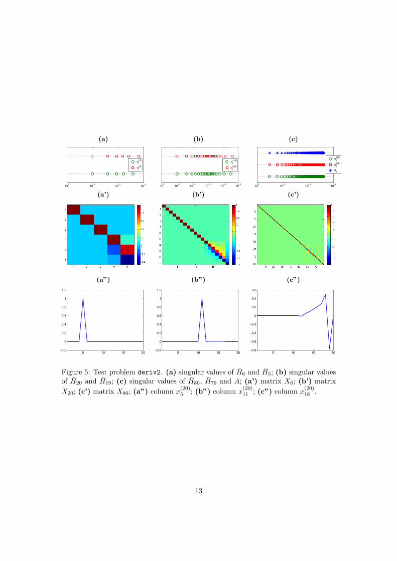
singular values of H20; indeed, also the first singular values seem clustered, but we haveto take into account that they are displayed in logarithmic scale. Analogous remarkshold for the deriv2 test problem: in this case, we know that the coefficient matrix hasσi ' (iπ)−2, i = 1, . . . , N (see again Figure 1) and, therefore, it is moderately ill-posed

10

(a) (b) (c)

10−6

10−4

10−2

100

102

σi

(5)

σi

(6)

10−15

10−10

10−5

100

105

σi

(19)

σi

(20)

10−20

10−15

10−10

10−5

100

105

σi

(79)

σi

(80)

σi

(a’) (b’) (c’)

(a”) (b”) (c”)

5 10 15 20−0.2

0

0.2

0.4

0.6

0.8

1

1.2

5 10 15 20−0.8

−0.6

−0.4

−0.2

0

0.2

0.4

0.6

0.8

5 10 15 20−0.8

−0.6

−0.4

−0.2

0

0.2

0.4

0.6

0.8

Figure 2: Test problem baart. (a) singular values of H6 and H5; (b) singular valuesof H20 and H19; (c) singular values of H80, H79 and A; (a’) matrix X6; (b’) matrix

X20; (c’) matrix X80; (a”) column x(20)5 ; (b”) column x

(20)11 ; (c”) column x

(20)18 .

k=6 k=20 k=80

1 2 3 4 5 610

−8

10−6

10−4

10−2

100

102

|ui

Tc|

σi

(k)

0 5 10 15 2010

−15

10−10

10−5

100

105

|ui

Tc|

σi

(k)

0 20 40 60 8010

−20

10−15

10−10

10−5

100

105

|ui

Tc|

σi

(k)

Figure 3: Test problem baart: Picard plots for the kth projected problems computedby the Arnoldi algorithm.

11

(a) (b) (c)

10−2

10−1

100

101

σi

(5)

σi

(6)

10−15

10−10

10−5

100

105

σi

(19)

σi

(20)

10−20

10−15

10−10

10−5

100

105

σi

(79)

σi

(80)

σi

(a’) (b’) (c’)

(a”) (b”) (c”)

2 4 6 8 10 12 14 16 18 20

0

0.1

0.2

0.3

0.4

0.5

0.6

0.7

0.8

0.9

1

5 10 15 20−0.2

0

0.2

0.4

0.6

0.8

1

1.2

5 10 15 20−0.4

−0.2

0

0.2

0.4

0.6

0.8

1

Figure 4: Test problem shaw. (a) singular values of H6 and H5; (b) singular values ofH20 and H19; (c) singular values of H80, H79 and A; (a’) matrix X6; (b’) matrix X20;

(c’) matrix X80; (a”) column x(20)5 ; (b”) column x

(20)11 ; (c”) column x

(20)18 .

12

(a) (b) (c)

10−3

10−2

10−1

100

σi

(5)

σi

(6)

10−5

10−4

10−3

10−2

10−1

100

σi

(19)

σi

(20)

10−6

10−4

10−2

100

σi

(79)

σi

(80)

σi

(a’) (b’) (c’)

(a”) (b”) (c”)

5 10 15 20−0.2

0

0.2

0.4

0.6

0.8

1

1.2

5 10 15 20−0.2

0

0.2

0.4

0.6

0.8

1

1.2

5 10 15 20−0.8

−0.6

−0.4

−0.2

0

0.2

0.4

0.6

Figure 5: Test problem deriv2. (a) singular values of H6 and H5; (b) singular valuesof H20 and H19; (c) singular values of H80, H79 and A; (a’) matrix X6; (b’) matrix

X20; (c’) matrix X80; (a”) column x(20)5 ; (b”) column x

(20)11 ; (c”) column x

(20)18 .

13

(cf. again [14, Chapter 1]). Looking at the plots in the first row of Figure 5, we can

still state that, typically, σ(k)i ' σ

(k+1)i , i = 1, . . . , k. Also in this case, assuming that

σ(k+1)i ' (iπ)−2, i = 1, . . . , k + 1, we can consider the first-order approximation

(iπ)−4︸ ︷︷ ︸(σ

(k+1)i )2

− ((i+ εi)π)−4︸ ︷︷ ︸(σ

(k)i )2

' 4

π4i−5εi, εi > 0, εi ' 0,

which is still analogous to (23).

In [6, Corollary 3], the authors give an estimate on the norm of the GMRES residualby assuming that the FOM inherits the DPC; more precisely, they prove that

‖rk‖ = O(k3/2σk) . (27)

In this setting we can rigorously prove that the FOM inherits the DPC by employingessentially the same arguments as Theorem 1. More precisely, in the transition fromthe (k + 1)th to the kth FOM iteration, we delete the (k + 1)th column of Hk+1 so toobtain Hk, and we delete the (k+ 1)th row of Hk so to obtain Hk. Just in this setting,we will denote the SVDs of the involved matrices in the following way:

Hk+1 = Uk+1Σk+1VTk+1, Hk = UkΣkV

Tk , Hk = UkΣkV

Tk .

To estimate the SVD of Hk, one should twice apply an update formula that is analogousto (18), and that is still derived in [2]. In particular: recalling that Hk = Hk+1[Ik , 0]T ,going from Hk+1 to Hk we get

Uk = Uk+1Xk+1 ;

recalling that Hk = [Ik , 0]Hk, going from Hk+1 to Hk we get

Uk = [Ik , 0]UkΣkXkΣ−1k .

At this point, the vector yk in (9) is such that

‖yk‖ =∥∥Σ−1

k UTk ck∥∥ =

∥∥∥∥∥∥∥∥∥Σ−2k XT

k ΣkUTk

[Ik0

]ck︸ ︷︷ ︸

ck+1

∥∥∥∥∥∥∥∥∥ =∥∥Σ−2

k XTk ΣkX

Tk+1U

Tk+1ck+1

∥∥ ,Let us assume that[

XTk z]j

= [z]j ∀z ∈ Rk, and[XTk+1

¯z]j

= [¯z]j ∀¯z ∈ Rk+1;

these assumptions are analogous to (22), and can be justified as in Remark 2. Since

there exists α > 1/2 such that∣∣∣[UTk+1ck+1

]j

∣∣∣ = O(j−ασ(k+1)j ), we get

∣∣∣[Σ−2k XT

k+1ΣkXTk+1U

Tk+1ck+1

]j

∣∣∣ =1

(σ(k)j )2

σ(k)j O(j−ασ

(k+1)j ) .

14

(a) (b)

10−20

10−15

10−10

10−5

100

105

σi

(20)

σi

(21)

10−15

10−10

10−5

100

105

σi

(20)

σi

(20)

(a’) (b’)

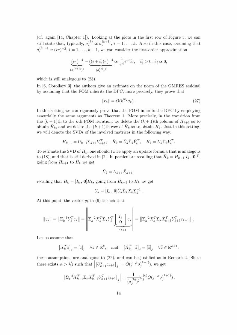
Figure 6: Test problem baart. (a) singular values of H21 and H20; (b) singular valuesof H20 and H20; (a’) matrix X21; (b’) matrix X20.

Thanks to the interlacing property of the singular values (which is twice applied: toHk+1 and Hk, and to Hk and Hk), we can conclude that ‖yk‖ < ∞. In Figure 6 wedisplay the interlacing property of the singular values, and the matrices Xk+1 and Xk

for k = 20 and the test problem baart.

Alternatively, under stricter assumptions, in the following proposition we give a newestimate on the norm of the GMRES residual without relying on the behavior of theFOM solution.

Proposition 3. Assume that (4) satisfies the DPC, and let rk = b − Axk be the kthresidual of GMRES applied to (4). Assume that the condition (24) holds. Then thereexists α > 1/2 such that

‖rk‖ = O(

(k + 1)−ασ(k+1)k+1

)+O

(∥∥∥δ(k+2)k+1

∥∥∥) (28)

where the components of δ(k+2)k+1 are analogous to (25), (26).

Proof. Thanks to relations (8) and (10),

rk = Wk+1

(ck − Hkyk

)= Wk+1

(Ik+1 − HkH

†k

)ck

= Wk+1

(Ik+1 − UkUTk

)ck, (29)

where Uk is the matrix appearing in (17). If we consider the complete SVD of Hk,given by

Hk = UkΣkVTk , Uk ∈ R(k+1)×(k+1), Σk+1 ∈ R(k+1)×k,

we have that Uk = [Uk , u(k)k+1]. Therefore, equality (29) can be rewritten as

rk = Wk+1u(k)k+1(u

(k)k+1)T ck. Thanks to the orthonormality of the columns of Wk+1

15

and u(k)k+1, we immediately get

‖rk‖ =∣∣∣(u(k)

k+1)T ck

∣∣∣ . (30)

Let us consider the reduced and complete SVDs of the matrices H0k (defined in (11))

and Hk+1, given by

H0k = U0

kΣkVTk = U0

k Σ0kV

Tk and Hk+1 = Uk+1Σk+1V

Tk+1 = Uk+1Σk+1V

Tk+1,

respectively. We remark that, in the above equalities,

U0k =

[Uk0

], U0

k = U0k

Ik00

, Uk+1 = Uk+1

[Ik+1

0

]. (31)

Analogously to (18), let us consider Xk+1 = UTk+1U0k ∈ R(k+1)×k, and

Xk+1 := UTk+1U0k ∈ R(k+2)×(k+2). We can immediately state that Xk+1 is orthogo-

nal and, directly from (31),

Xk+1 = [Ik+1 , 0] Xk+1

Ik00

.At this point, we can express u

(k)k+1 in the following way:

u(k)k+1 = [Ik+1 , 0] U0

kek+1 = [Ik+1 , 0] Uk+1Xk+1ek+1 = [Ik+1 , 0] Uk+1x(k+1)k+1 , (32)

where x(k+1)k+1 is the (k+ 1)th column of Xk+1. Thanks to (24) and the orthogonality of

Xk+1, we can write∣∣∣x(k+1)i

∣∣∣ = ei − δ(k+2)i ∈ Rk+2, for 1 ≤ i ≤ k + 1 , (33)

where the components of δ(k+2)i are defined as in (25) and (26). Directly from (30),

thanks to relations (32) and (33), the Cauchy-Schwarz inequality, and Theorem 1, wecan conclude that

‖rk‖ =∣∣∣(u(k)

k+1)T ck

∣∣∣ =

∣∣∣∣∣∣∣∣∣(x(k+1)k+1 )T UTk+1

[Ik0

]ck︸ ︷︷ ︸

ck+1

∣∣∣∣∣∣∣∣∣≤

∣∣∣eTk+1UTk+1ck+1

∣∣∣+∣∣∣(δ(k+2)

k+1 )T UTk+1ck+1

∣∣∣≤

∣∣∣(u(k+1)k+1 )T ck+1

∣∣∣+ ‖δ(k+2)k+1 ‖‖b‖

= O(

(k + 1)−ασ(k+1)k+1

)+O

(∥∥∥δ(k+2)i

∥∥∥) , α > 1/2 ,

where u(k+1)k+1 is the (k + 1)th column of Uk+1.

16

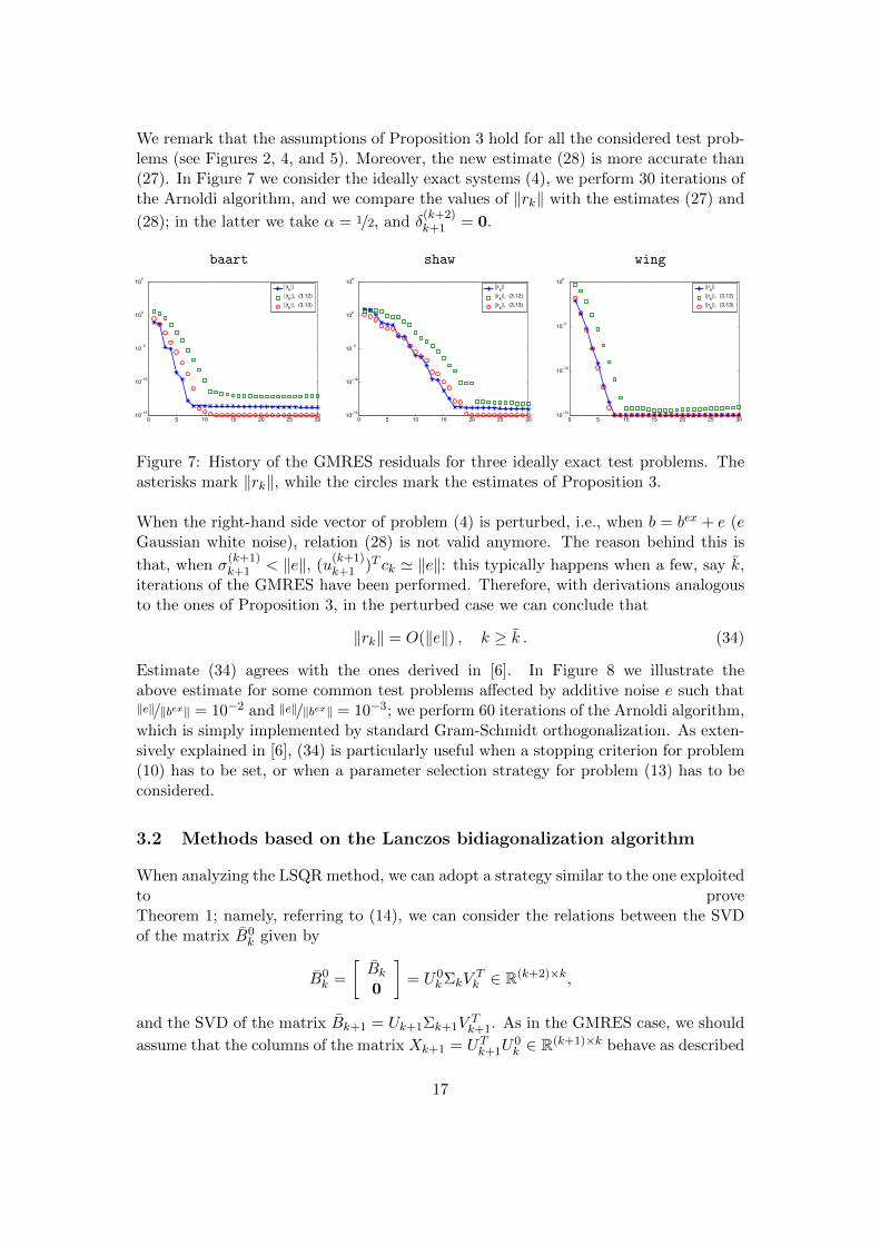
We remark that the assumptions of Proposition 3 hold for all the considered test prob-lems (see Figures 2, 4, and 5). Moreover, the new estimate (28) is more accurate than(27). In Figure 7 we consider the ideally exact systems (4), we perform 30 iterations ofthe Arnoldi algorithm, and we compare the values of ‖rk‖ with the estimates (27) and

(28); in the latter we take α = 1/2, and δ(k+2)k+1 = 0.

baart shaw wing

0 5 10 15 20 25 3010

−15

10−10

10−5

100

105

||rk||

||rk||, (3.12)

||rk||, (3.13)

0 5 10 15 20 25 3010

−15

10−10

10−5

100

105

||rk||

||rk||, (3.12)

||rk||, (3.13)

0 5 10 15 20 25 3010

−15

10−10

10−5

100

||rk||

||rk||, (3.12)

||rk||, (3.13)

Figure 7: History of the GMRES residuals for three ideally exact test problems. Theasterisks mark ‖rk‖, while the circles mark the estimates of Proposition 3.

When the right-hand side vector of problem (4) is perturbed, i.e., when b = bex + e (eGaussian white noise), relation (28) is not valid anymore. The reason behind this is

that, when σ(k+1)k+1 < ‖e‖, (u

(k+1)k+1 )T ck ' ‖e‖: this typically happens when a few, say k,

iterations of the GMRES have been performed. Therefore, with derivations analogousto the ones of Proposition 3, in the perturbed case we can conclude that

‖rk‖ = O(‖e‖) , k ≥ k . (34)

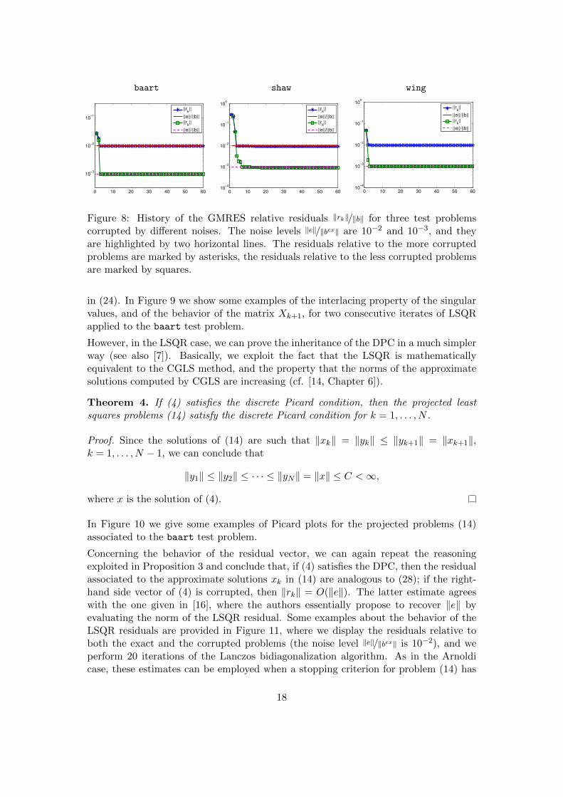
Estimate (34) agrees with the ones derived in [6]. In Figure 8 we illustrate theabove estimate for some common test problems affected by additive noise e such that‖e‖/‖bex‖ = 10−2 and ‖e‖/‖bex‖ = 10−3; we perform 60 iterations of the Arnoldi algorithm,which is simply implemented by standard Gram-Schmidt orthogonalization. As exten-sively explained in [6], (34) is particularly useful when a stopping criterion for problem(10) has to be set, or when a parameter selection strategy for problem (13) has to beconsidered.

3.2 Methods based on the Lanczos bidiagonalization algorithm

When analyzing the LSQR method, we can adopt a strategy similar to the one exploitedto proveTheorem 1; namely, referring to (14), we can consider the relations between the SVDof the matrix B0

k given by

B0k =

[Bk0

]= U0

kΣkVTk ∈ R(k+2)×k,

and the SVD of the matrix Bk+1 = Uk+1Σk+1VTk+1. As in the GMRES case, we should

assume that the columns of the matrix Xk+1 = UTk+1U0k ∈ R(k+1)×k behave as described

17

baart shaw wing

0 10 20 30 40 50 60

10−3

10−2

10−1

||rk||

||e||/||b||

||rk||

||e||/||b||

0 10 20 30 40 50 6010

−4

10−3

10−2

10−1

100

||rk||

||e||/||b||

||rk||

||e||/||b||

0 10 20 30 40 50 6010

−4

10−3

10−2

10−1

100

||rk||

||e||/||b||

||rk||

||e||/||b||

Figure 8: History of the GMRES relative residuals ‖rk‖/‖b‖ for three test problemscorrupted by different noises. The noise levels ‖e‖/‖bex‖ are 10−2 and 10−3, and theyare highlighted by two horizontal lines. The residuals relative to the more corruptedproblems are marked by asterisks, the residuals relative to the less corrupted problemsare marked by squares.

in (24). In Figure 9 we show some examples of the interlacing property of the singularvalues, and of the behavior of the matrix Xk+1, for two consecutive iterates of LSQRapplied to the baart test problem.

However, in the LSQR case, we can prove the inheritance of the DPC in a much simplerway (see also [7]). Basically, we exploit the fact that the LSQR is mathematicallyequivalent to the CGLS method, and the property that the norms of the approximatesolutions computed by CGLS are increasing (cf. [14, Chapter 6]).

Theorem 4. If (4) satisfies the discrete Picard condition, then the projected leastsquares problems (14) satisfy the discrete Picard condition for k = 1, . . . , N .

Proof. Since the solutions of (14) are such that ‖xk‖ = ‖yk‖ ≤ ‖yk+1‖ = ‖xk+1‖,k = 1, . . . , N − 1, we can conclude that

‖y1‖ ≤ ‖y2‖ ≤ · · · ≤ ‖yN‖ = ‖x‖ ≤ C <∞,

where x is the solution of (4).

In Figure 10 we give some examples of Picard plots for the projected problems (14)associated to the baart test problem.

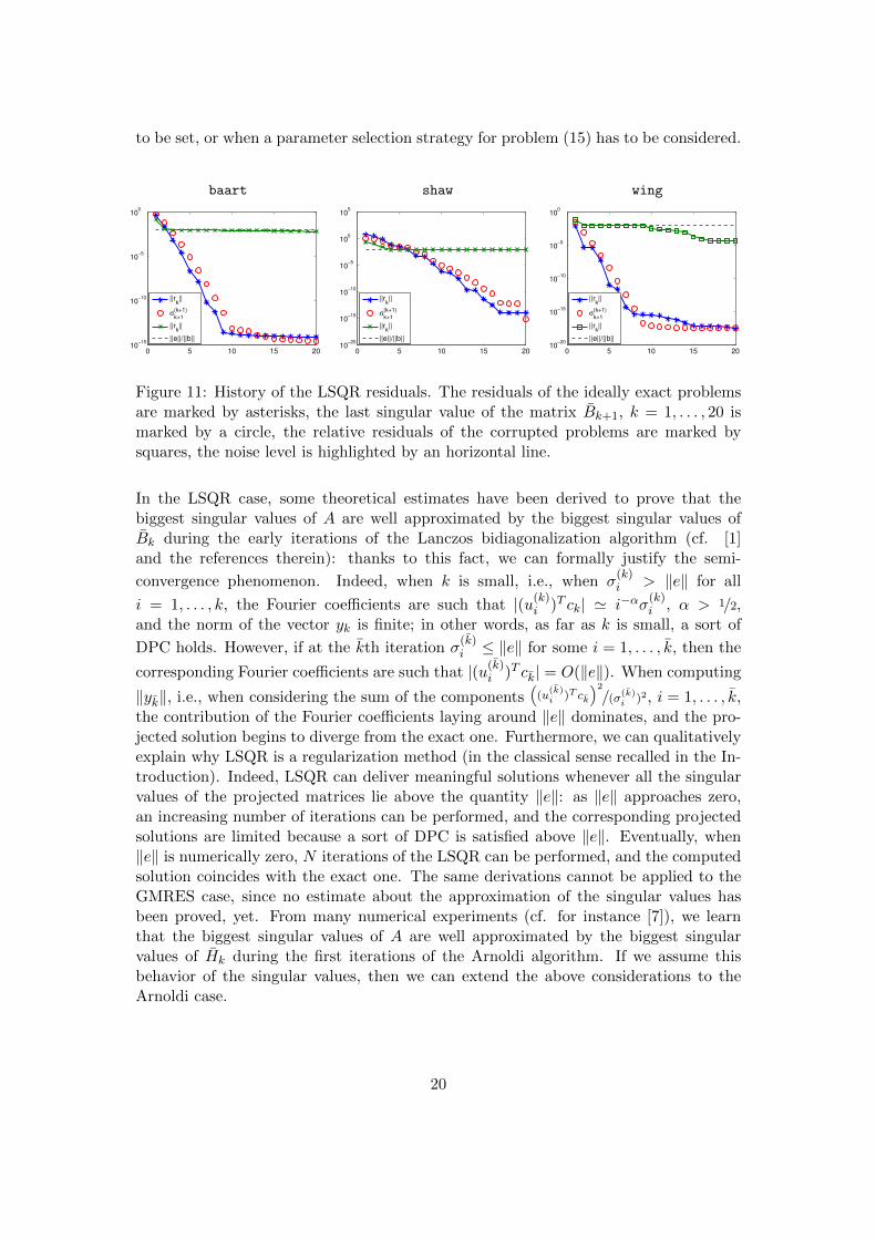
Concerning the behavior of the residual vector, we can again repeat the reasoningexploited in Proposition 3 and conclude that, if (4) satisfies the DPC, then the residualassociated to the approximate solutions xk in (14) are analogous to (28); if the right-hand side vector of (4) is corrupted, then ‖rk‖ = O(‖e‖). The latter estimate agreeswith the one given in [16], where the authors essentially propose to recover ‖e‖ byevaluating the norm of the LSQR residual. Some examples about the behavior of theLSQR residuals are provided in Figure 11, where we display the residuals relative toboth the exact and the corrupted problems (the noise level ‖e‖/‖bex‖ is 10−2), and weperform 20 iterations of the Lanczos bidiagonalization algorithm. As in the Arnoldicase, these estimates can be employed when a stopping criterion for problem (14) has

18

(a) (b) (c)

10−6

10−4

10−2

100

102

σi

(5)

σi

(6)

10−15

10−10

10−5

100

105

σi

(19)

σi

(20)

10−20

10−10

100

1010

σi

(79)

σi

(80)

σi

(a’) (b’) (c’)

(a”) (b”) (c”)

5 10 15 20−0.2

0

0.2

0.4

0.6

0.8

1

1.2

5 10 15 20−0.2

0

0.2

0.4

0.6

0.8

1

1.2

5 10 15 20−0.8

−0.6

−0.4

−0.2

0

0.2

0.4

0.6

Figure 9: Test problem baart. (a) singular values of B6 and B5; (b) singular values ofB20 and B19; (c) singular values of B80, B79 and A; (a’) matrix X6; (b’) matrix X20;

(c’) matrix X80;(a”) column x(20)5 ; (b”) column x

(20)11 ; (c”) column x

(20)18 .

k=6 k=20 k=80

1 2 3 4 5 610

−8

10−6

10−4

10−2

100

102

|ui

Tc|

σi

(k)

0 5 10 15 2010

−20

10−15

10−10

10−5

100

105

|ui

Tc|

σi

(k)

0 20 40 60 8010

−20

10−15

10−10

10−5

100

105

|ui

Tc|

σi

(k)

Figure 10: Test problem baart: Picard plots for the kth projected problems computedby the Lanczos bidiagonalization algorithm.

19

to be set, or when a parameter selection strategy for problem (15) has to be considered.

baart shaw wing

0 5 10 15 2010

−15

10−10

10−5

100

||rk||

σk+1

(k+1)

||rk||

||e||/||b||

0 5 10 15 2010

−20

10−15

10−10

10−5

100

105

||rk||

σk+1

(k+1)

||rk||

||e||/||b||

0 5 10 15 2010

−20

10−15

10−10

10−5

100

||rk||

σk+1

(k+1)

||rk||

||e||/||b||

Figure 11: History of the LSQR residuals. The residuals of the ideally exact problemsare marked by asterisks, the last singular value of the matrix Bk+1, k = 1, . . . , 20 ismarked by a circle, the relative residuals of the corrupted problems are marked bysquares, the noise level is highlighted by an horizontal line.

In the LSQR case, some theoretical estimates have been derived to prove that thebiggest singular values of A are well approximated by the biggest singular values ofBk during the early iterations of the Lanczos bidiagonalization algorithm (cf. [1]and the references therein): thanks to this fact, we can formally justify the semi-

convergence phenomenon. Indeed, when k is small, i.e., when σ(k)i > ‖e‖ for all

i = 1, . . . , k, the Fourier coefficients are such that |(u(k)i )T ck| ' i−ασ

(k)i , α > 1/2,

and the norm of the vector yk is finite; in other words, as far as k is small, a sort of

DPC holds. However, if at the kth iteration σ(k)i ≤ ‖e‖ for some i = 1, . . . , k, then the

corresponding Fourier coefficients are such that |(u(k)i )T ck| = O(‖e‖). When computing

‖yk‖, i.e., when considering the sum of the components(

(u(k)i )T ck

)2

/(σ(k)i )2, i = 1, . . . , k,

the contribution of the Fourier coefficients laying around ‖e‖ dominates, and the pro-jected solution begins to diverge from the exact one. Furthermore, we can qualitativelyexplain why LSQR is a regularization method (in the classical sense recalled in the In-troduction). Indeed, LSQR can deliver meaningful solutions whenever all the singularvalues of the projected matrices lie above the quantity ‖e‖: as ‖e‖ approaches zero,an increasing number of iterations can be performed, and the corresponding projectedsolutions are limited because a sort of DPC is satisfied above ‖e‖. Eventually, when‖e‖ is numerically zero, N iterations of the LSQR can be performed, and the computedsolution coincides with the exact one. The same derivations cannot be applied to theGMRES case, since no estimate about the approximation of the singular values hasbeen proved, yet. From many numerical experiments (cf. for instance [7]), we learnthat the biggest singular values of A are well approximated by the biggest singularvalues of Hk during the first iterations of the Arnoldi algorithm. If we assume thisbehavior of the singular values, then we can extend the above considerations to theArnoldi case.

20

4 Conclusions

In this paper we proved that the DPC is inherited when the GMRES and the LSQRmethods are employed to solve linear problems satisfying the DPC: to do this weexploited some general SVD update formulas. For this reason we believe that the samereasoning can be applied to other Krylov subspace methods based on the Arnoldi andLanczos bidiagonalization algorithms (including their range-restricted variants), andcan be extended to other generic projection methods (for instance, the ones based onthe nonsymmetric Lanczos algorithm, [22, Chapter 7]). Starting from the inheritanceof the DPC, other properties of the GMRES and LSQR methods have been recovered:more precisely, we revisited some estimates on the behavior of the residuals, and we gavea further justification of the semiconvergence phenomenon. We believe that, thanksto the inheritance of the DPC, similar properties can be proved for a wider class ofprojection methods.

References

[1] S. Berisha and J. G. Nagy. Iterative image restoration. In R. Chellappa andS. Theodoridis, editors, Academic Press Library in Signal Processing, volume 4,chapter 7, pages 193–243. Elsevier, 2014.

[2] J. R. Bunch and C. P. Nielsen. Upadating the Singular Value Decomposition.Numer. Math., 31:111–129, 1978.

[3] D. Calvetti, B. Lewis, and L. Reichel. On the regularizing properties of the GMRESmethod. Numer. Math., 91:605–625, 2002.

[4] D. Calvetti, S. Morigi, L. Reichel, and F. Sgallari. Tikhonov regularization and theL-curve for large discrete ill-posed problems. J. Comput. Appl. Math., 123:423–446,2000.

[5] H. W. Engl, M. Hanke, and A. Neubauer. Regularization of Inverse Problems.Kluwer Academic Publishers, Dordrecht, 2000.

[6] S. Gazzola, P. Novati, and M. R. Russo. Embedded techniques for choosing theparameter in Tikhonov regularization. Numer. Linear Algebra Appl., 21(6):796–812, 2014.

[7] S. Gazzola, P. Novati, and M. R. Russo. On Krylov projection methods andTikhonov regularization. Electron. Trans. Numer. Anal., 2015. To Appear.

[8] G. H. Golub and W. Kahan. Calculating the singular values and pseudo-inverseof a matrix. SIAM J. Numer. Anal., 2:205–224, 1965.

[9] G. H. Golub and C. F. Van Loan. Matrix Computations. The Johns HopkinsUniversity Press, Baltimore, MD, third edition, 1996.

[10] M. Hanke. Conjugate Gradient Type Methods for Ill-Posed Problems. Longman,Essex, UK, 1995.

21

[11] M. Hanke and P. C. Hansen. Regularization methods for large-scale problems.Surv. Math. Ind., 3:253–315, 1993.

[12] P. C. Hansen. Computation of the singular value expansion. Computing, 40(3):185–199, 1988.

[13] P. C. Hansen. The discrete Picard condition for discrete ill-posed problems. BIT,30:658–672, 1990.

[14] P. C. Hansen. Rank-deficient and discrete ill-posed problems. SIAM, Philadelphia,PA, 1998.

[15] P. C. Hansen. Regularization Tools: A Matlab package for analysis and solutionof discrete ill-posed problems, 2008.http://www2.imm.dtu.dk/~pcha/Regutools/RTv4manual.pdf.

[16] I. Hnetynkova, M. Plesinger, and Z. Strakos. The regularizing effect of the Golub-Kahan iterative bidiagonalization and revealing the noise level in the data. BIT,49:669–696, 2009.

[17] M. E. Kilmer and D.P. O’Leary. Choosing regularization parameters in iterativemethods for ill-posed problems. SIAM J. Matrix Anal. Appl., 22(4):1204–1221,2001.

[18] P. Novati and M. R. Russo. A GCV based Arnoldi-Tikhonov regularizationmethod. BIT, 54(2):501–521, 2014.

[19] D. P. O’Leary and J. A. Simmons. A bidiagonalization-regularization procedurefor large scale discretizations of ill-posed problems. SIAM J. Sci. Stat. Comp.,2(4):474–489, 1981.

[20] C. C. Paige and M. A. Saunders. Algorithm 583 LSQR: sparse linear equationsand sparse least squares. ACM Trans. Math. Software, 8:195–209, 1982.

[21] C. C. Paige and M. A. Saunders. LSQR: an algorithm for sparse linear equationsand and sparse least squares. ACM Trans. Math. Software, 8:43–71, 1982.

[22] Y. Saad. Iterative Methods for Sparse Linear Systems, 2nd Ed. SIAM, Philadel-phia, PA, 2003.

22