Embed Size (px)
Citation preview

1
On the Inconsistency between CAPM and the Utility Theory
Jing Chen School of Business University of Northern British Columbia Prince George, BC Canada V2N 4Z9 Phone: 1-250-960-6480 Email: [email protected] Web: http://web.unbc.ca/~chenj/
This version: February, 2019 Abstract
CAPM assumes investors maximize their utility. We construct a simple asset world with one risk free asset and two risky assets. We derive the expected return and variance of each asset with log utility function. The results are different from CAPM. Specifically, the expected return of asset with low (high) beta is higher (lower) than predicted by CAPM. The results obtained from the utility theory is more consistent with empirical data than CAPM. All the calculations and tables in this paper are contained in an Excel file, which can be downloaded at http://web.unbc.ca/~chenj/papers/CAPM.xlsx

2
1. Introduction
Capital asset pricing model (CAPM) was developed more than half century ago (Sharpe, 1964;
Lintner, 1965). It has since become the foundation of investment theory. CAPM is an important
tool in investment and corporate finance. CAPM, in its original form, is very elegant. However,
CAPM fits empirical data poorly (Fama and French, 2004). Many elaborate modifications of
CAPM have been proposed. With increasing complexity of these modifications, it is time to
reexamine the theoretical foundation of CAPM.
Return distribution of assets is ultimately determined by the trading decisions of the investors.
People trade to maximize expected gains under uncertainty, which are measured by utility
functions. In developing CAPM, Sharpe (1964) assumed investors maximizing their utility. He
made extensive discussion on how investor preference affect return distribution of assets. But in
formulating the quantitative theory of CAPM in the final section of his paper, he did not make use
of investor utility. Indeed, he didn’t need investor preference in formulating CAPM.
In reality, investor preferences affect asset pricing (Mehra and Prescott, 1985). We will directly
examine how asset allocation decisions by investors affect asset prices when investors maximize
their utility function. We construct a simple market with two risky assets and one risk free asset.
The distributions of the final payoffs of the two risky assets are given. The investors are assumed
to maximize logarithmic utility function. We apply the method of Lagrange multipliers to obtain
the prices of different assets. With asset prices, the expected rates of return and variances can be

3
calculated. We showed that, utility theory, by itself, can determine expected rate of returns and
variances of assets.
In effect, CAPM and utility theory are two asset pricing theories that can determine the return
distributions of assets. Do two models provide the same theoretical predictions? We show that
the results from utility theory differ from that from CAPM. Specifically, the expected return of
the asset with small (large) beta calculated from the utility theory is higher (lower) than that from
CAPM, and the expected return of the asset of small (large) size is higher (lower) than that from
CAPM. These theoretical calculations from utility theory are more consistent with empirical data
(Black, Jensen and Scholes, 1972; Fama and French, 1993).
On the technical level, we show that the method of Lagrange multipliers, when applied to utility
theory, can yield a great amount of information on asset pricing. For example, we can explicitly
calculate how the amount of supply of one asset affects the pricing of all assets quantitatively. The
results are consistent with intuition. Many detailed properties about the return distributions of the
assets can be derived from the utility theory. These properties can be tested empirically.
The results obtained in this paper can be understood from another perspective. In Figure 6 of
Sharpe (1964), many, instead of single, portfolios lie on the capital market line. In Note 18 of the
paper, Sharpe further stated,

4
“The area in Figure 6 representing ER and σR values attained with only risky assets has been
drawn at some distance from the horizontal axis for emphasis. It is likely that a more
accurate representation would place it very close to the axis.” (Sharpe, 1964, p. 435)
Short term debt markets are very liquid. The short term debt instruments, and hence the risky
assets, form a continuous spectrum to the risk free asset (Chen, 2010). When the efficient frontier
of the risky assets form a continuous spectrum to the risky free asset, as it is the case in the actual
market, the derivation of CAPM model presented in the last section of Sharpe is no more valid.
Hence we should not expect it to provide good approximation to the market data.

5
2. The Derivation of main results
In a simple market, there are three assets. One is risk free asset. The other two assets are risky
asset. The risk free asset provides a payoff of B at the end of one unit of time. The first risky asset,
S, has two potential payoffs, S1, S2, each with probability 50%. The second risky asset, T, has two
potential payoffs, T1, T2, each with probability 50%. We further assume the payoffs of S and T are
independent. Together, there are four potential payoff outcomes, (S1, T1), (S1, T2), (S2, T1), (S2,
T2), each with a probability of 25%. Suppose the prices of B, S and T are m, x and y. The goal of
an investor is to maximize his expected geometric average of the investment value at the end of
the time period. Equivalently, he attempts to maximize the lognormal utility of his wealth.
Without loss of generality, we assume the investor has one dollar to invest. The amounts the
investor will invest in B, S and T are P0, P1 and P2 respectively.
P0+P1+P2 = 1
When the final values of S and T are S1 and T1, the final portfolio value of the investor will be
𝑃𝑃0𝐵𝐵𝑚𝑚
+ 𝑃𝑃1𝑆𝑆1𝑥𝑥
+ 𝑃𝑃2𝑇𝑇1𝑦𝑦
When the final values of S and T are S1 and T2, the final portfolio value of the investor will be
𝑃𝑃0𝐵𝐵𝑚𝑚
+ 𝑃𝑃1𝑆𝑆1𝑥𝑥
+ 𝑃𝑃2𝑇𝑇2𝑦𝑦
When the final values of S and T are S2 and T1, the final portfolio value of the investor will be
𝑃𝑃0𝐵𝐵𝑚𝑚
+ 𝑃𝑃1𝑆𝑆2𝑥𝑥
+ 𝑃𝑃2𝑇𝑇1𝑦𝑦
When the final values of S and T are S2 and T2, the final portfolio value of the investor will be

6
𝑃𝑃0𝐵𝐵𝑚𝑚
+ 𝑃𝑃1𝑆𝑆2𝑥𝑥
+ 𝑃𝑃2𝑇𝑇2𝑦𝑦
Since we will use above four functions repeatedly, we give them shorter symbols 1’ , 2’ , 3’ , and 4’
to represent them. The goal of the investor is to maximize the geometric mean of his wealth, or
{(𝑃𝑃0𝐵𝐵𝑚𝑚
+ 𝑃𝑃1𝑆𝑆1𝑥𝑥
+ 𝑃𝑃2𝑇𝑇1𝑦𝑦
)(𝑃𝑃0𝐵𝐵𝑚𝑚
+ 𝑃𝑃1𝑆𝑆1𝑥𝑥
+ 𝑃𝑃2𝑇𝑇2𝑦𝑦
)(𝑃𝑃0𝐵𝐵𝑚𝑚
+ 𝑃𝑃1𝑆𝑆2𝑥𝑥
+ 𝑃𝑃2𝑇𝑇1𝑦𝑦
)(𝑃𝑃0𝐵𝐵𝑚𝑚
+ 𝑃𝑃1𝑆𝑆2𝑥𝑥
+ 𝑃𝑃2𝑇𝑇2𝑦𝑦
)}14
To simplify the calculation, we will attempt to maximize the equivalent form by removing the ¼
power in the above expression,
(𝑃𝑃0𝐵𝐵𝑚𝑚
+ 𝑃𝑃1𝑆𝑆1𝑥𝑥
+ 𝑃𝑃2𝑇𝑇1𝑦𝑦
) �𝑃𝑃0𝐵𝐵𝑚𝑚
+ 𝑃𝑃1𝑆𝑆1𝑥𝑥
+ 𝑃𝑃2𝑇𝑇2𝑦𝑦� �𝑃𝑃0
𝐵𝐵𝑚𝑚
+ 𝑃𝑃1𝑆𝑆2𝑥𝑥
+ 𝑃𝑃2𝑇𝑇1𝑦𝑦� �𝑃𝑃0
𝐵𝐵𝑚𝑚
+ 𝑃𝑃1𝑆𝑆2𝑥𝑥
+ 𝑃𝑃2𝑇𝑇2𝑦𝑦� (1)
Or a shorter form
1’ * 2’ *3’ *4’
where
1’ = 𝑃𝑃0𝐵𝐵𝑚𝑚
+ 𝑃𝑃1𝑆𝑆1𝑥𝑥
+ 𝑃𝑃2𝑇𝑇1𝑦𝑦
(2)
2’ = 𝑃𝑃0𝐵𝐵𝑚𝑚
+ 𝑃𝑃1𝑆𝑆1𝑥𝑥
+ 𝑃𝑃2𝑇𝑇2𝑦𝑦
(3)
3’ = 𝑃𝑃0𝐵𝐵𝑚𝑚
+ 𝑃𝑃1𝑆𝑆2𝑥𝑥
+ 𝑃𝑃2𝑇𝑇1𝑦𝑦
(4)
7
4′ = 𝑃𝑃0𝐵𝐵𝑚𝑚
+ 𝑃𝑃1𝑆𝑆2𝑥𝑥
+ 𝑃𝑃2𝑇𝑇2𝑦𝑦
(5)
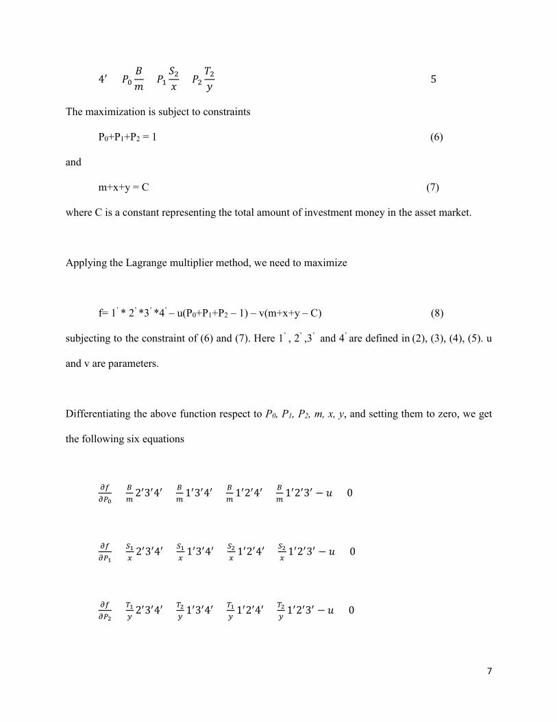
The maximization is subject to constraints
P0+P1+P2 = 1 (6)
and
m+x+y = C (7)
where C is a constant representing the total amount of investment money in the asset market.
Applying the Lagrange multiplier method, we need to maximize
f= 1’ * 2’ *3’ *4’ – u(P0+P1+P2 – 1) – v(m+x+y – C) (8)
subjecting to the constraint of (6) and (7). Here 1’ , 2’ ,3’ and 4’ are defined in (2), (3), (4), (5). u
and v are parameters.
Differentiating the above function respect to P0, P1, P2, m, x, y, and setting them to zero, we get
the following six equations
𝜕𝜕𝜕𝜕𝜕𝜕𝑃𝑃0
= 𝐵𝐵𝑚𝑚
2′3′4′ + 𝐵𝐵𝑚𝑚
1′3′4′ + 𝐵𝐵𝑚𝑚
1′2′4′ + 𝐵𝐵𝑚𝑚
1′2′3′ − 𝑢𝑢 = 0
𝜕𝜕𝜕𝜕𝜕𝜕𝑃𝑃1
= 𝑆𝑆1𝑥𝑥
2′3′4′ + 𝑆𝑆1𝑥𝑥
1′3′4′ + 𝑆𝑆2𝑥𝑥
1′2′4′ + 𝑆𝑆2𝑥𝑥
1′2′3′ − 𝑢𝑢 = 0
𝜕𝜕𝜕𝜕𝜕𝜕𝑃𝑃2
= 𝑇𝑇1𝑦𝑦
2′3′4′ + 𝑇𝑇2𝑦𝑦
1′3′4′ + 𝑇𝑇1𝑦𝑦
1′2′4′ + 𝑇𝑇2𝑦𝑦
1′2′3′ − 𝑢𝑢 = 0

8
𝜕𝜕𝜕𝜕𝜕𝜕𝑚𝑚
= −𝑃𝑃0𝐵𝐵𝑚𝑚2 2′3′4′ − 𝑃𝑃0𝐵𝐵
𝑚𝑚2 1′3′4′ − 𝑃𝑃0𝐵𝐵𝑚𝑚2 1′2′4′ − 𝑃𝑃0𝐵𝐵
𝑚𝑚2 1′2′3′ − 𝑣𝑣 = 0
𝜕𝜕𝜕𝜕𝜕𝜕𝑥𝑥
= −𝑃𝑃1𝑆𝑆1𝑥𝑥2
2′3′4′ − 𝑃𝑃1𝑆𝑆1𝑥𝑥2
1′3′4′ − 𝑃𝑃1𝑆𝑆2𝑥𝑥2
1′2′4′ − 𝑃𝑃1𝑆𝑆2𝑥𝑥2
1′2′3′ − 𝑣𝑣 = 0
𝜕𝜕𝜕𝜕𝜕𝜕𝑦𝑦
= −𝑃𝑃2𝑇𝑇1𝑦𝑦2
2′3′4′ − 𝑃𝑃2𝑇𝑇2𝑦𝑦2
1′3′4′ − 𝑃𝑃2𝑇𝑇1𝑦𝑦2
1′2′4′ − 𝑃𝑃2𝑇𝑇2𝑦𝑦2
1′2′3′ − 𝑣𝑣 = 0
The above six equations can be rearranged into
𝐵𝐵𝑚𝑚
2′3′4′ + 𝐵𝐵𝑚𝑚
1′3′4′ + 𝐵𝐵𝑚𝑚
1′2′4′ + 𝐵𝐵𝑚𝑚
1′2′3′ = 𝑢𝑢 (9)
𝑆𝑆1𝑥𝑥
2′3′4′ + 𝑆𝑆1𝑥𝑥
1′3′4′ + 𝑆𝑆2𝑥𝑥
1′2′4′ + 𝑆𝑆2𝑥𝑥
1′2′3′ = 𝑢𝑢 (10)
𝑇𝑇1𝑦𝑦
2′3′4′ + 𝑇𝑇2𝑦𝑦
1′3′4′ + 𝑇𝑇1𝑦𝑦
1′2′4′ + 𝑇𝑇2𝑦𝑦
1′2′3′ = 𝑢𝑢 (11)
−𝑃𝑃0𝑚𝑚�𝐵𝐵𝑚𝑚
2′3′4′ + 𝐵𝐵𝑚𝑚
1′3′4′ + 𝐵𝐵𝑚𝑚
1′2′4′ + 𝐵𝐵𝑚𝑚
1′2′3′� = 𝑣𝑣 (12)
−𝑃𝑃1𝑥𝑥�𝑆𝑆1𝑥𝑥
2′3′4′ + 𝑆𝑆1𝑥𝑥
1′3′4′ + 𝑆𝑆2𝑥𝑥
1′2′4′ + 𝑆𝑆2𝑥𝑥
1′2′3′� = 𝑣𝑣 (13)
−𝑃𝑃2𝑦𝑦�𝑇𝑇1𝑦𝑦
2′3′4′ + 𝑇𝑇2𝑦𝑦
1′3′4′ + 𝑇𝑇1𝑦𝑦
1′2′4′ + 𝑇𝑇2𝑦𝑦
1′2′3′� = 𝑣𝑣 (14)

9
Dividing equation (12) to equation (9), equation (13) to equation (10), equation (14) to equation
(11), we obtain,
𝑃𝑃0𝑚𝑚
= 𝑃𝑃1𝑥𝑥
= 𝑃𝑃2𝑦𝑦
= − 𝑣𝑣𝑢𝑢
(15)
Adding all the denominators and numerator in the first three terms, we obtain, from formula (6)
and (7)
𝑃𝑃0𝑚𝑚
= 𝑃𝑃1𝑥𝑥
= 𝑃𝑃2𝑦𝑦
= 𝑃𝑃0+𝑃𝑃1+𝑃𝑃2𝑚𝑚+𝑥𝑥+𝑦𝑦
= 1𝐶𝐶
(16)
This means that to obtain highest geometric return, the investment portfolio should be proportional
to the market portfolio. This is similar but not identical to CAPM, in which proportionality only
applies to risky assets.
From equation (16), formulas (2), (3), (4), (5) can be simplified into
1’ = 𝑃𝑃0𝐵𝐵𝑚𝑚
+ 𝑃𝑃1𝑆𝑆1𝑥𝑥
+ 𝑃𝑃2𝑇𝑇1𝑦𝑦
=1𝐶𝐶
(𝐵𝐵 + 𝑆𝑆1 + 𝑇𝑇1) (17)
2’ = 𝑃𝑃0𝐵𝐵𝑚𝑚
+ 𝑃𝑃1𝑆𝑆1𝑥𝑥
+ 𝑃𝑃2𝑇𝑇2𝑦𝑦
= 1𝐶𝐶
(𝐵𝐵 + 𝑆𝑆1 + 𝑇𝑇2) (18)
3’ = 𝑃𝑃0𝐵𝐵𝑚𝑚
+ 𝑃𝑃1𝑆𝑆2𝑥𝑥
+ 𝑃𝑃2𝑇𝑇1𝑦𝑦
= 1𝐶𝐶
(𝐵𝐵 + 𝑆𝑆2 + 𝑇𝑇1) (19)
4′ = 𝑃𝑃0𝐵𝐵𝑚𝑚
+ 𝑃𝑃1𝑆𝑆2𝑥𝑥
+ 𝑃𝑃2𝑇𝑇2𝑦𝑦
=1𝐶𝐶
(𝐵𝐵 + 𝑆𝑆2 + 𝑇𝑇2) (20)

10
We can calculate the ratio of y/x, the ratio of prices of S and T, to see how it is determined. From
equations (10), (11),
𝑆𝑆1𝑥𝑥
2′3′4′ +𝑆𝑆1𝑥𝑥
1′3′4′ +𝑆𝑆2𝑥𝑥
1′2′4′ +𝑆𝑆2𝑥𝑥
1′2′3′ =𝑇𝑇1𝑦𝑦
2′3′4′ +𝑇𝑇2𝑦𝑦
1′3′4′ +𝑇𝑇1𝑦𝑦
1′2′4′ +𝑇𝑇2𝑦𝑦
1′2′3′
Or
1𝑥𝑥
(𝑆𝑆12′3′4′ + 𝑆𝑆11′3′4′ + 𝑆𝑆21′2′4′ + 𝑆𝑆21′2′3′)
=1𝑦𝑦
(𝑇𝑇12′3′4′ + 𝑇𝑇21′3′4′ + 𝑇𝑇11′2′4′ + 𝑇𝑇21′2′3′)
So
𝑦𝑦𝑥𝑥
=(𝑇𝑇12′3′4′ + 𝑇𝑇21′3′4′ + 𝑇𝑇11′2′4′ + 𝑇𝑇21′2′3′)(𝑆𝑆12′3′4′ + 𝑆𝑆11′3′4′ + 𝑆𝑆21′2′4′ + 𝑆𝑆21′2′3′)
(21)
Similarly, from equations (9), (10),
𝑥𝑥𝑚𝑚
=(𝑆𝑆12′3′4′ + 𝑆𝑆11′3′4′ + 𝑆𝑆21′2′4′ + 𝑆𝑆21′2′3′)
𝐵𝐵(2′3′4′ + 1′3′4′ + 1′2′4′ + 1′2′3′) (22)
and from equations (9), (11),
𝑦𝑦𝑚𝑚
=𝑇𝑇12′3′4′ + 𝑇𝑇21′3′4′ + 𝑇𝑇11′2′4′ + 𝑇𝑇21′2′3′
𝐵𝐵(2′3′4′ + 1′3′4′ + 1′2′4′ + 1′2′3′) (23)
Next we will calculate the rate of returns of the two risky assets and check whether they are
consistent with CAPM theory.
The return of the risk free asset is B/m – 1.
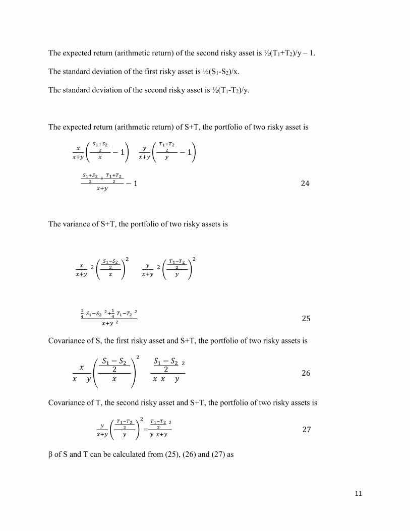
The expected return (arithmetic return) of the first risky asset is ½(S1+S2)/x – 1.
11
The expected return (arithmetic return) of the second risky asset is ½(T1+T2)/y – 1.
The standard deviation of the first risky asset is ½(S1-S2)/x.
The standard deviation of the second risky asset is ½(T1-T2)/y.
The expected return (arithmetic return) of S+T, the portfolio of two risky asset is
𝑥𝑥𝑥𝑥+𝑦𝑦
�(𝑆𝑆1+𝑆𝑆2)
2𝑥𝑥
− 1� + 𝑦𝑦𝑥𝑥+𝑦𝑦
�(𝑇𝑇1+𝑇𝑇2)
2𝑦𝑦
− 1�
=(𝑆𝑆1+𝑆𝑆2)
2 +(𝑇𝑇1+𝑇𝑇2)2
𝑥𝑥+𝑦𝑦− 1 (24)
The variance of S+T, the portfolio of two risky assets is
( 𝑥𝑥𝑥𝑥+𝑦𝑦
)2 �(𝑆𝑆1−𝑆𝑆2)
2𝑥𝑥
�2
+ ( 𝑦𝑦𝑥𝑥+𝑦𝑦
)2 �(𝑇𝑇1−𝑇𝑇2)
2𝑦𝑦
�2
=14
(𝑆𝑆1−𝑆𝑆2)2+14(𝑇𝑇1−𝑇𝑇2)2
(𝑥𝑥+𝑦𝑦)2 (25)
Covariance of S, the first risky asset and S+T, the portfolio of two risky assets is
𝑥𝑥𝑥𝑥 + 𝑦𝑦
�(𝑆𝑆1 − 𝑆𝑆2)
2𝑥𝑥
�
2
=(𝑆𝑆1 − 𝑆𝑆2
2 )2
𝑥𝑥(𝑥𝑥 + 𝑦𝑦) (26)
Covariance of T, the second risky asset and S+T, the portfolio of two risky assets is
𝑦𝑦𝑥𝑥+𝑦𝑦
�(𝑇𝑇1−𝑇𝑇2)
2𝑦𝑦
�2
=(𝑇𝑇1−𝑇𝑇22 )2
𝑦𝑦(𝑥𝑥+𝑦𝑦) (27)
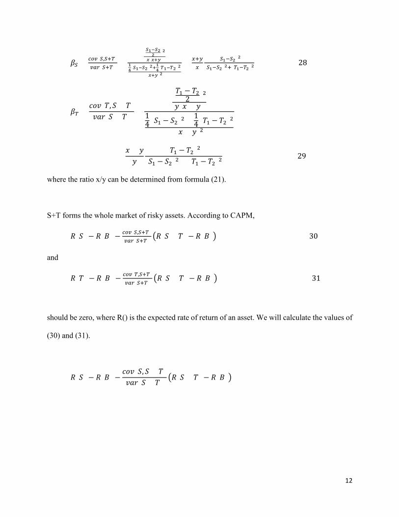
β of S and T can be calculated from (25), (26) and (27) as
12
𝛽𝛽𝑆𝑆 = 𝑐𝑐𝑐𝑐𝑣𝑣(𝑆𝑆,𝑆𝑆+𝑇𝑇)𝑣𝑣𝑣𝑣𝑣𝑣(𝑆𝑆+𝑇𝑇)
=(𝑆𝑆1−𝑆𝑆22 )2
𝑥𝑥(𝑥𝑥+𝑦𝑦)14(𝑆𝑆1−𝑆𝑆2)2+14(𝑇𝑇1−𝑇𝑇2)2
(𝑥𝑥+𝑦𝑦)2
= 𝑥𝑥+𝑦𝑦𝑥𝑥
(𝑆𝑆1−𝑆𝑆2)2
(𝑆𝑆1−𝑆𝑆2)2+(𝑇𝑇1−𝑇𝑇2)2 (28)
𝛽𝛽𝑇𝑇 =𝑐𝑐𝑐𝑐𝑣𝑣(𝑇𝑇, 𝑆𝑆 + 𝑇𝑇)𝑣𝑣𝑣𝑣𝑣𝑣(𝑆𝑆 + 𝑇𝑇)
=
(𝑇𝑇1 − 𝑇𝑇22 )2
𝑦𝑦(𝑥𝑥 + 𝑦𝑦)14 (𝑆𝑆1 − 𝑆𝑆2)2 + 1
4 (𝑇𝑇1 − 𝑇𝑇2)2
(𝑥𝑥 + 𝑦𝑦)2
=𝑥𝑥 + 𝑦𝑦𝑦𝑦
(𝑇𝑇1 − 𝑇𝑇2)2
(𝑆𝑆1 − 𝑆𝑆2)2 + (𝑇𝑇1 − 𝑇𝑇2)2 (29)
where the ratio x/y can be determined from formula (21).
S+T forms the whole market of risky assets. According to CAPM,
𝑅𝑅(𝑆𝑆) − 𝑅𝑅(𝐵𝐵) − 𝑐𝑐𝑐𝑐𝑣𝑣(𝑆𝑆,𝑆𝑆+𝑇𝑇)𝑣𝑣𝑣𝑣𝑣𝑣(𝑆𝑆+𝑇𝑇) �𝑅𝑅(𝑆𝑆 + 𝑇𝑇) − 𝑅𝑅(𝐵𝐵)� (30)
and
𝑅𝑅(𝑇𝑇) − 𝑅𝑅(𝐵𝐵) − 𝑐𝑐𝑐𝑐𝑣𝑣(𝑇𝑇,𝑆𝑆+𝑇𝑇)𝑣𝑣𝑣𝑣𝑣𝑣(𝑆𝑆+𝑇𝑇) �𝑅𝑅(𝑆𝑆 + 𝑇𝑇) − 𝑅𝑅(𝐵𝐵)� (31)
should be zero, where R() is the expected rate of return of an asset. We will calculate the values of
(30) and (31).
𝑅𝑅(𝑆𝑆) − 𝑅𝑅(𝐵𝐵) −𝑐𝑐𝑐𝑐𝑣𝑣(𝑆𝑆, 𝑆𝑆 + 𝑇𝑇)𝑣𝑣𝑣𝑣𝑣𝑣(𝑆𝑆 + 𝑇𝑇) �𝑅𝑅(𝑆𝑆 + 𝑇𝑇) − 𝑅𝑅(𝐵𝐵)�

13
= �(𝑆𝑆1 + 𝑆𝑆2)
2𝑥𝑥
− 1� − �𝐵𝐵𝑚𝑚− 1�
−
𝑥𝑥𝑥𝑥 + 𝑦𝑦 �
(𝑆𝑆1 − 𝑆𝑆2)2𝑥𝑥 �
2
14 (𝑆𝑆1 − 𝑆𝑆2)2 + 1
4 (𝑇𝑇1 − 𝑇𝑇2)2
(𝑥𝑥 + 𝑦𝑦)2
{�(𝑆𝑆1 + 𝑆𝑆2)
2 + (𝑇𝑇1 + 𝑇𝑇2)2
𝑥𝑥 + 𝑦𝑦− 1�
− �𝐵𝐵𝑚𝑚− 1�}
= �(𝑆𝑆1 + 𝑆𝑆2)
2𝑥𝑥
� − �𝐵𝐵𝑚𝑚� −
𝑥𝑥 + 𝑦𝑦𝑥𝑥 �𝑆𝑆1 − 𝑆𝑆2
2 �2
14 (𝑆𝑆1 − 𝑆𝑆2)2 + 1
4 (𝑇𝑇1 − 𝑇𝑇2)2{�
(𝑆𝑆1 + 𝑆𝑆2)2 + (𝑇𝑇1 + 𝑇𝑇2)
2𝑥𝑥 + 𝑦𝑦
� − �𝐵𝐵𝑚𝑚�}
= �(𝑆𝑆1 + 𝑆𝑆2)
2𝑥𝑥
� − �𝐵𝐵𝑚𝑚� −
�𝑆𝑆1 − 𝑆𝑆22 �
2
14 (𝑆𝑆1 − 𝑆𝑆2)2 + 1
4 (𝑇𝑇1 − 𝑇𝑇2)2{�
(𝑆𝑆1 + 𝑆𝑆2)2 + (𝑇𝑇1 + 𝑇𝑇2)
2𝑥𝑥
� − �𝐵𝐵𝑚𝑚𝑥𝑥 + 𝑦𝑦𝑥𝑥
�}
=1𝑥𝑥�
(𝑆𝑆1 + 𝑆𝑆2)2
− �𝐵𝐵𝑥𝑥𝑚𝑚�
−�𝑆𝑆1 − 𝑆𝑆2
2 �2
14 (𝑆𝑆1 − 𝑆𝑆2)2 + 1
4 (𝑇𝑇1 − 𝑇𝑇2)2��
(𝑆𝑆1 + 𝑆𝑆2)2
+(𝑇𝑇1 + 𝑇𝑇2)
2�
− �𝐵𝐵𝑚𝑚
(𝑥𝑥 + 𝑦𝑦)��� (32)

14
To keep the length of the formulas manageable, we will introduce four more short representations.
1° = 2′3′4′, 2° = 1′3′4′, 3° = 1′2′4′, 4° = 1′2′3′
From (22), (23), formula (32) will be
=1𝑥𝑥
{(𝑆𝑆1 + 𝑆𝑆2)
2− �
𝑆𝑆11° + 𝑆𝑆12° + 𝑆𝑆23° + 𝑆𝑆24°
1° + 2° + 3° + 4° �
−�𝑆𝑆1 − 𝑆𝑆2
2 �2
14 (𝑆𝑆1 − 𝑆𝑆2)2 + 1
4 (𝑇𝑇1 − 𝑇𝑇2)2[�
(𝑆𝑆1 + 𝑆𝑆2)2
+(𝑇𝑇1 + 𝑇𝑇2)
2�
−(𝑆𝑆1 + 𝑇𝑇1)1° + (𝑆𝑆1 + 𝑇𝑇2)2° + (𝑆𝑆2 + 𝑇𝑇1)3° + (𝑆𝑆2 + 𝑇𝑇2)4°
1° + 2° + 3° + 4° ]}
=1𝑥𝑥
11° + 2° + 3° + 4°
1(𝑆𝑆1 − 𝑆𝑆2)2 + (𝑇𝑇1 − 𝑇𝑇2)2 {
(𝑆𝑆1 + 𝑆𝑆2)2
(1° + 2° + 3° + 4°)((𝑆𝑆1 − 𝑆𝑆2)2
+ (𝑇𝑇1 − 𝑇𝑇2)2) − (𝑆𝑆11° + 𝑆𝑆12° + 𝑆𝑆23° + 𝑆𝑆24°)((𝑆𝑆1 − 𝑆𝑆2)2 + (𝑇𝑇1 − 𝑇𝑇2)2)
− (𝑆𝑆1 − 𝑆𝑆2)2[�(𝑆𝑆1 + 𝑆𝑆2)
2+
(𝑇𝑇1 + 𝑇𝑇2)2
� (1° + 2° + 3° + 4°)
− ((𝑆𝑆1 + 𝑇𝑇1)1° + (𝑆𝑆1 + 𝑇𝑇2)2° + (𝑆𝑆2 + 𝑇𝑇1)3° + (𝑆𝑆2 + 𝑇𝑇2)4°)]}
=1𝑥𝑥
11° + 2° + 3° + 4°
1(𝑆𝑆1 − 𝑆𝑆2)2 + (𝑇𝑇1 − 𝑇𝑇2)2 {(𝑇𝑇1 − 𝑇𝑇2)2 �
12
(𝑆𝑆1 + 𝑆𝑆2)(1° + 2° + 3° + 4°)
− (𝑆𝑆11° + 𝑆𝑆12° + 𝑆𝑆23° + 𝑆𝑆24°)� − (𝑆𝑆1 − 𝑆𝑆2)2[12
(𝑇𝑇1 + 𝑇𝑇2)(1° + 2° + 3° + 4°)
+ (𝑆𝑆11° + 𝑆𝑆12° + 𝑆𝑆23° + 𝑆𝑆24°)
− ((𝑆𝑆1 + 𝑇𝑇1)1° + (𝑆𝑆1 + 𝑇𝑇2)2° + (𝑆𝑆2 + 𝑇𝑇1)3° + (𝑆𝑆2 + 𝑇𝑇2)4°)

15
=1𝑥𝑥
11° + 2° + 3° + 4°
1(𝑆𝑆1 − 𝑆𝑆2)2 + (𝑇𝑇1 − 𝑇𝑇2)2 {(𝑇𝑇1 − 𝑇𝑇2)2 �
12
(𝑆𝑆1 + 𝑆𝑆2)(1° + 2° + 3° + 4°)
− (𝑆𝑆11° + 𝑆𝑆12° + 𝑆𝑆23° + 𝑆𝑆24°)�
− (𝑆𝑆1 − 𝑆𝑆2)2 �12
(𝑇𝑇1 + 𝑇𝑇2)(1° + 2° + 3° + 4°) − (𝑇𝑇11° + 𝑇𝑇22° + 𝑇𝑇13° + 𝑇𝑇24°�]}
=1𝑥𝑥
11° + 2° + 3° + 4°
1(𝑆𝑆1 − 𝑆𝑆2)2 + (𝑇𝑇1 − 𝑇𝑇2)2 {
12
(𝑇𝑇1 − 𝑇𝑇2)2[−(𝑆𝑆1 − 𝑆𝑆2)1° − (𝑆𝑆1 − 𝑆𝑆2)2°
+ (𝑆𝑆1 − 𝑆𝑆2)3° + (𝑆𝑆1 − 𝑆𝑆2)4°]
−12
(𝑆𝑆1 − 𝑆𝑆2)2[−(𝑇𝑇1 − 𝑇𝑇2)1° + (𝑇𝑇1 − 𝑇𝑇2)2° − (𝑇𝑇1 − 𝑇𝑇2)3° + (𝑇𝑇1 − 𝑇𝑇2)4°]}
=12
1𝑥𝑥
11° + 2° + 3° + 4°
(𝑆𝑆1 − 𝑆𝑆2)(𝑇𝑇1 − 𝑇𝑇2)(𝑆𝑆1 − 𝑆𝑆2)2 + (𝑇𝑇1 − 𝑇𝑇2)2 {(𝑇𝑇1 − 𝑇𝑇2)[−1° − 2° + 3° + 4°]
− (𝑆𝑆1 − 𝑆𝑆2)[−1° + 2° − 3° + 4°]}
12
1𝑥𝑥
11° + 2° + 3° + 4°
(𝑆𝑆1 − 𝑆𝑆2)(𝑇𝑇1 − 𝑇𝑇2)(𝑆𝑆1 − 𝑆𝑆2)2 + (𝑇𝑇1 − 𝑇𝑇2)2 {(𝑇𝑇1 − 𝑇𝑇2)[(𝑆𝑆1 − 𝑆𝑆2)2′4′ + (𝑆𝑆1 − 𝑆𝑆2)1′3′]
− (𝑆𝑆1 − 𝑆𝑆2)[(𝑇𝑇1 − 𝑇𝑇2)3′4′ + (𝑇𝑇1 − 𝑇𝑇2)1′2′]}
=12
1𝑥𝑥
11° + 2° + 3° + 4°
(𝑆𝑆1 − 𝑆𝑆2)2(𝑇𝑇1 − 𝑇𝑇2)2
(𝑆𝑆1 − 𝑆𝑆2)2 + (𝑇𝑇1 − 𝑇𝑇2)2 {[2′4′ + 1′3′] − [3′4′ + 1′2′]}
=12
1𝑥𝑥
11° + 2° + 3° + 4°
(𝑆𝑆1 − 𝑆𝑆2)2(𝑇𝑇1 − 𝑇𝑇2)2
(𝑆𝑆1 − 𝑆𝑆2)2 + (𝑇𝑇1 − 𝑇𝑇2)21𝐶𝐶
{[(𝐵𝐵 + 𝑆𝑆1 + 𝑇𝑇2)(𝐵𝐵 + 𝑆𝑆2 + 𝑇𝑇2)
+ (𝐵𝐵 + 𝑆𝑆1 + 𝑇𝑇1)(𝐵𝐵 + 𝑆𝑆2 + 𝑇𝑇1)] − [(𝐵𝐵 + 𝑆𝑆2 + 𝑇𝑇1)(𝐵𝐵 + 𝑆𝑆2 + 𝑇𝑇2)
+ (𝐵𝐵 + 𝑆𝑆1 + 𝑇𝑇1)(𝐵𝐵 + 𝑆𝑆1 + 𝑇𝑇2)] }
16
=12
1𝑥𝑥
11° + 2° + 3° + 4°
(𝑆𝑆1 − 𝑆𝑆2)2(𝑇𝑇1 − 𝑇𝑇2)2
(𝑆𝑆1 − 𝑆𝑆2)2 + (𝑇𝑇1 − 𝑇𝑇2)21𝐶𝐶
{(𝐵𝐵 + 𝑆𝑆2 + 𝑇𝑇2)(𝑆𝑆1 − 𝑆𝑆2 + 𝑇𝑇2 − 𝑇𝑇1)
− (𝐵𝐵 + 𝑆𝑆1 + 𝑇𝑇1)(𝑆𝑆1 − 𝑆𝑆2 + 𝑇𝑇2 − 𝑇𝑇1) }
=12
1𝑥𝑥
11° + 2° + 3° + 4°
(𝑆𝑆1 − 𝑆𝑆2)2(𝑇𝑇1 − 𝑇𝑇2)2
(𝑆𝑆1 − 𝑆𝑆2)2 + (𝑇𝑇1 − 𝑇𝑇2)21𝐶𝐶
{(𝑆𝑆2 + 𝑇𝑇2 − 𝑆𝑆1 − 𝑇𝑇1)(𝑆𝑆1 − 𝑆𝑆2 + 𝑇𝑇2 − 𝑇𝑇1)}
=12
1𝑥𝑥
11° + 2° + 3° + 4°
(𝑆𝑆1 − 𝑆𝑆2)2(𝑇𝑇1 − 𝑇𝑇2)2
(𝑆𝑆1 − 𝑆𝑆2)2 + (𝑇𝑇1 − 𝑇𝑇2)21𝐶𝐶
{(𝑇𝑇1 − 𝑇𝑇2)2 − (𝑆𝑆1 − 𝑆𝑆2)2}
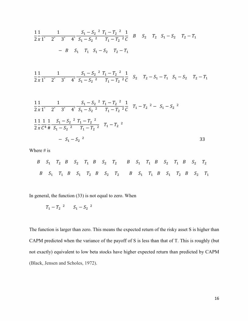
=12
1𝑥𝑥
1𝐶𝐶4
1#
(𝑆𝑆1 − 𝑆𝑆2)2(𝑇𝑇1 − 𝑇𝑇2)2
(𝑆𝑆1 − 𝑆𝑆2)2 + (𝑇𝑇1 − 𝑇𝑇2)2{(𝑇𝑇1 − 𝑇𝑇2)2
− (𝑆𝑆1 − 𝑆𝑆2)2} (33)
Where # is
(𝐵𝐵 + 𝑆𝑆1 + 𝑇𝑇2)(𝐵𝐵 + 𝑆𝑆2 + 𝑇𝑇1)(𝐵𝐵 + 𝑆𝑆2 + 𝑇𝑇2) + (𝐵𝐵 + 𝑆𝑆1 + 𝑇𝑇1)(𝐵𝐵 + 𝑆𝑆2 + 𝑇𝑇1)(𝐵𝐵 + 𝑆𝑆2 + 𝑇𝑇2) +
(𝐵𝐵 + 𝑆𝑆1 + 𝑇𝑇1)(𝐵𝐵 + 𝑆𝑆1 + 𝑇𝑇2)(𝐵𝐵 + 𝑆𝑆2 + 𝑇𝑇2) + (𝐵𝐵 + 𝑆𝑆1 + 𝑇𝑇1)(𝐵𝐵 + 𝑆𝑆1 + 𝑇𝑇2)(𝐵𝐵 + 𝑆𝑆2 + 𝑇𝑇1)
In general, the function (33) is not equal to zero. When
(𝑇𝑇1 − 𝑇𝑇2)2 > (𝑆𝑆1 − 𝑆𝑆2)2
The function is larger than zero. This means the expected return of the risky asset S is higher than
CAPM predicted when the variance of the payoff of S is less than that of T. This is roughly (but
not exactly) equivalent to low beta stocks have higher expected return than predicted by CAPM
(Black, Jensen and Scholes, 1972).
17
3. Numerical calculations
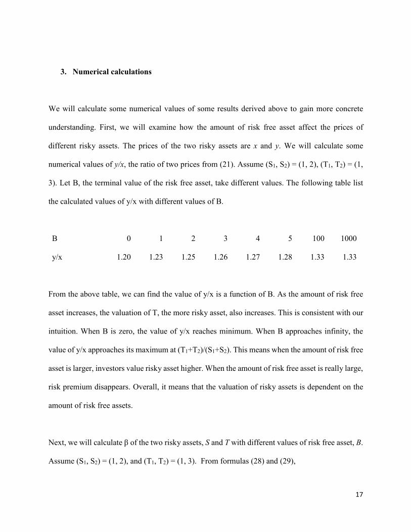
We will calculate some numerical values of some results derived above to gain more concrete
understanding. First, we will examine how the amount of risk free asset affect the prices of
different risky assets. The prices of the two risky assets are x and y. We will calculate some
numerical values of y/x, the ratio of two prices from (21). Assume (S1, S2) = (1, 2), (T1, T2) = (1,
3). Let B, the terminal value of the risk free asset, take different values. The following table list
the calculated values of y/x with different values of B.
B 0 1 2 3 4 5 100 1000
y/x 1.20 1.23 1.25 1.26 1.27 1.28 1.33 1.33
From the above table, we can find the value of y/x is a function of B. As the amount of risk free
asset increases, the valuation of T, the more risky asset, also increases. This is consistent with our
intuition. When B is zero, the value of y/x reaches minimum. When B approaches infinity, the
value of y/x approaches its maximum at (T1+T2)/(S1+S2). This means when the amount of risk free
asset is larger, investors value risky asset higher. When the amount of risk free asset is really large,
risk premium disappears. Overall, it means that the valuation of risky assets is dependent on the
amount of risk free assets.
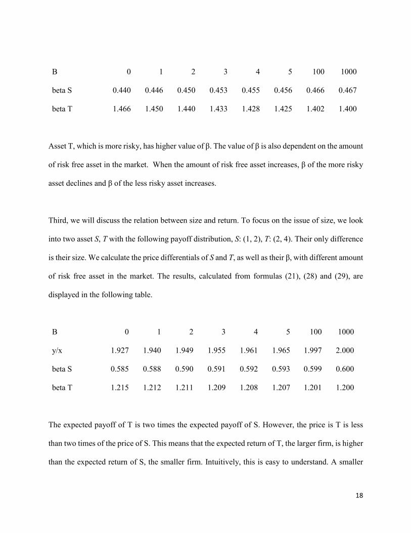
Next, we will calculate β of the two risky assets, S and T with different values of risk free asset, B.
Assume (S1, S2) = (1, 2), and (T1, T2) = (1, 3). From formulas (28) and (29),
18
B 0 1 2 3 4 5 100 1000
beta S 0.440 0.446 0.450 0.453 0.455 0.456 0.466 0.467
beta T 1.466 1.450 1.440 1.433 1.428 1.425 1.402 1.400
Asset T, which is more risky, has higher value of β. The value of β is also dependent on the amount
of risk free asset in the market. When the amount of risk free asset increases, β of the more risky
asset declines and β of the less risky asset increases.
Third, we will discuss the relation between size and return. To focus on the issue of size, we look
into two asset S, T with the following payoff distribution, S: (1, 2), T: (2, 4). Their only difference
is their size. We calculate the price differentials of S and T, as well as their β, with different amount
of risk free asset in the market. The results, calculated from formulas (21), (28) and (29), are
displayed in the following table.
B 0 1 2 3 4 5 100 1000
y/x 1.927 1.940 1.949 1.955 1.961 1.965 1.997 2.000
beta S 0.585 0.588 0.590 0.591 0.592 0.593 0.599 0.600
beta T 1.215 1.212 1.211 1.209 1.208 1.207 1.201 1.200
The expected payoff of T is two times the expected payoff of S. However, the price is T is less
than two times of the price of S. This means that the expected return of T, the larger firm, is higher
than the expected return of S, the smaller firm. Intuitively, this is easy to understand. A smaller
19
firm has higher diversification value. So it is over weighted in value relative to its payoff. This
causes its expected rate of return to be lower. But why in Fama-French three factor model, small
firms has positive loading? We need to look at the values of β. The β of S, the smaller firm, is
much smaller than that of T, the larger firm. So according to CAPM, the expected rate of return of
S is much lower than that of T. The positive loading of firm size in Fama-French three factor model
partially offset this problem. But it does not mean smaller firms provide higher rate of return.
Currently, empirical evidence on size and return in inconclusive (Van Dijk, 2011).
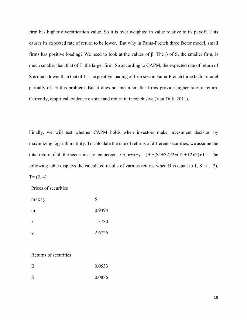
Finally, we will test whether CAPM holds when investors make investment decision by
maximizing logarithm utility. To calculate the rate of returns of different securities, we assume the
total return of all the securities are ten percent. Or m+x+y = (B +(S1+S2)/2+(T1+T2)/2))/1.1. The
following table displays the calculated results of various returns when B is equal to 1, S= (1, 2),
T= (2, 4).
Prices of securities
m+x+y
5
m
0.9494
x
1.3780
y
2.6726
Returns of securities
B
0.0533
S
0.0886

20
T
0.1225
S+T
0.1109
Risk premiums
S+T-B
0.0577
S-B
0.0353
T-B
0.0692
Test of CAPM
S-B- βS*(S+T-B)
0.0014
T-B- βT*(S+T-B)
-0.0007
If CAPM model is valid, the last two terms should be zero. But among these two terms, the first,
representing the smaller firm, is positive, the second, representing the larger firm, is negative. This
means small firms has higher return and large firms has lower return than predicted by CAPM.
This is consistent with statistical results obtained by Fama and French (1993).
4. Concluding remarks
In CAPM, it is assumed that investors maximize their utility. We construct a very simple asset
market. Then we apply the utility theory to calculate the return and variance of different assets.
The results are different from that from CAPM. This shows that the theory of CAPM is internally
inconsistent. Furthermore, the theoretical results derived from the utility theory are more consistent

21
with market data. The methodology in this work can be extended to general asset markets. The
same methodology can be applied to other utility functions as well.
22
References
Black, Fischer, Michael C. Jensen, and Myron Scholes. 1972, "The Capital Asset Pricing Model:
Some Empirical Tests." In Studies in the Theory of Capital Markets, edited by M. C. Jensen. New
York: Praeger,
Chen, J. 2010, Where is the Efficient Frontier, EuroEconomica, Vol 24, No 1, 22-26.
Fama, E.F. and French, K.R., 1993. Common risk factors in the returns on stocks and
bonds. Journal of financial economics, 33(1), pp.3-56.
Fama, E.F. and French, K.R., 2004, The Capital Asset Pricing Model: Theory and Evidence,
Journal of Economic Perspective
Lintner, J., 1965. The valuation of risk assets and the selection of risky investments in stock
portfolios and capital budgets. The review of economics and statistics, pp.13-37.
Mehra, R. and Prescott, E.C., 1985. The equity premium: A puzzle. Journal of monetary
Economics, 15(2), pp.145-161.
Sharpe, W.F., 1964. Capital asset prices: A theory of market equilibrium under conditions of
risk. The journal of finance, 19(3), pp.425-442.
Van Dijk, M.A., 2011. Is size dead? A review of the size effect in equity returns. Journal of
Banking & Finance, 35(12), pp.3263-3274.