Embed Size (px)
Citation preview

ON THE IMPLICIT INTEGRATION OF DIFFERENTIAL-ALGEBRAIC
EQUATIONS OF MULTIBODY DYNAMICS
by
Dan Negrut
A thesis submitted in partial fulfillmentof the requirements for the Doctor of
Philosophy degree in Mechanical Engineeringin the Graduate College of
The University of Iowa
July 1998
Thesis supervisor: Professor Edward J. Haug

Graduate CollegeThe University of Iowa
Iowa City, Iowa
CERTIFICATE OF APPROVAL
_______________________
PH.D. THESIS
____________
This is to certify that the Ph.D. thesis of
Dan Negrut
has been approved by the Examining Committeefor the thesis requirement for the Doctor ofPhilosophy degree in Mechanical Engineering at the July 1998 graduation.
Thesis committee: ______________________________________Thesis supervisor
______________________________________Member
______________________________________Member
______________________________________Member
______________________________________Member

ii
To my parents

iii
ACKNOWLEDGMENTS
I would like to thank my advisor Professor Edward J. Haug for his continuous
guidance, I learned many worthwhile things from him. I would also like to thank
Professor Florian A. Potra, for his advice and help over the last 5 years and Professor
Jeffrey S. Freeman for his patience and understanding during my early years at The
University of Iowa.
My thanks and good thoughts go to Cristina, for always supporting and
encouraging me, and to Feli, for providing inspiration and always cheering me up.
I am deeply grateful to my teachers and my friends.

iv
ABSTRACT
The topic of the thesis is implicit integration of the differential-algebraic
equations (DAE) of Multibody Dynamics. Methods used in the thesis for the solution of
DAE are based on state-space reduction via generalized coordinate partitioning. In this
approach, a subset of independent generalized coordinates , equal in number to the
number of degrees of freedom of the mechanical system, is used to express the time
evolution of the mechanical system. The second order state-space ordinary differential
equations (SSODE) that describe the time variation of independent coordinates are
numerically integrated using implicit formulas. Efficient means for acceleration and
integration Jacobian computation are proposed and numerically implemented.
Methods proposed for numerical solution of the index 3 DAE of Multibody
Dynamics are the State-Space Reduction Method, the Descriptor Form Method, and the
First Order Reduction Method. Algorithms based on the State-Space Reduction and
Descriptor Form Methods employ the extensively used family of Newmark multi-step
formulas for implicit integration of the SSODE. More refined Runge-Kutta formulas are
used in conjunction with both First Order Reduction and Descriptor Form Methods.
Rosenbrock-Nystrom and SDIRK formulas of order 4 that are employed are L-stable
methods with sound stability and accuracy properties. All integration formulas are
provided with robust error control mechanisms based on integration step-size selection.
Several algorithms are developed, based on the proposed methods for numerical
solution of index 3 DAE of Multibody Dynamics. These algorithms are shown to be
robust and accurate. Typically, two orders of magnitude speed-up is achieved when these
algorithms are compared to previously used, well established, explicit numerical

v
integration algorithms for simulation of a stiff model of the High Mobility Multipurpose
Wheeled Vehicle (HMMWV) of the US Army.
Computational methods developed in this thesis enable efficient dynamic analysis
of systems containing bushings, stiff subsystem compliance elements, and high frequency
subsystems that heretofore required tremendous amounts of CPU time, due to limitations
of the previously employed numerical algorithms.

vi
TABLE OF CONTENTS
Page
LIST OF TABLES ...................................................................................................... viii
LIST OF FIGURES..................................................................................................... x
CHAPTER
1. INTRODUCTION...................................................................................... 1
1.1. Motivation............................................................................ 11.2. Thesis Overview................................................................... 2
2. REVIEW OF LITERATURE..................................................................... 5
2.1. Review of Methods for the Solution of DAE....................... 52.2. Review of Methods for the Solution of ODE....................... 19
3. THEORETICAL CONSIDERATIONS..................................................... 31
3.1. Generalized Coordinates Partitioning Algorithm................. 313.2. State-Space Reduction Method............................................ 35
3.2.1. Multi-step Methods ................................................. 353.2.2. Runge-Kutta Methods ............................................. 44
3.3. Descriptor Form Method...................................................... 513.3.1. Multi-step Methods ................................................. 563.3.2. Runge-Kutta Methods ............................................. 56
3.4. First Order Reduction Method ............................................. 583.4.1. Theoretical Considerations in First Order
Reduction .................................................................. 593.4.2. Computing Accelerations in the Cartesian
Representation........................................................... 683.4.3. Computing Accelerations in Minimal
Representation........................................................... 84
4. NUMERICAL IMPLEMENTATIONS ..................................................... 111
4.1. Trapezoidal-Based State-Space Implicit Integration ........... 1114.1.1. General Considerations ........................................... 1114.1.2. Algorithm Pseudo-code ........................................... 112
4.2. SDIRK Based Descriptor Form Implicit Integration ........... 1184.2.1. General Considerations ........................................... 1184.2.2. SDIRK4/16 .............................................................. 1234.2.3. Algorithm Pseudo-code ........................................... 127
4.3. Trapezoidal-Based Descriptor Form Implicit Integration.... 131

vii
4.3.1. Algorithm Pseudo-code ........................................... 1314.4. Rosenbrock-Based First Order Implicit Integration............. 133
4.4.1. General Consideration ............................................. 1334.4.2. Rosenbrock-Nystrom Methods................................ 1354.4.3. Order Conditions For Rosenbrock-Nystrom
Algorithm.................................................................. 1424.4.4. Algorithm Pseudo-code ........................................... 148
4.5. SDIRK-Based First Order Implicit Integration.................... 1534.5.1. SDIRK4/15 .............................................................. 1534.5.2. Algorithm Pseudo-code ........................................... 159
5. NUMERICAL EXPERIMENTS................................................................ 165
5.1. Validation of First Order Reduction Method....................... 1655.2. Explicit versus Implicit Integration...................................... 1745.3. Method Comparison............................................................. 182
6. CONCLUSIONS AND RECOMMENDATIONS..................................... 192
APPENDIX A. PARALLEL COMPUTATION OF INTEGRATIONJACOBIAN..................................................................................... 194
APPENDIX B. TANGENT-PLANE PARAMETRIZATION-BASED IMPLICITINTEGRATION ............................................................................. 200
REFERENCES ........................................................................................................ 209

viii
LIST OF TABLES
Table Page
1. Butcher’s Tableau ....................................................................................... 44
2. Numerical Results: Solving For Accelerations andLagrange Multipliers................................................................................... 82
3. Timing Results for Seven Body Mechanism .............................................. 83
4. Timing Results for Chain of Pendulums..................................................... 83
5. HMMWV14 Model - Component Bodies .................................................. 105
6. Operation Count for Gaussian Elimination................................................. 107
7. Operation Count for Alg-S .......................................................................... 108
8. Operation Count for Alg-D ......................................................................... 109
9. JR Linear Solvers CPU Results .................................................................. 109
10. Timing Profiles – Alg-S and Alg-D ............................................................. 110
11. Pseudo-code for Trapezoidal-Based State-Space Method.......................... 113
12. Butcher’s Tableau for SDIRK Formulas .................................................... 124
13. SDIRK4/16 Formula for Descriptor Form Method .................................... 126
14. Pseudo-code for SDIRK4/16-Based Descriptor Form Method .................. 128
15. Pseudo-code for Trapezoidal-Based Descriptor Form Method .................. 132
16. Pseudo-code for Rosenbrock-Nystrom-Based First Order ReductionMethod ........................................................................................................ 149
17. Pseudo-code for SDIRK4/15-Based First Order Reduction Method.......... 160
18. Parameters for the Double Pendulum ......................................................... 165
19. Initial Conditions for Double Pendulum..................................................... 166

ix
20. Position Error Analysis ForSDIRK............................................................. 170
21. Position Error Analysis ForRosen .............................................................. 171
22. Velocity Error Analysis ForSDIRK ............................................................ 173
23. Velocity Error Analysis ForRosen.............................................................. 174
24. HMMWV14 Explicit Integration Simulation CPU Times ......................... 178
25. HMMWV14 Implicit Integration Simulation Results ................................ 179
26. Timing Results for InflSDIRK .................................................................... 183
27. Timing Results for InflTrap ........................................................................ 183
28. Timing Results for ForSDIRK .................................................................... 183
29. Timing Results for ForRosen...................................................................... 184
30. ForSDIRK Analytical/Numerical Computation of Integration Jacobian.... 191
31. Pseudo-code for Parallel Computation of Integration Jacobian ................. 197

x
LIST OF FIGURES
Figure Page
1. Seven Body Mechanism ............................................................................. 69
2. Chain of Pendulums.................................................................................... 76
3. Graph Representation: Seven-Body Mechanism........................................ 76
4. Reduced Matrix B: Seven-Body Mechanism ............................................. 77
5. Two Joint Numbering Schemes: Chain of Pendulums ............................... 78
6. Reduced Matrix: Chain of Pendulums........................................................ 78
7. A Pair of Connected Bodies in JR .............................................................. 86
8. A Tree Structure.......................................................................................... 90
9. HMMWV14 Body Model: Topology Graph .............................................. 105
10. Spanning Tree – HMMWV14 .................................................................... 106
11. Double Pendulum........................................................................................ 166
12. Orientation Body 1...................................................................................... 169
13. Angular Velocity Body 1 ............................................................................ 172
14. US Army HMMWV ................................................................................... 175
15. 14 Body Model of HMMWV ..................................................................... 175
16. Topology Graph for HMMWV14............................................................... 176
17. Chassis Height HMMWV14....................................................................... 177
18. Explicit Integration Results for Tolerance 10-3........................................... 180
19. Implicit Integration Results for Tolerance 10-3........................................... 181
20. Timing Results for Different Tolerances .................................................... 181

xi
21. Algorithm Comparison for Different Tolerances ....................................... 186
22. Algorithm Comparison for Different Simulation Lengths.......................... 187
23. Step-Size History for ForSDIRK and SspTrap ........................................... 188
24. Step-Size History for ForRosen and InflSDIRK ......................................... 189
25. Number of Iterations for SspTrap ............................................................... 191

1
CHAPTER 1
INTRODUCTION
1.1 Motivation
The motivation for this thesis lies in the importance of having effective
mathematical and computational tools for virtual prototyping. In a world of increasing
global competition and shrinking windows of opportunity, as design cycles are
continuously compressed under the pressure of high quality standards and short time-to-
market objectives, virtual prototyping becomes a powerful tool in the hands of designers.
Once the privilege of few companies, steady growth in inexpensive computational power
has established virtual prototyping as an essential link in the design cycle of virtually any
successful company. In applications ranging from Aircraft and Automotive Industries, to
Biomechanics and Mechatronics, cutting costs and reducing development cycles by
eliminating hardware prototypes, along with quality improvement through design
sensitivity and “what-if” studies are attributes that have made virtual prototyping an
important segment of CAE/CAD/CAM integrated environments.
With these considerations in mind, at the beginning of 1996, the writer critically
evaluated some of the mathematical methods of virtual prototyping in Multibody
Dynamics. Research topics were identified that had the potential to qualitatively improve
methods in use at that time. A first goal was to answer the challenge posed by dynamic
analysis of richer and more complex dynamic systems, and then there was the objective
of developing algorithms and methods that would enable effective numerical
implementations of theoretical methods once deemed to be computationally intractable.
2
Computational stability and efficiency were the key issues, to be addressed using new
algorithms for topology-based linear algebra and numerical integration of Differential-
Algebraic Equations of Multibody Dynamics.
1.2 Thesis Overview
This Section provides an outline of the thesis. Brief remarks describe the content
of each Chapter of the thesis.
Chapter 2 contains a review of the literature. Many different techniques for the
solution of differential-algebraic equations (DAE) of Multibody Dynamics have been
proposed over time. Some of the more important approaches are presented, pointing out
their merits and deficiencies.
Chapter 3 contains the methods proposed for implicit numerical integration of
DAE of multibody dynamics. The first method presented is the State Space Reduction
Method, in which the DAE of Multibody Dynamics are reduced, via generalized
coordinate partitioning (Wehage and Haug, 1982), to a set of ordinary differential
equations (ODE).
The next method is the Descriptor Form Method, in which using an ODE
numerical integration formula, the index one DAE problem obtained by associating the
equations of motion and acceleration kinematic constraints equation, is directly
integrated. Constraint error accumulation is prevented in this method by recovering
dependent positions and velocities via position and velocity kinematic constraint
equations.
The last method presented for the solution of stiff DAE of Multibody Dynamics is
the First Order Reduction Method, which has the potential of using any standard implicit
numerical code to numerically solve the resulting ODE problem. In this formulation,

3
second order differential equations governing the time evolution of independent positions
is reduced to a system of first order differential equations. Central to the First Order
Reduction Method is the issue of generalized acceleration computation. Sections 3.4.2
and 3.4.3 are devoted to a comprehensive analysis of generalized acceleration
computation in Cartesian and minimal coordinates representations, respectively.
Based on theoretical considerations of Chapter 3, several algorithms and codes
were developed for the implicit integration of the DAE of Multibody Dynamics. These
codes represent numerical implementation of the State Space, Descriptor Form, and First
Order Reduction methods introduced in Sections 3.2, 3.3, and 3.4, respectively. The
codes are presented in Chapter 4. The methods implemented are as follows:
(a). The State Space Method is implemented based on the Newmark family of implicit
integration formulas. In particular, the Trapezoidal formula is used throughout the
numerical experiments, due to its higher order compared to other Newmark
formulas.
(b). The Descriptor Form Method is implemented based on two integration formulas
(b1). Trapezoidal formula.
(b2). A five stage, order 4, A-stable, stiffly-accurate singly diagonal implicit
Runge-Kutta (SDIRK) method.
(c). The first order approach was implemented using two different integration formulas
(c1). A four stage, order 4 Rosenbrock formula.
(c2). An SDIRK five stage, order 4, A-stable, stiffly-accurate formula of Hairer and
Wanner (1996).
When applicable, each numerical implementation is detailed in the following three
aspects:
(1). Specifics of DAE-to-ODE reduction.

4
(2). ODE integration stage.
(3). Iteration stopping criteria, and step size control.
Based on the algorithms developed, numerical experiments are carried out using
two test problems. Chapter 5 contains the results of these simulations. First, the
numerical methods are validated in terms of asymptotic behavior. Then, the implicit
integrators defined are compared in terms of efficiency with an explicit alternative for
integration of stiff ODE of Multibody Dynamics. A third set of numerical experiments is
aimed at comparing the implicit integrators among themselves.
Chapter 6 presents potential directions of future research, and concludes the thesis
with final remarks concerning the topic of generalized coordinate-based state-space
implicit integration of DAE of Multibody Dynamics. Appendix A presents more recent
theoretical results regarding the potential of using multiprocessor architectures for
speeding up the otherwise computationally intensive task of DAE implicit integration.
Fast integration Jacobian evaluation is the focus of the analysis in this Section, which
concludes with a strategy that can take advantage of parallel computer architectures.
Finally, the theoretical framework derived for the coordinate partitioning approach to
solving DAE of Multibody Dynamics is extended in Appendix B to the tangent-plane
parametrization method. In this context, coordinate partitioning is in fact a particular
case of the tangent-plane parametrization method, obtained by choosing a certain
projection matrix.

5
CHAPTER 2
REVIEW OF LITERATURE
2.1 Review of Methods for the Solution of DAE
In the present work, only the case of rigid body mechanical system models is
considered. However, the methods proposed in this work are suitable for dynamic
analysis of models incorporating flexible components. The issue of generating derivative
information specific to systems containing flexible components has not yet been
addressed.
Throughout this document, q = [ , , , ]q q qn1 2 K T denotes the vector of generalized
coordinates. The n generalized coordinates qi define the state of the mechanical system
at the position level; i.e., given a set of n values for qi , the position of each element of
the mechanical system model is uniquely determined. The generalized coordinates may
be absolute (Cartesian) coordinates of body reference frames, relative coordinates
between bodies, or a combination of both. Generalized velocities are defined as the first
time derivative of the generalized coordinates. In what follows an over-dot signifies time
derivative. Thus, generalized velocity is defined as
& [ & , & , , & ]q = q q qn1 2 K T (2.1)
The set of generalized positions and velocities define the state of the mechanical
system model; i.e., once these quantities are available there is a unique configuration of
the system at a given instant in time. Conversely, to each state of the mechanical system
there corresponds unique generalized position q and velocity &q.
6
Joints connecting bodies of a mechanical system model restrict the relative and/or
absolute motion of components of the model. From a mathematical standpoint, these
mobility constraints are accounted for by the requirement that a set of algebraic
expressions must be satisfied throughout the simulation. In the most general case, the
constraints may be equalities or inequalities involving generalized coordinates and their
first time derivatives. In this thesis only the case of scleronomic and holonomic equality
constraints will be considered; i. e., the constraint equations do not depend explicitly on
time, and they do not contain any time derivatives of generalized coordinates. Inequality
constraint equations are not treated in the thesis. Technically, this scenario can be
addressed by considering event driven integration of DAE, when event location
(discontinuity treatment) becomes the main issue of concern. More information about
event driven integration can be found in the work of Winckler (1997).
Under the above assumptions, the position kinematic constraint equations assume
the form
Φ( ) [ ( ), ( ), , ( )]q q q q 0≡ =Φ Φ Φ1 2 K mT (2.2)
Differentiating the position kinematic constraint equation of Eq. (2.2) with respect to time
yields the velocity kinematic constraint equation,
Φq q q 0( ) & = (2.3)
where subscripts denote partial differentiation; i.e., Φq = ∂Φ ∂[( ) / ( )]i jq . Finally, taking
another time derivative of Eq. (2.3) yields the acceleration kinematic equation,
Φ Φq q qq q q q q q( )&& ( & ) & ( , & )= - ¢ τ (2.4)
Equations (2.1) through (2.4) characterize the admissible motion of the constrained
mechanical system at position, velocity, and acceleration levels.

7
The state of the mechanical system will change in time under the effect of both
applied and constraint forces. The Lagrange multiplier form of the equations of motion
for the mechanical system model is (Haug , 1989)
M q q q Q q qq( )&& ( ) ( , & , )+ =ΦT Aλ t (2.5)
where M ∈ℜ ×n n is the mass matrix, which depends on the generalized coordinates q ;
λ ∈ℜm is the vector of Lagrange multipliers that account for the workless constraint
forces; and QA ∈ℜn is the vector of generalized applied forces that may depend on
generalized coordinates, their time derivatives, and time.
Equations (2.2) through (2.5) are the so-called Newton-Euler constrained
equations of motion. From a mathematical standpoint, they comprise a system of
differential-algebraic equations (DAE). Mathematically, DAE are not ODE (Petzold ,
1982). The task of obtaining a numerical solution of the DAE problem of Eqs. (2.2)
through (2.5) is substantially more difficult and prone to intense numerical computation
that the task of solving an ODE (Potra, 1994). This trend is more pronounced for higher
index DAE, where the index (Brenan, Campbell, Petzold, 1989), is defined as the number
of derivatives required to transform the DAE problem into an ODE problem.
To find the index of the DAE of Multibody Dynamics, note that acceleration
kinematic constraint equation of Eq. (2.4) is obtained after taking two time derivatives of
the position kinematic constraint equation of Eq. (2.2). The acceleration kinematic
equations are associated with the equations of motion to obtain a linear system in
generalized accelerations and Lagrange multipliers
M q Qq
q
ΦΦ
T A
0
�!
"$##�!
"$# =
�!
"$#
&&
λ τ(2.6)
The expression obtained for Lagrange multipliers, by formally solving Eq. (2.6), is a
function of generalized positions and velocities, q and &q , respectively. Taking a third

8
derivative of Lagrange multipliers, and combining these derivatives with Eq. (2.5),
results in a set of ODE. Consequently, the index of the DAE of Multibody Dynamics is
three.
In practice this sequence of steps converting the DAE to ODE is never used to
obtain the numerical solution of the original problem. Its only purpose is to determine
the index of the DAE being analyzed. This information is useful, as generally the index
is regarded as a measure of the difficulty that should be expected when numerically
solving the DAE. In particular, the index 3 of the DAE of Multibody Dynamics is a
rather high index when compared with DAE obtained from modeling problems arising in
other areas of Physics and Engineering.
Dynamic analysis of mechanical systems concerns their time evolution under the
action of applied forces. It is highly unlikely to obtain an analytical solution to the DAE
of Multibody Dynamics, so approximate solutions are obtained by means of numerical
methods. In this context, Eqs. (2.2) and (2.5) alone cease to characterize the time
evolution of the system, since Eqs. (2.3) and (2.4) are not guaranteed to be satisfied.
When this is the case, numerical solution at velocity and acceleration levels drifts away
from analytical solution. Consequently, future position configurations of the system will
be wrong, since the numerical integration stage embedded in the numerical algorithm
uses corrupted derivative information.
Special numerical methods have been developed to deal with DAE, and the theory
surrounding these methods builds around the index of the DAE. Thus, different
numerical methods are proposed for different index DAE problems. In this Section, the
focus is on methods for the solution of the index 3 DAE of Multibody Dynamics. Most
of the methods for the solution of this class of DAE belong to one of the following
categories:

9
(a). Stabilization Methods
(b). Projection Methods
(c). State Space Methods
An early stabilization-based numerical algorithm that allows for integration of
DAE is the so called constraint stabilization technique (Baumgarte, 1972). The problem
is reduced to index 1, as in Eq. (2.6), and is directly integrated. Since, after direct
integration the constraints fail to be satisfied, at the next time step, the right-side of
acceleration kinematic constraint equation is modified to take into account the constrain
violation.
The form of the right side acceleration kinematic constraint equation is altered to
τ τ= − −2α β&Φ Φ (2.7)
where last two terms are the so called compensation terms. These two terms do not
appear in the original form of acceleration kinematic constraint equation of Eq. (2.4), and
they compensate for errors in satisfying constraint equations at position and velocity
levels.
Ostermeyer (1990) discusses criteria for optimally choosing the positive scalars
α and β . This process is problematic (Ascher et. al, 1995) and is yet to be resolved.
Usually, α γ= and β γ= 2 where γ > 0 . The manifold then becomes an attractor of the
solution of the newly obtained system of ordinary differential equations of Eqs. (2.5) and
(2.7). Ideally, the value of the scalar γ would be independent of both the method used to
discretized the new set of ODE and the integration step-size. A simple example shows,
however, that choosing an optimal γ depends on both these factors.
Consider for example the hypothetical case of a system with linear constraints at
the position level,
Φ( )q Gq= (2.8)

10
Using the forward Euler integration formula, Baumgarte’s technique results in
& & ( , & ) ( )
[ ( , & ) & ]
&
q q M Q q q M G GM G
GM Q q q Gq Gq
q q q
n n n n
n n n n
n n n
h h
h
+
- - - -
-
+
= + -
¿ + += +
11 1 1 1
1
1
T T
α β (2.9)
In order to see how constraint equations are satisfied at the new time step n +1 , multiply
the new positions and velocities by G to obtain
$
&$ ( )
$
&$q
q
I I
I I
q
qn
n
n
n
h
h h+
+
�!
"$# = - -
�!
"$#�!
"$#
1
1 1α β(2.10)
where $q Gq≡ and &$ &q Gq≡ are errors in constraints at the position and velocity levels,
and I is the m m× identity matrix. Denoting by B the coefficient matrix in Eq. (2.10),
ideally B 0≡ . Since this is not possible for the forward Euler method, α and β are
optimally chosen; i. e., such that B 02 ≡ . These optimal values are α = 1 h and
β = 1 2h . In other words, the scalar γ above depends on both the method used to
discretize the ordinary differential equations and the integration step size, which is a
drawback of the approach.
More sophisticated techniques should be considered. Asher et al. (1995) propose
several algorithms that have as starting point the underlying ODE associated with the
index 3 DAE of Multibody Dynamics. The underlying ODE is obtained by formally
eliminating Lagrange multipliers from equations of motion of Eq. (2.5) using acceleration
kinematic constraint equation to obtain
λ τ= −− − −( ) [ ]Φ Φq q qM M Q1 1 1ΦT A (2.11)
Lagrange multipliers are substituted back into Eq. (2.5) to obtain the underlying ODE
associated to the DAE as
Mq Q q q M M Q q q q qq q q q&& ( , & ) ( ) [ ( , & ) ( , & )]= − −− − −A T T AΦ ΦΦ Φ1 1 1 τ (2.12)

11
which theoretically, can be further transformed to a first order system of ODE
& $( )z f z= (2.13)
with z q q≡ ( , & )T T T . By directly integrating the set of second order ODE in Eq. (2.12),
kinematic constraint equations at position and velocity levels will cease to be satisfied.
In the spirit of Baumgarte’s method, the idea of Ascher et al. (1995) is to add a
more general constraint stabilization term in right-side of Eq. (2.13), to obtain
& $( ) ( ) ( )z f z F z h z= − γ (2.14)
where γ > 0 is a parameter, F z( ) is a 2 2n m× matrix, and
h zq
( )( )
&=
�!
"$#
ΦΦ
(2.15)
are the kinematic constraint equations at position and velocity levels. In a numerical
implementation, the system of ODE of Eq. (2.14) is directly integrated by any explicit
integration scheme to advance the simulation.
While in Baumgarte’s method the parameters α and β were to be chosen, the
approach proposed by Ascher needs to provide the matrix F z( ) of Eq. (2.14). The
authors suggested several forms for this matrix. Based on simulation results of two
small-scale planar mechanical models, they concluded the approach is reliable for
nonstiff and highly oscillatory problems.
The addition of a stabilization term is not justified from a physical, but only a
mathematical standpoint; i. e., it is introduced to limit the drifting effect induced by direct
integration of all generalized coordinates in the formulation. Depending on the value of
the parameter γ and the expression of the compensation coefficient matrix F z( ) , the
dynamics of the system would be altered if the formulation of Eq. (2.14) is directly
integrated. Consequently, Ascher et al. slightly modify the proposed approach as

12
follows: First, use an integrator of choice to directly integrate the underlying ODE
reformulated as in Eq. (2.13). Then use Eq. (2.14) to stabilize the constraint equations.
In this respect this approach is very similar to coordinate projection techniques presented
later in this Section. Finally, the constraint stabilization algorithm proposed is as follows:
(1). Apply direct integration to the underlying ODE
~ ( )z zn hf
n+ =1 Ψ (2.16)
(2). Apply stabilization
z z F z h zn n n nh+ + + += −1 1 1 1~ (~ ) (~ )γ (2.17)
Ascher, Petzold, and Chin (1994), claim that, provided the integration formula
used to obtain ~zn+1 in Eq. (2.16) is of order p , the method has global error O h p( ) and
constraints at the position and velocity levels are satisfied to O h p( )+1 . More details about
the choice of the compensation coefficient matrix F z( ) and stability range for the
parameter γ can be found in Ascher et al. (1995), Ascher, Petzold, and Chin (1994), and
Ascher and Petzold (1993).
A second class of algorithms for numerical solution of the DAE of Multibody
Dynamics is based on so called projection techniques (Eich et. al, 1990), in which all
generalized coordinates are integrated at each time step. Additional multipliers are
introduced to account for the requirement that the solution satisfy constraint equations at
position, velocity, and for some formulations, acceleration level. Gear et al. (1985)
reduce the DAE to an analytically equivalent index 2 problem, in which projection is
only performed at the velocity level. An extra multiplier µ is introduced to insure that
velocity kinematic constraint equation of Eq. (2.3) is also satisfied. The algorithm uses a
backward differentiation formula (BDF) to discretize the following form of the equations
of motion:

13
& ( )
( ) & ( )
( )
( ) &
q v q
M q v Q q
q 0
q q 0
q
q
q
= −
= −
==
Φ
Φ
ΦΦ
T
A T
µ
λ(2.18)
In a similar approach proposed, by Fuhrer and Leimkuhler (1991), the DAE is reduced to
index 1 and an additional multiplier η is introduced, along with the requirement that the
acceleration kinematic equation of Eq. (2.4) is satisfied.
In an analytical framework, all additional multipliers can be proved to be zero for
the actual solution. However, under discretization, these multipliers assume nonzero
values, due to truncation errors of the integration formula being used.
Starting from the previous index 1 formulation, Fuhrer and Leimkuhler (1991)
propose an algorithm based on an index 1 formulation with no extra multipliers. All
variables are integrated, and kinematic constraint equations at position, velocity, and
acceleration levels are imposed. Under discretization, an over-determined set of
2 3⋅ + ⋅n m nonlinear equations in 2 ⋅ +n m unknowns must be solved at each integration
step. The discretization involves a backward differentiation formula (BDF). Because of
truncation errors, the equations become inconsistent and can only be solved in a
generalized sense. While the so-called ssf-solution obtained using a special oblique
projection technique is, in the case of linear constraint equations, equivalent to that
obtained by integrating the state-space form using the same discretization formula, this
ceases to be the case in general (Potra, 1993). The method is robust, and it is comparable
in terms of efficiency to the index 1 formulation with additional multipliers.
The methods proposed by Fuhrer and Leimkuhler (1991) and Gear et. al, (1985)
belong to the class of so called derivative projection methods; i.e., expressions for
derivatives are modified by additional multipliers that ensure constraint satisfaction. A
second projection technique is based on the coordinate projection approach. The

14
derivatives are no longer modified, and integration is carried out to obtain a solution of
the index 1, or for some formulations index 2 DAE. Since all variables are integrated,
they do not satisfy the constraint equations, so some form of coordinate projection
technique is employed to bring the ODE solution to the constraint manifold. This is the
approach followed by Lubich (1990), Shampine (1986), Eich (1993), and Brasey (1994).
From a physical standpoint, the projection stage is conventional, and typically the
underlying ODE is integrated with very high accuracy to reduce the weight of the
projection stage in the overall algorithm. The code MEXX (Lubich et. al, 1992) for
integration of multibody systems is based on coordinate projection and uses relatively
expensive but very accurate extrapolation methods for integration of the ODE.
When coordinate projection methods are applied, the index of the DAE of
Multibody Dynamics is usually reduced to a lower order, usually two (Lubich (1990),
Brasey (1994)). The most representative methods in this class are the half-explicit
methods of Brasey (1994). The idea of half-explicit methods is introduced by starting
with the simplest method; i. e., forward Euler. Starting from consistent initial values
( , )q v0 0 , one step of the explicit Euler method is applied to the equations of motion of Eq.
(2.5), yielding
q q v
M q v v Q q v q q vq
1 0 0
0 1 0 0 0 0 0 0
− =
− = −
h
h h( )( $ ) ( , ) ( ) ( , )A TΦ λ(2.19)
After this step, the velocity is stabilized. There are several ways in this can be done. One
possibility is to keep the value q1 fixed, and to project $v1 onto the manifold defined by
the velocity kinematic constraint equation of Eq. (2.3), as suggested by Alishenas (1992)
and Lubich (1991). The solution v1 is obtained by solving
M q v v q
v 0q
q
( )( $ ) ( )1 1 1 1
1
− = −=
ΦΦ
T µ(2.20)

15
The idea of half-explicit methods is to replace the argument q1 with q0 in the first
line of Eq. (2.20). Adding the resulting equations to the second of Eqs. (2.19) eliminates
$v1 . Introducing a new variable λ 0 for λ µ( , )q v0 0 + h, the following algorithm is
obtained:
q q v
M q v v Q q v q
q v 0q
q
1 0 0
0 1 0 0 0 0 0
1 1
− =
− = −
=
h
h h( )( ) ( , ) ( )
( )
A TΦ
Φ
λ (2.21)
The first relation defines q1, whereas the remaining equations represent a linear system
for v1 and λ 0.
The advantage of the approach of Eq. (2.21) over the one of Eqs. (2.19) and (2.20)
is that neither the value λ( , )q v0 0 (which requires the solution of a linear system ), nor
the intermediate value $v1 must be calculated. Consequently, this algorithm does not
require the acceleration kinematic constraint equation of Eq. (2.5). Application of the
above idea to each stage of an explicit Runge-Kutta method with coefficients aij and bi
yields the algorithm
P q V
V v V
0 P Vq
i ij jj
i
i ij jj
i
i i
h a
h a
= +
= + ′
=
=
−
=
−
∑
∑
01
1
01
1
Φ ( )
(2.22)
where ′V j is given by
M P V Q P V Pq( ) ( , ) ( )j j j j j j′ = −A TΦ Λ (2.23)
and q P1 1= +s , v V1 1= +s . For simplicity, the notation a bs i i+ =1, , i s= 1, ,K , has been used.
Attractive features of the proposed method are that only linear systems of equations must
be solved, and the acceleration kinematic equation does not appear in the formulation.

16
Another class of algorithms for the solution of DAE is based on the state-space
reduction method. The DAE is reduced to an equivalent ODE, using a parametrization of
the constraint manifold. The dimension of the equivalent second order state-space ODE
(SSODE) is significantly reduced to ndof n m= − . This method has the potential of
using well established theory and reliable numerical techniques for the solution of ODE.
Since constraint equations in multibody dynamics are generally nonlinear, a
parametrization of the constraint manifold can only be determined locally.
Computational overhead results each time the parametrization is changed. Nonlinearity
also leads to computational effort in retrieving dependent generalized coordinates through
the parametrization. This stage requires the solution of a system of nonlinear equations,
for which Newton-like methods are generally used.
The choice of constraint parametrization differentiates among algorithms in this
class. The most used parametrization is based on an independent subset of position
coordinates of the mechanical system (Wehage and Haug, 1982). The partition of
variables into dependent and independent sets is based on LU factorization of the
constraint Jacobian matrix. This partition is maintained as long as the sub-Jacobian
matrix (the derivative of the constraint functions with respect to dependent coordinates) is
not ill conditioned. The method has been used extensively with large scale applications
in multibody dynamics and has proved to be reliable and accurate. This approach is
presented in detail in Section 3.1.
State-space methods for solution of the DAE of multibody dynamics have been
subject to critique in two aspects. First, the choice of projection subspace is generally not
global. Second, as Alishenas and Olafsson (1994), have pointed out, bad choices of the
projection space result in SSODE that are demanding in terms of numerical treatment,
mainly at the expense of overall efficiency of the algorithm.

17
These critiques are answered to some extent by considering the tangent-plane
parametrization method proposed by Mani et al. (1985), where the parametrization
variables are obtained as linear combinations of generalized coordinates. The
parametrization variables zi are components of the vector z V q= I , where q is the vector
of generalized coordinates, and V I ∈ℜ ×ndof m contains the last ndof rows of the matrix V
in the singular value decomposition (SVD) Φq U DV= T of the constraint Jacobian. The
SVD decomposition can be replaced by a more efficient QR factorization, and maintain
the rest of the approach.
The benefits of this reduction are anticipated to be twofold. The resulting SSODE is
expected to be numerically better conditioned and allow for significantly larger
integration step-sizes. Second, dependent variable recovery can take advantage of
information generated during state-space reduction.
The state-space based reduction alternatives presented above are particular cases
of a more general formulation proposed by Potra and Rheinboldt (1991). The main idea
is that, under discretization, Eqs. (2.2) through (2.5) result in an over-determined
nonlinear algebraic system that is inconsistent. Therefore, projection is first performed at
the position and velocity levels,
A q v 0
A v a 01
2
T
T
( & )
( & )
− =
− =(2.24)
where A1 and A2 are n ndof× matrices, chosen such that the augmented matrices
A
q
i iT
Φ�!
"$##
=, ,1 2
are nonsingular. Equation (2.24) is appended to Eqs. (2.2) through (2.5), and rewritten in
the form

18
ΦΦ
Φ
Φ
( )
( )
( ) ( , )
( ) ( , , )
q 0
q v 0
q a q v
M q a Q q v
q
q
q
==
=
+ =
τ
λT A t
to obtain an index 1 DAE that is discretized by an integration formula. The resulting well
determined nonlinear algebraic system is solved at each time step to recover position q,
velocity v , acceleration a , and Lagrange multiplier λ . The methods of Wehage and
Haug (1982), Mani et al. (1985), Haug and Yen (1992) can be obtained from the
formulation presented above by choosing particular projection matrices A1 and A2.
The last state-space type method discussed, is the differentiable null space method
of Liang and Lance (1987). It reduces the DAE to an equivalent SSODE by projecting
the equations of motion onto the tangent hyperplane of the manifold. The projection is
done before discretization, and Lagrange multipliers are eliminated from the problem.
The algorithm requires a set of ndof vectors that span the constraint manifold
hyperplane, along with their first time derivative. The Gram-Schimdt factorization
method (Atkinson, 1989) is used to obtain this information. The algorithm is efficient
and robust, the resultant SSODE of dimension ndof being well conditioned. The
implementation of an implicit formula to integrate the resulting state-space ODE is
difficult, because of the Gram-Schmidt process embedded in the algorithm.
There are several conceptually different methods to obtain numerical solutions of
the DAE of Multibody Dynamics. They share common features; e. g., the existence of an
integration formula, and face similar challenges; e. g., the solution of systems of
nonlinear equations. However, they are significantly different, in terms of the sequence
of steps taken for solving the DAE problem.
Because of the heterogeneous character of the algorithms and techniques used by
different numerical DAE solvers, robustness and efficiency considerations limit the

19
breadth of the proposed research to state-space methods for solving DAE. This choice is
motivated by the better accuracy and reliability of the algorithms in this class, when used
for dynamic analysis of large scale mechanical systems.
2.2 Review of Methods for the Solution of ODE
There are three important classes of methods for numerical integration of ODE;
multi-step methods, Runge-Kutta methods, and extrapolation methods. They are briefly
discussed below, along with error control mechanisms.
When compared to one step methods, multi-step methods usually require fewer
function evaluations to meet accuracy requirements. They are potentially efficient and
useful if derivative information is expensive to obtain, as is the case in simulation of
Multibody Dynamics.
In the language of simulation of Multibody Dynamics, a function evaluation is
equivalent to independent acceleration computation. Given independent positions and
velocities, computing independent accelerations requires solution of a set non-linear
equations to retrieve depended coordinates and a linear system to obtain dependent
velocities. Finally, after evaluating the composite mass matrix and generalized force
vector, independent accelerations are obtained by solving the linear system of Eq. (2.6).
The most widely used multi-step formulas belong to the Adams family. They are
typically used for non-stiff ODE integration. Multi-step formulas are also effective when
dense output is required. This feature regards the capability of a method to generate
cheap numerical approximations of the solution and its derivative between grid points. It
is important for practical questions such as graphical output, or event location.
Multi-step methods are fast and reliable over a large range of tolerances, due to
the fact that they can vary both order and step size automatically. In terms of error

20
control, current implementations of multi-step methods use an estimate of the local
truncation error, via a scaled predictor-corrector difference (Eich et. al, 1995). Using past
solution and derivative information, multi-step methods construct an interpolating
polynomial that is used to produce the numerical solution at the new time step. The grid
points for this polynomial can be chosen arbitrarily (Krogh, 1969), or equidistant (Gear,
1971). In the latter case, a time step change requested by the error control mechanism
requires determination of the new off-grid values by interpolation. An order change is
much simpler in this respect. It is done by adding more past values of the solution and/or
derivative. Families of formulas such as Adams are very attractive from this standpoint.
The opposite is true for Nordsieck-based multi-step formulas (Nordsieck, 1962); i.e.,
step-size change only requires rescaling of each entry of the Nordsieck vector, while an
order change is more complex.
A drawback of multi-step formulas is the need for starting values. Starting multi-
step formulas is usually done by using one step formulas to generate the required number
of past values, but more recently, self-starting multi-step methods that start with order
one and very small step lengths have gained acceptance. This drawback is a matter of
concern with state-space methods, because a change of parametrization usually results in
a restart of integration. Furthermore, the method is not recommended for integration of
intermittent motion, when repeated integration restarts must be effectively dealt with.
There are several good codes that are based on multi-step methods. The most
popular is DEABM (Shampine and Gordon, 1975), which belongs to the package
DEPAC designed by Shampine and Watts (1979). The code implements the variable step
size, divided difference representation of the Adams formulas, using the Predict-
Estimate-Predict-Estimate (PECE) strategy. The implementation requires two functions
evaluations for each successful step.

21
VODE implements the Adams method in Nordsieck form. It is due to Brown et.
al, (1989). The code is recommended for problems with widely different active time
scales. The nonlinear equation is solved (for non-stiff initial value problems) by fixed
point iteration, and for many steps one iteration is sufficient. The order selection strategy
is to maximize the step-size. The order is kept constant over long intervals, which is
reasonable since a change of order for the Nordsieck representation is expensive.
Finally, for non-stiff ODE, LSODE is another implementation of the Adams
family, based on the fixed step size Nordsieck representation. It behaves similarly to
VODE.
Hairer, Nørsett, and Wanner (1993), carried out numerical experiments on a set of
small and large problems to compare these multi-step codes. For the sake of
completeness, they also included the code DOPRI853 (Dormand and Prince, 1980), based
on a one step method (Runge-Kutta) that is discussed below. Their conclusion was that
LSODE and DEABM require, for equal accuracy, usually less function evaluations, with
DEABM being the best for high precision (Tol ≤ −10 6). This suggests that when
compared to the error control mechanism in LSODE, the one in DEABM is better
designed. When computing time was measured instead of function evaluations, the
situation changed dramatically in favor of DOPRI853. This was observed for small
problems in which derivative evaluation is cheap. When the derivative is expensive to
evaluate, the discrepancy is not as large. This is explained by the overhead of the error
control mechanism for multi-step methods, compared to the one in DOPRI853, and by
the cost of derivative evaluation for the test problems considered.
Single step methods for solving ODE require only knowledge of the solution at
the current point, in order to advance the solution to the next grid-point. The most used
single-step methods are Runge-Kutta (RK) methods and extrapolation methods. The

22
truncation error for RK methods can be controlled in a more straightforward manner than
for multi-step methods. However, these methods require more function evaluations, and
this is a matter of concern in multibody dynamics.
Error control for RK methods is based almost always on step size selection only.
The error estimation is obtained using either extrapolation methods, or (in most cases)
embedded formulas of different order. The latter approach computes two approximations
of the solution, y1 and $y1, and an estimate of the local truncation error is obtained as
y y1 1− $ . Componenetwise, this error is required to be smaller than some limit value that
is computed based on user prescribed absolute and relative tolerances that are ensured by
the error control mechanism.
The question of which value to choose, y1 or $y1, to continue the integration is
usually answered by taking the value obtained with the method of higher order. This
strategy is called local extrapolation. The rationale is that, due to unknown stability
properties of the differential system, local errors have little in common with global error.
Therefore, the error estimate y y1 1− $ is used solely for step-size selection and afterwards
discarded.
There are many codes based on Runge-Kutta methods. Below are presented
several that are commonly used. These codes are characterized by good error control that
leads to efficient implementations. The code RKF45 was written by Shampine and Watts
(1979). It is based on a pair of embedded formulas of order 4 and 5, and it uses local
extrapolation. Because of the low orders considered, except for precision, the code
requires the largest number of functional calls, compared to DOPRI, DOPRI853, and
DVERK, which are discussed below. When the comparison is made in terms of CPU
time, RKF45 shows some improvement relative to the performance of DOPRI5,
DOPRI853, and DVERK, suggesting small overhead.

23
The code DOPRI5 is based on a RK method of order 5, with an embedded error
estimator of order 4, as proposed by Dormand and Prince. Since the coefficients of the
method are carefully chosen, error constants are much more optimized than for RKF45.
Thus, for comparable numerical effort, between half and one digit better numerical
precision is obtained for DOPRI5, compared to RKF45. The code performs well for
medium precision error tolerances (between 10-3 and 10-5).
The code DOPRI853 was theoretically expected to perform well for high
accuracy. However, it outperformed codes based on lower order formulas even for low
accuracy. Whenever more than 3 or 4 exact digits are desired, this code is recommended.
The method is of order 8, while the error estimator is based on a 5th order method with 3rd
order correction.
The code DVERK is based on a 6th order method due to Verner (1978), and is
included in the IMSL library. The error constants are less optimal, and this code
surpasses the performance of DOPRI5 only for very stringent error tolerances.
Another class of one step methods is based on extrapolation techniques. These
methods are less popular than multi-step and RK methods. They are usually used when
very high accuracy (errors less than 10-12) is sought. Extrapolation methods use
asymptotic expansion of the global error to successively eliminate more and more terms
of the truncation error associated to an integration formula by repeated extrapolation.
The method generates a tableau of numerical results that form a sequence of embedded
methods. This allows easy estimates of local error and strategies for variable order
formulas (Hairer, Nørsett, and Wanner, 1993). The method can easily generate dense
output, and is adequate for multi-rate integration of ODE.

24
The best known code based on the extrapolation method is the code ODEX of
Hairer, Nørsett, and Wanner (1993). Numerical experiments show good performance of
the code, especially for stringent accuracy where it outperformed DOPRI853.
Many of the explicit codes discussed so far do a very poor job when applied for
the solution of stiff initial value problems. While practical causes for stiffness are
intuitive, there is controversy about its correct mathematical definition. The eigenvalues
of the Jacobian of the derivative function play a key role in deciding if an initial value
problem is stiff or not, but other quantities such as the smoothness of the solution, the
dimension of the problem, and the length of the integration interval are also important
(Hairer and Wanner, 1996).
From a practical standpoint, engineering applications such as the dynamic
analysis of a car, tractor semi-trailer, etc., result in stiff problems, due to bushings,
dampers, stiff springs, and flexible components present in the models. This indicates that
stiff integration formulas must be used quite frequently for efficient solution of these
problems.
The best known one step RK methods for stiff ODE are the collocation methods,
diagonally implicit RK (DIRK) methods, and Rosenbrock-type methods. All these
methods are implicit.
The most common collocation methods are fully implicit RK methods, with
intermediate steps that are usually the zeros of certain orthogonal polynomials. The
number of stages is rather low, because of limitation imposed by the nonlinear system
that must be solved at each time step. Thus, if the dimension of the ODE is n , an s stage
RK method of this type requires the solution of a nonlinear system of dimension n s⋅ at
each time step. The best known method in this class is RADAU5 (Hairer and Wanner,

25
1996). It is based on Radau quadrature, the intermediate points c cs1, ,K of the s stage
RK method being the zeros of the polynomial
d
d
s
ss s
xx x
−
−− −
1
11 1( )
and the weights bi are determined by the quadrature conditions
b cq
q si iq
i
s−
=∑ = =1
1
11, , ,K
There are also good methods based on Lobatto (Axelsson, 1972), and Gauss ( Ehle, 1968)
quadrature formulas.
When compared to s stage explicit RK methods, the order of the s stage fully
implicit methods is large. Furthermore, the s stage methods based on Gaussian
quadrature of order 2 ⋅ s, 2 1⋅ −s for Radau, and 2 2⋅ −s for Lobatto, have excellent
stability properties. Thus, the 3 stage Radau and Lobatto formulas of order 5 and 4,
respectively, are A-stable, a property that for multi-step methods can be associated only
with orders up to two ( Dahlquist, 1963).
Diagonally implicit Runge-Kutta (DIRK) methods are defined as
k f y k
y y k
i i ij jj
i
i ii
s
h x c h a i s
b
= + + =
= +
=
=
∑
∑
( , ) , , ,0 01
1 01
1 K
(2.25)
They do not require the costly solution of a system of nonlinear equations of
dimension n s⋅ . Instead, these methods solve, at each stage, a system of nonlinear
equations of dimensions n , for the stage variables k i .
The efficiency of these methods is further improved if all elements aii in Eq. (2.25) are
identical. The resulting methods are called singly diagonal implicit Runge-Kutta
(SDIRK). In this case, the Jacobian matrix used by the quasi-Newton algorithm is
26
identical at each stage, one factorization of this matrix allowing for recovery of all stage
values k i . The better efficiency is obtained at the price of lower order methods,
compared to the fully implicit approach. However, s stage SDIRK methods can result in
order s methods that are L stable (Hairer and Wanner, 1996).
Finally, Rosenbrock-type formulas attempt to improve efficiency by applying
only one Newton iteration for the solution k i required by DIRK methods. When applied
to an autonomous differential equation, a DIRK method is linearized to yield
k f g f g k
g y k
i i ii i i
i ij jj
i
h a
a
= + ′
= +=
−
∑
[ ( ) ( ) ]
01
1 (2.26)
Important computational advantage is obtained by replacing the Jacobian ′f g( )i by
J f y= ′( )0 , so that the method requires its calculation and factorization only once.
Additional linear combinations of terms Jk j are introduced in Eq. (2.26) (Kaps and
Rentrop, 1979) to obtain an s stage Rosenbrock method,
k f y k J k
y y k
i ij j jjj
i
i ii
s
h a h i s
b
= + + =
= +
==
−
=
∑∑
∑
( ) , , ,011
1
1 01
1γ ij
i
K
(2.27)
where aij , γ ij , and bi are formula defining coefficients and J f y= ′( )0 .
In terms of step-size control, with some modifications, strategies based on
Richardson extrapolation or embedded methods are as for explicit RK methods.
Integrators for stiff initial value problems replace the quantity $y y1 1− previously used for
step-size selection by P y y( $ )1 1− , where P I J= − −( )hγ 1 depends on the method being
used through the coefficient γ . The new error estimate for stiff equations is more
reliable, compared to the older one, which becomes unbounded for the typical Dahlquist
test problem ′ =y yλ , y( )0 1= .

27
Newton-like methods are used to solve the discretized systems of nonlinear
equations. Since the step-size appears in expressions for matrices that must be factored
(such as in P above), a step-size change requires refactorization of these matrices.
Therefore, the step-size is decreased, based on stability consideration, whenever
necessary, but it is only increased when the estimated new step-size hnew is significantly
larger than the current one. Hairer and Wanner (1996), in their step size control
mechanism for RADAU5, do not change the step size as long as c h h c hold new old1 2≤ ≤ , with
c1 10= . and c2 12= . . The values for these constants should be adjusted to take into
account the dimension of the problem and the complexity of the LU factorization
associated with a step-size change.
In terms of multi-step formulas, much as numerical integration considerations
lead to the Adams family of formulas for the numerical solution of non-stiff ODE,
numerical differentiation is used to obtain the family of BDF that, due to their stability
properties, are well suited for numerical integration of stiff initial value problems. The
idea is to determine an interpolation polynomial satisfying Pk ( )x yn j n j+ − + −=1 1 ,
j k= 0 1, , ,K , and require that at the new configuration xn+1,
′ =+ + +Pk ( ) ( , )x f x yn n n1 1 1 (2.28)
The value y xn n+ +=1 1Pk ( ) is taken as the numerical solution of the ODE at grid point xn+1.
The BDF are implicit formulas, since recovering yn+1 amounts to solving a system of
non-linear algebraic equations resulting from Eq. (2.28).
Although the procedure outlined above produces formulas of any order, the high
order formulas can not be used in practice. If the step-size is constant, formulas of order
7 and higher are computationally useless, because they are not stable (Shampine, 1994).
Furthermore, BDF are not as accurate as Adams-Moulton formulas of the same order,
and only relatively low order BDF are stable. Nevertheless, the stable BDF are so much

28
more stable than the Adams formulas of the same order that they are essential for the
solution of stiff problems.
If simple calculations are carried out, BDF can be brought to the standard form
y y h f x yn i n ii
k
n n+ + −=
+ += +∑1 11
0 1 1γ γ ( , ) (2.29)
These formulas come in families of order 1, 2, 3, etc.. The lowest order is one (backward
Euler), which is a one step method. Starting integration with this formula, which is L
stable, and building up to an appropriate order is the usual strategy for BDF-based codes.
The order increase is eventually followed by a step-size increase. This strategy is recent (
Shampine and Zhang, 1990), while older implementations (Brankin et al., 1988) start the
integration using RK methods with dense output capabilities.
Compared to explicit multi-step formulas, the error control mechanism for BDF is
more conservative, in terms of step-size variation. A change of step-size occurs when the
step fails on accuracy considerations, or convergence of the iterative process that
retrieves yn+1 is unacceptable slow. On the other hand, the step-size is increased when
the overhead associated to this process is worthwhile. There are two main sources of
overhead. First, any step-size change requires refactoring certain matrices used in the
iterative process. Second, a step-size change is equivalent to an integration restart, since
past information to suit the new step-size must be generated.
Although it does not explicitly appear in Eq. (2.29), it is usually assumed that the
grid points are equidistant; i.e., past values y yn n k, ,K − are obtained with the same step-
size h . There are implementations that allow arbitrary grid points, but such methods
must recompute some of the coefficients γ i of Eq. (2.29) at each time step.
Finally, for most methods, adjusting step-size is more difficult than changing
order. Frequent time step changes corrupt the stability properties of BDF methods,

29
especially if the step change occurs more often than once every k steps, where k is the
number of past values used in Eq. (2.29).
Hairer and Wanner (1996) performed numerical experiments to compare the
performance of several ODE codes based on one and multiple-step methods for
integration of stiff initial value problems. For multi-step methods, the codes available are
basically the same as for explicit integrators. Nevertheless, they use implicit formulas,
and the user must decide if the problem should be deemed stiff or not. Among the codes
based on multi-step methods, VODE, LSODE, and DEBDF were compared. All of them
are variable order, variable step-size implementations. The code VODE was briefly
discussed previously, and it is based on BDF methods on a non-uniform grid. The codes
LSODE and DEBDF are very similar, and are based on Nordsieck representation of the
uniform grid BDF methods. They are similar in performance, DEBDF being usually
slightly faster than LSODE. When used to integrate small problems, the codes LSODE
and DEBDF were faster than VODE. The difference vanished when larger problems
were considered. When comparing the performance of multi-step and one step methods
for small problems, the code RADAU5, a 3 stage, order 5 fully implicit RK method,
outperformed the multi-step methods. This trend reverses when the codes are tested on
large problems, because for RADAU5 the dimension of the nonlinear system to be solved
at each step becomes rather large. However, RADAU5 proves to be a reliable code with
consistent behavior over all test problems considered.
In terms of one step methods, RADAU5 and the code RODAS based on 5 stage,
4th order Rosenbrock method with embedded error control of order 3 (Hairer and
Wanner, 1996), turned out to be the best. For small problems, RODAS appears to
perform better than RADAU5. It should be mentioned that the latter code is also used to
integrate low index DAE. One drawback of the codes based on Rosenbrock methods is

30
the requirement to provide an accurate Jacobian. For complex problems, when an
analytical representation of the Jacobian can not be provided, numerical techniques to
generate this information are employed, and this corrupts performance.
Finally, there are codes based on implicit extrapolation formulas ; i. e., , SODEX
and SEULEX (the stiff versions of ODEX and EULEX), that have not been described
here. For very stringent error tolerances (usually less than 10-12), these are the methods
of choice. A presentation of these methods can be found in the work of Bader and
Deuflhard (1983) and the book of Hairer and Wanner (1996).

31
CHAPTER 3
THEORETICAL CONSIDERATIONS
3.1 Generalized Coordinates Partitioning Algorithm
In Chapter 2 several methods for the solution of differential-algebraic equations
(DAE) of Multibody Dynamics were proposed, each with its own merits and drawbacks.
This thesis is not aimed at the otherwise worthy goal of comparing these methods in a
consistent and unitary manner, but rather its objective is to extend the range of
applicability of the state-space method using implicit numerical integrators. The focus is
set primarily on coordinate partitioning based state-space reduction (Wehage and Haug,
1992). Theoretical considerations pertaining to tangent-plane parametrization-based
state-space reduction are made in Appendix B, but this alternative has not been
numerically investigated.
Central to the coordinate partitioning based DAE-to-ODE reduction is the notion
of partitioning the vector of generalized coordinates q into dependent and independent
vectors u and v , respectively. Let q0 be a consistent configuration of the mechanical
system; i. e., Φ( )q 00 = . In this configuration, the constraint Jacobian Φq is evaluated
and numerically factored using the Gaussian elimination with full pivoting (Atkinson,
1989), yielding
Φ Φ Φq u vq( ) [ | ]0Gauss¦ �¦¦ * * (3.1)
where, provided the Jacobian is full row rank, the matrix Fu∗ is upper triangular and
det( )Fu∗ ≠ 0 (3.2)

32
Let s( ), , ,i i n= 1 K be the set of column permutations done during the Gaussian
elimination algorithm. By formally rearranging the generalized coordinates in the vector
q such that
q qnew i i i n( ) ( ( )), , ,= =s 1 K (3.3)
the first m components of qnew comprise the vector of dependent coordinates u , while
the remaining ndof n m≡ − components form the vector of independent coordinates v .
It will be assumed henceforth that reordering has been done, so the permutation
array is equal to the identity; i. e.,
s( ) , , ,i i i n= = 1 K (3.4)
Thus, no column permutation is necessary during the factorization process. This is not a
limiting assumption, and it is introduced here to simplify the notation and enhance the
clarity of the presentation. Under this assumption, the kinematic constrained equations at
position, velocity, and acceleration levels, along with the Newton-Euler form of the
equations of motion can be expressed in partitioned form as
M u v v M u v u u v Q u v u vvv vuvT v, , , , , ,1 6 1 6 1 6 1 6&& && & &+ + =Φ l (3.5)
M u v v M u u u v Q u v u vuv uuuT u, , , , , ,1 6 1 6 1 6 1 6&& && & &+ + =v Φ l (3.6)
F( , )u v 0= (3.7)
Φ Φu vu u u v v 0( , ) & ( , ) &v + = (3.8)
Φ Φu vu v u u v v u v u v( , )&& ( , )&& , , & , &+ = t1 6 (3.9)
The condition of Eq. (3.2) implies that
det( )Fu ≠ 0 (3.10)

33
over some time interval. The implicit function theorem (Corwin, Szczarba, 1982)
guarantees that Eq. (3.7) can be locally solved in a neighborhood of the consistent
configuration q0 for u as a function of v . Thus,
u g v= ( ) (3.11)
where the function g v( ) has as many continuous derivatives as does the constraint
function F( )q . In other words, at an admissible configuration q0 , there exist
neighborhoods U1 0( )v and U2 0( )u , and a function g:U U1 2→ , such that for any v ∈U1 ,
Eq. (3.7) is identically satisfied when u is as given by Eq. (3.11). Note that the
dependency of u as a function of v in Eq. (3.11) it is not explicitly determined, but is a
theoretical result that enables DAE-to-ODE reduction.
Since the coefficient matrix Φu in Eq. (3.8) is nonsingular, &u can be expressed in terms
of v and &v , as
& & &u v Hvu v= − ≡−F F1 (3.12)
The dependency of the quantities in Eq. (3.12) and the following equations on v and &v is
suppressed for notational simplicity. Following the same argument, the dependent
accelerations are expressed as function of independent positions, velocities, and
accelerations using Eqs. (3.9), (3.11), and (3.12),
&& &&u Hv u= + −F 1t (3.13)
Finally, Lagrange multipliers are formally expressed as function of independent
positions, velocities, and accelerations, by using Eq. (3.6) to obtain
l t= − − +− −F Fuu uv uu
uQ M v M HvT[ && ( && )]1 (3.14)
Once u , &u , &&u , and l are formally expressed as functions of independent variables, the
DAE is reduced to a second order ODE called the state-space ODE (SSODE), which is
obtained by substituting the dependent variables in Eq. (3.5) to yield

34
$ && $Mv Q= (3.15)
where
$ ( )M M M H H M M Hvv vu uv uu= + + +T (3.16)
$ ( )Q Q H Q M H Mv u vv uuu= + − + −T T F 1t (3.17)
An argument based on the positive definiteness of the quadratic form associated with
kinetic energy of any mechanical system is at the foundation of a result (Haug, 1989) that
states that the coefficient matrix $M in Eq. (3.15) is positive definite. Therefore, the
system in Eq. (3.15) has a unique solution at each time step, which is used to numerically
advance the integration to the next time step.
From a practical standpoint, the independent accelerations are not computed by
first evaluating the matrices $M and $Q , and then solving the system in Eq. (3.15). This
strategy for solving for independent accelerations would be inefficient, because of the
costly matrix-matrix multiplications involved. Rather, an approach based on first solving
the linear system of Eq. (2.6), and then extracting the independent accelerations &&v from
the set of generalized accelerations &&q , based on the permutation array s , is more
efficient. Details about this strategy are given in Sections 3.4.2 and 3.4.3.
In this context, it is worth pointing out that efficient state-space based explicit
integration of the DAE of Multibody Dynamics requires in the first place a fast method to
obtain the independent accelerations &&v . Using an explicit integration formula, the
independent positions v , and velocities &v are obtained at the next time step by
integrating the initial value problem (IVP) && ( , , & )v f v v= t (with f M Q= -$ $1 ) for a given set
of initial conditions v0 and &v0 ; then using Eqs. (3.7) and (3.8) u and &u at the new time
step can be obtained. These two last stages amount to the solution of a set of non-linear
equations and a set of linear equations, respectively. Thus, for explicit integration the

35
linear algebra stage is central. It appears during each of the three steps of the process
(computation of &&v , recovery of u , recovery of &u ) and the extent to which topology
information of the mechanical system model is taken into account will determine the
overall performance of the method.
The following Sections address the issue of implicit integration in the framework
of the state-space method. Both multi-step and Runge-Kutta methods are considered.
Theoretical considerations in these Sections are based on results of Haug, Negrut and
Iancu (1997a), and Negrut, Haug, and Iancu (1997).
3.2 State-Space Reduction Method
In the state-space reduction framework, several alternatives for DAE-to-ODE
reduction are available. Although not mentioned explicitly in the title, the method
presented in this section uses the coordinate partitioning based reduction algorithm
(Wehage and Haug, 1982). Multi-step and Runge-Kutta integration formulas are going to
be used to integrate the resulting SSODE.
3.2.1 Multi-step Methods
3.2.1.1 General Considerations on Multi-step Methods
This section contains a brief introduction of the multi-step numerical integration
methods. Characteristic properties relevant in the context of implicit integration of the
DAE of Multibody Dynamics via state-space reduction are presented. The works of Gear
(1971), Hairer, Nørsett, and Wanner (1993), and Hairer and Wanner (1996) should be

36
consulted for a comprehensive treatment of the topic of multi-step numerical integration
methods.
Consider the general implicit multi-step integration formula (Atkinson, 1989)
y a y h b f x yn j n jj
p
j n j n jj
p
+ −=
− −=−
= +∑ ∑10 1
( , ) (3.18)
where h is the integration step-size, a a b b bp p0 1 0, , , , , ,K K− are constants, and p ≥ 0 .
This integration formula is rewritten as
y y bh f t yn n n n+ + + += +1 1 1 1~ ( , ) (3.19)
where b b≡ −1 , and
~ ( , )y a y h b f x yn j n jj
p
j n j n jj
p
+ -
=
- -
=
= +Í Í10 0
includes all the terms that do not depend on yn+1 . Depending on the set of coefficients
a a b b bp p0 1 0, , , , , ,K K− , the multi-step formula will have certain order and stability
properties.
In what follows, multi-step methods are applied for numerical integration of the generic
second order IVP
&& ( , , & )v f v v= t (3.20)
with v v( )t0 0= and & ( ) &v vt0 0= . This development will be instrumental in presenting an
approach for the multi-step state-space based integration of DAE of Multibody Dynamics
in the next Section. Moreover, anticipating the significance of v , &v , and &&v , these
variables are called the independent positions, velocities, and accelerations.
Generally, two different formulas could be used, first to integrate independent
accelerations to obtain independent velocities, and then to integrate independent

37
velocities to obtain independent positions. Based on Eq. (3.19), independent velocities
and positions can be expressed as
& &~
&&v v vn n nh+ + += +1 1 1γ (3.21)
v v vn n nh+ + += +1 1 1β & (3.22)
Notice that &~vn+1 and vn+1 contain only past information, and generally γ β¡ . Using Eq.
(3.21) to express independent velocities in Eq. (3.22) in terms of independent
accelerations, the independent positions assume the form
v v vn n nh+ + += +1 12
1~ &&β (3.23)
where
~ &~v v vn n nh+ + +≡ +1 1 1β
β γβ≡
Discretizing the second order ODE in Eq. (3.20), and using Eqs. (3.21) and (3.23)
yields
&& , (&& ), & (&& )v f v v v vn n n nt+ + + +=1 1 1 11 6 (3.24)
The dependence of independent positions and velocities on independent accelerations is
via the integration formulas (3.23) and (3.21), respectively. Equation (3.24) is a system
of non-linear algebraic equations that must be solved at each time step for the set of
independent accelerations &&vn+1 . Recasting this system into the form
Ψ(&& ) && , (&& ), & (&& )v v f v v v v 0n n n n nt+ + + + +
¢ - =1 1 1 1 11 6 (3.25)
its solution is found by means of a quasi-Newton method. For this, Jacobian information
must be provided to the non-linear solver. After applying the chain rule of
differentiation, the Jacobian (henceforth this quantity is going to be called integration
Jacobian to avoid confusion with the constraint Jacobian Φq ) is obtained as

38
Ψ&& & && &&
&v v v v vI f v f v= - ¿ - ¿ (3.26)
In Eq. (3.26), subscripts n +1 have been dropped for convenience. Using Eqs. (3.21) and
(3.23), the derivatives of independent positions and velocities with respect to independent
accelerations are readily obtained as
v Iv&& = βh2 (3.27)
&&&
v Iv = γh (3.28)
where I is the identity matrix of appropriate dimension. Finally, substituting the
expressions of vv&& and &&&
vv in the expression for the integration Jacobian yields
Ψ&& &v v vI f f= - ¿ - ¿γ βh h2 (3.29)
The derivatives fv& and fv are problem dependent, and they are to be provided to
the non-linear solver. How to provide them for the particular case of SSODE of
Multibody Dynamics is the topic of the next Section.
With these considerations, the algorithm proposed for the implicit integration of
the second order IVP is as follows:
(1). Provide an initial estimate for the set of independent accelerations &&v .
(2). Integrate to obtain independent positions and velocities, using the expressions in
Eqs. (3.23) and (3.21), respectively.
(3). If stopping criteria are satisfied, then stop. Otherwise, using a quasi-Newton
correction, correct the value of &&v and go to step (2).
The stopping criteria in step (3) are based on the norm of the error in satisfying
the non-linear system Ψ(&&)v 0= , and on the size of the last correction applied to &&v .
In a practical implementation, the integration Jacobian Ψ&&v is computed once at the end of
each successful integration step, and kept constant during the iterative process at least for
39
the following integration step. This strategy is motivated by the CPU intensive process
of generating fv& and fv .
3.2.1.2 Multi-step State-Space Based Implicit Integration
The previous Section described how an implicit multi-step integration formula is
used to integrate a generic set of second order ODE. The generic ODE is replaced here
with the SSODE obtained via coordinate partitioning based DAE-to-ODE reduction. The
challenge of multi-step state-space based implicit integration lies in providing derivative
information, which stands as the backbone of integration Jacobian computation. The
focus is thus set on computing what amounts to be the analogue of the quantities fv& and
fv of the previous Section.
Using a multi-step implicit integration formula to directly discretize the SSODE
of Eq. (3.15) is impractical, since solving the resultant set of non-linear equations
requires Jacobian information whenever a Newton-like method is involved. For this
implicit form ODE, generating the integration Jacobian would be a difficult task. Instead,
using Eq. (3.5), from which Eq. (3.15) originates, leads to a consistent and tractable way
to obtain the needed derivative information.
Equations (3.21) and (3.23) are used to discretize the independent equations of
motion of Eq. (3.5). From a theoretical standpoint, calling these differential equations
independent in the sense in which the generalized coordinates were is not rigorous. It is
only to underline that these are the equations leading to the state-space ODE of Eq. (3.15)
after substitution of all dependent variables. Thus, regarding Eq. (3.5) as a set of second
order ODE in independent coordinates v , and substituting vn+1 and &vn+1 from Eqs.
(3.23) and (3.21), yields a set of non-linear equations in independent accelerations at time
tn+1 ,

40
ψ λ(&& ) && && ( )v M v M u Q 0vv vuv
vn n n n n n n n+ + + + + + + +
¢ + + - =1 1 1 1 1 1 1 1ΦT (3.30)
The system of non-linear equations Y(&& )v 0n+ =1 , obtained after discretization of the
independent equations of motion is numerically solved for &&vn+1 by employing a quasi-
Newton method.
The process of obtaining the required integration Jacobian turns out to be an
exercise in applying the chain rule of differentiation, at the level of kinematic constraint
equations and dependent equations of motion.
Taking the derivative of Eq. (3.30) with respect to independent accelerations and
using the chain rule of differentiation yields
Y
F F F&& && && &&
&& && && && &&
&& && & && & &&
( &&) ( &&) &&
( &&) ( &&) ( ) ( )
& &
vvv vv
u vvv
v vvu
v
vuu v
vuv v v v v u v v v v
uv
v vv
v uv
v vv
v
M M v u M v v M u
M u u M u v u v
Q u Q v Q u Q v
= + + +
+ + + + +
− − − −
T T Tl l l (3.31)
In Eq. (3.31), the subscript n +1 is suppressed for notational simplicity. In what follows
the derivatives uv&& , &&&
uv , &&&&
uv , and l&&v are evaluated.
In order to compute the derivative of dependent positions with respect to
independent accelerations, the position kinematic constraint equation of Eq. (3.7) is
differentiated with respect to &&v , to obtain F Fu v v vu v&& &&
= − . Using Eq. (3.27), this reduces
to
u Hv u v&&
= − =−β βh h2 1 2F F (3.32)
Taking the derivative of the velocity kinematic constraint equation of Eq. (3.8) with
respect to &&v yields
F F F F F F
F F F F Fu v u u v u v v v v v u v v v v
u u u v v u v v v
u u u u v v v u v v
u H u v H v
& [( & ) ( & ) & ( & ) ( & ) ]
[( & ) ( & ) ( & ) ( & ) ]
&& && && && && &&
= − + + + +
= − + + + −β γh h2(3.33)
This equation can be further reduced to

41
& [( & ) ( & ) ]&&
u q H q
J H
v u q u q v u v= − + −
≡ +
− −β γ
β γ
h h
h h
2 1 1
2
Φ Φ Φ Φ Φ(3.34)
The derivative &&&&
uv is obtained by differentiating the acceleration kinematic
equation of Eq. (3.9) with respect to &&v , to yield
F F F F
F F Fu v u v u v u v v v q u v q v v v
u v u q u q v u v v
u u u u v q u q v
H J q H q H
&& & & & [( &&) ( &&) ]
[ ( &&) ( &&) ] ( )
&& && & && & && & && && &&
& & &
= + + + − + +
= + + − − + + −
t t t t
t t t t tβ γh h2(3.35)
Then
&& [ ( &&) ] ( &&)
( )
&& &
& &
u q H J q
H H L N H
v u u q u v u q v
u u v
= − + + −
+ + + ≡ + +
−
−
β
γ β γ
h
h h h
2 1
1 2
F F F
F
t t t
t t
= B(3.36)
Finally, differentiating the dependent equations of motion of Eq. (3.6) with respect to &&v
yields
F F F
F F
u v uu
v vu
v uu
v vu
v u u v u v vuv
uvu v
uvv v
uuv
uuu v
uuv v
uu
vu
uu
u u u vuv
u
Q u Q v Q u Q v u v M
M v u M v v M u M u u M u v
Q H Q Q J H M v H M
T T T
T T
l l l
l l
&& && && & && & && && &&
&& && && && &&
&
& & [( ) ( )
( &&) ( &&) && ( &&) ( &&) ]
[ ( ) ( ) ( &&) (
= + + + − + +
+ + + + +
= + + − − − −βh2 uvv
uu uuu
uuv u
uvu uu uv uu
v
M L M u H M u Q H Q M N M M H
&&)
( &&) ( &&) ] ( )& &
− − − + + − − −γh
and the derivative of Lagrange multipliers with respect to independent accelerations is
l l l&& &
& &
[ ( ) ( &&) ( &&) ] ( )
( &&) ( &&) ( )
( ) ( )
v u uu
u uuv
uuu
u vu
uu
u v
uvv
uuv
uuu u
uvu uu
uuv uu
uuv uu
Q M v M u H Q Q J
M v M u M L Q H Q M N
M M H R S M M H
= − − − + + −
− − − + + −
− + ≡ − + + +
β
γ
β γ
h
h
h h
2
2
F F F
F
F F
-T T T
-T
-T -T
<A (3.37)
In Eqs. (3.32) through (3.37), the following notations are used:
J q H qu q u q v= − +−F F F1[( & ) ( & ) ] (3.38)
L q H J qu u q u v u q v= − − + + −−F F F1 [ ( & ) ] ( & )&
t t t= B (3.39)
N Hu u v= +−F 1( )& &
t t (3.40)

42
R Q M q H Q Q J
M q M L
uu
u uu
u vu
uu
u v
uv
uu
= − − − + + −
− −
[ ( ) ( &&) ] ( )
( &&)
&
F FT Tl l<A
(3.41)
S Q H Q M Nuu
vu uu= − + −( )
& &
(3.42)
After substituting the derivative expressions into Eq. (3.31) and collecting terms
according to powers of the step-size h , the integration Jacobian can be expressed as
Y
F F&& & &
&
( ) ( )
[( &&) ( &&) ( ) ( )
]
vvv vu uv uu vu
vv
uv
vu
vv
vuv u v v
uv
vv
uv
M M H H M M H M N H S Q Q H
M q H M q M L H R H
Q H Q Q J
= + + + + + − −
+ + + + + +
− − −
T T
T T T
γ
β
h
h2 l l (3.43)
Taking into account the definition of $M , and introducing the notations
$& &
M M N H S Q Q Hvuvv
uv
1 ¢ + - -T (3.44)
$ ( &&) ( &&)
( ) ( )&
M M q H M q M L H R
H Q H Q Q J
vu
vv
vu
v u v v uv
vv
uv
2 ¢ + + ++ + - - -
T
T TΦ Φλ λ(3.45)
the integration Jacobian assumes the form
Ψ&&
$ $ $v M M M= + +γ βh h1
22 (3.46)
The integration Jacobian in Eq. (3.46) is nonsingular for small enough step-sizes
h , since the matrix $M is positive definite. The solution &&v is found via an iterative
process of the form
&& && (&& ) (&& )( ) ( )&&
( ) ( )v v v vvk k k+
-
= -1 0 1Ψ Ψ2 7 (3.47)
In a numerical implementation, the rather complicated form of the integration
Jacobian needs to be coded once. In other words, software should be provided to
compute $M , $M1 , and $M2 . This is a matter of book-keeping and efficient level 2 and 3
Basic Linear Algebra Subroutine (BLAS) operations. This process should, however, be
supported by a library of derivatives that contains for each typical joint and force element

43
derivatives with respect to generalized positions and velocities. This is a one-time effort,
and in terms of constraint derivatives the problem is addressed elegantly by in fact
providing the derivative information for several basic constraint functions. These
constraints are Φdi j
1( , )a a , Φdi ij
2 ( , )a d , Φ s ( , )P Pi j , Φ ss ( , , )P P Ci j , along with other
several absolute constrain functions (Haug, 1989). These are the building blocks, that in
a Cartesian representation of a mechanical system, are assembled to generate derivative
information for complex joint elements.
Computing force derivatives is more difficult, because the family of forces that
are readily expressible in an analytic closed form is rather small. Derivative information
can be easily obtainable for Translational-Spring-Damper-Actuator (TSDA), and
Rotational-Spring-Damper-Actuator (RSDA) elements, but it is virtually impossible to
generate for the interaction force between a bulldozer’s blade pushing a pile of gravel, for
example. In the latter case, the solution is to either neglect the contribution of these
derivatives in the quasi-Newton algorithm, or to compute them numerically.
The issue of obtaining derivative information is not the focus of this thesis. A
comprehensive treatment of this topic can be found in the work of Serban (1998). Here,
it is assumed that derivative information is available and organized in a library that is
called during the numerical integration stage to compute, among other things the
integration Jacobian of Eq. (3.43). It remains to assemble and use this information,
according to the particular integration method being considered.

44
3.2.2 Runge-Kutta Methods
3.2.2.1 General Considerations on Runge-Kutta Methods
This Section presents basic concepts underlying the family of Runge-Kutta
numerical integrators. There is a deep theory behind this class of numerical integrators,
and the presentation here is by no means complete. A very thorough presentation of this
very active area of Numerical Analysis has been given by Hairer, Nørsett, and Wanner
(1993), and Hairer and Wanner (1996).
A Runge-Kutta integration formula can be represented using the so called
Butcher’s tableau of Table 1.
Table 1. Butcher’s Tableau
c1 a11 a12 … … a1s
c2 a11 a11 … … a2s
… … … … … …
cs as1 as2 … … ass
b1 b2 … … bs
The Runge-Kutta formula defined in Table 1 is an s -stage formula, defined by
the coefficients aij , bi , and cj . If this integration formula is applied to numerically
integrate the IVP
� =y f x y( , ) (3.48)
with y x y( )0 0= , after one integration step the solution is given by

45
y y h b ki ii
s
1 01
= +=
Í (3.49)
where, with h being the integration step-size,
k f x c h y h a ki i ij jj
s
= + +=
Í( , )0 01
i s= 1, ,K (3.50)
If aij = 0 for j i� , the formula is called explicit. When some of the values aij ,
for j i� , are non-zero, the formula is called implicit. If all aij are non-zero, the formula
is called fully implicit. A particular class of implicit formulas is the so called family of
diagonally implicit formulas (DIRK), where aij = 0 for i j< ; i. e., when all the supra-
diagonal elements are zero. In the case of DIRK formulas, significant gain in efficiency
can be obtained if all the diagonal entries in the Butcher tableau are identical, yielding the
so called singly diagonal implicit Runge-Kutta (SDIRK) integrators. In the present work,
formulas considered for numerical integration of the SSODE of Multibody Dynamics
belong to the SDIRK family. However, the theoretical considerations that are made here
in conjunction with this class of integrators are directly applicable to the class of fully
implicit Runge-Kutta integrators. For the dynamic analysis of the class of problems
considered so far, the performance of the SDIRK family has been very good. More
challenging applications might recommend taking the extra step of implementing and
using the more complex class of fully implicit Runge-Kutta formulas. In this context, the
RADAU family of collocation methods (Hairer and Wanner 1996), is generally
considered to be the most promising direction to follow.
The basic idea behind the Runge-Kutta family of integration formulas is to choose
the coefficients defining the formula; i. e., aij , bi , and cj , of Table 1 such that the Taylor
expansion of the solution of the IVP in Eq. (3.48) is identical to the Taylor expansion of
the numerical solution provided by Eq. (3.49) and (3.50). Taylor expansions are done

46
with respect to the variable h , and the number of matching terms in the Taylor expansion
determines the order of the method.
Among the conditions usually imposed on the coefficients are (Hairer, Nørsett,
and Wanner, 1993),
a cijj
i
i=
Í =1
(3.51)
bii
s
=
Í =1
1 (3.52)
As the upper summation limit in Eq. (3.51) suggests, the theoretical framework is that of
SDIRK formulas (aii = γ , i s= 1, ,K ). For this family of implicit integrators, Eq. (3.50)
assumes the form
k f x c h y h a ki i ij jj
i
= + +=
Í( , )0 01
By introducing the stage variables
z y h a ki ij jj
i
¢ +=
Í01
(3.53)
ki can be expressed as
k f x c h zi i i= +( , )0
In the context of Multibody Dynamics, the stage variables ki and zi can be regarded as
stage accelerations and velocities, respectively; or stage velocities and positions,
respectively. From a physical standpoint, the stage variables are not the numerical
solution at intermediate integration grid points x c hi0 + , but they are merely intermediate
values that are used to provide the numerical solution at the end of one macro-step of the
Runge-Kutta formula.

47
Before applying an SDIRK formula for numerical integration of the SSODE it is
instructive to apply the same formula to integrate a generic second order set of ODE.
This will serve in Section 3.2.2.2 as the model to be followed when integrating the
independent equations of motion of Eq. (3.5). Consider for this the IVP
&& ( , , &)v f t v v= (3.54)
with v t v( )0 0= and &( ) &v t v0 0= . The second order ODE is formally reduced to a first order
ODE
dy
dtg t y y
v
vg t y
v
f t v v= ¢
�!
"$# ¢
�!
"$#( , ) ,
&( , )
&
( , , &)(3.55)
Then,
k g t c h y h a ki i ij jj
i
= + +=
Í( , )0 01
(3.56)
and the solution at the new time step “1” is given by
y y h b ki ii
s
1 01
= +=
Í
Introducing the stage variables z v vii i¢ [ & ]( ) ( ) T as
z y h a ki ij jj
i
= +=
Í01
(3.57)
the stage variables ki are
k g t c h zv
f t c h v v
v
vi i i
i
ii i
i
i= + =
+�!
"$#=
�!
"$#
( , )&
( , , & )
&
&&
( )
( ) ( )
( )
( )00
(3.58)
Writing Eq. (3.57) explicitly yields
v
v
v
vh a
v
v
i
i ij
j
jj
i( )
( )
( )
( )& &
&
&&
�!
"$#=
�!
"$# +
�!
"$#=
Í0
0 1

48
or equivalently,
v v h a viij
j
ij( ) ( )&= +
=
Í01
(3.59)
& & &&( ) ( )v v h a viij
j
ij= +
=
Í01
(3.60)
If the stage values for & ( )v j from Eq. (3.60) are substituted back into Eq. (3.59), the
stage value v i( ) can be expressed exclusively in terms of &&( )v j ,
v v hc v h vii ij
j
j
i( ) ( )& &&= + +
=
Í0 02
1
µ (3.61)
with
µij ik kjk j
i
a a¢=
Í (3.62)
Since the function f ( )� in Eq. (3.54) is generally non-linear, a system of non-
linear equations must be solved at each stage of the formula to retrieve &&( )v i . The strategy
to find the solution &&( )v i is based on a quasi-Newton approach, and therefore derivative
information must be provided to the non-linear solver.
This process of retrieving &&( )v i , thus ki , is the cornerstone of the integration algorithm,
since the solution at the new grid-point is immediately obtained as a linear combination
of these quantities, as indicated in Eq. (3.49).
At each stage, &&( )v i is obtained as follows:
(1). Provide an initial estimate for &&( )v i
(2). Based on Eqs. (3.61) and (3.59), obtain stage variables v i( ) and & ( )v i
(3). If the stopping criteria are satisfied, then the iterative process is stopped, and
k v vii i= [ & && ]( ) ( ) T . Otherwise, using a quasi-Newton correction, correct the value of
&&( )v i and go to step (2).

49
The stopping criteria in step (3) are based on the size of the norm of the error in
satisfying Eq. (3.54), as well as on the size of the last correction in &&( )v i .
Central to the process of obtaining the stage value &&( )v i is the correction step. The
non-linear system to be solved is
&& ( , (&& ), & (&& ))( ) ( ) ( ) ( ) ( )v f t c h v v v vii
i i i i- + =0 0 (3.63)
The quantities v i( ) and & ( )v i in Eq. (3.63) depend on &&( )v i , through the integration formulas
of Eqs. (3.61) and (3.59), respectively. Consequently, the Jacobian of the non-linear
system is
J f v f vvi
v vi
vi i= - ¿ - ¿1 ( )&&
&
( )&&
( ) ( )& (3.64)
The derivatives vv
ii
&&
( )( ) and &
&&
( )( )v
v
ii are readily available by taking the partial derivative of Eqs.
(3.61) and (3.59) with respect to &&( )v i . On the other hand, the derivatives fv and fv& are
problem dependent and must be provided.
Usually, in a quasi-Newton approach for the solution of this non-linear system,
the quantities fv and fv& are evaluated at the beginning of a macro-step, and kept
constant during at least that macro-step, thus saving a substantial amount of CPU effort
by circumventing the costly process of derivative evaluation. CPU savings associated
with the SDIRK method, as noted at the beginning of this Section, are due to the
expression assumed by the derivatives vv
ii
&&
( )( ) and &
&&
( )( )v
v
ii . For all stages, these derivatives are
identical. In particular, for an SDIRK method with a a ass11 22= = = =K γ ,
v hv
ii
&&
( )( ) = γ 2 2 (3.65)
&&&
( )( )v h
v
ii = γ (3.66)
Therefore, for an SDIRK integration formula, the Jacobian used at each stage to solve for
&&( )v i is the same and assumes the form
J h f h fv v= - ¿ - ¿1 2 2γ γ&
(3.67)

50
The foregoing is the framework in which numerical integration of the SSODE is
going to be carried out. Appropriate modifications of the formulas in this Section
accommodate the situation in which, instead of scalar values, vector quantities are dealt
with.
3.2.2.2 Runge-Kutta State-Space Based Implicit Integration
As in the case of multi-step methods, discretization using an SDIRK formula is
applied to the independent equations of motion, rather than to the implicit form second
order SSODE in Eq. (3.15). In the light of considerations made in Section 3.2.1.2,
applying a different numerical ODE integrator to find the solution of the state space ODE
is straight forward. Instead of using an implicit multi-step formula, the second order
ODE is integrated using the methodology introduced in the previous Section.
In order to extend the presentation from implicit multi-step methods to SDIRK
formulas, Eqs. (3.61) and (3.59) are reformulated in vector notation as
v v v( ) ( ) ( )~ &&i i ih= + 2 2γ (3.68)
and
& &~
&&( ) ( ) ( )v v vi i ih= + γ (3.69)
respectively. With µij defined in Eq. (3.62), the following notations have been used:
~ & &&( ) ( )v v v vii ij
j
j
i
hc= + +=
-
Í0 01
1
µ (3.70)
&~
& &&( ) ( )v v viij
j
j
i
h a= +=
-
Í01
1
(3.71)
Comparing Eqs. (3.68) and (3.69), to Eqs. (3.23) and (3.21), it results that each
stage of one macro-step is identical to one step of a generic multi-step method, as

51
introduced in the framework of Sections 3.2.1.1 and 3.2.1.2. Consequently, the
integration Jacobian that is required during each stage of an SDIRK method is obtained
as in Eq. (3.43), with the only difference that β γ= 2 . This might be the case even for
multi-step methods, provided the same integration formulas are used to integrate
independent accelerations to obtain independent velocities, and then independent
velocities to obtain independent positions. In other words, the integration Jacobian
required for SDIRK based implicit integration of the state-space ODE is
Ψ
Φ Φ&& & &
&
( ) ( )
[( &&) ( &&) ( ) ( )
]
vvv vu uv uu vu
vv
uv
vu
vv
vuv u v v
uv
vv
uv
M M H H M M H M N H S Q Q H
M q H M q M L H R H
Q H Q Q J
= + + + + + - -
+ + + + + +
- - -
T T
T T T
γ
γ
h
h2 2 λ λ (3.72)
or, using the matrix notation introduced in Section 3.2.1.2,
Ψ&&
$ $ $v M M M= + +γ γh h1
2 22 (3.73)
where γ is the diagonal element in Butcher’s tableau for the SDIRK formula considered.
Technically, these considerations complete the derivation of SDIRK based state-space
implicit integration.
3.3 Descriptor Form Method
This Section introduces a new method for the implicit integration of the DAE of
Multibody Dynamics. The results presented here are based on the work of Haug, Negrut,
and Engstler (1998); Haug, Negrut, and Iancu (1997b); and Iancu, Haug, and Negrut
(1997). In Section 3.3.1 is presented the case in which the method employs an implicit
multi-step method to discretize the index 1 DAE of Eqs. (3.5), (3.6), and (3.9). In
Section 3.3.2 is detailed the case when an SDIRK formula is used for this purpose.
Although the discretization is done at the index 1 DAE level, the method is truly a state-

52
space method, since after each integration step, dependent variables at position and
velocity levels are recovered using kinematic constraint equations.
Compared to the State-Space Method, this approach results in system of non-linear
algebraic equations of significantly larger dimension. Thus, the discretization of the
index 1 DAE results in a set of n m+ non-linear equations that is solved at each
step/stage for generalized accelerations and Lagrange multipliers.
Since implicit multi-step methods and the family of SDIRK formulas were
introduced in Sections 3.2.1.1 and 3.2.2.1, respectively, the focus here is primarily on
integration Jacobian computation. Generic implicit integration formulas
v v vn n nh+ + += +1 1
21
~ &&β (3.74)
& &~
&&v v vn n nh+ + += +1 1 1γ (3.75)
are used to present the new method, where ~vn+1 and &~vn+1 contain only past information.
To simplify the presentation, it is assumed that a reordering of the vector of generalized
coordinates has been done, such that the first m entries are dependent generalized
coordinates, while the last ndof entries are independent generalized coordinates.
Using the integration formulas of Eqs. (3.74) and (3.75), the equations of motion
and the acceleration constraint equation are discretized to obtain
ΨΦ λ
Φ τ¢
+ --
�!
"$##=+ + + + + +
+ + + +
M Q0q
q
q q q q q
q q q qn n n n n n
n n n n
1 1 1 1 1 1
1 1 1 1
1 6 1 6 1 61 6 1 6
&& , &
&& , &
T A
(3.76)
This system is solved at each integration step of a multi-step method, or at each stage of
an SDIRK method, for &&qn+1 and λ n+1 . Once these values are available, the integration
formulas are used to obtain the independent positions and velocities. Dependent
variables (positions and velocities) are recovered via the kinematic constraint equations at
the position and velocity levels.
53
The integration proceeds as follows:
(1). Provide a starting value for &&qn+1 and λ n+1
(2). Use Eqs. (3.74) and (3.75) to obtain independent positions and velocities
(3). If stopping criteria are met, stop. Otherwise, in a quasi-Newton framework, correct
the values of the generalized accelerations and Lagrange multipliers, and go to Step
(2).
For an SDIRK method, these three steps are repeated at each stage of the method.
The stopping criteria in the last step should be designed based on the norm of the residual
Ψ ( )k (evaluated at the end of iteration k ), and the norm of the last correction in
generalized acceleration and Lagrange multipliers.
The remainder of this Section focuses on how to compute the Jacobian of the
discretization system of non-linear algebraic equations of Eq. (3.76). Subscripts will be
suppressed to keep the presentation simple.
Derivatives of independent positions and velocities with respect to independent
accelerations are easily obtained by differentiating Eqs. (3.74) and (3.75), respectively,
yielding
v Iv&& = βh2 (3.77)
&&&
v Iv = γh (3.78)
where I is the identity matrix of dimension ndof .
If a Boolean matrix is used to select the independent generalized coordinates, as
in
v Pq= (3.79)

54
the simplifying assumption introduced earlier concerning the ordering of variables in the
vector of generalized coordinates q , implies that P 0 I= [ ] , with P ¶ª �ndof m , and I
being the identity matrix of dimension ndof . Recalling that P is constant, && &&v Pq= , and
&&&&
v Pq = (3.80)
Based on the results in Eqs. (3.77) and (3.32), the derivative of the generalized
coordinate vector q with respect to independent accelerations &&v is
qH
Iv&& =�!
"$#βh2 (3.81)
Using the chain rule of differentiation yields
q q vHP
PHq v q&& && &&
&& $= ¿ =�!
"$# ¢β βh h2 2 (3.82)
In order to compute the derivative &&&
qv , first recall the definition of the matrix J of
Eq. (3.38) and the expression for &&&
uv of Eq. (3.34) in Section 3.2.1.2. Using these results,
the desired derivative is
&&&
qH
I
J
0v =�!
"$# +
�!
"$#γ βh h2 (3.83)
Applying the chain rule of differentiation and using expression of &&&
qv and &&&&
vq ,
& & && $ $&& && &&
q q vHP
P
JP
0H Jq v q= ¿ =
�!
"$# +
�!
"$# ¢ +γ β γ βh h h h2 2
Finally, using the chain rule of differentiation and expressions for qq&& and &&&
qq , the
integration Jacobian required by the quasi-Newton algorithm is
ΨΦ λ
Φ Φ τ τ&&
&
&
&& $ $ $
&& $ $ $q
q
q=
+ + - - +
+ - - +
�
!
"
$###
M M Q H Q H J
H H J
q q q q q
q q q q q
β γ β
β γ β
h h h
h h h
Ti
A A2 2
2 2
1 6 2 72 7

55
ΨΦ
λ =�!
"$#
q
0
T
The iterative process is carried out as follows:
M q
q
q+ + - - -
+ - - -
�
!
"
$###
�!
"$# = -
-
β γ
β γ
h h
h h
T Tj
j21
M Q H Q J Q H
H J H 0
q q q q q q q
q q q q q q
&& $ $ $
&& $ $ $
&&& &
& &
( )
( )1 6 2 7J L2 7J L
Φ λ Φ
Φ Φ τ τ τ λΨ( − )
A A A
2
j 1∆∆
&& && &&( ) ( ) ( )
q q q
λ λ λ�!
"$# =
�!
"$# +
�!
"$#
-j j j1 ∆∆
where j is the iteration counter. At each iteration, integration formulas determine v and
&v , and kinematic constraint equations at the position and velocity levels are solved for u
and &u . Iteration is continued until stopping criteria are met.
One attractive feature of this method is that, when compared to the previously
introduced State-Space Method, computation of the integration Jacobian is by far less
CPU intensive. This is primarily due to the lack of expensive matrix-matrix
multiplications in integration Jacobian computation for the State-Space Method.
Likewise, this method does not require the extra effort of computing &&u and λ at each
iteration, as does the State-Space Reduction Method, since these quantities are now being
solved for.
The major drawback of this method is the rather large dimension of the non-linear
system that must be solved at each step/stage. For a High Mobility Multipurpose
Wheeled Vehicle (HMMWV) model comprising 14 bodies (Serban, Negrut, and Haug,
1998) that serves as a test problem later in this document, the dimension of this non-
linear system becomes 178. The same model, when analyzed using the State-Space
Method, results in a non-linear system of dimension 18. To some extent, this
dimensional problem for the Descriptor Form Method is alleviated if sparse solvers are

56
used to carry out the iterative process. For the HMMWV model, the fill-in ratio of the
integration Jacobian is in fact less than 15%.; i. e., over 85% of the entries are zero.
3.3.1 Multi-step Methods
In the case of a multi-step formula used in the framework of the Descriptor Form
Method, generic formulas of Eqs. (3.74) and (3.75) are replaced by actual multi-step
formulas.
As in Section 3.2.1.1, the actual multi-step integration formulas are used to obtain
independent positions and velocities as
v v vn n nh+ + += +1 12
1~ &&β
& &~
&&v v vn n nh+ + += +1 1 1γ
with ~vn+1 and &~vn+1 containing formula-specific past information. Consequently, nothing
is changed in the approach presented in the previous Section. The integration Jacobian
assumes exactly the same form, with the coefficients γ and β provided by the multi-step
integration formula being considered. With this, the 3 steps presented for the Descriptor
Form Method are immediately applicable.
3.3.2 Runge-Kutta Methods
When an SDIRK type formula is used to express independent positions and
velocities in terms of independent accelerations, this dependency was shown in Section
3.2.2.1 to assume the form
v v v( ) ( ) ( )~ &&i i ih= + 2 2γ
& &~
&&( ) ( ) ( )v v vi i ih= + γ

57
With µij defined in Eq. (3.62),
~ & &&( ) ( )v v v vii ij
j
j
i
hc= + +=
-
Í0 01
1
µ
&~
& &&( ) ( )v v viij
j
j
i
h a= +=
-
Í01
1
where aij are the a coefficients in Butcher’s tableau, and γ is the diagonal element of
the formula. Superscript i refers to the stage of the formula.
The integration Jacobian is then easily obtained by replacing the coefficient β
with γ 2 . As noted before, an attractive feature of SDIRK formulas is that the integration
Jacobian needs to be evaluated only once at the beginning of the macro-step. This
Jacobian is then used during each stage to compute && ( )q i and λ( )i .
Once these quantities are available for each stage, independent positions and
velocities are obtained at the new time step as
v v v v1 0 02
1
= + +=
Íh h ii
i
s
& && ( )ϕ
& & && ( )v v v1 01
= +=
Íh bii
i
s
where ϕi j jij i
s
b a==
Í . At the end of the macro-step, it remains to recover dependent
positions and velocities, based on kinematic constraint equations at position and velocity
levels.

58
3.4 First Order Reduction Method
The State Space and First Order Reduction Methods share the same DAE-to-ODE
reduction strategy. The starting point for both methods is the independent equations of
motion
M u v v M u v u u v Q u v u vvv vuvT v, , , , , ,1 6 1 6 1 6 1 6&& && & &+ + =Φ l
In the State Space Reduction Method, this second order differential equations is
discretized, and the resulting non-linear equations are solved for the independent
accelerations &&v .
The idea behind the First Order Reduction Method is to go one step further, and
transform this set of second-order ordinary differential equations in an equivalent set of
first order differential equations. If the dimension of the second order ODE dealt with in
the State Space Method is equal to the number of degrees of freedom ndof of the
mechanism, the dimension of the resulting first order ODE in the First Order Reduction
Method will be 2 � ndof .
The motivation for the extra step for first order reduction resides in the existence
of very good software for the numerical solution of stiff first order IVP. The goal is to
adapt some of these codes, to accommodate numerical integration of the first order ODE
obtained from the SSODE of Multibody Dynamics after order reduction.
The implication of the additional order reduction step for the First Order Method
is substantial. If a standard ODE integration code is applied, corrections during the
iterative solution of the discretized non-linear equations, are done in independent
positions and velocities. During each iteration, after recovering dependent positions and
velocities, generalized accelerations and Lagrange multipliers must be computed. This
sets the First Order Reduction Method on a different path than the one followed by the
State Space Method presented in Section 3.2. The computation of generalized

59
accelerations, as the solution of a set of linear equations, brings into the picture the
challenge of efficient linear algebra. Sparsity and topology-based matrix manipulations
are at the heart of two methods proposed in the Sections 3.4.2 and 3.4.3 for efficiently
accommodating the linear algebra demands of the First Order Reduction Method.
3.4.1 Theoretical Considerations in First Order Reduction
When the First Order Reduction Method is compared to the State Space
Reduction Method, there are no qualitative differences between the DAE-to-ODE
reduction stages, and the new method requires only an extra two-to-one ODE order
reduction. The derivative information for the method is the standard required by any well
established code for numerical solution of first order systems of ordinary differential
equations; how to compute derivative information is discussed in Section 3.4.1.2.
Relevant aspects of the quasi-Newton algorithm for solution of the discretization non-
linear algebraic equations are discussed in Section 3.4.1.3. Section 3.4.1.4 contains
remarks on the First Order Reduction Method that will bridge in a unitary framework the
issues of numerical ODE integration, and method characteristic linear algebra.
3.4.1.1 First Order Reduction of SSODE
By replacing all dependent variables in the independent equations of motion
M u v v M u v u u v Q u v u vvv vuvT v, , , , , ,1 6 1 6 1 6 1 6&& && & &+ + =Φ l
the second order set of State-Space differential equations was shown in Section 3.1 to
assume the form
$ && $Mv Q= (3.84)

60
with $M a positive definite matrix. Expressions for $M and $Q are provided in Eqs.
(3.16) and (3.17).
Since $M is positive definite, the implicit form of the second order differential equations
in Eq. (3.84) can be expressed as a set of ordinary differential equations of the form
&& ( , , & )v f v v= t (3.85)
where f M Q¢ -$ $1 . The second order ODE in Eq. (3.85) is further reduced to a first order
system. Denoting w v v¢ [ & ]T T T , the first order ODE assumes the form
& ( , )w g w= t (3.86)
with
g wv
f v v( , )
&
( , , & )t
t=
�!
"$#
First order implicit numerical integration requires derivative information for the
solution of the discretized non-linear algebraic equations. Consequently, the integration
Jacobian G gw¢ needs to be provided. For the particular form of the first order ODE in
Eq. (3.86), the integration Jacobian assumes the form
G0 I
f fv v
¢�!
"$#&
(3.87)
where I is the identity matrix of dimension ndof .
To compute G , the derivatives of the right side of the differential equation of Eq. (3.85)
must be provided. In other words, J vv1 ¢ && and J vv2 ¢ &&&
are required. The next Section
details the process of computing J1 and J2 .

61
3.4.1.2 Computing the Derivative Information
Taking the partial derivative of the independent set of equations of motion with
respect to independent positions yields
M J M v M v u M u M u M u u
u Q Q u Q u
vv1
vv
v
vv
u vvv
vvu
v
vu
u v
v v v v v u v vv
uv
v uv
v
+ + + + +
+ + + = + +
&& && && && &&
&&
2 7 2 7 2 7 2 72 7 2 7Φ Φ ΦT T Tλ λ λ
(3.88)
In order to compute J1 , the quantities uv , &uv , &&uv , and λ v must be obtained. Taking the
derivative of the position kinematic constraint equation with respect to independent
positions and applying the chain rule of differentiation yields
Φ Φu v vu 0+ =
Using the definition of the matrix H in Eq. (3.12),
u Hv = (3.89)
Taking the derivative of the velocity kinematic constraint equation in Eq. (3.8) with
respect to independent positions yields
Φ Φ Φ Φ Φu v u u v u v v v v u vu u u u v v u 0& & & & &1 6 1 6 1 6 1 6+ + + + =
Then,
Φ Φ Φu v q u q uu q q H& & &= - +3 8 3 8
Using the definition of the matrix J in Eq. (3.38), the derivative of dependent velocities
with respect to independent positions becomes
&u Jv = (3.90)
In order to compute the derivative of dependent accelerations with respect to
independent positions, the acceleration kinematic constraint equation of Eq. (3.9) is
differentiated to yield
Φ Φ Φ Φv q v q u u v v u uJ q q H u H J1 + + + = + +&& && &&&
3 8 3 8 τ τ τ

62
Using the definition of the matrix L in Eq. (3.39), the derivative &&uv is
&&u HJ Lv = +1 (3.91)
Finally, in order to compute the derivative of Lagrange multipliers with respect to
independent positions, the dependent equations of motions are differentiated to obtain
M J M v H M v M HJ L M u
M u H H 0
uv uv
u
uv
v
uu uu
v
uu
u u v u v u u
1 1
T T T
+ + + + +
+ + + + =
&& && &&
&&
2 7 2 7 1 6 2 72 7 2 7 2 7Φ Φ Φλ λ λ
Using the definition of the matrix R in Eq. (3.41), the derivative of Lagrange multipliers
with respect to independent positions is obtained as
λ v uuv uu
1R M M H J= - + +ΦT -12 7 2 7 (3.92)
Once expressions for the required derivatives are available, results in Eqs. (3.89)
through (3.92) are substituted into Eq. (3.88) to obtain the matrix J1 as the solution of
the multiple right side linear equation
$
&& && && &&
&
MJ Q Q H Q J M L H R H
M v M u M v M u H
vv
uv
uv vu T
v u v v
vv vu
v
vv vu
u
1T T= + + - + + +
+ + +
Φ Φλ λ2 7 2 72 7 2 7
(3.93)
where $M is defined in Eq. (3.16).
The same steps are taken to compute the derivative J2 of independent
accelerations with respect to independent velocities. Differentiating the independent
equations of motion with respect to independent velocities, and using the chain rule of
differentiation, yields
M J M u Q u Qvv vuv v v u
vv v
v2
T+ + = +&& && & & & &
Φ λ (3.94)
The quantities &&
uv , &&&
uv , and λ&v are evaluated below based on kinetic and kinematic
information. Taking the derivative of the velocity kinematic constraint equation with
respect to independent velocities yields
63
Φ Φu v vu 0&&
+ =
so
&&
u Hv = (3.95)
To compute &&&
uv , the acceleration kinematic constraint equation is differentiated
with respect to independent velocities to obtain
Φ Φu v v u v vu J u&& && & & &
+ = +2 τ τ
Using the definition of the matrix N in Eq. (3.40), the derivative of dependent
accelerations with respect to independent velocities assumes the form
&&&
u N HJv = + 2 (3.96)
Finally, in order to compute the derivative of Lagrange multipliers with respect to
independent velocities, the dependent equations of motions are differentiated with respect
to independent velocities to yield
M J M N HJ Q H Quv uuu v u
uvu
2 2T+ + + = +1 6 Φ λ
& & &
The quantity λ&v is then obtained as
λ& & &v u u
uvu uu uv uuQ H Q M N M M H J= + - - +ΦT -1
22 7 2 7 (3.97)
By substituting expressions for &&
uv , &&&
uv , and λ&v , into Eq. (3.94), the matrix J2 is
obtained as the solution of the multiple right side linear system
$MJ W H S2T= - (3.98)
where the matrix S is defined in Eq. (3.42), and the matrix W is defined as
W Q H Q M Nuv
vv vu= + -
& &
(3.99)

64
3.4.1.3 Iterative Process in the First Order Reduction Method
The integration Jacobian G is used to correct via an iterative process the
configuration w at each time step. Corrections δw are the solution of a linear system of
equations that generally assumes the form
( )α δI G w err- = (3.100)
where err is the residual in satisfying the integration formula for a multi-step formula, or
the stage equation for a Runge-Kutta method. Likewise, α γ¢ 1 h is a coefficient that
depends on the integration step-size h and an integration-formula coefficient γ , while I
is the identity matrix of appropriate dimension. For the reduced order SSODE, the
dimension of this matrix is 2 � ndof .
When solving the system of Eq. (3.100), advantage can be taken of the special
structure of G . As a consequence of the fact that the first order ODE is obtained after
reducing the original second order SSODE, the vector δ δ δw p v¢ [ ]T T T is the solution of
the linear system
αα
δδ
I I
J I J
p
v
b
b
-- -
�!
"$#�!
"$# =
�!
"$#1 2
1
2
where I is the identity matrix of dimension ndof and err b b¢ [ 1T T T
2 ] . Analytically, the
solution of this system can be obtained by solving two linear systems of dimension
ndof for the variations δp and δv . The variation in independent positions is obtained as
the solution of
α α δ α22 1 1 2 2 1I J J p b b J b- - = + -2 7 (3.101)
whereas the variation in independent velocities is obtained solving
α α δ22 1 2 1I J J v b J b1- - = +2 7 (3.102)

65
As noted in the previous Section, J1 and J2 are the solution of two systems of
linear equations with multiple-hand sides. CPU savings are obtained if, instead of
solving these systems, Eqs. (3.101) and (3.102) are multiplied by the nonsingular matrix
1 2α2 7 ¿ $M . Using the notation
Π ¢ - -$ $ $M MJ MJ1 1
2α α2 1 (3.103)
corrections in independent positions and velocities are solutions of
Π ¿ = + -δα
αα
p M b b MJ b1 1
2 2$ $
1 2 2 11 6 (3.104)
Π ¿ = +δα α
v Mb MJ b1 1
2$ $
2 1 1 (3.105)
Two things are worth noting here. First, there is no need to solve the systems in
Eqs. (3.93) and (3.98). This is because now the matrices J1 and J2 do not appear
isolated, but only in products of the form $MJ1 and $MJ2 . Wherever these products
appear, they can be replaced by the right-sides of the Eqs. (3.93) and (3.98). This leads to
the second observation. After making these substitutions for $MJ1 and $MJ2 in the
expression for Π , Π is identical to Ψ&&v in Eq. (3.43). This is true provided the same
integration formula is used for the State Space Method to integrate for both independent
velocities and positions. In other words the following holds:
Proposition 1. Assume that the same integration formula is consistently used for the
resulting ODE in the State Space and First Order Reduction Methods. Then,
coefficient matrices of the linear systems that provide corrections in
independent accelerations, and independent positions and velocities, for the
State Space, and First Order Reduction Methods, respectively, are the same.
The proof of this result is obtained by direct substitution.

66
The benefit of the result stated in Proposition 1 is that the rather complicated
Jacobian computation for two different methods can be numerically managed using only
one set of software routines. Furthermore, for the First Order Reduction Method, the
proposed approach eliminates the need for explicit computation of the matrices J1 and
J2 .
3.4.1.4 Observations Regarding the First Order Reduction Method
Once the derivatives &&vv and &&&
vv are evaluated, using Eqs. (3.93) and (3.98), the
integration Jacobian G in Eq. (3.87) is available. Thus, practically any standard ODE
implicit solver can be considered to determine the time evolution of the independent
positions and velocities. It remains to provide a set of robust and efficient routines for
dependent variable recovery (at the position and velocity levels), along with a fast
algorithm for computation of accelerations and Lagrange multipliers.
Dependent position and velocity recovery is an important issue for efficiency and
robustness. In this work, this issue is not addressed. A comprehensive analysis of this
topic can be found in the work of Serban (1998). However, the issue of efficiently
computing accelerations and Lagrange multipliers is addressed in detail, in what follows.
For the implicit integration of the DAE of Multibody Dynamics, as proposed in
Section 3.4.1, each correction in independent positions and velocities requires
computation of generalized accelerations &&q . On the other hand, when explicit integration
is considered, Eq. (2.6) must be solved for &&q , since independent accelerations are used to
advance the integration to the next time step. Depending on the type of analysis being
considered, the Lagrange multipliers are also quantities of interest. These are reasons
that motivated development of methods for efficient computation of generalized
accelerations &&q and Lagrange multipliers λ .

67
In terms of the number of variables used to model a multibody system, there are
two extreme approaches;
(1). The descriptor form, or the Cartesian representation, or the body representation, in
which the mechanical systems are represented using for each body a set of
coordinates specifying the position of a particular point on that body, along with a
choice of parameters that specify the orientation of the body with respect to a global
reference frame
(2). The minimal form, or the recursive formulation, or the joint representation, in
which mechanical systems are represented in terms of a minimal set of generalized
coordinates
Throughout this document, BR (for Body Representation) and JR (for Joint
Representation) denote these two approaches. The Cartesian formulation (BR) is
convenient for representing the state of a mechanical system, because kinetic and
kinematic information is readily available for each body in the system. The major
drawback of the Cartesian approach is that the dimension of the problem increases
dramatically, compared to the alternative provided by the recursive formulation (JR).
Sections 3.4.2 and 3.4.3 focus on constructing methods that efficiently solve for
generalized accelerations &&q and Lagrange multipliers l in both formulations. These
quantities are the solution of the linear system in Eq. (2.16). The coefficient matrix of
this system is called in what follows the augmented matrix. The objective is to take
advantage of both structure, and topology-induced sparsity when solving for &&q and λ .
As mentioned by Andrezejewski and Schwerin (1995), no code seems to exploit both the
structure of the augmented matrix, and the sparsity in a satisfying manner.

68
3.4.2 Computing Accelerations in the Cartesian
Representation
In this Section, a method for computing accelerations and Lagrange multipliers in
the Cartesian representation is presented, following the approach presented by Negrut,
Serban, and Potra (1996). A slightly different approach is proposed by Serban, Negrut,
Haug, and Potra (1997), where numerical results showing the good performance of the
algorithm were provided.
The Newton-Euler constrained equations of motion for a multibody system
assume the form
M q q q Q q q
q 0q( )&& ( ) ( , & )
( )
+ ==
FF
T l(3.106)
where q , &q , and &&q are vectors in ªn that represent generalized position, velocity, and
acceleration; Q q q( , & ) ∈ℜn is the vector of generalized forces; l ∈ℜm is the vector of
Lagrange multipliers; and M q( ) is the n n× mass matrix. Finally,Fq is the m n×
constraint Jacobian, m n< . The kinematic constraints are assumed to be independent, so
the Jacobian matrix has full row rank.
Differentiating the position kinematic constraint equation twice with respect to
time, and replacing position kinematic constraint equation with the newly obtained
acceleration kinematic constraint equation reduces the index of the DAE of Eq. (3.106)
from 3 to 1. The resulting index 1 DAE assumes the from
M
0
q Qq
q
FF
T�!
"$##�!
"$# =
�!
"$#
&&
l t(3.107)
where the right side of the acceleration kinematic equation is defined in Eq. (2.4). The
coefficient matrix of the linear system in Eq. 3 is of dimension ( ) ( )n m n m+ × + , and in
what follows it is denoted by A , and called the augmented matrix.

69
The dimension of the augmented matrix assumes large values for relatively
simple mechanical systems. For the seven body mechanism in Figure 1 modeled as a
planar mechanical, n = 21; i.e., 7 bodies with 3 coordinates, two positions and one
orientation angle. The number of constraints m is 20. The mechanism has one degree of
freedom, and the augmented matrix is of dimension 41. The situation is more drastic if
the mechanism is modeled as a spatial system. In this case n is 42, while the number of
constraints imposed is 41. The augmented matrix is thus of dimension 83. It can be seen
that the dimension of the augmented is large, especially when spatial mechanical systems
with few degrees of freedom are considered.
Figure 1. Seven Body Mechanism
The strategy proposed for solution of the linear system in Eq. (3.107) proceeds by
formally expressing accelerations &&q in terms of Lagrange multipliers. Assuming for the

70
moment that the mass matrix is nonsingular, accelerations are substituted back into
acceleration kinematic equation to obtain
Φ Φ Φq q qM M Q- -= -1 1T3 8λ τ (3.108)
For notational convenience, the dependency of the Jacobian on positions, and of the
generalized force on both positions and velocities, is suppressed.
The matrix B Mq q≡ −F F1 T is referred as the reduced matrix. Diagonal blocks in this
matrix have the form
B M Mq q q qjjj
ij j
ij
i i i= +− −( ) ( ) ( ) ( )F F F F
1 1 211
21
2T T (3.109)
if joint j connects bodies i1 and i2 . Off-diagonal blocks assume the form
B Mq qjkj
ik
i ij k= ≠−( ) ( ) ,F F1 T (3.110)
if joints j and k are on the same body i . Otherwise, they are zero.
In Eqs. (3.109) and (3.110), Fqi
j is the derivative of the constraint function corresponding
to joint j with respect to the generalized coordinates qi of body i , and Mi−1 is the
inverse of the mass matrix of body i .
3.4.2.1 The Planar Case
For planar mechanisms, the mass matrix M is positive definite. Therefore, since
the constraint Jacobian is assumed to have full row rank, the reduced matrix B is positive
definite. Assuming that Lagrange multipliers are available, accelerations are easily
computed using the equations of motion
Mq Q q&& = −FTl (3.111)
The mass matrix M is of dimension ( )3 3nb nb× , where nb is the number of bodies in
the system, and has a diagonal block structure

71
M
M 0 0
0 M 0
0 0 M
=
�
!
"
$
####
1
2
L
K
L L L L
L nb
(3.112)
For the planar case, given a certain joint numbering scheme, the following
algorithm is used to compute &&q and λ :
Algorithm 1
(1). Assemble the reduced matrix B , based on Eqs. (3.109) and (3.110)
(2). Solve the linear system of Eq. (3.108) for λ
(3). Recover the generalized accelerations, based on Eqs. (3.111) and (3.112)
Step 2 is discussed in Section 3.4.2.3. Step 3 requires the solution of nb systems
of linear equations of dimension 3 3� , to recover generalized accelerations. This process
can be carried out in parallel. For rigid body simulation, the matrices Mi are diagonal,
and they are constant over the entire simulation. Therefore, in an efficient
implementation, matrix M is factored during the pre-processing stage of the simulation,
computation of generalized accelerations requiring only a matrix-vector multiplication.
3.4.2.2 The Spatial Case
With notations used by Haug (1989), generalized accelerations and Lagrange
multipliers are the solution of the linear system
M 0 0
0 G J G
0 0
0 0 0
r
pF
G n G J Gpr
p pp
r p
pp p p
FF F
F FF
T
T T T
A
T A T4 2 8′
�
!
"
$
#####
�
!
"
$
####=
′ + ′�
!
"
$
####3 8
&&
&& & &
ll
tt
(3.113)
where

72
r r r≡ [ , , ]1T T TK nb
p p p≡ [ , , ]1T T TK nb
F F F≡ [ , , ]1T T TK nb
′ ≡ ′ ′n n n[ , , ]1T T TK nb
M M≡ diag( )i (3.114)
′ ≡ ′J Jdiag( )i
G G≡ diag( )i
Fp p p p p≡ − −[ , , ]1 1 1 1T T TK nb
Fpp p≡ diag T( )2 i
The quantity t in Eq. (3.113) is the right side of the acceleration kinematic equation, as
given in Eq. (2.4). The right side of the Euler parameter constraint equation is obtained
easily as
tp p p p p= − −[ & , , ]2 21 1T TK nb
In Eq. (3.113), Lagrange multipliers corresponding to position kinematic constraint
equations are denoted by l , while those corresponding to Euler parameter normalization
constraint equations p pi iT = 1 are denoted by lp .
The coefficient matrix in Eq. (3.113) can be brought to a form that resembles the
two dimensional case by denoting
M M G J G≡ ′diag T( , )4
F F F≡ [ , ]T T Tp2 7
Then, the coefficient matrix would assume the form in Eq. (3.107). However, the idea
used for the two dimensional case is not directly applicable here, since the newly defined

73
composite mass matrix M fails to be positive definite. In fact, by simply taking the
vector z 0 p 0¢ ¡[ , ]T T T , Mz 0= . This is a direct consequence of the fact that in any
consistent configuration of the bodies in the system, Gp 0= (Haug, 1989). The
approach in which the reduced system is first solved for Lagrange multipliers, and then
generalized accelerations are recovered fails, since it is based on positive definiteness of
the mass matrix.
The solution proposed is as follows: keep the algorithm and temporarily change
the representation. Thus, instead of following the Euler parameter representation of the
constrained equations of motion for a mechanical system, for the moment consider the
original Newton-Euler formulation in which acceleration is retrieved by solving the linear
system (Haug, 1989)
M 0
0 J
0
r F
n Jr
r
FF
F F
T
T
A
′�
!
"
$###
′�
!
"
$###
= ′ − ′ ′ ′�
!
"
$###
p
p
wl
w wt
&&
& ~ (3.115)
At each integration time step, since the quantities p and &p are known, the matrix G can
be constructed, and once the time derivative of the angular velocities & ′w is available, the
Euler parameters accelerations are calculated using the relation (Haug, 1989)
&& & ( & & )p G p p p= ′ −1
2T Tw (3.116)
Notice that the construction of the coefficient matrix and the right side of Eq. (3.115) is
less CPU intensive when compared to the approach in Eq. (3.113). The reason for which
the w angular velocity-formulation of Eq. (3.115) is not commonly used is that the
angular velocity is not integrable (Haug, 1989). The Euler parameter formulation avoids
this difficulty. For the two formulations discussed above, there is a formulation that is
not recommended on mathematical integration grounds, but is desirable based on linear

74
algebra considerations, and conversely. The idea proposed by Negrut, Serban, and Potra
(1996) is to consider each formulation when it is more beneficial: the w -formulation for
the linear algebra part, and the Euler parameter formulation for the numerical integration
part. What makes this feasible is the ability to move back and forth between the two
formulations at relatively no CPU penalty.
With this, the case of spatial mechanisms can be treated much as the planar case.
With nb being the number of bodies of the mechanical system model, the following
notation is introduced
x r x x x xi i i nb¢ � ¢[&& & ] [ , , , ]ω T T T T T T1 2 K (3.117)
QF
n JQ Q Q Qi
i
i i i i
nb¢� - � �
�!
"$#
¢A
T T T T
~ [ , , ]’ω ω 1 2 K (3.118)
M M J M M M Mi i i nb¢ � ¢diag diag( , ) ( , , , )1 2 K (3.119)
The spatial case reduces to finding the solution of the system
M
0
x Qq
q
ΦΦ
T�!
"$##�!
"$# =
�!
"$#λ τ
(3.120)
The matrix M is positive definite and the algorithm presented for the planar case can be
employed to compute the unknowns x and λ . Thus, first proceed by solving for
Lagrange multipliers the equivalent of Eq. (3.108), which for the spatial case with the
notation in Eqs. (3.117) through (3.119) assumes the form
Φ Φ Φq q qM M QT3 8λ τ= --1 (3.121)
and then recover the &&ri and & ′ω i by solving
M x Q qi i i i= -ΦT λ (3.122)
The following algorithm is proposed:

75
Algorithm 2
(1). Assemble the reduced matrix B , based on Eqs. (3.109) and (3.110)
(2). With the notations introduced in Eqs. (3.117) through (3.119), solve the reduced
linear system of Eq. (3.121)
(3). For each body in the mechanical system, solve the 6 6� system of Eq. (3.122) to
recover &&ri and �&ω i
(4). Compute &&p via Eq. (3.116)
3.4.2.3 Factoring the Reduced Matrix
In order to efficiently solve Eq. (3.108) for Lagrange multipliers, the topology of
the mechanical system should be used to advantage. Two simple examples are presented
to illustrate this point. The first example is Andrew’s squeezing mechanism, or the
Seven-Body Mechanism, which is a standard test problem. A description of this
mechanism can be found in the work of Schiehlen (1990). The mechanism is presented in
Figure 1. The second example is a 50-link chain consisting of simple pendulums shown
in Figure 2. This problem is larger and admits a joint numbering scheme that results in a
block diagonal matrix B .
The Seven-Body Mechanism is a closed loop mechanism, whose graph is
presented in Figure 3. The joints are represented as vertices, while the bodies are
connecting edges. This representation is different from the usual one, in which bodies are
vertices and joints are connecting edges of the graph. In the proposed representation, one
joint connects exactly two bodies, and the same body can appear more than once as an
edge. This is the case when a body is connected to two or more bodies by joints. Thus,

76
when a body is attached through k joints with neighboring bodies it yields k edges in
the graph. The ground is not represented as a body, so free vertices located at the end of
the graph, vertices 1, 8, and 10 in Figure 3(a), connect the adjacent body to ground.
Figure 2. Chain of Pendulums
(a) (b)
Figure 3. Graph Representation: Seven-Body Mechanism

77
For the seven-body mechanism, two different joint numbering sequences, shown
in Figure 3(a) and (b), yield the corresponding reduced matrices B1 and B2 in Figure 4
(a) and (b), respectively. Only non-zero elements are represented.
Figure 4. Reduced Matrix B: Seven-Body Mechanism
Figure 6 shows the sparsity pattern of the B matrix corresponding to two
different joint-numbering schemes for the chain of 50 pendulums. The first matrix is
obtained by numbering the joints in the natural order (1,2,3, ...), starting with the joint
between body 1 and ground as shown in Figure 5(a). The second matrix corresponds to
the numbering in which the first joint of the chain is 1, the second is 50, the third is 2, the
next is 49, and so on, as shown in Figure 5, (b). This latter numbering scheme is unlikely
to ever be used, and it is considered only to illustrate the impact of a bad joint numbering
scheme on the sparsity pattern of the reduced matrix B .
These results show that the bandwidth of the reduced matrix, and therefore the
efficiency of a sparse solver, depend on the joint-numbering scheme. The choice of joint
numbering is made at the stage of mechanical system modeling, and then used throughout

78
the simulation. For improved performance, it is important to determine a strategy that
automatically numbers the joints of the model, such that the amount of work in factoring
the reduced mass matrix is minimized.
Figure 5. Two Joint Numbering Schemes: Chain of Pendulums
Figure 6. Reduced Matrix: Chain of Pendulums
Since the reduced matrix is positive definite, factorization is based on block
Cholesky decomposition, taking advantage of the sparse-block structure of the reduced
matrix. The block structure is given by Eqs. (3.109) and (3.110). The block width βi of
row i is defined in terms of blocks as
βi iji j B j i= − ≠ <max{( ): , }0 (3.123)

79
The bandwidth β of the reduced matrix, in terms of blocks, is given by the maximum
row width as
β β= =max{ : , , , }i i m1 2 K (3.124)
The envelope or profile of the matrix is given by
env( )B ==∑βii
m
1
(3.125)
In the Cholesky factorization of B , the computational work of an algorithm that makes
use of an envelope storage scheme can be bounded from above by (Negrut, Serban, and
Potra, 1996),
work( ) ( )B = +=∑1
23
2
β βi ii
m
(3.126)
This estimate is an upper bound on the actual work in a block oriented Cholesky
factorization algorithm. An operation in Eq. (3.126) is considered to be either a block-
block multiplication, or a block inversion. Equation (3.126) does not take into account
the square root of the diagonal elements (for the scalar case), or the Cholesky
decomposition of diagonal blocks (in the block form). If these operations were to be
considered, the above formula becomes work( ) ( )B = + +=∑1 2 3 22
2β βi ii
m
The values of the bandwidth, envelope, and the actual work performed in
factorization of the reduced matrix depend on the choice of row and column ordering in
matrix B . In general the minima for these three quantities will not be obtained with the
same ordering. Minimizing the bandwidth of a matrix is an NP-complete problem, and
minimizing any of the other two quantities considered above is an intractable task. It is
common practice to use a bandwidth and/or envelope reduction algorithm to reorder the
matrix, prior to applying Cholesky factorization. Although this approach does not
exactly minimize the amount of work in the Cholesky factorization, the results are

80
satisfactory. Algorithms such as Gibbs-King, or Gibbs-Poole-Stockmeyer (Lewis, 1982)
perform this operation. These algorithms employ a local-search in the adjacent graph of
the matrix. Central to this discussion is the fact that this graph is identical to the graph
representation of the mechanism, as proposed earlier in this Section. Thus, permutations
of rows and columns of the reduced matrix via symmetric permutation of the form
P BPT ; i.e., renumbering the vertices in the adjacency graph of the matrix, is equivalent
to renumbering the joints of the mechanical system. Therefore, the reordered index set
given by any of the above algorithms is translated into a new numbering of the joints of
the mechanical system.
In the discussion above, blocks of the reduced matrix were manipulated as if they
were simple entries in a matrix. These blocks are inherited from the structure of the
problem, and their dimension is dictated by the number of constraint equations associated
with different joint types, as expressed by Eqs. (3.109) and (3.110). These blocks could
be further broken down, going to entry-level. The bandwidth and/or envelope reduction
algorithms would result in better-structured matrices, in terms of operations needed for
Cholesky factorization. However, in this case the immediate relationship between the
topology of a mechanism, as defined at the beginning of this Section, and the structure of
the reduced matrix is lost. Ultimately, this is the difference between regarding a certain
mechanical joint as a set of basic constraint equations that are manipulated together or,
manipulating these basic constraint equations on an individual basis, disregarding the fact
that some of them together describe a certain mechanical joint.
3.4.2.4 Numerical Results
The Seven-Body Mechanism and the chain of pendulums are considered to
illustrate the benefit of using the proposed algorithm. Numerical results for other

81
mechanical systems are presented in the paper of Serban, Negrut, Haug, and Potra
(1997). The conclusion drawn there, along with the observed speed-up factors for the
proposed algorithm, are qualitatively the same.
Based on the theoretical considerations of Sections 3.4.2.1 through 3.4.2.3, an
algorithm to compute Lagrange multipliers and generalized accelerations is defined as
follows:
Algorithm 3
(1). For an arbitrary joint numbering, create the reduced matrix B , based on Eqs.
(3.109) and (3.110).
(2). Use a joint numbering algorithm Gibbs-King (Lewis, 1982), Gibbs-Poole-
Stockmeyer (Lewis, 1982), etc. to reduce the profile of matrix B .
(3). Renumber the joints of the mechanical system model, as suggested by the profile
reduction algorithm.
(4). Apply Algorithm 1 for the planar case, or Algorithm 2 for the spatial case, to
recover first the Lagrange multipliers, and then on a per body basis, the generalized
accelerations.
During simulation, steps (1) through (3) are done once at the pre-processing stage. The
resulting joint numbering is then used throughout the simulation. On the other hand, step
(4) is taken once at each integration step for the situation when explicit integration is
used, or once for each iteration of the quasi-Newton algorithm, when implicit integration
is used.
A set of numerical experiments, denoted below with ExpA, is carried out to
compare two strategies for obtaining accelerations and Lagrange multipliers. The
strategies are as follows

82
� ExpA1: Solve the augmented system of Eq. (3.107), using the routine ma28 of the
direct sparse solver Harwell, (Duff, 1980)
� ExpA2: Apply Algorithm 3 above
The routine ma28 employs a multi-frontal sparse Gaussian elimination, combined
with a modified Markowitz strategy for local pivoting.
Table 2 contains CPU times in seconds required to compute accelerations and
Lagrange multipliers 1000 times. All numerical experiments were performed on a
HP9000 model J210 computer, with two PA 7200 processors.
Table 2. Numerical Results: Solving For Accelerations andLagrange Multipliers
Seven Body Mechanism Chain of 50 Pendulums
ExpA1 8.888 1.2933
ExpA2 1.018 0.2313
The results suggest that a speed-up of a factor of 6 to 8 is obtained by using the
proposed method, compared to the direct approach of solving the augmented system.
The observed speed-up ratio is cut down to values of 3 to 4, when spatial mechanical
system models are considered (Serban, Negrut, Haug, Potra, 1997).
A second set of numerical experiments was carried out to assess the impact of
different joint numbering schemes on CPU time required to solve the reduced system for
Lagrange multipliers. For both planar and spatial cases, the reduced matrix B is positive
definite.

83
The proposed algorithm is compared to well established dense solvers from
Lapack and Harwell. The sparse Cholesky solver developed is block oriented and takes
advantage of the sparse skyline format used to store the reduced matrix B . Two
LAPACK routines, one based on the dgetrf/dgetrs pair and a second that takes advantage
of the positive definiteness of the reduced matrix, (dppsvx) are considered. Finally, the
sparse solver MA28 of Harwell is used for comparison. The CPU results in seconds for
1000 solutions of the reduced system are presented in Tables 3 and 4. A bad joint
numbering is considered first (case ExpB1), while a good joint numbering obtained after
applying Gibbs-King (Lewis, 1982) envelope reduction algorithm is used in the second
case (ExpB2).
Table 3. Timing Results for Seven Body Mechanism
dgetrfr/dgetrs dppsvx MA28 Sparse Cholesky
ExpB1 0.79 0.47 0.88 0.71
ExpB2 0.79 0.47 0.88 0.23
Table 4. Timing Results for Chain of Pendulums
dgetrfr/dgetrs dppsvx MA28 Sparse Cholesky
B1 53.87 27.45 4.14 54.47
B2 53.87 27.45 4.14 0.98
For the algorithm developed, the envelope reducing approach of reordering blocks
in the matrix B influences the efficiency of Lagrange multiplier computation. While for

84
the other methods a reordering process is irrelevant, for the sparse Cholesky algorithm it
leads to a speed-up of more than 3 for a rather restrictive example of a closed loop
mechanical system such as the Seven-Body Mechanism.
The proposed algorithm is especially attractive when open loop mechanisms such
as the chain of 50 pendulums are considered. In this instance, since the reduced matrix is
block diagonal, the proposed algorithm is extremely fast, when compared to the dense
alternatives provided by Lapack. Compared with the sparse solver from the Harwell
library, the speed-up obtained is about 4, and this was similar for both test problems.
Surprisingly enough, the Harwell solver compares poorly with the dense solvers from
Lapack for the Seven-Body Mechanism. Apparently, the dimension of the problem (20
by 20) is small and the fill-in index for this problem is too high for the sparse solver to
have an impact. In this case however, a speed-up factor of 4 can be observed, comparing
the proposed algorithm to all the other alternatives, dense or sparse.
3.4.3 Computing Accelerations in Minimal Representation
In this Section is presented an algorithm that takes advantage of the topology of
the mechanical system modeled using a minimal set of generalized coordinates. It is
shown that the generalized mass matrix, the so called composite inertia matrix, associated
with any open or closed loop mechanism is positive definite. Based on this result, an
algorithm that efficiently solves for accelerations is designed. Significant speed-ups are
obtained, due both to the no fill-in factorization of the composite inertia matrix and to the
degree of parallelism attainable with the new algorithm.
The discussion is organized as follows. In Section 3.4.3.1 the joint representation
(JR) approach to modeling multibody systems is briefly outlined. The notation and
relevant results of Tsai (1989) are referred to in this discussion. In Section 3.4.3.2,

85
positive definiteness of the CIM for open and closed loop mechanisms is proved. The
proposed technique of factoring the CIM is presented in Section 3.4.3.3. The potential
for parallel implementation of the proposed factorization is outlined in Section 3.4.3.4.
Results of numerical experiments aimed at showing the capabilities of the new approach
conclude the discussion.
3.4.3.1 JR Modeling of Multibody Systems
3.4.3.1.1 Basic Concepts
The formalism behind JR modeling of multibody systems is complex. This
Section provides a brief introduction to this topic, with the goal of defining quantities
related to the issue of computing generalized accelerations. The interested reader is
referred to the work of Tsai (1989) for a detailed description of the formalism.
The main concept in JR modeling is that body j is viewed as being located and
oriented relative to its inboard body i . Figure 7 shows a pair of connected bodies with
general relative rotation and translation. The inboard body i is located by the position
vector ri from the origin of the global xyz coordinate frame to the origin of the body
� � �x y zi i i frame. The � � �x y zi i i frame is oriented by an orthogonal transformation matrix A i ,
which transforms a vector in the body i reference frame to the global reference frame. A
joint �� �� ��x y zij ij ij reference frame, is defined and fixed on body i at the joint connection
point ��Oij , which is located by the constant vector �sij from the origin of the � � �x y zi i i frame.
A vector dij is defined from the origin of the joint �� �� ��x y zij ij ij frame, to the origin �Oj of the
� � �x y zj j j frame on the outboard body. Reference frames for each successive body in the
kinematic chain are defined in the same way as those for body i .

86
The so called body reference frame is the reference frame located at the joint that
connects the considered body to its inboard body. This definition applies to all bodies
except the base body, which has no inboard body. For the base body, a body reference
frame is attached at the center of gravity. The transformation from the inboard � � �x y zi i i
body reference frame to the outboard body reference frame, requires only the constant
transformation to the �� �� ��x y zij ij ij joint reference frame, followed by a joint transformation
to the � � �x y zj j j reference frame of body j . The reason for defining the body reference
frame at the inboard joint is that every body, except for the base body, has one and only
one inboard body in the kinematic chain, while it may have several outboard bodies.
Figure 7. A Pair of Connected Bodies in JR

87
The origin of the body reference frame at the inboard joint is uniquely defined.
Given the position of body i , the origin of the body j reference frame is located by the
position vector rj
r r s dj i ij ij= + + (3.127)
where d A C d qij i ij ij j= ′′( ) is a vector from the joint reference frame origin ��Oij on body i
to the body reference frame origin �Oj on body j , q j is the vector of relative coordinates
for the joint, and Cij is the constant orthogonal transformation matrix between the ��Oij
and �Oi frames on body i .
The angular velocity of body j can be expressed as
ω ω ωj i ij= + (3.128)
where ω i is the angular velocity of body i , ω j is the angular velocity of body j , and
ω ij is the angular velocity of body j relative to body i . The vector ω ij can be obtained
from the relative coordinate velocity &q j as
ω ij i j j= ¿H A q q( , ) & (3.129)
where H A q( , )i j is a transformation matrix that depends on the orientation of body i and
the vector q j of relative coordinates, which is defined for each type of joint.
The velocity of body j can be found by differentiating Eq. (3.127) with respect to time
to yield
& & & &r r s dj i ij ij= + + (3.130)
where d A C d q dd
qqij i ij ij j i ij
ij
jj
d
dt= ′′ = +
∂∂
( ) ~ &3 8 ω . The tilde operator (as in ~ω i ) signifies the
skew symmetric vector product operator (Haug, 1989) applied to the vector ω i .
After simple manipulations, Eqs. (3.128) and (3.130) can be combined in matrix
form to yield

88
& ~ & ~ ~&
r r r rd
qr H
Hqj j j
j
i i i
i
ij
jj j
j
j
+�!
"$#=
+�!
"$# +
��
+�
!
"
$###
ωω
ωω
(3.131)
Equation (3.131) can be expressed in the so called state-vector notation (Tsai, 1989) as
$ $ &Y Y B qj i j j= + (3.132)
where the velocity state-vector of body i is defined as
$& ~
Yr r
ii i i
i
=+�
! "$#
ωω
(3.133)
and the velocity transformation matrix B j between bodies i and j is defined as
B
d
qr H
Hj
ij
jj j
j
=��
+�
!
"
$###
~(3.134)
For the base body, this matrix is the identity matrix of appropriate dimension. Finally,
the acceleration state-vector of body j is obtained by differentiating Eq. (3.132) with
respect to time, to obtain
$& $& && & & $& &&Y Y B q B q Y B q Dj i j j j j i j j j= + + ¢ + + (3.135)
Once the velocity state-vector $Yj and the acceleration state-vector $&Yj are available, the
Cartesian velocity and acceleration, Yj and &Yj , for body j can be recovered by using
the transformations Y T Yj j j= $ and & $&Y T Y Rj j j j= - , with Tj and R j defined as
TI r
0 IR T Y
r
0jj
j j jj j=
-�!
"$# = - =
�!
"$#
~& $
~& ω(3.136)
In Section 3.4.3.1.2 is outlined the process of generating the equations of motion for an
open-loop mechanical system model. In Section 3.4.3.1.3 is presented the case of closed-
loop mechanical systems.

89
3.4.3.1.2 Equations of Motion for a Tree-Structure System
The variational form of the equations of motion can be written in matrix notation
as
δZ MY QT & - =2 7 0 (3.137)
where the Cartesian acceleration, Cartesian virtual displacement δZ , modified mass
matrix M , and generalized force are defined as
Yr
Zr
MI
JQ
F
n J=
�!
"$# =
�!
"$# =
-�!
"$# =
--
�!
"$#
&&, ,
~
~ ,~ ~
~ω πρ
ρωωρ
ω ωδ
δδ
m m
m
m(3.138)
In Eq. (3.138), ρ is the vector from the body reference frame location �O to the body
center of gravity location. The corresponding state-vector form of Eq. (3.137) is
δ $ $ $& $Z MY QT - =4 9 0 (3.139)
where, with the notations of Eq. (3.136),
δ δ$ $Z T Z M T MT Q T Q MR= = = +-1 T T1 6 (3.140)
For the multibody system of Figure 8, the variational form of the equations of
motion assume the form
δ δ δ$ ( $ $& $ ) $ ( $ $& $ ) $ ( $ $& $ )Z M Y Q Z M Y Q Z M Y Qi i i ii
p
i i i ii p
m
i i i ii m
nT T T- + - + -
= = + = +
Í Í Í1 1 1
(3.141)
¢ =EQ(1) + EQ(2) + EQ(3) 0
The state variation δ $Zi of body i in chain 2 is expressed recursively, in terms of
inboard joint relative coordinate variations δqk and the state variation δZ p of the
junction body, as
δ δ δ$ $Z Z B qi p k kk p
i
= += +
-
Í1
1

90
while the acceleration state $&Yi of body i is recursively expressed as
$& $& ( && )Y Y B q Di p k k kk P
i
= + += +
Í1
with B k and Dk defined in Eqs. (3.134) and (3.135).
Figure 8. A Tree Structure
Concentrating on chain 2, direct manipulations bring Eq. (3.141) to the form
Eq(1) Eq(3) T+ + + - -���
���+ + + +
= +
Íδ $ $& && ( )Z K Y K B q L K Dp p p k k k p p pk p
m
1 1 1 11
(3.142)
+ + - -���
��� =
= += +
ÍÍδq B K Y B K B q B L K Di i i p i v k k i i i jj p
i
k p
mT T T T$& && ( )
11
0
where the subscript v of K v is i , if i k> , or k if i k< . The composite mass and force
matrices K i and Li are recursively defined as
K K M L L K D Qi i i i i i i i= + = - ++ + + +1 1 1 1
$ , $ (3.143)
1
p
p+1m+1
mn
Chain 1
Chain 2
Chain 3

91
The recursion starts from the last body in the chain; in this case the end body m , and
proceeds inward along the chain toward the base body. For the end body, the composite
mass and force matrices K m and Lm are identical to state-space reduced mass matrix
$Mm and force matrix $Qm , respectively.
For chains 3 and 1, the same steps as for chain 2 are followed, expressing the state
variations δ $Zi of body i in terms of the inboard joint relative coordinate variations δqk
and state variation δZ p for chain 3 and δ $Z1 for chain 1. State-vector accelerations $&Yi
are generated recursively along the chain toward the base body. For junction body p , the
composite mass and force matrices are defined as
K M K K
L Q L K D L K D
p p p m
p p p p p m m m
= + +
= + - + -+ +
+ + + + + +
$
$ ( ) ( )
1 1
1 1 1 1 1 1
(3.144)
After direct manipulation, the variational equations of motion assume the form
0 1 1 1 12
= - +���
���
=
ÍδZ K Y L K B qT $& &&k k kk
n
(3.145)
+ + - -���
���
���
���===
ÍÍÍδq B K Y B K B q B L K Di i i i v k k i i i jj
i
k
n
i
nT T T T$& &&1
222
+ + + - - +���
���
���
���
���
���= = += +== +
Í ÍÍÍÍ δq B K Y B K B q B K B q B L K D Di i i i v k k i v k k i i i jj
P
jj p
i
k p
m
k
p
i p
mT T T T T$& && &&1
2 1121
+ + + - - +���
���
���
���
���
���= = += +== +
Í ÍÍÍÍ δq B K Y B K B q B K B q B L K D Di i i i v k k i v k k i i i jj
p
jj m
i
k m
n
k
p
i m
mT T T T T$& && &&1
2 1121
Equation (3.145) is obtained by starting from Eq. (3.141) and recursively
expressing state-vector virtual displacements and accelerations. Equating to zero
expressions multiplying arbitrary virtual displacements in the variational form of the
equation of motion produces the differential equations of motion of the open loop

92
mechanism in Figure 8. For any tree structured mechanism, the equations of motion are
obtained following the steps outlined above.
3.4.3.1.3 Equations of Motion for a Closed-Loop System
If a mechanism contains closed loops, a number of joints are cut in the process of
obtaining a spanning tree. Constraints should therefore be imposed in order to preserve
the behavior of the mechanism. Consequently, the virtual displacements in Eq. (3.145)
are no longer arbitrary. They are related through the constraint equations. Thus, Eq.
(3.145) expressed in matrix form as
δq Mq QT ( && )- = 0 (3.146)
should hold for any virtual displacement satisfying Φq q 0¿ =δ . It is assumed here that
the collection of all cut joints is replaced by an equivalent set of constraint equations that
assumes the form Φ( )q 0= .
In this framework, using Lagrange multiplier theorem (Haug, 1989), and taking
into account the constraint acceleration equations, the equations of motion for closed-
loop mechanical systems assume the form
M
0
q Qq
q
ΦΦ
T�!
"$##�!
"$# =
�!
"$#
&&
λ τ(3.147)
3.4.3.2 Positive Definiteness of CIM
Two properties of the composite inertia matrix M (CIM); the special structure (or
sparsity pattern) and the form of the entries, are used to prove its positive definiteness.
Both these properties are dictated by the topology of the system, as reflected by the
equations of motion. In JR, a graph is associated with each mechanism by considering its

93
bodies and joints as being vertices and connecting edges of the graph, respectively. In
addition to the graph concepts introduced by Tsai (1989), a few others are defined in
what follows.
Two concepts introduced in Section 3.4.3.1.1 induce a direction in the spanning
tree that is obtained after cutting a required number of joints. These concepts are the
inboard-outboard relationship between pairs of neighbor bodies, along with the fact that
each body in the spanning tree has one and only one inboard body, whereas it can have an
arbitrary number of outboard bodies. In the following, the directed spanning tree
associated with the cut joint mechanism is referred as the spanning tree, unless otherwise
stated.
Body j is a descendent of body i if there is a path in the spanning tree from body
i to body j . Family i , denoted by F( )i , is the set of all descendant of body i . If body
i is added to F( )i , then the new collection of bodies is denoted by F[ ]i . The sequence
of bodies on the unique path starting from body i and ending at body j is called a
subchain, denoted d[ , ]i j . If body i is left out of this sequence, the subchain is denoted
by d( , ]i j . The subchains d[ , )i j and d( , )i j are defined similarly. The subchain starting
at the base body and ending at body i is denoted by d[ ]i . Note that a subchain inherits
its order from the spanning tree, while a family does not. By concatenating subchain d[ ]i
to family F( )i , the subtree c( )i is obtained, which will be ordered from the base body
outward to body i . If b is the base body, the subtree c( )b represents the entire spanning
tree and, for convenience, it is denoted simply by S . Finally, body i is a leaf of the
spanning tree if it has no outboard bodies. The results below are based on the work of
Negrut, Serban, and Potra (1998).

94
Lemma 1. Let xw be a matrix or vector quantity associated with body w and ys be a
matrix or vector quantity associated to body s , such that the multiplication
x yw s is well defined. Then,
x y x yFF dF
w sw ss r
w ss r ww r¶¶ ¶¶
ÍÍ ÍÍ=[ ]( ) ( , ]( )
where r is an arbitrary body of the spanning tree.
The right-side term is actually a reordering of the summation in the left-side.
Based on Lemma 1, taking r to be a fictitious inboard body of the base body, the
following result is obtained.
Corollary 1. With ysT and xw vectors of appropriate dimension associated with bodies
s and w , respectively,
y x y xFS dS
s ww ss
s ws ww
T T
¶¶ ¶¶
ÍÍ ÍÍ=[ ] [ ]
Generally, the unknowns related to body u occupy position i in the vector of
unknowns. A permutation p is defined such that for each body it gives its position in the
global vector of unknowns, p( )u i= . If u and v are two bodies of the spanning tree,
with i u= p( ) and j v= p( ) , the block entry ( , )i j of CIM of Eq. (3.147), is given as
M
B K B d
B K B F
0 c
[ , ]
[ ]
( )
i j
v u
v
v u
u u v
u v v=
¶·
%&K
'K
T
T
if
if (u)
if
(3.148)
The matrix B is defined in Eq. (3.134), while the K matrix is defined in Eqs. (3.143)
and (3.144). Rather than dealing with scalar entries, M is defined in terms of blocks.
The number of rows and columns of block M[ , ]i j is equal to the dimension of qi and
q j , respectively. Generally, if N is the number of bodies in the system and ni is the

95
dimension of the generalized coordinate vector qi , qini¶ª , then M ¶ª �n n , with
n nii
N==
Í 1.
Proposition 2. The composite inertia matrix M defined in Eq. (3.148) is positive
definite.
Defining v v v v= [ , , , ]1 2T T T TK N , it is to be proved that ( )1 2 0v MvT � and equality
is obtained only if v 0= . Considering the vector z Mv= and denoting y B vk k k¢ ,
z B K y B K y
B M y B M y
d F
F F Fd
( )
$ $[ ] ( )
[ ] ( ) [ ][ ]
r r r ss r
r s ss r
r w sw r
rs r
w sw ss r
= +
= +¶ 
¶ ¶ ¶¶
Í Í
Í Í ÍÍ
T T
T T
Using the result of Lemma 1 and defining u ydw ss w
¢
Í [ ],
z B M y B M y
B M y B M y B M y
B M y B M u
d dFF
d dF dF
dF F
( ) $ $
$ $ $
$ $
[ ] ( , ]( )[ ]
[ ] [ ]( ) [ ][ ]
[ ][ ] [ ]
r r w ss r
r w ss r ww rw r
r r ss r
r w ss ww r
r w ss ww r
r w ss ww r
r w ww r
= +
= + =
= =
¶ ¶¶¶
¶ ¶¶ ¶¶
¶¶ 
Í ÍÍÍ
Í ÍÍ ÍÍ
ÍÍ Í
T T
T T T
T T
Finally, using the result of Corollary 1,
1
2
1
2
1
2v Mv y M u y M u
FS FS
T T T= =¶¶ ¶¶
ÍÍ ÍÍr ww rr
w rw rr
w w$ $
[ ] [ ]
(3.149)
= = ¢¶¶ ¶ 
ÍÍ Í Í1
2
1
2
1
2
2y M u u M u u
dS S S Mr
r www w w
ww w w
w w
T T
[ ] $
$ $
In Eq. (3.149), || ||$
¿Mw
defines a norm, since $Mw is positive definite. To see this, first note
that the state-vector-reduced matrix assumes the form
$M T M T T H M HTw w wc= =T T T
with M and T defined as in Eqs. (3.138) and (3.136), and Mc and H given by

96
MI 0
0 JH
I 0
Ic
c
m=
�!
"$# =
�!
"$#ρ
(3.150)
where Jc is the body inertia matrix with respect to a reference frame located at the
centroid of the body and parallel to the body reference frame. Therefore, Jc is positive
definite. Since matrices H and T are nonsingular, and Mc is positive definite, it results
that $Mw is positive definite.
The last sum in Eq. (3.149) is zero only when u 0w = , for all w ¶S . If this is the
case, then y 0w = , for all w ¶S . Equivalently, B v 0w w = , for all w ¶S . Since proper
modeling in JR requires Bw to be of full column rank, it is concluded that v 0w = , for all
w ¶S . This completes the proof. n
Taking
v v v v q q q= ¢[ , , , ] [ & , & , , & ]1 2 1 2T T T T T T T TK KN N (3.151)
define the quadratic form ( )1 2 v MvT as representing the kinetic energy of the tree-
structured mechanism, in the state-vector space. Note that uw , as defined above,
represents the state-vector velocity of body w ; i.e., the vector previously denoted by $Yw .
Hence, Eq. (3.149) implies that the kinetic energy of the system in the state-vector space
is equal to the sum of the kinetic energy in the state-vector space of all bodies in the
system. Based on Eq. (3.140) and the fact that Y T Yw w w= $ , the following holds.
Corollary 2. The kinetic energy of each body in the system is the same as its kinetic
energy in the state-vector space. Therefore the kinetic energy of the tree-
structured mechanism has the same property.

97
3.4.3.3 Factoring the Augmented Matrix
In the most general case of a mechanism containing closed loops, the augmented
matrix that must be factored is the coefficient matrix of the linear system of Eq. (3.147),
denoted here by A . In the case of a tree-structured mechanism, the augmented matrix is
identical to the composite inertia matrix. Block Cholesky factorization of the matrix A
will result in a LLT decomposition, which is detailed below.
Cholesky factorization is not directly applicable when closed loops are present in
the mechanical system, since the augmented matrix is not positive definite, due to the
presence of the constrain Jacobian. The augmented matrix will therefore be factored as
follows:
AM
0
L 0
T I
I 0
0 T TL T
0 Iq
q
¢�!
"$##=
�!
"$# -�!
"$#�!
"$#
ΦΦ
T
T T
T
m
n
m
(3.152)
where L is obtained from the Cholesky factorization of M LL= T , and T ¶ª �n m is the
solution of the matrix equation
LT q= ΦT (3.153)
The matrix T TT is positive definite since the Jacobian of the position kinematic
constraint equations is assumed to have full row rank.
3.4.3.3.1 Factoring Composite Inertia Matrix
Contrary to general perception, sparsity in the CIM is not lost, and furthermore it
is structured. Qualitatively, the sparsity is dictated by the topology of the mechanism,
and in the case of closed loop mechanisms also by the cut joints. The major problem
with direct algorithms for sparse systems is that, to a certain extent, sparsity is lost during
factorization. The proposed algorithm preserves the sparsity pattern of CIM; i.e., no fill-

98
in occurs during the Cholesky factorization. For this to happen, a renumbering of the
bodies of the model may be necessary. In a sense, the strategy required to exploit
sparsity in the JR formulation is complementary to the one introduced for the Cartesian
representation. While in the latter case the joints were renumbered, in JR formulation the
bodies are renumbered to yield a certain order of the unknowns. If the vector of
unknowns is of the form && [&& ,&& , , && ]q q q q= 1 2T T T TK N , a block permutation defined by a block
permutation matrix P is applied to &&q , to obtain
&& && [&& , && , && ]( ) ( ) ( )q Pq q q qb b bnew N= = 1 2T T T TK (3.154)
where b is a permutation such that, if body u is assigned via the permutation P position
i in &&qnew , then b( )i u= . Note that b is the inverse of the permutation p introduced
before defining the entries of the composite inertia matrix in Eq. (3.148).
Lemma 2. Let u and v be two bodies in the spanning tree associated with a mechanical
system. No fill-in occurs during the classical block Cholesky factorization of
CIM if, for u v¶F( ) , then p p( ) ( )u v<
To prove this result the symmetry and the block structure of the composite inertia matrix
are used. Matrix M is factored using a block-oriented Cholesky factorization and it is to
be shown that blockwise, L 0[ , ]k j = , if M 0[ , ]k j = . L[ , ]11 is determined from
L L M[ , ] [ , ] [ , ]11 11 11T = and, because of the positive definiteness of M , it is not identically
zero. The matrix L[ , ]k 1 is the solution of L L M[ , ] [ , ] [ , ]11 1 1T k k= , 1< <k N , and clearly
L 0[ , ]k 1 = when M 0[ , ]k 1 = .
Suppose that, up to column j -1, the conclusion of Lemma 2 holds. The
positive definiteness of M implies that L[ , ]j j , obtained from L L[ , ] [ , ]j j j jT
= -=
-ÍM L L[ , ] [ , ] [ , ]j j j i j ii
j T
1
1, is not identically zero. For k j> , L[ , ]k j is the solution
of

99
L L M L L[ , ] [ , ] [ , ] [ , ] [ , ]j j k j k j j i k ii
jT T= -
=
-
Í1
1
(3.155)
Let M 0[ , ]k j = , and suppose there is an i , i j k< < , such that L L 0[ , ] [ , ]j i k iT ¡ . Then
M 0[ , ]i j ¡ and M 0[ , ]i k ¡ . Let bodies u , v , and w be such that p( )u i= , p( )v j= ,
and p( )w k= . Because of the way the precedence is defined in the vector of unknowns,
this implies that v u¶d[ ] and w u¶d[ ] . However, since j k< , w v¶d[ ] . Therefore,
M 0[ , ]k j ¡ , which is a contradiction. Consequently, the right-side of Eq. (3.155) is zero.
Then, L L 0[ , ] [ , ]j i k iT = and L 0[ , ]k j = . This completes the proof. n
The reordering induced by the permutation array p is not unique, and developing
one is straightforward. A good initial joint numbering based on the preceding lemma,
ensures no fill-in factorization of the CIM for the entire simulation.
3.4.3.3.2 The Closed-loop Case
In the case of a closed-loop mechanical system, M joints connecting bodies in
the system are cut to obtain a spanning tree of the mechanism. A set of constraint
equations Φ Φ Φ( ) ( ) ( )1 2= = = =K M 0 , is imposed to account for the cut joints. In Section
3.4.3.3.2, the collection of constraint equations was denoted by
Φ Φ Φ Φ= [ , , , ]( ) ( ) ( )1 2T T T TK M , with m mii
M==
Í 1 and Φ ( )i mi¶ª . With a columnwise
partition of T in Eq. (3.153), the component T( )j n mj¶ª � is obtained solving
LT q( ) ( )j j= Φ T
, 1� �j M . With the precedence in the vector of unknowns induced by
Lemma 2, the following result singles out the zeros of the matrix T .
Lemma 3. Let constraint j account for the cut joint between bodies k and l , and let
i u= p( ) , with u k l· °d d[ ] [ ] . Then T 0( )[ ]j i = .
100
For proof, let i be the smallest integer that satisfies the hypothesis of the lemma and yet
violates the conclusion. Row i of LT q( ) ( )j j= Φ T
is given by
L T L T q[ , ] [ ] [ , ] [ ]( ) ( ) ( )i v v i i ij
v
ij j
u+ =
=
-
Í1
1
Φ
Since u k l· °d d[ ] [ ] , Φq 0u
j( ) = and, therefore, i cannot be 1. Suppose there exists v ,
1� <v i , such that L T 0[ , ] [ ]( )i v vj ¡ . With the precedence induced by Lemma 2 and
with w defined by v w= b( ) , w u¶F( ) . Therefore, u w¶d[ ] . Finally, since T 0( )[ ]j v ¡
and v i< , w k l¶ °d d[ ] [ ] . However, u k l¶ °d d[ ] [ ] , which is a contradiction. This
completes the proof. n
3.4.3.3.3 Algorithm for Factorization of Composite Inertia Matrix
The proposed algorithm is based on the decomposition in Eq. (3.152). The
ordering of elements of the unknown vector induced by Lemma 2 is assumed.
Algorithm 4
Step 0 Set y 0n = , ynn¶ª
Step 1 Factor M L L= T
Step 2 Solve Lz Qn =A , zn
n¶ª
IF (closed-loop) then:
Step 3.1 Solve L T q= ΦT , T ¶ª �n m
Step 3.2 Set z T zm n= -T τ , zmm¶ª
Step 3.3 Compute T TT
Step 3.4 Solve T T zT λ = m , λ ¶ªm
Step 3.5 Set y Tn = λ

101
ENDIF
Step 4 Solve L q z yT&& = -n n
During Step 1, CIM is factored using block Cholesky with no fill-in. Therefore,
the sparsity pattern for L is known beforehand. Solving for zn requires only forward
substitution. Without taking sparsity into account in Step 2, row i of the linear system
Lz Qn =A would be
L z L z Q[ , ] [ ] [ , ] [ ] [ ]i v v i i i inv
i
n+ ==
-
Í1
1A
A reduced number of operations results if when solving for zn i[ ] , in the light of Lemma
2, row i is equivalently expressed as
L b z b L z QF p
[ , ( )] [ ( )] [ , ] [ ] [ ]( ( ))
i k k i i i ink i
n
Í + = A
The same result holds when backward substitution is used to retrieve the accelerations &&q
in Step 4.
Using the result of Lemma 3, further advantage can be taken of the problem
structure when computing the matrix T during Step 3.1. Some entries of this matrix are
known beforehand to be zero and need not be computed. The coefficient matrix in
T T zT λ = m is dense and positive definite, and it is factored via Cholesky decomposition.
In general, it is not possible to give an operation count for the proposed algorithm.
The number of operations will depend on the topology of the particular mechanical
system model being considered. Section 3.4.3.5 presents a comparison in terms of
number of operations and CPU time of several alternatives to compute generalized
accelerations and Lagrange multipliers when dealing with a vehicle model.

102
3.4.3.4 Taking Advantage of Parallelism
In this Section, it is assumed that the precedence in the vector of unknowns is as
in Lemma 2. Let j be an integer such that 1� �j N , where N is the number of bodies
in the mechanical system model. Define
D( ) { |j i i j¢ � <1 and b F b(i) (j) }¶ 1 6U( ) { |j i i N¢ � �1 and b d b(i) (j) }
Lemma 4. During Cholesky factorization of the CIM, for any j , 1� �j N and
k j¶U( ) , L[ , ]k j can be computed, provided that for each i j¶D( ) , L[ , ]l i is
available for l i¶U( ) .
For proof, let v be the body in the system for which p( )v j= . It is first shown that the
conclusion holds if j corresponds to a leaf v . Then it is shown that it holds for any j .
One stage of the block Cholesky algorithm is defined as follows:
L L M L L[ , ] [ , ] [ , ] [ , ] [ , ]j j j j j j j i j ii
jT T= -
=
-
Í1
1
(3.156)
L L M L L[ , ] [ , ] [ , ] [ , ] [ , ]j j k j k j j i k ii
jT T= -
=
-
Í1
1
(3.157)
Equation (3.156) is solved for L[ , ]j j , and then L[ , ]k j , j k N< � , is computed from
Eq. (3.157).
Let j in p( )v j= be such that v is a leaf. Then, D( ) { }j = ® . For 1� <i j , let
u be such that p( )u i= . Then, u v·F( ) , because otherwise D( ) { }j ¡ ® . Likewise,
u v·d[ ] , since p p( ) ( )u v< , and this would violate the precedence induced by Lemma 2.
Therefore, u v·c[ ], and with the definition of M[ , ]j i given in Eq. (3.148), along with
the result of Lemma 2, L[ , ]j j is the solution of L L M[ , ] [ , ] [ , ]j j j j j jT = . Furthermore,
since L 0[ , ]j i = for 1� <i j , L[ , ]k j is the solution of L L M[ , ] [ , ] [ , ]j j k j k jT = ,
103
j k N< � . Thus, for the case of j corresponding to a leaf of a tree, L[ , ]k j can be
computed for k j¶U( ) .
For the last step of the proof, let j be such that D( ) { }j ¡ ® ; i.e., v in p( )v j= is
not a leaf of the tree. Assume that for each i j¶D( ) , L[ , ]l i is available for l i¶U( ) . It
is to be shown that L[ , ]k j can be computed for k j¶U( ) . With i being the summation
index in Eq. (3.156), let u be such that p( )u i= . There are two alternatives, relative to
the position of u in the spanning tree of the mechanism; u v·F( ) , or u v¶F( ) . In the
first case, u v·d[ ] . Otherwise, the precedence induced by Lemma 2 is violated. Then,
u v·c[ ] and again, with the definition of M[ , ]j i along with the result of Lemma 2,
L 0[ , ]j i = . On the other hand, if u v¶F( ) , then j i¶U( ) . Therefore, L[ , ]j i is known.
Consequently, one can evaluate the summation in Eq. (3.156) and obtain the value
L[ , ]j j .
Finally, to compute L[ , ]k j for k j¶U( ) , it is necessary to evaluate the
summation in Eq. (3.157). It was shown above that L[ , ]j i is either identically zero (in
this case L[ , ]k i need not be evaluated) or known (when j i¶U( ) ). In the latter situation,
the value of L[ , ]k i is needed. If j i¶U( ) , since k j¶U( ) , k i¶U( ) as well.
Consequently, L[ , ]k i is known and the summation can be evaluated. This completes the
proof. n
When the Cholesky factorization progresses through the sequence described by
Eqs (3.156) and (3.157), the process moves columnwise. Each column is filled, starting
from the diagonal element and proceeding down to the last row of the matrix. Lemma 4
states that, based on a certain amount of information, some of the entries of column j ,
namely L[ , ]k j with k j¶U( ) , can be computed. The other entries are identically zero,
since when k j·U( ) and j k N< � , L 0[ , ]k j = .

104
The results in this Section give a practical way in which the CIM can be factored;
column j can be computed once the columns i u= p( ) corresponding to all u v¶F( )
have been computed. In other words, the factorization progresses independently from the
tree-end bodies (leafs) toward the root of the tree. These observations yield the following
corollary, based on the result of Lemma 4.
Corollary 3. Let u and v be two bodies in the spanning tree associated with a
mechanical system, with u v·F( ) , and v u·F( ) . Then, the columns k w= p( )
for w u¶F( ) and l t= p( ) for t v¶F( ) of the matrix L in the Cholesky
factorization of CIM can be computed in parallel.
Note that there is another stage in Algorithm 4 that can be easily parallelized, since any
forward or backward substitution involving the matrix L can be done in parallel.
3.4.3.5 Numerical Experiments
Numerical experiments are performed on a 14-body model of the Army’s High
Mobility Multipurpose Wheeled Vehicle (HMMWV) (Serban, Negrut, Haug, 1998). The
topological graph of the mechanical system model is shown in Figure 9. The bodies of
the model are represented as the vertices of the graph, while the joints are the connecting
edges. Here, R stands for revolute joint, T for translational joint, S for spherical joint,
and D for distance constraint. The bodies used to model the vehicle are listed in Table 5.
For this problem, the coefficient matrix in Eq. (3.147) has dimension 43. A
number of 16 constraint equations account for the cut joints; the vector of generalized
coordinates is of dimension 27. The vehicle model has 11 degrees of freedom. The
constraints marked with an arrow in Figure 9 are cut to obtain the spanning tree in Figure
10(a).

105
Figure 9. HMMWV14 Body Model: Topology Graph
Table 5. HMMWV14 Model - Component Bodies
Vertex Body Vertex Body
1 Chassis 8 Left rear upper control arm
2 Right front upper control arm 9 Left rear wheel spindle
3 Right front wheel spindle 10 Rack
4 Left front upper control arm 11 Right front lower control arm
5 Left front wheel spindle 12 Left front lower control arm
6 Right rear upper control arm 13 Right rear lower control arm
7 Right rear wheel spindle 14 Left rear lower control arm

106
Figure 10. Spanning Tree – HMMWV14
Four methods for the solution of the augmented linear system in Eq. (3.147) are
compared. The comparison is made in terms of CPU time and, for Gaussian elimination
and the proposed algorithm, also in terms of number of operations.
The first method analyzed is based on Gaussian elimination, and denoted by Gauss. The
method Symmetric is based on a PAP LDLT T= decomposition of the symmetric
augmented matrix A , where D is a diagonal matrix with blocks of dimension 1 1� or
2 2� . The method Harwell solves the augmented system by using linear algebra
subroutines from the Harwell library. The fourth method considered is the one
introduced here, denoted by Alg-S, the “S” standing for sparse.
In the NADS Vehicle Dynamics Software (1995), the strategy for solving the
augmented system in Eq. (3.147) is based on Gaussian elimination. Table 6 contains the
number of operations for Gaussian elimination for this model. In this table, Fact stands
1
2
3
4
5
6
7
8
9
10
1112
1314 510
12
3
4
6
7
8
9
11
12
13
14
5
(a) (b)

107
for factorization, FS for forward substitution, and BS for back substitution. The number
of additions A, multiplications M, divisions D, and square roots SQ is counted at each
stage of Gauss.
Table 6. Operation Count for Gaussian Elimination
Gauss Fact FS BS Total
A 25585 903 903 27391
M 25585 903 903 27391
D 903 0 43 946
SQ 0 0 0 0
Table 7 provides operation counts for algorithm Alg-S, following the steps of
Algorithm 4. This implementation of the proposed algorithm uses topology information
to take advantage of sparsity. In order to preserve the sparsity pattern of CIM, in the light
of Lemma 2, the bodies of the system were renumbered as shown in Figure 10 (b).
The number of additions, multiplications and divisions for Alg-S is clearly smaller
than for Gauss. As implemented for the test problem, Alg-S required the calculation of
43 square roots when performing the two Cholesky factorizations, while Gauss required
none. Square root calculations can be eliminated using an LDLT approach. The benefit
of this alternative has not yet been investigated though.
One advantage of Alg-S over the Gaussian elimination family of solvers is that no
pivoting is involved. Gaussian elimination requires pivoting in order to ensure numerical
stability. Alg-S avoids this by employing Cholesky factorizations twice (during Steps 1

108
and 3 of Algorithm 4), and this factorization method is known to be numerically stable
(Golub and Van Loan, 1989).
Table 7. Operation Count for Alg-S
Alg-S 1 2 3.1 3.2 3.3 3.4 3.5 4 Total
A 975 165 708 172 834 680 145 192 3871
M 975 165 804 172 1135 680 162 165 4258
D 165 7 174 0 0 120 0 27 513
SQ 27 0 0 0 0 16 0 0 43
A disadvantage of the new algorithm is the sparsity-related overhead; i. e., data
accessing pattern and number of vector touches (number of memory accesses). While for
Gaussian elimination the fashion in which data is manipulated is intuitive, it is not
straightforward for the proposed algorithm. It is difficult to asses to what extent this will
affect the overall performance. It depends on the particular mechanical system being
modeled and the way the algorithm is coded. An ideal implementation of Alg-S would be
a no-loop, hard-coded, problem dependent version that is generated during the
preprocessing stage of the simulation. This would require a program that based on
topology information, writes the code for the specific mechanical system, implementing
Algorithm 4 at the pre-processing stage.
An attempt was made to evaluate sparsity-related overhead for the test problem
considered. For this, the steps of Algorithm 4 were to be followed, but sparsity-related
book-keeping present in Alg-S is eliminated using dense-matrix operations. Basic Linear
Algebra Subroutine (BLAS) 2 and 3 operations, along with dense Cholesky factorization,

109
are at the core of a new algorithm denoted below by Alg-D, the D standing for dense. For
this algorithm, there is no need to renumber the bodies of the mechanical system, or to
keep track of topology information. The operation count for Alg-D, using the same
HMMWV example, is provided in Table 8.
Table 8. Operation Count for Alg-D
Alg-D 1 2 3.1 3.2 3.3 3.4 3.5 4 Total
A 3276 351 5616 432 3536 2280 405 378 15914
M 3276 351 5616 432 3672 2280 432 351 16410
D 351 27 432 0 0 152 0 27 989
SQ 27 0 0 0 0 16 0 0 43
Table 9 lists the CPU times in microseconds for the methods discussed above.
The times correspond to one solution of the augmented linear system. For comparison,
timing results for Harwell and Symmetric were also included. All numerical experiments
presented in this Section were performed on a HP9000 model J210 computer with two
PA 7200 processors.
Table 9. JR Linear Solvers CPU Results
Gauss Symmetric Harwell Alg-S Alg-D
2336 2022 3532 1201 1179

110
For the test problem considered, Alg-D is the algorithm of choice. The problem
considered is too small for Alg-S to show any benefit from taking into account the
topology-induced sparsity. It should be noted however that the numerical
implementation of Alg-S could be further improved.
In Alg-D, the positive definite matrices M and T TT , were factored using the
driver dposv. In Gauss, Symmetric, and Harwell, the routines used were dgesv, dsysv,
and the triple ma28ad/ma28bd/ma28cd, respectively. With the exception of the triple
ma28 taken from an older Harwell public domain library, the other routines were
available in Lapack. The faster routine ma47 of the more recent versions of Harwell was
unavailable at the time of this study, and it should improve the performance of the
algorithm Harwell.
Finally, Table 10 presents a detailed profile of the algorithms Alg-S and Alg-D,
listing CPU times in microseconds for each step of Algorithm 4 in the two
implementations.
Table 10. Timing Profiles – Alg-S and Alg-D
1 2 3.1 3.2 3.3 3.4 3.5 4 Total
Alg-S 300 59 246 50 276 159 57 54 1201
Alg-D 289 31 347 27 276 147 31 31 1179
For the test problem considered, there is no advantage in considering sparsity for
forward/backward elimination. It is only when sparsity information is used for the
coefficient and right side matrices in step 3.1 (when computing the T matrix) that Alg-S
gains an edge over Alg-D.

111
CHAPTER 4
NUMERICAL IMPLEMENTATIONS
This Chapter contains details regarding numerical implementation of methods
presented in Chapter 3 for the implicit numerical integration of the DAE of Multibody
Dynamics. To define the methods in Chapter 3, generic integration formulas were used.
In this Chapter, specific integration formulas are considered, and details are provided
about how a particular integration formula is embedded in the overall architecture of an
implicit DAE integration algorithm.
4.1 Trapezoidal-Based State-Space Implicit Integration
4.1.1 General Considerations
The trapezoidal integration formula is often used for implicit integration of mildly
stiff initial value problems (IVP). It is a popular multi-step formula that uses information
only from the prior time step. The order of the method is two, and the method is A stable
(Atkinson, 1989). For the IVP � =y f x y( , ) , y x y( )0 0= , it assumes the form
y y h f x y f x y1 0 0 0 1 1
1
2= + +( ( , ) ( , ))
This formula is used to integrate independent accelerations to obtain independent
velocities, and then to integrate independent velocities to obtain independent positions.
Thus,

112
v v v1 1
2
14= +~ &&
h
(4.1)
& ~& &&v v v1 1 12= + h
(4.2)
where
~ & &&v v v v1 0 0
2
04¢ + +h
h
~& &&v v v1 0 02= + h
The generic formulas of Eqs. (3.23) and (3.21) of Section 3.2.1 are replaced with
Eqs. (4.1) and (4.2). Therefore, the coefficients that appear in the integration Jacobian of
Eq. (3.43), are γ = 05. and β = 0 25. .
The trapezoidal formula is known to be a simple answer to the challenge of
solving stiff IVP. Compared to other integration formulas, in particular to a member of
the Rosenbrock family presented later, the order is rather low, and stability properties are
not sound. A typical problem encountered when using the trapezoidal formula is the loss
of accuracy for very stiff ODE. This is caused by its lack of L-stability, a notion that is
defined when discussing Runge-Kutta formulas in conjunction with the Descriptor Form
Method.
4.1.2 Algorithm Pseudo-code
The numerical implementation of the State Space Method presented in this
document is based on the trapezoidal formula of the previous Section. The pseudo-code
of the implementation is provided in Table 11.

113
Table 11. Pseudo-code for Trapezoidal-Based State-Space Method
1. Initialize Simulation
2. Set Integration Tolerance
3. While (t<tend) do
4. Setup Integration Step
5. Get Integration Jacobian
6. Factor Integration Jacobian
7. Do while (.NOT. converged)
8. Integrate
9. Recover Dependent Positions
10. Recover Dependent Velocities
11. Evaluate Mass Matrix and Active Forces
12. Evaluate Dependent Accelerations
13. Evaluate Lagrange Multipliers
14. Evaluate Error Term
15. Correct Independent Accelerations
16. End do
17. Check Accuracy. Select Step-size
18. Check Partition
19. End do
Step 1 initializes the simulation. A consistent set of initial conditions is
determined, simulation starting and ending times are defined, and an initial step-size is
provided. User set integration tolerances are read during Step 2.

114
Step 3 starts the simulation loop. The system state is stored, to be used later to
restart the integration upon a rejected step. An initial estimate for the independent
accelerations is also provided. Currently, values of independent accelerations from the
previous time step are used to start the iterative process. Several other operations are
done during this step, as is noted below.
At Step 5, the integration Jacobian of Eq. (3.43) is computed, with γ = 05. and
β = 0 25. . The integration Jacobian is factored at Step 6. Since the dimension of the
integration Jacobian is equal to the number of degrees of freedom of the model, this
matrix is rather small and dense. In the case of a moderately large HMMWV military
vehicle that is modeled using 14 bodies (Serban, Negrut, and Haug 1998), which is used
in the next Chapter for validation purposes, the dimension of integration Jacobian is 18.
Consequently, dense Lapack routines are used to factor this matrix.
Step 7 starts the loop that solves the discretized non-linear algebraic equations.
For the State-Space Method, the system
ψ λ(&& ) && && ( )v M v M u Q 0vv vuv
v1 1 1 1 1 1 1 1¢ + + - =ΦT (4.3)
which is obtained after discretizing the independent equations of motion, is solved for
independent accelerations. Given new independent accelerations, independent velocities
and positions are obtained using at Step 8 Eqs. (4.1) and (4.2). Since dependent
accelerations are available, using the same integration formulas they are also integrated
twice to provide a better starting point for dependent positions recovery during Step 9.
With a given v , dependent coordinates u are obtained via a quasi-Newton approach,
u u q u vu( ) ( ) ( )( ) ( , )k k k+ -= -1 1
0Φ Φ
where Φ( , )u v 0= represents position kinematic constraint equation of Eq. (3.7). Here
q0 is the vector of generalized coordinates from the last time step, or the value computed

115
during the previous iteration for &&v ; i. e., the value obtained as a result of the last call to
position recovery.
At the end of Step 9, the sub-Jacobian Φu is factored in a consistent
configuration of the mechanism. Dependent velocities are cheaply obtained during Step
10, by solving
Φ Φu vu v& &= -
During Steps 12 and 13, the generalized mass and external forces are evaluated in
the most recent configuration; i. e., using the last generalized positions and velocities
available after Step 10. The computation proceeds by solving the linear systems
Φ Φu vu v&& &&= - + τ
to obtain dependent accelerations, and
Φuu uv uuQ M v M uTλ = - -&& &&
to obtain the Lagrange multipliers. Note that finding the solution of these systems is
inexpensive, since a factorization of the sub-Jacobian Φu is available.
During Step 14, the error in satisfying the non-linear system of Eq. (4.3) is
evaluated. Based on the norm of the residual and the norm of the last correction in
independent accelerations, the decision to stop or continue the iterative process is taken.
If stopping criteria are not met, another iteration is taken, unless the number of iterations
already exceeds a specific number. In the latter case, the step-size is decreased, the code
returns at Step 4, and the iterative process is restarted. However, the costly integration
Jacobian computation is skipped. The integration Jacobian was shown in Section 3.2.1.2
to assume the form
Ψ&&
$ $ $v M M M= + +γ βh h1
22 (4.4)

116
When the time step is rejected, matrices $M , $M1 , and $M2 are reused and only the step-
size is going to be changed. Therefore, time step rejection is cheap as far as integration
Jacobian evaluation is concerned.
If stopping criteria are not meet and the number of iterations is less than the limit
number, the independent accelerations at iteration k are corrected at Step 15 as
&& ( )( ) ( )&&
( )v v vv11
11
1k k k+ -= - ¿Ψ Ψ
and the code proceeds to Step 8 for a new iteration.
Once the iterative process has converged, accuracy of the numerical solution is
verified. The configuration of the mechanical system at the new time step is known, and
it remains to determine whether accuracy of the numerical solution meets requirements
imposed by the user via the integration tolerances set at Step 2. An embedded method is
used to obtain a second approximate solution that is used for integration error estimation.
The difference of the two approximate solutions is taken to be the local truncation error.
The new step-size is obtained by imposing the condition that the norm of the local
truncation error is smaller than a certain composite norm, based on user imposed
integration tolerances. This approach is detailed in Section 4.2 in the framework of
Runge-Kutta methods. The embedded formula used in conjunction with the trapezoidal
method is the backward Euler formula.
If accuracy requirements are met, the step-size computed as a by-product of error
analysis is used for the next time step. Otherwise, the time step is rejected and, after
proceeding to Step 4, the new step size is used in conjunction with Eq. (4.4) to reevaluate
the integration Jacobian.
The partitioning of generalized coordinates is checked at Step 18. A
repartitioning is triggered by a large value of the condition number of the dependent sub-
Jacobian Φu . In this context, large means a condition number that exceeds by a factor of

117
α = 125. the value of the first condition number associated with the current partition. The
value α = 125. was determined as a result of numerical experiments. For the case of a
vehicle model with 14 bodies and 98 states, the initial partitioning of coordinates was
valid for 40 seconds of simulation, and no repartitioning request was made. This
mechanism did not cause unjustified repartitioning requests, and proved to be reliable.
Increasing the factor α will reduce the number of repartitionings, and conversely. Note
that computing the condition number of the dependent sub-Jacobian is inexpensive, since
a factorization of this matrix is available after the last call to dependent position recovery.
There are two CPU intensive stages of the proposed algorithm. First is
computation of the integration Jacobian, which employs many matrix-matrix
multiplications, as shown in Section 3.2.1.2. The computation of matrices $M , $M1 , $M2 ,
R , and S are intensive CPU operations. Second is factorization of the dependent sub-
Jacobian Φu , which in the current numerical implementation is done after each
dependent position recovery (Step 9). This is an important matrix that appears often in
the implementation. It is used to obtain dependent velocities (Step 10), recover
dependent accelerations &&u (Step 12), evaluate Lagrange multipliers λ (Step 13), and
compute the matrices H , J , N , and L (Step 5). These latter matrices are obtained as
solutions of multiple right-side systems of linear equations whose coefficient matrix is
the dependent sub-Jacobian Φu . Finally, the factorization of Φu is needed in Step 18, to
evaluate the condition matrix required for checking the validity of the current
partitioning.
Usually, the dimension of the dependent sub-Jacobian Φu is rather large. For the
HMMWV14 model mentioned above, the dimension of this matrix is 80. Typically, 3
iterations are required to solve the non-linear system Ψ(&&)v 0= to retrieve &&v .
Consequently, each integration successful step requires 3 factorizations of Φu and one

118
factorization of the integration Jacobian. As will be shown later, the Rosenbrock formula
embedded in the framework of the First Order Reduction Method, has better stability
properties (L-stable), has order 4, includes a more reliable step-size control mechanism,
and requires about the same computational effort per time step as the trapezoidal formula
when used in conjunction with the State-Space Method.
4.2 SDIRK Based Descriptor Form Implicit Integration
4.2.1 General Considerations
Accuracy and stability are the issues of concern when applying a numerical
integration formula to determine the solution of an IVP. When dealing with stiff IVP,
explicit integration formulas are compelled to very small step-sizes due to stability
limitations.
For most mechanical engineering applications, precision in the range of 10-4
through 10-2 usually suffice. For non-stiff IVP, the step-size of an explicit mid- to high-
order formula might assume large values, and still meet the relatively mild accuracy
requirements of 10-4-10-2. Yet when applied to stiff IVP, explicit codes produce
meaningless results, unless the step-size is reduced to ridiculously small values to keep
the whole process away from uncontrollable behavior.
Implicit integration formulas are effective in avoiding this drawback of explicit
methods, and the step-size is again limited by accuracy considerations, as was the case
with the explicit formulas applied to non-stiff IVP.
However, the good stability properties of implicit formulas have a computational
penalty, as these formulas are more complex, more difficult to implement, and on a per-

119
step basis more CPU intensive. Overall though, CPU times for solving stiff IVP can be
cut by orders of magnitude if implicit integration is used.
From a theoretical standpoint, implicit formulas introduce concepts such as A and
L-stability, contractivity (B-convergence) and order reduction, existence of numerical
solution, and convergence issues. There are also issues regarding the numerical
implementation of these formulas, in which linear algebra plays an important role.
Stopping criteria, how these are reflected in the global integration error, and starting
values for solving the discretized system of algebraic equations are issues that increase
the complexity of implicit methods.
General notions related to the class of implicit Runge-Kutta methods are next
considered. These are the notions that are relevant to particular Runge-Kutta formulas
that are used in conjunction with the Descriptor Form and First Order Reduction
Methods. An excellent reference on the topic of implicit integration is the book of Hairer
and Wanner (1996), which contains a detailed treatment of this problem.
Consider Dahlquist test equation
� =y yλ
with y x( )0 1= . If the forward Euler formula is applied to integrate this IVP, after one
integration step the solution is given by
y h y1 01= +( )λ
or,
y R h y1 0= ( )λ
where
R z z( ) ¢ +1

120
The function R z( ) is called the stability function, which is specific to the integration
formula. By definition, setting z h= λ , the stability function is obtained as the solution of
the Dahlquist test problem after one integration step. The set
S z R z= ¶ �C ;| ( )| 1; @
is called the stability domain of the method.
A method whose stability domain satisfies
S z z± = �-C ; Re 0; @
is called A-stable. This is a desirable property of an integration formula, to successfully
deal with the class of stiff IVP. However, as Alexander (1977) has remarked, A-stability
is not the entire answer to the problem of stiff equations. Using A-stable one-step
methods to solve large systems of stiff non-linear differential equations, Prothero and
Robinson (1974) concluded that some A-stable methods give highly unstable solutions.
The accuracy of solutions obtained when the equations are very stiff often appeared to be
unrelated to the order of the method used.
The observations of Prothero and Robinson characterize what is called the process of
order reduction of implicit Runge-Kutta methods when applied to very stiff differential
equations. Methods that display good behavior, even for extremely stiff IVP have been
designed. One attribute of these methods is their L-stability property. A method is L-
stable, if it is A-stable and satisfies the condition
lim ( )z
R z��
= 0
One class of methods that satisfy this condition (Hairer and Wanner, 1996) is the
class of stiffly-accurate Runge-Kutta methods, for which
a b j ssj j= = 1, ,K
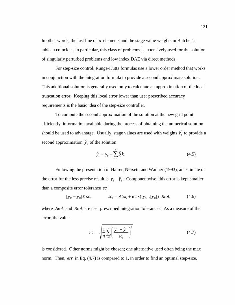
121
In other words, the last line of a elements and the stage value weights in Butcher’s
tableau coincide. In particular, this class of problems is extensively used for the solution
of singularly perturbed problems and low index DAE via direct methods.
For step-size control, Runge-Kutta formulas use a lower order method that works
in conjunction with the integration formula to provide a second approximate solution.
This additional solution is generally used only to calculate an approximation of the local
truncation error. Keeping this local error lower than user prescribed accuracy
requirements is the basic idea of the step-size controller.
To compute the second approximation of the solution at the new grid point
efficiently, information available during the process of obtaining the numerical solution
should be used to advantage. Usually, stage values are used with weights $bi to provide a
second approximation $y1 of the solution
$ $y y b ki ii
s
1 01
= +=
Í (4.5)
Following the presentation of Hairer, Nørsett, and Wanner (1993), an estimate of
the error for the less precise result is y y1 1- $ . Componentwise, this error is kept smaller
than a composite error tolerance sci
| $ | max(| |,| |)y y sc sc Atol y y Rtoli i i i i i i i1 1 0 1- � = + ¿ (4.6)
where Atoli and Rtoli are user prescribed integration tolerances. As a measure of the
error, the value
errn
y y
sci i
ii
n
= -���
���
=
Í1 1 1
2
1
$(4.7)
is considered. Other norms might be chosen; one alternative used often being the max
norm. Then, err in Eq. (4.7) is compared to 1, in order to find an optimal step-size.

122
From asymptotical error behavior, err C hq£ ¿ +1 , and from 1 1£ ¿ +C hoptq (where
q p p= min( , $) , with p and $p being the order of the formulas used), the optimal step size
is obtained as
h herropt
q= ¿���
���
+11
1(4.8)
A safety factor fac usually multiplies hopt such that the error is acceptable at the
end of the next step with high probability. Further, h is not allowed to increase or
decrease too fast. Thus, the value used for the new step-size is
h h fac errnewq= ¿ ¿ +min( , max( , ( ) ))( )facmax facmin 1 1 1
and if at the end of the current step, err � 1, the step is accepted. The solution is then
advanced with y1 and a new step is tried, with hnew as step-size. Otherwise, the step is
rejected and computations for the current step are repeated with the new step-size hnew .
The maximal step-size increase facmax , usually chosen between 1.5 and 5, prevents the
code from taking too large a step and contributes to its safety. When chosen too small, it
may also unnecessarily increase the computational work. Finally, it is advisable to put
facmax = 1 in steps after a step-rejection (Shampine and Watts, 1979).
The last important aspect, from a practical standpoint, is a dense output capability.
This capability is important for many practical questions such as event location and
treatment of discontinuities in differential equations, graphical output, etc. From a
mathematical perspective, this issue is important if the number of output points is very
large. Cutting the step-size, to meet output request and not accuracy or stability
limitations, may reduce efficiency of the algorithm significantly.
These are considerations that motivate the construction of dense output formulas
(Horn, 1983). The idea is to provide, in addition to the numerical result y1 , cheap

123
numerical approximations to y x h( )0 + θ , for the entire integration interval 0 1� �θ .
Thus, using stage values ki , a set of coefficients depending on the output point through
θ , are provided to give an approximation of the solution at the intermediate point
x h0 + θ . This approximate solution is then obtained as
u y h b ki ii
s
( ) ( )θ θ= +=
Í01
(4.9)
where bi ( )θ are polynomials in θ . Based on order conditions, they are determined such
that
u y x h h p( ) ( ) ( )θ θ- + = +
01Ο
where y x( ) is the solution of the IVP and p is the order of the method.
A Runge-Kutta method provided with a formula such as Eq. (4.9) is called a
continuous Runge-Kutta method. The two SDIRK methods presented in this document
for implicit integration of SSODE are continuous methods. Further information
regarding continuous methods can be found in the works of Hairer, Nørsett, and Wanner
(1993) and Shampine (1986).
4.2.2 SDIRK4/16
Since there is no extra price for using a stiffly-accurate Runge-Kutta formula that
can successfully handle even very stiff ODE, this class of integrators was embedded in
the Descriptor Form Method. The Runge-Kutta method implemented was a 5 stage,
order 4, stiffly accurate formula, with error control based on an order 3 embedded
formula. With γ being the diagonal element of the SDIRK formula, define
p1 1= - γ p221 2 2= - +γ γ
p32 31 3 2 3= - + -γ γ γ p4
2 31 6 3 2 3= - + -γ γ γ

124
p52 3 41 4 2 9 2 4= - + - +γ γ γ γ p6
2 3 41 8 4 3 4 4= - + - +γ γ γ γ
p72 3 41 12 7 2 4= - + - +γ γ γ γ p8
2 3 41 24 2 3 3 4= - + - +γ γ γ γ
The following simplified conditions assure the order four of the method (Hairer
and Wanner (1996))
(4.10)
b b b b p1 2 3 4 1+ + + =
b c b c b c p2 2 3 3 4 4 2� + � + � =
b c b c b c p2 22
3 32
4 42
3� + � + � =
b a c b a c a c p3 32 2 4 42 2 43 3 4� + � + � =( )
b c b c b c p2 23
3 33
4 43
5� + � + � =
b c a c b c a c a c p3 3 32 2 4 4 42 2 43 3 6� � + � � + � =( )
b a c b a c a c p3 32 22
4 42 22
43 32
7� + � + � =( )
b a a c p3 43 32 2 8� =
The coefficients ci , are defined as � ==
-
Íc ai ijj
i
1
1
, i = 1 2 3, , . The associated Butcher’s
tableau is given in Table 12.
Table 12. Butcher’s Tableau for SDIRK Formulas
c1 γ 0 … … 0
c2 a21 γ … … 0
… … … … … …
cs as1 as2 … … γ
b1 b2 … … bs

125
The A-stability property of the method is determined by the choice of γ in this
tableau (Hairer and Wanner, 1996). In order to obtain good stability properties, along
with a small leading coefficient of the local truncation, Hairer and Wanner (1996) suggest
values of γ in the range 0.25 and 0.29. For the Descriptor Form Method, the value
chosen was γ = 0 25. (or γ = 4 16 , the name of this formula). According to Butcher’s
tableau, if the number of stages is s = 5 , there are 11 coefficients to be determined,
namely the sub-diagonal elements aij . Once these coefficients are known, since the
method is stiffly stable, the coefficients bi are known. Finally, the coefficients ci are
obtained using the conditions
c ai iji
i
==
Í1
, i = 1 5, ,K
With the coefficient γ chosen, eight order conditions are available in Eq. (4.10)
to compute 11 unknowns. The order of the method and its stability properties are
satisfied by the conditions imposed. Therefore, the two extra degrees of freedom in the
choice of coefficients are used to minimize the fifth-order error terms. This is expected
to attain additional accuracy for the otherwise fourth order formula. This condition leads
to the recommendation that � =c2 05. and � =c3 0 3. (Hairer and Wanner, 1996). With these
two conditions, a non-linear system is solved for aij , and the resulting stiffly-accurate, L-
stable, 5 stage, order 4, Runge-Kutta formula obtained is shown in Table 13.
Step size control is based on an order 3 embedded formula. To obtain the
coefficients of the second formula, order conditions are revisited. They are reformulated
in general form, to obtain a set of equations for the new weights $bi . Since the same stage
values are used, the aij and ci coefficients remain the same. Only the weights that are to
change to produce a new approximation of the solution. The order three conditions
assume the form

126
$bjjÍ = 1
$
$
,
, ,
b a
b a a
j jkj k
j jk jlj k l
Í
Í
=
=
1
2
1
3
(4.11)
$
, ,
b a aj jk klj k lÍ = 1
6
Table 13. SDIRK4/16 Formula for Descriptor Form Method
1/4 1/4 0 0 0 0
3/4 1/2 1/4 0 0 0
11/20 17/50 -1/25 1/4 0 0
1/2 371/1360 -137/2720 15/544 1/4 0
1 25/24 -49/48 125/16 -85/12 1/4
y1 = 25/24 -49/48 125/16 -85/12 1/4
$y1 = 59/48 -17/96 225/32 -85/12 0
Using values of aij from Table 13, these equations lead to the following linear
system for the weights $bi :
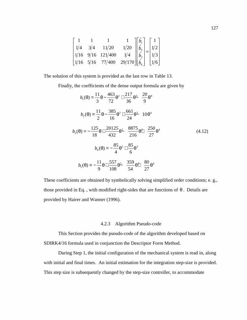
127
1 1 1 1
1 4 3 4 11 20 1 20
1 16 9 16 121 400 1 4
1 16 5 16 77 400 29 170
1
1 2
1 3
1 6
1
2
3
4
�
!
"
$
####
�
!
"
$
#####=
�
!
"
$
####
$
$
$
$
b
b
b
b
The solution of this system is provided as the last row in Table 13.
Finally, the coefficients of the dense output formula are given by
b12 3 411
3
463
72
217
36
20
9( )θ θ θ θ θ= − + −
b22 3 411
2
385
16
661
2410( )θ θ θ θ θ= − + −
b32 3 4125
18
20125
432
8875
216
250
27( )θ θ θ θ θ= − + − + (4.12)
b42 385
4
85
6( )θ θ θ= − +
b52 3 411
9
557
108
359
54
80
27( )θ θ θ θ θ= − + − +
These coefficients are obtained by symbolically solving simplified order conditions; e. g.,
those provided in Eq. , with modified right-sides that are functions of θ . Details are
provided by Hairer and Wanner (1996).
4.2.3 Algorithm Pseudo-code
This Section provides the pseudo-code of the algorithm developed based on
SDIRK4/16 formula used in conjunction the Descriptor Form Method.
During Step 1, the initial configuration of the mechanical system is read in, along
with initial and final times. An initial estimation for the integration step-size is provided.
This step size is subsequently changed by the step-size controller, to accommodate
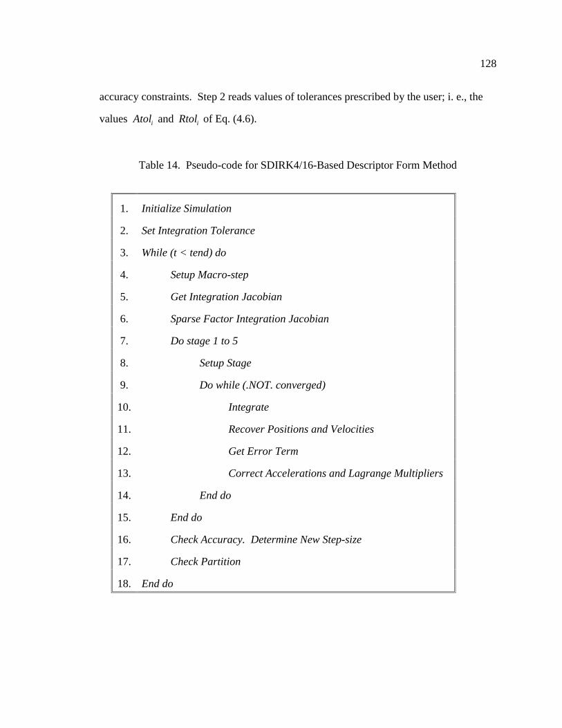
128
accuracy constraints. Step 2 reads values of tolerances prescribed by the user; i. e., the
values Atoli and Rtoli of Eq. (4.6).
Table 14. Pseudo-code for SDIRK4/16-Based Descriptor Form Method
1. Initialize Simulation
2. Set Integration Tolerance
3. While (t < tend) do
4. Setup Macro-step
5. Get Integration Jacobian
6. Sparse Factor Integration Jacobian
7. Do stage 1 to 5
8. Setup Stage
9. Do while (.NOT. converged)
10. Integrate
11. Recover Positions and Velocities
12. Get Error Term
13. Correct Accelerations and Lagrange Multipliers
14. End do
15. End do
16. Check Accuracy. Determine New Step-size
17. Check Partition
18. End do

129
At Step 3 the simulation loop is started, and the code proceeds by setting the new
macro-step. If the step is successful, the current configuration is saved. Otherwise, when
rejected, the initial settings are used again to restart the integration, with step-size
suggested by the step-size controller.
Step 5 is the pivotal point of the implementation. If the current time step has not
been rejected, the integration Jacobian is computed according to considerations of
Section 3.3, which is the CPU intensive part of the code. Otherwise, if the current call to
the integration Jacobian computation comes after an unsuccessful time step, the
integration Jacobian is known, since it assumes the form M M M1 22
3+ +γ βh h , and
matrices M1 , M2 , and M3 are available from the first rejected attempt. Only the step-
size h is modified, and re-computing the integration Jacobian is cheap.
Harwell sparse linear algebra routines are used for factorization of the integration
Jacobian. Since the sparsity pattern of the integration Jacobian does not change during
integration, the factorization process is cheap, once the routine ma48ad of Harwell has
analyzed its structure and a factorization sequence has been determined. All subsequent
calls to integration Jacobian factorization use the much faster ma48bd factorization
routine. Care should be taken to make sure the defining call to ma48ad is done with the
typical sparsity pattern of integration Jacobian, and sometimes this might not be induced
by the first configuration of the mechanism.
At Step 7 is started to loop for the stage values ki . Values iterated for are the
generalized accelerations and Lagrange multipliers. At Step 8, starting values for these
quantities are provided, and the iteration counter is reset to zero. If during a stage of the
formula, this counter exceeds a limit value, the time step is deemed rejected, the
integration step-size is decreased, and the code proceeds to Step 4.

130
The solution of the discretized non-linear algebraic equations is obtained during
the loop that starts at Step 9 and ends at Step 14. As described in Section 3.3.2, based on
the SDIRK formula of Table 13, accelerations are integrated to obtain generalized
velocities, which are integrated to obtain generalized positions. After direct integration
of all generalized accelerations and velocities, the generalized positions and velocities fail
to satisfy the kinematic constraint equations at position and velocity levels. Dependent
positions obtained after direct integration are considered only as starting estimates for
recovering the consistent configuration of the mechanism, via solution of position
kinematic constraint equations. The same observations apply for dependent velocities,
which are computed using velocity kinematic constraint equations. This is the reason for
which, although the discretization is done at the index 1 DAE level, the Descriptor Form
is truly a state-space method.
At Step 13, the error term in satisfying the index 1 DAE is evaluated. At step 14,
corrections in generalized accelerations and Lagrange multipliers are computed. Based
on the norm of these corrections, the integration tolerance, and the norm of the error in
the discretized index 1 DAE, an iteration stopping decision is made. If stopping criteria
are met, the code proceeds to Step 16, once all five stages of the SDIRK4/16 formula
have been completed. Otherwise, corrections in accelerations and Lagrange multipliers
are made, and if the limit number of iterations has not been reached, another iteration is
started.
During Step 16, the step size controller described in Section 4.2.1, based on an
embedded formula provided in the last row of Table 13, analyzes the accuracy of the
numerical solution. If accuracy of the approximate solution is satisfactory, the
configuration at this grid point is accepted, and integration proceeds with a step-size that
is obtained as a by-product of the accuracy check. Otherwise, with the newly computed

131
step-size, the code proceeds to Step 4 to restart integration, this time on the premise of a
rejected time step.
During Step 17, the partitioning of the vector of generalized coordinates is
checked. If necessary, a new dependent/independent partitioning is determined. This
process is detailed for the trapezoidal-based State-Space Method in Section 4.1.2.
Finally, Step 18 is the end of the simulation loop.
4.3 Trapezoidal-Based Descriptor Form
Implicit Integration
The same trapezoidal integration formula used in the framework of the State-
Space Method is used here in conjunction with the Descriptor Form Method.
Characteristics of this integrator, such as stability properties, order, etc. were presented in
Section 4.1.1. Pseudo-code for trapezoidal-based implicit integration of DAE via the
Descriptor Form Method is presented below.
4.3.1 Algorithm Pseudo-code
A large part of the discussion of Section 4.2.2 regarding SDIRK4/16-based
integration via the Descriptor Form Method applies here. Since the discretization is
based on the trapezoidal rather than SDIRK4/16 formula, the numerical implementation
is identical, with the exception that instead of having 5 stages, there is only one stage that
advances the simulation. The pseudo-code of the algorithm is provided in Table 15.
During Stage 4, the system configuration at the beginning of the time step is
saved. This information is used after a rejected time step for reinitializing the state of the
system and restarting integration with a new step-size. Compared to the pseudo-code for

132
SDIRK4/16, the Setup Stage and the loop after the 5 stages do not appear. All other steps
of the implementation are as discussed in Section 4.2.3., in conjunction with the
SDIRK4/16 algorithm. Additional information about this algorithm is provided in the
work of Haug, Negrut, and Engstler (1998).
Table 15. Pseudo-code for Trapezoidal-Based Descriptor Form Method
1. Initialize Simulation
2. Set Integration Tolerance
3. While (t < tend) do
4. Setup Step
5. Get Integration Jacobian
6. Sparse Factor Integration Jacobian
7. Do while (.NOT. converged)
8. Integrate
9. Recover Positions and Velocities
10. Get Error Term
11. Correct Accelerations and Lagrange Multipliers
12. End do
13. Check Accuracy. Determine New Step-size
14. Check Partition
15. End do

133
4.4 Rosenbrock-Based First Order Implicit Integration
4.4.1 General Considerations
The fundamental idea of the proposed algorithm is to reduce the second order
SSODE to an equivalent first order ODE, and apply a Rosenbrock formula to integrate
the ODE. The discussion starts with a brief description of Rosenbrock methods, followed
by a more detailed presentation of how this class of methods is used to integrate the
SSODE of Multibody Dynamics. Finally, a four stage, order 4, L-stable Rosenbrock
method is derived (Sandu, et al., 1998).
For the differential equation
′ =y f y( ) (4.13)
an s stage diagonal implicit Runge-Kutta method defined by the set of coefficients
( , )a bij i assumes the form
k f y k ki ij j ii ij
s
h a a i s= + + ==
−
∑( ) , , ,01
1
1 K (4.14)
y y k1 01
= +=∑bi ii
s
(4.15)
At stage i , the system of nonlinear equations of Eq. (4.14) is solved for k i . The solution
is obtained as a linear combination of stage values k i as indicated in Eq. (4.15).
For Rosenbrock methods, instead of solving a non-linear system at each stage, the
term f ( )⋅ in the right side of Eq. (4.14) is linearized in terms of k i . The stage value k i
is then obtained as the solution of a linear system of equations. The benefit of
Rosenbrock methods lies in this approach to finding k i . It can be shown (Hairer and
Wanner, 1996) that a Rosenbrock method can be interpreted as the application of one

134
Newton iteration to each stage in Eq. (4.14), with starting values k 0i( )0 = . This approach
yields the following method:
k f g f g k
g y k
i i i ii i
i ij jj
i
h h a
a
= + ′
≡ +=
−
∑
( ) ( )
01
1 (4.16)
To gain even more computational advantage, the Jacobian term ′f g( )i in Eq.
(4.16) is replaced by J f y≡ ′( )0 . To satisfy order conditions more easily, additional
linear combinations of terms Jk i are introduced into Eq. (4.16) (Nørsett and Wolfbrandt
1979, Kaps and Rentrop 1979), to arrive at the following class of methods.
Definition 4.1. An s -stage Rosenbrock method is given by the formulas
k f y k J k
y y k
i ij j jjj
i
i ii
s
h a h i s
b
= + + =
= +
==
−
=
∑∑
∑
( ) , , ,011
1
1 01
1eij
i
K
(4.17)
where aij , eij , and bi are the defining coefficients and J f y= ′( )0 .
Each stage of this method consists of a system of linear equations, with unknowns
k i and coefficient matrix I J− heii . Of special interest are methods with
e e ess11 = = =L , for which only one LU decomposition is needed per step.
The case of non-autonomous ordinary differential equations
′ =y f y( , )t (4.18)
is converted to autonomous form by appending to the original ODE the differential
equation ′ =t 1 , and regarding time as one of the variables. In this case, if the method of
Eq. (4.17) is applied, the corresponding Rosenbrock method is obtained as

135
k f y k f y f y k
y y k
yi i ij jj
i
i t ij jj
i
i ii
s
h t a h a e h t h t e
b
= + + + +
= +
=
−
=
=
∑ ∑
∑
( , ) ( , ) ( , )0 01
12
0 0 0 01
1 01
(4.19)
where the additional coefficients are given by
a a e ei ijj
i
i ijj
i
= ==
−
=∑ ∑
1
1
1
, (4.20)
and the notation f ft t≡ ∂ ∂ , and f f yy ≡ ∂ ∂ has been used.
4.4.2 Rosenbrock-Nystrom Methods
Assume in what follows that a second order scalar ordinary differential equation
is given in the form
′′ = ′y f t y y( , , ) (4.21)
The assumption that the differential equation in Eq. (4.21) is scalar simplifies notation
and makes the presentation more accessible. The implications of the case in which y is a
vector will be pointed out when necessary. Technically, they amount to substituting
certain matrix-matrix, and matrix-vector products with tensorial products.
The goal is to apply the formula of Eq. (4.19) to the differential equation in Eq.
(4.21). This is the scenario when the SSODE obtained after DAE-to-ODE reduction is
integrated numerically.
First, the second order ODE is reduced to the first order ODE
y
y
y
f t y y′�!
"$#′
=′
′�!
"$#( , , )
(4.22)
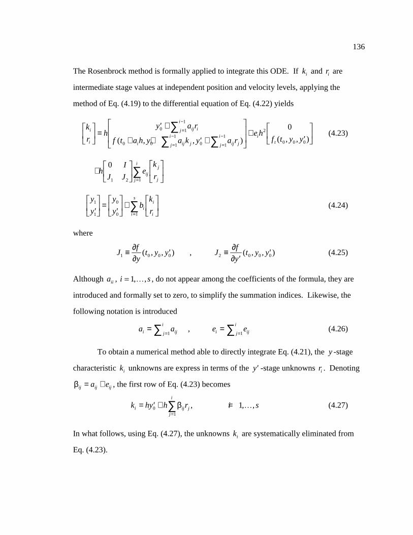
136
The Rosenbrock method is formally applied to integrate this ODE. If ki and ri are
intermediate stage values at independent position and velocity levels, applying the
method of Eq. (4.19) to the differential equation of Eq. (4.22) yields
k
rh
y a r
f t a h y a k y a re h
f t y yi
i
ij ij
i
i ij jj
i
ij jj
i it
�!
"$# =
′ +
+ + ′ +
�
!
"
$## +
′�!
"$#
=
−
=
−
=
−∑
∑ ∑0 1
1
0 0 1
1
0 1
12
0 0 0
0
( , , ) ( , , )(4.23)
+�!
"$#
�!
"$#=
∑hI
J Je
k
rij
j
jj
i0
1 2 1
y
y
y
yb
k
rii
ii
s1
1
0
0 1′�!
"$# =
′�!
"$# +
�!
"$#=
∑ (4.24)
where
Jf
yt y y J
f
yt y y1 0 0 0 2 0 0 0≡ ∂
∂′ ≡ ∂
∂ ′′( , , ) , ( , , ) (4.25)
Although aii , i s= 1, ,K , do not appear among the coefficients of the formula, they are
introduced and formally set to zero, to simplify the summation indices. Likewise, the
following notation is introduced
a a e ei ijj
i
i ijj
i= == =∑ ∑1 1
, (4.26)
To obtain a numerical method able to directly integrate Eq. (4.21), the y -stage
characteristic ki unknowns are express in terms of the ′y -stage unknowns ri . Denoting
βij ij ija e= + , the first row of Eq. (4.23) becomes
k hy h r i si ij jj
i
= ′ + ==
∑01
1β , , ,K (4.27)
In what follows, using Eq. (4.27), the unknowns ki are systematically eliminated from
Eq. (4.23).

137
The term a kij jj
i
=
−∑ 1
1 appears as the second argument of f ( , , )⋅ ⋅ ⋅ . Using Eq. (4.27),
and interchanging the order of summation, this term is expressed as
a k a hy r ha y a r
ha y a r a r a r ha y r
ij jj
i
ij jm mm
j
j
i
i ij jm mm
j
j
i
i ij jj
i
ij jj
i
ij j i ij i
i
i ij mj
i
=
−
==
−
==
−
=
−
=
−
− −= −
−
=
−
∑ ∑∑ ∑∑
∑ ∑ ∑ ∑
= ′ +���
��� = ′ +
���
���
= ′ + + +���
��� = ′ +
1
1
011
1
011
1
0 1 11
1
2 22
1
1 11
1
01
1
β β
β β β δK ,
where
µ βij im mjm j
i
a==
-
Í1
(4.28)
Since this procedure of expressing ki in terms of ri will to appear several times
during this discussion, a matrix representation that simplifies the process is introduced. If
k ≡ [ , , , ]k k ks1 2 K T , and r ≡ [ , , , ]r r rs1 2 K T , based on Eq. (4.27),
k 1 Br= ′ ⋅ +hy h0 (4.29)
where the vector 1 ∈ℜs is defined as 1 ≡ [ , , , ]11 1K T , and
B B≡ ∈ℜ ×( ),βijs s (4.30)
For stage i s= 1, ,K , terms such as a kij jj
i
=
−∑ 1
1 can be simultaneously evaluated by using
the matrix notation introduced. In this notation, using Eq. (4.29), the array z ∈ℜs ,
z ≡=
−∑ a kij jj
i
i1
14 9 , can be expressed as
z Ak A 1 Br ABr r= = ′ ⋅ + = ′�
!
"
$###
+ = ′ +( ) ( )hy h hy
a
a
h hy a h
s
i0 0
1
0M ∆
where, if multiplication is carried out to compute the matrix ∆ ≡ AB , it can be seen that
∆ µ= ( )ij , with µij given by Eq. (4.28).
The second row of Eq. (4.23) can now be expressed as

138
r hf t a h y ha y h r y a r
e hf
tt y y hJ e k hJ e r
i i i ij jj
i
ij jj
i
i ij jj
i
ij jj
i
= + + � + � +
+ ��
� + +
=
-
=
-
= =
Í Í
Í Í
( , , )
( , , )
0 0 01
1
01
1
20 0 0 1
12
1
δ(4.31)
In order to eliminate the k j that multiply J1 in Eq. (4.31), the matrix notation and the
notation in Eq. (4.26) are used to yield
e k hy h hy e e h
hy e h
ij jj
i
i
s
i s
=∑
���
��� = = ′ ⋅ + = ′ +
≡ ′ +1
0 0 1
0
Ek E 1 Br EBr
Q
( )
( )
LT
where Q EB= ≡( )qij . Stage i finally assumes the form
r hf t a h y ha y h r y a r
e hf
tt y y J y h J q r hJ e r
i i i ij jj
i
ij jj
i
i ij jj
i
ij jj
i
= + + ′ + ′ +
+ ∂∂
′ + ′���
��� + +
=
−
=
−
= =
∑ ∑
∑ ∑
( , , )
( , , )
0 0 01
1
01
1
20 0 0 1 0
21
12
1
δ(4.32)
Since q e e e a e eii ii ii ii ii ii ii= = + = =β ( ) 2 2 , at stage i , 1 ≤ ≤i s , ri is computed as the solution
of the linear system
Sr hf t a h y ha y h r y a r
e hf
tt y y J y h J q r hJ e r
i i i ij jj
i
ij jj
i
i ij jj
i
ij jj
i
= + + ′ + ′ +
+ ∂∂
′ + ′���
��� + +
=
−
=
−
=
−
=
−
∑ ∑
∑ ∑
( , , )
( , , )
0 0 01
1
01
1
20 0 0 1 0
21
1
1
21
1
δ(4.33)
S ≡ − −I heJ h e J22 2
1 (4.34)
Due to the choice of coefficients e e ess11 = = =K , only one matrix factorization
needs to be computed per successful time step. At each stage, this factorization is used to
compute ri . Note that the right side of Eq. (4.33) depends on past information only.
Once ri . i s= 1, ,K , are available, the solution is obtained from Eq. (4.24) via Eq. (4.27).

139
In matrix notation, if b is the row vector b = [ , , ]b bs1 K , the solution at the velocity level
is given by
′ = ′ +y y1 0 br (4.35)
Taking into account Eq. (4.29) and the fact that for Runge-Kutta methods
b bs1 1+ + =K , the solution at the position level is obtained as
y y hy h1 0 0= + ′ + mr (4.36)
where the row vector m is defined as
m bB= (4.37)
To summarize, the following linearly implicit method for solution of the second
order ODE of Eq. (4.21) has been defined:
Y y ha y h ri i ij jj
i
= + � +=
-
Í0 01
1
µ (4.38)
′= ′ +=
−
∑Y y a ri ij jj
i
01
1
(4.39)
Sr hf t a h Y Y e hf
tt y y J y
h J q r hJ e r
i i i i i
ij jj
i
ij jj
i
= + ′ + ∂∂
′ + ′���
���
+ +=
−
=
−
∑ ∑
( , , ) ( , , )02
0 0 0 1 0
21
1
1
21
1(4.40)
y y hy h m ri ii
s
1 0 01
= + ′ +=∑ (4.41)
′ = ′ +=∑y y h b ri ii
s
1 01
(4.42)
Following a remark of Hairer and Wanner (1996), when implementing the
Rosenbrock method of Eqs. (4.38) through (4.42), one matrix-vector multiplication can
be saved. For this, a new set of unknowns is introduced as
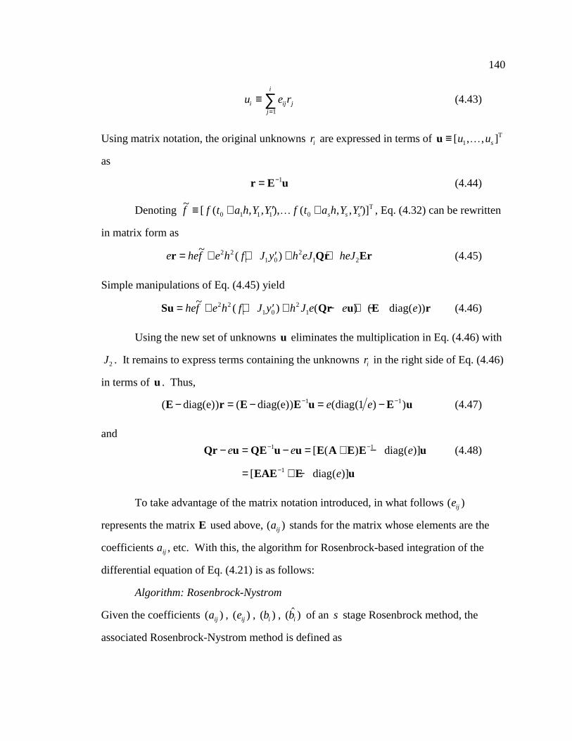
140
u e ri ij jj
i
≡=
∑1
(4.43)
Using matrix notation, the original unknowns ri are expressed in terms of u ≡ [ , , ]u us1 KT
as
r E u= −1 (4.44)
Denoting ~
[ ( , , ), ( , , )]f f t a h Y Y f t a h Y Ys s s≡ + ′ + ′0 1 1 1 0K T , Eq. (4.32) can be rewritten
in matrix form as
e hef e h f J y h eJ heJtr Qr Er= + + ′ + +~( )2 2
1 02
1 2 (4.45)
Simple manipulations of Eq. (4.45) yield
Su Qr u E r= + + ′ + − + −hef e h f J y h J e e et
~( ) ( ) ( ( ))2 2
1 02
1 diag (4.46)
Using the new set of unknowns u eliminates the multiplication in Eq. (4.46) with
J2 . It remains to express terms containing the unknowns ri in the right side of Eq. (4.46)
in terms of u . Thus,
( ) ( ) ( ( ) )E r E E u E u− = − = −− −diag(e) diag(e) diag1 11e e (4.47)
and
Qr u QE u u E A E E u− = − = + −− −e e e1 1[ ( ) ( )]diag (4.48)
= + −−[ ( )]EAE E u1 diag e
To take advantage of the matrix notation introduced, in what follows ( )eij
represents the matrix E used above, ( )aij stands for the matrix whose elements are the
coefficients aij , etc. With this, the algorithm for Rosenbrock-based integration of the
differential equation of Eq. (4.21) is as follows:
Algorithm: Rosenbrock-Nystrom
Given the coefficients ( )aij , ( )eij , ( )bi , ( $ )bi of an s stage Rosenbrock method, the
associated Rosenbrock-Nystrom method is defined as

141
y y hy h p ui ii
s
1 0 01
= + ′ +=∑ , $ $y y hy h p ui i
i
s
1 0 01
= + ′ +=∑ (4.49)
′ = ′ +=∑y y s ui ii
s
1 01
, ′ = ′ +=∑$ $y y s ui ii
s
1 01
(4.50)
Y y ha y h t ui i ij jj
i
= + ′ +=
−
∑0 01
1
(4.51)
�= � +=
-
ÍY y w ui ij jj
i
01
1
(4.52)
Su hef t a h Y Y h eef
tt y y J y
e c u h eJ d u
i i i i i
ij jj
i
ij jj
i
= + ′ + ∂∂
′ + ′���
���
+ +=
−
=
−
∑ ∑
( , , ) ( , , )02
0 0 0 1 0
1
12
11
1(4.53)
where
( ) ( )( )
( ) ) ( )
( ) ( ) ( )( )( )
( ) ( ) ( ) ( )
( ) ( )( )
( $ ) ( )( )
( ) ( ) ( )( )( )
( $ ) ( $ ) ( $ )( )( )
( ) ( )
( ) ( )
w a e
c e
d e e a e
t a a e
s b e
s b e
p b b a e
p b b a e
e e
a a
ij ij ij
ij ij
ij ij ij ij ij
ij ij ij ij
i i ij
i i ij
i i i ij ij
i i i ij ij
i ij
i ij
=
= −
= +
= +
=
=
= +
= += ⋅
= ⋅
−
−
−
−
−
−
−
−
1
1
1
2 1
1
1
1
1
diag(1 e
1
1
(4.54)
The matrices of coefficients ( )aij , ( )eij , and ( )bi define the Rosenbrock-Nystrom
algorithm, including order and stability properties. All other coefficients of the algorithm
are derived based on these coefficients.

142
Depending on the application that is numerically integrated, different orders and
stability requirements should be considered. For the specific class of Multibody
Dynamics problems, a low-to-medium accuracy method with good stability properties is
desirable. Formulas with few function evaluations are favored, since function
evaluations for mechanical system simulation amount to acceleration evaluations, which
are expensive.
A method that is L stable allows for robust integration of very stiff problems.
Consequently, bushing elements and flexible components used in modeling mechanical
systems can be efficiently handled. An order 4 formula should reliably meet all accuracy
requirements likely be considered for Multibody Dynamics simulation. With these
considerations in mind, the defining matrices of coefficients ( )aij , ( )eij , and ( )bi are
selected such that the resulting Rosenbrock-Nystrom method is of order 4 and is L stable.
The number of stages of the method is chosen to be 4. This leaves some freedom in the
choice of the embedded method for step-size control. Following an idea suggested by
Hairer and Wanner (1996), the number of function evaluations is kept to 3; i.e., one
function evaluation is saved. This makes the Rosenbrock-Nystrom method competitive
with the trapezoidal method whenever the latter method requires 3 or more iterations for
convergence. However, the proposed method is L stable while the trapezoidal method is
not. Furthermore, the difference in order is 2: 4 for Rosenbrock-Nystrom, and 2 for
trapezoidal.
4.4.3 Order Conditions For Rosenbrock-Nystrom
Algorithm
The order conditions refer to conditions the defining coefficients ( )aij , ( )eij , and
( )bi should satisfy such that the method has a certain order. The discussion here is based

143
on results presented by Hairer and Wanner (1996). In order to construct an order 4
Rosenbrock method, the order conditions are as follows:
b b b b1 2 3 4 1+ + + = (4.55)
b b b e2 2 3 3 4 4 1 2′ + ′ + ′ = −β β β (4.56)
b a b a b a2 22
3 32
4 42 1 3+ + = (4.57)
b b e e3 32 2 4 42 2 43 321 6β β β β β β′ + ′ + ′ = − +( ) (4.58)
b a b a b a2 23
3 33
4 43 1 4+ + = (4.59)
b a a b a a ae
3 3 32 2 4 4 42 2 43 3
1
8 3′ + ′ + ′ = −β β β( ) (4.60)
b a b a a e3 32 22
4 42 22
43 32 1 12 3β β β+ + = −( ) (4.61)
be
e e4 43 32 22 31 24
2
3
2β β β′ = − + − (4.62)
where the following abbreviations are used
a ai ijj
i
i ijj
i
= ′ ==
−
=
−
∑ ∑1
1
1
1
, β β
The step size control mechanism is based on an embedded formula (Kaps and
Rentrop, 1979) of the form
$ $y y b kj jj
s
1 01
= +=
∑
which uses the stage values ki from Eqs. (4.19). The embedded method should be of
order 3; i. e., the order conditions of Eqs. (4.55) through (4.57) must be satisfied. These
conditions lead to the system
1 1 1 1
0
0
0 0
1
1 2
1 3
1 6
2 3 4
22
32
42
32 2 42 2 43 3
1
2
3
42
′ ′ ′
′ ′ + ′
�
�
����
�
�
����
�
�
����
�
�
����=
−
− +
�
�
����
�
�
����β β β
β β β β β βa a a
b
b
b
b
e
e e
$
$
$
$
(4.63)
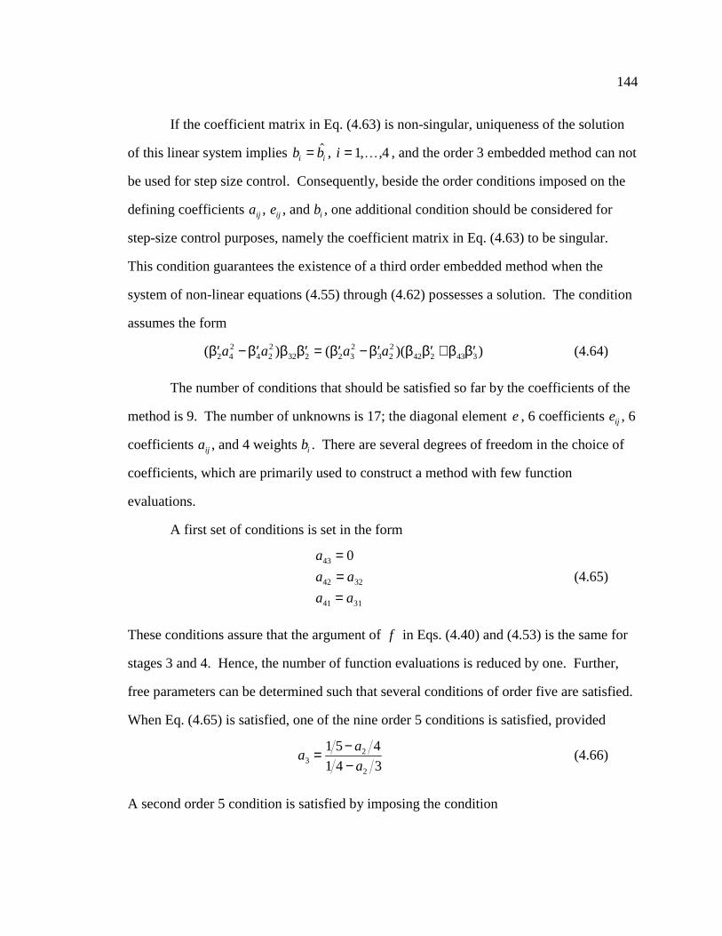
144
If the coefficient matrix in Eq. (4.63) is non-singular, uniqueness of the solution
of this linear system implies b bi i= $ , i = 1 4, ,K , and the order 3 embedded method can not
be used for step size control. Consequently, beside the order conditions imposed on the
defining coefficients aij , eij , and bi , one additional condition should be considered for
step-size control purposes, namely the coefficient matrix in Eq. (4.63) to be singular.
This condition guarantees the existence of a third order embedded method when the
system of non-linear equations (4.55) through (4.62) possesses a solution. The condition
assumes the form
( ) ( )( )′ − ′ ′ = ′ − ′ ′ + ′β β β β β β β β β β2 42
4 22
32 2 2 32
3 22
42 2 43 3a a a a (4.64)
The number of conditions that should be satisfied so far by the coefficients of the
method is 9. The number of unknowns is 17; the diagonal element e , 6 coefficients eij , 6
coefficients aij , and 4 weights bi . There are several degrees of freedom in the choice of
coefficients, which are primarily used to construct a method with few function
evaluations.
A first set of conditions is set in the form
a
a a
a a
43
42 32
41 31
0===
(4.65)
These conditions assure that the argument of f in Eqs. (4.40) and (4.53) is the same for
stages 3 and 4. Hence, the number of function evaluations is reduced by one. Further,
free parameters can be determined such that several conditions of order five are satisfied.
When Eq. (4.65) is satisfied, one of the nine order 5 conditions is satisfied, provided
aa
a32
2
1 5 4
1 4 3= −
−(4.66)
A second order 5 condition is satisfied by imposing the condition

145
b a a ae
ae
4 43 32
3 2 2
1
20 4
1
12 3β ( )− = − − −�
����� (4.67)
Next, two conditions are chosen as
b
a e3
2
0
2
==
(4.68)
to make the task of finding a solution more tractable. The last condition regards the
choice of the diagonal element e . The value of this parameter determines the stability
properties of the Rosenbrock method. Since interest is in constructing an L-stable
method, the coefficient e should be taken as (Hairer and Wanner, 1996)
e = 057281606. (4.69)
Equations (4.55) through (4.62) and (4.64) through (4.69) comprise a system of
17 non-linear equations in 17 unknowns. The solution of this system is (Sandu, et al.,
1998):
e
e
e
e
e
e
e
== −= −== −= −= −
057281606
2 34199312711201394917052
0 0273337465434898361965046
0 213811650836699689867472
0 259083837785510222112641
0190595807732311751616358
0 228031035973133829477744
21
31
32
41
42
43
.
.
.
.
.
.
.
a
a
a
a
a
a
21
31
32
41
42
43
114563212
0 520920789130629029328516
0134294186842504800149232
0 520920789130629029328516
0134294186842504800149232
=====
.
.
.
.
= 0.0
.
(4.70)

146
b
b
b
b
1
2
3
4
0 324534707891734513474196
0 049086544787523308684633
0 0
0 6263787473207421778411711
====
.
.
.
.
These coefficients define the proposed 4-stage, L-stable, order 4 Rosenbrock-Nystrom
method with 3 function evaluations per successful integration time-step. The weights of
the embedded formula are computed as the solution of the linear system in Eq. (4.63),
$
$ .
$ .
$ .
b
b
b
b
1
2
3
4
0520920789130629029328516
0144549714665364599584681
0124559686414702049774897
0 209969809789304321311906
=
=
=
=
.
(4.71)
In order to save one matrix-vector multiplication, the approach in Eqs. (4.49)
through (4.53) is implemented. The coefficients in this formulation are obtained from the
coefficients of Eqs. (4.70) and (4.71), based on Eq. (4.54). The following are the
coefficients that are actually used in the numerical implementation of the proposed
Rosenbrock-Nystrom method:
w E
w E
w E
w E
w E
w
21
31
32
41
42
43
0 200000000000000000000000 0
0186794814949823713234476 1
0 234445568517238850023220 0
0186794814949823713234476 1
0 234445568517238850023220 0
0 0
======
.
.
.
.
.
.
(4.72)
c E
c E
c E
c E
c E
c E
21
31
32
41
42
43
0 713764994334997983036926 1
0 258092366650965771448805 1
0 651629887302032023387417 0
0 213711526650661911680637 1
0 321469531339951070769241 0
0 694966049282445225157329 0
= -=== -= -= -
.
.
.
.
.
.
(4.73)

147
d E
d E
d E
d E
d E
d E
21
31
32
41
42
43
0119636100711201394917052 1
0147028025440978071463387 1
0 348105837679204490016704 0
0 003765094355556165798974 0
0109762486758103255675398 0
0 228031035973133829477744 0
= -==== -= -
.
.
.
.
.
.
(4.74)
t E
t E
t E
t E
t E
t
21
31
32
41
42
41
0114563212 1
0 789509162815638629626980 0
0134294186842504800149232 0
0 789509162815638629626980 0
0134294186842504800149232 0
0 0
======
.
.
.
.
.
.
(4.75)
s E
s E
s E
s E
1
2
3
4
0 225556622860456524372884 1
0 287055063194157607662630 0
0 435311963379983213402707 0
0109350765640324780321482 1
====
.
.
.
.
(4.76)
ev E
ev E
ev E
ev E
1
2
3
4
0187167068076981509470170 0
0 048373711126624809706137 0
0 071938617944591505140960 0
0 726950528467092658905657 0
====
.
.
.
.
(4.77)
p E
p E
p
p E
1
2
3
4
0159275081940958534207490 1
0195938266310250609693329 0
0 0
0 626378747320742177841171 0
= .
= .
= .
= .
(4.78)
ep E
ep E
ep E
ep E
1
2
3
4
015784684756137586944780 0
0 027040406278447759351824 0
0124559686414702049774897 0
0 416408937531437856529265 0
== -= -=
.
.
.
.
(4.79)

148
e E
e E
e E
e E
1
2
3
4
0572816060 0
0176917706711201394917052 1
0 759293964293209853670967 0
0104894621490955803206743 0
== -== -
.
.
.
.
(4.80)
a E
a E
a E
1
2
3
01145632120 1
0 655214975973133829477748 0
0 655214975973133829477748 0
===
.
.
.
(4.81)
In Eqs. (4.77) and (4.79), instead of providing the value of the weights $si and $pi
for the embedded method, the difference between the weights of the actual and embedded
methods were computed. The coefficients evi and epi , i = 1 4, ,K are used to compute
the composite error at the position and velocity levels, using the stage unknowns ui .
4.4.4 Algorithm Pseudo-code
Pseudo-code for numerical implementation of the Rosenbrock-Nystrom method
presented in the previous two Sections is provided in Table 16. Coding this algorithm
requires implementation of Eqs. (4.49) through (4.53), using coefficients provided in the
previous section.
The first two steps of the implementation are identical to those of the previously
presented pseudo-codes. Step 4 saves the system configuration to be used upon a
rejected time step. During the following two steps, the integration Jacobian is evaluated
and factored. The quantity that is computed is in fact not the matrix S of Eq. (4.34), as
the Rosenbrock formula suggests, but the matrix Π ¢ ¿( ) $1 2e MS , with $M being the
positive definite matrix of Eq. (3.16). Matrix Π is not obtained by first computing the
matrices $M and S , and then multiplying them. As shown in Section 3.4.1.3
(Proposition 1), the matrix Π is identical to the integration Jacobian Ψ&&v of the State

149
Space Method. Compared to matrix S , Ψ&&v is easier to compute. Therefore, at each stage
of the Rosenbrock formula, instead of solving systems of the form
Sx b=
the vector x is obtained as the solution of the equivalent system
Πx Mb= $ (4.82)
Table 16. Pseudo-code for Rosenbrock-Nystrom-Based First Order Reduction Method
1. Initialize Simulation
2. Set Integration Tolerance
3. While (t < tend) do
4. Set Macro-step
5. Get Integration Jacobian
6. Factor Integration Jacobian
7. Get the Time Derivative
8. Resolve Stage 1
9. Resolve Stage 2
10. Resolve Stage 3
11. Resolve Stage 4
12. Get Solution. Check Accuracy. Compute new Step-size
13. Check Partition
14. End do
The matrix Π is factored during Step 6. The dimension of this matrix is equal to
the number of degrees of freedom of the model, and therefore is rather small. During

150
Step 7, the partial derivative � �f t is evaluated in the consistent configuration from the
beginning of each macro-step. In the case of scleronomic mechanical systems, for which
all the external applied forces are time independent, the quantity � �f t is zero.
Otherwise, adequate means to provide this quantity should be embedded in the code.
The next four steps compute the stage variables ui , i = 1 4, ,K . The challenge is
how to retrieve the right side of Eq. (4.53). During each of the four stages, some or all of
the following steps are taken:
(a). Obtain a consistent configuration at position and velocity levels
(b). Compute generalized accelerations
(c). Evaluate right side of Eq. (4.53)
(d). Solve linear system to obtain the stage values ui
Step (a) is justified by the necessity to compute generalized accelerations required
by step (c). Since the fundamental idea in DAE integration hinges upon state-space
reduction, the Rosenbrock formula actually integrates independent variables only.
Dependent variables must be recovered, since any call to acceleration computation
requires consistent position and velocity information. Independent positions are
computed based on Eq. (4.51), while independent velocities are computed at each stage,
as indicated by Eq. (4.52).
After recovering dependent positions and velocities, based on kinematic
constraint equations of Eqs. (3.7) and (3.8), topology based linear algebra algorithms
introduced in Sections 3.4.2 and 3.4.3 are employed to compute accelerations during sub-
step (c). During sub-step d), the available information is used to obtain the right side of
Eq. (4.53). The actual implementation is based on the matrix Π . Therefore, one
additional step is taken to multiply $M of Eq. (3.16) with the original right-side. As

151
shown in Section 3.4.1.3, this approach adds one matrix-vector multiplication, but
eliminates the need to explicitly solve for J1 and J2 .
Due to the particular choice of coefficients defining the Rosenbrock formula and
the way in which the code was implemented, each of the four stages has its own
particularities. Thus,
(1). Stage 1 (Step 8 of the pseudo-code) coincides with the beginning of the current
macro-step, or equivalently the end of the prior macro-step. Therefore, the system
is in an assembled configuration, and sub-step a) is skipped. During this stage, the
matrix Π is evaluated, and generalized accelerations are obtained cheaply as a by-
product of this effort. To obtain Π , the matrix $M is computed, and the dependent
sub-Jacobian Φu is factored. The latter is needed to obtain the matrices H , J , L ,
and N of Section 3.4.1.3. If these two quantities are available, &&v is first computed
as the solution of the positive definite linear system of Eq. (3.15), and &&u is
computed using acceleration kinematic equation of Eq. (3.9), since Φu is already
factored. Consequently, sub-stages (a) and (b) are effectively dealt with by stage 1.
Obtaining the right-side during sub-step (c) is straightforward. Then, the matrix Π
is factored, and the stage value u1 computed. Note that factorization of Π is used
for all stages of the formula, since the diagonal elements in Butcher’s tableau are
identical.
(2). Stages 2 and 3 (Steps 9 and 10) simply follow the sub-stages (a) through (d) above.
(3). Stage 4 by-passes sub-stage (b), the function evaluation, due to the choice of
formula defining coefficients in Eq. (4.65). Since no acceleration computation is
required, there is no need to provide a consistent configuration at the position and
velocity levels. Therefore sub-stage (a) is skipped. It remains to compute the right

152
side of the linear equation and, with the coefficient matrix already factored, to do a
forward/backward substitution to obtain u4 .
Once all the stage values ui , i = 1 4, ,K are available, the solution at the new grid
point is computed during Step 12, based on Eqs. (4.49) and (4.50). Extra effort goes into
recovering dependent positions and velocities to obtain a consistent configuration of the
mechanism, which is used during the next time step, at stage 1, sub-stage (a).
Based on a second approximation of the solution at the new grid point given by
the embedded formula, values $y1 and $ �y1 of Eqs. (4.49) and (4.50), the accuracy of the
solution is analyzed, and the step is accepted or rejected. As a result of error analysis, a
new step-size is provided. This is used to recompute the current time step upon a rejected
step, or to proceed to the next time step upon a successful step.
Finally, the last step of the algorithm checks the partitioning. Based on the
condition number of the dependent sub-Jacobian Φu , which is available on exit from
Step 12, and the value of the repartitioning coefficient α previously introduced, the
partitioning can be rejected or preserved for the next time step.
The most important feature of any Rosenbrock formula is its ability to provide
accuracy and stability without the penalty of having to solve discretized non-linear
algebraic equations. No iterative process is embedded in the formula, and the delicate
issue of stopping criteria is eliminated. It is recognized in the numerical analysis
community that implementation of a Rosenbrock formula is significantly simpler than
any other Runge-Kutta type formula.
The factor that has limited extensive use of the attractive class of Rosenbrock
formulas is the requirement that the integration Jacobian should be exact. This is a
limiting factor for many engineering applications that are likely to contain complex
components for which computing exact Jacobian is an intractable task. In the context of

153
the dynamic analysis of multibody systems, the limiting factor remains the task of
providing force derivatives. In situations such as these, when no close/analytic
expressions are available to compute required derivative information, the solution is
either to use automatic differentiation tools such as ADIFOR (Bischof et al., 1994), or to
use numerical means to obtain derivative information. In the latter case however, using a
Rosenbrock type formula is no longer an option, and the only alternative is to use more
robust and somehow more CPU-expensive methods. One of these methods is the
SDIRK4/15 formula that is discussed in the next Section.
4.5 SDIRK-Based First Order Implicit Integration
4.5.1 SDIRK4/15
According to Hairer and Wanner (1996), the choice γ = 4 15 instead of γ = 4 16
as the diagonal element of a 5 stage, order 4 stiffly-accurate SDIRK method is
numerically superior. This motivated their effort to code this formula, rather than the one
proposed in Section 4.2 in conjunction with the Descriptor Form Method. The resulting
code is much more refined, and special attention was paid to issues such as stopping
criteria, mechanisms for early detection of convergence failure, estimation of iteration
starting points, avoiding rounding errors, etc.
One positive feature of the First Order Reduction Method is its ability to link to
any standard code for the numerical solution of stiff ODE. This feature is exploited here
by embedding a public domain ODE code of Hairer and Wanner in the framework of the
First Order Reduction Method. The objective is to keep as much as possible of the
original layout that made the code of Hairer and Wanner robust and efficient. There is no

154
major difference between the SDIRK formula of this Section, and the one defined in
Section 4.2.2, so the notation of that Section is retained.
Simplified order conditions for SDIRK4/15 are provided in Eq. (4.10), and values
for pi , i = 1 8, ,K , are obtained by setting γ = 4 15 . The SDIRK4/15 formula is chosen
to be stiffly-stable, and the particular choice of γ implies that it is A-stable (Hairer and
Wanner, 1996). Consequently, it is L-stable. As in Section 4.2.2, in order to minimize
fifth-order error terms, the same values � =c2 05. and � =c3 0 3. are considered for the two
extra coefficients defining the integration formula. After solving the non-linear system in
Eq. (4.10), the coefficients of the formula are obtained as
Stage 1 a11 4 15=
Stage 2a
a21
22
1 2
4 15
==
Stage 3
a
a
a
31
32
33
7809 144200
4 15
== -=
51069 144200
Stage 4
a
a
a
a
41
42
43
44 4 15
====
12047244770625658 141474406359725325
-3057890203562191 47158135453241775
2239631894905804 28294881271945065
Stage 5
a
a
a
a
a
51
52
53
54
55 4 15
=====
181513 86430
-89074 116015
83636 34851
-69863904375173 23297141763930
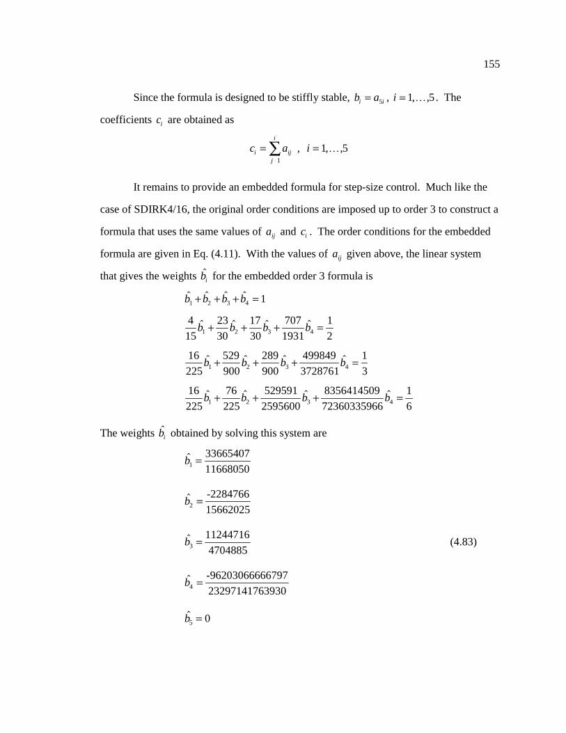
155
Since the formula is designed to be stiffly stable, b ai i= 5 , i = 1 5, ,K . The
coefficients ci are obtained as
c ai ijj
i
==
Í1
, i = 1 5, ,K
It remains to provide an embedded formula for step-size control. Much like the
case of SDIRK4/16, the original order conditions are imposed up to order 3 to construct a
formula that uses the same values of aij and ci . The order conditions for the embedded
formula are given in Eq. (4.11). With the values of aij given above, the linear system
that gives the weights $bi for the embedded order 3 formula is
$ $ $ $b b b b1 2 3 4 1+ + + =
4
15
23
30
17
30
707
1931
1
21 2 3 4$ $ $ $b b b b+ + + =
16
225
529
900
289
900
1
31 2 3 4$ $ $ $b b b b+ + + =499849
3728761
16
225
76
225
1
61 2 3 4$ $ $ $b b b b+ + + =529591
2595600
8356414509
72360335966
The weights $bi obtained by solving this system are
$b1 =33665407
11668050
$b2 =-2284766
15662025
$b3 =11244716
4704885(4.83)
$b4 =-96203066666797
23297141763930
$b5 0=

156
To reduce the influence of round-off errors during numerical integration of the
IVP � =y f x y( , ) , y x y( )0 0= , Hairer and Wanner in their code preferred to work at each
stage with the quantities
z h a f x c h y zi ij j jj
i
= + +=
Í ( , )0 01
, i s= 1, ,K (4.84)
Whenever the solution z1 , z2 ,…, zs of the system in Eq. (4.84) is known, the stage
values ki are obtained as
k f x c h y zi i i= + +( , )0 0
This assumes s -extra function evaluations. The additional effort can be avoided if the
matrix A = ( )aij ; i. e., the matrix of aij coefficients in Butcher’s tableau, is non-singular.
Since this is the case with any SDIRK formula, the system in Eq. (4.84) is rewritten as
z
z
hf x c h y z
hf x c h y zs s s
1 0 1 0 1
0 0
M M
�
���
�
��� =
+ +
+ +
�
���
�
���A
( , )
( , )
(4.85)
The solution at the new grid point is obtained as
y y d zi ii
s
1 01
= +=
Í
where,
( , , ) ( , , )d d b bs s1 11K K= ¿ -A
One attractive feature of the z -approach is that, since SDIRK4/15 is stiffly stable,
the vector d is simply ( , , , , )0 0 0 0 1 . Another advantage of using the z -approach is the
following. The quantities z1 , z2 ,…, zs are computed iteratively and therefore affected by
small iteration errors. The evaluation of ki ; i. e., evaluations of the form
f x c h y zi i( , )0 0+ + would then, due to the large Lipschitz constant of f , amplify these
errors. This could be disastrously inaccurate for a stiff problem (Shampine, 1980).
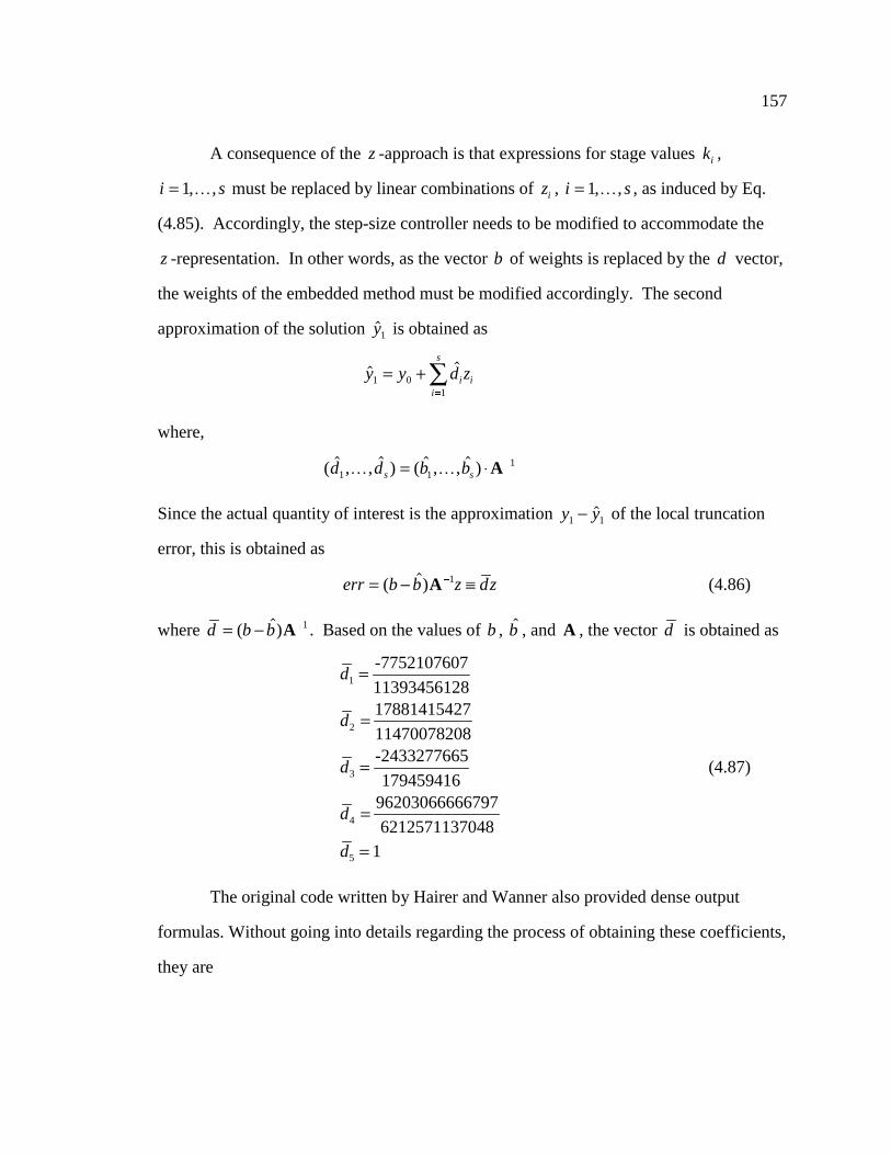
157
A consequence of the z -approach is that expressions for stage values ki ,
i s= 1, ,K must be replaced by linear combinations of zi , i s= 1, ,K , as induced by Eq.
(4.85). Accordingly, the step-size controller needs to be modified to accommodate the
z -representation. In other words, as the vector b of weights is replaced by the d vector,
the weights of the embedded method must be modified accordingly. The second
approximation of the solution $y1 is obtained as
$ $y y d zi ii
s
1 01
= +=
Í
where,
( $ , , $ ) ( $ , , $ )d d b bs s1 11K K= ¿ -A
Since the actual quantity of interest is the approximation y y1 1- $ of the local truncation
error, this is obtained as
err b b z dz= - ¢-( $)A 1 (4.86)
where d b b= - -( $)A 1 . Based on the values of b , $b , and A , the vector d is obtained as
d
d
d
d
d
1
2
3
4
5 1
=
=
=
=
=
-7752107607
1139345612817881415427
11470078208-2433277665
17945941696203066666797
6212571137048
(4.87)
The original code written by Hairer and Wanner also provided dense output
formulas. Without going into details regarding the process of obtaining these coefficients,
they are

158
d
d
11
12
=
==
==
24.74416644927758
-4.325375951824688
d 41.39683763286316
d -61.04144619901784
d -3.391332232917013
13
14
15
d
d
d
d
d
21
22
23
24
25
=
==
==
-51.98245719616925
10.52501981094525
-154.2067922191855
214.3082125319825
14.71166018088679
d
d
d
d
d
31
32
33
34
35
=
==
==
33.14347947522142
-19.72986789558523
230.4878502285804
-287.6629744338197
-18.99932366302254
d
d
d
d
d
41
42
43
44
45
=
==
==
-5.905188728329743
13.53022403646467
-117.6778956422581
134.3962081008550
8.678995715052762
The way in which these coefficients are computed was discussed in Section 4.2.2,
when defining dense output for SDIRK4/16. These coefficients were scaled by A-1 to
account for the zi rather the ki implementation of the formula. For i = 1 5, ,K , with
b di jij
j
( )θ θ==
Í1
4
the solution at an intermediate point x h0 + θ , 0 1< �θ , is given by

159
y x h y b zi ii
( ) ( )0 01
5
+ £ +=
Íθ θ
which is of order 3 for 0 1< <θ , and updates to the fourth order approximation y1 for
θ = 1.
4.5.2 Algorithm Pseudo-code
The SDIRK4/15 formula was embedded in the First Order Reduction Method to
provide a robust and efficient algorithm. The numerical implementation is based on a
public domain code developed by Hairer and Wanner for the integration of stiff IVP,
which was adapted to support the proposed algorithm.
An obstacle to immediate conversion of the algorithm is the need to embed
dependent variable recovery in the original code. Likewise, the SSODE obtained in
Multibody Dynamics is of second order, and the original code was designed for first
order systems with tailored linear algebra, iteration starting values, and stopping criteria.
The pseudo-code of the resulting algorithm is presented in Table 17.
The first four steps of the implementation are the same as discussed in Section
4.1.2. At Step 5, the integration Jacobian is evaluated. The quantity that is computed is
the matrix Π , which is used to carry out the iterative process (Steps 9 through 16). The
next step factorizes Π . Dense Lapack routines are used for this operation, since the
dimension of the matrix is low and sparsity is not a factor.

160
Table 17. Pseudo-code for SDIRK4/15-Based First Order Reduction Method
1. Initialize Simulation
2. Set Integration Tolerance
3. While (t < tend) do
4. Set Macro-Step
5. Get Integration Jacobian
6. Factor Integration Jacobian
7. For stage from 1 to 5 do
8. Set up Stage
9. While (.NOT. converged) do
10. Evaluate Accelerations
11. Build RHS
12. Get Correction in Independent Positions
13. Get Correction in Independent Velocities
14. Analyze Convergence
15. Recover Dependent Positions
16. Recover Dependent Velocities
17. End do
18. End do
19. Check Accuracy. Compute new Step-size.
20. Check Partition
21. End do
161
Step 7 starts the loop of the stages of the formula. First, the stage is set up at Step
8. The code provides initial iteration estimates, based on information available from
prior stages. When setting up the last stage, the starting point is provided by the
embedded formula that uses information only from first four stages. The embedded
formula is of order 3, so this should be a good approximation of the solution for stage 5.
This idea works because SDIRK4/15 is stiffly-accurate, and the last stage initial
prediction can be taken to be the solution provided by the embedded method.
The iterative process for recovering zi starts at Step 9. The process adopted is
described in Section 3.4.1.3. To see how the zi -formulation relates to the iterative
method described in that section, first note that in the case of the SSODE, following the
notations of Section 3.4.1.1,
z g w zi ij j jj
i
h a x c h= + +=
Í ( , )0 01
(4.88)
In Section 3.4.1.1, the second order SSODE obtained after DAE reduction was
considered to assume the form & ( , )w g w= t , with w v v¢ [ & ]T T T . The stage values
zv
vi
i
i¢
�!
"$#
( )
( )&
are obtained as the solution of the non-linear system of Eq. (4.88). The quasi-Newton
algorithm employed requires computation of the integration Jacobian, of Eq. (3.87). The
corrections in zi ; i. e., in v ( )i and & ( )v i , are given in Eqs. (3.101) and (3.102). A
computational advantage is obtained if, instead of explicitly computing the derivatives J1
and J2 , the matrix Π is introduced, and appropriate alterations are made in the right side
of the linear system. In light of Eq. (4.88), the coefficients b1 and b2 at stage i , iteration
k , are

162
b v v v v1 01
1
0( , ) ( ) ( , )( & & ) ( & & )i k
ijj
j
ii kh a h= + + +
=
-
Í γ
b v v21
1( , ) ( ) ( , )&& &&i k
ijj
j
ii kh a h= +
=
-
Í γ
where && ( )v j represents independent accelerations at stage j , corresponding to the
configuration v v0 +( )j and & & ( )v v0 +
j , with v0 and &v0 being independent positions and
velocities at the beginning of the macro-step. Thus, for j i= -1 1, ,K , since all past
information is available, the first terms in the expressions for b1( , )i k and b2
( , )i k can be
immediately obtained. They are held constant during the iterative process. To evaluate
the last part of the right side of these two expressions, γ = 4 15 , h is the step-size, and
the value & ( , )v i k is provided by the iterative process. Discussion in Sections 3.4.2 and
3.4.3 showed how to compute generalized accelerations && ( , )v i k at a given system
configuration.
The remaining steps of the pseudo-code manipulate data according to the
considerations above. During stage i , i = 1 5, ,K , Step 10 computes at each iteration k ,
the independent accelerations && ( , )v i k . The quantities b1( , )i k and b2
( , )i k are computed in Step
11, while during Step 12 corrections in v ( )i and & ( )v i are made using the matrix Π ,
according to considerations presented in Section 3.4.1.3.
Step 13 contains a sophisticated mechanism that does the following:
(a). Convergence rate analysis
(b). Stops the iterative process based on stopping criteria
(c). Convergence forecast
These functions are closely related to estimation of iteration error. Since
convergence of the quasi-Newton algorithm (steps 9 through 16) is linear, corrections at
two consecutive iterations satisfy

163
| | | |( , ) ( , )δ θ δz zi k i k+ �1 (4.89)
with θ < 1. With z( )i the exact solution of the non-linear system in Eq. (4.88), applying
the triangle inequality yields
z z z z z z( , ) ( ) ( , ) ( , ) ( , ) ( , )( ) ( )i k i i k i k i k i k+ + + + +- = - + - +1 1 2 2 3 K
and taking into account Eq. (4.89) yields
| | | |( , ) ( ) ( , )z z zi k i i k+ - �-
1
1
θθ
δ (4.90)
An estimation of the convergence rate at iteration k is available as
θ δ δki k i k= -| | | |( , ) ( , )z z 1
It is clear that the iteration error should not be larger than the local discretization
error, which because of the step-size control mechanism is kept close to Tol (the
integration tolerance computed based on the accuracy requirements imposed by the user).
Therefore taking into account Eq. (4.90), iteration is stopped when, with
η θ θk k k= -( )1 ,
η δ κki k Tol| |( , )z � ¿ (4.91)
The value z( , )i k is then accepted as the approximation of z( )i .
This strategy can be applied after at least 2 iterations. In order to be able to apply
this stopping criteria even after the first iteration, for k = 0 the quantity η0 is defined as
η η00 8= (max( , )) .
old uround
where ηold is the last ηk of the preceding step. It remains to make a good choice of the
parameter κ in Eq. (4.91). After extensive numerical experiments with values between
10 and 10-4, Hairer and Wanner (1996) recommended a value of κ in the range 10-1 and
10-2.

164
It remains to address point (c) above, which attempts to avoid unjustified
computational effort in an iterative process that appears at some point to be doomed to
fail. Usually, kmax = 7 to 10 iterations are allowed. However, the computation is stopped
and the step rejected as soon as one of the following conditions holds
(c1). There is a k for which θk � 1 (the iteration is expected to diverge)
(c2). For some k ,
θθ
δ κk
k k
k
i k Tol1 6 max
| |( , )
-
-> ¿
1z
The left side of the last expression is an estimate of the iteration error to be expected after
kmax -1 iterations. Whenever the step is rejected because of (c1) or (c2), integration is
restarted with a smaller step-size, usually h 2 .
If the iteration process has not converged, and if, based on observations obtained
in Step 13, there is no apparent sign for future convergence failure, the value z( , )i k is
corrected to produce the next approximation z( , )i k+1 . During Steps 15 and 16, dependent
positions and velocities corresponding to newly computed independent positions and
velocities are obtained. Both these steps in the actual code are based on iterative
processes. Most importantly, they use the same matrix, namely the constraint sub-
Jacobian Φu that was factored in the configuration at the beginning of the macro-step.
Once all the stages have been completed, accuracy of the solution is verified.
Since the integration formula used is stiffly-accurate, stage 5 provides the solution at the
new time step. An approximation of the local error is computed, based on the
coefficients di of Eq. (4.87). The step-size selection process used was detailed in Section
4.2.1. Step 20 checks the validity of the partitioning, as was described for trapezoidal
method used in conjunction with the State-Space Reduction Method in Section 4.1.2.
Finally, Step 21 is the end of the simulation loop.

165
CHAPTER 5
NUMERICAL EXPERIMENTS
5.1 Validation of First Order Reduction Method
This Section focuses on validation of the codes implemented in conjunction with
the First Order Reduction Method of Section 4.4. Validation of the code based on the
State-Space Reduction Method of Section 4.1 is presented by Haug, Negrut, and Iancu
(1997a) and Negrut, Haug, and Iancu (1997). Codes based on the Descriptor From
Method presented in Sections 4.2 and 4.3 are validated in the work of Haug, Negrut, and
Engstler (1998).
The double pendulum shown in Figure 11 is the model used for validation
purposes. It is a two-body, two-degree-of-freedom planar mechanical system. The
mechanism is modeled using planar Cartesian coordinates; i. e., the x and y coordinates
of the body center of the mass and the angle θ that defines the orientation of the local
centroidal reference frames with respect to the global reference frame. A large amount of
stiffness is induced by means of two rotational spring-damper-actuators (RSDA). The
parameters of the model are provided in SI units in Table 18.
Table 18. Parameters for the Double Pendulum
L1 m1 k1 C1 L2 m2 k2 c2
1.0 3.0 400 15.0 1.5 0.3 3.0E5 5.0E4

166
Figure 11. Double Pendulum
The double pendulum problem analyzed is on a scale starting from mildly stiff,
and ending with extremely stiff, somewhere in between, with a dominant eigenvalue that
has a small imaginary part, and real part of the order of -105 .
Initial condition for the problem are given in Table 19. The first row contains
position information and the second contains velocity information.
Table 19. Initial Conditions for Double Pendulum
Body 1 Body 2
x-coordinate y-coordinate θ-coordinate x-coordinate y-coordinate θ-coordinate
1.0 0.0 2π 3.4488887 -0.388228 23π/12
0.0 0.0 0.0 0.0 0.0 10.0

167
For validation purposes, several tolerances are imposed, and simulation results are
analyzed to see if the imposed accuracy requirements are met. A reference solution is
first generated by imposing a very tight tolerance. All simulations are compared to a
reference simulation, to find the infinity norm of the error, the time at which it occurred,
and average error per time step.
A second code that compares simulation results has been developed. This post-
processing tool reads results of the current simulation and fits each time step (grid-point)
between grid points of the reference simulation. The latter points are expected to be in
much larger number, due to stringent accuracy with which this simulation is run. Spline
cubic interpolation is used to generate a reference value at each grid point of the current
simulation, based on reference simulation data. The reference value and the current value
at each grid point are then compared. This comparison is done for all grid points of the
current simulation, and the largest difference in solutions is defined as the infinity norm
of the error. This quantity, along with the grid point at which it occurred, is reported by
the post-processing tool.
The average error per time step is obtained by summing the square simulation
errors at each grid point, and dividing the square root of this sum by the number of time
steps taken during the simulation.
Suppose that n time steps are taken during the current simulation, and the
variable used for error analysis is denoted by e . The grid points of the current simulation
are denoted by t t t t tinit n end= < < < =1 2 K , and results of the current simulation are
obtained as ei , for 1� �i n . If N is the number of time steps taken during reference
simulation, it is expected that N n>> . Let T Tinit = <1 K < =T TN end be the simulation
time steps, and E j , for 1� �j N be the corresponding reference values. For each i ,
1� �i n , an integer r( )i is defined such that T t Ti i ir r( ) ( )� �+1 . Based on reference data

168
E ir( )-1 , E ir( ) , E ir( )+1 , and E ir ( )+2 , spline cubic interpolation is used to generate an
interpolated value Ei* at time ti . If r( )i - �1 0 , the first four reference points are
considered for interpolation, while if r( )i N+ �2 , the last four reference points are
considered for interpolation. The error at time step i is defined as
∆ i i iE e= -*| | (5.1)
The infinity norm of the simulation error is defined as
∆ ∆( ) maxk
i ni=
� �1(5.2)
where k denotes the tolerance set for the current simulation. The average error per time
step is defined as
∆ ∆( )ki
i
n
n=
=
Í1 2
1
(5.3)
The code ForRosen is an implementation of the Rosenbrock-Nystrom formula
discussed in Section 4.4. ForSDIRK is an implementation of SDIRK4/15 formula of
Section 4.5.1. The codes are run with tolerances between 10-2 and 10-5, and results are
compared to the reference solution.
Figure 12 presents the time variation of orientation angle θ1 , for which error
analysis is carried out. The length of the reference simulation; i. e., the length for which
error analysis is carried out, is T = 2 seconds. Reference data are generated using the
code ForSDIRK. With an integration tolerance set to 10-8, the code takes 354,090
successful time steps to run 2 seconds of simulation.

169
Figure 12. Orientation Body 1
Table 20 contains results of error analysis at the position level for the code
ForSDIRK. The first column contains the value of the tolerance with which the
simulation was run. Relative and absolute tolerances ( Atoli and Rtoli of Eq. (4.6)) are
set to 10k , and they apply for both position and velocity. The second column contains
the time t * at which the largest error ∆ i of Eq. (5.2) occurred. The third column
contains ∆ ( )k . Column four contains the relative error, defined as
RelErr = �*
∆ ( )
.k
E100 0 (5.4)
where E * is the reference value evaluated via cubic spline interpolation, at time t * .
Equation (5.4) holds, provided E * is not too close to zero. Finally, the last column
contains the average error per time step, as defined in Eq. (5.3).
The most relevant information for method validation is ∆ ( )k . If k = −3; i. e.,
accuracy of 10-3 is demanded, ∆ ( )-3 should have this order of magnitude. It can be seen
2
3
4
5
6
7
0 2 4 6 8 10
Simulation Time [s]
An
gle
Bo
dy
1 [r
ad]

170
in Table 20 that this is the case for all tolerances, except for the case k = −5, when
however the magnitude of the error is close to order 10-5. One reason for which the value
of k is not always reflected exactly in the value of ∆ ( )k is that the relative tolerance
comes into play. For this experiment, the relative tolerance is not zero. In light of Eq.
(4.6), depending on the magnitude of the variable being analyzed, it loosens (for large
magnitudes) or tightens the step-size control. Based on results shown in Figure 12, the
relative tolerance is multiplied by a value that oscillates between 4.0 and 6.0. Therefore,
the actual upper bound of accuracy imposed on solution (according to Eq. (4.6))
fluctuates and reaches values up to 7⋅10-k.
Table 20. Position Error Analysis ForSDIRK
k t ∆ ( )k RelErr[%] ∆ ( )k
-2 0.413557 0.032796853043 0.887234318934 0.0011473218118
-3 0.425395 0.003786644530 0.102567339140 0.0001111232537
-4 0.351082 0.000754569135 0.019573880291 0.0000196564539
-5 1.084304 0.000170608670 0.003625286505 0.0000042107989
The results shown in Figure 12 and Table 20 confirm the reliability of the step-
size controller embedded in ForSDIRK, and indicate it as being slightly optimistic in
step-size prediction. This is not the case with the code ForRosen, for which error
analysis results are provided in Table 21. The step-size controller for this method is
conservative, and this has a negative impact on the CPU performance of the method,
especially for high accuracy requirements, as shown in Section 5.3. The step-size
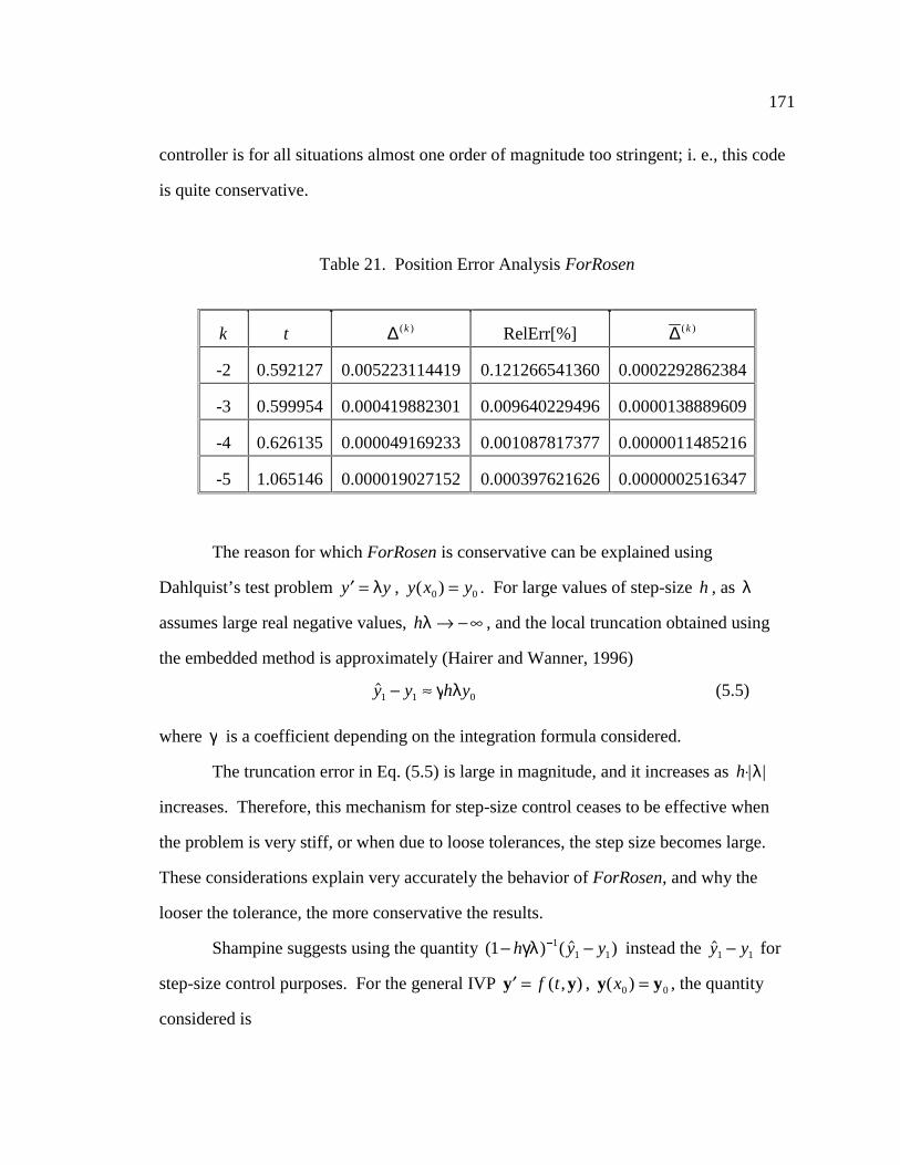
171
controller is for all situations almost one order of magnitude too stringent; i. e., this code
is quite conservative.
Table 21. Position Error Analysis ForRosen
k t ∆ ( )k RelErr[%] ∆ ( )k
-2 0.592127 0.005223114419 0.121266541360 0.0002292862384
-3 0.599954 0.000419882301 0.009640229496 0.0000138889609
-4 0.626135 0.000049169233 0.001087817377 0.0000011485216
-5 1.065146 0.000019027152 0.000397621626 0.0000002516347
The reason for which ForRosen is conservative can be explained using
Dahlquist’s test problem � =y yλ , y x y( )0 0= . For large values of step-size h , as λ
assumes large real negative values, hλ � -� , and the local truncation obtained using
the embedded method is approximately (Hairer and Wanner, 1996)
$y y h y1 1 0- £ γ λ (5.5)
where γ is a coefficient depending on the integration formula considered.
The truncation error in Eq. (5.5) is large in magnitude, and it increases as h¿| |λ
increases. Therefore, this mechanism for step-size control ceases to be effective when
the problem is very stiff, or when due to loose tolerances, the step size becomes large.
These considerations explain very accurately the behavior of ForRosen, and why the
looser the tolerance, the more conservative the results.
Shampine suggests using the quantity ( ) ( $ )1 11 1- --h y yγλ instead the $y y1 1- for
step-size control purposes. For the general IVP � =y yf t( , ) , y y( )x0 0= , the quantity
considered is

172
err I J y y= - --( ) ( $ )hγ 11 1 (5.6)
where J y= � �f is evaluated at x0 , and I is the identity matrix of appropriate
dimension. The factorization of the matrix ( )1 hγ I J- is available, since it is used to
compute stage variables k i . Therefore, err is cheap to compute. Especially for very
stiff systems, the idea of Shampine eliminates conservatism of the step-size controller.
This approach, initially in the code of Hairer and Wanner and inherited by ForSDIRK, is
currently not implemented in ForRosen.
The results in Tables 20 and 21 indicate that theoretical predictions are confirmed
by numerical results, and they underline the importance of the step-size controller. A
code with an optimistic step-size controller, may not attain the required accuracy, while
using an integrator that is too pessimistic in terms of step-size control results in excessive
computational effort.
Error analysis is also performed at the velocity level. The time variation of
angular velocity &θ1 of body 1 is shown in Figure 13.
Figure 13. Angular Velocity Body 1
-10
-7
-4
-1
2
5
8
0 2 4 6 8 10
Simulation Time [s]
An
gu
lar
Vel
oci
ty B
od
y 1
[rad
/s]

173
The angular velocity of body 1 fluctuates between –10 and 7 rad/s. The absolute
and relative tolerances were set to 10k , k = − −2 5, ,K , for all numerical experiments. The
order of magnitude for ∆ ( )k is expected to be 10 1k + .
Results in Table 22 are obtained with ForSDIRK. They confirm theoretical
predictions. The optimistic tendency of the step-size controller embedded in ForSDIRK
can be seen in these results.
Table 22. Velocity Error Analysis ForSDIRK
k t ∆ ( )k RelErr[%] ∆ ( )k
-2 0.578444 0.228908866004 3.840899692349 0.0083749741182
-3 0.291094 0.031312203070 0.427597266808 0.0009066499320
-4 0.551010 0.006406931668 0.118822262986 0.0001530648603
-5 0.136235 0.001485443259 0.017255571544 0.0000350200500
Results obtained at the velocity level with ForRosen are presented in Table 23
and they confirm the observations made earlier about this code. The step-size controller
is slightly conservative. Instead of values of 10 1- +k , the accuracy of the results as
indicated by ∆ ( )k is one order of magnitude better, most of the time.
Results presented in this Section validate the codes and confirm reliability of the
step-size controllers embedded. With one slightly on the optimistic side (ForSDIRK),
and one on the conservative side (ForRosen), the step size controllers show that the idea
of using an embedded formula for local error estimation is sound. The accuracy obtained
with these codes is good. It remains to adapt the step-size controller for ForRosen,
according to Eq. (5.6), to avoid unjustified CPU penalties.

174
Table 23. Velocity Error Analysis ForRosen
k t ∆ ( )k RelErr[%] ∆ ( )k
-2 0.795548 0.040612124932 1.844343795194 0.0016645922425
-3 0.373114 0.003792150415 0.123400255245 0.0001151519879
-4 0.217757 0.000865201346 0.009222397857 0.0000134313788
-5 0.186183 0.000234309801 0.002467113637 0.0000023859574
5.2 Explicit versus Implicit Integration
This Section contains a comparison, in terms of CPU time, of two different
numerical methods used for dynamic analysis of a High Mobility Multipurpose Wheeled
Vehicle (HMMWV). A picture of the vehicle is provided in Figure 14. The topology of
the mechanism is presented in Figure 15.
The vehicle is modeled using the same bodies as in Section 3.4.3.5, but the body
numbering of that Section is changed. Since 14 bodies are used to model this vehicle, in
what follows the model is referred as HMMWV14. More details about HMMWV
specific parameters are provided by Serban, Negrut, and Haug (1998). Finally, all timing
results in this and the following sections are obtained on a SGI Onyx machine with eight
R10000 processors.

175
Figure 14. US Army HMMWV
Figure 15. 14 Body Model of HMMWV

176
Figure 16(a) contains the original topology graph of HMMWV14. Since this
model is not stiff, stiffness is added by replacing revolute joints between upper control
arms and the chassis with spherical joints. Each joint replacement results in two
additional degrees of freedom. For each spherical joint, two Translational-Spring-
Damper-Actuators (TSDA,) acting in complementary directions model bushings that
control the extra degrees of freedom. The stiffness coefficient of each TSDA is 2 0 107. ¿
N/m, while the damping coefficient is 2 0 106. ¿ Ns/m. Tires are modeled as vertical
TSDA elements with stiffness coefficient 296325 N/m, and damping coefficient 3502
Ns/m.
Figure 16. Topology Graph for HMMWV14
The topology of the new model is presented in Figure 16(b). The stiff TSDA’s
behave like bushing elements, and induce stiffness into the model. The dominant
eigenvalue for this example has a small imaginary value, and the real part is of the order
- ¿2 6 105. .

177
The vehicle is driven straight at 10mph and hits a bump. The bump’s shape is a
half cylinder, of diameter 0.1 m. The number of degrees of freedom is 19, but the
steering rack is locked, to make sure the vehicle drives straight. This reduces the number
of degrees of freedom to 18.
The length of the simulation is from 1, to 4 seconds. Figure 17 shows the time
variation of chassis height. The front wheels hit the bump at T £ 0 5. s, and the rear
wheels hit the bump at T £ 12. s. The length of the simulation in this plot is 5 seconds.
Toward the end of the simulation (approximately after 4 seconds), due to overdamping,
the chassis height stabilizes at approximately z1 0 71= . m.
Figure 17. Chassis Height HMMWV14
The test problem is run with an explicit integrator based on the code DEABM of
Shampine and Watts, and with an implicit code based on the State-Space Reduction
Method of Section 3.2, used in conjunction with a trapezoidal formula. Among the
0.68
0.7
0.72
0.74
0.76
0 1 2 3 4 5
Time [s]
Ch
assi
s H
eig
ht
[m]

178
implicit algorithms compared in next Section, the implicit integrator used here displays
average performance.
A set of 4 tolerances is imposed, starting from a very loose value of 10-2 and
ending with a rather conservative tolerance of 10-5. Tolerances in the range 10-3 to 10-4
usually suffice in engineering applications.
Computer times required by the explicit integrator are listed in Table 24 in CPU
seconds. The code of Shampine and Watts is a multi-step code that is adapted to allow
efficient acceleration computation, based on the method proposed by Serban, Negrut,
Haug, and Potra (1997).
Table 24. HMMWV14 Explicit Integration Simulation CPU Times
TOL 10-2 10-3 10-4 10-5
1 s 3618 3641 3667 3663
2 s 7276 7348 7287 7276
3 s 10865 11122 10949 10965
4 s 14480 14771 14630 14592
Results in Table 24 confirm observations made in Section 4.2.1 concerning the
use of explicit integration formulas for stiff IVP. For the stiff test problem considered,
the performance limiting factor is stability of the explicit code. For any tolerance in the
range 10-2 through 10-5, for a given simulation length, CPU times are almost identical.
The average step-size is between 10-5 and 10-6 and it is not affected by accuracy
requirements. The code is compelled to select very small step-sizes to assure stability of
the integration process, and this is the criteria for step-size selection for a broad spectrum

179
of tolerances. Only when extremely sever accuracy constraints are imposed on
integration, is step-size limited by accuracy.
Results in Table 25 show CPU times for the implicit integrator, in seconds. A
speed-up of almost two orders of magnitude are obtained with this code.
Table 25. HMMWV14 Implicit Integration Simulation Results
TOL 10-2 10-3 10-4 10-5
1 s 42 54 122 312
2 s 79 140 330 849
3 s 92 168 400 1053
4 s 98 179 424 1095
The plot in Figure 18 shows CPU times for up to 4 seconds of simulation time.
As mentioned earlier, the vehicle clears the bump in less than 2 seconds. Since the
system is overdamped, the bounce vanishes, and the vehicle runs straight on a smooth
road. It is desired that the integrator senses that no event is taking place, and adjusts step-
size to larger values, enhancing integration efficiency. As shown in Figure 18, the
explicit code is not able to increase the step-size, and CPU time increases linearly with
simulation time. This is a limitation of the numerical method, since physically, the
evolution of the mechanical system does not pose the same transient challenges after the
bump is negotiated.
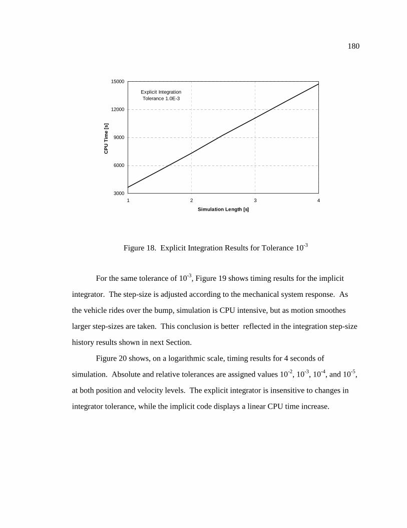
180
Figure 18. Explicit Integration Results for Tolerance 10-3
For the same tolerance of 10-3, Figure 19 shows timing results for the implicit
integrator. The step-size is adjusted according to the mechanical system response. As
the vehicle rides over the bump, simulation is CPU intensive, but as motion smoothes
larger step-sizes are taken. This conclusion is better reflected in the integration step-size
history results shown in next Section.
Figure 20 shows, on a logarithmic scale, timing results for 4 seconds of
simulation. Absolute and relative tolerances are assigned values 10-2, 10-3, 10-4, and 10-5,
at both position and velocity levels. The explicit integrator is insensitive to changes in
integrator tolerance, while the implicit code displays a linear CPU time increase.
3000
6000
9000
12000
15000
1 2 3 4
Simulation Length [s]
CP
U T
ime
[s]
Explicit IntegrationTolerance 1.0E-3

181
Figure 19. Implicit Integration Results for Tolerance 10-3
Figure 20. Timing Results for Different Tolerances
10
100
1000
10000
100000
2 3 4 5
Accuracy
Sim
ula
tio
n C
PU
Tim
e [s
]
Implicit Integrator
Explicit Integrator
0
50
100
150
200
1 2 3 4
Simulation Length [s]
CP
U T
ime
[s]
Implicit IntegrationTolerance 1.0E-3

182
5.3 Method Comparison
This Section contains a comparison of algorithms developed for implicit
integration of DAE of Multibody Dynamics. The algorithms compared are presented in
Chapter 4, and they are as follows:
(1). SspTrap, the algorithm of Section 4.1, compared in the previous Section with the
explicit code. It is based on the trapezoidal formula used in conjunction with the
State-Space Reduction Method
(2). InflSDIRK, the algorithm of Section 4.2, based on the SDIRK4/16 formula used in
conjunction with the Descriptor Form Method
(3). InflTrap, the algorithm of Section 4.3, based on the trapezoidal formula and the
Descriptor Form Method
(4). ForSDIRK, the algorithm of Section 4.5, validated in Section 5.1, and based on the
SDIRK4/15 formula used in conjunction with the First Order Reduction Method
(5). ForRosen, the algorithm of Section 4.4, validated in Section 5.1, and based on the
Rosenbrock-Nystrom formula used in conjunction with the First Order Reduction
Method
CPU results reported in seconds are obtained on an SGI Onyx machine with
R10000 processors. The simulation is identical to that in the previous Section; i. e., the
HMMWV14 model is driven at 10mph over a bump of cylindrical shape. Four tolerances
are imposed, and simulations are from 1 to 4 seconds long. The same tolerance is
imposed at both position and velocity levels.
The following four tables present timing results for InflTrap, InflSDIRK,
ForSDIRK, and ForRosen. For SspTrap, timing results are provided in Table 25.

183
Table 26. Timing Results for InflSDIRK
TOL 10-2 10-3 10-4 10-5
1 s 33 52 90 170
2 s 69 124 218 433
3 s 81 150 248 493
4 s 84 155 256 500
Table 27. Timing Results for InflTrap
TOL 10-2 10-3 10-4 10-5
1 s 42 61 158 463
2 s 79 155 420 1198
3 s 92 189 524 1521
4 s 100 206 552 1568
Table 28. Timing Results for ForSDIRK
TOL 10-2 10-3 10-4 10-5
1 s 10.1 21 33 57
2 s 25.3 49 78 139
3 s 29.5 58 92 166
4 s 30 61 94 184

184
Table 29. Timing Results for ForRosen
TOL 10-2 10-3 10-4 10-5
1 s 5.6 13.2 40.7 172
2 s 12.6 32.6 95 405
3 s 13 36.3 105 422
4 s 13.3 37 106 428
Based on the results presented in these tables, in terms of methods used for
numerical solution of DAE of Multibody Dynamics, the First Order Reduction Method is
the most efficient, while the Descriptor Form Method is the slowest. The conclusion is
that linear algebra is a key factor in deciding performance of a method. The First Order
and State-Space Reduction Methods result in algebraic problems of lower dimension,
compared to the Descriptor Form Method. In the latter method, iterations are carried out
to simultaneously solve for Lagrange multipliers and generalized accelerations. At each
iteration, this requires solution of a linear system of dimension m n+ , where m is the
number of position constraint equations, and n is the number of generalized coordinates
used to model the mechanical system. For the HMMWV14 model, n = 98 , m = 80 , and
the dimension of the discretized non-linear system of equations is 178 178� . Although
sparse linear routines of the Harwell library are used to solve this system, the penalty is
still significant.
The fastest algorithm for mild tolerances is ForRosen, which is Rosenbrock-
Nystrom formula embedded in the First Order Reduction Method. This algorithm is
more than 250 times faster than the explicit code DEABM. The algorithm requires three
function evaluations per successful time step. Practically, this number is reduced to two,

185
since one acceleration evaluation is obtained as a by-product of integration Jacobian
computation. The algorithm ceases to be efficient for stringent accuracy requirements.
However, this is a problem that can be easily fixed by adjusting the step-size controller,
according to Eq. (5.6).
For tight tolerances, ForSDIRK becomes the most efficient algorithm. It uses the
step-size controller and convergence analysis tools inherited from a code of Hairer and
Wanner. The step-size controller has a major impact on results of the simulation.
Although ForRosen and ForSDIRK both use fourth order formulas for integration and
third order formulas for step-size control, for a 1 second long simulation of the
HMMWV14 with tolerances set to 10-5, ForRosen requires 2211 successful time steps to
carry out simulation, while ForSDIRK requires 308.
Figure 21 contains a comparison of the five algorithms. For one second of
simulation, tolerance is successively set to 10-2, 10-3, 10-4, and 10-5. The same relative
and absolute tolerances are used for positions and velocities. The results are plotted on a
logarithmic scale.
For tolerances almost up to 10-4, ForRosen is the best algorithm. For higher
tolerances, ForSDIRK is the most efficient algorithm. The slopes of the two SDIRK
based algorithms are the same, and smaller than the slope displayed by the trapezoidal
based algorithms. This is explained by the lower order of the trapezoidal formula. The
conclusion is that an algorithm based on a lower order formula is not recommended for
high accuracy. The higher slopes for lower order formulas indicate a more rapid increase
in computational effort as the tolerance becomes tighter.
Results in Figure 21 underline the importance of a good integration formula,
embedded in the framework of a DAE method. The Descriptor Form Method is
characterized by more intense linear algebra, when compared with the State-Space
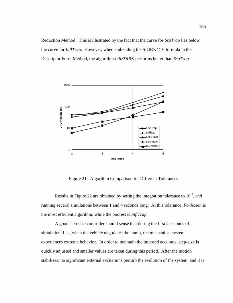
186
Reduction Method. This is illustrated by the fact that the curve for SspTrap lies below
the curve for InflTrap. However, when embedding the SDIRK4/16 formula in the
Descriptor Form Method, the algorithm InflSDIRK performs better than SspTrap.
Figure 21. Algorithm Comparison for Different Tolerances
Results in Figure 22 are obtained by setting the integration tolerance to 10-3, and
running several simulations between 1 and 4 seconds long. At this tolerance, ForRosen is
the most efficient algorithm, while the poorest is InflTrap.
A good step-size controller should sense that during the first 2 seconds of
simulation; i. e., when the vehicle negotiates the bump, the mechanical system
experiences extreme behavior. In order to maintain the imposed accuracy, step-size is
quickly adjusted and smaller values are taken during this period. After the motion
stabilizes, no significant external excitations perturb the evolution of the system, and it is
1
10
100
1000
2 3 4 5
Tolerance
CP
U R
esu
lts
[s]
SspTrap
InflTrap
InflSDIRK
ForRosen
ForSDIRK

187
expected that the step-size is increased to take advantage of the relatively smooth
evolution of the system. This is exactly what the results in Figure 22 suggest. The
curves are rather steep for short simulations, but become almost horizontal for longer
simulations. This indicates that after simulation passes the 2 second barrier, an increase
in simulation length does not significantly increase the total CPU time. The same
conclusion is supported by results in Figure 23, where for ForSDIRK and SspTrap,
simulation step-size is plotted for a 4 second long simulation. The tolerances (absolute
and relative) are set to 10-3.
Figure 22. Algorithm Comparison for Different Simulation Lengths
The algorithm ForSDIRK is based on a higher order integration formula.
Therefore, when compared to SspTrap, it is capable of taking larger step-size. The
consequence is that the first algorithm takes fewer time steps, therefore fewer integration
Jacobian computations and factorizations. One integration Jacobian evaluation accounts
10
100
1000
1 2 3 4
Simulation Length [s]
CP
U R
esu
lts
[s]
SspTrap
InflTrap
InflSDIRK
ForRosen
ForSDIRK

188
for 55% of the CPU time of a successful time step, so keeping the number of integration
Jacobian evaluations low is important. For implicit integration of the DAE of Multibody
Dynamics via the state-space formulation, one lesson that must be learned is that it is
recommended to consider more sophisticated integration formulas. This will pay off in
fewer calls to expensive integration Jacobian evaluations and factorizations, as well as
function evaluations (acceleration computations).
Figure 23. Step-Size History for ForSDIRK and SspTrap
The results in Figure 23 demonstrate that the step-size is rapidly cut to small
values when the vehicle experiences extreme motion. This is the case when the wheels
hit the bump ( T £ 0 55. s, T £ 12. s). After that, the step-size increases, and the impact of
larger step-sizes reflects in the plot of Figure 22.
0
0.01
0.02
0.03
0.04
0.05
0.06
0.07
0 1 2 3 4
Simulation Time [s]
Ste
p-S
ize
[s]
ForSDIRK
SspTrap

189
Results presented in Figure 24 show the evolution of step-size over a longer
simulation. The tolerance (absolute and relative) is set to 10-3, and the length of the
simulation is 30 seconds. Step-sizes for InflSDIRK and ForRosen very soon reach the
limit value of 1.0 s, imposed because of safety considerations. The results in this plot
clearly demonstrate the potential of the implicit algorithms developed, compared to an
explicit formula based algorithm. In particular, for the explicit code DEABM of Section
5.1, since CPU average time for one second of simulation is slightly more than 1 hour, a
simulation such as the one in Figure 24 would require more than one day of CPU time.
For ForRosen, it takes 38 seconds to complete this run
Figure 24. Step-Size History for ForRosen and InflSDIRK
The very good performance of ForRosen is due to its good order, good stability
properties, and low number of function evaluations. The order 4 was mentioned earlier to
0
0.2
0.4
0.6
0.8
1
1.2
0 5 10 15 20 25 30
Simulation Time [s]
Ste
p-S
ize
[s]
InflSDIRK
ForRosen

190
allow for larger step-sizes, and thus fewer integration Jacobian evaluations. The good
stability properties of this algorithm enable it to deal with very stiff mechanical systems.
Finally, the number of function evaluations is 3, but it was mentioned that one
acceleration evaluation comes at no price. Therefore, there are only two requests for
acceleration computation for each successful time step.
Figure 25 displays the number of iterations necessary for SspTrap to retrieve,
during each time step, the solution of the discretized system of non-linear equations. The
length of simulation is 10 seconds with tolerances set to 10-3. Compared to ForRosen,
the number of iterations, and therefore the number of function evaluations required by
SspTrap, especially during the critical part of simulation; i. e., the first 2 seconds, is large.
One function evaluation for the State-Space Method is cheaper than one function
evaluation for ForRosen, but not cheap enough to compensate for only two function
evaluations required by the latter algorithm.
The sole reason that Rosenbrock methods are not used extensively is because it
requires an exact integration Jacobian. This quantity is not always possible to compute,
and automatic differentiation or numerical means must be considered to provide
derivatives appearing in the integration Jacobian. Most frequently, obtaining force
derivatives is the difficult part, since certain force elements are either too complex, or as
in the case of multidisciplinary applications, are provided by other sub-models, with little
or no adjacent information. The algorithm ForSDIRK possesses the numerical means to
generate the entire integration Jacobian numerically. Table 30 lists CPU timing results in
seconds required for simulations when the integration Jacobian is first computed
analytically and then numerically.
Employing numerical means for integration Jacobian computation results in 4 to 5
times larger simulation CPU times. Still, it is much more advantageous to use this

191
approach, rather than to resort to explicit integration for dynamic analysis of stiff
mechanical systems.
Figure 25. Number of Iterations for SspTrap
Table 30. ForSDIRK Analytical/Numerical Computation ofIntegration Jacobian
1 second 2 seconds 3 seconds 4 seconds
Analytic 21 49 58 61
Numeric 104 229 269 278
1
3
5
7
9
0 2 4 6 8 10
Simulation Time [s]
No
mb
er o
f It
erat
ion
s
SspTrap

192
CHAPTER 6
CONCLUSIONS AND RECOMMENDATIONS
Three new methods have been developed for implicit numerical integration of the
DAE of Multibody Dynamics. Based on these methods, five algorithms were
implemented. When used for dynamic analysis of stiff mechanical systems, these
algorithms are two orders of magnitude faster than previously available integrators.
Two efficient methods for topology based linear algebra have been introduced.
For Cartesian representation of mechanical systems, the proposed algorithms enable
computation of accelerations and Lagrange multipliers 3 to 4 times faster than previous
implementations. When using a joint formulation to represent mechanical systems, the
computational time for computing accelerations is halved. The algorithms for fast
acceleration computation can be used for both explicit and First Order Reduction-based
implicit integration of the DAE of Multibody Dynamics.
Several issues remain to be investigated and/or numerically implemented, as
follows:
(a). Implement methods for parallel computation of the integration Jacobian.
(b). Investigate and implement the tangent-plane parametrization-based DAE-to-ODE
reduction method.
(c). Embed topology based linear algebra routines in numerical implementations of the
First Order Reduction Method. Currently, advantage is not taken of the subroutines
developed for fast acceleration computation.
(d). Improve stopping criteria for State-Space Reduction and Descriptor Form Methods.

193
(e). Adjust the step-size controller of the algorithm ForRosen, based on the
Rosenbrock-Nystrom formula used in conjunction with the First Order Reduction
Method, to eliminate its conservative estimate.
(f). Apply methods developed for numerical solution of systems that include flexible
bodies and intermittent motion
Appendix A and B provide details regarding the method of parallel computation
of integration Jacobian, and implicit integration of DAE of Multibody Dynamics via
tangent-plane parametrization-based state-space reduction.

194
APPENDIX A
PARALLEL COMPUTATION OF INTEGRATION JACOBIAN
In order to simplify the presentation, in this Appendix it is assumed that the vector
q¶ªn of generalized coordinates has been reordered such that the first m entries
contain dependent coordinates, while the last ndof entries contain independent
coordinates. The focus is on computing quantities J vv1 = && and J vv2 = &&&
, that were shown
in Chapter 3 to be needed for implicit integration of the SSODE of Multibody Dynamics.
The matrices J1 and J2 are computed one column at a time by first computing
the quantities &&qqm+1 through &&qqn
, and then &&&
qqm+1 through &&
&
qqn. The last ndof entries of
these vectors are the columns of the matrices J1 , and J2 , respectively.
For k ndof¶{ , , }1K , let i m k= + . Taking the derivative of the equations of
motion with respect to independent coordinate qi , yields
Mq q Mq q Q q Q qq q q q q q&& && &
&
1 6 3 8q q q q q qi i i i i i+ + + = +Φ ΦT T A Aλ λ (A.1)
The derivative of the vector of generalized coordinates with respect to
independent coordinate qi is obtained by differentiating the position kinematic constraint
equation of Eq. (3.7), to obtain
Φ Φu vu 1 0q ki+ ¿ =
where, u = [ , , , ]q q qm1 2 K T , and the vector 1kndof¶ª has all its entries zero, except the
k th entry which is 1. With H u v= -Φ Φ-1 , H h h h¢ ¶ª �[ , , , ]1 2 K ndofm ndof , u hq ki
= and
qh
1qk
ki=
�!
"$# (A.2)

195
The derivative &qqi is obtained by differentiating the velocity kinematic constraint
equation of Eq. (3.8) with respect to qi , to obtain
Φ Φq q uq q u 0& &3 8 q qi i+ =
Therefore
& &u q qu q qq qi i= - -Φ Φ1 3 8
Finally,
&
&
q
u
q
q
i
i
=
�
!
"
$
####0
0
M(A.3)
Equation (A.1) is rewritten in the form
Mq Qq&&q q ii i+ =ΦT Pλ (A.4)
where
Q Q q Mq Q qq q q q qi q qi i
P A T A= - + -&
& [ && ]1 6 3 8Φ λ (A.5)
Differentiating the acceleration kinematic constraint equation of Eq. (3.9) with
respect to qi and rearranging terms yields
Φqq&&q ii= τ P (A.6)
where
τ τ τi q qi i
P = - -&
& [ && ]q q q qq q qΦ3 8 (A.7)
Appending Eq. (A.6) to (A.4), a linear system of dimension m n+ is obtained that
provides derivatives &&qqi and λ qi
,
M
0
q Qq
q
ΦΦ
T P
iP
�!
"$##�!
"$#=
�!
"$#
&&q
q
ii
iλ τ
(A.8)

196
The linear system of Eq. (A.8) is solved ndof times for k ndof¶{ , , }1K , with
i m k= + . The coefficient matrix of Eq. (A.8) is identical to the augmented matrix of
Chapter 3, for which an efficient factorization sequence was presented in Section 3.4.2.
After the factorization is available, it is used ndof times to compute the columns of the
matrix J1 as the last ndof components of solution &&qqi of Eq. (A.8).
Computation of J2 follows the same path. For k ndof¶{ , , }1K , with i m k= + ,
equations of motion and acceleration kinematic constraint equation are successively
differentiated with respect to &qi . This yields
Mq Q q
q qq q
q q
&& &
&& &
& & & &
& &
q q q
q
i i i
i
+ =
=
Φ
Φ
T Aλ
τ(A.9)
To compute &&
qqi, the velocity kinematic constraint equation is differentiated with respect
to &qi , yielding
Φ Φu vu 1 0&&q ki+ =
Therefore &&
u hqi k= ; i. e., &&
uqi is obtained as the k th column of matrix H . Finally,
&&
qh
1qk
ki=
�!
"$# (A.10)
Introducing the notation
Q Q qqi qi
V A=& &
& , τ τi qi
V =& &
&qq (A.11)
&&&
qqi is obtained by solving
M
0
q Qq
q
ΦΦ
T V
V
�!
"$##�!
"$#=
�!
"$#
&&&
&
q
q
i
i
i
iλ τ
(A.12)
The last ndof components of &&&
qqi form the k th column of J2 . The coefficient
matrix in Eq. (A.12) is identical to the one in Eq. (A.8). This matrix is factored once and

197
then used to obtain both derivatives &&vv and &&&
vv . The pseudo-code for the proposed
algorithm is outlined in Table 31.
Table 31. Pseudo-code for Parallel Computation of Integration Jacobian
1. Evaluate and Factor Augmented Matrix
2. Evaluate Basic Derivatives
3. Compute H matrix
4. For i from m+1 to n do
5. Set k i m= -
6. Compute qqi
7. Compute &qqi
8. Compute QiP and τ i
P
9. Solve System in Eq. (A.8) for &&qqi (column k of J1 )
10. Compute QiV and τ i
V
11. Solve System in Eq. (A.12) for &&&
qqi (column k of J2 )
12. End do
Based on results of Section 3.4.2, Step 1 produces information required by the
solution sequence that is employed to solve a linear system of the form
M
0
x
y
b
bq
q
ΦΦ
T�!
"$##�!
"$# =
�!
"$#
1
2
(A.13)
The first three sub-steps to be taken are as in Algorithm 3 of Section 3.4.2.4, followed by
factorization of the reduced matrix B . The last sub-step; i. e., Step 4 , of Algorithm 3,

198
retrieves the solution of the system of Eq. (A.8) or (A.12), and is carried out after the
right side of the linear systems is available (Steps 9 and 11).
Step 2 of the pseudo-code evaluates the derivatives Mqq
&&1 6 , Φq q
Tλ3 8 , Φq qq&3 8 ,
Φq qq&&3 8 , Qq
A , Qq&A , τq , and τ
&q . During Step 3, the sub-Jacobian Φu is factored, and the
matrix H u v= - -Φ Φ1 is computed.
Step 4 starts the loop that computes the columns of matrices J1 and J2 . The
derivatives qqi and &qqi
are computed based on Eqs. (A.2) and (A.3). The right sides of
the linear systems of Eqs. (A.8) and (A.12) are obtained based on Eqs. (A.5) and (A.7),
and Eq. (A.11), respectively. The solutions of these systems provide column k of J1
and J2 . Each column is obtained as the last ndof components of the vector x ¶ªn of
Eq. (A.13). The loop ends after all ndof columns of J1 and J2 have been computed.
The advantage of using this approach versus the one described in Section 3.4.1.2,
is twofold. First, for linear systems such as in Eq. (A.13), an efficient solution sequence
is available. It is the same as that used to compute Lagrange multipliers and generalized
accelerations. The algorithm for the Cartesian formulation is presented in Section 3.4.2.
The proposed approach has two levels of parallelism. Steps 1 through 3 can be
done in parallel, since these activities are not related in any way. Step 3 can be further
distributed to parallel processors to simultaneously compute the derivatives Mqq
&&1 6 ,
Φq q
Tλ3 8 , Φq qq&3 8 , Φq q
q&&3 8 , QqA , Qq&
A , τq , and τ&q . Finally, Steps 5 through 11 are carried
out ndof times. If ndof processors are available, this task can be distributed to compute
the columns of J1 and J2 in parallel.
This proposed strategy has not been numerically implemented, and therefore no
results are available to assess to what extend it is superior to the algorithm provided in
Section 3.4.1.2. The algorithm is attractive, since usually the number ndof of degrees

199
of freedom of the model is small; and, with the fast solution sequence available for
systems such in Eq. (A.13), obtaining each of the ndof columns of J1 and J2 is fast.
From an efficiency standpoint, the proposed approach closes the gap between implicit
and explicit integration, since
(a). For explicit integration, the coefficient matrix of Eq. (A.13) must be factored once,
and one solution is computed based on factorization.
(b). For implicit integration based on the proposed algorithm for computation of the
integration Jacobian, the same coefficient matrix must be factored once, and
2 � ndof solutions corresponding to 2 � ndof different right sides are computed.
For both (a) and (b) above, the costly computation is factoring the coefficient matrix (or
equivalently, in the framework of Algorithm 3, Steps 1 through 3). Generally, retrieving
the solution of an l l� linear system when the factorization is available, reduces to a
forward/backward sequence, which is an order l2 operation. On the other hand, the
factorization is an order l3 operation. Thus, on a sequential machine, (b) requires
additional 2 1� -ndof forward/backward elimination sequences. However, what is
costly, when comparing to explicit integration, is Step 2 of the pseudo-code.
The final conclusion is that if (b) is to become competitive, compared to (a), multi-
processor architecture must be considered. Then, the impact of Step 2 is reduced, and the
extra effort related to the additional 2 1� -ndof forward/backward sequences
disappears, provided enough processors are available. Under this scenario, a Rosenbrock
formula with a small number of function evaluations, such as the one presented in
Chapter 4, could be considered for applications ranging from mildly to extremely stiff
problems. This remains to be investigated.

200
APPENDIX B
TANGENT-PLANE PARAMETRIZATION-BASED IMPLICIT INTEGRATION
In this thesis, numerical solution of the DAE of Multibody Dynamics is based on
state-space reduction technique. In the framework of state-space methods, the index 3
DAE of Multibody Dynamics induce a differential equation on the constraint manifold,
which is first projected on a subspace of the n-dimensional Euclidean space. This sub-
space is parameterized by a set of independent variables, which are called
parametrization variables. The resulting state-space ODE (SSODE) is integrated using a
classical numerical integration formula. The one-to-one local chart from the manifold to
the projection subspace is then used to determine the point on the manifold corresponding
to the solution of the SSODE.
This framework was first proposed by Rheinboldt (1984), in an effort to formalize
the theory of numerical solution of DAE, using the language of differential manifolds.
More applied considerations following this path are due to Wehage and Haug (1982),
Liang and Lance (1987), Potra and Rheinboldt (1990, 1991), and Yen (1993). What
distinguishes these methods is the choice of manifold parameterization. In Chapter 2 it
was mentioned that this thesis uses the generalized coordinate state-space reduction due
to Wehage and Haug (1982), in which parameterization variables are a subset of
generalized coordinates.
State-space methods for solution of the DAE of multibody dynamics have been
subject to critique in two aspects. First, the choice of projection subspace is generally not
global. Second, as Alishenas and Olafsson (1994) have pointed out, bad choices of the

201
projection space result in SSODE that are demanding in terms of numerical treatment,
mainly at the expense of overall efficiency of the algorithm.
The approach proposed in this Section uses the manifold tangent hyper-plane as
the projection sub-space. Parametrization variables are obtained as linear combinations
of generalized coordinates. The benefits of this reduction are anticipated to be twofold.
The resulting SSODE is expected to be numerically better conditioned and allow for
significantly larger integration step-sizes. Second, dependent variable recovery can take
advantage of information generated during the process of state-space reduction.
Tangent-space parametrization requires QR decomposition of the constraint
Jacobian, an operation that is twice as costly as Gaussian elimination used in the
coordinate partitioning technique. One possibility to diminish this difference is to take
into account the structure of the constraint Jacobian, as induced by connectivity between
bodies of the model. Sparsity and structure can be preserved and efficiently exploited by
using Givens rotation (Golub and Van Loan, 1989) for QR factorization of the constraint
Jacobian. A future research objective is to analyze to what extent the better conditioning
of the resulting SSODE compensates for the somewhat more expensive state-space
reduction stage of the tangent-plane method.
As a result of QR factorization of the constraint Jacobian Φq ¶ª �m n , a unitary
matrix Q ¶ª �n n , and a matrix R ¶ª �n m are obtained such that
Φq Q RT = ¿ (B.1)
The matrix Q is partitioned in the form
Q Q Q= [ ]1 2 (B.2)
with Q1 ¶ª �n m and Q2 ¶ª �n ndof . The matrix R assumes the form
RR
0=
�!
"$#
1 (B.3)

202
where R1 ¶ª �m m is upper triangular with non-zero diagonal elements, provided the
constraint Jacobian matrix has full row rank. The following identities are used in this
section:
Q Q 01 2T =
�m ndof , Q Q I1 1T =
�m m , Q Q I22T =
�ndof ndof (B.4)
To avoid the confusion that might be caused by using the same letter to denote
both the vector of generalized forces and the matrix in the QR factorization, the
equations of motion and kinematic constraint equations at the position, velocity, and
acceleration levels are rewritten in the form
Mq Fq&& + =ΦT Aλ (B.5)
Φ( )q 0= (B.6)
Φqq 0& = (B.7)
Φqq&& = τ (B.8)
A new set of generalized coordinates z is defined as
z Q q= T (B.9)
Let u ¶ªm contain the first m components of z and v ¶ªndof contain the last ndof
components of z . Since Q is unitary,
q Qz= (B.10)
Therefore,
q Q Qu
vQ u Q v=
�!
"$# = +[ ]1 2 1 2 (B.11)
Since the matrices Q1 and Q2 are constant,
& & &q Q u Q v= +1 2 , && && &&q Q u Q v= +1 2 (B.12)

203
The next objective is to express the equations of motion and constraint equations
in Eqs. (B.5) through (B.8) in terms of the components u and v of the new variable z .
Multiplying the equations of motion on the left by QT and using Eq. (B.12) yields
Q MQz Q Q FqT T T T A&&+ =Φ λ (B.13)
Formulated in terms of the variables u and v , Eq. (B.13) assumes the form
Q MQ u Q MQ v Q Q Fq1 1 1 2 1 1T T T T T A&& &&+ + =Φ λ (B.14)
Q MQ u Q MQ v Q Q Fq2 1 2 2 2 2T T T T T A&& &&+ + =Φ λ (B.15)
Equation (B.15) can be regarded as a set of second order SSODE in v , since all
other variables in this equation; i. e., u , &u , &&u , and λ can be expressed in terms of v and
its time derivative.
To express dependent variables in terms of v and &v , note first that using the
position kinematic constraint equation of Eq. (B.6) and Eq. (B.11)
Φ Φ( ) ( , )q u v 0= = (B.16)
Since Φ Φ Φu q u qq Q R= ⋅ = =1 1, the matrix Φu is non-singular, and the implicit function
theorem (Corwin, Szczarba, 1982) guarantees that Eq. (B.16) can be locally solved in a
neighborhood of the consistent configuration q for u as a function of v .
Next, velocity kinematic constraint equation of Eq. (B.7), assumes the expression
Φq Q u Q v 0( & & )1 2+ =
and therefore
& &u Q Q vq= --
Φ 1
1
23 8 (B.17)
Finally, using the acceleration kinematic constraint equation, &&u is obtained as the
solution of the lower triangular linear system
R u1T&& = τ (B.18)

204
With u , &u , and &&u expressed as functions of v and &v , Eq. (B.14) is used to
obtain λ in terms of v and its first and second time derivatives. The Lagrange
multipliers λ is the solution of
R Q F Q MQ R Q MQ v1 1 1 1 1 1 2λ τ= - +-T A T T T &&2 7 (B.19)
The second order ODE in v is now readily available by substituting dependent
variables into Eq. (B.15). Formally, this ODE can be brought to the form
&& ( , , & )v f v v= t (B.20)
and further reduced to a first order ODE, suitable for integration using any standard ODE
code. Derivatives J vv1 ¢ && and J vv2 ¢ &&&
must be provided. The presentation here focuses
on how to provide these quantities, in the framework of tangent-plane parametrization-
based state-space reduction of the index 3 DAE of Multibody Dynamics.
Since &&&
vv is obtained most easily, the matrix J2 is computed first. For this, Eq.
(B.15) is differentiated with respect to &v to obtain
Q MQ u Q MQ J Q Q F u Fv q v u v v2 1 2 2 2 2 2T T T T T A A&& &
& & & & &
+ + = +Φ λ 2 7 (B.21)
To obtain J2 , the quantities &&
uv , &&&
uv , and λ&v must be available. Defining
H Q Qq q= --
Φ Φ1
1
23 8 3 8 (B.22)
and taking the derivative of the velocity kinematic constraint equation of Eq. (B.7) with
respect to &v yields
&&
u Hv = (B.23)
To obtain &&&
uv , the acceleration kinematic constraint equation of Eq. (B.8) is differentiated
with respect to &v . By introducing the notation
P Q H Q= +1 2 (B.24)
the derivative &&&
uv assumes the form

205
&&& &
u HJ Q Pv q q= +-
2 1
1Φ3 8 τ (B.25)
To compute the derivative λ&v , Eq. (B.14) is differentiated with respect to &v . This yields
λ& & &
&&v q q vQ Q F P Q MQ u Q MQ J= - +-
1
1
1 1 1 1 2 2T T T A T TΦ3 8 2 7 (B.26)
Substituting Eqs. (B.23), (B.25), and (B.26) into Eq. (B.21), J2 is obtained as the
solution of the multiple right side system
P MP J P F MQ Q Pq q 1 qT T A2 7 3 82 1
1= -
-
& &
Φ τ (B.27)
The matrix J2 can be computed if the coefficient matrix in Eq. (B.27) is non-singular.
This matrix can be shown to be positive definite, provided the quadratic form 1 2 & &q MqT
is always positive for any non-zero &q satisfying velocity kinematic constraint equation.
This latter statement is not a restrictive assumption, since under these circumstances, the
above quadratic form represents the kinetic energy of the mechanical system, which is
positive for non-zero &q . Let &v ¶ªndof be an arbitrary vector. Then
& & &v P MPv v H Q Q M Q H Q vT T T T T T= + +1 2 1 22 7 1 6
Using Eqs. (B.12) and (B.22)
& &u Hv=
Therefore
Q H Q v Q u Q v q1 2 1 2+ = + =1 6 & & & &
Then,
& & & &v P MPv q MqT T T= > 0
Consequently, the coefficient matrix in Eq. (B.27) is positive definite, and the
computation of J2 is possible.

206
The computation of J vv1 = && follows the same approach used for computation of
J2 . Taking the derivative of Eq. (B.15) with respect to v yields
Q MQ u Q MQ u Q MQ Q MQ J
Q Q Q F q F q
v v v
q v q v q v q v
2 1 2 1 2 2 2 2 1
2 2 2
T T T T
T T T T T A A
&& &&
&&
2 7 2 73 8 3 8
+ + +
+ + = +Φ Φλ λ(B.28)
The quantities that must be computed are uv , &uv , &&uv , and λ v . In order to
compute uv , position kinematic constraint equation of Eq. (B.6) is differentiated with
respect to v . With the definition of the matrix H in Eq. (B.22),
u Hv = (B.29)
and based on Eqs. (B.11) and (B.24),
q Q H Q Pv = + =1 2 (B.30)
The derivative &uv is obtained by differentiating the velocity kinematic constraint
equation of Eq. (B.7) with respect to v . Rearranging the terms and taking into account
the definition of matrix P ,
& &u Q q Pv q q q= -
-
Φ Φ1
13 8 3 8 (B.31)
To compute &&uv , the acceleration kinematic constraint equation of Eq. (B.8) is
differentiated with respect to v to obtain
Φ Φq q v q v q v q vq q Q u Q J q Q u&& && &&
3 8 1 6+ + = +1 2 1 1τ τ
and, after rearranging terms,
&& && &&
u HJ Q q Q Q q Pv q q q q q q q q= + - -
- -
1 1
1
1 1
1Φ Φ Φ Φ3 8 3 8 3 8 3 8τ τ (B.32)
Finally, the derivative λ v is obtained by differentiating Eq. (B.14) with respect to v , to
obtain

207
Q MQ u Q MQ u Q MQ v Q MQ J
Q Q Q F P F Q u
v v v
q v q v q q v
1 1 1 1 1 2 1 2 1
1 1 1 1
T T T T
T T T T T A A
&& && &&
&&
2 7 2 73 8 3 8
+ + +
+ + = +Φ Φλ λ
and, after rearranging the terms,
λ λv q q v v
q q v
Q Q Mq Q MQ u
Q MQ J Q F P F Q u
= - + +
+ - +
-
1
1
1 1 1
1 2 1 1 1
T T T T T
T T A A
Φ Φ3 8 3 83 8&& &&
&&
(B.33)
Substituting the expression of the derivatives in Eqs. (B.29), (B.31), (B.32), and
(B.33) into Eq. (B.28), after matrix manipulations, J1 is obtained as the matrix solution
of the linear system
P MP J P MZ q Mq F
MZ F Z q P
q q q q q q q
q q q q
T T T A
A
2 7 3 8 1 6 3 8J3 8 3 8 L
1 = - - + -
+ -
Φ Φ
Φ
&& &&
&& &
τ λ
τ(B.34)
where
Z Q Qq=-
1 1
1Φ3 8 (B.35)
In a quasi-Newton implementation used in conjunction with a one-step method,
the integration Jacobian is evaluated once at the beginning of a macro-step. It is then
used for all stages. In this configuration, matrices H , P , and Z defined in Eqs. (B.22),
(B.24), and (B.35), respectively, assume simpler expressions because of the identities
provided in Eq. (B.4). Thus,
H 0= (B.36)
P Q= 2 (B.37)
Z Q R= -
1 1T (B.38)
When compared to the coordinate partitioning alternative, the tangent-plane
parametrization-based state-space reduction results in a different SSODE, provided in

208
implicit form in Eq. (B.15). Equations (B.27) and (B.34) provide derivative information
that is shown in Section 3.4 to be sufficient for the First Order Reduction Method. Once
the second order ODE, and derivative information are available, the First Order
Reduction Method is directly applicable.
Although the theoretical framework for the tangent-plane parameterization
algorithm was outlined several years ago (Mani, Haug, and Atkinson, 1985; Potra and
Rheinboldt, 1991), there have been no systematic numerical experiments with large scale
mechanical systems to confirm better performance in terms of integration step size and
robustness. Implementing the tangent-plane parametrization reduction algorithm and
carrying out a systematic comparison with the alternative provided by the coordinate
partitioning algorithm remains one direction of future work.
209
REFERENCES
Alexander, R., “Diagonally Implicit Runge-Kutta Methods for Stiff ODE’s,” SIAM J.Numer. Anal., vol. 14, pp. 1006-1021, 1977
Alishenas, T., “Zur Numerische Behandlung, Stabilisierung durch Projection undModellierung mechanischer Systeme mit Nebenbedingungen und Invarianten,”Doctoral Thesis, The University of Stockholm, TRITA-NA-9202, 1992
Alishenas, T., Olafsson, O., “Modeling and Velocity Stabilization of ConstrainedMechanical Systems,” BIT, Vol. 34, pp. 455-483, 1994
Andrezerjewski, T., Schwerin, R., "Exploiting Sparsity in the Integration of MultibodySystems in Descriptor Form," Preprint 95-24, Universität Heidelberg, 1995
Ascher, U., Chin, H., Petzold, L. R., Reich, S., ”Stabilization of Constrained MechanicalSystems with DAEs and Invariant manifolds,” Mech.Struct.&Mach., vol. 23(2), pp.125-157, 1995
Ascher, U., Petzold, L. R., “Stability of Computational Methods for ConstrainedDynamics Systems,” SIAM J. Sci., Stat. Comput, vol. 14, pp. 95-120, 1993
Ascher, U., Petzold, L. R., Chin, H., “Stabilization of DAEs and invariant manifolds”,submitted to, Numer. Math. 1994
Atkinson, K. E., An Introduction to Numerical Analysis, New York: John Wiley & Sons,2nd Edition, 1989
Axelsson, O., “A note on a class of strongly A-stable methods,” BIT, vol. 12, pp. 1-4,1972
Bader, G., Deuflhard, P., “A semi-implicit mid-point rule for stiff systems of ordinarydifferential equations,” Numer. Math., vol. 41, pp. 373-398, 1983
Baumgarte, J., “Stabilization of constraints and integrals of motion in dynamicalsystems,” Comp. Meth. In Appl. Mech. and Eng., vol. 1, pp. 1-16, 1972
Bischof, C., Carle, A., Khademi, P., Mauer, A., “The ADIFOR2.0 System for theAutomatic Differentiation of Fortran77 Programs,” Argonne Preprint ANL-MCS-P481-1194, 1994
Brankin, R. W., Gladwell, I., Shampine, L. F., “Starting BDF and Adams Codes atOptimal Order,” J. Comp. Appl. Math., vol. 21, pp. 357-368, 1988

210
Brasey, V., “Half-explicit method for semi-explicit differential-algebraic equations ofindex 2,” Thesis No. 2664, Sect. Math., University of Geneva, 1994
Brenan, K. E., Campbell, S. L., Petzold, L. R., The Numerical Solution of Initial ValueProblems in Ordinary Differential-Algebraic Equations. New York: North HollandPublishing Co., 1989
Brown, P. N., Byrne, G. D., Hindmarsch, A. C., “VODE: a variable coefficient ODEsolver,” SIAM J. Sci., Stat. Comput., vol. 10, pp. 1038-1051, 1989
Corwin, L. J., Szczarba, R. H., Multivariable Calculus, New York: Marcel Dekker, 1982
DADS Reference Manual, Revision 8.0, CADSI, Coralville, Iowa, 1995
Dahlquist, G., “A special stability problem for linear multistep methods,” BIT, vol. 3, pp.27-43, 1963
Dormand, J. R., Prince, P. J., “A family of embedded Runge-Kutta formulae,” J. Comp.Appl. Math., vol. 6, pp. 19-26, 1980
Duff, I. S., “Harwell MA28 - A set of FORTRAN subroutines for sparse unsymmetriclinear equations,” Report AERE-R8730, 1980
Ehle, B. L., “High order A-stable methods for the numerical solution of systems of DEs,”BIT, vol. 8, pp. 276-278, 1968
Eich, E., “Convergence results for a coordinate projective method applied to mechanicalsystems with algebraic constraints,” SIAM J. Numer. Anal., vol. 30, pp. 1467-1482,1993
Eich, E., Fuhrer, C., Leihmkuhler, B. J., Reich, S., “Stabilization and Projection Methodsfor Multibody Dynamics,” Helsinki University of Technology, Institute ofMathematics, Research Report A281, 1990
Eich, E., Fuhrer, C., Yen, J., “On the Error Control for Multistep Methods Applied toODEs with Invariants and DAEs in Multibody Dynamics,” Mech. Struct.&Mach.,vol.23(2), 1995
Fuhrer, C., Leihmkuhler, B. J., “Numerical Solution of Differential-Algebraic Equationsfor Constraint Mechanical Motion,” Numerische Mathematik, vol. 59, pp. 5-69, 1991
Gear, C. W., Numerical Initial Value Problems in Ordinary Differential Equations,Prentice Hall, 1971
Gear, C. W., Gupta, G. K., Leihmkuhler, B. J., ”Automatic Integration of the Euler-Lagrange Equations with Constraints,” J. Comp. Appl. Math., vol.12&13, pp. 77-90,1985
Golub, G. H., Van Loan, C. F., Matrix Computations, John Hopkins University Press,1989

211
Hairer, E., Nørsett S. P., Wanner, G., Solving Ordinary Differential Equations I. NonstiffProblems, Berlin Heidelberg New York: Springer-Verlag, 1993
Hairer, E., Wanner, G., Solving Ordinary Differential Equations II. Stiff andDifferential-Algebraic Problems, Berlin Heidelberg New York: Springer-Verlag,1996.
Haug, E. J., Computer-Aided Kinematics and Dynamics of Mechanical Systems. Boston,London, Sydney, Toronto: Allyn and Bacon, 1989
Haug, E. J., Negrut, D., Engstler, C., “Runge-Kutta Integration of the Equations ofMultibody Dynamics in Descriptor Form,” in preparation, 1998
Haug E. J., Negrut, D., Iancu, M., “A State-Space Based Implicit Integration Algorithmfor Differential-Algebraic Equations of Multibody Dynamics,” Mech. Struct.&Mach.,vol. 25(3), pp. 311-334, 1997(a)
Haug E. J., Negrut, D., Iancu, M., “Implicit Integration of the Equations of MultibodyDynamics,” in Computational Methods in Mechanical Systems, J. Angeles and E.Zakhariev eds., NATO ASI Series: Springer-Verlag, vol. 161, pp. 242-267, 1997(b)
Haug, E. J., Yen, J., “Implicit Numerical Integration of Constrained Equations of MotionVia Generalized Coordinate Partitioning,” J. Mech. Design, vol. 114, pp. 296-304,1992
Horn, M. K., “Forth and fifth-order scaled Runge-Kutta algorithms for treating denseoutput,” SIAM J. Numer. Anal., vol. 20, pp. 558-568, 1983
Iancu, M., Haug, E. J., Negrut, D., “Implicit Numerical Integration of the Equations ofStiff Multibody Dynamics: Descriptor Form,” in Proceeding of the NATO AdvancedStudy Institute in Computational Methods in Mechanisms, vol. II, pp. 91-99, J.Angeles and E. Zakhariev eds., Varna, Bulgaria, 1997
Kaps, P., Rentrop, P., "Generalized Runge-Kutta methods of order four with step-sizecontrol for stiff ordinary differential equations,” Numer. Math., vol. 33, pp. 55-68,1979
Krogh, F. T., “A variable step variable order mutistep method for the numerical solutionof ordinary differential equations,” Information Processing, North-Holland,Amsterdam, vol. 68, pp. 194-199, 1969
Lapack Users’ Guide, SIAM, Philadelphia, 1992
Lewis, G. L., “Implementation of the Gibbs-Poole-Stockmeyer and Gibbs-Kingalgorithms,” ACM Trans. on Math. Soft., vol. 8, pp. 180-189, 1982
Liang, G. G., Lance, G. M., “A Differentiable Null Space Method for ConstrainedDynamic Analysis,” ASME Journal of Mechanisms, Transmissions, and Automationin Design, vol. 109, pp. 405-411, 1987

212
Lubich, C., “Extrapolation Methods for Constrained Multibody Systems,” TechnicalReport A-6020, University of Innsbruck, Institute for Mathematics and Geometry,Innsbruck, 1990
Lubich, C., “Extrapolation integrators for constrained multibody systems,” Impact Comp.Sci. Eng., vol. 3, pp. 213-234, 1991
Lubich, C., Nowak, U., Pohle, U., Engstler, C., “MEXX-numerical software for theintegration of constrained mechanical multibody systems,” Preprint SC 92-12,Konrad-Zuse-Zentrum, Berlin, 1992
Mani, N. K., Haug, E. J., Atkinson, K. E., “Application of Singular Value Decompositionfor the Analysis of Mechanical System Dynamics,” ASME Journal of Mechanisms,Transmissions, and Automation in Design, vol. 107, pp. 82-87, 1985
NADS Vehicle Dynamics Software, vol. 2, Release 4, Center for Computer AidedDesign, The University of Iowa, 1995
Negrut, D., Haug, E. J., Iancu, M., “Variable Step Implicit Numerical Integration of StiffMultibody Systems,” in Proceeding of the NATO Advanced Study Institute inComputational Methods in Mechanisms, vol. II, pp. 157-166, J. Angeles and E.Zakhariev eds., Varna, Bulgaria, 1997
Negrut, D., Serban, R., Potra, F. A., “ A Topology Based Approach for ExploitingSparsity in Multibody Dynamics,” The University of Iowa, Dept. of Mathematics,Report No. 84, Dec. 1995
Negrut, D., Serban, R., Potra, F. A., “A Topology Based Approach for ExploitingSparsity in Multibody Dynamics: Joint Formulation,”, Mech. Struct.&Mach, vol.25(2), pp. 221-241, 1997
Nordsieck, A., “On numerical integration of ordinary differential equations,” Math.Comp., vol. 16, pp. 22-49, 1962
Nørsett, S. P., Wolfbrandt, A., “Order Conditions for Rosenbrock Types Methods,”Numer. Math., vol. 38, pp. 193-208, 1979
Ostermeyer, G. P., “Baumgarte stabilization for differential algebraic equations”. InNATO Advance Research Workshop in Real-Time Integration Methods forMechanical System Simulation, E. Haug and R. Deyo, eds. Berlin Heidelberg NewYork: Springer-Verlag, 1990
Petzold, L. R., “Differential/Algebraic Equations are not ODE’s”, SIAM J. Sci., Stat.Comput., vol. 3(3), pp. 367-384, 1982
Potra, F. A., “Implementation of linear multistep methods for solving constrainedequations of motion,” SIAM. Numer. Anal., vol. 30(3), pp. 474-489, 1993
Potra, F. A., “Numerical Methods for the Differential-Algebraic Equations withApplication to Real-Time Simulation of Mechanical Systems,” ZAMM, vol. 74(3), pp.177-187, 1994

213
Potra, F. A., Rheinboldt, W. C., “Differential-Geometric Techniques for SolvingDifferential Algebraic Equations,” In Real-Time Integration of Mechanical SystemSimulation, E. Haug and R. Deyo, eds., Springer-Verlag, Berlin, 1990
Potra, F. A., Rheinboldt, W. C., “On the numerical solution of Euler-Lagrangeequations,” Mech. Struct. & Mech., vol. 19(1), pp. 1-18, 1991
Prothero, A., Robinson, A., “On the stability and accuracy of one-step methods forsolving stiff systems of ordinary differential equations,” Math. of Comput., vol. 28,pp. 145-162, 1974
Rheinboldt, W. C., “Differential-Algebraic Systems as Differential Equations onManifolds,” Math. Comp., vol. 43, pp. 473-482, 1984
Sandu, A., Negrut, D., Haug, E. J., Potra, A., Sandu, C., “A Rosenbrock Method for StateSpace Based Integration of Differential Algebraic Equations of MultibodyDynamics,” in preparation, 1998
Schiehlen, W., Multibody Systems Handbook. Berlin, Heidelberg, New York: Springer-Verlag, 1990
Serban, R., “Dynamic and Sensitivity Analysis of Multibody Systems,” Ph.D. Thesis,The University of Iowa, 1998
Serban, R., Negrut, D., Haug, E. J., “HMMWV Multibody Models,” Technical Report R-211, Center for Computer-Aided Design, The University of Iowa, 1998
Serban, R., Negrut, D., Haug, E. J., Potra, F. A., "A Topology Based Approach forExploiting Sparsity in Multibody Dynamics in Cartesian Formulation,” Mech.Struct.&Mach., vol. 25(3), pp. 379-396, 1997
Shampine, L. F., “Implementation of implicit formulas for the solution of ODEs,” SIAMJ. Sci. Stat. Comput., vol. 1, pp. 103-118, 1980
Shampine, L. F., “Conservation Laws and the Numerical Solution of ODEs,” Comp. AndMath. With Appls., vol. 12B, pp. 1287-1296, 1986
Shampine, L. ,F., Numerical Solution of Ordinary Differential Equations, Chapmann &Hall, New York, 1994
Shampine, L. F., Gordon, M. K., Computer Solution of Ordinary Differential Equations.The Initial Value Problem, Freeman and Company, San Francisco, 1975
Shampine, L. F., Watts, H. A., “The art of writing a Runge-Kutta code.II,” Appl. Math.Comput., vol. 5, pp. 93-121, 1979
Shampine, L. F., Zhang, W., “Rate of Convergence of Multi-step Codes Started byVariation of Order and Step-size,” SIAM J. Numer. Anal., vol. 27, pp. 1506-1518,1990

214
Tsai, F. F., “Automated methods for high-speed simulation of multibody dynamicsystems,” Ph.D. Thesis, The University of Iowa, 1989
Verner, J. H., “Explicit Runge-Kutta methods with estimates of the local truncationerror,” SIAM J. Numer. Anal., vol. 15, pp.772-790, 1978
Wehage, R. A., Haug, E. J., “Generalized Coordinate Partitioning for DimensionReduction in Analysis of Constrained Dynamic Systems,” J. Mech. Design, vol. 104,pp. 247-255, 1982
Winckler, M. J., “Semiautomatic Discontinuity Treatment in FORTRAN77-Coded ODEModels,” in Proceedings of the 15th IMACS World Congress 1997 on ScientificComputation Modeling and Applied Mathematics, 1997
Yen, J., “Constrained Equations of Motion in Multibody Dynamics as ODEs onManifolds,” SIAM J. Numer. Anal., vol. 30, pp. 553-568, 1993