Computing Validated Solutions of Implicit Differential Equations

Advances in Computational Mathematics 19: 231–253, 2003. 2003 Kluwer Academic Publishers. Printed in the Netherlands.

Computing validated solutions of implicit differentialequations ∗

Jens Hoefkens a, Martin Berz a and Kyoko Makino b

a Department of Physics and Astronomy, and National Superconducting Cyclotron Laboratory,Michigan State University, East Lansing, MI 48824-1321, USA

E-mail: {hoefkens;berz}@msu.edub Department of Physics, University of Illinois at Urbana-Champaign, Urbana, IL 61801-3080, USA

E-mail: [email protected]

Received 16 November 2001; accepted 10 October 2002Communicated by C.A. Micchelli

Ordinary differential equations (ODEs), including high-order implicit equations, describeimportant problems in mechanical and chemical engineering. However, the use of self-validated methods providing rigorous enclosures of the solution has mostly been limited toexplicit and weakly nonlinear problems, and no general-purpose algorithm for the validatedintegration of general ODE initial value problems has been developed. Since most integrationtechniques for Differential Algebraic Equations (DAEs) are based on transformation to im-plicit ODEs, the integration of DAE initial value problems has traditionally been restricted tofew hand-picked problems from the relatively small class of low-index systems. The recentlydeveloped Taylor model method combines high-order differential algebraic descriptions offunctional dependencies with intervals for verification. It has proven its power in several ap-plications, including verified integration of ODEs under avoidance of the wrapping effect.Recognizing antiderivation (integration) as a natural operation on Taylor models yields meth-ods that treat DEs within a fully differential algebraic context as implicit equations made ofconventional functions and antiderivation. This method has the potential to be applied to high-index DAE problems and allows the computation of guaranteed enclosures of final conditionsfrom large initial regions for large classes of initial value problems. In the framework of thismethod, a Taylor model represents the highest derivative of the solution function occurring inthe DE and all lower derivatives are treated as antiderivatives of this Taylor model. Conse-quently, one obtains a set of implicit equations involving only the highest derivative. Utilizingmethods of verified inversion of functional dependencies described by Taylor models allowsthe computation of a guaranteed enclosure of the solution in the form of a Taylor model. Theperformance of the method is illustrated by detailed examples.

Keywords: differential algebraic equations, Taylor model, self-validated methods, intervalmethods

∗ Supported in part by the U.S. Department of Energy under contract DE-FG02-95ER40931 and the AlfredP. Sloan Foundation.

232 J. Hoefkens et al. / Solutions of implicit differential equations

1. Introduction

Under certain conditions, the solutions of ordinary differential equations (ODEs)and differential algebraic equations (DAEs) can be expanded in Taylor series in boththe independent variable and the initial conditions. In these cases, we can obtain goodapproximations of the solutions by computing the respective Taylor polynomials [14,15].Utilizing the Taylor model approach as summarized in this paper often allows us tocompute rigorous enclosures of the solutions of initial value problems [10,30].

By using index analysis [40,41] and computational differentiation, a given DAEcan often be transformed into an equivalent system of implicit ODEs. If the derivedsystem is described by a Taylor model, representing each derivative by an independentvariable, verified inversion methods [7,22] can be utilized to solve for the highest deriv-atives as functions of lower order ones. The resulting Taylor model forms an enclosureof the right-hand side of an explicit ODE initial value problem that is equivalent tothe original problem. While this explicit system is suitable for integration with Taylormodel solvers [10], the intermediate inversion often requires a substantial increase in thedimensionality of the problem, limiting the approach to relatively small systems. An ap-plication of this inversion-based integration of differential equations has been discussedin [23].

In this paper we derive a method for the verified integration of general implicitODEs that is based on the observation that solutions can be obtained as fixed points of acertain operator containing antiderivation. We show that this operator is particularly wellsuited for practical applications in Taylor model settings, since its restriction to Taylorpolynomials is guaranteed to converge to the exact nth order expansion of the solutionin at most n + 1 steps, where n ∈ N is the order of the Taylor models.

While sophisticated methods have been developed for the numerical integration ofDAE problems [1,13,18,19], they are usually based on multistep methods and generallydo not provide the possibility of verification and validation. However, since our proposedmethod of integrating implicit ODE initial value problems can also be used for the com-putation of the differentiation index νd of DAEs [1], it can be utilized for a verified indexanalysis. Combining this with methods of computational differentiation, we can obtaina scheme for transforming DAEs into implicit ODEs, which can be solved with the newmethod. Since this combination uses verified Taylor models at every stage of the com-putation, it can be used to compute Taylor model enclosures of the solutions of DAEs.By utilizing high order Taylor models (n > 20 is not uncommon), the scheme can evenbe applied to high-index problems that pose serious challenges to existing non-verifiedDAE integration methods.

2. Computational tools

In this section we summarize the theory behind the computational methods thatform the basis of the new integration scheme. First we introduce an algebra with threeoperations, including the derivative operation (derivation). Such structures are generally

J. Hoefkens et al. / Solutions of implicit differential equations 233

called differential algebras [26,42,43] and we will focus mostly on nDv which enablesus to efficiently manipulate Taylor polynomials with floating point coefficients. Then,in section 2.2, we briefly discuss interval methods and summarize the Taylor model ap-proach that combines high-order floating point polynomials with intervals. Taylor mod-els provide self-validated computations with high-order convergence and can often out-perform conventional intervals in terms of sharpness and computational cost.

2.1. The differential algebra nDv

Let U ⊂ Rv be an open set containing the origin and consider the space

Cn+1(U,Rw) of (n+1)-times continuously differentiable functions that map U into R

w.We define the relation of equality up to order n as follows.

Definition 1. For f, g ∈ Cn+1(U,Rw) we say that f equals g up to order n if f (0) =

g(0), and all partial derivatives of orders up to n agree at the origin. If f equals g up toorder n, we denote that by f =n g.

It is easy to see that equality up to order n establishes an equivalence relation onthe space Cn+1(U,R

w) [4]. The resulting equivalence classes are called DA vectors, andthe class containing the function f ∈ Cn+1(U,R

w) is denoted by [f ]n. The collection ofthese equivalence classes is called nDv. More details on this structure are given in [2,4].

Proposition 1. For f ∈ Cn+1(U,Rw), the nth order Taylor polynomial Tn(f ) of f is

contained in [f ]n.

This assertion follows easily from the basic definition of the equivalence classes.However, the fact that the nth order Taylor polynomial of f can be used as a represen-tative for the class [f ]n opens the door for a computer implementation of the structurenDv by storing and manipulating the coefficients of Taylor polynomials.

2.1.1. Elementary operations and functionsElementary operations like “+” and “×” can be lifted from Cn+1(U,R

w) in theusual way, and extend to the corresponding operations “⊕” and “⊗” on nDv [2,3].

Definition 2. Let f, g ∈ Cn+1(U,Rw) be two functions. Then the sum of the DA vectors

[f ]n and [g]n is given by

[f ]n ⊕ [g]n = [f + g]n. (1)

The product of the two DA vectors is defined by

[f ]n ⊗ [g]n = [f × g]n. (2)

Together with the scalar multiplication r · [f ]n = [r · f ]n, this definition of theelementary operations makes nDv an algebra [4] and provides a transparent extension to


the equivalence classes of DA vectors; i.e., knowledge of the values and derivatives of fand g at the origin is sufficient to obtain Taylor polynomials of their sums and products.Moreover, in [2,3] the available operations on nDv have been extended to include sub-traction and, for a limited class of DA vectors, even the multiplicative inversion. Fromnow on we omit the distinction between the operations on Cn+1(U,R

w) and nDv and willalways use the same symbols “+” and “×” for operations between numbers, functions,and DA vectors.

To fully utilize the differential algebra nDv, especially in numerical analysis andcomputer environments, it is necessary to extend the standard mathematical functionscommonly available on computers to nDv: square root, exponential, logarithm, trigono-metric and hyperbolic functions. Details on the exact definition and implementations ofthese functions have been presented in [4] and for the purposes of this paper it sufficesto say that all computer functions have in fact been extended to nDv.

It has been shown that the derivative operation can be extended from Cn+1(U, Rw)

to the algebra nDv in such a way that nDv becomes a differential algebra [2,4]. Whilewe will not use this intrinsic structure of nDv, we will make frequent use of the anti-derivation of DA vectors to be presented in section 2.1.3.

2.1.2. Contracting operators and fixed pointsIn the previous section we have shown how elementary operations on the function

space Cn+1(U,Rw) are extended to the differential algebra nDv. Here we take a look at

the more general concept of operators on nDv and summarize an important fixed pointtheorem. The availability of this powerful fixed point theorem for operators on nDv

allows the use of the differential algebra nDv in a large class of numerical applications,ranging from the analysis of dynamical systems [5,9,12] to global optimization [25,34].

Definition 3. For [f ]n ∈ nDv, the depth λ([f ]n) is defined to be the order of the firstnon-vanishing derivative of f if [f ]n �= 0, and n + 1 otherwise.

By definition of the equivalence classes, this definition is independent of the choiceof f ∈ [f ]n. We note that any a ∈ nDv with λ(a) � 1 satisfies the condition an+1 = 0and is therefore called nilpotent. Using the straightforward definition of the depth, con-tracting operators on nDv are defined as follows.

Definition 4. Let O be an operator defined on M ⊂ nDv. O is contracting on M, if forany two [f ]n, [g]n ∈ M,

λ(O

([f ]n) − O

([g]n))

� λ([f ]n − [g]n

)(3)

with equality if and only if f =n g.

This definition has a striking similarity to the corresponding definitions on stan-dard function spaces. Even more so, a theorem that resembles the Banach Fixed PointTheorem can be established on nDv. However, unlike in the case of the Banach Fixed


Point Theorem, in nDv the sequence of iterates is guaranteed to converge in at most n+1steps [4].

Theorem 1 (DA Fixed Point Theorem). Let O be a contracting operator defined onM ⊂ nDv that maps M into itself (i. e., O(M) ⊂ M). Then O has a unique fixed pointa ∈ M. Moreover, for any a0 ∈ M it is O(n+1)(a0) = a.

A proof and further discussion of the DA Fixed Point Theorem can be found in [4].Here we just mention that, since λ(a + b) � min(λ(a), λ(b)), it follows easily that thesum and composition of two contracting operators O1 and O2 defined on M is also acontracting operator.

2.1.3. AntiderivationWe conclude this section on functions on nDv with an example of an operator that

is unusual but, considering the structure of the differential algebra nDv, actually quitenatural. The antiderivation; i.e., the integration with respect to any of the v variables,turns out to be a contracting operation on nDv.

Proposition 2 (Antiderivation is contracting). For k ∈ {1, . . . , v}, the antiderivation∂−1k : nDv → nDv is a contracting operator on nDv.

The proof of this important result is based on the fact that if a, b ∈ nDv agree up toorder l, the first non-vanishing derivative of ∂−1

k (a − b) is of order l + 1 [4,23,24]. It isimportant to realize that in the DA framework of nDv, antiderivation is easily computedand there is no fundamental difference between any of the standard mathematical func-tions and antiderivation. In fact, fully embracing antiderivation as a normal operationon DA vectors will enable us to develop a new and powerful method for the verified in-tegration of ordinary differential equations (ODEs) and differential algebraic equations(DAEs) in the remainder of this paper.

2.2. Rigorous numerical analysis with Taylor models

The relative accuracy of floating point number representations on computers islimited, usually to around 16 decimal digits. Interval analysis takes this limitation intoaccount and allows the computation of guaranteed enclosures for computational results:the result of every interval computation consists of two numbers; one is guaranteed to besmaller than the mathematically correct result, the other one is guaranteed to be largerthan the correct result. Thus, if xr is the analytical result of some computation C, andR = [xl, xu] is the corresponding result of interval analysis, then xr ∈ R. On the otherhand, interval analysis can also be seen as a computerization of set theory: starting withI = [xl, xu] and some computation C, the result C(I ) = [yl, yu] contains the result ofthe computation C applied to every number contained in I . Further details on intervalanalysis can be found in [20,36,37].


Recently, Taylor models have been developed [30,31] as a combination of the highorder Taylor polynomials described in the previous subsection and interval analysis toobtain guaranteed enclosures of functional descriptions. Details on applications of thesemethods in beam physics are given in [29,35]. It has been shown [32] that the Tay-lor model approach can often substantially alleviate the following problems inherent inconventional interval arithmetic:

• sharpness for large domain intervals,

• cancellation and dependency problem,

• dimensionality curse.

2.2.1. Taylor model methodsCommonly, we view Taylor models as sets of functions that are close to a reference

polynomial as outlined below.

Definition 5. Let D ⊂ Rv be a box with x0 ∈ D. Let P : D → R

w be a polynomial oforder n and R ⊂ R

w be an non-empty convex compact set. Then (P, x0,D, R) is calleda Taylor model of order n with expansion point x0 over D.

Following these notations, P is called the reference polynomial and R is called theremainder bound of the Taylor model. We say that f is contained in a Taylor modelT = (P, x0,D, R) if P(x) − f (x) ∈ R for all x ∈ D and the nth order Taylor series off around x0 equals P .

Methods have been developed to extend mathematical operations and functionsto Taylor models such that the inclusion relationships are preserved. For example, fortwo given Taylor models, T1 and T2, the following theorem lays the foundation for thecomputation of Taylor models for the sum S, and the product P , of T1 and T2. In thecontext of this theorem B(P,D) denotes a bound for the polynomial P over the compactset D, P(n) stands for the truncation of P to order n, and P(n+) consists of the terms ofdegree larger than n in P .

Theorem 2. Let T1 = (P1, x0,D, R1) and T2 = (P2, x0,D, R2) be two Taylor modelsof order n and define

RP = R1 · R2 + R1 · B(P2,D) + B(P1,D) · R2 + B((P1 · P2)(n+),D

). (4)

Obtain new Taylor models TS and TP by

TS = (P1 + P2, x0,D, R1 + R2), (5)

TP = ((P1 · P2)(n), x0,D, RP

). (6)

Then, TS and TP are Taylor models for the sum TS and product TP of T1 and T2. Inparticular, for two functions f1 ∈ T1 and f2 ∈ T2, it is

(f1 + f2) ∈ TS and (f1 · f2) ∈ TP. (7)


Proof. If we define Cn+1 functions δ1 = f1 − P1 and δ2 = f2 − P2, then δ1(x) ∈ R1

and δ2(x) ∈ R2 for any x ∈ D. Thus, for a given x ∈ D((f1 + f2) − (P1 + P2)

)(x) = δ1(x) + δ2(x) ∈ R1 + R2 = RS. (8)

Since the nth order Taylor expansion of the sum f1 + f2 equals the sum of the Taylorseries, TS is indeed a Taylor model for the sum T1 + T2. Also, over the domain D(

(f1 · f2) − (P1 · P2)(n)) = (

(P1 + δ1)(P2 + δ2)) − (

(P1 · P2) − (P1 · P2)(n+)

)=P1 · δ2 + δ1 · P2 + δ1 · δ2 + (P1 · P2)(n+). (9)

Moreover, since the nth order Taylor polynomial of f1 ·f2 equals the polynomial product(P1 · P2)(n), TP is a Taylor model for the product T1 · T2. �

Similarly, other elementary operations and intrinsic functions can been extendedto Taylor models such that the fundamental inclusion properties of Taylor models aremaintained. For example, the exponential function of Taylor models has been defined insuch a way that for a given Taylor model T and its Taylor model exponential TE

f ∈ T ⇒ exp(f ) ∈ TE (10)

Further information on arithmetic and intrinsic functions on Taylor models can be foundin [8,31,32].

Lastly, antiderivation, which is essentially the integration operation, extends natu-rally to Taylor models. It allows us to compute a Taylor model TI from a given Taylormodel T such that TI contains primitives for each function f contained in T . Since theantiderivation does not fundamentally differ from other intrinsic functions on the set ofTaylor models, it is often used in fundamental Taylor model algorithms. An importantapplication of the antiderivation will be presented in section 2.2.2.

A consequence of the results summarized in this subsection is that we can com-pute Taylor models for any sufficiently smooth algorithm or computer function. Thisresult follows directly by finite induction from theorem 2 and similar results for intrinsicfunctions and the antiderivation:

Theorem 3. Let f : D ⊂ Rv → R

w be a sufficiently smooth function that is computableby a finite number of elementary operations, intrinsic functions, and antiderivations.Then, starting with Taylor models for the identity functions x = (x1, . . . , xv) ∈ D �→ xk ,a guaranteed enclosure of f can be obtained as a Taylor model by evaluating the codelist of f with Taylor model operations.

We close this introduction to Taylor model methods by noting that a major ad-vantage of Taylor model methods over regular interval analysis is that the sharpness ofthe enclosures obtained by Taylor models scales with the (n + 1)st order of the domainsize [7]. Thus, the Taylor model approach is of particular advantage in the combinationof Taylor models with high-order map codes like COSY Infinity [9,11] and gives smallguaranteed enclosures even for complicated high-order maps in many variables.


2.2.2. Verified enclosures of flowsOne of the most important applications of Taylor models stems from their applica-

bility to numerical ODE integration. To illustrate the method, we consider the initialvalue problem

x′ = f (t, x) and x(t0) = x0. (11)

It is a well-known fact that the solution to (11) can be obtained as the fixed point of thePicard operator O, defined by

O(x) = x0 +∫ t

t0

f (τ, x) dτ. (12)

Using the previously mentioned antiderivation, the operator O can be extended to Taylormodels and yields an algorithm that allows the computation of verified enclosures offlows M(t, t0, x0) of (11). This approach has been presented in [10,30] and has recentlybeen used successfully in a variety of applications ranging from solar system dynamics[12,21] to beam physics. Unlike methods that use conventional interval computationsto enclose the final conditions, the Taylor model approach avoids the wrapping effectto very high order and is therefore capable of propagating extended initial regions overlarge integration intervals.

3. Validated integration of general differential equations

While sophisticated general-purpose methods for the verified integration of explicitfirst order ODEs have been developed [10,27,28,30,38,39], none of these can be readilyused for the verified integration of implicit ODEs, let alone differential algebraic equa-tions. As a first step toward the verified integration of general DAEs, we consider theproblem of integrating the implicit ODE initial value problem F(t, x, x′) = 0. Unlike instandard ODE integration methods, we will not limit ourselves to first order problems,but will eventually be able to integrate the arbitrary order problem

F(t, x, x′, . . . , x(p)

), (13)

where the derivative of F with respect to the highest derivatives in each of the compo-nents is assumed to be nonsingular for all argument values in an appropriate domain.

Our integration method is based on an extended use of antiderivation. To motivatethe combination of high order methods and antiderivation for the verified integrationof general differential equations, consider the explicit second order ODE initial valueproblem

x′′ = f (x, x′, t), x(t0) = x0, x′(t0) = x′0. (14)


While the conventional approach to solving this system is based on order reduction to atwo-dimensional first order problem, in the framework of Taylor models we can use theintrinsic antiderivation and substitute ξ = x′; i.e.,

x(t) = x0 +∫ t

t0

ξ(τ) dτ. (15)

After inserting the expanded expression for x(t) into (14), we obtain an explicit expres-sion for ξ ′ in the form of a relatively simple integro-differential equation.

ξ ′ = F(ξ, t) = f

(x0 +

∫ t

t0

ξ(τ) dτ, ξ, t

). (16)

This system can readily be integrated with the existing Taylor model based integrationscheme discussed in [10,30], and the solution x(t) of (14) can be computed from theTaylor model for ξ(t) by a final application of antiderivation.

x = x0 +∫ t

t0

ξ(τ) dτ. (17)

While this approach seems obvious from a theoretical point of view, numericalanalysis has traditionally avoided explicit references to antiderivation in its algorithms.And while symbolic tools make sophisticated use of antiderivation, they often sufferfrom large memory requirements and slow computations. However, differential alge-braic frameworks [26,43] make the explicit use of antiderivation in numerical computa-tions feasible by allowing fast computations with moderate memory requirements. Froma practical point of view, the approach of using antiderivation has the advantage of reduc-ing the computational complexity of the right-hand side of the ODE (14), often allowingfor favorable computations.

3.1. High order Taylor model solutions

In this section we present a Taylor model-based algorithm for the self-validatedintegration of the general first order ODE initial value problem

F(t, x, x′) = 0, x(t0) = x0. (18)

While we will later extend the algorithm to higher order ODEs, for now we assume thatthe problem is stated as an implicit first order system with an (n+2)-times continuouslydifferentiable v-dimensional function F and regular Jacobian matrix

∂F (t, u, v)

∂v(19)

in appropriate domains.


3.1.1. Taylor model integration of implicit ODEsFor notational convenience, we write the initial condition of the implicit ODE prob-

lem (18) as x0, and denote functional dependence on the initial condition x0 in a suitabledomain by y. With these conventions, a single nth order integration step of the implicitfirst order ODE (18) consists of the following substeps:

1. Using a suitable numerical method like the Newton method discussed in [7,21], solvethe implicit system

F(t0, y, x′) = 0 (20)

for a consistent initial condition x′(t0, y) = x′0(y).

2. Utilizing antiderivation, rewrite the original problem in a derivative-free form

&(t, y, ξ) = F

(t, y +

∫ t

t0

ξ(τ, y) dτ, ξ

)= 0, (21)

where ξ = ξ(t, y) = x′(t, y) has been substituted for the derivative of x.

3. Translate the problem into an origin-preserving form by shifting to relative coordi-nates via the substitution ζ(t, y) = ξ(t, y) − x′

0(y). This defines the new function

((t, y, ζ ) = &(t, y, ζ(t, y) + x′

0(y)). (22)

4. Since ((t0, x0, 0) = 0, within the differential algebraic framework it is possible towrite the first order truncation of ( without the constant part as

((t, y, ζ ) =1 Lζ (ζ ) + LR(t, y), (23)

where Lζ and LR denote the linear parts in ζ and (t, y), respectively.

5. If Lζ is regular, transform the previous expression into an equivalent fixed point for-mulation for ζ .

ζ(t, y) = H(ζ ) = −L−1ζ

(((t, y, ζ ) − Lζ (ζ )

). (24)

6. Using the operator H, define a sequence (aν) of DA vectors in nD1+v by a0 = 0 and

aν+1 = H(aν). (25)

Then define the polynomial P(t, y) = an+1. This polynomial is the exact nth orderexpansion of the solution.

7. Construct a Taylor model T with the reference polynomial P over an appropriatedomain T × D ⊂ R × R

v containing the reference point (t0, x0) such that

H(T ) ⊂ T . (26)

8. Compute a Taylor model X from T by using the relation

x(t, y) = y +∫ t

t0

(ζ(τ, y) + x′

0(y))

dτ. (27)


Utilizing DA vectors and Taylor model methods for the verified integration of ini-tial value problems allows the propagation of initial conditions by not only expandingthe solution in time, but also in the transverse variables [10]. By representing the ini-tial conditions as additional DA variables, their dependence can be propagated throughthe integration process, allowing Taylor model based integration schemes to reduce thewrapping effect to high orders [33]. Thus, the final Taylor model X is, in fact, a Taylormodel for the flow x(t, y) of the original ODE problem (18) for the particular choice ofthe initial derivative.

3.2. Mathematical background

The algorithm presented in the previous subsection rests on several nontrivial as-sertions that will be proven here. We provide its mathematical foundation and establishthe basis for the discussion in the next subsection. The proofs can be split into twogroups: the differential algebraic part of the algorithm and the Taylor model results.Implementation and user interface issues of the algorithm will be discussed in the nextsection.

3.2.1. Differential algebraic resultsIn this section we discuss the differential algebraic results needed to justify the

presented algorithm for the verified integration of implicit ODEs. First, we show thatthe operator H introduced above is well defined and DA-contracting. We then show thatup to an additive constant, its unique fixed point lies in the same equivalence class as thederivative of the flow of the original ODE problem.

Lemma 1. The operator H given by (24) is a contracting operator that maps the setM = {a ∈ nD1+v | λ(a) > 0} into itself.

Proof. To first order regularity of Lζ is equivalent to the assumed regularity of theJacobian ∂F (t, u, v)/∂v.

∂(

∂ζ(t0, y0, ζ ) = ∂&

∂ζ(t0, y0, ζ + x′

0) =1∂F

∂ζ(t0, x0, ζ ). (28)

Thus by assumption, the linear map Lζ is regular in a neighborhood of the initial condi-tions and the operator H is therefore well defined on all of nD1+v.

To show that H is contracting on the subset M of nilpotent DA vectors, let a, b ∈ M

be given and assume that a and b agree up to order k. Since L−1ζ is invertible, it suffices

to show that

λ((((t0, y0, a) − Lζ (a)

) − (((t0, y0, b) − Lζ (b)

))> k. (29)

Since ((t0, x0, 0) = 0, the map ((t0, x0, ζ ) is origin-preserving and can be written as

((t0, x0, ζ ) = Lζ (ζ ) + LR(t0, x0) + N (t0, x0, ζ ), (30)


where N is a purely nonlinear function. Thus, it suffices to show that N is contracting.However, if a and b agree up to order k, their images N (t0, x0, a) and N (t0, x0, b)

trivially agree up to order k + 1. Finally, since ( is origin-preserving, it is indeedH(M) ⊂ M, and therefore a contracting operator on M. �

While this lemma guarantees the existence of a unique fixed point of the opera-tor H, the next theorem summarizes the main result of the DA part of the presentedalgorithm.

Theorem 4. If we denote the flow of the implicit first order ODE initial value prob-lem (18) by x(t, y), then the fixed point of H is a representative for[

x′(t, y) − x′0(y)

]n. (31)

around the expansion point (t0, x0).

Proof. In principle, this assertion follows from the construction of the operator H.However, in the following we summarize observations on existence, uniqueness, andsmoothness of the solutions to the IVP (18) that are required for a full justification.

Since the original function F is of class Cn+2 and its Jacobian matrix is assumedto be nonsingular over a suitable region containing (t0, x0, x

′0), at least one solution to

the initial value problem exists. Moreover, once a consistent initial derivative x′0 has

been fixed, the Inverse Function Theorem guarantees the existence of a unique solutionx(t, y) in a neighborhood of (t0, x0, x

′0). The solution is the unique solution to an explicit

first order system, which can in principle be derived from the original implicit problem.Since the Inverse Function Theorem guarantees that the explicit system is also of classCn+2 in a neighborhood of the consistent initial conditions, smooth dependence on initialconditions ensures that the flow x(t, y) is a Cn+2 function of its variables. Thus, theequivalence class of its derivative is well defined in Cn+1, and since the solution ζ isunique, the fixed point of H is indeed a representative for that class. �

3.2.2. Taylor model resultsIn this section we prove the main Taylor model result needed for the presented

algorithm: the self-inclusion of the Taylor model in (26) is a sufficient condition toguarantee the enclosure of a fixed point of (24).

Definition 6. Let T = (P, x0,D, R) be an nth order Taylor model and let L > 0 be aLipschitz constant for P over D. Then the L-Taylor model TL is the set of all functionsf ∈ C0(D,R

w) such that

1. f (x) − P(x) ∈ R for all x ∈ D,

2. f (x0) = P(x0),

3. |f (x) − f (y)| � L|x − y| for all x, y ∈ D.


Since P ∈ TL, the set TL is non-empty. Moreover, while there is an obvious con-nection to normal Taylor models, L-Taylor models contain a different set of functions:

1. Taylor models are “more restrictive” than the corresponding L-Taylor models, sincethe latter may contain nondifferentiable functions.

2. Taylor models are also “less restrictive” than the corresponding L-Taylor models,since they do not pose any limits on the Lipschitz constant of its members.

Most importantly though, unlike standard Taylor models, L-Taylor models are sub-sets of a Banach space, namely C0(D,R

w).

Lemma 2. The L-Taylor model TL defined as above is a convex subset of the Banachspace C0(D,R

w) [30].

Proof. Given two functions f0 and f1 in TL and t ∈ [0, 1], define ft = t ·f1+(1−t)·f0.Since the sum of continuous functions is continuous, ft ∈ C0(D,R

w) for any t ∈ [0, 1].Moreover, by convexity of R

ft(x) − P(x) = (t · f1(x) + (1 − t) · f0(x)

) − P(x) ∈ R (32)

for any t ∈ [0, 1]. Since∣∣ft(x) − ft(y)∣∣ = ∣∣t · f1(x) + (1 − t) · f2(x) − t · f1(y) − (1 − t) · f2(y)

∣∣� t · ∣∣f1(x) − f1(y)

∣∣ + (1 − t) · ∣∣f0(x) − f0(y)∣∣

� t · L · |x − y| + (1 − t) · L · |x − y| = L · |x − y|, (33)

TL is indeed a convex subset of the Banach space C0(D,Rw). �

Lemma 3. The L-Taylor model TL defined as above is a compact subset of the Banachspace C0(D,R

w) [30].

Proof. It suffices to show that every sequence (fν) in TL has at least one limit pointin TL. According to the Arzela–Ascoli Theorem it suffices to show that (fν) is uniformlybounded and equicontinuous.

We will first show that the sequence is uniformly bounded. Since P is a polynomialand therefore continuous on D, |P | assumes its finite maximum M1 over D at somepoint x̃:

M1 = ∣∣P(x̃)∣∣ = max

{∣∣P(x)∣∣ | x ∈ D

}. (34)

Since R is bounded, there is a constant M2 > 0 such that

y ∈ R ⇒ |y| � M2. (35)

After defining δν = fν − P , δν(x) ∈ R for all x ∈ D. Thus for any x ∈ D and anyν ∈ N ∣∣fν(x)

∣∣ �∣∣P(x)

∣∣ + ∣∣δν(x)∣∣ < M1 + M2 < ∞. (36)


Hence, the sequence is indeed uniformly bounded. Moreover, since by definition thesequence is also Lipschitz with uniform Lipschitz constant L that is independent of ν, itfollows that it is also equicontinuous.

Thus, the L-Taylor model TL is a compact subset of the Banach space C0(D,Rw). �

The main result of this paper is that the self-inclusion given in (26) is indeed suf-ficient to guarantee that the fixed point of H is contained in the Taylor model T . Theproof of this assertion is based on the next theorem, which is an almost immediate con-sequence of the previous two lemmas.

Theorem 5. Let T and D be interval domains containing the points t0 and x0, respec-tively. Let L > 0 be a Lipschitz constant for P and define the L-Taylor model

TL = (P, (t0, x0),T × D, R

). (37)

If H(TL) ⊂ TL, then the L-Taylor model TL contains a fixed point of H.

Proof. Since H is a continuous operator on C0(T × D,Rv), the assertion follows from

the last two lemmas and the Schauder Fixed Point Theorem. �

According to this theorem, a fixed point of H is contained in the L-Taylormodel TL. However, as indicated earlier, one of the fixed points is, in fact, equal tox′(t, y) − x′

0(y) and is therefore of class Cn+1. Moreover, according to theorem 4, thenth order Taylor expansion of the fixed point around (t0, x0) equals P . Thus, if |H| < 1,the fixed point is also contained in the regular Taylor model

T = (P, (t0, x0),T × D, R

). (38)

Since the reference polynomial P is already a very good approximation of the mathemat-ically correct fixed point, in practice the self-inclusion of the image can almost always beachieved by choosing sufficiently small domains T and D around the reference points t0and x0. While this can guarantee the inclusion in terms of the remainder bound R (i.e.,the maximum norm), this leaves us with the task of proving the contractivity of H. Ob-viously, for most operators this assertion would be difficult to satisfy. However, severalpeculiarities of H and its domain T help in ensuring that it meets the given requirements:H is purely nonlinear and it operates on T , which is a set of origin-preserving functionsdefined on small domains around zero. Thus, with the exception of the most extremecases, contractivity of H over the Taylor model T is not a fundamental limitation of themethod. Moreover, Taylor model methods can be used [16] to prove the contractivityof H over the Taylor model T on a computer, eliminating the need for a manual analysisof H.

3.3. Higher order systems

Similar to the example presented in (14), the new method also allows the directintegration of higher order implicit ODE initial value problems without explicit order


reduction. While this approach does not reduce the dimensionality of the Taylor mod-els if dependence on initial conditions is desired, it can however improve the sharpnessof the final remainder bounds. Since the magnitude of the time domain T is generallysmaller than one, the definition of the Taylor model antiderivation ensures that the re-mainder bounds of the actual solution will often be smaller than the ones of the computedhighest derivative.

To illustrate how the algorithm can be adapted to higher-order ODEs, consider thegeneral second order implicit ODE initial value problem

G(t, x, x′, x′′) = 0, x(t0) = x0, x′(t0) = x′0. (39)

If we assume that the Jacobian matrix ∂G(t, u, v,w)/∂w is nonsingular in a suitabledomain, this can be written as

&(t, ξ) = G

(x0 +

∫ t

t0

(x′

0 +∫ τ

t0

ξ(σ ) dσ

)dτ, x′

0 +∫ t

t0

ξ(τ) dτ, ξ, t

)= 0, (40)

and the algorithm works with only minor adjustments. Similar arguments can be madefor more general higher-order ODEs. The performance of this approach will be illus-trated in the next section with the direct integration of a second order system.

3.3.1. A second order exampleTo illustrate how the new algorithm can be used for the direct integration of higher-

order problems and to demonstrate how the method works in practice, consider the im-plicit second order ODE initial value problem

ex ′′ + x′′ + x = 0, (41a)

x(0) = x0 = 1, (41b)

x′(0) = x′0 = 0. (41c)

While the demonstration in this section uses explicit algebraic transformations for il-lustrative purposes, it is important to note that the actual implementation uses the DAframework and does not rely on such explicit manipulations. We also mention that forpurposes of keeping the exposition transparent, in this example we do not expand thesolution in the transverse variables.

1. Compute a consistent initial value for x′′0 = x′′(0) such that ex ′′

0 + x′′0 + x0 = 0.

A simple interval Newton method, with a starting value of 0, finds an enclosure ofthe unique solution x′′

0 = −1.278464542761074 in just a few steps.

2. Rewrite the original ODE in a derivative-free form by substituting ξ = x′′.

&(ξ, t) = eξ(t) + ξ(t) +(x0 +

∫ t

0

(x′

0 +∫ τ

0ξ(σ ) dσ

)dτ

)= 0. (42)


3. Define the new dependent variable ζ as the relative distance of ξ to its consistentinitial value and substitute ζ = ξ − x′′

0 in & to obtain the new function ( given by

((ζ, t) = ζ + x′′0 + ex ′′

0 eζ + 1 + x′′0

2t2 +

∫ t

0

∫ τ

0ζ(σ ) dσ dτ = 0. (43)

4. The linear part Lζ (ζ ) of ( is 1 + ex ′′0 where the 1 is the constant coefficient and ex ′′

0

results from the linear part of the exponential function eζ .

5. With Lζ from the previous step, the solution ζ is a fixed point of the DA-contractingoperator H defined by

H(ζ ) = 1

1 + ex ′′0

(ex ′′

0(ζ − eζ

) − x′′0 − 1 − x′′

0

2t2 −

∫ t

0

∫ τ

0ζ(σ ) dσ dτ

). (44)

Since antiderivation raises the order by one and the linear parts have been subtractedfrom (, H is a purely nonlinear operator in ζ . Thus, H is indeed DA-contracting asdefined in definition 4.

6. Since H is DA-contracting, starting with an initial value of ζ (0) = 0, the nth orderexpansion P of ζ is obtained in exactly n steps.

ζ (k+1) = H(ζ (k)

). (45)

7. The result is verified by constructing a Taylor model T with the computed referencepolynomial P such that H(T ) ⊂ T . With the Taylor model

T = (P, 0, [0, 0.5], [−10−14, 10−14

]), (46)

H(T )= (P, 0, [0, 0.5], [−0.659807722 · 10−14, 0.659857319 · 10−14]). (47)

Since P is a fixed point of H, the inclusion H(T ) ⊂ T can be checked by simplycomparing the remainder bounds of T and H(T ). By utilizing that H(T50) ⊂ T50, weshow that the inclusion requirement is indeed satisfied for the constructed T . Due tothe nonlinear nature of H, an inclusion can almost always be achieved by choosingT sufficiently small.

8. A Taylor model for x is obtained by using the antiderivation of Taylor models ac-cording to

x(t) = x0 +∫ t

0

(x′

0 +∫ τ

0

(x′′

0 + ζ(σ ))

dσ

)dτ. (48)

The listing in table 1 shows the resulting Taylor model of order 25 computed byCOSY Infinity.

This example demonstrates how the new method can be used for the verified in-tegration of implicit ODE initial value problems to high accuracy. In this context it isimportant to note that the width of the final enclosure of the solution is in the order of10−14 for a relatively large time step of h = 0.5.


Table 1Taylor model for the solution of the implicit second order ODE initial

value problem given by (41c).

RDA VARIABLE: NO= 25, NV= 1I COEFFICIENT ORDER1 1.000000000000000 02 -.6392322713805370 23 0.4166666666666668E-01 44 -.1993921404777223E-02 65 0.6314945441169959E-04 86 0.2635524930464548E-05 107 -.4411105791086625E-06 128 -.1533094467519992E-07 149 0.8104707776528831E-08 16

10 -.3384116382961162E-09 1811 -.1389729003787960E-09 2012 0.1981078695604361E-10 2213 0.1549987273495670E-11 24

VAR REFERENCE POINT DOMAIN INTERVAL1 0.000000000000000 [0.00000, 0.50000]

REMAINDER BOUND INTERVALR [-.2500253775762034E-014,0.2500000000000003E-014]

3.4. Validated and verified integration of DAEs

Within the context of the previously presented algorithm for the integration ofODEs, the regularity of Lζ provides a sufficient criterion for the solvability of the de-rived ODEs. While the linear map Lζ will generally be singular, if the DAE is solvable,an exhaustive search using repeated differentiation of the individual equations will even-tually lead to a regular linear map Lζ . Additionally, once the consistent initial derivativeis computed, the minimum number of differentiations gives the differentiation index νdof the DAE.

Since the regularity of Lζ in the neighborhood of a consistent point is a sufficientcriterion for the existence and uniqueness of solutions and since since the regularity ofLζ is equivalent to the regularity of the Jacobian (19), this approach can allow a rig-orous determination of the differentiation index νd . In practical terms, this approach issimplified by the availability of the differentiation in the DA framework of COSY In-finity [2–4]. After determination of a consistent initial velocity, an exhaustive search,using automatic differentiation, can find the “right” combination of differentiated equa-tions, thereby yielding the differentiation index of the system. This exhaustive search fora solvable system has the advantage that it is computationally efficient and guaranteedto terminate by either finding a solvable system (and the index) or determining that theindex is larger than the current computation order. Once the system is analyzed, high-order Taylor model methods can then be used to rigorously guarantee regularity of theresulting system Jacobian and determine the existence of a consistent point for the initialconditions.


4. Constrained mechanical systems

Constrained mechanical systems can often be written as differential algebraic equa-tions and are typically of the form

M(x) · x′′ = f (t, x, x′) + G(x)λ, (49a)

&(x)= 0, (49b)

where x ∈ Rv is the state vector, λ ∈ R

w is the Lagrange multiplier, and &′ = ∂&/

∂x = GT. We will generally assume that M is positive-definite symmetric; so its diag-onal is nonzero. Moreover we will also assume that &′ has full row rank, implying thatv � w.

Extensive theories have been developed that give cookbook recipes for solvingthese problems by using the constraint conditions (49b) to introduce new variables thatreduce the problem’s dimensionality [17]. However, these schemes usually rely, to acertain degree, on the user’s intuition and often require substantial arithmetic to reorga-nize and simplify the resulting ODEs into explicit first order systems. Moreover, whileutilizing the constraints (49b) lead to simplified ODEs, it generally does not reveal thehidden constraints of the system. On the other hand, within the context of DAEs, the reg-ular and the hidden constraints often provide significant information to the experts. Theavailability of automated integration schemes for DAE initial value problems removesthe need for intuition and physical insight into the problems and allows the automatedintegration of these important systems without user intervention [40,41].

4.1. Example. Double pendulum

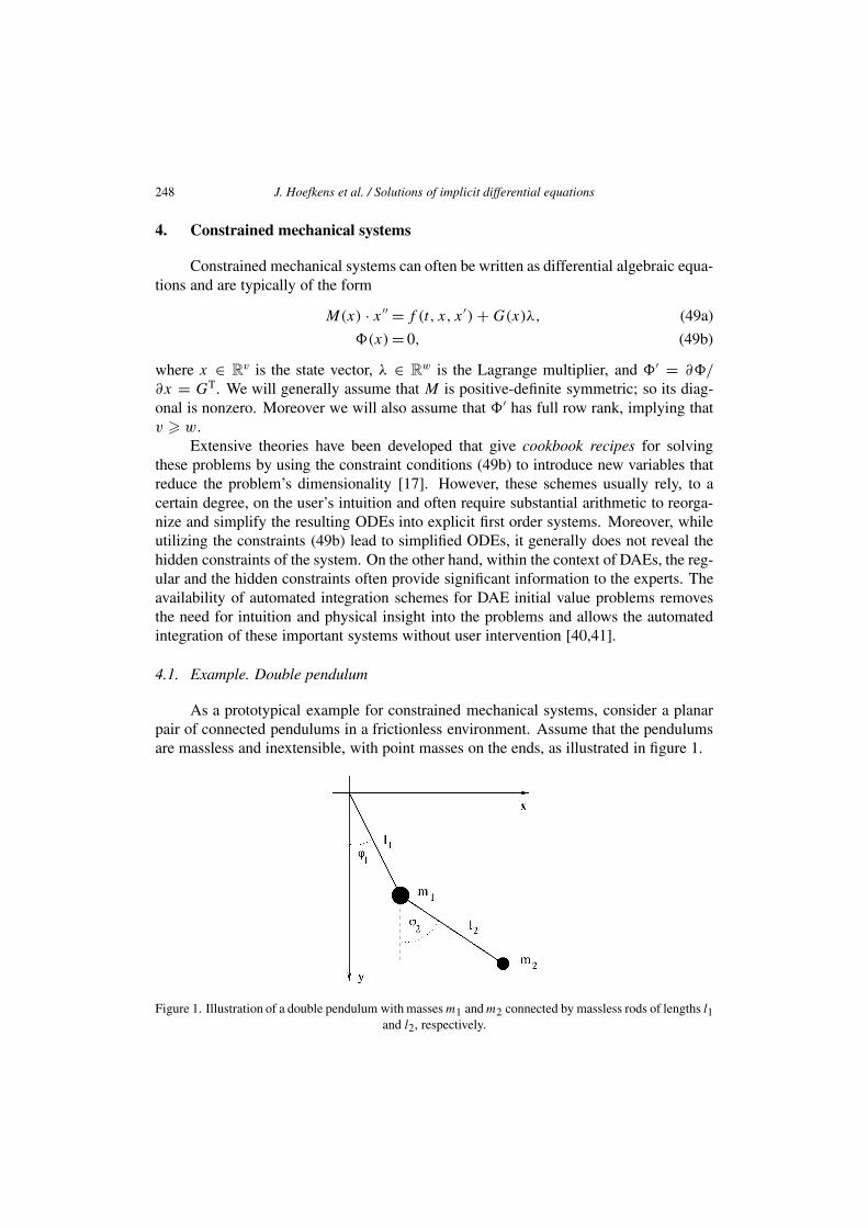
As a prototypical example for constrained mechanical systems, consider a planarpair of connected pendulums in a frictionless environment. Assume that the pendulumsare massless and inextensible, with point masses on the ends, as illustrated in figure 1.

Figure 1. Illustration of a double pendulum with masses m1 and m2 connected by massless rods of lengths l1and l2, respectively.


If we denote the tensions in the rods by λ1 and λ2, they take the roles of the La-grange multipliers in this problem and the equations of motion, expressed in the Carte-sian coordinates x1, y1, x2, y2, are given by

m1x′′1 + λ1x1

l1− λ2(x2 − x1)

l2= 0,

m2y′′1 + λ1y1

l1− λ2(y2 − y1)

l2− m1g = 0,

m2x′′2 + λ2(x2 − x1)

l2= 0,

m2y′′2 + λ2(y2 − y1)

l2− m2g = 0,

x21 + y2

1 − l21 = 0,

(x2 − x1)2 + (y2 − y1)

2 − l22 = 0.

(50)

While it is common practice in classical mechanics to reduce this problem to atwo-dimensional ODE in the angles ϕ1 and ϕ2, here the focus is on showing how ourmethod for the computation of self-validated DAEs can automatically treat this problemas an initial value problem in the six variables x1, y1, x2, y2, λ1 and λ2. By utilizing anexhaustive search and the Lζ test, our software correctly identifies the DAE as an index-2system and also determines that a solvable implicit ODE can be obtained by combiningthe first four equations of (50) with the second derivatives of the the algebraic constraints:

2(x′

12 + x1x

′′1 + y′

12 + y1y

′′1

) = 0,

2((x′

2 − x′1)

2 + (y′2 − y′

1)2 + (x2 − x1)(x

′′2 − x′′

1 ) + (y2 − y1)(y′′2 − y′′

1 )) = 0.

(51)

Starting with Taylor models describing the initial conditions y for ϕ1(0) =ϕ2(0) = 5◦, iterating the operator H finds the polynomial fixed point ζ(t, y):

ζ(t, y) = (ζ1, . . . , ζ6)(t, y) = H(ζ ) = (x′′1 , y

′′1 , x

′′2 , y

′′2 , λ1, λ2)(t, y). (52)

We construct a Taylor model T from the computed polynomial fixed point ζ , do-main intervals of ±0.001 (cf. table 2) and the remainder bound intervals listed in (53).[−0.107588 · 10−11, 0.107563 · 10−11

],

[−0.325530 · 10−12, 0.324108 · 10−12],[−0.827930 · 10−12, 0.827411 · 10−12

],

[−0.135636 · 10−11, 0.135024 · 10−11],[−0.586048 · 10−11, 0.586802 · 10−11

],

[−0.296806 · 10−11, 0.297409 · 10−11].

(53)


Table 2Taylor model describing the coordinate x1 after the first integration step (t = 0.001). Shown are thereference describing the dependence on the eight initial conditions (570 coefficients omitted), reference

points, domain intervals, and remainder bound.

RDA VARIABLE: NO= 7, NV= 8I COEFFICIENT ORDER EXPONENTS1 0.8715569933562087E-01 0 0 0 0 0 0 0 0 02 0.9999985208427887 1 1 0 0 0 0 0 0 0 0 03 0.1294094804033084E-06 1 0 1 0 0 0 0 0 04 0.4943135787532041E-06 1 0 0 1 0 0 0 0 05 -.4324683436783440E-07 1 0 0 0 1 0 0 0 06 0.9999995094698690E-03 1 0 0 0 0 1 0 0 07 0.4291582558871565E-10 1 0 0 0 0 0 1 0 08 0.1647712466901794E-09 1 0 0 0 0 0 0 1 09 -.1441561616042412E-10 1 0 0 0 0 0 0 0 1

10 0.3012457312051847E-06 2 2 0 0 0 0 0 0 011 0.4396925540227502E-06 2 1 1 0 0 0 0 0 012 -.4077392176614172E-07 2 0 2 0 0 0 0 0 013 0.2503569837970065E-12 2 1 0 1 0 0 0 0 014 0.4962017515784074E-06 2 0 1 1 0 0 0 0 0

...585 0.1432067646745945E-05 5 0 0 1 2 0 0 0 2586 -.1285873169976378E-06 5 0 0 0 3 0 0 0 2

VAR REFERENCE POINT DOMAIN INTERVAL1 0.8715574274765817E-001 [0.8615574274765816E-001,0.8815574274765817E-001]2 0.9961946980917455 [0.9951946980917455,0.9971946980917455 ]3 0.1743114854953163 [0.1733114854953163,0.1753114854953163 ]4 1.992389396183491 [ 1.991389396183491, 1.993389396183491 ]5 0.000000000000000 [-.1000000000000000E-002,0.1000000000000000E-002]6 0.000000000000000 [-.1000000000000000E-002,0.1000000000000000E-002]7 0.000000000000000 [-.1000000000000000E-002,0.1000000000000000E-002]8 0.000000000000000 [-.1000000000000000E-002,0.1000000000000000E-002]

REMAINDER BOUND INTERVALR [-.9116356403937544E-014,0.9118332138766990E-014]

The remainder bounds of H(T ) are shown in (54), and since the polynomials are fixedunder H, we prove the required inclusion H(T ) ⊂ T by comparing the remainderbounds of T (53) and H(T ) (54).

[−0.889002 · 10−12, 0.889003 · 10−12],

[−0.215533 · 10−12, 0.215533 · 10−12],[−0.550989 · 10−12, 0.550988 · 10−12

],

[−0.792687 · 10−12, 0.792689 · 10−12],[−0.544366 · 10−11, 0.544366 · 10−11

],

[−0.221796 · 10−11, 0.221795 · 10−11].

(54)

As a final illustration of the Taylor model approach and its ability to explicitlypropagate guaranteed enclosures of the functional dependence on initial conditions, ta-ble 2 lists parts of the final Taylor model for the solution x1(y) at the end of the firstintegration step at t = 0.001. The width of the remainder bound is less than 2 · 10−14,


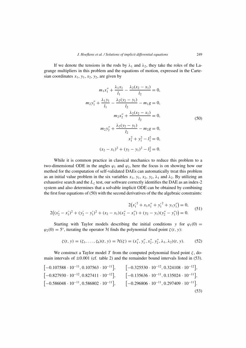
Figure 2. Coordinates x1 and x2 of the double pendulum for ϕ1(0) = ϕ2(0) = 5◦, 30◦, 90◦, x′1(0) =

x′2(0) = y′

1(0) = y′2(0) = 0 and 0 � t � 100 (g = 1, l1 = l2 = 1, m1 = m2 = 1).

providing an extremely tight enclosure of the solution and setting the stage for validatedlong-term integrations of differential algebraic equations.

Figure 2 illustrates the motion of the double pendulum by showing x1(t) and x2(t)

for various initial conditions over the time interval [0, 100]. The graphs highlight theoscillations of the system with an energy transfer between the two masses m1 and m2.While the system follows an almost periodic path for small energies, it shows signs ofchaotic motion for high energies.

Acknowledgements

We would like to thank John Pryce, Stephen Campbell, George Corliss, Ken Jack-son, Ned Nedialkov, and Clifford Weil for fruitful discussions on differential algebraicequations.

References

[1] U.M. Ascher and L.R. Petzold, Computer Methods for Ordinary Differential Equations andDifferential–Algebraic Equations (SIAM, Philadelphia, PA, 1998).

[2] M. Berz, Differential algebraic description of beam dynamics to very high orders, Particle Accelera-tors 24 (1989) 109.

[3] M. Berz, Forward algorithms for high orders and many variables, in: Automatic Differentiation ofAlgorithms: Theory, Implementation and Application (SIAM, Philadelphia, PA, 1991).

[4] M. Berz, Modern Map Methods in Particle Beam Physics (Academic Press, San Diego, 1999).[5] M. Berz, Constructive generation and verification of Lyapunov functions around fixed points of non-

linear dynamical systems, Internat. J. Comput. Res. (2001).[6] M. Berz, C. Bischof, G. Corliss and A. Griewank eds., Computational Differentiation: Techniques,

Applications, and Tools (SIAM, Philadelphia, PA, 1996).[7] M. Berz and J. Hoefkens, Verified high-order inversion of functional dependencies and superconver-

gent interval Newton methods, Reliable Computing 7(5) (2001) 379–398.


[8] M. Berz and G. Hoffstätter, Computation and application of Taylor polynomials with interval remain-der bounds, Reliable Computing 4(1) (1998) 83–97.

[9] M. Berz, G. Hoffstätter, W. Wan, K. Shamseddine and K. Makino, COSY INFINITY and its applica-tions to nonlinear dynamics, in: [6], pp. 363–365.

[10] M. Berz and K. Makino, Verified integration of ODEs and flows with differential algebraic methodson Taylor models, Reliable Computing 4(4) (1998) 361–369.

[11] M. Berz and K. Makino, COSY INFINITY version 8.1 reference manual, Technical Report MSUCL-1195, National Superconducting Cyclotron Laboratory, Michigan State University, East Lansing, MI48824 (2001).

[12] M. Berz, K. Makino and J. Hoefkens, Verified integration of dynamics in the Solar system, NonlinearAnal. 47 (2001) 179–190.

[13] K.E. Brenan, S.L. Campbell and L.R. Petzold, Numerical Solution of Initial-Value Problems inDifferential–Algebraic Equations (North-Holland, Amsterdam, 1989).

[14] Y.F. Chang and G.F. Corliss, Solving ordinary differential equations using Taylor series, ACM Trans.Math. Software 8 (1982) 114–144.

[15] Y.F. Chang and G.F. Corliss, ATOMFT: Solving ODEs and DAEs using Taylor series, Comput. Math.Appl. 28 (1994) 209–233.

[16] B. Erdélyi, J. Hoefkens and M. Berz, Rigorous lower bounds for the domains of definition of extendedgenerating functions, SIAM J. Appl. Dyn. Systems (2001) submitted.

[17] H. Goldstein, Classical Mechanics (Addison-Wesley, Reading, MA, 1980).[18] E. Griepentrog and R. März, Differential–Algebraic Equations and Their Numerical Treatment (Teub-

ner, Stuttgart, 1986).[19] E. Hairer and G. Wanner, Solving Ordinary Differential Equations II: Stiff and Differential–Algebraic

Problems (Springer, New York, 1991).[20] E.R. Hansen, Topics in Interval Analysis (Oxford Univ. Press, London, 1969).[21] J. Hoefkens, Rigorous numerical analysis with high-order Taylor models, Ph.D. thesis, Michigan State

University, East Lansing, MI (2001); also MSUCL-1217.[22] J. Hoefkens and M. Berz, Verification of invertibility of complicated functions over large domains,

Reliable Computing 8(1) (2002) 1–16.[23] J. Hoefkens, M. Berz and K. Makino, Efficient High-Order Methods for ODEs and DAEs (Springer,

New York, 2001) pp. 343–350.[24] J. Hoefkens, M. Berz and K. Makino, Verified High-Order Integration of DAEs and Higher-Order

ODEs (Kluwer Academic, Dordrecht, 2001) pp. 281–292.[25] R.B. Kearfott, Rigorous Global Search: Continuous Problems (Kluwer, Dordrecht, 1996).[26] E.R. Kolchin, Differential Algebraic Groups (Academic Press, New York, 1985).[27] R.J. Lohner, Enclosing the solutions of ordinary initial and boundary value problems, in: Computer

Arithmetic: Scientific Computation and Programming Languages, eds. E.W. Kaucher, U.W. Kulischand C. Ullrich, Wiley–Teubner Series in Computer Science (Teubner, Stuttgart, 1987) pp. 255–286.

[28] R. Lohner, Einschließung der Lösung gewöhnlicher Anfangs- und Randwertaufgaben und Anwen-dungen, Ph.D. thesis, Universität Karlsruhe (1988).

[29] K. Makino, Rigorous integration of maps and long-term stability, in: 1997 Particle Accelerator Conf.,Vol. 2, 1997, pp. 1336–1340.

[30] K. Makino, Rigorous analysis of nonlinear motion in particle accelerators, Ph.D. thesis, MichiganState University, East Lansing, MI, USA (1998); also MSUCL-1093.

[31] K. Makino and M. Berz, Remainder differential algebras and their applications, in: [6], pp. 63–74.[32] K. Makino and M. Berz, Efficient control of the dependency problem based on Taylor model methods,

Reliable Computing 5(1) (1999) 3–12.[33] K. Makino and M. Berz, Advances in verified integration of ODEs, in: SCAN’2000, 2000.[34] K. Makino and M. Berz, Global optimzation with Taylor models, Internat. J. Comput. Res. (2001).[35] K. Makino and M. Berz, Verified integration of transfer maps, Phys. Rev. ST-AB, submitted.


[36] R.E. Moore, Interval Analysis (Prentice-Hall, Englewood Cliffs, NJ, 1996).[37] R.E. Moore, Methods and Applications of Interval Analysis (SIAM, Philadelphia, PA, 1979).[38] N.S. Nedialkov, Computing rigorous bounds on the solution of an initial value problem for an ordinary

differential equation, Ph.D. thesis, University of Toronto (1999).[39] N.S. Nedialkov, K.R. Jackson and G.F. Corliss, Validated solutions of initial value problems for ordi-

nary differential equations, Appl. Math. Comput. 105(1) (1999) 21–68.[40] C.C. Pantelides, The consistent initialization of differential–algebraic systems, SIAM J. Sci. Statist.

Comput. 9(2) (1988) 213–231.[41] J.D. Pryce, A simple structural analysis method for DAEs, BIT 41(2) (2001) 364–394.[42] J.F. Ritt, Differential Equations from the Algebraic Viewpoint (Amer. Math. Soc., Washington, 1932).[43] J.F. Ritt, Integration in Finite Terms – Liouville’s Theory of Elementary Methods (Columbia Univ.

Press, New York, 1948).

Documents

Computing Validated Solutions of Implicit Differential Equations