Embed Size (px)
Citation preview
IOP PUBLISHING REPORTS ON PROGRESS IN PHYSICS
Rep. Prog. Phys. 76 (2013) 096801 (55pp) doi:10.1088/0034-4885/76/9/096801
On the genesis of the Earth’s magnetismPaul H Roberts1,3 and Eric M King2
1 Institute of Geophysics and Planetary Physics, University of California, Los Angeles, CA 90095, USA2 Earth and Planetary Science, University of California, Berkeley, CA 94720, USA
E-mail: [email protected]
Received 23 January 2011, in final form 26 June 2013Published 4 September 2013Online at stacks.iop.org/RoPP/76/096801
AbstractFew areas of geophysics are today progressing as rapidly as basic geomagnetism, which seeks tounderstand the origin of the Earth’s magnetism. Data about the present geomagnetic field pours infrom orbiting satellites, and supplements the ever growing body of information about the field inthe remote past, derived from the magnetism of rocks. The first of the three parts of this reviewsummarizes the available geomagnetic data and makes significant inferences about the large scalestructure of the geomagnetic field at the surface of the Earth’s electrically conducting fluid core,within which the field originates. In it, we recognize the first major obstacle to progress: because ofthe Earth’s mantle, only the broad, slowly varying features of the magnetic field within the core canbe directly observed. The second (and main) part of the review commences with the geodynamohypothesis: the geomagnetic field is induced by core flow as a self-excited dynamo. Itselectrodynamics define ‘kinematic dynamo theory’. Key processes involving the motion ofmagnetic field lines, their diffusion through the conducting fluid, and their reconnection aredescribed in detail. Four kinematic models are presented that are basic to a later section onsuccessful dynamo experiments. The fluid dynamics of the core is considered next, the fluid beingdriven into motion by buoyancy created by the cooling of the Earth from its primordial state. Theresulting flow is strongly affected by the rotation of the Earth and by the Lorentz force, which altersfluid motion by the interaction of the electric current and magnetic field. A section on‘magnetohydrodynamic (MHD) dynamo theory’ is devoted to this rotating magnetoconvection.Theoretical treatment of the MHD responsible for geomagnetism culminates with numericalsolutions of its governing equations. These simulations help overcome the first major obstacle toprogress, but quickly meet the second: the dynamics of Earth’s core are too complex, and operateacross time and length scales too broad to be captured by any single laboratory experiment, orresolved on present-day computers. The geophysical relevance of the experiments and simulationsis therefore called into question. Speculation about what may happen when computational power iseventually able to resolve core dynamics is given considerable attention. The final part of thereview is a postscript to the earlier sections. It reflects on the problems that geodynamo theory willhave to solve in the future, particularly those that core turbulence presents.
(Some figures may appear in colour only in the online journal)
Contents
1. Introduction 22. Description of the Earth’s magnetic field 4
2.1. Gauss decisively identifies an internalmagnetic origin 4
2.2. The power spectrum; the magnetic curtain 53. Time dependence 6
3.1. Historical secular variation 6
3.2. Archaeo- and paleomagnetism;paleomagnetic secular variation 8
4. The geodynamo hypothesis 105. Kinematic geodynamo theory 10
5.1. Pre-Maxwell electrodynamics 105.2. Extremes of Rm and finite Rm 135.3. Four successful kinematic models 155.4. Mean field electrodynamics 16
3 Author to whom any correspondence should be addressed.
0034-4885/13/096801+55$88.00 1 © 2013 IOP Publishing Ltd Printed in the UK & the USA

Rep. Prog. Phys. 76 (2013) 096801 P H Roberts and E M King
6. MHD geodynamo theory 186.1. The cooling Earth model 186.2. A simplified cooling Earth model 226.3. Rotational dominance; Proudman–Taylor
theorem; CMHD 256.4. Convection of small and finite amplitude 28
7. Numerical simulations 337.1. Numerical methods 337.2. Dynamo mechanisms 337.3. Dynamo regimes 357.4. Reversals; boundary conditions 367.5. Inner core rotation 37
7.6. Scaling 387.7. Taylorization and hints of magnetostrophy 41
8. Laboratory experiments 418.1. Dynamo experiments 428.2. Core flow experiments 44
9. The future 459.1. Computational progress and limitations 459.2. Turbulence 47
10. Overview 50Acknowledgments 51References 51
1. Introduction
In his encyclopedia, Pliny the elder told a story about ashepherd in northern Greece who was astonished to find thathis iron-tipped staff and the nails in his shoes were stronglyattracted to a rock, now called lodestone. His name, Magnes,possibly led to the phenomenon he experienced being called‘magnetism’.
The directional property of the magnetic compass needlewas apparently discovered, perhaps thousands of years ago,in China. It is certain that, from about the third century AD83 onwards, Chinese geomancers knew that a spoon, made oflodestone spun on a smooth horizontal surface, would cometo rest pointing in a unique southerly direction, which was notprecisely south. The deviation is today called declination andis denoted by D.
That magnetism can be acquired by iron by stroking itwith lodestone was an important though undated discoverythat led to the magnetic compass, first mentioned by ShenKua in 1088, a century before the first European referenceby Alexander Neckham of St Albans England in 1190. Bythe fourteenth century the nautical compass was in regular useby the British navy. Christopher Columbus carried one on hisepic voyage of 1492. By this time, a portable sundial couldbe easily purchased whose gnomen could be orientated by amagnetic compass needle beneath a window in its base. In1581 Robert Norman, an instrument maker in London, reportedthat a magnetized needle that was freely suspended, instead ofbeing pivoted about a vertical axis, orientates itself at a steepangle to the horizontal plane. This angle is called inclinationand denoted by I .
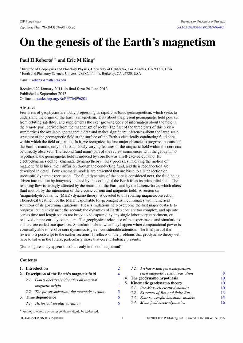
At first many thought the magnetism of the Earth wascreated externally, by attraction to the pole star. The discoverythat it originates mainly inside the Earth is often attributedto William Gilbert, court physician of Queen Elizabeth 1stof England, who in 1600 published De Magnete, a book thatsoon became famous and is often called ‘the first scientifictextbook’. He there describes his ‘terrella’, or little Earth,experiment, in which he placed the points of iron pins onthe surface of a spherical block of lodestone (or magneticrock), and found that they became orientated at different pointson the surface in ways similar to the directions in which afreely suspended magnetic compass needle points at differentlocations on the Earth’s surface; see figure 1. ‘The Earth is agreat magnet’, he announced. Petrus Peregrinus de Maricourt
had previously, in a letter written in 1269, partially anticipatedGilbert. He had constructed his own terrella and, by laying aneedle on its surface, had mapped out the lines of magneticlongitude, finding them to be approximately great circlesconverging at two antipodal points which, in analogy with theEarth, he called poles. With the help of other magnets, heestablished that like poles repel and unlike poles attract.
Gilbert believed that the Earth is magnetically modeledso well by his terrella that its magnetism is time independenttoo, but in 1635 Henry Gellibrand produced convincingobservational evidence that contradicted this. Timedependence is the very significant topic of section 3. Sincepermanent magnets creating constant magnetic fields werethe only sources of magnetism that were known at that time,it was natural to suppose that the Earth’s magnetic field isproduced by moving magnetic poles within the Earth. Halley,of comet fame, who in 1701 had produced a famous map ofD in the Atlantic, visualized four magnetic poles moving in ahollow Earth, but that did not explain the observational factswell. The situation was, from 1635 until almost a century ago,frustratingly mysterious. As Christopher Hansteen eloquentlycomplained in 1819, ‘The mathematicians of Europe since thetimes of Kepler and Newton have all turned their eyes to theheavens, to follow the planets in their finest motions and mutualperturbations: it is now to be wished that for a time they wouldturn their gaze downwards towards the earth’s center, wherealso there are marvels to be seen; the earth speaks of its internalmovements through the silent voice of the magnetic needle’(Chapman and Bartels 1940). In defense of mathematicians,it must be admitted that what they could do in 1819 was verylimited; the Earth’s core was not discovered until 1906 byRichard Dixon Oldham. That it was fluid was not known forcertain until two decades later.
The first mathematician to take up Hansteen’s challengewas Karl Friedrich Gauss who, in 1838 in an analysisdescribed in section 2, gave Gilbert’s idea mathematicalteeth. But it still left geomagnetism without an adequatephysical explanation. This came only after the birth ofelectromagnetism. Allessandro Volta discovered in 1800how to construct what became known as a voltaic pile, fromwhich electric current could be carried along an electricallyconducting wire. In 1820, Hans Christian Oersted showed thatthe needle of a compass placed near a wire carrying an electriccurrent was deflected. News quickly reached Paris where, inthe same year, Francois Arago demonstrated that the magnetic
2
Rep. Prog. Phys. 76 (2013) 096801 P H Roberts and E M King
Figure 1. A sketch of William Gilbert’s terrella from De Magnete(1600). From Chapman and Bartels (1940), with permission fromOUP.
field produced by the current was as capable of magnetizingiron as a permanent magnet. Also in 1820, Jean-Baptise Biotand Felix Savart published their well-known law relating alinear current to its magnetic effect. In 1825, Andre-MarieAmpere published his famous memoir that led to what is nowcalled Ampere’s law: ∇×H = J , where J is the electriccurrent density in A m−2 and H (A m−1) is the magnetizingforce (aka ‘magnetic intensity’); A stands for amp.
Not only was electromagnetic (EM) theory taking shapebut also an alternative origin of geomagnetism had beenidentified: the flow of electric current inside the Earth!The time dependence of the magnetic field discovered byGellibrand prompts a reminder of Michael Faraday. Foremostamongst his prodigious achievements was the discovery of thelaw of EM induction, which relates the time derivative of themagnetic field, B (aka ‘magnetic induction’), to the electricfield E:
∇×E = −∂tB, consistent with ∇ · B = 0, (1a, b)
the latter of which is sometimes called ‘Gauss’s law’. Themagnetic field B is in tesla (T) and the electric field in volts permeter (V m−1). Faraday also introduced the concept of linesand tubes of (magnetic) force, which will be useful below.
A permanently magnetised material loses its magnetism ifheated beyond the Curie temperature. Except in its outermostlayers called ‘the crust’, the Earth is so hot that magnetism canonly be the by-product of electric current flow. In other words,B and H are essentially the same but, in the SI units used here,even their physical dimensions are different! The constant ofproportionality, µ, in the law B = µH is the permeability,with physical dimensions henry per meter (H m−1, whereH = T m2 A−1). It appears that, in the Earth, µ is almostthe same as µ0, the permeability of free space, which in SIunits is µ0 = 4π × 10−7H m−1 (precisely!). Ampere’s lawbecomes
∇×B = µ0J, so that ∇ · J = 0. (2a, b)
Equations (1a, b) and (2a) are three of the ‘pre-Maxwellequations’, so called because they pre-date those of JamesClerk Maxwell, who introduced a displacement current toresolve the inconsistency of (2b) with charge conservation,which requires ∂tϑ + ∇ · J = 0, where ϑ is charge density inC (coulomb = A s). Light could cross the Earth’s diameterin about 40 µs, or in effect instantaneously in comparisonwith the time scales of the geomagnetic phenomena consideredbelow, which are 1 day and longer. Therefore both ∂tϑ anddisplacement currents are negligible, leading to pre-Maxwelltheory in which light has infinite speed, and the electric fieldenergy is negligible compared with the magnetic.
Pre-Maxwell electrodynamics are closed by Ohm’s lawwhich, for a conductor moving with a velocity u much lessthan light speed, is
J = σ(E + u×B), (3)
where σ (in siemens per m) is the electrical conductivity. Apartfrom boundary conditions, all the electrodynamics needed inthis article have now been assembled.
In 1919, Joseph Larmor made the dynamo hypothesis,according to which the electric currents responsible for themagnetic fields of the Earth and Sun are created in much thesame way as by electric generators in power stations. In thefirst dynamos, made in the early 19th century, electric currentwas created inductively by the rotation of current-carrying coilsin the presence of the magnetic field of fixed permanent mag-nets. In 1854 Ernst Werner Siemens invented the self-exciteddynamo, in which the inducing magnetic field is instead pro-duced by fixed current-carrying coils fed by the machine itself.This self-excited dynamo was what Larmor envisaged, and itis the only explanation of geomagnetism seriously entertainedtoday. We next assemble relevant geophysical facts.
To within a factor of 1/300, the Earth is a spherical bodyof radius a = 20 000/π km (by the original definition of themeter). Its internal structure is revealed by seismology, thestudy of acoustic waves generated by earthquakes. The wavestravel through the Earth and emerge loaded with information.They reveal the density of the material they pass through,and the velocities of the longitudinal and transverse acousticwaves, called P and S waves. Since the Earth is close tobeing spherically symmetric, these quantities are functions ofr alone, the distance from the geocenter O. See for examplethe PREM model of Dziewonski and Anderson (1981) or theak135 model of Kennett et al (1995). Seismology reveals thatinternally, the Earth consists of a rocky mantle lying above adense core whose surface is the core–mantle boundary (CMB),of radius ro = 3480 km. The core has two major parts: theinner core is a solid sphere of radius ri = 1225 km whosesurface is the inner core boundary (ICB). The outer core isthe annular region between the ICB and CMB and is knownto be fluid because only P waves pass through it. Atop theuppermost mantle is the crust. See figure 2.
The seismically inferred density of Earth’s core, combinedwith projections of Earth’s relative chemical abundances basedon chemical makeup of meteorites from which it likely formed,suggest that Earth’s core is mostly iron. (About 8% of the coremay be nickel but, since the physical properties of these two
3

Rep. Prog. Phys. 76 (2013) 096801 P H Roberts and E M King
Figure 2. The gross structure of Earth’s deep interior.
metals are much alike, this is neither easy to determine norimportant for the geodynamo.) The density of the core is,however, a few percent less than that expected of pure iron.The generally accepted interpretation is that both cores aremixtures of iron and a few percent lighter chemical elements,but seismology cannot identify these. Being iron-rich themixtures should be good conductors of electricity, unlike therocky mantle and crust. The variation of density ρ(r) andpressure P(r) in the fluid core is consistent with the idea thatit is well mixed by the internal motions, u.
Our review has three main parts. Part 1, made up ofsections 2 and 3, assembles relevant observational data andinterpretations. Section 2 explains how the geomagnetic fieldis best represented and interpreted, and section 3 reports on itstime dependence.
Part 2 describes how theory (sections 4–6), computersimulations (section 7), and experiments (section 8) haveadvanced understanding of geomagnetism to where it is today.Section 4 discusses the geodynamo hypothesis, which framesall that follows. Section 5 formulates the dynamo problemwith pre-Maxwell electrodynamics. In it we address howkinetic energy is converted to magnetic energy in a topic calledkinematic dynamo theory. Section 6 presents governing MHDequations for the geodynamo and discusses the fluid dynamicsof Earth’s core.
Part 3, consisting of sections 9 and 10, points to thefuture, where the deficiencies that still exist will ultimatelybe resolved. Section 9 discusses turbulence, a substantialobstacle in understanding natural fluid systems. It maybe fundamentally important for core dynamics and thegeodynamo. Section 10 concludes our presentation.
A few remarks about notation may be helpful: ‘Conduc-tivity’ and ‘diffusivity’ stand for ‘electrical conductivity’ and‘magnetic diffusivity’ unless ‘thermal’ is added. ‘Magneticfield’ is abbreviated to ‘field’ and ‘electric current density’ to‘current’. Unit vectors are not decorated with a circumflex,which is used instead to distinguish fields belonging to the ex-terior of the core (mantle, crust and beyond); unit vectors aredenoted by a bold unity, 1.
PART 1: Magnetic observations
2. Description of the Earth’s magnetic field
2.1. Gauss decisively identifies an internal magnetic origin
Gilbert’s belief that the source of the Earth’s magnetismis within it was confirmed by Gauss in 1838 through anapplication of potential theory. Assuming negligible currentflow J = 0 at the Earth’s surface r = a, (1b), and (2a) showthat the magnetic field B at r = a satisfies
∇×B = 0, ∇ · B = 0. (4a, b)
Here, ‘hatted’ terms indicate quantities outside the fluid outercore. Equations (4a, b) shows that B is a potential field forwhich
B = −∇V, where ∇2V = 0, (4c, d)
and V is the geopotential. In terms of spherical coordinates(r , θ , φ), where θ is colatitude (i.e. 1
2π -latitude) and φ is eastlongitude, the spherical components of (4c) are
Br = −∂V
∂r, Bθ = −1
r
∂V
∂θ, Bφ = −1
s
∂V
∂φ,
(4e, f, g)
where s = r sin θ . The components (4e–g) are three of themagnetic elements, and are usually denoted by −Z, −X andY , respectively. Others are the declination, D = tan−1(Y/X)
and the inclination, I = tan−1(Z/H), where H = √(X2 +Y 2)
is the horizontal field strength; the total field strength isF = √
(X2 + Y 2 + Z2). Of particular interest to marinershas been D, which is the eastward deviation of the (magnetic)compass needle from true North; I is the downward dip of afreely suspended compass needle to the horizontal.
The general solution of (4d) is
V (r, θ, φ, t) = Vint(r, θ, φ, t) + Vext(r, θ, φ, t), (5a)
where
Vint(r, θ, φ, t) = a
∞∑=1
(a
r
)+1
×∑
m=0
[gm (t) cosmφ + hm
(t) sin mφ]Pm (θ), (5b)
Vext(r, θ, φ, t) = a
∞∑=1
( r
a
)
×∑
m=0
[gm (t) cosmφ + hm
(t) sin mφ]Pm (θ), (5c)
4

Rep. Prog. Phys. 76 (2013) 096801 P H Roberts and E M King
and Pm (θ) is the Legendre function of degree and order
m. In these expansions, gm , hm
, gm and hm
are calledgauss coefficients. (The Legendre functions are ‘Schmidtnormalized’, an option not much used outside geophysics.The mean square over the unit sphere of Pm
(θ) cosmφ andof Pm
(θ) sin mφ is (2 + 1)−1.)The potential Vint(r, θ, φ, t) represents the field created
by sources below the Earth’s surface. In (5b), it is expressedthrough multipoles at the geocenter, O, the monopole ( = 0)being excluded. The g0
1 term gives the (centered) axial dipole,while g1
1 and h11 determine the (centered) equatorial dipole.
Since the units of B are tesla (T), the components of the dipolemoment are obtained in T m3 by multiplying g1
1, h11 and g0
1 by4πa3. The dipole moment, m, of the Earth is, however, usuallyexpressed in A m2, so the field of the central dipole is
Bd(r) = 1
f0
(a
r
)3[3(m · 1r )1r − m],
where m = f0(g111x + h1
11y + g011z), (6a, b)
f0 = 4πa3/µ0 ≈ 2.580 × 1027 m4 H−1 and 1r = r/r; seesection 1. The strength of the central dipole is m = f0[(g0
1)2 +
(g11)
2 + (h11)
2]1/2 and is currently about 7.8 × 10²² A m2 anddecreasing. The coefficients g0
2 , g12, h1
2, g22 and h2
2 correspondto quadrupoles at O, g0
3 , g13, h1
3, g23 , h2
3, g33 and h3
3 to octupoles,etc. The larger the , the more rapidly does that part to Vint
increase with depth.The potential Vext(r, θ, φ, t) represents the field created
by sources above the Earth’s surface, such as currents flowingin the ionosphere. The leading terms, g0
1 , g11 and h1
1, in (5a),give uniform fields in the z-, x- and y-directions, The largerthe , the more rapidly does its contribution to Vext increasewith r . Further details about the harmonic expansions can befound in many places, including Chapman and Bartels (1940)and Langel (1987).
In 1838, Gauss published the first spherical harmonicanalysis of the geomagnetic field. From data available to him,he interpolated for X, Y and Z at 84 points, spaced 30 inlongitude on 7 circles of latitude. He assumed that Vext = 0and truncated (5b) at N = 4:
V (r, θ, φ, t) = a
N∑=1
(a
r
)+1
×∑
m=0
[gm (t) cosmφ + hm
(t) sin mφ]Pm (θ). (7)
Without any computational aid for the considerable arithmeticlabour involved, he extracted the 24 g and h coefficients.(According to the usual mantra, he avoided aliasing, because84 points >3×(24 gauss coefficients) = 72.) He then testedhow well (7) fitted the data at the 84 points, and concludedfrom the excellence of the fit that Vext was in fact small enoughto be ignored. Subsequent analyses, drawing of much largerdata sets, have confirmed the smallness of Vext and electroniccomputers have made (7) readily accessible for large N .
2.2. The power spectrum; the magnetic curtain
From now on we accept that the main source of the magnetismof the Earth lies entirely beneath its surface, so that (7) holds
0 3 6 9 12 15 18 21 24 27 3010-12
10-9
10-6
10-3
100
103
106
(mT
2 )
CMB field
R
mag
netic
curt
ain
surface field
Figure 3. A Mauersberger–Lowes spectrum for geomagnetic fieldintensity as a function of harmonic degree; see (8a). Gausscoefficients for data points are taken from the xCHAOS model ofOlsen and Mandea (2008), derived from field measurements fromsatellite and ground-based observatories made between 1999 and2007. Hollow symbols show the spectrum at Earth’s surface, R(a);solid symbols show it at the CMB, R(ro). The shading illustrateswhere information about the core is hidden behind the magneticcurtain, the edge of which is indicated.
exactly. We denote by B(x, t) the field created by the 2 + 1harmonics of degree . Its mean square over the sphere ofradius r , which we denote by S(r), is R(r, t). This is thepower spectrum of Mauersberger (1956) and Lowes (1966),which we call the ‘ML-spectrum’:
R(r, t) =(a
r
)2+4( + 1)
∑m=0
[(gm (t))2 + (hm
(t))2]
and 〈B2(r, t)〉 =∞∑=1
R(r, t). (8a, b)
The ML-spectrum for Earth’s surface field, R(a, t), is shownin figure 3 as hollow symbols. Surface field power decreasessteadily until about = 13, above which the spectrum flattens.Assuming there are no magnetic sources in the mantle, we canproject this surface ML-spectrum to the CMB by multiplyingR(a, t) by (a/ro)
2+4 = 11.2(3.35). This factor tips thespectrum up, the result of which is shown as solid symbols infigure 3. The CMB spectrum is nearly flat up to = 13, abovewhich the power increases with .
The ML-spectrum for 13 and 13 are generatedby different processes. The large scale observed field, 13,is the main geodynamo field produced in the core. The fieldmeasured on smaller scales, 13, however, is due to crustalmagnetism. The Curie temperature of mantle materials istypically in the range 300–1000 C. These temperatures arereached within tens of kilometers of Earth’s surface, so thatthe crust can be at least partially magnetized. The excessiveamount of power attributed to the small-scale CMB field inthe upper curve of figure 3 is unphysical, since ferromagneticsources in the mantle render (4c, d) and (7) invalid belowr = a. We have therefore incorrectly extrapolated a localsource of magnetism to a more distant origin, artificiallyamplifying its intensity. Instead, we observe distinct spectral
5

Rep. Prog. Phys. 76 (2013) 096801 P H Roberts and E M King
behaviors of core and crust, R<13 and R>13, which are bothnearly flat at their sources, r = ro and r = a, respectively. Thisobservation led Hide (1978) to suggest that a lower bound forthe radius of a conducting planetary core could be derivedfrom magnetometers on orbiting satellites by assuming thespectrum, R(r), at its core surface is perfectly flat. Elphicand Russell (1978) quickly applied the idea to Jupiter. Testedfor the Earth, Hide’s idea gives 3310 km as a lower bound forthe core radius. The physical reason why the spectrum shouldbe so flat (or ‘white’) at the surface of a conducting core isuncertain.
The ML-spectrum is not completely flat at the CMB for < 13; the dipole = 1 predominates. The interestingquestion of whether this is invariably true has been answeredin the negative by the study of paleomagnetism; see section 3.1.Also numerical models (section 7) have different spectralcontent. This has led to the introduction of a parameter calleddipolarity (Christensen and Aubert, 2006), defined by
d(N) =( ∫
CMB B2=1d2x∫
CMB
∑N=1 B2
d2x
)1/2
=(
R1(ro)∑N=1 R(ro)
)1/2
.
(8c)
If R(ro) were perfectly flat for 1 N , this would beN−1/2, so that d(12) ≈ 0.29; in reality, today’s geomagneticfield features a prominent dipole term, and d(12) = 0.68.
Crustal magnetism influences the study of Earth’smagnetic field in two fundamental ways. First, the magnetismof ancient crust provides valuable geomagnetic informationcovering much of Earth’s history, a topic raised in section 3.2.Second, crustal magnetism forms a magnetic curtain, whichoccludes a view of the core field for all but its largestscales. Gauss coefficients measured at Earth’s surface areoverwhelmed by crustal sources for > max ≈ 13, limitingmain field observations to length scales larger than
L = 2πro/max ≈ 1.7 × 10³ km. (8d)
Detailed knowledge of the deep field is hidden behind themagnetic curtain.
The extent to which the magnetic curtain is detrimental toknowledge of the geomagnetic field at its source is illustratedin figure 4, which shows the radial magnetic field of Earth(top row) and a numerical geodynamo simulation (middleand bottom rows) at the surface (left column) and CMB(right column). Numerical simulations are not veiled by anymagnetic curtain, and so the full spectrum (within numericalresolution) is visible at the CMB. This full-spectrum fieldis shown in the bottom row of figure 4, which illustratesthat, although the surface field is not strongly affected, theinclusion of higher order terms produces a CMB field mapthat is substantially different from the truncated version. Thisshows how drastically the magnetic curtain limits observationsof Earth’s field at its source.
So far time, t , has been carried along in the analysis but hashad no part in it. The time dependence of B, the focus of thenext section, induces currents and fields within the mantle andcrust, because they are not perfect electrical insulators. Time-varying B on the CMB induces electric currents, particularly
At surface At core-mantle boundary
Geomagnetic field (IGRF-11) up to degree 13
Simulation plotted up to degree 13
Simulation plotted up to degree 213
Figure 4. Radial field at the surface (left column) and CMB (rightcolumn) of Earth for 13 (top row), a numerical geodynamosimulation for 13 (middle row), and the same simulation for 213 (bottom row). Figure courtesy of K M Soderlund.Geomagnetic data taken from the International GeomagneticReference Field (IRGF-11, Finlay et al 2010b).
in the lower mantle, that shield the CMB from observationat the Earth’s surface if |∂tB| = O(|B|/τ) exceeds |B|/τσ |,where
τσ =(∫ a
ro
(µ0σ (r))1/2dr
)2
, (9)
and σ (r) is the mantle conductivity, which is poorly known inthe lower mantle where it is largest and matters most. Estimatesof τσ of about 1 yr are common; see Backus (1983). Mantleconduction is rarely of interest in the topics reviewed here, butit is touched on in sections 5.1.4 and 6.3.3. Elsewhere it isassumed that σ ≡ 0 so that τσ = 0.
In summary, this section has shown that the magneticcurtain permits observation of only the largest (L > L) andslowest (τ > τσ ) field variations at the CMB, for which thepotential field of section 2.1 applies above the CMB.
3. Time dependence
3.1. Historical secular variation
Earth’s field varies on a vast range of time scales. Changeson time scales of years to centuries are part of what is calledthe (geomagnetic) secular variation or (G)SV. Much longertimes are studied today, and the use of ‘secular’, as meaningenduring over a long period of time, is an anachronism. TheGSV has been directly measured and recorded for the past fourcenturies, owing mostly to the importance of D for maritimenavigation (Jackson et al 2000). Part of the GSV that attractedearly and lasting attention is the westward drift of magneticfeatures, particularly isolines of Y and D near Europe. Thedrift is far from uniform and not entirely westward. Ten
6

Rep. Prog. Phys. 76 (2013) 096801 P H Roberts and E M King
CMB Secular Variation
mT
/yr
−0.01
0
0.01CMB Field
mT
−0.8
0
0.8
Surface Secular Variation
mT
/yr
−1
0
1x 10
−4Surface Field
mT
−0.08
0
0.08
Figure 5. Radial magnetic field Br (left panels) and secular variation ∂t Br (right panels) at Earth’s surface (top panels) and the CMB(bottom panels). Data from observations in 2004 are taken from the xCHAOS model of Olsen and Mandea (2008) for 13.
different ways of analyzing it are given in section 12.3 ofLangel (1987). Whether it is a permanent feature of the fieldis unknown and sometimes doubted. As even its reality orotherwise is inessential for this article, we ignore it below,except in section 7.5.
Information about the time dependence of D, I and F
has been gathered in historical times mainly in the past 4, 3and 2 centuries, respectively; it is called the historical secularvariation (HSV) (Jackson et al 2000). During this time, thefield has been dipole dominated, with a moment, m, that hasdecreased at a rate of about 5% per century, which is fasterthan the natural diffusive decay rate; see section 5.2.1. Also,several small abrupt changes, called ‘geomagnetic impulses’or ‘jerks’, have occurred on a worldwide basis. The origins ofthese are unknown. We ignore them here, but see Courtillotand LeMouel (1984), Mandea et al (2010).
Today, the Earth’s field is constantly monitored by a globalarray of ground based observatories and dedicated satellites.Figure 5 shows an example of such measurements, taken fromthe xCHAOS model of Olsen and Mandea (2008). The leftpanels are maps of Earth’s radial field Br at the surface (r = a)and CMB (r = ro). The right panels show secular variation as∂t Br for the surface and CMB. If the magnetic curtain couldbe pierced, the lower panels would show much greater detailfrom the high harmonics; see figure 4.
Such maps of secular variation are made possible bymeasurements of the time derivatives, gm
and hm , of the Gauss
coefficients. These measurements also permit analysis of thespectra of secular variation which, in analogy with (8a), isdefined as
A(r, t) =(a
r
)2+4( + 1)
∑m=0
[(gm (t))2 + (hm
(t))2] (10a)
(Lowes 1974). From this spectrum, a characteristic time scalecan be derived for each harmonic , sometimes called its
0 1 2 3 4 5 6 7 8 9 10 11 12 13 141015
1018
1021
1024
1027
Ene
rgy
(J)
Kinetic Energy
Magnetic Energy
Figure 6. Estimates of magnetic (circles) and kinetic (squares)energy spectra for 13 at the surface of Earth’s core,using (10d, e).
correlation time (Stacey 1992):
τ cor =
(R
A
)1/2
=(∑
m=0[(gm (t))2 + (hm
(t))2]∑
m=0[(gm (t))2 + (hm
(t))2]
)1/2
.
(10b)
If changes in the large scale field at the CMB are directly relatedto flow there, the speed of such flow for each can be crudelyestimated as
U = 2πro/ τcor , (10c)
which leads to estimates of the core’s magnetic and kineticenergy spectra:
M = 1
2µ0R(ro)Vo and K = 1
2MoU2
, (10d, e)
where Vo (≈ 1.77 × 10²⁰ m3) is the volume of the core andMo (≈1.8 × 1024 kg) is its mass. See figure 6. As (10d, e)
7

Rep. Prog. Phys. 76 (2013) 096801 P H Roberts and E M King
Figure 7. A core flow inversion map from Holme and Olsen (2006),with permission. The inversion assumes frozen flux and tangentialgeostrophy; see section 5.2.1 and Finlay et al (2010a).
are derived only from B and ∂tB at the CMB, they should beregarded as preliminary estimates.
High resolution satellite data are used to reconstructcore surface flow, U(θ, φ, t), from the secular variation ofthe vertical field, Z(ro, θ, φ, t), obtained by extrapolatingZ(a, θ, φ, t) downwards, as described in section 2.2. Thetechnique is based on the frozen flux approximation (FFA),which will be described in section 5.2.1. Here we note onlythat u = 0 on the CMB by the so-called ‘no-slip’ condition,and that the FFA seeks u at r = r−
o , i.e. just beneath a thinboundary layer on the CMB. Although ur = 0 on r = ro,there are upwellings and downwellings from r = r−
o into andout of the boundary layer so that ∇ · u does not vanish atr − r−
o . The FFA assumes that fast, large scale motions of anelectrical conductor will sweep field lines along as unresistingpassengers (field lines being defined as curves parallel tothe instantaneous B). This approximation relates Z(ro, t)
to u at r = r−o , i.e. U(θ, φ, t). Since however U has two
non-zero (tangential) components but Z(ro, t) has only one,an additional assumption is required to determine U . Severalhave been proposed, some of which add dynamical ingredients.The results of such SV inversions are maps of U , one ofwhich is shown in figure 7. Different inversion methods leadto different U and to disputes about the merits of differentinversion methods. These disputes are difficult to resolve inpart due to limitations imposed by the magnetic curtain. Themagnitude of core flow near the CMB is typically found (Finlayand Amit 2011) to be about
U = 4 × 10⁻⁴ m s−1 and τO = ro/U = 200 yr
(10f, g)
will be taken as characteristic of fluid circulations in thecore, an eddy overturning time. The observationally inferredestimate (10f ) for the typical magnitude of core flow willbe used everywhere below and, importantly, is in principlesufficient for magnetic field generation (see section 5.1.1).
3.2. Archaeo- and paleomagnetism; paleomagnetic secularvariation
Geological processes continuously create new material and,thanks to minerals it may contain such as magnetite, it maypreserve a magnetic record of its birth. The importance of
this record was fully recognized in the 20th century, and led tosome of the most striking advances in the whole of geology andgeophysics. These have benefitted from the greatly improveddating of materials through their radioactive content.
Arch(a)eomagnetism is the branch of archaeology thatstudies the magnetic field retained by ancient manmadeobjects at the time they were created. (See Gubbins andHerrero-Bervera 2007.) Paleomagnetism seeks to find andinterpret the magnetism acquired by rocks at birth but, becausethis may change subsequently for a myriad of reasons, anothersubject, called rock magnetism, is intimately involved. Thisstudies processes that modify the magnetization of rocks. Wedo not discuss archaeomagnetism and rock magnetism below.
Paleomagnetism may be divided into the magnetism ofigneous rocks such as lavas, and of sedimentary material suchas deposits at the bottom of lakes and oceans. Igneous rocksacquire their magnetization as they cool through the Curiepoints of the magnetic minerals they contain. Sedimentsbecome magnetized while in solution as the magnetic grainsthey contain orientate themselves parallel to the prevailingfield; they remain orientated after settling and becomingfixed in the sediment. Each approach has its strengths andlimitations, which need not be described in detail here, thoughwe give a few examples. As volcanic eruptions are sporadic,igneous rocks never provide a continuous record. Theirmagnetization is, however, stronger than that of sedimentaryrocks, from which absolute intensities, F , cannot be easilyextracted. A sediment from an ocean core can however giverelative intensities at different depths, and these correspond todifferent geological ages.
Turning now to the spectacular successes ofpaleomagnetism, one thinks first of continental drift, polarwandering, Pangea B and all the striking geological informa-tion that has emerged, but these topics are scarcely relevanthere. We confine ourselves to the very impressive discoveriesabout the paleomagnetic secular variation (PSV), the behaviorof the magnetic field over geologic time. The subject deservesmore space than we can give it. Readers might enjoy the en-tertaining book by Glen (1982). Many publications describein detail how data is evaluated and interpreted. See for exam-ple Merrill et al (1996) and numerous papers in Kono (2006)and Gubbins and Herrero-Bervera (2007). The character ofthe PSV may be summarized as follows:
1. VGP; VDM; paleomagnetic poles. Data taken from asingle site may be conveniently re-expressed in terms ofthe dipole moment, m, of a single geocentric dipole. Apoint where the axis of this dipole meets the Earth’s surfaceis called a virtual geomagnetic pole (VGP). It is virtualbecause it is derived on the assumption that only the = 1terms are present in (7). Because of the missing harmonicsfor other , the VGP is a function of site location. Thisis also true of the magnitude |m| of m, which is calledthe virtual dipole moment (VDM) and can be determinedonly if F is available at the site. The VGP and VDMdepend not only on site but also on time, through the PSV.This fluctuation in the VGP may be removed by takingthe local time average, over a period of 104–105 yr. The
8

Rep. Prog. Phys. 76 (2013) 096801 P H Roberts and E M King
Figure 8. Time-averaged CMB field over 0–0.5 Myr from lava andsedimentary data (Johnson and Constable 1997). This material isadapted from Johnson et al (2008) with permission from JohnWiley & Sons, Inc. Copyright 2008.
60
65
70
75
80
85
90
95
100
105
110
115
120
0
5
10
15
20
25
30
35
40
45
50
55
60
120
125
130
135
140
145
150
155
160
165
170
175
180
mill
ion
year
s be
fore
pre
sent
Figure 9. A timeline of geomagnetic polarity reversal occurrences.Data extracted from Kent and Gradstein (1986).
result is called the paleomagnetic pole and is the focus ofmost paleomagnetic research.A significant way of interpreting paleomagnetic polepositions is suggested by figure 8, which is Br at theCMB, averaged over the last 0.5 Myr. The result isdominantly that of an axial dipole, with its axis parallelto the current direction of the Earth’s angular velocity,Ω. This idea led to the geocentric axial dipole hypothesis(GAD hypothesis), which asserts that the average of B
over a period of order 104–105 yr is the field (6a) of anaxial dipole, m = m(t)1z′ , where m(t) is the virtual dipolemoment and 1z′ is in the direction of the geographical axisfor that period. The main significance of the hypothesisfor the present article is its demonstration that the rotationof the Earth is important in determining its magnetism;see section 6.3.
2. Polarity reversals; chrons, subchrons. Often andirregularly over geologic time, the earth’s magneticpolarity has changed sign; see figure 9. A polarityepoch, or chron, is when m(t) of one sign endures formore than about 105 yr. The sign of m is denoted by
Figure 10. Histogram of polarity intervals for the past 330 Myr.From Merrill et al (1996), with permission.
N (normal) or R (reversed), according as to whether m
is negative or positive. The 4 most recent chrons arenamed after scientists who made notable contributionsto paleomagnetism and geomagnetism. They are theBrunhes (780 kyr BP–present), Matuyama (2581–780 kyrBP), Gauss (3580–2581 kyr BP) and Gilbert (5894–3580 kyr BP), where BP = Before Present. In contrast,some polarity states, called subchrons, are short-lived,enduring for at most a few times 105 yr. These are namedafter places not people. For example, the Jaramillo Nsubchron was from 1070–990 kyr BP, and the Reunion Nsubchron only from 2150–2140 kyr BP.Polarity transitions are not as abrupt as they might seemfrom figure 9, but take a finite time, τrev, to complete.We take τrev ≈ (1–10) × 103 yr this being uncertain asthe beginning and end of a reversal transition cannot beprecisely defined (e.g. Clement 2004; Valet et al 2012).It seems that the magnetic poles may have followedpreferred longitudinal paths during recent reversals(Valet et al 2012). The frequency of reversals variesover geologic time, but statistical analysis suggests that,over periods longer than τrev, reversals are almost randomevents, statistically approximating a Poisson process; seeMerrill et al (1996) for more sophisticated statisticaltreatments. It must be particularly emphasized that,although many attempts have been made to find significantdifferences between N and R states, none have beendiscovered.
3. Superchrons. Sometimes, though rarely, a chron lasts for107–108 yr, and is then called a superchron. Examplesare the Cretaceous N superchron (120.6–83.0 Myr BP)and the Permo-Carboniferous (Kiaman) R superchron(312–262 Myr BP); there is evidence of anothersuperchron in the Ordovician epoch (488–444 Myr BP).The reversal frequency and field strength diminish asa superchron is approached and increase after it. Theirregularity of reversals is seen in the histogram on the left-hand side of figure 10, but the right-hand side shows tworemote outliers, the Cretaceous and Kiaman superchrons.These indicate that superchrons do not conform with thePoisson distribution described above.
9

Rep. Prog. Phys. 76 (2013) 096801 P H Roberts and E M King
4. Excursions. A fluctuation may carry the paleomagneticpole far from the nearest geographic pole. The fluctuationis called an excursion if the paleopole moves within 45 ofthe equator, without a reversal taking place. Alternatively,the paleopole may cross the equator briefly beforereturning to its original hemisphere, in what is sometimestermed a ‘cryptochron’. Excursions are extreme examplesof what is sometimes termed ‘dipole wobble’. See Laj andChannell, pp 373–416 in Kono (2006).
5. Small fluctuations. The (virtual) dipole moment, m(t),fluctuates within a chron. Its average over the past 10 Myr,for which data is abundant, is 7.8 × 10²² A m2 (Kono andTanaka 1995), which is approximately its present value.Even in the preCambrian, the PSV and field morphologyseem to have been similar. The time scale over whichm(t) varies is of order 104 yr, during which it remainswithin a factor of order 2–3 of its average value; seeGubbins and Herrero Bervera (2007). For a discussionof paleointensities, see Tauxe and Yamazaki, pp 509–563in Kono (2006).
PART 2: Interpretations
4. The geodynamo hypothesis
We now stop describing the geomagnetic field and ask aboutits origin. As we have seen, the first theory of geomagnetismthat could properly be called a theory was Gilbert’s in 1600,but the discovery of the SV soon made it untenable. Permanentmagnetism having been eliminated, the only viable alternativewas the magnetic field that accompanies the flow of electriccurrents, but how are these generated? This remained amystery until the 20th century, when an improved knowledgeof physics created an awareness of several rival possibilities.For example, it is possible that the difference in the physicalnature of the core and mantle would lead to differencesin electrical potential on the CMB of thermoelectric and/orelectrochemical origin. Might these drive the required electriccurrents? Indications are that the potential differences are tooweak, but it is unnecessary to demonstrate this, as geomagnetictheory today has one unanswerable blanket objection to everymechanism that has so far been proposed except one. Bynow, all theories have been abandoned except the Geodynamohypothesis: the geomagnetic field is the magnetic field thataccompanies the flow of electric current created by a self-excited dynamo operating within the Earth.
The unanswerable objection that rival theories cannotplausibly surmount is a consequence of the fact, recorded insection 3.2, that reversed and normal states of the geomagneticfield are statistically indistinguishable over the entirety of thepaleomagnetic record: if the magnetic field B is possible, −Bis equally possible. This is a deathblow for rival theories.While there is no denying, for example, that thermoelectricand electrochemical potential differences exist on the CMB andthat they generate electric currents, these cannot be significant.If they were, the B ←→ −B symmetry would be marred.But this symmetry is a property of the self-excited dynamo;see section 6.2.
The dynamo hypothesis was originally made in 1919 byJoseph Larmor to explain the magnetism of the Sun and Earth.It now finds applications to planets, stars and galaxies. Inthe remainder of this article it is applied to the Earth alone.Dynamo theory comes in two varieties: kinematic theory andMHD theory, aka ‘fully self-consistent theory’. We avoidthe latter terminology as there is nothing inconsistent aboutkinematic theory. At worst, it might be called ‘incomplete’,because it examines only the electrodynamics of dynamos, thetask of finding a self-excited B for given fluid velocity, u. Incontrast, MHD theory embraces both the electrodynamics andfluid dynamics of finding B and u for a given dynamic forcing.
The next section is devoted to kinematic theory alone.It may be wondered why an entire section is required,as commercial dynamos have been serving man sinceWerner Siemens invented them in the mid-nineteenth century.Although the commercial machine is well understood, it isan asymmetric and multi-connected device that does not at allresemble the simply-connected and symmetric Earth’s core. Atfirst it seemed entirely possible that electric currents generatedby motions in the core would be completely short-circuitedby such simple topology. To focus on this central point,Edward Bullard defined the homogenous dynamo, a modelhaving the same electrical conductivity, σ , everywhere withina simply-connected volume such as a sphere surrounded byan electrical insulator containing no magnetic sources. Thequestion is, ‘Can this maintain a magnetic field?’ This poses awell-defined mathematical problem that is studied in the nextsection. No solution was found until nearly 4 decades afterLarmor’s original suggestion.
5. Kinematic geodynamo theory
5.1. Pre-Maxwell electrodynamics
For simplicity, the existence of the solid inner core will beignored in this section and often in later sections; the core willbe denoted by Vo and be entirely fluid. The inner core will berestored in parts of section 6. Henceforth D will denote thedepth of the fluid core: D = ro − ri = 2255 km.
5.1.1. The induction equation. Magnetic Reynolds number.The foundations of pre-Maxwell theory were laid insection 1. Important ingredients were the permeabilityµ0 = 4π × 10−7H m−1 and the electrical conductivity of thefluid, σ . Electrical conduction is a diffusion process, withmagnetic diffusivity η = (µ0σ)−1. Pure iron, which melts atstandard pressure at Tm = 1535 C, has σ = 7×10⁵ S m−1 andtherefore η = 1 m2 s−1 in liquid form at that temperature. Forcomparison, other liquid metals are: Ni, with η = 0.7 m2 s−1
at Tm = 1453 C; Cu, with η = 0.2 m2 s−1 at Tm = 1083 C;Hg, with η = 0.7 m2 s−1 at Tm = −39 C; Na, withη = 0.08 m2 s−1 at Tm = 98 C; and Ga, with η = 0.2 m2 s−1
at Tm = 30 C (Iida and Guthrie 1993). Under the immensepressures within the core of more than 100 GPa, the liquid ironalloy may be an even better conductor. Recent estimates giveσ = 1.1×10⁶ S m−1, and therefore η = 0.7 m2 s−1, for an ironmixture under core conditions (Pozzo et al 2012). We adopt
10

Rep. Prog. Phys. 76 (2013) 096801 P H Roberts and E M King
this latest value in this article, although it creates an interestingdifficulty; see section 5.2.1.
Equations (1a), (2a) and (3) lead directly to the heart of thekinematic dynamo, the induction equation, which is studied inthis section. It is derived by eliminating E and J to obtain
∂tB = ∇×(u×B)︸ ︷︷ ︸field creation
− ∇×(η∇×B)︸ ︷︷ ︸field destruction
,
where ∇ · B = 0, in Vo. (11a, b)
In planets such as Jupiter and Saturn, σ varies stronglywith r , but it varies by only about 10% across Earth’s core,and we shall take η as constant. Then (11b) and the vectoridentity ∇×(∇×B) = ∇(∇ · B) − ∇2B imply
∂tB = ∇×(u×B) + η∇2B and ∇ · B = 0, in Vo.
(11c, d)
Remarkably, at the CMB where ur vanishes, the radialcomponent of (11c) involves only Z (= −Br):
∂tZ + (ro sin θ)−1[∂θ (uθZ sin θ) + ∂φ(uφZ sin θ)] = η∇∗2Z,
(11e)
where ∇∗2 is the modified diffusion operator:
r2∇∗2Z = ∂2
∂r2(r2Z) +
1
sin θ
∂
∂θ
(sin θ
∂Z
∂θ
)+
1
sin2 θ
∂2Z
∂φ2
(11f )
(Amit and Christensen 2008). We return to (11e) briefly insection 5.2.1.
Solutions to (11a, b) or (11c, d) are self-excited only ifthey are continuous with a source-free field, B, in the exterior,V, of the core. It is therefore required that
B = B on r = ro, (11g)
where B is the source-free potential field of section 2.1 forwhich Vext = 0. After a solution B has been derived, theelectric field, E, can be obtained from (3) as
E = −u×B + η∇×B. (11h)
Solutions of (11a, b) or (11c, d) are characterized by themagnetic Reynolds number:
Rm = |u×B||η∇×B| or Rm = UD
η. (12a, b)
This takes its name from the (kinetic) Reynolds number,Re = UL/ν, where ν is kinematic viscosity; Re has long beenused to quantify the competition between inertial and viscousforces in the fluid momentum equation. Similarly, Rm is usedto estimate the global ratio between magnetic induction anddiffusion. In qualitative discussions, Rm is often regarded asa function of position that locally measures the ratio (12a).Assumptions made between the locally defined (12a), andthe global estimate (12b) are based on |∇×B| = B/D and|u×B| = UB, where B is a typical field strength. For thecore, U = 4 × 10⁻⁴ m s−1 and Rm = 1300.
The specification of the kinematic dynamo problem is nowcomplete; u is given and B is to be found that solves (11a, b)or (11c, d) and also joins continuously with a B that has no
sources in V. This is a linear mathematical problem, i.e. if B
is a solution, so is kB, for any constant k. If the given u istime independent, B can be expressed as a linear combinationof normal modes, of the form
B(x, t) = B0(x) exp(λt), where λ = ς∗ + ıω∗(13a, b)
is the mode’s complex growth rate, ς∗ and ω∗ being real. Amode for which ς∗ = 0 is called marginal. A marginal modeis called critical when every other mode is either marginal orsubcritical (ς∗ 0). A critical state, if it exists, separatesa non-dynamo (Rm < Rmc) from a self-excited dynamo(Rm Rmc), Rmc being the critical magnetic Reynoldsnumber. It is self-excited because B is created entirely byelectric currents flowing in Vo. From an arbitrary initial state,B becomes dominated by the mode(s) of largest ς∗ and, ifRm > Rmc, this (these) become(s) infinite, an unrealismremoved by the nonlinearities of the MHD models of section 6.For those models, u is usually time-dependent, and it is moredifficult to distinguish a dynamo from a non-dynamo. It isgenerally accepted however that a numerical integration overa time interval comparable with the diffusion time definedby (20), during which u is on average is steady and B onaverage does not decrease, is a dynamo. It does not suffice toprove that the magnetic energy initially increases.
5.1.2. Magnetic energy. To justify the designation beneaththe terms in (11a), one multiplies by µ−1
0 B· and derives
∂
∂t
(B2
2µ0
)= −u · (J×B) − J2
σ− ∇ ·
(E×B
µ0
). (14a)
When the last term involving the energy flux E×B/µ0 isintegrated over the core, Vo, it gives the magnetic energypassed through the CMB to the insulating region V above it:
∂
∂t
(B2
2µ0
)= −∇ ·
(E×B
µ0
). (14b)
Summing (14a, b) and integrating over all space, the flux termscancel because B and 1r×E are continuous, so that
∂tM = F − Qη, where M =∫
V∞
B2
2µ0d3x
(14c, d)
is the total magnetic energy inside and outside the core,M = Mc + M, and
Qη =∫
Vo
µ0ηJ2d3x, F = −∫
Vo
u · (J×B)d3x,
(14e, f )
are the ohmic dissipation and the rate at which magnetic energyis acquired from kinetic energy as the motion u works againstthe Lorentz force J×B. The integral for M is over V∞, i.e.all space; the other integrals are only over the core, Vo.
A dynamo will be called ‘steadily operating’ if its time-averaged magnetic energy, Mτ , is constant, where this notationmeans that the average is over a time of order τη, the magnetic
11
Rep. Prog. Phys. 76 (2013) 096801 P H Roberts and E M King
time constant defined by (20). By (14c), F τ = Qτη. In order
of magnitudeQτ
η = µ0ηJ 2Vo, (15)
where J is a typical current density. It is tempting to say thatsimilarly F τ = UJ BVo but that clearly is an overestimate ifthe direction of J and/or u is correlated with that of B. In thesolar corona for example B and ±J are almost aligned becausethe Lorentz force, J×B, would otherwise be too dominant.Similarly, for the less extreme environment of Earth’s core,some degree of correlation seems inevitable. Correlationbetween u and B, created by EM induction processes, isdescribed in section 5.2.2.
5.1.3. The torpol representation. A convenient numericalapproach to spherical dynamos is based on the torpolrepresentation of B, which automatically obeys (1b) byintroducing two functions, the toroidal and poloidal scalars,T (r, θ, φ, t) and S(r, θ, φ, t), such that
B = BT + BS , where BT = ∇×(T r),
BS = ∇×(∇×(Sr)). (16a, b, c)
Space limitations do not permit a detailed description of theproperties of (16a–c) and we mention here only a few; formore see, for example, Backus et al (1996). The curl of atoroidal vector is poloidal and conversely. Therefore, by (2a),the torpol representation of J is similar to (16a–c):
J = JT + JS , where µ0JT = −∇×((∇2S)r),
µ0JS = ∇×(∇×(T r)). (16d, e, f )
Toroidal BT and JT have no radial components. Thismeans that S and T can easily be extracted from Br and Jr .The radial components of (11c) and its curl give two scalarequations for the evolution of Sm
and T m in the complex
harmonic representation of S(r, θ, φ, t) and T (r, θ, φ, t):
S = Re∞∑=1
∑m=0
Sm (r, t)Pm
(θ)eımφ,
T = Re∞∑=1
∑m=0
T m (r, t)Pm
(θ)eımφ. (16g, h)
These expansions are used in currently the most popularnumerical method of integrating dynamo equations; seesection 7.1. This also usually assumes that the fluid isincompressible (∇ · u = 0), so that u and the vorticityζ (= ∇×u) can be expanded as in (16a–f ), e.g.
u = uT + uS , where uT = ∇×(Tur),
uS = ∇×(∇×(Sur)), (17a, b, c)
where Su and Tu are represented in a similar way to (16g, h).As ur = 0 on CMB and ICB, Su(ro) = Su(ri) = 0; furtherrestrictions are necessary if the no-slip conditions are enforcedon these surfaces. In kinematic models, where u is specified,highly truncated expansions of Su and Tu are usually chosen.In the Dudley and James (1989) models of sections 5.3.4and 8.1.3, they each have only a single term.
Equations (16e, f ) show that, outside of the dynamoregion,
∇2S = 0, T = 0, in V. (18a, b)
Equation (18a) has the same form as (4d) and has a similarsolution when sources are absent in V:
S(r, θ, φ, t) = a
∞∑=1
1
(a
r
)+1
×∑
m=0
[gm (t) cosmφ + hm
(t) sin mφ]Pm (θ). (18c)
The fields B and B are linked across So by (11f ), whichrequires
S = S, ∂rS = ∂r S, T = 0, on So,
(18d, e, f )
and imply, for all and m ( ),
ro ∂rSm (ro, t) + ( + 1)Sm
(ro, t) = 0, T m (ro, t) = 0.
(18g, h)
These will be referred to later as the dynamo conditions, aname that seems preferable to the clumsy ‘no-external-sourcesconditions’, but that is what (18g, h) are. They obviate theneed to solve for B by automatically ensuring that there areno sources in V.
5.1.4. Detection of toroidal fields. It was recognized in thepreceding section 5.1.3 that the toroidal field BT has no radialcomponent. It does not exist in an electrically insulating mantleand is trapped in the core. It may therefore be much larger thanthe poloidal field BT in the core inferred from the observedB at the Earth’s surface, so that M/M might be very small,most field lines closing in the core and not escaping into themantle. This point was made by Walter Elsasser (1947), whofirst recognized the geophysical importance of toroidal fields.
It was also seen in section 5.1.3 that toroidal field is createdby poloidal electric currents. These leak into the mantle,provided the mantle conductivity σ is not actually zero. Ifit were zero, the electric field of the surface charges on theCMB that confines the poloidal currents to the core would stillpenetrate into the mantle. The possible detection of J and/orE at the Earth’s surface is of considerable interest, since itcould lead to an estimate of BT in the core (Roberts andLowes 1961), about which nothing is known from observation.In section 5.4.3, kinematic models of two types of dynamoare identified, αω-models and α2-models. Which of thetwo resembles the geodynamo better becomes a significantquestion in section 7. The models differ by the strength ofthe ω-effect, to be described in section 5.2.2. If the ω-effect isstrong, the dynamo is of αω-type and |BT | |BS |; otherwisethese fields are comparable and the dynamo is of α2-type.
In principle, E can be measured at the Earth’s surface todetermine |BT | near the CMB. In practice, this is a challengingmeasurement to make (see, e.g. Lanzerotti et al (1992)). Tocircumvent some of these challenges, attempts at measuringEarth’s global field have utilized transoceanic submarine
12

Rep. Prog. Phys. 76 (2013) 096801 P H Roberts and E M King
cables, often out-of-service communications lines. These arecoupled to the mantle (grounded) at each end, and the measuredvoltage drop gives a large scale electric potential difference.Before these already difficult measurements can be appliedto |BT |, several additional field sources, including oceanicinduction, must be accounted for. So inferences only weaklyconstrain the toroidal contribution: |BS | < |BT | < 100|BS |(Shimizu et al 1998). Unfortunately, this does not indicatewhether the ω-effect is important, but the accumulation ofdecadal-scale time series measurements of the geo-electro-potential field may permit tighter constraints in the future(Shimizu and Utada 2004).
5.2. Extremes of Rm and finite Rm
5.2.1. Free decay; frozen flux; Alfven’s theorem. Somefeeling for solutions of (11c, d) may be gleaned from theRm = 0 and Rm = ∞ limits. First consider Rm = 0 forwhich (11c) is
∂tB = η∇2B, in Vc. (19a)
This is a familiar diffusion equation, though for a vector B; thetorpol representation reduces it to two sets of scalar diffusionequations
∂tSm = η∇2
Sm , ∂tT m
= η∇2T m
,
where r2∇2 = dr (r
2dr ) − ( + 1). (19b, c, d)
One expects that, when there are no external sources,all solutions B of the induction equation for Rm = 0 willeventually disappear. To confirm this, one seeks solutionsof (19b, c) of the form (13a). For any and for each of(19b, c), there is one family of such decay modes proportionalto Pm
(θ)sincosmφ. To exclude external sources, the function
of r of proportionality must obey (18g or h) as appropriate.Each gives a dispersion relation having an infinite number ofdistinct negative solutions, the decay rates −ς∗. The smallest,giving the longest-lived decay modes, is −ς∗ = π2η/r2
o andbelongs to the = 1 family of S, corresponding to the threecomponents of the dipole field. Their e-folding time is
τη = r2o/π
2η ≈ 6 × 10⁴ yr. (20)
We call this the EM time constant. As the age of thegeomagnetic field exceeds 109 yr, a source of new flux mustexist: the geodynamo. Diffusion times based on differentchoices of length scale can also be useful. For instance,from the hem of the magnetic curtain, max = 13, we obtainτ hemη ≈ 2000 yr.
An interesting issue is how τη is related to the time, τrev,taken for the completion of a polarity reversal. Estimates forthe latter fall roughly in the range 103–104 yr, made primarilyusing measurements of the thermal remanent magnetizationof lava flows contemporary with several of the most recentreversals (Clement 2004; Valet et al 2012). During the courseof a polarity reversal, the axial dipole field component must bedestroyed and then regenerated, and so it may be surprising thatthis process can occur faster than the natural decay rate of thedipole, τrev < τη. The answer to this apparent mystery is the
‘turbulent diffusion’ of magnetic field. Turbulence in Earth’score is a theme floated in section 5.4.2 and then runs deepthrough this article. A line of force in a turbulent conductorcan be thought of as the superposition of fluctuations aboutsome mean. The fluctuations have small length scales andcorrespondingly short magnetic diffusion times. The net effectcan increase the diffusion rate of the mean field and shortenits effective decay time such that reversals may occur on suchfast 1000 yr time scales. This matter will be taken further insection 5.4.2.
Consider next the other extreme, Rm = ∞, for which thefluid is a perfect electrical conductor, η = 0. Equation (11c)becomes
∂tB = ∇×(u×B), in Vc. (21)
This is well known and well understood because of itsconsequence:
Alfven’s theorem:Magnetic flux tubes movewith a perfectly conductingfluid as though frozen to it.
This is sometimes called the ‘frozen flux theorem’, for obviousreasons. Proofs can be found in many places, e.g. Gubbinsand Herrero Bervera (2007). The theorem has two importantimplications: first, field trapped in a perfect conductor neverleaves it and, second, a perfect conductor can never acquirenew flux. These imply that the topology of magnetic fieldlines never changes. The theorem therefore says nothing aboutdynamo action. It does however provide ways of picturingdynamo processes that are sometimes helpful, particularly forthe large scales of B. It shows how fluid motions can intensifyB by stretching field lines and crowding them together. Theresulting increase in magnetic energy M can be visualizedthrough Faraday’s picture of field lines in tension that mutuallyrepel. More formally, Maxwell realized that the Lorentz forceJ×B is equivalent to a tension of B2/µ0 in each field line anda magnetic pressure of B2/2µ0:
(J×B)i = ∇jmji, where mij = 1
µ0BiBj − 1
2µ0B2δij
(22a, b)
is the magnetic stress tensor. In a perfect conductor, thesestresses are those the fluid experiences through being tied tothe field. They help core MHD to be interpreted.
Suppose that the core obeyed Alfven’s theorem. Magneticflux from the CMB would be merely rearranged by the coresurface motion, U(θ, φ, t) (≈ u(r−
o , θ, φ, t). This is thevelocity at the lower edge, r = r−
o , of the thin boundary layerthat enforces the no-slip condition at the CMB. The motionU changes B, the magnetic energy M stored in V, the dipolemoment m, and all other multipole moments. It suggests away of interpreting the secular variation of B: the frozen fluxapproximation (FFA), already mentioned in section 3.1. Thesurface motion conserves both the magnetic flux through anyco-moving patch of the CMB and the unsigned flux through theentire CMB. This may be seen by defining a null-flux curve, ∂ts,on the CMB as a curve on which the vertical field, Z, vanishes.
13

Rep. Prog. Phys. 76 (2013) 096801 P H Roberts and E M King
At least one such curve exists, the magnetic equator, which islocated fairly near to the geographic equator. According to theFFA, null-flux curves are carried along the CMB by U , notonly preserving their identity, but also the flux they contain.This follows from (11e) with η = 0, which gives∫
s(t)Z d2x = constant, independent of t, (23)
where s(t) is the surface area surrounded by ∂ts (Backus 1968).Conversely, if (23) holds for every ∂ts, then U exists that iseverywhere finite.
If Z and ∂tZ were exactly known on the CMB, they wouldexpose failure of the FFA through flux diffusion, via the right-hand side of (11e) which is omitted by the FFA. Although Ucould be found, it would be infinite on the null-flux curvesbecause (23) would be violated. Unfortunately exposure ofthis failure of the FFA is prevented by the magnetic curtain.According to section 2.2, only fields of scale greater thanL ≈ 1.7 × 10³ km can penetrate the magnetic curtain, andthe magnetic diffusion time for these exceeds τ hem
η ≈ 2000 yr.
Application of the FFA then delivers U that varies on the L
scale and which adequately represents the secular variationover times of order τ hem
η and shorter. Figure 7 showed a mapof U derived from the FFA. The numerical simulations ofsection 7 provide B and ∂tB from (7) and allow the FFA tobe tested. As the simulations necessarily use non-zero η, theyexpose, asN is increased beyond 13, violations of the FFA overever shorter time intervals (Glatzmaier and Roberts 1996b).This is not surprising but is geophysically irrelevant becauseof the curtain. Amit and Christensen (2008) argue from (11e),however, that U is substantially changed by the addition ofdiffusion to the FFA.
5.2.2. Flux expulsion and reconnection. Finally consider thereality between the extremes: finite Rm and its consequence:irreversibility. The geomagnetic field has endured throughmost of the Earth’s existence, a time very much greater thanτη ≈ 60 000 yr. There has been ample time for even the largestscales of B to detach themselves from the fluid, and to bedestroyed if not renewed. Also, the core is very likely in aturbulent state, in which the small length scales of u wouldinduce equally small length scales in B were they not to diffuseaway in much less time than τη. The magnetic field is far frombeing frozen on these scales, and detachment of field from flowis commonplace.
One effect of finite resistivity is flux expulsion. Considera spherical eddy spinning at angular speed ω in a fieldperpendicular to its rotation axis. According to Alfven’stheorem, the field intensifies indefinitely as the rotation wrapsit ever more tightly about the axis. This action of a rotationalshearing motion will be called the omega-effect (ω-effect).It tends to create a field parallel to u, as mentioned insection 5.1.2. The increasing tension of the field lineseventually halts the shear and field growth, but also diffusionexpels the field from the eddy, an effect more easily seen ina reference frame spinning with the eddy, in which the fieldoutside the then motionless eddy oscillates with frequency ω
Figure 11. Flux expulsion from a rotating cylindrical eddy in auniform field directed parallel to short side of the rectangularcrossection of the eddy, which is of length L. Left: streamlines ofthe flow, the maximum of which is U ; Center: field lines at time3L2/η after motion commences; Right: field lines at time 4L2/η,when the field is close to a steady state. The magnetic Reynoldsnumber, UL/η, is 1000. (After Weiss 1966, with permission fromThe Royal Society).
Figure 12. A cartoon representation of Alfven’s flux mill. As aresult of being twisted (a) a magnetic flux tube develops akink (b) which detaches from the parent line (c) throughreconnection at R, where misaligned field lines are closest. (FromRoberts (1993), with permission.)
and therefore penetrates into it only a skin depth (η/ω)1/2.Applying the idea more generally (with ω = U/D) to motionsU of scale D, we obtain a diffusive scale of LB = Rm−1/2D.Results from a numerical simulation are shown in figure 11.Here the circulation of the fluid is more complicated thansimple solid-body rotation, but the flux expulsion is similar.
Another important effect of finite resistivity is field linereconnection. A field line drifts relative to a finitely conductingfluid at speed η/L, where L is the length scale over which Bchanges, such as LB or the radius of curvature of the field line.The speed is greatest where L is smallest, and this is wheretopological change proceeds fastest. Alfven’s flux mill providesan illuminating example. Alfven’s (1950) inspiration mayhave come from seeing kinks in the cord joining his telephonehandset to its cradle. Such kinks can be created by an instabilitysimilar to that arising in a straight tube of magnetic flux thatis twisted at its ends in opposite directions; see figure 12.A loop develops and, because the field gradients are largestat the crossing point R in the cartoon, reconnection occursfastest at R. The cartoon supposes it occurs instantaneouslyand only at R, though in reality it is a continuous processhappening everywhere. At R, the loop detaches from its parentline, which straightens again as the reconnected lines of forcespring back. For as long as twisting of the line continues, loopsdetach regularly. The process is a flux mill converting thekinetic energy expended in twisting the tube into the magneticenergy of the flux loops it creates. Similar examples featuringreconnection, irreversibility and flux creation will be describedin sections 5.4.1 and 7.2.
Examples such as this suggest that dynamo action ismost proficient where reconnection and induction act onsimilar scales, i.e. where a ‘locally’ defined magnetic Reynoldsnumber UBLB/η is 1. This means that, if LB = Rm−1/2D
14

Rep. Prog. Phys. 76 (2013) 096801 P H Roberts and E M King
is the regenerative length scale, then UB = Rm−1/2U is theregenerative velocity scale. The corresponding magnitudesof field and current are B and J = B/µ0LB . The ohmicdissipation (15) in a steadily operating dynamo, is then
Qτη = ηB2Vo/µ0L2
B. (24)
Our estimate of Rm = 1300 gives LB ≈ 60 km,UB ≈ 10−5 m s−1 and, if B = 3 mT (Buffett 2010;see section 6.1.4), then J ≈ 0.04 A m−2 and Qτ
η ≈0.2 TW. A similar conclusion is drawn in Christensen andTilgner (2004), though by different means: the authors examinetime scales for ohmic dissipation using dynamo experimentsand simulations. Geodynamo power considerations will bediscussed further in section 6.2.1.
5.2.3. Bounding and antidynamo theorems. A numberof necessary conditions have been derived that place lowerbounds on the Reynolds number below which dynamo actioncannot occur; see Gubbins and Herrero-Bervera (2007). Thesenecessary conditions are by no means sufficient. Dynamotheory boasts several theorems defining situations in whichmagnetic fields will not regenerate, no matter how large Rm
is, e.g. Busse (2000). The two most significant of theseantidynamo theorems are:
Cowling’s theorem:A dynamo cannot maintain anaxisymmetric magnetic field.
Toroidal velocity theorem:A toroidal motion cannotmaintain a dynamo.
The original demonstrations can be found in Cowling (1933)and Bullard and Gellman (1954), respectively. Cowling’soriginal proof was insightful but incomplete. Braginsky(1965a) and Ivers and James (1984), demonstrated the truth ofthe theorem for respectively incompressible and compressiblefluids. The two theorems have planar analogues that rule outdynamos with two-dimensional B, i.e. fields independent ofone Cartesian coordinate, and with u that lacks one Cartesiancomponent. Cowling’s theorem does not rule out dynamosdriven by axisymmetric or two-dimensional flow, as examplesin the next section confirm.
5.3. Four successful kinematic models
Antidynamo theorems initially hampered the progress ofdynamo theory to such an extent that many thought thathomogeneous dynamos might not exist. This state ofuncertainty persisted until two theoretical models establishedunequivocally that they did exist; Backus (1958), Herzenberg(1958). These were somewhat complicated, but a very simplemodel was devised by Ponomarenko (1973) that made yetanother model, due to Roberts (1972), more understandable.Cowling’s theorem does not rule out axisymmetric u asdynamos, as shown by the Ponomarenko example, and bythe simple models of Dudley and James (1989). The
Herzenberg, Ponomarenko, Roberts and Dudley and Jamesmodels are described here, as they inspired successfullaboratory demonstrations; see section 8.
5.3.1. Herzenberg. This model consists of two sphericalrotors, R1 and R2, each of radius c, completely embedded ina much larger sphere of the same η, which is stationary andsurrounded by an insulator. The rotors are in perfect electricalcontact with the large sphere and turn steadily with angularvelocities, Ω1 and Ω2, that are different in direction, but thesame in magnitude, Ω . The centers of the rotors are separatedby distance R (> 2c). Provided Ω is large enough, the rotorscan produce currents that are mutually reinforcing. The field,B1, created by R1 (as it rotates in the field, B2, produced byR2) is large enough for R2 (rotating in the field B1) to be ableto generate the required B2. A suitable magnetic Reynoldsnumber for the dynamo is
RmH = Ωc5/ηR3 . (25a)
The dynamo functions only if u is non-mirror-symmetric.Magnetic field is then sustained if RmH exceeds a criticalvalue, RmHc, of order unity. For RmH = RmHc, the fieldis either steady or oscillatory, depending on the orientation ofΩ1 and Ω2.
The convincing mathematical demonstration of Herzenberg(1958) relied on asymptotic arguments from EM theory thatdepended on
ε1 ≡ c/R 1, ε2 ≡ η/Ωc2 1. (25b, c)
These resulted in very significant analytical simplifications,but allowed ε3
1/ε2 (= RmH) to be of order unity; see Gubbinsand Herrero-Bervera (2007). Advances in computer capabilityeventually allowed the Herzenberg model to be demonstratednumerically for ε1 and ε2 of order unity; see Brandenburg et al(1998).
5.3.2. Ponomarenko. In Ponomarenko’s model, motion isconfined to the interior of a cylinder C, the exterior C of whichis a stationary conductor of the same magnetic diffusivity, η,the electrical contact across the interface S being perfect. Thevelocity u of C is, as for the Herzenberg model, solid-bodyrotation, i.e. a motion that the cylinder can execute even ifsolid. The Ponomarenko motion is a combination of a uniformvelocityU along the axis Oz of the cylinder and a rotation aboutthat axis with uniform angular velocity Ω so that
u =Ωs1φ + U1z, if s < a,
0, if s > a,(26a)
where a is the radius of the cylinder. The motion in C ishelical, the conductor at distance s from the axis describing ahelix of pitch Ωs/U . The pitch p = Ωa/U on S serves tosingle out one model from the complete one-parameter family,−∞ < p < ∞, of Ponomarenko dynamos. For p = 0,the motion (26a) is non-mirror-symmetric, the right-handedscrew motion of a model with p > 0 being mirrored by theleft-handed model of the opposite p.
15

Rep. Prog. Phys. 76 (2013) 096801 P H Roberts and E M King
The induction equation (11c) is satisfied by fields also ofhelical form:
B = B0(s) exp[ı(mφ + kz) + λt], λ = ς∗ + ıω∗.(26b, c)
Possible values of the complex growth rate, λ, are obtained bysolving numerically a transcendental ‘dispersion relationship’,derived from (11c) and B0(∞) = 0. The mode (26b) travels inthe direction of ∇(mφ + kz) along the constant s-surfaces as a‘wave’ that, grows, decays or maintains a constant amplitude,depending on whether ς∗ is positive, negative or zero. In otherwords, the phase of the wave travels along helices of pitchks m−1.
The model functions as a dynamo if the magnetic Reynoldsnumber,
RmP = aUmax/η, where Umax = √ [U 2 + (Ωa)2
],
(26d, e)
is sufficiently large. The most efficient regenerator is
p = ±1.314 067 37 . . . , for which
RmPc = 17.722 117 6 . . . . (26f, g)
The corresponding wavenumbers and frequency are given by
mc = 1, kca = ∓0.387 532 . . . ,
a2ω∗c/η = ∓0.410 300 . . . . (26h, i, j )
For more about the Ponomarenko model, see Gubbins andHerrero-Bervera (2007).
5.3.3. Glyn Roberts. This is one of several in which uis spatially periodic, the conductor filling all space. Themost famous is the Arnold–Beltrami–Childress (ABC) flow,defined by
u = (C sin z + B cos y)1x + (A sin x + C cos z)1y
+(B sin y + A cos x)1z. (27a)
In the Roberts (1972) model, u is two-dimensional, i.e.depends on only two coordinates, x and y:
u = sin y 1x + sin x 1y + (cos x − cos y)1z. (27b)
In the xy-plane, the flow resembles a patchwork of vortical‘cells’, each cell adjacent to four others with opposite vorticity.Cells with positive z-vorticity have also positive z-velocityand vice versa. Though it has zero net flow, the system haspositive net helicity (h = u · ζ), whose importance for flowgeneration is discussed in section 5.4.1. Also, flows of thistype are potentially relevant to core motions, since convectionunder the influence of Coriolis forces tends to produce similarlycorrelated patterns of velocity and vorticity; see sections 6.4.1and 7.2.
A normal mode solution to (11c) may be written
B = B0(x, y) exp(ıkz + λt), (27c)
where B0(x, y) is represented by a Fourier expansion inexp ı(mx + ny). The xy-average of B at t = 0 is
B = B0(1x cos kz + 1y sin kz), where k > 0. (27d, e)
5.3.4. Dudley and James. As well as recalculating everyspherical kinematic model previously published, Dudley andJames devised four ‘simple roll models’ that are successfuldynamos. The motions are axisymmetric and helical, andrepresented by simple torpol expansions (17a–c), such as
Tu = r2 sin πrP2(θ), Su = εr2 sin πrP2(θ). (28a, b)
Using dimensionless units in which ro = η = 1, theirnumerical integrations showed that u = Rm(uT + uS)regenerates field for Rm Rmc ≈ 54 when the constantε is 0.14, the value for which Rmc is least. The flow definedby (28a, b) consists of two rolls encircling Oz, one filling eachhemisphere. The fluid in the northern (southern) roll moveseastwards (westwards); in a meridian plane, it moves clockwise(counterclockwise).
The simplicity of the last three models depends onthe fact that few velocity harmonics are involved. If anadequately resolved B requires N harmonics and if thevelocity is truncated after NU ( N) terms, quadratic termssuch as ∇×(u×B) create only approximately NUN relevantcontributions to the induction equation. But if, as in the fullMHD dynamo equations of section 7, NU ≈ N , there areabout 1
2N2 relevant interactions, a number generally too large
for pure spectral expansions to be practical. The spectraltransform methods described in section 7 are then the preferredalternative.
5.4. Mean field electrodynamics
5.4.1. Helicity and alpha effect. The Ponomarenko,ABC, Glyn Roberts, and Dudley and James flows regeneratemagnetic field because they possess non-zero helicity, u ·ζ, where ζ = ∇×u is the vorticity. Helicity was firstintroduced by Moreau (1961) and was called ‘Schraubensinn’(screwiness) by Steenbeck et al (1966), before Moffatt (1969)gave it its felicitous name. Helicity is a pseudo-scalar, i.e.a scalar that reverses sign on reflection in a mirror, or underthe transformation x → −x. Lack of mirror-symmetry is aconcept that is even more fundamental in dynamo theory thanhelicity. For example, the helicity of the Herzenberg modelof section 5.3.1 is zero but, because of the placement of therotors R1 and R2 in the embedding sphere, the dynamo is notmirror symmetric. The term helicity is now used to describeother pseudo-scalars appearing in MHD theory, such as
h = u · ζ, hX = u · B, hJ = J · B, hB = A · B,
(29a, b, c, d)
where A is a vector potential for B, i.e. B = ∇×A. Theseare respectively the (flow) helicity, the cross helicity, thecurrent helicity and the magnetic helicity. Dynamo theory hasinvestigated the significance of all of these, but only the (flow)helicity will be studied here.
The importance of helicity was first recognized by Parker(1955) who devised one in a series of heuristic dynamos thatshowed how helpful the frozen flux picture is in visualizingfield regeneration and also drew attention to the importance offield line reconnection in dynamo processes; see section 5.2.2.Others, including the famous Stretch–Twist–Fold mechanism,are described in the book of Childress and Gilbert (1995),
16
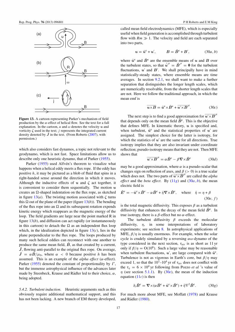
Rep. Prog. Phys. 76 (2013) 096801 P H Roberts and E M King
B
(a)
(b)
BR
u
(c)
B
j
Figure 13. A cartoon representing Parker’s mechanism of fieldproduction by the α-effect of helical flow. See the text for a fullexplanation. In the cartoon, u and ω denotes the velocity u andvorticity ζ used in the text; j represents the integrated currentdensity denoted by J in the text. (From Roberts (2007), withpermission.)
which also considers fast dynamos, a topic not relevant to thegeodynamo, which is not fast. Space limitations allow us todescribe only one heuristic dynamo, that of Parker (1955).
Parker (1955) used Alfven’s theorem to visualize whathappens when a helical eddy meets a flux rope. If the eddy haspositive h, it may be pictured as a blob of fluid that spins in aright-handed sense around the direction in which it moves.Although the inductive effects of u and ζ act together, itis convenient to consider them sequentially. The motion u
creates an -shaped indentation on the flux rope, as sketchedin figure 13(a). The twisting motion associated with ζ turnsthis out of the plane of the paper (figure 13(b)). The bendingof the flux rope into an and its subsequent rotation expendskinetic energy which reappears as the magnetic energy of theloop. The field gradients are large near the point marked R infigure 13(b), and diffusion can act rapidly (or instantaneouslyin this cartoon) to detach the as an independent flux loopwhich, in the idealization depicted in figure 13(c), lies in theplane perpendicular to the flux rope. The loops produced bymany such helical eddies can reconnect with one another toproduce the same mean field, B, as that created by a current,J , flowing anti-parallel to the original flux rope. On average,J = αB/µ0, where α < 0 because positive h has beenassumed. This is an example of the alpha effect (α-effect).Parker (1955) denoted the constant of proportionality by Γ ,but the immense astrophysical influence of the advances latermade by Steenbeck, Krause and Radler led to their choice, α,being adopted.
5.4.2. Turbulent induction. Heuristic arguments such as thisobviously require additional mathematical support, and thishas not been lacking. A new branch of EM theory developed,
called mean field electrodynamics (MFE), which is especiallyuseful when field generation is accomplished through turbulentflow with Rm 1. The velocity and field are each separatedinto two parts,
u = ue + u′, B = Be + B′, (30a, b)
where ue and Be are the ensemble means of u and B overthe turbulent states, so that u′e = B′e = 0 for the turbulentfluctuations, u′ and B′. We shall principally have in mindstatistically-steady states, where ensemble means are timeaverages. In section 9.2.1, we shall want to make a furtherseparation that distinguishes the longer length scales, whichare numerically resolvable, from the shorter length scales thatare not. Here we follow the traditional approach, in which themean emf is
u×B = ue×Be + u′×B′e. (30c)
The next step is to find a good approximation for u′×B′e
that depends only on the mean field Be. This is the objectivethat defines MFE. In kinematic theory, u is specified and,when turbulent, ue and the statistical properties of u′ areassigned. The simplest choice for the latter is isotropy, forwhich the statistics of u′ are the same for all directions. Trueisotropy implies that they are also invariant under coordinatereflection; pseudo-isotropy means that they are not. Then MFEshows that
u′×B′e = αBe − β∇×Be (30d)
may be a good approximation, where α is a pseudo-scalar thatchanges sign on reflection of axes, and β (> 0) is a true scalarwhich does not. The two parts of u′×B′e are called the alphaeffect and the beta effect. By (11g) and (30a, b), the meanelectric field is
Ee = −ue×Be − αBe + η∇×Be, where η = η + β
(30e, f )
is the total magnetic diffusivity. This exposes β as a turbulentdiffusivity that enhances the decay of the mean field Be. Intrue isotropy, there is a β-effect but no α-effect.
The turbulent diffusivity β exceeds the moleculardiffusivity, η, in some interpretations of laboratoryexperiments; see section 8. In astrophysical applications ofMFE, β/η is usually enormous. For example, when the solarcycle is crudely simulated by a reversing αω-dynamo of thetype considered in the next section, τrev is as short as 11 yronly if β/η = O(106). Such a large value may be reasonablewhen turbulent fluctuations, u′, are large compared with ue.Turbulence is not as vigorous in Earth’s core, but β/η mayexceed 1, so that the 103–104 yr of τrev does not conflict withthe τη = 6 × 10⁴ yr following from Pozzo et al ’s value ofη (see section 5.1.1). By (30e), the mean of the inductionequation (11c) is then
∂tBe = ∇×(αBe + ue×Be) + η∇2Be. (30g)
For much more about MFE, see Moffatt (1978) and Krauseand Radler (1980).
17

Rep. Prog. Phys. 76 (2013) 096801 P H Roberts and E M King
5.4.3. Mean field models. When the α term is presentin (30g), Cowling’s theorem does not apply to Be, andself-excited solutions may exist in which Be and ue areaxisymmetric. We denote the axisymmetric parts of ensembleaverages by an overbar without the superfix e. In the torpolrepresentation where B = BT + BS and u = uT + uS (see(16a, d)), axisymmetric poloidal (toroidal) vectors have no(only) φ components:
BT = B(r, θ, t)1φ, BS = ∇×(A(r, θ, t)1φ),
uT = sω(r, θ, t)1φ, uS = ∇×(χ(r, θ, t)1φ).
(31a, b, c, d)
The toroidal parts are trapped in the fluid; BS exists in themantle but uS does not, and χ(ro, θ, t) = χ(ri, θ, t) = 0.These representations transform (30g) into scalar equationsgiven in many publications; see for example section 9.1 ofMoffatt (1978). They are
∂t A + s−1uS · ∇(sA)︸ ︷︷ ︸advection of BS
= αB︸︷︷︸α source of BS
+ η∇21 A︸ ︷︷ ︸
sink of BS
, (32a)
∂t B + suS · ∇(s−1B)︸ ︷︷ ︸advection of BT
= sBS · ∇ω︸ ︷︷ ︸ω source of BT
− (α∇21 A + s−1∇α · ∇(sA))︸ ︷︷ ︸
α source of BT
+ η∇21 B︸ ︷︷ ︸
sink of BT
, (32b)
where ∇21 = ∇2 − s−2. The second terms on the left-hand
sides merely represent advection of field by uS , and are non-regenerative. The solutions of (32a,b) must satisfy boundaryconditions equivalent to the dynamo demands (18g, h).
If the term αB in (32a) is absent, A lacks any source,and the dynamo fails; it is only αB that can defeat Cowling’stheorem. If ω = 0, the alpha source in (32b) is also neededto maintain B. It can do so, only if the alpha effect is largeenough, as measured by the ‘alpha-effect magnetic Reynoldsnumber’, Rmα = αD/η. A mean field dynamo whichoperates solely through the two alpha terms in (32a,b), withoutinvolving ω, is called an α2-dynamo, because it functionsthrough the product of two α terms. The action of ω on BSis the ‘omega effect’ of section 5.2.2, and is quantified by the‘omega-effect magnetic Reynolds number’, Rmω = ωD2/η.If Rmω Rmα , the term involving α in (32b) can beignored, and (32a,b) then define the αω-dynamo. When allterms of (32a,b) are significant, the terminology α2ω-dynamois sometimes used. Very many solutions of each type havebeen published especially in the astrophysical literature. Ithas been found that α2-dynamos tend to be steady, but thatαω-models tend to produce oscillatory fields (though uS maymake them steady). Because Rmω Rmα in an αω-dynamo,Bφ |BS |, but Bφ and |BS | are comparable in an α2-dynamowhere Rmω Rmα . We shall see in section 7 that most MHDdynamo simulations are currently of α2 type.
Parker’s αω-dynamo, like other similar heuristic models,is easy to visualize but is very specific, involving highlylocalized reconnection. Also, the averaging process leading to(30e,g) is hard to make rigorous for realistic turbulent flows.An alternative (Braginsky 1965a, 1965b) is an expansion in
the asymmetry of B and u, i.e. u = u + u′, where u is theaxisymmetric part of u, obtained by averaging its cylindricalcomponents over φ. The first terms of Braginsky’s expansionare (31a–d), with |A/roB| and |χ/r2
o ω| of order Rm−1ω ,
where Rmω 1. (The operative A and χ are so-called‘effective variables’ that depend on, but differ from, thoseappearing in (31b, d).) The additional asymmetric motion,u′, which is O(Rm
−1/2ω u), creates an αω-dynamo in which α
can be explicitly calculated from u and u′. See also Soward(1972) and Soward and Roberts (2014). Braginsky theory ismathematically more rigorous than MFE and may be relevantto the magnetostrophic dynamo considered in section 6.3.2.
6. MHD geodynamo theory
6.1. The cooling Earth model
6.1.1. The adiabat. From here on we shall focus on theother side of core MHD: its fluid dynamics. It was seen insection 1 that both inner and outer cores are made of ironmixed with unknown elements that make them lighter thanpure iron. It will suffice to lump the unknown together, andmodel the core as a binary alloy in which the mass fraction oflight constituents is ξ . The seismically-derived models of theEarth’s interior referenced in section 1 show that, because ofcompression by the weight of overlying material, the density,ρ, of core fluid increases from 9.9×10³ kg m−3 at the CMB to12.2×103 kg m−3 at the ICB. The density of the inner core onits surface is 12.8 × 10³ kg m−3. There is therefore a jump indensity at the ICB of ∆ρ = 600 kg m−3. The mean density ofthe fluid core is ρ = 10.9 × 10³ kg m−3.
The relationship between density ρ and pressure P in thefluid core inferred from seismic data lies close to an adiabat.This strongly suggests that the fluid core is well mixed, so thatξ and the specific entropy, S, are very nearly uniform:
ξ = ξa(t), S = Sa(t). (33a, b)
Here the suffix a stands for ‘adiabatic’, although ‘homentropic’is a more accurate adjective. Time dependence is includedbecause evolution of ξa and Sa on the long geological timescaleis highly significant. Their time derivatives are denoted by ξa
and Sa.Flow speeds, U , in the fluid core are of order 10−8us,
where us is the (P wave) speed of sound. The dynamicpressure gradient, i.e. the pressure gradient associated withthe core flow, u, is therefore negligible compared with thethermodynamic pressure gradient, as is the Lorentz forceas will be apparent later. The force balance in the coreis therefore overwhelmingly a hydrostatic one between thegravitational force and the pressure gradient alone. Thisdefines a motionless reference state deviations from whichare studied below. The reference state is neutrally buoyanteven though its density increases with depth (e.g. Landau andLifshitz (1987), section 4). Thermodynamics and (33a, b)show that the density ρa, pressure Pa and temperature Ta, inthe reference state obey
ρ−1a ∇Pa = ga, ρ−1
a ∇ρa = ga/u2s , T −1
a ∇Ta = γgga/u2s ,
(33c, d, e)
18

Rep. Prog. Phys. 76 (2013) 096801 P H Roberts and E M King
where ga is the gravitational field created by ρa, γg = αTu2s/cP
is Gruneissen’s constant, αT is the thermal expansioncoefficient, and cP is the specific heat at constant P .Seismology determines g and us accurately. Values at theCMB (at the ICB, in parentheses) are g = 10.68(4.40)m s−2
and us = 8.1(10.4) × 103 m s−1. Less reliably known areαT = 1.8(1.0) × 10−5 K−1 and cP = 850(830) J kg−1 K−1,but these values give γg ≈ 1.3–1.4 that is significant in (34).Equation (33e) shows that |∂rTa| increases rapidly with r andis 0.9(0.05) K km−1 at r = ro(r = ri). It also shows thatthe temperature difference, ∆Ta = Ta(ri) − Ta(ro), betweenthe ICB and CMB is about 1300 K; we follow Braginsky andRoberts (1995) by taking Ta = 4000(5300)K.
Because of the finite thermal conductivity, KT, of the core,the adiabatic temperature gradient (33e) pushes heat outward.Because ∂rTa increases rapidly with r , so do the radial adiabaticheat flux, IT
a (r), and the outward adiabatic heat flow, Qa(r),which are
ITa (r) = −KT∂rTa(r), Qa(r) = 4πr2IT
a (r). (33f, g)
The molecular transport properties of materials at the hightemperatures and pressures of the core are notoriouslydifficult to determine. Estimates of KT, typically comefrom either high pressure experiments or so-called ‘firstprinciples’ calculations, the latest of which is 100 W m−1 K−1
(140 W m−1 K−1) at the CMB (ICB) (Pozzo et al 2012),corresponding to a Qa of 13.5 TW (0.7 TW). This estimateaccounts for 30% of the 44 TW heat flow from the Earth’ssurface (Pollack et al 1993). Conduction of heat is associatedwith an entropy flux IS (W m−2 K−1), and an entropy sourceςS (W m−3K−1) that in the reference state are
ISa = 1
TaIT
a = −KT ∇Ta
Ta, ςS
a = KT
(∇Ta
Ta
)2
. (33h, i)
6.1.2. Sources of buoyancy. In geophysical fluids, measureddensity profiles that closely follow adiabatic gradients usuallyindicate convective flow. The motions mixing the core andgenerating the geomagnetic field are generally believed to bedriven by buoyancy. It was at first thought that this was createdthermally by radioactive sources such as 40K dissolved in thecore. Because of radioactive decay, their heat input early inthe Earth’s history would be considerably greater than today.For 40K for example, which has a half-life of 1.25 × 10⁹ yr,the heat input 4.5 × 10⁹ yrs ago would have been 12 timesgreater than today. This might well have repercussions on thestate of the geodynamo possibly great enough to conflict withpaleomagnetic findings. Such considerations and geochemicalarguments (not given here) acted to focus attention on anotherpossibility, which we favor here. For simplicity we entirelyignore radioactivity.
It is now thought that the outer core is buoyant becauseit is cooling through heat loss to the mantle. Cooling a fluidfrom the top promotes convection as surely as heating it fromthe bottom! This secular cooling by global loss of internalenergy is not the only possibility. If the fluid core is cooled
enough, it freezes. An application Lindemann’s law predictsthat solidification occurs at a temperature Ts satisfying
T −1a ∇Ts = 2(γg − 1
3 )g/u2s (34)
(Stacey and Irvine 1977). It was shown above that γg > 13 , so
it follows from (33e) and (34) that the freezing point increasesmore rapidly with increasing pressure than the adiabat. Theresulting phenomenon is unfamiliar in everyday life: when corefluid is cooled sufficiently from the top, it freezes from thebottom!
The prevailing opinion today is that the inner core is theresult of the freezing of the outer core (Jacobs 1953). The ICBis a freezing surface that creeps very slowly upwards as the corecools. The jump ∆ρ in density at the ICB is not only due tocontraction on freezing but also because the solidus is richer iniron than the liquidus (Braginsky 1963). We follow Braginskyand Roberts (1995) by supposing that the part, ∆ξρ, of ∆ρ
due to the jump in composition is 500 kg m−3. The remaining100 kg m−3 is then due to the overall contraction of the Earthas it cools, in which the gravitational energy released does nothelp to drive the geodynamo, unlike ∆ξρ which does. Thefreezing of the inner core therefore provides not only thermalbuoyancy from the release of latent heat at the ICB, but alsocompositional buoyancy, as the light alloying core constituentξ is released during freezing. In short, the slowly growing ICBfosters thermochemical convection.
In this cooling Earth model of geomagnetism, the twobuoyancy sources are proportional to one another and tothe rate of inner core solidification ri . If the rate, Mi , atwhich the mass Mi of the inner core increases is constantand that it has been forming over the entire age of the Earth,τage ≈ 4.5 × 10⁹ yr, then ri = ri/3τage ≈ 2.9 × 10⁻¹² m s−1,and Mi ≈ 6.8 × 10⁵ kg s−1, which releases latent heat atthe rate hMi ≈ 0.7 TW, assuming a latent heat of h =106 J kg−1. This is only very approximate because h isuncertain. The rate of release of gravitational energy canbe more accurately estimated from ri : 0.25 TW according toLoper (1984); 0.28 TW according to Braginsky and Roberts(1995, appendix B). It seems certain that the thermal andcompositional sources together are sufficient to power thegeodynamo. Braginsky and Roberts (1995) and Labrosse(2003) raise the possibility that the inner core may have startedto form much more recently. If τage is redefined to be the ageof the inner core, and the estimate τage = 109 yr of Labrosse(2003) accepted, ri and the energy sources are increased bya factor of 4.5. Prior to the birth of the inner core, and inthe presumed absence of radiogenic heating, core convectionwould have to be powered only by the escape of internal energy.For more detailed discussion of the tight energy budget in thecore, see Braginsky and Roberts (1995).
The cooling Earth model is utterly dependent on heatescaping from the core into the mantle, and therefore onthe efficacy of mantle convection. Any vagaries in mantleconvection affecting the heat it takes from the core cansignificantly affect convection in the core and the geodynamo.The mantle acts as a valve that, if closed, would quicklytransform the adiabatic core into an isothermal fluid mass that,being negatively buoyant, would soon become stagnant. It
19
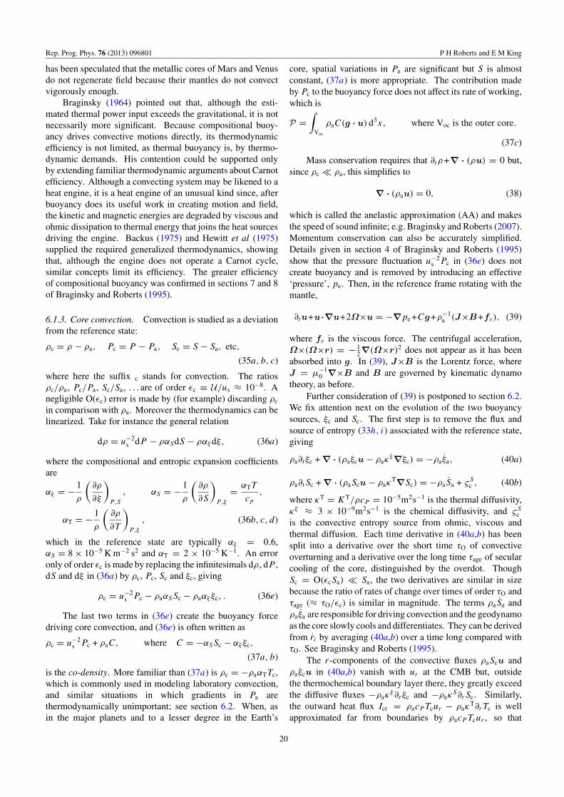
Rep. Prog. Phys. 76 (2013) 096801 P H Roberts and E M King
has been speculated that the metallic cores of Mars and Venusdo not regenerate field because their mantles do not convectvigorously enough.
Braginsky (1964) pointed out that, although the esti-mated thermal power input exceeds the gravitational, it is notnecessarily more significant. Because compositional buoy-ancy drives convective motions directly, its thermodynamicefficiency is not limited, as thermal buoyancy is, by thermo-dynamic demands. His contention could be supported onlyby extending familiar thermodynamic arguments about Carnotefficiency. Although a convecting system may be likened to aheat engine, it is a heat engine of an unusual kind since, afterbuoyancy does its useful work in creating motion and field,the kinetic and magnetic energies are degraded by viscous andohmic dissipation to thermal energy that joins the heat sourcesdriving the engine. Backus (1975) and Hewitt et al (1975)supplied the required generalized thermodynamics, showingthat, although the engine does not operate a Carnot cycle,similar concepts limit its efficiency. The greater efficiencyof compositional buoyancy was confirmed in sections 7 and 8of Braginsky and Roberts (1995).
6.1.3. Core convection. Convection is studied as a deviationfrom the reference state:
ρc = ρ − ρa, Pc = P − Pa, Sc = S − Sa, etc,
(35a, b, c)
where here the suffix c stands for convection. The ratiosρc/ρa, Pc/Pa, Sc/Sa, . . . are of order εc ≡ U/us ≈ 10−8. Anegligible O(εc) error is made by (for example) discarding ρc
in comparison with ρa. Moreover the thermodynamics can belinearized. Take for instance the general relation
dρ = u−2s dP − ραSdS − ραξdξ, (36a)
where the compositional and entropic expansion coefficientsare
αξ = − 1
ρ
(∂ρ
∂ξ
)P,S
, αS = − 1
ρ
(∂ρ
∂S
)P,ξ
= αTT
cp,
αT = − 1
ρ
(∂ρ
∂T
)P,ξ
, (36b, c, d)
which in the reference state are typically αξ = 0.6,αS = 8 × 10⁻⁵ K m−2 s2 and αT = 2 × 10⁻⁵ K−1. An erroronly of order εc is made by replacing the infinitesimals dρ, dP ,dS and dξ in (36a) by ρc, Pc, Sc and ξc, giving
ρc = u−2s Pc − ρaαSSc − ρaαξξc, . (36e)
The last two terms in (36e) create the buoyancy forcedriving core convection, and (36e) is often written as
ρc = u−2s Pc + ρaC, where C = −αSSc − αξξc,
(37a, b)
is the co-density. More familiar than (37a) is ρc = −ρaαTTc,which is commonly used in modeling laboratory convection,and similar situations in which gradients in Pa arethermodynamically unimportant; see section 6.2. When, asin the major planets and to a lesser degree in the Earth’s
core, spatial variations in Pa are significant but S is almostconstant, (37a) is more appropriate. The contribution madeby Pc to the buoyancy force does not affect its rate of working,which is
P =∫
Voc
ρaC(g · u) d3x, where Voc is the outer core.
(37c)
Mass conservation requires that ∂tρ+∇ · (ρu) = 0 but,since ρc ρa, this simplifies to
∇ · (ρau) = 0, (38)
which is called the anelastic approximation (AA) and makesthe speed of sound infinite; e.g. Braginsky and Roberts (2007).Momentum conservation can also be accurately simplified.Details given in section 4 of Braginsky and Roberts (1995)show that the pressure fluctuation u−2
s Pc in (36e) does notcreate buoyancy and is removed by introducing an effective‘pressure’, pe. Then, in the reference frame rotating with themantle,
∂tu+u·∇u+2Ω×u = −∇pe +Cg+ρ−1a (J×B+fν), (39)
where fν is the viscous force. The centrifugal acceleration,Ω×(Ω×r) = − 1
2∇(Ω×r)2 does not appear as it has beenabsorbed into g. In (39), J×B is the Lorentz force, whereJ = µ−1
0 ∇×B and B are governed by kinematic dynamotheory, as before.
Further consideration of (39) is postponed to section 6.2.We fix attention next on the evolution of the two buoyancysources, ξc and Sc. The first step is to remove the flux andsource of entropy (33h, i) associated with the reference state,giving
ρa∂t ξc + ∇ · (ρaξcu − ρaκξ∇ξc) = −ρa ξa, (40a)
ρa∂tSc + ∇ · (ρaScu − ρaκT∇Sc) = −ρaSa + ςS
c , (40b)
where κT = KT/ρcP = 10−5m2s−1 is the thermal diffusivity,κξ ≈ 3 × 10⁻⁹m2s−1 is the chemical diffusivity, and ςS
cis the convective entropy source from ohmic, viscous andthermal diffusion. Each time derivative in (40a,b) has beensplit into a derivative over the short time τO of convectiveoverturning and a derivative over the long time τage of secularcooling of the core, distinguished by the overdot. ThoughSc = O(εcSa) Sa, the two derivatives are similar in sizebecause the ratio of rates of change over times of order τO andτage (≈ τO/εc) is similar in magnitude. The terms ρaSa andρa ξa are responsible for driving convection and the geodynamoas the core slowly cools and differentiates. They can be derivedfrom ri by averaging (40a,b) over a time long compared withτO. See Braginsky and Roberts (1995).
The r-components of the convective fluxes ρaScu andρaξcu in (40a,b) vanish with ur at the CMB but, outsidethe thermochemical boundary layer there, they greatly exceedthe diffusive fluxes −ρaκ
ξ∂rξc and −ρaκS∂rSc. Similarly,
the outward heat flux Icr = ρacP Tcur − ρaκT∂rTc is well
approximated far from boundaries by ρacP Tcur , so that
20

Rep. Prog. Phys. 76 (2013) 096801 P H Roberts and E M King
the outward convective heat flow through the geocenteredspherical surface S(r) is
Qc(r) = ρacP 〈Tcur〉A, (40c)
where A = 4πr2 is the area of S(r) and the angle brackets, asin (8b), denote the average over S(r) of the quantity betweenthem. The average 〈Tcur〉 is positive because the temperature,T +
c (T −c ) of hot (cold) fluid is rising (sinking) at a speed
|ur | = O(U), so that T ±c ur > 0 for both and 〈Tcur〉 ≈ U∆Tc,
where ∆Tc = T +c − T −
c is the difference in the temperaturesof the rising and falling streams. On approaching the CMBand crossing the edge r = r−
o of the boundary layer there, ∂rTc
grows and the diffusive flux −ρaκT∂rTc takes over from the
diminishing convective flux ρacP 〈Tcur〉, so that Icr remains thesame. We may adopt Icr = ρacP 〈Tcur〉 at the CMB providedwe recognize that ur is to be interpreted as the radial velocityat the inner edge, r = r−
o , of the boundary layer there. Withthis understanding, the convective heat flow to the mantle is
Qc(ro) = ρacP 〈Tcur〉ro Ao ≈ ρacP AoU∆Tc, (40d)
where Ao = A(ro) = 1.522 × 10¹⁴ m2.The total outward heat flow is Q(r) = Qa(r) + Qc(r),
where Qa is the adiabatic heat flow (33g). Estimates of theheat flow, Q(ro), to the mantle range between 3 and 20 TW, butit cannot be greater than the heat flow from the Earth’s surface,of about 44 TW (Pollack et al 1993). Taking Q(ro) < 44 TWin (40d), we obtain ∆Tc < 4×10⁻⁴ K, which is tiny comparedwith ∆T = Ta(ri) − Ta(ro) ≈ 1300 K. This gives a posteriorisupport for the claim that the temperature of the core is closelyadiabatic. Below we shall make estimates using∆Tc = 10−5 Kbut it is clear that this value is rather uncertain.
The uncertainty in the heat flow from the core invites thequestion of what happens if the total heat flow to the mantle,Q(ro)(= Qa(ro) + Qc(ro)), though positive, is less than theadiabatic heat flow Qa(ro). In this case, a stable layer formsat the top of the core in which ∂rS > 0, Qc(r) < Qa(r)
and Qc(r) < 0, so that convection carries heat downwards(Loper 1978). This layer is thin if compositional buoyancyoverwhelms thermal buoyancy sufficiently to maintain thewell-mixed adiabatic state except in the layer. A commonlyused dimensionless measure of the heat flow from a convectingsystem is the ratio of the total heat flow to the conductive heatflow. This is called the Nusselt number, Nu, and usually mustexceed 1 if the system is convecting. For the core Nu =Q(ro)/Qa(ro) and is less than 1 if Qc(ro) < 0 even though thesystem is still convecting somewhere below the CMB.
The cooling Earth model outlined in this section dominatesgeodynamo theory today, but two other power sourcesmay have been underestimated. First, although dissolvedradioactivity was ignored above, it may be an importantsource, particularly in the early Earth. The second potentiallyimportant power source is owed to the mechanical coupling ofthe core and mantle.
6.1.4. Core-mantle coupling. Core and mantle are coupledtogether both thermally and mechanically. Mechanicalcoupling is accomplished by viscous, magnetic, gravitational
and topographic torques acting across the CMB, and is a topicrecently reviewed by Roberts and Aurnou (2012). Mechanicalcoupling allows for the possibility that core motions arederived from the abundant rotational energy of the mantle.Specifically, it has been argued that energy extracted fromthe luni-solar precession is potentially sufficient to maintainthe geomagnetic field over all geological time (Bullard 1949,Kerswell 1996). Work continues exploring that possibility(see section 8.1.4).
The mechanical link between core dynamics and therotation of the mantle may also provide an alternative means toprobe core physics using surface observations, supplementingthe geomagnetic observations discussed in part 1. For example,as we discuss in section 6.3.3, torsional waves travelingthrough the core produce EM torques that can affect therotation rate of the mantle (length of day). Another importantobservation for the present review is the work of Buffett (2010),which infers the field strength within the core by consideringhow the direction of Earth’s rotation axis is changing.
Misalignment between Earth’s equatorial plane and theorbital planes of the Earth–Sun and Earth–Moon systemsproduce torques on Earth’s tidal bulge that result in aweak ‘wobbling’ of Earth’s rotation, called nutations.Measurements of nutations reveal temporal phase lags betweentidal forcing and Earth’s response that are attributed todissipation within the planet. Buffett (2010) uses estimatesof ohmic dissipation due to tidally forced flow in thecore to account for previously unexplained phase lags, andthese estimates require B ≈ 3 mT to produce the requireddissipation. This internal core field strength estimate is anorder of magnitude stronger than the radial CMB field (seefigure 5), but is consistent with theoretical arguments forinternal core field strength given in sections 5.4.3, 6.3.2, 6.4.3and 7.6.2. We adopt this value of B here.
For the remainder of this section only thermal couplingis considered. According to the preceding description ofthe cooling Earth model, heat escapes from the core intothe overlying mantle. The mantle, which is also heated byradioactive elements, cools to space on its surface and issuperdiabatic. It convects, despite its very high viscosity andthis convection is expressed as tectonic motions on Earth’ssurface.
The appropriate dimensionless measure of the importanceof buoyancy forces in mantle dynamics is the traditionalRayleigh number, R, where ‘traditional’ has to be includedso that R can be distinguished from the Rayleigh number Ra
used below for core convection. Here
R = goa3αT∆T/ν κ, (41)
where g is gravitational acceleration, αT is thermal expansivity,∆T is the difference in the temperatures of the CMB andEarth’s surface, ν is the kinematic viscosity and κ is the thermaldiffusivity. Convection can occur only if R exceeds a criticalvalue Rc = O(103). The existence of convective motions in themantle shows that the mantle is in the supercritical convectivestate R > Rc. Seismically derived temperature profiles for themantle give estimates of R = O(106). The typical convectivevelocity of the mantle can be estimated by observed tectonic
21

Rep. Prog. Phys. 76 (2013) 096801 P H Roberts and E M King
motions, U = O(10−9)m s−1. These distinct observationalconstraints are consistent with classical boundary layer theoryfor convection (Turcotte and Oxburgh 1967).
The overturning time for the mantle, analogous to τO
defined for the core in section 3.1, is τO = ro/U ≈ 200 Myr,comparable with the geologic time scale, τage. It is natural tosuppose that the style of mantle convection varies over geologictime on the τO time scale, resulting in an ever changing corecooling rate and a different geodynamo. This might explainwhy the Cretaceous and Permo-Carboniferous superchronshappened (see figure 10) and why their 35 and 50 Myr durationsare far longer than any natural time scale of the core: the mantleis responsible.
Further progress depends on a better understanding ofthe coupled core–mantle system, but the enormously differenttimescales for mantle and core convection presents theory witha difficulty: it is impractical to treat core and mantle as a singlesystem, in which the temperature T and outward heat fluxITr are continuous at the CMB. It is however impossible to
use both these conditions when solving for mantle and coreindividually, as that would over-determine the solutions. Afull thermodynamic treatment reveals that the optimum wayof treating core and mantle as separate systems is to solvefor the mantle using specified T at the CMB, and to solvefor the core using specified IT
r on the CMB (e.g. Braginskyand Roberts (2007)). The latter is determined by solving themantle equations and the former by solving the core equationsunder these specified boundary conditions. (Most simulationsof core MHD ignore this by specifying T on the CMB, as weshall do in the next section; see (44c, d).)
Having resolved the question of how to study mantleand core dynamics separately, we direct attention to mantleconvection. This is an immense geophysical topic that isbeyond the competence of the present authors. Fortunatelyit is one that need not be studied in depth here. For a moredetailed account of the subject, see Schubert et al (2001). Thefollowing makes only a few relevant observations.
The style of mantle convection is very different from thatof core convection because the viscosity ν of the mantle is verygreat: ν ≈ 1019 m2 s−1. The Reynolds number is thereforetiny: Re = Ua/ν ≈ 10−21, well below the threshold for normalturbulence. Inertia has no role in mantle convection. Thethermal diffusivity, κ , is however comparable with κT in thecore (see (40b)). If κ = 10−6 m2 s−1, the Peclet number, P e =Ua/κ , is of order 104, indicating that convective heat transportis more important than conductive, and that the mantle is ina state that is sometimes called ‘thermal turbulence’. In thisstate, IT
r (ro, θ, φ) may be expected to vary only on the τO timescale, so that it can be assumed time independent in studyingcore dynamics. It will however depend on θ and φ, i.e. notbe uniform over the CMB. Spatially heterogeneous thermalboundary conditions at the CMB are usually ignored in studiesof core convection, and will be for the remainder of this section,but see section 7.4.
6.2. A simplified cooling Earth model
Section 8 of Braginsky and Roberts (1995), develops a‘homogeneous model’ of the last section, in which Sa and ξa
are spatially uniform (∇Sa = ∇ξa = 0) but in whichcore convection is still driven by core cooling (Sa < 0,ξa > 0). This model is quite close to the one that nearly allgeodynamo simulators currently prefer to use, which employsthe Boussinesq approximation (BA). This ignores the secularevolution of the core, the consequences of freezing at the ICBbeing replaced by equivalent sources of composition and heatthat are independent of t . We call this ‘the simplified coolingEarth model’ even though no cooling takes place!
The BA assumes that core fluid is incompressible;therefore in the basic well-mixed reference state,
ξ = ξa = constant, T = Ta = constant, (42a, b)
instead of (33a, b); ρ = ρ0 = constant too. Incompressibilityalso implies that, as for the basic state (33a, b) of section 6.1,the reference state (42a, b) is neutrally buoyant. As before,deviations from this state are denoted by c. For ρc, (36a, b)are replaced by
ρc = ρ0Cc, where Cc = −αξξc − αTTc. (42c, d)
The BA is commonly used in describing convectionexperiments in the laboratory. When applied to the core,incompressibility introduces errors of order (ρi − ρo)/ρ ≈20%. These are smaller than other geophysical uncertainties,such as those created by the unknown chemical compositionof the core, by the poorly known values of relevantphysical parameters, and by the crude treatment of turbulence(section 9.2). While reliance on the BA entails loss of(geo)physical realism, it simplifies the treatment of geostrophyin section 6.3 and further developments below. Only fordynamos in the gaseous planets, the Sun and stars, does theBA introduce substantial errors.
We simplify our treatment of the Boussinesq geodynamofurther by ignoring compositional buoyancy, so thatρc = −ρ0αTTc. Because ρ0 is constant, (38) becomes
∇ · u = 0. (43a)
The equation of motion (39) simplifies to
∂tu + u · ∇u︸ ︷︷ ︸Inertia
+ 2Ω×u︸ ︷︷ ︸Coriolis
= − ∇pe︸︷︷︸pressure
+ γ0αTTcr︸ ︷︷ ︸buoyancy
+ ρ−1a J×B︸ ︷︷ ︸Lorentz
+ ν∇2u︸ ︷︷ ︸viscosity
, (43b)
where pe = Pc/ρa is the effective ‘pressure’; Tc obeys the heatconduction equation
∂tTc + u · ∇Tc = κ∇2Tc + H, (43c)
where κ here and below replaces κT because κξ is no longerinvolved. The kinematic dynamo theory of section 5.1 stillapplies so that
∂tB = ∇×(u×B) + η∇2B, ∇ · B = 0. (43d, e)
The accelerations are named in (43b), which is the relevantform of the Navier–Stokes equation in this article. Thegradient of pe has no thermodynamic significance in the BA,its purpose now being merely to ensure that solutions of (43b)
22

Rep. Prog. Phys. 76 (2013) 096801 P H Roberts and E M King
Table 1. Basic physical properties of the core.
Dimensionless NumbersSymbol Name of number Definition core
Ra Rayleigh goDαT∆Tc/2Ωκ 109
Λ Elsasser B2/2Ωηµ0ρ0 10Ro Rossby U/2ΩD 10−6
E Ekman ν/2ΩD2 10−15
Rm Magnetic Reynolds UD/η = RoPm/E 1300Pm Magnetic Prandtl ν/η 1.7 × 10⁻⁶
Pr Prandtl ν/κ 0.1q Diffusivity ratio κ/η 1.7 × 10⁻⁵
Ha Hartmann BD/(νηµ0ρ0)1/2 = VAD/(νη)1/2 7 × 10⁷
Rom Magnetic Rossby B/2ΩD(µ0ρ0)1/2 = VA/2ΩD 8 × 10⁻⁵
Pe Peclet UD/κ = RoPr/E 9 × 10⁷
Re Reynolds UD/ν=Ro/E 9 × 10⁸
Symbol Name Value Unit
D Depth of fluid core = ro − ri 2.255 × 10⁶ mU Typical fluid velocity 4 × 10⁻⁴ m s−1
Ω Angular velocity of Earth 7.29 × 10⁻⁵ s−1
η Magnetic diffusivity = 1/µ0σ 0.7 m2 s−1
ν Kinematic viscosity 10−6 m2 s−1
κ Thermal diffusivity 10−5 m2 s−1
go Gravitational acceleration at CMB 10.68 m s−2
γ0 go/ro 3.07 × 10⁻⁶ s−2
αT Coefficient of thermal expansion 10−5 K−1
∆T Temperature contrast = Ti − To 1300 K∆Tc Superadiabatic temperature contrast 10−5 KB Typical magnetic field strength 3 × 10−3 TB
gs Rms of s-component of B 10−3 T
µ0 Magnetic permeability 4π × 10−7 H m−1
ρ0 Core density 1.1 × 10⁴ kg m−3
VA Alfven velocity=B/(µ0ρ0)1/2 3 × 10⁻² m s−1
VgA Torsional wave velocity=Bg
s /(µ0ρ0)1/2 10−2 m s−1
satisfy (43a). In the buoyancy force, Tc is often calledthe ‘superadiabatic temperature’, though strictly adiabatsare meaningless in the BA. The gravitational acceleration,g = −γ0r, is assumed proportional to r with γ0 = 3.07 ×10⁻⁶ s−2, which gives go (= |g(ro)|) correctly (although itimplies gi (= |g(ri)|) = 3.75 m s−2 instead of 4.40 m s−2,again a 20% error). Because of (43a), the viscous forcefν in (43b) simplifies for constant ν to ρ0ν∇2u. In (43c),H = T0ς
Sc /ρ0cp, where ςS
c is the entropy source appearingin (40b). We shall assume for simplicity that H = 0.
Solutions of (43a–e) must satisfy appropriate boundarydemands, important amongst which are the dynamoconditions (18g, h) on the CMB. Usually u is required tosatisfy no-slip conditions on CMB and ICB:
u(ro) = 0, u(ri) = Ωi×r, (44a, b)
where Ωi is the angular velocity of the solid inner core, whichis supposed to have the same electrical conductivity as thefluid core, so that B and r×E are continuous on the ICB. Thechoice of the mantle as reference frame imposes (44a), andΩi is determined by the viscous and magnetic torques actingacross the ICB; and it is reasonable to take Ωi = Ωi1z becauseof gyroscopic torques. The solution of (43c) is required tosatisfy
Tc(ro) = To = constant, Tc(ri) = Ti = constant, (44c, d)
and ∆Tc = Ti − To = constant. In section 6.3.2, we shallconsider inviscid dynamo models, for which ν∇2u is omittedfrom (43b), and (44a, b) are replaced by
ur(ro) = 0, ur(ri) = 0. (44e, f )
The BA specification of the MHD dynamo problem is nowcomplete. If (u, B, Tc) is a solution of (43) satisfying (44), sois (u, −B, Tc). This fact is what makes the dynamo the onlyplausible explanation of the Earth’s magnetism (section 4).The vigor of convection in the BA model depends, not on therate of cooling of the core, but on ∆Tc, which we quantify bythe Rayleigh number, Ra. This is defined in table 1, where itis joined by other relevant dimensionless numbers. Beneaththe table is a list of the physical quantities used in definingthe parameters and their estimated values for the core. TheRayleigh number is the most important input parameter ofthe theory, a prime objective of which is the evaluation ofthe output parameters, Ro and Λ. These are dimensionlessmeasures of the flow speed U and field strength B and are alsolisted in table 1. They are called the Rossby number and theElsasser number, named in honor of Elsasser (1946), who firstsuggested that the Lorentz force might equilibrate with theCoriolis force in the core.
The predictability of the governing equations (43a–e) canbe estimated as for meteorological forecasts. To do so, a small
23
Rep. Prog. Phys. 76 (2013) 096801 P H Roberts and E M King
error is introduced into the integration and the average time ittakes to double is evaluated. Hulot et al (2010) find that this‘doubling time’ is just a few decades for the geodynamo. Thus,solutions of (43a–e) are chaotic, and the so-called ‘butterflyeffect’ limits forecasting to less than even one overturning time,τO. This forecasting horizon illustrates the strongly nonlinearnature of the geodynamo problem.
A useful consequence of (43a,b) is the vorticity equation
∂tζ + u · ∇ζ − (2Ω + ζ) · ∇u
= γ0αT∇Tc×r + ρ−10 ∇×(J×B) + ν∇2ζ, (45)
where ζ (= ∇×u) is the vorticity in the mantle frame and2Ω + ζ is the vorticity in the inertial frame.
For u = 0, (43c) has a conduction solutionsatisfying (44c, d):
T0(r) = ri
D
( ro
r− 1
)Ti +
ro
D
(1 − ri
r
)To,
for whichdT0
dr= − rori∆T
D r2, (46a, b)
so that the heat flow out of S(r) is Q0 = 4πroriKT∆T/D.
The existence of the conduction solution was noted andignored in writing (40c). This was because section 6.1 wasconcerned only with strong convection, where the heat flowQc given by (40c) greatly exceeds Q0. For the more moderateconvection considered below, we must recognize that Tc andQc are partially created by conduction. From now onwards,the suffix c denotes a deviation from the reference state createdby both convection and conduction. These may be separatedby writing
Tc(r, t) = T0(r) + (r, t), pe(r, t) = p0(r) + Π(r, t),
Qc(r) = Q0 + Q(r), (46c, d, e)
where drp0 = γ0rαTT0. Equations (43b, c) become
∂tu + u · ∇u + 2Ω×u
= −∇Π + γ0αTr + ρ−10 J×B + ν∇2u, (46f )
∂t + u · ∇ + urdrT0 = κ∇2. (46g)
The vorticity equation following from (46f ) is again (45) withTc replaced by .
From the magnitude of the convective heat loss,QCMB (= Q(ro)) to the mantle, estimated in section 6.1.3, thecharacteristic Tc(r, t) away from boundaries is very small, andTc, according to the discussion following (40d), is of theorder of 10−5 K, while is then of order T by (46b, c), i.e.much larger. For the more moderate convection consideredbelow, Tc and may be comparable in size. Then theconduction flux, Q0, must be added into the denominator ofthe definition Nu = Q(ro)/Qa(ro) of the Nusselt number insection 6.1.3. As Qa(ro) = 0 in the BA, the re-defined Nusseltnumber is
Nu = Q(ro)/Q0. (46h)
Now Nu = 1 separates the convecting and non-convectingstates, and Nu − 1 is small when convection is weak. ForNu 1, |∇Tc| |drT0| except near boundaries.
6.2.1. Power integrals. The BA equations (43) and (44)imply two power integrals, one already given in (14c, d);the other is the volume integral of the scalar product of ρ0u
with (43b),
∂tK = P − F − Qν, where K =∫
Vo
1
2ρ0u
2d3x
(47a, b)
is the kinetic energy, P is the buoyant power input (see (37c)for general sources of buoyancy) and Qν is the rate of viscousheating,
P =∫
Voc
ρ0γ0αTTc(r · u) d3x, Qν =∫
Voc
ρ0νζ2d3x,
(47c, d)
these integrals being over Voc, the outer core. The flow losesenergy K at the rate F and the magnetic energy M acquiresit at the same rate; see (14f ). Thus the two F cancel when(47a) and (11d) are summed:
∂t (K + M) = P − Qνη where Qνη = Qν + Qη
(47e, f )
is the total dissipation. Equation (47e) is the energy budgetof the convective dynamo. The power balance for a steadilyoperating dynamo (defined in section 5.1.2) is
Pτ = Qτνη = Qτ
ν + Qτη. (47g)
The estimates U = 4 × 10⁻⁴m s−1 and B = 3 mT giveKτ /Mτ ≈ µ0ρ0U2/B2 ≈ 2 × 10⁻⁴, which is far fromequipartition of energy, the magnetic energy being dominant;see figure 6. (In the inertial frame, the opposite is true.)
An important property of a liquid metal, such as core fluid,is its magnetic Prandtl number, Pm:
Pm ≡ ν/η = 1.7 × 10⁻⁶. (48a)
See table 1. The smallness of Pm in the core suggests thatviscous dissipation is small compared with ohmic, i.e. that
fν = Qτν/Pτ is much smaller than fη = Qτ
η/Pτ . (48b, c)
By (24) and (47d), the ratio of dissipations, fν/η = Qτν/Qτ
η
can be estimated as
fν/η ≈ µ0ρ0νU2L2B/ηB2L2
U = Pm(LB/LU )2Kτ /Mτ ,
(48d)
where LB and LU are the characteristic length scales of fieldand flow; ∇ × B ≈ B/LB and ∇ × u ≈ U/LU . These areimportant length scales, which may be orders of magnitudeapart, and may offset the effect of small Pm to some extent. Itwas argued in section 5.2.2 that the characteristic length scaleof field LB = Rm−1/2D ≈ 60 km. The characteristic scaleof flow, LU , is more difficult to estimate, but a sensible lowerbound is LU E1/3D ≈ 30 m, where E is the Ekman number;see section 7.6. These estimates give
fν/η < PmRm−1E−2/3(Kτ /Mτ ) ≈ 10−3. (48e)
24
Rep. Prog. Phys. 76 (2013) 096801 P H Roberts and E M King
In the magnetostrophic dynamo discussed in section 6.3.2, weexpect LU ∼ LB , and so fν/η would be much smaller still.These estimates suggest that in a steadily operating dynamo
Qτν Qτ
η and Pτ ≈ Qτη, (48f, g)
by (47g). Armed with this revelation, we can use (24)to estimate the power requirement for the geodynamo:Pτ ≈ 0.2 TW.
6.3. Rotational dominance; Proudman–Taylor theorem;CMHD
Some of the complications of geodynamo theory arisefrom the competition between the different forces operatingin (43b). The following discussion attempts simplification byconsidering the action of some forces in the absence of others.
Only one force gives core MHD a preferred direction, theCoriolis force, which is defined by Oz, the direction of Ω. Itis not surprising that core flow u responds by having Oz asits preferred direction, a preference then shared by B and theLorentz force J×B because they are produced by u. This iswhy the compass needle is north seeking. That it does not pointprecisely north may be the way core MHD evades Cowling’stheorem. What is surprising is how important Coriolis forcesare, as assessed by the smallness of Ro and the Ekman number,E; according to table 1, E = 10−15 and Ro = 10−6. One mustconclude that, at least for the largest scalesD, the viscous forceand inertial force are dominated by the Coriolis force. Theresulting MHD is so different from classical MHD that it issometimes called Coriolis magnetohydrodynamics (CMHD).From the extreme smallness of E, the viscous force will be thelast to be included in the following developments.
6.3.1. Geostrophy. If only the Coriolis force and pressuregradient are retained in the momentum equation, there is ageostrophic force balance,
2Ω×u = −∇pe, ∇ · u = 0. (49a, b)
Curling away the pressure gives
∂zu = 0, i.e. u = u(x, y, t). (49c, d)
This is the famous
Proudman–Taylor (PT) theorem:
The slow motion ofan inviscid rotatingfluid is two-dimensional.
Proudman (1916), Taylor (1916). For an axisymmetricboundary such as the CMB, the flow must by (44e, f ) bezonal:
u = u(s, t)1φ. (49e)
This type of motion is called geostrophic flow, and is depictedin figure 14. As (49e) implies ur ≡ 0, geostrophic motions donot convect heat out of the core. Each geostrophic cylinder,C(s), of radius s rotates independently about Oz as a solid body.
Figure 14. A schematic depiction of geostrophic cylinders (C(s)) inthe outer core. The ICB is shown as the central sphere, and theCMB as the surrounding shell. The tangent cylinder is labeled ‘TC’.
Each cylinder has two polar caps on So, denoted by N (s) andS(s) and respectively defined by 0 θ sin−1(s/ro) andπ θ π − sin−1(s/ro). Together they form a closedsurface surrounding a volume which we denote by I(s). Thecylinder C(ri), touching the solid inner core on its equator iscalled the tangent cylinder (TC). The dynamics of the fluid corewithin C(ri) differs from the dynamics outside it. To simplifythe analysis in what follows, we shall often, as in section 5,ignore the inner core, so that D = ro.
The more general flows described later in this section, havegeostrophic and non-geostrophic parts, and the determinationof the latter is sometimes a central issue. They may beseparated by introducing the geostrophic average of a flowthrough its φ-component:
¯ugφ(s) = 1
A(s)
∫C(s)
uφ(x)d2x, (50a)
where A(s) = 4πsz1(s) is the area of C(s) andz1 = √
(r2o − s2). It carries a double bar as it is an average
over both φ and z. The non-geostrophic ung is defined from uby removing its geostrophic part, so that
u(s, φ, z) = ung(s, φ, z) + ¯ugφ(s)1φ. (50b)
As an illustration, consider the thermal wind, which ariseswhen buoyancy is restored to (43a,b):
2Ω×u = −∇pe + γ0αTTcr , ∇ · u = 0. (51a, b)
These have axisymmetric solutions, where Tc = Tc(r, θ) andu = uφ(s, z)1φ is zonal:
uφ = γ0αT
2
∫ z
0∂θ Tc dz + u0(s), (51c)
where u0(s) is arbitrary. On substituting uφ into (50a) andintegrating, the non-geostrophic part, u
ngφ , of uφ is uniquely
determined as uφ − ¯ugφ . It is independent of the choice of 0
as the lower limit of the integral in (51c) and depends only onthe gradient of the assumed Tc. All the arbitrariness in uφ is
25
Rep. Prog. Phys. 76 (2013) 096801 P H Roberts and E M King
confined to its geostrophic part ¯ugφ(s)1φ , which depends on u0
and the integral’s lower limit.The thermal wind exists when there are temperatures
differences between poles and equator. The ω-effect of ung
is usually significant, but the geostrophic shear ¯ugφ is not an
effective generator, as Childress showed; see p 192 of Roberts(1971). When magnetic field is included there is also a zonalmagnetic wind, but that too is not an effective generator; seee.g. section 5.4 of Roberts and Gubbins (1987).
6.3.2. Magnetostrophy; Taylor’s constraint and prescription.The smallness of E and Ro suggests that the Lorentz force isthe next force that should be restored to (43b). The equationsgoverning magnetostrophic flow (MS flow) follow:
2Ω×u = −∇pe + γ0αTTcr + ρ−10 J×B, ∇ · u = 0,
(52a, b)
where µ0J = ∇×B. Equation (52a) expresses aMAC balance between Magnetic, Archimedean and Coriolisforces, where ‘Archimedean’ replaces ‘buoyancy’ to makethe acronym MAC pronounceable. As (52a), like the earlier(49a, b) and (51a), lacks a time derivative, it is often calleda diagnostic equation, to distinguish it from a predictiveequation, like its parent (43b). It will be seen below thatsolving diagnostic equations raises a fresh issue: dynamicconsistency.
On assessing the magnitude of J from Ohm’s law asσUB and the magnitude of J×B as σUB2, it is seen from(52a) that the Elsasser number, Λ, given in table 1 measuresthe relative strengths of the Lorentz and Coriolis forces. Itis independent of velocity and length scales. Alternatively,recalling the representation (22a, b) of the Lorentz force, theratio of the last and first terms in (52a) is the dynamic Elsassernumber (Soderlund et al 2012), Λd = (B2/µ0ρ0LB)
/(2ΩU),
which will arise in section 7.6.2. As viscosity does not appearin (52a), nor do the Prandtl numbers Pr and Pm; only thediffusivity ratio, q = κ/η, is significant (see table 1). Becauseν = 0, the boundary conditions (44a, b) over-determine u
and are replaced by (44e, f ), but for simplicity we continue toignore the inner core, so that only (44e) is relevant:
ur(ro, θ, φ) = 0. (52c)
Solutions of the MS equations evolve on the MAC ormagnetostrophic time scale (Braginsky 1967):
τMS = 2Ωr2o/V
2A, where VA = B/
√(µ0ρ0) (53a, b)
is the Alfven velocity. For B = 3 mT, VA = 3 cm s−1
and τMS = 40 000 yr. Interestingly, the MS time scale andthe magnetic diffusive time essentially coincide when theElsasser number is π2. Because the magnetic Rossby number,Rom = VA/2Ωro ≈ 3 × 10⁻⁵ is so small, Alfven waves andtheir time scale τA = ro/VA = RomτMS are very much lesssignificant in CMHD than in non-rotating MHD. They play norole whatever in MS systems because inertia is completelyabsent from (52a), and the generic VA is no more than aconvenient abbreviation. The time scale τA of non-rotatingMHD is replaced by τMS.
The MS system introduced above defines the magne-tostrophic dynamo (MS dynamo) problem. This is formu-lated exactly as in section 6.2 except that the neglect of vis-cosity requires that (43b) and (44a, b) are replaced by (52a)and (44e, f ), where (52c) substitutes for the latter. For the MSdynamo, there is exact equality in the power balance (47c):Pτ = Qτ
η.On integrating the φ—component of (52a) over the
geostrophic cylinder C(s), it is seen that
2ρ0
∫C(s)
usd2x =
∫C(s)
(J×B)φd2x, (54a)
where, by (52c), the integral on the left-hand side is∫C(s)
usd2x =
∮C(s)+N (s)+S(s)
u · n d2x =∫
I(s)∇ · u d3x = 0,
(54b)by (52b) and n is the unit normal out of cylindrical volumeI(s). It follows that
T(s) = 0, for every cylinder C(s),where
T(s) = s
∫C(s)
(J×B)φd2x. (55)
This is known as Taylor’s constraint (Taylor 1963). It is anintegrability condition on solutions of (52a) that an arbitrarilyassigned B will not in general satisfy. The s is included in(55) for convenience in its following physical interpretation.
The torque exerted by the magnetic stresses on the interior,I(s), of the geostrophic cylinder C(s) is
Γ ≡∫
I(s)r×(J×B)d3x = 1
µ0
∮C+N+S
r×B(B · n) d2x
− 1
2µ0
∫CB2r×n d2x, (56a)
where we have used the fact that r is parallel to n on thespherical caps N and S. The first surface integral is over thecomplete boundary C(s) + N (s) + S(s) of I(s). On usingthe continuity of B at the CMB, the z-component of (56a)becomes
Γz =∫ s
0T(s) ds = 1
µ0
∫C(s)
sBsBφd2x + Γz,
where Γz = 1
µ0
∫N+S
rBr Bφd2x (56b, c)
is the axial magnetic torque exerted by the rest of the core onthe interior of I(s) via magnetic stresses transmitted throughthe CMB by B. The mantle is not involved as it has beenassumed electrically insulating, and for the same reason the
axisymmetric part, Bφ , of Bφ vanishes on the CMB, but itsasymmetric part B ′
φ does not, so that
Γz = ro
µ0
∫N+S
¯B ′r B
′φd2x (56d)
is generally non-zero. Taylor’s integral can be obtained bydifferentiating (56b):
T(s) = 1
µ0
d
ds
[s
∫C(s)
BsBφd2x
]+ T(s),
where T(s) = − 2πr2o s
µ0z1(s)
¯B ′r B
′φ
∣∣z=z1(s)
z=−z1(s). (56e, f )
26

Rep. Prog. Phys. 76 (2013) 096801 P H Roberts and E M King
Discarding T(s) gives an approximate T(s) good to better than0.02%. This is because B′ is about 20% of B, which itself islikely about 10% of B deeper in the core.
We now come to the reasons why the MS dynamohas commanded great attention, even though it imposes theconstraint (55) which the parent system (43a–e) need notobey. As Taylor (1963) pointed out, it is possible to solvethe MS equations (52a, b) semi-analytically. To demonstratethis, write (52a) as
1z×u = −∇ + X,
where X = (2Ωρ0)−1(ρ0γ0αTTcr + J×B) (57a, b)
and = pe/2Ω . This determines u for given X. Incomponent form it is
uφ = ∂s − Xs, us = −s−1∂φ + Xφ, ∂z = Xz,
(57c, d, e)
the last of which gives
(φ, z) = Yz(φ, z) + Π(φ), where
Y (φ, z) =∫ z
0X(φ, Z) dZ. (57f, g)
Here functional dependence on s is temporarily concealed.The function of integration Π depends on the arbitrary choiceof 0 for the lower integration limit in (57g). From (57c–e),
sus = sXφ − ∂φ(Yz + Π), uφ = −Xs + ∂s(Yz + Π).
(57h, i)
Mass conservation (43a) requires
suz(φ, z) = ∂φYs(φ, z) − ∂s[sYφ(φ, z)] + U(φ), (57j )
where U(φ), like Π(φ), is to be determined from the boundarycondition (52c), applied to the spherical caps N (s) and S(s),respectively z = z1 and z = −z1.
It follows from the boundary conditions that
z1U(φ) − s∂φΠ(φ)
= ∂φ
∫ z1
0(sXz − z1Xs) dZ + z1∂s
[s
∫ z1
0XφdZ
],
(58a)
−z1U(φ) − s∂φΠ(φ)
= ∂φ
∫ −z1
0(sXz + z1Xs) dZ − z1∂s
[s
∫ −z1
0XφdZ
].
(58b)
For the asymmetric part u′ of u, these uniquely determineU ′ and Π ′ and hence u′
s, u′φ , u′
z from (57h–j ). For theaxisymmetric part u of u, (58a,b) give
U = ∂s
[s
∫ z1
0XφdZ
]= ∂s
[s
∫ −z1
0XφdZ
],
implying ∂s
[s
∫ z1
−z1
XφdZ
]= 0. (58c, d)
Excluding the potential singularity at s = 0 and recallingthat Xφ = (J×B)φ/2Ωρ0, (58d) is seen to be equivalentto Taylor’s constraint (55). Equation (58c) determines U , butthis depends on the choice of 0 as lower limit in (57g) so that
U is arbitrary at this stage, while us (= Xφ), uφ and uz followfrom (57h–j ). The resulting u has the form (50b), where¯ugφ(s) = ∂sΠ is the geostrophic flow required to enforce (55).
Taylor’s condition (55) implies, but is not impliedby, ∂tT(s, t) = 0 which, with help from ∂tB and ∂tJ
derived from (43d), leads to a 2nd order, inhomogeneousordinary differential equation for ¯ug
(s), whose coefficients aregeostrophic averages involving B, Tc and ung. This has onlyone physically acceptable solution. When found, it completeswhat we term Taylor’s prescription for finding an MS dynamo(Taylor 1963). As this rests on ∂tT(s, t) = 0, (55) still has tobe enforced initially.
This completes the solution of (43a,b) in their reduced MSforms. The simplicity of the process is in stark contrast to thatof solving the parent equations (43a,b) which, whenE is small,raises numerical difficulties that are currently insuperable;see section 7. The motivation for finding an MS dynamo istherefore very strong. To complete this task, Tc and B mustbe found by solving (43c–e) for the u derived above. Herethe parent and MS equations share a common difficulty: thesmallness of Pm and the diffusivity ratio q (≡ κ/η). Becauseof space limitations, we do not describe here untested ways ofapproximating the MS dynamo for small q.
Despite several attempts over the past 25 years to followTaylor’s prescription numerically, success has been elusive.Most recent work has adopted spectral representations of bothu and B and have failed to resolve these fields adequately forthe reasons adumbrated at the end of section 5.3.4. Despite atacit belief amongst (some) modelers that MS dynamos exist,none have been found, and the possibility that they do not existcannot (yet?) be ruled out. See section 7.7.
6.3.3. Torsional waves; core time scales. Taylor’s constraintfor the MS model is a consequence of ignoring the inertialforce in (43b) and disappears if either it is restored, or its ∂tu
part, or at the very least ∂t ¯uφ . From the resulting predictivesystem, a new timescale and a new phenomenon emerge: thetorsional wave (Braginsky 1970). The s-component, Bs, ofB couples geostrophic cylinders together. When one cylinderturns about Oz, its angular displacement is transmitted by Bs toits neighbors; see figure 14. This creates an Alfven wave, butone that involves ¯ug
φ(s, t) alone and travels in the ±s-directiononly; Coriolis forces are so potent that they kill every otherform of Alfvenic radiation.
The phase velocity and time scale of the torsional wave are
Vg
A(s) = Bgs (s)/(µ0ρ0)
1/2, τT = D/Vg
A, (59a, b)
where (Bgs (s))
2 is the geostrophic average of (Bs(s, φ, z))2,defined by (50a). If Taylor’s condition (55) is notsatisfied initially, a torsional wave is launched. This losesenergy through viscosity but more severely through electricalconduction, which tends to bring the system towards theTaylor state (55). Torsional oscillations are of considerablegeophysical interest as they couple the angular momenta ofcore and mantle, mainly magnetically through the conductivityσ (r) of the lower mantle. They can in principle provide dataabout the deep core that cannot be derived in any other way
27

Rep. Prog. Phys. 76 (2013) 096801 P H Roberts and E M King
Table 2. Principal core time scales.
Name Symbol Definition Magnitude (yr)
Overturning τO D/U 200Magnetic diffusion τη r2
o/π2η 65 000
Secular τage geological (1–4.5) × 109
Spin-up τSU√(πD2/νΩ) 30 000
Magnetostrophic τMS 2ΩD2/V 2A 40 000
Torsional τT D/Vg
A 4
(but see section 7.5). Observation of a semi-decadal time scalewithin variations in the length of day has been interpreted asthe torsional wave time scale τT, leading to a rough estimate ofB
gs (s) ≈ 2 mT (Gillet et al 2010). More discussion of torsional
waves would take us too far from our topic. For a recent review,see Roberts and Aurnou (2012).
This section concludes with a review of time scales arisingin core MHD some of which are listed in table 2. The theorythat has been developed here treats the transmission times forlight and sound as zero. Other short time scales are the dailytime scale, τΩ = 2π/Ω , of inertial waves, and the EM timescale τEM = ρ0/σB2, which confusingly is often called ‘themagnetic diffusion time’, in conflict with our name for τη.These time scales, together with the magnetic diffusion timeof the mantle, τη, introduced in section 2.2, are short enoughto be taken zero also. The ratio τΩ/4πτEM is the Elsassernumber Λ.
At the other extreme, some time scales are too large tobe interesting. The thermal time scale, τκ = D2/κ , definedby (43c) exceeds the age of the Earth and the correspondingcompositional time scale, τξ = D2/κξ , for ξc is far largerstill. If a common turbulent diffusivity, κe, is adopted forTc, ξc and u, as described in section 9.2, their time scale isstill many billions of years. This is also true for the viscoustime, τν = D2/ν, but the spin-up time τSU = √
(τΩτν) =(2πD2/νΩ)1/2 is moderate and is listed in table 2; it is30 000 yr, or 1000 yr if the turbulent νe is assumed. Also listedin table 2 is the overturning time, τO, of section 3.1, and thegeological time scale, τage, of section 6.1.
6.4. Convection of small and finite amplitude
In this section we at first follow a path well troddenby convection modelers: linear stability theory. Statedsymbolically in its simplest form, consider a dynamical systemgoverning the evolution of a set of variables Z through thedifferential equation ∂tZ = S(Z, t), in which Z may dependon x, and S may depend on derivatives of Z with respectto x. To examine the linear stability of a solution Z0 ofthis system, write Z = Z0 + Z ′ and assume that Z ′ isan infinitesimal perturbation, so that S(Z, t) − S(Z0, t) =Z ′ · ∇ZS(Z0, t). This results in the linear homogeneousequation ∂tZ
′ = Z ′·∇ZS(Z0, t) the solutions to which decidethe linear stability of the Z0 solution. Often, and here, the Z0
solution is unstable if any Z ′ grows with t and is linearly stableif none do.
The system ∂tZ = S(Z, t) commonly involves a controlparameter whose value decides whether the solution Z0 is
stable or not. A prime theoretical aim is to determinethe critical value of the control parameter, which separatesstability from instability. The solution Z ′ corresponding to theonset of instability is also of considerable interest. Section 5on the kinematic dynamo is an example of a linear stabilityproblem where Z ′ is the magnetic field, and S depends onthe given fluid flow u. The control parameter is the magneticReynolds numberRm, and its critical value isRmc. In studyingconvective instability, Z0 is the conduction solution (46a) forwhich u, b (= B−B0) and are zero, while Z ′ consists of theperturbations u′, b′ and ′; see (46c). The control parameteris the Rayleigh number, Ra; its critical value is Rac; seetable 1. Even though u is infinitesimal in the critical convectivestate and cannot regenerate B0 (section 5.2.3), determining theonset of instability is the most obvious preliminary to findingstates where u is large enough to drive an MHD dynamo. Themotive is therefore strong for finding critical convective states.Moreover, we shall find that they usefully reinforce findingsof the last subsection.
6.4.1. Linear non-magnetic convection; ν-domination.There are innumerable publications on linear stabilityproblems, including the well-known book by Chandrasekhar(1961), in which sections II–VI are devoted to the onsetof thermal convection; see also Saltzman (1962). In anon-rotating non-magnetic system, thermal convection isdescribed by the Prandtl number, Pr , and the traditionalRayleigh number,
R = goD3αT∆T/νκ; (60)
see (41). The traditional Rayleigh number R is here moreappropriate than Ra (= ER) since it does not involve Ω .When Coriolis forces act, the critical state depends also onthe Ekman number, E; when a magnetic field is present too,the Elsasser number, Λ becomes influential.
For simplicity, convective stability is considered first inplanar geometry, using a notation that parallels the sphericalcase (e.g. D for layer depth). The fluid occupies the Benardlayer, which is an infinite horizontal layer of fluid, whoselower (upper) boundary z = 0 (z = D) is a no-slip surfacemaintained at temperature Ti (To), where ∆T = Ti −To (> 0).The conduction solution of (43c) analogous to (46a, b) is
T0(z) = Ti − z∆T/D and Q0 = ρ0cP κ∆T/D.
(61a, b)
The critical value, Rc, of R for a non-rotating non-magneticBenard layer is about 1708 and does not depend on Pr .The preferred mode of convection is a tessellated pattern ofconvection cells of horizontal scale Hc ≈ 1.008D, so that eachconvection cell is as broad as it is deep. This result dependson the assumed no-slip conditions (44a, b) at the boundariesz = 0,D. Some of what follows adopts instead the simplercase of convection between stress-free boundaries, for whichRc = 27π4/4 ≈ 657.5 is smaller and Hc = 21/2D ≈ 1.4Dis larger.
Chandrasekhar (1953) analyses marginal convection in alayer rotating about the vertical (Ω = Ω1z) and shows that Hc
28

Rep. Prog. Phys. 76 (2013) 096801 P H Roberts and E M King
and Rac depend on Pr and E (= ν/2D2). For small Pr ,there is a complication: the preferred mode of convection maybe oscillatory, a phenomenon first discovered by Eddington inhis theory of stellar pulsation and called by him ‘overstability’.In the rotating Benard layer this happens when convectionexcites inertial waves, which it may do if Pr < 1. Subsequentnonlinear work has indicated that overstable modes areinefficient transporters of heat, and are easily overwhelmedby the stationary modes that are excited at slightly largerRa (Jones et al 1976). For this reason, we focus on steadyconvection, for which Hc(E) and Rac(E) depend only on E.Because E is so small in the core (see table 1), we focus mainlyon the limit E → 0 for which, to leading order in E,
Rac ∼ 3(π2/2)2/3E−1/3 ≈ 8.696E−1/3,
Hc ∼ (2π4)1/6E1/3D ≈ 2.408E1/3D, (62a, b)
results that hold to leading order for both stress-free and no-slipboundaries.
These asymptotic scalings are not especially geometrydependent. Consider for example marginal Boussinesqconvection in a full sphere driven by uniform volumetric heatsources; redefine E as ν/2r2
o . As for the Benard layer, thepreferred mode of convection is in axial cells that are parallel toΩ and have a small scale of E1/3ro in perpendicular directions,but clearly these directions can no longer be called vertical andhorizontal! The axial cells connect the northern hemisphere ofthe boundary to the southern. Since their lengths, 2
√(r2
o −s2),depend on distance s from the rotation axis, they do notconvect equally easily. The most favorable s gives a preferredmode where only the cells, spaced by O(E1/3ro) in a beltsurrounding one particular geostrophic cylinder, convect andRac = O(E−1/3) (Roberts 1968). For incomplete asymptoticsolutions to this linear stability problem, see Roberts (1968)and Busse (1970); for the complete solution, see Jones et al(2000). Dormy et al (2004) show gratifying agreementbetween numerical calculations of Rac and the asymptoticresults for E → 0. See figure 15.
The largeness of Rac in these planar and spherical modelsis a direct consequence of the PT theorem. Convection canoccur only if the force of the PT theorem is somehow broken.States for which the PT theorem is broken by the action ofviscosity shall be called ‘viscously dominated’ orν-dominated.The smaller the scale of motion, the more effectively viscositybreaks the rotational constraint but the greater the viscousdissipation. Asymptotically (62a, b) express the appropriatecompromise. TheE1/3 scaling ofHc follows from the vorticityequation (45), the dominant terms of which are here
− 2Ω · ∇u = γ0αT∇Tc×r + ν∇2ζ. (62c)
Because Hc D implies ∇2 = O(H−2c ) and ζ = O(U/Hc),
the components of (62c) perpendicular to Ω give, in order ofmagnitude, 2ΩU/D ≈ νU/H 3
c , i.e. Hc = O(E1/3D). Thescaling (62a) of Rac then follows from the power balancePτ = Qτ
ν .The axial cells will be very significant in section 7.2
because of a phenomenon called Ekman pumping. To makethe belt of axial cells obey the no-slip condition, u = 0 on
Figure 15. Axial cells in the marginal convective state forE = 10−4. (From Dormy 2004, with permission.)
So, it is necessary to introduce a boundary layer on So, calledan Ekman layer. Its thickness is of order δE = (ν/|Ωr |)1/2,which for E → 0 is small compared with the scale, E1/3ro, ofthe axial cells. It is helpful to use the language and techniquesof boundary layer theory, in which the flow u is written as asum, ums + uδ , of a ‘mainstream flow’ ums and the ‘boundarylayer flow’ uδ . The latter depends on θ , φ and a scaleddistance ξ = (ro − r)/δE from So; it vanishes as ξ → ∞.Only the leading term in the expansion of uδ in terms of E
is required, but the first 2 terms in the expansion of ums areneeded: ums = ums
0 + E1/2ums1 . This is because the leading
term, ums0 , can only satisfy one condition: ums
0r = 0 on So. Thesecond term, E1/2ums
1 , has the responsibility of enforcing thetangential components of the no-slip condition u = 0 on So.In doing so it creates a non-zero normal flow E1/2ums
1r . Thisflow, generated by the need to ‘match’ the mainstream andboundary layer flows, is Ekman pumping. Full details maybe found in many places, e.g. Gubbins and Herrero-Bervera(2007), where it is shown that
E1/2ums1r = 1
2 1r · ∇×δE[1r×ums0 − (sgn Ωr)u
ms0 ], (63)
i.e. the vorticity of an axial cell promotes an exchange of fluidbetween the boundary layer and the mainstream, which is inopposite z-directions at the northern and southern ends of thecell. The dominant mainstream flow u0 is two-dimensionaland is the same all along an axial cell; it is a cyclonic(anticylonic) motion for positive (negative) vorticity, ζ0z.The secondary mainstream flow u1 is also two-dimensionalin the sense that ∂zu1z (= −∇⊥ · u0⊥) is independentof z, and u1z is proportional to z. (Here ⊥ denotes thecomponent perpendicular to Ω.) The condition (63) showsthat, in the northern hemisphere, u1z is negative (positive)in a cyclonic (anticyclonic) cell, the opposite being true in
29

Rep. Prog. Phys. 76 (2013) 096801 P H Roberts and E M King
2 1.5 1 0.5 0 0.5 10
0.1
0.2
0.3
0.4
0.5
0.6
0.7
0.8
0.9
1
log
H
10−7 10−6
10−5
10−4
10−3
0
10−2
c
Figure 16. Horizontal scale, Hc, of convection cells at the onset ofmagnetoconvection, as a function of the Elsasser number, Λ, forEkman numbers, E, between 10−2 and 10−8. The limiting curve(65c) for E → 0 is also shown.
the southern hemisphere. Therefore Ekman pumping createsflow of negative (positive) helicity in the northern (southern)hemisphere, making it an efficient field generator; see (29a, b)and section 5.4.1. This basic convective cell structure isdiscussed further in section 7.2, where it is held responsiblefor field regeneration in simulations.
6.4.2. Linear magnetoconvection; B-domination. It is ofgreat interest to discover how a magnetic field alters theseresults but, if this is to be studied as a marginal stabilityproblem, the magnetic field has to be supplied externally, sincea dynamo can create field only if the flow is rapid enough(section 5.2.3). Chandrasekhar (1954) analyzes marginalmagnetoconvection in a rotating Benard layer in which theapplied magnetic field, B0, and rotation vector, Ω, are vertical.The possibility that the critical mode is overstable will beignored for the same reason as before, so that Hc(E,Λ) andRac(E,Λ) do not depend on Pr and Pm, but only on E andthe Elsasser number Λ.
Convective perturbations are Fourier analyzed into modesof the form
u′z ∝ exp[ı(kxx + kyy)/D)] sin(πz/D), (64a)
where kx and ky are dimensionless horizontal wave numbers,with similar expressions for and the remaining componentsof u and b (= B − B0). On substituting into the equations ofsection 6.2 governing u, b (= B−B0) and , and linearizing,it is found that (Chandrasekhar 1954)
Ra = k2
k2 − π2
(Ek4 + Λπ2 +
π2k2
Ek4 + Λπ2
), where
k = √(k2
x + k2y + π2) (64b, c)
is the total wave number. Results derived by minimizing theRa of (64b) are shown in figures 16 and 17. These re-expressChandrasekhar’s results in the notation used here, with the(dimensionless) horizontal scale, H = πD/
√(k2
x + k2y), of
the convection cells replacing their horizontal wave number√(k2
x + k2y). Only cases for E 0.01 are shown and the focus
is on small E.
log
log Rac
10−6
10−5
10−4
10−3
10−2 0
2 1.5 1 0.5 0 0.5 1
1.6
1.8
2
2.2
2.4
2.6
2.8
3
3.2
3.4
3.6
Figure 17. Rayleigh number, Rac, of convection cells at the onsetof magnetoconvection, as a function of the Elsasser number, Λ, forEkman numbers, E, between 10−2 and 10−8. The limiting curve(65b) for E → 0 is also shown.
On increasing Λ from 0 for fixed E < E0 ≈ 0.0029, it isfound that Hc jumps upwards discontinuously at a particularvalue, Λsw(E), of Λ where, to leading order,
Λsw = 43 (4π
2E)1/3 ≈ 4.54E1/3. (64d)
This will be called ‘mode switching’; it does not occur ifE > E0. For Λ < Λsw, the magnetic field has virtually noeffect; the increase of Hc and decrease of Rac with increasingΛ are scarcely perceptible. For this range of Λ, the primarybalance is still between Coriolis and viscous forces, but thebehavioral pattern changes dramatically at Λ = Λsw. ForΛ > Λsw, the Coriolis force is offset by the Lorentz force; Hc
and Rac are O(1). We shall refer to this way of breaking theforce of the PT theorem as ‘field domination’ orB-domination.
As Λ is increased further, Hc decreases as the Lorentzforce increasingly influences the motions. At the sametime it counters the PT constraint more strongly and Rac
decreases. Eventually though, Rac increases with Λ as a two-dimensional MHD constraint analogous to the PT theorembecomes increasingly influential. The power ratios (48b–d)are
fν = Ek4
Ek4 + Λπ2, fη = Λπ2
Ek4 + Λπ2, fν/η = Ek4
Λπ2.
(64e, f, g)
In the case E = 0 of high rotation, the MS limit of (64b),denoted by ∗, is
Ra∗ = k2
k2 − π2
(Λπ2 +
k2
Λ
). (65a)
This describes the results well, and gives the critical mode as
Ra∗c = π2[(Λ2 + 1)1/2 + 1]2/Λ,
H ∗c = [(Λ2 + 1)1/2 + 1]−1/2D, for E = 0. (65b, c)
For Λ → ∞, these are asymptotically π2Λ and Λ−1/2; theminimum Ra∗
c over Λ is
Ra∗min = 33/2π2 ≈ 51.3, H ∗
min = 3−1/2D ≈ 0.577D,
for Λ∗min = 31/2 ≈ 1.73. (65d, e, f )
30
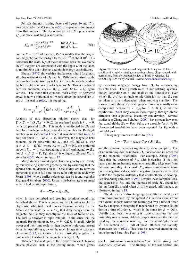
Rep. Prog. Phys. 76 (2013) 096801 P H Roberts and E M King
Perhaps the most striking feature of figures 16 and 17 ishow decisively the MS results (65b, c) separate ν-dominancefrom B-dominance. The discontinuity in the MS power ratio,f ∗ν/η, at mode switching is substantial:
f ∗ν/η =
34 (4π
2E)−2/3 for ΛΛsw,34 (4π
2E)2/3 for ΛΛsw.(65g)
For the E = 10−15 of the core, Ra∗c is smaller than the Rac of
non-magnetic convection by a factor ofE1/3 of about 105. Thisis because the scale, H ∗
c , of the convection cells that overcomethe PT theorem are comparable with the depth D of the layer,so minimizing their viscous and ohmic energy expenditures.
Eltayeb (1972) showed that similar results hold for almostall other orientations of B0 and Ω. Differences arise mainlybecause horizontal isotropy is lost, i.e. the solutions depend onthe horizontal components of B0 and/or Ω. This is illustratedhere for horizontal B0 (= B01x), with Ω (= Ω1z) againvertical. The mode that convects most easily, or preferredmode, is now a horizontal roll whose direction depends on E
and Λ. Instead of (66b), it is found that
Ra = k2
k2 − π2
(Ek4 + Λk2
x +π2k2
Ek4 + Λk2x
). (66)
Analysis of this dispersion relation shows that, forE > E1 = 1/3
√3π2 ≈ 0.02, the preferred mode is kx,c = 0,
i.e. a roll parallel to B0. This mode is unaffected by B0 andtherefore has the same large critical wave number and Rayleighnumber as in section 6.4.1 where it was shown that (62a, b)hold for small E. For E < E1 however, the magnetic fieldcounters the PT constraint and kx,c and Rac are O(1). ForΛ > Λ1(1 − E/E1) where Λ1 = 1
2
√3 ≈ 0.9, the preferred
mode is ky,c = 0, corresponding to a roll orthogonal to B0.For Λ < Λ1(1 − E/E1), the roll is oblique to B0 and Rac isgiven by (65b), shown in figure 17.
Many studies have stepped closer to geophysical realityby reintroducing spherical geometry and by assuming that theapplied field B0 depends on x. These studies are by now toonumerous to cite in full here, so we refer only to the review byFearn (1998) where earlier references can be found; see alsoZhang and Schubert (2000). Usually the basic state is assumedto be in hydrostatic equilibrium,
0 = −∇p0 + J0×B0, (67a)
which is then perturbed and growing solutions sought, asdescribed above. This is a procedure very familiar to plasmaphysicists, who find ideal modes growing rapidly on theAlfvenic time scale τA = D/VA that draw energy from themagnetic field as they reconfigure the lines of force of B0.The core is however in rapid rotation, in the sense that themagnetic Rossby number, Rom = VA/2ΩD, is small. Alfvenwaves and their time scale τA then become irrelevant; insteaddynamic instabilities grow on the much longer time scale τMS
of section 6.3.2, i.e. Coriolis forces drastically lengthen thetime needed to extract the magnetic energy of B0.
There are also analogues of the resistive modes of classicalplasma physics, such as the tearing mode, which grows
Figure 18. The effect of a zonal magnetic field B0 on the linearstability of a rapidly rotating convecting sphere. (Reproduced, withpermission, from the Annual Review of Fluid Mechanics, 32© 2000, pp 409–43 by Annual Reviews www.annualreview.org.)
by extracting magnetic energy from B0 by reconnectingits field lines. Their growth rates in non-rotating systems,though depending on η, are small on the timescale τη overwhich B0 evolves through ohmic diffusion so that B0 canbe taken as time independent when studying stability. Theresistive instabilities of a rotating system are conceptually morecomplicated because τη < τMS for Λ ∼< O(1), so that theequilibrium (67a) may evolve more rapidly through ohmicdiffusion than a potential instability can develop. Severalstudies (e.g. Zhang and Schubert (2000)) have shown, however,that zonal fields, B0 = B0(r, θ)1φ , are unstable for Λ ∼> 10.Unexpected instabilities have been reported for B0 with apoloidal part.
If buoyancy forces are added to (67a),
0 = −∇p0 + ρ0γ0αTT0r + J0×B0, (67b)
and the situation becomes significantly more complex. Theclearcut findings for the uniform B0 model above are obscuredby the magnetic instabilities. For example, Zhang (1995)finds that the decrease of Rac with increasing Λ may notreach a minimum because magnetic instability takes over frombuoyant instability. As a result, Rac may continue to decreaseeven to negative values, where negative buoyancy is neededto stop the magnetic instability that would otherwise develop.See also Zhang and Jones (1996). Despite these complications,the decrease in Rac and the increase of scale Hc, found forthe uniform B0 model when Λ is increased, still happen, asillustrated in figure 18.
The difficulty of disentangling instabilities created by Bfrom those produced by the applied ∆T is even more severefor dynamo models where flux rearranged over a time of orderτMS by a magnetic instability is regenerated by dynamo actionduring a time of order τη, which is the same for Λ = O(1).Usually (and here) no attempt is made to separate the twoinstability mechanisms. Added complications are the thermalwind uT, the magnetic wind uM, and the geostrophic wind¯ug
; see section 6.3.1. All of these influence the stabilitycharacteristics of (67b). This issue has received attention too,but is ignored here. See Fearn (1998).
6.4.3. Nonlinear magnetoconvection; weak, strong andsubcritical dynamos. The findings of the last section are
31
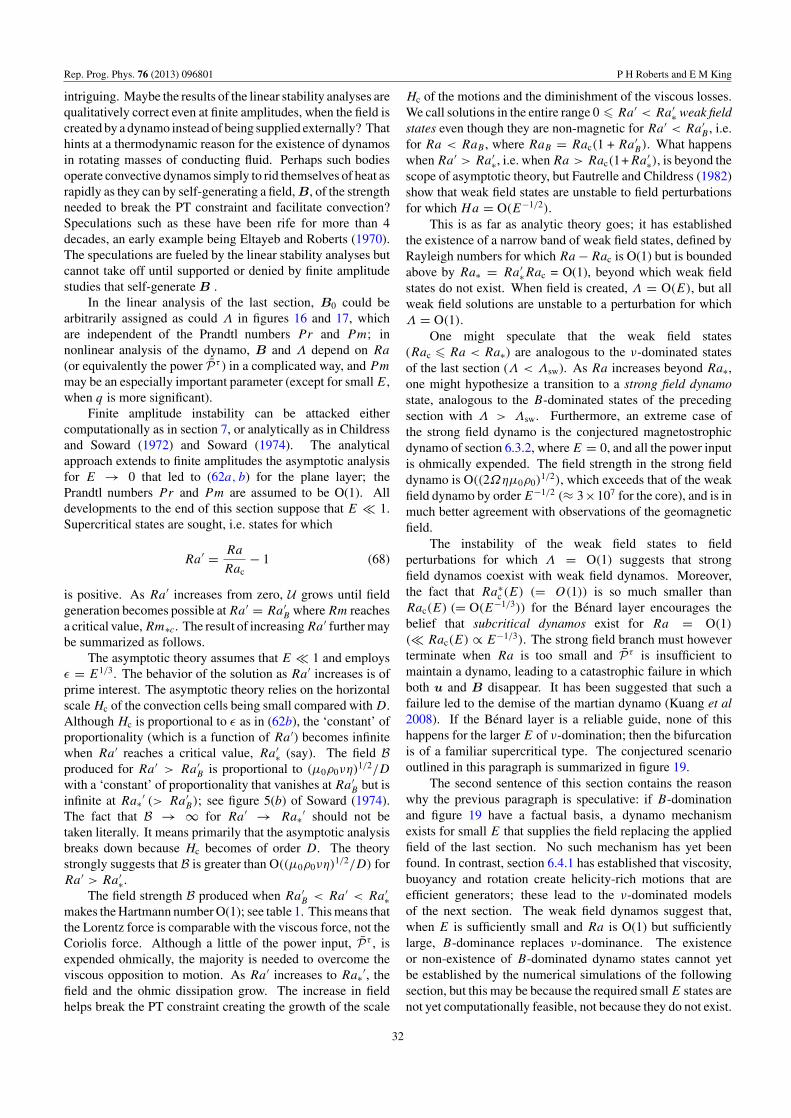
Rep. Prog. Phys. 76 (2013) 096801 P H Roberts and E M King
intriguing. Maybe the results of the linear stability analyses arequalitatively correct even at finite amplitudes, when the field iscreated by a dynamo instead of being supplied externally? Thathints at a thermodynamic reason for the existence of dynamosin rotating masses of conducting fluid. Perhaps such bodiesoperate convective dynamos simply to rid themselves of heat asrapidly as they can by self-generating a field, B, of the strengthneeded to break the PT constraint and facilitate convection?Speculations such as these have been rife for more than 4decades, an early example being Eltayeb and Roberts (1970).The speculations are fueled by the linear stability analyses butcannot take off until supported or denied by finite amplitudestudies that self-generate B .
In the linear analysis of the last section, B0 could bearbitrarily assigned as could Λ in figures 16 and 17, whichare independent of the Prandtl numbers Pr and Pm; innonlinear analysis of the dynamo, B and Λ depend on Ra
(or equivalently the power Pτ ) in a complicated way, and Pm
may be an especially important parameter (except for small E,when q is more significant).
Finite amplitude instability can be attacked eithercomputationally as in section 7, or analytically as in Childressand Soward (1972) and Soward (1974). The analyticalapproach extends to finite amplitudes the asymptotic analysisfor E → 0 that led to (62a, b) for the plane layer; thePrandtl numbers Pr and Pm are assumed to be O(1). Alldevelopments to the end of this section suppose that E 1.Supercritical states are sought, i.e. states for which
Ra′ = Ra
Rac− 1 (68)
is positive. As Ra′ increases from zero, U grows until fieldgeneration becomes possible at Ra′ = Ra′
B where Rm reachesa critical value, Rm∗c. The result of increasingRa′ further maybe summarized as follows.
The asymptotic theory assumes that E 1 and employsε = E1/3. The behavior of the solution as Ra′ increases is ofprime interest. The asymptotic theory relies on the horizontalscale Hc of the convection cells being small compared with D.Although Hc is proportional to ε as in (62b), the ‘constant’ ofproportionality (which is a function of Ra′) becomes infinitewhen Ra′ reaches a critical value, Ra′
∗ (say). The field Bproduced for Ra′ > Ra′
B is proportional to (µ0ρ0νη)1/2/D
with a ‘constant’ of proportionality that vanishes at Ra′B but is
infinite at Ra∗′ (> Ra′B); see figure 5(b) of Soward (1974).
The fact that B → ∞ for Ra′ → Ra∗′ should not betaken literally. It means primarily that the asymptotic analysisbreaks down because Hc becomes of order D. The theorystrongly suggests that B is greater than O((µ0ρ0νη)
1/2/D) forRa′ > Ra′
∗.The field strength B produced when Ra′
B < Ra′ < Ra′∗
makes the Hartmann number O(1); see table 1. This means thatthe Lorentz force is comparable with the viscous force, not theCoriolis force. Although a little of the power input, Pτ , isexpended ohmically, the majority is needed to overcome theviscous opposition to motion. As Ra′ increases to Ra∗′, thefield and the ohmic dissipation grow. The increase in fieldhelps break the PT constraint creating the growth of the scale
Hc of the motions and the diminishment of the viscous losses.We call solutions in the entire range 0 Ra′ < Ra′
∗ weak fieldstates even though they are non-magnetic for Ra′ < Ra′
B , i.e.for Ra < RaB , where RaB = Rac(1 + Ra′
B). What happenswhen Ra′ > Ra′
∗, i.e. when Ra > Rac(1+Ra′∗), is beyond the
scope of asymptotic theory, but Fautrelle and Childress (1982)show that weak field states are unstable to field perturbationsfor which Ha = O(E−1/2).
This is as far as analytic theory goes; it has establishedthe existence of a narrow band of weak field states, defined byRayleigh numbers for which Ra −Rac is O(1) but is boundedabove by Ra∗ = Ra′
∗Rac = O(1), beyond which weak fieldstates do not exist. When field is created, Λ = O(E), but allweak field solutions are unstable to a perturbation for whichΛ = O(1).
One might speculate that the weak field states(Rac Ra < Ra∗) are analogous to the ν-dominated statesof the last section (Λ < Λsw). As Ra increases beyond Ra∗,one might hypothesize a transition to a strong field dynamostate, analogous to the B-dominated states of the precedingsection with Λ > Λsw. Furthermore, an extreme case ofthe strong field dynamo is the conjectured magnetostrophicdynamo of section 6.3.2, where E = 0, and all the power inputis ohmically expended. The field strength in the strong fielddynamo is O((2Ωηµ0ρ0)
1/2), which exceeds that of the weakfield dynamo by order E−1/2 (≈ 3×10⁷ for the core), and is inmuch better agreement with observations of the geomagneticfield.
The instability of the weak field states to fieldperturbations for which Λ = O(1) suggests that strongfield dynamos coexist with weak field dynamos. Moreover,the fact that Ra∗
c (E) (= O(1)) is so much smaller thanRac(E) (= O(E−1/3)) for the Benard layer encourages thebelief that subcritical dynamos exist for Ra = O(1)( Rac(E) ∝ E−1/3). The strong field branch must howeverterminate when Ra is too small and Pτ is insufficient tomaintain a dynamo, leading to a catastrophic failure in whichboth u and B disappear. It has been suggested that such afailure led to the demise of the martian dynamo (Kuang et al2008). If the Benard layer is a reliable guide, none of thishappens for the larger E of ν-domination; then the bifurcationis of a familiar supercritical type. The conjectured scenariooutlined in this paragraph is summarized in figure 19.
The second sentence of this section contains the reasonwhy the previous paragraph is speculative: if B-dominationand figure 19 have a factual basis, a dynamo mechanismexists for small E that supplies the field replacing the appliedfield of the last section. No such mechanism has yet beenfound. In contrast, section 6.4.1 has established that viscosity,buoyancy and rotation create helicity-rich motions that areefficient generators; these lead to the ν-dominated modelsof the next section. The weak field dynamos suggest that,when E is sufficiently small and Ra is O(1) but sufficientlylarge, B-dominance replaces ν-dominance. The existenceor non-existence of B-dominated dynamo states cannot yetbe established by the numerical simulations of the followingsection, but this may be because the required small E states arenot yet computationally feasible, not because they do not exist.
32
Rep. Prog. Phys. 76 (2013) 096801 P H Roberts and E M King
Figure 19. Cartoon contrasting B-domination (left) withν-domination (right). The upward arrows mark where weak fieldsolutions terminate, and can transition to the strong field branch.The downward arrows indicate where there is insufficient power tomaintain the strong field solution, leading to catastrophic failure ofthe dynamo. Strong field solutions for Ra < Rac are termed‘subcritical’.
These difficulties and uncertainties will hopefully beresolved in the not too distant future; some progress will bereported in section 7.7.
7. Numerical simulations
Advances in computer hardware made it possible by the mid-1990s to integrate the MHD equations numerically. The firstsimulation of Glatzmaier and Roberts (1995a) did not solvethe full governing equations of the simplified cooling Earthmodel, but instead ignored the inertial acceleration terms in(43b). The governing equation for u is then diagnostic, asit was for the magnetostrophic model of section 6.3.2, andlikewise obeys a constraint, one that is more complex than(55). By taking Ro = 0, Glatzmaier and Roberts avoidedhaving to resolve the short torsional wave time scale τT; seesection 6.3.3. All subsequent numerical simulations includethe inertial force and have to resolve τT. The simulatedflows generate magnetic fields that have spatial and temporalcharacteristics consistent with the observed geomagnetic field.The geophysical promise of these early models combined withthe increasing availability of cost-effective computing powerled to a surge in numerical simulation that has continued tothis day, many of which claim to be especially Earth-like for avariety of reasons. Over time, a broadening database of modelsbecame available, permitting a systematic examination of theimpact of differences between models. The typical range ofnon-dimensional parameters occupied by most simulations islisted in table 3. As dynamo simulations proliferate, perhapsthe most important question to ask is, ‘How realistic are they?’In other words, how far can they be trusted to describe faithfullythe physics of field generation in Earth’s core? These arequestions discussed separately in part 3. Here, we presenta brief description of the simulations, focusing particularlyon how it relates to the theory laid out in sections 5 and 6.For more detailed reviews of recent numerical modeling, seeChristensen and Wicht (2007), Wicht and Tilgner (2010) andJones (2011).
Table 3. Parameters typical of numerical simulations.
Parameter Core Simulations
Input parametersE 10−15 10−3 − 10−5
Ra 1024 106–109
Pm 10−6 0.1–10Pr 0.1 0.1–10
Output parametersRm 103 40–3000Ro 10−6 10−4–1Λ O(1) 0.3–10Re 109 10–2000
7.1. Numerical methods
Section 6.1 introduced the MHD dynamo and section 6.2explicitly defined its Boussinesq form. In this section, wediscuss numerical solutions of the equations (43a–e) governingthis simplified cooling Earth model. Usually (though notinvariably), the equations are cast into equivalent though fewerequations governing Tc and the four scalars S, T , Su, Tu in thetorpol representation of B and u (see section 5.1).
The most widely-used dynamo codes time step theseequations using the pseudo-spectral method (Glatzmaier1984), which evaluates linear terms in spectral space andnonlinear terms in physical space on a spherical grid.Evaluation in spectral space means representing functionssuch as S and T by expansions, truncated to O(N2) termsby replacing = ∞ in (16g, h) by = N . In addition,the r-dependence of functions such as Sm
(r, t) and T m (r, t)
is represented by a sum of N Tchebychev functions, Tn,rescaled in r . Each time step requires a transformation fromspectral mn-space to grid rθφ-space, and vice versa. Inthe most commonly used method, m ↔ φ and n ↔ r arecarried out by fast Fourier transformations (FFT); for ↔ θ ,series over Pm
(θ) and Gaussian quadrature are used. Forsimulations in planar geometry, FFT can be employed for allthree coordinates.
Advantages of the pseudo-spectral method include itsaccuracy, the simple way it deals with (or eliminates)the pressure pe, and its easy enforcement of the dynamoconditions (18g, h). Alternatively, some simulators havechosen finite element methods to represent B, u and Tc
which enjoy the advantage of flexibility in the allocation ofspatial resolution. For a more detailed description of thesetechniques and a discussion of their strengths and weaknesses,see Christensen and Wicht (2007).
As in nearly all numerical methods, the time step dt islimited by the CFL condition (named after Courant, Friedrichsand Levy), which requires dt < u dx and dt < V
gA dx,
where dx is the grid spacing, u is the fluid velocity andV
gA is the torsional wave velocity; see (59a). This imposes
a limit on dt that is O(N−1), and makes it difficult fornumerical simulators to reproduce high Reynolds numberflows faithfully. Numerical methods exist that are not limitedby the CFL condition, for example the WENO method (e.g. Wu(2007)), but they do not circumvent the problem of inadequatenumerical resolution, as numerical diffusion arises whereverthe solution changes substantially over a few multiples of dx.
33

Rep. Prog. Phys. 76 (2013) 096801 P H Roberts and E M King
Figure 20. Schematic drawings of the α mechanism for the generation of poloidal field from toroidal field. Magnetic flux is shown asyellow ribbons, primary convective flow as black arrows, and secondary convective circulation as green arrows. See text for further details.
Figure 21. Schematic drawings of the α mechanism for the generation of toroidal field from poloidal field. Magnetic flux is shown asyellow ribbons, primary convective flow as black arrows, and secondary convective circulation as green arrows. See text for further details.
7.2. Dynamo mechanisms
In general, dynamo simulations produce self-sustainingmagnetic fields when Ra is large enough for Rm to exceeda critical value, Rmc, of about 40. Of primary interest inthe numerical models, with the magnetic curtain now drawnaside, are the detailed mechanisms by which their fieldsare generated. These mechanisms were first understood byKageyama and Sato (1997) and were visualized later in greaterdetail by Olson et al (1999) and others. Prior to the simulations,the main focus was on solutions of αω-type, as described insection 5.4.3, in which |uM|/|uφ| and |BM|/|Bφ| are small.Contrary to expectations, however, most numerical models areof α2-type; the toroidal velocity and field have much the samemagnitudes as the poloidal.
The dipolar field in the simulations is maintainedby the helicity-rich axial convection cells described insection 6.4.1. The process creating field is sometimescalled Visco–Archimedean–Coriolis (VAC) generation, sincethe flow consists of buoyantly driven convection columns withlength scales set by a balance between viscous and Coriolisforces (see section 7.6). As table 3 shows, simulations do notreach small E. Because viscosity appears in the equationsto be integrated, the ideas and terminology of the E → 0asymptotic theory of section 6 are inapplicable. There are noasymptotically thin Ekman layers in the numerical solutions,though there may be finite regions near the ICB and CMBwhere viscous forces are prominent. These can be thoughtof as analogous to Ekman layers. With this understanding,the ideas and terminology of asymptotic theory continue to beuseful.
Because VAC generation is so basic to today’s numericalmodels, it is of some interest to describe the induction processby the frozen flux theorem of section 5.2.1, where field lines areswept along with the flow and reconnect where field gradientsare large. The axial columns responsible for VAC dynamosare idealized versions of the columns that appear at the onsetof non-magnetic convection for E = O(10−4), and shown infigure 15. The inducing flow of the axial cells, u′, is periodicin φ, and we seek to picture how the mean poloidal and toroidalfields (which have respectively no and only zonal components)reinforce each other.
Figure 20 illustrates the α-effect by which poloidal fieldis produced from an initial toroidal field. We start from astate where Bφ is antisymmetric in z, being positive (west toeast) in the northern hemisphere, and negative in the southernhemisphere (figure 20(a)). The axial flow within the columns,depicted as green arrows, deflects the initial field in the axialdirection. The vorticity of each column twists these deflectedfield lines, giving them a cylindrically radial (s-) component,into and out of the page in panel b. Between the columns,reconnection occurs at the locations marked ‘R’. The vorticalcolumns continue to twist the newly made loop until it ispredominantly poloidal (panel c).
Figure 21 illustrates the mechanism by which toroidalfield is produced from an initial poloidal field by the sameidealized triumvirate of convection columns as in figure 20.The alpha effect of u′ is again responsible for field production(section 5.4.3). The initial field is Bz > 0, pictured in panel aas field ribbons between the convection columns. In panel b,these field ribbons are deflected in φ by the secondary returnflow between the columns near the equator, shown as green
34

Rep. Prog. Phys. 76 (2013) 096801 P H Roberts and E M King
arrows. The field disturbances are then swept further in φ ands by the primary rotation of the columns, as depicted in panelc, and are stretched until they reconnect in front of and behindthe columns at the locations marked ‘R’. Panel d illustrates thefinal state of this idealized process, with Bφ > 0 in front of thecolumns in the northern hemisphere and behind the columnsin the southern hemisphere, and Bφ < 0 behind the columnsin the northern hemisphere and in front of them in the southernhemisphere.
These conceptual field generation mechanisms indicatehow a dipolar field is maintained by axial convection columns.The actual field generation mechanism in the simulations,though similar, is more complicated. Reconnection of fieldlines is equally essential but is a continuous process due toohmic diffusion rather than being an abrupt failure of the frozenflux theorem; see section 5.2.2.
7.3. Dynamo regimes
Our description of the VAC mechanism in the preceding sectionis essentially a linear one in the sense that it balances theviscous and Coriolis forces, which are linear in u, with thebuoyancy force which is linear in Tc, and therefore in u for nearmarginal states. Nonlinear inertial forces become increasinglysignificant as the buoyant forcing (Ra) increases, and theconvective motions grow in amplitude and become moreirregular. When the inertial force is large enough, a transitionoccurs from dipole-dominated fields to multipolar fields.Figure 22 shows an example of field and flow from simulationsin each regime. In general, the coherent, columnar convectionmanifest near onset generates dipolar fields (figure 22, leftcolumn), and strongly driven, three-dimensional convectionproduces less coherent surface fields (figure 22, right column).(Note, however, that in some cases columnar convectiongenerates non-dipolar fields (Soderlund et al 2012).)
Christensen and Aubert (2006) showed that the Rossbynumber, Ro = U/2D, of table 1 is not the best measure ofthe inertial force to use in describing the transition. Instead,they propose maintaining the scale dependence of the inertialforce in parameterizing its effects, leading to a ‘local’ Rossbynumber, RoL = U/2LU = Ro (D/LU ), which is commonlyused in oceanographic contexts. Here, LU is the characteristicflow scale. Figure 23 shows d plotted versus RoL forthe dynamo model population studied in King et al (2010),where d is the dipolarity defined in (8c). The transitionfrom dipolar to non-dipolar field generation occurs nearRoL ≈ 0.1. In the parlance of astrophysical dynamo theory,the dipolar field generation arises from large scale dynamoaction, where LB > LU , whereas the inertially dominatedconvection operates as a fluctuating dynamo, where LB < LU .It can be seen, however that a secondary dependence on Pm
(indicated by symbol size) influences the regime transition,presumably due to its influence on the relative length scales offlow and field.
This discussion of dynamo regimes has so far focused onthe effect of varying Ra for E = O(10−4), Pm = O(1),and Pr = O(1). When pushed to more extreme values,these parameters also substantially impact the dynamics of
Rad
ial F
ield
Axi
al V
ortic
ity
Ra = 40 Ra = 4000
Figure 22. An example of the difference between dipolar (leftpanels) and non-dipolar (right panels) dynamo simulations, fromSoderlund et al (2012) with permission. The top row showsmagnetic field structures as contours of Br on the outer domainboundary, magenta and green showing positive and negative Br ,respectively. The bottom row displays flow structures as isosurfacesof axial vorticity, ζ ′
z, red (blue) being positive (negative). Bothsimulations have E = 10−4, the left with Ra = 40 and the rightwith Ra = 4000.
10−3
10−5
10−6
10−4
10−2 10−1 10 00
0.1
0.2
0.3
0.4
0.5
0.6
0.7
0.8
0.9
1
10−3
d
RoL E
stabledipoles
reversingnon-dipoles
Figure 23. Calculations of dipolarity, d, are plotted versus the localRossby number, RoL from a suite of dynamo simulations. Symbolcolors vary with E, and symbol size is proportional to log(Pm) with0.06 < Pm < 20.
the simulations. As the Ekman number is decreased to about10−6, the VAC convection columns become elongated in thes-direction into sheet-like cells, an effect first observed in thenon-magnetic laboratory convection experiments of Sumitaand Olson (2000); see figure 24(a). The simulations ofKageyama et al (2008) reached E = 5 × 10⁻⁷, at whichsheet plumes were also observed; see figure 24(b). As withthe VAC dynamo mechanism illustrated in section 7.2, thesesheets generate magnetic fields by the α-effect, though their
35

Rep. Prog. Phys. 76 (2013) 096801 P H Roberts and E M King
ba
Figure 24. Visualizations from a an experiment and b a simulationshowing the development of sheet-like plumes at small E. Theexperiment (Sumita and Olson 2000) was done in a rotatinghemisphere of water, with E = 2 × 10⁻⁶. The simulation(Kageyama et al 2008) has E = 5 × 10⁻⁷. The image shows colorcontours of axial vorticity. Image adapted from Kageyama et al(2008) with permission.
precise generation mechanism may differ from models withlarger E (Miyagoshi et al 2011).
The systematic influences of reducing Pm and Pr
to more realistic values are less well understood. Thenumerical accessibility of small values of Pm is limited bythe requirement that Rm > Rmc for dynamo action, by theresulting high values ofRe, and therefore by the CFL condition(see section 7.1). Additionally, geophysical relevance requiresthatRo = ReE 1, such that reducingPm requires thatE bereduced as well. Christensen et al (1999) observe empiricallythat the minimum value of Pm required to spur dynamo action(near convective onset) is related to the Ekman number asPmmin ≈ 450E3/4.
The effects of varying Pr are often ignored under thepresumption that turbulence standardizes effective diffusivitiessuch that ‘turbulent’ values of Pr will tend toward unity(e.g. Gubbins (2001)). Experimental evidence, however,tends to refute this notion. For example, the influenceof Pr on the dynamics of turbulent convection is foundto be significant even for very high Re (e.g. Ahlers et al2009). In addition, however, the combination of thermal andcompositional convection in the core, for which Pr < 1and Pr > 1, respectively, complicates the usual simplifyingreduction to a single buoyancy source (see section 6.2).
Despite these challenges, some modelers have addressedthe effects of fluid properties on the dynamo simulations.For example, Sreenivasan and Jones (2006) vary Pm = Pr ,finding, in general, that the dynamics are relatively insensitiveto changes in Pm = Pr above values of 0.5, but when Pm =Pr = 0.2, the relative influence of inertia becomes important.
Figure 25. A polarity reversal from the simulation of Glatzmaieret al (1999). Reprinted with permission from Macmillan PublishersLtd, copyright 1991.
Focusing on the magnetic Prandtl number, Takahashi et al(2008) observe a marked separation of characteristic scalesof magnetic and kinetic energy when Pm = 0.2 < Pr .Calkins et al (2012) utilize the computational advantages ofa non-magnetic, quasi-two-dimensional convection model toillustrate that varying Pr between 0.1 and 10 dramaticallyalters flow structures and temporal behavior.
7.4. Reversals; boundary conditions
Even the first numerical model had a solution thatspontaneously reversed its polarity; see Glatzmaier andRoberts (1995b), and figure 25. Since then many othersimulations have also reversed their fields, and considerableefforts have been made to learn more about the mechanismresponsible. For reviews specific to this topic, see Wicht et al(2009) and Amit et al (2010).
Figure 23 shows that the models generally transition tomultipolar states as RoL increases above a certain value.Although multipolar field generation is not directly relevantto the geodynamo, these solutions also exhibit chaotic polarityreversals of their weak dipole components. Interestingly, forRoL only slightly less than the transitional value, solutions canbe found that are both dipole-dominated and exhibit sporadicpolarity reversals, whereas simulations at lower or higher Ra
only exhibit one or the other. Clearly, the possibility thatthis explains spontaneous geomagnetic field reversals deservesexploration. It is called the ‘VAC reversal mechanism’ below.
It is argued in section 7.6, on the basis of simulationsfor which E > 10−6, that LU = O(E1/3D). If this resultstill holds for E = 10−15, it implies that RoL = O(105Ro),which is about 0.1 for the Ro = 10−6 of table 1. Whetherthis near transitional value supports the VAC reversal model isvery uncertain as no small E simulations exist that substantiateLU = O(E1/3D) for E = 10−15. It is equally plausible thatinstead only strong field dynamos then exist and LU = O(D).A more recent explanation of reversals sees them as a by-product of core turbulence (Petrelis et al 2009).
That dipolar, reversing dynamo simulations appear onlynear a relatively sharp boundary between the dipolar andmultipolar regimes is an unsatisfactory aspect of the VAC
36

Rep. Prog. Phys. 76 (2013) 096801 P H Roberts and E M King
reversal mechanism, as it requires the geodynamo to reside in anarrow range of RoL. The need for such a coincidence may berelaxed by different boundary conditions. In particular, mostmodels to date use fixed temperature conditions at the ICB andCMB. As mentioned in section 6.1.4, fixed heat flux boundaryconditions are more realistic for the CMB, and the results ofKutzner and Christensen (2002) suggest that they more easilypermit polarity reversals in dipole-dominated solutions.
Section 6.1.4 pointed out that, because the thermal timeconstant of the mantle is so great, the thermal boundaryconditions at the CMB can be assumed to be independent oft in studying core dynamics. Because the thermal state ofthe mantle is unlikely to depend only on r , the temperatureand heat flux at the CMB depend on θ and φ. Many differentchoices ofTc(ro, θ, φ) and IT
r (ro, θ, φ) have been explored; seethe detailed review of this topic by Wicht and Tilgner (2010).The frequency and style of reversals are affected by the choiceof thermal boundary conditions, and, interestingly, the virtualmagnetic poles sometimes follow preferred paths in longitudeduring the course of reversals in response to these boundaryconditions. See section 3.2 and also Petrelis et al (2011).
Beyond their impact on polarity reversals, laterallyheterogeneous thermal boundary conditions may also haveprofound effects on the steady state behavior of flow and field inthe models. Willis et al (2007) observed that, imposing thermalvariations at the CMB inspired by those inferred from mantletomography, steady state field and flow can become ‘locked’to the mantle in some models. This effect has been promotedas a possible explanation for two pairs of geomagnetic fluxpatches that are persistent in historical and archeomagneticfield reconstructions. Aubert et al (2008) observe that animposed CMB heterogeneity may be communicated by largescale convection patterns to the thermal boundary conditionsat the ICB, which is offered as a possible explanation forthe seismically observed anisotropy of the inner core. Moregeneral exploration of the regimes produced by laterallyvarying thermal boundary conditions are given by Davies et al(2009) and Aurnou and Aubert (2011).
Just as various thermal boundary conditions can lead toimportant differences in the dynamo solutions, so too canchanging the mechanical boundary conditions. Beginningwith Kuang and Bloxham (1997) some modelers have electedto reduce the regrettably prominent role of viscosity in themodels by permitting free slip along the boundaries. In theabsence of the frictional effect of Ekman pumping, modelswith stress-free boundaries produce more intense zonal flowsthan models with no-slip boundaries. The differential rotationof these mean flows is capable of generating strong toroidalfields by the ω-effect (e.g. Buffett and Bloxham (2002); seesection 5.4.3). Strong zonal shearing, however, is also capableof inhibiting the radial convection necessary for maintainingdipolar fields by the α-effect. Thus, although stable dipolesolutions are found, they are generally less pervasive formodels employing stress-free boundaries than those with no-slip boundaries. Parameter surveys using stress-free modelsfind a wealth of interesting non-dipolar regimes, marked bya variety of field morphologies and temporal behavior (e.g.Busse and Simitev 2006).
7.5. Inner core rotation
The Glatzmaier and Roberts (1995a) simulation treated theinner core as a solid that has the same conductivity as the outercore, and can freely rotate in response to the forces the outercore exerts on it. Previously, insofar as the angular speed,Ωi , of the inner core was contemplated at all, it was arguedto be in the same retrograde direction as the westward drift atthe Earth’s surface (section 3.2). Surprisingly, the simulationpredicted that the rotation is in the opposite, prograde sense andis 2o–3o yr−1 in magnitude. Glatzmaier and Roberts (1996a)showed that, even though their simulation had to use (as usual)an E that was much too large, the viscous torque that the outercore exerts on the inner core is negligible. The super-rotation ofthe inner core is magnetically controlled; the inner core tries torotate with the lower layers of the fluid core as in a synchronousmotor. In this way, inner core rotation tells something aboutthe movement of these layers.
This prediction about Ωi would have been only ofacademic interest had not the seismologists Song andRichards (1996) quickly realized that the inner core’slack of axial symmetry could be used to test the modelprediction. Subsequent seismological research concluded thatthe prediction, though correct in direction, overestimates itsmagnitude by about an order of magnitude (Souriau 2007). Thetoo-rapid inner core rotation predicted by numerical modelsmay be explained by their lack of gravitational coupling. Inaddition to EM torques, tidal bulging of the solid inner coreand mantle exchange gravitational torques when the bulgesare misaligned, and these gravitational torques may coupleinner core and mantle more effectively than magnetic torques(Buffett and Glatzmaier 2000). The models, however, treatthe ICB and CMB as spheres, permitting no gravitationalcoupling across the fluid core. When gravitational couplingis re-instated, the prograde inner core rotation rate is reducedby about an order of magnitude, in apparent agreement with thelater seismological results. Recently Tkalcic et al (2013) findΩi ≈ 0.25 − 0.48o yr−1, with additional decadal fluctuationof order 1o yr−1 see also Roberts and Aurnou (2013).
The discussion of core convection within this articlefocuses predominantly on that occurring outside of the TC,which only encounters the inner core at its equator. Flowswithin the TC, however, sweep across the full extent of theICB. Due to its distinct geometry, it is generally thoughtthat a thermal wind balance (51) in the TC leads to largescale vortical flow there, with upwellings along the rotationaxis, prograde zonal flow near the ICB, and retrograde zonalflow near the CMB (e.g. Aurnou et al (2003)). Such flowstructures are invoked to explain both the inner core super-rotation, as well as a polar vortex beneath the northernhemisphere CMB inferred from geomagnetic secular variation(Olson and Aurnou 1999). Thus, in addition to geomagneticobservations, recent developments permit useful informationabout conditions far beneath the CMB to be extracted frommeasurements of inner core rotation. More importantly, itallows core dynamics to be observed derived directly fromseismology. See the review by Deguen (2012).
37

Rep. Prog. Phys. 76 (2013) 096801 P H Roberts and E M King
Figure 26. Characteristic length scale of flow, LU/D, from numerical dynamo simulations plotted versus E and Λ. Symbol colors illustratevalues of Λ in panel a and E in panel b. The solid line in panel a shows LU = 5E1/3D.
7.6. Scaling
Since the simulations are incapable of reaching the parametersnecessary for true dynamic similarity with the geodynamo, weturn to scaling analysis. The goal of such analysis is powerlaw scaling relationships, which depict the general behaviorof one parameter with respect to others within a particulardynamical regime. Theoretical scaling laws can be built onreductive assumptions regarding a system’s physics; testingsuch scaling analysis against observations or model outputsgives information about the quality of those assumptions. Forexample, in section 6.4, the scaling behavior of the criticallength scale (Hc) and Rayleigh number (Rac) for the onset ofconvection is portrayed for three distinct dynamical regimes.Focusing on the scaling behavior of Hc, they are: Hc ≈ D fornon-magnetic (Λ = 0), non-rotating (E−1 = 0) convection;Hc ∝ E1/3D for rapidly rotating (E → 0), non-magnetic(Λ = 0) convection; and Hc ∝ Λ−1/2D for magnetostrophicE → 0, Λ = O(1)) convection. Assuming that these criticalwavelengths persist beyond onset, the latter two scalingsillustrate the stark contrast between the asymptotic structure ofconvection with and without a magnetic field present. WhenB = 0, it seems possible from section 6.4 that more than onepower law regime will emerge as E → 0, and such regimetransitions must be taken into consideration when developingand extrapolating scaling laws.
Figure 26 shows a test of these predicted critical lengthscales against results from a suite of dynamo simulationscarried out by Christensen and Soderlund (reported in Kinget al (2010)). The numerical model follows the method laidout in section 7.1, and all 159 individual simulations employno-slip, isothermal boundaries. Characteristic length scales ofconvection are calculated as the inverse of the mean azimuthalwavenumber of kinetic energy, LU = πD〈u2〉/∑
m〈u2m〉,
where um is the velocity of azimuthal mode m. Figure 26(a)shows calculations of LU plotted againstE. In it, the scaling forcritical perpendicular wavelengths in non-magnetic, rotatingconvection, LU ∝ E1/3D, is shown as the solid line. Similarly,figure 26(b) shows LU versus Λ. Figure 26(a) shows ratherclearly that in this broad array of dynamo simulations, thecharacteristic length scales of convection follow the non-magnetic scaling, LU ∝ E1/3D, regardless of magnetic fieldstrength. This observation indicates that viscosity is primarilyresponsible for breaking the Proudman–Taylor constraint, and
magnetic fields do not strongly affect convection in the models,despite having Λ 1 in most cases. Soderlund et al (2012)switch off the magnetic fields in a subset of these dynamos,and observe that the dynamical influence of magnetic fieldson convection is indeed weak. The ramifications of theweak influence of Lorentz forces in these dynamo models isdiscussed further in section 9.1.
7.6.1. Flow speeds. Several different scaling laws for the rmsflow speeds have been proposed, most of which are reviewedby Christensen (2010) and Jones (2011). Three differentpublished scaling laws, in particular, are referred to as theMAC, CIA, and VAC balance scalings, after the triple forcebalance on which they are based, where ‘C’ stands for Coriolis,‘A’ for Archimedean’, referring to the buoyancy force, ‘M’ for‘magneto’, referring to the Lorentz force, ‘I’ for inertial, and‘V’ for viscous. By focusing on just three forces, these scalinglaws exclude other possible balances, as for example in theVAC reversal model of section 7.4 which requires four forcesin its description: VAC and I.
The CIA scaling has a different character from VAC andMAC scalings in that C and I are conservative forces, leavingthe energy input from A unbalanced. Even though the viscousforce may be smaller than C, I and A forces, the CIA forcebalance may apply to strongly driven, non-magnetic systems,the A power input being carried by the turbulent cascade of I tosmall wavelengths where it is dissipated by V. Cascade impliesthat the kinetic Reynolds number, Re (∼ I/V ), is large, whichconfirms that V is unimportant at large length scales. SinceRe = Ro/E, this also means that E Ro, which agrees withour estimates of E and Ro; see table 1. For magnetic systems,the situation can be radically different. The CIA concept wouldrequire the I force to be much greater than M, i.e. VA/U 1,where VA is the Alfven velocity (B/
√(µ0ρ0)). However,
the estimates of table 1 contradict this, giving VA/U ≈ 70.It appears therefore that the CIA force balance may not begeophysically relevant. Because of the small magnetic Prandtlnumber of the core, it is more plausible that A is ohmicallydissipated locally without cascade, and that the force balanceis closer to MAC than to CIA; see section 9.2. The viscousdomination and magnetic domination scenarios contrasted insection 6 are then best studied through VAC and MAC balancesnot involving I.
38

Rep. Prog. Phys. 76 (2013) 096801 P H Roberts and E M King
Figure 27. A comparison of flow speed scaling law (69c) withcalculations from dynamo simulations. Dimensionless rms flowspeeds, Re, are plotted versus RaPr−1(D/LU ). Symbol colorsillustrate Prandtl number values from the simulations. The solid lineshows Re = 0.02RaPr−1(D/LU ).
All three scalings share a balance between Coriolis andbuoyancy forces, which in the vorticity equation (45) is referredto as the thermal wind balance (see (51a)):
− 2Ω · ∇u = γ0αT∇Tc×r. (69a)
The Proudman–Taylor theorem (49b) indicates that axialgradients in u are small, so that we scale the Coriolis termas 2Ω · ∇u ∼ 2U/D. Assuming that thermal gradientsare commensurate with characteristic flow scales LU , we takethe buoyancy term to scale as γ0αT∇Tc×r ∼ αTg0∆Tc/LU .Thus, we can estimate the rms flow speed as
U ∼ αTg0∆TcD
2LUor Re ∼ Ra Pr−1 D
LU, (69b, c)
where the Reynolds number Re = UD/ν is the dimensionlessflow speed.
Figure 27 shows calculations of Re from the dynamosimulations plotted versus the thermal wind balance scaling(69c). The data are reasonably well described by thepredicted scaling, although a secondary dependence on Pr
(denoted by symbol colors) is apparent. For extrapolationto the geodynamo and other planets, where ∆Tc is poorlyconstrained, (69a) is multiplied by U , and it is assumed thatUγ0αT∇Tc×r ∼ γ0αT∇×(Tcr · u) ∼ Pτ /(ρ0LUD
3), wherePτ is the total buoyant power input (47c). The flow speedscaling can then be written as
U ∼(
Pτ
2ρ0LUD2
)1/2
or Re ∼(
C E D
LU
)1/2
,
(69d, e)
where
C = PτD
ρ0ν3= Ra(Nu − 1)E−1Pr−2 (69f )
is a dimensionless convective power parameter.The difference between the MAC, CIA, and VAC scalings
originate in their separate treatments of the length scale LU ,
which are determined by the third force in each triple balance.They are
LU ∼ D, LU ∼ Ro1/2D and LU ∼ E1/3D,
(69g, h, i)
respectively for the MAC, CIA, and VAC balances. The MACbalance length scale assumes that a magnetostrophic dynamowill experience a relaxation of the Proudman–Taylor constraintthrough the Lorentz force, following the ideas outlined insection 6.4.2 (Starchenko and Jones 2002). The CIA balancelength scale is known as the Rhines scale, the length scaleat which the inertial term balances the Coriolis term in thevorticity equation (Hide 1974). The VAC balance scalingis the length scale at which the viscous and Coriolis termsbalance in the vorticity equation, and also corresponds to thecritical wavenumber scaling for the onset of non-magneticrotating convection shown in section 6.4.1. Although, withinthe parameter range accessed by the simulations, these threescaling laws are not very different, the observation that thecharacteristic length scales are well described by (69i) (seefigure 26(a)) seems to indicate that the simulations are closestto being in VAC balance (e.g. King and Buffett (2013)).
Christensen and Aubert (2006) derive another, empiricalscaling of the flow speeds using a database of simulations verysimilar to that used in deriving figure 27. They assume that thedynamics within the models are independent of all diffusivities,and develop a set of dimensionless parameters reflecting thisassumption. There is very little evidence, however, that thedynamics in the models, or even the core, are or should bediffusionless. Evidence to the contrary abounds. For example:magnetic diffusion plays a critical role in field generationthrough reconnection (section 5.2.2); diffusive boundary layershave been shown to be important in the establishment of globaldynamics (King et al 2009, 2010); varying Prandtl numberscan substantially alter convection dynamics (e.g. Aubert et al(2001); Calkins et al (2012)); and the LU ∼ E1/3D scalingshown in figure 26(a) indicates that, within these simulations,the Proudman–Taylor constraint is broken by viscosity actingon the small length scales perpendicular to Ω.
The extrapolation of flow speed scalings (69) to the coreis complicated by the fact that no well constrained estimateof LU exists. The simulations predict that LU ≈ E1/3D
(see figure 26(a)), but it is generally thought that Lorentzforces, rather than viscosity, will break the Proudman–Taylorconstraint as E → 0, possibly leading to the large scaleflow expected for magnetostrophic convection (69g). Since Ucan already be constrained by secular variation observations(10f ), we may instead use (69d) to estimate LU . TakingU = 0.4 mm s−1, Pτ = 0.2 TW (see section 6.2.1), and theremaining quantities from table 1, we have LU ≈ 2 × 10⁵ m,a value which supports the existence of a MAC balance inthe core (Starchenko and Jones 2002). If, instead, we usethe viscous scaling (69i), which predicts a core value ofLU ≈ 50 m, we have U ≈ 20 mm s−1, a value that far exceedsestimates from geomagnetic secular variation.
7.6.2. Magnetic field strength. Section 5 shows that, ifdriven by a steady velocity, the field of a successful kinematic
39

Rep. Prog. Phys. 76 (2013) 096801 P H Roberts and E M King
dynamo grows from a small seed to become exponential intime, as in (13a, b). In nonlinear dynamos, such as the dynamosimulations, Lorentz forces increase with field strength B untilthey modify the flow and saturate field growth. An importantquestion is, ‘What sets the field strength at which dynamossaturate?’ Analysis of the scaling behavior of time-averagedmagnetic energy in the dynamo simulations helps to answerthis question. Again, Christensen (2010) and Jones (2011)give more detailed reviews.
The stability theory of section 6.4.2 suggests that thecombined action of Lorentz and Coriolis forces promoteconvection, so that the dynamo may naturally ‘select’something akin to magnetostrophic balance. That is, fieldgrowth saturates when Lorentz and Coriolis forces are inbalance, since a field that is more or less intense would inhibitconvection. This hypothesis suggests that B equilibrateswhen either the Elsasser number Λ or the dynamic Elsassernumber Λd (see section 6.3.2) is of unit order. The results ofsection 7.6.1 indicate, however, that the simulations are notmagnetostrophic. Soderlund et al (2012) calculate explicitlythe ratio between Lorentz and Coriolis forces, finding that thelatter is always stronger in dipolar dynamos. This ratio offorces is well represented by Λd, which is always smaller thanunity in the simulations included in section 7.6.1, and does notappear to saturate at any preferred value. Thus, the strength ofthe Coriolis force alone does not seem to be selecting B in thesimulations.
Christensen and Aubert (2006) argue that the totalmagnetic energy may instead be limited by the power availableto offset ohmic losses. The steady power budget (47g) can bewritten as
Qτη = fη Pτ , (70a)
where we recall that Qη is ohmic dissipation, P is the totalconvective power input, and fη is the mean fraction of totalavailable power that is dissipated ohmically. In the core, it isexpected that fη ≈ 1 since the alternative form of dissipation,viscous, is likely negligible, primarily becausePm 1. In thesimulations, however, this dissipation fraction can be directlycalculated and typically falls in the range 0.2 fη 0.8, andso is maintained in the development of the scaling laws. Theleft-hand side of (70a) can be scaled as µ0ηJ 2Vo, as in (15),and using Ampere’s law (2a), we can scale the characteristiccurrent density as J ∼ B/µ0LB , such that
B2 ∼ fη
µ0PτL2B
ηD3. (70b)
As in section 7.6.1, one must treat the characteristic lengthscale, in this case LB , as the typical length scale for magneticfield variations. Section 5.2.2 points out that the expulsionof magnetic flux tubes by vortical flow gives rise to fieldscales of LB ∼ Rm−1/2D. Figure 28 shows calculations ofLB(= πD〈B2〉/∑
m〈B2m〉) plotted versus Rm. The solid
line shows LB ∝ Rm−1/2D, supporting this general scaling,but we also notice a secondary dependence on field strengthitself; symbol colors indicate values of Λ.
Assuming that LB = Rm−1/2D, (70b) becomes (24),which by (69f ) can be written in dimensionless form as
Ha2 ∼ fηC q2 Rm−1, (70c)
Figure 28. Characteristic length scales of magnetic field variations,LB/D, plotted versus the magnetic Reynolds number. The solid lineshows LB/D = 3Rm−1/2. Symbol colors indicate logarithmicvariations in Λ.
Figure 29. Dimensionless magnetic energy, Ha2, plotted versusfηCPm2Rm−1. The solid line shows Ha2 = 0.2fηCPm2Rm−1.Symbol colors indicate the fraction of input power that is dissipatedohmically, fη.
where we recall that Ha = BD/(ρ0µ0ην)1/2 is the Hartmann
number, and q = κ/η is the diffusivity ratio (see table 1).Figure 29 shows a test of scaling (70c) against calculationsfrom the dynamo simulations, and proportionality is indicatedby the solid line. The general agreement between thescaling (70c) and the simulation data indicates that the strengthof magnetic fields produced by the models may be determinedby the convective power available to Lorentz work andultimately ohmic dissipation. We notice, however, that muchof the variation in magnetic energy, represented by Ha2, canbe accounted for by changes in fη, as indicated by the colorscale. Although it is expected that fη → 1 for Pm → 0, theactual behavior of the dissipation fraction is more complicatedwithin the range of computationally accessible parameters. Noclear scaling for this important term has emerged; in fact, onecannot even say that fη clearly increases as Pm is decreased!
Interestingly, (70c) includes no explicit dependence onthe rotation rate. Presumably, the effect of the Coriolis
40

Rep. Prog. Phys. 76 (2013) 096801 P H Roberts and E M King
force may be implicitly included in its influence on U .Christensen and Aubert (2006) use the CIA scaling for U(section 7.6.1) in (70c), which incorporates a weak, butexplicit, -dependence in the magnetic field strength scaling.
7.7. Taylorization and hints of magnetostrophy
Much of sections 6.3 and 6.4 is devoted to B-dominateddynamos of MAC type. The underlying mathematics isasymptotic theory for E → 0, which is appropriate for thegeodynamo for which E ≈ 10−15 (table 1). Subcritical, strongand weak field dynamos were considered, but the asymptoticsof only the weak field dynamos has so far been unequivocallyestablished. The present section 7 has focussed mainly onnumerical dynamos, which are ν-dominated and of VAC type.Many simulations employ E so large that it is sometimesdoubted whether they represent the geodynamo adequately.Despite this general tendency, some simulations for small Eoffer hints that a strong field dynamo may not be far off, andwe briefly highlight a few of these studies here.
Sections 6.4.1 and 6.4.2 show how dramatically differentare the length scales of convection depending on whether theProudman–Taylor constraint is released by viscous or Lorentzforces, and in section 7.6 we analyze typical length scales ofconvection in dynamo models as a simple tell-tale for the forcebalance at work. Stellmach and Hansen (2004) utilize thecomputational efficiency of cartesian geometry to reach smallEkman numbers, and analyze the structure of flow in moredetail. Such box dynamos with E = 5×10⁻⁷ exhibit a jump tolarge scale convection relative to corresponding non-magneticsimulations, indicating the emergence of magnetic relaxationof the PT constraint.
Although the low E value of Stellmach and Hansenhas proven more difficult to reach in spherical shell dynamosimulations, recent modelers have observed the emergence oflarge scale flows by changing the thermal boundary conditionsfrom isothermal (44c, d) to fixed flux in simulations withE = 10−6 (Sakuraba and Roberts 2009). Subsequent work(Takahashi and Shimizu 2012) shows that this relaxation ofthe usual, small-scale columnar convection does not occur inthe absence of magnetic fields, but rather this transition tolarge scale convection occurs only in simulations with bothflux based boundary conditions and dynamo action. Thisobservation indicates that the role of Lorentz forces is critical tothe relaxation of small convective scales, and may therefore belinked to the emergence of magnetostrophy. The relationshipbetween thermal boundary conditions and magnetic fields isnot, however, well understood.
In the hunt for the subcritical dynamos discussedin section 6.4.3, Sreenivasan and Jones (2011) combinenumerical simulations with asymptotic analysis. They findthat the Lorentz force of a strong dipolar field can enhance thehelicity of convective flow near its onset, when the initial fieldis a strong dipole rather than a weak, disorganized seed field.Dynamo action is observed for Rm < Rm∗
c , where Rm∗c is
the critical magnetic Reynolds number for kinematic dynamoaction when Ra is increased from zero. In other words, astrong dipolar field can encourage dynamo action that may not
be possible if only a small seed field is present, i.e. the dynamois subcritical in the sense defined in section 6.4.3. This resultillustrates how Lorentz forces may promote dynamo action,and furthermore helps explain the propensity for stable, dipolarfield generation by rotating convection near onset.
Another signature of the magnetostrophic dynamo are thetorsional oscillations discussed in section 6.3.3. Torsionaloscillations, like magnetic relaxation, have mostly eludedmodelers. Some numerical studies quantify how closelyTaylor’s constraint is, or is not, satisfied using a ‘taylorizationparameter,’ defined by
Ta =∫Vc
(J×B)φd3x
/ ∫Vc
∣∣(J×B)φ∣∣d3x. (71)
Most simulations have Ta 0.4. Wicht and Christensen(2010) investigate the zonal motions of geostrophic cylindersC(s) for several models with E 1.5 × 10⁻⁶. Threeof their simulations have Ta < 0.2 and display torsionaloscillations that cross the shell in time τT (see table 2). Thisobservation provides further evidence that the Taylor state andmagnetostrophic dynamo may yet emerge as E is decreased toand beyond the current limits set by computational capabilities.
In section 9, we return to the issue of numerical dynamosimulations and their frontiers.
8. Laboratory experiments
The computer simulations highlighted in the precedingsection 7 successfully generate magnetic fields with simplifiedyet appropriate forcing mechanisms. They spectacularly failhowever to reach the geophysical reality of E = 10−15
and Pm = 10−6. As table 3 showed, E > 10−5 andPm > 0.1 is more typical of simulations, which thereforegrossly enhance the role of viscosity (see also section 9). Thelarge E in simulations is such a serious shortcoming that ittends to hide the no less important deficiency of large Pm.This particular shortcoming is totally avoided in laboratoryexperiments, where real liquid metals adequately representcore fluid and its Pm.
The very small magnetic Prandtl numbers of liquid metals,such as that constituting Earth’s outer core, have physicalrepercussions for the geodynamo problem. Dynamo actionrequires that Rm > O(10). The fluid Reynolds numberRe = Rm/Pm must then reach O(106) for field generation.The transition to turbulent flow usually occurs when 103 Re 104, a range rarely (and then, barely) sampled bynumerical simulation. Dynamo action in the computations ispossible only because the fluids of the simulations are endowedwith unrealistically high electrical conductivities, Pm = O(1).Real liquid metals (Pm 10−5), however, must generatemagnetic fields within fully developed turbulent flows.
Turbulence plays an important role in the generationof Earth’s magnetic field, and we shall come back to thatrole in greater detail in section 9. In the mean fieldtheory of section 5.4.2, two influences of turbulence on fieldgeneration are identified: the α-effect, whereby small-scaleflow correlations associated with the helicity of the turbulence
41

Rep. Prog. Phys. 76 (2013) 096801 P H Roberts and E M King
create large scale field; and the β-effect, whereby randomsmall-scale motions effectively diffuse large scale fields away.As Re increases, the β-effect becomes more important, to suchan extent that even the very possibility of dynamo action hasbeen questioned for Pm 1 (Schekochihin et al 2005)!
In section 8.1, we briefly review experimental studies ofdynamo action. These experiments employ realistic materialproperties and inherently ‘resolve’ turbulence, giving them adistinct advantage over numerical simulations in approachingcore values of Pm and Re. But they ignore Coriolis forcesand are kinetically driven in unrealistic domain geometries.Buoyancy is an inefficient driving force and so, to reach therequired Rm values for dynamo action, experimentalists driveflows with pumps and motors. These do not however naturallycreate flows that favor dynamo action, as convective motionsdo under the influence of rotation. Geometrical constraints arethen often imposed to promote flows proven (see section 5.3) toencourage field generation. No successful dynamo experimentto date has incorporated strong Coriolis forces.
These dynamo experiments focus on the inductionof magnetic field (11a), and sacrifice realistic core fluiddynamics (43a–c). Another class of laboratory experimentsdo the opposite: forgoing the goal of self-sustained fieldgeneration, they investigate the remaining aspects of core fluiddynamics presented in section 6, such as convection, rotationaldynamics, turbulence in the presence of magnetic fields, aswell as other dynamics and their various combinations. Anincomplete review of these core flow experiments is given insection 8.2.
8.1. Dynamo experiments
8.1.1. Kinematic dynamo experiments. Before discussingMHD dynamo experiments, we should first briefly mentionthat the first experiment to verify Bullard’s conjecture thata simply-connected conductor can produce self-sustainingmagnetic fields was reported in Lowes and Wilkinson (1963).Modeled after the Herzenberg kinematic dynamo model (seesection 5.3.1), the experiment consists of two identical, solid,iron-alloy cylinders with a radius of 3.5 cm embedded withina solid block of the same metal. The axes of the cylindersare perpendicular and separated in the direction orthogonal toboth axes by 8 cm. Remembering that the magnetic Reynoldsnumber, Rm, is not only proportional to σ but also to thepermeability µ, Lowes and Wilkinson improved the prospectsfor regeneration by using ferromagnetic materials. Theirexperiment produces spontaneous dynamo action when therate at which the cylinders are rotated exceeds some criticalvalue of order 1000 rpm. The experiment generates steadyand oscillating quadrupolar fields with intensities up to 1 mT.Subsequent experimental designs demonstrate increasinglysubtle dynamic behavior, including magnetic polarity reversals(Lowes and Wilkinson 1968). Though titled ‘laboratoryexperiments of the geomagnetic dynamo’, these experimentsignore the fluid nature of the geodynamo.
8.1.2. First generation MHD dynamo experiments. In 2000,two liquid sodium laboratory experiments reported production
of MHD dynamo action for the first time. They are the Riga andKarlsruhe dynamo experiments (Gailitis et al 2000, Stieglitzand Muller 2001), and their collective results are reviewedin Gailitis et al (2002). In both experiments, large volumesof sodium are pumped through flow channels that constrainflow to mimic theoretical kinematic dynamo models. Sodiumis the fluid of choice for nearly all MHD dynamo experimentsbecause of its relatively low density (ρ ≈ 103 kg m−3) and highelectrical conductivity (η ≈ 0.1 m2 s−1). For a more detailedreview of these two experiments, see Gailitis et al (2003).
The Riga dynamo experiment, shown in figure 30(a),is designed after the Ponomarenko dynamo model (seesection 5.3.2). In the experiment, a schematic of which isshown in figure 30(a), three concentric cylindrical vessels of3 m length are filled with liquid sodium. Downward, helicalflow is produced at the top of the innermost cylinder by animpeller driven by a motor at more than 100 kW. At the oppositeend, guide vanes remove mean vorticity from the flow as itexits to the second cylinder to continue back upward as anaxial return flow. The outermost cylinder holds sodium at rest,to increase the total magnetic diffusion time of the models(Bullard and Gubbins 1977). Above Rm ≈ 20 (based on theradius of the inner cylinder), oscillating magnetic fields of tensof mT are produced and sustained for several hundred diffusiontimes (Gailitis et al 2003).
The Karlsruhe dynamo experiment was designed afterthe Roberts dynamo model (see section 5.3.3). Shown infigure 30(b), the experiment consists of fifty-two 1 m long,10 cm wide flow channels that are arranged in a cylindricalarray ∼2 m diameter wide. Each channel is comprised of twoconcentric regions: an inner pipe, and an outer counterflowpipe fitted with helical baffles that impart helicity to the flow.The channels are interconnected at each end and sodium ispumped through the channel array by three external magneticpumps driven at up to 200 kW. Beyond a critical flow rate, theapparatus generates stationary magnetic fields of up to severalhundred gauss, sustained for more than an hour. The largescale structure of the field is that of a dipole whose axis isperpendicular to the helical flow channels (Muller et al 2006).
Both the Riga and Karlsruhe experiments are unstableto dynamo action near their (relatively low) critical magneticReynolds number, Rmc, calculated from their purely kinematiccounterparts. That the observed Rmc is not markedlyincreased despite having Re 1 indicates that the small-scaleturbulence in these laboratory dynamos does not significantlyenhance the effective diffusion of magnetic field. Thisabsence of a substantial β-effect in the Riga and Karlsruhedynamo experiments is attributed to the particular flow pathsenforced. In the Karlsruhe dynamo experiment, for example,the constrained helical flow channels limit turbulent velocityfluctuations to less than 10% of the mean flow.
8.1.3. Turbulent dynamo experiments. Third generationdynamo experiments seek to improve on the geophysicalrelevance of the Riga and Karlsruhe dynamos by investigatingfield generation in unconstrained domains. These experiments,however, find dynamo action more elusive.
42
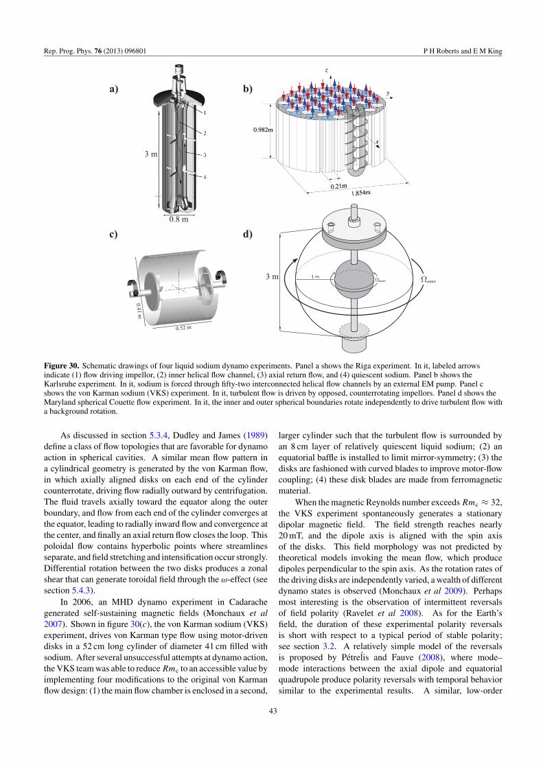
Rep. Prog. Phys. 76 (2013) 096801 P H Roberts and E M King
0.8 m
3 m
0.52 m
0.41 m
outerinner3 m
a) b)
c) d)
Figure 30. Schematic drawings of four liquid sodium dynamo experiments. Panel a shows the Riga experiment. In it, labeled arrowsindicate (1) flow driving impellor, (2) inner helical flow channel, (3) axial return flow, and (4) quiescent sodium. Panel b shows theKarlsruhe experiment. In it, sodium is forced through fifty-two interconnected helical flow channels by an external EM pump. Panel cshows the von Karman sodium (VKS) experiment. In it, turbulent flow is driven by opposed, counterrotating impellors. Panel d shows theMaryland spherical Couette flow experiment. In it, the inner and outer spherical boundaries rotate independently to drive turbulent flow witha background rotation.
As discussed in section 5.3.4, Dudley and James (1989)define a class of flow topologies that are favorable for dynamoaction in spherical cavities. A similar mean flow pattern ina cylindrical geometry is generated by the von Karman flow,in which axially aligned disks on each end of the cylindercounterrotate, driving flow radially outward by centrifugation.The fluid travels axially toward the equator along the outerboundary, and flow from each end of the cylinder converges atthe equator, leading to radially inward flow and convergence atthe center, and finally an axial return flow closes the loop. Thispoloidal flow contains hyperbolic points where streamlinesseparate, and field stretching and intensification occur strongly.Differential rotation between the two disks produces a zonalshear that can generate toroidal field through the ω-effect (seesection 5.4.3).
In 2006, an MHD dynamo experiment in Cadarachegenerated self-sustaining magnetic fields (Monchaux et al2007). Shown in figure 30(c), the von Karman sodium (VKS)experiment, drives von Karman type flow using motor-drivendisks in a 52 cm long cylinder of diameter 41 cm filled withsodium. After several unsuccessful attempts at dynamo action,the VKS team was able to reduceRmc to an accessible value byimplementing four modifications to the original von Karmanflow design: (1) the main flow chamber is enclosed in a second,
larger cylinder such that the turbulent flow is surrounded byan 8 cm layer of relatively quiescent liquid sodium; (2) anequatorial baffle is installed to limit mirror-symmetry; (3) thedisks are fashioned with curved blades to improve motor-flowcoupling; (4) these disk blades are made from ferromagneticmaterial.
When the magnetic Reynolds number exceeds Rmc ≈ 32,the VKS experiment spontaneously generates a stationarydipolar magnetic field. The field strength reaches nearly20 mT, and the dipole axis is aligned with the spin axisof the disks. This field morphology was not predicted bytheoretical models invoking the mean flow, which producedipoles perpendicular to the spin axis. As the rotation rates ofthe driving disks are independently varied, a wealth of differentdynamo states is observed (Monchaux et al 2009). Perhapsmost interesting is the observation of intermittent reversalsof field polarity (Ravelet et al 2008). As for the Earth’sfield, the duration of these experimental polarity reversalsis short with respect to a typical period of stable polarity;see section 3.2. A relatively simple model of the reversalsis proposed by Petrelis and Fauve (2008), where mode–mode interactions between the axial dipole and equatorialquadrupole produce polarity reversals with temporal behaviorsimilar to the experimental results. A similar, low-order
43
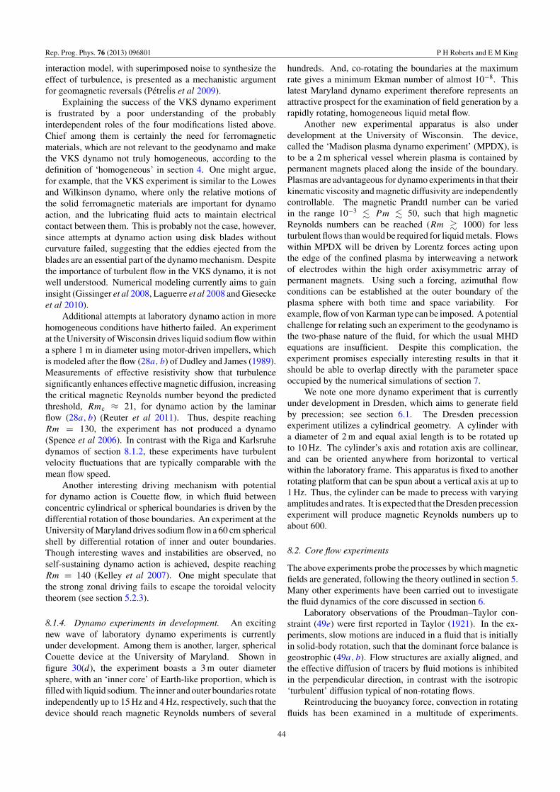
Rep. Prog. Phys. 76 (2013) 096801 P H Roberts and E M King
interaction model, with superimposed noise to synthesize theeffect of turbulence, is presented as a mechanistic argumentfor geomagnetic reversals (Petrelis et al 2009).
Explaining the success of the VKS dynamo experimentis frustrated by a poor understanding of the probablyinterdependent roles of the four modifications listed above.Chief among them is certainly the need for ferromagneticmaterials, which are not relevant to the geodynamo and makethe VKS dynamo not truly homogeneous, according to thedefinition of ‘homogeneous’ in section 4. One might argue,for example, that the VKS experiment is similar to the Lowesand Wilkinson dynamo, where only the relative motions ofthe solid ferromagnetic materials are important for dynamoaction, and the lubricating fluid acts to maintain electricalcontact between them. This is probably not the case, however,since attempts at dynamo action using disk blades withoutcurvature failed, suggesting that the eddies ejected from theblades are an essential part of the dynamo mechanism. Despitethe importance of turbulent flow in the VKS dynamo, it is notwell understood. Numerical modeling currently aims to gaininsight (Gissinger et al 2008, Laguerre et al 2008 and Gieseckeet al 2010).
Additional attempts at laboratory dynamo action in morehomogeneous conditions have hitherto failed. An experimentat the University of Wisconsin drives liquid sodium flow withina sphere 1 m in diameter using motor-driven impellers, whichis modeled after the flow (28a, b) of Dudley and James (1989).Measurements of effective resistivity show that turbulencesignificantly enhances effective magnetic diffusion, increasingthe critical magnetic Reynolds number beyond the predictedthreshold, Rmc ≈ 21, for dynamo action by the laminarflow (28a, b) (Reuter et al 2011). Thus, despite reachingRm = 130, the experiment has not produced a dynamo(Spence et al 2006). In contrast with the Riga and Karlsruhedynamos of section 8.1.2, these experiments have turbulentvelocity fluctuations that are typically comparable with themean flow speed.
Another interesting driving mechanism with potentialfor dynamo action is Couette flow, in which fluid betweenconcentric cylindrical or spherical boundaries is driven by thedifferential rotation of those boundaries. An experiment at theUniversity of Maryland drives sodium flow in a 60 cm sphericalshell by differential rotation of inner and outer boundaries.Though interesting waves and instabilities are observed, noself-sustaining dynamo action is achieved, despite reachingRm = 140 (Kelley et al 2007). One might speculate thatthe strong zonal driving fails to escape the toroidal velocitytheorem (see section 5.2.3).
8.1.4. Dynamo experiments in development. An excitingnew wave of laboratory dynamo experiments is currentlyunder development. Among them is another, larger, sphericalCouette device at the University of Maryland. Shown infigure 30(d), the experiment boasts a 3 m outer diametersphere, with an ‘inner core’ of Earth-like proportion, which isfilled with liquid sodium. The inner and outer boundaries rotateindependently up to 15 Hz and 4 Hz, respectively, such that thedevice should reach magnetic Reynolds numbers of several
hundreds. And, co-rotating the boundaries at the maximumrate gives a minimum Ekman number of almost 10−8. Thislatest Maryland dynamo experiment therefore represents anattractive prospect for the examination of field generation by arapidly rotating, homogeneous liquid metal flow.
Another new experimental apparatus is also underdevelopment at the University of Wisconsin. The device,called the ‘Madison plasma dynamo experiment’ (MPDX), isto be a 2 m spherical vessel wherein plasma is contained bypermanent magnets placed along the inside of the boundary.Plasmas are advantageous for dynamo experiments in that theirkinematic viscosity and magnetic diffusivity are independentlycontrollable. The magnetic Prandtl number can be variedin the range 10−3 Pm 50, such that high magneticReynolds numbers can be reached (Rm 1000) for lessturbulent flows than would be required for liquid metals. Flowswithin MPDX will be driven by Lorentz forces acting uponthe edge of the confined plasma by interweaving a networkof electrodes within the high order axisymmetric array ofpermanent magnets. Using such a forcing, azimuthal flowconditions can be established at the outer boundary of theplasma sphere with both time and space variability. Forexample, flow of von Karman type can be imposed. A potentialchallenge for relating such an experiment to the geodynamo isthe two-phase nature of the fluid, for which the usual MHDequations are insufficient. Despite this complication, theexperiment promises especially interesting results in that itshould be able to overlap directly with the parameter spaceoccupied by the numerical simulations of section 7.
We note one more dynamo experiment that is currentlyunder development in Dresden, which aims to generate fieldby precession; see section 6.1. The Dresden precessionexperiment utilizes a cylindrical geometry. A cylinder witha diameter of 2 m and equal axial length is to be rotated upto 10 Hz. The cylinder’s axis and rotation axis are collinear,and can be oriented anywhere from horizontal to verticalwithin the laboratory frame. This apparatus is fixed to anotherrotating platform that can be spun about a vertical axis at up to1 Hz. Thus, the cylinder can be made to precess with varyingamplitudes and rates. It is expected that the Dresden precessionexperiment will produce magnetic Reynolds numbers up toabout 600.
8.2. Core flow experiments
The above experiments probe the processes by which magneticfields are generated, following the theory outlined in section 5.Many other experiments have been carried out to investigatethe fluid dynamics of the core discussed in section 6.
Laboratory observations of the Proudman–Taylor con-straint (49e) were first reported in Taylor (1921). In the ex-periments, slow motions are induced in a fluid that is initiallyin solid-body rotation, such that the dominant force balance isgeostrophic (49a, b). Flow structures are axially aligned, andthe effective diffusion of tracers by fluid motions is inhibitedin the perpendicular direction, in contrast with the isotropic‘turbulent’ diffusion typical of non-rotating flows.
Reintroducing the buoyancy force, convection in rotatingfluids has been examined in a multitude of experiments.
44

Rep. Prog. Phys. 76 (2013) 096801 P H Roberts and E M King
In the laboratory, gravity acts downward, but for sphericalmodels of core convection, an inward-pointing gravity vectoris preferred. Experimentalists circumvent this difficulty witha clever trick: they use the centrifugal force felt in rapidlyrotating reference frame as a substitute for gravity (Busse andCarrigan 1976). There are then two remaining problems withthe experiments: (1) centrifugal forces point outward, whilegravity in a planet points inward; (2) the centrifugal forceacts in the cylindrically radial direction, Os, instead of Or .The first is overcome by flipping the temperature gradient(cooling from the inside), such that the buoyancy force isindeed outward. The temperature equation has even parityand is therefore not affected. The second problem is thoughtto be unimportant, as the axial component the buoyancy forcewill be balanced in large part by pressure gradients resultingfrom the implementation of the PT constraint outside the TC.Also, self-gravitation within a homogeneous sphere increaseslinearly with radius, and this is true of centrifugal accelerationas well.
Experimental studies of convective instability largelyverify linear theory (section 6.3). Using visualizations of tracerparticles in water, the onset of convection and its structurecan be observed. In agreement with (62a, b), the criticalRayleigh number is found to scale as Rac = O(E−1/3), andthe critical wavenumber as O(E1/3D) (Carrigan and Busse1983). Subsequent experimental studies probed the nonlinearregime of fully developed rotating convection in spheresusing more advanced diagnostics, examining, for example,the generation of mean zonal flows (Cardin and Olson 1994,Sumita and Olson 2000, Aubert et al 2001 and Gillet et al2007). Figure 24(a) shows the development of sheet plumesin the convection experiments of Sumita and Olson (2000) withE = 2 × 10⁻⁶.
Further simplified experiments investigate the regimes ofrotating convection in the Benard layer (see section 6.4.1).Using heat transfer scaling behavior as a tell-tale (seesection 7.6) for global dynamics, King et al (2009) combineresults from experiments and simulations to reveal theimportant role of Ekman and thermal boundary layers intransitions from rotationally constrained convection to thatwhich is not strongly affected by Coriolis forces. Subsequentanalyses in dynamo simulations verify the connection betweenboundary layers and convective regimes (King et al 2010,Soderlund et al 2012).
Comparisons between rotating convection experimentsusing water (Pr = 7) and the liquid metal gallium (Pr = 0.02)quantify substantial differences between the two (Gillet et al2007, King and Aurnou 2013). Convection in liquid metals,they find, manifest inertial effects such as turbulence and strongzonal flows more readily than fluids with moderate Pr . Suchexperiments demonstrate that Prandtl number effects, oftenoverlooked in geodynamo modeling, should not be ignored.
The destabilizing influence of magnetic fields on rotatingconvection discussed in section 6.4.2 is reported in theexperimental work of Nakagawa (1957). In it, a rotating layerof liquid mercury is heated from below within a cyclotronmagnet. As the rotating layer is subject to magnetic fields ofincreasing strength, a local depression of the critical Rayleigh
number is observed when the Elsasser number is order unity,in agreement with the linear theory of section 6.4.2. Attemptsto extend this experimental test to turbulent states have hithertofailed.
PART 3
9. The future
Progress in understanding the geodynamo is frustrated onseveral fronts. Earth’s mantle draws a magnetic curtainover the core field that limits observation of geomagneticvariations to their largest and slowest components (section 2.2).Analytical treatments of the equations (43) that govern thegeodynamo struggle to encompass all of their necessarynonlinearities (sections 5 and 6). Laboratory experiments aptlyreproduce some of these nonlinearities, but application of theirresults to Earth’s magnetic field is often indirect (section 8).Numerical geodynamo simulations (section 7) successfullyreproduce some characteristics of the geodynamo, but do so,as we outline below, for parameters that are largely unrealistic.
We present these difficulties not as failures butrather as opportunities for progress. And aided byincreasing technological capabilities, progress does continue.Increasingly detailed measurements of the spatial andtemporal variations of the geomagnetic field welcome creativeapproaches seeking to peer through the magnetic curtain.Increasingly massive and sophisticated laboratory experimentsmay produce dynamos that are far more relevant to the Earththan their predecessors. Increasingly advanced computerhardware and software permits geodynamo simulators to pushtheir parameters to expanding extremes. Below, we focusentirely on the promise of these numerical models, and thedifficulties they face.
9.1. Computational progress and limitations
The results in section 7 illustrate the usefulness of numericalsimulations. Not only is the magnetic curtain of section 2.2drawn aside, but also the toroidal field is exposed to view,together with detailed workings of processes that successfullyregenerate magnetic field. Unfortunately this does notnecessarily mean that these insights are directly applicable tothe geodynamo. Thus, we end our article by addressing apressing question, ‘How realistic are numerical simulations ofthe geodynamo?’ In other words, how far can these models betrusted to replicate faithfully the physics of field generation inEarth’s core?
Here, two difficulties dominate all others. First,knowledge of the physical state of the core is incomplete; evenits composition is unknown. Second, its MHD is simulatedunrealistically. The latter difficulty is so severe that theformer is often ignored as secondary, as it will be here.We therefore continue to refer to the Boussinesq model ofsection 6.2 even though it is less realistic geophysically thanthe scenario of section 6.1. Section 6.2 sets up equations andboundary conditions that formulate the mathematical problemcompletely; section 7.1 outlines a computational procedure for
45
Rep. Prog. Phys. 76 (2013) 096801 P H Roberts and E M King
solving these governing equations. Given infinite computingcapacity, the geodynamo problem could, in principle, besolved. Naturally, that dream is far from reality; the questionis, ‘how far?’
The governing equations involve two small parameters:the Ekman number, E, is about 10−15; the magnetic Prandtlnumber, Pm, is about 10−6. Extreme values such as thesetake numerical computation out of its comfort zone. Mostsimulations today are limited to E 10−5 and Pm 0.1.Both of these deficiencies make for simulations that are fartoo viscous. If, for example, the core were filled with honey,E would still be about 10−11, still well beyond the reach ofsimulations. And no known liquid conducts electricity so wellthat Pm = O(1). The interaction between field and flowin the simulations occurs as nowhere in the natural world.For example, the α2-dynamo driven by the axial convectioncells depicted in figures 20 and 21 cannot persist when viscousand magnetic diffusivities are orders of magnitude apart. Thewidth of the axial cells is set by the viscosity and, whenPm = O(1), magnetic field is wound up by them as describedin section 7.2. When Pm 1, however, field lines cannotmaintain variations on the small scales of the viscous cells,and will instead thread these columns largely undistorted.
The fact that only Pm of unit order is numericallyaccessible plausibly has a major impact on geophysicalrealism. Not only does the lack of scale separation alter theeffect of flow on field, but the underlying fluid dynamics is alsoaffected. When the viscous force is inappropriately strong,it can replace the Lorentz force as the main factor breakingthe Proudman–Taylor (PT) constraint. The buoyant powerP (= Qν +Qη) is not primarily expended on ohmic dissipationQη, where it is needed to offset the power, F , required to createfield (section 5.1.2), but also goes largely via Qν in maintainingthe axial cells. To say that these models are simulating thewrong physics may not be an exaggeration.
Why is it so difficult to perform low Pm dynamosimulations? Section 5.2.3 showed that field creation requiresthat the magnetic Reynolds number, Rm, be greater than acritical value, Rmc, of order 100. In order to reach low Pm,the kinetic Reynolds number, Re (= Rm/Pm), has to be verylarge, but most simulations are limited to Re 103 by theresolution issues imposed by the CFL condition. This difficultyis often encountered also by investigators of astrophysicaldynamos, such as the solar dynamo (Tobias et al 2013).The geodynamo suffers from the extra constraint of lowRo = ReE, which requires the Ekman number E to be smalland creates additional numerical challenges. For instance,convection with E 1 has fine viscous length scales in thebulk, Lν = E1/3D, and even finer Ekman boundary layers ofthickness δE = E1/2D, which must be resolved.
We attempt to assess the severity of the numericalresolution challenge by considering the preferred pseudo-spectral method discussed in section 7.1. If N is the numberof Tchebychev functions used in r , the number of sphericalharmonics for φ and θ is O(N2), so that O(N3) coefficientsare involved. The data in grid rθφ-space is transformed toand from spectral mn-space at each time step. The nonlinearterms are computed in the former, and this is the major factor in
determining the number, nop, of algebraic operations per timestep. It is, with a large prefactor, O(N4). The prefactor involveslogN , but it is the power of N that is decisive. Numericalstability demands such as the CFL condition ensure that thetime step is at best proportional to N−1. Therefore nop ina fixed time interval, such as the magnetic diffusion time, isO(N5). Thus, in order to double the numerical resolution, nop
is increased by a factor of 32; a tenfold increase requires 105
times as many operations. As mentioned above, a dominatingsmall dynamic scale in rotating flows is the thickness of theEkman boundary layer, δE = E1/2D. Adequate resolutionof the scales D > L > δE requires N = O(E−1/2), and sonop = O(E−5/2). A typical present-day geodynamo simulationoperates at E = 10−4, and so must resolve O(100) grid pointsin each direction. An integration over one diffusion time isaccomplished in roughly 500 CPU hours, taking nominallyone day on 16 dedicated processors. To achieve E = 10−15
using such simulations, more than 107 grid points are needed,requiring an increase in nop by an O(1027) factor over that usedfor E = 10−4. Such a calculation would consume roughly1030 CPU hours, so that, running non-stop on 106 processors,it would take 1020 years to compute! For a more detailed andprecise discussion, see Davies et al (2011), but the severityof the challenge is clear. The vast range of scales that aredynamically active in the core cannot be resolved by presentcomputational methods and resources.
Computational capabilities have been advancing exponen-tially for several decades, and may continue to do so in thefuture. Moore’s Law defines an empirical exponential scalingof computing power as a function of recent historical time.We can similarly observe advancements made in geodynamosimulations since 1995, shown in figure 31. In it we plotthe minimum effective Ekman number achieved by numeri-cal simulations in a given publication year. The ‘effective’Ekman number Eeff is a crude way to standardize differentdefinitions of E used by different modelers. Some, for exam-ple, use ro instead of D in their definition of E, which must beaccounted for. Some also use variable viscosities, sometimescalled hyperviscosities, from which we conservatively take thehighest used value to define Eeff . Some others assume a degreeof azimuthal axisymmetry, by which we multiply their defini-tion of E to get Eeff . We limit the simulations shown to thosesolving the full BA equations (43) with no-slip boundary con-ditions (44a, b), but include the original model of Glatzmaierand Roberts (1995a) which omitted the inertial term.
Figure 31 illustrates how models trend toward smaller E
simulations over time, which is fitted (for 1997 onwards) byan exponential relation
Emineff = 0.009[±0.005] exp−0.68[±0.05] (tyr − 1995),
(72)
where tyr is year AD. Although based on limited data, thistrend, shown as the solid line in figure 31, permits projectionof continuing advances. Should this exponential trend hold inthe future, simulations with E = 10−8, 10−10 and 10−15 mightbe expected in 2015, 2022 and 2038, respectively.
46

Rep. Prog. Phys. 76 (2013) 096801 P H Roberts and E M King
Gla
tzm
aier
& R
ober
ts
Wic
ht &
Bus
se
Bus
se, G
rote
, & W
icht
Chr
iste
nsen
, Ols
on, &
G
latz
mai
er
Taka
hash
i et a
l.
Bus
se
Aub
ert
Chr
iste
nsen
& A
uber
t
Kag
eyam
a et
al.
Kag
eyam
a et
al.
Chr
iste
nsen
& T
ilgne
r
Miy
agos
hi e
t al.
1994
1995
1996
1997
1998
1999
2000
2001
2002
2003
2004
2005
2006
2007
2008
2009
2010
2011
2012
Publication Date
10-8
10-7
10-6
10-5
10-4
10-3
10-2
10-1
100
Ekm
an N
umbe
r
E = 0.009 e-0.68 (yr-1995) M
iyag
oshi
et a
l.
Gla
tzm
aier
& R
ober
ts
Chr
iste
nsen
Taka
hash
i et a
l.
Sak
urab
a &
Ham
ano
Figure 31. A timeline of simulation advancement. The minimum effective Ekman number, Emineff is plotted versus publication date. The
overall trend shows how more realistic (lower E) simulations are achievable as computer technology advances.
9.2. Turbulence
9.2.1. Large eddy simulation. The primary computationalmethod to date for decreasing the role of viscosity in thesimulations reported here has been brute force. That is,following the guidelines outlined above, modelers computedirect numerical simulations (DNS) of the governing equationson more and faster processors, permitting finer resolution,which in turn permits simulations at smaller E. Otherwise,only the magnetostrophic dynamo of section 6.3 holds anuncertain hope of solutions for E = 0.
An alternative approach is large eddy simulation (LES),which is already in use in many areas of computational fluiddynamics. This abandons DNS, and attempts to computesolutions to the governing equations for the numericallyresolved scales (NRS) alone. Below the NRS, sub-grid scales(SGS) are not resolved. A scale interface, LS , is introduced,and scales L greater (less) than LS are assigned to the NRS(SGS); the NRS variables carry an overbar: u, B and Tc. TheSGS are denoted by a prime, so that (30a, b) are now replacedby u = u + u′ and B = B + B′.
The need for LES is nowhere more apparent than whenmodeling core turbulence. The difficulties faced are commonto virtually every branch of fluid physics and have createdan immense literature, only a tiny fraction of which can betouched on here. Turbulence is the manifestation of strongnonlinearities in the governing equations, that here link u,B and Tc over ranges of time and length scales that aretoo wide to be resolved numerically, but where failure todo so can seriously distort the dynamics of the NRS. Theensuing complexity has intrigued and frustrated researchersfor generations. Since the advent of numerical solutions tothe governing equations, the turbulence problem is usually
framed as one of inadequate numerical resolution, and is oftenattacked by including terms in the equations governing theNRS that describe how the SGS should affect them. Similarparameterization of the SGS has been a preoccupation ofturbulence theory ever since the 19th century.
The traditional LES treatment of the momentum equationfollows from the decomposition (30a) of u into its mean andfluctuating parts: u = u + u′ (where here we omit the e
for ensemble averages). Osborne Reynolds introduced thisrepresentation as long ago as 1894. Using (43a), the ithcomponent of the inertial force is ρ0u·∇ui = ∇j (ρ0uiuj ). Itsaverage is therefore ρ0u·∇ui−∇jRji , where Rij = −ρ0u
′iu
′j
is the Reynolds stress tensor. (We shall omit ρ0 below.) Herewe assume (as is usually done) that the fluctuating componentshave zero global mean, but that correlations between them maycontribute to the NRS. Averaging the equation of motion gives
∂t ui + u · ∇ui = −∇(p/ρ0) + ν∇2ui + ∇jRji , (73a)
which is called the Reynolds Averaged Navier–Stokes (RANS)equation; for simplicity, the Lorentz, Coriolis, and buoyancyforces are ignored.
LES methods solve for u using the RANS equation inmuch the same way as DNS compute solutions to (43b),but include the Reynolds stress tensor which describes theinfluence of momentum in the SGS on that of the NRS and mustbe parameterized in terms of the NRS. The nonlinear terms inthe full equations (43a–e) governing u, B and Tc create, in thecorresponding Reynolds averaged equations governing LES,further correlation tensors, including T ′
cu′ proportional to the
turbulent transport of heat. The LES procedure requires theseto be parameterized too.
47

Rep. Prog. Phys. 76 (2013) 096801 P H Roberts and E M King
The popular idea of an ‘eddy viscosity’, aka turbulentviscosity, νe, does this simply: for constant νe,
Rij = νe(∇i uj + ∇j ui), so that ∇jRji = νe∇2ui .
(73b, c)
Clearly by (73a,c) the resulting form of the RANS equationcoincides with the original NS equation with ν replaced bythe sum of the molecular and eddy viscosities: ν = ν + νe.This way of describing the action of the SGS in the core on itsNRS is too simple. In reality the physics of the SGS are toocomplex to be represented simply as an NRS energy sink. TheSGS are undoubtedly influenced by the directions of Ω and B;see section 9.2.2. The idea of a turbulent viscosity thereforefails; the next simplest approximation replaces it by a tensorνeijkl :
Rij = νeijkl∇kul, IT
c,i = u′iT
′c
e = −κeij∇j Tc, (74a, b)
where the 36 components of the fourth rank tensor, νeijkl , satisfy,
without loss of generality νejikl = νe
ij lk = νeijkl , and are such
that the entropy production rate, (∇kul)νeijkl∇kul , is positive.
Equation (74b) adds the generalized turbulent transport tensorfor heat; Tc has been written as Tc + T ′
c and the turbulentheat transport, IT
c = ρ0cpT ′cu
′ (with ρ0cp removed) has beenrepresented by the tensor κe
ij . Again, turbulent transport termsfor Lorentz forces and magnetic induction are left out forsimplicity. All of these SGS terms are likely to be stronglyinfluenced by the large scale environment in which they reside,especially Ω and B; see section 9.2.2.
Actions of the SGS on the NRS that are modeled in thisway are sometimes called local turbulence theories, since theyimplicitly assume the attributes of turbulence at a point x
depends only on the physical state at the very same x. TheMFE developed in section 5.4.2 is a local turbulence theory inwhich the β-effect describes how the SGS add to the moleculardiffusion of B. Since diffusivities are additive, the combinedeffects of molecular and turbulent transport on the NRS arerepresented, for u and IT
c by
νTijkl = νe
ijkl +1
2ν(δikδjl + δilδjk), κT
ij = κeij + κδij .
(74c, d)
Estimates of the magnitudes of turbulent diffusivities inthe core tend to be of order 10−2 m2 s−1 (e.g. Buffett andChristensen (2007)), which boosts ν and κ to turbulentvalues (74c, d). This invites us to continue using the governingequations (43) of section 6.2, but to replace ν and κ by νT
ijkl
and κTij .
It remains to be determined what, exactly should be theturbulent transport tensors νe
ijkl and κeij . In order to determine
an appropriate treatment of the SGS, a detailed understandingof small-scale core turbulence is essential.
From the disparity between τrev and τη discussed insection 5.4.2, it seems possible that turbulent diffusivitiesin the core may be much larger than 10−2 m2 s−1, possiblyexceeding the 0.7 m2 s−1 (≈ η) of the molecular η of Pozzoet al (2012); see section 5.1.1. Clearly this conclusion ishighly speculative. Moreover the study of Buffett (2003)suggests that the concept of turbulent diffusivities, whether
scalars or tensors, is a crude parameterization of the SGS.This follows from a comparison of the results derived fromthe turbulent diffusivity approach with those following fromscale similarity techniques, described for instance by Matsuiand Buffett (2012), where earlier references may be found.
9.2.2. Explicit models of the sub-grid scales. Turbulencein the core is very different from the classical Kolmogorovpicture. Rotation gives flow a preferred direction, so thatisotropy and homogeneity are not generally valid assumptions.In rotating flows, the inertial subrange exists only on scalessmaller than the Rossby radius, L = U/2, which is at mostO(1) m in the core, and since L < Lν , no inertial subrangeis expected within the core. Similarly, MHD turbulence isanisotropic on all scales, and anisotropic effects even increasefor decreasing length scales (Tobias et al 2013). A finalcomplicating factor for core turbulence is the style of forcing.Classical turbulence assumes a distinct kinetic energy injectionscale Linj ∼ D, such that the flux of energy from the largescales to the diffusive scale Lν is conserved in the steadystate. In contrast, buoyancy forces can do work acrossa broad range of scales, disrupting this picture of energycascade. Core turbulence is a combination of these threeimportant ingredients: rotation, magnetism, and buoyancy; anda treatment of the SGS for the geodynamo problem requiresthat they all be considered in concert.
The first study of small-scale core turbulence was thatof Braginsky (1964), which was continued by Braginsky andMeytlis (1990), denoted here by ‘B&M’. See also sections 4.3,4.4 and appendix C of Braginsky and Roberts (1995) andsection 3.5 and appendix B of Braginsky and Roberts (2003).The objective is to model length scales L in the SGS range
Lν < L < Lη, (75)
where Lν and Lη are the respective length scales belowwhich viscous and magnetic diffusion dominate and kineticand magnetic energies are dissipated. This definition of theSGS range highlights a difference between the core and mostastrophysical MHD systems. In the latter, Rm O(108),whereas in the core Rm = O(1000). This is an importantdifference in that the modest value of Rm in the core makesthe induction equation accessible to modelers, whereas inastrophysical systems such as the solar dynamo, both Lν andLη are buried within the SGS.
According to estimates made in sections 5.2.2 and 6.2.1,Lν ≈ E1/3D ≈ 102 m and Lη ≈ LB ≈ 105 m. Therange (75) is where field generation is negligible, but it is animportant range for flow. For example, as described below, thefastest growing convective instabilities may occur in the SGS,plausibly supplying the power required by the geodynamo.The breadth of this range is due to the tiny values of Pm = ν/η
and q = κ/η = Pm/P r (see table 1), because of which B is afar ‘smoother’ vector field than u and Tc and is plausibly wellrepresented for SGS scales by a uniform field B0 (= B). Themean velocity u of the NRS is also treated as constant and itseffect is eliminated by using the co-moving reference frame.The buoyancy force driving the SGS motions is represented bya uniform β0 = ∇T0.
48
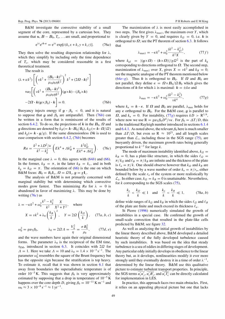
Rep. Prog. Phys. 76 (2013) 096801 P H Roberts and E M King
B&M investigate the convective stability of a smallsegment of the core, represented by a cartesian box. Theyassume that u, B − B0, Tc, . . . are small, and proportional to
eλteık·x = eλt exp[i(kxx + kyy + kzz)]. (76a)
They then solve the resulting dispersion relationship for λ,which they simplify by including only the time dependenceof Tc, which may be considered reasonable in a firsttheoretical treatment.
The result is
(λ + κk2)
[(νk2 +
(B0 · k)2
µ0ρ0ηk2
)2
k2 + (2Ω · k)2
]
+αT
[(νk2 +
(B0 · k)2
µ0ρ0ηk2
)(g×k) · (β0×k)
−2Ω · k(g×β0) · k
]= 0. (76b)
Buoyancy injects energy if g · β0 < 0, and it is naturalto suppose that g and β0 are antiparallel. Then (76b) canbe written in a form that is reminiscent of the results ofsection 6.4.2. To do so, the projections of k in the B0, Ω andg directions are denoted by kB(= k ·B0/B0), kΩ(= k ·Ω/Ω)
and kg(= k · g/g). If the same dimensionless Dk is used toease comparison with section 6.4.2, (76b) becomes
Ra = k2 + λD2/κ
k2 − k2g
(Ek4 + Λk2
B +k2k2
Ω
Ek4 + Λk2B
). (76c)
In the marginal case λ = 0, this agrees with (64b) and (66).In the former, kB = π , in the latter kB = kx , and in bothkg = kΩ = π . The orientation of (66) is the one on whichB&M focus: B0 = B01x , Ω = Ω1z, g = g1z.
The analysis of B&M is not primarily concerned withmarginal stability but with determining which convectivemodes grow fastest. Thus minimizing Ra for λ = 0 isabandoned in favor of maximizing λ. This may be done bywriting (76c) as
λ = −κk2 + ω20
k2 − k2g
k2
X
X2 + Y 2, where
X = νk2 + λ0
(kB
k
)2
, Y = 2Ω
(kΩ
k
), (77a, b, c)
ω20 = gαTβ0, λ0 = 2ΩΛ = V 2
A
η= σB2
0
ρ0, (77d, e)
and the wave numbers have again their original dimensionalforms. The parameter λ0 is the reciprocal of the EM time,τEM, introduced in section 6.3. It coincides with 2Ω forΛ = 1. Here we take Λ = 10 and λ0 = 1.4 × 10⁻³ s−1. Theparameter ω2
0 resembles the square of the Brunt frequency buthas the opposite sign because the stratification is top heavy.To estimate it, recall that it was shown in section 6.1 thataway from boundaries the superadiabatic temperature is oforder 10−5 K. This suggests that β0 is very approximatelyestimated by supposing that a drop in temperature of 10−5 Khappens over the core depth D, giving β0 = 10−11 K m−1 andω0 ≈ 3 × 10⁻⁸ s−1 ≈ 1 yr−1.
The maximization of λ is most easily accomplished intwo steps. The first gives λmax1, the maximum over Y , whichis clearly given by Y = 0, and requires kΩ = 0, i.e. k isorthogonal to Ω; see the PT theorem of section 6.3. It followsthat
λmax1 = −κk2 + ω20
(k2 − k2g1)
k2X, (77f )
where kg1 = |(g×Ω) · (k×Ω)|/gΩ2 is the part of kg
corresponding to directions orthogonal to Ω. The second step,maximization of λmax1 over X, gives X = νk2 and kB = 0;see the magnetic analogue of the PT theorem mentioned below(64e–g). Thus k is orthogonal to B0. If Ω and B0 arenot parallel, they define e = Ω×B0/ΩB0 which gives thedirections of k for which λ is maximal: k = ±ke and
λmax = −κk2 + ω20(k2 − k2
u)
νk4, (77g)
where ku = k · e. If Ω and B0 are parallel, λmax holds forany e orthogonal to B0. For the B&M case, g is parallel toΩ, and ku = 0. For instability, (77g) requires kD > R1/4,where now we use R = gαTβ0D
4/νκ . For β0 = ∆T/D, thisis the traditional Rayleigh number introduced in sections 6.1.4and 6.4.1. As noted above, the relevant β0 here is much smallerthan ∆T/D, but even so R ≈ 1021, and all length scalesgreater than Lν , including those in the SGS range (75), arebuoyantly driven, the maximum growth rates being generallyproportional to k−2 for large k.
The mode of maximum instability identified above, kΩ =kB = 0, has a plate-like structure, in which the sides Ω =π/kΩ and B = π/kB are infinite and the thickness of the plateis u = π/k. One should observe however that kΩ and kB arebounded below by a wave number of order ko = π/ro, eitherdefined by the scale ro of the system or more realistically byLη. In either case, kΩ = kB = 0 is unattainable. Nevertheless,for k corresponding to the SGS scales (75),
ko
k<
kΩ
k 1 and
ko
k<
kB
k 1, (78a, b)
define wide ranges of kΩ and kB in which the sides Ω and Bof the plate are finite and much exceed its thickness u.
St Pierre (1996) numerically simulated the growth ofinstabilities in a special case. He confirmed the growth ofsmall-scale convection that resulted in the plate-like cellspredicted by B&M; see figure 32.
As well as analyzing the initial growth of instabilities bythe linear theory described above, B&M developed a detailedheuristic theory of the fully developed turbulence causedby such instabilities. It was based on the idea that steadyturbulence is a sea of eddies in differing stages of development.Any particular eddy initially develops in obedience to the lineartheory but, as it develops, nonlinearities modify it ever morestrongly until they eventually destroy it in a time of order λ−1,determined by the linear theory. B&M use this qualitativepicture to estimate turbulent transport properties. In principle,the SGS terms u′
iu′j , u′
iB′j , and u′
iT′
c can be directly calculatedfor implementation in LES.
In practice, this approach faces two main obstacles. First,it relies on an appealing physical picture but one that lacks
49
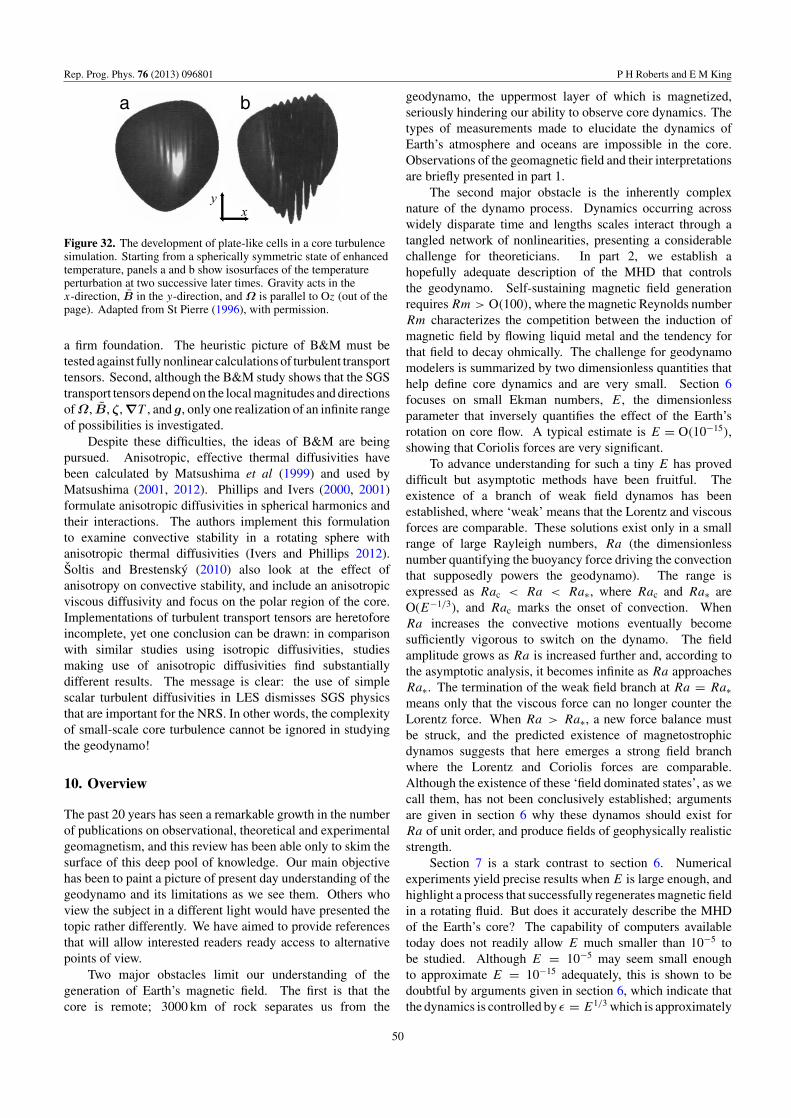
Rep. Prog. Phys. 76 (2013) 096801 P H Roberts and E M King
a b
xy
Figure 32. The development of plate-like cells in a core turbulencesimulation. Starting from a spherically symmetric state of enhancedtemperature, panels a and b show isosurfaces of the temperatureperturbation at two successive later times. Gravity acts in thex-direction, B in the y-direction, and Ω is parallel to Oz (out of thepage). Adapted from St Pierre (1996), with permission.
a firm foundation. The heuristic picture of B&M must betested against fully nonlinear calculations of turbulent transporttensors. Second, although the B&M study shows that the SGStransport tensors depend on the local magnitudes and directionsof Ω, B, ζ, ∇T , and g, only one realization of an infinite rangeof possibilities is investigated.
Despite these difficulties, the ideas of B&M are beingpursued. Anisotropic, effective thermal diffusivities havebeen calculated by Matsushima et al (1999) and used byMatsushima (2001, 2012). Phillips and Ivers (2000, 2001)formulate anisotropic diffusivities in spherical harmonics andtheir interactions. The authors implement this formulationto examine convective stability in a rotating sphere withanisotropic thermal diffusivities (Ivers and Phillips 2012).Soltis and Brestensky (2010) also look at the effect ofanisotropy on convective stability, and include an anisotropicviscous diffusivity and focus on the polar region of the core.Implementations of turbulent transport tensors are heretoforeincomplete, yet one conclusion can be drawn: in comparisonwith similar studies using isotropic diffusivities, studiesmaking use of anisotropic diffusivities find substantiallydifferent results. The message is clear: the use of simplescalar turbulent diffusivities in LES dismisses SGS physicsthat are important for the NRS. In other words, the complexityof small-scale core turbulence cannot be ignored in studyingthe geodynamo!
10. Overview
The past 20 years has seen a remarkable growth in the numberof publications on observational, theoretical and experimentalgeomagnetism, and this review has been able only to skim thesurface of this deep pool of knowledge. Our main objectivehas been to paint a picture of present day understanding of thegeodynamo and its limitations as we see them. Others whoview the subject in a different light would have presented thetopic rather differently. We have aimed to provide referencesthat will allow interested readers ready access to alternativepoints of view.
Two major obstacles limit our understanding of thegeneration of Earth’s magnetic field. The first is that thecore is remote; 3000 km of rock separates us from the
geodynamo, the uppermost layer of which is magnetized,seriously hindering our ability to observe core dynamics. Thetypes of measurements made to elucidate the dynamics ofEarth’s atmosphere and oceans are impossible in the core.Observations of the geomagnetic field and their interpretationsare briefly presented in part 1.
The second major obstacle is the inherently complexnature of the dynamo process. Dynamics occurring acrosswidely disparate time and lengths scales interact through atangled network of nonlinearities, presenting a considerablechallenge for theoreticians. In part 2, we establish ahopefully adequate description of the MHD that controlsthe geodynamo. Self-sustaining magnetic field generationrequires Rm > O(100), where the magnetic Reynolds numberRm characterizes the competition between the induction ofmagnetic field by flowing liquid metal and the tendency forthat field to decay ohmically. The challenge for geodynamomodelers is summarized by two dimensionless quantities thathelp define core dynamics and are very small. Section 6focuses on small Ekman numbers, E, the dimensionlessparameter that inversely quantifies the effect of the Earth’srotation on core flow. A typical estimate is E = O(10−15),showing that Coriolis forces are very significant.
To advance understanding for such a tiny E has proveddifficult but asymptotic methods have been fruitful. Theexistence of a branch of weak field dynamos has beenestablished, where ‘weak’ means that the Lorentz and viscousforces are comparable. These solutions exist only in a smallrange of large Rayleigh numbers, Ra (the dimensionlessnumber quantifying the buoyancy force driving the convectionthat supposedly powers the geodynamo). The range isexpressed as Rac < Ra < Ra∗, where Rac and Ra∗ areO(E−1/3), and Rac marks the onset of convection. WhenRa increases the convective motions eventually becomesufficiently vigorous to switch on the dynamo. The fieldamplitude grows as Ra is increased further and, according tothe asymptotic analysis, it becomes infinite as Ra approachesRa∗. The termination of the weak field branch at Ra = Ra∗means only that the viscous force can no longer counter theLorentz force. When Ra > Ra∗, a new force balance mustbe struck, and the predicted existence of magnetostrophicdynamos suggests that here emerges a strong field branchwhere the Lorentz and Coriolis forces are comparable.Although the existence of these ‘field dominated states’, as wecall them, has not been conclusively established; argumentsare given in section 6 why these dynamos should exist forRa of unit order, and produce fields of geophysically realisticstrength.
Section 7 is a stark contrast to section 6. Numericalexperiments yield precise results when E is large enough, andhighlight a process that successfully regenerates magnetic fieldin a rotating fluid. But does it accurately describe the MHDof the Earth’s core? The capability of computers availabletoday does not readily allow E much smaller than 10−5 tobe studied. Although E = 10−5 may seem small enoughto approximate E = 10−15 adequately, this is shown to bedoubtful by arguments given in section 6, which indicate thatthe dynamics is controlled by ε = E1/3 which is approximately
50

Rep. Prog. Phys. 76 (2013) 096801 P H Roberts and E M King
10−5 in the core but usually exceeds 0.01 in simulations.Moreover, the magnetic Prandtl number, Pm = ν/η, is about10−6 for the liquid metal of the core but in simulations isseldom less than 0.1. The dynamo process that succeeds inthe simulations fails if Pm = 10−6.
Small values of Pm are readily accessible in thelaboratory, and successful experiments are reviewed insection 8, where the difficulties and successes of thisdemanding activity are described. Three of the models usingliquid sodium successfully regenerate magnetic fields. Noneof them, however, are strongly affected by Coriolis forces,and, by practical necessity, are not driven by buoyant forcing,which stifles direct comparison with the geodynamo. Thatraises serious concerns that are addressed but not resolved insection 9.
It is hoped that readers will recognize from this reviewthat the origin of the magnetic field of the Earth is afascinating problem in classical physics which is far frombeing satisfactorily solved. The basics are well understood buttheir development is seriously incomplete. They pose excitingchallenges for the future.
Acknowledgments
We are grateful to Jon Aurnou, Bruce Buffett, Andy Jackson,Masaru Kono and Steve Tobias for gainful discussions onvarious topics within this review. Our thanks are also due tothe following for providing information about their work: UliChristensen, Dominique Jault, Chris Jones, Dan Lathrop, PeterOlson, Krista Soderlund, Andrew Soward and Frank Stefani.Helpful advice from the referees is gratefully acknowledged.
References
Ahlers G, Grossman S and Lohse D 2009 Heat transfer and largescale dynamics in turbulent Rayleigh–Benard convectionRev. Mod. Phys. 81 503–37
Alfven H 1950 Discussion of the origin of the solar and terrestrialmagnetic fields Tellus 2 74–82
Amit H and Christensen U R 2008 Accounting for magneticdiffusion in core flow inversions from geomagnetic secularvariation Geophys. J. Int. 175 913–24
Amit H, Leonhardt R and Wicht J 2010 Polarity reversals frompaleomagnetic observations and numerical dynamo simulationsSpace Sci. Rev. 155 293–335
Aubert J, Amit H, Hulot G and Olson P L 2008 Thermochemicalflows couple the Earth’s inner core growth to mantleheterogeneity Nature 454 758–61
Aubert J, Brito D, Nataf H-C, Cardin P and Masson J-P 2001 Asystematic experimental study of rapidly rotating sphericalconvection in water and liquid gallium Phys. EarthPlanet. Inter. 128 51–74
Aurnou J M, Andreadis S, Zhu L and Olson P L 2003 Experimentson convection in Earth’s core tangent cylinder Earth Planet.Sci. Lett. 212 119–34
Aurnou J M and Aubert J 2011 End-member models ofboundary-modulated convective dynamos Phys. Earth Planet.Inter. 187 353–63
Backus G E 1958 A class of self-sustaining dissipative sphericaldynamos Ann. Phys. N.Y. 4 372–447
Backus G E 1968 Kinematics of geomagnetic secular variation in aperfectly conducting core Phil. Trans. R. Soc. Lond. A263 239–66
Backus G E 1975 Gross thermodynamics of heat engines in the deepinterior of the Earth Proc. Natl Acad. Sci. Wash.72 1555–8
Backus G E 1983 Application of mantle filter theory to the magneticjerk of 1969 Geophys. J. R. Astron. Soc. 74 713–46
Backus G, Parker R and Constable C 1996 Foundations ofGeomagnetism (Cambridge: Cambridge University Press)
Braginsky S I 1963 Structure of the F layer and reasons forconvection in the Earth’s core Sov. Phys.—Dokl 149 8–11
Braginsky S I 1964 Magnetohydrodynamics of the Earth’s coreGeomagn. Aeron. 4 698–712
Braginsky S I 1965a Self-excitation of a magnetic field during themotion of a highly conducting fluid Sov. Phys.—JETP20 726–35
Braginsky S I 1965b Theory of the hydromagnetic dynamo Sov.Phys.—JETP 20 1462–71
Braginsky S I 1967 Magnetic waves in the Earth’s core Geomagn.Aeron. 7 1–97
Braginsky S I 1970 Torsional magnetohydrodynamic vibrations inthe Earth’s core and variations in day length Geomagn. Aeron.10 1–8
Braginsky S I and Meytlis V P 1990 Local turbulence in the Earth’score Geophys. Astrophys. Fluid Dyn. 55 71–87
Braginsky S I and Roberts P H 1995 Equations governingconvection in the Earth’s core and the geodynamo Geophys.Astrophys. Fluid Dyn. 79 1–97
Braginsky S I and Roberts P H 2003 On the theory of convection inthe Earth’s core Advances in Nonlinear Dynamosed A Ferriz-Mas and M Nunez (London: Taylor and Francis)pp 60–82
Braginsky S I and Roberts P H 2007 Anelastic and Boussinesqapproximations Encyclopedia of Geomagnetism andPaleomagnetism ed D Gubbins and E Herrero-Bervera(Heidelberg: Springer) pp 11–9
Brandenburg A, Moss D and Soward A M 1998 New results for theHerzenberg dynamo: Steady and oscillatory solutions Proc. R.Soc. Lond. A 454 1283–300 (erratum, p 3275)
Buffett B A 2003 A comparison of subgrid-scale models forlarge-eddy simulations of convection in the Earth’s coreGeophys. J. Internat. 153 753–65
Buffett B A 2010 Tidal dissipation and the strength of the Earth’sinternal magnetic field Nature 468 952–5
Buffett B A and Bloxham J 2002 Energetics of numericalgeodynamo models Geophys. J. Int. 149 211–24
Buffett B A and Christensen U R 2007 Magnetic and viscouscoupling at the core–mantle boundary; inferences fromobservations of the Earth’s nutations Geophys. J. Int.171 145–52
Buffett B A and Glatzmaier G A 2000 Gravitational braking ofinner-core rotation in geodynamo simulations Geophys. Res.Lett. 27 3125–8
Bullard E C 1949 The magnetic field within the Earth Proc. R.Soc. Lond. A 197 433–53
Bullard E C and Gellman H 1954 Homogeneous dynamos andterrestrial magnetism Phil. Trans. R. Soc. Lond. A247 213–55
Bullard E C and Gubbins D 1977 Generation of magnetic fields byfluid motions of global scale Geophys. Astrophys. Fluid Dyn.8 41–56
Busse F H 1970 Thermal instabilities in rapidly rotating systemsJ. Fluid Mech. 44 441–60
Busse F H 2000 Homogeneous dynamos in planetary cores and inthe laboratory Annu. Rev. Fluid Mech. 32 383–408
Busse F and Carrigan C 1976 Laboratory simulation of thermalconvection in rotating planets and stars Science191 81–3
Busse F and Simitev R D 2006 Parameter dependences ofconvection-driven dynamos in rotating spherical fluid shellsGeophys. Astrophys. Fluid Dyn. 100 341–61
51

Rep. Prog. Phys. 76 (2013) 096801 P H Roberts and E M King
Calkins M A, Aurnou J M, Eldredge J D and Julien K 2012 Theinfluence of fluid properties on the morphology of coreturbulence and the geomagnetic field Earth Planet. Sci. Lett.359–60 55–60
Cardin P and Olson P L 1994 Chaotic thermal convection in arapidly rotating spherical shell: consequences or flow in theouter core Phys. Earth Planet. Inter. 82 235–59
Carrigan C and Busse F 1983 An experimental and theoreticalinvestigation of the onset of convection in rotating sphericalshells J. Fluid Mech. 126 287–305
Chandrasekhar S 1953 The instability of a layer of fluid heatedbelow and subject to Coriolis forces Proc. R. Soc. Lond. A217 306–27
Chandrasekhar S 1954 The instability of a layer of fluid heatedbelow and subject to the simultaneous action of a magneticfield and rotation Proc. R. Soc. Lond. A 225 173–84
Chandrasekhar S 1961 Hydrodynamic and Hydromagnetic Stability(Oxford: Oxford University Press) (Reprinted by Doverpublications)
Chapman S and Bartels J 1940 Geomagnetism II (Oxford:Clarendon) chapter XXVI
Childress S and Gilbert A D 1995 Stretch, Twist, Fold. The FastDynamo (Heidelberg: Springer)
Childress S and Soward A M 1972 Convection-drivenhydromagnetic dynamo Phys. Rev. Lett. 29 837–9
Christensen U R 2010 Dynamo scaling laws and applications to theplanets Space Sci. Rev. 152 565–90
Christensen U R and Aubert J 2006 Scaling properties ofconvection-driven dynamos in rotating spherical shellsGeophys. J. Int. 166 97–114
Christensen U R, Olson P L and Glatzmaier G A 1999 Numericalmodelling of the geodynamo: a systematic parameter studyGeophys. J. Int. 138 393–409
Christensen U R and Tilgner A 2004 Power requirement of thegeodynamo from ohmic losses in numerical and laboratorydynamos Nature 429 169–171
Christensen U and Wicht J 2007 Numerical dynamo simulationsTreatise on Geophysics vol 8 ed P Olson (Amsterdam:Elsevier) pp 207–43
Clement B M 2004 Dependence of the duration of geomagneticpolarity reversals on site latitude Nature 428 637–40
Courtillot V and LeMouel J-L 1984 Geomagnetic secular variationimpulses Nature 311 709–16
Cowling T G 1933 The magnetic field of sunspots Mon. Not. R.Astron. Soc. 94 39–48
Davies C J, Gubbins D and Jimack P K 2009 Convection in arapidly rotating spherical shell with an imposed laterallyvarying thermal boundary condition J. Fluid Mech.641 335–58
Davies C J, Gubbins D and Jimack P K 2011 Scalability ofpseudospectral methods for geodynamo simulationsConc. Computat.: Pract. Exper. 23 38–56
Deguen R 2012 Structure and dynamics of Earth’s inner core EarthPlanet. Sci. Lett. 333–334 211–25
Dormy E 1997 Modelisation num^rique de la dynamo terrestre.PhD Thesis Institut de Physique du Globe de Paris
Dormy E, Soward A M, Jones C A, Jault D and Cardin P 2004 Theonset of thermal convection in rotating spherical shells J. FluidMech. 501 43–70
Dudley M L and James R W 1989 Time-dependent kinematicdynamos with stationary flows Proc. R. Soc. Lond. A425 407–29
Dziewonski A M and Anderson D L 1981 Preliminary referenceEarth model Phys. Earth Planet. Inter. 25 297–356
Elphic R C and Russell C T 1978 On the apparent sourcedepth of planetary magnetic fields Geophys. Res. Lett.5 211–4
Elsasser W 1946 Induction effects in terrestrial magnetism: II. Thesecular variation Phys. Rev. 70 202–12
Elsasser W M 1947 Induction effects in terrestrial magnetism:III. Electric modes Phys. Rev. 72 821–33
Eltayeb I A 1972 Hydromagnetic convection in a rapidly rotatingfluid layer Proc. R. Soc. Lond. A 326 229–54
Eltayeb I A and Roberts P H On the hydromagnetics of rotatingfluids Astrophys. J. 162 699–701
Fautrelle Y and Childress S 1982 Convective dynamos withintermediate and strong fields Geophys. Astrophys. Fluid Dyn.22 235–79
Fearn D R 1998 Hydromagnetic flow in planetary coresRep. Prog. Phys. 61 175–235
Finlay C C and Amit H 2011 On flow magnitude and field-flowalignment at Earth’s core surface Geophys. J. Int.186 175–92
Finlay C, Dumberry M, Chulliat A and Pais M A 2010a Shorttimescale core dynamics: theory and observations Space Sci.Rev. 155 177–218
Finlay C C et al 2010b International geomagnetic reference field:the eleventh generation Geophys. J. Int. 183 1216–30
Gailitis A et al 2000 Detection of a flow induced magnetic fieldeigenmode in the Riga dynamo facility Phys. Rev. Lett.84 4365–8
Gailitis A, Lielausis S, Platacis A, Gerbeth G and Stefani F 2002Laboratory experiments on hydromagnetic dynamosRev. Mod. Phys. 74 973–90
Gailitis A, Lielausis O, Platacis E, Gerbeth G and Stefani F 2003The Riga dynamo experiment Surv. Geophys.24 247–67
Giesecke A, Stefani F and Gerbeth G 2010 Role of soft-ironimpellers on the mode selection in the von Karman–sodiumdynamo experiment Phys. Rev. Lett. 104 044503
Gillet N, Brito D, Jault D and Nataf H-C 2007 Experimental andnumerical studies of convection in a rapidly rotating sphericalshell J. Fluid Mech. 580 83–121
Gillet N, Jault D, Canet E and Fournier A 2010 Fast torsional wavesand strong magnetic field within the Earth’s core Nature465 74–7
Gissinger C, Iskakov A, Fauve S and Dormy E 2008 Effect ofmagnetic boundary conditions on the dynamo threshold ofvon Karman swirling flows Europhys. Lett. 82 29001
Glatzmaier G A 1984 Numerical simulations of stellar convectivedynamos: I. The model and method J. Comput. Phys.55 461–84
Glatzmaier G A, Coe R S, Hongre L and Roberts P H 1999 The roleof the Earth’s mantle in controlling the frequency ofgeomagnetic reversals Nature 401 885–90
Glatzmaier G A and Roberts P H 1995a A three–dimensionalconvective dynamo solution with rotating and finitelyconducting inner core and mantle Phys. Earth Planet. Inter.91 63–75
Glatzmaier G A and Roberts P H 1995b A three-dimensionalself-consistent computer simulation of a geomagnetic fieldreversal Nature 377 203–9
Glatzmaier G A and Roberts P H 1996a Rotation and magnetism ofthe Earth’s inner core Science 274 1887–92
Glatzmaier G A and Roberts P H 1996b On the magnetic soundingof planetary interiors Phys. Earth Planet. Inter. 98 207–20
Glen W 1982 The Road to Jaramillo (Stanford CA: StanfordUniversity Press)
Gubbins D 2001 The Rayleigh number for convection in the Earth’score Phys. Earth Planet. Inter. 128 3–12
Gubbins D and Herrero-Bervera E (ed) 2007 Encyclopedia ofGeomagnetism and Paleomagnetism (Heidelberg: Springer)
Herzenberg A 1958 Geomagnetic dynamos Phil. Trans. R. Soc.Lond. A 250 543–83
Hewitt J M, McKenzie D P and Weiss N O 1975 Dissipative heatingin convective flows J. Fluid Mech. 68 721–38
Hide R 1974 Jupiter and Saturn, Proc. R. Soc. Lond. A336 63–84
52

Rep. Prog. Phys. 76 (2013) 096801 P H Roberts and E M King
Hide R 1978 How to locate the electrically conducting fluid core of aplanet from external magnetic observations Nature 271 640–1
Holme R and Olsen N 2006 Core surface flow modelling fromhigh-resolution secular variation Geophys. J. Int. 166 518–28
Hulot G, Lhuillier F and Aubert J 2010 Earth’s dynamo limit ofpredictability Geophys. Res. Lett. 37 L06305
Iida T and Guthrie R I L 1993 The Physical Properties of LiquidMetals (Oxford: Oxford Clarendon Press)
Ivers D J and James R W 1984 Axisymmetric antidynamo theoremsin non-uniform compressible fluids Phil. Trans. R.Soc. Lond. A 312 179–218
Ivers D J and Phillips C G 2012 Anisotropic turbulent thermaldiffusion and thermal convection in a rapidly rotating fluidsphere Phys. Earth Planet. Inter. 190–1 1–9
Jackson A, Jonkers A R T and Walker M R 2000 Four centuries ofgeomagnetic data from historical records Phil. Trans. R.Soc. Lond. A 358 957–90
Jacobs J A 1953 The Earth’s inner core Nature 172 297–98Johnson C and Constable C 1997 The time-averaged geomagnetic
field: global and regional biases for 0–5 Ma Geophys. J. Int.131 643–66
Johnson C et al 2008 Recent investigations of the 0–5 Mageomagnetic field recorded by lava flowsGeochem. Geophys. Geosyst. 9 Q04032
Jones C A 2011 Planetary magnetic fields and fluid dynamosAnnu. Rev. Fluid Mech. 43 583–614
Jones C A, Moore D R and Weiss N O 1976 Axisymmetricconvection in a cylinder J. Fluid Mech. 73 353–88
Jones C A, Soward A M and Mussa A I 2000 The onset of thermalconvection in a rapidly rotating sphere J. Fluid Mech.405 157–79
Kageyama A, Miyagoshi T and Sato T 2008 Formation of currentcoils in geodynamo simulations Nature 454 1106–9
Kageyama A and Sato T 1997, Generation mechanism of a dipolefield by a magnetohydrodynamic dynamo Phys. Rev. E55 4617–26
Kelley D, Triana S, Zimmerman D, Tilgner A and Lathrop D 2007Inertial waves driven by differential rotation in a planetarygeometry Geophys. Astrophys. Fluid Dyn.101 469–87
Kennett B L N, Engdahl E R and Buland R 1995 Constraints onseismic velocities in the Earth from travel times Geophys. J.Int. 122 108–24
Kent D V and Gradstein F M A 1986 Jurassic to recent chronology.The Geology of North America vol M ed P R Vogt andB E Tucholke (Boulder, CO: Geological Society of America)pp 45–50
Kerswell R R 1996 Upper bounds on the energy dissipation inturbulent precession J. Fluid Mech. 321 335–70
King E M and Aurnou J M 2013 Turbulent convection in liquidmetal with and rotation Proc. Natl Acad. Sci. 110 6688–93
King E M and Buffett B A 2013 Flow speeds and length scales ingeodynamo models: the role of viscosity Earth Planet. Sci.Lett. 371 156–62
King E M, Soderlund K M, Christensen U R, Wicht J andAurnou J M 2010 Convective heat transfer in planetary dynamomodels Geochem. Geophys. Geosyst. 11 1–19
King E M, Stellmach S, Noir J, Hansen U and Aurnou J M 2009Boundary layer control of rotating convection systems Nature457 301–4
Kono M (ed) 2006 Geomagnetism (Amsterdam: Elsevier)Kono M and Tanaka H 1995 Intensity of the geomagnetic field in
geological time. A statistical study The Earth’s central Part. ItsStructure and Dynamics ed T Yukutake (Tokyo: TerraPub)pp 75–94
Krause F and Radler K-H 1980 Mean-Field Electrodynamics andDynamo Theory (Berlin: Academic)
Kuang W and Bloxham J 1997 An Earth-like numerical dynamomodel Nature 389 371–4
Kuang W, Jiang W and Wang T 2008 Sudden termination of Martiandynamo: implictions from subcritical dynamo simulationsGeophys. Res. Lett. 35 L14204
Kutzner C and Christensen U R 2002 From stable dipolar towardsreversing numerical dynamos Phys. Earth Planet. Inter.131 29–45
Labrosse S 2003 Thermal and magnetic evolution of the Earth’s corePhys. Earth Planet. Inter. 140 127–43
Laguerre R, Nore C, Ribeiro A, Leorat J, Guermond J-L andPlunian F 2008 Impact of impellers on the axisymmetricmagnetic mode in the VKS2 dynamo experiment Phys. Rev.Lett. 101 104501
Landau L D and Lifshitz E M 1987 Fluid Mechanics 2nd edn(Oxford: Pergamon)
Langel R A 1987 The main geomagnetic field Geomagnetism vol 1ed J A Jacobs (San Diego, CA: Academic) pp 249–512
Lanzerotti L J, Sayres C H, Medford L V, Kraus J S andMaclennan C G 1992 Earth potential over 4000 km betweenHawaii and California Geophys. Res. Lett. 19 1177–80(Correction p 1321, (doi:10.1029/92GL01328))
Loper D E 1978 The gravitationally powered dynamo Geophys. J. R.Astron. Soc. 54 389–404
Loper D E 1984 Structure of the core and lower mantleAdv. Geophys. 26 1–34
Lowes F J 1966 Mean square values on the sphere of sphericalharmonic vector fields J. Geophys. Res. 71 2179
Lowes F J 1974 Spatial power spectrum of the main geomagneticfield and extrapolation to the core Geophys. J. R. Astron. Soc.36 717–30
Lowes F J and Wilkinson I 1963 Geomagnetic dynamo: a laboratorymodel Nature 198 1158–60
Lowes F J and Wilkinson I 1968 Geomagnetic dynamo: animproved laboratory model Nature 219 717–8
Mandea M, Holme R, Pais A, Pintheiro K, Jackson A, Verbanac G2010 Geomagnetic jerks; rapid core field variations and coredynamics Space Sci. Rev. 155 147–75
Matsui H and Buffett B A 2012 Large-eddy simulations ofconvection-driven dynamos using a dynamic scale-similaritymodel Geophys. Astrophys. Fluid Dyn. 106 250–76
Matsushima M 2001 Expression of turbulent heat flux in the Earth’score in terms of a second moment closure model Phys. EarthPlanet. Inter. 128 137–48
Matsushima M 2012 The effect of anisotropic diffusivity on rotatingmagnetoconvection in the Earth’s core Geophys. Astrophys.Fluid Dyn. 106 630–42
Matsushima M, Nakajima T and Roberts P H 1999 The anisotropyof local turbulence in the Earth’s core Earth Planets Space51 277–86
Mauersberger P 1956 Das Mittel der energiedichte desgeomagnetischen Hauptfeldes an der erdoberflasche und seinesakulare Anderung. Gerlands Beitr. Geophys. 65 207–15
Merrill R T, McElhinny M W and McFadden P L 1996 TheMagnetic Field of the Earth. Paleomagnetism, the Core and thedeep Mantle (San Diego, CA: Academic)
Miyagoshi T, Kageyama A and Sato T 2011 Formation of sheetplumes, current coils, and helical magnetic fields in aspherical magnetohydrodynamic dynamo Phys. Plasmas18 072901
Moffatt H K 1969 The degree of knottiness of tangled vortex linesJ. Fluid Mech. 35 117–29
Moffatt H K 1978 Magnetic Field Generation in electricallyconducting Fluids (Cambridge: Cambridge University press)
Monchaux R et al 2007 Generation of a magnetic field by dynamoaction in a turbulent flow of liquid sodium Phys. Rev. Lett.98 044502
Monchaux R et al 2009 The von Karman Sodium experiment:turbulent dynamical dynamos Phys. Fluids 21 035108
Moreau J J 1961 Constants d’un ılot tourbillonnaire en fluide parfaitbarotrope C. R. Acad. Sci. Paris 252 2810–2
53
Rep. Prog. Phys. 76 (2013) 096801 P H Roberts and E M King
Muller U, Stieglitz R and Horanyi S 2006 Experiments at atwo-scale dynamo test facility J. Fluid Mech. 552 419–40
Nakagawa Y 1957 Experiments on the instability of a layer ofmercury heated from below and subject to the simultaneousaction of a magnetic field and rotation Proc. R. Soc. Lond. A242 81–8
Olsen N and Mandea M 2008 Rapidly changing flows in the Earth’score Nature Geosci. 1 390–4
Olson P L and Aurnou J M 1999 A polar vortex in the Earth’s coreNature 402 170–3
Olson P L, Christensen U R and Glatzmaier G A 1999 Numericalmodeling of the geodynamo: Mechanisms of field generationand equilibration J. Geophys. Res. 104 10383–404
Parker E N 1955 Hydromagnetic dynamo models Astrophys. J.122 293–314
Petrelis F, Besse J and Valet J P 2011 Plate tectonics may controlgeomagnetic reversal frequency Geophys. Res. Lett. 38 L1–4
Petrelis F and Fauve 2008 Chaotic dynamics of the magnetic fieldgenerated by dynamo action in a turbulent flow J. Phys.Condens. Matter. 20 494203
Petrelis F, Fauve S and Valet J-P 2009 Simple mechanism forreversals of Earth’s magnetic field Phys. Rev. Lett.102 144503
Phillips C G and Ivers D J 2000 Spherical anisotropic diffusionmodels for the Earth’s core Phys. Earth Planet. Inter.117 209–23
Phillips C G and Ivers D J 2001 Spectral interactions ofrapidly-rotating anisotropic turbulent viscous and thermaldiffusion in the Earth’s core Phys. Earth Planet. Inter.128 93–107
Pollack H N, Hurter S J and Johnson J R 1993 Heat flow from theEarth’s interior: analysis of the global data set Rev. Geophys.31 267–80
Ponomarenko Yu 1973 On the theory of the hydromagnetic dynamoJ. Appl. Mech. Tech. Phys. 14 775–8
Pozzo M, Davies C, Gubbins D and Alfe D 2012 Thermal andelectrical conductivity of iron at Earth’s core conditions Nature485 355–8
Proudman J 1916 On the motion of solids in liquids possessingvorticity Proc. R. Soc. Lond. A 92 408–24
Ravelet F et al 2008 Chaotic dynamos generated by a turbulent flowof liquid sodium Phys. Rev. Lett. 101 074502
Reuter K, Jenko F and Forest C B 2011 Turbulentmagnetohydrodynamic dynamo action in a spherically boundedvon Karman flow at small magnetic Prandtl numbers New J.Phys. 13 073019
Roberts G O 1972 Dynamo action of fluid motions withtwo-dimensional periodicity Phil. Trans. R. Soc. Lond. A271 411–54
Roberts P H 1968 On the thermal instability of a rotating-fluidsphere containing heat sources Phil. Trans. R. Soc. Lond. A263 93–117
Roberts P H 1971 Dynamo theory Mathematical Problems in theGeophysical Sciences: Inverse Problems, Dynamo Theory andTides ed W H Reid (Providence RI: American MathematicalSociety) pp 129–206
Roberts P H 2007 Theory of the geodynamo Core Dynamicsed P Olson (Amsterdam: Elsevier) pp 67–105
Roberts P H 1993 Dynamo theory Astrophysical Fluid Dynamicsed J P Zahn and J Zinn-Justin (Amsterdam: Elsevier)pp 229–323
Roberts P H and Aurnou J M 2012 On the theory ofcore–mantle coupling Geophys. Astrophys. Fluid Dyn.106 157–230
Roberts P H and Gubbins D 1987 Origin of the main field:Kinematics Geomagnetism vol 2 ed J A Jacobs (San Diego,CA: Academic) pp 185–249
Roberts P H and Lowes F J 1961 Earth currents of deep internalorigin J. Geophys. Res. 66 1243–54
Sakuraba A and Roberts P H 2009 Generation of a strong magneticfield using uniform heat flux at the surface of the core NatureGeosci. 2 802–5
Saltzman B (ed) 1962 Selected Papers on the Theory of ThermalConvection with Special Application to the Earth’s PlanetaryAtmosphere (New York: Dover)
Schekochihin A A, Haugen N E L, Brandenburg A, Cowley S C,Maron J L and McWilliams J C 2005 The onset of asmall-scale turbulent dynamo at low magnetic Prandtl numbersAstrophys. J. 625 115–8
Schubert G, Turcotte D L and Olson P 2001 Mantle Convection inthe Earth and Planets (Cambridge: Cambridge UniversityPress)
Shimizu H and Utada H 2004 The feasibility of using decadalchanges in the geoelectric field to probe Earth’s corePhys. Earth Planet. Inter. 142 297–319
Shimizu H, Koyama T and Utada H 1998 An observationalconstraint on the strength of the toroidal magnetic field at theCMB by time variation of submarine cable voltagesGeophys. Res. Lett. 25 4023–6
Soderlund K M, King E M and Aurnou J M 2012 The weakinfluence of magnetic fields in planetary dynamo models EarthPlanet. Sci. Lett. 333–334 9–20
Soltis T and Brestensky J 2010 Rotating magnetoconvection withanisotropic diffusivities in the Earth’s core Phys. Earth Planet.Inter. 178 27–38
Song X and Richards P G 1996 Seismological evidence fordifferential rotation of Earth’s inner core Nature 382 221–4
Souriau A 2007 Deep earth structure—The Earth’s core. Seismologyand Structure of the Earth Treatise on Geophysics vol 1ed B A Romanowicz and A M Dziewonski (Amsterdam:Elsevier) pp 655–93
Soward A M 1972 A kinematic theory of large magnetic Reynoldsnumber dynamos Phil. Trans. R. Soc. Lond. A 272 431–62
Soward A M 1974 A convection-driven dynamo 1. Weak-field casePhil. Trans. R. Soc. Lond. A 275 611–46
Soward A M and Roberts P H 2014 Eulerian and Lagrangian meansin rotating, magnetohydrodynamic Flows II. Braginsky’snearly axisymmetric dynamo Geophys. Astrophys. Fluid Dyn.in review
Spence E, Nornberg M, Jacobson C M, Kendrick R and Forest C B2006 Observation of a turbulence-induced large scale magneticfield Phys. Rev. Lett. 96 055002
Sreenivasan B and Jones C A 2006 The role of inertia inthe evolution of spherical dynamos Geophys. J. Int.164 467–76
Sreenivasan B and Jones C A 2011 Helicity generation andsubcritical behaviour in rapidly rotating dynamos J. FluidMech. 688 5–30
St Pierre M G 1996 On the local nature of turbulence inEarth’s outer core Geophys. Astrophys. Fluid Dyn.83 293–306
Stacey F 1992 Physics of the Earth 3rd edn (Brisbane, Australia:Brookfield Press)
Stacey F D and Irvine R D 1977 Theory of melting: thermodynamicbasis of Lindemann’s law Aus. J. Phys. 30 631–40
Starchenko S and Jones C A 2002 Typical velocities and magneticfield strengths in planetary interiors Icarus 157 426–35
Steenbeck M, Krause F and Radler K-H 1966 Berechnung dermittleren Lorentz–Feldstarke u × B fur ein elektrischleitendendes Medium in turbulenter, durch Coriolis–Kraftebeeinflußter Bewegung Z. Naturf. a 21 369–76
Stellmach S and Hansen U 2004 Cartesian convection drivendynamos at low Ekman number Phys. Rev. E 70 1–16
Stieglitz R and Muller U 2001 Experimental demonstration of ahomogeneous two-scale dynamo Phys. Fluids 13 561–4
Sumita I and Olson P L 2000 Laboratory experiments on highRayleigh number thermal convection in a rapidly rotatinghemispherical shell Phys. Earth Planet. Inter. 117 153–70
54

Rep. Prog. Phys. 76 (2013) 096801 P H Roberts and E M King
Takahashi F, Matsushima M and Honkura Y 2008 Scale variabilityin convection-driven MHD dynamos at low Ekman numberPhys. Earth Planet. Inter. 167 168–78
Takahashi F and Shimizu H 2012 A detailed analysis of a dynamomechanism in a rapidly rotating spherical shell J. Fluid Mech.701 228–50
Taylor J B 1963 The magnetohydrodynamics of a rotating fluid andthe Earth’s dynamo problem Proc. R. Soc. Lond. A 274 274–83
Taylor G I 1918 Motion of solids in fluids when the flow is notirrotational Proc. R. Soc. Lond. A 93 99–113
Taylor G I 1921 Experiments with rotating fluids Proc. R.Soc. Lond. A 100 114–21
Tkalcic H, Young M, Bodin T, Ngo S and Sambridge M 2013 Theshuffling rotation of the Earth’s inner core revealed byearthquake doublets Nature Geosci. 6 497–504
Tobias S M, Cattaneo F and Boldyrev S 2013 MHD dynamos andturbulence Ten Chapters in Turbulence ed P Davidson et al(Cambridge: Cambridge University Press)
Turcotte D L and Oxburgh E R 1967 Finite amplitude convectivecells and continental drift J. Fluid Mech. 28 29–42
Valet J-P, Fournier A, Courtillot V and Herrero-Bervera E 2012Dynamical similarity of geomagnetic field reversals Nature490 89–93
Weiss N O 1966 The expulsion of magnetic flux by eddies Proc. R.Soc. Lond. A 293 310–28
Wicht J and Christensen U R 2010 Torsional oscillations in dynamosimulations Geophys. J. Int. 181 1367–80
Wicht J, Stellmach S and Harder H 2009 Numerical modelsof the geodynamo: From fundamental Cartesian models to3D simulations of field reversals GeomagneticField Variations ed K H Glaßmaier et al (Berlin: Springer)
Wicht J and Tilgner A 2010 Theory and modeling of planetarydynamos Space Sci. Rev. 152 501–42
Willis A P, Sreenivasan B and Gubbins D 2007 Thermalcore–mantle interaction: exploring regimes for ‘locked’dynamo action Phys. Earth Planet. Inter. 167 83–92
Wu C-C 2007 A high order WENO finite difference scheme forincompressible fluid and magnetohydrodynamicsGeophys. Astrophys. Fluid Dyn. 101 37–61
Zhang K 1995 Spherical shell rotating convection in the presence oftoroidal magnetic field Proc. R. Soc. Lond. A 448 245–68
Zhang K and Jones C A 1996 On small Roberts numbermagnetoconvection in rapidly rotating systems Proc. R.Soc. Lond. A 452 981–95
Zhang K and Schubert G 2000 Magnetohydrodynamics in rapidlyrotating spherical systems Annu. Rev. Fluid Mech. 32 409–43
55