Embed Size (px)
Citation preview
ON T H E F O U N D A T I O N S OFCLASSICAL STATISTICAL
PHYSICS
\ #f \ rp \ l M 'SK ) '2V i \ J p
J. VAN DER LINDEN


Icot-st diS^»erto>-t<-a-S

ON THE FOUNDATIONS OFCLASSICAL STATISTICAL PHYSICS'
if*'* y 'H{ * / iKsnwur-1, ,1 t«WZ / TO

ON T H E F O U N D A T I O N S OFCLASSIC AL STATISTICAL
P H Y S IC SR
PROEFSCHRIFT
T E R V E R K R I J G I N G V A N D E G R A A D V A N D O C T O R I N
D E W I S K U N D E E N N A T U U R W E T E N S C H A P P E N A A N D E
R I J K S U N I V E R S I T E I T T E ' L E I D E N , O P G E Z A G V A N D E
R E C T O R M A G N I F I C U S DR. J. D A N K M E I J E R , H O O G L E R A A R
I N D E F A C U L T E I T D E R G E N E E S K U N D E , T E N O V E R S T A A N
V A N E E N C O M M I S S I E U I T D E S E N A A T T E V E R D E D I G E N
O P W O E N S D A G 26 J A N U A R I 1966 T E 16 U U R
D O O R
JOHANNES VAN DER LINDENG E B O R E N T E V L A A R D I N G E N I N 1935
w
- J i
K O N I N K L I J K E D R U K K E R I J V A N D E G A R D E N.V.
Z A L T B O M M E L
P romotor: P rof. Dr . P. Mazur

The incorporation of thermodynamics within mechanics isa classic and generally familiar instance of a reduction ofdissimilar theories.
E rn est N agel, The Structure of Science

The research described in this thesis has been carried out under the auspices of the “Stichtingvoor Fundamenteel Onderzoek der Materie (F.O.M.)”, financially supported by the NetherlandsOrganisation for the Advancement of Pure Research (Z.W.O.).
CONTENTS
Introduction.......................................................................................................
Chapter 1 — The asymptotic problem of statistical thermodynamics for areal system1. Introduction.................................. 12. Statement of the asymptotic problem.......................................... 23. Proof of the existence of the functions s(m>, ƒ<«*), p is ') ................... 74. Equivalence of the various formalisms.......................................... 125. Remaining q u estio n s ............................................................. ... 186. Discussion ......................................................................................... 24Appendix.....................................................................................................25R eferences............... . ........................................................................ 27
Chapter II - Survey of related topics1. The Legendre transformation in thermodynamics............................282. Statement of the ergodic problem of statistical mechanics . . . 323. The various formalisms of statistical physics . ................................ 374. The limit theorems of probability theory........................................... 415. The asymptotic properties of a separable s y s te m ............................466. Stability of the pair potential..............................................................53Appendix................................................................................................ ......References.................................. 61
Samenvatting ............................................................................................. 62
Studiegegevens.....................................................................................^ 6 3
VII

INTRODUCTION
The branch of theoretical physics investigating the foundations ofstatistical physics, consists of two parts. The first part tries to explainwhy it is permissible to use a statistical phase average of a relevant mechanicalquantity, instead of its time average (the ergodic problem). The second partis interested in the existence and other properties of the so-called thermodynamic limit of the functions of statistical thermodynamics (the asymptoticproblem). A treatment of these problems can be either classical or quantal,but in this thesis only the first possibility comes up for discussion. As amatter of fact, the theory of statistical physics can only be considered tobe founded in a satisfactory way, if the underlying properties of the interaction potential are in agreement with what is known from other fields ofmolecular physics. Since at first this was found to be too hard a task,simplifying potential models were introduced. Until almost half a centuryafter G ibbs’ rather intuitive ensemble theory (1902),the interaction had tobe even altogether neglected (separable system, e.g. the ideal gets) in orderto get any results. This period was closed in a brilliant way by the workof K hinchin.
The asymptotic problem consists of at least three separate existence-of-a-limit questions for each of the three formalisms of statistical thermodynamics (microcanonical, canonical and grand canonical); the mostimportant properties to be established for the limit functions are theequivalence relations (implying that each formalism generates the samethermodynamics). Now for a separable system, the asymptotic problemreduces to the equivalence question, and the method of proof developed byK hinch in is characterized by the application of the central limit theoremof probability theory.
The investigation of real systems was opened by Van H ove’s paper onthe existence of the thermodynamic limit of the canonical free energy (1949).The treatment of this limit and the corresponding one in the grand canonicalformalism (the pressure), has finally been drawn out of the stage of unsatisfactory potential models by F ish e r and Ruelle, independently(1963/64). About the same time Gri f f i ths derived a remarkably simple
theorem with the consequence that actually five instead of two limits wereestablished definitely.
A crucial requirement of the pair potential, found in this recent work,is the “stability” , which means the following. Taking into account only thefact that the pair potential has a finite minimum, the minimum interactionenergy of N particles is seen to satisfy the inequality “E ff > a negativeconstant times N p ” with p = 2. For 1 < p < 2, however, the free energyper particle blows up for N -> oo, whereas for 0 ^ p ^ 1, it may tend toa finite limit. Therefore the potential is called stable if the inequality issatisfied with p = 1. The Lennard-Jones potential, for example, is shownto be stable, and to accomplish actually the existence of the limits mentionedabove.
The object of investigation which has led to this thesis, has been theextension of the asymptotic results for real systems to the equivalencequestion, following up the ideas of K hinch in concerning the use of probability theory. The derivation of the equivalence relations given in chapter I,is based op a potential which is stable and “strongly tempered” (i.e. negativeat large enough distances). The method of proof is a synthesis of elementsdue to K hinch in (application of the central limit theorem) and F isher(use of subadditivity). Moreover the number of functions for which thethermodynamic limit is shown to exist, is increased with two microcanonicalones: the entropy and the temperature.
Since this first chapter is written in the form of a research report (it willappear as such in “Physica”), it is rather compact. Therefore a secondchapter is added which elaborates some points only referred to in chapter I.The following scheme of correspondences should be noted:
Chapter I Chapter II
§ 2. thermodynamicsstatistical functionsergodic problemstability of the interactionGriffiths’ theorem
§ 6. phase transition problem§ 4. Khinchin’s asymptotic results
§ 1 -§3.§ 2, § 5.§ 6.Appendix§4, §5.§ 6, Appendix
Chapter I
ON THE ASYMPTOTIC PROBLEM OF STATISTICALTHERMODYNAMICS FOR A REAL SYSTEM
§ 1. Introduction. Statistical thermodynamics gives a prescription how todetermine “thermodynamic analogies” from a statistical function (canonicalor grand canonical partition function; in the microcanonical case there issome ambiguity). These analogies are supposed to represent asymptoticallythe corresponding thermodynamic functions in the “thermodynamic limit”.The first question we encounter is therefore: (a) does the existence of suchlimits indeed follow from the properties of the interaction entering in thedefinition of the statistical functions? This question may be split into twoparts: (a') for those analogies which are simply proportional to the logarithmof a statistical function (microcanonical entropy, canonical free energy,and grand canonical pressure), (a") for all others. As is well-known, the limitfunctions to which (a') refers, imply the knowledge of all other thermodynamic functions, so that we may ask: (b) whether the latter determinationagrees with the limit functions to which (a") refers. Furthermore, there is theimportant question concerning: (c) the equivalence of the various formalisms,on the basis of the relations between any two of the statistical functions. Allthis together constitutes the asymptotic problem of statistical thermodynamics (for a detailed statement, and a survey of its treatment in sections3-5, see section 2).
At first separable systems (for example the ideal gas) were considered.Then the canonical and grand canonical partition functions factorize, sothat in these formalisms the questions (a) and (b) present no difficulty. Thetreatment of the remaining problem for such systems in general (i.e. withoutreference to the internal structure of the non-interacting components),has been brought into its simplest form b y K h in c h in 1). The feature of hisapproach is that the asymptotic evaluation of a statistical function (structure function or canonical partition function) is conceived as a limit problemof probability theory, to which the so-called central limit theorem is applicable.
1
Then the way was paved for the consideration of nonseparable systemswhere (a) and (b), in the canonical and the grand canonical formalisms, arealso problematic. The treatment of (a') in these cases has had an evolutionof its own: from the consideration of systems with hard core-finite rangeinteraction, to the latest developments on the basis of very general interaction properties (a review of this has been given by R u elle2)). In itsearliest stage the approach to these existence problems has served as a basisfor Y am am oto and M atsu d a3) in extending K hinch in ’s work on theequivalence problem, and in its recent stage it has done so again for us (fora discussion of the various methods involved, including that of our previouspaper4), see section 6).
In dealing with (a") and (b), as well as with (c), we have also takenadvantage of the conditions on the interchangeability of the thermodynamiclimit and differentiation, found recently by G rif f ith s5) (in connectionwith a treatment of the question (a') in the quantum canonical formalismfor a spin system).
§ 2. Statement of the asymptotic problem. In classical statistical thermodynamics one determines from the Hamiltonian function of a system theGibbsian analogies of its thermodynamic functions. For a system of Nidentical point particles with mass m and pair interaction, the Hamiltonianfunction depends on the configuration rN = (iq, ..., rN) and the setof momenta p N = (pi, ..., P n ) as follows,
(■0N) 2 *Jr N{r*, p N) = - V - + E *(|r< - r,\). 0)
2m 1,1=1i<1
where u is the pair potential. All positions rt(i = 1 ,...,N) are restricted tothe volume V of the system.
Besides N and V, we will consider the following thermodynamic quantities: E, the internal energy, S, the entropy divided by k (Boltzmannsconstant), /S, the inverse absolute temperature divided by k, F, the freeenergy multiplied by —/?, /.i, the chemical potential multiplied by ft, andp, the pressure multiplied by /?. Instead of the extensive quantities V, E, Sand F, we will mostly use their specific values v = V /N , e = EfN, s = S/Nand ƒ = F/N. Of the set of seven intensive quantities thus obtained, twoare independently variable. For any choice of them we have
f = s — fie, (2)
H = / — pv. (3)
There are three alternative ways in common use to determine thermodynamic analogies from y, each of which is based on one of the statistical
2
functions En, On and Sy given by
En {E, V) = ~ j j d r N dpNa{E - Jt?N(r», p*)},
(E0{E, V) = a{E)), - o o < E < oo, (4)
where a denotes the unit-step function,
0v(/S, V) = — ƒ ƒ dr-^ dpN exp {— N(rN, pN)},
(Ö>o(/S, V) = 1), 0 < ft < oo, (5)and
OO
f*) = El T), —OO < n < oo. (6)jv-o
According to the microcanonical formalism, the logarithm of the function(4) is the analogy Sffl of S as a function of N, E and V, or written withspecific values,
f v) = -jj- log EN(Ne,Nv)*). (7)
The analogies of the remaining thermodynamic functions are derived fromthis basic one by means of “thermodynamic” formulae:tfe|g§Jg m
(9)
and (2) and (3) applied to this formalism.The connection of this theory with thermodynamics is based on two
suppositions. The first one is: the sequence of functions defined by (7) forN = 0, 1 , 2, 3, . . . attains a finite limit s<m*,
lim s<“ > (e, v) = s<®> (e, v), (10)N -*co
which operation may be interchanged with differentiation so that for (8)and (9)
lim P^\e, v) — v) as (e> v) (i i)jV ->oo 06
lim p(x \ e , v) = p(m)(e, v) = Ss ^ . (12)V —oo ov
*) For our purpose this is the most convenient one of the two alternative microcanonicalentropy analogies; see furthermore section 5.
3
The second supposition is that these limit functions are the true thermodynamic functions. Then s fr \ f t ^ \ etc. are very good approximations formacroscopic systems (N 1023) to s, ft, etc. as functions of e and v. If wedo not use specific quantities, we say that S f f \ ft(™], etc. are asymptoticallyequal to S, ft, etc. as functions of N, E and V in the thermodynamic limit.
The aim of the investigation of the foundations of statistical thermodynamics is the reduction of the above suppositions (and others still to bementioned) to consequences of properties of the interaction between theparticles. The second of the above mentioned suppositions gives rise in thisway to the ergodic problem of statistical thermodynamics. This problemhas not yet been solved in a satisfactory way, and therefore it is of importancealready to establish, in addition to the existence of s<m>, its proper behaviourwith e and v, i.e. concavity in both variables. All questions concerningexistence and other properties of the different analogies, defined accordingto the microcanonical as well as the other formalisms, in the thermodynamiclimit (including the equivalence question) constitute the asymptotic problem.
The other formalisms are the canonical one, according to which thelogarithm of (5) is the analogy F $ of A as a function of N , ft and V , and thegrand canonical one, relating the logarithm of (6) as analogy to the quantitypV as a function of V, ft and fx. Similar to (7), (8) and (9) we have, respectively
The supposed (thermodynamic) limit properties of these functions are
/$(/?, v) — log <Pnr(/S, Nv), (13)
Zf%\ft, v)e%\ft, v)
¥ $ (ft, v)P W > v)
(14)
(15)
and
p{f{ ft, (A = - y log 3v{ft, ft)> (16)
1 Spf{ft, fx) (17)/A
e f \ f t , iA _ 8p f ( f t , lAvf ft, /A
(18)
hm fjf(ft, v) = /«=)(/?, v) (19)
4
with /(°> convex in /? and concave in v,
lim <#>(/?, v) = eW(p, v) = - ■'p ‘■ , (20)iV-*x>
v' ■ a/(c),(ft v)lim ^ { 0 , w) = #<c)(/ï» w) = -----5------. (21)
W -o o ÖW
andlim p W . f i ) = pM(P,fi) (22)V -+ -0 0
with ><s) convex both in /5 and p,
hm v f t f , fi) = »«) (p, p) = — 1 / , (23)V—>oo I v p
. \ ■ dfiteHB, u)lim ef{p, p) = eM(p, p) = -*>te>Q3, ,,) • (24)F-*oo Op
Note that the above mentioned convexity properties follow at once fromthe existence of (19) and (22), respectively, since according to (5) and (6)we have
B W . V) m -8 8 l0 g - f - y )- > 0, (25)
(26)
B f (p , p) - > 0. (27)
These inequalities state that before the limit of (13) or (16) is taken, the(conserved) convexity properties are already present. If a function is convex(or concave), it has to be continuous, whereas its derivative as a monotonous function has only a countable number of jump discontinuities. Inthe following we will have to take into account these jump discontinuitiesfor the limit functions (20) and (23). According to thermodynamics, theyare interpreted as first-order phase transitions in the e — p diagram atconstant v, and in the v — p diagram at constant p. For the sake of simplicitywe assume only one transition point fit where g(c> jumps from to et,2(> et,i) and one transition point pt where vte) jumps from »t,i to Vt,2 (> &t,i)-
The concavity properties of (10) and (19) cannot be established for (7) and(13), respectively (before the limit is taken). Moreover, according to thethermodynamic interpretation, the limit functions (11), (12) and (21) haveto be monotonous without jump discontinuities, so that it is also a partof the asymptotic problem to prove in addition to the existence of /hm> its
5
continuity in e, and in addition to that of /><m> and£<c>, their continuity in v.By equivalence of the various formalisms of statistical thermodynamics
in the thermodynamic limit, we mean the identity of the various limitfunctions obtained for the same quantity if expressed in the same variablesby means of Legendre transformation. I t follows that the equivalence of themicrocanonical and the canonical formalisms is established by the relation(cf- (2))
s<m>(e, v) = /<°>(a(e, v), v) + a(e, v) e, (28)
where the function a is defined by
e(°)(a(e, v),v) = e. (29)
Likewise the canonical and the grand canonical formalisms are equivalentif (cf. (3))
/<c> (p, v) = pM(t3, X(p, v)) v + A(jS, v) (30)with
r<s>(/3, A(/3, v)) = v. (31)
The assumptions about the interaction, which will be made in this paper,are those of stability and of strong tempering. The interaction is calledstable if there exists a finite positive number uq such that
N<%n(rN) = 2 w(|r< - f]\) > - N u 0 (32)
i ,f-1i<i
for all N*). The application of this property is quite simple. Using (1), theintegration over momentum space in (4) and (5) may be performed, giving
Z n (E , V) '2 fa,» { E - W W ™ (33)
1 / r m \3W /24>n (P, v ) = ^ J \ T ~ ) J drN exP {-P®N(rN)}.
Therefore, due to (32), we have the inequalities
Z n (E , V ) <
@n (P, V) <
VN {2nm(E + Nu0)}3N/2
VN ( 2 n rn \™ l\muaN \ \ p )
(34)
(35)
(36)
*) According to Ruelle «) a sufficient condition for stability is the existence of a function<p(|r|) < «(|r|) with the properties: 0 < <p(0) < oo, ƒ dr exp(—*V*r),9 (|f’|) > 0 for any real vector t.
6
and furthermore for (6)
Sy(P, fi) < exp {(— )* V e - ^ J . (37)
The interaction is called strongly tempered if there exists a finite positivenumber ro such that
N i N£ £ «(Ifi — *}\) < 0 whenever \r( — rt | > r0,
i= 1 7=JVi+l
( i = l , . . . , N 1; j = N 1 + \ , . . . , N ) (38)
for any division of N into N i and N — iVi. A Lennard-Jones type potential,for example, has both the properties (32)7) and (38).
On this basis we will achieve the following results:1°. (in section 3) independent proofs of the existence of the limits (10),
(19) and (22) and their proper behaviour, elaborating and extending theprinciple which F ish e r8) indicated for the case of (19). A theorem due toG r i f f i th s5) states: if a sequence of functions with nondecreasing derivativesconverges, then the sequence of these derivatives tends to the derivativeof the limit function of the original sequence in points where the latterderivative is continuous. Therefore, according to (25)-(27), we may, in thatsection, consider also (20), (23) and (24) to be established outside phasetransitions. With all this knowledge as preparation, we come to our mainpoint:
2°. (in section 4) proofs of (28) and (30). The derivation of these equivalence relations builds further on the work o fK h in c h in 1) for ideal systems.Finally we discuss:
3°. (in section 5) remaining questions. In particular we prove (11) bymeans of a certain generalization of the preceding treatment, but theproblems (12) and (21) are not solved.
§ 3, Proof of the existence of the functions s<m), /<c> and p^K Let the systemconsidered be enclosed in a cylinder with a cross section of arbitrary butfixed shape and area A, and situated parallel to the z axis with lower andupper surfaces at z = H and z = H', respectively. The volume V is assumedto change only by varying H' — H, i.e. at constant A . Hence, keeping V/Nconstant in the thermodynamic limit means essentially that [H' — H)/Nand A are kept constant, and, furthermore, differentiations with respect toV or v are performed at constant A. One has, therefore, a parametricaldependence of the statistical thermodynamic functions on A, which is ofcourse also expected from thermodynamics: for instance p (divided by ft),which is the pressure measured on the upper surface when the lower surfaceis fixed, is not the same function of the specific volume v for a capillary andfor a cylinder with macroscopic cross section. Note that what in the latter
7
case is usually called “the” pressure, is strictly speaking the limit for Atending to infinity. The question of the dependence of the thermodynamiclimit functions on A (and in particular also whether they possess a finitelimit for A tending to infinity) is, however, outside the scope of our subject. Aswe do not consider systems for different values of A, we shall not write thedependence on A anywhere explicitly.
Corresponding to a volume V we introduce an extended volume V*defined by x, y in A and H — < 2 < H' + |ro. Then the domain ofeach space integration in (4) and (5) may be taken to be V* instead of V, ifwe add a “wall potential”,
[ 0 for x, y in A, and H < z < H', (39)w (t) = {
100 for x, y in A , ^nd H — \r§ ^ . z ^ H , H ' ^ . z ^ H + \ro,
to the potential energy:
*N{rN) = WN{rN) "+ £ w(rt).i - i
With the corresponding Hamiltonian function Jff’*N we have
n
nN\
= ----------
N\
J d r ^ d pNa{E - 3T*N{rM, p N)} = I n(E, V),
ƒ ƒ d r ^ d p N exp{—pj *N{rN, p N)} = <Pn[P, V).
(40)
(41)
(42)
Obviously the difference r0A between V* and V becomes negligible in thethermodynamic limit, in the sense that:
v V* i- v + r0Alim ---- = In n -----—-----= 1, or hm V(N) = v. (4o)V->oo V V-*x> V N«x>
where v(N)(N = 1, 2, 3, ...) is the sequence v + r0A, v + \r$A, v + \ tqA, ...The introduction of V* is, however, a device to derive, on the basis of (38),some very useful inequalities for the statistical functions (see e.g. (49) and(50)). This would not have been possible with the variable V.
It is the advantage of our assumption about varying the volume (in onlyone dimension), that it makes possible a way of dividing a system intosubsystems which are determined by their volume alone. For a value H"of z between H and H' we obtain two subvolumes of V*: V\(H — |ro <<2 < H") and V* — V\{H" + %r0). Then, if n , .... rNl lie in V\and fWj+i, •••, rN in V* — V\, we have for (40)
®%{rN) < W*Nl {r* 1) + W*N- Nl (rW-NJ), (44)where r(N~Ni> = (fjy+1,..., rN). Indeed as far as u is concerned, the oppositesign could according to (38) hold only for a configuration with at least one
8

particle between z = H" — \r Q and z = H" + %r0, but in that case the right-hand side of the inequality is infinite due to w. Splitting each space integrationover V* in (41) into one over V\ and one over V* — V*, and using the factthat Jt?*N is invariant with respect to particle permutation, we get a sum ofintegrations over rN \ and r(N~Ni), (rj, rNl in F J ; rNl+1, r N in V* — F*;N i = 0, 1, 2, N), each with its proper binomial coefficient. Then,applying (44) for the different values of Ni, we find
X, 
sequence of functions (cf. (13))
/U M *) = — l°g Nv*), (51)
(N — 0, 1, 2, ...; v* independent of N) it thus follows that
NfyiP, v*) > »*) + (N - N{j f*N-m(p, v*). (52)This inequality expresses the fact that, at constant and v*, —N times f*Nis a subadditive function of N, and therefore the application of the limittheorem gives
lim f*N(p, v*) = sup f*N(p, v*) = f ( p , v*). (53)N —>oo N -*oo
The possibility that the limit function /* is either — oo or +oo may beexcluded. Since &*N vanishes only for V* < r0A, f*N = — oo for N < r0A /v*,and larger otherwise. Furthermore, according to (36) we have
/ 2nm \* ’ .f W , V*) < log ( - - ] v* + 1 + fiuo. (54)
Hence /* is finite for 0 < /3 < oo and 0 < v* < oo.As already has been remarked, /* is convex in fi since f*N possesses this
property. The concavity of f* in v* follows from yet another inequality for(51), (with N even),
M P, m + vi)) > w t N(P> »ï) + fu(P> »*)}. (55)which may be derived from (50) by retaining again one special term on theright-hand side. When we apply the limit (53) to this inequality, it reducesto the definition of concavity for f* as a function of v*,
rip, i(»i + «$» > W % vt) + rip, »*)}• (56)Consequently /* is also continuous in v*.
It appears that the limit function /* has all the desired properties, butthe limit (53) is not precisely the one we want to take (i.e. (19))*). In theappendix we prove that (52) implies not only the existence of the limit (53),but also its uniformity in a variable in which f*N and /* are both continuous,and, moreover, f*N is increasing. The dependence of (51) and (53) on v*meets these conditions, and consequently, using also (13), (42) and (43),we may conclude that
/<c>(/3, v) = lim /$ 03, v) = lim v(N)) = /*(/?, v). (57)
*) F isher 8) considers a system including a wall potential, which in our language is equivalentto calling V ' “the” volume. Then (53) is already the proper limit. This is also the case in his subsequent paper 10) on the same subject, where the treatment has been altered in order to deal withvolume increase in all three dimensions.
10
This result confirms the idea that the difference between V* and V has noeffect on the thermodynamic limit functions, in the case of /<c>: it may bedetermined either from (19) or from (53).
From (50) as the basic inequality, we have therefore derived the existenceand proper behaviour of the limit (19). It will be clear that the case of thelimit (10) may be treated in a similar way, starting from (49) instead offrom (50), by considering first the sequence of functions (cf. (7))
s%{e, v*) = — log Z%{Ne, Nv*), (58)
(N = 0, 1, 2, v* independent of N). It has the same property as expressed by (52) for the sequence of functions (51), so that in analogy to(53) we have
lim Sy(e, v*) = sup s%(e, v*) = s*(e, v*). (59)N —*oo N -+oo
The question of the finiteness of the limit function s* is slightly morecomplicated than in the foregoing case, since Z*N vanishes not only forV* < roA, but also for E < E$*, where
£<<>>*(F*) = min W*N{rN) = min WN{r*) = E<g>(V). (60)r N - f N
Let us examine what (44) means for this function (60). The minimum of theright-hand side of (44) is equal to the sum of Effl* and E$*Ni, and largerthan the left-hand side for the configuration (s) in which this minimum isreached. In its turn this value of the left-hand side is larger than E$*, sothat
- v\). (6i)
We see that, for V* = Nv*, E ^* is a subadditive function of N, and conclude therefore that the following limit exists,
lim — E <)*(Nv*) = inf — E^*{Nv*) = ew *{v*). (62)N-+oo N N-+oo N
By iteration we obtain from (61) for N ^ 1,
E^*(Nv*) < E (V*{v*) + E f i ^ N - 1) v*) < ... < NE[0)*{v*), (63)
so that, since E 0)* = 0 and moreover, according to (32), Effl* > — N u q ,
the limit function e(0)* is found to be finite. The inequality (61) may also beused to show that e(0)* is convex, and consequently continuous. Then,noting furthermore the fact that Effl* is decreasing in V* (the more room,the less restrictions on the composition of a minimum configuration), we
11
have
«<°>(w) » lim — E^(N v) = lim 4- E&*(Nvim) = e<0» , (64)N^oo Jy JV-»joo iV
just as in the case of /(®).Now, according to (62), the condition e > E^*JN for s*N to be larger than
—oo, becomes e > e(0)* for s*. Since furthermore, according to (35),
s*N{e, V1 < l°g(|nm(e + u0))* v* + f, (65)
the function s* is finite for e(0)* < e < oo and 0 < v* < oo. From (49) itmay also be derived that this limit function is concave in both e and v*,
s*(è(ei + eA> Uvi + V*A) > é{s*(ei- vi) + s*(e2, w|)}, (66)
implying its continuity, and, together with the fact that Sy is increasing,the uniformity of the limit (59), all in both variables. On the grounds of thisuniformity in v*, we again conclude that the starred and the unstarred limitfunction are indentical,
s<m>(<5, v) =s lim s{x \e , v) = lim s*N(e, v ^ ) = s*(e, v). (67)jV —>o o JV-*oo
Finally we have forOO
Sv-tf. A») = S V*) = 5 v{fi, fi), (68)jv= o
according to (50), the inequality
a v*(P> /A S5 a Vi*(P> /A //A- (69)
Therefore the case of the limit (22) may also be treated similarly to that of(19). The applications of the limit theorem and of (43) can be connected ina simple way,
P(S)(P> lA = lim - j r '- r lv loë s v‘(P. /*) = sup log S v'(P> tA- (70)r*->oo V V r*->oo v
and the finiteness of the limit function for 0 < /S < oo and — oo < /i < oo,follows easily from the inequalities By > 1 and (37).
With the results obtained so far, the possibilities for using (44) are byno means exhausted yet, as will appear in the next section.
§ 4. Equivalence of the various formalisms. The inequalities based on adivision of V* into two parts, (e.g. (46) and (49)), may be generalized to adivision into n parts. Keeping in mind that the right-hand side of (46) is
12
larger than that of (49), one obtains in this way the resultOO OO OO OO n —1
Z%(E, V*) > S ... S ƒ d £ i ... / cLEjj- i n flfc, (£i, Ff)-J V i= 0 J V # - i= 0 — oo —oo 2 = 1
oo oo n■Z*N„(En, v*) > S ... 2 n Ff).
iV i=0 iv „ - i= 0 2=1
w—1 Ti—l n —1(iV„ = N - ^ N u E n ^ E - S £,, F* = F* — £ Ff), (71)
i = i i = i i = i
which will be used here to prove the equivalence of the microcanonical andcanonical formalisms. To this end we may introduce „specific values”defined per subsystem, as a halfway stage between the extensive quantitiesof the whole system and their specific values defined per particle. Denotingthem by a bar over the symbol (N = N/n, E = Ejn, V = V/n, 8 = S/nand F = F/n) we have e.g. (cf. (7)),
B g M V) = — log Znf)(nE, nV). (72)n
It may be seen from the way (71) is derived, that these inequalities stillhold if, for N integer, only the term with Ny = ... = N n- i = N is retainedin the summations. Choosing, furthermore, FJ = ... = F*_j = V* and inthe last member E\ = ... = E n-\ = E , we find on taking logarithms anddividing by n,
S'nMÊ, n > V*) > S},(E, F*)(= log Zl{E, F*)). (73)
Here the function to which (n)8* # is related by means of (72), isgiven by
oo oo n —1
WZ%(E, V*) = / d £ i ... f d E n^ n OMEi, V*) Zf)(En, F*),—oo — oo 2= 1
( S i ' i J \ l Ei). (74)z = i
The inequalities (73) may be interpreted in the following way: in thefirst step the interaction between the (identical) subsystems is neglected,but not the existence of an energy distribution among them, whereas in thesecond step the latter influence of this interaction is also omitted (i.e. thesubsystems are isolated). After the first step, the set of subsystems constitutes an ideal system of n components. This kind of system has beenstudied asymptotically for n tending to infinity by K h in ch in 1) with thehelp of the central limit theorem of probability theory. Hence we will getto know the asymptotic properties of ^Z*N and ^ for n tending toinfinity at constant N, E and V*, by adopting K hinch in ’s treatment.
13
With (47), the function (42) may also be written as
&*N(P, V*) = f d£ &~f>EQ*N{E, F*), (75)—oo
which shows that the (positive) function exp(—jBE) Q*nI®n may be considered as the frequency function (or probabihty density) of a continuousrandom variable £ , with parameters N, p and V*. Differentiating (74)partially with respect to E,
oo oo
wq*n(e, n - v-- = fd£i... fd£„-i n n,& JD J J 1=1
—OO —OO
( £ „ = £ - S Ei), (76)1=1
we then see that exp(—/3£)<B>£^/(0ff)B is the frequency function of the sum£ of n identical (i.e. with the same N, P and F*) independent randomvariables E\, ... E n. Now the central limit theorem states that such afrequency function becomes, for large n, Gaussian in the variable
y/n( £ - » £ * ) . [ E W , F*) s 8 log V*
dp(77)
with variance B so that, as a first result, we obtain
lim \ /n exp{—P(\/n£ + w£#)} ■ (n)fi^(V «£ + nE^, V*)/{0}f(P, F*)}Bn->oo,=n, v*in=v* __/ _ 32 log 0 ^(0 , F*)(2715^)-* exp(—| f 2/£/?), F ) = ----------^ > 0 (78)
In fact Khinchin has proved a more detailed version of the central limittheorem, giving also the order of the remainder. With this, he derived asecond result, relating the asymptotic behaviour of to that of
^(nEU'p, n, n = j_WQMnEM, F*). F*) p '
NJn-N, F * /n -P *
The connection between (78) and (79) will become transparent from thefollowing considerations (not intended as a proof). According to (74) and(76) (the latter equation with n — 1 instead of n), we have
OO __ __
<B>2^(£, V*) = ƒ d £ i <*~l)Qir-fi(E - £ 1. — F‘) ^*). (80)—00
Under certain conditions the limit (78) will also exist for a sequence of valuesconverging to £ as w tends to infinity, instead of for constant f. Applying
14
this, in the case of n — 1 instead of n in (78), for the values £n- i — {n — 1 )-* •• (E*x — Ei), converging to f = 0, we find
lim '-"Q N -A nE U P , V ) ~ Ei, V* - F*) e~0Eico WQ*N(nE%(p, V*), V*) v *) ’ ( )
N/n.-N, V ' ln =V ‘
where (78) has been used also in a straightforward way for f = 0. Then,multiplying both sides of this equation by Z*$ with Ë = Ei, and integratingover Ei, it reduces to (79) if on the left-hand side the limit is interchangedwith the integration and (80) is used, whereas on the right-hand side anintegration by parts is performed and (48) and (75) are used.
The limit of ^ for n tending to infinity, following now from (72)(for <*>27 instead of ZN), (79) and (78), is
lim W S lftiE W . F*), F*) = lim — log WQ*N(nE*N(P, F*), F*) =n—*oo fl—>oo W
N /n= ft , V*ln=V*
= log <w, f*) + mw, n . (82)Substituting E = E*$ into (73), we find therefore, for n tending to infinity,
+ v*) > SM E W , F*), F*), (83)
where in the left-hand member (58) and (59) have been applied for N = nN,etc.
Introducing again the usual specific values, we may write (83) as
s*K(P, v*), v*) > f W , v*) + pe%(p, v*) > s%(e*N(p, v*), v*), (84)
with N changed formally into N (the original N = nN has disappeared).If we study now this result for N tending to infinity, the limit (82) for aninfinite number of subsystems is succeeded by the thermodynamic limitof a subsystem. The limit of the function f*N being given by (53), we mayconclude for the function e*N according to G r i f f i th s5) (whose theorem wasalready quoted at the end of section 2) that, on the grounds of (25) (for <P*Ninstead of 0 n),
lim eMP, v*) = — lim dp8f*(p, v*)— - e*{p, v*) for p ^ pt(v*).dp
(85)The discontinuity point(s) pt of e*, where the existence of this limit cannotbe proved, are indeed the transition point(s) mentioned in the second section,
15
because according to (57) we have
e*(p, v) = - *■' e (0 )(P- »)■ (86)dp
Using (85), the left-hand member of (84) (with s* continuous in e) and theright-hand member of this inequality (with the limit (59) uniform in e, due tothe theorem of the appendix), appear to converge to the same limit function
s*{e*(p, v*), v*) = f*(p, v*) + pe*{p, v*) for p ^ pt(v*). (87)
Hence, with (57), (67), (86) and (29), we have established the equivalencerelation (28), as yet only for e outside the interval et, i < e < et, 2-
Differentiating (28) partially with respect to e, we find that
/?<m>(e, v) = oc(e, v). (88)
For all e in the interval et, l ^ e ^ et, 2. the function a has (as theinverse function of e<°> at constant v), the value pt. Since we have shownthat s<m> is concave in e, the function /3<m> is nonincreasing in that variable.Consequently the identity of /3<m> and a, which (88) establishes for e not inthe interval et, 1 <C e < et, 2> must also hold within. Then we obtain by meansof integration the equivalence relation (28),
s<m>(e, v) = pt(e — et, 1) + s<m>(et,i, v) == Pt f + f (c)(Pt, v) for et, i < e < et,2- (89)
With this result the equivalence of the microcanonical and the canonicalformalisms is completely proved.
Turning now to the case of the equivalence of the canonical and thegrand canonical formalisms, we generalize (50) to
00 00 n
&*n (p . n 2 n & n , (p > v i)>W l=0 N n - 1 = 0 1=1
n — 1 n — 1
(Nn = N - S Ni, V* = V* — S Vf). (90)z=i
The right-hand side of this inequality is of course again larger than oneof its terms, so that, in analogy to (73), we now have
K M P , F*) > WF*nif)(P> F*) > F'f,(P, F*)(= log m p , 7*)), (91)
where <*>7* # is related toOO OO Hi __ 1
7*) == s ... s n ® N t (P> H . {Nn = N - S N t), (92)iV i=0 i f » - i= 0 1=1 *” 1
in the usual way (cf. (72)). This function may again be evaluated asymptotically for n tending to infinity, with the help of the central limit theorem of
16
probability theory. In this case, in view of (6), functions of the formexp(—/iN) &xl5y- are considered as the relative frequency of a discreterandom variable N, with parameters /?, fi and V*. The only result we needhere is that
lim y/n exp(—/inNp.) <»>$^.(/J, V)/{S'p.(ft, /,)}» = (2nB}.)-*,n-*ooy*in=p*
i W , Brt = ■'?> > 0dfj. d[i*
(93)
(corresponding to (78) for f = 0), for integer values of Np*.Now, to cope with the latter condition, we choose F* equal to that value
for which Np. = N, or, if there are more of these values, to the largestof them. Then it follows from (93) that (cf. 82))
lim M F lnW , V W . V)) = log lA + fiN, (94)n—xxj
and furthermore, with (91), that (cf. (84), and note that we write again Ninstead of N)
f (ft’ VN(ft’ tA) ^ P*N(ft> /A Vn (P’ lA I* ^ t*N(ft’ V%(ft> f1))’ (95)where v*N = V*NjN and
Pn (P> fA = ^ 1°8 S v w . *)(P> A*)- (96)
Since V*N tends with N to infinity, the sequence of functions (96) convergesto the limit function (70), already established for V* tending to infinitycontinuously. In the same way the application (23) of G r i f f i th s ’ theoremto this case, implies that
lim v*N(p, fi) = - \ l — ^ = v^(ft. n) for fi ^ fit(ft). (97)' N-+oo I
Using also the Hmit (53) and its uniformity in v*, we now obtain from (95)the result
/<C>(/S, vM(ft, v)) = P(g)(ft, H) v(%)(ft. lA + V for ti ^ Mft). (98)
or with (31), the equivalence relation (30) for v not in the interval Vt,i << v < Vt, 2-
This proof of the equivalence of the canonical and the grand canonicalformalisms may be completed in analogy to (88)-(89). Differentiating (30)partially with respect to v, we find that
p«»(ft, v) = pM(P, X (p, v)). (99)
Since the function ><c> is nondecreasing in v, and the function X has the value
17
fit for all v in the interval vt, 1 < v < vt, 2, the relation (99) must hold as wellfor these values of v. Consequently (30) also follows,
f (c)(P, v) = p (e)(P, f* t){v — v t , i ) + f (c){P> vt, 1) == pW((i, j«t) v -(- i«t for i>t,i < v < wt,2- (100)
The equivalence relation (30) may also be established by means of amaximum term evaluation 6>10), but the advantage of our approach is itsoverall applicability and simplicity.
It will be clear that the two equivalences established above already implythe equivalence of the microcanonical and grand canonical formalisms.The latter could, however, also have been established directly from the inequality (71), with the help of the so-called two-dimensional central limittheorem3). Note that then we need, in addition to the limit (23), the application of G riffith s’ theorem to (70) on the grounds of (26), resultingtogether in (24), (all this for v*N instead of vty etc.).
In the next section we will again pay attention to convergence problemswithin each formalism, for the solution of which, the knowledge of theequivalence of the various formalisms studied above, is of advantage.
§ 5. Remaining questions. We first consider the problem of proving (11),where /?#*> is given by (8) and s<m> by (10). As we have shown in section 3that s<m> is concave, or /S<m> nonincreasing in e, one could think of an application of G riffith s’ theorem, this time to the sequence of functions —s#0.It cannot be decided, however, that these functions are convex in e. Using(33) we find
a3 log Zn (E, V)8E*
3 N~2~
r - 1 — fdr* ( _____ !_____ )\ 2 / L Z n (E, V) J K E - V x W JL Zn (E, V){E - <%N{rN)yNl*
( 3N \rh-+0WN(rN)
o{E — ^N{rN)} +
■ ( ---- 1-----fdr*\Z n (E, V) J
{E - ^ (r^ )} W 2Z n (E, V)J E - WN(rN) 3 N
r ( 2
a{E - *jr(r*)}21
+
2 / d log Zn {E, V)” W \ SËT
( 101)
and there is no reason why the first term on the right-hand side of thisequation (with, between square brackets, a positive quantity of the type(25)-(27)) should be smaller than the absolute value of the last term. But(101) also shows that, in order to apply Gri f f i ths ’ theorem, there is another
18
possibility. Since this equation implies that
d*s$\e, v) , .- gg2 > - W i ï \ e , v ))\ (102)
the function s#0 + \Ce2 (C a positive constant) is convex in e, if UPn1) 2 < C.Hence we m ay state as sufficient conditions for the sequence of functions
to converge to £<m>, th a t this sequence m ust be bounded from above,and /3<m) has to be continuous in e.
This continuity can be proved for all < e < oo, using the equivalenceexpression (88). According to (13), (19) and (34) we have
1 / 2 TTffLllm -Jjr log Qn {P, N v) = /<c>(/3, v) - log ( — — ) , (103)
N-*oo IV \ p /
where
Qn (P, V) = ƒ dr-tf exp{—^ N(rN)}. (104)
I t follows from this definition of the so-called configurational integral Qyth a t its second partial logarithmic derivative with respect to /? is positive,so th a t log Qn is convex in this variable. The limit function (103) thereforealso has this property, whence
a2/ (c)Q3, v) 30/S2 2/92 > ' (105)
(infinite for/3 = /?t). The impossibility th a t de<c>/dyS = — 02/(c>/0pi = 0 meansth a t the inverse function a of e<c> (at constant v) is continuous in e, andaccording to (88), this is therefore also the case with /3<m>.
The existence of an upper bound to the sequence of functions \ wehave been able to prove only in a rather indirect way. Let us introduce thefunction
A n (k, E, V) = — ƒƒ dr-tf dp Na{E — , ^ N(rN, p N)} e x p j — k ^ - J ,
{A0{k, E, V) = o(E)), —oo < k < oo. (106)
For k = 0 this function reduces to E y, and for k ^ 0 it still has the propertieswe have already established for Zy. To begin with, A y satisfies an equivalentof the inequality (35). Furthermore, introducing A*N in the usual way, (46)and (49) hold for A*N and SA^/dE instead of Z*N and Q*N respectively, sincethe exponential in (106) factorizes. Consequently the existence of a finitelimit
1(k, e, v) = lim ly(K, e, v), with In (k, e, v) = — log A n (k, Ne, Nv), (107)N -+oo iV
19
can be established for e > e<°>, by means of another application of the limittheorem for subadditive functions leading to (cf. (59) and (67)),
lim 1*n (k, e, v*) = sup 1*n (k, e, v*) — 1(k, e, v*). (108)
Moreover, we may employ the relation (75) to define a generalization of<pNt and with (106) and (104) we find that it is a trivial one,
P■— ƒ dEe~PE8An (k, E, V)
— ƒƒ dr^ dpN e:N\
/ 2:im \<W2
\ P + K
xpj- -pjrN(rN, PN) - *(.PN)2 1
2m
Qn (P, V)a \ Z N / 2
P + k)- $ n (P, V), (109)K) /
assuming k > —ft. Hence we have at once, using (13) and (19),
g(K, ft, v) = lim gN{x, P, v) = f(c)(P, v) + log ( t t — ) >N-xx> \ p K /
where gN{x, p,v) = — log Wn (k, P.Nv). ( 110)
Note that this equation imphes that dg/sp is continuous in p except for pt.Now the relation (75) is the basis for the derivation of the equivalence of
the microcanonical and canonical formalisms given in section 4. In acompletely analogous way we obtain here (cf. (87) and (86))
1 ( - - w ”) - ei *- w ( - “ ’ ’ +
4 l T ? ) for ï+ i ï (m)or, with y the inverse function of —dg/dp at constant k andü (cf. (28) and (89)),
1(k, e, v) = g((f, y(K, e, v), v) + y(ic, e,v) e (112)
for all e > e<°>. The function y satisfies (cf. (29))
e(°>(y(K, e,v),v) — ---- --------(7-7------r~:—r = e> 0' 2 y(x, e,v){y(K, e , v ) k)or, according to (29),
y(i<, e, v) = a (e ■+> — —-------rj—,-------r^ r r> v\ 0 ^ )n ' \ 2 y(K, e, v){y(K, e, v) + K) >
Furthermore one may verify that y > P for e < e<°) — f and — P < k < P2-
20
As far as the dependence of the function (106) on E is concerned, itbehaves in a „microcanonical” way. For k = 0 the new functions I, g and yreduce to the old ones s<m>, /(®) and a, respectively. Obviously the dependenceof (106) on k has a “canonical” character, e.g. expressed by the inequality
82 log An (k, E, V)— — F--------L > ° - 015)
which makes possible the application of G r i f f i th s ’ theorem to the case ofthe limit (107), giving
81n (k , e, v) 81(k, e, v)h m -------------- ------------- -iv-xio 8k 8k
(116)
if 8118k is continuous in k . Since it follows from (112) with (110) and (113),that
81(k, e,v) 3 18k 2 y(ic, e, v) -f- k ’ ^
this function is continuous if y is continuous. We see from (114) thatlimK_ 0 y — «, thanks to the continuity of a in e (following from (105)), sothat the condition on (116) is certainly satisfied for k = 0.
I t is precisely for the derivation of the limit (116) for k = 0 (actuallywith, instead of e, a sequence of values e^ ) converging to e, but that is arefinement) that we have introduced the above generalization. We will nowfirst put this result into a more convenient form, and then use it for thefinal proof that the sequence of functions is bounded from above. Thefunction 81n /8k for k = 0 is most easily evaluated by writing (106) in theform
A n (k, E, V) =E\~,
= ƒ d £ ' ƒ ƒ d r^ dpNd{E' — J t N(rN, p N)} exp[—«{£' — ^ N{rN)}] =—oo
U j
j d E ' ~ Jdr^v exp[—«{£' - ^jv(r^)}] ~ ƒ dpNa{E’— OO
E
ƒ d £ , (2nm)^l2 ƒ exp[_ K{£/ _ y N{rN)}].
n {tn , p N)} =
{£' - WN{r*f)} a^/2-1a{E’ ®N(rN)}, (118)
21
using the fact that the derivative of a is the 0-function, and integrating overthe momenta just as in (33). Thus we find that — (1/fN) 8An /8k for k = 0is equal to the function
<9n (E, V)(27m)3* /2 f v {E - ^ (r * ) } 3*/2+1 a{E ®N(rN)}, (119)
and therefore the limit (116) for k — 0 becomes
Urn 6ldNe' ^ _____— . (120)N oo'1 ZN(Ne, Nv) <x(e, v)
(An reducing to L'n and y to a). Noting that, according to (33) and (119),ZN = 89nI8E, and that a = /9<m>, we may write this result also in the form
lim v}_ — with ty(e, v) — — log &iv(Ne, Nv). (121)N-~» Se N
As ÜN = 8InI8E = 82&nI8E2, and (for iV > 1) 0 N, ZN and 820 Nj8E2are positive functions, we have
0 n {E + d, V) > \d2QN(E, V), or
(m, _ Qit(Ne, Nv) ^ 2 0 N(Ne + <5, Nv)Pn («.v) EN{Ne, Nv) Ö2 ZN{Ne, Nv) ’
where d is an arbitrary positive constant. Now we may write
<9v(Ne + <5, Nv) = exp N ty (e -(- — , = exp|iVijv(e, v) +
+ &rit(e+ Pn = 0iv(Ne, Nv) exp drN (e -f &N , vj,
( 122)
(123)
where r y = 8tN\8e and 0 < &n < 1. Now the values e(N) = e + Pn P/N(N — 1, 2, 3, ...) constitute a sequence converging to e, and we thereforehave for the function In that
lim In (k, 6(N), v) = 1(k, e, v), (124)N-+oo
because the limit (108) is uniform in e (again using the theorem of theappendix). The argument leading to (120) or (121) may therefore be repeatedon the basis of (124) giving
lim tjvfeiN), v) = 18(m) («, v), (125)N-+oo
22
whence, for N large enough,
tn [&(N)> v) < 2/3<m> (e, v).
Since, moreover, according to (119), (32) and (33),
( 126)
0 N{Ne, Nv)< — (e + Mo),Ex{Ne, Nv) (127)
we conclude from (122), (123) and (126) that, for N large enough,
4 e + «ov) < exp{2ó/5<m>(e, v)}. (128)
As /?<m> is nonincreasing in e, the right-hand side of this inequality can bebounded in any interval for e(°) < e < oo, and we have reached our goal.
The function On is frequently used instead of Un to determine thermodynamic analogies for the microcanonical formalism, and indeed it is aconsequence of (10) and (11) (established just now) that
Then again it must be asked whether dojf/de and dojf/dv converge to /?<m>and respectively. In the first case an affirmative answer can be givenat once for reasons similar to those above. Corresponding to (102), we have
and (for N > 2) to (122),
dotf(e,v) ^ 3 0jf[Ne + d, Nv) / ioin
~8e W QN{Ne, Nv) ’ ' 131^
so that the result (126) (with the analogue of (127) for @v/f2v) is conclusivehere too. Note that also &n could play the role of ZV: according to (10) and(120), tff (defined in (121)) converges to s(m>, whereas in (121) we havealready the property corresponding to (11).
I t is quite probable that the problems (12) and (21) are consequences of(10) and (19), respectively, and G r i f f i th s ’ theorem. More in particular, thelatter should then be applied in the same way as in the case of (11), i.e. onthe basis of the properties: the sequences of functions d^sfflldv2 (or 82on/8v2)and d^f^/dv2 are bounded from below, and the functions /><m) and arecontinuous in v. Our attempts to prove these statements have as yet notyielded any result. I t should be noted that the proofs can perhaps only be
lim ojf(e, v) = s<m>(e, v) with o^(e, v) = — log Q^{Ne, Nv). (129)V—X » N
d2Ofif(e, v) ^ doN(e, v) ^(130)
23
obtained on the basis of somewhat more specific properties of the interactionthan (32) and (38)*).
§ 6. Discussion. It will have become clear that the asymptotic problemof statistical therm odynam ics m ay be indicated schem atically aswe have the statistical relation
fo llow s:
exp v(p* ip1)( x i) = ƒ e ~ VXlXt d exp v<pl2)( x 2),
or = 2 e ~ VXlXl exp v<pl2 * * * * *\ x 2),Xi
(132)
and w e w ant to derive from it, on the basis of certain assum ptions about thesystem , the conjugate relations
d®<« / dad) \»,<»(*,) - <bi + V » ( <bi )
d®<2> / dop^l \and yO K ** - ^ + C™ ( ^ ) - (133)
with< pW (xi) = hm ( p ^ \ x 1),
V—XX>
(134)
9?(2) { x 2) = hm <p(v2){ x 2),v >00
(135)
dgpf1) d ^ 1’= h m ---------,
d x i „ ^ 0 0 d x i(136)
d<pW d ^ 2)---------= hm — ------ .
d x 2 v—>00 d x 2(137)
In the various cases the pair of functions <p<1) and (p(2) represents: (I)and s ™ (at constant v ) , (II) p {f and f t y j v (at constant /?; note th at herex 2 = ii-1 ), and (III) p y ] and s f f i j v (if the problem is conceived as “tw o-dimensional”). The treatment of the asymptotic problem developed in this
*) For instance we have made attempts with a replacement of (32) byNS «(In — rj|) > —«0,
i =2for all N, but again without useful results. It may be remarked that, on the other hand, (38) is toostrong for at least some of the proofs of this paper. The existence of the canonical free energy in thethermodynamic limit can be shown 10) by taking instead
«(In — rgj) < Dl\n — rg|3+c (D and e > 0) for |n — r2| > r0,
(weak tempering). We have not tried, however, to base our investigation throughout on this assumption, because a potential, positive at arbitrarily large distances, seems to us to be a matter ofonly academic interest.
24
paper will now be discussed in connection with previous work, stressing themethodological aspects.
K h in ch in 1) considered case I and proved for a system without interaction, by means of the central limit theorem, (133) with ipW = <p[y),and (135) simultaneously. Then a subsequent asymptotic evaluation ledto (137). This approach is also applicable to the other cases.
Y am am oto and M atsu d a3) (hard core-finite range interaction, caseIII) constructed a “Tr-system” of n cells to which K hinch in ’s method maybe applied for n tending to infinity. Their aim was to show subsequentlythat this 7r-system and the real system have common thermodynamic limitproperties, but their treatment of this part cannot be considered to besatisfactory.
M azur and the present author4) (hard core-finite range interaction,case I) started from (134), not bothering about its derivation. Then it wasshown that, outside phase transition points of any order,
d PmO) d ïtof1*i < i38>
Using this result, (133) and (135) were established simultaneously byapplying more general limit theorems of probability theory than the centrallimit theorem. The drawback of this approach is that an as yet unknownaspect of the phase transition problem is involved: since the method breaksdown for an xi-interval consisting merely of phase transition points ofarbitrary orders, one should like to have the existence of such intervalsexcluded. Moreover, the use of the property (105) prevents transpositioninto the other cases.
The method of the present paper (stable and strongly tempered interaction, case I, II and in principle also III) has again some relation to that ofY am am oto and M atsuda. The difference in the construction of a “n-system” is that ours does not contain the intercellular interaction, even asan “external force”. Note that, according to our treatment, (135) is firstderived on the same footing as (134), and then used for the proof of (133).As, moreover, we needed (138) only for p = 1 (i.e. (136)), the phase transitionpoints to be dealt with were those of first order, for which it is known thatthey form a countable set.
APPENDIX
Consider a sequence of numbers cpu(N -> oo), which satisfy the inequality
N<pN > Ni<pNl + (N — Ni) tpN-N1 if N > N it (A 1)
and are finite for N > No- For any two integers p and f, (A 1) implies (byiteration) that <pp q > q>g. Suppose that (p + 1) q < N < (p 2) q (or
25
q < N — pq < 2q — 1) and q > N 0. Then, applying (A 1) once more withN i — pq, we find that
pq N — pq<PN (pq H ^ (fN-pq
. N — p q . . (A 2)> n ------------------------jj— in — ni)’ v '
where qi is an integer such that <pQl is the smallest of the q — 1 numbers(Pq, ■■■, <pzq-i- With N — pq < 2q, we therefore deduce the inequality
<PN ><pq — -j7- (<Pq — (Pqi) if N ^ q , (A 3)
as a corollary of (A 1). The content of the limit theorem for subadditivefunctions9) (in the case of a discrete variable), is that a sequence of numbers<PN satisfying (A 3), (rather than (A 1)), possesses a finite limit if it is boundedfrom above. This limit is equal to the least upper bound of the sequence,
lim (pN = sup <pu = <p. (A 4)iV—>oo N->oo
Now let q>N be a function of x(x\ < x < x2), for which the above holdsat constant x (qi and <p becoming also functions of x, the first one integervalued) . Then we shall prove the following theorem: if <pn is a continuouslyincreasing function of x for each N, and cp is continuous in x, it follows thatthe convergence of the sequence of functions <pn to q> is uniform in x.
Proof-. With <pq(x) < <pQ(x2) ( ^ <p{x2) according to (A 4)) and <pqi(X)(x) >> <pqi(x)(xi), (A 3) becomes
<Pn (x) > <pq{x) — — {(p{x2) — <pai(x)(xi)} if N 3* q. (A 5)
According to (A 4) it is possible to find for every e > 0 and x, a valueN(e, x) of N such that
0 ^ (p(x) — (pN(e,x)(x) ^ (A 6)and, moreover,
0 < 9?(*i) — yjv(«i) < e for N > N(e, x). (A 7)
Furthermore, due to the continuity of both q>y and <p, there exists aneighbourhood \x' — x\ < d(e, x) of x, where
\<PN(e, x)(x') — <PN(e, z ) ( * ) l < i e ® )and
|<p(x') — 9 >(x)| < Je. (A 9)
26
Using (A 6), (A 8) and (A 9), we see that, for \x' — x\ < <5(e, x),
0 ^ tp(x') — <pN(t,x)(x’) < fe, (A 10)
and furthermore, using also (A 5) with x' instead of x and q equal toN(e,x), that
2N(s x)0 < <p{x') — cpif(x') < fe H------ ~ ----{99(*2) — <p(x 1) + e}
if N > N (e ,x ) .. (Al l )
Here we have, moreover, applied (A 7), which is possible becauseqi(x') > q = N(e, x). From (A 11) it follows that
\<p{x') — <p n (%') K e for \x' — x\ < d(e, x) and N > N'(e, x), (A 12)
where N ' is given by 21V(e, x){q>{x2 ) — <p{x\) + e}/Je. According to theHeine-Borel theorem, it is possible to determine a finite number ofpoints X((xi < Xi < X2 , 3 < i < n) such that their neighbourhoods\x' — Xi\ < d(s, x^ cover the interval x\ < x < %2 - With A(e) the largestof the integers N'(e, X3 ), N'(e, xn), we have therefore
\(p{x) — 99jv(9t)| for x% ^ x ^ x% and N ~^N(e), (A 13)
i.e. <pn(x) tends to <p(x) uniformly in the given interval.It may be remarked that the numbers of an increasing sequence satisfy
(A 3) in a trivial way (9 = <pq gives <py ^ q>q if N ^ q). Consequently thestatements of this appendix also apply in this special case: (A 4) is thenvery well-known, and also the theorem about uniformity may be found insome mathematical textbooks11), (the condition that <py must be increasingin x being superfluous). In fact the above proof is an extension of that givenin the case of an increasing sequence of functions.
REFERENCES
1) K hinchin, A. I., Mathematical Foundations of Statistical Mechanics (New York, 1949).2) Frisch, H. L. and Lebowitz, J. L., The Equilibrium Theory of Classical Fluids (New York
and Amsterdam, 1964).3) Yam am oto, T. and M atsuda, H., Prog, theor. Phys. 16 (1956) 269.4) Mazur, P. and Van der L inden, J., J. math. Phys. 4 (1963) 271.5) G riffiths, R. B., J. math. Phys. 5 (1964) 1215.6) Rue lie, D., Helv. phys. Acta 36 (1963) 183.7) Rue lie, D., Lectures in Theoretical Physics VI (Boulder 1963) 73.8) F isher, M. E., The Van Hove Theorem (private communication 1963).9) Hille, E., Functional Analysis and Semigroups (New York, 1948).
10) F isher, M. E., Archive for Rational Mechanics and Analysis 17 (1964) 377.11) See e.g. Hobson, E. W., The Theory of Functions of a Real Variable and the Theory of Fourier’s
Series (Cambridge, 1907).
27
Chapter II
SURVEY OF RELATED TOPICS
§ 1. The Legendre transformation in thermodynamics *). As a consequenceof the two basic laws of thermodynamics, there exists for a single-componentequilibrium system with mole number M, characterized by the volume Vas the only external parameter, a fundamental relation
AE — T AS — p dV + n AM. (1)
This equation expresses the fact that the change of the internal energy Eis entirely built up by the changes T dS in the thermal energy, —p dV inmechanical energy, and fi AM in the “chemical” energy. Here the absolutetemperature T and the pressure p are, like V and M, positive quantities,while the entropy S and the chemical potential /* may attain, like E, allreal values. Mathematically (1) says that E may be written as a functionof S, V and M (the characteristic function), with the remaining thermodynamic functions as its first order partial derivatives. Due to the factthat E, S, V and M are all extensive quantities, this characteristic functionhas the property
E{S, V, M) = Me(s, v), (2)
where we have adopted the usual notation for specific values per mole (i.e.extensive quantities divided by M ) : the same letter in small type. With(2) we obtain from (1) the relations
de = T ds — p dv (3)and
ya = e — Ts + pv, (4)
which show that the intensive quantities T, p and fi are functions of s and v.If the system is in stable equilibrium, it satisfies the two stability criteria
/ d*E \ _ / d T \\ 8S2 ) v ,m ~ \ d s )
28
and
(6)Y “ Cf ) r . » > °The first one states that, at constant V and M, T is an increasing functionof S. Since this function is also continuous (dT/dS is equal to T\Cy, and itis well-known that the heat capacity Cy never vanishes), there exists a one-to-one correspondence between values of T and S, and therefore the setT, V and M describes the thermodynamic state just as well as the set S,V and M . In fact, in (6) the independent variables are T, V, M. Furthermore,since p is a continuous function of V at constant T and M(—dp/dV is equalto l/F/cy, with kt the nonvanishing compressibility), we see from (6) thatT, P and M is yet another equivalent set of variables.
Now a change of independent variables must be accompanied by a changeof characteristic function, and the appropriate way to do this is by means of aLegendre transformation. The Legendre transform F of E with respect to S,
F = E — TS, (7)is the Helmholtz free energy. From (1) and (7) we derive as the new fundamental relation
d F = - S dT - p d V + fxdM, (8)so that indeed F may be written as a function of T, V and M, which is thenew characteristic function. Note that the function S determined by (8) isthe inverse (at constant V and M) of the function T determined by (1),and therefore increasing, even if the system is not in stable equilibrium,but in phase transition (of the first order, according to the classification ofE h re n fe s t2)) where
{§)vM = °- <’>(or Cy infinite). In both cases we have
( d*F\ ( 8S \\ dT* )v ,tt ~ ~ \ W / y , u < ° ' (10)
A phase transition at a certain value of T, is characterized by a jumpdiscontinuity of the function S (at constant V and M), so that in this casea whole range of S-values corresponds to one value of T.
Corresponding to the change from the set T, V, M to the set T, p, M,the Gibbs free energy is introduced as the Legendre transform of F withrespect to V, and is found to be equal, according to (4) and (7), to M/x.The fundamental relation becomes
d(Mi«) = - S dT + V dp + n dM, (11)from which it follows that
M d/i = —S dT + V dp, or d/x = —s dT + v dp. (12)
29
The latter (so-called Gibbs-Duhem) relation shows th a t p may be writtenas a function of T and p, so th a t the dependence of the characteristicfunction Mp on M is a mere proportionality. Here a phase transition a t acertain value of p, is characterized by a jum p discontinuity of the functionV (at constant T and M), or a F-interval where
( — ) = 0, (13)\ d V v '
(or kt infinite).In view of what is found in statistical thermodynamics, we also mention
the alternative possibility of transforming F with respect to M instead ofV, corresponding to a change of the independent variables into the set T,fi and V. Then the characteristic function obtained (which does not havea name), is equal to — Vp, with p a function of T and p. In this connection wem ust consider in analogy to (6) or (13), the properties of the quantity
Bp \ = / f y * \ / Bp \ V2 / Bp \8M ) t ,v \ dp ) t ,v \ dM ) t ,v M2 \ dV ) t ,m ’
(14)
which is seen to be positive for a system in stable equilibrium and to vanishfor one in phase transition. The evaluation of dp/dp in (14) is deduced from(12), and furthermore use has been made of the fact th a t p as an intensivequantity , can depend on V and M only through F/M . Indeed, from (3)and (7) it follows th a t
df - —s dT — p du, (15)
and hence th a t /, s and p may be written as functions of T and v.We will conclude this section with a systematic enumeration of the
im portant thermodynamic formulae. For a better connection with statisticalthermodynamics, the „entropy representation” is adopted, introducing thequantity
P = (kT)~ i, (16)
(k = Boltzm ann’s constant), as a thermodynamic function instead of T , andredefining S, p, p and F as follows:
* -iS SPP -+p
— Pp - > p-P F F
in the “entropy representation” . (17)
The Legendre transforms of S, such as (c/. (7) and (4))
F = S - pE (18)
30

andVp = F — [iM = 5 — 0E — fiM, (19)
are called in general Massieu functions.
1). E, V and M independent variables:characteristic function (cf. (2))
S{E, V, M) = Ms(e, v), (20)with partial derivatives of first order
( I f > 0 -- (21)
'• (w )* .* -(£).-**?> >;* f22)\ w )e,v = s{e’ ”)~ l>t‘-V) ‘ ”> »). (23)
and of second order (only relevant ones)
__L/S2s\ __L( w \\ BE2 ) v , m M V Be* )v ~ M \~Be)v - ° ’ (24)
/ d2S \ = 1 / a»s \ _ J _ / Bp \\ BV2 ) e ,m ~ M \ Bv* ) e ~ ~M \~0iT) e ° ‘ , ^
2). F and M independent variables (Legendre transformation (18) of
characteristic Massieu functionF(p, V, M) = Mf(P, v), (26)
with partial derivatives
d r X . * “ - ~ Me<*• •) - - £ (* r . M), (27)
(2®)
( aS“)«. r “ * •> - •) • = M 0.•). (29)
\ 0 F 2/0,m M \ 8 v * ) n M \ B v ) f t (31*
31
3). (i, V and p independent variables (Legendre transformation (19) of(26)):characteristic Massieu function
(32)
with
= v (? f ) = -V lvifi, p) = —M(P, V, p), (33)V dp h ,V \ dp h
( r L - * (£). - ~ v ^ * - -*«>■F' »■ (34>( * £ ) - - ( S t ) > 0 , (35)\ f y 2 Je.v \ dp h , V
( m . ) — ( * ? ) > 0 . (36)\ dp2 Jv.n \ dp Jv,n
In section 3 it will be seen that these three choices of independent variablesets correspond to the three important formalisms of statistical mechanics.But first, in the next section, we will focus our attention on the problem ofthe justification of statistical mechanics from general dynamics.
§2. Statement of the ergodic problem of statistical mechanics3). Given theinteraction of a system of N particles, one can determine its “microscopic”behaviour according to the laws of mechanics, and, if N is supposed to bevery large (something in the order of 1020), also its “macroscopic” behaviour aspredicted by statistical mechanics. The question is: what is the relationshipbetween the two? We shall discuss this question by considering in particularthe concept of “pressure”.
For a classical system of N identical particles with mass m and pairinteraction, confined in a volume V, the evolution in the time t of theconfiguration r^ = (iq, ... Tn) is governed by the set of Newtonian e-quations of motion
m — = s ri) + JV(r«). (*' = 1. •••> N). (37)at2 ,=ii¥=i
Here F is the interparticle force, derivable from the pair potential u,&
F(r, r') = -------u(\r — r'\), (r ^ r'), (38)v dr
whereas Fv is the external force causing the particles to remain inside the
32
volume V. The latter force has a singular character, as may be seen from itsderivation from the wall potential uy,
with
uv (r) =f 0 for r inside V,I oo otherwise.
(39)
(40)
Obviously Fy acts only at the wall, and is then infinite; averaged over thetime, however, the force between the system and the wall is finite, givingrise to the pressure. Let us consider the simple case of a cylindrical container,situated parallel to the z-axis, with lower and upper surfaces (of area A) atz = H and z — H' respectively. Then the pressure pN,v on these surfaces isthe average total reaction force per unit area,
Pn ,v1 N
± y S Fv;z(ri),(+ sign at z = H, and— sign at z — H').
(41)
In order to define such averages over the evolution in time of the systemin a proper way, it is convenient to introduce the momenta
(» = 1, ...N), (42)
of the particles as independent variables in addition to their positions.The set of momenta p N = (pi, px) and the configuration rN constitutethe “phase” of the system, which may be conceived as a point in a 6N-dimensional Euclidian space. From (37) and (42) it follows with (38) and(39) that
dpid t
d J ^ N , v dr$ dJtf*u,v
8fi ’ d£ dpi( i = l , . . . , N ) , (43)
where is the Hamiltonian function of the system, given byN I f t i |2 N N
M n ,v (Pn > rN) = S + £ u(\n - r}\) + £ uy(n). (44)Am i j ^ i i=1
i<iThe 6N Hamiltonian equations of motion (43) are of the first order (whereasthe 3N Newtonian ones of the second order). Consequently the trajectoryof the representative point of the system in phase space (— oo < t < oo)is uniquely determined by one phase (say p W N, r(°>N at t = to):
pi = Pi,N,v(P(0)N. r ^ N, t - to), u = rt>N,v (plow, r<oar, t - t0),( i = l , . . . , N ) . (45)
33
Hence we may define the time average, in general for a phase functions#n (not depending on t explicitly) as follows:
= : , r<°>* t - to), r%t r {p«»N, f<°>* t - t0)). (46)
I t is easy to show that this definition is independent of to- Moreover, according to B irk h o ff’s theorems4), if s /N is integrable over an invariantpart
Here the first step is the essential one, whereas the second step is a consequence of Liouville’s theorem .which states that, on the basis of (43), theJacobian 8(pN, rN)/d(pWN, f<0)JV) = 1 for all t.
Now the time average (41) may be expressed in terms of the tune averageof a regular phase function by means of the so-called virial theorem. I t isobvious that
— 2 p u z Z i = lim — {p i ,N , V ; z {PWN, rMN, r) •dr i T—*oo t
■zt,N,r(PWN, r ^ N, t) - Pt i - 0. (48)
On the other hand, (43) gives with (44), (39) and (42), that
Remembering that Fy,z acts only for Zi — H and Zi — H , we see that thetime average of the middle term on the right-hand side of (49) is, according
j*N,v(PmN, r(0)N, to) = ^ n {Pn , rN) =
2 of phase space (i.e. a set of trajectories) with finite volume, then s/ir,vexists for pWN, r ^ N “almost everywhere” in 2, and we have
Jfdp<0>^dr<o>^jv,v(P(0)iV, r(0)JV) =
ƒ d* ƒ ƒ dpW* d r<°>*
-rfidpN.v (P(0)N> ri0)N> t - to), r%,v (P(0)N, r(0)N. t - *o)) =
J ƒ dp^ drN s /y (p N, rN). (47)
d N2 pi',zZt" M \ n - rf\)f t i 8zt
NZi -f- 2 Fv;z{fi) Zi -(-
i=l i,1= 1i<i
+ 2 J^ L- (49)i=l m
34
to (41), equal to pn,r A(H — H') = —pn,vV. Hence (48) states that
Pn ,vV = @n (Pn , rN), (50)where
= s- s (si)i=l ^ i,/=l OZ\
i< j
If we relate to any phase function s in another phase function s in ,v insuch a way that it is equal to the time average (46) of s in for all points ofthe trajectory passing through p(°>N, r ^ N, then we obtain a so-calledconstant of the motion. In general a constant of the motion is characterizedby a vanishing „substantial” time derivative. Therefore it follows from (43)that also iffn,v is a constant of the motion, or that 3 fn tv = ^ n ,v- If weprescribe the value of this constant, which is the energy E of the system, thenwe know that the motion takes place in the (67V — 1)-dimensional hypersurface in phase space determined by J(?n,v = E. We calculate the "area”Qn ,v of this hypersurface as the limit, for s 0, of the volume of the partof phase space for which E < Ji’n.v < E + e, divided by e,
On,v(E) = lim - {EN,V(E + d) - Zn,v(E)} m , (52)«-►o £ d E
where En,v is the phase volume determined by n,v < E,
EN,v(E) — f f d p N drN a{E — Jf?n,v{PN, rN)}. (53)
Since the derivative of the unit step function a is the ó-function, (52) isequivalent with
Qn,v{E) = f / d p N drN d{E — J^n,v{PN, rN)}. (54)
Now an obvious hypothesis is that the probability to hit upon a trajectorywith a value of &n,v between G and G + e is equal to the fraction of thearea Qn,v for which G ^ &n,v ^ G e. Hence we may speak of a distribution of G-values, with distribution function
De ,n ,v(G) = J J d p ^ dr* d{E - J fn ,v(PN, r»)}-
■a{G - Wn,v(PN. f " ) K ' (55)and frequency function
Ae,n ,v(g ) = DE,n,v{G) = fps ”d G iJN,v{E)
■ ƒ ƒ dp» drN 6{E - J f y , v(pN, r*)} <5{G - &N,v{PN. rN)}. (56)
35
Applying (47) for 2 equal to the phase “shell” E < n ,v < E + e, and= 9m, we find, for e -> 0, that
ƒƒ dp* dr*iFw,r(p*> rN) d{E - J ^ n ,v{Pn , r11)} == ƒƒ dp N drN%N(pN, rN) d{E - Jtf’m,v(pN, *N)}> (57)
or, with (56), thatoo ' - ( m )
ƒ dG G Ae ,n ,v{G) = Gm,v(E)- ( ®)— OO
Here we have introduced the so-called microcanonical phase average of aphase function s&m'-
a T v (E) = ----- ------ f f dp* dr* s /y (pN, r*) d{E — n ,v {Pn , rN)}. (59)Qm,v(E) J J
The equation (58) states that the mean value of the distribution de-- ( m ) • I ,
termined by (55) or (56) is equal to Gm,v- N°w the ergodic problem, asconceived by K h in ch in 5), is to prove on the basis of the properties of J f m,vand that, for macroscopic systems, the frequency function Ae ,n ,v issharply peaked at this mean value. In that case the occurrence of G-values
differing much from Gm.v is highly improbable, and the use of the micro-canonical formalism of statistical mechanics is justified. The smaller theratio is of a distribution’s variance to the square of its mean value, the sharperits frequency function is peaked. For the variance corresponding to (56) wehave
JdG{G — Gn ,v[E)}2 Ae ,n ,v{G) qn y(E) ,n dr*
—(m>r{9N v(PN, rN) - Gn ,v{E)}2 0{E - J f N,v(PN> rN)} -
_ • f&n .v {E) J •
dp* dr*
— ( m ) 1
{9m(PN, rN) - Gn ,v(E)}2 W - JTn M P ", rN)} = '/» p — (m) , .I dp* drN{9m(PN, r*) — GN,v{E)}2 d{E — n ,v(Pn - r ))> (60)
- 2 __where the inequality is due to Schwarz’ inequality: s/m < ^ n> for =— cgN _ Gm, v, and the second equality is an application of (57) for (9m ~
- G n !v)2 instead of for 9 N. As the right-hand sides of (58) and (60) may be
36
conceived as the mean value and the variance respectively of a distributionwith frequency function
G) = dPN drN diE - ^ n M P n - rN)}'■d{G - &n (Pn , rN)}, (61)
it follows that (56) is always more sharply peaked than this function A ^ v.Hence for the ergodic theorem it suffices to study the properties of (61) formacroscopic systems.
It may be remarked that the approach to the ergodic theorem on the basisof metric indecomposability of the hypersurface J^n ,v = E, is containedas a special case in the above. The hypersurface M’n ,v = E is calledmetrically indecomposable (or transitive), if it cannot be split into twoinvariant parts of non-vanishing area. This means that any other constantof the motion existing besides 3^n ,v must be constant almost everywhereon this hypersurface (otherwise it would be possible to find two invariantparts of non-vanishing area for values of this constant of the motion smallerand larger respectively, than a certain number). Since @n ,v is such a
— ( m )
constant of the motion, it then follows from (57) that it is equal to Gn ,valmost everywhere on the hypersurface J^n ,v = E(i.e. ergodicity, independent of the size of the system). The frequency function (56) is in this case
—(m)equal to the (3-function of G — Gn ,v, and therefore as sharply peaked aspossible. This point is, however, not likely to be realized for nonvanishinginteraction, and not necessary anyway.
§ 3. The various formalisms of statistical physics6). In (classical) statisticalmechanics the phase average of a phase function is defined as
— (phase) ------------------- (phase)A n <v = j**(p* rN) = ƒƒ dp* dr**/* (p* r*) pn,v(Pn > rN) (62)
with a normalized phase density Pn ,v '-
f ƒ dp* dr* PN, V(PN, r*) = 1. (63)
Here and in the future we suppose each of the integrations over r<(i = 1, ......, N) to be restricted to the volume V. In (59) we met already the micro-canonical phase average with density
P( y ( E ; PN, r*) = d{E - J?n (Pn , r* )} /^ , V(E), (64)
(with we indicate the Hamiltonian function J^n ,v without the wallpotentials). The other possibility of interest is the canonical phase averagewith density
P ttrtf) P", r*) = exp{ - P ^ n (Pn , r»)}l0N,vm. (65)
37
where /S is real and positive, and, according to (63),
®n ,v (P) — I f dPN dfJV exp{—pJ^N(pN, rN)}. (66)
Using (54), we may derive the relationshipoo
®n ,v(P) = / d £ £tf,v(£), (67)— oo
and in the same way with (59),OO
- ( c ) 1 r _ - ( m )A n ,v{P) = - r --------d£ e pE Qn ,v (e ) a n ,v[E). (68)
*Pn ,v (p ) J— oo
In this, section we will derive for these phase averages of the functions/ j , and &n , some expressions which connect statistical mechanics withstatistical thermodynamics. Note that both and consist of a partdepending only on the momenta, and a part depending only on the configuration. Thus n = y + where
N \pi\2r N(p») = s — —1=1
(69)
is the kinetic energy, and
Wy{rN) = S “ (lr< - rj\)i.i-1i<1
(70)
the potential energy of the system in V. In the same way *&y =where
^
& n (Pn ) = X —i= i m
(71)
andN 8u(\rf — fj |)
r N{r») = - a — 5— -----— «1.U - l «*«i<1
(72)
—(m)Obviously HN,v = E, so that (68) gives, with (67),
-<0) 1 f , _ , j7\ 77 d log &n ,v{P) /7oxH n ' v W ~ * M — v— ' ( ’
— oo
Using the fact that pi;zlm = d^y/dpi-^ for an integration by parts, we findwith (53), that
1 ~(m) f 8 log En ,v[E) l -1— Sn ,v( E ) = E n ,v(E)IÜn ,v(E) = [ -----j • (74)
38
Hence (68) gives, with (52) and (67),• oo
= T(76)The phase average of n are equal to § times those of 5AN. In order to dealwith &u, let us differentiate (53) with respect to V (at constant area A ofthe cylinder). This is best done as follows: first transform each ^-coordinatein such a way th a t the integration volume becomes a cylinder of unit height,then differentiate, and finally transform back. The result is
()£n ,v{E)8V
N— Zn <v{E)
or, using also (74),
~ ƒ ƒ dpN drN d{E - J?N{pN, rN)}-
" dJPN(p» ,r» )■ S -------5---------z i> (76)
1 ^ <m),ir\ 8Zn ,v(E) I tin a log Zn ,v(E) /8 log Zn ,v (E)T G*’r(E) = gv~" I 0»ME) = ------------Jy------------/ ------------ j g -
For the canonical phase average of we obtain therefore from (68), with(75),
1 -(O )~P~G N,v(P)
OO
1 f e - » dZN’v ^<Pn ,v (P) J dV
—oo
1 8 log &N,v(P)~J 8V
Assuming the ergodicity of the phase function &N, statistical therm odynamics starts with the identification, for macroscopic systems, of (77)with the thermodynamic pressure as a function of E, V and N (N equalsthe quantity M multiplied by Avogadro’s number.) Then, if we suppose the“asymptotic problem” for the microcanonical and canonical formalisms tobe solved, also the identification of every other thermodynamic functionwith its statistical “ analogies” m ay be made. The result is th a t the logarithmsof the statistical functions
Zn (E, V) « Zn ,v(E)IN\ or Qy (E, V) = Qs,v(E)INI (79)
and
&n (P, V) = O s.viiP I (80)
determine asymptotically, as characteristic functions, the descriptions 1)and 2) respectively, given for a thermodynamic system in section 1. Noteth a t the first possibility in (79) is, in view of (77), more fundam ental thanthe second one. For the choice of Un , moreover, the microcanonical phase
39
average (74) of SAn !N is identified with the thermodynamic quantity /S-1,just like the canonical one (75).
We do not intend to go into the details of the asymptotic problem here,but will only point out a particular aspect of it: the functions n , (or
N) and 9 N must be shown to belong to the class of phase functions stjtwith the property
j —(m) i —(o)lim — A N'Nv(Ne) = lim — ANtN-v (oc(e, v)), (81)
IV -* » M N —oo rV
(including the existence of the limits). The meaning of « in this equivalencerelation for phase averages follows for s/ n = with (74) and (75),
hm = 1 (82)N —yoo &N,Nv(Ne) oc(e, v)
Taking s/ n = 34?n , (81) becomesJ - ( C ) :
e — lim — N,Nv(<*{e> v))> (83)N-+oo r v
so that, using (73), we may also say that a is the inverse function of
,„wo \ * Slog &n ,nv(P) ,aMe(c)(p, V) = _ hm — --------—-------- (84)N -*o o N op
at constant v.
Repeating in an analogous way the transition from the microcanonicalto the canonical formalism as given by the relation (68), by defining
-(g) I °° -(c)
A V(P, p) = 6-To— r S e ^ ( ü , V) A n ,v(P), (85)• s v(P> W N = 0
where p is real, andOO
Sv(P, p) = s e - ^ N(,3, V), (86)N = 0
we arrive at the grand canonical formalism. If we suppose that the canonical-grand canonical asymptotic problem is solved too, the new descriptionappears to be the third one of section 1, asymptotically determined by thelogarithm of the statistical function (86) as the characteristic function.
Corresponding to (81), we must have for the same class of phase functions,
i - ( c ) i - ( e )lim —— A n ,nv(P) = lim — AV{P, A(0, t>)). (87)
Nv V -*oo V
The grand canonical average of SAy is, according to (75), (85) and (86), given
40
by-(») i
Svffi, lA = — -Z8 log 5 V(P, n)
8ju(88)
and hence we see that, similarly to the relationship between a and (84), Ain (87) is the inverse function of
u«h(/3, fi) ( Hm J _ g log Er(P, tA j,-1I f—« o F 8 f i J
(89)
a t constant (3. An expression for A directly in terms of a lim it (c/. (82)) maybe found by considering the statistical analogies of the thermodynamicquantity p. Since N M, the differentiation with respect to M m ay bereplaced by the computation of the difference for two successive values of N,so th a t from (29) we obtain as a canonical analogue of (i the logarithm of
Treating 0 n - iI^ n as a canonical average, (85) yields, with (86),indeed or'1 as the appropriate grand canonical average. From these observations the existence of the following equivalence relation m ay be conjectured[of- (87)),
.. & N - l(P,Nv)hm —-—---------j v - * » & n ( f i , N v )
e -MP, v) (90)
Note that, since according to (78), (85) and (86),
V p dV (91)
there are two grand canonical pressure analogies, which m ust be asym ptotically equivalent.
lim 3 log Ev(P, ft)f - x x j 3F
= limV —>oo
1V
log 5 V(P, fi). (92)
If the limit on the left-hand side is known to exist, then (92) holds accordingto l’Hópital’s rule; the reverse is, however, not true in general. This questiontogether with (90) and its microcanonical-canonical counterpart
2 N-i(N e,N v) <PN-i(cc(e, v), Nv)lim -------------------- = lim ------------------------ . (93)
N-*oo Eiv{Ne,Nv) n-*oo ®iv(oc(e, v), Nv)
m ay be considered as supplementary to the asymptotic problem.Note th a t all functions introduced above for a finite system, are con
tinuous in their continuous variables. Discontinuities such as we expectfor some functions in phase transitions, can therefore be mathematicallysharp only in the thermodynamic limit.
§ 4. The limit theorems of probability theory'1). Any real function D of areal variable f , which is nondecreasing, with values between 0 and 1, and
41
normalized according to£=oo/dD (f) = l. (94)
{ s : --- OO
may be conceived as the distribution function of a random variable. Threeother ways are used to characterize a distribution, which in general areequivalent to the knowledge of the distribution function:
1. by means of the characteristic function|=0O
v (T) = / e w dD(f), (95)f = — OO
2. by means of the set of moments£=oo
fip = ƒ gv dD(f), (P = 0, 1,2, ...), (96)£ = * — OO
3. if the random variable is continuous, by means of the frequencyfunction
4(f) - — > $ (97)
and if the random variable is discrete with values £k(k = 0, 1,2, . . . ) , i.e.if D is of the form
OO
Z)(f) = 2 — f*)> (co* > 0, £o < f i < £2 •••)> (9®)*•= 0
(with a the unit-step function), by means of the set of relative frequencies(Ok(k = 0, 1,2, ...). (Every distribution is a linear combination of these twotypes, and therefore we will consider only the pure cases, the second onein fact with I* a linear function of k).
The normalization (94) givesOO 00
y>(0) = /.to = f d£A (£) = 2 = 1 • (99)—00 k *=0
Since, according to (95) and (96), we have
fip (100)
the numbers fiPlp\ are the coefficients in the series expansion of f in powersof It. Equivalently we may use the coefficients in the expansion of log y>,the so-called cumulants:
_ ( log w(T) \Kp \ d^V)*’ / t=o’
(p = 0, 1,2,...), ( 101)
42
(i.e. kq = 0, ki = /ui, the mean value, * 2 = — /j\) > 0, half the variance,etc.). Furthermore we note that (95) may be written with (97) as
oo
y>(r) = /d £ e <T*J(f), (102)— OO
and with (98) asOO
v[ t) = z e<T{*«*. (103)fc**0
Now we are interested in the following question: if for a sequence ofdistributions there exists a limit distribution according to one of the aboveways of determination, does this limit distribution also follow from theother ways ? In particular we want to get from 2. (or rather the cumulants)to 3. Two general limit theorems of probability theory7) enable us to gofrom 2., via the distribution function description, to 1:
A) if a sequence of distribution functions Dn(n -> oo) tends to a continuous distribution function D, then the corresponding sequence of characteristic functions ipn{n -*■ oo) tends to y> uniformly in any finite r-interval,where ip is the characteristic function corresponding to D (First limit theorem),
B) if for a sequence of distributions all moments pip\n (or cumulantsKP\n) exist, and tend for n oo to limits /up(Kp) which are the moments(cumulants) corresponding to a distribution function D, then the sequenceof distribution functions Dn(n -> oo) tends to D in all points of continuity,provided that the limit distribution is uniquely determined by its set ofmoments (cumulants) (converse of the Second limit theorem).
In view of the applications of probability theory in statistical physics, weneed not consider the last step, from 1. to 3., in general, but only for Gaussianlimit distributions (of sequences with pii\n s e k i |„ = 0), most simply (anduniquely) characterized by the set of cumulants
* 2 = B, k p = 0 for p > 3. (104)
On the basis of the above theorems we may therefore proceed from thefollowing property: given a positive number e, there is a value n0 of n suchthat
lv«(T) — exp(— < \e2 for |r| < — and n > no(s), (105)e
orc/«ƒ dr \ipnij) — exp(—jBt2) \ < Ce for n > «o(«). (106)
- c / «
where C is an arbitrary positive constant.For a distribution of a continuous random variable, the frequency function
43
A is obtained from (102) by Fourier inversion:oo
J(£) = fd r e~iri y>(r). (107)2 n J
— OO
Now in order to investigate whetherOO
lim d B(|) = f dr e- <T{- iBT‘ = (2nB)~i exp(—^ 2/5), (108)iV-«x> 2 71 J
—oo
we may writeCIb
2n \An(£) - (2tkB)-* e x p (-£ |2/B)| < ƒ dr |V»(r) - e x p ( - |B r 2)| +-c/«
+ ƒ d-r |v>„(t) | + . ƒ dr exp(—JBt2). (109)C /« < |t | < oo C /« < |t | < oo
Noting that (with transformation of r into r -1),oo » / c
J dr e - iST’ = ƒ dr r - 2 e~iB,r' < — S, (110)o/« o
we conclude from (109) and (106) that a sufficient condition to have (108)is, that a value wi of n can be found such that
ƒ dr |v>»(t)1 < C's for n ^ n i(e ) , (111)C/e< (rl <°°
where C is some positive number. This condition8) will appear to besatisfied in our applications. Note that the limit (108) established in thisway is uniform in £.
An important special case of a sequence of distributions tending forn ->■ oo to the Gaussian one, is that of the sum distribution of n independentidentical random variables with vanishing mean values, provided that thissum is divided by y/n (Central limit theorem, alternatively also for nonidentical random variables). The independence is expressed for continuousvariables by
oo oo n _ n 1
J „(£) = V » ƒ d £ i... ƒ df *-i n M H , (£» * - S ilh (112)-OO -oo 1=1 1=1
and for discrete random variables (linear in k) by] n oo oo n w —1
£*|»= — E £fc,|l> «*1» = E ••• 2 II «fc.ll. (kn = k — '£l ki). (113)f l 1 = 1 J C l — 0 f c n - l = 0 l = l * 1
44
From (102) and (112), as well as from (103) and (113), it follows that
’”w " {w (t s )}’• (U4)and furthermore, according to (101), that
Kp\n = P Kp\l- (115)Indeed these cumulants tend to (104) with B = k z\i for » ^ o o («m = 0).
The case of a sequence of distributions of a discrete random variable, wewill consider only for the above example (113). With
1*11 = x(k — mi),
(so that /j,i\i = 0), we have
where m\ = 2 ku>k\i*=o
1*1» = x(k — nmi)l\/n,and consequently, by inversion of (103),
”V n lx
g>*|» = 2n\/n ƒ—n s/n ix
In analogy to (108)-(111) we find thatlim y/natkinlx — (2nB)~* exp(—^f2/5), (k = l-y/n/x + «mi),
n—voo
(116)
(117)
(118)
(119)
if for each positive number e a value n\ of n may be found such that
ƒ dr |y>n(r)| < C'e for n^tni(e), (120)C /e < |r | < n y /n /x
which will appear to be possible merely as a consequence of (114) and (116)K h in ch in 9) has shown that the characteristic function y> of any distribution of the discrete random variable (116) has the property
|^i (t)| < &, (0 < & < 1), for 0 < |r| < ti/x. (121)Hence we obtain, using also (116), the inequality
ƒ dT |y>m(r)| = y/n f di-|yi(r)|n < ny/n^ lx , (122)C / e < C/e\Zn<: \r\^n fx
which is certainly sufficient for having (120).The theory of this section may be generalized to simultaneous distri
butions of two (or more) random variables. Then we have, for continuousrandom variables, the relations (c/. (107) and (101))
OO OO
A n) = ƒ ƒ dT dv e ' i(Tf+’”’) Y-(t , v), (123)
Kp,qZ ^ l P ^ l o g ^ T ^ X
\ d(ir)v d(*©)* / T=»=o’ ’ ^ 0 , 1, 2 , . . . ) , (124)
45
and we want to investigate, when (with ki,oi» = *o,i|n = 0)
lim k2,oi« = B\, hm *1,11» = # 2, hm «0,21» = B$,n —>00 n -> 00 n-*oo
whether
lim An(ti, r])n-* 00
with B1B3 — B | = B2 > 0,lim = 0 for c[ ^ 3,
oo ooJ j f d T d u e — « > ; ) — } ( - B i t 2+ 2 B 2 T U + b 3 « s ) —
(2tt)2 J J—OO —OO
( 125)
= (2*B)-i exp{-£ (£3!2 - + Si»?2)/# 2}, (126)
(“two-dimensional” Central limit theorem in the case of simultaneous sumdistributions of independent random variables).Since the limit theorems >1) and B) may be applied here too, we generalize(105)-(111). Noting that (cf. and use (110))
oo oo ®° ° °
ƒ ƒ dr dt> e ~ 2B,™+Baf*) < ƒ dr e~iBir' ƒ dv el*i =C /o - o o C /« - o o
_ oo
= f dr < V2nBa (127)1 B$ J \B 0
c/«we may require a property similar to (111) for the double integrals of \y>n\(Ci/e < |t | < oo, —oo < v < oo and —oo < t < oo, C2/e < |«| < °°)for n large enough.
§ 5. The asymptotic properties of a separable system5). A separable systemof n identical components is characterized by a Hamiltonian function ofthe form (with N = Nfn, V = V/n)
n
rN) = S *% .v. (128)l—lwhere is the Hamiltonian function (44) for the particles numberedfrom (I — i) N + 1 till IN. Moreover, instead of the factor 1JN\ introducedin (79) and (80), we use for a separable system the factor (1 /N\)n, e.g.
<~n)£2it(E, V) = ƒ J dpN dr-^ d{E — n ,v(Pn > rN)}- *) (129)
*) K h in c h in ») in fact considered an ideal system, the characterization of which one gets from(128) and (129) by pu tting n = N, and (in accordance) A' = 1, b u t V = V. The asym ptotic evalu-ations then are performed for N -> oo [V constant).
46
Any phase function of the same form as (128):n
W sfN{pN, rN) = 2 (130)i - i
is called a sum function of the phase function For such a function wewant to evaluate asymptotically for n -* oo (N and V constant), themicrocanonical phase average (59), which m ay be w ritten as
- ( m )
WANiV (£) = nMQ^E, V)l(*>Qït(E, V), (131)with
{h)®n (E, V) = ■ 1 jj dpxV dr^v (*)j4N(pN, r*) 6{E - (p*r, rN)},
(132)(note th a t for = 1 we have = <»)£#).
Using the identity for ó-functions
oo oo n— 1 n —1
d(x) = / d x i ... ƒ d*n_i n b(xi) d(x — 2 *z),— OO — OO Z = 1 1= 1
(133)
we deduce from (132), with (128) and (130), th a t
MQUJB.'V) = — — JJdp ^ dr^^ > 0{£ =
oo oo
= I d £ i ... I dEn- i n W i , V) Qfi(E - £ e i , V), (134)J J Ï& 1
—oo —oo
where
ü n (e > V) = dp N d rNs / N(p*, rN) 6{E — J f N{pN, r*)} =
- ( m )
= A n ,v(E) Qn (E, V), (135)
Now in view of (67) and (73), the function
•nf)= r)
(136)
may be conceived as the frequency function determining the distributionof a continuous random variable f with vanishing mean value. Supposingth a t the function (135) is positive, or th a t
—(m )
-4.zv,v(Zs) > 0, (137)
47
we generalize (136) to a frequency function
( f - d^ ‘V\ , v)l*lt(P>V), (138)
where
v ) = ~ ^ v \ \ dpN drN^N(pN, rN) exp{ - p j r N{p*, rN)} =—(c)
= Ajfty((}) V), (139)
(the normalization being ensured by (68)). Then, on the basis of (134), weconclude that the frequency function
•< »> flj,(v« - V), (140)
whereV) = F)}»-1 V), (141)
determines the sum distribution of n independent continuous randomvariables, of which n — 1 are identical (or all n if s/ n = 1), with vanishingmean values and their sum divided by y/n (cf. (112)). We now have, insteadof (114) and (115),
andKp\n = n~P/2{{n — 1) k p | i + k J h } (143)
respectively, which again leads to the limit (108) with B = k2 \i for n -> oo,provided that we know the condition (111) to be satisfied.
In order to deal with this condition, let us extend the function @n (givenby (66) or (67)) to complex values s of its argument /S:
&n {s, V) = ^f] - j j dPN dfN exP { ~ ^ n (Pn , rN)} =OO
= ƒ d£ e~sE Q n {E, V), (144)— OO
(in absolute value smaller than when evaluated for the real part of s, andhence finite for Re s > 0). Then the characteristic function corresponding
48
to (136) may be written as
= «w ho J “ exp fv (£ + el0ST r ) m\ 0ir<£' n -—oo
f . d log <£#(/?, V) |= exp I t r ---- 5 ■* * ’ 0 N{fi - ir, V)l&N((i, V). (145)
Using the fact that J?$ = 3TN -\- we can perform the integration overthe momenta in (144), giving
1 / 2ntn r^ jv(s, U) = —j J d r^ exp{—s<%N(r*)}. (146)
Consequently we have, according to (145),/ B \3N/2
Wt)i * • <147)and, furthermore, according to (142), noting that also |yj| < 1,
(7 b \i(n—i)l b2’V-.WI ^ V S I) } < ^ - f o r » > 3 , (148)
which inequality is certainly sufficient for having (111).The above application of the central limit theorem yields for s/ n = 1
K h in c h in ’s5) first asymptotic result:
lim V » exp \ —f l ( y/wf — . I * * .» » )] •n-*-oo I \ d fi / J
N /n= ft , V/n= V
• <»>Ö* ( y i f f - n — F) , f ) ƒ {<^(0, F)}» =
— (251*211)-* exp(—i l 8/^ ^ ) , (149)
with, using (145) and (66),
«211/ a2 log yi(r) \\ 8(ir)2 )r= 0
a» iog< P ^, F)ep*
---------------------------- (c)~(o)= (•** - Hft.v)2-
According to (140) and (141) we have
lim y/n exp { - f t ( y/n^ - n — ?g ^ \1 •n—*oo I \ df$ / J
N /n = ft , V jn= V
•(n)K (y * £ - n — g V ) , v j f w l M , V) =
= lixn + _L_ ( i - lQg F) _ j j gg « w» oo \ y » \ . a/? dp
(150)
(151)
49
Since the limit (108) is established to be uniform in f, the right-hand sideof (151) is equal to the limit of An when evaluated for f, (the difference in
values tending to zero for n -> oo). This limit is again the right-hand sideof (149), so that we obtain, using also (131), (139) and (141),
lim —n —>oo ^
N ln = f i ,V ln = P
- ( m ) /M A N'V \ y n £
8 log &N(P, V))/
- ( c )A (152)
Here we may in conclusion choose I equal to zero, which yields K h inch in ’s5)second asymptotic result
1 - ( m ) —(c) - ( c )hm ^ A nf)np(nH p(fi)) = Aftp((i)
- ( c )(n)A nft<nP(P), (153)
expressing (cf. (81)) the asymptotic equivalence for n oo(N and Vconstant) of the microcanonical and the canonical phase averages, for aseparable system, of the sum function of any phase function with a finitelower bound to its microcanonical phase average (for then the functiondecreased by this bound has the property (137)).
Examples of phase functions for which (153) holds are: s/ n = ^ n>séft = <&ft and s in — Sf N (or ^m), and consequently also s / y — andséft = 'V'n - For 2^ft we have
^N ,v{P N.r N) >E%\V), (154)— ( m )
and hence H ytv > E(n ', the result (153), however, is in this case nothing—(m )
but an identity. According to (77) we have Gn , v ^ 0. The function SAft hasthe property that its sum function is again the same phase function; with(74) and (75), (153) yields in this case
hmn-*oo
MZnft(nHft(f}, V), nV) 1
J (155){n)QndnHft(P, V), nV)
As regards @n , we are also interested in the asymptotic evaluation lorn -*■ oo(N and V constant) of the frequency function (61) determining thedistribution of the values of W&n on the hypersurface (n)^ N , v = E,
(»)d<^V(E; G) = WYft{E, G, V)I^£3N(E, V), (156)
where
<»>Ytf(£, G, V) (N\y ƒ / dpN drNd{E - ^ J t N,v {pN, r*)}-
•<5{G - ( ^ N{pN, rN)}. (157)
The asymptotic form of we already derived in (149), and <n> Y y may be
0
considered as a “two-dimensional” analogue of (»>.£?#. Hence we seek toapply the two-dimensional central limit theorem on the basis of distributionsdetermined by a frequency function of the form (cf. (136))
- ( C ) - ( c ) - ( c )
ri) — exP{—£(£ + Hn .v)} Y n (£ + HNiv , rj + Gif'V, V)I®n (P, V), (158)
where
Y n [E, G, V) = Jd p ^ dr^<5{£ - s r N{pN, r*)} <5{G - 9 N(p*, r*)}. (159)
The corresponding characteristic function is
- ( c ) - ( c )
Y>(r, v) = exp(—irHNt v — ivGN, v) v, V)f&N(p, V), (160)
where, for complex s and real v,
@n (s , v, V) = ƒ ƒ dpN drN exp{—s J f n {Pn , rN) -f iv ^ ^ ( p N, rN)} =
oo oo
= ƒ ƒ dE dG e - aE+iv° Y N(E, G, V), (161)—OO —oo
(in absolute value smaller than when evaluated for the real part of s andvanishing v, and hence finite for Re s > 0 and all v). Using the fact that
n = 3Tn + and ^ n + T^n , we find that (cf. (146))
4>n (s , v, V) =
1 / 2nm \ N/ 2nm \ iN f■ m \ v J ( 7 ^ a ) J d r » eXp ( - s«'„('-I ') + » » ^ (> J')}. (162)
so that, according to (160),
lv(T. «)! '<\ P -
P\P — ir — 2iv\
and, furthermore,
(163)
IVn(T, v)|■\/n ’ -y/n + /8-2r2
11 + /8-»(r + 2«)2
for n > 2. (164)
Now, since (1 -f- x z)~2 integrated for —oo ^ x ^ oo yields a constant (n),(164) ascertains that |y>n| has the properties mentioned at the end of section
51
4, and the central limit theorem (126) may be applied, giving_ - (o )
lim n exp{— + ftHft.v)}'n—►oo
N/n==N, V In — V- ( c ) _ - ( c ) _
■WYN(\/n£ + nHft p, y/nrj + nGf, v, V)I{<!>${$, V)}n =
= (2 tiB ) -1 exp{—J(«ro,2|il2 — + *2, Oil»?2) /# 2}.
B = (*2,0|1*0,2|1 — *1,11*)*» 0^5)with
---------------------------- (c) -------------------------------------------- — (c)- ( c ) - ( c ) - ( c )
*2,011 = { X R — H x p )2 = #«2|i» *1,111 = { X ft — Hft,v)(&ft ~ Gft,p)>------------------------:------------- (0 )
- ( c )
*0,2|1 = (&ft — pft.v)2- 0^6)Combining the results (149) and (165) for £ = 0, we obtain for (156) theasymptotic evaluation
- ( o ) _ - ( O / B 2 \ - t / „ / B 2 \
hm V n(n)Aï$,nAnHft,t>’ Vny + nGft,v) = \ 2n~ ^ ) exp^ - ^ 2/ —(167)
- ( c )i.e. the limit distribution is Gaussian in the variable (G — nG^^)l\/n, withvariance *0,211 — *i,ni/*2|ï- Now let us consider the consequences of theassumption that this conclusion is also true from the description by thecorresponding sets of moments (the reverse of the problem treated in section4). For the first moment this means that
1 -(m) - ( c ) - ( c )lim — {{n)Gnf)in? ( n H p(/3))' - «%*(/?)} = 0, (168)n—*oo \ W
which result imphes (153) for j/ n = (but is stronger). For the second- ( c )
moment we obtain in this way that (still for E = nH$ $■)-------------------------- ----------(m) --------------------------------------— (m)
1 -(O) 1 -(m)lim — (<»> n* - nGft^)2 = lim — (< »> ^ - (n)Gnf}>np)2 =m-*oo f t »-*» f t
---------------------------(o) (------------------------------------------------ ( c ) l 2 ƒ -------------------- — ----- (°)- ( c ) J - ( c ) - ( c ) I / - ( c )
= (Vf, - Gr s )2 - \ { X S - H n s W t, - Gs s ) J / (X „ - Hf}, p)2, (169)
where also (168) has been used. We see that-------------------------------- -——(m)-(m)
lim (in)9n* Z ^ Gnft,n^ = °> (170)^ (<»>C!»r)2
52
indicating that the frequency function (61) is, for a separable system of alarge number n of components, indeed very sharply peaked. On the basisof a more detailed version of (149), giving also the order of the remainder,K h in c h in 5) actually proved (168) and (169) for an arbitrary sum functionin a direct, but very laborious way (the remainder for both limits being ofthe order n~i).
§ 6. Stability of the pair potential10). Suppose that we have a real function<p of a real positive variable r, which is finite for all r. Then we may write
N N£ <p{\Ti — r,\) = i £ <p{\ri — T]I) — iN<p(0) =
i,1=li<j= i f f dr drVflr
i,1= 1
- r'\) vN(r, rN) vN(r’, rN) — %N<p(0), (171)
where
VN{r, rN) = S ó(r — r<).i= 1
(172)
Introducing the 3-dimensional Fourier transforms of (p and v,
4>{t) = / d r e <*”X |f j) , (173)
we haveriV) = / dr e~U r M r , rN), (174)
ƒƒ dr dr'<p(\r — r'|) vjf(r, rN) vir(r’, rN) —
ƒ(2tt)3 dt$(t) vN{t, rN) vN(~ t, rN). (175)
It follows from (173) that-oo n oo
4>{t) = 2a j j d r ddr2 sin0 e~iWrooae <p(r) — ~ j~ jd r r sin |f| r. <p(r), (176)o o
which expression implies that $ is a real function q>\ of \t\. Furthermore weconclude from (172) and (174) that
rN) = S ei=l
-it'Ti _ A.* rN), (177)
(the star denoting complex conjugate). Now it is a consequence of (171),(175) and (177) that
2 — »Vl) > — ?N<p(0),i,1= 1i<i
(178)
53
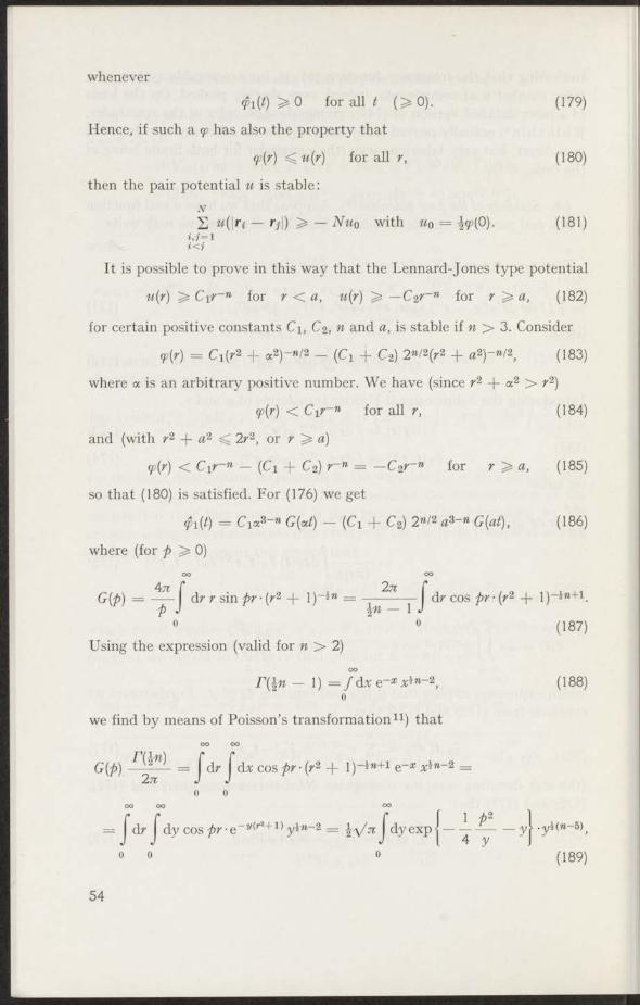
whenever(t) > 0 for all t (> 0 ) . (179)
Hence, if such a 9? has also the property that
(p{r) ^ u(r) for all r, (180)
then the pair potential u is stable:N2 w(|fi — f j I) > — Nuo with «o = i9>(0). (181)
i<iIt is possible to prove in this way that the Lennard-Jones type potential
u(r) ^ C\r~n for r < a, u(r) —C2r-n for r ^ a, (182)
for certain positive constants C1, C2, « and a, is stable if n > 3. Consider
9»(r) = Ci(r2 + a2)- ”/2 - (Ci 4- C2) 2»/2(r2 + a2)-»/2, (183)
where a is an arbitrary positive number. We have (since r2 a2 > r2)
<p(f) < Cir~B for all r, (184)
and (with r2 -f- a2 < 2r2, or r ^ a)
<p(r) < Cir~B — (Ci + C2) r ” = — C2r~” for r ^ a, (185)
so that (180) is satisfied. For (176) we get
0l(f) = Cia3-B G(ai) — (Ci + C2) 2»/2 a3~B G(a*), (186)
where (for p ^ 0)
G(p)An
0 0 0 0
■f dr r sin pr • (r2 + l)~lB = —- - - - f dr cos pr • (r2 + 1)-*B+1.J h ï — 1 J
Using the expression (valid for n > 2)OO
C(Jw — 1) = J dx e~x xin~2,0
we find by means of Poisson’s transformationu ) that
(187)
(188)
OO OOran)G ( f l . - ~ dr I dx cos pr-(r2 -f- 1)~*B+1 e~x xin~2
0 0OO OO
f 1 >2dr j dy cos pr-e~v<’T'+1 y*B_2 = | dy exp j — —-----'ƒ<0 0
yj> .y \ (n -b ) f
(189)
54
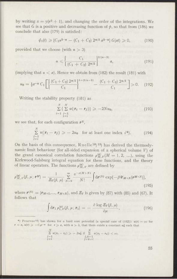
by writing x = y(r* 2 * * + 1 ) , and changing the order of the integrations. Wesee that G is a positive and decreasing function of p, so that from (186) weconclude that also (179) is satisfied:
<pi(t) > (Cia3-« — (Ci + C2) 2»/2 «3-»} G(at) > 0, (190)
provided that we choose (with n > 3)f C l 1 1/(»—3)
“ < I (Ci + C2) 2»/2 } *' (191)
(implying that a < a). Hence we obtain from (182) the result (181) with
, „ Tl (c i + c 2) 2»/2li+(3/„-3) ,c + c v 2„/2 -]| j i _ c T — I ~ ' U ± c r — J > a (192)
Writing the stabihty property (181) asN N
Z { 2 *(!»•< - *•ƒ!)} ^ — 2N u o , ( 193)i - i i - 11*1
we see that, for each configuration r^,NS M(lri — ril) ^ — 2mo for at least one index i*). (194)
l - il # i
On the basis of this consequence, R u e lle10) 13) has derived the thermodynamic limit behaviour (for all-sided expansion of a spherical volume V) ofthe grand canonical correlation functions p(m>v (M = 1 , 2 , ...), using theKirkwood-Salsburg integral equation for these functions, and the theoryof linear operators. The functions p%\ r are defined by
1 oo 0 —/ i (M + N ) /•
Pm. vW, /C *m) = -- , , , S ----- -------- d rw exp{ - ^ M+N(rM+N)},^ v [ p > f t) N = 0 ! J
(195)
where fW = (fM+i,-.., Tm+n ), and Sy is given by (87) with (85) and (67). Itfollows that
<w //» . -X 3 log B y if i , /*)J dfi P i,r \P > ri) = - - - - - - - - - - - g - - - - - - - - - , (196)
*) P e n r o s e 12) has shown for a hard core potential (a special case of (182)): u(r) = oo forr < a, u(r) > — Czr~» for r > a, w ith » > 3, th a t there exists a constant «ó such th a t
N N2 «(In — Tj I) > — 2«Ó if 2 «(In — rj,-|) < oo.
1=1 1,k— 11*1 1***1
55
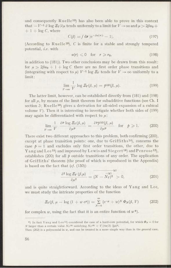
and consequently R u elle13) has also been able to prove in this contextthat — V~l 8 log Sy/S/t tends uniformly to a limit for V ->oo and ft > 2/Swo ++ 1 + log C, where
C(p) = / d r |e- ^ |r|) - 1|. (197)
(According to R u e lle10), C is finite for a stable and strongly temperedpotential, i.e. with
u(r) < 0 for r > ro, (198)
in addition to (181)). Two other conclusions may be drawn from this result:for n > 2/Smo + 1 + log C there are no first order phase transitions and(integrating with respect to ft) F -1 log Ey tends for V -*■ oo uniformly to alimit:
lim ~ log Ey(fi, ft) — (P, ft). (199)F-x» v
The latter limit, however, can be established directly from (181) and (198)for all [i, by means of the limit theorem for subadditive functions (see Ch. Isection 3; R u elle10) gives a derivation for all-sided expansion of a cubicalvolume V). Then it is interesting to investigate whether both sides of (199)may again be differentiated with respect to ft:
lim -L a » l°g S rtf .r t _ for p > hF-*» F 8ft'p 8ftP
There exist two different approaches to this problem, both confirming (200),except at phase transition points: one, due to G rif f ith s14), concerns thecase p = 1 and excludes only first order transitions, the other, due toY ang and Lee15) and improved by Lewis and S ie g e rt16) and P en ro se12),establishes (200) for all p outside transitions of any order. The applicationof Gri f f i ths ’ theorem (the proof of which is reproduced in the Appendix)is based on the fact that (cf. (150))
------------------------------ (r )
_ (Jv _ sfi, > o, (Mu8ft2
and is quite straightforward. According to the ideas of Yang and Lee,we must study the intricate properties of the function
OO
Sy(p, /t — log (1 + w e")) = 2 (e“" + W)N V) (202)iV=0
for complex w, using the fact that it is an entire function of w*).
*) In fact Yang and Lee16) considered the case of a hard-core potential, for which = OforN larger than a certain value AV*11' satisfying JVv(0) < F/(4ir/3) (Ja)s.Then (202) is a polynomial in w, and can be treated in a more simple way than in the general case.
56
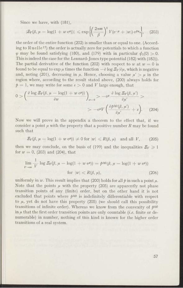
Since we have, with (181),
the order of the entire function (202) is smaller than or equal to one. (According to R u elle17) the order is actually zero for potentials to which a function<p may be found satisfying (180), and (179) with in particular $i(0) > 0.This is indeed the case for the Lennard-Jones type potential (182) with (183)).The partial derivative of the function (202) with respect to w at w = 0 isfound to be equal to exp fi times the function —8 log Sy/dfi, which is negativeand, noting (201), decreasing in f i . Hence, choosing a value / i ' > f j , in theregion where, according to the result stated above, (200) always holds forp = 1, we may write for some e > 0 and V large enough, that
( 8 log S v(fi, fi — log(l + w ef)) \ 8 log Sy(p, p')u > I --------------- ------------------I > — ------- —------>\ GW / ip=0 d/A
> — e**F ^ 8Pig)(P- V ) + ^ (204)
Now we will prove in the appendix a theorem to the effect that, if weconsider a point fi with the property that a positive number R may be foundsuch that
3y((i, ^ — log(l -f- w e )) 4 0 for \w\ < R((}, fi) and all V, (205)
then we may conclude, on the basis of (199) and the inequalities 3y > 1for w = 0, (203) and (204), that
„ 1hm —— log By(p, fi — log(l + w e )) = fi — log(l + w e"))
F -K X 3 Vfor \w\ < R(p, fi), (206)
uniformly in w. This result implies that (200) holds for all p in such a point fi.Note that the points fx with the property (205) are apparently not phasetransition points of any (finite) order, but on the other hand it is notexcluded that points where p(& is indefinitely differentiable with respectto fi, yet do not have this property (205) (we should call this possibilitytransitions of infinite order). Whereas we know from the convexity of p(&>in fi that the first order transition points are only countable (i.e. finite or denumerable) in number, nothing of this kind is known for the higher ordertransitions of a real system.
}. (203)f ( 'Ztiwi
\Sy((i, fi — log(l + w e^))| < exp ------ J F(e~*t + |w|) e^“o
57
A P P E N D IX 14) 12)
When a sequence of real convex functions <pn(x) (n oo, x real) tends toa limit
lim <pn(x) = <p(x), (A 1)n—*oo
then the limit function <p(x) is also convex, or, in other words, the firstderivatives <ph{x)(n —► oo) and 9/(2) are all increasing, each one with at mosta countable number of jump discontinuities. Moreover, as will be shownhere, we have
lim <ph(x) = 9/(2) (A 2)n-+oo
at every point where (p'{x) is continuous (G riffiths’ theorem14); the discreteness of the variable n in this appendix is not essential, it may be madecontinuous without any restrictions).Proof: Suppose that <p'(x) is continuous for x = Xo, but that (A 2) does
not hold at this point: in particular, assume that there is a numbere > 0 such that
<p'{x0) — <pn(x0) > s (A3)
for arbitrarily large values of n. This assumption will appear to contradict (A 1), Since <p'(x) is continuous at xq, we may find a number d > 0such that
\q>'(x) — 9/(20) 1 < if \x — *ol < ó(e). (A 4)
Now, as 95» (2) is increasing, (A 3) and (A 4) imply that
9/(2) — 9^(2) > 9/(2) — <pn(x0) > for Xo — 6(e) < 2 < 20. (A 5)
Integration of both sides of this inequality from 20 — <5 to 20 yields
{91(20) — 9>n(*0)} — {9571(20 — <5) — 95(20 — (5)} > P(e) e, (A 6)
(still for arbitrarily large values of n), so that <pn{x) does not convergeto 95(2) either at 20 or at 20 — <5. In the same way (considering 20 < 2 << 20 + <3) the assumption that 95'(20) — <ph(x0) < — e for arbitrarilylarge values of n leads to a contradiction, and we conclude that (A 2)is satisfied for 2 = 20.
The step from (A 5) to (A 6) uses the fact that a convex function is absolutely continuous and hence equal to the primitive function of its firstderivative. A proof which does not invoke this absolute continuity propertyhas been found by F ish e r18).
Consider next a sequence of complex functions <pn[w){n 00, w complex)which converges for real values of w. Let exp ncpn(w) be an entire function of
58
order < 1, to which independent of n a positive constant R may be foundsuch that it does not vanish for \w\ < /?. From the theory of entire functions19)we apply Hadamards’ factorization theorem and Jensen’s formula. If theorder of the entire function exp n<p„(w) is less than one, its factorization is
OO
exp n<pn(w) = exp n<p„(0) • ]J 0 — w/w*,»), (A 7)f c = t
where the Wk,n (k — \,2 , ...) are its zeros, with, as assumed,
|wic, n\ > R > 0 for all k and n. (A 8)
Comparing the power series expansion in w for 9on(w) following from (A 7),with the Taylor expansion of <pn(w) around the origin,
OO
<Pn{w) = Z wP<p^\0)lp\ (A 9)p=0
(which has a radius of convergence at least equal to R), we find that
1 °°<Pn\0)lp\ = — — S P > 1. (A 10)pn fc=i
Using this relation for p = 1, (A 7) may also be written asOO
exp tupn(w) = exp n{<pn(0) + w<pn{ 0)}- II (1 — W®*,») exp (w/wn,»), (All)* = l
in which form it is also the proper factorization if the order is equal to one(and (A 9) is only known to hold for p ^ 2). From Jensen’s formula wederive the inequality
FZ„(r')—-— dr < max log |exp n{<pn(w) — 9>„(0)}|, (A 12)
V |i» |=r
where Z n(r) is the number of the zeros Wk, n(k = 1,2, ...) with \wt, n\ ^ r(and hence, according to (A 8), vanishing for r smaller than at least the valueR). Now if for positive constants C\, C2 and C3 we have that
|exp n{(pn(w) — 9?„(0)}| < exp w(Ci + C2 \w\) for all n and w (A 13)
(a more detailed statement of the fact that exp nq>n[w) is entire of order^ 1) and
l9?n(0)| < C3 for all n, (A 14)then the limit
lim cpn(w) = cp{w) for real w (A 15)
59
may be extended to complex values of w :lim <pn{w) = (p(w) for \w\ < R, (A 16)n-+oo
uniformly.Proof'. From (A 12) and (A 13) it follows, using also the fact that Z n(r) is
positive and increasing in r, thate r
„ , f dr'Zn[?) — Zn(?)J ~ rr
er er
< J Znjs dr' < ƒ Zn , dr' < n(c i + c 2er). (A 17)r R
For the absolute values of the coefficients in the power series (A 9) wehave, according to (A 10), the inequality
\<P%\0)lp\\ < — 5 - — f r~P dZ n(r). (A 18)pn k=i pn JR
Here the Stieltjes integral may be integrated by parts if p > 2 (thenthe term at the upper boundary vanishes because of (A 17)), and with(A 17) we obtain
K W < 1 1 '" * ” 1 ¥ '> *■ < ^ + (j, - Ci') V ^ ’ * * 2B (A 19)
Consequently we have, using also (A 14),
00 f Ci C2 ei? 1 / ltt'1 V . , _I<Pn{w) ~ <P»(0)| < C3 |wj + S + J — [ \ \ l t ) f°r |W| < R ’
(A 20)or choosing a number & between 0 and 1,
#2\<PnM — 9?m(0)| < C3&R + (Ci + C2 eR) ------- for \w\ (A 21)1 — ifHence the sequence of functions cpn{w) — <fn(0){n -*■ 0 0 ), which according to (A 15) converges to <p(w) — q>(0) on the part of the real axiscontained in the circle \w\ = R, is also uniformly bounded in theinterior of this circle. In these circumstances the Vitali convergencetheorem19) may be applied, giving
lim {(pn{w) — <Pm(0)} = <p(w) — 99(0) for \w\ < êR (A 22)n —*oo
uniformly, which result implies (A 16).
60
The step from (A 15) and (A 21) to (A 22) was performed explicitly in thework of Y ang and L ee15). Then Lew is and S ieg er t16) realized that theVitali convergence theorem could be applied (their treatment, consideringthe case of the “pressure” formalism, is, however, unsatisfactory). The useof Jensen’s formula we owe to P en rose12).
REFERENCES
1) See e.g. Calien, H. B., Thermodynamics (New York and London, 1960).2) É hrenfest, P., Commun. Kamerlingh Onnes Lab. Univ. Leiden, Suppl. 75b (1933).3) See e.g. Farquhar, I. E., Ergodic Theory in Statistical Mechanics (London-New York-Sidney,
1964).4) B irkhoff, G. D., Proc. Nat. Acad. Sci. 17 (1931) 650, 656.5) K hinchin, A. I., Mathematical Foundations of Statistical Mechanics (New York, 1949).6) See e.g. Münster, A. in: Flügge, S., Handbuch der Physik III/2 (Berlin-Göttingen-Heidelberg,
1959).7) See e.g. K endall, M. G., The advanced Theory of Statistics I (London, 1952).8) Mazur, P. and Van der Linden, J., J. math. Phys. 4 (1963) 271.9) C hintschin, A. J., Mathematische Grundlagen der Quantenstatistik (Berlin 1956).
10) R uelle, D., Lectures in Theoretical Physics VI (Boulder 1963) 73.11) W atson, G. N., Theory of Bessel Functions (Cambridge, 1952).12) Penrose, O., J. math. Phys. 4 (1963) 1312.13) R uelle, D., Ann. Phys. (N.Y.) 25 (1963) 109.14) G riffiths, R. B., J. math. Phys. 5 (1964) 1215.15) Yang, C. N. and Lee, T. D., Phys. Rev. 87 (1952) 404.16) Lewis, M. B. and S iegert, A. J. F., Phys. Rev. 101 (1956) 1227.17) R uelle, D., Helv. phys. Acta 36 (1963) 183.18) Fisher, M. E., J. math. Phys. (to be published).19) See e.g. T itchm arsh, E. C., Theory of Functions (Oxford, 1939).
61

SAMENVATTING
In hoofdstuk I worden een aantal thermodynamische-limietproblemenonderzocht op grond van zeer algemene veronderstellingen omtrent dewisselwerking („stabiliteit” en „sterke afneming”). Hiermee wordt een bijdrage geleverd tot de fundering van de statistische thermodynamica. Nade inleidende paragrafen 1 en 2, volgt in 3 en 4 als belangrijkste onderdeelhet aantonen van de gelijkwaardigheid van het microkanonieke, het kano-nieke en het grootkanonieke formalisme. De bewijsmethode is een synthesevan ideeën van Fisher (gebruikmaking van de limietstelling voor subaddi-tieve functies) en Khinchin (toepassing van het centrale-limiettheoremauit de waarschijnlijkheidstheorie). In gewijzigde vorm wordt deze methodein paragraaf 5 aangewend voor het vaststellen van de asymptotische waardevan de microkanonieke temperatuur. Paragraaf 6 geeft een terugblik op deontwikkeling van het onderwerp sinds Khinchin’s behandeling. In deappendix wordt een hulpstelling bewezen.
In hoofdstuk II komen een aantal onderwerpen aan de orde die verbandhouden met het in hoofdstuk I behandelde probleem. In paragraaf 1 wordtde benodigde kennis van de thermodynamica uiteengezet. De paragrafen2 en 3 dienen om het beeld van het vraagstuk omtrent de fundering van deklassieke statistische physica volledig te maken. Paragraaf 4 geeft, op grondvan algemene limiettheorema’s uit de waarschijnlijkheidstheorie, de wiskundige voorbereiding op de (gedeeltelijk nieuwe) behandeling van Khinchin’s asymptotische resultaten voor een separabel systeem, die in paragraaf5 volgt. In paragraaf 6 en de appendix worden enige resultaten van derecente ontwikkeling op het gebied van thermodynamische-limietproblemen,in min of meer bewerkte vorm weergegeven.
62
Teneinde te voldoen aan het verzoek van de faculteit der Wiskunde enNatuurwetenschappen, volgt hier een overzicht van mijn studie.
In 1952, na het behalen van het diploma H.B.S.-B aan het Groen vanPrinsterer Lyceum te Vlaardingen, begon ik mijn studie in de faculteit derWiskunde en Natuurwetenschappen aan de Rijksuniversitèit te Leiden. Injuli 1955 legde ik het candidaatsexamen (richting a) af, en in april 1958slaagde ik voor het doctoraalexamen theoretische natuurkunde. In deperiode tussen beide examens deed ik ook praktisch werk, tot januari 1957op het Kamerlingh Onnes Laboratorium, en daarna op het Instituut-Lorentz. Dit betrof onderzoek op het gebied van, respectievelijk, de para-magnetische relaxatie en de thermodynamica der irreversible processen.
Mijn werkzaamheden op het Instituut-Lorentz als wetenschappelijkmedewerker van de Stichting voor Fundamenteel Onderzoek der Materie(F.O.M.-werkgroep M VI), zette ik sedertdien onder leiding van Prof. Dr.P. M azur voort, met onderzoek omtrent de grondslagen van de statistischephysica. De recente resultaten hiervan werden beschreven in dit proefschrift.
Publicaties:On the canonical distribution in quantum statistical mechanics
J. van der L inden and P. Mazur, Physica 27 (1961) 609.Asymptotic form of the structure function for real systems
P. M azur and J. van der L inden, J. math. Phys. 4 (1963) 271.On the asymptotic problem of statistical thermodynamics for a real system
J. van der L inden, Physica (wordt gepubliceerd).
63

ST EL LIN G EN
I
De thermodynamische limiet van de mikrokanonieke temperatuur voornen reëel systeem bestaat, en heeft de vereiste eigenschappen.
Dit proefschrift, hoofdstuk I § 5.
II
De gelijkwaardigheid van het mikrokanonieke en het kanonieke phase-gemiddelde van een somfunctie voor een separabel systeem, kan eenvoudigaangetoond worden m.b.v. een generalisatie van K h in ch in ’s asympto-tische evaluatie van de structuurfunctie van een dergelijk systeem.
A. I. K h in ch in , Mathematical Foundations of StatisticaMechanics.Dit proefschrift, hoofdstuk II § 5.
III
De stelling van D ini voor een monotone rij van functies geldt ook vooreen rij {<px(x)} met de eigenschap dat
N<pN(x) > N l9Kl{x) + (IV — Ni) (pn- n^x) als N > Ni.Dit proefschrift, hoofdstuk I appendix.
IV
Grif f i th s ’ bewijs van de gelijkwaardigheid van het mikrokanonieke en hetkanonieke formalisme in de quantumstatistische thermodynamica voor eenreëel systeem, is gedeeltelijk onbevredigend. Het bezwaar ertegen kan echteropgeheven worden door gebruik te maken van de voorgaande stelling.
R. B. G riffith s, J. math. Phys. 6 (1965) 1447.
V
De mogelijkheid van een pseudo-klassieke behandeling (m.b.v. Wigner-distributiefuncties) van het asymptotische probleem in de quantumstatis-tica, zoals verwezenlijkt voor een separabel systeem, komt niet in aanmerkingvoor een reëel systeem.
J. van der L inden and P. Mazur, Physica 27 (1961) 609.

VI
De bewering van Münster dat de door hem beschouwde statistischefuncties Si+i{z) voor alle waarden van l gehele functies zijn, is onjuist.
A. M ü n s te r , Z. Physik 136 (1953) 179; zie ook p. 384 in:S. F lü g g e , H andbuch der Physik III/2 .
VII
Het argument van Landau en Lifshitz, dat in een 1-dimensionaalsysteem evenwicht tussen twee verschillende homogene fasen onmogelijkzou zijn, is niet steekhoudend.
L. D. L a n d a u en E. M. L i f s h i tz , S tatistical Physics(p. 482).
VIII
De behandeling die Glarum geeft van de diëlectrische relaxatie inpolaire vloeistoffen bevat een verband tussen het in- en het uitwendigemacroscopische wisselveld, dat microscopisch gerechtvaardigd moet en kanworden.
S. H. G la ru m , J . chem. Phys. 33 (1960) 1371.
IX
Symmetrie-overwegingen en Onsager-relaties sluiten een kruis-effecttussen warmtegeleiding en viscositeit niet uit voor gassen bestaande uitniet-bolvormige molekulen, geplaatst in een magneetveld. Om te zien of diteffect een meetbare orde' van grootte heeft, is het van belang het werk vanKagan en Maksimov uit te breiden.
S. R. d e G ro o t and P. M a zu r, Non-equilibrium Therm odynamics.Y. K a g a n and L. M a k s im o v , Soviet Phys. J .E .T .P .14 (1962) 604.
X
Het door Van Leeuwen gegeven beeld van de wereldgeschiedenis isverwant met de ideeën omtrent de algemene evolutie van Tei lhard deChardin.
A. Th. v a n L e e u w e n , C hristianity in W orld H istory .T e i lh a r d d e C h a rd in , H et verschijnsel mens.


![[Spanos] Statistical Foundations of Econometric Modelling](https://img.pdfslide.us/doc/110x75/55cf8583550346484b8eda22/spanos-statistical-foundations-of-econometric-modelling.jpg)