Embed Size (px)
Citation preview

On the feasibility of cognitive radio
by
Niels Kang Hoven
B.S. (Rice University) 2003M.E.E. (Rice University) 2003
A thesis submitted in partial satisfactionof the requirements for the degree of
Master of Science
in
Engineering - Electrical Engineering and Computer Sciences
in the
GRADUATE DIVISION
of the
UNIVERSITY OF CALIFORNIA, BERKELEY
Committee in charge:
Professor Anant Sahai, ChairProfessor Kannan Ramchandran
Spring 2005

The thesis of Niels Kang Hoven is approved.
Chair Date
Date
University of California, Berkeley
Spring 2005

On the feasibility of cognitive radio
Copyright c© 2005
by
Niels Kang Hoven

Abstract
On the feasibility of cognitive radio
by
Niels Kang Hoven
Master of Science in Engineering - Electrical Engineering and Computer Sciences
University of California, Berkeley
Professor Anant Sahai, Chair
In this thesis we explore the idea of using cognitive radios to reuse locally unused spectrum
for their own transmissions. Cognitive radio refers to wireless architectures in which a
communication system does not operate in a fixed band, but rather searches and finds an
appropriate band in which to operate. We impose the constraint that they cannot generate
unacceptable levels of interference to licensed systems on the same frequency and explore
the fundamental requirements for such a system.
We first show that in order to deliver real gains, cognitive radios must be able to
detect undecodable signals. This is done by showing how to evaluate the tradeoff between
secondary user power, available space for secondary operation, and interference protection
for the primary receivers. We prove that in general, the performance of the optimal detector
for detecting a weak unknown signal from a known zero-mean constellation is like that of
the energy detector (radiometer). However, we show that the presence of a known pilot
signal can help greatly.
Using received SNR as a proxy for distance, we prove that a cognitive radio can vary
its transmit power while maintaining a guarantee of non-interference to primary users.
We consider the aggregate interference caused by multiple cognitive radios and show that
aggregation causes a change in the effective decay rate of the interference. We examine
1

the effects of heterogeneous propagation path loss functions and justify the feasibility of
multiple secondary users with dynamic transmit powers. Finally, we prove the fundamental
constraint on a cognitive radio’s transmit power is the minimum SNR it can detect and
explore the effect of this power cap.
Professor Anant SahaiThesis Committee Chair
2
Contents
Contents i
List of Figures iii
List of Tables v
Acknowledgements vi
1 Introduction 1
1.1 Spectrum allocation vs. usage . . . . . . . . . . . . . . . . . . . . . . . . . . 1
1.2 The policy debate . . . . . . . . . . . . . . . . . . . . . . . . . . . . . . . . 2
1.3 Increasing spectrum efficiency . . . . . . . . . . . . . . . . . . . . . . . . . . 3
1.4 Software-defined radios . . . . . . . . . . . . . . . . . . . . . . . . . . . . . . 5
1.5 Cognitive radios . . . . . . . . . . . . . . . . . . . . . . . . . . . . . . . . . 6
1.6 Overview . . . . . . . . . . . . . . . . . . . . . . . . . . . . . . . . . . . . . 7
2 Interference 9
2.1 Protecting privileged users . . . . . . . . . . . . . . . . . . . . . . . . . . . . 9
2.2 Shadowing effects . . . . . . . . . . . . . . . . . . . . . . . . . . . . . . . . . 12
2.3 Shadowing uncertainty vs. primary receiver uncertainty . . . . . . . . . . . 14
2.4 Interference suppression through decodability . . . . . . . . . . . . . . . . . 17
3 Detection 19
3.1 Background . . . . . . . . . . . . . . . . . . . . . . . . . . . . . . . . . . . . 20
3.2 Detection of undecodable BPSK signals . . . . . . . . . . . . . . . . . . . . 21
3.3 Detection of zero-mean constellations . . . . . . . . . . . . . . . . . . . . . . 22
3.3.1 Model . . . . . . . . . . . . . . . . . . . . . . . . . . . . . . . . . . . 22
i

3.3.2 Results . . . . . . . . . . . . . . . . . . . . . . . . . . . . . . . . . . 23
3.3.3 Analysis . . . . . . . . . . . . . . . . . . . . . . . . . . . . . . . . . . 23
3.4 Pilot signals and training sequences . . . . . . . . . . . . . . . . . . . . . . . 25
4 Power control 26
4.1 Related work . . . . . . . . . . . . . . . . . . . . . . . . . . . . . . . . . . . 27
4.2 Model . . . . . . . . . . . . . . . . . . . . . . . . . . . . . . . . . . . . . . . 28
4.3 SNR as a proxy for distance . . . . . . . . . . . . . . . . . . . . . . . . . . . 29
4.4 Out-of-system interference . . . . . . . . . . . . . . . . . . . . . . . . . . . . 32
4.5 Single secondary transmitter . . . . . . . . . . . . . . . . . . . . . . . . . . 33
4.6 Single secondary transmitter with shadowing/fading . . . . . . . . . . . . . 36
4.7 Multiple licensed secondary transmitters . . . . . . . . . . . . . . . . . . . . 37
4.8 Multiple dynamic secondary transmitters . . . . . . . . . . . . . . . . . . . 39
4.9 Minimum detectable SNR . . . . . . . . . . . . . . . . . . . . . . . . . . . . 41
5 Conclusion 46
Bibliography 49
References . . . . . . . . . . . . . . . . . . . . . . . . . . . . . . . . . . . . . . . . 49
A Capacity calculations 51
B Allocated spectrum for communications 53
ii
List of Figures
1.1 There is a great discrepancy between spectrum allocation and spectrum usage. . . . . . 2
1.2 What if the government regulated acoustic spectrum the way it regulates radio spectrum? 4
1.3 What if the government regulated public roads the way it regulates public airwaves? . . 5
2.1 For practical spectrum reuse, legacy users near the decodability limit must accept some
signal loss. Guaranteeing protection to primary users too close to the decodability border
results in a large no-talk zone. . . . . . . . . . . . . . . . . . . . . . . . . . . . . 10
2.2 The size of the necessary no-talk zones depends on the transmission power of the secondary
user . . . . . . . . . . . . . . . . . . . . . . . . . . . . . . . . . . . . . . . . . 11
2.3 If we don’t know exactly where the primary receivers are, we must protect everywhere they
might possibly be. We can still reclaim plenty of spectrum in the middle of nowhere. . . 12
2.4 A secondary transmitter who cannot tell if he is in a shadow must hear a much weaker
signal to be sure he will not interfere. . . . . . . . . . . . . . . . . . . . . . . . . . 13
2.5 “Pollution” from the primary transmissions limits the rate of secondary systems very close
to it. However, the regime rapidly becomes interference limited as systems move further
from the transmitter. If primary receivers are sparse, much usable real estate could be
reclaimed if the uncertainty in their locations was removed. The dotted line at 60 m
denotes the approximate limit of decodability. . . . . . . . . . . . . . . . . . . . . 15
2.6 Overcoming uncertainty, whether in the location of the primary receivers, or in shadowing,
allows useful real estate to be reclaimed. (Figures not to scale) . . . . . . . . . . . . . 16
3.1 Samples (N) required to detect a signal with a predetermined probability of error. With no
pilot signal present, an optimal detector performs only marginally better than an energy
detector. If a weak pilot signal is present, far fewer samples are necessary for detection. . 22
3.2 Samples (N) required to detect a signal with a predetermined probability of error. For a
zero-mean constellation, the energy detector is nearly optimal. . . . . . . . . . . . . . 24
4.1 SNR margins can be used as a proxy for distance . . . . . . . . . . . . . . . . . . . 31
iii
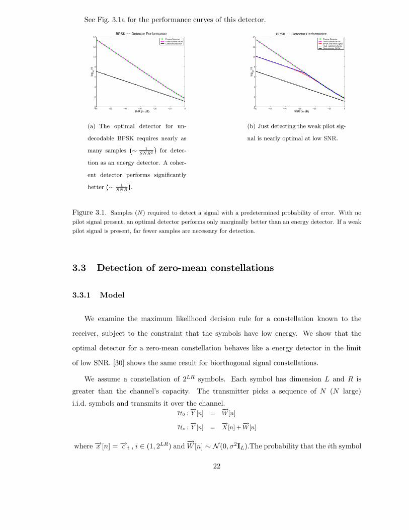
4.2 Interference from secondary transmitters increases towards the border of the protected
region. The secondary sea begins at 5100 m, at which point the interference becomes
infinite. . . . . . . . . . . . . . . . . . . . . . . . . . . . . . . . . . . . . . . . 32
4.3 Maximum power for a secondary transmitter vs. dB beyond rdec. ∆ measures the primary
signal attenuation from the transmitter to the decodability radius. For reference, we also
give the distance to the decodability radius, assuming attentuation as r−3.5 (i.e. α1 = 3.5). 43
4.4 The possibility of 10 dB of shadowing results in a 10 dB shift of the required SNR margin
(eqn. 4.10). . . . . . . . . . . . . . . . . . . . . . . . . . . . . . . . . . . . . . 44
4.5 A circular coast looks like a straight line to primary users near the edge of the protected
radius. . . . . . . . . . . . . . . . . . . . . . . . . . . . . . . . . . . . . . . . 44
4.6 The upper (eqn. 4.14) and lower (eqn. 4.12) bounds have the same decay exponent.
Approximating the coast of the secondary sea with a straight line is accurate to within a
constant. . . . . . . . . . . . . . . . . . . . . . . . . . . . . . . . . . . . . . . 45
4.7 (a) More aggressive power control rules (eqn. 4.20) require a lower density of secondary
transmissions near the protected region. (b) If the margins are too small, secondary users
are excessively constrained. . . . . . . . . . . . . . . . . . . . . . . . . . . . . . 45
A.1 We assume regular, hexagonal cells. . . . . . . . . . . . . . . . . . . . . . . . . . . 51
iv

List of Tables
4.1 For large ∆ (large primary transmit distances) small SNR margins correspond to large
physical distances. We assume attenuation as r−4 . . . . . . . . . . . . . . . . . . . 32
4.2 If the signal attenuates as r−2 the distances are even larger. . . . . . . . . . . . . . . 32
B.1 Spectrum under 3 GHz . . . . . . . . . . . . . . . . . . . . . . . . . . . . . . . 53
B.2 Microwave bands (609 MHz) . . . . . . . . . . . . . . . . . . . . . . . . . . . . . 54
B.3 Broadcast bands (423 MHz) . . . . . . . . . . . . . . . . . . . . . . . . . . . . . 54
B.4 Satellite bands (188 MHz) . . . . . . . . . . . . . . . . . . . . . . . . . . . . . . 54
B.5 Point-to-Multipoint bands (203 MHz) . . . . . . . . . . . . . . . . . . . . . . . . 55
B.6 PCS/Cellular bands (193 MHz) . . . . . . . . . . . . . . . . . . . . . . . . . . . 55
B.7 Unlicensed bands (110 MHz) . . . . . . . . . . . . . . . . . . . . . . . . . . . . . 56
v

Acknowledgements
Many thanks to Anant Sahai for his guidance and patience, to Kannan Ramchandran for
making the time to be on my committee, to Rahul Tandra for his helpful suggestions, to
Ruth Gjerde for caring, to the many authors of this template for saving me hours of work,
and everyone else whose support and encouragement helped me survive a very, very long
semester.
vi
Curriculum Vitæ
Niels Kang Hoven
Education
2003 Rice University
B.S., Electrical and Computer Engineering
2003 Rice University
M.E.E., Electrical and Computer Engineering
2005 University of California Berkeley
M.S., Engineering - Electrical Engineering and Computer Sciences
Personal
Born January 19, 1981, Washington, D.C.
Niels grew up in Montgomery County, MD, where he spent the carefree days of youth
swimming and playing the clarinet. The men’s swim team at Rice was disbanded the year
he arrived, so Niels joined Rice’s water polo and crew teams instead. During a semester
in Australia, he became an accomplished rock climber, but returned to Rice in time to
compete on his college’s Beer-Bike team, twice as a biker and once as a chugger. Following
graduation he continued his westward migration, eventually ending up in Berkeley, CA.
There, he continued his training in the gentle art of Brazilian jiu-jitsu, completed the
Escape from Alcatraz triathlon, and ate two Thanksgiving dinners in one day. Niels is a
member of Phi Beta Kappa, Tau Beta Pi, Eta Kappa Nu, and the Bullshido.com Hall of
Fame. In his spare time, he hopes to complete a Ph.D. in electrical engineering.
vii

viii

Chapter 1
Introduction
1.1 Spectrum allocation vs. usage
Traditionally, the FCC has allocated spectrum bands to a single use, issued exclusive
licenses to a single entity within a geographical area, and prohibited other devices from
transmitting significant power within these bands. Looking at the NTIA’s chart of these
frequency allocations (Figure 1.1a), it appears that we are in danger of running out of
spectrum [1]. However, allocation is only half the story. Contrary to popular belief, actual
measurements (taken in downtown Berkeley, CA) show that most of the allocated spectrum
is vastly underutilized (Figure 1.1b) [2].
The Berkeley Wireless Research Center reports that 70% of the spectrum under 3 GHz
is available at any specific location and time. Under the FCC’s “exclusive rights” model of
frequency band ownership, if a licensed system is not transmitting, its spectrum remains
off-limits to other users.
To put this available spectrum in perspective, imagine that you wanted to build a
network of transmitters that would blanket an area with streaming DVD-quality video.
The maximum combined bit rate for the video and audio streams on a DVD is 9.8 Mbps.
Commercial DVDs generally encode their video streams around 5 Mbps. With 100 mW
1

(a) The NTIA’s spectrum allocation chart makes avail-
able spectrum look scarce.
(b) Measurements from the Berkeley Wireless Re-
search Center show the allocated spectrum is vastly
underutilized.
Figure 1.1. There is a great discrepancy between spectrum allocation and spectrum usage.
transmitters (the same as a typical wireless access point) placed 1 km apart, a data rate of
20 Mbps can be achieved through 85 MHz of free spectrum (Appendix A).
Examining solely the 402 MHz allocated to broadcast TV (Appendix B), if we assume
70% of the spectrum is available, we can fit two of these systems operating simultaneously
inside the broadcast TV spectrum. The available spectrum up to 3 GHz would fit 20
systems, blanketing an area with 160 DVD-quality video streams from low-powered wireless
transmitters.
1.2 The policy debate
Clearly, the spectrum is far from fully utilized. As a result, the FCC’s exclusive-use
allocation policy is being increasingly viewed as outdated. Opinions on the appropriate
solution, however, vary.
Some economists argue that the development of a secondary market in spectrum would
eliminate or greatly reduce the inefficiencies in spectrum usage [3], [4]. The FCC initiated
their current system of auctioning spectrum to the highest bidder under the assumption
2

that an efficient market would result in the spectrum being allocated to its most valuable
use. However, the exclusive-use policy rules out the shared spectrum bands that have led
to the recent explosion of unlicensed devices such as 802.11 wireless access points. Many
economists believe that allowing spectrum owners to resell their bands to secondary users
would solve this problem. An FCC policy statement reads, “An effectively functioning
system of secondary markets would encourage licensees to be more spectrum efficient by
freely trading their rights to unused spectrum capacity, either leasing it temporarily, or on
a longer-term basis, or selling their rights to unused frequencies” [5].
Opponents of secondary markets tend to favor a digital commons solution [6]. By
removing licensing barriers to spectrum use, a commons environment would encourage
innovation and maximize spectrum utility. Commons proponents argue that the astonishing
success of wireless networking devices is proof that unlicensed (or flexibly-licensed) devices
can coexist in a largely unregulated band. They assert that “wireless transmissions can be
regulated by a combination of (a) baseline rules that allow users to coordinate their use,
to avoid interference-producing collisions, and to prevent, for the most part, congestion, by
conforming to equipment manufacturer’s specifications, and (b) industry and government-
sponsored standards” [6]. Recognizing the need for increased spectrum efficiency, a number
of organizations such as New America, the Center for Digital Democracy, and Free Press,
have thrown their support behind spectrum deregulation [7]. However, further research is
required to lay the groundwork for the technology that policy makers on both sides assume
already exists.
1.3 Increasing spectrum efficiency
Presumably, whether a secondary markets policy, a commons policy, or some combina-
tion thereof is adopted, devices accessing this released spectrum will be required to do so
subject to some requirement of non-interference to incumbents. Signal detection is therefore
fundamental to both courses of action. This could refer to an unlicensed device deciding if a
particular frequency band is unused, or a spectrum owner deciding whether the extra inter-
3

ference he’s noticing is a misbehaving secondary licensee or just random noise fluctuations.
Arguments from both sides tend to address this as a solved problem, but that is not entirely
justified. In chapters 3 and 4 we address this detection problem and its ramifications.
Another common assumption is that technological advances will allow devices to coexist
without serious penalty. The idea is, “Is it really interference if nobody notices?” Like
children taking a shortcut across a neighbor’s yard, it seems reasonable to allow devices
to use a spectrum band if they can do so without interfering with the spectrum owner’s
devices. Designing wireless devices that can accomplish this remains a topic of current
research.
One strategy would permit devices to transmit on frequencies that are actively being
used by legacy/priority systems. However, the unlicensed devices would “whisper” at very
low power so as not to interfere with the spectrum owner (Figure 1.2). This is the approach
taken by ultra-wideband systems, which spread their power over a huge bandwidth to
minimize the interference they cause other systems [8].
Figure 1.2. What if the government regulated acoustic spectrum the way it regulates radio spectrum?(Reprinted with permission. [9])
An alternative strategy would have the unlicensed device transmit only on frequencies
4

Figure 1.3. What if the government regulated public roads the way it regulates public airwaves?(Reprinted with permission. [9])
which are locally or temporally unused (like borrowing someone’s summer home during the
winter months). This has the advantage that the unlicensed devices can use much more
power in a narrow bandwidth, but they must be able to determine which frequency bands
are available [10]. Cognitive radios take this approach, dynamically adjusting their trans-
missions in response to their environment [11], [12]. By scavenging unused (or underused)
bands, cognitive radios (section 1.5) can increase the efficiency of our current spectrum
usage (Figure 1.3).
1.4 Software-defined radios
When policy makers refer to “communications technologies that rely on processing
power and sophisticated network management, instead of raw transmission power, to pre-
vent interference” [6] they are laying their faith in emerging technologies such as software-
defined radio (SDR). The FCC describes a software-defined radio as “a radio that includes
a transmitter in which the operating parameters of frequency range, modulation type or
5

maximum output power (either radiated or conducted), or the circumstances under which
the transmitter operates in accordance with Commission rules, can be altered by making
a change in software without making any changes to hardware components that affect the
radio frequency emissions” [13]. In short, an SDR is capable of changing its transmissions
on the fly, rather than being bound by hardware constraints.
Simple SDRs are already being put to practical use. A dual-mode cell phone, for
example, switches between analog and digital transmissions depending on the strength of
the signals it receives. However, these phones have the capability to switch between only two
hardware-defined modes. Intel and others are actively developing the hardware to support
more advanced software-defined radios [14]. The eventual goal of SDR is to implement
the radio as fully-reconfigurable signal-processing software running on top of a flexible
hardware interface. SourceForge’s Open SDR and the GNU Radio project, for example,
attempt to “get a wide band ADC as close to the antenna as is convenient, get the samples
into something we can program, and then grind on them in software” [15]. Among other
applications, the GNU Radio can be an AM receiver [16], an FM receiver [17], an HDTV
receiver [18], or a spectrum analyzer [19]. SDR’s potential as a platform for cognitive radio
is especially exciting.
1.5 Cognitive radios
Cognitive radios, or “smart radios”, are likely to be constructed from the next generation
of software-defined radios. The FCC defines a cognitive radio as “a radio that can change its
transmitter parameters based on interaction with the environment in which it operates” [12].
They also point out that “the majority of cognitive radios will probably be SDRs, but neither
having software nor being field reprogrammable are requirements of a cognitive radio” [12].
The idea behind cognitive radio is that cognitive users will actively search the spectrum
for available frequency bands, dynamically adjusting their transmissions so as to avoid
interference with other users. These users could be legacy systems or other cognitive devices.
Cognitive radio is frequently cited by policy analysts as a powerful argument against the
6

exclusive-use spectrum model [7], [20], and it is one of the ideas currently being pursued
under the umbrella of DARPA’s Next Generation (XG) program [21].
Nevertheless, fundamental questions of cognitive radio’s practicality still remain open.
First, can practical cognitive systems even operate without causing excessive interference
to legacy users? Proving so is essential to convincing the FCC to open more spectrum
to “flexibly licensed” devices. Second, can useful wireless systems operate under these
constraints? In this thesis we target the former issue, focusing on non-interference to the
primary system rather than realizable benefits for secondary systems. We show the existence
of constraints that allow multiple cognitive radios to transmit at reasonable power levels
while maintaining a guarantee of service to legacy/priority users on the same band. We do
not consider achievable data rates or necessary protocols for the secondary systems.
1.6 Overview
In this thesis we explore the idea of using cognitive radios to reuse locally unused
spectrum for their own transmissions. The FCC will not allow new devices into already
allocated bands without a strong guarantee of non-interference to legacy users. We examine
the consequences of this requirement.
We impose the constraint that the cognitive radios cannot generate unacceptable levels
of interference to priority/legacy systems on the same frequency. To accomplish this, a
cognitive radio must first detect whether a frequency band is in use. Assuming the band is
spatially and/or temporally available, the radio may begin transmitting on it. Its maximum
transmit power will be constrained by a number of factors, however, including proximity
to the primary system, rate of propagation path loss, other cognitive radios, its minimum
detectable SNR, and licensing issues.
In Chapter 2, we prove that practical cognitive radios must be able to detect the presence
of undecodable signals [22]. We introduce the idea of protecting the primary system by
declaring “no-talk” zones for the secondary system. We discuss the effects of shadowing,
receiver uncertainty and transmit power on the size of these “no-talk” regions and show
7
that the border between the “no-talk” and “talk” zones for the secondary system may occur
beyond the primary system’s decodability limit.
In Chapter 3, we examine fundamental limitations on the detection of undecodable
signals. In section 3.2 we examine the number of samples required to detect, subject to
a fixed probability of error constraint, a decodable signal vs. an undecodable signal. We
show that a radiometer performs far worse than a coherent detector, and that the optimal
detector for unknown symbols from a zero-mean constellation behaves qualitatively like a
radiometer.
To make matters worse, slight uncertainty in the noise causes serious limits in detectabil-
ity [23], [24]. These barriers can be overcome if the licensed (primary) transmitter transmits
a perfectly known pilot signal or training sequence to aid detection. Coherent detection via
a matched filter results in processing gain and more effective signal detection.
Furthermore, pilots allow users to measure the local SNR of the primary signal, which
can then be used as a proxy for distance from the primary transmitter. Armed with this
information, cognitive radios (secondary users) can approximate their distance from the
primary transmitter and adjust their transmit power accordingly. In this thesis we present
an example of a power control rule which allows secondary users to aggressively increase
their transmit powers while still maintaining an acceptable level of aggregate interference
at the primary receivers.
In Chapter 4, we derive necessary conditions for a guarantee of non-interference to
primary users. Using received SNR as a proxy for distance, we prove that a cognitive radio
can vary its transmit power while maintaining this guarantee [25]. Of particular concern
are the effect of different propagation path losses for different systems, the effect of multiple
cognitive users, and the effect of heterogeneous transmit powers among the cognitive users.
We show that none of these concerns invalidates cognitive radio’s feasibility.
8

Chapter 2
Interference
Some of the most promising bands for unlicensed devices are the TV broadcast bands.
The FCC has already released a Notice Of Proposed Rule Making exploring the operation
of unlicensed devices on spatially/temporally “unused” television broadcast bands [26]. We
focus on these TV bands as a starting point for our models.
We begin with a motivating example to illustrate the necessity of detecting undecodable
signals. A naive designer might build a cognitive radio that falls silent if it can decode
the primary system’s transmission and talks otherwise. We will show that this rule is
inadequate. For simplicity, we begin by considering the case of a single cognitive radio
transmitter with a known maximum transmit power.
2.1 Protecting privileged users
In our model, we assume a band already potentially assigned to a high-powered single-
transmitter system (television, for example). All transmissions are assumed to be omnidi-
rectional. Figure 2.1a depicts a transmitter from the primary system. The dotted circle
represents the boundary of decodability for a single-transmitter system. That is, in the
absence of all interference, a user within the dotted line would be able to decode a signal
from the transmitter, while a user outside the circle would not. Our goal when introducing a
9

cognitive radio system is to maintain a guarantee of service to legacy users. We can control
the interference experienced by a primary receiver by declaring a “no-talk” zone around it,
within which the secondary transmitter is constrained to be silent. (This idea is examined
in detail in Chapter 4)
A
(a) The protected re-
gion (shaded area) can-
not extend all the way
to the decodability bor-
der (dotted line)
B
(b) If the protected region is too close
to the decodability border, receivers’
required no-talk zones grow large
Figure 2.1. For practical spectrum reuse, legacy users near the decodability limit must accept some signal
loss. Guaranteeing protection to primary users too close to the decodability border results in a large no-talk
zone.
However, if we want to actually create a system in which we guarantee performance to
every primary user within the decodability circle, we run into a problem. Primary users
(depicted with capital letters in the figures) on the very edge of the decodability region will
suffer under any change to the exclusive-use model. Consider receiver A, located on the
border of the decodability region (Figure 2.1a). Any amount of interference, no matter how
infinitesimal, will cause A to lose its ability to decode. Its no-talk zone must include the
entire world!
Therefore, it is clear that we must build some sort of buffer into our protected radius.
Let the shaded circle represent the “protected region” where we guarantee decodability to
primary receivers. Within this protected radius, all unshadowed primary receivers must be
10

guaranteed reception, even when the cognitive radios are operating. The more we shrink
the bound of the protected region inside the decodability region, the smaller the necessary
no-talk zones become. Conversely, we cannot protect everybody. As the protected radius
approaches the limit of decodability, the no-talk zones grow dramatically (Figure 2.1b).
The size of the no-talk zones also depend on the cognitive radio’s maximum transmit
power. If the secondary user is a “mouse” (Figure 2.2a), who squeaks softly with low power
transmissions, then the no-talk zones around each receiver can be much smaller. If it is a
“lion” (Figure 2.2b), roaring with high power transmissions, the radii of the no-talk zones
will become much larger.
C
(a) A small no-talk zone
protects a receiver against
quiet “mice”
C
(b) Receivers require larger
no-talk zones for roaring “li-
ons”
Figure 2.2. The size of the necessary no-talk zones depends on the transmission power of the secondary
user
Considering broadcast television, we see there will likely be no practical way for a
cognitive radio to know where the primary system’s receivers are located. As a result,
secondary users must stay out of the area that is the union of all possible no-talk zones (2.3a).
Even if the individual no-talk zones are small, this uncertainty in the primary receivers’
locations can result in a large global no-talk zone. We note that in the hypothetical example,
the prohibited region for the secondary user has already extended beyond the decodability
region.
Though it may at first seem problematic that the required quiet zones are so large,
11

C
(a) We protect all possible receiver
locations
(b) Still plenty of re-
claimable space
Figure 2.3. If we don’t know exactly where the primary receivers are, we must protect everywhere they
might possibly be. We can still reclaim plenty of spectrum in the middle of nowhere.
we remind the reader that our goal was to increase the spectrum available to users in the
middle of nowhere. These users are still well outside the quiet zones (2.3b).
2.2 Shadowing effects
If we take shadowing with respect to the primary transmitter into account (Figure 2.4a),
the prohibited region continues to grow. If a secondary user (depicted with lowercase letters
in the figures) detects a low SNR signal (Figure 2.4b), it has no way to tell if it is well outside
the protected region (user a), or in the global quiet zone but behind a building (user b). An
identical problem occurs as a result of multipath fading, which is discussed in Chapter 4.
To avoid locally shadowed secondary users interfering with unshadowed primary users (user
C), the no-talk zone must be pushed out even further. The outermost circle represents the
quiet zone such that the maximum SNR on its border equals the minimum SNR within the
unshadowed case’s protected region.
12

����
����
��������
������
������
������������
������������
������
������
���
���
(a) Some secondary systems
may be shadowed with re-
spect to the primary trans-
mitter
C��������
��������
����
����
������
������
��������
����
����
������
������
b
a
(b) The possibility of shadowing forces a larger no-talk
zone
Figure 2.4. A secondary transmitter who cannot tell if he is in a shadow must hear a much weaker signal
to be sure he will not interfere.
13

2.3 Shadowing uncertainty vs. primary receiver uncertainty
It is worth mentioning that shadowing causes in some sense a more “serious” penalty
than primary receiver uncertainty (Figure 2.6). To illustrate the difference between these
two scenarios, we will assume a broadcast TV transmitter with a decodability radius 52
km away. We also assume the signal decays as r−3.5. (This example is examined in much
greater detail in Chapter 4.) For simplicity, we assume the protected region ends just inside
the decodability radius and the no-talk zone begins just outside.
Uncertainty in the locations of the primary receivers is what forces us to combine the
individual no talk zones around each receiver into one large no-talk zone around the entire
protected region. If secondary users knew where the individual protected receivers were
located, it’s possible that there could be unpopulated areas within the protected radius
where secondary users could transmit without interfering with anyone. The worst case
penalty for receiver uncertainty occurs when there are no primary receivers at all, but the
the secondary users are forced to respect the protected area anyway. In this case, knowing
where primary receivers are (or aren’t) opens up the entire protected region for secondary
usage, reclaiming π522 ≈ 8400 km2 of land which would otherwise be underutilized.
If a secondary user could possibly be in a 10 dB shadow with respect to the primary
transmitter, he must detect a 10 dB weaker signal to be sure he is far enough away from
the protected users. This pushes the effective no-talk zone out by 10 dB, from 52 km to 100
km. Secondary users who could tell when they were in a shadow would be able to reclaim
this region1, which measures π1002 − π522 ≈ 23, 000 km2.
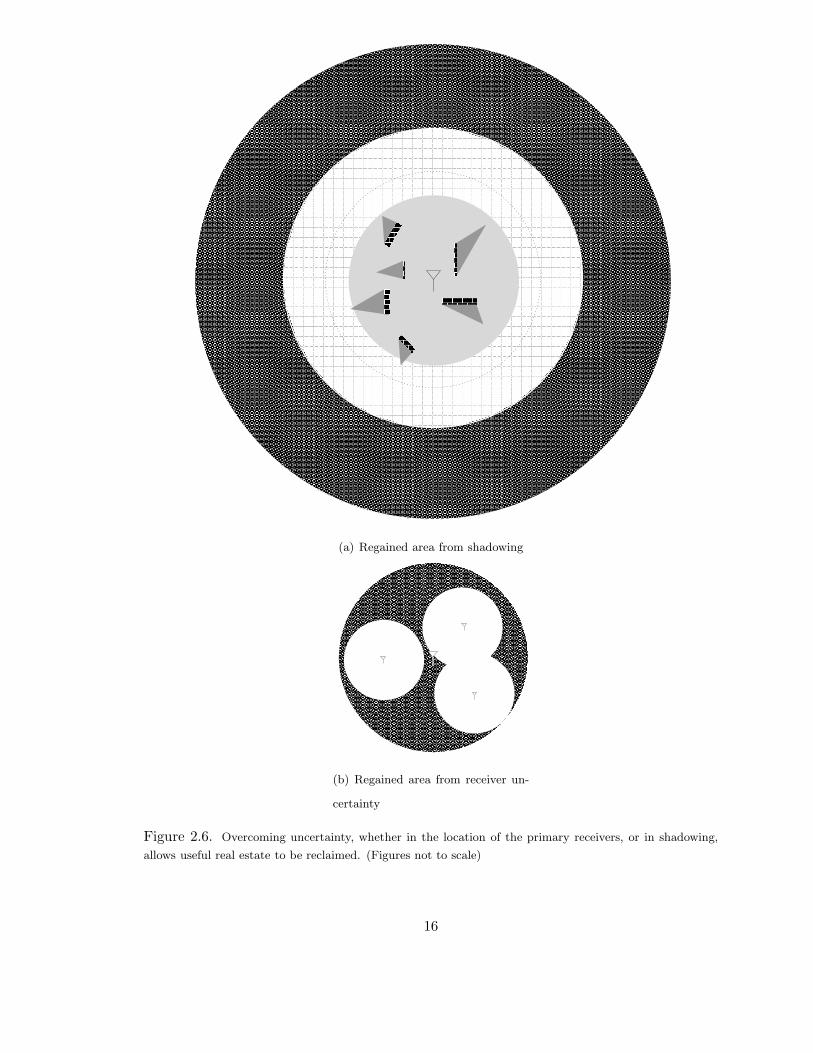
In this example, overcoming mild shadowing reclaims nearly 3 times as much area as
does knowing the primary receivers’ locations. It is also worth mentioning that the area
gained by knowing the receivers’ locations is “polluted” with transmissions from the primary
transmitter, making it slightly less valuable for secondary systems.
Consider a primary system transmitting at 100 kW. A secondary receiver r meters from
1Actually, it could be even more. If he can determine that he is shadowed with respect to the primaryreceivers, his required no-talk radius could shrink even further - perhaps even to inside the decodabilityradius!
14

the primary transmitter wishes to receive data from a 100 mW secondary transmitter 10 m
away. We assume free space path loss. Figure 2.5 shows that while users very close to the
primary transmitter are severely limited, most of the geographic area remains valuable for
secondary use.
0 20 40 60 80 1000
20
40
60
80
100
120
140
160
Distance from primary transmitter (km)
Cap
acity
(M
bps)
Capacity of 100 mW, 10 m range system vs. distance from primary transmitter
isolated secondary systemwith inteference from secondary 50m away
Figure 2.5. “Pollution” from the primary transmissions limits the rate of secondary systems very close to
it. However, the regime rapidly becomes interference limited as systems move further from the transmitter.
If primary receivers are sparse, much usable real estate could be reclaimed if the uncertainty in their locations
was removed. The dotted line at 60 m denotes the approximate limit of decodability.
This area is slightly less valuable than that gained by reducing shadowing uncertainty.
If a cognitive radio can determine that he is not shadowed with respect to the primary
transmitter, the real estate gained is in an area where the primary transmission is even
further attenuated (Figure 2.6).
Further research into methods of locating primary receivers or mitigating the necessary
margin for shadowing/fading is therefore extremely important.
15
��������������������������������������������������������������������������������������������������������������������������������������������������������������������������������������������������������������������������������������������������������������������������������������������������������������������������������������������������������������������������������������������������������������������������������������������������������������������������������������������������������������������������������������������������������������������������������������������������������������������������������������������������������������������������������������������������������������������������������������������������������������������������������������������������������������������������������������������������������������������������������������������������������������������������������������������������������������������������������������������������������������������������������������������������������������������������������������������������������������������������������������������������������������������������������������������������������������������������������������������������������������������������������������������������������������������������������������������������������������������������������������������������������������������������������������������������������������������������������������������������������������������������������������������������������������������������������������������������������������������������������������������������������������������������������������������������������������������������������������������������������������������������������������������������������������������������������������������������������������������������������������������������������������������������������������������������������������������������������������������������������������������������������������������������������������������������������������������������������������������������������������������������������������������������������������������������������������������������������������������������������������������������������������������������������������������������������������������������������������������������������������������������������������������������������������������������������������������������������������������������������������������������������������������������������������������������������������������������������������������������������������������������������������������������������������������������������������������������������������������������������������������������������������������������������������������������������������������������������������������������������������������������������������������������������������������������������������������������������������������������������������������������������������������������������������������������������������������������������������������������������������������������������������������������������������������������������������������������������������������������������������������������������������������������������������������������������������������������������������������������������������������������������������������������������������������������������������������������������������������������������������������������������������������������������������������������������������������������������������������������������������������������������������������������������������������������������������������������������������������������������������������������������������������������������������������������������������������������������������������������������������������������������������������������������������������������������������������������������������������������������������������������������������������������������������������������������������������������������������������������������������������������������������������������������������������������������������������������������������������������������������������������������������������������������������������������������������������������������������������������������������������������������������������������������������������������������������������������������������������������������������������������������������������������������������������������������������������������������������������������������������������������������������������������������������������������������������������������������������������������������������������������������������������������������������������������������������������������������������������������������������������������������������������������������������������������������������������������������������������������
��������������������������������������������������������������������������������������������������������������������������������������������������������������������������������������������������������������������������������������������������������������������������������������������������������������������������������������������������������������������������������������������������������������������������������������������������������������������������������������������������������������������������������������������������������������������������������������������������������������������������������������������������������������������������������������������������������������������������������������������������������������������������������������������������������������������������������������������������������������������������������������������������������������������������������������������������������������������������������������������������������������������������������������������������������������������������������������������������������������������������������������������������������������������������������������������������������������������������������������������������������������������������������������������������������������������������������������������������������������������������������������������������������������������������������������������������������������������������������������������������������������������������������������������������������������������������������������������������������������������������������������������������������������������������������������������������������������������������������������������������������������������������������������������������������������������������������������������������������������������������������������������������������������������������������������������������������������������������������������������������������������������������������������������������������������������������������������������������������������������������������������������������������������������������������������������������������������������������������������������������������������������������������������������������������������������������������������������������������������������������������������������������������������������������������������������������������������������������������������������������������������������������������������������������������������������������������������������������������������������������������������������������������������������������������������������������������������������������������������������������������������������������������������������������������������������������������������������������������������������������������������������������������������������������������������������������������������������������������������������������������������������������������������������������������������������������������������������������������������������������������������������������������������������������������������������������������������������������������������������������������������������������������������������������������������������������������������������������������������������������������������������������������������������������������������������������������������������������������������������������������������������������������������������������������������������������������������������������������������������������������������������������������������������������������������������������������������������������������������������������������������������������������������������������������������������������������������������������������������������������������������������������������������������������������������������������������������������������������������������������������������������������������������������������������������������������������������������������������������������������������������������������������������������������������������������������������������������������������������������������������������������������������������������������������������������������������������������������������������������������������������������������������������������������������������������������������������������������������������������������������������������������������������������������������������������������������������������������������������������������������������������������������������������������������������������������������������������������������������������������������������������������������������������������������������������������������������������������������������������������������������������������������������������������������������������������������������������������������������������������
�������������������������������������������������������������������������������������������������������������������������������������������������������������������������������������������������������������������������������������������������������������������������������������������������������������������������������������������������������������������������������������������������������������������������������������������������������������������������������������������������������������������������������������������������������������������������������������������������������������������������������������������������������������������������������������������������������������������������������������������������������������������������������������������������������������������������������������������������������������������������������������������������������������������������������������������������������������������������������������������������
�������������������������������������������������������������������������������������������������������������������������������������������������������������������������������������������������������������������������������������������������������������������������������������������������������������������������������������������������������������������������������������������������������������������������������������������������������������������������������������������������������������������������������������������������������������������������������������������������������������������������������������������������������������������������������������������������������������������������������������������������������������������������������������������������������������������������������������������������������������������������������������������������������������������������������������������������������������������������������������������������
������������
������������
��������
��������
������
������
��������
����
����
���
���
(a) Regained area from shadowing
������������������������������������������������������������������������������������������������������������������������������������������������������������������������������������������������������������������������������������������������������������������������������������������������������������������������������������������������������������������������������������������������������������������������������������������������������������������������������������������������������������������������������������������������������������������������������������������������������������������������������������������������������������������������������������������������������������������������������������������������������������������������������������������������������������������������������������������������������������������������������������������������������������������������������������������������������������������������������������������������������������������������������������������������������������������������������������������������������������������������������������������������������������������������������������������������������������������������������������������������������������������������������������������������������������������������������������������������������������������������������������������������������������������������������������������������������������������������������������������������������������������������������������������������������������������������������������������������������������������������������������������������������������������������������������������������������������������������������������������������������������������������������
������������������������������������������������������������������������������������������������������������������������������������������������������������������������������������������������������������������������������������������������������������������������������������������������������������������������������������������������������������������������������������������������������������������������������������������������������������������������������������������������������������������������������������������������������������������������������������������������������������������������������������������������������������������������������������������������������������������������������������������������������������������������������������������������������������������������������������������������������������������������������������������������������������������������������������������������������������������������������������������������������������������������������������������������������������������������������������������������������������������������������������������������������������������������������������������������������������������������������������������������������������������������������������������������������������������������������������������������������������������������������������������������������������������������������������������������������������������������������������������������������������������������������������������������������������������������������������������������������������������������������������������������������������������������������������������������������������������������������������������������������������������������������
(b) Regained area from receiver un-
certainty
Figure 2.6. Overcoming uncertainty, whether in the location of the primary receivers, or in shadowing,
allows useful real estate to be reclaimed. (Figures not to scale)
16

2.4 Interference suppression through decodability
As mentioned before, the intuitive rule for interference control is requiring secondary
transmitters to fall silent if they can decode the primary’s signal and allowing them to
transmit if they cannot. A first principles analysis has already indicated the necessity of
placing the border of the no-talk zone outside the decodability radius. However, let us
examine the repercussions of insisting on using the “don’t transmit if you can decode” rule.
We make the optimistic assumption that primary and secondary users experience the
same propagation-related path loss. This means that no unshadowed cognitive radios will
be transmitting inside the decodability region. For practical systems, such as if the primary
receiver is a finely tuned television aerial on top of a house, and the secondary user is a
cheap mobile unit on the ground, this may not be the case. We also assume the secondary
user may be additionally shadowed up to 10 dB with respect to the primary transmitter.
For illustrative purposes, we assume a broadcast TV transmitter with a decodability
radius 52 km away. We also assume the signal decays as r−3.5. In Chapter 4, we show that
in an ideal world, free of shadowing and fading, the “don’t transmit if you can decode” rule
is actually feasible. However, the rule’s usefulness is drastically curbed by shadowing.
If cognitive radios are allowed to begin talking when they can no longer decode the
signal, the possibility of 10 dB of shadowing puts the edge of the no-talk zone 10 dB inside
the decodability radius. Since a secondary user cannot be allowed to transmit right next
to a primary user, this leaves us with two options. Either we give up and do not allow
secondary users to transmit at all, or we stick with the proposed rule and simply shrink the
protected radius. If secondary users begin transmitting 10 dB inside the protected radius,
the protected radius must end at least 10 dB inside the protected radius. (It must actually
be somewhat more, in order to allow for some attenuation of the secondary transmissions.)
This may not seem like a big deal. After all, the TV signal is attenuated by 165 dB
between the transmitter and the decodability radius, so shrinking the protected radius by
10 dB doesn’t at first appear to be a huge sacrifice. However, allowing this 10 dB margin
shrinks the protected radius from 52 km to just 27 km. After implementing this misguided
17

rule, we can only protect users in 27% of the original service area! The only alternative
is to ban secondary users entirely. It should be clear that the “don’t transmit if you can
decode a signal” rule is woefully inadequate.
18

Chapter 3
Detection
A cognitive radio’s distinguishing characteristic is its ability to adapt to its environment.
In other words, a cognitive radio must be able to adjust its transmissions to minimize
interference to other systems. Fundamentally, then, the cognitive radio problem begins
with a detection problem. A cognitive radio must be able to distinguish between locally
used and unused frequency bands.
Traditionally, the detection problem is posed such that a detector wishes to determine
if a signal is present at some moment in time. This could be the case if a cognitive radio
is transmitting on an emergency frequency band. Hypothetically, as long as emergency
services are not using the band, it could be available for unlicensed devices. However, they
would have to fall silent as soon as they detected any signals from a priority transmitter.
The detection problem can also be thought of as determining if a signal is present at
some location in space. The television bands are a good example of this. If no one is
broadcasting on channel 41 in a particular city, it could be made available for unlicensed
devices.
Cognitive radios are concerned with detection in both these cases. Knowing whether the
cell tower right next to you is in use at a particular time could be useful, as could knowing
if you are so far outside city limits that you don’t need to worry about interfering with cell
towers at all. It is worth mentioning that certain bands (such as cellular phone bands) may
19
only be unused in sparsely populated areas. Sparsely populated areas, however, are exactly
where longer-range wireless transmissions become the best option for connectivity. Enabling
frequency reuse through a dense network of base stations doesn’t make economic sense in
rural areas, so other options such as cognitive radios must be pursued. Furthermore, there
is plenty of reclaimable spectrum (such as the marine bands or television bands) which
could be available in densely populated areas.
The time frame in which this detection can occur is an important consideration. It
may seem like a minor consideration in the TV broadcast band, where a channel may be
locally available for hours (or years), but as more unlicensed devices begin sharing the same
spectrum, the windows of opportunity for individual transmissions will become shorter and
shorter. A cognitive radio with a poor detection algorithm will suffer if the spectrum is
only available for short intervals. And if the channel’s coherence time is shorter than the
cognitive radio’s detection time, the radio may be completely out of luck. The time it
takes a radio to exit a band is also important, especially in the case of public safety bands.
Furthermore, requiring fewer samples to detect a signal reduces a device’s computational
complexity.
In this chapter, we examine the number of samples required by an optimal detector to
detect a signal in additive white Gaussian noise. We are most concerned with detecting
undecodable signals, since we demonstrated in Chapter 2 that practical cognitive radios
must be able to detect signals outside the decodability limit.
3.1 Background
We consider the problem of detecting of a signal in additive white Gaussian noise
(AWGN). Our goal is to distinguish between the hypotheses:
H0 : Y [n] = W [n] n = 1, . . . , N
Hs : Y [n] = X[n] +W [n] n = 1, . . . , N
If −→x is known at the receiver, the optimal detector is just a matched filter [27]. Earlier
20

work has shown that a matched filter requires O(1/SNR) samples to meet a predetermined
probability of error constraint.
On the other hand, if the transmitted signal lacks any features exploitable by a matched
filter, the detector performs much more poorly. For example, if the transmitter only trans-
mits random Gaussian noise of known power, the optimal detector is just an energy detector
(radiometer) [28], [29]. In this case, O(1/SNR2) samples are required to meet a probability
of error constraint.
3.2 Detection of undecodable BPSK signals
In this section we try to detect the presence of a BPSK modulated signal in AWGN.
We assume the receiver has no information about the sequence of bits transmitted. This
would occur if the transmitter is sending at a rate above capacity. We further assume that
the X[n] ∼ Bernoulli(1/2) and are i.i.d. and independent of the noise.
The detection problem then becomes distinguishing between samples from a pure Gaus-
sian distribution and samples from the sum of two half-height Gaussian distributions at
±√P . Finding the maximum likelihood decision rule is straightforward and yields:
N∑
n=1
ln
[cosh
(√P
σ2Y [n]
)]HS
≷H0
NP
2σ2
Since the decision statistic is the sum of many (we assume N large) independent random
variables and the probability for false alarm is moderate (not dependent on N), we can use
the central limit theorem to approximate the probability of error. To do so, we must first
find the mean and variance of the likelihood ratio under H0 and Hs. This can be done
using Taylor series approximations, and we find that in the limit of low SNR, the decision
rule performs like an energy detector.
N∑
n=1
ln
[
cosh
(√P
σ2Y [n]
)]HS
≷H0
NP
2σ2
21
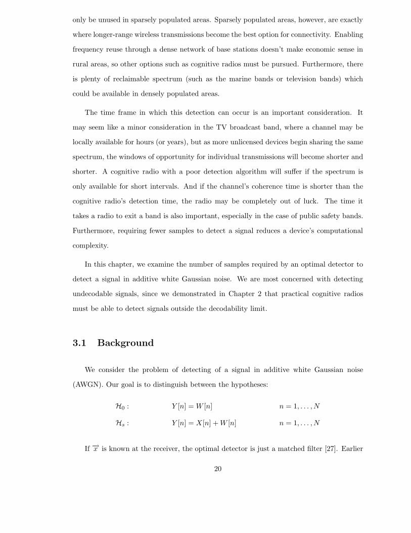
See Fig. 3.1a for the performance curves of this detector.
−60 −50 −40 −30 −20 −10 00
2
4
6
8
10
12
14
SNR (in dB)
log 10
N
Energy DetectorUndecodable BPSKCoherent Detector
BPSK −− Detector Performance
(a) The optimal detector for un-
decodable BPSK requires nearly as
many samples�∼
1SNR2
�for detec-
tion as an energy detector. A coher-
ent detector performs significantly
better�∼
1SNR
�.
−60 −50 −40 −30 −20 −10 00
2
4
6
8
10
12
14
SNR (in dB)
log 10
N
Energy Detector Undecodable BPSKBPSK with Pilot signal Sub−optimal schemeDeterministic BPSK
BPSK −− Detector Performance
(b) Just detecting the weak pilot sig-
nal is nearly optimal at low SNR.
Figure 3.1. Samples (N) required to detect a signal with a predetermined probability of error. With no
pilot signal present, an optimal detector performs only marginally better than an energy detector. If a weak
pilot signal is present, far fewer samples are necessary for detection.
3.3 Detection of zero-mean constellations
3.3.1 Model
We examine the maximum likelihood decision rule for a constellation known to the
receiver, subject to the constraint that the symbols have low energy. We show that the
optimal detector for a zero-mean constellation behaves like a energy detector in the limit
of low SNR. [30] shows the same result for biorthogonal signal constellations.
We assume a constellation of 2LR symbols. Each symbol has dimension L and R is
greater than the channel’s capacity. The transmitter picks a sequence of N (N large)
i.i.d. symbols and transmits it over the channel.
H0 :−→Y [n] =
−→W [n]
Hs :−→Y [n] =
−→X [n] +
−→W [n]
where −→x [n] = −→c i , i ∈ (1, 2LR) and−→W [n] ∼ N (0, σ2IL).The probability that the ith symbol
22

in the constellation, denoted −→c i, is transmitted is Pr(−→c i). We denote the energy in the
ith symbol by Γ(i) = −→c Ti−→c i, and the average symbol energy by Γ =
∑2LR
i=1 Pr(−→c i)
−→c Ti−→c i.
The signal−→Y of lengthN is received, and a maximum likelihood rule is used to determine
whether the signal is purely noise, or whether a symbol was transmitted.
3.3.2 Results
The approximate maximum likelihood decision rule is shown below. (See next section
for derivation.)
N∑
n=1
1
σ2
2LR∑
i=1
Pr(−→c i)−→c T
i
−→Y [n] − Γ
2σ2+
1
8σ4
2LR∑
i=1
Pr(−→c i)(2−→c T
i
−→Y [n] − Γi)
2
Hs
≷H0
0 (3.1)
Assuming low SNR, under what further conditions does our optimal detector reduce to
a energy detector? The bracketed term, like a matched filter, is a linear function of−→Y . If
this term equals zero, the−→Y T−→Y terms, smaller by a factor of SNR, become the dominant
terms.
∑2LR
i=1 Pr(−→c i)
−→c Ti is just the average of the symbol constellation. Therefore, if all the
symbols in our codewords are chosen from zero-mean signal constellations, the optimal
detector at low SNR behaves qualitatively like an energy detector (Fig. 3.2) in its dependence
on SNR.
3.3.3 Analysis
We derive expressions for the probability of receiving−→Y under the H0 and Hs hypothe-
ses:
Pr(−→Y | H0) =
1
(2πσ2)L/2exp
( −1
2σ2
−→Y T−→Y
)
Pr(−→Y | Hs) =
2LR∑
i=1
Pr(−→c i)1
(2πσ2)L/2exp
( −1
2σ2(−→Y −−→c i)
T (−→Y −−→c i)
)
23

−60 −50 −40 −30 −20 −10 010
2
104
106
108
1010
1012
1014
SNR (dB)
log 10
N
Asymmetric Constellation − Detector Performance
Optimal DetectorEnergy Detector
Figure 3.2. Samples (N) required to detect a signal with a predetermined probability of error. For a
zero-mean constellation, the energy detector is nearly optimal.
The independence of the N transmitted symbols results in the maximum likelihood rule:
N∏
n=1
2LR∑
i=1
Pr(−→c i) exp
(1
2σ2(2−→c T
i
−→Y [n] −−→c T
i−→c i)
)
Hs
≷H0
1
We assume 12σ2 (2−→c T
i
−→Y [n]−−→c T
i−→c i) ≪ 1. Using the approximation ex ≈ 1 + x+ x2
2 we
have:
(We assume Γ(i)2σ2 ≪ 1 and 1
σ2
∑Mj=1 yj[ℓ]cj(i) ≪ 1)
N∏
n=1
1 − Γ
2σ2+
1
σ2
2LR∑
i=1
Pr(−→c i)−→c T
i
−→Y [n] +
1
8σ4
2LR∑
i=1
Pr(−→c i)(2−→c T
i
−→Y [n] − Γi)
2
Hs
≷H0
1
(3.2)
We can take the natural logarithm of each side and use ln(1 + x) ≈ x to yield the
decision rule in 3.1.
Independence between symbols is important to the previous result. However, we do not
24

require identical distributions. The same result applies to symbols that are only condition-
ally zero mean, given the rest of the coded symbols.
3.4 Pilot signals and training sequences
We have shown that zero-mean signals are difficult to detect at low SNR. Knowing the
modulation scheme does not help. We can significantly improve the performance of our
detector by transmitting an additional, known pilot signal or training sequence. At high
SNR, an energy detector is nearly optimal [31], but it performs far worse than a coherent
detector at low SNR.
If the transmitter sends a pilot signal simultaneously with its transmissions, we can
design a suboptimal detector which just detects the pilot at low SNR. Coherent detection
via a matched filter results in processing gain and a substantial reduction in the number of
samples required for detection, even for extremely weak pilot signals. Simulations further
show that this scheme is nearly optimal at low SNR, i.e. a secondary receiver can just look
for a pilot signal and ignore the remainder of the transmission. Refer to Fig. 3.1b for the
performance curves in the presence of a pilot signal.
25

Chapter 4
Power control
In previous chapters, we demonstrated that a number of fundamental limitations can
be overcome if the licensed (primary) transmitter transmits a perfectly known pilot signal
or training sequence to aid detection. This pilot signal has the additional benefit of al-
lowing users to measure the local SNR of the primary signal, which can then be used as
a proxy for distance from the primary transmitter. Armed with this information, cogni-
tive radios (secondary users) can approximate their distance from the primary transmitter
and adjust their transmit power accordingly. We assume the secondary users can measure
their local SNR accurately. Due to random channel fluctuations, this may require multiple
measurements [10].
We should note that we use SNR, not SINR, as a metric. Local SNR can be measured
by allowing the primary transmitter’s pilot signal to double as a synchronization signal so
that the secondary transmitters can periodically all fall silent together and measure their
local SNR without interference from other secondaries. Alternatively, SINR could be used
if the interference resulting from other secondary users can be determined.
In this chapter we present an example of a power control rule which allows secondary
users to aggressively increase their transmit powers while still guaranteeing an acceptable
level of aggregate interference at the primary receivers. Of particular concern are the effect
of different propagation path losses for different systems, the effect of multiple cognitive
26

users, and the effect of heterogeneous transmit powers among the cognitive users. We
demonstrate that none of these issues invalidates cognitive radio’s feasibility.
After a brief review of previous work (4.1) and a description of our model (4.2), we
consider a single secondary user sharing spectrum with the primary system. We further
divide the single secondary user regime into two subcases. We can think of the secondary
users as licensed users constrained to a specific power. This could happen if two distinct
property rights were auctioned off for a particular frequency band. For example, company
A could purchase the right to transmit up to 10 kW on the 800-900 MHz band anywhere
in the US. while company B could purchase the right to transmit up to 1 kW on the same
band but only when A is not using it. On the other hand, it seems reasonable to allow a
secondary user to use more power if he is further from the primary system.
We examine both these cases in section 4.5, followed by the effects of shadowing/fading
in section 4.6. In section 4.7, we extend our analysis to multiple secondary users. We con-
sider first the case in which all the secondary users are bound by the same power constraint.
Finally, in section 4.8, we allow the secondary users to be heterogeneous in nature and to
increase their transmit power with distance from the primary system. This final viewpoint
more closely aligns with the traditional view of cognitive radio [12]. After first allowing the
secondary users to increase their power without bound, we observe that practical radios
will have a minimum detectable SNR [24], so failure to detect a signal means only that the
SNR has fallen below some threshold. This caps a cognitive radio’s transmit power and is
explored in section 4.9.
4.1 Related work
The idea that interference is local and frequencies may be reused is not new. Spatial
considerations for frequency reuse have been studied extensively in cellular systems [32],
[33]. However, these systems differ from the cognitive radio case in a number of significant
ways.
Most of the interference in a cellular system is within-system interference, caused by
27

devices the spectrum owner designs. It can therefore be tightly controlled, both in terms of
its power and its spectral characteristics.
Cognitive radios, on the other hand, do not just cause out-of-cell interference, they
cause out-of-system interference. This interference comes from a sea of heterogeneous de-
vices with varying powers, duty cycles, and even propagation path losses. Previous research
into frequency reuse in cellular networks has made the reasonable assumption of user homo-
geneity [34]–[36]. When considering the interaction between cellular telephones or 802.11
access points, one can assume that in-cell and out-of-cell transmitters use the same power
control rules and experience the same propagation path loss.
In the case of cognitive radios, however, these assumptions do not hold. Low-powered
cognitive radios may be sharing spectrum with a tall television transmitter. We expect the
cognitive radios will be operating at ground level and hence will experience faster signal
attenuation [37].
This sea of heterogeneous secondary devices must be able to guarantee service to primary
users who are already near the limit of decodability in the no outside-interference case. Cell
planners, designing their cell sizes to guarantee an acceptable level of interference, often
have the additional advantage of a network of base stations whose locations are fixed and
known. For (potentially mobile) cognitive radios, which might lack any sort of regulated
infrastructure, we will use locally measured SNR in place of distance.
4.2 Model
In our model, we assume a band already potentially assigned to a single-transmitter
system. We are particularly interested in long-range primary transmissions such as tele-
vision, but for the sake of comparison we also present examples involving a shorter-range
primary such as a 802.11 wireless access point. Within some protected radius of the primary
transmitter, all unshadowed primary receivers must be guaranteed reception, even when the
cognitive radios are operating. All transmissions are assumed to be omnidirectional.
28

In Chapter 2 we showed that secondary users must be able to coherently detect a known
pilot signal or training sequence from the primary transmitter. If a training sequence is
transmitted as part of the primary transmission, its SNR will be the same as the SNR
of the data portion of the transmission. We will make this assumption throughout this
chapter.
However, the pilot signal case is more complicated. First of all, the pilot signal may
be significantly weaker than the primary’s data signal, perhaps 20 dB or more down. This
will have the same result as insurmoutable shadowing (section 4.6), forcing secondary users
to detect a 20 dB weaker signal. This effect will be clearly seen if the pilot is sent in a
separate frequency band or time slot from the primary transmission. However, if the pilot
signal and the primary data signal are sent in the same band, there will be a non-linear
effect on the pilot signal’s SNR due to interference from the data signal. Near the primary
transmitter, the data signal will dominate the noise experienced by pilot signal detectors,
making pilot signal SNR a poor proxy for distance. However, in this high SNR regime,
the optimal detector (Chapter 3) is a radiometer, not a coherent detector of a weak signal.
The SNR of the entire primary transmission, not just the SNR of the pilot signal, would
therefore be an appropriate proxy for distance. For secondary users far from the primary
transmitter, especially in the middle of nowhere, the noise from the primary data signal will
be significantly attenuated and be much weaker than the ambient noise. This non-linear
effect will be addressed in future work.
4.3 SNR as a proxy for distance
The primary system has a minimum required SINR to successfully decode at its target
rate R. In the absence of interference, this γdec occurs at a radius rdec from the transmitter.
The idea is to guarantee service to primary users within some protected radius (rp) by
defining an additional “no-talk radius” (rn) within which secondary users must be quiet
(Figure 4.1). At distances from the primary transmitter greater than rn, secondary users
might be allowed to transmit. Ideally, these “no-talk regions” would be centered on each
29

of the primary system’s receivers, but we assume that the cognitive radios have no way of
knowing these locations.
If there is uncertainty in the noise power, then we can choose rdec first and set σ2 to
the maximum tolerable noise at that radius. If the noise power crosses this threshold with
the cognitive radios transmitting, then protected users at rp could experience an outage.
However, this noise event would cause an outage for primary users at rdec even without the
cognitive radios. We also assume that this σ2 is preprogrammed into the cognitive radio, so
it does not need to be continually estimated. Designing radios to compensate for changing
noise floors is a topic for future research.
Since we are using locally measured SNR as a proxy for distance, it is convenient to
represent rdec, rp, and rn in terms of the SNR in dB measured at those points. We assume
we are coherently detecting a known signal of the same power as the primary data signal,
and that ambient noise is the only source of noise, as in the case of a training sequence. In
this case, locally measured SNR can be used straightforwardly as a proxy for distance from
the primary transmitter. However, if a primary receiver is a TV antenna on a roof, it might
measure an SNR of 0 dB at one location, while a cognitive radio on the ground at the same
location might measure -10 dB. Therefore we must specify who is measuring the SNR at
each distance. We consider γdec and γp to be measured by a primary receiver, while γn is
by a secondary transmitter. Denoting the power of the primary transmitter as P1, and the
power of the noise at the primary receiver σ2, we define:
∆ , 10 log
(P1
σ2
)− γdec
µ , γp − γdec
ν , γdec − γn
For example, if the minimum decodable SNR for the primary receiver is 10 dB and a
secondary transmitter measures an SNR of -5 dB at rn, then ν = 15. We also define ψ to
be the margin between γdec and the local SNR measured by a particular secondary user.
30

ψ∆rdecrp rn
νµ
Figure 4.1. SNR margins can be used as a proxy for distance
As in [38], we represent the propagation-related power attenuation between two users
a distance r apart as a function g(r) defined on [0,∞]. We require g(r) to be continuous
with 0 < g(r) ≤ C · r−2−ǫ (free-space propagation loss) for some C > 0, ǫ > 0. We allow
different gain functions g11(r), the propagation path loss between the primary transmitter
and primary receiver, g12(r), between the primary transmitter and secondary receiver, and
g21(r), between the secondary transmitter and primary receiver. Throughout this paper,
our examples will be g11(r) = g12(r) = r−α1 and g21(r) = r−α2 .
For example, for the gain function g11(r) = r−3.5, ∆ = 165 corresponds to a transmitter
with about a 52 km range:
∆ = 165 = 10 log
(P1
σ2
)− 10 log
(P1r
−4dec
σ2
)
rdec = 10165
3.5·10 ≈ 51800 (4.1)
Further, consider µ = 1dB and ν = 0.01dB as potential operating margins. In this case,
rdec − rp ≈ 3300m, while rn − rdec ≈ 34m. Because of the large protected radius, very
small increments in dB correspond to large physical distances. This is important, because it
means that the necessary operating margins can be quite small (Table 4.1). Unless otherwise
specified, we will assume µ = 1 for our plots.
Our assumption of a 52 km decodability radius is actually quite conservative. KRON-
TV in San Francisco has an effective service radius of approximately 120 km [39], [40].
Furthermore, attenuation is slower than r−4, which causes small SNR margins to correspond
to even greater distances (Table 4.2). The magnitude of these differences makes it clear that
an accurate model will be essential when designing practical cognitive systems.
31
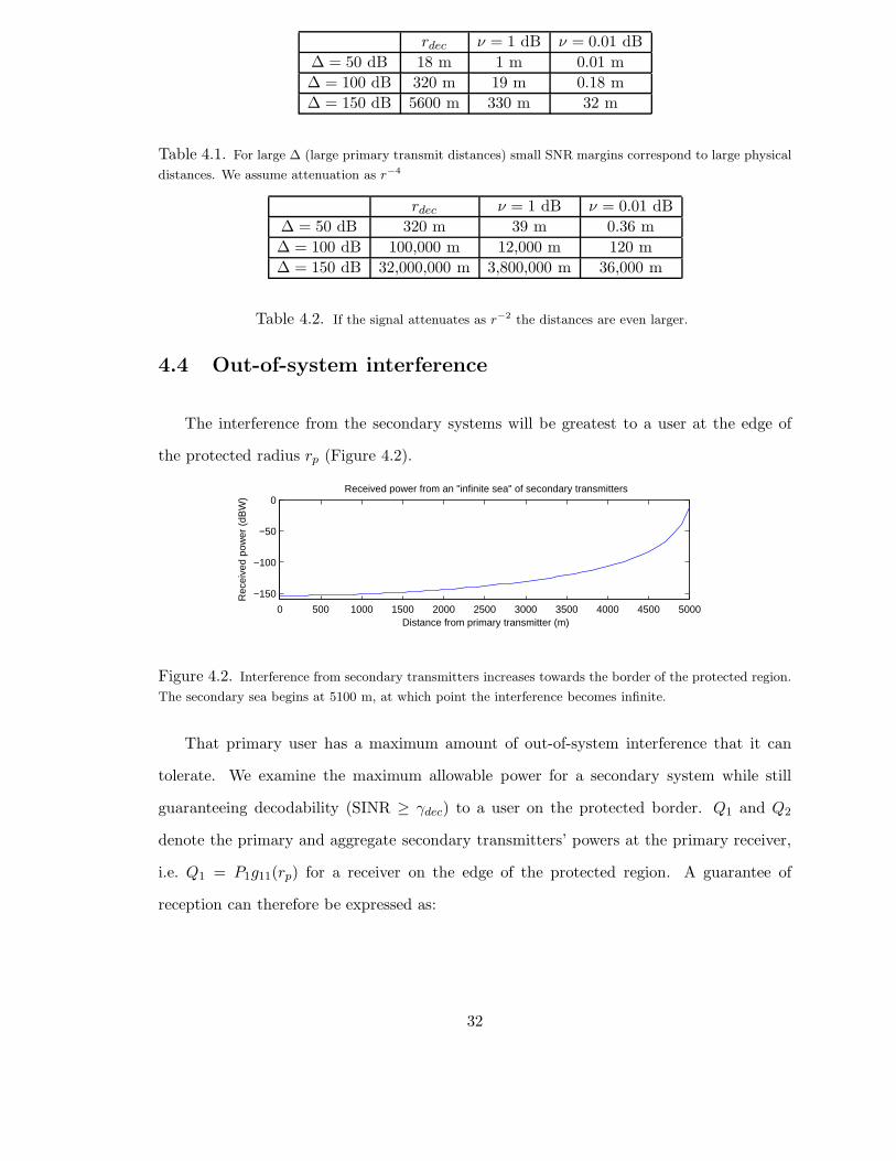
rdec ν = 1 dB ν = 0.01 dB
∆ = 50 dB 18 m 1 m 0.01 m
∆ = 100 dB 320 m 19 m 0.18 m
∆ = 150 dB 5600 m 330 m 32 m
Table 4.1. For large ∆ (large primary transmit distances) small SNR margins correspond to large physical
distances. We assume attenuation as r−4
rdec ν = 1 dB ν = 0.01 dB
∆ = 50 dB 320 m 39 m 0.36 m
∆ = 100 dB 100,000 m 12,000 m 120 m
∆ = 150 dB 32,000,000 m 3,800,000 m 36,000 m
Table 4.2. If the signal attenuates as r−2 the distances are even larger.
4.4 Out-of-system interference
The interference from the secondary systems will be greatest to a user at the edge of
the protected radius rp (Figure 4.2).
0 500 1000 1500 2000 2500 3000 3500 4000 4500 5000
−150
−100
−50
0Received power from an "infinite sea" of secondary transmitters
Distance from primary transmitter (m)
Rec
eive
d po
wer
(dB
W)
Figure 4.2. Interference from secondary transmitters increases towards the border of the protected region.
The secondary sea begins at 5100 m, at which point the interference becomes infinite.
That primary user has a maximum amount of out-of-system interference that it can
tolerate. We examine the maximum allowable power for a secondary system while still
guaranteeing decodability (SINR ≥ γdec) to a user on the protected border. Q1 and Q2
denote the primary and aggregate secondary transmitters’ powers at the primary receiver,
i.e. Q1 = P1g11(rp) for a receiver on the edge of the protected region. A guarantee of
reception can therefore be expressed as:
32

Q1
Q2 + σ2≥ SINRdec = 10
γdec10
Q2 ≤ Q110− γdec
10 − σ2 (4.2)
We can express Q1 on the protected border in terms of SNR:
log
(Q1
σ2
)= γdec + µ
Q1 = σ210γdec+µ
10 (4.3)
Substituting into equation (4.2), we see that the secondary system must guarantee:
Q2 ≤ (10µ10 − 1)σ2 (4.4)
This is a fundamental constraint for any secondary system.
4.5 Single secondary transmitter
A one-size-fits-all power constraint must consider a primary receiver and secondary
transmitter as close as possible, with the primary on the edge of the protected zone and the
secondary on the edge of the no-talk zone. (4.4) implies:
P2g21(rn − rp) ≤ (10µ10 − 1)σ2
P2 ≤ (10µ10 − 1)σ2(g21(rn − rp))
−1 (4.5)
A more interesting case occurs when the single secondary transmitter is allowed to vary
its power depending on its proximity to the protected region. We simply replace the worst
case distance rn in equation (4.5) by the secondary’s actual distance r2 from the primary
transmitter. We observe that this new power schedule is strictly better than the “one-size-
fits all” power limit because a secondary user on the edge of the no-talk region is now a
33

worst case scenario. Since these distances are not known to the cognitive radio, we perform
our calculations in terms of SNR.
First, we write rp, the protected radius, in terms of SNR.
10 log
(P1
σ2
)− 10 log
(P1g11(rp)
σ2
)= ∆ − µ
g11(rp) = 10−∆+µ
10
rp = g−111 (10
−∆+µ10 ) (4.6)
Next, we solve for the distance r2 of the secondary transmitter, in terms of his local
SNR.
10 log
(P1
σ2
)− 10 log
(P1g12(r2)
σ2
)= ∆ + ψ
g12(r2) = 10−∆−ψ
10
r2 = g−112 (10
−∆−ψ10 ) (4.7)
Equations (4.6) and (4.7) let us write (4.5), the maximum allowable power for a sec-
ondary transmitter, in SNR terms.
P2
σ2≤ (10
µ10 − 1)(g12(r2 − rp))
−1
=(10
µ10 − 1)
(g21(g−112 (10
−∆−ψ10 ) − g−1
11 (10−∆+µ
10 )))(4.8)
For our example gain functions g11(r) = g12(r) = r−α1 and g21(r) = r−α2 this gives us:
10 log
(P2
σ2
)≤ α2
αp∆ + 10 log(10
µ10 − 1)
+ 10α2 log
((10
ψ10
) 1αp −
(10−
µ10
) 1αp
)(4.9)
The first term describes how aggressively the primary user is transmitting, i.e. how far
a user can travel from the primary transmitter and still decode the signal. Increasing the
primary transmitter’s rate without increasing its power decreases ∆ and therefore requires
the secondary transmitter to quiet down. The second term represents how tolerant the
34

protected primary receivers are to interference. The final term represents how far the sec-
ondary transmitter is from the protected receivers. Also note that if ψ = −µ the secondary
transmitter is in the protected region and must be silent.
Figure 4.3 shows the effects of the margin ∆ between the primary transmitter and the
decodability radius, and also the margin µ between the protected radius and the decodbility
radius. We observe a few interesting effects.
First, assuming the cognitive radios wish to transmit at −10 dbW, a small ∆ presents a
problem (Figure 4.3a,b). This requires a large margin ψ (far in excess of 30 dB). Secondary
users must therefore be far more sensitive than the primary users.
For small µ (Figure 4.3a,c), the maximum allowable power for the secondary transmitter
jumps from zero to possibly health-endangering levels as soon as the secondary transmitter is
outside the protected radius. If the secondary users are low powered devices then they only
need to know when they are slightly outside the protected region. Therefore, the cognitive
radio does not need to be significantly more sensitive than the users of the primary system,
which are capable of receiving a signal all the way out to the decodability radius. Because
the increase in allowable power is so rapid, any sensitivity beyond that hardly buys the
secondary user anything.
A larger margin µ allows secondary transmitters to transmit geographically much closer
to the protected region. Not only does this allow much greater reuse of physical space, but
more powerful secondary transmitters (an 802.11g access point is ≈ −10 dBW) can also
have far less sensitive detectors (Figure 4.3d). This tradeoff cannot be resolved technically;
a policy decision needs to be made.
The figures also illustrate the effect of different decay rates α1 and α2. If α2 > α1,
i.e. the secondary user’s transmissions attenuate faster with distance than the primary
transmissions do, we see the secondary user can use more power than he could if both
systems experienced the same path loss. This is likely to be the case, for example, if the
primary transmitter is a tall TV antenna while the secondary users are located on the
ground. The significance of the case in which α1 > α2 will become apparent in section 4.7.
35

4.6 Single secondary transmitter with shadowing/fading
We now extend our model to the case in which the secondary transmitter may lie in a
shadow (signal loss of β dB) with respect to the primary signal. A secondary transmitter
must now measure a margin of ν + β to be certain that he is outside the no-talk zone.
Adjusting equation (4.9) to account for shadowing, we get:
P2
σ2≤ (10
µ10 − 1)
(g21(g−112 (10
−∆−(ψ−β)10 ) − g−1
11 (10−∆+µ
10 )))(4.10)
Because a secondary transmitter can never assume it is unshadowed, we see that shad-
owing results in a pure shift of the curve in Figure 4.4. As an aside, we are assuming the
gain functions are deterministic, but since we are using local SNR as our distance metric,
this result can be extended to a dynamically fading channel by treating a multipath fade
as additional shadowing [41].
However, one distinction is worth noting. While multipath fading can be nearly inde-
pendent between nearby users, shadowing is likely to be highly correlated. This is actually
a problem with our model. We have assumed there is no “local continuity” to shadowing,
i.e. that a shadowed secondary user could sit right next to an unshadowed primary user.
In practical environments, however, if a user is deeply shadowed, other users within a few
meters are most likely also deeply shadowed. Since we are only interested in protecting
primary users who can decode a signal in the first place, a secondary user shadowed deeply
enough that he cannot decode the primary signal could predict that he is likely to be a few
meters away from any primary receiver.
This knowledge could potentially confer a benefit (in addition to those discussed in
Chapter 2) on a secondary user with the ability to determine whether he is shadowed with
respect to the primary transmitter. More importantly, however, is that 10 dB of shadowing
will no longer result in exactly a 10 dB shift of the allowable power graph. A shadowed
secondary user transmitting inside the protected region has less potential to cause severe
interference if local continuity implies an implicit buffer zone around him.
For the sake of simplicity, we ignore this benefit in our model. Considering it would
36
greatly complicate things because our model treats multipath fading and shadowing the
same way. However, multipath has no local continuity. A secondary user in a deep multipath
fade cannot assume that the users around him are similarly faded.
Multipath fading and shadowing are therefore not interchangeable. The locally contin-
uous nature of shadowing may have important ramifications for cognitive radio protocols.
Among other considerations, future techniques to improve detection (such as cooperation
among cognitive radios) may be more effective against multipath fading than against shad-
owing [10].
4.7 Multiple licensed secondary transmitters
Suppose now that we are no longer limited to a single interferer. Outside of the no-talk
circle of radius rn, we assume there exists a sea of secondary transmitters, each with power
P2. We further assume that there is a limit to how densely these transmitters are packed.
Each secondary transmitter uniquely occupies a footprint of area A, so this “secondary sea”
has a power density D = P2A . Integrating over this sea gives the aggregate power of the
secondary transmissions at a primary receiver on the edge of the protected region.
As in the case of the single licensed transmitter, we assume a constant power density
outside the no-talk zone. Later, in section 4.8, we will consider the case in which secondary
users are allowed to increase the power of their transmissions as they venture further from
the protected region.
We first assume that the secondary transmission power decays as g21(r) = r−α2, α2 > 2.
We also assume rp ≫ rn−rp, the distance between the primary receivers and the secondary
transmitters. For a primary receiver on the edge of the protected region, the “coast” of the
secondary sea can be approximated by a line a distance of rn − rp away. We examine the
quality of this approximation in a later calculation (4.14).
Q2 =
∫ π2
−π2
∫ ∞
rn−rpcos(θ)
Dr−α2 r dr dθ (4.11)
37

=D
−α2 + 2
∫ π2
−π2
[r−α2+2
]∞rn−rpcos θ
dθ
=D · (rn − rp)
−α2+2
α2 − 2
∫ π2
−π2
(cos θ)α2−2 dθ
= D ·K(α2) · (rn − rp)−α2+2 (4.12)
where K(α2) =
R π2
−π2
(cos θ)α2−2 dθ
α2−2 .
For α2 = 6, K(α2) = 14
3!!4!!π ≈ 0.295.
The entire sea of secondary transmitters behaves like a single transmitter of power
D · K(α2), located a distance rn − rp away (i.e. at the coast of the sea), but with a new
decay exponent of −α2 + 2.
For small rn−rp, the majority of the interference comes from the few secondaries closest
to the vulnerable primary receiver. As the secondary sea moves further away, more of the
sea becomes “visible” to the receiver, explaining why the decay is now as r−α2+2. The effect
of increasing the secondary decay exponent by two is illustrated in Figure 4.3.
This approximation, however, understates the interference caused by the secondary sea
in Figure 4.5a. We can upperbound the interference by considering the case where a primary
receiver is completely surrounded by a secondary sea a distance rn − rp away. Using our
generalized gain functions:
Q2 =
∫ π
−π
∫ ∞
rn−rp
D · g21(r) r dr dθ
= D
∫ π
−π[rg21(r) − g21(r)]
∞rn−rp dθ
where g21(r) = ddr g21(r) = d2
dr2 g21(r). Since g(r) ≤ C ·r−2−ǫ, limr→∞(rg21(r)− g21(r)) =
0 and it follows:
Q2 = D · 2π · (g21(rn − rp) − (rn − rp)g21(rn − rp)) (4.13)
Specifically, for our example gain functions, we have
Q2 = D · 2π
α2 − 2· (rn − rp)
−α2+2 (4.14)
38

Again, this bound claims that the sea behaves like a single transmitter of power located
a distance rn − rp away but with a new decay exponent −α2 + 2.
Figure 4.6 shows that the straight line approximation is quite good. Having multiple
secondary users does change the decay rate of the aggregate interference, but we have
already seen that the limits on the allowable transmit power can still be quite generous
for large ∆ primaries (TV). For systems (802.11) with smaller ∆, the change in decay rate
could be compensated for with either a larger SNR margin ν between the protected radius
and the no-talk zone, or a larger SNR margin µ to the decodability limit.
4.8 Multiple dynamic secondary transmitters
We now consider the case in which secondary users are allowed to increase the power
of their transmissions as they move further from the protected region. Clearly, the rule we
pick to govern D(r) will determine the impact of the secondary sea on the primary receivers.
Noting that 1g21(r) is an increasing function, we assume the power density to be governed
by a rule of the form:
D(r) = D0(ρ)1
g21(r)r−ρ (4.15)
where ρ is a constant that determines how aggressively the power density D(r) should
increase with r. This rule can be expressed in terms of local SNR, ψ, in (4.20).
To determine the aggregate interference at a primary receiver on the edge of the pro-
tected region, we use the straight line approximation for the coast of the sea. For a particular
ρ:
Q2 =
∫ π2
−π2
∫ ∞
rn−rpcos(θ)
D(r)g21(r) r dr dθ (4.16)
=D0(ρ)
−ρ+ 2
∫ π2
−π2
[r−ρ+2
]∞rn−rp
cos θdθ
39
If ρ > 2, i.e. D(r2) grows sufficiently slower than g21(r2), then the integral converges.
=D0(ρ)
∫ π2
−π2(cos θ)ρ−2 dθ
ρ− 2(rn − rp)
−ρ+2
= K(ρ) ·D0(ρ) · (rn − rp)−ρ+2 (4.17)
With this particular rule for the power density, the sea of secondary transmitters behaves
like a single transmitter located rn − rp from the protected radius, with power K(ρ) ·D0(ρ)
and gain function g21(r) = r−ρ+2. We can plug our expression straight into (4.8) to get an
bound on D0(ρ).
D0(ρ) ≤ σ2 (10µ10 − 1)
K(ρ) · (g−112 (10
−∆−ν10 ) − g−1
11 (10−∆+µ
10 ))−ρ+2(4.18)
From (4.6) and (4.7) we can express r in terms of SNR:
r = r2 − rp = g−112 (10
−∆−ψ10 ) − g−1
11 (10−∆+µ
10 ) (4.19)
With (4.18) and (4.19) we can express (4.15) as a function of ψ:
D(ψ) = σ2
((10
µ10 − 1)
K(ρ) · (g−112 (10
−∆−ν10 ) − g−1
11 (10−∆+µ
10 ))−ρ+2
)
((g−1
12 (10−∆−ψ
10 ) − g−111 (10
−∆+µ10 ))−ρ
g21(g−112 (10
−∆−ψ10 ) − g−1
11 (10−∆+µ
10 ))
)(4.20)
This equation gives the the allowable power density for secondary transmitters as a
function of distance, measured in dB, from the protected region. The more aggressively
the secondary transmitters increase their power with distance, the quieter the secondary
transmitters near the primary system must become. An example of the allowable density for
secondary users interfering with a digital TV station (∆ = 165) is depicted in Figure 4.7a.
This particular plot uses a margin of µ = 1, so there must be a margin of at least 11
dB (compensating for 10 dB of possible shadowing) between the protected radius and the
secondary users before they are allowed to transmit at all. Figure 4.7b shows that if the
40

margins are too small (i.e. secondary users are allowed to transmit too close to the protected
receivers) secondary users everywhere will be crippled by the power density limits.
The primary receivers have a certain margin µ of tolerable interference that through
policy decisions can be allocated to users at different distances. The more aggressively
(smaller ρ) the secondary transmitters increase their power with distance, the quieter the
secondary transmitters near the primary system must become.
4.9 Minimum detectable SNR
In the preceding sections we mentioned an implicit cap on the transmit powers of the
secondary users. Many factors contribute to this upper limit on power, including safety or
hardware limitations. It is also affected by a radio’s sensitivity:
As a secondary transmitter moves away from the protected radius, its allowable power
increases exponentially. At some distance rmax, however, the local SNR at the secondary
transmitter will drop below its minimum detectable SNR, γmin [23]. From this point out-
wards, the secondary receiver cannot assume it is more than a distance rmax away from the
transmitter, no matter what its actual distance. As a result, there is an absolute cap on the
secondary transmit power. This in turn changes the aggregate interference at a primary
transmitter on the border of the protected region.
Q2 =
∫ π2
−π2
∫ rmax
rn−rpcos(θ)
D(r)g21(r) r dr dθ
+
∫ π2
−π2
∫ ∞
rmax
D(rmax)g21(r) r dr dθ (4.21)
=D0
−ρ+ 2
∫ π2
−π2
[r−ρ+2
]rmaxrn−rp
cos θ
dθ
+D(rmax)
−ρ+ 2
∫ π2
−π2
[rg21(r) − g21(r)]∞rmax
dθ
= K(ρ) ·D0 · (rn − rp)−ρ+2 − D0
ρ− 2πrmax
−ρ+2
+D(rmax)
ρ− 2π [g21(rmax) − rmaxg21(rmax)] (4.22)
41
We can express rmax in terms of γmin.
γmin = 10 log
(P1g12(rmax)
σ2
)− β
rmax = g−112
(σ2
P110
γmin+β
10
)(4.23)
We can use (4.22), (4.23), and (4.4) to find a bound on D0. Alternatively, we could
solve this expression for γmin. If a manufacturer wanted to build cognitive radios that avoid
interfering with legacy systems, γmin represents how sensitive his radios’ detection hardware
must be.
42

0 5 10 15 20 25 30−200
−150
−100
−50
0
50
100
150Maximum power for secondary transmitter, ∆=35 (WiFi)
SNR margin ψ at secondary receiver (dB)
Max
sec
onda
ry p
ower
(dB
W)
(a) ∆ = 35 (rdec = 10m), µ=0.1
0 5 10 15 20 25 30−200
−150
−100
−50
0
50
100
150Maximum power for secondary transmitter, ∆=35 (WiFi)
SNR margin ψ at secondary receiver (dB)
Max
sec
onda
ry p
ower
(dB
W)
(b) ∆ = 35 (rdec = 10m), µ=1.0
0 5 10 15 20 25 30−200
−150
−100
−50
0
50
100
150Maximum power for secondary transmitter, ∆=165 (Digital TV)
SNR margin ψ at secondary receiver (dB)
Max
sec
onda
ry p
ower
(dB
W)
(c) ∆ = 165 (rdec = 52km), µ=0.1
0 5 10 15 20 25 30−200
−150
−100
−50
0
50
100
150Maximum power for secondary transmitter, ∆=165 (Digital TV)
SNR margin ψ at secondary receiver (dB)
Max
sec
onda
ry p
ower
(dB
W)
(d) ∆ = 165 (rdec = 52km), µ=1.0
· · · · · · · · · α1 = 3.5, α2 = 5
α1 = 3.5, α2 = 3.5
− − − α1 = 5, α2 = 3.5
Figure 4.3. Maximum power for a secondary transmitter vs. dB beyond rdec. ∆ measures the primary
signal attenuation from the transmitter to the decodability radius. For reference, we also give the distance
to the decodability radius, assuming attentuation as r−3.5 (i.e. α1 = 3.5).
43

0 5 10 15 20 25 30−50
−40
−30
−20
−10
0
10
20
30
40
50Maximum power for secondary transmitter
SNR margin ψ at secondary receiver (dB)
Max
sec
onda
ry p
ower
(dB
W)
No shadowing10 dB shadowing
10 dB
Figure 4.4. The possibility of 10 dB of shadowing results in a 10 dB shift of the required SNR margin
(eqn. 4.10).
��������������������������������������������������������������������������������������������������������������������������������������������������������������������������������������������������������������������������������������������������������������������������������������������������������������������������������������������������������������������������������������������������������������������������������������������������������������������������������������������������������������������������������������������������������������������������������������������������������������������������������������������������������������������������������������������������������������������������������������������������������������������������������������������������������������������������������������������������������������������������������������������������������������������������������������������������������������������������������������������������������������������������������������������������������������������������������������������������������������������������������������������������������������������������������������������������������������������������������������������������������������������������������������������������������������������������������������������������������������������������������������������������������������������������������������������������������������������������������������������������������������������������������������������������������������������������������������������������������������������������������������������������������������������������������������������������������������������������������������������������������������������������������������������������������������������������������������������������������������������������������������������������������������������������������������������������������������������������������������������������������������������������������������������������������������������������������������������������������������������������������������������������������������������������������������������������������������������������������������������������������������������������������������������������������������������������������������������������������������������������������������������������������������������������������������������������������������������������������������������������������������
��������������������������������������������������������������������������������������������������������������������������������������������������������������������������������������������������������������������������������������������������������������������������������������������������������������������������������������������������������������������������������������������������������������������������������������������������������������������������������������������������������������������������������������������������������������������������������������������������������������������������������������������������������������������������������������������������������������������������������������������������������������������������������������������������������������������������������������������������������������������������������������������������������������������������������������������������������������������������������������������������������������������������������������������������������������������������������������������������������������������������������������������������������������������������������������������������������������������������������������������������������������������������������������������������������������������������������������������������������������������������������������������������������������������������������������������������������������������������������������������������������������������������������������������������������������������������������������������������������������������������������������������������������������������������������������������������������������������������������������������������������������������������������������������������������������������������������������������������������������������������������������������������������������������������������������������������������������������������������������������������������������������������������������������������������������������������������������������������������������������������������������������������������������������������������������������������������������������������������������������������������������������������������������������������������������������������������������������������������������������������������������������������������������������������������������������������������������������������������������������������������������
(a) Secondary sea (b) Sea detail
Figure 4.5. A circular coast looks like a straight line to primary users near the edge of the protected
radius.
44

0 5 10 15 20−60
−50
−40
−30
−20
−10
0
10
20Aggregate secondary power at primary receiver vs. distance to sea
Distance to secondary sea (m)
Agg
rega
te s
econ
dary
pow
er (
dBW
)
Upper boundTrue aggregate powerStraight line coast
Figure 4.6. The upper (eqn. 4.14) and lower (eqn. 4.12) bounds have the same decay exponent. Approx-
imating the coast of the secondary sea with a straight line is accurate to within a constant.
10 12 14 16 18 20−70
−60
−50
−40
−30
−20
−10
SNR margin to secondary transmitter (ψ dB)
Max
imum
allo
wab
le p
ower
den
sity
(dB
W/m
2 )
Maximum allowable secondary power density (∆=165, µ=1)
r2, ν=3
r1, ν=3
r0, ν=3
r2, ν=1
r1, ν=1
r0, ν=1
r2, ν=0.1
r1, ν=0.1
r0, ν=0.1
(a) ∆ = 50, µ = 1
10 12 14 16 18 20−70
−60
−50
−40
−30
−20
−10
SNR margin to secondary transmitter (ψ dB)
Max
imum
allo
wab
le p
ower
den
sity
(dB
W/m
2 )
Maximum allowable secondary power density (∆=165, µ=0.1)
r2, ν=3
r1, ν=3
r0, ν=3
r2, ν=1
r1, ν=1
r0, ν=1
r2, ν=0.1
r1, ν=0.1
r0, ν=0.1
(b) ∆ = 50, µ = 0.1
Figure 4.7. (a) More aggressive power control rules (eqn. 4.20) require a lower density of secondary
transmissions near the protected region. (b) If the margins are too small, secondary users are excessively
constrained.
45
Chapter 5
Conclusion
The FCC’s current “exclusive-use” licensing process has resulted in a serious discrep-
ancy between spectrum allocation and usage. New technologies present the hope that this
underutilized spectrum can be scavenged, but no major policy changes can be expected
without a guarantee of non-interference to legacy/protected users.
We have considered the case of cognitive radio, wireless devices that adjust their trans-
missions in response to their environment. By dynamically adjusting their transmissions
to only use underutilized bands, cognitive radios could be the key to scavenging the under-
utilized spectrum in an area. However, they must be able to do so while minimizing the
interference they cause existing users.
We focused on the case of a single legacy transmitter whose spectrum is shared with
cognitive radios. Starting from first principles, we examined the fundamental restrictions
on cognitive radios necessary to guarantee service to legacy/priority users. Examining
the tradeoffs between secondary user power, available space for secondary operation, and
interference protection for the primary receivers shows that it is imperative for practical
cognitive radios to be able to detect undecodable signals. The “don’t transmit if you
can decode a signal” rule is inadequate for practical systems. Using it anyway could cause
interference in a huge percentage of the primary system’s original service area. This penalty
occurs as a result of shadowing and multipath. Users who can determine whether or not
46

they are shadowed with respect to the primary transmitters or receivers will be able to
reclaim a significant amount of otherwise unusable real estate. The benefits of pinpointing
the locations of the primary receivers are far less.
We pointed out that guaranteeing non-interference begins fundamentally with a de-
tection problem. Calculations and simulations have shown that a potentially prohibitive
number of samples are required to detect symbols from a zero-mean constellation. Detection
is greatly enhanced if a coherently-detectable pilot signal or training sequence is present in
the primary user’s transmission.
To guarantee non-interference to protected receivers, cognitive radios must adjust their
power levels based on their potential proximity to the receiver. The local SNR of the
primary signal provides a viable metric for an effective power control rule. We examined
the maximum transmit power allowed for secondary users under a “one-size-fits-all” power
constraint and under a “flexibly-licensed” constraint that allows users to increase their
transmissions with distance from the primary system.
The aggregate interference caused by multiple cognitive radios slows the effective decay
rate of the interference. However, examining the effects of heterogeneous propagation path
loss functions proves that this does not preclude the possibility of practical cognitive radio
systems. Adequate sensitivity is the fundamental requirement for a successful cognitive
radio. Where shadowing is possible, cognitive radios must compensate by detecting lower
SNR signals. We proved the fundamental constraint on a cognitive radio’s transmit power
is the minimum SNR it can detect and explored the effect of this power cap.
Cognitive radio is an exciting technology that promises to increase the efficiency of our
current spectrum usage. In this thesis, we have answered some of the fundamental questions
that must be addressed before the FCC will consider allowing cognitive devices into more
frequency bands. There are still more questions to be answered, however. How will multiple
primary transmitters affect the local SNR metric? Can useful secondary systems be built
that conform to the necessary power controls? How can we detect and punish users who
47

violate protocols? These questions must be answered before cognitive radio can become a
reality.
48
References
[1] NTIA, “US frequency allocation chart,” 2003. [Online]. Available: http://www.ntia.doc.gov/osmhome/allochrt.html
[2] R. W. Broderson, A. Wolisz, D. Cabric, S. M. Mishra, and D. Willkomm. (2004) White paper:CORVUS: A cognitive radio approach for usage of virtual unlicensed spectrum. [Online]. Available:http://bwrc.eecs.berkeley.edu/Research/MCMA/CR White paper final1.pdf
[3] E. Kwerel and J. Williams. (2002) A proposal for a rapid transition to market allocation of spectrum.[Online]. Available: http://hraunfoss.fcc.gov/edocs public/attachmatch/DOC-228552A1.pdf
[4] G. Faulhaber and D. Farber, “Spectrum management: Property rights, markets, and thecommons,” in Telecommunications Policy Research Conference Proceedings, 2003. [Online]. Available:http://rider.wharton.upenn.edu/∼faulhabe/SPECTRUM MANAGEMENTv51.pdf
[5] FCC, “FCC 00-401,” Dec. 2000. [Online]. Available: http://www.fcc.gov/Bureaus/EngineeringTechnology/Orders/2000/fcc00401.pdf
[6] Y. Benkler, “Overcoming agoraphobia: Building the commons of the digitally networked environment,”Harvard Journal of Law & Technology, vol. 11, pp. 287–400, Winter 1998.
[7] New America, et al., “Technical reply,” Jan. 2005. [Online]. Available: http://www.newamerica.net/Download Docs/pdfs/Doc File 2202 1.pdf
[8] FCC, “FCC 98-208,” Sept. 1998. [Online]. Available: http://www.fcc.gov/Bureaus/EngineeringTechnology/Orders/2000/fcc00401.pdf
[9] J. H. Snider and N. Holmes, illus., The Cartoon Guide to Federal Spectrum Policy. Washington,D.C: New America Foundation, Apr. 2004. [Online]. Available: http://www.newamerica.net/Download Docs/pdfs/Pub File 1555 1.pdf
[10] X. Liu and Sai Shankar N, “Sensing-based opportunistic channel access,” Submitted to ACM Mobile
Networks and Applications Journal, Mar. 2005.
[11] I. J. Mitola, “Software radios: Survey, critical evaluation and future directions,” IEEE Aerospace and
Electronics Systems Magazine, vol. 8, pp. 25–36, Apr. 1993.
[12] FCC, “FCC 03-322,” Dec. 2003. [Online]. Available: http://hraunfoss.fcc.gov/edocs public/attachmatch/FCC-03-322A1.pdf
[13] ——, “FCC 05-57,” Mar. 2005. [Online]. Available: http://hraunfoss.fcc.gov/edocs public/attachmatch/FCC-05-57A1.pdf
[14] R. Murty, “Software-defined reconfigurable radios: Smart, agile, cognitive, and interoperable.”
[15] (2005) GNU Radio. [Online]. Available: http://www.gnu.org/software/gnuradio/
[16] (2005) KDL7MO - GNU Radio Software. [Online]. Available: http://www.kd7lmo.net/groundgnuradio software.html
[17] (2005) GNU Radio. [Online]. Available: http://comsec.com/wiki?HowToFM
[18] (2005) GNU Radio. [Online]. Available: http://comsec.com/wiki?HowtoHdTv
[19] (2005) GNU Radio. [Online]. Available: http://comsec.com/wiki?QuadratureDemodulator
[20] K. Werbach, “Radio revolution,” Washington, D.C, Dec. 2003. [Online]. Available: http://www.newamerica.net/Download Docs/pdfs/Pub File 1427 1.pdf
[21] (2005) Darpa Next Generation (XG) Program. [Online]. Available: http://www.darpa.mil/ato/programs/xg/
[22] A. Sahai, N. Hoven, and R. Tandra, “Some fundamental limits on cognitive radio,” in Forty-second
Allerton Conference on Communication, Control, and Computing, Monticello, IL, Oct. 2004.
[23] R. Tandra and A. Sahai, “Fundamental limits on detection in low SNR under noise uncertainty,” inProceedings of WirelessCom 2005, Maui, HI, June 13–16, 2005.
[24] R. Tandra, “Fundamental limits on detection in low snr,” Master’s thesis, University of California atBerkeley, Berkeley, CA, 2005.
[25] N. Hoven and A. Sahai, “Power scaling for cognitive radio,” in Procedings of WirelessCom 2005, Maui,HI, June 13–16, 2005.
[26] FCC, “FCC 04-113,” May 2004. [Online]. Available: http://hraunfoss.fcc.gov/edocs public/attachmatch/FCC-04-113A1.pdf
[27] N. A. Robert Price, “Detection theory,” IEEE Transactions on Information Theory, vol. 7, pp. 135–139,July 1961.
49
[28] D. Slepian, “Some comments on the detection of gaussian signals in gaussian noise,” IEEE Transactions
on Information Theory, vol. 4, pp. 65–68, June 1958.
[29] H. Urkowitz, “Energy detection of unknown deterministic signals,” Proceedings of the IEEE, vol. 55,pp. 523–531, 1967.
[30] N. E. Kransner, “Optimal detection of digitally modulated signals,” IEEE Transactions on Communi-
cations.
[31] J. S. D. Eaddy, T. Kadota, “On the approximation of the optimum detector by the energy detectorin detection of colored gaussian signals in noise,” IEEE Transactions on Acoustics, Speech, and Signal
Processing, vol. 32, pp. 661–664, June 1984.
[32] W. Lee, Mobile communication design fundamentals, 2nd ed.
[33] ——, Mobile cellular telecommunications, 2nd ed.
[34] T. S. Rappaport and L. B. Milstein, “Effects of radio propagation path loss on DS-CDMA cellularfrequency reuse efficiency for the reverse channel,” IEEE Transactions on Vehicular Technology, vol. 41,pp. 231–242, Aug. 1992.
[35] X. Guo, S. Roy, and W. S. Connor, “Spatial reuse in wireless ad-hoc networks,” in Proc. 2003 IEEE
Veh. Technol. Conf., vol. 3, Oct. 6–9, 2003, pp. 1437–1442.
[36] J. Zhu, X. Guo, L. L. Yang, and W. S. Conner, “Leveraging spatial reuse in 802.11 mesh networks withenhanced physical carrier sensing,” in Proc. 2004 IEEE Int. Commun. Conf., vol. 7, June20–24 2004,pp. 4004–4011.
[37] D. Tse and P. Viswanath, Fundamentals of Wireless Communication, 2005. [Online]. Available:http://www.ifp.uiuc.edu/∼pramodv/pubs/book090904.pdf
[38] J. A. Fuemmeler, N. H. Vaidya, and V. V. Veeravalli, “Selecting transmit powers and carrier sensethresholds for CSMA protocols,” University of Illinois at Urbana-Champaign, IL, Tech. Rep., Oct.2004.
[39] FCC. (2005) KRON-TV at san francisco. [Online]. Available: http://www.fcc.gov/fcc-bin/tvq?list=0&facid=65526
[40] ——. (2005) KRON-TV service contour map. [Online]. Available: http://www.fcc.gov/fcc-bin/FMTV-service-area?x=TV282182.html
[41] Q. T. Zhang, “Bridging the gap between dynamic and static methods for cell planning,” IEEE Trans-
actions on Vehicular Technology, vol. 50, pp. 1224–1230, Sept. 2001.
[42] Pythagoras, c. 520 B.C.
[43] (2005) Comsearch bandlocator. [Online]. Available: http://www.comsearch.com/bandrange/
50

Appendix A
Capacity calculations
This section provides a rough estimate of the data rates we could achieve if we used theunderutilized spectrum more efficiently.
We begin by assuming a hexagonal arrangement of cells (Figure A.1). Each number indi-cates a different frequency band. The frequency reuse factor of this arrangement, therefore,is 1
7 .
1
4
32
1
56
7
5
3
4
6
77
3
6
4
2
Figure A.1. We assume regular, hexagonal cells.
We denote the radius of the inscribed circle in a cell by r. Adjacent transmitters aretherefore separated by 2r. Applying the Pythagorean Theorem [42] tells us first that thelength of a side of one of these hexagons is 2√
3r, and then that the distance between two
transmitters that share the same frequency band is√
793 r ≈ 5.1r. In the jargon of Chapter 4,
this system has a no-talk radius of 5.1r. We also observe that a user can be up to 2√3r from
a transmitter while remaining in the transmitter’s service range.
If each transmitter has power P , the power density of the system is then PA , where
A = 2√
3r2 is the area of a cell. It follows that the power density of a particular frequencyband is:
51

D =P
14√
3r2
We can numerically integrate over this density from 5.1r to infinity to determine theaggregate interference experienced by a user at the edge of its service region. Knowing thisinterference allows us to compute the capacity of the system:
C = W · log2
(
1 +P
I +N0 ·W
)
(A.1)
where W represents the bandwidth, P represents the received power of the edge of theservice region, I represents the in-band interference, and N0 represents the noise power/Hz(assumed AWGN).
We make the following assumptions:
P = 100 mW (the power of a typical 802.11b access point).
r = 1 km
N0 = −174 dBm/Hz (Johnson-Nyquist noise. Note we are assuming an unpollutedband, as opposed to the crowded 2.4 GHz bands that WiFi devices currently operate in.)
W = 15 MHz
We assume that the desired signal and the interference attenuate as r−4 (due to ob-stacles, ground plane reflection, etc.). Computing the capacity of this system gives us acapacity of just over 20 Mbps - over a 1 km transmit radius! Since this is only one frequencyband, however, we would need 7 ∗ 15 = 85 MHz of available spectrum to implement thissystem.
Considering only the 402 MHz of spectrum assigned to broadcast TV, and assuming70% utilization [2], we see that we can actually fit two of these systems (each providing thebandwidth for 8 channels of DVD-quality video) into these already allocated bands. Overthe frequency range from 0-3 GHz, we can fit 20!
52

Appendix B
Allocated spectrum forcommunications
source: Comsearch [43]
Category Allocation
Microwave 609 MHz
Broadcast 423 MHz
Satellite 188 MHz
Point-to-Multipoint 203 MHz
PCS/Cellular 193 MHz
ISM 110 MHz
Other 1274 MHz
Table B.1. Spectrum under 3 GHz
53

Freq Range (MHz) Common Band Name Service Typ. Path (km)
200.0 - 400.0 200-400 MHz Test Range BAS
932.5 - 935.0 932/941 MHz CC CC 1.0
941.5 - 944.0 932/941 MHz CC CC 1.0
942.0 - 944.0 932/941 MHz BAS BAS 3.0
944.0 - 952.0 944 MHz BAS 3.0
952.95 - 956.15 960 MHz OFS 2.0
956.55 - 959.75 960 MHz OFS 2.0
1850.0 - 1990.0 1.9 GHz OFS OFS 24.0
1990.0 - 2110.0 2.1 GHz BAS BAS 15.0
2110.0 - 2130.0 2.1 GHz CC CC 12.0
2130.0 - 2150.0 2.1 GHz OFS OFS 2.0
2160.0 - 2180.0 2.1 GHz CC CC 12.0
2180.0 - 2200.0 2.1 GHz OFS OFS 2.0
2450.0 - 2483.5 2.4 GHz OFS OFS 10.0
2450.0 - 2483.5 2.4 GHz BAS BAS 10.0
2483.5 - 2500.0 2.5 GHz BAS 10.0
2483.5 - 2500.0 2.5 GHz OFS OFS 10.0
2483.5 - 2500.0 2.5 GHz CC CC 10.0
BAS: Broadcast Auxiliary Service (relaying broadcast TV signals) (380 MHz)
CC: Common Carrier (point-to-point long-haul backbone communications) (62 MHz)
OFS: Operational Fixed Service (Aviation, Marine, Public Safety, Industrial, and Land Transportation
Radio Services) (236 MHz)
Table B.2. Microwave bands (609 MHz)
Freq Range (MHz) Common Band Name Service
0.535 - 1.605 AM Radio AM
54.0 - 72.0 VHF 2-4 TV
76.0 - 88.0 VHF 5-6 TV
88.0 - 108.0 FM Radio FM
174.0 - 216.0 VHF 7-13 TV
470.0 - 608.0 UHF 14-36 TV
614.0 - 806.0 UHF 38-69 TV
Table B.3. Broadcast bands (423 MHz)
Freq Range (MHz) Common Band Name Service Link
1610.0 - 1626.5 Big LEO MSS Up
1990.0 - 2110.0 2.1 MSS MSS Up
2165.0 - 2180.0 2.1 MSS MSS Down
2180.0 - 2200.0 2.1 MSS MSS Down
2483.5 - 2500.0 Big LEO MSS Down
MSS: Mobile Satellite Service
Table B.4. Satellite bands (188 MHz)
54

Freq Range (MHz) Common Band Name Service
928.0 - 928.85 928/952 MAS MAS
928.85 - 929.0 928/959 Grandfather MAS MAS
929.0 - 930.0 Paging P
931.0 - 932.0 Commercial Paging P
932.0 - 932.25 932/941 Area-Based MAS MAS
932.25 - 932.4375 932/941 MAS Private, Pub Safety MAS
932.4375 - 932.5 932/941 MAS Pub Safety, Gov MAS
941.0 - 941.25 932/941 Area-Based MAS MAS
941.25 - 941.4375 932/941 MAS Private, Pub Safety MAS
941.4375 - 941.5 932/941 MAS Pub Safety, Gov MAS
952.0 - 952.85 928/952 MAS MAS
956.25 - 956.45 956 Simplex MAS MAS
959.85 - 960.0 928/959 Grandfather MAS MAS
2150.0 - 2162.0 2.1 MDS MDS
2500.0 - 2596.0 2.6 GHz ITFS
2596.0 - 2644.0 2.6 GHz MDS
2644.0 - 2686.0 2.6 GHz ITFS ITFS
2644.0 - 2686.0 2.6 GHz MDS
ITFS: Instructional Television Fixed Service (138 MHz)
MAS: Multiple Address System (Electric, Gas, and Water Utilities, Petroleum Production, Pipeline Opera-
tion, Railroad Signals and Controls, more) (3 MHz)
MDS: Multipoint Distribution Service (public radio service) (102 MHz)
P: Paging (2 MHz)
Table B.5. Point-to-Multipoint bands (203 MHz)
Freq Range (MHz) Common Band Name Service
824.0 - 835.0 Non Wireline Block A CRS
835.0 - 845.0 Wireline Block B CRS
845.0 - 846.5 Non Wireline Block A CRS
846.5 - 849.0 Wireline Block B CRS
869.0 - 880.0 Non Wireline Block A CRS
880.0 - 890.0 Wireline Block B CRS
890.0 - 891.5 Non Wireline Block A CRS
891.5 - 894.0 Wireline Block B CRS
932.5 - 935.0 Non Wireline Block A CRS
1850.0 - 1990.0 1.9 GHz PCS PCS
CRS: Cellular Radiotelephone Service
PCS: Personal Communications Service
Table B.6. PCS/Cellular bands (193 MHz)
55
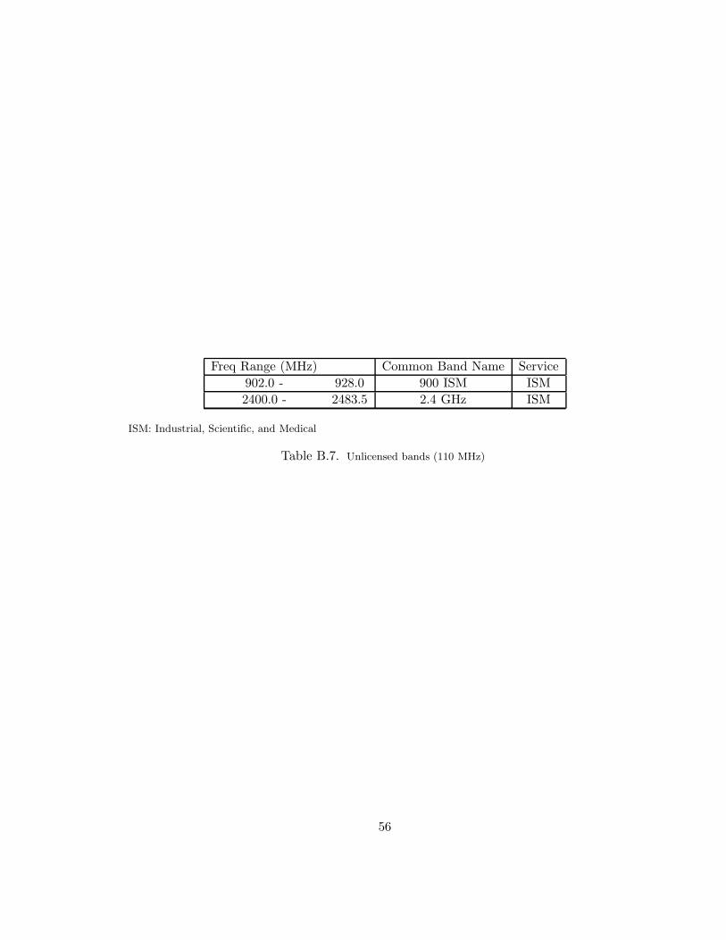
Freq Range (MHz) Common Band Name Service
902.0 - 928.0 900 ISM ISM
2400.0 - 2483.5 2.4 GHz ISM
ISM: Industrial, Scientific, and Medical
Table B.7. Unlicensed bands (110 MHz)
56

![Investigative Analysis of Cognitive Radio Wireless Model ...2.1 Cognitive Radio Cognitive radio was inspired by [10] as evolving technology from software defined radio to offer solution](https://img.pdfslide.us/doc/110x75/5f050a4e7e708231d410f601/investigative-analysis-of-cognitive-radio-wireless-model-21-cognitive-radio.jpg)