On the Factors that A ect Airline Flight Frequency and ... · PDF fileOn the Factors that A ect Airline Flight Frequency and Aircraft Size Vivek Pai ... force or the proportion of

On the Factors that Affect Airline Flight Frequency andAircraft Size∗

Vivek PaiUniversity of California, Irvine

Department of Economicse-mail: [email protected]

November 5, 2007

Abstract

This paper assesses the determinants of aircraft size and frequency of flights on airline routesby considering market demographics, airport characteristics, airline characteristics and routecharacteristics. The paper shows that frequency and aircraft size increase with population,income, and runway length. An increase in the proportion of managerial workers in the laborforce or the proportion of population below the age of 25 results in greater frequency withthe use of small planes. Slot constrained airports and an increase in the number of nearbyairports lead to lower flight frequency with the use of smaller planes. Hubs and low costcarriers are associated with larger plane sizes and higher frequency, while regional airlineownership leads to higher frequency and the use of smaller planes. An increase in distancebetween the endpoints leads to lower frequency with the use of larger planes. As airport delayrises, airlines reduce frequency and use smaller planes, though when airport cancellations rise,flight frequency increases with the use of larger planes. This finding suggests airlines utilizefrequency and aircraft size to hedge against flight cancellations.

∗I thank Jan Brueckner, Volodymyr Bilotkach, Linda Cohen, Iris Franz, Nick Rupp, Ken Small, Kurt Van Dender,and Kat Wong for their feedback. I’m grateful to the University of California Transportation Center for generousfinancial support. Credit for any errors remains with the author.

1

1 Introduction

Flight delays have become rampant in the airline industry. US on-time performance for the

summer of 2007 has been the worst on record, with over 30 percent of all commercial flights

delayed. Airlines blame bad weather and an outdated air traffic control system. Government

officials blame airlines for scheduling more flights than the system is designed to handle. At

the same time, airlines are utilizing small regional aircraft, which are capable of carrying

between 30 and 100 passengers, in greater numbers than ever before. These smaller planes

utilize the same resources as larger planes in terms of landing slots and air traffic control, while

carrying fewer passengers than mainline aircraft. What factors lead airlines to exacerbate the

problems of over-utilized infrastructure by using smaller aircraft with greater frequency over

larger aircraft? This paper attempts to answer this question by examining the determinants

of aircraft sizes and the frequency of flights between airports.

Airlines may choose to serve a market1 with a particular aircraft size and frequency due to

various population, market, and airport characteristics. A market that has a high concentration

of passengers with high time costs (business travelers) might be served by smaller aircraft with

greater frequency, while a market with a high concentration of low time cost passengers (leisure

travelers) might be serviced by larger aircraft with lower frequency. Conversely, markets with

a high concentration of business or affluent passengers could benefit from the use of larger jets,

as they have more first class seats, than markets with fewer business or affluent passengers.

Distance is also a significant factor in the use of a particular aircraft type on a route. As

the distance between the two endpoints increases, longer-range (and thus larger) aircraft are

needed.1In this paper, the term market is used to describe a direct route between two cities. In actuality a city-pair

market is the market for travel between two cities without regard to the route taken. For example, the routing mayinvolve a connection at a hub airport rather than a non-stop flight. The paper’s convenient, but inexact, use of theterm market should be borne in mind.

2

The determinants of aircraft size and frequency have major policy implications, especially

with respect to congestion and landing fees. Federal Aviation Administration officials have

proposed aircraft size targets at New York’s LaGuardia airport, as airlines’ use of regional jets

over mainline jets in the airport’s limited number of landing slots has led to high congestion

and under-utilization of passenger terminals. A minimum size requirement, however, may lead

to under-provision of desired flight frequencies or over-provision of seat capacity. Thus, while

a seat requirement may lead to more efficient use of terminal infrastructure, such a policy may

ultimately reduce total welfare. A thorough understanding of the determinants of aircraft size

and flight frequency will allow policy makers to better judge the outcomes of proposed policies.

Researchers have paid some attention to the determinants of aircraft size and frequency in

city-pair markets. Bhadra (2005) constructs a multinomial logit regression using the number

of passengers, distance, and the type of airport hub at the route endpoints to explain air-

craft choice in the US. A self-noted shortcoming of the model is that neither airline behavior,

nor economic factors affecting passenger demand, are considered in explaining aircraft choice.

Givoni and Rietveld (2006) take a different approach by considering the implications of route

factors and airport characteristics on the aircraft size decision. Using OLS, the authors inves-

tigate the impact of distance, market size, market concentration, slot constraints, hub status,

and the number of runways on aircraft choice on over 500 routes in the US, Europe and Asia.

Givoni and Rietveld find that the choice of aircraft size is mainly influenced by route charac-

teristics, including distance, level of demand, and competition. The authors further find that

airport characteristics, such as the number of runways and whether the airport is a hub or slot

constrained, do not influence aircraft choice.

Other factors may also influence aircraft sizes. An airline may opt to use larger aircraft on

a route due to economies of scale in aircraft operation.2 This effect, however, may be offset

2As noted by Babikian, et al (2002), smaller regional jets have lower fixed costs, though their operating costs are

3

by higher labor costs. Pilots receive higher salaries for flying larger aircraft, leading airlines

to prefer in some cases the use of smaller aircraft in short-haul, high density markets (Wei

and Hansen, 2003). Forbes and Lederman (2005) consider the relationship between service

quality and the integration of regional carriers with major airlines. On routes where schedule

disruptions are costly to the major carrier and likely to occur (i.e., on hub routes and routes-

prone to bad weather), the authors show that major airlines are likely to rely on their regional

carrier subsidiaries, rather than on independent regional carriers. Thus, factors such as unit

costs and relationship to regional carriers may play a factor in an airline’s aircraft size and

frequency decisions.

This study focuses on the US market and uses 4 groups of explanatory variables to in-

vestigate the determinants of aircraft size and flight frequency: market demographics, airport

characteristics, airline characteristics and route characteristics. These explanatory variables

provide insight into the demand characteristics and operational constraints that airlines face

in making aircraft size and frequency decisions. This approach differs from past studies that

consider operational constraints without any attention to demand factors. In a departure from

the current literature, the study uses several continuous variables as hub controls instead of

a dummy variable. Such an approach allows for deeper analysis of “focus cities,” cities that

have service to many destinations, but are not considered a hub by the carrier. In addition,

the impact of delays and cancellations on frequency and aircraft size are considered.

This study finds that frequency and aircraft size increase with population and income

at the route endpoints. An increase in the proportion of managers in the workforce or the

percentage of the population below 25 years of age results in greater frequency and the use of

smaller planes. With respect to airport characteristics, as consistent with previous literature,

an increase in runway length results in higher frequency and larger plane sizes. Airport slot

higher. Conversely, large jets have low operating and high fixed costs.

4

constraints and the existence of more airports in the vicinity lead to lower flight frequency

and smaller planes. Hub airports and low cost carriers are associated with larger plane sizes

and higher frequency, though regional airline ownership by the major carrier leads to higher

frequency and the use of smaller planes. An increase in distance between the endpoints leads

to lower frequency and the use of larger planes. An increase in average delay at an endpoint

leads airlines to provide lower frequency and to use smaller planes, though an increase in

cancellations leads to higher flight frequency and use of larger planes. This finding suggests

that airlines utilize aircraft size and frequency to hedge against flight cancellations.

The paper has 5 sections. The following section introduces a theoretical framework to

motivate the empirical work. Section 3 provides a description of the data, while Section 4

discusses empirical results. The last section offers some concluding remarks.

2 Theoretical Framework and Implications

To understand the implications of demographics on aircraft size and frequency, a review of

the monopoly scheduling model of Brueckner (2004) is useful. For simplicity, the airline serves

three equidistant cities, A, B, and H, as shown in Figure 1. Demand for travel exists between

each pair of cities, yielding three city-pair markets: AH, BH, and AB. In a point-to-point

network, the airline operates flights between each pair of cities, so that nonstop travel occurs

in each city-pair market. In a hub-spoke network, the airline only operates flights to the hub

H. Therefore, flights in the hub-spoke network carry both local (passengers in markets AH or

BH) as well as connecting passengers (passengers in market AB).

Travel demand is identical in the three city-pair markets, and thus the airline faces the same

inverse demand function in each market, derived as follows. Passengers must commit to travel

before knowing their preferred departure time. Letting T denote the time circumference of the

5

circle (representing a day), the passenger’s utility is dependent on expected schedule delay,3

which equals T/4f , where f is the number of (evenly spaced) flights operated by the airline.

Letting ν denote a disutility parameter, the cost of schedule delay is νT/4f . Setting γ equal

to νT/4, this cost becomes γ/f . In addition, connecting passengers have to incur additional

travel costs (including extra travel time as well as the inconvenience of changing planes) that

local passengers avoid. The extra cost of traveling indirectly is denoted µ. Following Brueckner

(2004), the airline’s inverse market demand function is then

p = α− βq − γ/f − µ, (1)

where p is the price and q is the number of passengers.

Letting s denote the number of seats per flight, the cost function of the airline involves two

parameters, a fixed cost, θ, and a marginal cost per seat, τ :

c(s) = θ + τs. (2)

For simplicity, all seats on an aircraft are assumed to be filled, which implies that the number

of seats per flight must equal total passengers divided by the frequency of flights:

s = q/f. (3)

With the above demand and cost functions, profit functions for both the point-to-point and

hub-spoke networks can be derived. In a point-to-point network, the total cost for each route

is equal to fc(s). After substituting (3) into (2) and rearranging, total costs per route can be

3To derive expected schedule delay, suppose that the airline’s flights are evenly spaced around the clock, withT denoting the number of available hours. Then, letting f denote the number of flights, the time interval betweenflights is T/f. The average time between flights is T/2f , and expected schedule delay is T/4f, assuming a uniformdistribution of desired departure times.

6

written as fθ+τq. Subtracting the total cost per route from revenue per route, as obtained by

multiplying (1) by the number of passengers on the route, profit for a point-to-point network

equals

πpp = 3[(α− βq − γ/f)q − fθ − τq], (4)

where the factor of 3 reflects the 3 routes in the network, as presented in Figure 1. Note that

in the point-to-point network, µ is 0, as all passengers travel direct to their destination and

therefore do not incur any additional travel time costs.

The profit function for a hub-spoke network differs from that in a point-to-point network.

In the hub-spoke case, flight frequency on each of the two routes is denoted fh. Local passengers

are denoted qh, while connecting traffic is denoted Q. Since a hub-spoke network creates an

asymmetry between the AB market and the other two direct markets, qh and Q will not be

equal. Likewise, the fare for connecting passengers in the AB market is set independently of

the fares for local passengers, not being simply the sum of the fares from A to H and from H to

B. From (1), local fares are given by ph = α− βqh − γ/fh. Like in the point-to-point network,

local passengers travel direct and therefore do not incur any additional travel time costs, so

that µ = 0. However, since AB passengers incur a connection cost, the fare in the AB market

is equal to P = α− βQ− γ/fh − µ.

Since connecting passengers must travel on both hub-spoke routes, passenger volume on

each route is equal to is equal to qh +Q, resulting in an aircraft size of sh = (qh +Q)/fh. After

substituting the aircraft size on hub-spoke routes into (3) and multiplying by the number of

routes flown, total hub-spoke network costs are 2[fhθ + τ(qh + Q)]. With the airline earning

revenue from two local markets as well as the connecting market, hub-spoke network profit is

πhs = 2qh(α− βqh − γ/fh) +Q(α− µ− βqh − γ/fh) − 2θfh − 2τ(qh +Q). (5)

7

After analysis of the first order conditions for profit maximization, Brueckner (2004) finds the

following results:

1. Flight frequency increases, irrespective of network type, when:

(a) the demand intercept α rises or the demand curve slope β falls (shifting the demand

curve outward).

(b) fixed cost θ or marginal seat cost τ falls.

(c) schedule delay cost γ rises.

2. As the cost of layover time for connecting passengers, µ, increases, hub-spoke frequency

fh, local hub-spoke passengers qh and connecting hub-spoke passengers Q all decline.

3. Irrespective of network type, aircraft size s increases when:

(a) the demand intercept α rises or the demand curve slope β falls.

(b) marginal seat cost τ falls.

4. Flight frequency is higher in a hub-spoke network than in a point-to-point network

5. Aircraft sizes are larger in a hub-spoke network than in a point-to-point network

With the comparative-static results presented above, expected empirical outcomes can

be predicted. Since demand for travel is cyclical, with higher demand during the summer,

quarterly dummy variables should indicate higher frequency and larger plane sizes during peak

travel periods, which are the 2nd and 3rd quarters. Population would also shift the demand

intercept α in the theoretical model. Thus, as population levels (α) increase, frequency and

aircraft size should increase. Since households with high incomes also demand more air travel,

an increase in income should also raise frequency and aircraft size.

Business travel is undertaken by managers who have high values of time. Therefore, man-

agers would have a high γ, which results in high flight frequency in markets that serve managers.

High income households also have a high opportunity cost of time and thus, like managers,

have a high γ, leading to higher frequency in high-income markets. This effect reinforces the

8

increase in flight frequency brought about through the higher demand associated with high

incomes. But due to their high values of time, managers and high income households also have

a high cost of layover time µ. With a high γ value raising frequency and a high µ lowering it,

the ultimate effect on frequency of an increase in the number of managers and high income

households is thus ambiguous. This ambiguity disappears, however, in a point-to-point net-

work, where µ = 0. Also note that the effect of an increase γ on aircraft size is ambiguous.

Though these results are derived for a monopoly model, similar results hold in a competitive

model (Brueckner and Flores-Fillol, 2007).

Low cost carriers (LCCs), like Southwest, operate point-to-point networks. Therefore, a

LCC control variable might be expected to have a negative effect on aircraft size and frequency,

given predictions (4) and (5) above. These predictions, however, may not hold given the

contrasting markets served by LCCs and traditional, hub-spoke carriers. Hub-spoke carriers

often serve small towns through the use of turboprop and regional jets, while low-cost carriers

usually serve larger cities with larger aircraft. This disparity can be seen in Table 1, where

cities that have service by a LCC are much larger than cities that do not have such service.

Since this service pattern means that LCCs do not own turboprops and regional jets, LCC

service might then be associated with larger than average aircraft. In addition, while the model

implies higher frequency in hub-spoke networks, suggesting that the LCC effect on frequency

should be negative, this effect may not be present given the different nature of LCCs.

Past empirical studies have shown the effect of hub endpoints to be positive for both

frequency and aircraft size (Givoni and Rietveld, 2006), as theoretically stated above. This

paper, unlike related studies, uses the share of passengers connecting at the airport and number

of destinations served as hub controls instead of a dummy variable. Hub cities have high

9

connecting shares along with service to a large number of endpoints. Some non-hub cities,

however, have appreciable values of these variables, as seen in Table 8 in the appendix. In

line with past literature, it is expected that aircraft size and frequency rise as the share of

passengers that connect and the number of destinations increase. In addition, as suggested

by Forbes and Lederman (2005), major airlines that own regional carriers may have a greater

ability to dictate flight schedules and aircraft usage than carriers that rely on contract partners.

This effect would suggest that major ownership of a regional carrier would allow greater flight

frequency and the use of smaller planes.

Past literature has shown that, as distance between the two endpoints increases, aircraft

size increases and frequency decreases (Givoni and Rietveld, 2006). In addition, for large

aircraft to land and take off, an airport must have longer runways. Therefore aircraft size

should have a positive relationship with runway length.

For a fixed population, the presence of nearby airports will split passengers among several

airports and therefore result in lower frequency and the use of smaller aircraft at a given

airport. Givoni and Rietveld (2006) also find that slot constraints lead to smaller aircraft,

though the result is not statistically significant. While Givoni and Rietveld (2006) do not

consider frequency, it would be expected that slot constraints would lower flight frequency.

Finally, delays and cancellations cause uncertainty for passengers and airlines in terms of

expected arrival times and operations, respectively. While Rupp and Homes (2005) suggest

that airlines will not cancel flights if frequency is low, the effect of operational uncertainty, as

measured by airport-level delays and cancellations, on aircraft size and frequency is hard to

predict.

10

3 Empirical Model and Data

To conduct this study, the following regression model is estimated:

Gijkt = αijkt + β1Wi + β2Wj + β3Xikt + β4Xjkt + β5Yk + β6Zij + vijkt (6)

where Gijkt is the dependent variable (frequency or aircraft size) on the route from airport i

to airport j on airline k in month t, and vijkt is the error term. Many studies that focus on

the airline industry remove directionality in the data (i.e., treat flights from j to i the same

as flights from i to j). Due to the nature of the hub control variables used in this study,

however, the directional nature of the data is retained. Wi and Wj are vectors of airport

specific characteristics as well as population demographics for the cities where airport i and

j are located, respectively. Xikt and Xjkt are vectors of airline-specific hub and operational

characteristics for each airport in a given month. Yk and Zij are vectors of airline and route

specific characteristics, respectively.

Data for the dependent variables, scheduled departures per month and seats per departure,

are constructed from the Department of Transportation’s (DOT) 2005 T-100 service-segment

database. Information contained in the T100 is derived from Form 41, which large scheduled

carriers4 have been required to submit since 1990. Among other information, the form contains

numbers of departures and seats by carrier for each non-stop US route segment on a specific

plane type in a given month.

Beginning in the third quarter of 2002, the DOT required all air carriers, including small

4The BTS defines large certificated air carriers as airlines that hold Certificates of Public Conve-nience and Necessity issued by the U.S. Department of Transportation (DOT) and operate aircraft withseating capacity of more than 60 seats or a maximum payload capacity of more than 18,000 pounds.(http://www.bts.gov/publications/airport activity statistics of certificated air carriers/)

11

and regional air carriers, to submit data. To assign regional carriers to major airlines, annual

10K reports filed each year with the Securities and Exchange Commission for all the major and

regional airlines are analyzed to identify partnerships. Assignments are subsequently checked

for accuracy by cross-checking regional carrier route maps and the schedules of their major

carrier partners to ensure that the routes are properly assigned. The resulting assignments

can be found in Table 2.

To insure that flights are in fact regularly scheduled, the data is limited to observations

where the carrier has more than 20 scheduled departures per month on a specific plane type.

All flights in a month by a major airline on a route are then collapsed into a single observation.

Thus, an observation in the analysis come from summing flights on a route operated by a major

airline and its partners over all plane types in a given month. Summary statistics for the data

can be found in Table 3

Data for the explanatory variables come mostly from a variety of government databases,

including the 2000 US Census, the DOT’s Origin and Destination Survey and On-Time Per-

formance datasets, and the Federal Aviation Administration’s National Flight Data Center’s

Airport Runways Data Table. A brief description of the databases and variable construction

follows.

The vector of market demographic data includes the proportion of households with an

annual income greater $75,000, the percentage of managerial workers (obtained by summing

all workers in managerial occupations), and the proportion of population under 25 years of

age, as well as total population. As airports serve an area larger than their name implies,

airports are matched to a Metropolitan Statistical Area5 (MSA), with data for each endpoint

5A Metropolitan Statistical Area is defined as a core area containing a large population nucleus, together withadjacent communities having a high degree of economic and social integration with that core.

12

used in the regression, as noted in equation (6). Data come from the 2000 Census, gathered

from the 2007 State and Metropolitan databook. The use of MSA data, however, limits the

data to city pairs within the contiguous 48 United States. More details on the census data

and attribution to an airport can be found in the appendix.

Endpoint airport characteristics data, which include the number of nearby airports, maxi-

mum runway length and slot constraints, come from several datasets. Maximum runway length

and latitude and longitude are obtained from the Federal Aviation Administration’s National

Flight Data Center’s Airport Runways Data Table. To identify nearby airports, the longitude

and latitude is used to calculate the distance between all airports in the US via the great circle

formula. The number of airports in the vicinity is then the count of all airports that are within

75 miles of the given endpoint. Slot Constrained is a dummy variable that takes on the value 1

if the origin or destination is New York’s JFK or LaGuardia, Chicago O’Hare, or Washington

National.

In this study, two variables are used as a proxy for hub airport status: number of destina-

tions served and the proportion of passengers that are connecting to other flights at the airport,

each measured at the airline level. The number of destinations served from the endpoint is

the sum of destinations served by the carrier derived from the T100. Connecting shares are

computed by analyzing the DOT’s 2004 DB1B dataset. The DB1B contains, among other

things, information on a passenger’s origin, destination and routing. To derive connecting

shares, individual coupons are analyzed to determine the actual route. Passengers that pass

through an airport without a break in their itinerary are determined to be connecting. Both

hub proxy variables are computed for the year 2004 to avoid endogeneity.

Airline identity is preserved in the dataset, though individual airline fixed effects are not

13

included in the model. When the model was estimated with airline fixed effects, all of the

population characteristic variables were rendered insignificant. Airline identities are, however,

used to construct several control variables. An LCC dummy takes on the value 1 when the

airline is Southwest, Airtran, JetBlue, or ATA. A dummy variable indicating ownership of

regional carriers takes on the value 1 when the major owns a regional carrier. In 2005, this

criterion was satisfied for American and Delta Airlines. Their owned regional carriers can be

found in Table 2.

Route characteristics include distance between the two endpoints and a leisure variable.

The distance between the two endpoints, as used in this study, is reported in the T100 database.

Leisure takes on the value 1 when either endpoint is Las Vegas (LAS) or Orlando (MCO).

Finally, the effects of delay and cancellations are considered. Delayed and cancelled flight

information is derived from the DOT’s on-time database. This database contains, among

other items, delay and cancellation data on every flight operated by the major U.S. carriers.

To avoid endogeneity, data from the year 2004 are used. Delay is calculated as the sum of the

absolute value of arrival and departure delay at the origin and destination, respectively, for the

given airline. In this fashion, arriving early is equivalent to arriving late.6 Whereas arrival and

departure delays are attributable to the origin and destination, the data reports a particular

flight as cancelled, without attribution to the source. Cancellations are, therefore, attributed

to both the origin and destination. Cancellations, as used in the analysis, are calculated as

the percentage of flights the airline cancels at each airport.

Despite the fact that delay and cancellations are lagged and measured at the airport level,

6This approach can be justified as follows. Suppose a passenger is to picked up at the airport at a predeterminedtime. If their flight arrives early, the passenger must wait for their greeter, whereas if the flight arrives late, thegreeter must wait for the passenger. In essence, either party would be confronted with a waiting cost, and thisconstruction accounts for this cost.

14

they may still be endogenous to aircraft size and flight frequency on individual routes. Thus,

precipitation at the endpoints and aircraft movements per runway are used as instrumental

variables in a two-stage least squares regression that treat delays and cancellations as endoge-

neous. Historic precipitation data is gathered from the U.S. National Oceanic & Atmospheric

Administration (NOAA) website. The number of aircraft movements per runway is derived

by dividing the number of takeoffs and landings by the number of runways, as reported in the

FAA’s Airport Runways Data Table.

4 Empirical Results

The results of the regressions with frequency and aircraft size as the dependent variables are

presented in Tables 4 and Table 5, respectively. The first column in each table is the base

specification. Base-specification results for flight frequency and subsequently aircraft size are

now presented, before turning attention to the effect of delay and cancellations.

4.1 Flight Frequency

Time of year and population characteristics play a significant role in determining flight fre-

quency. As expected, the second and third quarters, which correspond to the spring and peak

summer travel periods, have the highest frequency. The 4th quarter, which is omitted, has the

lowest frequency, and the 1st quarter coefficient is statistically insignificant. As population

increases, frequency increases, as suggested by the theoretical framework and confirmed by

the positive population coefficients. Specifically, an increase of 100,000 people at the origin

or destination results in an increase of .73 or .76 flights per month, respectively. Increased

household income also causes an increase in frequency, with each percent-point increase in

15

households earning more than $75,000 resulting in 2.7 additional flights per month.

Of all population characteristics, the proportion of managers in the workforce has the

largest effect. An additional percentage-point of managers in the workforce at the origin or

destination results in nearly an additional flight per day, or approximately 20 or 24 flights per

month, respectively. The higher frequencies for routes with high incomes and many managers

suggest that airlines are attentive to schedule delay, as suggested by the theoretical framework.

Finally, an increase in the proportion of the population below 25 years of age leads to a slight

increase in flight frequency. This effect may indicate that families with young children and

college students travel more than older people.

The presence of vicinity airports, among other airport characteristics, has a major impact

on flight frequency. As can be seen, each additional airport within a 75 mile radius results

in approximately 9 fewer flights per month. The presence of additional airports would split

the metropolitan area’s traffic, resulting in lower frequency at each airport. In addition, more

airports in an area may lead to additional airspace congestion, and therefore result in lower

flight frequency. For example, in the New York City area, with 3 major airports and several

smaller ones, airspace coordination is a major problem. Runway length also positively affects

flight frequency, though its effect may be more indirect. Airports with long runways also tend

to have more runways, and are thus capable of having more aircraft movements.

Hubs are associated with greater frequency. One additional destination results in an ad-

ditional .6 flights per month. A one percent increase in the share of connecting passengers

leads to an increase of 27 and 16 flights per month at the origin and destination, respectively.

Finally, low cost carriers have greater frequency than non-low cost carriers.

Distance plays a major role in determining flight frequency. Every 1000 mile increase in

16

distance results in 62 fewer flights over the course of a month, or 2 fewer flights per day. There

are two explanations for this trend. As the distance between the two endpoints increases,

planes can make fewer trips over the course of a day. In addition, as distance increases, the

chance that a hub city is on the flight path increases. Unless a compelling factor exists,7 an

airline might opt to route the flight through the hub. Leisure routes have greater frequency,

with an increase of more than 1 flight per day if the route involves Las Vegas or Orlando.

The second specification in Table 4 adds slot constraints and major ownership of regional

carriers. As can be seen, the presence of a slot-constrained airport on the route results in

a drop of nearly one flight day compared to routes without such airports. This finding is

consistent with the rationale for slot constraints, namely, that there should be fewer flights.

Major ownership of a regional carrier results in nearly an additional flight per day. Forbes

and Lederman (2005) suggest regional ownership allows major carriers to mitigate problems

that arise when unforeseen schedule disruptions occur. Thus, the ability to mitigate problems,

should they arise, allows airlines greater flexibility, and as shown, results in greater frequency.

4.2 Aircraft Size

Attention now turns to aircraft size, as measured by seats per departure. Time of year and

population characteristics play a significant role in determining aircraft size. As compared to

the omitted 4th quarter, all quarters have larger aircraft sizes, with the 1st and 2nd quarter

having the largest sizes. Consistent with the theoretical model, aircraft size increases as

population increases. An increase of 100,000 people at the origin or destination results in an

additional .09 or .07 seats per departure, respectively. The small size of this effect suggests that

7Brueckner and Pai (2007) explore the determinants of point-to-point service.

17

higher travel demands are met mainly through greater frequency. An increase in household

income in an area also results in larger aircraft size: 1 or .8 more seats for every percent

increase in households earning more than $75,000 at the origin or destination, respectively.

An increased share of managerial workers, however, results in a decrease of approximately

1.5 seats per departure. Coupled with the fact that airlines increase frequency as the share

of managerial workers increases, this finding indicates that airlines use smaller airplanes and

have higher frequency on routes between endpoints with a large share of managers. A higher

youth proportion also results in a decrease in plane size.

Airport characteristics play a large role in determining aircraft size. Runway length is often

a constraint on aircraft size. Larger planes require longer runways to take off and land, and

this connection is confirmed by the positive relationship between size and runway length. An

additional 1000 feet of runway results in an increase of 1.54 or 1.38 seats per departure at

the origin or destination, respectively. The presence of nearby airports leads to a decrease in

aircraft size. As with frequency, this effect is expected, as multiple airports would split the

passenger pool over all airports in the area. In order to keep planes full, airlines would utilize

smaller aircraft with lower frequency at each airport in a multiple-airport metro area.

Airlines utilize larger planes on routes that involve hubs. As can been seen from the

coefficients on the hub variables, a one percentage point increase in connecting share results

in nearly a 7 seat per departure increase in aircraft size. In contrast, service to an additional

destination increases aircraft size by less than one quarter of a seat. As expected, low cost

carriers have more seats per departure. In addition to serving larger areas, low cost carriers

often have a single aircraft type, usually in the 120-140 passenger range. This contrasts with

network carriers, which utilize multiple plane types that range from 30-300+ seats.

18

Finally, distance is a major factor in plane size decisions, as shown by both Bhadra (2005)

and Givoni and Rietveld (2006). As the distance between the two endpoints increases, longer-

range (and thus larger) aircraft are needed. This effect is confirmed by the positive relationship

between distance and seats per departure. A 1000 mile increase in distance between the

endpoints results in an increase of nearly 30 seats per departure. Leisure routes also have

larger aircraft, with an increase of more than 15 seats if the route involves Las Vegas or

Orlando.

The second specification in Table 5 adds slot constraints and major ownership of regional

carriers to the model. As can be seen, the presence of a slot constrained airport on the

route results in a small drop in seats per departure, though this coefficient is statistically

insignificant. Dresner et al. (2002b) find that slot controls, gate constraints (due to exclusive

leasing arrangements between airlines and airports), and gate utilization during peak periods

all contribute to airline yields. Thus, airlines have an incentive to prevent their excess slot and

gate capacity from being used by their competitors. By utilizing smaller aircraft, airlines are

able to hold their slots and gates, while limiting capacity (and as a consequence, not having

to reduce prices due to competition.)

Major ownership of regional carriers results in a 1.74 decrease in seats per departure.

This finding suggests that majors that own regional carriers have greater flexibility in utilizing

smaller aircraft. Pilot unions often limit the use of various plane sizes through “scope clauses,”

which limit the use of of small aircraft. Presumably, carriers that own regional subsidiaries

have greater flexibility in deploying aircraft of various sizes on routes than carriers that do not

own regional subsidiaries.

19

4.3 Summary

The preceding results are summarized as follows. Frequency and aircraft size increase with

population and income. An increase in the proportion of managers in the workforce and in the

share of population below 25 years of age results in greater frequency and the use of smaller

planes. An increase in runway length results in higher frequency and larger plane sizes. Routes

on which airports are slot constrained and have more competing airports nearby have lower

flight frequency and smaller planes. Hubs and low cost carriers are associated with larger plane

sizes and higher frequency, and regional-airline ownership leads to higher frequency and the

use of smaller planes. An increase in distance between the endpoints leads to lower frequency

and the use of larger planes. The implications of delay and cancellations on aircraft choice

and flight frequency are discussed in the next section.

4.4 Impact of Delay and Cancellations

Delay and cancellations on a route often result in disruptions throughout the airline’s network.

Thus, in order to minimize schedule disruptions, airlines may have an incentive to provide lower

frequency on routes that are delay and cancellation-prone. This section analyzes the effect of

delays on flight frequency and subsequently aircraft size, before turning attention to the effect

of cancellations on frequency and aircraft size.

Delays impact flight frequency. As can be seen in Table 6, column (a), a one minute

increase in delay at the origin or destination airport results in a .28 or .15 decrease in the

number of flights per month, respectively. Given the possible simultaneity between delay and

the dependent variable, a two-stage least squares model was also estimated using precipitation

and aircraft movements per runway as instruments for delay. As shown in Table 6, column (b),

20

qualitative results are the same under the 2SLS specification, although the magnitude of the

delay effect rises to a 2 flight per month decrease in frequency. Thus, it appears that airlines

are trying to limit disruptions to their schedule by reducing frequency at delay-prone airports.

Like frequency, aircraft size is impacted by delay. As can been seen in Table 6, column

(c), a one minute increase in average delay results in nearly a one-quarter seat per departure

decrease in plane size. One plausible explanation is that short-haul routes are more likely to

be delayed, and that short routes are, in-turn, serviced by small planes. As in the frequency

case, a 2SLS regression was estimated using precipitation and aircraft movements per runway

as instruments for delay at the airport level. The qualitative results of the 2SLS specification

are similar to the OLS results, though the magnitude of the delay effect decreases to 1.6 or .47

seats per departure at the origin or destination, respectively.

Cancellations play a significant role in the flight frequency decision. As can been seen

in Table 7, column (a), an increase in the share of cancelled flights at the route endpoints

results in greater frequency. While this finding appears counterintuitive from an operations

standpoint, it makes sense. Recall that the cancellation data is lagged relative to the frequency

variable. Thus, in response to past cancellations, airlines are scheduling more flights, and the

reason appears to be that greater flight frequency allows airlines to cancel a flight without

causing passengers significant inconvenience. In addition, as suggested by Rupp (2005), airlines

may choose to not cancel infrequent flights in order to maintain their schedules following the

cancellation. Additional frequency allows an airline to cancel flights without major schedule

disruptions.

Cancellations also influence aircraft size. As shown in Table 7, column (c), cancellations

lead to larger aircraft size. The apparent explanation is that, if an airline is likely to cancel

21

a flight, additional capacity on the remaining flights is necessary to service all its passengers.

These findings suggest that airlines use both frequency and aircraft size to hedge against

cancellations.

Using precipitation and aircraft movements per runway as instruments for cancellation, the

2SLS results are similar to the OLS results: airlines provide higher frequency and use larger

planes on routes with cancellation-prone endpoints. Note the statistical insignificance of the

coefficients on many of the population characteristics and the share of connecting passengers

in Table 7, column (d). This outcome suggests that the instruments capture some of the

heterogeneity previously captured by managerial share of the workforce and the connecting

share.

5 Conclusion

The US airline industry has experienced rampant delays, and expectations are that the delay

problem will become more severe. Airlines are utilizing smaller planes with greater frequency,

while the government is relying on an air traffic control system that was not meant for handling

the number of flights being flown. This paper explores the factors that might lead airlines

to exacerbate the problems of over-utilized infrastructure by examining the determinants of

aircraft sizes and the frequency of flights between airports.

The paper shows that frequency and aircraft size increase with population and income.

An increase in the share of managerial workers or the proportion of the population below 25

years of age results in greater frequency and the use of smaller planes. An increase in runway

length results in higher frequency and larger plane sizes. Slot constrained airports and an

increase in nearby airports lead to lower flight frequency and smaller planes. Hub airports and

22

low cost carriers are associated with larger plane sizes and higher frequency, though major

airline ownership of regional carriers leads to higher frequency and the use of smaller planes.

An increase in distance between the endpoints leads to lower frequency and the use of larger

planes. An increase in delay at the route endpoints leads to lower frequency and smaller planes.

An increase in cancellations, however, leads to higher frequency and the use of larger planes.

These findings suggest that airlines utilize frequency and aircraft size to hedge against flight

cancellations, and it warrants further exploration.

Various proposals have been suggested to ease delays at US airports. In the past, gov-

ernment officials have asked airlines to voluntarily reduce frequency during peak periods to

cut congestion. By exposing the determinants of flight frequency, however, the results in this

paper show the pitfalls in this kind of bureaucratic approach. In particular, the paper’s find-

ings show that high frequencies represent the airlines’ response to the demand for convenient

service by time sensitive passengers, who have high incomes or managerial jobs. Arbitrary

frequency restrictions prevent the fulfillment of these demands in a efficient manner. A better

approach would be to adopt congestion pricing, which would allow time sensitive passengers

to be served at times of their choosing if they are willing to pay higher fares, which would

embody the congestion charges for peak-hour travel.

23

Figure 1: Network Configuration

Table 1: Average Demographic Characteristics for Cities with and without LCC Service

Without LCC service With LCC servicePopulation 291,124 2,365,669Household income over 75k 16.86% 23.78%Percent Managers 33.78% 46.70%Percent Young 36.51% 35.11%

24

Table 2: Regional Carrier Assignment

Major Carrier Regional CarrierAmerican (AA) American Eagle∗

Executive Airlines∗

Regions AirChautauqua AirlinesTrans States

Alaska (AS) Horizon∗

Continental (CO) ExpressJetCommutairColganSkywest

Delta (DL) ASA/Atlantic Southeast Airlines∗

Comair∗

SkywestChautauqua Airlinesa

RepublicFreedomb

Northwest (NW) Mesaba AirlinesExpress Airlines

United (UA) Air Wiconsinc

GoJetShuttle AmericaTrans StatesSkywestd

MesaChautauqua AirlinesColgane

US Airwaysf Air WisconsinChautauqua AirlinesMesa

Airlines that serve multiple airlines are assigned based on hub identities, as noted in bold in Table8. Asterisks indicate major owned regional.

aOnly routes involving cities in Florida and Raleigh-Durham (RDU)bOnly routes involving Orlando, FL (MCO)cOnly on routes involving Chicago O’hare (ORD) and Washington Dulles (IAD)dIncluding routes involving Portland, OR (PDX), Medford, OR (MFR), and Eureka-Arcata, CA (ACV)eOnly routes involving Washington Dulles (IAD)fThe following airlines, which are observed in the T100 database, are also assigned to US Airways: PSA Airlines,

Piedmont, and America West

25

Table 3: Summary Statistics

Variables Means

Time Control Variables1st Quarter .2422nd Quarter .2503rd Quarter .256

Population Characteristics

Origin Population (in hundred thousands) 38.637Destination Population (in hundred thousands) 39.426Origin Income above $75,000 26.273Destination Income above $75,000 26.529Origin Percent Managers 0.427Destination Percent Managers 0.425Origin Percent Young 35.107Destination Percent Young 35.095

Airport Characteristics

Origin Maximum Runway Length 10.912Destination Maximum Runway Length 11.027Vicinity Airports near Origin 2.259Vicinity Airports near Destination 2.272Delay at Origin (in minutes) 29.570Delay at Destination (in minutes) 29.583Operations per runway at Origin 7031.54Operations per runway at Destination 7288.53Precipitation at Origin (in inches) 2.983Precipitation at Destination (in inches) 2.981

Airline CharacteristicsNumber of Destinations from Origin 44.216Number of Destinations from Destination 21.234Share of Connecting Passengers at Origin 0.181Share of Connecting Passengers at Destination 0.190Low Cost Carrier 0.229Major Carrier owns Regional Carrier 0.327

Route CharacteristicsDistance (in thousands of feet) 0.809Leisure Route 0.074Aircraft Size 113.475Frequency 127.590Average Delay 6.737Cancelled Flights 0.025

26

Table 4: Frequency

Dependent Variable Departures Scheduled

Intercept −164.7∗(8.564)

−155.3∗(8.45)

Time Control Variables1st Quarter 1.315

(1.016)1.365(1.001)

2nd Quarter 5.489∗(1.005)

5.603∗(0.991)

3rd Quarter 6.140∗(0.998)

6.001∗(0.986)


Origin Population 0.732∗(0.016)

0.771∗(0.016)

Destination Population 0.763∗(0.083)

0.793∗(0.016)

Origin Income above $75,000 2.794(0.080)

∗ 3.049∗(0.079)

Destination Income above $75,000 2.784(0.083)

∗ 2.979∗(0.082)

Origin Percent Managers 19.798∗(1.331)

17.249∗(1.316)

Destination Percent Managers 24.362∗(1.494)

21.574∗(1.479)

Origin Percent Young 0.753(0.151)

∗ 0.413∗(0.149)

Destination Percent Young 0.794(0.154)

∗ 0.465∗(0.152)


Origin Maximum Runway Length 0.996∗(0.205)

0.840∗(0.201)

Destination Maximum Runway Length 1.218(0.202)

∗ 1.126∗(0.199)

Slot Constraints −19.269∗(1.13)

Vicinity Airports near Origin −9.765∗(0.320)

−9.293∗(0.317)

Vicinity Airports near Destination −8.883∗(0.314)

−8.697∗(0.310)

Airline CharacteristicsNumber of Destinations from Origin 0.668∗

(0.020)0.590∗(0.020)

Number of Destinations from Destination 0.612(0.020)

∗ 0.543∗(0.020)

Share of Connecting Passengers at Origin 27.116∗(4.567)

38.155∗(4.566)

Share of Connecting Passengers at Destination 16.243(4.572)

∗ 28.146∗(4.522)

Low Cost Carrier 46.102(1.119)

∗ 53.644∗(1.133)

Major Carrier owns Regional Carrier 28.297∗(0.835)

Route CharacteristicsDistance −62.011∗

(0.671)−62.286∗

(0.665)

Leisure Route 31.977(1.491)

∗ 35.062∗(1.471)

Observations 41, 357 41, 357R2 0.3196 0.3398Adj R2 0.3193 0.3394Standard errors in parentheses.* significant at 1% level;

27

Table 5: Aircraft Size

Dependent Variable Seats per Departure

Intercept 113.501∗(4.265)

112.438∗(4.272)

Time Control Variables1st Quarter 2.916∗

(0.506)2.891∗(0.506)

2nd Quarter 2.718∗(0.501)

2.691∗(0.501)

3rd Quarter 1.169∗∗(0.498)

1.162∗∗(0.498)



0.089∗(0.008)


0.066(0.008)

∗

Origin Income above $75,000 1.031∗(0.040)

1.035∗(0.040)

Destination Income above $75,000 0.790∗(0.041)

0.789∗(0.042)

Origin Percent Managers −1.486∗(0.663)

−1.495∗(0.665)

Destination Percent Managers −1.617∗(0.744)

−1.664∗(0.747)

Origin Percent Young −1.898∗(0.075)

−1.877∗(0.075)

Destination Percent Young −1.728∗(0.076)

−1.707∗(0.077)



1.559∗(0.102)

Destination Maximum Runway Length 1.378∗(0.100)

1.390∗(0.100)

Slot Constraints −0.541(0.569)


−2.121∗(0.160)

Vicinity Airports near Destination −2.950∗(0..156)

−2.931∗(0..157)


(0.010)0.191∗(0.010)

Number of Destinations from Destination 0.201∗(0.010)

0.206∗(0.010)


6.541∗(2.308)

Share of Connecting Passengers at Destination 6.976∗(2.277)

6.062∗(2.286)

Low Cost Carrier 40.778∗(0.557)

40.070∗(0.573)

Major Carrier owns Regional Carrier −1.738∗(0.424)

Route CharacteristicsDistance 30.096∗

(0.334)30.002∗(0.336)

Leisure Route 15.415∗(0.742)

15.242∗(0.743)

Observations 41, 353 41, 353R2 0.3742 0.3745Adj R2 0.3739 0.3742Standard errors in parentheses.* significant at 1% level;** significant at 5% level

28

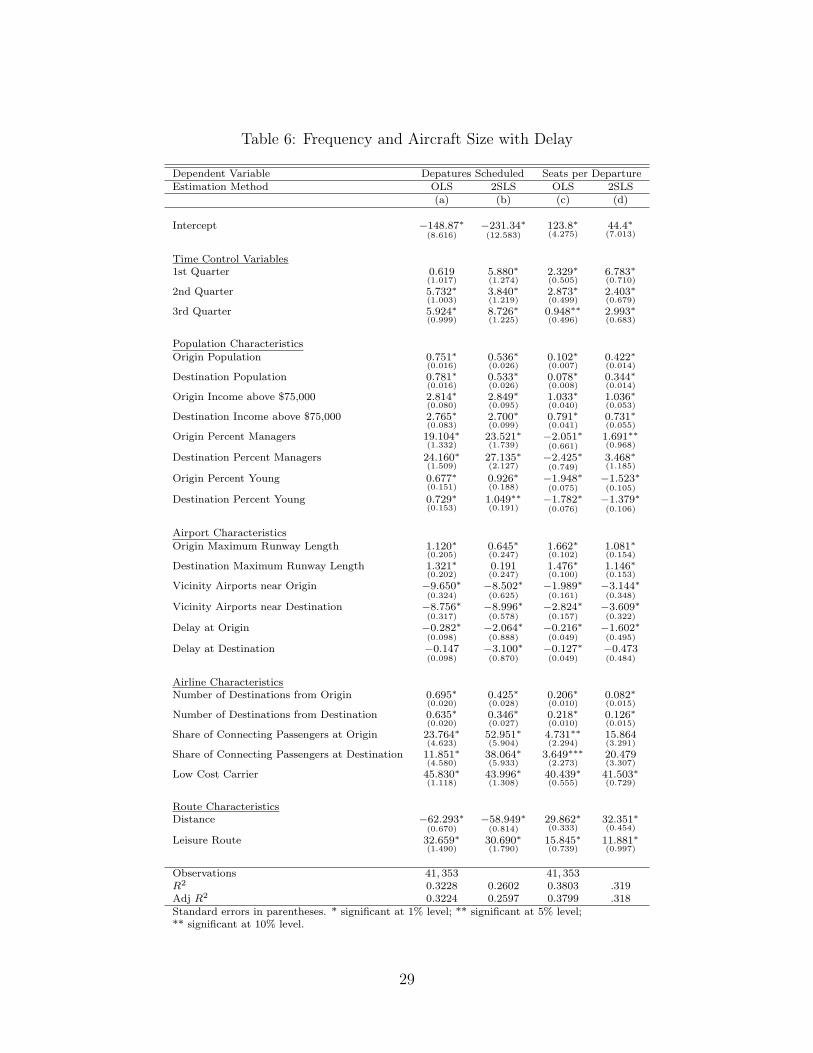
Table 6: Frequency and Aircraft Size with Delay

Dependent Variable Depatures Scheduled Seats per DepartureEstimation Method OLS 2SLS OLS 2SLS

(a) (b) (c) (d)

Intercept −148.87∗(8.616)

−231.34∗(12.583)

123.8∗(4.275)

44.4∗(7.013)

Time Control Variables1st Quarter 0.619

(1.017)5.880∗(1.274)

2.329∗(0.505)

6.783∗(0.710)

2nd Quarter 5.732∗(1.003)

3.840∗(1.219)

2.873∗(0.499)

2.403∗(0.679)

3rd Quarter 5.924∗(0.999)

8.726∗(1.225)

0.948∗∗(0.496)

2.993∗(0.683)



0.536∗(0.026)

0.102∗(0.007)

0.422∗(0.014)


0.533∗(0.026)

0.078∗(0.008)

0.344∗(0.014)


2.849∗(0.095)

1.033∗(0.040)

1.036∗(0.053)


2.700∗(0.099)

0.791∗(0.041)

0.731∗(0.055)


23.521∗(1.739)

−2.051∗(0.661)

1.691∗∗(0.968)


27.135∗(2.127)

−2.425∗(0.749)

3.468∗(1.185)

Origin Percent Young 0.677∗(0.151)

0.926∗(0.188)

−1.948∗(0.075)

−1.523∗(0.105)

Destination Percent Young 0.729∗(0.153)

1.049∗∗(0.191)

−1.782∗(0.076)

−1.379∗(0.106)



0.645∗(0.247)

1.662∗(0.102)

1.081∗(0.154)


0.191(0.247)

1.476∗(0.100)

1.146∗(0.153)


−8.502∗(0.625)

−1.989∗(0.161)

−3.144∗(0.348)


−8.996∗(0.578)

−2.824∗(0.157)

−3.609∗(0.322)

Delay at Origin −0.282∗(0.098)

−2.064∗(0.888)

−0.216∗(0.049)

−1.602∗(0.495)

Delay at Destination −0.147(0.098)

−3.100∗(0.870)

−0.127∗(0.049)

−0.473(0.484)


(0.020)0.425∗(0.028)

0.206∗(0.010)

0.082∗(0.015)


0.346∗(0.027)

0.218∗(0.010)

0.126∗(0.015)


52.951∗(5.904)

4.731∗∗(2.294)

15.864(3.291)


38.064∗(5.933)

3.649∗∗∗(2.273)

20.479(3.307)


43.996∗(1.308)

40.439∗(0.555)

41.503∗(0.729)


(0.670)−58.949∗

(0.814)29.862∗(0.333)

32.351∗(0.454)


30.690∗(1.790)

15.845∗(0.739)

11.881∗(0.997)

Observations 41, 353 41, 353R2 0.3228 0.2602 0.3803 .319Adj R2 0.3224 0.2597 0.3799 .318Standard errors in parentheses. * significant at 1% level; ** significant at 5% level;** significant at 10% level.

29

Table 7: Frequency and Aircraft Size with Cancellations

Dependent Variable Departures Scheduled Seats per DepartureEstimation Method OLS 2SLS OLS 2SLS

(a) (b) (c) (d)

Intercept −164.66∗(8.544)

−128.48∗(19.316)

113.19∗(4.256)

112.44∗(9.350)

Time Control Variables1st Quarter −0.620

(0.996)−21.118∗

(2.640)2.610∗(0.506)

−6.245∗(0.797)

2nd Quarter 6.618∗(0.985)

13.214∗(2.292)

2.897∗(0.500)

6.601∗(1.109)

3rd Quarter 3.115∗(0.982)

22.394∗(2.806)

0.690(0.499)

−11.206∗(1.358)



0.239∗(0.045)

0.080∗(0.008)

0.010(0.022)


0.270∗(0.045)

0.058∗(0.008)

−0.103(0.0223)


1.306∗(0.195)

1.015∗(0.040)

0.340∗(0.094)


1.239∗(0.201)

0.767∗(0.041)

0.089(0.097)


13.740∗(2.844)

−1.541∗(0.661)

−2.242∗∗∗(1.370)


18.308∗(3.242)

−1.671∗∗(0.742)

−2.120(1.560)

Origin Percent Young 0.995∗(0.148)

2.705∗(0.367)

−1.860∗(0.075)

−0.883∗(0.178)

Destination Percent Young 1.056∗(0.151)

2.982∗(0.375)

−1.686∗(0.076)

−0.655∗(0.181)



1.008∗(0.463)

1.520∗(0.102)

0.945∗(0.224)


0.126(0.454)

1.367∗(0.100)

0.974∗(0.220)


−3.026∗(0.832)

−2.047∗(0.159)

−0.314(0.403)


−2.607∗(0.797)

−2.876∗(0.156)

−1.130∗(0.386)

Cancellations at Origin 0.057∗(0.002)

0.552∗(0.056)

0.009∗(0.001)

0.286∗(0.027)

Cancellations at Destination 0.056∗(0.002)

0.541∗(0.045)

0.009∗(0.001)

0.197∗(0.022)


(0.020)−1.355∗(0.144)

0.155∗(0.010)

−0.548∗(0.070)


−1.277∗(0.151)

0.173∗(0.010)

−0.654∗(0.073)


69.431∗(10.535)

7.854∗(2.296)

23.285∗(5.102)


42.518∗(10.190)

7.183∗(2.273)

12.686∗(4.934)


7.663∗(3.159)

40.050∗(0.558)

25.307∗(1.530)


(0.663)−26.246∗

(2.567)30.675∗(0.336)

46.080∗(1.243)


31.724∗(3.209)

15.369∗(0.741)

13.374∗(1.554)

Observations 41, 353 41, 353R2 0.348 .319 0.346 0.143Adj R2 0.347 .318 0.346 0.142Standard errors in parentheses. * significant at 1% level; ** significant at 5% level;*** significant at 10% level

30

References

[1] Babikian, R., Lukacho, S.P., Waitz, I.A. (2002) The historical fuel efficiency characteristicsof regional aircraft from technological, operational, and cost perspectives. Journal of AirTransport Management 8, 389-400.

[2] Bhadra, D. (2005), Choice of Aircraft Fleets in the U.S. Domestic Scheduled Air Trans-portation System: Findings from a Multinomial Logit Analysis, Journal of the Trans-portation Research Forum, Fall 2005

[3] Brueckner, J.K (2004). Network structure and airline scheduling. Journal of IndustrialEconomics 52, 291-311.

[4] Brueckner, J.K, and Flores-Fillol, R (2007). Airline Schedule Competition. Review ofIndustrial Organization, 30, 161-177

[5] Brueckner, J.K, and Pai, V (2007). Technological Innovation in the Airline Industry:The Impact of Regional Jets. Department of Economics Working Paper, University ofCalifornia, Irvine.

[6] Dresner, M., Windle, R., Zhou, M. (2002a). Regional jet services: supply and demand.Journal of Air Transport Management 8, 267-273

[7] Dresner M., Windle, R., Zhou, M. (2002b). Airport barriers to entry in the US. Journalof Transport Economics and Policy, 36, 389-405.

[8] Forbes, S.J., Lederman, M. (2005). Control rights, network structure and vertical integra-tion: Evidence from regional airlines. Unpublished paper, University of California, SanDiego.

[9] Rupp, N.G. (2005). Flight Delays and Cancellations. Department of Economics WorkingPaper, East Carolina University

[10] Rupp, N., Holmes, G.M., (2007). An Investigation Into the Determinants of Flight Can-cellations. Forthcomming, Economica

[11] Wei W. and Hansen M. (2003) Cost economics of aircraft size. Journal of TransportEconomics and Policy, 37, 279-296.

31

6 Appendix

6.1 Census

Demographic data for this analysis comes from the 2000 Census data gathered from the 2007State and Metropolitan databook. Airports were assigned to a metropolitan statistical area(MSA) based on the name of the airport. Most airports identify themselves as serving a specificcity, and therefore a matching MSA, making the assignment of census data unambiguous.However, ambiguity arises in two special cases: (i) where one airport serves multiple MSAs,and (ii) where multiple airports serve a given MSA.

In case (i), the population-weighted average of the demographic data for the relevant MSAswas computed. Affected airports were CAK, where the Akron, OH and Canton-Massillon, OHMSAs were combined; ELM, where the Corning, NY and Elmira, NY MSAs were combined;MAF, where the Midland, TX and Odessa, TX MSAs were combined; RDU, where the Raleighand Durham, NC MSAs were combined. For the Hartford-Springfield International Airport,BDL, the airport was assigned to the Hartford, CT, MSA due to the longer distance to Spring-field, MA.

In case (ii), the same MSA was assigned to each airport in the area, unless it was possible toassign a Metropolitan Division to the airport. For the Los Angeles MSA, Los Angeles Interna-tional (LAX) was assigned to the Los Angeles Metropolitan Division and Orange County JohnWayne (SNA) to the Santa Ana-Anaheim-Irvine Division. For the San Francisco Bay Area,San Francisco International (SFO) was assigned to the San Francisco-San Mateo-RedwoodCity Division, and Oakland International (OAK) to the Oakland-Fremont-Hayward Division.San Jose Mineta International (SJC) was assigned to the San Jose-Sunnyvale-Santa Clara,CA MSA. In the Chicago area, O’Hare (ORD) and Midway (MDW) were assigned to theChicago MSA. For the New York City area, LaGuardia (LGA), John F. Kennedy (JFK), andNewark (EWR) were assigned to the New York-North New Jersey-Long Island MSA. Islip(ISP) and White Plains (HPN) were assigned to the Nassau-Suffolk and New York-WhitePlains Metropolitan Divisions respectively.

Several airports do not fall into a MSA or could not be easily assigned to a MetropolitanDivision in a large MSA, and for these cases, census data were gathered for the city in whichairport is located. These airports are Traverse City, MI, Pasco, WA, Montrose, CO, Missoula,MT, Melbourne, FL, Jackson, WY, Helena, MT, Gunnison, CO, Bozeman, MT, Vail, CO,Kailspell, MT, Meridian, MS, Butte, MT, Hanover, NH Minot, ND, Harlingen, TX, Temple,TX, Cody, WY, Burbank, CA, Long Beach, CA, Palm Springs, CA, Aspen, CO, Durango,CO, Hayden, CO, KeyWest, FL,Marathon, FL, Brunswick, GA, Burlington, IA, Presque Isle,ME, Nantucket, MA. Due to the lack of available data, Martha’s Vineyard and Hyannis, MAwere assigned to their respective counties of Barnstable and Dukes.

32

6.2 Hub Cities via Number of Destinations and ConnectingShare

Table 8: Hub Cities for Network Carriers

Major Airport Number of Destinations Share of Connecting PassengersAmerican Dallas-Ft. Worth (DFW) 126 0.47684

Chicago O’Hare (ORD) 99 0.33761St. Louis (STL) 66 0.23641Miami (MIA) 38 0.12158Los Angeles Int’l (LAX) 24 0.14046New York LaGuardia (LGA) 24 0.03106Boston (BOS) 21 0.02420Raleigh-Durham (RDU) 14 0.02580New York JFK (JFK) 11 0.04009Washington National (DCA) 9 0.03656Memphis (BNA) 9 0.02662

Alaska Seattle (SEA) 44 0.20299Portland (PDX) 28 0.15554Denver (DEN) 16 0.27356Los Angeles Int’l (LAX) 11 0.09976Boise (BOI) 10 0.12585Spokane (GEG) 5 0.02234San Francisco (SFO) 4 0.11657Sacramento (SMF) 4 0.04206San Jose (SJC) 4 0.03367Palm Springs (PSP) 4 0.00719

33

Major Airport Number of Destinations Share of Connecting PassengersContinental Houston Bush Intercontinental (IAH) 119 0.40066

Newark (EWR) 76 0.08643Cleveland Hopkins (CLE) 74 0.23353Boston (BOS) 13 0.02228Albany (ALB) 10 0.03869Tampa (TPA) 6 0.05831Westchester Co, NY(HPN) 5 0.03186Ft Myers, FL (RSW) 5 0.01299Rochester (ROC) 4 0.06341Syracuse (SYR) 4 0.04728Ft Lauderdale (FLL) 4 0.03522Miami (MIA) 4 0.03451Burlington (BTV) 4 0.03013Baltimore (BWI) 4 0.02837Sarasota (SRQ) 4 0.01653Portland, ME (PWM) 4 0.01316

Delta Atlanta (ATL) 155 0.5202Cincinnati (CVG) 124 0.61452Salt Lake City (SLC) 78 0.36503Orlando (MCO) 48 0.05063Dallas-Ft. Worth (DFW) 38 0.05964New York JFK (JFK) 36 0.04308Ft Lauderdale (FLL) 25 0.01997Tampa (TPA) 24 0.03057Boston (BOS) 23 0.02281New York LaGuardia (LGA) 23 0.01859

Northwest Minneapolis-St Paul (MSP) 137 0.45065Detroit (DTW) 125 0.44509Memphis (MEM) 86 0.66343Indianapolis (IND) 20 0.06498Milwaukee (MKE) 15 0.05019Washington Reagan (DCA) 7 0.02163Las Angeles (LAX) 6 0.06247Las Vegas (LAS) 6 0.02272Orlando (MCO) 6 0.01729St Louis (STL) 5 0.03032Denver (DEN) 5 0.02807Tampa (TPA) 5 0.02695New York LaGaurdia (LGA) 5 0.02213Kansas City, MO (MCI) 5 0.02161Flint (FNT) 5 0.02037Ft Lauderdale (FLL) 5 0.01745Ft Myers, FL (RSW) 5 0.00769Boston (BOS) 5 0.00757

34

Major Airport Number of Destinations Share of Connecting PassengersUnited Chicago O’Hare (ORD) 110 0.35742

Denver (DEN) 88 0.40310Washington Dullas (IAD) 64 0.19418San Francisco (SFO) 44 0.20823Los Angeles Int’l (LAX) 40 0.21023Salt Lake City (SLC) 14 0.67047Portland, OR (PDX) 10 0.07273Seattle (SEA) 8 0.05637Las Vegas (LAS) 7 0.10675Phoenix (PHX) 6 0.17216San Diego (SAN) 6 0.04188Sacramento (SMF) 6 0.03936

US Airways Charlotte (CLT) 93 0.62698Philadelphia (PHL) 81 0.27806Phoenix (PHX) 75 0.39992Pittsburgh (PIT) 62 0.22192Las Vegas (LAS) 57 0.18202Washington National (DCA) 47 0.18788New York LaGuardia (LGA) 36 0.09671Boston (BOS) 27 0.02319Hartford (BDL) 25 0.01202Syracuse (SYR) 24 0.01702

Major Airport Number of Destinations Share of Connecting PassengersJetblue New York JFK (JFK) 24 0.06719

Boston (BOS) 12 0.00060Long Beach (LGB) 7 0.01338Ft Lauderdale (FLL) 6 0.00086Washington Dulles (IAD) 5 0.00610Oakland (OAK) 4 0.00280West Palm Beach (PBI) 4 0.00019Las Vegas (LAS) 3 0.00683Orlando (MCO) 3 0.00014Tampa (TPA) 3 0.00008Ft Myers (RSW) 3 0

AirTran Atlanta (ATL) 46 0.39972Orlando (MCO) 17 0.00083Baltimore (BWI) 11 0.06214Tampa (TPA) 11 0.00068Philadelphia (PHL) 8 0.01565Ft Lauderdale (FLL) 7 0.00035Dallas-Ft Worth (DFW) 6 0.01531Boston (BOS) 6 0.00100Ft Myers (RSW) 6 0.00063Akron/Canton (CAK) 5 0.00956Hampton, VA (PHF) 5 0.00718Chicago Midway (MDW) 5 0.00634Rochester (ROC) 5 0.00036Sarasota, FL (SRQ) 5 0.00035

35

Major Airport Number of Destinations Share of Connecting PassengersATA Chicago Midway (MDW) 26 0.25645

Indianapolis (IND) 16 0.00700Phoenix (PHX) 3 0.23817Las Vegas (LAS) 2 0.09120Denver (DEN) 2 0.05906Orlando (MCO) 2 0.04029Dallas-Ft Forth (DFW) 2 0.02928Las Angeles (LAX) 2 0.01896New York LaGaurdia (LGA) 2 0.01379Ft Myers, FL (RSW) 2 0.00161

Southwest Las Vegas (LAS) 49 0.26799Chicago Midway (MDW) 42 0.27708Phoenix (PHX) 39 0.26699Baltimore (BWI) 34 0.24998Nashville (BNA) 27 0.25068Orlando (MCO) 27 0.12897Houston (HOU) 26 0.29152Tampa (TPA) 25 0.13348St Louis (STL) 21 0.20217Albuquerque (ABQ) 21 0.16704Los Angeles Intl (LAX) 21 0.11423Oakland (OAK) 20 0.06930Kansas City, MO (MCI) 19 0.16761

36

Documents

On the Factors that A ect Airline Flight Frequency and ... · PDF fileOn the Factors that A ect Airline Flight Frequency and Aircraft Size Vivek Pai ... force or the proportion of