Flight Frequency and Mergers

in Airline Markets

Oliver Richard∗

July 2002

Abstract

The welfare consequences of airline mergers have been analyzed almostexclusively in terms of ticket price. However, when flight frequency deci-sions are endogenized in a model, we can estimate measures of the relativeimportance of price and flight frequency in customer decisions. Hence, ina merger analysis, we can not only predict changes in flight frequency, butalso the consequences of those changes on consumer welfare. In this paper,merger simulations suggest that while passenger volume and consumer sur-plus decrease on the aggregate, some markets benefit from welfare gains oncemerger-induced changes in flight frequency are factored in.

Keywords: Structural Estimation, Airline Industry, Flight Frequency,Consumer Welfare, Mergers

JEL Classifications: L11, C31, C51, L93

∗ Simon School of Business, University of Rochester, Rochester, NY 14627; E-mail:

richard@ssb.rochester.edu. I am most grateful to the editor and two anonymous referees for the qualiy

of their comments. I also want to thank Olivier Armantier, Pamela Bedore, David Genesove, Jean-

Francois Richard, Ron Schmidt, and Greg Shaffer for helpful comments and suggestions. I thank

seminar participants at various universities and at the Econometric Society World Congress.

1. Introduction

Studies of airline mergers have focused almost exclusively on ticket price when determin-

ing consumer welfare, often suggesting that because mergers tend to raise ticket prices,

consumers are harmed (e.g. Borenstein (1990), Kim and Singal (1993)).1 This approach,

however, is based on the notion that consumers value only price and omits additional

considerations that affect consumer choices, such as flight frequency. Indeed, consumers

value the convenience of a flight schedule with multiple departure times, because they

are then more able to find a flight that is closer to their desired departure time. To

jointly incorporate valuation of ticket price and flight frequency requires a model with

endogenous flight decisions, which this paper provides and estimates on a sample of U.S.

markets.2 Hence, I can predict not only changes in flight frequency in a merger, but also

the relative consequences of those changes on consumer welfare.

I find that even though the net consumer surplus, as it relates to passengers on

nonstop flights, falls by 20% on average following a merger, it increases in 11% of the

sample markets. In those markets, consumers benefit despite the reduced competition,

once increases in flight frequency following the merger are factored in, a result that

derives from the comprehensiveness of the model. The importance of getting a full

1See, as well, Werden, Joskow, and Johnson (1991), Brueckner, Dyer and Spiller (1992), Morrison(1996), and the U.S. General Accounting Office (e.g. GAO/RCED90-102, Washington D.C.) for insighfuldiscussions of fare changes, using hedonic regressions on pre- and post-merger ticket prices. Topicsreviewed include TWA’s purchase of Ozark Airlines, and the Northwest/Republic Airlines and USAirways/Piedmont Airlines mergers in 1985-1988. Papers by Brueckner (2001) and Bamberger, Carltonand Neuman (2000) provide valuable insights on price changes in airline alliances during the 1990’s.

2While the empirical work of Berry (1990), Morrison and Winston (1995), and Berry, Carnall, andSpiller (1997) provides interesting structural models where several factors are considered in consumerdecisions, these do not endogenize airlines’ frequency decisions.

2

picture of consumer welfare is particularly clear in the airline industry, where policy

makers now consider consumer welfare the deciding factor in antitrust cases.

The paper is structured as follows. Section 2 introduces the model and Section 3

describes the application and data. Section 4 outlines the functional forms and estima-

tion methodology. Section 5 discusses the estimation results. Section 6 analyzes the

consumer welfare consequences of hypothetical mergers. Section 7 concludes.

2. A Model of Firms’ Decisions

Consider a market with two airlines (i = 1, 2) with nonstop flights (hereafter flights),

where a market is defined as a pair of U.S. airports without reference to an origin and

destination. For example, the pairs of airports Miami-Chicago O’Hare and Chicago

O’Hare-Miami are the same market. In the market, let fi be airline i’s number of flights

(or flight frequency); qi be the number of tickets sold by airline i (i.e., its passenger

volume); and pi be the airline’s ticket price. Finally, let q0 be the numeraire good; that

is, a composite good that represent all commodities other than those under consideration.

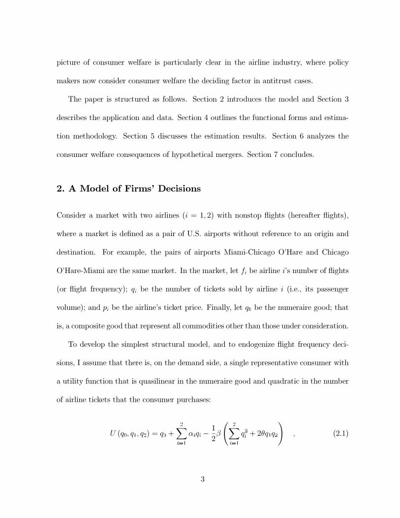
To develop the simplest structural model, and to endogenize flight frequency deci-

sions, I assume that there is, on the demand side, a single representative consumer with

a utility function that is quasilinear in the numeraire good and quadratic in the number

of airline tickets that the consumer purchases:

U (q0, q1, q2) = q0 +2∑

i=1

αiqi −1

2β

(2∑

i=1

q2i+ 2θq1q2

), (2.1)

3

where αi, β and θ are parameters, with αi, β ≥ 0 and −1 ≤ θ ≤ 1.3 In (2.1), airline

products may be imperfect substitutes and, to the extent that the valuation parameters

αi differ across airlines, the consumer may prefer one brand to the other.

The effective price of airline i’s good to the consumer is assumed to be additively

separable in the airline’s ticket price and the consumer’s cost of schedule delay with

airline i. Following Douglas and Miller (1972), this cost represents the dollar value

of the time difference between the consumer’s desired departure time and the closest

scheduled departure time on airline i. This time difference is specified as inversely

proportional to airline i’s flight frequency. I assume that airline i’s effective price, Pi, is

equal to pi+γ√fi, where γ is a parameter and γ√

fiis the consumer’s cost of schedule delay

on airline i.4 Airline models with effective prices include, among others, Panzar (1979),

Lederer (1993), Morrison and Winston (1995), and Brueckner and Zhang (2001).5

The representative consumer maximizes U (q0, q1, q2)− q0 −∑

2

i=1 Piqi, and this op-

3The model may be modified to include many consumers of the same type with utility as in (2.1).For example, to include K consumers while maintaining aggregate output of product i at qi (i.e. eachconsumer ultimately buys qi/K), we may rescale β to βK in (2.1) and write airline i’s profits in (2.3)

as∑K

k=1 (pi − ci,q) qi,k − ci,f fi, where qi,k is the quantity of product i purchased by consumer k. Thefirst-order conditions are comparable to (2.4)-(2.5), and the welfare analysis in my paper is unchanged.

4If flights are located at equal time intervals (along the 24-hr circle) and desired departure times areuniformly distributed, then the distance from the closest scheduled departure time on airline i is onaverage proportional to 1

fi. However, as Borenstein and Netz (1999) remark, an airline actually groups

some of its departure times, so that a specification of 1√fi, which is less convex in the flight frequency,

is more appropriate. Empirically, a square root specification yields a better fit than a linear one.5Alternative interpretations of the cost of schedule delay have been offered in the literature. For

instance, a consumer may be willing to pay a higher price for an airline with multiple daily flights sincehe knows he gets priority seating on another flight of this airline should his original flight be cancelled.The consumer may also value frequent flyer miles, in which case a schedule with a higher number ofdaily flights affords the consumer greater flexibility in future travel plans. Note that Panzar (1979),Lederer (1993) and Brueckner and Zhang (2001) are theoretical analyses of location of flight departuretimes, while Morrison and Winston (1995) provide an in-depth empirical overview of the industry.

4

timization problem yields the following system of linear inverse demand functions:

Pi = αi − βqi − βθq−i i = 1, 2 , (2.2)

where goods are substitutes, independent, or complements according to θ � 0.

Following Reiss and Spiller (1989), Brander and Zhang (1990) and Hendricks, Pic-

cione, and Tan (1997), I assume that airlines have constant marginal costs. Let ci,q

denote airline i’s marginal cost per passenger and ci,f be its marginal cost per flight.

The two airlines simultaneously maximize profits by selecting their number of flights

and of passengers for these flights. In other words, firm i maximizes its profits by

selecting a flight frequency f ∗i and a quantity q∗i such that:

(q∗i , f∗

i ) = Argmaxqi,fi

(pi − ci,q) qi − ci,f fi

= Argmaxqi,fi

(αi − βqi − βθq

−i − γ√fi

− ci,q

)qi − ci,f fi . (2.3)

The first-order conditions (hereafter FOC) to the problem in (2.3) are:

γqi2fi

√fi

− ci,f = 0 , (2.4)

αi − 2βqi − βθq−i − γ√

fi− ci,q = 0 i = 1, 2 , (2.5)

where equation (2.4) is the FOC with respect to fi and (2.5) is the FOC with respect to

5

qi. Substituting (2.4) in (2.5), I obtain that:

αi − 2βqi − βθq−i = ci,q +

γ2/3(2ci,f)1/3

q1/3i

. (2.6)

Equation (2.6) shows that the model may be re-interpreted in terms of economies of den-

sity; that is, all else equal, the marginal cost per passenger (here, a composite of airline

and consumer costs) decreases with the number of passengers. Such specifications are

common to the airline literature (see Caves, Christensen, Tretheway (1984), Brueckner

and Spiller (1991, 1994), Berry, Carnall and Spiller (1997)) and are typically introduced

from cost-based conjectures.6 My model highlights that such economies may likewise

obtain from a consumer’s valuation of time delays. In other words, there are economies

of schedule delay, indexed by the parameter γ, on the demand side.

3. An Application

3.1. American Airlines and United Airlines at Chicago O’Hare

In this paper, I examine the decisions of American Airlines (hereafter AA) and United

Airlines (UA) in markets at Chicago O’Hare airport (ORD). I justify the maintained

hypotheses of Section 2’s model according to the following facts:

(i) At O’Hare, AA and UA are in duopoly competition, as assumed by Brander and

Zhang (1990, 1993). This airport is a major hub for AA and UA. These two airlines

6The traditional conjecture is that a larger passenger volume can be accomodated with larger aircraftwhich have a lower cost per passenger. See Brueckner and Spiller (1991, 1994) and Brueckner (2001)for interesting applications of this concept to the analysis of, respectively, airline mergers and alliances.

6

jointly account for 90% of passenger enplanements at O’Hare and, together, they are

present on all of approximately 125 active markets at the airport. By comparison, Delta

Airlines, the third largest airline at O’Hare, has only 3.1% of passenger enplanements

and offers flights on just 8 markets. In this context, the implicit hypothesis that there

are no substitutes competing with flights offered by AA and UA over the sample hub

markets is reasonable.7

(ii) The internal structure of airline companies is such that Marketing and Fleet As-

signment Groups at the airlines first simultaneously determine the aggregate number of

passengers and flights on each of the sample markets. In practice, changes in aggregated

quantities and flights are rare and costly, while price fluctuations are numerous. This

is reasonably consistent with a Cournot model where firms commit to quantities and

then prices adjust along the reaction curves. The Cournot assumption is common to

most empirical studies on the airline industry (e.g. Reiss and Spiller (1989), Armantier

and Richard (2002)). In addition, Brander and Zhang (1990) find empirical support for

the hypothesis of Cournot competition between AA and UA at Chicago O’Hare. My

model remains nevertheless a simplification of airline behavior as I do not consider, for

instance, capacity choices and issues of aircraft landing and take-off slots at O’Hare.

7The inclusion of potential substitutes would require that I consider every airport and every airlinewith flights with one or more stops, as well as other means of transportation. Such an analysis is beyondthe scope of this paper.

7

3.2. Data

I have monthly passenger, frequency, and cost data for the year 1993. The Databank

28DS T-100, maintained by the U.S. Department of Transportation, reports the monthly

number of nonstop flights and passengers per market and per major airline. It indicates

the mix of aircraft types used, but it provides no flight scheduling information. The

Aircraft Operating Costs and Statistics, from AVMARK Inc., provide network-wide

operating costs per type of jet aircraft and per major airline. As airlines primarily

base aircraft assignment on mileage and network-wide routing, I assume that the mix

of aircraft types used in a market is invariant to frequency choices. I then combine the

aircraft data in the two databases to create airline cost variables.8

The sample data consist of duopoly (i.e. AA and UA) markets with Chicago-O’Hare

and each of 26 different U.S. airports, across each of the 12 months of 1993. There are

thus 312 markets with two airlines in the sample data for a total 624 airline observations.

The non-O’Hare airports are in large metropolitan areas (e.g. New York, San Diego),

in hub cities of AA and UA (e.g. San Francisco, Nashville), and in midsize Midwestern

and Eastern metropolitan areas that feed into AA and UA’s O’Hare hub (e.g. Rochester

(NY), Grand Rapids (MI)).9 A complete listing of the sample markets is provided in

8Since markets are defined as non-directional, the quantity and frequency values in a market are cal-culated by averaging values across both directions in the market (e.g. O’Hare-Rochester and Rochester-O’Hare). Values for the cost variables are computed as a weighted average across the types of aircraftused each month between two airports. The cost data are for the first quarter of 1993 and figures arethen adjusted to yield monthly data based on the monthly index for the cost of jet fuel. Note that thesource of the cost data is the Form 41 database, maintained by the U.S. Department of Transportation.

9Subsidiaries of AA and UA are associated with their parent company. Some subsidiaries at O’Haredo not report to Databank 28DS T-100. Markets with these airlines are identified using the OfficialAirline Guides and they are excluded from the sample due to lack of data.

8

Appendix 1 and descriptive sample statistics are provided in Table 1.

[Table 1 here]

4. Estimation of the Model of Firms’ Decisions

I propose to estimate the system of first-order conditions (2.4)-(2.5). As I do not observe

the firms’ marginal costs or demand functions, I specify in this Section their functional

forms and I outline the estimation methodology.

4.1. Functional Forms

Given the monthly data, the decision variables in Section 2’s model (i.e. flight frequency,

quantity) are defined on a monthly basis. I index the sample markets by the subscript

t, where t = 1, ..., 312, so that fi,t represents airline i’s number of flights (or flight

frequency) in market t, and qi,t is its total number of tickets sold in that market (i.e. its

passenger volume).

Firm i’s marginal cost per flight in equation (2.4) is specified as follows:

ci,f,t = λ0,i + λ1MILESt + λ2COSTi,t + λ3FUELi,t + λ4CASMi,t

+λ5WINTERt + εi,f,t i = AA,UA, t = 1, .., 312, (4.1)

where εi,f,t is the error term, λ0,i, ..., λ5 are the parameters, and λ0,i (i.e. the intercept)

is specific to each airline to account for fixed unobserved differences in frequency costs

across airlines. MILESt is the mileage between the airports in the market. COSTi,t is

9

a measure of airline i’s crew and insurance operating costs, and FUELi,t is a measure

of its fuel costs. I expect positive coefficients on these variables. CASMi,t denotes the

operating cost per available seat-mile for airline i. As the cost per available seat-mile

is lower for larger aircraft and larger aircraft are more costly to fly, I expect a negative

coefficient for CASMi,t. WINTERt is a dummy variable equal to 1 for markets in the

months of November, December, January and February, and equal to 0 for all other

markets. This variable controls for weather-related fluctuations in frequency costs.10

The error term εi,f,t then accounts for residual unobserved idiosyncratic factors that

may affect costs in a market, such as high winds.

Firm i’s marginal cost per passenger in equation (2.5) is given by:

ci,q,t = ω0,i + ω1MILESt + ω2CASMi,t + εi,q,t i = AA,UA, t = 1, .., 312, (4.2)

where εi,q,t is the error term, ω0,i, ..., ω2 are the parameters, and ω0,i (i.e., the intercept)

is specific to each airline to account for fixed unobserved differences in passenger costs

across airlines. The marginal cost per passenger rises with the airline’s cost per available

seat-mile, and I expect a positive coefficient on CASMi,t in (4.2).

As a consumer’s dollar valuation of time delays is a function of her income, I specify

that the cost of schedule delay associated with airline i in market t is in fact equal to

γINCt√fi,t

, where INCt is the median household income at the non-Chicago metropolitan

area in the market (source: Census data for metropolitan areas, 1990). After substituting

10The WINTER variable was added following tests on the presence of fixed effects for individual

months. Within each of theWINTER and non-WINTERmonths, coefficients on the dummy variables

for individual months do not significantly differ from each other.

10

for the effective price in the inverse demand function for firm i in (2.2), the empirical

inverse demand function is written as follows:

pi,t = α0,i + α1MILESt + α2POPt + α3,iHUBi,t + α4INCt + α5MONTHt

−βqi,t − βθq−i,t − γINCt√

fi,t

+ εi,d,t i = AA,UA, t = 1, .., 312, (4.3)

where εi,d,t is the error term, and α0,i, ..., α5, β, θ, γ are the parameters. POPt is the

population of the non-Chicago metropolitan area in the market, and HUBi,t is equal

to the population of the non-Chicago area if the non-ORD airport is also a major hub

for airline i. In the sample, these airports are Nashville and Raleigh-Durham for AA,

and San Franscico, Seattle and Washington D.C. for UA. MONTHt is defined, in each

sample month, as the sum of AA and UA’s average number of passengers in that month

in U.S. markets (other than the markets in the sample) with flights during all twelve

months of 1993. This variable controls for monthly variations in consumer demand. The

error term εi,d,t accounts for unobserved residual idiosyncratic factors that may affect

demand in a market, such as conventions or special cultural events.

Hence, the consumer’s valuation for airline travel in (4.3) depends upon an airline-

specific dummy variable (i.e., the intercept α0,i is specific to each airline), unobserved fac-

tors (MONTHt, εi,d,t), and demographics of the market and its non-Chicago metropoli-

tan area (MILESt, POPt, INCt, and HUBi,t). Here, I recognize that larger, wealthier

metropolitan areas tend to be major administrative, financial, and economic centers,

and a consumer in these markets may have higher valuation for airline service. Markets

11

linking O’Hare to another hub airport of AA and UA may also be more valuable to the

consumer, as they afford greater flexibility in travel opportunities beyond the market

itself. The range of these opportunities increases with the hub’s size, which is itself pro-

portional to the population of the city. This explains the variable HUBi,t in (4.3) and,

given the disparity in the size of the non-O’Hare hub cities across airlines, the coefficient

of HUBi,t is airline-specific (i.e., parameter α3,i). Similarly, the consumer may value the

travel opportunities afforded by AA and UA’s hub networks at O’Hare. As these hub

networks are (essentially) invariant in 1993, their characteristics may be proxied for with

an airline-specific dummy variable in the demand intercept, as I have done in (4.3) (i.e.,

α0,i).11 These airline dummy variables may, as well, proxy for the consumer’s valuation

of AA and UA’s frequent flyer programs and related marketing devices (see Borenstein

(1990), Morrison and Winston (1995)).

Substituting the specifications (4.1)-(4.3) in the FOC (2.4)-(2.5), I obtain the follow-

ing system of equations: ∀ i = AA,UA, t = 1, .., 312,

γINCtqi,t

2fi,t√fi,t

− (λ0,i + λ1MILESt + λ2COSTi,t + λ3FUELi,t + λ4CASMi,t (4.4)

+λ5WINTERt + εi,f,t) = 0 ,

(α0,i − ω0,i) + (α1 − ω1)MILESt + α2POPt + α3,iHUBi,t + α4INCt + α5MONTHt

−ω2CASMi,t − 2βqi,t − βθq−i,t − γINCt√

fi,t+ (εi,d,t − εi,q,t) = 0 . (4.5)

11Indeed, we may consider adding to (4.3) characteristics of all adjacent markets at O’Hare, suchas average population and income at all non-O’Hare metropolitan areas accessible from O’Hare withnonstop flights. As AA and UA’s networks of markets at O’Hare do not vary in any significant fashionin 1993, adding these characteristics is equivalent to adding an airline dummy variable to (4.3).

12

The parameters of the system (4.4)-(4.5) can only be identified up to a constant of

proportionality, and the pairs of parameters (α0,i, ω0,i) and (α1, ω1) cannot be separately

identified. Hence, I propose to rewrite the FOC as follow: ∀ i = AA,UA, t = 1, .., 312,

INCtqi,t

2fi,t√fi,t

− (λ∗0,i + λ∗

1MILESt + λ∗

2COSTi,t + λ∗

3FUELi,t + λ∗

4CASMi,t

+λ∗5WINTERt + εi,f,t) = 0 , (4.6)

α∗0,i + α∗

1MILESt + α∗

2POPt + α∗

3,iHUBi,t + α∗4INCt + α∗

5MONTHt

−ω∗2CASMi,t − qi,t − θ

2q−i,t − γ∗INCt√

fi,t+ εi,dq,t = 0 , (4.7)

where λ∗k = 2λkγ, α∗j = (αj−ωj)

2βfor j = 0, 1, α∗k = αk

2βfor j ≥ 3, ω∗2 = ω2

2β, γ∗k = γ

2β, and

εi,dq,t=(εi,d,t-εi,q,t).The parameters in (4.6)-(4.7) can now be identified, and I assume

that the residual error terms εi,f,t and εi,dq,t have mean zero and are independent across

markets.12

4.2. Estimation Methodology

I estimate the parameters in equations (4.6)-(4.7) with the Nonlinear Three-Stage Least

Squares method (see Appendix 2 for details). The instrumental variables are the model’s

exogenous variables. I find no evidence of heteroskedasticity in the estimated residuals.

Given the estimated parameters, I compute predicted flight frequencies and passenger

quantities on a market by the bootstrap method using a random draw of 100 residuals.

12Having controlled for fixed monthly effects in (4.6) with the variable WINTERt, I tested for theinclusion of dummy variables for individual months in (4.7), which already includes the control variableMONTHt. The coefficients on these variables were not significantly different from 0 at a 10% level,and these variables were not included, for parsimony.

13

Estimation and prediction results are listed in Table 2.

[Table 2 roughly here]

5. Estimation Results

The range and moments of the predicted values match closely with the sample data (see

Table 2). In particular, correlations between observed and predicted flight frequencies

and passenger quantities are, respectively, 0.91 and 0.94. This attests to the goodness

of fit of the model and provides support for the specification choices.

The estimated value for the cost of schedule delay parameter γ∗ is positive and

significantly different from zero at a 1% level. In other words, the data suggest that the

airline consumer significantly values the convenience of a flight schedule with multiple

departure times. The second-order conditions to the firms’ optimization problem in (2.3)

require that 3qi,t

√fi,t > γ̂∗INCt for i = AA,UA (i.e. γ∗ = γ/2β). These conditions

hold for each airline across all sample markets at the estimated value for γ∗, providing

additional support for the model.

In the cost estimates, the cost per flight is found to increase with the mileage of the

market, with crew and insurance costs, and with fuel expenses (i.e., MILESt, COSTi,t,

FUELi,t). It is estimated to be lower in the winter months (i.e., WINTERt). This

may be due to lower industry-wide consumption of jet fuel in those months, as airlines

tend to scale back their flight schedules in the winter. The cost per flight is higher for

aircraft with a lower cost per available seat-mile (i.e., CASMi,t in (4.6) in Table 2). As

these aircraft are typically the larger ones, this finding is consistent with larger aircraft

14

being more expensive to fly. The marginal cost per passenger rises, however, with the

cost-per-passenger mile, as expected (i.e., CASMi,t in (4.7) in Table 2).

Finally, the demand estimates reveal that the customer’s valuation for airline travel

increases with the mileage of the market and with the presence of a second hub airport

in the market (i.e., coefficients on HUBAA,t and HUBUA,t are positive and significant

at 1%). AA and UA’s products are also found to be imperfect substitutes, as θ̂ = 0.51.

This estimate is both significantly different from 1 (i.e., perfect substitutes) and from 0

(i.e., independent products) at the 1% level.

6. Application to Merger and Welfare Analysis

I now quantify the effects of a merger among the two airlines on a market. My focus is

on examining the extent to which changes in flight frequency affect passenger volumes

and consumer welfare. I do not explore the incentives of firms to merge.13

I assume that the two airlines (i.e. AA and UA) on a market merge into a single

entity. The demand and costs for the new firm are, respectively, the higher demand and

lower costs of the two previous competitors. The new monopoly firm thus selects its

13See Perry and Porter (1985) for a discussion of firms’ incentives to merge in Cournot models withregards to changes in productive capacity.

15

optimal frequency, ft, and quantity of passengers, qt, according to the following FOC:

INCtqtft√ft

− mini=AA,UA

(λ̂∗

0,i + λ̂∗

1MILESt + λ̂

∗

2COSTi,t + λ̂

∗

3FUELi,t + λ̂

∗

4CASMi,t

+λ̂∗

5WINTERt + ε̂i,f,t) = 0 , (6.1)

maxi=AA,UA

(α̂∗

0,i + α̂∗

1MILESt + α̂∗

2POPt + α̂∗

3,iHUBi,t + α̂∗

4INCt + α̂∗

5MONTHt

−ω̂∗

2CASMi,t + ε̂i,dq,t)− qt − γ̂∗INCt√

ft= 0 , (6.2)

where λ̂∗

k, α̂∗

k, ω̂∗

k, γ̂∗ and ε̂i,f,t, ε̂i,dq,t are, respectively, the estimated parameter values and

residual values. Based on equations (6.1)-(6.2), I simulate the predicted frequency and

passenger quantity for the new firm. These predictions are computed by the bootstrap

method using the same residual draws as for the predictions in Table 2.14

I then calculate changes in the consumer surplus following the merger.15 In the model

of Section 2, the net consumer surplus in a duopoly is equal to:

CSd = CS (q0, q1, q2) = U (q0, q1, q2)− q0 −2∑i=1

Piqi =β

2

[(q1)

2 + 2θq1q2 + (q2)2],

where the second equality follows from (2.1) and (2.2). When firm 1 is, say, in a

monopoly, the net consumer surplus is given by CSm = CS (q0, q1, 0) . If CSm > CSd,

then consumers are said to benefit from the merger. Note that the change in flight fre-

quency in the merger affects consumer welfare indirectly by affecting chosen quantities

14In 67% of the simulations, there is a net gain in demand or costs for the new firm; i.e., if the newfirm’s costs in (6.1) are from AA, then the demand & cost term in (6.2) is from UA, and vice-versa.

15The numbers I provide subsequently are likely to be a lower bound on the true change as someconsumers may ultimately choose alternate means or paths of transportation.

16

through its impact on the effective price. The interpretation of a gain then implicitly as-

sumes that even though the monopolist may offer fewer total flights than the duopolists

combined, its flight schedule reduces the cost of schedule delay of the representative

consumer. This would be the case, for instance, if the two former airlines had similar

departure times for their flights. Indeed, the new airline would then have the flexibility

to match those times and add new ones, thus benefiting the consumer. Borenstein and

Netz (1999) show that competitive hub airlines, such as AA and UA at ORD, schedule

flight departures at similar times, and the interpretation of a gain in consumer surplus

is therefore reasonable. Prediction and welfare results are found in Table 3.

[Table 3 here]

I find that the monopolist offers a higher flight frequency than each of the two

previous competitors, individually, across all sample markets (see Table 3). Given that

the model is Cournot with linear demands and (essentially) non-increasing marginal

costs (see (2.6)), this result is expected.

Under the merger, the predicted passenger volume averages to 80% of the predicted

total passenger volume under a duopoly structure. To put that number in perspective,

note that when the cost of schedule delay parameter γ is equal to 0 (i.e., the number of

flights in a market does not affect demand), then the ratio of the equilibrium quantity

in a monopoly/merger to the total quantity in a duopoly is equal to:

qm1

qd1+ qd

2

=(2 + θ) (max {α1,α2} −min {c1,q, c2,q})

2 (α1 + α2 − c1,q − c2,q)≥ (2 + θ)

4. (6.3)

17

At the estimated value θ̂ = 0.51, the lower bound on the ratio in (6.3) is equal to 0.628.16

As γ̂∗ > 0, the monopolist achieves a greater reduction in the cost of schedule delay, and

the lower bound in the sample data (achieved in the Los Angeles and New York markets)

is slightly higher, at 65.3%. In that context, an average ratio of 80% suggests non-trivial

valuation of increases in flight frequency on the part of consumers across markets.

In fact, if the net consumer surplus decreases by 20% on average in a sample market,

it increases in 34 of the 312 markets by an average of 19%. These gains obtain in some

of the smaller sample markets (e.g. Harrisburg (PA), Syracuse (NY)) which benefit

most from increases in flight frequency, as the cost of schedule delay specification is

decreasing and convex in the flight frequency. In these markets, the consumer benefits

in a merger despite the reduced competition, once the reduction in the cost of schedule

delay following an increase in flight frequency is factored in, a result that derives from

the comprehensive scope of the model.

7. Conclusion

I have proposed an analysis that recognizes that the airline consumer values not only

ticket price, but also the convenience of a flight schedule with multiple departure times.

As my model endogenizes flight frequency decisions, I can then predict changes in flight

frequency and their effect on consumer welfare. The results from the structural esti-

mation suggest significant valuation of flight frequency on the part of consumers. The

16When γ = 0, optimal total quantity in the monopoly and duopoly are, respectively, equal toqm1

= (max {α1,α2} − min {c1,q, c2,q}) ÷ 2β and qd1+ qd

2= (α1 + α2 − c1,q − c2,q) ÷ (2 + θ)β. Setting

α1 = α2 and c1,q = c2,q, the ratio in (6.3) is equal to 0.628. This figure is meaningful in this paper asα1 ≈ α2 and c1,q ≈ c2,q at the estimated parameter values.

18

subsequent merger simulations reveal that, while passenger volume and consumer wel-

fare decrease on the aggregate, increases in flight frequency following the merger benefit

consumers in some of the smaller markets.

This analysis therefore suggests that consumers’ valuation of a convenient flight

schedule is an important issue that warrants greater focus in policy analyses of consumer

welfare. The structural estimation in this paper provides a valuable tool for quantifying,

with simulations, how mergers may affect frequency decisions and consumers. Although

the analysis here focuses only on flight frequency, extensions to models with additional

quality measures or passenger types would be worthwhile. An extension to a multi-

market model with entry would also make it possible to analyze how entry decisions at

hub airports may factor in. Our recent work (see Armantier and Richard (2002)) in the

context of exchanges of cost information provides a blueprint for a broader analysis of

this type.

19

20

8. Tables

Table 1. Descriptive Sample Statistics.

Mean Std. Dev. Minimum Maximum

Flight frequency i,t 172 88 78 511

Passenger quantity i,t 15771 11253 3408 66912

Total passenger quantity t 31543 19869 10602 103503

MILES t 862 547 137 1846

COST i,t (in $) 1213.53 239.85 836.89 2266.95

FUEL i,t (in $) 997.58 266.30 540.01 2100.80

CASM i,t (in $) 0.045 0.009 0.029 0.075

POP t 2238232 2113984 392928 8863052

HUB i,t 0.096 0.295 0.000 1.000

INC t (in $) 33216 5962 24442 48115

MONTH t 18837 1686 15760 21439

Note: The frequency and quantity values are reported on a one-way basis.

21

Table 2. Estimation and Prediction Results for the Sample Duopoly Markets.

Estimation results:

FOC for flight frequency: equation (4.6) FOC for passenger quantity: equation (4.7)

Variable Estimate Std. Error Variable Estimate Std. Error

CONSTAA 242.3 23.0 CONSTAA -10508 3025

CONSTUA 252.8 23.3 CONSTUA -9577 3039

MILES t 0.075 0.006 MILES t 1.160 0.550

COST i,t # 0.345 0.037 POP t 0.0043 0.0003

FUEL i,t 0.056 0.012 HUBAA,t 0.0082 0.0012

CASM i,t -4543 427.7 HUBUA,t 0.0033 0.0002

WINTER t -25.94 5.46 INC t 0.210 0.072

MONTH t 1.247 0.117

CASM i,t ## 85780 18300

γ * 3.203 1.018

θ 0.515 0.065

Prediction results:

Square root of flight frequency Passenger quantity

Observed Predicted Observed Predicted

Mean 12.79 12.47 Mean 15771 15220

Std. Error 2.92 2.62 Std. Error 11253 10946

Min 8.80 7.33 Min 3408 1198

Max 22.61 20.37 Max 66912 58326

Correlation ### = 0.908 Correlation ### = 0.945

Notes: All estimates are significantly different from zero at a 5% level. CONST denotes the intercept. The minimized criterion value for the Nonlinear Three-Stage Least Squares estimation is equal to 308. # To lessen multicolinearity, FUEL is subtracted from COST prior to the estimation, and the estimate I report for the coefficient on COST applies to the variable (COST-FUEL). ## I report the value for ω2, the coefficient on CASM in equation (4.2). The negative of ω2 enters in equation (4.7). ### Correlation between observed and predicted values.

Table 3. Merger (Monopoly) Predictions and Comparison to Predictions when Market is in a Duopoly.

Duopoly Monopoly Difference Ratio of Monopoly to Duopoly

Prediction results: Mean Mean Mean Mean Min Max

Square root( flight frequency i,t ) # 13.17 15.53 2.36 1.190 1.015 1.491

Flight frequency i,t ## 181.0 247.9 66.9

Total passenger quantity t 30440 23256 -7184 0.800 0.653 1.251

Consumer surplus t 0.800 0.537 1.456

# For duopoly: Highest predicted flight frequency value amongst the two competitors. ## Based on predicted values for the square root of flight frequency.

9. References

Armantier, O. and Richard, O., 2002, ‘Exchanges of Cost Information in the Airline

Industry’, Rand Journal of Economics, forthcoming.

Bamberger G., Carlton, D. and Neuman, L., ‘An Empirical Investigation of the

Competitive Effects of Domestic Airline Alliances’, NBER Working Paper #W8197.

Berry, S., 1990, ‘Airport Presence as Product Differentiation’, American Economic

Review, Papers and Proceedings, 80, 394-399.

Berry, S., Carnall, M. and Spiller, P., 1997, ‘Airline Hubs: Costs, Markups and the

Implications of Customer Heterogeneity’, NBER Working Paper #5561.

Borenstein, S., 1990, ‘Airline Mergers, Airport Dominance, and Market Power’,

American Economic Review, Papers and Proceedings, 80, 400-404.

Borenstein, S. and Netz, J, 1999, ‘Why do all flights leave at 8am? Competition and

Departure-time Differentiation in Airline Markets’, International Journal of Industrial

Organization, 17, 611-640.

Brander, J. and Zhang, A., 1990, ‘Market Conduct in the Airline Industry: An

Empirical Investigation’, Rand Journal of Economics, 21, 567-583.

Brueckner, J., 2001, ‘The Economics of International Codesharing: An Analysis of

Airline Alliances’, International Journal of Industrial Organization, 19, 1475-1498.

Brueckner, J., Dyer, N. and Spiller, P., 1992, ‘Fare Determination in Airline Hub-

and-Spoke Networks’, Rand Journal of Economics, 23, 309-333.

Brueckner, J. and Spiller, P., 1991, ‘Competition and Mergers in Airline Networks’,

International Journal of Industrial Organization, 9, 323-342.

Brueckner, J. and Spiller, P., 1994, ‘Economies of Traffic Density in the Deregulated

Airline Industry’, Journal of Law and Economics, 37, 379-415.

Brueckner, J. and Zhang, A., 2001, ‘A Model of Scheduling in Airline Networks:

How a Hub-and-Spoke System Affects Flight Frequency, Fares and Welfare’, Journal of

Transport Economics and Policy, 35, 195-222.

Caves, D., Christensen, L. and Tretheway, M., 1984, ‘Economies of Density versus

22

Economies of Scale: Why Trunk and Local Service Airline Costs Differ’, Rand Journal

of Economics, 15, 471-489.

Douglas, G. and Miller, J.C., III, 1972, Economic Regulation of Domestic Air Trans-

port: Theory and Policy, Washington, D.C.: Brookings Institution.

Gallant, A., 1986, Nonlinear Statistical Models, New York: John Wiley& Sons.

Hendricks, K., Piccione, M. and Tan, G., 1997, ‘Entry and Exit in Hub-Spoke Net-

works’, Rand Journal of Economics, 28, 291-303.

Kim, E.H., and Singal, V., 1993, ‘Mergers and Market Power: Evidence from the

Airline Industry’, American Economic Review, 83, 549-569.

Lederer, P., 1993, ‘A Competitive Network Design Problem with Pricing’, Trans-

portation Science, 27, 25-38.

Morrison, S., 1996, ‘Airline Mergers: A Longer View’, Journal of Transport Eco-

nomics and Policy, 30, 237-250.

Morrison, S. and Winston, C., 1995, The Evolution of the Airline Industry, Wash-

ington, D.C.: Brookings Institution.

Panzar, J., 1979, ‘Equilibrium and Welfare in Unregulated Airline Markets’, Ameri-

can Economic Review, Papers and Proceedings, 69, 92-95.

Perry, M. and Porter, R., 1985, ‘Oligopoly and the Incentive for Horizontal Merger’,

American Economic Review, 75, 219-227.

Reiss, P. and Spiller, P., 1989, ‘Competition and Entry in Small Airline Markets’,

Journal of Law and Economics, 32, 179-202.

Werden, G., Joskow, A. and Johnson, R., 1991, ‘The Effects of Mergers on Price

and Output: Two Case Studies from the Airline Industry’, Managerial and Decision

Economics, 12, 341-352.

23

10. Appendix 1

The non-ORD airports in the data are: Albany (NY), Buffalo (NY), Columbus (OH), Des

Moines (IN), Grand Rapids (MI), Harrisburg (PA), Hartford (CT), Kansas City (KS),

Los Angeles LAX (CA), Miami (FL), Nashville (TN), New Orleans (LA), New York

Laguardia (NY), Omaha (NE), Portland (OR), Providence (RI), Raleigh-Durham (NC),

Rochester (NY), San Diego (CA), San Francisco (CA), Seattle (WA), San Jose (CA), St

Louis (MO), Syracuse (NY), Tampa Bay (FL), and Washington National (D.C.).

11. Appendix 2

I estimate a system of four equations: one of equations (4.6)-(4.7) per airline. There

are restrictions on the parameters across the two equations (4.6) and the two equations

(4.7). Hence, in the estimation, I update the variance-covariance matrix of the residuals

as follows: Let ε̂AA,f , ε̂UA,f , ε̂AA,dq, ε̂UA,dq be the vectors of first-stage residuals, with

ε̂i,k′ =

(ε̂i,k,1 ... ε̂i,k,m ... ε̂i,k,312

)for i = AA,UA, k = f, dq,

V ar (ε̂i,k) =2∑

j=1

ε̂j,k′ε̂j,k /624 ,

Cov (ε̂i,k ε̂−i,k) =

(ε̂1,k −

312∑m=1

(ε̂1,k,m

)/312

)′(ε̂2,k −

312∑m=1

(ε̂2,k,m

)/312

)/312 ,

Cov (ε̂i,k, ε̂i,−k) =2∑

j=1

ε̂j,f′ε̂j,d /624 , Cov

(ε̂i,k, ε̂−i,−k

)=

2∑j=1

ε̂j,f′ε̂−j,d /624 ,

since∑

312

m=1

(ε̂AA,k,m + ε̂UA,k,m

)= 0.

24