On the Evolution and Impact of Mobile Botnets in Wireless

1536-1233 (c) 2015 IEEE. Personal use is permitted, but republication/redistribution requires IEEE permission. Seehttp://www.ieee.org/publications_standards/publications/rights/index.html for more information.

This article has been accepted for publication in a future issue of this journal, but has not been fully edited. Content may change prior to final publication. Citation information: DOI10.1109/TMC.2015.2492545, IEEE Transactions on Mobile Computing

1

On the Evolution and Impact of Mobile Botnetsin Wireless Networks

Zhuo Lu, Member, IEEE, Wenye Wang, Senior Member, IEEE, and Cliff Wang, Senior Member, IEEE

Abstract—A botnet in mobile networks is a collection of compromised nodes due to mobile malware, which are able to perform

coordinated attacks. Different from Internet botnets, mobile botnets do not need to propagate using centralized infrastructures, but can

keep compromising vulnerable nodes in close proximity and evolving organically via data forwarding. Such a distributed mechanism

relies heavily on node mobility as well as wireless links, therefore breaks down the underlying premise in existing epidemic modeling for

Internet botnets. In this paper, we adopt a stochastic approach to study the evolution and impact of mobile botnets. We find that node

mobility can be a trigger to botnet propagation storms: the average size (i.e., number of compromised nodes) of a botnet increases

quadratically over time if the mobility range that each node can reach exceeds a threshold; otherwise, the botnet can only contaminate

a limited number of nodes with average size always bounded above. This also reveals that mobile botnets can propagate at the fastest

rate of quadratic growth in size, which is substantially slower than the exponential growth of Internet botnets. To measure the denial-

of-service impact of a mobile botnet, we define a new metric, called last chipper time, which is the last time that service requests,

even partially, can still be processed on time as the botnet keeps propagating and launching attacks. The last chipper time is identified

to decrease at most on the order of 1/√

B, where B is the network bandwidth. This result reveals that although increasing network

bandwidth can help mobile services, it can, at the same time, indeed escalate the risk of services being disrupted by mobile botnets.

Index Terms—Mobile botnet, malware, proximity propagation, wireless networks, denial-of-service, modeling and evaluation.

F

1 INTRODUCTION

With the proliferation of smart handheld devices andthe exploded number of malware on mobile platforms,a mobile botnet [1], [2], which is a collection of com-promised (or infected) mobile nodes. that can performcoordinated attacks, no longer occurs in theory, butcomes into practice. For example, Ikee.B [3] in 2009 wasfound to include command and control logic to render anumber of infected iPhones under the control. In 2012,Symantec found a large botnet Android.Bmaster [4] inChina that had infected an estimate of hundreds of thou-sands of Android phones. As a result, mobile botnetshave already become one of the most serious securitythreats to today’s mobile networks and applications.

A mobile botnet can compromise vulnerable nodes bysending malware via centralized infrastructures (e.g., us-ing short and multimedia message services [1], [4], [5]).However, to eschew increasingly enhanced monitoringof cellular infrastructures, a stealthy way for propagationis to stay off the radar and spread to vulnerable nodesnearby, which has been adopted in existing malware,such as Mabir, Lansco and CPMC [6]. A challengingquestion is how botnets propagate via such proximity in-fection, especially how they behave in mobile networkscompared with their forerunners in the Internet.

• Zhuo Lu is with the Department of Computer Science, University ofMemphis. Email: [email protected].

• Wenye Wang is with the Department of Electrical and Computer Engi-neering, North Carolina State University. Email: [email protected].

• Cliff Wang is with Army Research Office, Research Triangle Park, NC.Email: [email protected].

An earlier version of the work was published in IEEE INFOCOM 2014. Theresearch in this paper was supported by NSF CNS-142315 and CNS-1018447.

Extensive works have investigated Internet malwarepropagation using epidemic modeling (e.g., [7], [8]),which presumes a condition that an infected node cancompromise other vulnerable nodes with equal prob-ability. A few studies [9], [10] have adapted epidemicmodeling to characterize mobile malware based on sim-plistic random movements, where the equal-probabilityassumption still holds. These prior efforts conclude thatusing proximity infection, malware can continue infect-ing more nodes without using infrastructures, therebyleading to severe epidemics. This result is also observedby a number of experiments [11]–[13]. Interestingly, how-ever, a recent paper [14] draws an opposite conclusionbased on simulations that proximity infection only af-fects a limited number of nodes and is far less concern-ing in urban environments where node susceptibility isrelatively low. These somewhat discrepant results maybe due to different system setups, such as transmissionrange and random mobility. Nonetheless, the primaryreason is still unclear. As a result, it is not yet fullyunderstood how proximity infection can cause a botnetpropagation storm and what the impact is in mobile networks.

In this paper, we are motivated to address this openquestion by considering a practical scenario with het-erogeneous mobility, in which nodes are more likelyto move around in certain areas. Such heterogeneityinevitably breaks the premise of equal-probability infec-tion used in existing epidemic modeling [9], [10]. Thus,we take a stochastic approach to study how a mobilebotnet evolves. In particular, we denote by S(t) the setof infected nodes in a mobile botnet at time t. The botnetoriginates from an initially infected node that starts tomove around and compromise nearby vulnerable nodes



2

at time 0. We are interested in how the botnet size |S(t)|(defined as the number of infected nodes in the botnet)increases over time t.

Our results reveal an interesting dichotomy of mobilebotnet propagation: the average size of a mobile botnetE|S(t)| either grows quadratically over time t or isalways bounded above. In particular, given node densityλ, wireless transmission range r, and mobility radius αthat is the maximum range that a node can reach, we findthat as long as λ(2α + r)2 exceeds a threshold, E|S(t)|is a quadratical function of t; otherwise, |S(t)| is finitealmost surely with eventual size |S(∞)| exponentiallydistributed. This means that with fixed network setups λand r, sufficient mobility (i.e., mobility radius α becomeslarge) can provoke mobile botnet propagation from lim-ited infection to epidemics. Therefore, our findings notonly serve as a bridge to connect two discrepant resultsin the literature, but also reveal that mobile botnetsvia proximity infection can propagate at the fastest rateof quadratic growth, which is much slower than theexponential growth of Internet botnets.

In order to measure the denial-of-service impact of amobile botnet with quadratic growth in size, we definelast chipper time, the last time moment that a requiredratio σ of service requests from mobile nodes to aservice center can still be processed on time, while thebotnet keeps propagating and attacking. We find thatthe last chipper time decreases at most on the order

of 1/√

B log 11−σ

, where B is the network bandwidth.

Based on this, we can quantitatively assess how increasingnetwork bandwidth induces the risk of botnets to disruptmobile services. For example, the bandwidth of currentcellular networks is expected to increase 10 times fromLTE to LTE advanced, a mobile botnet, in the fastest case,needs to propagate only one third (i.e., 1/

√10) of the

time that it spends in LTE to disrupt the same service inLTE advanced.

The remainder of this paper is organized as follows.In Section 2, we introduce preliminaries and models. InSections 3 and 4, we investigate how a mobile botnetevolves and what its impact is. In Section 5, we presentrelated work. Finally, we conclude in Section 6.

2 PRELIMINARIES AND MODELS

In this section, we first present the models used in thispaper, then formulate the research problem.

2.1 Network and Mobile Users

We consider a hybrid mobile network with two distincttypes of nodes: mobile nodes that are common usersmoving around in the network, and infrastructure nodesthat are base stations or access points to provide mobileservices to mobile nodes.

There are n mobile nodes distributed independentlyand uniformly on a torus surface Ω = [0,

√

nλ]2 for some

node density λ. Infrastructure nodes form square cells

in the network, as shown in Fig. 1(a). They have thewireless network interface that offers wireless access tomobile nodes. In addition, they are interconnected witheach other via high-speed wireline networks and are alsoconnected to a data service center that processes servicerequests from mobile nodes.

mobile nodes

moving around

malware-infected nodes

also moving around

Infrastructure

node

transmission

radius r

...

... ...

......

...

...

...

...

...

...

(a)

(b)

Fig. 1. Network architecture: infrastructure nodes and

mobile nodes.

Mobile nodes are able to communicate directly witheach other, and can also communicate with their nearestinfrastructure nodes for mobile services. As shown inFig. 1(b), the transmission ranges of mobile and infras-tructure nodes are the same and denoted by r. Thenetwork bandwidth B is shared among all mobile andinfrastructure nodes. Mobile nodes consist of legitimatenodes and malicious nodes that are compromised bymalware and attempt to infect other mobile nodes inthe network. Infrastructure nodes, on the other hand,are invulnerable to malware infection.

2.2 Mobile Malware and Botnet

When a mobile node is infected by malware, it may notbehave legitimately. Generally speaking, mobile malwareis malicious software on mobile platforms that attemptsto take control of a device and copy itself to othersusceptible devices, which is called malware propagation[1], [3]. More dangerously, if mobile nodes are infectedby the same malware, they can form a mobile botnet [2],[3] that is a collection of compromised mobile devicesunder the same control. Mobile botnets have alreadybeen found in practice, such as Ikee.B in 2009 [3] andAndroid.Bmaster in 2011 [4]. In essence, a mobile botnetcan be formed in the following two ways: (i) propaga-tion through infrastructures (malware sending its copiesusing short/multimedia message services or advertisingits applications (APPs) on mobile markets [1], [4], [5]),(ii) proximity infection (a compromised node sendingmalware to nearby nodes using peer-to-peer wirelesslinks [6], [14]).

Although botnet propagation is very fast throughinfrastructures, it can be easily ceased by increasingly en-hanced security systems at infrastructures (e.g., Google’s



3

Android kill switch). Hence, a stealthy and safe way forpropagation is to infect vulnerable nodes nearby, becausesuch proximity infection can easily persist and remainundetected due to the nature of decentralized infectionand the dynamic network topology. The proximity in-fection mechanism has already been found in existingmalware, such as Mabir, Lansco and CPMC [6].

mobility trac

e

infected node

susceptiblesusceptible

infected infected

…

…

…

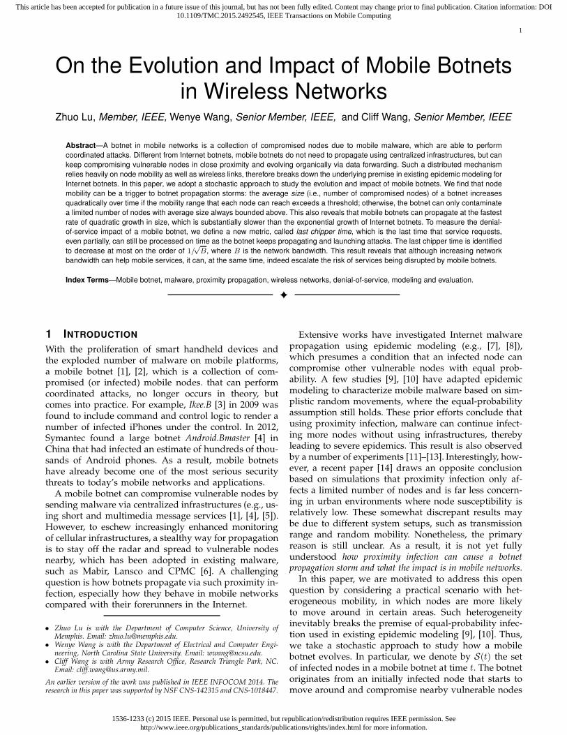
Fig. 2. Mobile botnet evolution over time via proximityinfection.

Accordingly, we focus on the scenario in which mal-ware intends to use proximity infection to form a botnet.We consider the malware infection process starting fromone initially infected node that attempts to propagatemalware to other vulnerable nodes in the network. Asshown in Fig. 2, a compromised node propagates mal-ware to the other node when (i) the two nodes mustmove into each other’s wireless transmission range r; (ii)the other node must be susceptible to malware (a vul-nerability ratio κ∈(0, 1) is used to denote the probabilitythat a node is vulnerable); and (iii) the required infectiontime (how long it takes to infect a node) is randomlydistributed in a range [δ1, δ2]. This is because the spreadof malware requires some time for user or applicationinteraction. If two nodes move out of each other’s rangeand have no time to finish the interaction, a node cannotbe infected even if it is vulnerable. Thus, our model alsoaccommodates the case of limited contact or interactiontime.

2.2.1 Node Mobility

Mobility plays an essential role in the performanceof mobile applications, and accordingly has substantialimpacts on malware propagation [13]. We consider ageneric mobility model that accounts for a practicalscenario of spatial heterogeneity, in which mobile nodesare more likely to stay in certain areas (e.g., their homesor offices) and less likely to be in others. In particular,similar to existing works [15], [16], we define the follow-ing generic mobility mode.

Definition 1: For a mobile node mi, there exist a homepoint hmi

, which is independently and uniformly dis-tributed over region Ω. A mobility radius α for mi isdefined such that mi moves around hmi

with probabilitydensity function Ψ(x), which is invariant in all directionsand satisfies

Ψ(x) > 0 when ‖x − hmi‖ ≤ α,

Ψ(x) = 0 otherwise.

In addition, all mobile nodes move around their homepoints according to independent stationary processes.

It is worth mentioning that a home point in this paperis simply an anchor point for the mathematical model tospecify the mobile range of a user. It does not mean thatthe user will be around this point more frequently. Amobile node mi can frequently visit several places, suchas workplace, school, and mall, as long as they are inthe mobile range specified by the home point hmi

andthe radius α.

We assume that malware can only compromise thesoftware in a vulnerable node, but cannot decide thenode’s movement since mobility is usually determinedby human beings.

2.3 Problem Formulation

As the initially infected node moves around and intendsto spread malware to other vulnerable nodes startingfrom time 0, it can be expected that more and more nodesare infected and repeat the same infection process in thenetwork. Therefore, a large-scale mobile botnet might bebuilt from the scratch with sufficient time. Such a botnetcould be very detrimental to mobile users as well asmobile service operations.

In order to understand the potential impact of a mobilebotnet, we first need to investigate how it evolves overtime; i.e., we are interested in how many nodes in totalhave been infected at a particular time t. To proceed, wedefine the size of a mobile botnet as follows.

Definition 2: A mobile botnet, denoted by S(t), is theset of all malware-infected nodes at time t. The size ofthe botnet |S(t)| is defined as the total number of nodesin S(t).

With Definition 2, we further characterize how fasta mobile botnet can spread malware in the network.Specifically, we define the evolution speed of a botnetin the following.

Definition 3: The evolution speed of a mobile botnet,denoted by V (t), is defined as V (t) = E|S(t)|/t, whereE|S(t)| is the average number of nodes in S(t) at time t.

Given Definitions 2 and 3, we formally state ourresearch problem: for a mobile botnet originated fromone initially infected node at time 0, what its size |S(t)|and evolution speed V (t) are at time t > 0?

3 HOW DOES A MOBILE BOTNET EVOLVE

OVER TIME?

In this section, we first investigate the size of a mobilebotnet |S(t)| and its evolution speed V (t), then usemobility traces to show botnet propagation in realisticenvironments.

3.1 The Average Size and Evolution Speed

From Definition 3, we know that the evolution speed ofa botnet V (t) is based on the average size E|S(t)|. Thus,it is essential to investigate the size of a mobile botnetat time t. We first prove the following lemma that willbe used later.



4

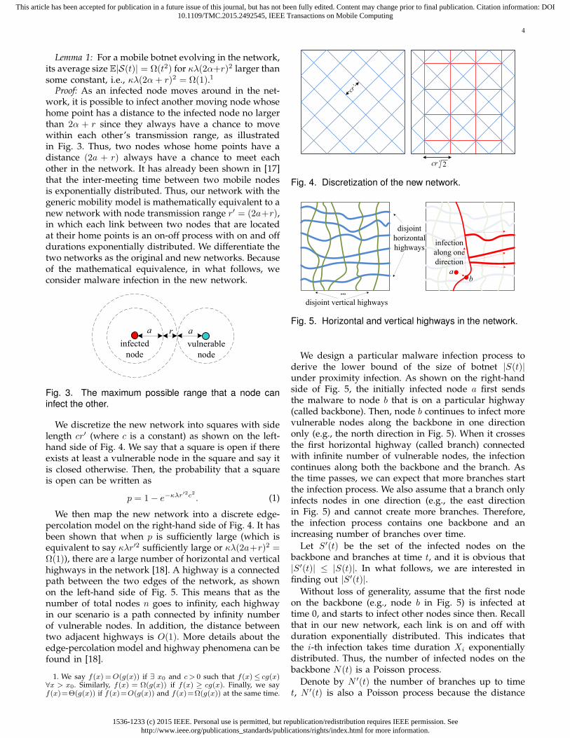
Lemma 1: For a mobile botnet evolving in the network,its average size E|S(t)| = Ω(t2) for κλ(2α+r)2 larger thansome constant, i.e., κλ(2α + r)2 = Ω(1).1

Proof: As an infected node moves around in the net-work, it is possible to infect another moving node whosehome point has a distance to the infected node no largerthan 2α + r since they always have a chance to movewithin each other’s transmission range, as illustratedin Fig. 3. Thus, two nodes whose home points have adistance (2a + r) always have a chance to meet eachother in the network. It has already been shown in [17]that the inter-meeting time between two mobile nodesis exponentially distributed. Thus, our network with thegeneric mobility model is mathematically equivalent to anew network with node transmission range r′ = (2a+r),in which each link between two nodes that are locatedat their home points is an on-off process with on and offdurations exponentially distributed. We differentiate thetwo networks as the original and new networks. Becauseof the mathematical equivalence, in what follows, weconsider malware infection in the new network.

ra a

infected

node

vulnerable

node

Fig. 3. The maximum possible range that a node caninfect the other.

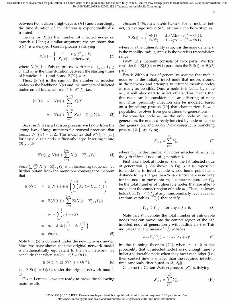
We discretize the new network into squares with sidelength cr′ (where c is a constant) as shown on the left-hand side of Fig. 4. We say that a square is open if thereexists at least a vulnerable node in the square and say itis closed otherwise. Then, the probability that a squareis open can be written as

p = 1 − e−κλr′2c2

. (1)

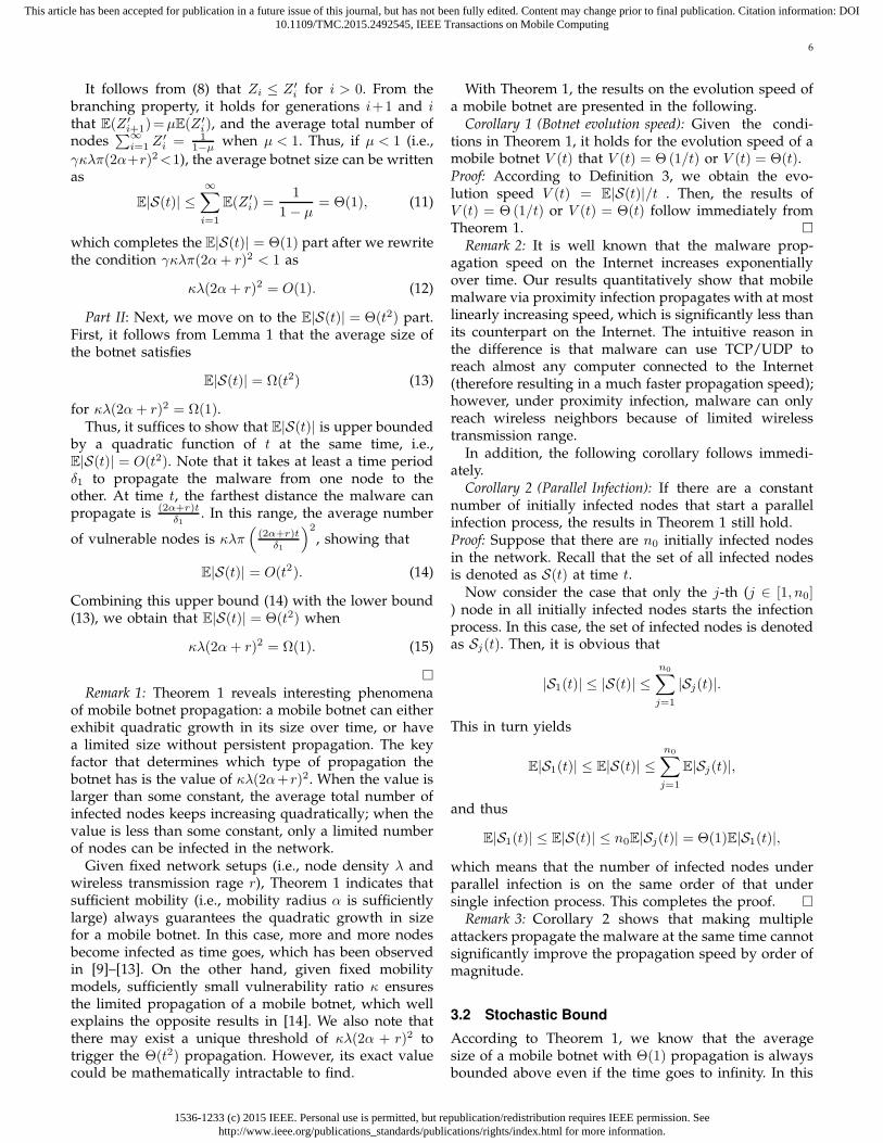
We then map the new network into a discrete edge-percolation model on the right-hand side of Fig. 4. It hasbeen shown that when p is sufficiently large (which isequivalent to say κλr′2 sufficiently large or κλ(2a+r)2 =Ω(1)), there are a large number of horizontal and verticalhighways in the network [18]. A highway is a connectedpath between the two edges of the network, as shownon the left-hand side of Fig. 5. This means that as thenumber of total nodes n goes to infinity, each highwayin our scenario is a path connected by infinity numberof vulnerable nodes. In addition, the distance betweentwo adjacent highways is O(1). More details about theedge-percolation model and highway phenomena can befound in [18].

1. We say f(x) = O(g(x)) if ∃ x0 and c > 0 such that f(x)≤ cg(x)∀x > x0. Similarly, f(x) = Ω(g(x)) if f(x) ≥ cg(x). Finally, we sayf(x)=Θ(g(x)) if f(x)=O(g(x)) and f(x)=Ω(g(x)) at the same time.

2cr’

Fig. 4. Discretization of the new network.

disjoint

horizontal

highways

disjoint vertical highways

...

infection

along one

direction

a

b

Fig. 5. Horizontal and vertical highways in the network.

We design a particular malware infection process toderive the lower bound of the size of botnet |S(t)|under proximity infection. As shown on the right-handside of Fig. 5, the initially infected node a first sendsthe malware to node b that is on a particular highway(called backbone). Then, node b continues to infect morevulnerable nodes along the backbone in one directiononly (e.g., the north direction in Fig. 5). When it crossesthe first horizontal highway (called branch) connectedwith infinite number of vulnerable nodes, the infectioncontinues along both the backbone and the branch. Asthe time passes, we can expect that more branches startthe infection process. We also assume that a branch onlyinfects nodes in one direction (e.g., the east directionin Fig. 5) and cannot create more branches. Therefore,the infection process contains one backbone and anincreasing number of branches over time.

Let S′(t) be the set of the infected nodes on thebackbone and branches at time t, and it is obvious that|S′(t)| ≤ |S(t)|. In what follows, we are interested infinding out |S′(t)|.

Without loss of generality, assume that the first nodeon the backbone (e.g., node b in Fig. 5) is infected attime 0, and starts to infect other nodes since then. Recallthat in our new network, each link is on and off withduration exponentially distributed. This indicates thatthe i-th infection takes time duration Xi exponentiallydistributed. Thus, the number of infected nodes on thebackbone N(t) is a Poisson process.

Denote by N ′(t) the number of branches up to timet, N ′(t) is also a Poisson process because the distance



5

between two adjacent highways is O(1) and accordinglythe time duration of an infection is exponentially dis-tributed.

Denote by X ′i(t) the number of infected nodes on

branch i. Using a similar argument, we can show thatX ′

i(t) is a delayed Poisson process satisfying

X ′i(t) =

0 t ≤∑ij=1 Yj

Xi(τ) otherwise,(2)

where Xi(τ) is a Poisson process with τ = t−∑ij=1 Yj ≥

0, and Yj is the time duration between the starting timesof branches i − 1 and i, and E(Yj) = ∆.

Thus, |S′(t)| is the sum of the number of infectednodes on the backbone N(t) and the numbers of infectednodes on all branches from 1 to N ′(t); i.e.,

|S′(t)| = N(t) +

N ′(t)∑

i=1

X ′i(t)

= N(t) +

N ′(t)∑

i=1

Xi(t − Σij=1Yj). (3)

Because N ′(t) is a Poisson process, we know from thestrong law of large numbers for renewal processes thatlimt→∞ N ′(t)/t = 1/∆. This indicates that N ′(t) ≥ ⌊βt⌋for any β < 1/∆ and t sufficiently large. Inserting it into(3) yields

|S′(t)| ≥ N(t) +

⌊βt⌋∑

i=1

Xi(t − Σij=1Yj). (4)

Since∑⌊βt⌋

i=1 Xi(t−Σij=1Yj) is an increasing sequence, we

further obtain from the monotone convergence theoremthat

E|S′(t)| ≥ E(N(t)) + E

⌊βt⌋∑

i=1

Xi(t − Σij=1Yj)

= E(N(t)) +

⌊βt⌋∑

i=1

E(Xi(t − Σij=1Yj))

= σt +

⌊βt⌋∑

i=1

δ(t − i∆)

= σt + δ⌊βt⌋(

t − ∆⌊βt⌋

2

)

= Θ(t2). (5)

Note that (5) is obtained under the new network model.Since we have shown that the original network modelis mathematically equivalent to the new network, weconclude that when κλ(2a + r)2 = Ω(1),

E|S(t)| ≥ E(|S′(t)|) ≥ Θ(t2); (6)

i.e., E|S(t)| = Ω(t2), under the original network model.

Given Lemma 1, we are ready to prove the followingmain results.

Theorem 1 (Size of a mobile botnet): For a mobile bot-net, its average size E|S(t)| at time t can be written as

E|S(t)| =

Θ(1) if κλ(2α + r)2 = O(1),Θ(t2) if κλ(2α + r)2 = Ω(1),

where κ is the vulnerability ratio, λ is the node density, αis the mobility radius, and r is the wireless transmissionrange.

Proof: This theorem consists of two parts. We firstconsider the E|S(t)| = Θ(1) part, then the E|S(t)| = Θ(t2)part.

Part I: Without loss of generality, assume that mobilenode m1 is the initially infect node that moves aroundin the network and attempts to infect vulnerable nodesas many as possible. Once a node is infected by nodem1, it will also start to infect others. This means thatthis node can be considered as an offspring of nodem1. Thus, proximity infection can be modeled basedon a branching process [19] that characterizes how apopulation evolves from generations to generations.

We consider node m1 as the only node in the 1stgeneration, the nodes directly infected by node m1 as the2nd generation, and so on. Now construct a branchingprocess Zi satisfying

Zi+1 =

Zi∑

j=1

Yi,j , (7)

where Yi,j is the number of nodes infected directly bythe j-th infected node of generation i.

First take a look at node m1 (i.e., the 1st infected nodeof generation 1). As shown in Fig. 3, it is impossiblefor node m1 to infect a node whose home point has adistance to m1’s larger than 2α+ r since there is no wayfor the node to move into m1’s contact region. Let Y ′

1,1

be the total number of vulnerable nodes that are able tomove into the contact region of node m1. Then, it alwaysholds that Y1,1 ≤ Y ′

1,1 at any time. Similarly, we have i.i.d.random variables Y ′

i,j that satisfy

Yi,j ≤ Y ′i,j for any i, j > 0. (8)

Note that Y ′i,j denotes the total number of vulnerable

nodes that can move into the contact region of the i-thinfected node of generation j with radius 2α + r. Thisindicates that the mean of Y ′

i,j satisfies

µ = E(Y ′i,j) = γκλπ(2α + r)2 (9)

by the thinning theorem [20], where γ > 0 is theprobability that an infected node has no enough time toinfect a vulnerable node when they meet each other (i.e.,their contact time is smaller than the required infectiontime randomly distributed in [δ1, δ2]).

Construct a Galton-Watson process Z ′i satisfying

Z ′i+1 =

Z′

i∑

j=1

Y ′i,j . (10)



6

It follows from (8) that Zi ≤ Z ′i for i > 0. From the

branching property, it holds for generations i+1 and ithat E(Z ′

i+1)=µE(Z ′i), and the average total number of

nodes∑∞

i=1 Z ′i = 1

1−µwhen µ < 1. Thus, if µ < 1 (i.e.,

γκλπ(2α+r)2 <1), the average botnet size can be writtenas

E|S(t)| ≤∞∑

i=1

E(Z ′i) =

1

1 − µ= Θ(1), (11)

which completes the E|S(t)| = Θ(1) part after we rewritethe condition γκλπ(2α + r)2 < 1 as

κλ(2α + r)2 = O(1). (12)

Part II: Next, we move on to the E|S(t)| = Θ(t2) part.First, it follows from Lemma 1 that the average size ofthe botnet satisfies

E|S(t)| = Ω(t2) (13)

for κλ(2α + r)2 = Ω(1).Thus, it suffices to show that E|S(t)| is upper bounded

by a quadratic function of t at the same time, i.e.,E|S(t)| = O(t2). Note that it takes at least a time periodδ1 to propagate the malware from one node to theother. At time t, the farthest distance the malware canpropagate is (2α+r)t

δ1

. In this range, the average number

of vulnerable nodes is κλπ(

(2α+r)tδ1

)2

, showing that

E|S(t)| = O(t2). (14)

Combining this upper bound (14) with the lower bound(13), we obtain that E|S(t)| = Θ(t2) when

κλ(2α + r)2 = Ω(1). (15)

Remark 1: Theorem 1 reveals interesting phenomenaof mobile botnet propagation: a mobile botnet can eitherexhibit quadratic growth in its size over time, or havea limited size without persistent propagation. The keyfactor that determines which type of propagation thebotnet has is the value of κλ(2α+ r)2. When the value islarger than some constant, the average total number ofinfected nodes keeps increasing quadratically; when thevalue is less than some constant, only a limited numberof nodes can be infected in the network.

Given fixed network setups (i.e., node density λ andwireless transmission rage r), Theorem 1 indicates thatsufficient mobility (i.e., mobility radius α is sufficientlylarge) always guarantees the quadratic growth in sizefor a mobile botnet. In this case, more and more nodesbecome infected as time goes, which has been observedin [9]–[13]. On the other hand, given fixed mobilitymodels, sufficiently small vulnerability ratio κ ensuresthe limited propagation of a mobile botnet, which wellexplains the opposite results in [14]. We also note thatthere may exist a unique threshold of κλ(2α + r)2 totrigger the Θ(t2) propagation. However, its exact valuecould be mathematically intractable to find.

With Theorem 1, the results on the evolution speed ofa mobile botnet are presented in the following.

Corollary 1 (Botnet evolution speed): Given the condi-tions in Theorem 1, it holds for the evolution speed of amobile botnet V (t) that V (t) = Θ (1/t) or V (t) = Θ(t).Proof: According to Definition 3, we obtain the evo-lution speed V (t) = E|S(t)|/t . Then, the results ofV (t) = Θ (1/t) or V (t) = Θ(t) follow immediately fromTheorem 1.

Remark 2: It is well known that the malware prop-agation speed on the Internet increases exponentiallyover time. Our results quantitatively show that mobilemalware via proximity infection propagates with at mostlinearly increasing speed, which is significantly less thanits counterpart on the Internet. The intuitive reason inthe difference is that malware can use TCP/UDP toreach almost any computer connected to the Internet(therefore resulting in a much faster propagation speed);however, under proximity infection, malware can onlyreach wireless neighbors because of limited wirelesstransmission range.

In addition, the following corollary follows immedi-ately.

Corollary 2 (Parallel Infection): If there are a constantnumber of initially infected nodes that start a parallelinfection process, the results in Theorem 1 still hold.Proof: Suppose that there are n0 initially infected nodesin the network. Recall that the set of all infected nodesis denoted as S(t) at time t.

Now consider the case that only the j-th (j ∈ [1, n0]) node in all initially infected nodes starts the infectionprocess. In this case, the set of infected nodes is denotedas Sj(t). Then, it is obvious that

|S1(t)| ≤ |S(t)| ≤n0∑

j=1

|Sj(t)|.

This in turn yields

E|S1(t)| ≤ E|S(t)| ≤n0∑

j=1

E|Sj(t)|,

and thus

E|S1(t)| ≤ E|S(t)| ≤ n0E|Sj(t)| = Θ(1)E|S1(t)|,

which means that the number of infected nodes underparallel infection is on the same order of that undersingle infection process. This completes the proof.

Remark 3: Corollary 2 shows that making multipleattackers propagate the malware at the same time cannotsignificantly improve the propagation speed by order ofmagnitude.

3.2 Stochastic Bound

According to Theorem 1, we know that the averagesize of a mobile botnet with Θ(1) propagation is alwaysbounded above even if the time goes to infinity. In this



7

case, we are also interested in what the distribution ofits eventual size is, which is given in the following.

Theorem 2: The tail distribution of the eventual size ofa botnet P(|S(∞)| > L) decays at least exponentially fastwhen κλ(2α + r)2 = O(1).

Proof: Recall that we have already constructed a pro-cess in (10) that satisfies

P(|S(∞)| > L) ≤ P

(

∞∑

i=1

Z ′i > L

)

. (16)

Then, it suffices to show that the distribution of∑∞

i=1 Z ′i

decays exponentially fast.First, according to the total progeny theorem (Propo-

sition 3.4 in [19]), we obtain

P

(

∞∑

i=1

Z ′i = l

)

=P

(

∑li=1 Y ′

l,i = l − 1)

l, (17)

where Y ′l,i is the number of vulnerable nodes whose

home points fall into a circle with radius 2α + r. Withthe network size scaling, node distribution can be rep-resented as a Poisson point process [21], [22]. Thus, itholds for Y ′

l,i that

P

(

l∑

i=1

Y ′l,i = l − 1

)

=(lµ)l−1e−lµ

(l − 1)!, (18)

where µ is given in (9). Inserting (18) into (17) yields

P

(

∞∑

i=1

Z ′i = l

)

=(lµ)l−1e−lµ

l!. (19)

Applying Stirling’s formula

l! = Θ(1)ll+1

2 e−l

to (19), we obtain

P

(

∞∑

i=1

Z ′i = l

)

= Θ(1)l−3

2 µl−1e−l(µ−1). (20)

Therefore, it follows from (20) that

liml→∞

log P(∑∞

i=1Z′i = l)

l

= liml→∞

Θ(1) − 32 log l + (l − 1) log µ − (µ − 1)

l

= log µ − liml→∞

1.5 log l

l= Θ(1), (21)

showing that P(∑∞

i=1 Z ′i) decays exponentially, which

completes the proof.

Remark 4: Theorem 2 shows that if κλ(2α + r)2 issufficiently small, the distribution of the size of a mobilebotnet exhibits at least exponential decay; i.e., its taildistribution is bounded from above by an exponentialdistribution. In this case, it is quite unlikely that a botnetcan infect a large number of nodes in the network andcause severe impacts on mobile services.

3.3 Experimental Evaluation

In addition to theoretical analysis, we use experimentsbased on mobility traces to investigate mobile botnetpropagation in realistic environments. In our experi-ments, we generate mobile nodes on a fixed-size map.Each node moves around according to realistic mobilitytraces. We randomly choose one node as the initiallyinfected node that attempts to propagate malware toother vulnerable nodes. If a node moves into the wirelesstransmission range of an infected node and at the sametime it is vulnerable, it will become an infected node thatstarts to infect others.

0 4 8 12

50

100

150

200

Days

Siz

e o

f B

otn

et

WiFi

Bluetooth

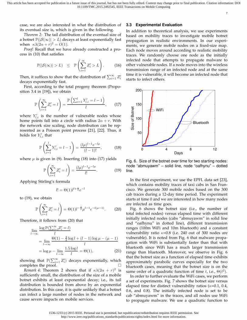
Fig. 6. Size of the botnet over time for two starting nodes:node “abmuyawm” – solid line, node “oafhynu” – dotted

line.

In the first experiment, we use the EPFL data set [23],which contains mobility traces of taxi cabs in San Fran-cisco. We generate 300 mobile nodes based on the 300cab traces during a 12-day time period. The experimentstarts at time 0 and we are interested in how many nodesare infected as time goes.

Fig. 6 shows the botnet size (i.e., the number oftotal infected nodes) versus elapsed time with differentinitially infected nodes (cabs “abmuyawm” in solid lineand “oafhynu” in dotted line), different transmissionranges (100m WiFi and 10m bluetooth) and a constantvulnerability ratio κ=0.8 (i.e. 240 out of 300 nodes arevulnerable). It is noted from Fig. 6 that malware propa-gation with WiFi is substantially faster than that withbluetooth since WiFi has a much larger transmissionrange than bluetooth. Moreover, we observe in Fig. 6that the botnet size as a function of elapsed time exhibitsapproximately parabolic curves especially for the twobluetooth cases, meaning that the botnet size is on thesame order of a quadratic function of time t, i.e., Θ(t2).

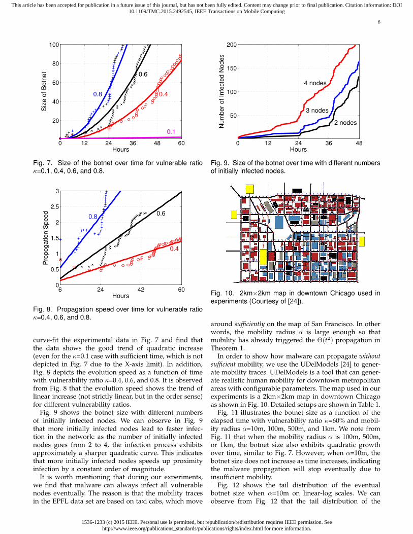
In order to further evaluate the WiFi cases, we performa set of experiments. Fig. 7 shows the botnet size versuselapsed time for distinct vulnerability ratios (κ=0.1, 0.4,0.6, and 0.8). The initially infected node is set to becab “abmuyawm” in the traces, and all nodes use WiFito propagate malware. We use a quadratic function to



8

0 12 24 36 48 60

20

40

60

80

100

Hours

Siz

e o

f B

otn

et

0.4

0.6

0.8

0.1

Fig. 7. Size of the botnet over time for vulnerable ratioκ=0.1, 0.4, 0.6, and 0.8.

6 24 42 600

0.5

1

1.5

2

2.5

3

Hours

Pro

pogation S

peed

0.4

0.60.8

Fig. 8. Propagation speed over time for vulnerable ratioκ=0.4, 0.6, and 0.8.

curve-fit the experimental data in Fig. 7 and find thatthe data shows the good trend of quadratic increase(even for the κ=0.1 case with sufficient time, which is notdepicted in Fig. 7 due to the X-axis limit). In addition,Fig. 8 depicts the evolution speed as a function of timewith vulnerability ratio κ=0.4, 0.6, and 0.8. It is observedfrom Fig. 8 that the evolution speed shows the trend oflinear increase (not strictly linear, but in the order sense)for different vulnerability ratios.

Fig. 9 shows the botnet size with different numbersof initially infected nodes. We can observe in Fig. 9that more initially infected nodes lead to faster infec-tion in the network: as the number of initially infectednodes goes from 2 to 4, the infection process exhibitsapproximately a sharper quadratic curve. This indicatesthat more initially infected nodes speeds up proximityinfection by a constant order of magnitude.

It is worth mentioning that during our experiments,we find that malware can always infect all vulnerablenodes eventually. The reason is that the mobility tracesin the EPFL data set are based on taxi cabs, which move

0 12 24 36 48

50

100

150

200

Hours

Num

ber

of In

fecte

d N

odes

2 nodes

3 nodes

4 nodes

Fig. 9. Size of the botnet over time with different numbersof initially infected nodes.

Fig. 10. 2km×2km map in downtown Chicago used in

experiments (Courtesy of [24]).

around sufficiently on the map of San Francisco. In otherwords, the mobility radius α is large enough so thatmobility has already triggered the Θ(t2) propagation inTheorem 1.

In order to show how malware can propagate withoutsufficient mobility, we use the UDelModels [24] to gener-ate mobility traces. UDelModels is a tool that can gener-ate realistic human mobility for downtown metropolitanareas with configurable parameters. The map used in ourexperiments is a 2km×2km map in downtown Chicagoas shown in Fig. 10. Detailed setups are shown in Table 1.

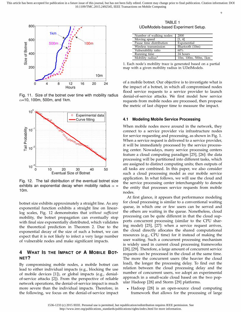
Fig. 11 illustrates the botnet size as a function of theelapsed time with vulnerability ratio κ=60% and mobil-ity radius α=10m, 100m, 500m, and 1km. We note fromFig. 11 that when the mobility radius α is 100m, 500m,or 1km, the botnet size also exhibits quadratic growthover time, similar to Fig. 7. However, when α=10m, thebotnet size does not increase as time increases, indicatingthe malware propagation will stop eventually due toinsufficient mobility.

Fig. 12 shows the tail distribution of the eventualbotnet size when α=10m on linear-log scales. We canobserve from Fig. 12 that the tail distribution of the



9

0 4 8 12 16 20 24

200

400

600

800

Hours

Siz

e o

f B

otn

et

10m

1km

100m500m

Fig. 11. Size of the botnet over time with mobility radiusα=10, 100m, 500m, and 1km.

0 10 20 30 40 5010

−3

10−2

10−1

100

Eventual Size of Botnet

Tail

Pro

babili

ty

Experimental data

Curve fitting

Fig. 12. The tail distribution of the eventual botnet size

exhibits an exponential decay when mobility radius α =10m.

botnet size exhibits approximately a straight line. As anyexponential function exhibits a straight line on linear-log scales, Fig. 12 demonstrates that without sufficientmobility, the botnet propagation can eventually stopwith final size exponentially distributed, which validatesthe theoretical prediction in Theorem 2. Due to theexponential decay of the size of such a botnet, we canexpect that it is not likely to infect a very large numberof vulnerable nodes and make significant impacts.

4 WHAT IS THE IMPACT OF A MOBILE BOT-NET?

By compromising mobile nodes, a mobile botnet canlead to either individual impacts (e.g., blocking the useof mobile devices [1]), or global impacts (e.g., denial-of-service attacks [2]). From the perspective of reliablenetwork operations, the denial-of-service impact is muchmore severe than the individual impacts. Therefore, inthe following, we focus on the denial-of-service impact

TABLE 1UDelModels-based Experiment Setup.

Number of walking nodes: 2000Moving speed [1, 4]Pause time distribution ExponentialWireless transmission Bluetooth (10m)Vulnerability ratio 60%Running time 24 hoursMobility radius1 10m, 100m, 500m, 1km

1. Each node’s mobility trace is generated based on a partialmap with a given mobility radius in UDelModels.

of a mobile botnet. Our objective is to investigate what isthe impact of a botnet, in which all compromised nodesflood service requests to a service provider to launchdenial-of-service attacks. We first model how servicerequests from mobile nodes are processed, then proposethe metric of last chipper time to measure the impact.

4.1 Modeling Mobile Service Processing

When mobile nodes move around in the network, theyconnect to a service provider via infrastructure nodesfor service requesting and processing, as shown in Fig. 1.When a service request is delivered to a service provider,it will be immediately processed by the service process-ing center. Nowadays, many service processing centersfeature a cloud computing paradigm [25], [26]: the dataprocessing will be partitioned into different tasks, whichare assigned to distinct computing units; then outputs ofall tasks are combined. In this paper, we also considersuch a cloud processing model as our mobile serviceapplication. In what follows, we will use the cloud andthe service processing center interchangeably to denotethe entity that processes service requests from mobilenodes.

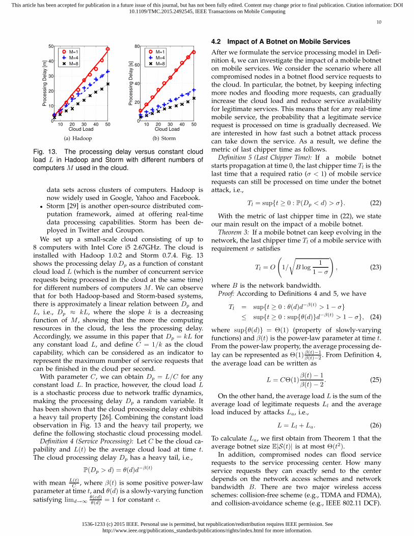
At first glance, it appears that performance modelingfor cloud processing is similar to a conventional waitingqueue, in which one or few users can be served andthe others are waiting in the queue. Nonetheless, cloudprocessing can be quite different in that the cloud sup-ports concurrent processing (similar to the CPU shar-ing model) [25], [27]: when a service request arrives,the cloud directly allocates the shared computationalresources (e.g., CPU time) for it instead of making theuser waiting. Such a concurrent processing mechanismis widely used in current cloud processing frameworks[28], [29]. Therefore, a large amount of concurrent servicerequests can be processed in the cloud at the same time.The more the concurrent users (the heavier the cloudload), the longer the processing delay. To find out therelation between the cloud processing delay and thenumber of concurrent users, we adopt an experimentalapproach in a small-scale cloud based on the two pop-ular Hadoop [28] and Storm [29] platforms.

• Hadoop [28] is an open-source cloud computingframework that allows for the processing of large



10

10 20 30 40 500

10

20

30

40

50

Cloud Load

Pro

cessin

g D

ela

y [m

]

M=1

M=4

M=8

(a) Hadoop

10 20 30 40 500

20

40

60

80

Cloud LoadP

rocessin

g D

ela

y [s]

M=1

M=4

M=8

(b) Storm

Fig. 13. The processing delay versus constant cloud

load L in Hadoop and Storm with different numbers ofcomputers M used in the cloud.

data sets across clusters of computers. Hadoop isnow widely used in Google, Yahoo and Facebook.

• Storm [29] is another open-source distributed com-putation framework, aimed at offering real-timedata processing capabilities. Storm has been de-ployed in Twitter and Groupon.

We set up a small-scale cloud consisting of up to8 computers with Intel Core i5 2.67GHz. The cloud isinstalled with Hadoop 1.0.2 and Storm 0.7.4. Fig. 13shows the processing delay Dp as a function of constantcloud load L (which is the number of concurrent servicerequests being processed in the cloud at the same time)for different numbers of computers M . We can observethat for both Hadoop-based and Storm-based systems,there is approximately a linear relation between Dp andL, i.e., Dp ≈ kL, where the slope k is a decreasingfunction of M , showing that the more the computingresources in the cloud, the less the processing delay.Accordingly, we assume in this paper that Dp = kL forany constant load L, and define C = 1/k as the cloudcapability, which can be considered as an indicator torepresent the maximum number of service requests thatcan be finished in the cloud per second.

With parameter C, we can obtain Dp = L/C for anyconstant load L. In practice, however, the cloud load Lis a stochastic process due to network traffic dynamics,making the processing delay Dp a random variable. Ithas been shown that the cloud processing delay exhibitsa heavy tail property [26]. Combining the constant loadobservation in Fig. 13 and the heavy tail property, wedefine the following stochastic cloud processing model.

Definition 4 (Service Processing): Let C be the cloud ca-pability and L(t) be the average cloud load at time t.The cloud processing delay Dp has a heavy tail, i.e.,

P(Dp > d) = θ(d)d−β(t)

with mean L(t)C

, where β(t) is some positive power-lawparameter at time t, and θ(d) is a slowly-varying function

satisfying limd→∞θ(cd)θ(d) = 1 for constant c.

4.2 Impact of A Botnet on Mobile Services

After we formulate the service processing model in Defi-nition 4, we can investigate the impact of a mobile botneton mobile services. We consider the scenario where allcompromised nodes in a botnet flood service requests tothe cloud. In particular, the botnet, by keeping infectingmore nodes and flooding more requests, can graduallyincrease the cloud load and reduce service availabilityfor legitimate services. This means that for any real-timemobile service, the probability that a legitimate servicerequest is processed on time is gradually decreased. Weare interested in how fast such a botnet attack processcan take down the service. As a result, we define themetric of last chipper time as follows.

Definition 5 (Last Chipper Time): If a mobile botnetstarts propagation at time 0, the last chipper time Tl is thelast time that a required ratio (σ < 1) of mobile servicerequests can still be processed on time under the botnetattack, i.e.,

Tl = supt ≥ 0 : P(Dp < d) > σ. (22)

With the metric of last chipper time in (22), we stateour main result on the impact of a mobile botnet.

Theorem 3: If a mobile botnet can keep evolving in thenetwork, the last chipper time Tl of a mobile service withrequirement σ satisfies

Tl = O

(

1/

√

B log1

1 − σ

)

, (23)

where B is the network bandwidth.Proof: According to Definitions 4 and 5, we have

Tl = supt ≥ 0 : θ(d)d−β(t) > 1 − σ≤ supt ≥ 0 : supθ(d)d−β(t) > 1 − σ, (24)

where supθ(d) = Θ(1) (property of slowly-varyingfunctions) and β(t) is the power-law parameter at time t.From the power-law property, the average processing de-

lay can be represented as Θ(1)β(t)−1β(t)−2 . From Definition 4,

the average load can be written as

L = CΘ(1)β(t) − 1

β(t) − 2. (25)

On the other hand, the average load L is the sum of theaverage load of legitimate requests Ll and the averageload induced by attacks La, i.e.,

L = Ll + La. (26)

To calculate La, we first obtain from Theorem 1 that theaverage botnet size E|S(t)| is at most Θ(t2).

In addition, compromised nodes can flood servicerequests to the service processing center. How manyservice requests they can exactly send to the centerdepends on the network access schemes and networkbandwidth B. There are two major wireless accessschemes: collision-free scheme (e.g., TDMA and FDMA),and collision-avoidance scheme (e.g., IEEE 802.11 DCF).



11

In the former, network bandwidth B is partitioned intoorthogonal channels, each of which is used by only onenode. In the latter, B is shared among all nodes, whichuse a random backoff algorithm (e.g., binary exponen-tial backoff) to access the wireless channel. No matterwhat access scheme the network has, the maximumbandwidth available for a node is always no greaterthan network bandwidth B, which indicates the rate offlooded requests at each compromised node is alwaysupper bounded by O(B).

Therefore, the average load induced by attacks La atthe service processing center is at most

La = CE(|S(t)|O(B)) = Ct2O(B). (27)

Then, It follows from (25), (26), and (27) that

β(t) = 2 +1

t2O(B). (28)

Inserting (28) into (24) completes the proof.

Theorem 3 shows that if a botnet can keep evolvingin the network, the last chipper time decreases at moston the order of 1/

√B. It has already been predicted

in existing work [1] that the risk of mobile malwareattack increases with the improved bandwidth in futurewireless networks. Theorem 3 gives an interesting as-sessment on how such a risk is boosted. For example,LTE advanced is planned to improve the LTE uplinkspeed 10 times (from 50 Mbps to 500 Mbps). It followsfrom Theorem 3 that for the same mobile service, its lastchipper time in LTE advanced will become around onethird of the time in LTE (1/

√10 ≈ 1/3). This means that

in order to make some impact in LTE advanced, a botnetonly needs to propagate one third of the time that itspends in LTE.

Remark 5: It is worthy of note that the decrease onthe order of 1/

√B of the last chipper time relies on the

condition that all infected nodes attempt to saturate thenetwork channel to launch attacks. If they attack at aconstant rate that does not depend on B, the last chippertime should not be affected by B. Therefore, practicalnetworks must always deploy attack detection and rate-limiting schemes to prevent infected nodes from floodingservice requests at the saturated rate. However, we dobelieve that the decrease on the order of 1/

√B represents

the worst-case scenario that should be considered for anyrisk assessment of mobile botnets.

4.3 Experimental Evaluation

We also use experiments to measure the last chippertime. We first present the setups, then discuss the results.

4.3.1 System Setups

We set up a small-scale cloud that consists of 8 comput-ers running over the Storm framework [29]. As shownin Fig. 14, the cloud is connected to a simulation serverthat simulates a wireless network environment.

...

...

...

the cloud the network

service

processed

simulation server

requests

results...

Fig. 14. A small-scale cloud is connected to a networksimulation server.

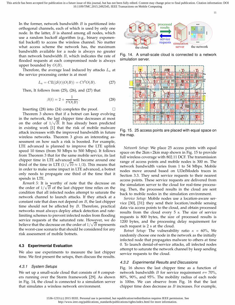
Fig. 15. 25 access points are placed with equal space onthe map.

Network Setup: We place 25 access points with equalspace on the 2km×2km map shown in Fig. 15 to providefull wireless coverage with 802.11 DCF. The transmissionrange of access points and mobile nodes is 300 m. Thenetwork bandwidth varies from 1 to 54 Mbps. Mobilenodes move around based on UDelModels traces inSection 3.3. They send service requests to their nearestaccess points. These service requests are delivered fromthe simulation server to the cloud for real-time process-ing. Then, the processed results in the cloud are sentback to mobile nodes in the simulation environment.

Service Setup: Mobile nodes use a location-aware ser-vice [30], [31]: they send their location/mobile sensingdata via access points to the cloud, and obtain processedresults from the cloud every 5 s. The size of servicerequests is 800 bytes, the size of processed results is1200 bytes, and the processing delay requirement foreach request is 2 s at the cloud.

Botnet Setup: The vulnerability ratio κ = 60%, Werandomly choose one node in the network as the initiallyinfected node that propagates malware to others at time0. To launch denial-of-service attacks, all infected nodesattempt to saturate the network channel by keep sendingservice requests to the cloud.

4.3.2 Experimental Results and Discussions

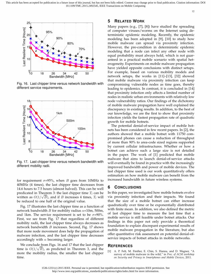
Fig. 16 shows the last chipper time as a function ofnetwork bandwidth B for service requirement σ= 70%,80%, 90%, and 95%. The mobility radius of each nodeis 100m. We can observe from Fig. 16 that the lastchipper time does decrease as B increases. For example,



12

10 18 26 34 42 505

10

15

20

25

Bandwidth [MHz]

Last R

esili

ent T

ime [H

ours

]

70%

90%

80%

95%

Fig. 16. Last chipper time versus network bandwidth withdifferent service requirements.

10 18 26 34 42 506

8

10

12

14

16

18

Bandwidth [MHz]

Last R

esili

ent T

ime [H

ours

]

1km

500m

100m

Fig. 17. Last chipper time versus network bandwidth withdifferent mobility radii.

for requirement σ=95%, when B goes from 10MHz to40MHz (4 times), the last chipper time decreases from14.6 hours to 7.5 hours (almost halved). This can be wellpredicated in Theorem 3: the last chipper time Tl can bewritten as O(1/

√B), and if B increases 4 times, Tl will

be reduced to one half of the original value.

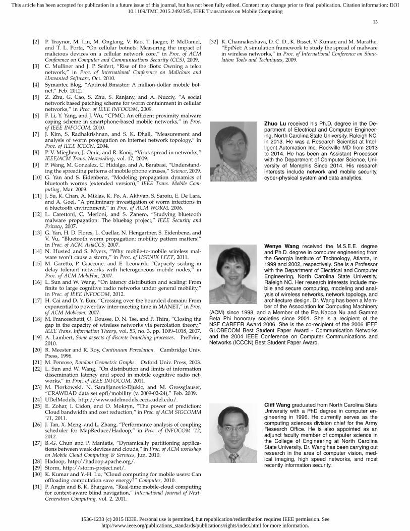
Fig. 17 illustrates the last chipper time as a function ofnetwork bandwidth B for mobility radius α=10m, 500m,and 1km. The service requirement is set to be σ=90%.First, we see from Fig. 17 that regardless of differentmobility radii, the last chipper time always decreases asnetwork bandwidth B increases. Second, Fig. 17 showsthat more node movement does help the propagation ofmalware infection, and the last chipper time decreasesaccordingly with α becoming larger.

We conclude from Figs. 16 and 17 that the last chippertime is O(1/

√B), as predicted in Theorem 3, and the

more the mobility radius, the smaller the last chippertime.

5 RELATED WORK

Many papers (e.g., [7], [8]) have studied the spreadingof computer viruses/worms on the Internet using de-terministic epidemic modeling. Recently, the epidemicmodeling has been adopted in [9], [10] to study howmobile malware can spread via proximity infection.However, the pre-condition in deterministic epidemicmodeling that a node can infect any other node withequal probability must always hold, which is not guar-anteed in a practical mobile scenario with spatial het-erogeneity. Experiments on mobile malware propagationhave yielded opposite conclusions with distinct setups.For example, based on various mobility models andnetwork setups, the works in [11]–[13], [32] showedthat mobile malware via proximity infection can keepcompromising vulnerable nodes as time goes, therebyleading to epidemics. In contrast, it is concluded in [14]that proximity infection only affects a limited number ofnodes in realistic urban environments with relatively lownode vulnerability ratios. Our findings of the dichotomyof mobile malware propagation have well explained thediscrepancy in existing results. In addition, to the best ofour knowledge, we are the first to show that proximityinfection yields the fastest propagation rate of quadraticgrowth for mobile botnets.

The potential denial-of-service impact of mobile bot-nets has been considered in few recent papers. In [2], theauthors showed that a mobile botnet with 11750 com-promised phones can cause a reduction of throughputof more than 90% to area-code sized regions supportedby current cellular infrastructures. Whether or how abotnet can achieve such a large size is not detailedin the paper. The work of [1] predicted that mobilemalware that aims to launch denial-of-service attackswill eventually be found in practice with the increasinglyimproved bandwidth and power of mobile devices. Thelast chipper time used is our work quantitatively offersestimation on how mobile malware can benefit from theincreased bandwidth in future wireless systems.

6 CONCLUSIONS

In this paper, we investigated how mobile botnets evolvevia proximity infection and their impacts. We foundthat the size of a mobile botnet can either increasequadratically over time or be exponentially distributedwith finite mean. In addition, we also defined the metricof last chipper time to measure the last time that amobile service is still feasible under botnet attacks. Ourfindings in this paper not only provide a theoreticalfoundation to explain discrepant experimental results ofmobile malware propagation in the literature, but alsooffer quantitative risk assessment on potential denial-of-service impacts of botnet attacks in mobile networks.

REFERENCES

[1] A. P. Felt, M. Finifter, E. Chin, S. Hanna, and D. Wagner, “Asurvey of mobile malware in the wild,” in Proc. of ACM workshopon Security and Privacy in Smartphones and Mobile Devices, 2011.



13

[2] P. Traynor, M. Lin, M. Ongtang, V. Rao, T. Jaeger, P. McDaniel,and T. L. Porta, “On cellular botnets: Measuring the impact ofmalicious devices on a cellular network core,” in Proc. of ACMConference on Computer and Communications Security (CCS), 2009.

[3] C. Mulliner and J. P. Seifert, “Rise of the iBots: Owning a telconetwork,” in Proc. of International Conference on Malicious andUnwanted Software, Oct. 2010.

[4] Symantec Blog, “Android.Bmaster: A million-dollar mobile bot-net,” Feb. 2012.

[5] Z. Zhu, G. Cao, S. Zhu, S. Ranjany, and A. Nucciy, “A socialnetwork based patching scheme for worm containment in cellularnetworks,” in Proc. of IEEE INFOCOM, 2009.

[6] F. Li, Y. Yang, and J. Wu, “CPMC: An efficient proximity malwarecoping scheme in smartphone-based mobile networks,” in Proc.of IEEE INFOCOM, 2010.

[7] J. Kim, S. Radhakrishnan, and S. K. Dhall, “Measurement andanalysis of worm propagation on internet network topology,” inProc. of IEEE ICCCN, 2004.

[8] P. V. Mieghem, J. Omic, and R. Kooij, “Virus spread in networks,”IEEE/ACM Trans. Networking, vol. 17, 2009.

[9] P. Wang, M. Gonzalez, C. Hidalgo, and A. Barabasi, “Understand-ing the spreading patterns of mobile phone viruses,” Science, 2009.

[10] G. Yan and S. Eidenbenz, “Modeling propagation dynamics ofbluetooth worms (extended version),” IEEE Trans. Mobile Com-puting, Mar. 2009.

[11] J. Su, K. Chan, A. Miklas, K. Po, A. Akhvan, S. Saroiu, E. De Lara,and A. Goel, “A preliminary investigation of worm infections ina bluetooth environment,” in Proc. of ACM WORM, 2006.

[12] L. Carettoni, C. Merloni, and S. Zanero, “Studying bluetoothmalware propagation: The bluebag project,” IEEE Security andPrivacy, 2007.

[13] G. Yan, H. D. Flores, L. Cuellar, N. Hengartner, S. Eidenbenz, andV. Vu, “Bluetooth worm propagation: mobility pattern matters!”in Proc. of ACM AsiaCCS, 2007.

[14] N. Husted and S. Myers, “Why mobile-to-mobile wireless mal-ware won’t cause a storm,” in Proc. of USENIX LEET, 2011.

[15] M. Garetto, P. Giaccone, and E. Leonardi, “Capacity scaling indelay tolerant networks with heterogeneous mobile nodes,” inProc. of ACM MobiHoc, 2007.

[16] L. Sun and W. Wang, “On latency distribution and scaling: Fromfinite to large cognitive radio networks under general mobility,”in Proc. of IEEE INFOCOM, 2012.

[17] H. Cai and D. Y. Eun, “Crossing over the bounded domain: Fromexponential to power-law inter-meeting time in MANET,” in Proc.of ACM Mobicom, 2007.

[18] M. Franceschetti, O. Dousse, D. N. Tse, and P. Thira, “Closing thegap in the capacity of wireless networks via percolation theory,”IEEE Trans. Information Theory, vol. 53, no. 3, pp. 1009–1018, 2007.

[19] A. Lambert, Some aspects of discrete branching processes. PrePrint,2010.

[20] R. Meester and R. Roy, Continuum Percolation. Cambridge Univ.Press, 1996.

[21] M. Penrose, Random Geometric Graphs. Oxford Univ. Press, 2003.[22] L. Sun and W. Wang, “On distribution and limits of information

dissemination latency and speed in mobile cognitive radio net-works,” in Proc. of IEEE INFOCOM, 2011.

[23] M. Piorkowski, N. Sarafijanovic-Djukic, and M. Grossglauser,“CRAWDAD data set epfl/mobility (v. 2009-02-24),” Feb. 2009.

[24] UDelModels, http://www.udelmodels.eecis.udel.edu/.[25] E. Zohar, I. Cidon, and O. Mokryn, “The power of prediction:

Cloud bandwidth and cost reduction,” in Proc. of ACM SIGCOMM’11, 2011.

[26] J. Tan, X. Meng, and L. Zhang, “Performance analysis of couplingscheduler for MapReduce/Hadoop,” in Proc. of INFOCOM ’12,2012.

[27] B.-G. Chun and P. Maniatis, “Dynamically partitioning applica-tions between weak devices and clouds,” in Proc. of ACM workshopon Mobile Cloud Computing & Services, Jun. 2010.

[28] Hadoop, http://hadoop.apache.org/.[29] Storm, http://storm-project.net/.[30] K. Kumar and Y.-H. Lu, “Cloud computing for mobile users: Can

offloading computation save energy?” Computer, 2010.[31] P. Angin and B. K. Bhargava, “Real-time mobile-cloud computing

for context-aware blind navigation,” International Journal of Next-Generation Computing, vol. 2, 2011.

[32] K. Channakeshava, D. C. D., K. Bisset, V. Kumar, and M. Marathe,“EpiNet: A simulation framework to study the spread of malwarein wireless networks,” in Proc. of International Conference on Simu-lation Tools and Techniques, 2009.

Zhuo Lu received his Ph.D. degree in the De-partment of Electrical and Computer Engineer-ing, North Carolina State University, Raleigh NC,in 2013. He was a Research Scientist at Intel-ligent Automation Inc, Rockville MD from 2013to 2014. He has been an Assistant Processorwith the Department of Computer Science, Uni-versity of Memphis Since 2014. His researchinterests include network and mobile security,cyber-physical system and data analytics.

Wenye Wang received the M.S.E.E. degreeand Ph.D. degree in computer engineering fromthe Georgia Institute of Technology, Atlanta, in1999 and 2002, respectively. She is a Professorwith the Department of Electrical and ComputerEngineering, North Carolina State University,Raleigh NC. Her research interests include mo-bile and secure computing, modeling and anal-ysis of wireless networks, network topology, andarchitecture design. Dr. Wang has been a Mem-ber of the Association for Computing Machinery

(ACM) since 1998, and a Member of the Eta Kappa Nu and GammaBeta Phi honorary societies since 2001. She is a recipient of theNSF CAREER Award 2006. She is the co-recipient of the 2006 IEEEGLOBECOM Best Student Paper Award - Communication Networksand the 2004 IEEE Conference on Computer Communications andNetworks (ICCCN) Best Student Paper Award.

Cliff Wang graduated from North Carolina StateUniversity with a PhD degree in computer en-gineering in 1996. He currently serves as thecomputing sciences division chief for the ArmyResearch Office. He is also appointed as anadjunct faculty member of computer science inthe College of Engineering at North CarolinaState University. Dr. Wang has been carrying outresearch in the area of computer vision, med-ical imaging, high speed networks, and mostrecently information security.

Documents

On the Evolution and Impact of Mobile Botnets in Wireless