Banco de México

Documentos de Investigación

Banco de México

Working Papers

N° 2020-16

On the Drivers of Inflat ion in Different MonetaryRegimes

December 2020

La serie de Documentos de Investigación del Banco de México divulga resultados preliminares detrabajos de investigación económica realizados en el Banco de México con la finalidad de propiciar elintercambio y debate de ideas. El contenido de los Documentos de Investigación, así como lasconclusiones que de ellos se derivan, son responsabilidad exclusiva de los autores y no reflejannecesariamente las del Banco de México.

The Working Papers series of Banco de México disseminates preliminary results of economicresearch conducted at Banco de México in order to promote the exchange and debate of ideas. Theviews and conclusions presented in the Working Papers are exclusively the responsibility of the authorsand do not necessarily reflect those of Banco de México.

Danie l Garcés DíazBanco de México

Documento de Investigación2020-16

Working Paper2020-16

On the Drivers of Inf la t ion in Different Monetary Regimes*

Danie l Garcés Díaz †

Banco de México

Abstract: This document proposes a general macroeconomic framework to analyze the behavior of inflation. This approach has two characteristics. The first is the distinction of monetary regimes based on the number of shocks that have a permanent effect on the price level. When all shocks have a permanent impact, the regime determines the inflation rate, as in inflation targeting. On the other hand, when there is only one shock with permanent effects, the regime determines the price level. An example of this is a regime with a fixed exchange rate. Even if there is no explicit target for the domestic price level, this becomes determined by the operation of a regime of this type. The second characteristic comes from the factors that Granger cause the rate of inflation or the price level. With this, a new perspective on four different historical cases emerges. One is the German hyperinflation; the second is that of the United States for a very long sample. For Brazil and Mexico, the analysis demonstrates that their inflationary processes' complexity arises from the regime changes they have gone through.Keywords: Pricing Equation, Money, Exchange Rate, Inflation Predictability.JEL Classification: C32, E41, E42, E52.

Resumen: El artículo desarrolla un marco macroeconómico general para analizar el comportamiento de la inflación. Este enfoque tiene dos características. La primera es la diferenciación de regímenes monetarios en base al número de choques que tienen un efecto permanente sobre el nivel de precios. Cuando todos los choques tienen un efecto permanente, se determina a la tasa de inflación. Este es el caso por ejemplo de regímenes de objetivos de inflación. Por otra parte, cuando solamente un choque tiene efectos permanentes, el régimen determina al nivel de precios. Un ejemplo es el de regímenes de tipo de cambio fijo. Es decir, si bien la autoridad monetaria no tiene un objetivo explícito para el nivel de precios, en la práctica, este se determina por el funcionamiento de un régimen de este tipo. La segunda característica es la identificación de los factores que causan, en el sentido de Granger, al nivel de precios o a la tasa de inflación. Con estos elementos se proponen nuevas perspectivas sobre cuatro ejemplos históricos: el primero es el de la hiperinflación alemana, el segundo es el de Estados Unidos para una muestra muy larga. Los casos de Brasil y México se utilizan para ilustrar cómo la complejidad de sus procesos inflacionarios puede entenderse identificando los cambios de régimen que estos han tenido.Palabras Clave: Ecuación de Precios, Dinero, Tipo de Cambio, Predictibilidad de la Inflación.

*Comments by two anonymous referees are acknowledged. The views of this article are the author's only.† Dirección General de Investigación Económica. Email: dgarces@banxico.org.mx.

1 Introduction

Inflation has displayed some distinctive characteristics since the mid eighties in developed

countries and since the nineties in most emerging market economies. First, it has been low

and not very volatile, at least compared with the period known as the “Great Inflation” (mid

sixties to early eighties). Second, its correlations at all frequencies with standard monetary

aggregates and the exchange rate have gone down sharply. Third, its relationship with the

output gap and other slack measures has become undependable. As a consequence, inflation

forecasts, conditional on causes identified by well-known economic models have not been

much better or have been even inferior to those produced by simple univariate time-series

models (Faust and Wright, 2013). More recent models that claim to perform better are not

really of the traditional kind and perhaps could be more suitable for modern economies (for

example, Bobeica and Jarocinski, 2017).

This paper sheds light onto these and other related matters by examining the experience

of some countries that have changed their monetary regimes at some point in time. When

an economy moves from one monetary regime into another, the inflation process changes in

particular ways to be explained later. Although the basic idea behind this study is not new

and it is somehow implicitly contained in many papers, there are several novel aspects in the

analysis developed below. A key objective is to explain what happens to Granger causality

of inflation and other variables within each regime. To justify the need for this view, it might

be useful to discuss some basic aspects on the modeling of inflation. This will also serve to

explain the contributions of this paper.

In a monetary model, inflation dynamics is summarized by a postulated macroeconomic

pricing equation for a representative bundle of goods and services. A good example, but by no

means the only one, is the New Keynesian Phillips curve (NKPC), the dominant contemporary

approach to inflation modeling. The use of that particular pricing equation makes sense only

when price stability is the central bank’s main mandate and, therefore, it might not be so useful

in other circumstances. For example, when serious fiscal problems arise, another pricing

setting could be at work. Those situations in modern times have become relatively rare, but

they certainly have been present in the histories of many countries.

A pricing equation specifies the response of either the price level or the inflation rate to

their determinants. At least in theory, the main determinants can be affected directly or indi-

1

rectly by the monetary authority through a chosen policy instrument such as the money supply,

the exchange rate or the interest rate. The pricing equation could, in principle, determine not

only the magnitude of the impact of a shock but the particular structure of Granger causality

among the variables involved. Thus, when the monetary authority modifies its objective, its

instrument or both, the dynamics of inflation might change.

This approach has been applied in Garces-Dıaz (2016 and 2017) and this paper extends

that work in two main aspects. First, it provides an explicit theoretical framework where

many inflation models can be embedded to explain changes in inflation dynamics. In those

papers, the inflation models had been obtained as implications of the classical monetary model

but this approach cannot account for a regime with inflation affected by economic slack,

for example. Therefore, a more general approach based on changing pricing equations is

proposed here. Another contribution is to show that the model applies more generally than in

Garces-Dıaz (2016), where only the cases of some Latin American countries were analyzed.

It adds two very different and important cases to show how the regime changes in causality

and predictability in inflation are widespread events across countries and epochs. This has the

potential to help to better understand the behavior of inflation at large.

A pricing equation implies a particular set of theoretical causality relations among mon-

etary variables although such properties can be hidden to the observer sometimes by the dy-

namics of forward-looking expectations (see, for example, Killian and Lutkepohl, 2017). For

simplicity, in this paper it will be assumed that the statistical causality can be related to the one

stated by theory. Also, it is considered that there can be systematic, temporarily systematic

and near-random causes of inflation. Sometimes there can be only one systematic cause of

inflation understood as a good predictor for inflation that can change of identity at some point

in time, as will be shown below. Some other times, the causes of inflation can be multiple

and its influence temporary or random. This is the case when the inflation rate is the one that

is determined, as opposed to price level determination. It is very important from the outset

not to confuse the expression “price level determination” used here with frameworks of “price

level targeting.” The difference will be clearer below. The study of the inflationary history of

a country would require the identification of the pricing equation for each sample point which

is made through a historical review, statistical tests or perhaps both. It is worth pointing out

that in monetary regimes with price level determination, the central bank does not necessarily

have an explicit target for the price level. For example, in an economy where there is a precise

2

objective for the exchange rate, there is only one kind of shocks that have a permanent effect

on the price level in practice.

The empirical analysis of inflation obviously requires that there is enough information in

the data to study any possible changes. This is typically accomplished through two possibili-

ties: 1) long spans of data or; 2) short periods of sharp movements of the nominal variables.

The empirical analysis of this paper uses the first alternative of many decades of data to study

the United States, Mexico and Brazil cases. The example of the second possibility to obtain

enough information from the sample is the few months of German hyperinflation.

However, inflation studies with the first alternative, very long samples, have been rare.

The best known examples of this kind are Hendry (2001, 2015), which model UK inflation

with annual data first from 1875 to 1991 and then extending it to 2011. A shorter version of

the similar approach is Castle and Hendry (2007), which uses quarterly data but only from

1965 to 2003. This kind of studies is even harder to find if more than a single country is

examined. One example is Sargent et al. (2009). The scarceness of such studies might have

a good reason: it is not easy to find a unified framework to study long periods and different

countries. A plausible explanation for that is that there are “structural changes,” although such

changes are rarely explicitly identified. This paper suggests that at least some of such changes

can be usefully described as shifts in the underlying pricing equations.

As mentioned above, the other possibility to get enough information in a sample to study

the behavior of nominal variables is that of hyperinflation episodes. The reason to analyze

here the most-studied event of this kind, the German hyperinflation in the early 1920s, is to

demonstrate that changes in causality are determined by the choices of the monetary authority

regardless of the levels of inflation.

The rest of the paper contains the following. Section 2 describes the main characteristic

of how inflationary factors are treated here. Section 3 describes the role of pricing equations

in explaining inflation dynamics. Section 4 presents the empirical cases where changes in

pricing equations and Granger causality occurred. Section 5 contains the conclusions and

final remarks.

3

2 The Causes of Inflation

There are several views on what causes inflation. The best known is that inflation is the

view famously spoused by Friedman (1987) “...inflation is always and everywhere a monetary

phenomenon in the sense that it is and can be produced only by a more rapid increase in the

quantity of money than in output. Many phenomena can produce temporary fluctuations in

the rate of inflation, but they can have lasting effects only insofar as they affect the rate of

monetary growth.” This hypothesis has evolved toward some kind of consensus where, as

expressed in Romer (2011): “Thus there are many potential sources of inflation. Negative

technology shocks, downward shifts in labor supply, upwardly skewed relative-cost shocks

and other factors that shift the aggregate supply curve to the left” and “factors that shift the

aggregate demand curve to the right.” It agrees with Friedman in that “Nonetheless, when it

comes to understanding inflation over the longer term, economists typically emphasize just

one factor: growth of the money supply. The reason for this emphasis is that no other factor

is likely to lead to persistent increases in the price level.”

Despite being the dominant model to study inflation, there are some facts about the Phillips

curve that are little known or mentioned. The first is that the paper that made it part of the

Keynesian model (Samuelson and Solow, 1960) states the curve was “roughly estimated” (in

the note of Figure 2, p. 192). This actually meant that it was drawn over the scatter plot of

25 years of annual data. When the curve was estimated according to the statistical techniques

available at the time, the curve was actually very different to the one displayed in that article

even if the functional form is restricted to be a hyperbola (De Long, 1996 and Hall and Hart,

2012). Actually, it is extremely hard to obtain something close to the ideal Phillips curve

with US data unless one picks purposely the years. Second, even if one can get a convincing

Phillips curve out of raw data, this is not necessarily a proof of a relationship between both

variables that goes from unemployment to inflation. For example, the Tobin effect indicates

that higher inflation shifts funds from government securities into private investment and this

lowers (increases) unemployment (output). The failures of the last few decades to forecast

inflation (see, for example Dotsey et al. 2017, among many others) should be taken as a

warning that the Phillips curve is not an unblemished model for inflation despite its current

ascendancy.

Another approach to model inflation is to consider it as the result of many systematic

4

causes at once. A well-known study that uses many decades of data for one country is Hendry

(2001), who estimates an “eclectic model of price inflation in the UK over the 1875-1991 span

of time.” In subsequent related papers, Clemens and Hendry (2008) found the forecasts from

that model to be not good when there were structural breaks.

It is worthwhile to emphasize how this article departs from Hendry (2001) approach. His

model has a very large number of explanatory variables and dummies to control for problem-

atic data points and outliers. Such profligacy comes from the specific aim to show that money

is not the only cause of inflation. The analysis in this paper does not reject this view, but it

considers the possibility that not all those causes are acting at the same time. This simple

conjecture allows very parsimonious models, with three or less explanatory variables and a

near absence of outliers. This is based on the hypothesis that only one type of pricing equation

is working at any time and this implies few, or perhaps only one systematic cause of inflation

instead of many and not necessarily money. As a result, most inflationary factors might show

their impact through the error terms in regressions and, therefore, they are often of little use

in inflation forecasting.

Sometimes it is quite difficult to identify when an economy changes its pricing equation.

This article identifies such changes based on the hypothesis that when an economy switches

its pricing equation, the Granger structure among monetary variables gets modified as well.

This causes problems in models that were working well in a previous regime but that need to

be replaced by another based on a different pricing equation for the new state of the world.

The most evident failure is a degradation in the out-of-sample forecasting performance.

More recently, Bobeica and Jarocinski (2017) apply the idea that inflation has many causes

and not only the domestic output gap. They use many variables and lags of them within a

flexible VAR framework. They include eight variables to represent domestic activity, eight

global variables and six financial ones. They are able to capture the so called “missing”

disinflation and inflation that other more scant or rigid models, such as New Keynesian ones,

were unable to explain. It is a very compelling result if turns out to be robust enough. That

result is consistent with the proposition that when the inflation rate is determined there can

be many variables that can drive it and to attach too much weight to only a few can lead

to bad forecasts. Notice also that they exclude any monetary aggregates, which confirm the

observation that, for a long time money has, not been useful to forecast inflation in advanced

economies.

5

3 Pricing Equations

A monetary model has as a key ingredient a mechanism to determine the evolution of the

price level sometimes called a pricing equation. It describes the evolution of the price of a

bundle of goods and services that are considered representative for the typical consumer of

an economy. In that sense, it is similar to models for the prices of financial assets and shares

some characteristics with them that can be exploited to study the behavior of the price level

or the inflation rate in different monetary regimes.

Monetary regimes are determined by the actions of the corresponding authority, which

it can try to pin down either the price level or the inflation rate that considers appropriate.

The best known pricing equations at present are variations of the New Keynesian type and

they have become essential parts of modern dynamic macroeconomic models. Another well-

known pricing equation is the one used by Sargent and Wallace (1973) to study hyperinflation

episodes. This was used by Sargent et al. (2009) also to study hyperinflation episodes in Latin

America even though most of their samples cover periods not considered of hyperinflation

and even some periods of low inflation. As will be seen, they are unlikely to be useful in

forecasting.

Both pricing equations are similar in that they contain an expectations term for the next

period’s dependent variable (inflation in one case and the price level in the other). Actually,

Gordon (2013) argued that Sargent’s studies on hyperinflation were the origin of the modern

NKPC. Nevertheless, this was derived explicitly first by Roberts (1995) from different price

settings based on sticky prices or adjustment costs. In a NKPC, a slack measure of real activ-

ity, presumed to be a good proxy of the marginal cost of a representative producer, replaces

money as the forcing variable for inflation but it keeps a forward-looking term related to the

one present in Sargent’s equations.

Despite that commonality, studies where more than one appears are very rare. There are,

however, studies where the parameters of the equation shift or time-vary but the dependent

and explanatory variables remain unchanged (for example Sims and Zha, 2006), which is not

the case in this study. One can get some insights considering the possibility that the New

Keynesian, the monetarist or other pricing equations had been used at some point and then

were substituted for others, when the circumstances of the economy changed.

In those situations, one can expect that the substitution of a pricing equation, which reflects

6

a change in the monetary authority’s framework, impacts the behavior of inflation and other

variables, particularly their Granger causality structure. For example, if a country controls an

hyperinflation process, where money or the exchange rate were the driving variables, into a

regime where price stability were the main objective, then economic activity or other factors

could begin to play a role in the determination of inflation that did not have before. At the same

time, inflation might not follow so closely the movements of either money or the exchange

rate. Thus, the variables that help to predict inflation are not always necessarily the same.

They can change and they often have.

A basic characteristic of a pricing equation comes from the nature of the monetary author-

ity’s objective with respect to the nominal sector. The monetary authority actions can either

influence the behavior of the nominal variables in ways this is better described by equations

where the price level or the inflation rate are the alternative dependent variables. The choice

of actions taken is fundamental to explain the effect of shocks on nominal variables. His-

torically, price level determination has been tied to either money or the exchange rate but, at

least in the cases here examined, not both simultaneously. For inflation rate determination,

the central bank can opt for the control of the money supply, the exchange rate depreciation,

the movements of the output gap or some combination of them.

Again, it is important not to confuse the determination of the price level through a specific

pricing equation where the price level is on the left-hand side, instead of the inflation rate,

with price level targeting. Modern price level target for a central bank committed to price

stability is not necessarily tied to any of those variables but there are still not known lasting

empirical examples of it even though the Federal Reserve announced a variation of it, which

was called “average inflation targeting.” It is too soon to evaluate it. The gold standard is

a form of implicit price level targeting (Barro, 1979 and Citu, 2002) but it is of the passive

type in that the national stock of the metal determines the price level and it is not under the

government’s control (Hall, 2002).

Sweden from 1931 to 1937 adopted a price level targeting system after it abandoned the

gold standard. This, however, should not be considered similar to modern proposals as the one

adopted by the Federal Reserve because this consider the use of the interest rate as the policy

instrument in the context of a floating exchange rate. Although the discount rate was regarded

one of the policy instruments in the Swedish experience, the Riksbank also tied the value of

the krona to the the British pound in 1933. Moreover, even though monetary aggregates were

7

not explicitly considered neither as intermediate objectives neither as indicators, the money

stock was kept nearly constant for most of this period (Jonung 1979, Figure 2). Thus, the

Swedish case is more similar to the Mexican and Brazilian ones for several decades until the

seventies. The big difference lies in the central objective. While the Riksbank was trying

to maintain price level stability, those other two countries at times faced economic problems

that made price stability not the primary concern and they faced high levels of inflation. This

leads to a key implication: when the concern is price stability, price level determination is not

necessarily forward-looking as is the case of inflation targeting where “bygones are bygones.”

As in the cases here analyzed there was no commitment to price stability, the forward-looking

element remains.

3.1 Differences in the Implications of Price Level and Inflation Rate

Based Pricing Equations

A crucial difference between regimes with a price level and inflation rate determination is the

persistence of inflationary shocks on the price level. When the price level is determined, only

the driving variable matters in the long run and the effects of any other shocks are always

transitory. In inflation rate determination, the price level is not necessarily driven by a single

variable and, as the central bank is not committed to rectify previous deviations from its target,

all shocks have a permanent effect on the price level.

In principle, because of the different impact of inflationary shocks, both regimes cannot

coexist permanently although one of them can be a transient episode embedded into the other.

There are a few examples of when that could happen. The most famous of them all is the case

of the wide-spread view that in the short run inflation has many causes, but that in the long run

the money supply is the only determinant of the price level (see for example, Romer, 2011).

Although very popular, that view has some unsolved issues. The first one is that the tran-

sition from multiple inflation factors to a unique one (money) takes place is rarely modeled,

if ever. For example, a common practice is to use a Phillips curve or other cashless models to

determine medium and short term inflation without any reference to money as an inflationary

cause. Despite attempts or suggestions of giving money a role in more general New Keynesian

models of inflation, current practice has not abandoned cashless models as its main paradigm.

8

Nelson (2003) argues that money could be introduced in cashless models of inflation “as a

proxy for yields that matter for aggregate demand” but that observation has not been seen as

very useful in inflation forecasting at least.

Another problem is that not only the short-run but also the long-run correlation of money

and the price levels has weakened since at least the 80s. If that correlation will ever be restored

in the future, it is a question that has no answer right now. Recent work (Benati et al. 2016)

showing that for very long samples there exists a long-run money demand does not by itself

proves that money is the ultimate cause of inflation, as pointed out by Hendry and Ericsson

(1991) and Hendry (2017). Moreover, regular cointegration techniques, which in fact can be

interpreted as tests for long-run correlation between money and the price level controlling for

other variables (Levy, 2002), might hide the presence of regime changes, as those discussed

in this paper. It is shown here that even though one of the cases studied in Benati et al. (2016),

Mexico, the stable money demand that had been present for a long period broke down since the

year 2000. This event cannot be detected with regular cointegration tests for the whole sample

because the money demand was stable during the period with the highest variability, which

tends to hide what happened after 2000. Third, even though there is a widely spread belief

that money only matters when there is high inflation, Granger causality does not necessarily

runs from money to prices. Thus, even in those cases that relationship, if it exists, cannot

be exploited for forecasting purposes, as the current dominance of cashless inflation models

suggests.

Specific cases where one monetary regime gets embedded in the other are those of Ger-

many and Sweden. Germany had a hyperinflation and price level determination period al-

though price stability was not the central bank’s main objective during the early 1920s. How-

ever, most of the time there has been an inflation determination regime in that country. In

Sweden, as discussed before, during the 1930s there was a price level determination regime

where price stability was the chief objective of the central bank, therefore it is considered

as an experiment of sorts for the modern proposal of substituting inflation targeting for price

level targeting.

Another key difference between price level and inflation rate price equations lies in the

form of their respective forward-looking solution. That form is relevant to obtain the final

inflation models. When a pricing equation is defined for the price level, one has to deal

with a relationship among nonstationary variables that under suitable assumptions produce

9

cointegration relationships. When the pricing equation is instead defined for the inflation

rate dependent on a stationary variable, the solution ties current inflation to all the future

discounted values of the driving variable. This will be explored next.

3.2 Some Types of Pricing Equations and Their Solutions

Among many possibilities, the following five pricing equations are enough to analyze the

empirical cases of this paper. The first two correspond to price level determination and the

rest to inflation rate determination. In all cases, the variables are in natural logarithm form.

3.2.1 Price Level Determination Through a Monetary Aggregate

This pricing equation corresponds to the simplified case where there is no interaction between

the real and nominal sectors of the economy. This was used by Sargent and Wallace (1973).

It is solved under rational expectations:

pt = γmEt[pt+1] + (m− y)t (1)

where (m − y)t is the inflationary part of money supply (“inflationary money”) that the

central bank controls to meet its desired price level and 0 < γm < 1.

Something important for the approach of this paper is that, for consistency and in order

to obtain some general results, equation (1) requires that money growth is Granger-causing

inflation. This is not necessarily the practice. For example, it is well-known that during the

German hyperinflation, Granger causality did not run from money to prices but the other way

around. Equation (1) can be solved forward by successive substitution applying the law of

iterated expectations to obtain:

pt =1

1 + γm

T∑τ=0

(γm

1 + γm

)τ

Et(m− y)t+τ +

(γm

1 + γm

)T+1

Et(m− y)t+T+1 (2)

To rule out an explosive (speculative bubble) solution a transversality condition must be

applied:

limT→∞

(γm

1 + γm

)T+1

Et(m− y)t+T+1 = 0 (3)

10

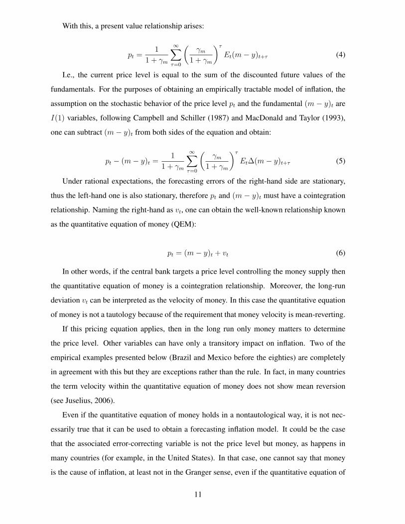
With this, a present value relationship arises:

pt =1

1 + γm

∞∑τ=0

(γm

1 + γm

)τ

Et(m− y)t+τ (4)

I.e., the current price level is equal to the sum of the discounted future values of the

fundamentals. For the purposes of obtaining an empirically tractable model of inflation, the

assumption on the stochastic behavior of the price level pt and the fundamental (m− y)t are

I(1) variables, following Campbell and Schiller (1987) and MacDonald and Taylor (1993),

one can subtract (m− y)t from both sides of the equation and obtain:

pt − (m− y)t =1

1 + γm

∞∑τ=0

(γm

1 + γm

)τ

Et∆(m− y)t+τ (5)

Under rational expectations, the forecasting errors of the right-hand side are stationary,

thus the left-hand one is also stationary, therefore pt and (m − y)t must have a cointegration

relationship. Naming the right-hand as vt, one can obtain the well-known relationship known

as the quantitative equation of money (QEM):

pt = (m− y)t + vt (6)

In other words, if the central bank targets a price level controlling the money supply then

the quantitative equation of money is a cointegration relationship. Moreover, the long-run

deviation vt can be interpreted as the velocity of money. In this case the quantitative equation

of money is not a tautology because of the requirement that money velocity is mean-reverting.

If this pricing equation applies, then in the long run only money matters to determine

the price level. Other variables can have only a transitory impact on inflation. Two of the

empirical examples presented below (Brazil and Mexico before the eighties) are completely

in agreement with this but they are exceptions rather than the rule. In fact, in many countries

the term velocity within the quantitative equation of money does not show mean reversion

(see Juselius, 2006).

Even if the quantitative equation of money holds in a nontautological way, it is not nec-

essarily true that it can be used to obtain a forecasting inflation model. It could be the case

that the associated error-correcting variable is not the price level but money, as happens in

many countries (for example, in the United States). In that case, one cannot say that money

is the cause of inflation, at least not in the Granger sense, even if the quantitative equation of

11

money holds. However, under the assumption that the central bank targets the price level and

uses money as its instrument, the error-correcting variable must be the price level and money

should be useful to forecast inflation. This is the case in other examples shown below but not

the rule in modern economies.

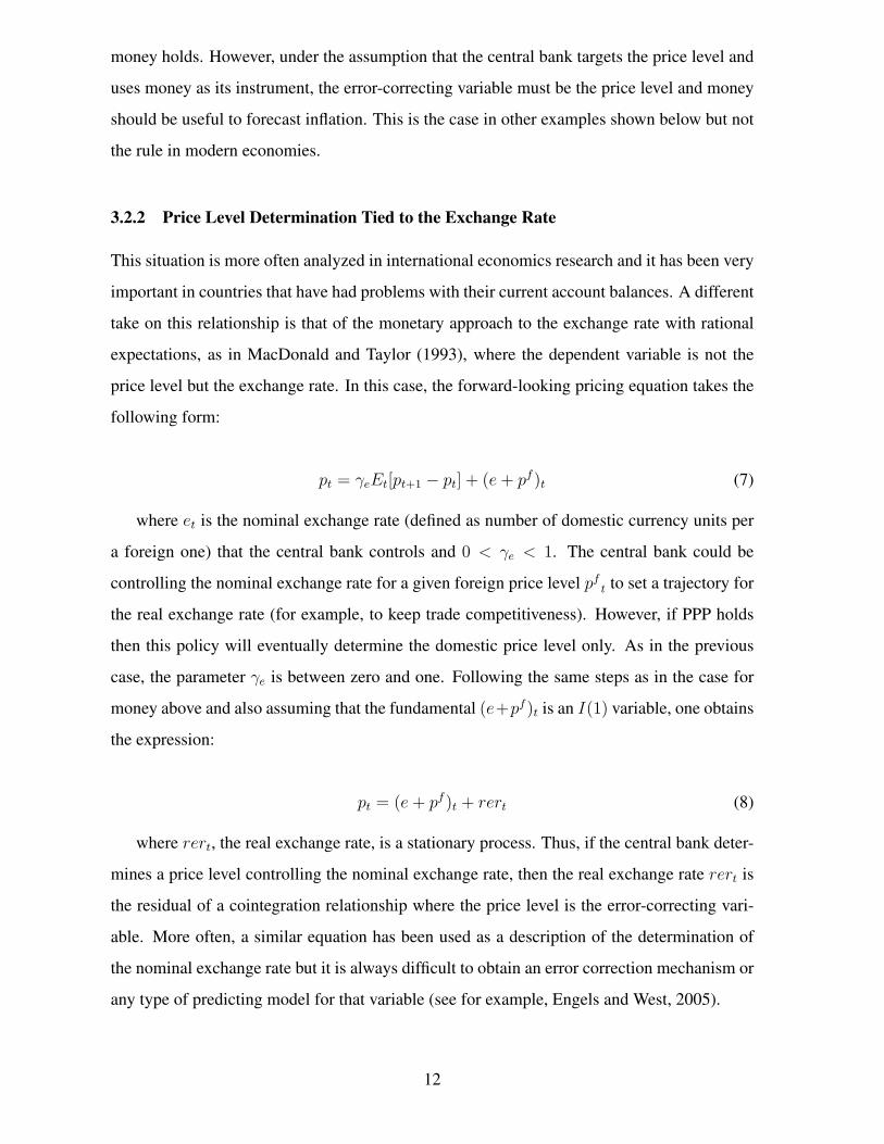
3.2.2 Price Level Determination Tied to the Exchange Rate

This situation is more often analyzed in international economics research and it has been very

important in countries that have had problems with their current account balances. A different

take on this relationship is that of the monetary approach to the exchange rate with rational

expectations, as in MacDonald and Taylor (1993), where the dependent variable is not the

price level but the exchange rate. In this case, the forward-looking pricing equation takes the

following form:

pt = γeEt[pt+1 − pt] + (e+ pf )t (7)

where et is the nominal exchange rate (defined as number of domestic currency units per

a foreign one) that the central bank controls and 0 < γe < 1. The central bank could be

controlling the nominal exchange rate for a given foreign price level pf t to set a trajectory for

the real exchange rate (for example, to keep trade competitiveness). However, if PPP holds

then this policy will eventually determine the domestic price level only. As in the previous

case, the parameter γe is between zero and one. Following the same steps as in the case for

money above and also assuming that the fundamental (e+pf )t is an I(1) variable, one obtains

the expression:

pt = (e+ pf )t + rert (8)

where rert, the real exchange rate, is a stationary process. Thus, if the central bank deter-

mines a price level controlling the nominal exchange rate, then the real exchange rate rert is

the residual of a cointegration relationship where the price level is the error-correcting vari-

able. More often, a similar equation has been used as a description of the determination of

the nominal exchange rate but it is always difficult to obtain an error correction mechanism or

any type of predicting model for that variable (see for example, Engels and West, 2005).

12

3.2.3 Inflation Rate Determination Tied to Economic Activity

Modern inflation rate targeting can be explicit, as in many economies, or implicit (for example,

in the United States before 2012). The target is achieved throughout the determination of

an interest rate that affects aggregate demand through different channels. In that approach

to monetary policy, the dominant model of inflation is the Phillips curve, particularly in its

forward-looking version, which is a fundamental ingredient of the New Keynesian theory of

business cycles. The forward-looking pricing equation takes the following form:

∆pt = γyEt[∆pt+1] + hy(yt − y∗t ) (9)

where yt and y∗t are the levels of actual and potential output, thus their difference is the

output gap while 0 < γy < 1 and hy are constants. The central bank cannot determine directly

the output gap or other measures of economic slack. It must do it indirectly through the policy

interest rate, which impacts the spending decisions of firms and consumers. This is known as

conventional monetary policy but in some circumstances, as when the short-run interest rate

is at or near the zero lower bound, the central bank might use unconventional measures such

as quantitative easing and credit easing. The (rational) expectations term allows a short-run,

but not a long-run trade-off between the output gap and inflation. Other variables stationary

might be included. The forward solution of equation (9) is the following:

∆pt = hy

∞∑τ=0

γτyEt(y − y∗)t+τ (10)

This means that current inflation depends on the stream of future output gaps, which are

proxies for marginal costs, as has often been pointed out in modern literature (Goodfriend and

King, 2009). These authors consider a more general model than the one used by Woodford

(2008). They assume that inflation contains a stochastic trend. This is necessary for the US

economy, where the price level appears to be an I(2) process, at least before the beginning of

the Great Moderation, which started more or less since the mid eighties. With trend inflation,

the solution is:

∆pt = ∆pt + hy

∞∑τ=0

γτyEt(y − y∗)t+τ (11)

where ∆pt is trend inflation. Of course, a more complete model has to specify a monetary

rule, an Euler equation and some other components as in Woodford (2007) and Goodfriend

13

and King (2009). Such elements, although necessary for a more complete picture of the

economy, are not indispensable to examine the inflation forecasting performance of models

based on slack measures of economic activity (see, for example, Stock and Watson, 2007 and

Faust and Wright, 2013).

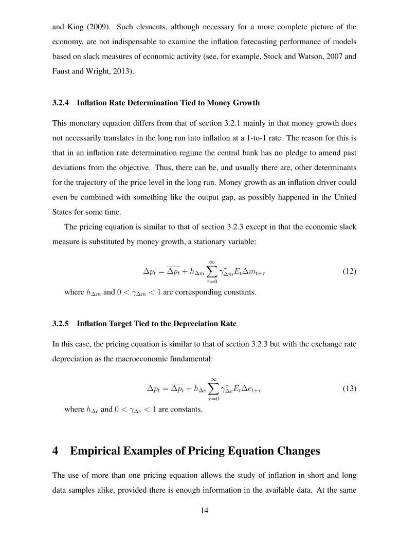
3.2.4 Inflation Rate Determination Tied to Money Growth

This monetary equation differs from that of section 3.2.1 mainly in that money growth does

not necessarily translates in the long run into inflation at a 1-to-1 rate. The reason for this is

that in an inflation rate determination regime the central bank has no pledge to amend past

deviations from the objective. Thus, there can be, and usually there are, other determinants

for the trajectory of the price level in the long run. Money growth as an inflation driver could

even be combined with something like the output gap, as possibly happened in the United

States for some time.

The pricing equation is similar to that of section 3.2.3 except in that the economic slack

measure is substituted by money growth, a stationary variable:

∆pt = ∆pt + h∆m

∞∑τ=0

γτ∆mEt∆mt+τ (12)

where h∆m and 0 < γ∆m < 1 are corresponding constants.

3.2.5 Inflation Target Tied to the Depreciation Rate

In this case, the pricing equation is similar to that of section 3.2.3 but with the exchange rate

depreciation as the macroeconomic fundamental:

∆pt = ∆pt + h∆e

∞∑τ=0

γτ∆eEt∆et+τ (13)

where h∆e and 0 < γ∆e < 1 are constants.

4 Empirical Examples of Pricing Equation Changes

The use of more than one pricing equation allows the study of inflation in short and long

data samples alike, provided there is enough information in the available data. At the same

14

time, it simplifies the construction of forecasting models by selecting variables that are the

most adequate for each period. This section analyzes four cases, one for a short sample, the

German hyperinflation (1921-1923) and three for long samples. First, the analysis is applied

to the cases of Mexico (1932-2013) and Brazil (1960-2013) not only because they are also

examples of the work of price level determination systems but because they used different

instruments to achieve their goals and finally adopting an inflation target system. The case

of the United States (1880-2007) is the best known, but there are some aspects about it that

are not frequently stressed. One of them is the changes in Granger causality, that is here

documented.

4.1 The German Hyperinflation (1921-1923)

This is an event where the sample is short but, given the very large rates of growth of mon-

etary variables and the speed of adjustment to shocks, it contains a lot of information about

monetary relationships and it has been a widely used case to study different aspects of money

demand, inflation and the exchange rate.

Hyperinflation has typically been seen as a convincing proof that inflation is ultimately

a monetary phenomenon in the sense that money drives the price level. However, Sargent

and Wallace (1973), among others, noted that money growth did not Granger-caused inflation

during the hyperinflations after World War I (WWI) but, instead, it was inflation the variable

that Granger-caused monetary growth. To make the monetary aggregate the economic cause

of inflation, they proposed a mechanism that involves increasing government spending which

demands growing amounts of money, and hence higher inflation, to finance it. If the price set-

ters have rational expectations then inflation leads money growth. As a follow up to this idea,

Makinen and Woodward (1988) found that after the price stabilization period that followed

six cases of after-WWI hyperinflations, among them the German one, the Granger causality

from prices to money vanished. Because of the Sargent and Wallace’s arguments, changes in

Granger causality have had a secondary or irrelevant role in the validation of inflation models.

The approach of this paper is different in that it considers those changes a relevant part

of what a monetary regime switch brings and not only in hyperinflation episodes. Thus, an

alternative explanation to the causality among monetary variables during the German hyperin-

flation is implicit in Bresciani-Turroni (1968). He divided the period in several stages, related

15

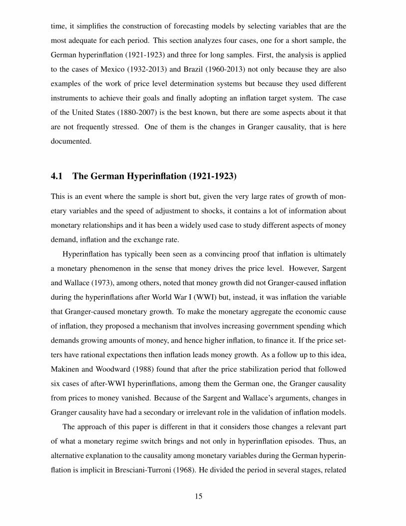
Figure 1: Exchange Rate Depreciation, Inflation and Money Growth In German Hyperinfla-

tion

to the German government’s demand of foreign currency to meet war reparations. In his di-

agram I, “volume of circulation” (currency) and “domestic prices” had a closer relationship

than that between domestic prices and the paper-marks-per-dollar exchange rate. In fact, un-

til just before the beginning of the hyperinflation period (July 2021), the exchange rate only

appeared correlated with the “prices of import goods” (diagrams III and IV). From May 1921

to the end of the hyperinflation in December 1923 (diagrams VI and VII), the relationship

between domestic prices and the exchange rate became very tight, as Figure 1 shows.

Thus, Bresciani-Turroni was in fact chronicling the substitution of one pricing equation

for another in which the driving cause was the need for foreign currency. This is actually a

balance of payment problem and it matches a situation that had been recognized as early as

the XVIII century, during the Swedish bullion controversy (Moosa and Towadros, 1999) and

has been present in many other cases, two of them examined below.

Figure 1 shows the time path of inflation, money growth and the depreciation rate for this

episode. It can be seen that since June 1921 on, money growth is led by both inflation and

the depreciation rate. It is also seen that inflation and the exchange rate depreciation are more

tightly correlated. The correlation between the first difference of these two variables is 0.92

while those of money growth with either of them is 0.5. This suggests that the exchange rate

and the price level were determined more or less simultaneously. This will be made more

precise later.

These impressions are confirmed by the following econometric analysis based on the ap-

16

proach of Garces-Diaz (2016), who applied it to a group of Latin American economies. First,

it must be said that the approach followed for the case of the German hyperinflation differs

from the other three cases because it is a typical case where cointegtration must be applied.

For Brazil and Mexico a similar analysis is carried out in Garces-D´az (2016). For the United

States, such approach cannot be applied because there is no evidence that country ever fol-

lowed a policy of price level determination. Therefore, a simpler Granger causality VAR

analysis is carried out for the last three cases.

Some definitions are needed here before discussing the econometric results. When there

are cointegration relationships in a model with nonstationary variables one can distinguish two

kinds of Granger causality. If the short-term shocks, for example lags of the changes of some

variables or any other stationary terms in the model help to forecast a different variable then

there is short-run Granger causality. However, in a cointegration system there is another way

in which one variable can be forecast on the basis of others. This is through the impact of the

error correction term where those other variables might be present. In this case, there is long-

run Granger causality, also known sometimes as “cointegrating causality,” going from the

nonstationary variables in the error correction term to the variable being forecast (Hatanaka,

1996, pp. 237-8). Long-run Granger causality is closely related to weak exogeneity, a concept

introduced by Engle et al. (1983):

“...a variable z, in a model is defined to be weakly exogenous for estimating

a set of parameters λ if inference on λ conditional on zt involves no loss of in-

formation. Heuristically, given that the joint density of random variables (yt,zt)

always can be written as the product of yt conditional on zt, times the marginal

of zt, the weak exogeneity of zt, entails that the precise specification of the latter

density is irrelevant to the analysis, and, in particular that all parameters which

appear in this marginal density are nuisance parameters.”

This is a general definition of weak exogeneity that when applied to the case of a coin-

tegrated system is stated as follows: “...a variable is weakly exogenous for the cointegrat-

ing parameters if none of the cointegration relations enter the equation for that variable.”

(Lutkepohl, 2004). Thus, in a cointegrated system a variable is weakly exogenous if it is

not Granger-caused in the long run by the other nonstationary variables. In other words, the

long-run causality must exist in only one direction, from the weakly exogenous variable to the

17

others that do not have this property. Notice that the property is maintained even if short-run

Granger causality runs in the other direction. Moreover, Engle et al. (1983) define a variable

as strongly exogenous if it is weakly exogenous (or, equivalently, not Granger-caused in the

long run) and it is not Granger-caused in the short run either. One should remember that

when both concepts, weak and strong exogeneity, are applied to linear models they become

equivalent to the more traditional ones of predeterminess and strict exogeneity (Killian and

Lutkepohl, 2017, ch. 7).

With this in mind one can analyze the German hyperinflation episode. The following

error-correction mechanisms show that the exchange rate and not the money supply was the

forcing variable during this period. Also, unbalanced regressions derived from the monetary

model show that the circulant was the only variable that was Granger-caused by the others by

it did not caused them, i.e., it was determined by the price level which in turn was determined

by the exchange rate.

Given that the number of observations is relatively small and, more to the point, it spans

less than three years, there are some issues that must be addressed related to the validity of the

results. It turns out, that neither of this characteristics of the sample are a matter of concern.

The reasons are two. First, there is not a number of observations that can be regarded as

minimum for the test to be valid. The reason is that, as discussed before, for the parameters to

be rightly estimated is necessary that there is enough information within the sample. This is

similar to the case discussed in Campos and Ericsson (1999), who use only 16 years of annual

data to estimate a model with five parameters for consumption expenditures in Venezuela for

the period 1970-1985. They argue that each observation is highly informative because the

variability is very high. In the case of the hyperinflation episodes the situation is similar and

the speed of adjustment is so high that the around 30 months used are enough to estimate the

models below. This is in fact a way to define a long-run relationship: the period that a system

takes to absorb a shock. If the speed of adjustment is high enough, as it is in the case here

analyzed, then the long-run happens in a short span of calendar time.

The first hypotheses to test are related to the role of the exchange rate in the determination

of the other nominal variables. As discussed above, the demand for foreign currency to pay

the war reparations was one of the most pressing matters for the Weimar Republic budget.

Thus, one would expect that this fact was reflected in the behavior of the nominal sector. In

particular, the exchange rate should be a weakly exogenous variable with respect to the price

18

level and the amount of currency, according to what Bresciani-Turroni (1968) observed. In

this case, in an equation for the exchange rate with dependent variable ∆et−1, there would be

no feed back from the price level. For this to happen, the variable et−1 should be statistically

nonsignificant in an unrestricted error correction mechanism. Thus, the null hypothesis in

the equation is that the coefficient for et−1 is equal to zero, using the proper critical values

for this kind of models. On the contrary, in the equation for ∆pt−1, the lagged variable

level of the price level pt−1 must be statistically different from zero with the hypothesis also

evaluated with the proper distribution. Also, in a cointegration system for the exchange rate

and currency, in the the unrestricted error correction model for ∆et−1, the coefficient for

et−1 should be statistically not different from zero. But is there is cointegration, then in the

unrestricted error correction model for ∆mt−1 the coefficient for the variable mt−1 should be

different from zero.

Table 1 shows the estimates for the four error correction models mentioned above. Only in

two of them the key parameter is significant. The first two are for the pair exchange rate and

the price level (et, pt) and the other two are for the exchange rate and the circulant (et,mt).

From the appropriate estimated parameters, one can infer which the leading variable was for

the nominal system during this period. The four models take the form of unconstrained error

correction mechanisms, one for each pair of the variables here considered. The regression

constants are not reported. The null hypothesis are described at the end of table.

For each model, the chief parameter corresponds to the lagged level of the variable which

is the dependent one in the form of first difference. The highlighted cells in Table 1 contain

the corresponding estimates of those parameters. The distribution of the t statistics for them

is nonnormal. Tables for the critical values for this kind of models are provided by Ericsson

and MacKinnon (2002). From their Table 3, one obtains the critical values. The first key

parameter, that for et−1 when the dependent variable is ∆et, has a positive sign when it is

required to be negative, as in any unrestricted error correction models. If one introduces as

a regressor the contemporary value for the rate of inflation ∆pt, then one obtains the right

sign for the estimate, which is -0.26. However, even in that case, the t statistics at -1.41 is far

below the critical value of 10 percent of significance which is -3.37. With such value for the t

statistic, one can infer that the price level is not a weakly exogenous variable for the exchange

rate thus, the contemporary value of the rate of inflation cannot be used in a regression as an

explanatory variable for the exchange rate. That is why the contemporary rate of inflation is

19

Table 1: Relationships of the Exchange Rate with the Price Level and the Circulant During

the German Hyper-inflationRelated variables

e, p e,mRegressors Dep. Var. Dep. Var.

∆et ∆pt ∆et ∆mt

et−1 0.64 0.56 -0.42 0.17(1.95) (5.76) (-2.47) (5.09)

pt−1 -0.56 -0.56 n.i. n.i.(-1.64) (-5.76) · ·

mt−1 n.i. n.i. 0.83 -0.19· · (3.74) (-4.81)

∆et n.i. 0.74 n.i. n.s.· (15.17) · ·

∆et−1 0.36 n.s. 0.86 n.s.(2.69) · (1.89) ·

∆pt−1 n.s. 0.22 n.i. n.i.· (5.84) · ·

∆mt n.i. n.i. n.i. n.i.· · · ·

∆mt−1 n.i. n.i. n.s. 0.32· · · (1.93)

dJul23 n.i. -0.80 n.i. n.i.· (-6.90) · ·

dOct23 3.46 0.90 n.i. n.i.(7.43) (4.41) · ·

Period 21:03-23:11 21:03-23:11 21:04-23:11 21:03-23:05

T 33 33 33 27Adjusted R2 0.89 0.99 0.83 0.89S.E. 0.42 0.10 0.51 0.06Jarque-B 0.09 0.33 0.71 0.59LM(2) autocor 0.80 0.21 0.66 0.07LM(1) ARCH 0.86 0.63 0.28 0.58t statistics are between parentheses.

The null hypothesis Ho in each case is that the coefficient in the shaded area is nondifferent from zero.

n.s. means excluded for being nonsignificant.

For Jarque-B, LM(2) autocor LM(2) ARCH the p values are provided.

20

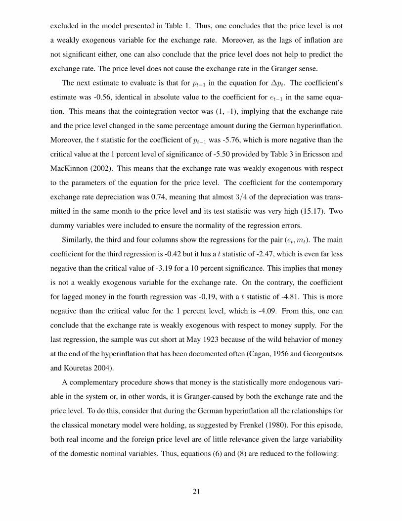
excluded in the model presented in Table 1. Thus, one concludes that the price level is not

a weakly exogenous variable for the exchange rate. Moreover, as the lags of inflation are

not significant either, one can also conclude that the price level does not help to predict the

exchange rate. The price level does not cause the exchange rate in the Granger sense.

The next estimate to evaluate is that for pt−1 in the equation for ∆pt. The coefficient’s

estimate was -0.56, identical in absolute value to the coefficient for et−1 in the same equa-

tion. This means that the cointegration vector was (1, -1), implying that the exchange rate

and the price level changed in the same percentage amount during the German hyperinflation.

Moreover, the t statistic for the coefficient of pt−1 was -5.76, which is more negative than the

critical value at the 1 percent level of significance of -5.50 provided by Table 3 in Ericsson and

MacKinnon (2002). This means that the exchange rate was weakly exogenous with respect

to the parameters of the equation for the price level. The coefficient for the contemporary

exchange rate depreciation was 0.74, meaning that almost 3/4 of the depreciation was trans-

mitted in the same month to the price level and its test statistic was very high (15.17). Two

dummy variables were included to ensure the normality of the regression errors.

Similarly, the third and four columns show the regressions for the pair (et,mt). The main

coefficient for the third regression is -0.42 but it has a t statistic of -2.47, which is even far less

negative than the critical value of -3.19 for a 10 percent significance. This implies that money

is not a weakly exogenous variable for the exchange rate. On the contrary, the coefficient

for lagged money in the fourth regression was -0.19, with a t statistic of -4.81. This is more

negative than the critical value for the 1 percent level, which is -4.09. From this, one can

conclude that the exchange rate is weakly exogenous with respect to money supply. For the

last regression, the sample was cut short at May 1923 because of the wild behavior of money

at the end of the hyperinflation that has been documented often (Cagan, 1956 and Georgoutsos

and Kouretas 2004).

A complementary procedure shows that money is the statistically more endogenous vari-

able in the system or, in other words, it is Granger-caused by both the exchange rate and the

price level. To do this, consider that during the German hyperinflation all the relationships for

the classical monetary model were holding, as suggested by Frenkel (1980). For this episode,

both real income and the foreign price level are of little relevance given the large variability

of the domestic nominal variables. Thus, equations (6) and (8) are reduced to the following:

21

pt = mt + vt (14)

pt = et + rert (15)

These equations for the log levels of the variables do not imply any particular Granger

causality structure but they can be used to derive it. The first step consists in running a

regression of the rate of change of each variable against the lagged levels of the other two and

lags of the rate of change of the three variables. In Garces Diaz (2016, 2017) this was done

only for the rate of inflation as the dependent variable. These regressions are:

∆ et = βep p

et−1 + βe

mmt−1 + ϕep∆pt−1 + ϕe

m∆mt−1 (16)

∆ ppt = βpe et−1 + βp

mmt−1 + ϕpe∆et−1 + ϕp

m∆mt−1 (17)

∆mt = βme emt−1 + βm

p pt−1 + ϕme ∆et−1 + ϕm

p ∆ pt−1 (18)

Where the superscripts refer to the dependent variable and the subscripts to the regressors.

These are unbalanced regressions due to the fact that the integration order of the dependent

variable, which is in first difference, is lower than that of the regressors in levels. Because

of this, the t statistics for the coefficients with the higher order of integration cannot be an-

alyzed with standard inference. However, differently from what happens in the case when

there is one nonstationary regressor, which can generate a spurious relationship, as shown by

Granger and Newbold (1974), the presence of two nonstationary regressors helps to avoid this

problem, provided the correct distributions are used in the inference. As discussed in Pagan

and Wickens ( 1989), if the nonstationary regressors are unrelated to the dependent variable,

then their coefficients must be zero. If they form a valid cointegration relationship they form

a valid regression but with coefficients with a nonstandard distribution. This is done here

transforming the unbalanced regressions into unrestricted error correction models and use the

Ericsson and MacKinnon (2002) tables mentioned before.

The procedure is the following. First, when the monetary model does not work as pre-

scribed by theory, the coefficients for the nonstationary variables should be zero in all three

equations. So, this procedure is a simple way to test if the monetary model is working in a

given sample or not. Second, if the monetary model is truly working, the nominal variables

22

et, pt and mt can be used as proxies of one another. In principle, the estimates of those param-

eters should be very similar in absolute value because of the restrictions on the parameters of

the monetary model. The interesting part comes from the fact that if one regression is valid in

the sense that the nonstationary variables are statistically significant, and at least one must be

because otherwise there would be no cointegration, then the coefficients for the nonstationary

variables will have the signs reversed. The variable with negative sign takes the place of the

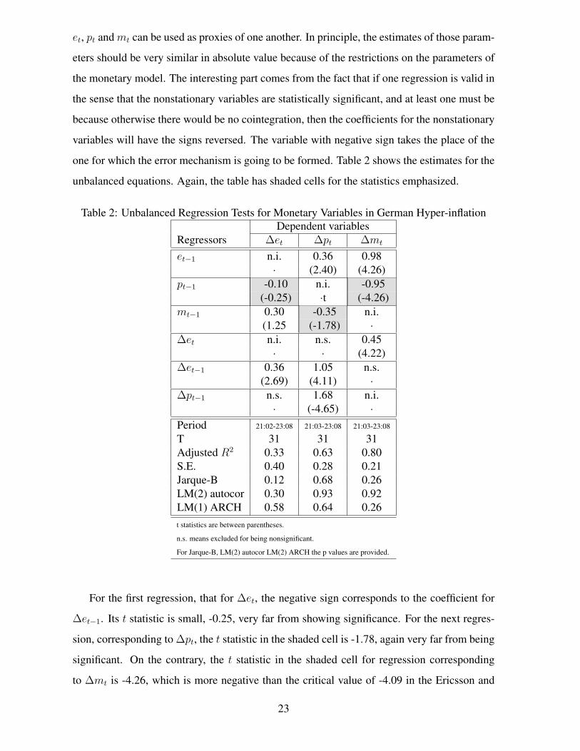
one for which the error mechanism is going to be formed. Table 2 shows the estimates for the

unbalanced equations. Again, the table has shaded cells for the statistics emphasized.

Table 2: Unbalanced Regression Tests for Monetary Variables in German Hyper-inflationDependent variables

Regressors ∆et ∆pt ∆mt

et−1 n.i. 0.36 0.98· (2.40) (4.26)

pt−1 -0.10 n.i. -0.95(-0.25) ·t (-4.26)

mt−1 0.30 -0.35 n.i.(1.25 (-1.78) ·

∆et n.i. n.s. 0.45· · (4.22)

∆et−1 0.36 1.05 n.s.(2.69) (4.11) ·

∆pt−1 n.s. 1.68 n.i.· (-4.65) ·

Period 21:02-23:08 21:03-23:08 21:03-23:08

T 31 31 31Adjusted R2 0.33 0.63 0.80S.E. 0.40 0.28 0.21Jarque-B 0.12 0.68 0.26LM(2) autocor 0.30 0.93 0.92LM(1) ARCH 0.58 0.64 0.26t statistics are between parentheses.

n.s. means excluded for being nonsignificant.

For Jarque-B, LM(2) autocor LM(2) ARCH the p values are provided.

For the first regression, that for ∆et, the negative sign corresponds to the coefficient for

∆et−1. Its t statistic is small, -0.25, very far from showing significance. For the next regres-

sion, corresponding to ∆pt, the t statistic in the shaded cell is -1.78, again very far from being

significant. On the contrary, the t statistic in the shaded cell for regression corresponding

to ∆mt is -4.26, which is more negative than the critical value of -4.09 in the Ericsson and

23

MacKinnon table 3. It is also important to notice that the absolute values for the coefficients

of et−1 and pt−1 in that regression, 0.98 and 0.95 respectively, are very similar. This is because

as shown in the previous table the exchange rate and the price level are cointegrated with co-

efficients (1,-1). For these equations, the sample was shortened to the first half of 1923, as has

been common practice in models on the German hyperinflation (as, for example, in Cagan’s

classical paper) because during the second part of 1923, money growth behaved wildly, in a

way that has resisted a clear explanation within a model.

Thus, during the German hyperinflation, the pricing equation working was really (7) and

not (1), as is often stated. In other words, there was an implicit price level determination

regime with the exchange rate rather than money as the driving variable. Of course, this does

not contradict that people were expecting increases in the money supply after rising prices.

Money can be very well the final cause of inflation but there is at least a practical relevance in

asking in general terms why is that Granger causality varies according to the monetary regime.

This is best exemplified looking at two cases that share several similarities and are not pure

cases of hyperinflation. Indeed, the approach applied to the German hyperinflation can be

applied to any case regardless of the level of inflation provided there is enough information in

the sample.

4.2 Mexico (1932-2013)

A cointegration analysis for Mexico and Brazil similar to that applied to the German hyperin-

flation episode is carried out in Garces-Dıaz (2016) but here an alternative approach is taken.

This can also be applied to the cases when the inflation rate is determinated instead of the price

level, something where the concept of cointegration is appropriate. However, as the variables

involved contain stochastic trends, regular Granger causality tests might not be applicable be-

cause the covariance matrix of the joint distribution of the VAR parameters is singular (Killian

and Lutkepohl, 2017). However, Toda and Yamamoto (1995) showed that there is a simple

solution to this problem. This consists in adding an additional lag to the VAR process fitted to

the data for each degree of integration of the series after the optimal number of lags has been

determined. This produces a nonsingular covariance matrix for the parameters related to the

lags optimally determined. The Wald test is then applied to the optimal number of lags alone

ignoring the additional ones arising from the integration of the series.

24

The Toda-Yamamoto test can account for both long-run and short-run Granger causality

but it cannot distinguish between them. When there is long-run causality, then the series must

be cointegrated, as discussed above, but the converse is not true. In the cases of Mexico and

Brazil, for most of the sample there was price-level determination and cointegration, as shown

in Garces Dıaz (2016). However, when both countries adopted inflation targeting, there is no

long-run causality so the test indicates the presence or absence of short-run causality. In the

case of the United States there is no evidence of price level determination. Only Sweden,

among all developed countries, experienced with it during a brief period, as mentioned be-

fore. Thus one must consider that in the cases of Mexico and Brazil, the Toda-Yamamoto

tests confirm the evidence of long-run Granger causality for the respective subsample. In the

case of the United States, the result must be interpreted as evidence of short-run causality.

These are the tests applied below. As the data periodicity is annual and it is in turn divided

into subsamples (regimes), there is a constrain to the number of lags one can include in the

corresponding VARs. This is critical because some of the criteria suggests more than one lag

and there is an ambiguity on the degree of integration of the time series, as shown in Garces

Dıaz (2016). Because of this, all of the VARs are run with two lags plus an additional one that

covers the degree of integration of all the series that will be presumed to be one despite that

ambiguity.

The Mexican case produces the clearest application of the hypothesis of simultaneous

changes in pricing equations and Granger causality. The country is usually included in the

high inflation category (for example, Jones 2011), but it has a more complex and interesting

story than that. It actually had an episode of low inflation, virtually identical in average to that

of the US (1956 to 1971). Low inflation was again the norm since 2001 onwards. Its highest

level of annual inflation was 99 percent in 1987 although it had a month of 12-month inflation

of 150 per cent in 1988. The country has applied several types of exchange rate systems. Most

interesting, the theoretical monetary relationships, for example PPP and the QEM, appear in

its data with stunning clarity for much of the sample.

In Mexico’s case, it is easy to find the dates of change for the pricing equation and Granger

causality because there were well-known public events that signaled them. The first episode

goes from 1932, when the country like many others abandoned the Gold standard, to 1981.

In this long span, the central bank had as an objective to maintain the stability of the nominal

exchange rate, despite several devaluations. This required to implicitly determine the price

25

level, which was tied to the level of currency even though there was no explicit official state-

ment of doing so. Thus, for this period, the pricing equation at work was (1). The implications

of that were that the QEM held and that money Granger-caused the price level.

In 1982, Mexico looked for financial assistance from the IMF. In the agreement with that

institution, there were two key provisions that propelled a change in the price equation. First,

the central bank could not longer provide financing for the public deficit through primary

emission of money. Second, the IMF recommended a policy of competitive devaluations.

This shifted the attention of the price setters from money to the exchange rate as the the

central bank’s instrument to drive the price level. As in the previous regime, this was never

stated as an official objective but the behavior of the price level was better described with a

price level determination regime. Thus, since 1983 to 2003, the price equation was (13). This

changed the Granger causality structure among the variables. Interestingly enough, the year

1982 as period of transition does not fit well in any of the two regimes. A similar transition

period happens also in the case of Brazil, described next.

At the end of the 1990s, the Mexican central bank announced its intention to apply an

inflation targeting regime. This was a big change because for the first time since its foundation

in 1925, it was attempting to abandon any kind of policy setting better that could be described

with a price level determination pricing equation. This caused that the new price equation had

the form (9). This again caused a change in the Granger causality structure. Since then, both

the exchange rate and money aggregates ceased to Granger-cause inflation.

The changes in Granger causality can be appreciated in Table 3, which contains the Toda-

Yamamoto (1995) tests for Granger Causality for nonstationary data to the log levels of the

price level (pt), money (mt) and the exchange rate (et) organized by pairs and in different

regimes. However, as happens in the United States and many other economies, simple corre-

lations between the output gap, or other measures of economic activity, are not easy to get.

A possible reason for this, besides perhaps not being closely related as some economists sug-

gest, is provided in the discussion for the United States below: for the first time, Mexico and

the United States had similar pricing equations.

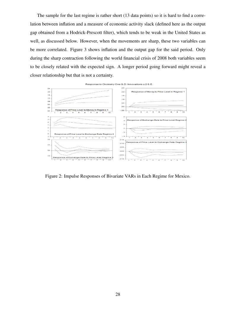
There are several alternatives of impulse-response functions for these VARs. Figure 2

shows the impulse-response functions for pairs of the first differences in monetary variables

for the three regimes determined by different pricing equations. These confirm the structure

of Granger causality for each regime. Similar results are obtained with VARs in levels and

26

Table 3: Mexico: Bivariate Granger Causality Tests For Nonstationary Variables in Each

Regime

Dependent Variable: Price Level pt

Regime 1 Regime 2 Regime 3

Excluded Variable χ2(2) p-value χ2(2) p-value χ2(2) p-value

Inflationary Money (m− y)t 9 .73 0 .01 2 .27 0 .32 0 .26 0 .88

Exchange Rate et 2 .17 0 .34 7 .02 0 .03 3 .43 0 .18

Dependent Variable: Inflationary Money (m− y)t

Regime 1 Regime 2 Regime 3

Excluded Variable χ2(2) p-value χ2(2) p-value χ2(2) p-value

Price Level pt 1 .73 0 .42 15 .89 0 .00 2 .14 0 .34

Exchange Rate et 1 .52 0 .22 11 .80 0 .00 0 .23 0 .63

Dependent Variable: Exchange Rate et

Regime 1 Regime 2 Regime 3

Excluded Variable χ2(2) p-value χ2(2) p-value χ2(2) p-value

Price Level pt 2 .23 0 .33 1 .56 0 .46 1 .23 0 .54

Inflationary money (m− y)t 7 .57 0 .01 0 .26 0 .61 2 .46 0 .11

The test was modified following Toda and Yamamoto (1995).

The Wald test statistic is distributed as a χ2(2).

also imposing cointegration restrictions. Actually, in this case is possible to construct infla-

tion models for each regime based on the long-run relationships and their respective error-

correction mechanisms. They provide good forecasting performance out of sample, as shown

in Garces Dıaz (2016).

However, the property of switching Granger causality makes this a more complex task

than usual because most cointegration tests methods are based on the assumption of invariant

Granger causality or, equivalently, the constancy of the feedback parameters. In a companion

paper (Garces Dıaz 2016), this procedure is described for Mexico and other five major Latin

American Economies. The equations obtained for Mexico are an error-correction model based

on money for the period 1932-1981; an error-correction model based on the exchange rate for

the 1983-2000 sample and; a model of noise for the period 2001-2013.

27

The sample for the last regime is rather short (13 data points) so it is hard to find a corre-

lation between inflation and a measure of economic activity slack (defined here as the output

gap obtained from a Hodrick-Prescott filter), which tends to be weak in the United States as

well, as discussed below. However, when the movements are sharp, these two variables can

be more correlated. Figure 3 shows inflation and the output gap for the said period. Only

during the sharp contraction following the world financial crisis of 2008 both variables seem

to be closely related with the expected sign. A longer period going forward might reveal a

closer relationship but that is not a certainty.

Figure 2: Impulse Responses of Bivariate VARs in Each Regime for Mexico.

28

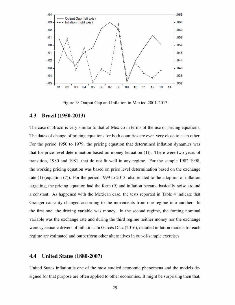
Figure 3: Output Gap and Inflation in Mexico 2001-2013

4.3 Brazil (1950-2013)

The case of Brazil is very similar to that of Mexico in terms of the use of pricing equations.

The dates of change of pricing equations for both countries are even very close to each other.

For the period 1950 to 1979, the pricing equation that determined inflation dynamics was

that for price level determination based on money (equation (1)). There were two years of

transition, 1980 and 1981, that do not fit well in any regime. For the sample 1982-1998,

the working pricing equation was based on price level determination based on the exchange

rate (1) (equation (7)). For the period 1999 to 2013, also related to the adoption of inflation

targeting, the pricing equation had the form (9) and inflation became basically noise around

a constant. As happened with the Mexican case, the tests reported in Table 4 indicate that

Granger causality changed according to the movements from one regime into another. In

the first one, the driving variable was money. In the second regime, the forcing nominal

variable was the exchange rate and during the third regime neither money nor the exchange

were systematic drivers of inflation. In Garces Dıaz (2016), detailed inflation models for each

regime are estimated and outperform other alternatives in out-of-sample exercises.

4.4 United States (1880-2007)

United States inflation is one of the most studied economic phenomena and the models de-

signed for that purpose are often applied to other economies. It might be surprising then that,

29

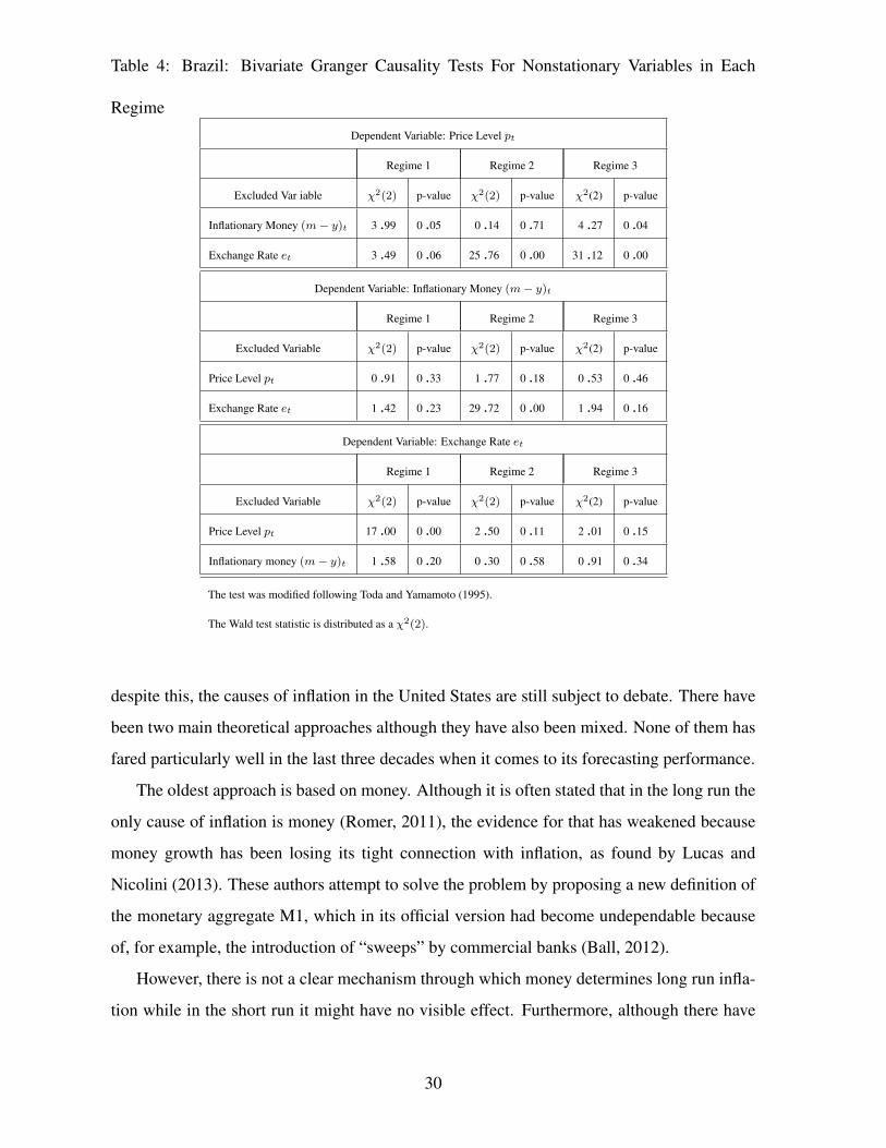
Table 4: Brazil: Bivariate Granger Causality Tests For Nonstationary Variables in Each

Regime

Dependent Variable: Price Level pt

Regime 1 Regime 2 Regime 3

Excluded Var iable χ2(2) p-value χ2(2) p-value χ2(2) p-value

Inflationary Money (m− y)t 3 .99 0 .05 0 .14 0 .71 4 .27 0 .04

Exchange Rate et 3 .49 0 .06 25 .76 0 .00 31 .12 0 .00

Dependent Variable: Inflationary Money (m− y)t

Regime 1 Regime 2 Regime 3

Excluded Variable χ2(2) p-value χ2(2) p-value χ2(2) p-value

Price Level pt 0 .91 0 .33 1 .77 0 .18 0 .53 0 .46

Exchange Rate et 1 .42 0 .23 29 .72 0 .00 1 .94 0 .16

Dependent Variable: Exchange Rate et

Regime 1 Regime 2 Regime 3

Excluded Variable χ2(2) p-value χ2(2) p-value χ2(2) p-value

Price Level pt 17 .00 0 .00 2 .50 0 .11 2 .01 0 .15

Inflationary money (m− y)t 1 .58 0 .20 0 .30 0 .58 0 .91 0 .34

The test was modified following Toda and Yamamoto (1995).

The Wald test statistic is distributed as a χ2(2).

despite this, the causes of inflation in the United States are still subject to debate. There have

been two main theoretical approaches although they have also been mixed. None of them has

fared particularly well in the last three decades when it comes to its forecasting performance.

The oldest approach is based on money. Although it is often stated that in the long run the

only cause of inflation is money (Romer, 2011), the evidence for that has weakened because

money growth has been losing its tight connection with inflation, as found by Lucas and

Nicolini (2013). These authors attempt to solve the problem by proposing a new definition of

the monetary aggregate M1, which in its official version had become undependable because

of, for example, the introduction of “sweeps” by commercial banks (Ball, 2012).

However, there is not a clear mechanism through which money determines long run infla-

tion while in the short run it might have no visible effect. Furthermore, although there have

30

been many attempts to show that money demands are stable in both the long-run (Benati, et

al. 2016) and the short run (Ball, 2012), the procedures involved in these studies have ignored

the possibility of a regime changes that could be hidden by the dominance of some periods.

For example, Teles and Uhlig (2013) found for a large sample of countries that the relation-

ship between the price level and money has decreased considerably since the 1990s. As since

that period inflation has tended to become lower in most countries, its properties might be

dominated by previous episodes of higher and more variable inflation and money growth.

Because of that, it would be better to consider equation (6) as a more proper pricing

equation for the United States for the time when money had an effect on inflation, possibly

from 1880 to the 60s or seventies. For many years already, it has been stated that money is

not useful to forecast inflation in the United States as in the form of the P* model (Christiano,

1989).

A more recent and popular alternative is the Phillips curve, adopted since the sixties by

Keynesian economists as their pricing equation. According to Stock and Watson (2007), that

model was able to produce good inflation forecasts from 1970 to 1983. However, since the

outset of the Great Moderation (1984 to 2004 in their sample), they found that it had a dismal

performance. More recent work has confirmed this finding for later years. In particular, the

failure of the Phillips curve to forecast inflation after the 2008 economic crisis (“the miss-

ing deflation” puzzle) and the posterior recovery (“the missing inflation” puzzle) has been

widely commented. Some economists have expressed doubts that inflation in a stable eco-

nomic environment can really be tied to specific causes. For example, Hall (2011) suggested

to consider inflation as a “near-exogenous” process, echoing what many Keynesian models

from the 1950s to the early 1970s assumed (Woodford, 2008). Nevertheless, Del Negro et

al. (2015) made some modifications to the standard New Keynesian model and were able to

produce better forecasts for that event and following years. However, they did not address the

previous the problem of poor forecasting since the mid eighties.

Goodfriend and King (2009) provide an explanation for the lack of predictive power of

economic activity on inflation. They suggest that if the central bank stabilizes economic

activity in their “business as usual” practices, then inflation becomes determined only by

its trend and output gap or unemployment measures cannot be used to forecast it. When

the central bank actively attempts to control growing inflation by raising the interest rate

to slow economic activity, as the Fed did during the seventies and early eighties, slackness

31

measures have predictive power in inflation models. This explanation is consistent with what

was observed by Stock and Watson (2007).

Differently from other cases examined in this paper, the changes of regime in the United

States are harder to see because its macroeconomic variables are relatively not very volatile,

the information they contain is harder to extract. For example, Sims and Zha (2006) found

necessary to include money (M2), along the federal funds rate, to be able to identify the mon-

etary policy regimes that the Federal Reserve has followed . They argue that in the seventies,

monetary aggregates were part of the discussions of monetary policy.

Because of this, the date of change of one regime into another was chosen as follows.

There was a regime when money was tightly related to inflation from 1888, when the sample

starts, to 1983 when the connection between them began to diminish and the Great Moderation

was about to start. This separation of regimes revels that not only the correlation between

these variables weakened since the beginning of the eighties: Granger causality from money

growth to inflation also disappeared since the Great Moderation, as can be seen in Table 5. As

money grew faster since 2008 because of Federal Reserve’s quantitative easing, it is clear that

the causality has not been reestablished since then.

5 Conclusions

A promising approach to get a better understanding of inflation dynamics is to consider radical

regime changes of the pricing equation, not only in the parameters of a specific type. In other

words, one can ponder the possibility that the whole right-hand side of an inflation model

changes, including the explanatory variables and the functional form. This approach has been

somehow implicit in many studies. For example, for a period of hyperinflation there is one

type of pricing equation (for example, a monetarist one) that is replaced by another when

inflation is low (for example, a Keynesian one).

A first consideration is to explicitly decide if the monetary regime in place determines

either the price level or the inflation rate as this settles the issue of how persistent different

inflationary shocks are. Next, it is important to decide if the main objective of the monetary

authority is to maintain price stability or something else (for example, budget deficit financ-

ing). Then it is necessary to identify the drivers of inflation that can be regarded as systematic

32

Table 5: Trivariate Granger Causality Tests For US Inflation, M2 and GDP

Dependent Variable: Inflation ∆pt

1888-1983 1984-2007

Excluded Variable χ2(2) p-value χ2(2) p-value

Money Growth ∆mt 6 .86 0 .01 1 .37 0 .50

GDP Growth ∆yt 0 .17 0 .68 1 .01 0 .60

Dependent Variable: Money Growth ∆mt

1888-1983 1984-2007

Excluded Variable χ2(2) p-value χ2(2) p-value

Inflation ∆pt 1 .80 0 .18 1 .45 0 .48

GDP Growth ∆yt 0 .57 0 .45 11 .37 0 .00

Dependent Variable: GDP Growth ∆yt

1888-1983 1984-2007

Excluded Variable χ2(2) p-value χ2(2) p-value

Inflation ∆pt 2 .43 0 .12 3 .75 0 .15

Money Growth ∆mt 0 .06 0 .81 0 .92 0 .63

The test was modified following Toda and Yamamoto (1995).

The Wald test statistic is distributed as a χ2(2).

so one does not have to deal with many factors that, although they might be important at some

periods, it is not necessary they are always acting. Thus, one has to look carefully for the

variables that are the acting systematic inflationary factors at each point of time. By applying

that procedure, one has to give a central role to Granger causality and conditional forecasts

of inflation. A variable that has no predicting value for inflation is discarded as a systematic

cause of price changes. This approach solves several puzzles such as the declining contem-

porary and dynamic correlations of money growth, exchange rate movements and economic

slack measures with inflation.

During the German hyperinflation, money is Granger-caused by the price level and not

the other way around. This has been explained as a trick played by the rational expectations

of economic agents. However, there are cases, as those presented here, where the direction of

Granger causality is the opposite so currently there is at least an incomplete explanation for

what happens to Granger causality properties in one case or another. For Mexico and Brazil,

33

the Toda-Yamamoto tests show that there was change in the direction of Granger causality at

given dates, obtained through a review of historical events (for example, the announcement

of the adoption of inflation targeting). In both cases, the money stock was the driving force

behind price level movements. Then from around 1982 to the beginning of the 2000s, the

exchange rate was the driving cause behind the price level determination. In none of these

episodes the main concern of the central banks was price stability. However, since around the

beginning of the 2000s both countries adopted inflation targeting and the pass-through of both

money and exchange rate shocks on inflation were considerably diminished to tiny effects, if

any. For the United States there was also a change in Granger causality. Before the eighties,

money growth Granger caused inflation but since the mid eighties onwards, the causality

changed direction and money became of little use to predict inflation. This is consistent with

the dominance of cashless models of inflation in recent times.

Although the approach looks promising to solve some issues of the dynamics of infla-

tion, there are others that are left unanswered. The results for the United States shows that

identifying the direction of Granger causality is not enough to obtain a forecasting model

that beats simple time series models. An additional weakness is that the dates of the regime

changes have to be provided by the modeler. This seems to be a rather challenging problem

with no easy solution. Nonetheless, the approach seems worth trying with different data sets.

Among some projects, one can study general differences in the dynamics of inflation between

advanced and emerging economies. Another project is the application of the approach to the

data of some relevant papers on inflation models such as that of Hendry (2001 and 2015), who

uses many explanatory variables for inflation instead of the very few that are suggested in this

article.

References

[1] Ball, L. (2012), “Short-run money demand,” Journal of Monetary Economics, Volume

59, Issue 7, November, Pages 622633.

[2] Barro, R.J. (1979) “Money and the Price Level Under the Gold Standard,” The Economic

Journal, Vol. 89, No. 353 (March).

34

[3] Benati, L., Robert E. Lucas, Jr., Juan Pablo Nicolini, and Warren Weber (2016), “In-

ternational Evidence on Long Run Money Demand,” NBER Working Paper No. 22475,

July.

[4] Bobeica, E. and Marek Jarocinski (2017), “Missing disinflation and missing inflation:

the puzzles that arent,” European Central Bank Working Paper 2000, January.

[5] Bresciani-Turroni, C. (1968), “The Economics of Inflation,” 3rd. reim-

pression, John Dickens & Co. Ltd., Northampton. Available online in

http://mises.org/library/economics-inflation-study-currency-depreciation-post-war-

germany

[6] Cagan, P. (1956), “The Monetary Dynamics of Hyperinflation,” in Studies in the Quan-

tity Theory of Money, ed. by M. Friedman. University of Chicago Press, Chicago, IL.

[7] Campbell, J. Y., and Robert J. Shiller. (1987) “Cointegration and tests of present value

models.” Journal of Political Economy 95(5).

[8] Campos, J. and Neil R. Ericsson (1999), “Constructive data mining: modeling con-

sumers expenditure in Venezuela,” Econometrics Journal, volume 2, pp. 226240.

[9] Castle, J. and David F. Hendry (2007), “Forecasting UK Inflation: the Roles of Struc-

tural Breaks and Time Disaggregation,” Oxford University, Department of Economics,

Discussion Paper Series, No. 309.

[10] Christiano, L. J. (1989), “P*: Not the Inflation Forecaster’s Holy Grail,” Quarterly Re-

view, Federal Reserve Bank of Minneapolis, Fall, pp. 3-18.

[11] Citu, F.V. (2002) “Review of the literature on the comparison of price level targeting and

inflation targeting,” Federal Reserve Bank of New Zealand, Publications.

[12] Clements, M. P. and David F. Hendry (2008) “Forecasting Annual UK Inflation Using

an Econometric Model over 1875-1991,” in Forecasting in the Presence of Structural

Breaks and Model Uncertainty, Edited by David E. Rapach abd Mark E. Wohar.

[13] De Long, J. B. (1996) “America’s Only Peacetime Inflation: The 1970s,” NBER Histor-

ical Working Paper No. 84, May.

35

[14] Del Negro, M., Marc P. Giannoni, and Frank Schorfheide (2015), “Inflation in the

Great Recession and New Keynesian Models.” American Economic Journal: Macroe-

conomics, 7 (1): 168-96.

[15] Dotsey, M., Shigeru Fujita and Tom Stark (2017) “Do Phillips Curves Conditionally

Help to Forecast Inflation”, Federal Reserve Bank of Philadelphia, WP. No. 11-40.

[16] Engels, C. and Kenneth D. West (2005), “Exchange Rates and Fundamentals,” Journal

of Political Economy, vol 113, no. 3.

[17] Engle, R. F., David F. Hendry and Jean-Francois Richard (1983) “Exogeneity,” Econo-

metrica, Vol. 51, No. 2, pp. 277-304.

[18] Ericsson, N. R. and James G. Mackinnon (2002), “Distributions of error correction tests

for cointegration,” Econometrics Journal, v.5, pp285-318.

[19] Faust, J. and Jonathan H. Wright (2013) “Forecasting Inflation,” Handbook of Economic

Forecasting, Ch. 1, vol. 2, pp 2-56.

[20] Frenkel, J. (1980) “Exchange Rates, Prices, and Money: Lessons from the 1920’s,” in In-

terwar Macroeconomics From the Perspective of the 1970’s, May, American Economic

Association, pp 235-242.

[21] Friedman, M. (1987), “Quantity Theory of Money,” The New Palgrave Dictionary of

Economics, First Edition, Edited by John Eatwell, Murray Milgate and Peter Newman,

MacMillan.

[22] Garces Dıaz, D. G. (2016) “Changes in Inflation Predictability in Major Latin American

Countries,” Banco de Mexico, Documento de Investigacion No. 2016-20, December

2016.

[23] Garces Dıaz, D. G. (2017) “Explaining Inflation with a Classical Dichotomy Model and

Switching Monetary Regimes: Mexico 1932-2013,” Banco de Mexico, Documento de

Investigacion No. 2017-20, December 2017.

[24] Georgoutsos D. A. and Georgios P. Kouretas (2004), “A Multivariate I(2) cointegration

analysis of German hyperinflation,” Applied Financial Economics, 14:1, 29-41.

36

[25] Goodfriend, M. and Robert G. King (2009) “The Great Inflation Drift”, NBER Working

Paper No. 14862, April.

[26] Gordon, R.J. (2013) “The Phillips Curve is Alive and Well: Inflation and the NAIRU

During the Slow Recovery,” NBER Working Paper No. 19390 August 2013.

[27] Granger, C.W.J. and P. Newbold (1974) “Spurious Regressions in Economterics,” Jour-

nal of Econometrics 2, 111-120.

[28] Hall, R.E. (2002) “Controlling the Price Level”, Contributions to Macroeconomics, Vol-

ume 2, Issue 1, Article 5.

[29] Hall, R.E. (2011) “The Long Slump”, American Economic Review, 101 (April 2011):

431-469.

[30] Hall, T. E. and William R. Hart (2012) “The SamuelsonSolow Phillips Curve and the

Great Inflation,” History of Economics Review, Volume 55, 2012 - Issue 1.

[31] Hatanaka, M. (1996) “Time-Series-Based Econometrics: Unit Roots and Co-

Integrations,” Oxford University Press.

[32] Hendry, D. F. (2001), “Modelling UK inflation, 1875-1991”, Journal of Applied Econo-

metrics, v. 16, Issue 3, pp. 255-275.

[33] Hendry, D. F. (2015), “Introductory Macro-econometrics: A New Approach”, Timber-

lake Consultants Ltd.

[34] Hendry, D. F. and Neil R. Ericsson (1991), “An Econometric Analysis of U.K. Money

Demand in Monetary Trends in the United Statesand the United Kingdom by Milton

Friedman and Anna J. Schwartz,” The American Economic Review, Vol. 81, No. 1, pp.

8-38.

[35] Jones, C. I. (2011) “Macroeconomics,” Second Edition, W.W. Norton & Company.

[36] Jonung, L. (1979) “Knut Wicksell’s Norm of Price Stabilization and Swedish Monetary

Policy in the 1930s,” Journal of Monetary Economics, 5, 459-496.

[37] Juselius, K. (2006), “The Cointegrated VAR Model: Methodology and Applications”,

Advanced Texts in Econometrics, Oxford University Press.

37

[38] Killian, L. and Helmut Lutkepohl (2017), “Structural Vector Autoregressive Analysis,”

Cambridge University Press, 2017.

[39] Levy, D. (2002) “Cointegration in Frequency Domain,” Journal of Time Series Analysis

23.

[40] Lutkepohl, H. (2004) “Vector Autoregressive and Vector Error Correction Models,” in

Applied Time Series Econometrics, Lutkepohl and Markus Kratzig (ed), Cambridge Uni-

versity Press.

[41] Lucas, R.E. and Juan Pablo Nicolini (2013) “On the Stability of Money Demand”, Meet-

ing Papers 353, Society for Economic Dynamics.

[42] MacDonald, R. and Mark P. Taylor (1993) “The Monetary Approach to the Exchange

Rate: Rational Expectations, Long-Run Equilibrium, and Forecasting,” Staff Papers,

International Monetary Fund, Vol. 40, No. 1.

[43] Moosa, I. A. and George Towadros (1999), “The Monetary Model of Exchange Rates in

the History of Economic Thought”, History of Economics Review, Volume 29 - Issue 1.

[44] Makinen, G.E. and Thomas Woodward (1988), “The Transition from Hyperinflation to

Stability: Some Evidence,” Eastern Economic Journal, Vol. 14, No. 1, pp. 19-26.

[45] Pagan, A. R. and M. R. Wickens (1989), “A survey of some recent econometric meth-

ods,” Economic Journal 99, pp. 962-1025.

[46] Roberts, J. M. (1995), “New Keynesian Economics and the Phillips Curve”, Journal of

Money, Credit and Banking, Vol. 27, No. 4, Part 1, November, pp. 975-984.

[47] Romer, D. (2011), “Advanced Macroeconomics”, McGraw-Hill Series Economics.

[48] Samuelson, P. and Robert M. Solow (1960) “Analytical Aspects of Anti-Inflation

Policy,” The American Economic Review, Vol. 50, No. 2, Papers and Proceedings

of theSeventy-second Annual Meeting of the American Economic Association, May,

pp.177-194.

[49] Sargent, T. J. and Neil Wallace (1973), “Rational Expectations and the Dynamics of

Hyperinflation,” International Economic Review, vol. 14, no. 2.

38

[50] Sargent, Thomas; Williams, Noah; Zha, Tao (2009), “The Conquest of South American

Inflation.”, Journal of Political Economy, April 2009, v. 117, iss. 2, pp. 211-56.

[51] Sims, C. and Tao Zha, (2006), “Were There Regime Switches in U.S. Monetary Policy?”,

The American Economic Review, Vol. 96, No. 1, March, pp. 54-81.

[52] Stock, James W. and Mark W. Watson (2007), “Why Has Inflation Become Harder to

Forecast?” Journal of Money, Credit, and Banking, Supplement to Vol. 29, No.1 (Febru-

ary): 3-33.

[53] Teles, P. and Harald Uhlig (2013) “Is Quantitative Theory Still Alive?,” European Cen-

tral Bank, Working Paper Series, No. 1605, November.

[54] Toda, H. and Taku Yamamoto (1995), “Statistical inference in vector autoregressions

with possibly integrated processes,” Journal of Econometrics, Volume 66, Issues 1-2,

March-April, Pages 225-250.

[55] Woodford, M. (2008), “How Important is Money in the Conduct of Monetary Policy?”

The Journal of Money, Credit, and Banking, Volume 40, Issue 8, December, pp 1561-

1598.

A Data Sources

All the series analyzed in the paper were transformed to natural logarithms. As discussed in

Garces Dıaz (2016), the integration properties of the data were evaluated for the whole sample

and they are ambiguous in some cases as some could be taken as I(2) instead of I(1). There

is no point in analyzing such property for each regime as the results would be undependable

given the small size of the subsamples.

The data for this paper come from the following sources:

German Hyperinflation:

All data was copied directly from the tables in the book by Bresciani-Turroni (1968).

Mexico:

The GDP (Y ) for Mexico was constructed with the real series in local currency (base

2008) from the International Monetary Fund’ WEO Database October 2013 and extrapolated

39

backwards from 1979 to 1900 with the rates of change from the historical series of Instituto

Nacional de Estadıstica, Geografıa e Informatica (INEGI).

The price level P , was constructed with the series of National Consumer Price Index from

2001 to 2013 and it was extrapolated backwards from 2000 to 1932 with the implied variation

rates of the Wholesale Price Index for Mexico City.

The nominal exchange rate E, currency M , and P were obtained 1980-2002 Instituto

Nacional de Estadıstica, Geografıa e Informatica (INEGI) at: http://www.inegi.gob.mx; or

from Banco de Mexico at: http://www.banxico.org.mx.

For the period 1940-1979, it was taken from the book “Estadısticas Historicas del INEGI.”

Brazil:

The price level data was obtained from the website Ipeadata. The rest of the data was

taken from the International Finance Statistics (IFS).

United States:

CPI (PUS):Department of Labor Bureau of Labor Statistics, at:

ftp://ftp.bls.gov/pub/special.requests/cpi/cpiai.txt

M2 was obtained for the period 1960-2007 from the information system FRED by the

Federal Reserve Bank of St. Louis. This series was extrapolated backwards to 1880 using the

rates of growth of the M2 series taken from the data of Rapach and Wohart (2002) “Testing

the monetary model of exchange rate determination: new evidence from a century of data,”

Journal of International Economics 58 (2002) 359385.

GDP was obtained from FRED for the period 1947-2007 and it was extrapolated back-

wards to 1880 using the rates of growth of the M2 series taken from the data of Rapach and

Wohart (2002).

40