On the Convergence of Successive Linear-Quadratic

Programming Algorithms

Richard H. Byrd∗ Nicholas I. M. Gould† Jorge Nocedal‡

Richard A. Waltz‡

April 12, 2005 (revised)

Abstract

The global convergence properties of a class of penalty methods for nonlinear pro-gramming are analyzed. These methods include successive linear programming ap-proaches, and more specifically, the successive linear-quadratic programming approachpresented by Byrd, Gould, Nocedal and Waltz (Math. Programming 100(1):27–48,2004). Every iteration requires the solution of two trust-region subproblems involvingpiecewise linear and quadratic models, respectively. It is shown that, for a fixed penaltyparameter, the sequence of iterates approaches stationarity of the penalty function. Aprocedure for dynamically adjusting the penalty parameter is described, and globalconvergence results for it are established.

∗Department of Computer Science, University of Colorado, Boulder, CO 80309. This author was sup-ported by Army Research Office Grants DAAG55-98-1-0176 and DAAD19-02-1-0407, and NSF grants CCR-0219190 and CHE-0205170.

†Computational Science and Engineering Department, Rutherford Appleton Laboratory, Chilton, Ox-fordshire OX11 0QX, England, EU. This author was supported by EPSRC grants GR/R46641 andGR/S42170.

‡Department of Electrical and Computer Engineering, Northwestern University, Evanston, IL 60208-3118.These authors were supported by National Science Foundation grants ATM-0086579 and CCR-0219438, andby Department of Energy grant DE-FG02-87ER25047-A004.

1

1 Introduction

In this paper we study the global convergence properties of successive linear–quadraticprogramming (SLQP) algorithms for nonlinear programming. The problem under consid-eration is

minimizex

f(x) (1.1a)

subject to h(x) = 0 (1.1b)

g(x) ≥ 0, (1.1c)

where the objective function f : IRn → IR, and the constraint functions h : IRn → IRmh ,g : IRn → IRmg , are assumed to be continuously differentiable.

The class of algorithms studied in this paper solves (1.1) via the related problem

minimizex

φσ(x) (1.2)

whereφσ(x) = f(x) + σ‖h(x)‖ + σ‖g−(x)‖ (1.3)

is an exact penalty function [5, 13] composed of the objective and constraint functions from(1.1). Here ‖ · ‖ is a polyhedral norm, g−(x) is defined componentwise as

g−i (x) = min(gi(x), 0),

and σ > 0 is a parameter that is adaptively chosen so that critical points of (1.1) correspondto those of (1.2). For fixed σ, each iteration of a typical algorithm comprises two phases.In the first (linear) phase, a piecewise linear model of the penalty function φσ is minimizedsubject to a trust-region bound. The aim here is to compute a step for which convergencecan be guaranteed. The second (quadratic) phase adjusts this step by reducing a quadraticmodel of the penalty function within a (second) trust-region bound, with the aim of accel-erating the convergence of the method. A primary purpose of this article is to establish theglobal convergence of this class of methods. Once this has been established, it remains toconsider methods for adjusting the penalty parameter so as to ensure convergence of theoverall algorithm to KKT points for (1.1) or, failing this, critical points of some measure ofconstraint infeasibility.

This work is motivated by a recently proposed algorithm, described by the authors in[1], and is related to the SLQP algorithm proposed by Fletcher and Sainz de la Maza [9].In [1] the `1-norm is used to define the penalty function (1.3). The linear phase utilizes apiecewise linear model of (1.3) at the current iterate xk,

`(xk, d) = f(xk) + ∇f(xk)T d + σ‖h(xk) + ∇h(xk)

T d‖ + σ‖(g(xk) + ∇g(xk)T d)−‖. (1.4)

Defining, `k(d)def= `(xk, d) and imposing an `∞-norm trust region whose radius is given by

the scalar parameter ∆LP

k > 0, the linear phase consists of solving the (piecewise) linearprogram (LP)

minimized

`k(d)

subject to ‖d‖∞ ≤ ∆LP

k ,

2

whose solution we denote by dLP

k . A working set Wk is subsequently defined as the set ofconstraints that are active at the solution of this problem if these constraints are linearlyindependent, or otherwise some linearly independent subset of these.

The quadratic phase of the algorithm described in [1] computes a step dk that makesprogress on a piecewise quadratic function

qk(d) = `k(d) + 1

2dT Bkd, (1.5)

subject to a trust region constraint, where Bk approximates the Hessian of the Lagrangianof the nonlinear program (1.1). The step computation in the quadratic phase is carried outby solving an equality constrained quadratic programming problem of the form

minimized

1

2dT Bkd + (∇φσ)Tk d (1.6a)

subject to hi(xk) + ∇hi(xk)T d = 0, i ∈ E ∩Wk (1.6b)

gi(xk) + ∇gi(xk)T d = 0, i ∈ I ∩Wk (1.6c)

‖d‖2 ≤ ∆k, (1.6d)

where (∇φσ)k is the gradient of the part of (1.3) corresponding to the objective function andthe violated constraints, and E and I denote the sets of equality and inequality constraintsrespectively. Notice that in this phase, an `2-norm trust region is used, and the trust-regionparameter ∆k is distinct from the trust-region parameter ∆LP

k used in the linear phase. Theoverall step taken by the algorithm is obtained by minimizing qk along a path formed bydLP

k and dk, in a manner described in [1].Our algorithm [1] is distinct from the one proposed by Fletcher and Sainz de la Maza

[9] in two important ways. Firstly, the trial step generated by our algorithm is formed froma convex combination of the linear phase step dLP

k and the quadratic phase step dk, whereaseither the step dk or the step dLP

k is taken in [9]. Secondly, our algorithm imposes a trust-region restriction on the second subproblem, and thus permits the use of second derivativesof the objective function and constraints in the definition of B. The two trust-region radiioperate quasi-independently, and the update rules used in [1] will be shown in this paperto offer global convergence guarantees.

The organization of the paper is as follows. In the remainder of this section we discussthe application of SLQP methods to general composite non-smooth problems and brieflyreview existing SLQP methods. In Section 2 we present an algorithm for the minimizationof the penalty function with fixed penalty parameter. We study the global convergenceproperties of such an algorithm in Section 3. Procedures for updating the penalty parameterare studied in Section 4. The paper concludes with some final remarks and perspectives.

1.1 The General Composite Non-smooth Context

It is worth pointing out that the problem (1.2) is a non-smooth problem that is a specialcase of the more general class of composite non-smooth optimization problems that can berepresented as

minimizex

ω(F (x)), (1.7)

3

for some smooth function F (x) and convex ω. Problem (1.2) has this form if we let

F (x) = (f(x), g(x), h(x)), (1.8)

and defineω(F (x)) = f(x) + σ‖h(x)‖ + σ‖g−(x)‖. (1.9)

Many nondifferentiable approximation problems may also be put in this form.In this context, the linearized model `(xk, d) in (1.4) corresponds to

ω(

F (xk) + F ′(xk)d)

. (1.10)

The strategy described above corresponds to minimizing (1.10) at the current iterate xk,subject to ‖d‖∞ ≤ ∆LP

k , and using the result to help compute a step making progress onthe function

`k(d) + 1

2dT Bkd. (1.11)

The algorithm described in Section 3 applies equivalently to the problem (1.7), as does theconvergence analysis in Section 4.

1.2 Existing SLQP algorithms

To the best of our knowledge, the earliest successive linear-quadratic programming methodwas proposed by Fletcher and Sainz de la Maza [9], based on ideas in [6, 15]. The methodis described in terms of general composite non-smooth optimization problems of the form(1.7). At the iterate xk, a linearized approximation of the form (1.10) is minimized withina given trust region. A solution to this problem, dLP

k , is then used to assess the suitabilityof a trial step dk, obtained without regard to the trust region and by whatever means isappropriate. If a finite number of different attempts to find a suitable dk have failed, thechoice dk = dLP

k is tried, and if this too fails xk+1 is left at xk and the trust-region radiusreduced. Fletcher and Sainz de la Maza suggest using the sub-differential structure of ωpredicted by `k(d

LP

k ) as one means of finding dk. Specifically, the minimizer of the (locally)smooth part of the quadratic model qk is minimized subject to the linearized (locally) non-smooth part being unchanged. This “equality-constrained” quadratic program (EQP) isinvariably a far simpler problem than trying to minimize qk. Importantly, Fletcher andSainz de la Maza show that, under reasonable non-degeneracy and second order conditions,the “active” sub-differential structure of `k(d

LP

k ) ultimately predicts that of ω(F ) at limitpoints of xk, and thus that the EQP leads to fast asymptotic convergence.

A more recent SLQP method due to Chin and Fletcher [2, 3] is aimed specifically at thenonlinear programming problem (1.1). Rather than using the non-smooth penalty function(1.3) to force convergence, Chin and Fletcher use a nonlinear programming “filter” [8] todo so. A succession of steps are allowed at each iteration, in which unbounded quadraticprogramming steps of various forms are given precedence over linear programming ones.Nevertheless, as with the methods in [1] and [9], the linear programming subproblem

minimized

dT∇f(xk)

subject to h(xk) + ∇h(xk)T d = 0,

g(xk) + ∇g(xk)T d ≥ 0,‖d‖∞ ≤ ∆k

(1.12)

4

is central and drives the convergence of the method. In particular, if dLP

k is a solution1 of(1.12), and if more complicated steps are unacceptable for the filter, the method reverts toa “Cauchy” step along dLP

k . The trust-region radius will only be reduced as a last resort.While this is undoubtedly an SLQP method, it is once again a trust region on the linear

programming component that is used to force convergence. There appears to be no controlof any quadratic programming component, and thus no precaution to guard against largeor unbounded QP steps.

Most recently Waltz [16] and Gate [10] suggested the idea of using a second trust regionto control the EQP phase of SLQP methods. Waltz’s method forms the basis of thatdescribed in [1] and analyzed here. Gate’s method is an extension of the Chin-Fletcherfilter approach, and although there is no formal analysis, appears to perform well in hisnumerical tests.

It should be noted that the theory of non-smooth optimization developed by Yuan[19, 21] cannot be applied to the algorithm considered here and in [1, 16] because in thesealgorithms the two trust regions influence each other, whereas Yuan assumes that a singletrust region is used. The analysis presented here is significantly different from that in theliterature due to the effects caused by the interactions between the two trust regions. Inaddition, we establish new results about update procedures for the penalty parameter.

2 A Successive Linear-Quadratic Programming Algorithm

Our first goal is to propose and analyze an algorithm for minimizing the penalty functionφσ, given by (1.3), for a fixed value of σ. Notice that this analysis pre-supposes that thepenalty parameter σ has been fixed at a sufficiently large value such that critical points of(1.1) correspond to those of (1.2), but we will delay a discussions of suitable mechanismsto ensure that this is so until Section 4.

As noted earlier, the algorithm consists of two phases based, respectively, on piecewiselinear and piecewise quadratic models at the current estimate xk of the minimizer. Thefirst phase minimizes the piecewise linear model `k(d), given by (1.4). The second phase isbased on an appropriate piecewise quadratic model qk(d) of the form (1.5) that includes asecond-order term to account for curvature. For the linear model, we will use a trust regionof the form ‖ · ‖

LP≤ ∆LP for some (polyhedral) norm ‖ · ‖

LP, while for the quadratic model

it will be ‖ · ‖ ≤ ∆. Since all norms are equivalent in IRn, there is a constant γ ≥ 1 suchthat

‖d‖ ≤ γ‖d‖LP

(2.1)

for all d ∈ IRn.We now define our Algorithm 2.1 for minimizing the penalty function (1.3) for a fixed

value of σ. Throughout this section we omit the subscript and refer to our penalty functionsimply as φ in the case where σ is fixed.

1If (1.12) has no solution, a “restoration” phase [3] is entered.

5

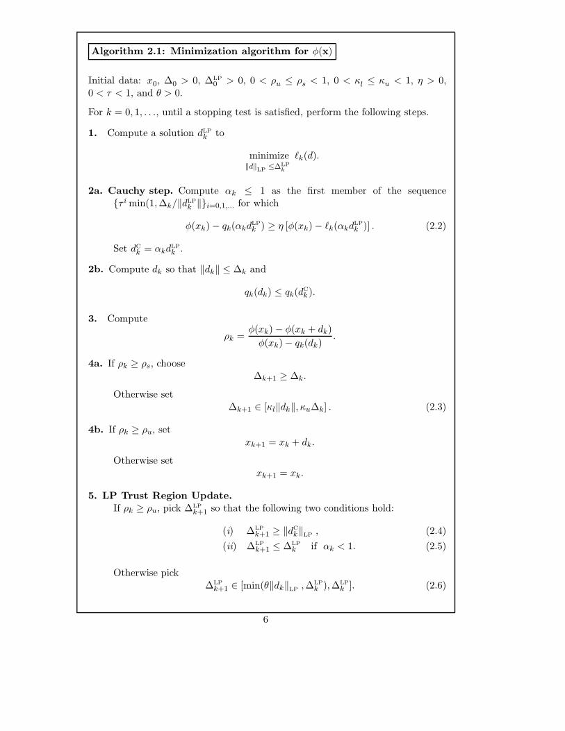
Algorithm 2.1: Minimization algorithm for φ(x)

Initial data: x0, ∆0 > 0, ∆LP

0 > 0, 0 < ρu ≤ ρs < 1, 0 < κl ≤ κu < 1, η > 0,0 < τ < 1, and θ > 0.

For k = 0, 1, . . ., until a stopping test is satisfied, perform the following steps.

1. Compute a solution dLP

k to

minimize‖d‖

LP≤∆LP

k

`k(d).

2a. Cauchy step. Compute αk ≤ 1 as the first member of the sequenceτ i min(1,∆k/‖dLP

k ‖i=0,1,... for which

φ(xk) − qk(αkdLP

k ) ≥ η [φ(xk) − `k(αkdLP

k )] . (2.2)

Set dC

k = αkdLP

k .

2b. Compute dk so that ‖dk‖ ≤ ∆k and

qk(dk) ≤ qk(dC

k ).

3. Compute

ρk =φ(xk) − φ(xk + dk)

φ(xk) − qk(dk).

4a. If ρk ≥ ρs, choose∆k+1 ≥ ∆k.

Otherwise set∆k+1 ∈ [κl‖dk‖, κu∆k] . (2.3)

4b. If ρk ≥ ρu, setxk+1 = xk + dk.

Otherwise setxk+1 = xk.

5. LP Trust Region Update.

If ρk ≥ ρu, pick ∆LP

k+1 so that the following two conditions hold:

(i) ∆LP

k+1 ≥ ‖dC

k‖LP, (2.4)

(ii) ∆LP

k+1 ≤ ∆LP

k if αk < 1. (2.5)

Otherwise pick∆LP

k+1 ∈ [min(θ‖dk‖LP,∆LP

k ),∆LP

k ]. (2.6)

6

Step 1 of Algorith 2.1 aims to find the largest reduction in the linearized model withinits trust region—we refer to this as the linearized problem, and attach the suffix LP toquantities associated with it. The intentions here are twofold.

Firstly, the aim is to identify constraints whose inclusion in the working set for anEQP results in progress in the overall minimization. Ideally near the solution these willcorrespond to active constraints at the solution. This is not the issue under considerationhere, but it does have some ramifications on the design of our algorithm since we hope thatour algorithm class is broad enough to permit correct identification of the active constraintset at the solution.

Secondly, the direction given by dLP

k is also used to define the Cauchy step dC

k , which, asin many trust region methods, is used to guarantee convergence to a critical point. This isbecause the value of the LP solution provides a measure of nearness to optimality, and theCauchy step is a step that provides corresponding improvement on the quadratic model.Condition (2.5) ensures that dC

k is short enough that the quadratic model value is relatedto the LP model. The descent properties of the Cauchy step are what drive the bulk ofour convergence theory; thus we ensure in Step 2b that the step actually taken, dk, sharesthese descent properties. Note that the Cauchy step dC

k satisfies the conditions of Step 2b,but the intention is to find a better step by solving a problem of the form (1.6).

Steps 3 and 4 are standard trust-region acceptance rules [4]. The ratio ρk of the actual tothe predicted reduction of φ is used as a step acceptance criterion. If this ratio is negative,or close to zero, the step is rejected and the overall trust-region radius reduced. Otherwisethe step will be accepted and, if ρk is close to one, the radius may be enlarged. We saythat iteration k is successful if ρk ≥ ρu. It is very successful if ρk ≥ ρs.

Step 5 gives the conditions imposed on the radius for the linear model. In [1] a specificstrategy is described that tries to relate ∆LP to the expected steplength so as to promoteselection of a good active set. However in this algorithm framework we only specify thecharacteristics such a strategy must have in order to guarantee global convergence. In thecase of a successful step, we impose a limit on how much ∆LP may be reduced, and allowincrease only if the full LP step was taken. If the step dk was not successful we allow forthe possibility of decreasing ∆LP as ∆k was decreased in Step 4a. 2

3 Convergence Results for a Fixed Penalty Function

In this section, we investigate the global convergence properties of Algorithm 2.1. In orderto proceed, we need to make the following assumptions on the problem and the algorithm:

P1. The functions f , g, and h in (1.1) are Lipschitz continuous and have Lipschitz contin-uous derivatives over a bounded convex set whose interior contains the closure of theiterates xk generated by Algorithm 2.1.

P2. The sequence of Hessian matrices Bk in (1.5) is bounded; thus there exists a constantβ > 0 such that |dT Bkd| ≤ β‖d‖2 for all k and all d ∈ IRn.

2The upper bound of one on αk in (2.5) is used for simplicity. However this bound can be generalized.

7

Assumption P2 is made to simplify the analysis; see [19] for an analysis of a compositenon-smooth optimization algorithm in which Bk is computed by quasi-Newton updating.(As pointed out in Section 1.1, both Algorithm 2.1 and the analysis in this section applyalso to the case where φ(x) = ω(F (x)), with `k and qk given by (1.10) and (1.11). In thiscase assumption P1 requires Lipschitz continuity of F, F ′ and ω.)

Under assumption P1 it follows immediately that φ(x) and `k(d) are Lipschitz contin-uous, and in particular that

|`k(d) − `k(0)| ≤ λ‖d‖LP

(3.1)

for some Lipschitz constant λ > 0.

The goal of our analysis is to prove that Algorithm 2.1 will find a critical point of φ.To do so, we follow Yuan [19] and define

Ψ(x,∆) = `(x, 0) − min‖d‖≤∆

`(x, d), (3.2)

which is the optimal decrease in the “linear” model `(x, d) for a radius of size ∆. We cancharacterize criticality of φ using Ψ.

Definition 3.1 x∗ ∈ IRn is a critical point (or stationary point) of φ if Ψ(x∗, 1) = 0.

For future reference we note that, from assumption P2 and the subsequent convexity of`(x, ·), we have in general

`(x, 0) − `(x, αd) ≥ α[`(x, 0) − `(x, d)], (3.3)

and more specifically,

φ(xk) − `k(αd) ≥ α[φ(xk) − `k(d)] (3.4)

for any α ∈ [0, 1].

We now establish a number of intermediate lemmas leading up to our main globalconvergence result. Our first result provides bounds on the achievable reduction in thelinearized model for a radius of size ∆ relative to that achieved with a radius of 1. Fromnow on we use the following notation.

Notation. The solution dLP of

min‖d‖

LP≤∆

`(x, d), (3.5)

will also be denoted as d∆ to emphasize its dependence on ∆. In particular d1 denotes thesolution of (3.5) when ∆ = 1.

Lemma 3.1 Suppose that assumptions P1 and P2 hold. Then

max(∆, 1)Ψ(xk, 1) ≥ Ψ(xk,∆) ≥ min(∆, 1)Ψ(xk, 1) (3.6)

for any scalar ∆ > 0.

8

Proof. Since d∆ is a solution of (3.5),

Ψ(xk,∆) = `(xk, 0) − `(xk, d∆).

There are two cases to consider. First consider the case ∆ ≤ 1. Since ‖d∆‖LP

≤ 1, thedefinition (3.2) implies that

Ψ(xk, 1) ≥ `(xk, 0) − `(xk, d∆) = Ψ(xk,∆),

which gives the left inequality of (3.6) in this case.To get the right inequality, we need to show that Ψ(xk,∆) ≥ ∆Ψ(xk, 1). By definition

of d∆ we have that ‖∆d1‖LP≤ ∆, and so by (3.2) and (3.3),

Ψ(xk,∆) ≥ `(xk, 0) − `(xk,∆d1)

≥ ∆(`(xk, 0) − `(xk, d1))

= ∆Ψ(xk, 1).

This gives us (3.6) when ∆ ≤ 1. In the case ∆ ≥ 1 we need to establish

∆Ψ(xk, 1) ≥ Ψ(xk,∆) ≥ Ψ(xk, 1),

but these inequalities follow immediately by making the above two-case argument with thevalues ∆ and 1 interchanged. 2

Lemma 3.1 essentially states that Ψ(x, ·) is concave and monotonically increasing.We shall also need the following result which states that, at a non-critical point of φ,

the trust-region bound for the linearized problem, ‖d∆‖LP

≤ ∆, is active whenever the

radius ∆ is small enough. For brevity, let Ψk(∆)def= Ψ(xk,∆).

Lemma 3.2 Suppose that assumptions P1–P2 hold (and thus that there is a Lipschitzconstant λ for which (3.1) holds) and that Ψk(1) 6= 0. Then if d∆ is a solution of (3.5)when x = xk,

‖d∆‖LP

≥ min(∆,Ψk(1)

λ). (3.7)

Proof. As before, let d1 denote a solution of (3.5) when x = xk and ∆ = 1. Supposethat ‖d∆‖

LP< Ψk(1)/λ. Then (3.1) gives that

`k(d∆) ≥ `k(0) − λ‖d∆‖LP

> `k(0) − Ψk(1) = `k(d1). (3.8)

If ∆ ≥ 1 this contradicts our definition of d∆ as a solution of (3.5), so we must have‖d∆‖

LP≥ Ψk(1)/λ and thus (3.7) in this case. If ∆ < 1 then (3.8) and the convexity of `k

imply that `k is strictly decreasing along a line from d∆ to d1 (at least initially). Therefore,since d∆ minimizes `k, it cannot lie in the strict interior of the trust region ‖d‖

LP≤ ∆,

and hence ‖d∆‖LP

= ∆. 2

The next result provides a lower bound on the achievable reduction in the piecewisequadratic model in terms of the stepsize, the trust-region radius for the linearized problemand our criticality measure. At this point, recall that we use dLP

k to refer to the solution ofthe linear subproblem (3.5) solved in Step 1 of Algorithm 2.1.

9

Lemma 3.3 Suppose that assumptions P1–P2 hold. Then the model decrease satisfies

φ(xk) − qk(dk) ≥ φ(xk) − qk(dC

k) ≥ ηαkΨk(∆LP

k ) ≥ ηαk min(∆LP

k , 1)Ψk(1).

Proof. The first inequality follows directly from the requirement in Step 2b of Algo-rithm 2.1. To prove the second, note that inequality (3.4) and the requirement in Step 2agive that

φ(xk) − qk(dC

k ) = φ(xk) − qk(αkdLP

k ) ≥ η [φ(xk) − `k(αkdLP

k )]≥ ηαk [φ(xk) − `k(d

LP

k )] = ηαkΨk(∆LP

k ).

The third inequality follows immediately from Lemma 3.1. 2

Next, we establish an intuitive bound on the error introduced when using our quadraticapproximation to φ.

Lemma 3.4 Suppose that assumptions P1 and P2 hold. Then

|qk(dk) − φ(xk + dk)| ≤ M‖dk‖2

for some positive constant M .

Proof. As pointed out in Section 1.1 the function φ can be expressed as φ(x) = ω(F (x))where F and ω are defined as in (1.8) and (1.9). It follows from assumption P1 that F hasa Lipschitz continuous derivative with constant λF, which implies that

‖F (xk + dk) − F (xk) − F ′(xk)dk‖ ≤ λF‖dk‖2.

Since the function ω is Lipschitz continuous with some constant λω, this inequality, togetherwith Assumption P2, implies that

|qk(dk) − φ(xk + dk)| = |ω(F (xk) + F ′(xk)dk) + 1

2dT

k Bkdk − ω(F (xk + dk))|

≤ λω‖F (xk + dk) − F (xk) − F ′(xk)dk‖ + 1

2β‖dk‖

2

≤ (λωλF + 1

2β)‖dk‖

2

= M‖dk‖2

where M = λωλF + 1

2β. 2

The following technical result essentially says that either the Cauchy step is on theboundary of one of our trust regions, or it has a lower bound proportional to the optimalitycriterion.

Lemma 3.5 Suppose that assumptions P1 and P2 hold. Then at any iteration of Algo-rithm 2.1

αk∆LP

k ≥ ‖dC

k‖LP≥ min

(

∆k

γ,∆LP

k ,Ψk(1)

λ,min

(

1,1

∆LP

k

)

2(1 − η)τΨk(1)

βγ2

)

. (3.9)

10

Proof. The first inequality in (3.9) follows immediately since

‖dC

k‖LP= αk‖d

LP

k ‖LP

≤ αk∆LP

k .

To establish the second inequality, suppose first that the decrease condition (2.2) in Step2a of Algorithm 2.1 is immediately satisfied for αk = min(1,∆k/‖dLP

k ‖). Then, using (2.1)and Lemma 3.2,

‖dC

k‖LP= ‖αkd

LP

k ‖LP

= min

(

∆k

‖dLP

k ‖, 1

)

‖dLP

k ‖LP

≥ min

(

∆k

γ,∆LP

k ,Ψk(1)

λ

)

, (3.10)

which gives the first three terms in (3.9). On the other hand if αk < min(1,∆k/‖dLP

k ‖),then the decrease condition (2.2) must have been violated for αk/τ , and so

φ(xk) − qk(αkdLP

k /τ) = φ(xk) − `k(αkdLP

k /τ) − 1

2(αk/τ)2(dLP

k )T BkdLP

k

≤ η [φ(xk) − `k(αkdLP

k /τ)] . (3.11)

Now using Assumption P2, (2.1), (3.4) and Lemma 3.1, this inequality implies that

1

2(αk/τ)2(dLP

k )T BkdLP

k ≥ (1 − η) [φ(xk) − `k(αkdLP

k /τ)]1

2(αk/τ)2βγ2‖dLP

k ‖2LP

≥ (1 − η)(αk/τ)Ψk(∆LP

k )1

2(αk/τ)βγ2‖dLP

k ‖LP

∆LP

k ≥ (1 − η)min(∆LP

k , 1)Ψk(1)

αk‖dLP

k ‖LP

≥2(1 − η)τ

βγ2min

(

1,1

∆LP

k

)

Ψk(1). (3.12)

Since αkdLP

k = dC

k , this inequality combined with (3.10) gives the second inequality in (3.9).2

Our next result is crucial. It provides lower bounds on both the trust-region radius ∆k

and the length of the Cauchy step at a non-critical iterate in the case where the trust-regionradius for the linearized problem stays bounded.

Lemma 3.6 Suppose Algorithm 2.1 is applied to the problem (1.2) and that assumptionsP1–P2 hold. Suppose that ∆LP

k is bounded above, and that Ψk(1) ≥ δ > 0, ∀ k. Thenthere exists a constant ∆min > 0 such that

∆k ≥ ∆min and αk∆LP

k ≥∆min

γ(3.13)

for all k.

Proof. By assumption, there exists ∆max ≥ 1 such that

∆LP

k ≤ ∆max for all k. (3.14)

11

This inequality, the assumption Ψk(1) ≥ δ and Lemma 3.5 imply

‖dC

k‖LP≥ min

(

∆k

γ,∆LP

k ,∆crit

)

, (3.15)

where

∆crit = min

(

1

λ,2(1 − η)τ

βγ2∆max

)

δ. (3.16)

If the iteration is successful (ρk ≥ ρu), the rule (2.4) for choosing ∆LP

k in Step 5 of thealgorithm ensures that ∆LP

k+1 ≥ ‖dC

k‖LPand therefore

∆LP

k+1 ≥ min

(

∆k

γ,∆LP

k ,∆crit

)

. (3.17)

Let us now consider the case when the iteration is unsuccessful. Using Lemma 3.3 andequation (3.15) we have that

φ(xk) − qk(dk) ≥ φ(xk) − qk(dC

k ) ≥ ηαk min (∆LP

k , 1) δ = ηαk∆LP

k min

(

1

∆LP

k

, 1

)

δ

≥ηδ

∆max

αk∆LP

k ≥ηδ

∆max

min

(

∆k

γ,∆LP

k ,∆crit

)

.

(3.18)From Lemma 3.4 and (3.18) we have that

1 − ρk ≤|φ(xk + dk) − qk(dk)|

φ(xk) − qk(dk)≤

M‖dk‖2∆max

ηδ min

(

∆k

γ,∆LP

k ,∆crit

) . (3.19)

This implies that ‖dk‖ and (1 − ρk) are related by the inequality

‖dk‖2 ≥

(1 − ρk)ηδ

M∆max

min

(

∆k

γ,∆LP

k ,∆crit

)

(3.20)

at each step. Now since the iteration is unsuccessful, ρk < ρu and 1 − ρk > 1 − ρu, which,using (2.1) and (3.20), implies

θ2‖dk‖2LP

≥θ2

γ2‖dk‖

2 ≥ θ2 (1 − ρu)ηδ

γ2M∆max

min

(

∆k

γ,∆LP

k ,∆crit

)

≥ min

(

∆k

γ,∆LP

k ,∆crit,(1 − ρu)ηθ2δ

γ2M∆max

)2

.

Using this fact and the lower bound in (2.6) we have that, if the step is unsuccessful

∆LP

k+1 ≥ min

(

∆k

γ,∆LP

k ,∆crit,(1 − ρu)ηθ2δ

γ2M∆max

)

. (3.21)

Since the right side of (3.21) is clearly less than or equal to the right side of (3.17), whichholds when the step is accepted, then (3.21) must hold at each iteration.

12

We can consider ∆k in a similar fashion. If ∆k was decreased because ρk < ρs then1 − ρk > 1 − ρs and (3.20) implies

κ2l

γ2‖dk‖

2 ≥(1 − ρs)ηκ2

l δ

γ2M∆max

min

(

∆k

γ,∆LP

k ,∆crit

)

≥ min

(

∆k

γ,∆LP

k ,∆crit,(1 − ρs)ηκ2

l δ

γ2M∆max

)2

.

Together with (2.3) this implies

∆k+1

γ≥ min

(

∆k

γ,∆LP

k ,∆crit,(1 − ρs)ηκ2

l δ

γ2M∆max

)

. (3.22)

Since ∆k is not reduced when ρk ≥ ρs, (3.22) must then hold at each iteration.Now we can combine the recursions (3.21) and (3.22) to yield

min

(

∆k+1

γ,∆LP

k+1

)

≥ min

(

∆k

γ,∆LP

k ,∆crit,(1 − ρs)ηκ2

l δ

γ2M∆max

,(1 − ρu)ηθ2δ

γ2M∆max

)

(3.23)

which holds at every iteration. Applying this recursion over the entire sequence impliesthat for all k

min

(

∆k

γ,∆LP

k

)

≥ min

(

∆0

γ,∆LP

0 ,∆crit,(1 − ρs)ηκ2

l δ

γ2M∆max

,(1 − ρu)ηθ2δ

γ2M∆max

)

≡ ∆low,

Thus we can conclude that ∆k ≥ ∆min ≡ γ∆low for all k. It then follows from (3.15) andthe fact that ∆low ≤ ∆crit that

αk∆LP

k ≥ ‖dC

k‖LP≥ ∆low =

∆min

γ

for all k. 2

This immediately enables us to deduce that if the algorithm is unable to make progress,it must be because it has reached a critical point.

Corollary 3.7 Suppose that assumptions P1 and P2 hold, and that there are only finitelynumber of iterations for which ρk ≥ ρu. Then xk = x∗ for all sufficiently large k, and x∗ isa critical point of φ(x).

Proof. Step 4 of the algorithm ensures that if there are only a finite number of (successful)iterations for which ρk ≥ ρu, then xk = x∗ for all k > k0 for some k0 ≥ 0. Moreover,Ψk(1) = Ψk0

(1) for all k ≥ k0. Furthermore, as ρk < ρu for all k ≥ k0, the update rulesfor the trust regions imply that ∆k converges to zero and ∆LP

k is bounded above for all k.But then Ψk(1) = 0 for all k ≥ k0, since otherwise Lemma 3.6 contradicts the fact that ∆k

converge to zero. It thus follows from Definition 3.1 that x∗ is a critical point of φ. 2

Finally we are able to state our main global convergence result.

13

Theorem 3.8 Suppose Algorithm 2.1 is applied to the problem (1.2) and that assumptionsP1–P2 hold. If the sequence φ(xk) is bounded below then either

Ψl(1) = 0 for some l ≥ 0

orlim infk→∞

Ψk(1) = 0.

Proof. If there are only a finite number of successful iterations, the first of the statedpossibilities follows immediately from Corollary 3.7. Otherwise, there is an infinite subse-quence K of successful iterations. This means that ρk ≥ ρu, and φ(xk) is bounded frombelow, for all k ∈ K.

The proof now proceeds by contradiction. Assume there is a constant δ such thatΨk(1) ≥ δ > 0, ∀ k ∈ K. We will consider separately the two cases, when the LP trust-region radius ∆LP

k is bounded above, and the case when ∆LP

k is unbounded.Case 1. If ∆LP

k is bounded above, it follows from Lemma 3.6 that ∆k ≥ ∆min > 0.For our infinite subsequence K of successful iterations, Lemmas 3.3 and 3.6 give

φ(xk) − φ(xk+1) ≥ ρu(φ(xk) − qk(dk))

≥ ρuηαk min(∆LP

k , 1)δ

≥ ρuηαk∆LP

k min(1, 1/∆LP

k )δ

≥ ρuη∆minδ/(γ∆max) > 0,

for all k ∈ K, where ∆max > 1 is the upper bound for ∆LP

k . But then summing this inequalityover all k ∈ K contradicts the fact that the sequence φ(xk) is bounded from below. ThusCase 1 does not occur.

Case 2. Suppose that the LP trust-region radius ∆LP

k is unbounded. Then, sincethe radius is only increased in Step 5 of Algorithm 2.1 when αk ≥ 1, there is an infinitesequence K such that ∆LP

k > 1, αk ≥ 1 and ρk ≥ ρu, for all k ∈ K. Then from Lemma 3.3we have

φ(xk) − φ(xk+1) ≥ ρu(φ(xk) − qk(dk))

≥ ρuηαk min(∆LP

k , 1)Ψk(1)

≥ ρuηΨk(1)

≥ ρuηδ,

for all k ∈ K. This again contradicts the assumption that φ(x) is bounded from below,and Case 2 cannot occur.

Cases 1 and 2 therefore imply that the assumption Ψk(1) ≥ δ > 0, ∀ k must be falsewhich proves the desired result

lim infk→∞

Ψk(1) = 0.

2

This result guarantees that, if φ(x) is bounded below, the criticality criterion Ψk(1) even-tually becomes arbitrarily small. This implies that if the sequence xk is bounded thereexists an accumulation point of Algorithm 2.1 which is a critical point for (1.2).

14

4 A Penalty Method for Nonlinear Programming

We now discuss how to automatically adjust the penalty parameter σ as our algorithmproceeds so as to encourage convergence to a critical point of (1.1). We will make use ofthe following definitions.

We letv(x) = ‖h(x)‖ + ‖g−(x)‖ (4.1)

be a measure of constraint violation, so that the penalty function (1.3) can be written as

φσ(x) = f(x) + σv(x). (4.2)

We define a (piecewise) linear model of the constraint violation by

`v(x, d) = ‖h(x) + ∇h(x)T d‖ + ‖(g(x) + ∇g(x)T d)−‖. (4.3)

We can therefore write the model (1.4) of the penalty function by

`φσ(x, d) = f(x) + ∇f(x)T d + σ`v(x, d). (4.4)

Since the penalty parameter σ will now vary, we write the measure of criticality (3.2) forthe penalty function as

Ψσ(x,∆) = `φσ(x, 0) − min‖d‖≤∆

`φσ(x, d). (4.5)

Definition 3.1 states that x∗ ∈ IRn is a critical point of the penalty function φσ if Ψσ(x∗, 1) =0. Criticality of the measure of constraint violation v(x) will be measured by the function

θ(x,∆) = `v(x, 0) − min‖d‖≤∆

`v(x, d). (4.6)

Definition 4.1 x∗ ∈ IRn is a critical point of the infeasibility measure v(x) if θ(x∗, 1) = 0.

It is well known [11] that the penalty function (4.2) is exact in the sense that, forsufficiently large values of σ, strict local minimizers of the nonlinear program (1.1) thatsatisfy the Mangasarian-Fromovitz constraint qualification (MFCQ) are minimizers of φσ.We are also interested in the converse result, given that our algorithm minimizes the penaltyfunction.

Theorem 4.1 If x∗ is a critical point of φσ for some σ, and is feasible for (1.1), then x∗

is a KKT point of the nonlinear program (1.1). If x∗ is infeasible and is a critical point ofφσ for all sufficiently large σ then x∗ is an infeasible critical point of v(x).

Proof. At a feasible critical point x∗ of φσ, the vector d = 0 minimizes `φσ(x∗, d) , whichimplies that d = 0 is an optimal feasible solution of the linear program

minimized

dT∇f(x∗)

subject to h(x∗) + ∇hi(x∗)T d = 0

g(x∗) + ∇gi(x∗)T d ≥ 0.

(4.7)

15

Since the constraints of (4.7) are linear, the KKT conditions for (4.7) are satisfied, and theKKT conditions for (4.7) are identical to the KKT conditions for (1.1).

Suppose that x∗ is infeasible and assume, by way of contradiction, that θ(x∗, 1) > 0.Then by (4.6), there exists ‖d∗‖ ≤ 1 such that `v(x∗, 0) − `v(x∗, d

∗) > 0, and therefore forany σ large enough

−∇f(x∗)T d∗ + σ (`v(x∗, 0) − `v(x∗, d

∗)) > 0

or

`φσ(x∗, 0) − `φσ(x∗, d∗) > 0.

By (4.4) this implies that Ψσ(x∗, 1) > 0 for arbitrarily large σ, contradicting the assumptionthat x∗ is a critical point for φσ, for all large σ. This contradiction implies that, if x∗ isinfeasible, then θ(x∗, 1) = 0. 2

4.1 Penalty Update Procedure

Our penalty parameter strategy is based on our belief that it is as important to try todecrease the violation v(x) as it is to aim for criticality of φσ(x). Since we cannot be surethat there is a (locally) feasible point for the constraints (1.1b)–(1.1c), we might insteadmeasure the quality of the current violation in terms of its criticality, θ(x,∆). Thus wecontend it is reasonable to ask that the current value of the penalty parameter σ alwayssatisfies

Ψσ(xk, 1) ≥ ξσθ(xk, 1),

for some predefined constant ξ ∈ (0, 1), and to increase the current value if this inequalityfails. Hence we cannot consider our iterate to be near a critical point for φσ(x) unless it isnear a critical point of v(x).

The use of the criticality measure Ψσ(xk, 1) requires the solution of a linear programwith radius 1. Since the algorithm computes the quantity Ψσ(xk,∆k) at every iteration, wewould instead prefer to use this quantity to estimate criticality, thereby avoiding the extracomputational cost of solving a second linear program. As we show below, this is possibleso long as ∆k lies within a preset interval [δmin, δmax]. If ∆k is not in this interval, we willuse Ψσ(xk, δk) to measure criticality, where δk is the closest value to ∆k in [δmin, δmax].

Based on this strategy, the set of permissible penalty parameters at an iterate xk, withtrust region radius ∆k, is defined as

Ω(xk, δk)def= σ | Ψσ(xk, δk) ≥ ξσθ(xk, δk) .

Of course, computation of the quantity θ(xk, δk) also involves the solution of an addi-tional linear program, but once xk is near the feasible region, linearized feasibility is likelyto be attainable inside the trust region so that θ(xk, δk) = v(xk), and the stronger buteasier-to-check condition, Ψσ(xk, δk) ≥ ξσv(xk), will often hold.

We now describe an algorithm for solving the nonlinear programming problem (1.1) inwhich the penalty parameter is updated at every iteration. It makes use of Algorithm 2.1to generate steps.

16

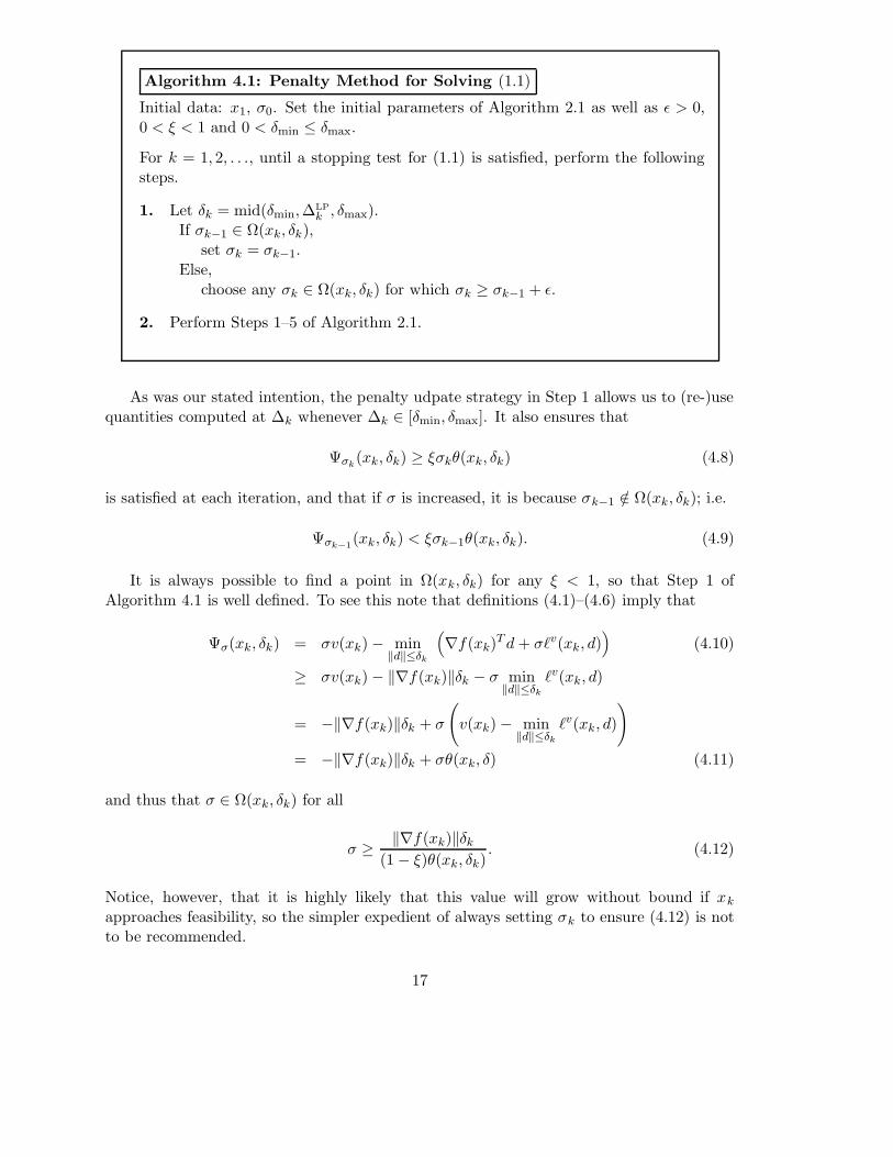
Algorithm 4.1: Penalty Method for Solving (1.1)

Initial data: x1, σ0. Set the initial parameters of Algorithm 2.1 as well as ε > 0,0 < ξ < 1 and 0 < δmin ≤ δmax.

For k = 1, 2, . . ., until a stopping test for (1.1) is satisfied, perform the followingsteps.

1. Let δk = mid(δmin,∆LP

k , δmax).If σk−1 ∈ Ω(xk, δk),

set σk = σk−1.Else,

choose any σk ∈ Ω(xk, δk) for which σk ≥ σk−1 + ε.

2. Perform Steps 1–5 of Algorithm 2.1.

As was our stated intention, the penalty udpate strategy in Step 1 allows us to (re-)usequantities computed at ∆k whenever ∆k ∈ [δmin, δmax]. It also ensures that

Ψσk(xk, δk) ≥ ξσkθ(xk, δk) (4.8)

is satisfied at each iteration, and that if σ is increased, it is because σk−1 /∈ Ω(xk, δk); i.e.

Ψσk−1(xk, δk) < ξσk−1θ(xk, δk). (4.9)

It is always possible to find a point in Ω(xk, δk) for any ξ < 1, so that Step 1 ofAlgorithm 4.1 is well defined. To see this note that definitions (4.1)–(4.6) imply that

Ψσ(xk, δk) = σv(xk) − min‖d‖≤δk

(

∇f(xk)T d + σ`v(xk, d)

)

(4.10)

≥ σv(xk) − ‖∇f(xk)‖δk − σ min‖d‖≤δk

`v(xk, d)

= −‖∇f(xk)‖δk + σ

(

v(xk) − min‖d‖≤δk

`v(xk, d)

)

= −‖∇f(xk)‖δk + σθ(xk, δ) (4.11)

and thus that σ ∈ Ω(xk, δk) for all

σ ≥‖∇f(xk)‖δk

(1 − ξ)θ(xk, δk). (4.12)

Notice, however, that it is highly likely that this value will grow without bound if xk

approaches feasibility, so the simpler expedient of always setting σk to ensure (4.12) is notto be recommended.

17

4.2 Penalty Method Analysis

We begin by recasting the inequality (4.8) in terms of Ψσ(xk, 1) instead of Ψσ(xk, δk).To do this we recall Lemma 3.1 and note that, since the function θ(x, δ), like Ψ(x, δ), ismonotonically increasing and concave in δ, the same arguments as used in the proof ofLemma 3.1 imply that

min(δk, 1)θ(xk, 1) ≤ θ(xk, δk) ≤ max(δk, 1)θ(xk, 1). (4.13)

This then implies the following bound.

Lemma 4.2 The values σk generated by Algorithm 4.1 satisfy

Ψσk(xk, 1) ≥ ξ min

(

δmin,1

δmax

)

σkθ(xk, 1). (4.14)

Proof. Using (3.6) followed by (4.8), followed by (4.13) yields:

Ψσk(xk, 1) ≥

Ψσk(xk, δk)

max(δk, 1)≥

ξσkθ(xk, δk)

max(δk, 1)≥ ξσk

min(δk, 1)

max(δk, 1)θ(xk, 1),

which gives (4.14), since δk ∈ [δmin, δmax]. 2

We now present two convergence results for Algorithm 4.1 that rely heavily on theconvergence properties of Algorithm 2.1. We first consider the case when the penaltyparameter is updated only a finite number of times.

Theorem 4.3 Suppose Algorithm 4.1 applied to problem (1.1) generates a bounded se-quence of iterates and that assumptions P1 and P2 hold. If σk is bounded, then there is acluster point x∗ of the sequence xk which is either a KKT point of the nonlinear program(1.1) or a critical point of v.

Proof. Since σk is bounded, it follows from Step 1 of Algorithm 4.1 that σk = σ isconstant for all large k. Algorithm 4.1 therefore reduces to Algorithm 2.1, i.e., to theminimization of a single penalty function. By Theorem 3.8, if φσk

(xk) is bounded below,there is a limit point x∗ of the sequence of iterates xk such that

Ψσ(x∗, 1) = 0. (4.15)

If x∗ is infeasible, since there is a subsequence xl with Ψσ(xl, 1) → 0 and since (4.14)holds at each iteration, we must have that θ(xl, 1) → 0. Then, since θ(·, 1) is continuous,θ(x∗, 1) = 0. Therefore x∗ is an infeasible critical point.

If x∗ is feasible, i.e. v(x∗) = 0, then it follows immediately from Theorem 4.1 that x∗ isa KKT point for the nonlinear program (1.1). 2

Our final result describes possible outcomes when the penalty parameter is unbounded.

Theorem 4.4 Suppose that Algorithm 4.1 generates a bounded sequence of iterates xkand that σk → ∞. Then either:

18

(i) the sequence xk is not asymptotically feasible (i.e. v(xk) 6→ 0), in which case thereis an infeasible cluster point x∗ that satisfies θ(x∗, 1) = 0; or

(ii) The sequence xk is feasible in the sense that v(xk) → 0. In this case, either: (a)there is a cluster point of xk that satisfies the KKT conditions; or (b) there is a feasiblecluster point of xk at which MFCQ is violated.

Proof. Consider the sequence of iterates at which the penalty parameter is increased. Foreach k in this subsequence, condition (4.9) holds, and thus we have

Ψσk−1(xk, δk) < ξσk−1θ(xk, δk).

Now (4.11) holds here, so

Ψσk−1(xk, δk) ≥ −‖∇f(xk)‖δk + σk−1θ(xk, δk)

and thus, using (4.13),

(1 − ξ)σk−1 ≤‖∇f(xk)‖δk

θ(xk, δk)≤

‖∇f(xk)‖δk

θ(xk, 1)min(1, δk))≤

‖∇f(xk)‖δmax

θ(xk, 1). (4.16)

But as σk, and consequently σk−1, is assumed unbounded and ∇f(xk) is bounded,it follows that, for that subsequence of xk for which σ was increased, we have θ(xk, 1) → 0.

If lim sup v(xk) > 0, then, since the sequence xk is bounded and θ(xk, 1) → 0, there isa limit point with v(x) > 0 and θ(x, 1) = 0, i.e., x is an infeasible stationary point of v(x).This implies (i) in that case.

On the other hand, if lim v(xk) = 0 then there is a cluster point x with v(x) = 0. If xsatisfies MFCQ, then ∇h(x) has full rank and there is a direction ‖dM‖ < δmin such that

∇h(x)T dM = 0 = −h(x) and ∇g(x)T dM + g(x) > 0.

Suppose by way of contradiction that x is not a KKT point. Then there is a first orderfeasible descent direction ‖dF ‖ < δmin such that

∇h(x)T dF = 0 = −h(x), ∇g(x)T dF + g(x) ≥ 0 and ∇f(x)T dF < 0.

Clearly there is a convex combination d = (1 − α)dF + αdM , with α ∈ (0, 1), such that

∇h(x)T d + h(x) = 0, (4.17)

∇g(x)T d + g(x) > 0 and ∇f(x)T d < 0.

Now since ∇h(x) has full rank, for any x sufficiently near x there is a unique vectord(x) of the form

d(x) = d + ∇h(x)u(x) (4.18)

for some u(x) ∈ Rm , which (non-uniquely) solves

h(x) + ∇h(x)T d(x) = 0. (4.19)

19

To see this note that (4.18)–(4.19) imply

[

h(x) + ∇h(x)T d]

+ ∇h(x)T∇h(x)u(x) = 0. (4.20)

Since h is smooth, this equation shows that u(x) is uniquely defined in a neighborhood ofx, and varies continuously with x—and so does d(x). Furthermore, by (4.17) the term insquare brackets in (4.20) can be made arbitrarily small if x is close to x, and hence d(x) isarbitrarily close to d.

Using these facts we have that d(x) satisfies

∇g(x)T d(x) + g(x) > 0 (4.21)

∇f(x)Td(x) < 0 (4.22)

for x sufficiently near x.Now note that since ‖d(x)‖ < δmin, we have by (4.3), (4.19) and (4.21) that

`v(x, d(x)) = 0. By the non-negativity of `v(x, d(x)) and the definition (4.6) this impliesthat θ(x) = `v(x, 0) = v(x). In addition, since ∇f(x)T d(x) < 0, we have from (4.10) that

Ψσ(x, δ) > σv(x) = σθ(x, δ)

for any δ ≥ δmin. Therefore, for any iterate xk sufficiently near x, σ ∈ Ω(xk, δk) for allσ ≥ 0. As a result, for this subsequence of iterates, σ is never updated in a neighborhoodof x.

This argument applies to any feasible limit point that satisfies MFCQ. Therefore itis not possible for all such points to have a descent direction, for otherwise the penaltyparameter would be updated only a finite number of times, contradicting the assumptionthat σk → ∞. In other words, we cannot have that all limit points satisfy MFCQ and arenot KKT points. This proves (ii). 2

Thus we are able to embed a relatively simple penalty-parameter update scheme withinAlgorithm 2.1 and derive useful convergence results. Another possibility which could betried is to update the penalty parameter as needed once a globally convergent method hasapproximately minimized φσ with the current (fixed) σ. Rules to achieve this are known[4, 12], but we are concerned that this may prove to be inefficient, particularly when aninappropriate initial σ is specified.

In the current version of the exact penalty method Slique [1], the penalty parameteris updated by a procedure that requires σk ∈ Ω(xk, δk) at each iteration, as well as somefurther conditions. Therefore Theorem 4.3 essentially holds for Slique. 3 However, becauseof the additional conditions on σk, it is not clear whether a result like Theorem 4.4 can beproved for Slique.

5 Conclusions and Perspectives

In this paper we have proposed a trust-region algorithm for nonlinear optimization thatuses a combination of linear and quadratic model steps and has separate quasi-autonomous

3This is true of the current implementation, but the description in [1] differs in some minor details.

20

trust-regions to control these. At least one subsequence generated by the algorithm is shownto be globally convergent to a critical point of the problem under modest assumptions. Ourframework for trust-region radius updates is deliberately general. This is because we wishedit to apply in the case of the current implementation of our evolving nonlinear programmingcode Slique [1] as well as to cover its future evolution.

We have not considered the ultimate convergence rate of the algorithm, nor its abilityto identify the optimal active constraints in a finite number of iterations (these two aspectsare most likely closely linked [9]), although we have strong numerical evidence to suggestthat the latter does occur and that the convergence rate may thereafter be made to besuperlinear. The study of these and other issues is ongoing.

Acknowledgment

The authors are grateful to two anonymous referees for their helpful comments on thispaper.

References

[1] R. H. Byrd, N. I. M. Gould, J. Nocedal, and R. A. Waltz. An active set algorithm fornonlinear programming using linear programming and equality constrained subprob-lems. Mathematical Programming, 100(1):27–48, 2004.

[2] C. M. Chin A new trust region based SLP-filter algorithm which uses EQP active-setstrategy. Ph. D. Thesis, Department of Mathematics, University of Dundee, Scotland,2001.

[3] C. M. Chin and R. Fletcher. On the global convergence of an SLP-filter algorithm thattakes EQP steps. Mathematical Programming, 96(1)161–177, 2003.

[4] A. R. Conn, N. I. M. Gould, and Ph. L. Toint. Trust-region methods. SIAM, Philadel-phia, 2000.

[5] A. R. Conn and T. Pietrzykowski. A penalty function method converging directly toa constrained optimum. SIAM Journal on Numerical Analysis, 14(2):348–375, 1977.

[6] R. Fletcher. Practical Methods of Optimization: Constrained Optimization, volume 2,chapter 14: Non-differentiable optimization. J. Wiley and Sons, Chicester and NewYork, 1981.

[7] R. Fletcher. A model algorithm for composite nondifferentiable optimization problems.Mathematical Programming Studies, 17:67–76, 1982.

[8] R. Fletcher and S. Leyffer, Nonlinear programming without a penalty function. Math-ematical Programming, 91(2):239–269, 2002.

[9] R. Fletcher and E. Sainz de la Maza. Nonlinear programming and non-smooth op-timization by successive linear programming. Mathematical Programming, 43(3):235–256, 1989.

21

[10] R. W. Gate. Development of algorithms for solving large optimization problems. Ph.D. Thesis, Department of Mathematics, University of Dundee, Scotland, 2004.

[11] S. P. Han and O. L. Mangasarian. Exact penalty functions in nonlinear programming.Mathematical Programming, 17(3), 251–269, 1979.

[12] D. Q. Mayne and E. Polak. Feasible directions algorithms for optimisation problemswith equality and inequality constraints. Mathematical Programming, 11(1), 67–80,1976.

[13] T. Pietrzykowski. An exact potential method for constrained maxima. SIAM Journalon Numerical Analysis, 6(2):299–304, 1969.

[14] M. J. D. Powell. General algorithms for discrete nonlinear approximation calculations.In C. K. Chui, L. L. Schumaker, and J. D. Ward, editors, Approximation Theory IV,pages 187–218, London, 1983. Academic Press.

[15] E. Sainz de la Maza. Nonlinear programming algorithms based on `1 linear program-ming and reduced Hessian approximation. Ph. D. Thesis, Department of MathematicalScience, University of Dundee, Scotland, 1987.

[16] R. A. Waltz. Algorithms for large-scale nonlinear optimization. Ph. D. Thesis, De-partment of Electrical and Computer Engineering, Northwestern University, Evanston,Illinois, USA, 2002.

[17] S. J. Wright. An inexact algorithm for composite nondifferentiable optimization. Math-ematical Programming, 44(2):221–234, 1989.

[18] Y. Yuan. An example of only linear convergence of trust region algorithms for non-smooth optimization. IMA Journal of Numerical Analysis, 4(3):327–335, 1984.

[19] Y. Yuan. Conditions for convergence of trust region algorithms for non-smooth opti-mization. Mathematical Programming, 31(2):220–228, 1985.

[20] Y. Yuan. On the superlinear convergence of a trust region algorithm for non-smoothoptimization. Mathematical Programming, 31(3):269–285, 1985.

[21] Y. Yuan. On the convergence of a new trust region algorithm. Numerische Mathematik,70(4):515–539, 1995.

22