On the Computational Representation of Classical Logical ... · Replace this ﬁle with prentcsmacro.styfor your meeting, or with entcsmacro.styfor your meeting. Both can be found

Replace this file withprentcsmacro.sty for your meeting,or with entcsmacro.sty for your meeting. Both can befound at theENTCS Macro Home Page.

On the Computational Representation of ClassicalLogical Connectives

Jayshan Raghunandan and Alexander J. Summers

Department of Computing, Imperial College London,180 Queen’s Gate, London SW7 2RH, UK

Abstract

Many programming calculi have been designed to have a Curry-Howard correspondence with a classical logic. We investi-gate the effect that different choices of logical connective have on such calculi, and the resulting computational content.We identify two connectives ‘if-and-only-if’ and ‘exclusive or’ whose computational content is not well known, and whosecut elimination rules are non-trivial to define. In the case of the former, we define a term calculus and show that thecomputational content of several other connectives can be simulated. We show this is possible even for connectives notlogically expressible with ‘if-and-only-if’.

1 Introduction

There are many programming calculi which have been designedto have a Curry-Howardcorrespondence with a logical proof system. In recent yearssuch calculi have been designedto explore the computational content of Classical Logic (e.g. [2,4,6,8,11,12,14]). Differ-ent authors have chosen different sets of logical connectives to treat as primitive in theirlogic, and designed the syntax and reduction rules of their calculi accordingly. Implicationis the most popular choice of connective, since it is well-understood that its computationalbehaviour is related to function abstraction and application. There are calculi which donot use implication, for example that of Wadler [14]. Calculi exist which employ conjunc-tion, disjunction, negation, and even more esoteric connectives such as difference [1,2] andconstants for truth and falsity.

We consider logics with different primitive connectives and discuss general approachesto the design of corresponding term calculi. We restrict ourattention topropositionallog-ical connectives; an investigation of various approaches to employing quantifiers has beenstudied in [10].

We work in the logical context of the sequent calculus, a brief introduction to which isgiven in Section2. The style of our term calculi is based on that of theX -calculus [12],

1 Email: [email protected], [email protected]

c©2007 Published by Elsevier Science B. V.

http://www.math.tulane.edu/~entcs

mailto:[email protected]

mailto:[email protected]

Raghunandan & Summers

which has a Curry-Howard correspondence with a classical sequent calculus for implica-tion. TheX -calculus is presented in Section3. In Section4, we generalise the design ofX to that of analogous term calculi based on sequent calculi with different logical connec-tives. Section5 identifies a class of logical connectives to investigate, and for each, showshow to derive suitable term representations and associatedreduction rules. We identify thatthe computational content of the ‘if-and-only-if’ (↔) and ‘exclusive or’ (⊗) connectivesare not well understood. Section6 is a study of the ‘if-and-only-if’ connective, whose re-duction rules turn out to be non-trivial to define. We define a term calculus based only onthis connective, which we callX↔, and investigate its computational expressivity. As asurprising result we show that this new calculus can, given certain restrictions, simulate thereductions of several well-known logical connectives which are not themselves logicallyexpressible in terms of↔. As an example, we give an interpretation of theX -calculus intoX↔.

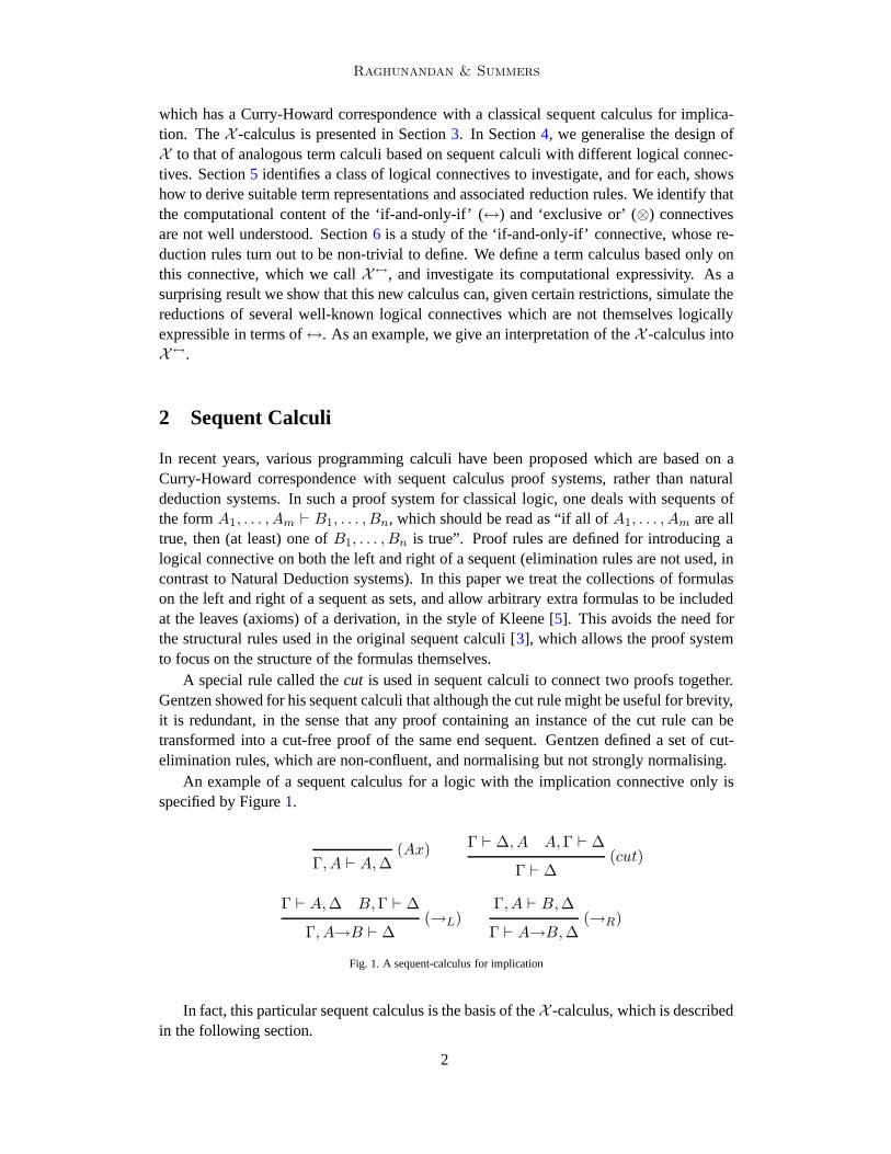
2 Sequent Calculi

In recent years, various programming calculi have been proposed which are based on aCurry-Howard correspondence with sequent calculus proof systems, rather than naturaldeduction systems. In such a proof system for classical logic, one deals with sequents ofthe formA1, . . . , Am ⊢ B1, . . . , Bn, which should be read as “if all ofA1, . . . , Am are alltrue, then (at least) one ofB1, . . . , Bn is true”. Proof rules are defined for introducing alogical connective on both the left and right of a sequent (elimination rules are not used, incontrast to Natural Deduction systems). In this paper we treat the collections of formulason the left and right of a sequent as sets, and allow arbitraryextra formulas to be includedat the leaves (axioms) of a derivation, in the style of Kleene[5]. This avoids the need forthe structural rules used in the original sequent calculi [3], which allows the proof systemto focus on the structure of the formulas themselves.

A special rule called thecut is used in sequent calculi to connect two proofs together.Gentzen showed for his sequent calculi that although the cutrule might be useful for brevity,it is redundant, in the sense that any proof containing an instance of the cut rule can betransformed into a cut-free proof of the same end sequent. Gentzen defined a set of cut-elimination rules, which are non-confluent, and normalising but not strongly normalising.

An example of a sequent calculus for a logic with the implication connective only isspecified by Figure1.

(Ax)Γ, A ⊢ A,∆

Γ ⊢ ∆, A A,Γ ⊢ ∆(cut)

Γ ⊢ ∆

Γ ⊢ A,∆ B,Γ ⊢ ∆(→L)

Γ, A→B ⊢ ∆

Γ, A ⊢ B,∆(→R)

Γ ⊢ A→B,∆

Fig. 1. A sequent-calculus for implication

In fact, this particular sequent calculus is the basis of theX -calculus, which is describedin the following section.

2


3 TheX -Calculus

Our work is based on theX -calculus [12]; an untyped term annotation for classical im-plicative sequent calculus. We recall here the basic definitions.

Definition 3.1 [X -Terms] The terms of theX -calculus are defined by the following syntax,wherex, y range over the infinite set ofsocketsandα, β over the infinite set ofplugs(sockets and plugs together form the set ofconnectors).

P,Q ::= 〈x.α〉 | yP β ·α | P β [y] xQ | Pα † xQ | Pα † xQ | Pα † xQ

capsule export mediator cut left-cut right-cut

The · symbolises that the connector underneath is bound in the attached subterm—abound socket is written as a prefix to the term, whereas a boundplug is written as a suffix.For example in the mediatorP β [y] xQ, occurrences ofβ are bound in the subtermP andoccurrences ofx are bound inQ. A connector which does not occur under a binder is saidto be free. We will usefp(P ) to denote the free plugs ofP , and similarlyfs(P ) for freesockets. We work moduloα-conversion (issues regardingα-conversion have been studiedin [13]). The reduction rules are specified below.

Definition 3.2 [Logical Rules] The logical rules are presented by:

(cap) : 〈y.α〉α † x〈x.β〉 → 〈y.β〉

(exp) : (yP β ·α)α † x〈x.γ〉 → yP β ·γ α 6∈ fp(P )

(med) : 〈y.α〉α † x(P β [x] zQ) → P β [y] zQ x 6∈ fs(P,Q)

(exp-med) : (yP β ·α)α † x(Qγ [x] zR) →

Qγ † y(P β † zR)

(Qγ † yP )β † zR

α 6∈ fp(P ),

x 6∈ fs(Q,R)

The first three logical rules above specify a renaming (reconnecting) pro cedure, whereasthe last rule specifies the basic computational step: it allows the body of the function fromthe export to be inserted between the two subterms of the mediator (the resulting cuts maybe bracketed either way, as shown).

Definition 3.3 [Activation Rules] We define twocut-activationrules.

(act-L) : Pα † xQ → Pα † xQ if P does not introduceα

(act-R) : Pα † xQ → Pα † xQ if Q does not introducex

where:P introducesx: EitherP = Qβ [x] yR andx 6∈ fs(Q,R), orP = 〈x.α〉

P introducesα: EitherP = xQβ ·α andα 6∈ fp(Q), orP = 〈x.α〉

An activated cut is processed by ‘pushing’ it systematically through the syntactic struc-ture of the circuit in the direction indicated by the tiltingof the dagger. Whenever an activecut meets a circuit exhibiting the connector it is trying to communicate with, a new (inac-tive) cut is ‘deposited’, representing an attempt to communicate at this level. The pushingof the active cut continues until the level of capsules is reached, where it is either deacti-vated or destroyed. Once again, the inactive cut can reduce via a logical rule, or pushing can

3


continue in the other direction. This behaviour is expressed by the following propagationrules.

Definition 3.4 [Propagation Rules]Left Propagation:

(† †) : 〈y.α〉α † xP → 〈y.α〉α † xP

(† cap) : 〈y.β〉α † xP → 〈y.β〉 β 6= α

(† exp-outs) : (yQβ ·α)α † xP → (y(Qα † xP )β ·γ)γ † xP , γ fresh

(† exp-ins) : (yQβ ·γ)α † xP → y(Qα † xP )β ·γ, γ 6= α

(† med) : (Qβ [z] yR)α † xP → (Qα † xP )β [z] y(Rα † xP )

(† cut-cap) : (Qβ † y〈y.α〉)α † xP → (Qα † xP )β † xP

(† cut) : (Qβ † yR)α † xP → (Qα † xP )β † y(Rα † xP ), R 6= 〈y.α〉

Right Propagation:

( ††) : Pα † x〈x.β〉 → Pα † x〈x.β〉

( †cap) : Pα † x〈y.β〉 → 〈y.β〉, y 6= x

( †exp) : Pα † x(yQβ ·γ) → y(Pα † xQ)β ·γ

( †med-outs) : Pα † x(Qβ [x] yR) → Pα † z((Pα † xQ)β [z] y(Pα † xR)),

z fresh

( †med-ins) : Pα † x(Qβ [z] yR) → (Pα † xQ)β [z] y(Pα † xR), z 6= x

( †cut-cap) : Pα † x(〈x.β〉β † yR) → Pα † y(Pα † xR)

( †cut) : Pα † x(Qβ † yR) → (Pα † xQ)β † y(Pα † xR), Q 6= 〈x.β〉

We write→ for the reduction relation generated by the logical, propagation and activa-tion rules. The following are admissible rules (see [12,13]).

Lemma 3.5 (Garbage Collection and Renaming)

(gc-L) : Pα † xQ → P, if α 6∈ fp(P )

(gc-R) : Pα † xQ → Q, if x 6∈ fs(Q)

(ren-L) : P δ † z〈z.α〉, → P [α/δ]

(ren-R) : 〈z.α〉α † xP , → P [z/x]

4 The Computational Representation of a Connective

In this section, we outline some of the techniques used in therest of the paper for derivingsuitable proof rules, corresponding syntax representations and reduction rules to representthe inclusion of a particular logical connective.

We useA,B, . . . as propositional variables and¬ to represent logical negation, whichbinds tighter than any other connective. We use◦ and• to represent arbitrary binary con-nectives (logical connectives which take two arguments). For formulasF1 andF2 we write

4


F1≡F2 (and say the formulas arelogically equivalent) if for all assignments of truth valuesto propositional variables,F1 andF2 have the same truth value as each other.

4.1 Sequent Rules

We will assume the rules for the axiom (c.f. capsule inX ) and the cut are present andunchanged in all the systems we discuss (see Figure1). For each logical connective ofinterest, suitable proof rules must be provided (or derived) for introducing the connectiveon the left and right-hand sides of a sequent (c.f.→L and→R of Figure1).

One important point is that for various logical connectivesone has a choice of howmany proof rules to incorporate. This is most easily seen in the different treatments ofpairing, typically relating to the∧ connective (although this notion is generalised in Section5). A term is usually provided to construct a pair, but there are different approaches to theproblem of dealing with pairs (making use of their individual components). One approachis to provide twoprojections, which reduce a pair to one or other of its component elements.Another is sometimes termed a ‘pattern-matching’ approach, in which both componentsare substituted in to some receiving term. These two approaches can be shown to be inter-derivable in our framework, and the decision of which to use is largely a matter of taste. Asan example, for the∧ connective (conjunction), the left introduction could be specified ineither of the following two ways:

Γ, A,B ⊢ ∆(∧L)

Γ, A ∧B ⊢ ∆or

{Γ, A ⊢ ∆

(∧L1)Γ, (A ∧B) ⊢ ∆

andΓ, B ⊢ ∆

(∧L2)Γ, (A ∧B) ⊢ ∆

}

In this paper we choose the ‘pattern-matching’ style; that is, we will always choose tohave exactly one left and right introduction rule for a binary connective.

It may not always be the case that a set of suitable sequent proof rules for a particularconnective are obvious. In this case, one can proceed as follows. To derive suitable sequentrules for a binary connective◦, say, choose a formulaF such thatF≡A◦B andF usesconnectives for which one already knows suitable proof rules. Now, try to construct whata ‘general’ sequent derivation which introduces this formula on the left and right of thesequent might be. Once all of the connectives inF have been introduced, it will not bepossible to proceed further in the derivation. All remaining sub-derivations to be completedtranslate to sub-proofs in the derived rule, while the formula F is replaced byA◦B for theend sequent. This process will give suitable proof rules forthe connective◦. This techniquewill be further illustrated and exploited in Sections5 and6.

4.2 Term Syntax

We work in the style of theX -calculus, since this gives a simple and symmetric treatmentof the inputs and outputs present within the syntax. When deriving the syntax to representa particular proof rule, formulas which occur on the left of asequent will become inputs(sockets)x, y, z, . . . while formulas on the right will be outputs (plugs)α, β, γ, . . .. Anysubproofs present in the rule will be represented as subterms of the syntax. Formulas whichdisappear from such subproofs by application of the proof rule (formulas which areboundby the rule) will correspond to bound connectors on the subterms, while a new formulawhich is introduced by the rule corresponds to a free connector of the appropriate kind.

With these ideas in mind, it should be clear to see that the term representation of the

5


sequent calculus in Figure1 could well be chosen to be the syntax ofX (see Definition3.1). For example, the→R rule has one subproof, which corresponds to a sub-termP ,say. It binds two formulas in this subproof, one on the left ofthe sequent and one on theright, therefore a socket and a plug ofP should be bound (sayx andα respectively). Therule introduces a new formula on the right of the sequent, which leads to a free plug beingpresent in the term representation (sayβ). One can easily see that theexport of theX -calculus, writtenxPα·β is such a representation, with the· being inactive syntax, designedto make the terms easier to parse.

As a further example, consider the→L rule. This has two subproofs, which becomesubtermsP andQ. Each has a single formula bound, on the right and left of the sequentsrespectively. Thus a plugα is bound inP and a sockety is bound inQ. Finally, a freesocketx should be introduced. The notationPα [x] yQ is chosen, with thex occurringbetween the two terms simply to provide a better intuition for how this term behaves; it actsas a ‘hole’ between the two subterms, into which a further term can be inserted to ‘mediate’betweenP andQ (this behaviour is seen in theexp-medrule).

4.3 Reduction Rules

Whichever logical connectives are employed, we will alwayskeep the followingX reduc-tion rules (which deal with cuts and capsules) in place:

cap,act-L,act-R, † †, † cap, † cut-cap, † cut, ††, †cap, †cut-cap, †cut

The notion of a plug or socket beingintroducedcan be generalised to sayP introducesx (respectively,α) iff x is free inP but not in any of its proper subterms.

Propagation rules must be defined for propagating left and right cuts through each syn-tactic construct. If a new syntax construct corresponds to aleft-introduction rule (i.e. itsfree connector is a socket), two rules must be given for propagating a right-cut over it (de-pending on whether the free connector is that which the cut isattempting to connect to), andone for propagating a left-cut (c.f.†med-outs, †med-ins, † med). The general approach isto push copies of the cut into the subterms, leaving a copy on the outside if an occurrence ofthe desired connector was present at this level (c.f.†med-outs). The appropriate rules forpropagation over a construct which introduces a plug may be derived symmetrically (twofor left cuts, one for right cuts).

This leaves the appropriate extra logical reduction rules to be defined. Each new syn-tax construct warrants a logical rule to specify a renaming of its introduced connector, viaa cut with a capsule (see the rulesexpandmed, for example). Finally, for each logicalconnective employed, a logical rule must be defined to show how a cut between the rightand left introduction of the connective may be reduced (c.f.the ruleexp-med). We callthis theprincipal logical rule for the connective, since it is the rule which specifies howthese structures may be removed from a proof, creating new cuts between their subtermsand simplifying the task of cut-elimination. The principalrule is the only one which can-not be methodically derived independent of the particular connective concerned. For thisreason, when investigating the representation of a particular connective, as far as reductionrules are concerned we will only concern ourselves with the principal logical rule for theconnective.

6


5 Comparing Logical Connectives

In this section, we compare various logical connectives, focusing on relationships betweenthem and how this affects their inclusion in a term calculus.For each connective we areinterested in the following three questions:

(i) What is a suitable term representation of its proof rules?

(ii) What is its principal reduction rule?

(iii) What computational content is gained by its inclusion?

5.1 Enumerating the connectives

There are an infinite number of possible logical connectives, since a connective may applyto an arbitrary (but usually fixed) number of arguments (hereon itsarity). It is extremelyrare in practice for authors to employ connectives with arity greater than two (althoughfor an example, see [7]). To decide on a set of connectives for our study, we found thefollowing three questions of interest:

(a) How many logical connectives are there of arityn (n ≥ 0)?

(b) How many of these depend on alln inputs (we say these havetrue arityn)?

(c) How many of thesealwaysdepend on alln inputs?

To explain the second question, take for example the binary connective which has inputsA andB and always evaluates toA (ignoringB). In a sense one could see this as a unaryconnective, since it only makes use of one input. This gives away of identifying thoseconnectives of arityn which we regard as degenerate cases.

The third question regards a stronger notion; that the valueof a connective should,in every input state, depend on all of its inputs. As a non-example, the evaluation of aconjunction (∧) may be ‘short-cut’; if its first argument turns out to be false then the secondneed not be considered. Thus conjunction does not satisfy the criterion outlined in the thirdquestion.

The answer to each of these questions is given by the following result:

Theorem 5.1 (Enumerating Logical Connectives)For any integern ≥ 0:

(a) There are22n

logical connectives of arityn.

(b) The number of these which depend on alln inputs (those of true arityn), t(n) is given

by the following formula:t(n) = 22n

−n−1∑

i=0

(n

i

)t(i).

(c) There are exactly two connectives of arityn which always depend on alln inputs;these are the parity function (which is true exactly when an even number of its argu-ments are), and its negation.

Proof.

(a) Each connective is exactly specified by a ‘truth-table’;defining whether it evaluatesto true or false in each of the2n possible input states. The result follows by countingall such truth tables.

(b) By counting; start with all connectives of arityn, and subtract off those which depend

7


on strictly fewer inputs. Since each of these may depend on a different subset of theactual inputs available, one must count them for each appropriate subset (hence the(ni

)).

(c) Let f be some such connective of arityn, which we represent as a function ofninputs,f(i1, i2, . . . , in). We write0 for a false input,1 for true, andi for the nega-tion on these inputs (i.e.1 = 0 etc.). Our condition onf states that given a set ofinput valuesi1, . . . , in, the value off(i1, i2, . . . , in) depends on all ofi1, . . . , in, orequivalently, if we change (negate) any one of the inputs, the value off(i1, i2, . . . , in)

must change. Now consider setting all inputs to0, and sayf(0, . . . , 0) = a wherea = 0 or a = 1. By our condition onf , if we now negate any one of the inputs, thevalue off(i1, i2, . . . , in) must bea. In general, letj be the number of true inputs, i.e.j = | {ik | 1 ≤ k ≤ n andik = 1} |. A straightforward induction onj shows that:

f(i1, i2, . . . , in) =

a if j is even

a if j is odd

Thusf is exactly specified by the choice ofa. Therefore there are exactly two suchfunctions, the parity function and its negation.

2

Examining the second part of this result, we see thatt(0) = 2. These two connectivesare the logical constants⊤ and⊥, which can be seen as connectives of arity0 (they can beseen as the parity and not-parity connectives of arity0). It is easy to see thatt(1) = 2 also,and these are the identity connective (which returns whatever input it receives unchanged)and negation (¬). Furthermore, we seet(2) = 10, i.e. there are 10 different logical con-nectives of true arity 2. These connectives are listed in thenext section, although the readermight find it interesting to try to name them all first!

We will henceforth only interest ourselves in connectives of arity 2 (and below). Ascommented, this choice is common in the literature. On a practical note, since the readermay verify thatt(3) = 218, an exhaustive analysis of all possible connectives of any greaterarity would be too cumbersome.

5.2 The Binary Connectives

In this section, we will give the complete set of possible binary connectives, and provide ananalysis of them with respect to the three questions outlined at the start of Section5. We areinterested in possible relationships between these connectives, and how these are reflectedby their computational counterparts. For example,duality is a well-known concept relatingbinary logical connectives, and it will be seen that this relationship carries over into theircomputational behaviour (this is related to the results of [2,14]).

We make use of the following relationships between connectives:

Definition 5.2 [Relating connectives] For any two binary connectives◦,•:

Duality We say• is thedual of ◦ iff A •B ≡ ¬(¬A ◦ ¬B).

Negation We say• is thenegationof ◦ iff A •B ≡ ¬(A ◦B).

Reversal We say• is thereverseof ◦ iff A •B ≡ B ◦A.

8


A∧B A∨B B−A A→B

A↑B A↓B B→A A−B

⊤ A B A↔B

⊥ ¬A ¬B A⊗B

D

D

N N

S S

S S

D

D

N NSS

S

S

N N

D D

D D

N D

S

S

N D

S

S

Note: ↑ = nand,↓ = nor,⊗ = xor

Fig. 2. Binary Connectives

Γ ⊢ B,∆ Γ, A ⊢ ∆(←L)

Γ, A←B ⊢ ∆

Γ, B ⊢ A,∆(←R)

Γ ⊢ A←B,∆

Fig. 3. Sequent Rules for reverse implication←

Flipping inputs We say• is obtained from◦ by flipping an inputif eitherA•B ≡ ¬A◦BorA •B ≡ A ◦ ¬B.

In all but the last case, these concepts describe self-inverse functions (e.g. the dual of thedual of a connective is the connective itself).

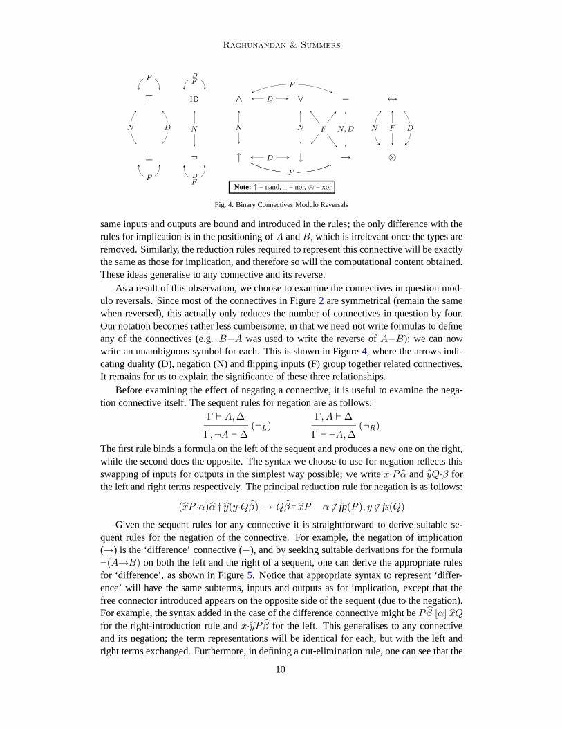
The binary connectives include conjunction (∧), disjunction (∨), nand (↑) and nor (↓).There is implication (→) and its reverse (←), and the so-called ‘difference’ operator (−),whereA−B ≡ A∧¬B. For the reverse connective of− (for which there is no standardsymbol) we tend to simply use− and swap the arguments, but will shortly be able todispense with this slight abuse of notation. As well as these, there is ‘if-and-only-if’ (↔),‘exclusive or’ (⊗), and the degenerate cases (⊤,⊥ and the identity and negation on eachargument, which we will writeID A,¬A, ID B and¬B). Although we call these degeneratecasesbinary connectives, we will treat them as having their true arities(e.g. when usingnegation we only mention the input which it uses). All these connectives are illustratedin Figure2, along with arrows to represent duality (D), negation (N) and reversal (R) ofconnectives.

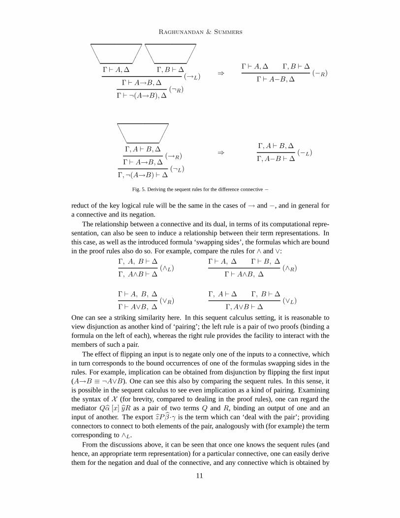
Firstly, we wish to examine the effect of the ‘reversal’ of a connective with respect to ourquestions of interest. For example, consider the connective←. A sensible pair of sequentrules for this connective is shown in Figure3. Deriving the syntax needed to represent theserules, we find that we can use exactly the same as that for implication. This is because the

9


⊤ ID ∧ ∨ − ↔

⊥ ¬ ↑ ↓ → ⊗

D

D

N N N, DFF

F

FF

N

D

F

D

F

N D

F

F

FN D

Note: ↑ = nand,↓ = nor,⊗ = xor

Fig. 4. Binary Connectives Modulo Reversals

same inputs and outputs are bound and introduced in the rules; the only difference with therules for implication is in the positioning ofA andB, which is irrelevant once the types areremoved. Similarly, the reduction rules required to represent this connective will be exactlythe same as those for implication, and therefore so will the computational content obtained.These ideas generalise to any connective and its reverse.

As a result of this observation, we choose to examine the connectives in question mod-ulo reversals. Since most of the connectives in Figure2 are symmetrical (remain the samewhen reversed), this actually only reduces the number of connectives in question by four.Our notation becomes rather less cumbersome, in that we neednot write formulas to defineany of the connectives (e.g.B−A was used to write the reverse ofA−B); we can nowwrite an unambiguous symbol for each. This is shown in Figure4, where the arrows indi-cating duality (D), negation (N) and flipping inputs (F) group together related connectives.It remains for us to explain the significance of these three relationships.

Before examining the effect of negating a connective, it is useful to examine the nega-tion connective itself. The sequent rules for negation are as follows:

Γ ⊢ A,∆(¬L)

Γ,¬A ⊢∆

Γ, A ⊢ ∆(¬R)

Γ ⊢ ¬A,∆

The first rule binds a formula on the left of the sequent and produces a new one on the right,while the second does the opposite. The syntax we choose to use for negation reflects thisswapping of inputs for outputs in the simplest way possible;we writex·Pα andyQ·β forthe left and right terms respectively. The principal reduction rule for negation is as follows:

(xP ·α)α † y(y·Qβ) → Qβ † xP α 6∈ fp(P ), y 6∈ fs(Q)

Given the sequent rules for any connective it is straightforward to derive suitable se-quent rules for the negation of the connective. For example,the negation of implication(→) is the ‘difference’ connective (−), and by seeking suitable derivations for the formula¬(A→B) on both the left and the right of a sequent, one can derive the appropriate rulesfor ‘difference’, as shown in Figure5. Notice that appropriate syntax to represent ‘differ-ence’ will have the same subterms, inputs and outputs as for implication, except that thefree connector introduced appears on the opposite side of the sequent (due to the negation).For example, the syntax added in the case of the difference connective might beP β [α] xQ

for the right-introduction rule andx·yP β for the left. This generalises to any connectiveand its negation; the term representations will be identical for each, but with the left andright terms exchanged. Furthermore, in defining a cut-elimination rule, one can see that the

10


AAA

��

�Γ ⊢ A,∆

AAA

��

�Γ, B ⊢∆

(→L)Γ ⊢ A→B,∆

(¬R)Γ ⊢ ¬(A→B),∆

⇒Γ ⊢ A,∆ Γ, B ⊢∆

(−R)Γ ⊢ A−B,∆

AAA

��

�Γ, A ⊢ B,∆

(→R)Γ ⊢ A→B,∆

(¬L)Γ,¬(A→B) ⊢∆

⇒Γ, A ⊢ B,∆

(−L)Γ, A−B ⊢∆

Fig. 5. Deriving the sequent rules for the difference connective −

reduct of the key logical rule will be the same in the cases of→ and−, and in general fora connective and its negation.

The relationship between a connective and its dual, in termsof its computational repre-sentation, can also be seen to induce a relationship betweentheir term representations. Inthis case, as well as the introduced formula ‘swapping sides’, the formulas which are boundin the proof rules also do so. For example, compare the rules for ∧ and∨:

Γ, A, B ⊢∆(∧L)

Γ, A∧B ⊢ ∆

Γ ⊢ A, ∆ Γ ⊢ B, ∆(∧R)

Γ ⊢ A∧B, ∆

Γ ⊢ A, B, ∆(∨R)

Γ ⊢ A∨B, ∆

Γ, A ⊢∆ Γ, B ⊢∆(∨L)

Γ, A∨B ⊢∆

One can see a striking similarity here. In this sequent calculus setting, it is reasonable toview disjunction as another kind of ‘pairing’; the left ruleis a pair of two proofs (binding aformula on the left of each), whereas the right rule providesthe facility to interact with themembers of such a pair.

The effect of flipping an input is to negate only one of the inputs to a connective, whichin turn corresponds to the bound occurrences of one of the formulas swapping sides in therules. For example, implication can be obtained from disjunction by flipping the first input(A→B ≡ ¬A∨B). One can see this also by comparing the sequent rules. In this sense, itis possible in the sequent calculus to see even implication as a kind of pairing. Examiningthe syntax ofX (for brevity, compared to dealing in the proof rules), one can regard themediatorQα [x] yR as a pair of two termsQ andR, binding an output of one and aninput of another. The exportzP β ·γ is the term which can ‘deal with the pair’; providingconnectors to connect to both elements of the pair, analogously with (for example) the termcorresponding to∧L.

From the discussions above, it can be seen that once one knowsthe sequent rules (andhence, an appropriate term representation) for a particular connective, one can easily derivethem for the negation and dual of the connective, and any connective which is obtained by

11


flipping an input. In particular, the six connectives which are joined to each other by variousarrows in Figure4 (including∧,∨ and→) all have related sequent rules. Each can in fact beregarded as a kind of pairing connective; the differences lie in whether inputs or outputs arebound in the two subterms which make up the pair, and whether the pair is made availableon an introduced input or output. We will sometimes refer to these six connectives as thepairing connectives.

As can be seen from Figure4, the remaining connectives come in related groups oftwo. The syntax and main rule for the negation connective have already been discussed,while the identity connective can be seen to have a very trivial computational content (atbest it provides a kind ofaliasing, where a connector is bound within a subterm and thenimmediately exported again with a new name).

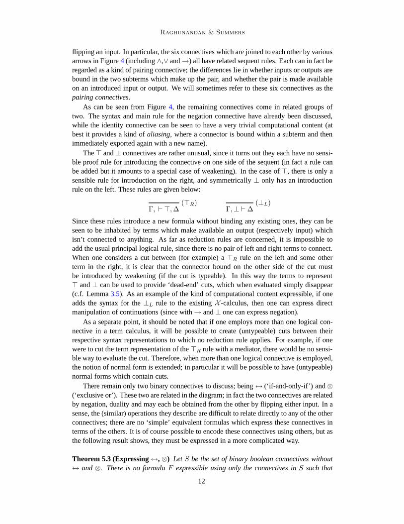
The⊤ and⊥ connectives are rather unusual, since it turns out they eachhave no sensi-ble proof rule for introducing the connective on one side of the sequent (in fact a rule canbe added but it amounts to a special case of weakening). In thecase of⊤, there is only asensible rule for introduction on the right, and symmetrically ⊥ only has an introductionrule on the left. These rules are given below:

(⊤R)Γ, ⊢ ⊤,∆

(⊥L)Γ,⊥ ⊢ ∆

Since these rules introduce a new formula without binding any existing ones, they can beseen to be inhabited by terms which make available an output (respectively input) whichisn’t connected to anything. As far as reduction rules are concerned, it is impossible toadd the usual principal logical rule, since there is no pair of left and right terms to connect.When one considers a cut between (for example) a⊤R rule on the left and some otherterm in the right, it is clear that the connector bound on the other side of the cut mustbe introduced by weakening (if the cut is typeable). In this way the terms to represent⊤ and⊥ can be used to provide ‘dead-end’ cuts, which when evaluatedsimply disappear(c.f. Lemma3.5). As an example of the kind of computational content expressible, if oneadds the syntax for the⊥L rule to the existingX -calculus, then one can express directmanipulation of continuations (since with→ and⊥ one can express negation).

As a separate point, it should be noted that if one employs more than one logical con-nective in a term calculus, it will be possible to create (untypeable) cuts between theirrespective syntax representations to which no reduction rule applies. For example, if onewere to cut the term representation of the⊤R rule with a mediator, there would be no sensi-ble way to evaluate the cut. Therefore, when more than one logical connective is employed,the notion of normal form is extended; in particular it will be possible to have (untypeable)normal forms which contain cuts.

There remain only two binary connectives to discuss; being↔ (‘if-and-only-if’) and⊗(‘exclusive or’). These two are related in the diagram; in fact the two connectives are relatedby negation, duality and may each be obtained from the other by flipping either input. In asense, the (similar) operations they describe are difficultto relate directly to any of the otherconnectives; there are no ‘simple’ equivalent formulas which express these connectives interms of the others. It is of course possible to encode these connectives using others, but asthe following result shows, they must be expressed in a more complicated way.

Theorem 5.3 (Expressing↔,⊗) LetS be the set of binary boolean connectives without↔ and⊗. There is no formulaF expressible using only the connectives inS such that

12


both:

(a) F is logically equivalent to eitherA↔B or A⊗B.

(b) A andB occur inF only once.

Remark 5.4 In contrast, all of the connectives inS can be expressed in terms of otherconnectives inS usingA andB only once; in a sense they can be expressed more directlythan the two connectives in question.

The following technical lemma allows us to show the theorem:

Lemma 5.5 (Removing⊤,⊥ and ID ) If F is a formula constructed using the binary con-nectives, and the propositional variablesA andB, then there exists a formulaG such that:

(a) G ≡ F .

(b) A andB each occur inG no more times than they do inF .

(c) No other propositional variables occur inG.

(d) G does not use theID connective.

(e) EitherG does not mention⊤ and⊥, or eitherG = ⊤ or G = ⊥.

Proof. Just the idea of the proof is given here. Firstly, it is clear that any uses of theIDconnective can be simply removed while maintaining an equivalent formula. One can thendefine a rewrite system (using equivalences) to eliminate all occurrences of⊤ and⊥ whichare underneath another connective. For example, one rewritesA∧⊤ to A, andA→⊥ to¬A. It is easy to show the rewrite system is strongly normalising, and that its normal formssatisfy the criteria listed. 2

Proof. [of Theorem5.3] Suppose that such a formulaF exists and seek a contradiction.ClearlyF cannot be equivalent to⊤ or ⊥. Hence, by Lemma5.5 there exists a formulaG ≡ F which doesn’t mention⊤,⊥ or ID, and mentionsA andB at most once. Note that↔ and⊗ are respectively the parity function on two arguments, and its negation. Since thetruth value ofA↔B depends on the truth values of both arguments,Gmust mentionA andB exactly once. Now remove any double-negations which may occur, to obtain a formulaG′. Without loss of generalityG′ is of the form◦1((◦2A) • (◦3B)), where• is one of∧,∨, ↑, ↓,→,−, while ◦1, ◦2, ◦3 are positions in which¬ may or may not occur. Withoutloss of generality again, by assumptionG′ ≡ A↔B (the case for⊗ is identical).A↔Balways depends on the values of bothA andB to evaluate its result, whereas by Theorem5.1(3), • does not always depend on both the values of its arguments, thereforeG′ does notalways depend on the values of bothA andB. Contradiction. 2

This theorem suggests that the two connectives↔ and⊗ may have some interestingcomplexity which the other binary connectives do not. It seems natural to investigate thecomputational content of these two connectives, which appears not to have been attemptedso far in the literature. In particular, no cut-eliminationrule (or analogously, proof reductionrule in a Natural Deduction setting) seems to have been defined for these connectives. It isthese concerns which motivate the next section.

13


6 Interpreting if-and-only-if

In this section we study the computational behaviour of the logical connective ‘if-and-only-if’ (‘iff’ for short) that evaluates to true exactly when itstwo arguments have the same truthvalue. We could equally have chosen to study the negation of this connective ‘exclusive-or’,whoseX -style term representations will be almost the same except that the free connectorthat is introduced in each term will be of the opposite kind (input versus output).

We are able to determine the form of the left and right introduction rules for the iffconnective via the equivalenceA↔B ≡ ¬(A∨B)∨(A∧B) for example. From this, wecan construct derivations whose conclusions introduce this compound formula on the leftand right of a sequent. (Detailed proofs are given in Appendix A).

Condensing these derivations gives us the (↔L) and (↔R) introduction rules shown inFigure6, which we can inhabit withX -style terms in the usual way. We write the corre-sponding ‘iff-left’ and ‘iff-right’ terms as[Mµσ [y] ijN ] and[xP α, zQδ].γ respectively.

Γ ⊢ A,B,∆ Γ, A,B ⊢ ∆(↔L)

Γ, (A↔B) ⊢ ∆

Γ, A ⊢ B,∆ Γ, B ⊢ A,∆(↔R)

Γ ⊢ (A↔B),∆

Fig. 6.↔L and↔R introduction rules

The principal logical rule for iff should transform a proof that cuts together an (↔R)formula with an (↔L) formula, or inX notation,

([xP α, zQδ].γ)γ † y([Mµσ [y] ijN ]) , γ, y are introduced.

The reduct is not straightforward to determine. The rules for the iff connective each bindtwo inputs andtwo outputs, and each rule has two subterms. We observe a striking re-semblance between these terms and those used to represent the implication connective(i.e. the syntax ofX , Definition 3.1). The iff-right term is reminiscent of an exportterm, except two ‘functions’ are available over the same interface rather than one (n.b.A↔B≡(A→B)∧(B→A)). The iff-left term is reminiscent of a mediator with two bindersover each of its subterms instead of one.

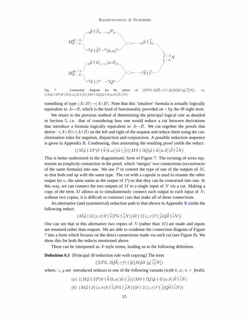
In the case of a mediator,Rψ [l] kS, we seek to connect the termsR andS togethervia the provided connectors. In general, connectingψ to k directly would result in therestriction that our ‘implications’ must be of the formA→A; instead we allow the body ofan export to be inserted to ‘mediate’ between these two subterms. If we think of the iff-leftterm as a kind of mediator, the problem we must solve is again that of connecting outputsand inputs between the termsM andN . However, even in the general case,M andN havebound connectors with types in common; it would seem that we have everything we needto connect these terms together directly.Mµ appears to connect well withiN andMσ

appears to connect well withjN .In general this cannot be done, since the underlying proof sequents interpret the types

of the two inputs as formulas that are read conjunctively, and the types of the two outputsas formulas that are read disjunctively. In this context,M offers a value of typeA or avalue of typeB (loosely a value of typeA∨B) while N requires both a value of typeAand a value of typeB (loosely, requires a value of typeA∧B). Therefore, the problemwe must solve in trying to join these two proofs is essentially that of determining how wecan convert from a value of typeA∨B to a value of typeA∧B, i.e. we intuitively need

14


Aµ † xA AP B

Mµ : Aσ : B Bα † jB

Bσ † kB B〈k.α〉Bj : Bi : AN

Aµ † wA A〈w.δ〉A

Mµ : Aσ : B

Aδ † iA

Bσ † zB BQA

Fig. 7. Connection diagram for the reduct of([bxP bα, bzQbδ].γ)bγ † by([M bµbσ [y]bibjN ]), i.e.((M bµ † bxP )bσ †bk〈k.α〉)bα †bj(((Mbσ † bzQ)bµ † bw〈w.δ〉)bδ †biN)

something of type(A∨B)→(A∧B). Note that this ‘intuitive’ formula is actually logicallyequivalent toA↔B, which is the kind of functionality provided onγ by the iff-right term.

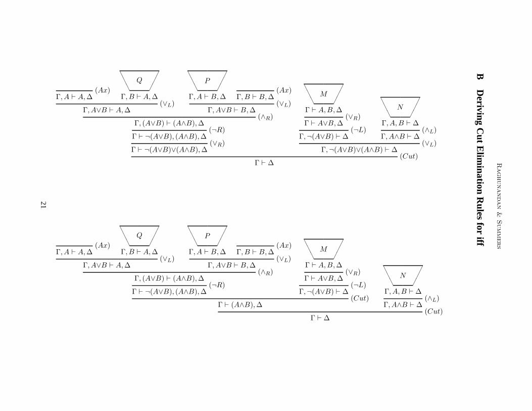
We return to the previous method of determining the principal logical rule as detailedin Section5, i.e. that of considering how one would reduce a cut between derivationsthat introduce a formula logically equivalent toA↔B. We cut together the proofs thatderive¬(A∨B)∨(A∧B) on the left and right of the sequent and reduce them using the cut-elimination rules for negation, disjunction and conjunction. A possible reduction sequenceis given in AppendixB. Condensing, then annotating the resulting proof yields the reduct:

((Mµ † xP )σ † k〈k.α〉)α † j(((Mσ † zQ)µ † w〈w.δ〉)δ † iN)

This is better understood in the diagrammatic form of Figure7. The twisting of wires rep-resents an (implicit) contraction in the proof, which ‘merges’ two connections (occurrencesof the same formula) into one. We useP to convert the type of one of the outputs ofM ,so that both end up with the same type. The cut with a capsule isused to rename the otheroutput (toα, the same name as the output ofP ) so that they can be contracted into one. Inthis way, we can connect the two outputs ofM to a single input ofN via a cut. Making acopy of the termM allows us to simultaneously connect each output to each input of N ;without two copies, it is difficult to construct cuts that make all of these connections.

An alternative (and symmetrical) reduction path to that shown in AppendixB yields thefollowing reduct.

(Mµ † x(〈x.π〉π † i(Pα † jN)))σ † z(〈z.τ〉τ † j(Qδ † iN))

One can see that in this alternative two copies ofN (rather thanM ) are made and inputsare renamed rather than outputs. We are able to condense the connection diagram of Figure7 into a form which focuses on the direct connections made via each cut (see Figure8). Weshow this for both the reducts mentioned above.

These can be interpreted asX -style terms, leading us to the following definition.

Definition 6.1 [Principal iff-reduction rule with copying] The term

([xP α, zQδ].γ)γ † y([Mµσ [y] ijN ])

where,γ, y are introducedreduces to one of the following variants (withk,w, π, τ fresh).

(a) ((Mµ † xP )σ † k〈k.α〉)α † j(((Mσ † zQ)µ † w〈w.δ〉)δ † iN)

(b) (Mµ † x(〈x.π〉π † i(Pα † jN)))σ † z(〈z.τ〉τ † j(Qδ † iN))

15


Mµ:Aσ:B

x:APα:B

z:BQ

δ:A

i:Aj:BN M

µ:Aσ:B

x:APα:B

z:BQ

δ:A

i:Aj:BN

Fig. 8. Simplified connection diagrams for the reducts of Definition 6.1

As mentioned previously, a copy of eitherM orN is used to facilitate the connectionof each output ofM to each input ofN . The question arises of whether this copying isnecessary. One of the graphs shown in Figure8 renames both outputs ofM while the otherrenames both inputs ofN . We sought to explore other ways in whichM andN could beconnected and more specifically, whether it would be possible to obtain a reduct for theprincipal logical rule for↔ which did not require copying. We sought to distribute theconnections in a more symmetrical fashion because we believed that the copying was onlynecessary due to the large number of connections being made with one term or the other.We discovered a solution where we renameoneoutput inM andone input in N . Thisleads to the diagrams shown in Figure9. The reader can verify that a path exists from eachoutput ofM to to each input ofN .

Mµ:Aσ:B

x:APα:B

z:BQ

δ:A

i:Aj:BN M

µ:Aσ:B

x:APα:B

z:BQ

δ:A

i:Aj:BN

Fig. 9. Simplified Connection Diagrams for the Reducts of Definition 6.2

This leads us to a simpler definition for the principal logical rule.

Definition 6.2 [Simplified Principal iff-reduction Rule] The term

([xP α, zQδ].γ)γ † y([Mµσ [y] ijN ])

where,γ, y introducedandk, π freshreduces to one of the following variants.

(a) ((Mµ † xP )σ † k〈k.α〉)α † z(〈z.π〉π † j(Qδ † iN))

(b) ((Mσ † zQ)µ † k〈k.δ〉)δ † x(〈x.π〉π † i(Pα † jN))

These reducts will be significantly cheaper to evaluate thanthose given in Definition6.1since an extra copy ofM (orN ) is not required and fewer cuts are needed to represent allthe necessary connections. From now on, we will use this version of the principal logicalrule for iff.

6.1 Simulating other connectives

If a logical connective is able to express another connective, then it is straightforward tosimulate the computational content of the latter connective in a term-calculus corresponding

16


to the former. The only logical connectives expressible by (↔) are (⊤) and (ID), whichmight lead us to believe its simulation capabilities in thissense are limited. However, wefind this is not the case; in fact we are able to simulate the reductions associated with severalother connectives, i.e. we can encode the syntax for these other connectives in such a waythat reductions are preserved. When this is the case, we say we cancomputationally expressthe connective (which may or may not be expressible in a logical sense).

If we look at the iff-terms themselves, we find they provide a wealth of input and outputconnectors arranged in different combinations over a number of subterms. We also observethat the principal logical rule (see Definition6.2) offers a number of interactions betweenthese different subterms, giving scope for modelling a variety of computational behaviour,some of which may be new.

As an example of a connective which can be computationally expressed (but not logi-cally expressed) by iff, we show how to express the syntax andreduction behaviour of theX -calculus (based on the implication connective) in a term calculus based on the iff con-nective (which we callX↔). We give the definition of this new calculus below. For brevitywe omit the activated cuts, which should be treated analogously.

Definition 6.3 [Syntax for the calculus,X↔]

M,N ::= 〈x.α〉 | [Mµσ [z] ijN ] | [xMα, zNδ].γ | Mα † xN

axiom iff-left iff-right cut

The typing rules for terms of theX↔-calculus are given below.

Definition 6.4 [Typing rules forX↔]

(Ax)〈x.α〉 ··· Γ, x:A ⊢ α:A,∆

M ··· Γ ⊢ α:A,∆ N ··· Γ, x:A ⊢ ∆(Cut)

Mα † xN ··· Γ ⊢ ∆

M ··· Γ ⊢ µ:A,α:B,∆ N ··· Γ, i:A, j:B ⊢ ∆(↔L)

[Mµσ [z] ijN ] ··· Γ, z:(A↔B) ⊢ ∆

M ··· Γ, x:A ⊢ α:B,∆ N ··· Γ, z:B ⊢ δ:A,∆(↔R)

[xMα, zNδ].γ ··· Γ ⊢ γ:(A↔B),∆

As remarked earlier, the iff-left term is reminiscent of a mediator with two binders overeach of its subterms rather than one, and the iff-right term is reminiscent of an export,except that two ‘functions’ are available over the same interface rather than one. With thisobservation in mind, we move towards an encoding of theX -calculus inX↔.

We can sensibly assume that when encoding the export term into an iff-right term[xP α, zQδ].γ, we require only one of the two subterms, sayP . This leaves the question ofwhat we should do withQ. By makingQ the capsule〈y.δ〉, we can give an encoding thatis sound (no undesired reductions are possible) providing that we restrict the reduction toalways use the first variant of the principal logical rule given in Definition6.2. This doesnot seem a severe restriction; one might view this as a strategy on the reduction (one alwayshas the choice of which variant of the principal iff rule to use). Our encoding is as follows.

17


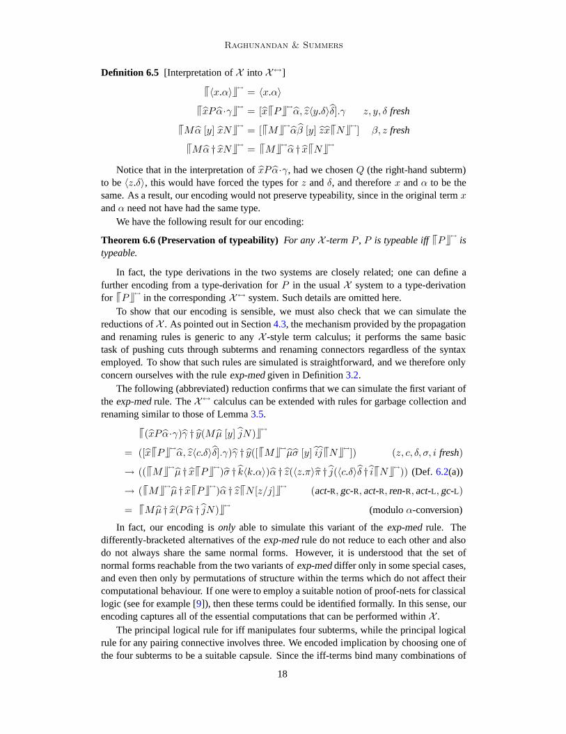
Definition 6.5 [Interpretation ofX intoX↔]

⌈⌈〈x.α〉⌋⌋↔

= 〈x.α〉

⌈⌈xP α·γ⌋⌋↔

= [x⌈⌈P ⌋⌋↔

α, z〈y.δ〉δ].γ z, y, δ fresh

⌈⌈Mα [y] xN⌋⌋↔

= [⌈⌈M⌋⌋↔

αβ [y] zx⌈⌈N⌋⌋↔

] β, z fresh

⌈⌈Mα † xN⌋⌋↔

= ⌈⌈M⌋⌋↔

α † x⌈⌈N⌋⌋↔

Notice that in the interpretation ofxPα·γ, had we chosenQ (the right-hand subterm)to be〈z.δ〉, this would have forced the types forz andδ, and thereforex andα to be thesame. As a result, our encoding would not preserve typeability, since in the original termxandα need not have had the same type.

We have the following result for our encoding:

Theorem 6.6 (Preservation of typeability) For anyX -termP , P is typeable iff⌈⌈P ⌋⌋↔

istypeable.

In fact, the type derivations in the two systems are closely related; one can define afurther encoding from a type-derivation forP in the usualX system to a type-derivationfor ⌈⌈P ⌋⌋

↔

in the correspondingX↔ system. Such details are omitted here.To show that our encoding is sensible, we must also check thatwe can simulate the

reductions ofX . As pointed out in Section4.3, the mechanism provided by the propagationand renaming rules is generic to anyX -style term calculus; it performs the same basictask of pushing cuts through subterms and renaming connectors regardless of the syntaxemployed. To show that such rules are simulated is straightforward, and we therefore onlyconcern ourselves with the ruleexp-medgiven in Definition3.2.

The following (abbreviated) reduction confirms that we can simulate the first variant oftheexp-medrule. TheX↔ calculus can be extended with rules for garbage collection andrenaming similar to those of Lemma3.5.

⌈⌈(xP α·γ)γ † y(Mµ [y] jN)⌋⌋↔

= ([x⌈⌈P ⌋⌋↔

α, z〈c.δ〉δ].γ)γ † y([⌈⌈M⌋⌋↔

µσ [y] ij⌈⌈N⌋⌋↔

]) (z, c, δ, σ, i fresh)

→ ((⌈⌈M⌋⌋↔

µ † x⌈⌈P ⌋⌋↔

)σ † k〈k.α〉)α † z(〈z.π〉π † j(〈c.δ〉δ † i⌈⌈N⌋⌋↔

)) (Def. 6.2(a))

→ (⌈⌈M⌋⌋↔

µ † x⌈⌈P ⌋⌋↔

)α † z⌈⌈N [z/j]⌋⌋↔

(act-R,gc-R,act-R, ren-R,act-L,gc-L)

= ⌈⌈Mµ † x(Pα † jN)⌋⌋↔

(moduloα-conversion)

In fact, our encoding isonly able to simulate this variant of theexp-medrule. Thedifferently-bracketed alternatives of theexp-medrule do not reduce to each other and alsodo not always share the same normal forms. However, it is understood that the set ofnormal forms reachable from the two variants ofexp-meddiffer only in some special cases,and even then only by permutations of structure within the terms which do not affect theircomputational behaviour. If one were to employ a suitable notion of proof-nets for classicallogic (see for example [9]), then these terms could be identified formally. In this sense, ourencoding captures all of the essential computations that can be performed withinX .

The principal logical rule for iff manipulates four subterms, while the principal logicalrule for any pairing connective involves three. We encoded implication by choosing one ofthe four subterms to be a suitable capsule. Since the iff-terms bind many combinations of

18


inputs and outputs, we can suitably restrict them to computationally express other pairingconnectives in a similar way. We are able to do this for the logical connectives∧ and↑ up tothe same limitations as discussed above for implication. Additionally, this can be achievedfor the negation connective without limitations.

While the iff connective is unable to logically express the connectives→, ∧, ↑, ¬, weare able to simulate the significant computational behaviour of their corresponding termcalculi. Similarly, the⊗ connective is able to simulate the computational behaviourfor thedual pairing connectives−, ∨, ↓ and again for the connective¬.

7 Conclusions and Future Work

This work has provided an analysis of the issues involved in deriving term calculi to cor-respond with arbitrary choices of logical connective. We have shown various general tech-niques for deriving suitable syntax, reduction rules and (to some extent) computationalcontent corresponding with the inclusion of a logical connective of interest.

The analysis of logical connectives purely in terms of the movement of their inputs andoutputs seems to yield interesting results, and this shouldbe looked at more closely. Forexample, we hypothesise that a term calculus can express non-terminating terms if and onlyif it contains a connective which can ‘swap’ an input for an output.

Our investigation into the↔ connective has shown that much more can be expressedthan we first thought, and this directly relates to the inputsand outputs present. A moregeneral investigation of the computational content of thisconnective (in particular, anyexamples which are not neatly expressed with other connectives) is the subject of futurework. Our simulation result forX would also be strengthened by the formalisation of asuitable notion of equivalence onX -terms, which is likely to relate to Kleene permutationsand/or proof-nets.

8 Acknowledgements

We would like to thank Steffen van Bakel, Luca Cardelli, Dorian Gaertner, David Gross,Pierre Lescanne and DragisaZunic for many interesting discussions on the subject of thispaper.

References

[1] Tristan Crolard. A formulae-as-types interpretation of subtractive logic.Journal of Logic and Computation, 14(4):529–570, 2004.

[2] Pierre-Louis Curien and Hugo Herbelin. The duality of computation. InProc. ICFP’00, pages 233–243. ACM, 2000.

[3] Gerhard Gentzen. Untersuchungen uber das logische Schliessen. Mathematische Zeitschrift, 39:176–210, 405–431,1934.

[4] Hugo Herbelin. A lambda-calculus structure isomorphicto Gentzen-style sequent calculus structure. InProc. CSL ’94,volume 933 ofLNCS, pages 61–75. Springer, 1994.

[5] S.C. Kleene.Introduction to Metamathematics. North-Holland, 1952.

[6] Stephane Lengrand. Call-by-value, call-by-name, andstrong normalization for the classical sequent calculus. InENTCS, volume 86 ofentcs. Elsevier, 2003.

[7] P.B. Levy. Jumbo lambda-calculus. InProc. ICALP’06, LNCS. Springer-Verlag, 2006.

19


[8] M. Parigot. An algorithmic interpretation of classicalnatural deduction. InProc. LPAR’92, volume 624 ofLNCS, pages190–201. Springer-Verlag, 1992.

[9] Edmund Robinson. Proof nets for classical logic.J. Logic Comput., 13(5):777–797, 2003. Special issue: Semanticfoundations of proof-search.

[10] Alexander J. Summers and Steffen van Bakel. Approachesto polymorphism in classical sequent calculus. InESOP’06,pages 84–99, 2006.

[11] Christian Urban.Classical Logic and Computation. PhD thesis, University of Cambridge, 2000.

[12] S. van Bakel, S. Lengrand, and P. Lescanne. The languageX : circuits, computations and classical logic. InProc.ICTCS’05, 2005.

[13] Steffen van Bakel and Jayshan Raghunandan. Explicit alpha conversion and garbage collection inX . Unpublished,April 2006.

[14] Philip Wadler. Call-by-value is dual to call-by-name.In ICFP’03, pages 189–201. ACM Press, 2003.

A Deriving iff rules using A↔B ≡ ¬(A∨B) ∨ (A∧B)

Proof ofΓ,¬(A∨B) ∨ (A∧B) ⊢ ∆:

AAA

��

�Γ ⊢ A,B,∆

(∨R)Γ ⊢ A∨B,∆

(¬L)Γ,¬(A∨B) ⊢ ∆

AAA

��

�Γ, A,B ⊢ ∆

(∧L)Γ, A∧B ⊢ ∆

(∨L)Γ,¬(A∨B) ∨ (A∧B) ⊢ ∆

Proof ofΓ ⊢ ¬(A∨B) ∨ (A∧B),∆:

(Ax)Γ, A ⊢ A,∆

AAA

��

�Γ, B ⊢ A,∆

(∨L)Γ, A∨B ⊢ A,∆

AAA

��

�Γ, A ⊢ B,∆

(Ax)Γ, B ⊢ B,∆

(∨L)Γ, A∨B ⊢ B,∆

(∧R)Γ, (A∨B) ⊢ (A∧B),∆

(¬R)Γ ⊢ ¬(A∨B), (A∧B),∆

(∨R)Γ ⊢ ¬(A∨B) ∨ (A∧B),∆

20

Raghunandan

&Summers

BD

erivingC

utElim

inationR

ulesforiff

(Ax)Γ, A ⊢ A,∆

AAA

��

�Q

Γ, B ⊢ A,∆(∨L)

Γ, A∨B ⊢ A,∆

AAA

��

�P

Γ, A ⊢ B,∆(Ax)

Γ, B ⊢ B,∆(∨L)

Γ, A∨B ⊢ B,∆(∧R)

Γ, (A∨B) ⊢ (A∧B),∆(¬R)

Γ ⊢ ¬(A∨B), (A∧B),∆(∨R)

Γ ⊢ ¬(A∨B)∨(A∧B),∆

AAA

��

�M

Γ ⊢ A,B,∆(∨R)

Γ ⊢ A∨B,∆(¬L)

Γ,¬(A∨B) ⊢ ∆

AAA

��

�N

Γ, A,B ⊢ ∆(∧L)

Γ, A∧B ⊢ ∆(∨L)

Γ,¬(A∨B)∨(A∧B) ⊢ ∆(Cut)

Γ ⊢ ∆

(Ax)Γ, A ⊢ A,∆

AAA

��

�Q

Γ, B ⊢ A,∆(∨L)

Γ, A∨B ⊢ A,∆

AAA

��

�P

Γ, A ⊢ B,∆(Ax)

Γ, B ⊢ B,∆(∨L)

Γ, A∨B ⊢ B,∆(∧R)

Γ, (A∨B) ⊢ (A∧B),∆(¬R)

Γ ⊢ ¬(A∨B), (A∧B),∆

AAA

��

�M

Γ ⊢ A,B,∆(∨R)

Γ ⊢ A∨B,∆(¬L)

Γ,¬(A∨B) ⊢ ∆(Cut)

Γ ⊢ (A∧B),∆

AAA

��

�N

Γ, A,B ⊢ ∆(∧L)

Γ, A∧B ⊢ ∆(Cut)

Γ ⊢ ∆

21

Raghunandan

&Summers

AAA

��

�M

Γ ⊢ A,B,∆(∨R)

Γ ⊢ A∨B,∆

(Ax)Γ, A ⊢ A,∆

AAA

��

�Q

Γ, B ⊢ A,∆(∨L)

Γ, A∨B ⊢ A,∆

AAA

��

�P

Γ, A ⊢ B,∆(Ax)

Γ, B ⊢ B,∆(∨L)

Γ, A∨B ⊢ B,∆(∧R)

Γ, (A∨B) ⊢ (A∧B),∆(Cut)

Γ ⊢ (A∧B),∆

AAA

��

�N

Γ, A,B ⊢ ∆(∧L)


Γ ⊢ ∆

AAA

��

�M

Γ ⊢ A,B,∆(∨R)

Γ ⊢ A∨B,∆

(Ax)Γ, A ⊢ A,∆

AAA

��

�Q

Γ, B ⊢ A,∆(∨L)

Γ, A∨B ⊢ A,∆(Cut)

Γ,⊢ A,∆

AAA

��

�M

Γ ⊢ A,B,∆(∨R)

Γ ⊢ A∨B,∆

AAA

��

�P

Γ, A ⊢ B,∆(Ax)

Γ, B ⊢ B,∆(∨L)

Γ, A∨B ⊢ B,∆(Cut)

Γ ⊢ B,∆(∧R)

Γ ⊢ (A∧B),∆

AAA

��

�N

Γ, A,B ⊢ ∆(∧L)


Γ ⊢ ∆

22

Raghunandan

&Summers

AAA

��

�M

Γ ⊢ A,B,∆

AAA

��

�Q

Γ, B ⊢ A,∆(Cut)

Γ ⊢ A,∆(Ax)

Γ, A ⊢ A,∆(Cut)

Γ ⊢ A,∆

AAA

��

�M

Γ ⊢ A,B,∆

AAA

��

�P

Γ, A ⊢ B,∆(Cut)

Γ ⊢ B,∆(Ax)

Γ, B ⊢ B,∆(Cut)

Γ ⊢ B,∆(∧R)

Γ ⊢ (A∧B),∆

AAA

��

�N

Γ, A,B ⊢ ∆(∧L)


Γ ⊢ ∆

AAA

��

�M

Γ ⊢ A,B,∆

AAA

��

�P

Γ, A ⊢ B,∆(Cut)

Γ ⊢ B,∆(Ax)

Γ, B ⊢ B,∆(Cut)

Γ ⊢ B,∆

AAA

��

�M

Γ ⊢ A,B,∆

AAA

��

�Q

Γ, B ⊢ A,∆(Cut)

Γ ⊢ A,∆(Ax)

Γ, A ⊢ A,∆(Cut)

Γ ⊢ A,∆

AAA

��

�N

Γ, A,B ⊢ ∆(Cut)

Γ, B ⊢ ∆(Cut)

Γ ⊢ ∆

23

Documents

On the Computational Representation of Classical Logical ... · Replace this ﬁle with prentcsmacro.styfor your meeting, or with entcsmacro.styfor your meeting. Both can be found