Embed Size (px)
Citation preview
On the Comparison of Stochastic Model Predictive ControlStrategies Applied to a Hydrogen-based Microgrid
P. Velardea,1, L. Valverdeb, J. M. Maestrea, C. Ocampo-Martinezc, C. Bordonsa
aSystem Engineering and Automation Department, School of Engineering, Universidad de Sevilla, 41092Seville, Spain.
bAICIA, School of Engineering, University of Seville, 41092 Seville, Spain.cAutomatic Control Department, Universidad Politecnica de Catalunya, Institut de Robotica i Informatica
Industrial (CSIC-UPC), 08028 Barcelona, Spain.
Abstract
In this paper, a performance comparison among three well-known stochastic modelpredictive control approaches, namely, multi-scenario, tree-based, and chance-constrainedmodel predictive control is presented. To this end, three predictive controllers havebeen designed and implemented in a real renewable-hydrogen-based microgrid. Theexperimental set-up includes a PEM electrolyzer, lead-acid batteries, and a PEM fuelcell as main equipment. The real experimental results show significant differences fromthe plant components, mainly in terms of use of energy, for each implemented tech-nique. Effectiveness, performance, advantages, and disadvantages of these techniquesare extensively discussed and analyzed to give some valid criteria when selecting anappropriate stochastic predictive controller.
Keywords: Hydrogen storage, Microgrid, Model predictive control, Stochasticprocesses, Supply and demand.
1. Introduction
A microgrid is a network of electric generation that may take advantage of sev-eral renewable energy sources: solar panels, wind mini-generators, micro-turbines,fuel cells, among others, to meet the consumer demand by working together with thecentralized grid or autonomously [1]. In a microgrid, the energy is generated only atcertain times, being necessary to provide continuous service to meet the demand at anytime of the day. Challenges arise from the natural intermittency of renewable energysources and the requirements to satisfy the user energy demand [2]. Thereby, storage
Email addresses: [email protected] (P. Velarde), [email protected] (L. Valverde),[email protected] (J. M. Maestre), [email protected] (C. Ocampo-Martinez),[email protected] (C. Bordons)
1Corresponding author
Preprint submitted to Journal of LATEX Templates January 19, 2017
NomenclatureSymbols ez ElectrolyzerE Energy (Wh) fc Fuel cellsE Expected value grid GridF Cumulative distribution function H2 HydrogenJ Cost function net Net powerK Number of scenarios res Renewable energy sourceMHL Metal hydrides level (%) ref ReferenceN Prediction horizon SuperscriptsP Power (W) ∗ Working pointP Probability Measured valueR Reduced number of scenarios AcronymsSOC State of charge (%) ARMA Autoregressive-moving-averageai Weight for state variables CC Chance-constrainedbi Weight for input variables cdf cumulative distributed functionu Input variables IID Independent and identically distributedx State variables KPIs Key performance indicatorsω Disturbances MPC Model predictive control∆P Rate power (Ws−1) MS Multiple-scenariosδx Risk of constraint violation PEM Proton exchange membraneSubscripts PF Perfect forecastbatt Batteries SNEN Spanish national electricity networkdem Demand UPG Utility power grid
TB Tree-based
devices become very important in the operation of this type of systems. Among well-established energy storage technologies, there are batteries, super-capacitors, conven-tional capacitors, etc. In this work, we focus on the use of hydrogen as an energy vectorfor energy storage. Hydrogen, combined with other renewable energy sources, is a safeand viable option to mitigate the problems associated with hydrocarbon combustion be-cause the entire system can be developed as an efficient, clean, and sustainable energysource, as mentioned in [3]. The hydrogen is converted into electrical energy by usingfuel cells; the reverse process, i.e., the transformation of electric energy into hydrogen,is conducted by electrolysis [4], or ethanol reforming [5], among other techniques.
The control problem in a microgrid is to satisfy the electricity demand under eco-nomical and optimal conditions despite the uncertainties and disturbances that mightappear in the processes. Taking into account that there are mathematical models avail-able that represent the main dynamics and the load of these systems [6], and that thecontrol problem here requires the simultaneous handling of constraints, delays, and dis-turbances, model predictive control (MPC) emerges as a solution to this problem. MPCis a control strategy widely used in industry for solving problems considering con-straints on the manipulated and controlled variables, delays, nonlinearities, etc. Verysuccinctly, the main idea of MPC is to obtain a control signal by solving at each time in-stant an optimization problem in a finite prediction horizon based on the system model.Only the first component of the control signal is implemented in the current time step,and the problem is solved in the next time instant in a receding horizon strategy. Dueto its versatility, MPC has become one of the most popular techniques in industrialcontrol applications; see e.g. [7]. From using the MPC approach, different variantsof this technique have been applied to achieve an economical and optimal efficiencyin energy management of a microgrid, see, e.g., [2, 8–13]. The potential benefits of
2
the application of an MPC controller are discussed to solve this control problem in aneconomical manner. A review of the approaches applied for controlling smart gridshave been presented in [14, 15] and references therein.
Uncertainty in the load and generation profiles has been mainly addressed indirectlyin the dispatch problem by using the MPC approach [14]. The classical formulationof MPC does not allow considering systems with uncertainties although some MPCschemes have been proposed to ensure stability and compliance with constraints inthe presence of disturbances [16]. One way to address this problem is by means of theconservative min-max approach, e.g., in [17] control of microgrids using this techniqueis shown. A less conservative approach is the stochastic one, which is based on thedesign of predictive controllers for dynamical systems subject to disturbances and/oruncertainty in terms of the probability that a certain solution is feasible [18], mainlybecause it is not strictly possible to speak about guaranteed feasibility in this context.
Due to the increasing importance that uncertainty plays in the power dispatch ofsmartgrids, stochastic MPC can be used to deal with the uncertainty in the energy de-mand and the renewable generation. At this point, the question of which method pro-vides the best performance to manage the inherent uncertainties in microgrids arises.Although each method provides a different solution to the same problem, a comparisonbetween the available techniques has been missed in the literature up to date. This isindeed the main contribution of this paper. Three popular stochastic MPC techniqueshave been implemented and tested to obtain experimental evidence in a real compari-son framework of their suitability. The criteria to assess the controller performance isbased on specific key performance indicators (KPIs) defined in this work. Also, guide-lines for controller design, tuning, and real-time implementation in a hydrogen-basedmicrogrid are also provided. Finally, the experimental results obtained highlight ad-vantages and weaknesses when coping with disturbances and uncertainties within theclosed loop of a hydrogen-based microgrid.
Therefore, in this paper, three different stochastic-programming-based MPC tech-niques are used to deal with the uncertainty of the power demand and power generation.In the first place, multiple-scenario MPC (MS-MPC) is considered, which consists incalculating a single control sequence that takes into account different possible evolu-tions of the process disturbances. Hence, the control sequence calculated has a certaindegree of robustness against the potential realizations of the uncertainties. This ap-proach is used for example in [19] for water systems and in [20, 21] within the contextof the control of smart grids. One of its advantages is that it is possible to calculatebounds on the probability of constraint violation as a function of the number of scenar-ios considered [22].
An alternative to model the uncertainty that is faced by this type of systems isto use rooted trees. The rationale behind this approach is that uncertainty spreads withtime, i.e., it is possible to predict –more accurately– both the energy demand and energyproduction by a renewable source in a short horizon than in a large one. For this reason,the possible evolutions of the disturbances can be confined to a tree. In the tree, thereis a bifurcation point whenever the disturbances branch into two possible trajectories.Consequently, the outcome, the so-called tree-based MPC (TB-MPC), is a rooted treeof control actions. This approach is used for example in [23] for a semi-batch reactorexample, in [24] for the energy management of a renewable hydrogen-based microgrid,
3
and in [25] in the context of water systems.Finally, chance-constrained MPC (CC-MPC) is also considered in this work. CC-
MPC uses an explicit probabilistic modeling of the system disturbances to calculate ex-plicit bounds on the system constraint satisfaction. For instance, [26] presents a chance-constrained two-stage stochastic program for unit commitment with uncertain windpower output and [27] shows an autoregressive-moving-average (ARMA) type predic-tion model for the underlying uncertainties (load/generation) into chance-constrainedfinite-horizon optimal control. An application of this technique in the context of thedrinking water network of the city of Barcelona is reported in [28]. In addition, [29]shows a comparison between MS-MPC, TB-MPC, and CC-MPC approaches appliedto drinking water networks via simulation. Further, this subject has drawn significantinterest; a stochastic optimization model implemented in the context of the control ofmicrogrids can be seen in [30–33] and references therein.
The remainder of the paper is organized as follows. First, a description of the mi-crogrid, its linear model and constraints are shown in Section 2. Section 3 presentsthe optimization problem and the formulation of the considered stochastic MPC tech-niques. The comparative study and the analysis drawn from the experimental results arepresented in Section 4. Finally, in Section 5, the main conclusions and future researchlines are proposed.
2. Case Study Description
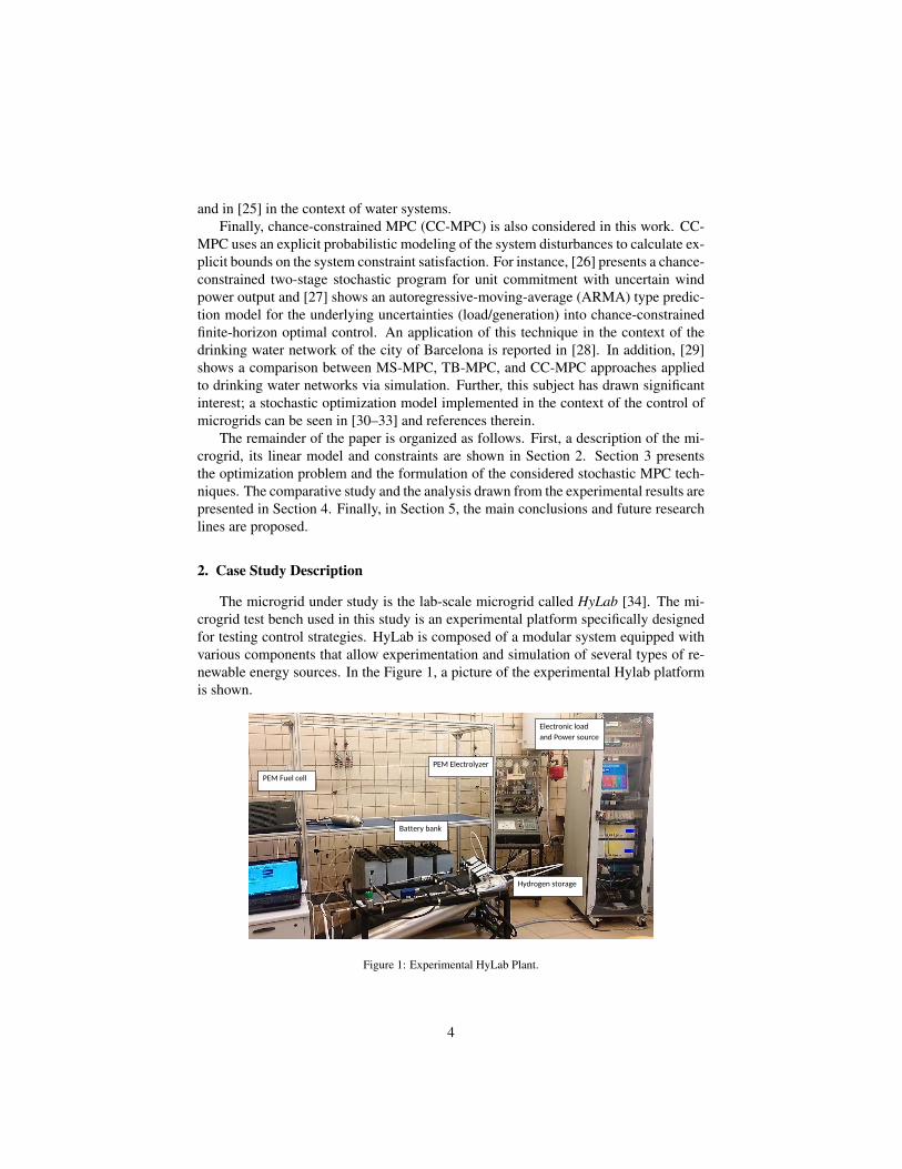
The microgrid under study is the lab-scale microgrid called HyLab [34]. The mi-crogrid test bench used in this study is an experimental platform specifically designedfor testing control strategies. HyLab is composed of a modular system equipped withvarious components that allow experimentation and simulation of several types of re-newable energy sources. In the Figure 1, a picture of the experimental Hylab platformis shown.
PEM Electrolyzer
PEM Fuel cell
Battery bank
Hydrogen storage
Electronic load
and Power source
Figure 1: Experimental HyLab Plant.
4
The system consists of a solar field, emulated by an electronic power source, whichproduces electricity to supply the electronic load. Any excess of power can be eitherstored in a battery bank or derived to the electrolyzer. If the power obtained from re-newable energy is not enough, both the fuel cell and the battery bank can support theload, which is emulated electronically. This type of hybrid storage operation allowsimplementing strategies in separated times scales: the battery can either absorb or con-tribute to balance small amounts of energy in fast transient periods while the hydrogenpath complements larger variations [35]. The microgrid can work either connected tothe utility network or as an isolated system. The Hydrogen Path is composed of threesubsystems: the electrolyzer, which is proton exchange membrane (PEM) type [36],for producing hydrogen; a metal-hydride hydrogen storage tank; and finally a PEMfuel cell [37, 38] that provides power to the loads/batteries. It is important to noticethat both subsystems –electrolyzer and fuel cell– cannot work simultaneously. DC/DCpower converters are used as power interfaces that allow energy transfer between dif-ferent distributed generation units. The equipment is connected to 48 VDC bus that isheld by the battery bank. Table 1 presents the nominal values of the HyLab equipment.
Table 1: HyLab equipment.
Equipment Nominal Value
Electronic power source 6 kWElectronic load source 2.5 kWPEM fuel cell 1.2 kWPEM electrolyzer 0.23 Nm3h−1 @5barg
1 kWMetal hydrides tank 7 Nm3
5 barBattery bank C120 = 367 AhDC/DC converters 1.5 kW, 1 kW
2.1. Microgrid linear model and constraints
As it can be inferred, behind the experimental setup there is a set of complex non-linear subsystems. The detailed description of sub-models and the physical equationsare out of the scope of this paper. The complete non-linear model of the plant, itssimulation, and validation are presented in [39].
Remark 1. To apply linear MPC techniques is required to find a linear model of thesystem around a working point (x∗, u∗). The identification process for obtaining thelinear model of the plant is developed in [9]. The continuous linear system was dis-cretized using Tustin’s method with a sampling time of 30 s. Also, the working point isgiven by u∗ = [0 kW, 1.75 kW]T and x∗ = [50 %, 50 %]T .
5
The linear discrete-time model of the plant consists of two input variables, PH2(k)
and Pgrid(k), which are measured in kilowatts (kW). Here, PH2(k) represents the
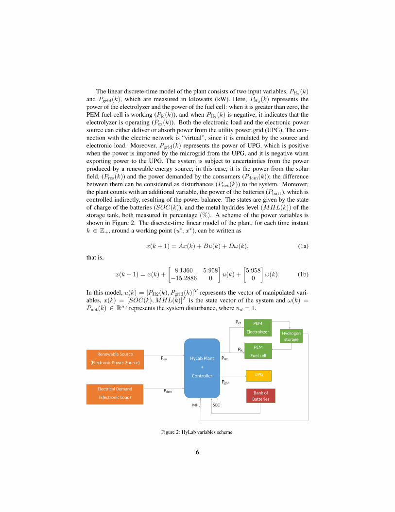
power of the electrolyzer and the power of the fuel cell: when it is greater than zero, thePEM fuel cell is working (Pfc(k)), and when PH2(k) is negative, it indicates that theelectrolyzer is operating (Pez(k)). Both the electronic load and the electronic powersource can either deliver or absorb power from the utility power grid (UPG). The con-nection with the electric network is “virtual”, since it is emulated by the source andelectronic load. Moreover, Pgrid(k) represents the power of UPG, which is positivewhen the power is imported by the microgrid from the UPG, and it is negative whenexporting power to the UPG. The system is subject to uncertainties from the powerproduced by a renewable energy source, in this case, it is the power from the solarfield, (Pres(k)) and the power demanded by the consumers (Pdem(k)); the differencebetween them can be considered as disturbances (Pnet(k)) to the system. Moreover,the plant counts with an additional variable, the power of the batteries (Pbatt), which iscontrolled indirectly, resulting of the power balance. The states are given by the stateof charge of the batteries (SOC(k)), and the metal hydrides level (MHL(k)) of thestorage tank, both measured in percentage (%). A scheme of the power variables isshown in Figure 2. The discrete-time linear model of the plant, for each time instantk ∈ Z+, around a working point (u∗, x∗), can be written as
x(k + 1) = Ax(k) +Bu(k) +Dω(k), (1a)
that is,
x(k + 1) = x(k) +
[8.1360 5.958−15.2886 0
]u(k) +
[5.958
0
]ω(k). (1b)
In this model, u(k) = [PH2(k), Pgrid(k)]T represents the vector of manipulated vari-ables, x(k) = [SOC(k),MHL(k)]T is the state vector of the system and ω(k) =Pnet(k) ∈ Rnd represents the system disturbance, where nd = 1.
Pez
Pfc
Pres PH2
Pgrid
Pdem
MHL SOC
HyLab Plant
+
Controller
Renewable Source
(Electronic Power Source)
Electrical Demand
(Electronic Load)
PEM
Electrolyzer
PEM
Fuel cell
Hydrogen
storage
UPG
Bank of
Batteries
Figure 2: HyLab variables scheme.
6

The system is subject to constraints that avoid equipment damage and guarantee itssafe operation. In particular, the Hydrogen Path –both the electrolyzer and the fuel cell–has constraints for limiting the values of PH2
(k) since its power capacity is limited to0.9 kW; this value reflects some conservatism and it ensures that the hydrogen pathdoes not work at its nominal value to protect the equipment. In this way, a longerlifespan is expected. Also, the Hydrogen Path has a dead zone between −0.1 kWand 0.1 kW that ensures a minimum production of power from both the electrolyzerand the fuel cell. The constraints for Pgrid(k) correspond to physical limitations of theelectronic units. Furthermore, it is necessary to include constraints on their incrementalsignals ∆PH2
(k) and ∆Pgrid(k), to guarantee the physical safety of the equipment.These constraints are mathematically expressed as follows:
− 0.9 kW ≤ PH2(k) ≤ 0.9 kW, (2a)
− 2.5 kW ≤ Pgrid(k) ≤ 2 kW, (2b)
− 20 Ws−1 ≤ ∆PH2(k) ≤ 20 Ws−1, (2c)
− 2.5 kWs−1 ≤ ∆Pgrid(k) ≤ 2 kWs−1. (2d)
Overall constraints have to be considered as hard constraints, since the equipmentlifespan could be drastically reduced. Both the battery bank and the metal hydridesstorage tank have limited capacity to prevent any plant damage by overcharge or un-dercharge. Constraints on SOC(k) guarantee suitable voltage levels in the 48 VDCbus. Also, they protect the battery bank of strong load voltage variations. These stateconstraints are written as
40 % ≤ SOC(k) ≤ 90 %, (3a)10 % ≤MHL(k) ≤ 90 %. (3b)
The input constraints given by (2) can be properly rewritten as
u(k) ∈ U ⊆ Rnu , (4)
with nu = 2, while the state constraints defined by (3) are expressed as
x(k) ∈ X ⊆ Rnx , (5)
with nx = 2. Furthermore, the total power delivered to the load, in order to satisfy theconsumer demand, must satisfy the energy balance
Pdem(k) = PH2(k)− Pbatt(k) + Pgrid(k) + Pres(k). (6)
3. Stochastic MPC formulation for hydrogen-based microgrids
MPC is a strategy based on the explicit use of a dynamical model of the plant topredict the state/output evolution of the process in future time instants along a predic-tion horizonN [7]. The set of future control signals is calculated by the optimization of
7
a criterion or objective function. Only the control signal calculated for the time instantk is applied to the process, whereas the others are withdrawn. One of the advantages ofMPC over other control methods includes the easy extension to the multivariable case.
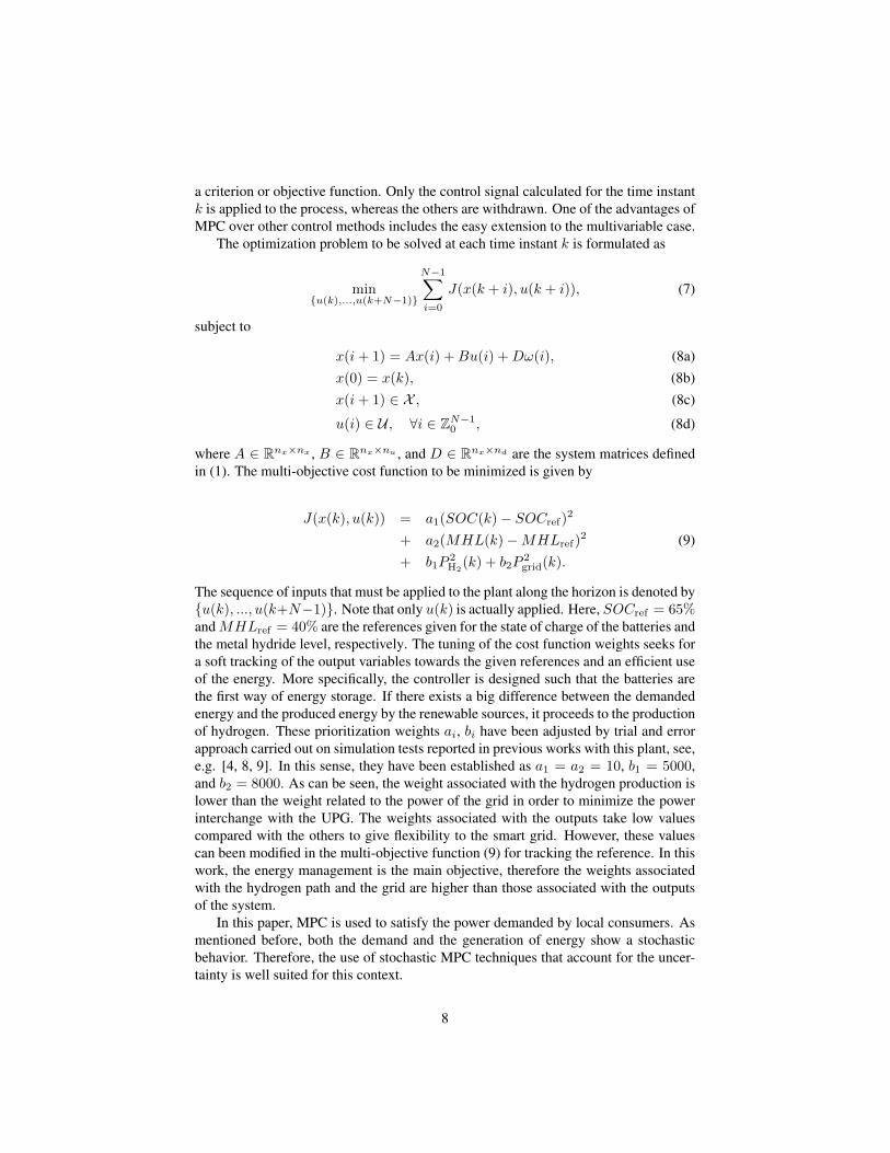
The optimization problem to be solved at each time instant k is formulated as
min{u(k),...,u(k+N−1)}
N−1∑i=0
J(x(k + i), u(k + i)), (7)
subject to
x(i+ 1) = Ax(i) +Bu(i) +Dω(i), (8a)x(0) = x(k), (8b)x(i+ 1) ∈ X , (8c)
u(i) ∈ U , ∀i ∈ ZN−10 , (8d)
where A ∈ Rnx×nx , B ∈ Rnx×nu , and D ∈ Rnx×nd are the system matrices definedin (1). The multi-objective cost function to be minimized is given by
J(x(k), u(k)) = a1(SOC(k)− SOCref)2
+ a2(MHL(k)−MHLref)2 (9)
+ b1P2H2
(k) + b2P2grid(k).
The sequence of inputs that must be applied to the plant along the horizon is denoted by{u(k), ..., u(k+N−1)}. Note that only u(k) is actually applied. Here, SOCref = 65%andMHLref = 40% are the references given for the state of charge of the batteries andthe metal hydride level, respectively. The tuning of the cost function weights seeks fora soft tracking of the output variables towards the given references and an efficient useof the energy. More specifically, the controller is designed such that the batteries arethe first way of energy storage. If there exists a big difference between the demandedenergy and the produced energy by the renewable sources, it proceeds to the productionof hydrogen. These prioritization weights ai, bi have been adjusted by trial and errorapproach carried out on simulation tests reported in previous works with this plant, see,e.g. [4, 8, 9]. In this sense, they have been established as a1 = a2 = 10, b1 = 5000,and b2 = 8000. As can be seen, the weight associated with the hydrogen production islower than the weight related to the power of the grid in order to minimize the powerinterchange with the UPG. The weights associated with the outputs take low valuescompared with the others to give flexibility to the smart grid. However, these valuescan been modified in the multi-objective function (9) for tracking the reference. In thiswork, the energy management is the main objective, therefore the weights associatedwith the hydrogen path and the grid are higher than those associated with the outputsof the system.
In this paper, MPC is used to satisfy the power demanded by local consumers. Asmentioned before, both the demand and the generation of energy show a stochasticbehavior. Therefore, the use of stochastic MPC techniques that account for the uncer-tainty is well suited for this context.
8
Next, the description of the stochastic MPC techniques designed and implementedis presented.
3.1. Multiple-scenarios MPC approach (MS-MPC)The optimization based on scenarios provides an intuitive way to approximate the
solution to the stochastic optimization problem. In order to design the MS-MPC, itis required to know several scenarios with possible evolutions of the energy demandand generation. The scenario forecasts can be obtained either from historical data orby introducing a random scenario generation. The idea behind this approach is thata general control sequence that optimizes all the considered scenarios is calculated,obtaining in this way a certain robustness against the different possible evolutions ofthe disturbances. The scenario-based approach is computationally efficient since itssolution is based on a deterministic convex optimization, even when the original prob-lem is not [40]. One advantage of this approach does not assume a prior knowledgeof the statistical properties that characterize the uncertainty (e.g., a certain probabilityfunction) as generally required in stochastic optimization.
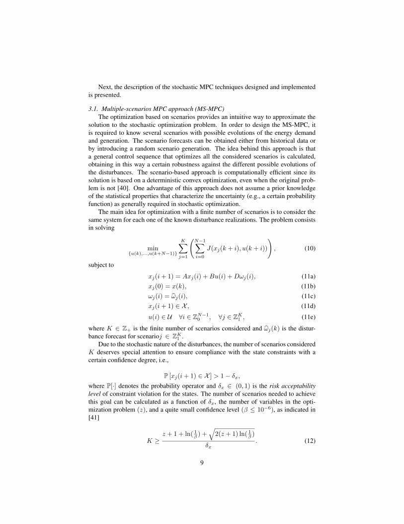
The main idea for optimization with a finite number of scenarios is to consider thesame system for each one of the known disturbance realizations. The problem consistsin solving
min{u(k),...,u(k+N−1)}
K∑j=1
(N−1∑i=0
J(xj(k + i), u(k + i))
), (10)
subject to
xj(i+ 1) = Axj(i) +Bu(i) +Dωj(i), (11a)xj(0) = x(k), (11b)ωj(i) = ωj(i), (11c)xj(i+ 1) ∈ X , (11d)
u(i) ∈ U ∀i ∈ ZN−10 , ∀j ∈ ZK1 , (11e)
where K ∈ Z+ is the finite number of scenarios considered and ωj(k) is the distur-bance forecast for scenarioj ∈ ZK1 .
Due to the stochastic nature of the disturbances, the number of scenarios consideredK deserves special attention to ensure compliance with the state constraints with acertain confidence degree, i.e.,
P [xj(i+ 1) ∈ X ] > 1− δx,where P[·] denotes the probability operator and δx ∈ (0, 1) is the risk acceptabilitylevel of constraint violation for the states. The number of scenarios needed to achievethis goal can be calculated as a function of δx, the number of variables in the opti-mization problem (z), and a quite small confidence level (β ≤ 10−6), as indicated in[41]
K ≥z + 1 + ln( 1
β ) +√
2(z + 1) ln( 1β )
δx. (12)
9
Furthermore, the sample scenarios must meet the following assumptions, as pointedout in [40]:
1. The uncertainties ωj ; ∀j ∈ ZK1 are independent and identically distributed (IID)random variables on a probability space.
2. A “sufficient number” of IID samples of ωj can be obtained, either empiricallyor by a random-number generator.
In this manner, a control sequence is optimized for the system given by (11a),which includes different possible evolutions of the original one. The calculation ofthe controller will result in a unique robust control action that satisfies all the potentialrealizations of the disturbances with a certain probability.
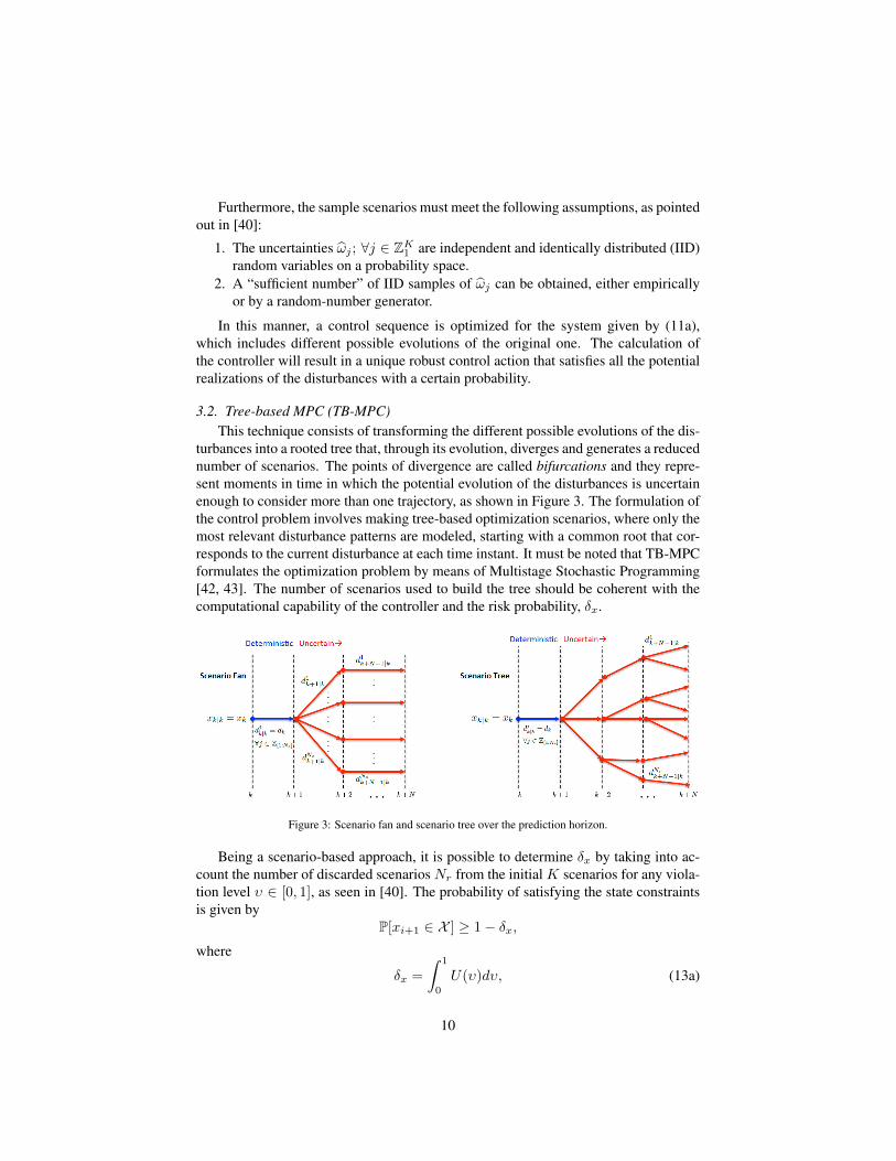
3.2. Tree-based MPC (TB-MPC)This technique consists of transforming the different possible evolutions of the dis-
turbances into a rooted tree that, through its evolution, diverges and generates a reducednumber of scenarios. The points of divergence are called bifurcations and they repre-sent moments in time in which the potential evolution of the disturbances is uncertainenough to consider more than one trajectory, as shown in Figure 3. The formulation ofthe control problem involves making tree-based optimization scenarios, where only themost relevant disturbance patterns are modeled, starting with a common root that cor-responds to the current disturbance at each time instant. It must be noted that TB-MPCformulates the optimization problem by means of Multistage Stochastic Programming[42, 43]. The number of scenarios used to build the tree should be coherent with thecomputational capability of the controller and the risk probability, δx.
Figure 3: Scenario fan and scenario tree over the prediction horizon.
Being a scenario-based approach, it is possible to determine δx by taking into ac-count the number of discarded scenarios Nr from the initial K scenarios for any viola-tion level υ ∈ [0, 1], as seen in [40]. The probability of satisfying the state constraintsis given by
P[xi+1 ∈ X ] ≥ 1− δx,where
δx =
∫ 1
0
U(υ)dυ, (13a)
10

and
U(υ) = min
1,
(Nr + z − 1
Nr
)Nr+z−1∑j=0
(K
j
)υj(1− υ)K−j
. (13b)
In this way, the amount of R used in the optimization problem is calculated asR = K −Nr.
Unlike the MS-MPC approach, each scenario into the tree has its own control sig-nal, which means that more optimization variables are needed. However, given thatthe control signal cannot anticipate events beyond the next bifurcation point, controlsequences for different scenarios must be equal as long as the scenarios do not branchout. As a consequence, the solution of this control problem is a rooted-tree of controlinputs. Notice that only the first component of this tree, which is equal for all the sce-narios, is actually applied. For the design of this controller, the bifurcation points ofthe tree are checked: if they are equal, then the control actions are the same so that boththe number of variables and the computational time can be reduced significantly.
The TB-MPC problem formulation to be solved at each time instant is representedby
min{uj(k),...,uj(k+N−1)}
R∑j=1
(N−1∑i=0
J(xj(k + i), uj(k + i))
), (14)
subject to
xj(i+ 1) = Axj(i) +Buj(i) +Dωj(i), (15a)xj(0) = x(k), (15b)ωj(i) = ωj(i), (15c)
xj(i+ 1) ∈ X , ∀i ∈ ZN−10 , (15d)
uj(i) ∈ U , ∀j ∈ ZR1 . (15e)
In addition, it is necessary to introduce non-anticipative constraints to force the con-troller to compute the control inputs only considering the observed uncertainty beforethe bifurcation points [43]. These constraints are given by
ui(k) = uj(k) if ωi(k) = ωj(k); ∀ i 6= j. (15f)
One way to satisfy (15f) is to introduce equality constraints into the optimizationproblem and solving it with a number of optimization variables defined as z = N×R×nu. Nevertheless, constraints in (15f) can be used to reduce the number of optimizationvariables by removing the redundancy to lower the computational burden.
As said before, a control sequence is optimized for the extended system with adisturbance tree, and only the first component of the input tree is applied to the system.The problem is repeated at each time instant k ∈ Z+.
11

3.3. Chance-Constrained MPC (CC-MPC)
Given that disturbances are stochastic, another way of addressing this problem isusing CC-MPC. The stochastic behavior from the weather conditions and the electricdemand can be addressed by formulating hard constraints into probabilistic constraintsrelated to a risk of constraint violation that determines the degree of the conservatismwhen computing the control inputs. Also, the cost function is expressed as its ex-pected value in the formulation of the optimization problem. A major advantage ofthis approach is that the computational burden is not increased as in the scenario-basedtechniques.
Given that the disturbances in the dynamic model (1a) are stochastic, the state con-straints (5) must be formulated in a probabilistic manner, i.e.,
P[x(i+ 1) ∈ X | Gx ≤ g] > 1− δx. (16)
Here, G ∈ Rnr×nx and g ∈ Rnr . The probabilistic constraints (16), also called chanceconstraints, can be written in two different manners [28]:
• Individual chance constraints that express a probabilistic equivalent for eachconstraint. They are formulated as
P[G(m)x < g(m)] > 1− δx,m, ∀m ∈ Znx1 , (17)
where G(m) and g(m) are the mth row of G and g, respectively. Each mth rowsatisfies its respective δx,m.
• Joint chance constraints, which take into account an unique risk of constraintviolation for all stochastic constraints. They are written as
P[G(m)x < g(m), ∀m ∈ Znx1 ] > 1− δx. (18)
All rows jointly satisfy the unique δx.
The application of (18) along N is necessary to implement the controller. To thisend, it is assumed that the disturbances behave as Gaussian random variables, whichare modeled based on historical data, with a known cumulative distribution function(cdf). The deterministic equivalent of these chance constraints can be formulated asfollows:
P[G(m)x(k + 1) < g(m)] > 1− δx⇔ FG(m)Dω(k)(g(m) −G(m)(Ax(k) +Bu(k))) > 1− δx⇔ G(m)(Ax(k) +Bu(k)) < g(m) − F−1G(m)Dω(k)
(1− δx). (19)
Here, FG(m)Dω(k)(·) represents the cumulative distribution function of the randomvariableG(m)Dω(k), andF−1G(m)Dω(k)
(·) is its inverse cumulative distribution function.Note that the expression (19) is the deterministic equivalent of the chance con-
straints and is built based on historical data.
12

The optimization problem formulation related to the design of the CC-MPC con-troller is stated as
min{u(k),...,u(k+N−1)}
N−1∑i=0
E[J(x(k + i), u(k + i))], (20)
subject to
x(i+ 1) = Ax(i) +Bu(i) +Dω(i), (21a)x(0) = x(k), (21b)ω(i) = ω(i), (21c)
G(m)(Ax(k) +Bu(k)) < g(m) − F−1G(m)Dω(k)(1− δx), (21d)
u(i) ∈ U , ∀i ∈ ZN−11 , (21e)
where E[·] denotes the expected value of the cost function.
4. Results and Discussion
The experiments were conducted in the microgrid described in Section 2 during atrial period of eight hours for each experiment. The controller receives the measuredvariables SOC(k) and MHL(k), which are used to compute the optimal control sig-nals PH2(k) and Pgrid(k)) by means of Simulink Real-Time workshop toolbox. Thecontrol signals are sent to the SCADA via the OPC Matlab Library and finally the PLCcarries out these control actions.
The prediction horizon was N = 5 and the sampling time was 30 s. The selectedweather and load profiles for verifying the performance of the three proposed con-trollers were the scaled difference between the real solar generation and the demandregistered by the Spanish National Electricity Network (SNEN)2 on May 23, 2014.These values were sampled each 3 s and scaled for the microgrid allowable power val-ues, which are shown in Figure 4(a). The initial conditions for all experiments wereSOC(0) = 70% and MHL(0) = 50%.
An issue that deserves particular attention is the amount of scenarios to be con-sidered into the optimization problem. This number should be selected by taking intoaccount a trade-off between robustness and computational burden. In this sense, it ispossible to establish the number of scenarios that guarantees a particular risk level,according to (12), as shown Table 2.
MS-MPC was performed by using the electricity demand and the solar generationregistered during K = 316 different days of one year from historical data, obtainedfrom the SNEN. For these scenarios, it is expected a risk of violation of constraints lessthan δx ≤ 10%. This number of scenarios offers an acceptable risk and ensures a rea-sonable computational burden when solving the optimization problem. Furthermore,
2SNEN demand data can be obtained at: https://demanda.ree.es/movil/peninsula/demanda/total
13
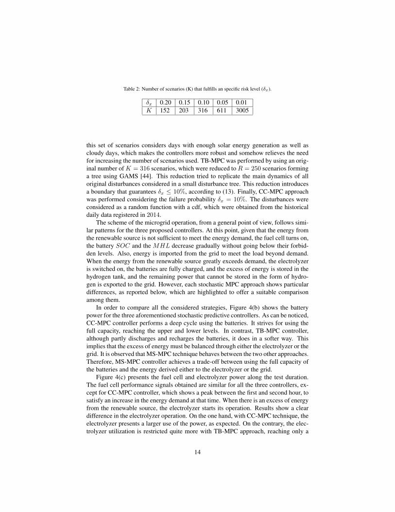
Table 2: Number of scenarios (K) that fulfills an specific risk level (δx).
δx 0.20 0.15 0.10 0.05 0.01K 152 203 316 611 3005
this set of scenarios considers days with enough solar energy generation as well ascloudy days, which makes the controllers more robust and somehow relieves the needfor increasing the number of scenarios used. TB-MPC was performed by using an orig-inal number of K = 316 scenarios, which were reduced to R = 250 scenarios forminga tree using GAMS [44]. This reduction tried to replicate the main dynamics of alloriginal disturbances considered in a small disturbance tree. This reduction introducesa boundary that guarantees δx ≤ 10%, according to (13). Finally, CC-MPC approachwas performed considering the failure probability δx = 10%. The disturbances wereconsidered as a random function with a cdf, which were obtained from the historicaldaily data registered in 2014.
The scheme of the microgrid operation, from a general point of view, follows simi-lar patterns for the three proposed controllers. At this point, given that the energy fromthe renewable source is not sufficient to meet the energy demand, the fuel cell turns on,the battery SOC and the MHL decrease gradually without going below their forbid-den levels. Also, energy is imported from the grid to meet the load beyond demand.When the energy from the renewable source greatly exceeds demand, the electrolyzeris switched on, the batteries are fully charged, and the excess of energy is stored in thehydrogen tank, and the remaining power that cannot be stored in the form of hydro-gen is exported to the grid. However, each stochastic MPC approach shows particulardifferences, as reported below, which are highlighted to offer a suitable comparisonamong them.
In order to compare all the considered strategies, Figure 4(b) shows the batterypower for the three aforementioned stochastic predictive controllers. As can be noticed,CC-MPC controller performs a deep cycle using the batteries. It strives for using thefull capacity, reaching the upper and lower levels. In contrast, TB-MPC controller,although partly discharges and recharges the batteries, it does in a softer way. Thisimplies that the excess of energy must be balanced through either the electrolyzer or thegrid. It is observed that MS-MPC technique behaves between the two other approaches.Therefore, MS-MPC controller achieves a trade-off between using the full capacity ofthe batteries and the energy derived either to the electrolyzer or the grid.
Figure 4(c) presents the fuel cell and electrolyzer power along the test duration.The fuel cell performance signals obtained are similar for all the three controllers, ex-cept for CC-MPC controller, which shows a peak between the first and second hour, tosatisfy an increase in the energy demand at that time. When there is an excess of energyfrom the renewable source, the electrolyzer starts its operation. Results show a cleardifference in the electrolyzer operation. On the one hand, with CC-MPC technique, theelectrolyzer presents a larger use of the power, as expected. On the contrary, the elec-trolyzer utilization is restricted quite more with TB-MPC approach, reaching only a
14

(a) Energy generated by solar panels Pres, demand of energy
Pden, and Pnet corresponding to May 23, 2014.
(b) Battery power.
(c) Fuel cell power and Electrolyzer power. (d) Grid power.
(e) Battery SOC and MHL. (f) Electric power provided by the microgrid compared with the
consumer demand.
Figure 4: Experimental results applying the proposed stochastic MPC approaches.
peak of 200 W, while CC-MPC controller sets the electrolyzer power to nearly 600 W.Regarding TB-MPC approach, it also shows a small ripple; this is explained becausethe controller seeks to primary satisfy the demand and compensate any power unbal-
15
ance in the system. As it has been shown through experimental tests, there are cleardifferences in the way each controller manages the power signals of the electrolyzerand the fuel cell.
Figure 4(d) shows the grid power signal generated by applying the stochastic MPCcontrollers. From the point of view of the network operators (DSO3/TSO4), the useof the UPG is minimized with the CC-MPC approach. In this manner, the impact inthe electrical system generated by the renewable sources present in the microgrid isreduced. On the other hand, for the consumer point of view, it might be convenient notto force the equipment to a deep duty cycle and take advantage of the grid to smooththe power profiles.
Figure 4(e) shows the evolution of the SOC and MHL for each proposed con-trollers along the test period. In general, for all the implemented controllers, the bat-teries are discharged until the fuel cell turns off at the first time, and then they raisetheir charge level lower than 85% for MS-MPC and CC-MPC controllers. RegardingTB-MPC controller, it holds a charge level around 75% for a longer period comparedwith the other ones. Then, the SOC starts to decrease again for all controllers understudy. The MHL presents a minor variation, and it reduces its level below 40% untilthe renewable source can contribute with power to the load. After this, theMHL seeksto track its reference.
Figure 4(f) shows the comparison among the different powers delivered to the loadby applying the controllers. As seen, the demand is satisfied by the power from themicrogrid for all the controllers as imposed in their design. Notice that, in some sit-uations, using the “elasticity” of the consumer; it might be possible to momentarilyunbalance the power demand to satisfy other microgrid objectives [45]. Nevertheless,demand response is out of the scope of this paper.
In order to quantitatively assess the performances of these three stochastic ap-proaches that have been implemented in the HyLab microgrid laboratory, several KPIshave been defined as follows:
• KPI1 defines the final cumulative cost given by (9) (in cost units).
• KPI2 is the computational time to solve the optimization problem (in s).
• KPI3 counts the average unmet demand with respect to the overall power demand(in %).
• KPI4 is the time that the fuel cell is operating (in hours).
• KPI5 is the time that the electrolyzer is operating (in hours).
• KPI6 indicates the final value of SOC (in %).
• KPI7 indicates the final value of MHL (in %).
3DSO: Distributed System Operator4TSO: Transmission System Operator
16
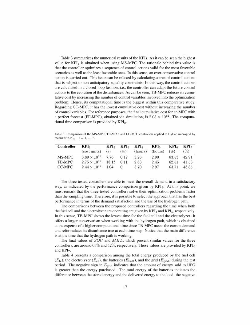
Table 3 summarizes the numerical results of the KPIs. As it can be seen the highestvalue for KPI1 is obtained when using MS-MPC. The rationale behind this value isthat the controller optimizes a sequence of control actions valid for the most favorablescenarios as well as the least favorable ones. In this sense, an over-conservative controlaction is carried out. This issue can be relaxed by calculating a tree of control actionsthat is subject to non-anticipatory equality constraints. In this way, the control actionsare calculated in a closed-loop fashion, i.e., the controller can adapt the future controlactions to the evolution of the disturbances. As can be seen, TB-MPC reduces its cumu-lative cost by increasing the number of control variables involved into the optimizationproblem. Hence, its computational time is the biggest within this comparative study.Regarding CC-MPC, it has the lowest cumulative cost without increasing the numberof control variables. For reference purposes, the final cumulative cost for an MPC witha perfect forecast (PF-MPC), obtained via simulation, is 2.05 × 10¹². The computa-tional time comparison is provided by KPI2.
Table 3: Comparison of the MS-MPC, TB-MPC, and CC-MPC controllers applied to HyLab microgrid bymeans of KPIi, i = 1, ..., 7.
Controller KPI1 KPI2 KPI3 KPI4 KPI5 KPI6 KPI7(cost units) (s) (%) (hours) (hours) (%) (%)
MS-MPC 3.89× 10¹² 7.76 0.12 3.26 2.90 63.53 42.91TB-MPC 2.75× 10¹² 18.15 0.11 2.63 2.45 62.51 41.58CC-MPC 2.44× 10¹² 1.04 0 3.70 2.97 63.71 43.85
The three tested controllers are able to meet the overall demand in a satisfactoryway, as indicated by the performance comparison given by KPI3. At this point, wemust remark that the three tested controllers solve their optimization problems fasterthan the sampling time. Therefore, it is possible to select the approach that has the bestperformance in terms of the demand satisfaction and the use of the hydrogen path.
The comparisons between the proposed controllers regarding the time when boththe fuel cell and the electrolyzer are operating are given by KPI4 and KPI5, respectively.In this sense, TB-MPC shows the lowest time for the fuel cell and the electrolyzer. Itoffers a larger conservatism when working with the hydrogen path, which is obtainedat the expense of a higher computational time since TB-MPC meets the current demandand reformulates its disturbance tree at each time step. Notice that the main differenceis at the time that the hydrogen path is working.
The final values of SOC and MHL, which present similar values for the threecontrollers, are around 63% and 42%, respectively. These values are provided by KPI6and KPI7.
Table 4 presents a comparison among the total energy produced by the fuel cell(Efc), the electrolyzer (Eez), the batteries (Ebatt), and the grid (Egrid) during the testperiod. The negative sign in Egrid indicates that the amount of energy sold to UPGis greater than the energy purchased. The total energy of the batteries indicates thedifference between the stored energy and the delivered energy to the load: the negative
17
value means that the stored energy predominates over the delivered energy.
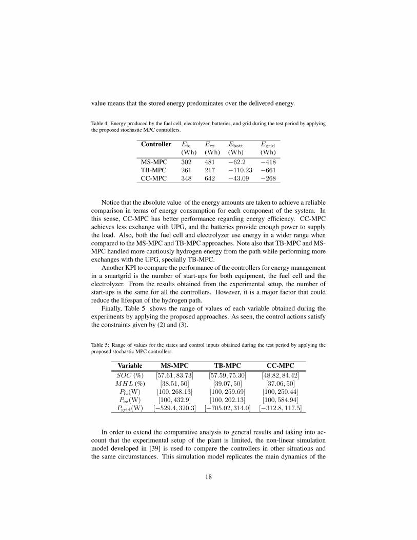
Table 4: Energy produced by the fuel cell, electrolyzer, batteries, and grid during the test period by applyingthe proposed stochastic MPC controllers.
Controller Efc Eez Ebatt Egrid
(Wh) (Wh) (Wh) (Wh)MS-MPC 302 481 −62.2 −418TB-MPC 261 217 −110.23 −661CC-MPC 348 642 −43.09 −268
Notice that the absolute value of the energy amounts are taken to achieve a reliablecomparison in terms of energy consumption for each component of the system. Inthis sense, CC-MPC has better performance regarding energy efficiency. CC-MPCachieves less exchange with UPG, and the batteries provide enough power to supplythe load. Also, both the fuel cell and electrolyzer use energy in a wider range whencompared to the MS-MPC and TB-MPC approaches. Note also that TB-MPC and MS-MPC handled more cautiously hydrogen energy from the path while performing moreexchanges with the UPG, specially TB-MPC.
Another KPI to compare the performance of the controllers for energy managementin a smartgrid is the number of start-ups for both equipment, the fuel cell and theelectrolyzer. From the results obtained from the experimental setup, the number ofstart-ups is the same for all the controllers. However, it is a major factor that couldreduce the lifespan of the hydrogen path.
Finally, Table 5 shows the range of values of each variable obtained during theexperiments by applying the proposed approaches. As seen, the control actions satisfythe constraints given by (2) and (3).
Table 5: Range of values for the states and control inputs obtained during the test period by applying theproposed stochastic MPC controllers.
Variable MS-MPC TB-MPC CC-MPCSOC (%) [57.61, 83.73] [57.59, 75.30] [48.82, 84.42]MHL (%) [38.51, 50] [39.07, 50] [37.06, 50]Pfc(W) [100, 268.13] [100, 259.69] [100, 250.44]Pez(W) [100, 432.9] [100, 202.13] [100, 584.94]Pgrid(W) [−529.4, 320.3] [−705.02, 314.0] [−312.8, 117.5]
In order to extend the comparative analysis to general results and taking into ac-count that the experimental setup of the plant is limited, the non-linear simulationmodel developed in [39] is used to compare the controllers in other situations andthe same circumstances. This simulation model replicates the main dynamics of the
18
real plant with enough accuracy. An additional case study for testing the three stochas-tic MPC controllers and a PF-MPC controller is introduced to enhance the results andobtain conclusions.
Figure 5 shows the evolution of the signals by applying the three stochastic MPCcontrollers and a PF-MPC controller for a cloudy day in the simulation model of theHyLab microgrid. All controllers present the same evolution to satisfy the demand.The fuel cells are turned on when the power from the renewable sources is not enoughto meet the electric demand. Hence, SOC and MHL decrease gradually to supplypower to the load. For this particular day, the microgrid imports energy power fromthe UPG. Given that the excess of renewable energy production over the demand is notenough, the batteries are charged, and the electrolyzer stays off.
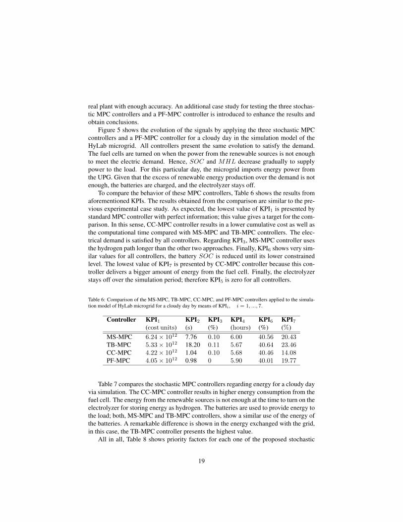
To compare the behavior of these MPC controllers, Table 6 shows the results fromaforementioned KPIs. The results obtained from the comparison are similar to the pre-vious experimental case study. As expected, the lowest value of KPI1 is presented bystandard MPC controller with perfect information; this value gives a target for the com-parison. In this sense, CC-MPC controller results in a lower cumulative cost as well asthe computational time compared with MS-MPC and TB-MPC controllers. The elec-trical demand is satisfied by all controllers. Regarding KPI3, MS-MPC controller usesthe hydrogen path longer than the other two approaches. Finally, KPI6 shows very sim-ilar values for all controllers, the battery SOC is reduced until its lower constrainedlevel. The lowest value of KPI7 is presented by CC-MPC controller because this con-troller delivers a bigger amount of energy from the fuel cell. Finally, the electrolyzerstays off over the simulation period; therefore KPI5 is zero for all controllers.
Table 6: Comparison of the MS-MPC, TB-MPC, CC-MPC, and PF-MPC controllers applied to the simula-tion model of HyLab microgrid for a cloudy day by means of KPIi, i = 1, ..., 7.
Controller KPI1 KPI2 KPI3 KPI4 KPI6 KPI7(cost units) (s) (%) (hours) (%) (%)
MS-MPC 6.24× 10¹² 7.76 0.10 6.00 40.56 20.43TB-MPC 5.33× 10¹² 18.20 0.11 5.67 40.64 23.46CC-MPC 4.22× 10¹² 1.04 0.10 5.68 40.46 14.08PF-MPC 4.05× 10¹² 0.98 0 5.90 40.01 19.77
Table 7 compares the stochastic MPC controllers regarding energy for a cloudy dayvia simulation. The CC-MPC controller results in higher energy consumption from thefuel cell. The energy from the renewable sources is not enough at the time to turn on theelectrolyzer for storing energy as hydrogen. The batteries are used to provide energy tothe load; both, MS-MPC and TB-MPC controllers, show a similar use of the energy ofthe batteries. A remarkable difference is shown in the energy exchanged with the grid,in this case, the TB-MPC controller presents the highest value.
All in all, Table 8 shows priority factors for each one of the proposed stochastic
19
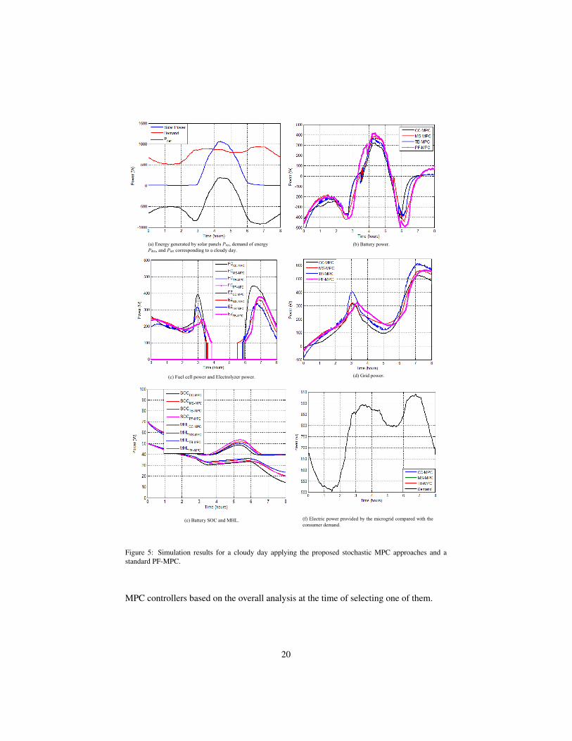
(a) Energy generated by solar panels Pres, demand of energy
Pden, and Pnet corresponding to a cloudy day.
(b) Battery power.
(c) Fuel cell power and Electrolyzer power.
(e) Battery SOC and MHL. (f) Electric power provided by the microgrid compared with the
consumer demand.
(d) Grid power.
Figure 5: Simulation results for a cloudy day applying the proposed stochastic MPC approaches and astandard PF-MPC.
MPC controllers based on the overall analysis at the time of selecting one of them.
20
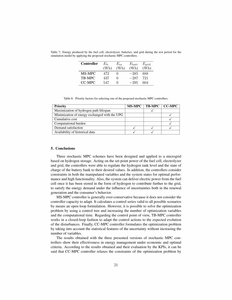
Table 7: Energy produced by the fuel cell, electrolyzer, batteries, and grid during the test period for thesimulation model by applying the proposed stochastic MPC controllers.
Controller Efc Eez Ebatt Egrid
(Wh) (Wh) (Wh) (Wh)MS-MPC 472 0 −285 688TB-MPC 437 0 −287 721CC-MPC 547 0 −295 604
Table 8: Priority factors for selecting one of the proposed stochastic MPC controllers.
Priority MS-MPC TB-MPC CC-MPCMaximization of hydrogen path lifespan XMinimization of energy exchanged with the UPG XCumulative cost XComputational burden XDemand satisfaction X X XAvailability of historical data X X
5. Conclusions
Three stochastic MPC schemes have been designed and applied to a microgridbased on hydrogen storage. Acting on the set-point power of the fuel cell, electrolyzerand grid, the controllers were able to regulate the hydrogen tank level and the state ofcharge of the battery bank to their desired values. In addition, the controllers considerconstraints in both the manipulated variables and the system states for optimal perfor-mance and high functionality. Also, the system can deliver electric power from the fuelcell once it has been stored in the form of hydrogen to contribute further to the grid,to satisfy the energy demand under the influence of uncertainties both in the renewalgeneration and the consumer’s behavior.
MS-MPC controller is generally over-conservative because it does not consider thecontroller capacity to adapt. It calculates a control series valid to all possible scenariosby means an open-loop formulation. However, it is possible to solve the optimizationproblem by using a control tree and increasing the number of optimization variablesand the computational time. Regarding the control point of view, TB-MPC controllerworks in a closed-loop fashion to adapt the control actions to the expected evolutionof the disturbances. Finally, CC-MPC controller formulates the optimization problemby taking into account the statistical features of the uncertainty without increasing thenumber of variables.
The results obtained with the three presented versions of stochastic MPC con-trollers show their effectiveness in energy management under economic and optimalcriteria. According to the results obtained and their evaluation by the KPIs, it can besaid that CC-MPC controller relaxes the constraints of the optimization problem by
21
assuming a risk to offer better performance, resulting in a lower cost, less energy ex-change with the network when compared to MS-MPC and TB-MPC controllers. Thisis also the approach with the lowest computational burden. The downside of this ap-proach is that it requires a statical characterization of the disturbances.
The TB-MPC approach, according to the results, provides a more moderate use ofthe hydrogen path, which could lead to a longer equipment lifespan. From the point ofview of the user, the energy demand is fulfilled by increasing energy exchange with thenetwork.
The MS-MPC approach provides a certain robustness of the system, generatingcontrol actions able to cope with potential disturbances. This approach provides atrade-off between the time of use of the equipment and the satisfaction of the energydemand.
Other factors that are important to take into account are the initial conditions forSOC and MHL. These values will determine the evolution of the variables. Besides,the final value of these variables will take an additional meaning of comparison after alonger time of use of the plant. However, they have been employed in a smaller periodto show how they finish after the experiments.
Acknowledgement
Financial support from the Spanish Ministry of Economy and Competitiveness(COOPERA project, under grant DPI2013-46912-C2-1-R) and the project ECOCIS(Ref. DPI2013-482443-C2-1-R) is acknowledged.
References
[1] J. P. Lopes, C. Moreira, A. Madureira, Defining control strategies for microgridsislanded operation, IEEE Transactions on Power Systems 21 (2) (2006) 916–924.
[2] L. Valverde, C. Bordons, F. Rosa, Integration of fuel cell technologies inrenewable-energy-based microgrids optimizing operational costs and durability,IEEE Transactions on Industrial Electronics 63 (1) (2016) 167–177.
[3] C. Kunusch, C. Ocampo-Martinez, M. Valla, Modeling, diagnosis, and control offuel-cell-based technologies and their integration in smart grids and automotivesystems, IEEE Transactions on Industrial Electronics 62 (8) (2015) 5143–5145.
[4] L. Valverde, F. Rosa, C. Bordons, Design, planning and management of ahydrogen-based microgrid, IEEE Transactions on Industrial Informatics 9 (3)(2013) 1398–1404.
[5] D. Recio, C. Ocampo-Martinez, M. Serra, Design of linear predictive controllersapplied to ethanol steam reformers for hydrogen production, International Journalof Hydrogen Energy 37(15) (2012) 11141–11156.
[6] T. Dragicevic, J. Guerrero, J. Vasquez, A distributed control strategy for coordi-nation of an autonomous LVDC microgrid based on power-line signaling, IEEETransactions on Industrial Electronics 61 (7) (2014) 3313–3326.
22
[7] E. F. Camacho, C. Bordons, Model Predictive Control. Second Edition, Springer-Verlag, London, England, 2004.
[8] F. Garcia-Torres, C. Bordons, Optimal economical schedule of hydrogen-basedmicrogrids with hybrid storage using model predictive control, IEEE Transactionson Industrial Electronics 62 (8) (2015) 5195–5207.
[9] M. Pereira, D. Limon, D. Munoz de la Pena, L. Valverde, T. Alamo, Periodiceconomic control of a nonisolated microgrid, IEEE Transactions on IndustrialElectronics 62 (8) (2015) 5247–5255.
[10] G. Bruni, S. Cordiner, V. Mulone, V. Rocco, F. Spagnolo, A study on the energymanagement in domestic micro-grids based on model predictive control strate-gies, Energy Conversion and Management 102 (2015) 50–58.
[11] A. Parisio, E. Rikos, G. Tzamalis, L. Glielmo, Use of model predictive controlfor experimental microgrid optimization, Applied Energy 115 (2014) 37–46.
[12] J. Patino, A. Marquez, J. Espinosa, An economic MPC approach for a microgridenergy management system, in: Proceedings of the Transmission DistributionConference and Exposition - Latin America (PES T D-LA), IEEE PES, Medellın,Colombia, 2014, pp. 1–6.
[13] P. O. Kriett, M. Salani, Optimal control of a residential microgrid, Energy 42 (1)(2012) 321–330.
[14] D. E. Olivares, A. Mehrizi-Sani, A. H. Etemadi, C. A. Canizares, R. Iravani,M. Kazerani, A. H. Hajimiragha, O. Gomis-Bellmunt, M. Saeedifard, R. Palma-Behnke, G. Jimenez-Estevez, N. Hatziargyriou, Trends in microgrid control,IEEE Transactions on Smart Grid 5 (4) (2014) 1905–1919.
[15] L. I. Minchala-Avila, L. E. Garza-Castanon, A. Vargas-Martınez, Y. Zhang, A re-view of optimal control techniques applied to the energy management and controlof microgrids, Procedia Computer Science 52 (2015) 780 – 787.
[16] D. Bernardini, A. Bemporad, Scenario-based model predictive control of stochas-tic constrained linear systems, Joint 48th IEEE Conference on Decision and Con-trol and 28th Chinese Control Conference, Shanghai, P.R. China (2009) 6333–6338.
[17] C. A. Hans, V. Nenchev, J. Raisch, C. Reincke-Collon, A. Younicos, Min-maxmodel predictive operation control of microgrids, in: Proceedings of the 19thIFAC World Congress, Cape Town, South Africa, 2014, pp. 10287–10292.
[18] D. Munoz de la Pena, A. Bemporad, T. Alamo, Stochastic programming appliedto model predictive control, in: Proceedings of the 44th IEEE Conference onDecision and Control, and European Control Conference (CDC-ECC), Seville,Spain, 2005, pp. 1361–1366.
23
[19] P. J. van Overloop, S. Weijs, S. Dijkstra, Multiple model predictive control on adrainage canal system, Control Engineering Practice 16 (5) (2008) 531–540.
[20] D. E. Olivares, J. D. Lara, C. A. Canizares, M. Kazerani, Stochastic-predictiveenergy management system for isolated microgrids, IEEE Transactions on SmartGrid 6 (6) (2015) 2681–2693.
[21] T. Niknam, R. Azizipanah-Abarghooee, M. R. Narimani, An efficient scenario-based stochastic programming framework for multi-objective optimal micro-gridoperation, Applied Energy 99 (2012) 455 – 470.
[22] G. Calafiore, M. Campi, The scenario approach to robust control design, IEEETransactions on Automatic Control 51 (5) (2006) 742–753.
[23] S. Lucia, T. Finkler, D. Basak, S. Engell, A new robust NMPC scheme and itsapplication to a semi-batch reactor example., In Proc. of the International Sym-posium on Advanced Control of Chemical Processes, Singapore (2012) 69–74.
[24] M. Petrollese, L. Valverde, D. Cocco, G. Cau, J. Guerra, Real-time integration ofoptimal generation scheduling with mpc for the energy management of a renew-able hydrogen-based microgrid, Applied Energy 166 (2016) 96–106.
[25] J. M. Maestre, L. Raso, P. J. Van Overloop, B. De Schutter, Distributed tree-based model predictive control on an open water system, in: Proceedings of theAmerican Control Conference (ACC), Montreal, Canada, 2012, pp. 1985–1990.
[26] Q. Wang, Y. Guan, J. Wang, A chance-constrained two-stage stochastic programfor unit commitment with uncertain wind power output, IEEE Transactions onPower Systems 27 (1) (2012) 206–215.
[27] M. Ono, U. Topcu, M. Yo, S. Adachi, Risk-limiting power grid control with anarma-based prediction model, in: Proceedings of the 52nd IEEE Annual Confer-ence on Decision and Control (CDC), Florence, Italy, 2013, pp. 4949–4956.
[28] J. Grosso, C. Ocampo-Martinez, V. Puig, B. Joseph, Chance-constrained modelpredictive control for drinking water networks, Journal of Process Control 24 (5)(2014) 504–516.
[29] J. M. Grosso, P. Velarde, C. Ocampo-Martinez, J. M. Maestre, V. Puig, Stochasticmodel predictive control approaches applied to drinking water networks, OptimalControl Applications and Methods In Press. doi:10.1002/oca.2269.
[30] A. Hooshmand, B. Asghari, R. Sharma, A novel cost-aware multi-objective en-ergy management method for microgrids, in: Proceedings of the Innovative SmartGrid Technologies (ISGT), IEEE PES, Washington, DC, USA, 2013, pp. 1–6.
[31] Z. Yu, L. McLaughlin, L. Jia, M. C. Murphy-Hoye, A. Pratt, L. Tong, Modelingand stochastic control for home energy management, in: Proceedings of the IEEEPower and Energy Society General Meeting, San Diego, California, USA, 2012,pp. 1–9.
24
[32] P. Meibom, R. Barth, B. Hasche, H. Brand, C. Weber, M. O’Malley, Stochasticoptimization model to study the operational impacts of high wind penetrations inIreland, IEEE Transactions on Power Systems 26 (3) (2011) 1367–1379.
[33] T. Hovgaard, L. Larsen, J. Jorgensen, Robust economic MPC for a power manage-ment scenario with uncertainties, in: Proceedings of the 50th IEEE Conference onDecision and Control and European Control Conference (CDC-ECC), Orlando,Florida, 2011, pp. 1515–1520.
[34] L. Valverde, F. Rosa, A. del Real, A. Arce, C. Bordons, Modeling, simulation andexperimental set-up of a renewable hydrogen-based domestic microgrid, Interna-tional Journal of Hydrogen Energy 38 (2013) 11672–11684.
[35] C. Bordons, F. Garcıa-Torres, L. Valverde, Optimal energy management for re-newable energy microgrids (in Spanish), Revista Iberoamericana de Automaticae Informatica Industrial RIAI 12 (2) (2015) 117–132.
[36] B. S. Lee, H. Y. Park, I. Choi, M. K. Cho, H. J. Kim, S. J. Yoo, D. Henkensmeier,J. Y. Kim, S. W. Nam, S. Park, et al., Polarization characteristics of a low cata-lyst loading pem water electrolyzer operating at elevated temperature, Journal ofPower Sources 309 (2016) 127–134.
[37] A. J. Del Real, A. Arce, C. Bordons, Development and experimental validationof a pem fuel cell dynamic model, Journal of Power Sources 173 (1) (2007) 310–324.
[38] M. Tanrioven, M. Alam, Reliability modeling and assessment of grid-connectedpem fuel cell power plants, Journal of Power Sources 142 (1) (2005) 264–278.
[39] L. Valverde, F. Rosa, A. del Real, A. Arce, C. Bordons, Modeling, simulation andexperimental set-up of a renewable hydrogen-based domestic microgrid, Interna-tional Journal of Hydrogen Energy 38 (27) (2013) 11672–11684.
[40] G. Schildbach, L. Fagiano, C. Frei, M. Morari, The scenario approach for stochas-tic model predictive control with bounds on closed-loop constraint violations,Automatica 50 (12) (2014) 3009–3018.
[41] L. Giulioni, Stochastic model predictive control with application to distributedcontrol systems, Ph.D. thesis, Politecnico di Milano (2015).
[42] L. Raso, N. Giesen, P. Stive, D. Schwanenberg, P. Overloop, Tree structure gener-ation from ensemble forecasts for real time control, Hydrological Processes 27 (1)(2013) 75–82.
[43] L. Raso, D. Schwanenberg, N. van de Giesen, P. van Overloop, Short-term op-timal operation of water systems using ensemble forecasts, Advances in WaterResources 71 (2014) 200 – 208.
[44] A. Brooke, D. Kendrick, A. Meeraus, R. Raman, General algebraic modelingsystem (GAMS): A users guide, Boyd & Fraser publishing company, Danvers,Massachusetts.
25

[45] E. Karfopoulos, L. Tena, A. Torres, P. Salas, J. G. Jorda, A. Dimeas, N. Hatziar-gyriou, A multi-agent system providing demand response services from residen-tial consumers, Electric Power Systems Research 120 (2015) 163 – 176.
26