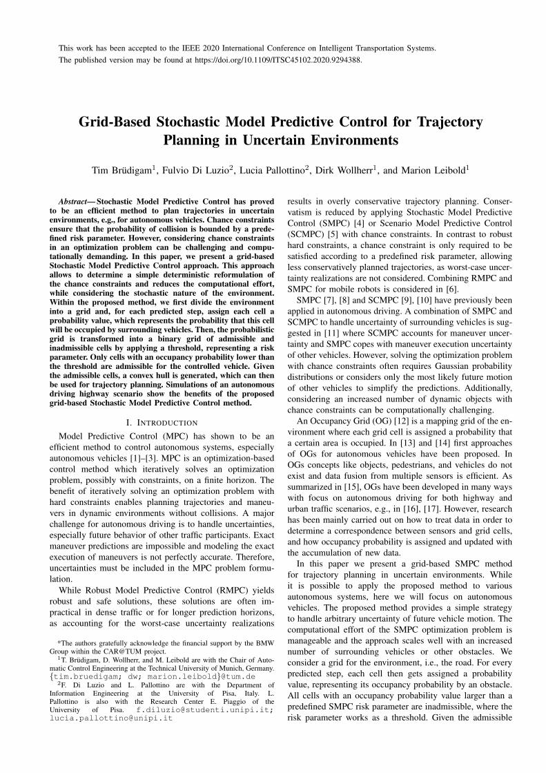
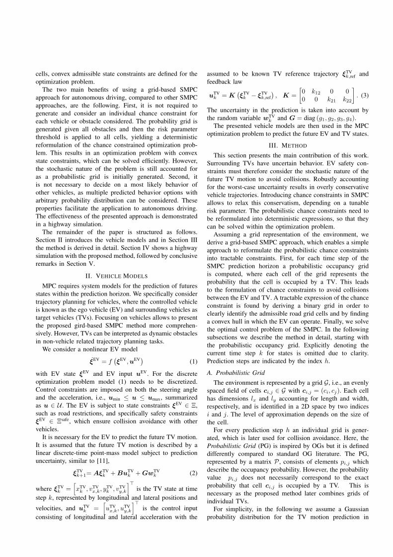
Grid-Based Stochastic Model Predictive Control for TrajectoryPlanning in Uncertain Environments

Tim Brudigam1, Fulvio Di Luzio2, Lucia Pallottino2, Dirk Wollherr1, and Marion Leibold1

Abstract— Stochastic Model Predictive Control has provedto be an efficient method to plan trajectories in uncertainenvironments, e.g., for autonomous vehicles. Chance constraintsensure that the probability of collision is bounded by a prede-fined risk parameter. However, considering chance constraintsin an optimization problem can be challenging and compu-tationally demanding. In this paper, we present a grid-basedStochastic Model Predictive Control approach. This approachallows to determine a simple deterministic reformulation ofthe chance constraints and reduces the computational effort,while considering the stochastic nature of the environment.Within the proposed method, we first divide the environmentinto a grid and, for each predicted step, assign each cell aprobability value, which represents the probability that this cellwill be occupied by surrounding vehicles. Then, the probabilisticgrid is transformed into a binary grid of admissible andinadmissible cells by applying a threshold, representing a riskparameter. Only cells with an occupancy probability lower thanthe threshold are admissible for the controlled vehicle. Giventhe admissible cells, a convex hull is generated, which can thenbe used for trajectory planning. Simulations of an autonomousdriving highway scenario show the benefits of the proposedgrid-based Stochastic Model Predictive Control method.

I. INTRODUCTION

This work has been accepted to the IEEE 2020 International Conference on Intelligent Transportation Systems.The published version may be found at https://doi.org/10.1109/ITSC45102.2020.9294388.

Model Predictive Control (MPC) has shown to be anefficient method to control autonomous systems, especiallyautonomous vehicles [1]–[3]. MPC is an optimization-basedcontrol method which iteratively solves an optimizationproblem, possibly with constraints, on a finite horizon. Thebenefit of iteratively solving an optimization problem withhard constraints enables planning trajectories and maneu-vers in dynamic environments without collisions. A majorchallenge for autonomous driving is to handle uncertainties,especially future behavior of other traffic participants. Exactmaneuver predictions are impossible and modeling the exactexecution of maneuvers is not perfectly accurate. Therefore,uncertainties must be included in the MPC problem formu-lation.

While Robust Model Predictive Control (RMPC) yieldsrobust and safe solutions, these solutions are often im-practical in dense traffic or for longer prediction horizons,as accounting for the worst-case uncertainty realizations

*The authors gratefully acknowledge the financial support by the BMWGroup within the CAR@TUM project.

1T. Brudigam, D. Wollherr, and M. Leibold are with the Chair of Auto-matic Control Engineering at the Technical University of Munich, Germany.{tim.bruedigam; dw; marion.leibold}@tum.de

2F. Di Luzio and L. Pallottino are with the Department ofInformation Engineering at the University of Pisa, Italy. L.Pallottino is also with the Research Center E. Piaggio of theUniversity of Pisa. f.diluzio@studenti.unipi.it;lucia.pallottino@unipi.it

results in overly conservative trajectory planning. Conser-vatism is reduced by applying Stochastic Model PredictiveControl (SMPC) [4] or Scenario Model Predictive Control(SCMPC) [5] with chance constraints. In contrast to robusthard constraints, a chance constraint is only required to besatisfied according to a predefined risk parameter, allowingless conservatively planned trajectories, as worst-case uncer-tainty realizations are not considered. Combining RMPC andSMPC for mobile robots is considered in [6].

SMPC [7], [8] and SCMPC [9], [10] have previously beenapplied in autonomous driving. A combination of SMPC andSCMPC to handle uncertainty of surrounding vehicles is sug-gested in [11] where SCMPC accounts for maneuver uncer-tainty and SMPC copes with maneuver execution uncertaintyof other vehicles. However, solving the optimization problemwith chance constraints often requires Gaussian probabilitydistributions or considers only the most likely future motionof other vehicles to simplify the predictions. Additionally,considering an increased number of dynamic objects withchance constraints can be computationally challenging.

An Occupancy Grid (OG) [12] is a mapping grid of the en-vironment where each grid cell is assigned a probability thata certain area is occupied. In [13] and [14] first approachesof OGs for autonomous vehicles have been proposed. InOGs concepts like objects, pedestrians, and vehicles do notexist and data fusion from multiple sensors is efficient. Assummarized in [15], OGs have been developed in many wayswith focus on autonomous driving for both highway andurban traffic scenarios, e.g., in [16], [17]. However, researchhas been mainly carried out on how to treat data in order todetermine a correspondence between sensors and grid cells,and how occupancy probability is assigned and updated withthe accumulation of new data.

In this paper we present a grid-based SMPC methodfor trajectory planning in uncertain environments. Whileit is possible to apply the proposed method to variousautonomous systems, here we will focus on autonomousvehicles. The proposed method provides a simple strategyto handle arbitrary uncertainty of future vehicle motion. Thecomputational effort of the SMPC optimization problem ismanageable and the approach scales well with an increasednumber of surrounding vehicles or other obstacles. Weconsider a grid for the environment, i.e., the road. For everypredicted step, each cell then gets assigned a probabilityvalue, representing its occupancy probability by an obstacle.All cells with an occupancy probability value larger than apredefined SMPC risk parameter are inadmissible, where therisk parameter works as a threshold. Given the admissible

cells, convex admissible state constraints are defined for theoptimization problem.

The two main benefits of using a grid-based SMPCapproach for autonomous driving, compared to other SMPCapproaches, are the following. First, it is not required togenerate and consider an individual chance constraint foreach vehicle or obstacle considered. The probability grid isgenerated given all obstacles and then the risk parameterthreshold is applied to all cells, yielding a deterministicreformulation of the chance constrained optimization prob-lem. This results in an optimization problem with convexstate constraints, which can be solved efficiently. However,the stochastic nature of the problem is still accounted foras a probabilistic grid is initially generated. Second, itis not necessary to decide on a most likely behavior ofother vehicles, as multiple predicted behavior options witharbitrary probability distribution can be considered. Theseproperties facilitate the application to autonomous driving.The effectiveness of the presented approach is demonstratedin a highway simulation.

The remainder of the paper is structured as follows.Section II introduces the vehicle models and in Section IIIthe method is derived in detail. Section IV shows a highwaysimulation with the proposed method, followed by conclusiveremarks in Section V.

II. VEHICLE MODELS

MPC requires system models for the prediction of futuresstates within the prediction horizon. We specifically considertrajectory planning for vehicles, where the controlled vehicleis known as the ego vehicle (EV) and surrounding vehicles astarget vehicles (TVs). Focusing on vehicles allows to presentthe proposed gird-based SMPC method more comprehen-sively. However, TVs can be interpreted as dynamic obstaclesin non-vehicle related trajectory planning tasks.

We consider a nonlinear EV model

ξEV = f(ξEV,uEV) (1)

with EV state ξEV and EV input uEV. For the discreteoptimization problem model (1) needs to be discretized.Control constraints are imposed on both the steering angleand the acceleration, i.e., umin ≤ u ≤ umax, summarizedas u ∈ U . The EV is subject to state constraints ξEV ∈ Ξ,such as road restrictions, and specifically safety constraintsξEV ∈ Ξsafe, which ensure collision avoidance with othervehicles.

It is necessary for the EV to predict the future TV motion.It is assumed that the future TV motion is described by alinear discrete-time point-mass model subject to predictionuncertainty, similar to [11],

ξTVk+1= AξTV

k +BuTVk +GwTV

k (2)

where ξTVk =

[xTVk , vTV

x,k, yTVk , vTV

y,k

]>is the TV state at time

step k, represented by longitudinal and lateral positions and

velocities, and uTVk =

[uTVx,k, u

TVy,k

]>is the control input

consisting of longitudinal and lateral acceleration with the

assumed to be known TV reference trajectory ξTVk,ref and

feedback law

uTVk = K

(ξTVk − ξTV

k,ref

), K =

[0 k12 0 00 0 k21 k22

]. (3)

The uncertainty in the prediction is taken into account bythe random variable wTV

k and G = diag (g1, g2, g3, g4).The presented vehicle models are then used in the MPC

optimization problem to predict the future EV and TV states.

III. METHOD

This section presents the main contribution of this work.Surrounding TVs have uncertain behavior. EV safety con-straints must therefore consider the stochastic nature of thefuture TV motion to avoid collisions. Robustly accountingfor the worst-case uncertainty results in overly conservativevehicle trajectories. Introducing chance constraints in SMPCallows to relax this conservatism, depending on a tunablerisk parameter. The probabilistic chance constraints need tobe reformulated into deterministic expressions, so that theycan be solved within the optimization problem.

Assuming a grid representation of the environment, wederive a grid-based SMPC approach, which enables a simpleapproach to reformulate the probabilistic chance constraintsinto tractable constraints. First, for each time step of theSMPC prediction horizon a probabilistic occupancy gridis computed, where each cell of the grid represents theprobability that the cell is occupied by a TV. This leadsto the formulation of chance constraints to avoid collisionsbetween the EV and TV. A tractable expression of the chanceconstraint is found by deriving a binary grid in order toclearly identify the admissible road grid cells and by findinga convex hull in which the EV can operate. Finally, we solvethe optimal control problem of the SMPC. In the followingsubsections we describe the method in detail, starting withthe probabilistic occupancy grid. Explicitly denoting thecurrent time step k for states is omitted due to clarity.Prediction steps are indicated by the index h.

A. Probabilistic Grid

The environment is represented by a grid G, i.e., an evenlyspaced field of cells ci,j ∈ G with ci,j = (ci, cj). Each cellhas dimensions lx and ly accounting for length and width,respectively, and is identified in a 2D space by two indicesi and j. The level of approximation depends on the size ofthe cell.

For every prediction step h an individual grid is gener-ated, which is later used for collision avoidance. Here, theProbabilistic Grid (PG) is inspired by OGs but it is defineddifferently compared to standard OG literature. The PG,represented by a matrix P , consists of elements pi,j whichdescribe the occupancy probability. However, the probabilityvalue pi,j does not necessarily correspond to the exactprobability that cell ci,j is occupied by a TV. This isnecessary as the proposed method later combines grids ofindividual TVs.

For simplicity, in the following we assume a Gaussianprobability distribution for the TV motion prediction in

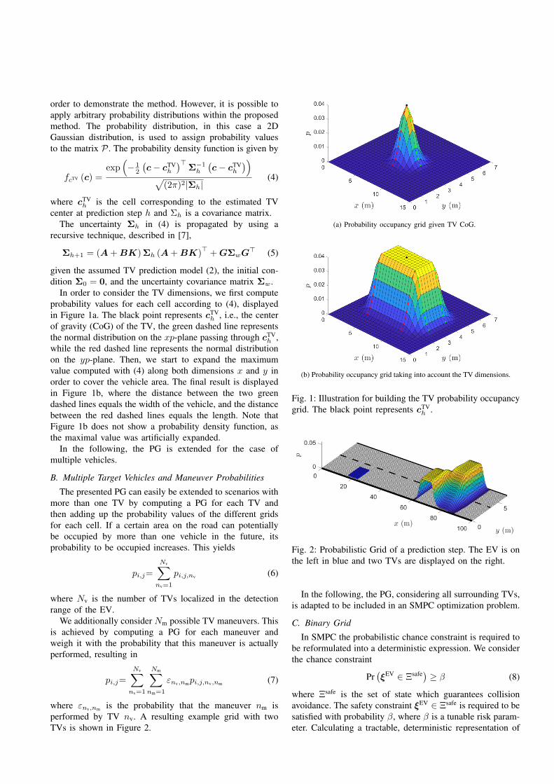
order to demonstrate the method. However, it is possible toapply arbitrary probability distributions within the proposedmethod. The probability distribution, in this case a 2DGaussian distribution, is used to assign probability valuesto the matrix P . The probability density function is given by

fcTV (c) =exp

(− 1

2

(c− cTV

h

)>Σ−1h

(c− cTV

h

))√(2π)2|Σh|

(4)

where cTVh is the cell corresponding to the estimated TV

center at prediction step h and Σh is a covariance matrix.The uncertainty Σh in (4) is propagated by using a

recursive technique, described in [7],

Σh+1 = (A+BK) Σh (A+BK)>

+GΣwG> (5)

given the assumed TV prediction model (2), the initial con-dition Σ0 = 0, and the uncertainty covariance matrix Σw.

In order to consider the TV dimensions, we first computeprobability values for each cell according to (4), displayedin Figure 1a. The black point represents cTV

h , i.e., the centerof gravity (CoG) of the TV, the green dashed line representsthe normal distribution on the xp-plane passing through cTV

h ,while the red dashed line represents the normal distributionon the yp-plane. Then, we start to expand the maximumvalue computed with (4) along both dimensions x and y inorder to cover the vehicle area. The final result is displayedin Figure 1b, where the distance between the two greendashed lines equals the width of the vehicle, and the distancebetween the red dashed lines equals the length. Note thatFigure 1b does not show a probability density function, asthe maximal value was artificially expanded.

In the following, the PG is extended for the case ofmultiple vehicles.

B. Multiple Target Vehicles and Maneuver Probabilities

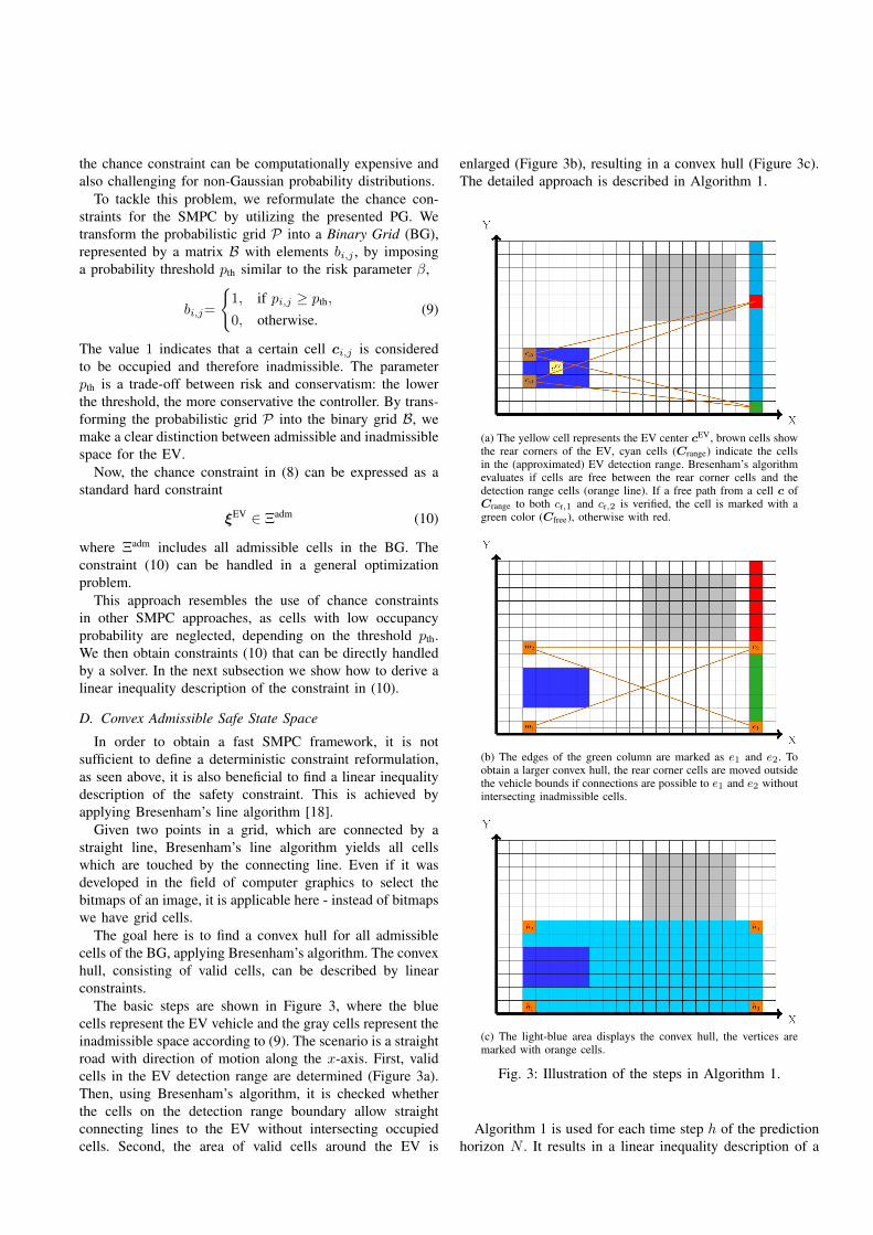
The presented PG can easily be extended to scenarios withmore than one TV by computing a PG for each TV andthen adding up the probability values of the different gridsfor each cell. If a certain area on the road can potentiallybe occupied by more than one vehicle in the future, itsprobability to be occupied increases. This yields

pi,j=

Nv∑nv=1

pi,j,nv (6)

where Nv is the number of TVs localized in the detectionrange of the EV.

We additionally consider Nm possible TV maneuvers. Thisis achieved by computing a PG for each maneuver andweigh it with the probability that this maneuver is actuallyperformed, resulting in

pi,j=

Nv∑nv=1

Nm∑nm=1

εnv,nmpi,j,nv,nm (7)

where εnv,nm is the probability that the maneuver nm isperformed by TV nv. A resulting example grid with twoTVs is shown in Figure 2.

(a) Probability occupancy grid given TV CoG.

(b) Probability occupancy grid taking into account the TV dimensions.

Fig. 1: Illustration for building the TV probability occupancygrid. The black point represents cTV

h .

Fig. 2: Probabilistic Grid of a prediction step. The EV is onthe left in blue and two TVs are displayed on the right.

In the following, the PG, considering all surrounding TVs,is adapted to be included in an SMPC optimization problem.

C. Binary Grid

In SMPC the probabilistic chance constraint is required tobe reformulated into a deterministic expression. We considerthe chance constraint

Pr(ξEV ∈ Ξsafe) ≥ β (8)

where Ξsafe is the set of state which guarantees collisionavoidance. The safety constraint ξEV ∈ Ξsafe is required to besatisfied with probability β, where β is a tunable risk param-eter. Calculating a tractable, deterministic representation of

the chance constraint can be computationally expensive andalso challenging for non-Gaussian probability distributions.

To tackle this problem, we reformulate the chance con-straints for the SMPC by utilizing the presented PG. Wetransform the probabilistic grid P into a Binary Grid (BG),represented by a matrix B with elements bi,j , by imposinga probability threshold pth similar to the risk parameter β,

bi,j=

{1, if pi,j ≥ pth,

0, otherwise.(9)

The value 1 indicates that a certain cell ci,j is consideredto be occupied and therefore inadmissible. The parameterpth is a trade-off between risk and conservatism: the lowerthe threshold, the more conservative the controller. By trans-forming the probabilistic grid P into the binary grid B, wemake a clear distinction between admissible and inadmissiblespace for the EV.

Now, the chance constraint in (8) can be expressed as astandard hard constraint

ξEV ∈ Ξadm (10)

where Ξadm includes all admissible cells in the BG. Theconstraint (10) can be handled in a general optimizationproblem.

This approach resembles the use of chance constraintsin other SMPC approaches, as cells with low occupancyprobability are neglected, depending on the threshold pth.We then obtain constraints (10) that can be directly handledby a solver. In the next subsection we show how to derive alinear inequality description of the constraint in (10).

D. Convex Admissible Safe State Space

In order to obtain a fast SMPC framework, it is notsufficient to define a deterministic constraint reformulation,as seen above, it is also beneficial to find a linear inequalitydescription of the safety constraint. This is achieved byapplying Bresenham’s line algorithm [18].

Given two points in a grid, which are connected by astraight line, Bresenham’s line algorithm yields all cellswhich are touched by the connecting line. Even if it wasdeveloped in the field of computer graphics to select thebitmaps of an image, it is applicable here - instead of bitmapswe have grid cells.

The goal here is to find a convex hull for all admissiblecells of the BG, applying Bresenham’s algorithm. The convexhull, consisting of valid cells, can be described by linearconstraints.

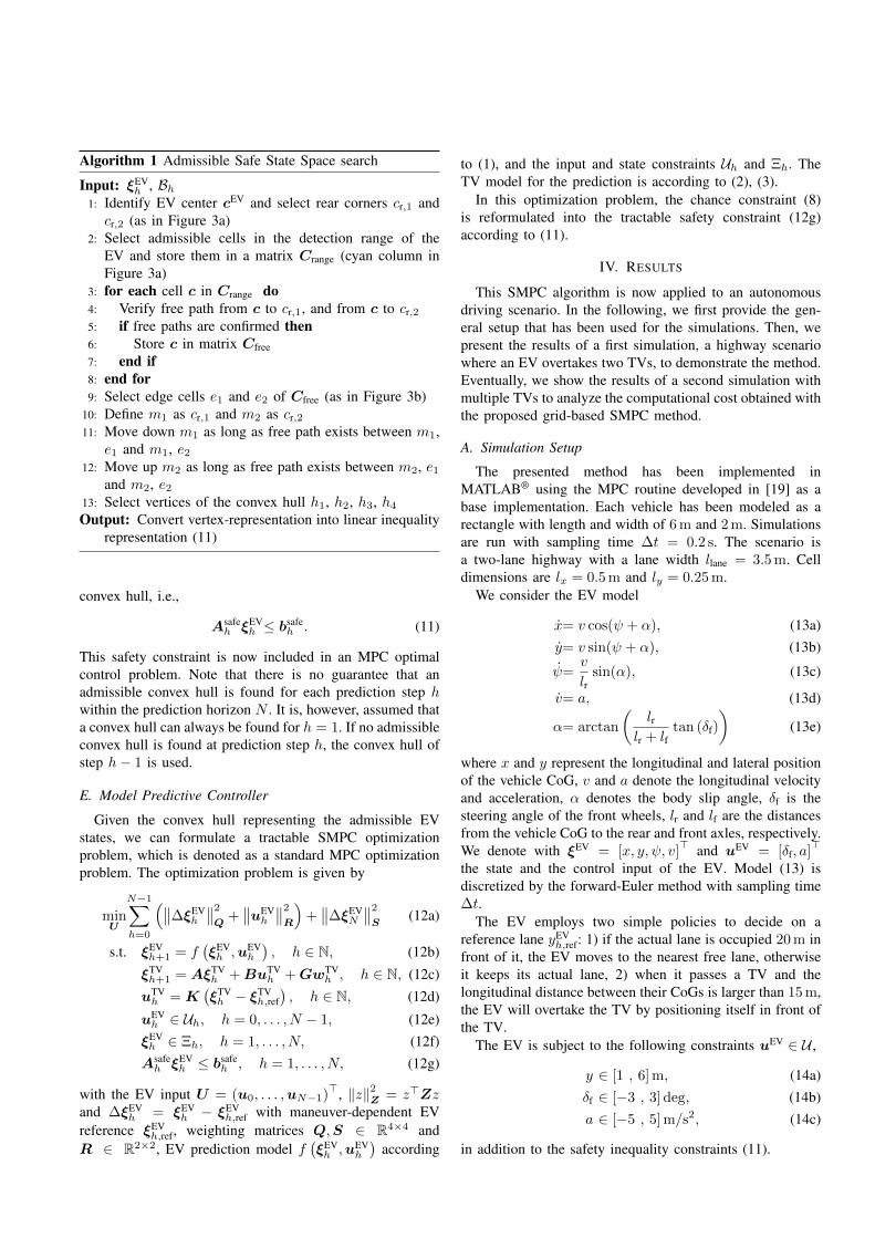
The basic steps are shown in Figure 3, where the bluecells represent the EV vehicle and the gray cells represent theinadmissible space according to (9). The scenario is a straightroad with direction of motion along the x-axis. First, validcells in the EV detection range are determined (Figure 3a).Then, using Bresenham’s algorithm, it is checked whetherthe cells on the detection range boundary allow straightconnecting lines to the EV without intersecting occupiedcells. Second, the area of valid cells around the EV is

enlarged (Figure 3b), resulting in a convex hull (Figure 3c).The detailed approach is described in Algorithm 1.

(a) The yellow cell represents the EV center cEV, brown cells showthe rear corners of the EV, cyan cells (Crange) indicate the cellsin the (approximated) EV detection range. Bresenham’s algorithmevaluates if cells are free between the rear corner cells and thedetection range cells (orange line). If a free path from a cell c ofCrange to both cr,1 and cr,2 is verified, the cell is marked with agreen color (Cfree), otherwise with red.

(b) The edges of the green column are marked as e1 and e2. Toobtain a larger convex hull, the rear corner cells are moved outsidethe vehicle bounds if connections are possible to e1 and e2 withoutintersecting inadmissible cells.

(c) The light-blue area displays the convex hull, the vertices aremarked with orange cells.

Fig. 3: Illustration of the steps in Algorithm 1.

Algorithm 1 is used for each time step h of the predictionhorizon N . It results in a linear inequality description of a

Algorithm 1 Admissible Safe State Space search

Input: ξEVh , Bh

1: Identify EV center cEV and select rear corners cr,1 andcr,2 (as in Figure 3a)

2: Select admissible cells in the detection range of theEV and store them in a matrix Crange (cyan column inFigure 3a)

3: for each cell c in Crange do4: Verify free path from c to cr,1, and from c to cr,25: if free paths are confirmed then6: Store c in matrix Cfree7: end if8: end for9: Select edge cells e1 and e2 of Cfree (as in Figure 3b)

10: Define m1 as cr,1 and m2 as cr,211: Move down m1 as long as free path exists between m1,

e1 and m1, e212: Move up m2 as long as free path exists between m2, e1

and m2, e213: Select vertices of the convex hull h1, h2, h3, h4Output: Convert vertex-representation into linear inequality

representation (11)

convex hull, i.e.,

Asafeh ξEV

h ≤ bsafeh . (11)

This safety constraint is now included in an MPC optimalcontrol problem. Note that there is no guarantee that anadmissible convex hull is found for each prediction step hwithin the prediction horizon N . It is, however, assumed thata convex hull can always be found for h = 1. If no admissibleconvex hull is found at prediction step h, the convex hull ofstep h− 1 is used.

E. Model Predictive Controller

Given the convex hull representing the admissible EVstates, we can formulate a tractable SMPC optimizationproblem, which is denoted as a standard MPC optimizationproblem. The optimization problem is given by

minU

N−1∑h=0

(∥∥∆ξEVh

∥∥2Q

+∥∥uEV

h

∥∥2R

)+∥∥∆ξEV

N

∥∥2S

(12a)

s.t. ξEVh+1 = f

(ξEVh ,uEV

h

), h ∈ N, (12b)

ξTVh+1 = AξTV

h +BuTVh +GwTV

h , h ∈ N, (12c)

uTVh = K

(ξTVh − ξTV

h,ref

), h ∈ N, (12d)

uEVh ∈ Uh, h = 0, . . . , N − 1, (12e)ξEVh ∈ Ξh, h = 1, . . . , N, (12f)Asafe

h ξEVh ≤ bsafe

h , h = 1, . . . , N, (12g)

with the EV input U = (u0, . . . ,uN−1)>, ‖z‖2Z = z>Zz

and ∆ξEVh = ξEV

h − ξEVh,ref with maneuver-dependent EV

reference ξEVh,ref, weighting matrices Q,S ∈ R4×4 and

R ∈ R2×2, EV prediction model f(ξEVh ,uEV

h

)according

to (1), and the input and state constraints Uh and Ξh. TheTV model for the prediction is according to (2), (3).

In this optimization problem, the chance constraint (8)is reformulated into the tractable safety constraint (12g)according to (11).

IV. RESULTS

This SMPC algorithm is now applied to an autonomousdriving scenario. In the following, we first provide the gen-eral setup that has been used for the simulations. Then, wepresent the results of a first simulation, a highway scenariowhere an EV overtakes two TVs, to demonstrate the method.Eventually, we show the results of a second simulation withmultiple TVs to analyze the computational cost obtained withthe proposed grid-based SMPC method.

A. Simulation Setup

The presented method has been implemented inMATLAB® using the MPC routine developed in [19] as abase implementation. Each vehicle has been modeled as arectangle with length and width of 6 m and 2 m. Simulationsare run with sampling time ∆t = 0.2 s. The scenario isa two-lane highway with a lane width llane = 3.5 m. Celldimensions are lx = 0.5 m and ly = 0.25 m.

We consider the EV model

x= v cos(ψ + α), (13a)y= v sin(ψ + α), (13b)

ψ=v

lrsin(α), (13c)

v= a, (13d)

α= arctan

(lr

lr + lftan (δf)

)(13e)

where x and y represent the longitudinal and lateral positionof the vehicle CoG, v and a denote the longitudinal velocityand acceleration, α denotes the body slip angle, δf is thesteering angle of the front wheels, lr and lf are the distancesfrom the vehicle CoG to the rear and front axles, respectively.We denote with ξEV = [x, y, ψ, v]

> and uEV = [δf, a]>

the state and the control input of the EV. Model (13) isdiscretized by the forward-Euler method with sampling time∆t.

The EV employs two simple policies to decide on areference lane yEV

h,ref: 1) if the actual lane is occupied 20 m infront of it, the EV moves to the nearest free lane, otherwiseit keeps its actual lane, 2) when it passes a TV and thelongitudinal distance between their CoGs is larger than 15 m,the EV will overtake the TV by positioning itself in front ofthe TV.

The EV is subject to the following constraints uEV ∈ U ,

y ∈ [1 , 6] m, (14a)δf ∈ [−3 , 3] deg, (14b)a ∈ [−5 , 5] m/s2, (14c)

in addition to the safety inequality constraints (11).

We consider a time-discrete point-mass TV predictionmodel for (2) with

A =

1 ∆t 0 00 1 0 00 0 1 ∆t0 0 0 1

, B =

0.5 (∆t)

20

∆t 0

0 0.5 (∆t)2

0 ∆t

. (15)

The selected TV controller matrix values are[k12, k21, k22] = [−1,−0.8,−2.2]. We assumeGaussian noise wTV

k ∼ N (0,Σw) with covariancematrix Σw = diag (1, 1, 1, 1) and disturbance matrixG = diag (0.05, 0.067, 0.013, 0.03). These choices for theTVs are similar to [11].

Here, only the two most likely TV maneuvers are con-sidered: a lane keeping (LK) and a lane changing (LC)maneuver with constant longitudinal velocity where each ofthem is weighted with a probability value for the respectivemaneuver being executed, as shown in Sec. III-B. Note thatmore maneuvers could be considered. Here, we randomlyassign a probability in the range of [0.8 , 1] to one ofthe predicted maneuvers. The second maneuver is given aprobability such that the sum equals one.

The SMPC has a prediction horizon N = 20, weightingmatrices Q = diag (0, 2, 0.5, 0.1) and R = diag (0.1, 1), anda probability threshold pth = 0.15.

Algorithm 1 is used to find a convex hull at each timestep h of the prediction horizon N . If at a generic timestep ht a convex hull is not found, we consider the onecalculated at the preceding time step ht − 1. Therefore,Algorithm 1 is based on the assumption that a convex hullcan always be found at step h = 0.

B. Overtaking Scenario

This scenario consists of a straight two-lane road with twoTVs. The center of the right lane is set to 1.75 m, the left laneto 5.25 m. The EV is positioned on the left lane with initialstate ξEV = [10, lref, 0, 26], where lref = 5.25 m. The twoTVs start with the initial states ξTV1 = [40, 27, 5.25, 0], andξTV2 = [90, 27, 1.75, 0]. TV1 is positioned on the left lane,TV2 on the right one. A probability value 0.8 is assignedto the LK maneuver and 0.2 to the LC maneuver for bothTVs. In the simulation the TVs follow the maneuver with thehigher probability. Therefore, both TVs will actually proceedalong their lane.

Figures 4, 5, and 6 show the simulation results. Figure 4illustrates the vehicle motion, Figure 5 displays the EV ve-locity and steering angle, while Figure 6 shows the distancebetween the EV and the two TVs. At the beginning theEV accelerates to reach its reference velocity of 30 m/s,as shown in the first plot of Figure 5. When the laneis occupied by TV1 20 m in front of the EV, the EVstarts a LC maneuver, moving to the right lane, as shownin Figure 4a. In Figure 6a it can be seen that once themaneuver is completed, the longitudinal distance betweenEV and TV1 is approximately 16 m. As soon as it passesTV1 and the distance between their CoGs is larger than15 m, the reference lane for the EV changes and the EV

starts to move towards the left lane to finish overtaking TV1.Figure 4b shows a screenshot of this phase. When the EVhas completed the maneuver, i.e., when it lies completelyin the left lane, the longitudinal distance with respect toTV1 is about 17 m. Once it reaches and passes TV2, the EVperforms a new LC maneuver by moving to the right laneagain. Once the EV lies on the right lane, the relative distancebetween the CoGs of the two vehicles is approximately 21 m.This last phase is represented in Figure 4c.

For the presented scenario, and with the given policies,we can see that there is no deceleration by the EV whileperforming LC maneuvers, but only changes in the steeringangle ψ. Collisions are avoided. As the simulated (not thepredicted) TV motion is deterministic in this scenario, onesimulation is sufficient for the proposed method. For thepresented grid-based SMPC method, additional simulationswith identical initialization result in the same behavior, incontrast to SMPC methods based on sampling.

Given this setup and the policy to compute the referencelane for the EV, the MATLAB® solver fmincon always findsa feasible solution. Therefore, bounds on control signal andspace constraints are respected. However, it is important tomention that these results are obtained with the choice pth =0.15, and no further research has been conducted on differentvalues. The effect of varying risk parameters is studied inother SMPC works, e.g., [7], [11].

C. Computational cost evaluation

To evaluate the computational cost of the algorithm, weuse the following more complex setup. The general setupis the one shown in Section IV-B. For each simulation, theEV is randomly positioned on one of the two lanes and arandom reference lane is assigned. The same applies to eachTV. The first TV is positioned in front of the EV with alongitudinal distance of 40 m. If more TVs are simulated,these are positioned every 50 m. For each TV, one probabilityvalue is sampled in the range [0.8 , 1] and assigned randomlyto one of the two maneuvers, LC or LK, and the secondvalue is assigned to the other maneuver such that the sumof the probabilities equals one. The actual behavior of a TVfollows the maneuver with higher probability. We simulatedthree scenarios with one, two, and three TVs, and each ofthem has been run 10 times on a standard desktop computerwith an Intel i5 processor (3.3 GHz).

Table I shows the mean µ and the standard deviation

TABLE I: Mean and standard-deviation per algorithm itera-tion for scenarios with a different number of TVs .

# of TVs µ (s) σ (s)

1 TV 0.45 0.48

2 TVs 0.44 0.43

3 TVs 0.42 0.36

σ of the algorithm computation time per iteration. Byincreasing the number of TVs in the EV detection range

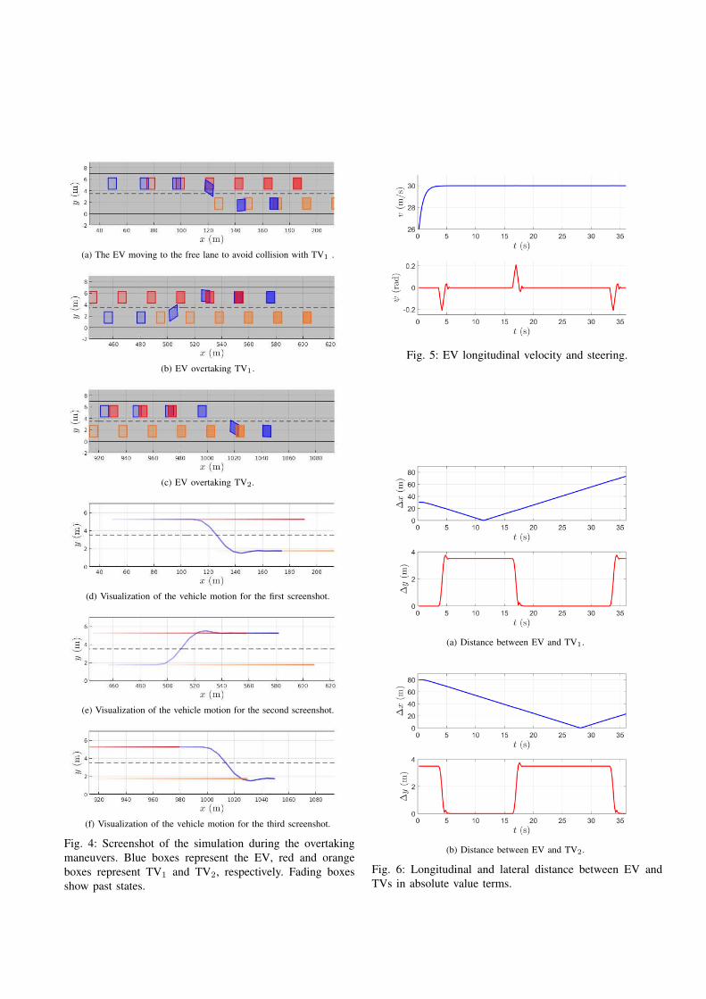
(a) The EV moving to the free lane to avoid collision with TV1 .

(b) EV overtaking TV1.

(c) EV overtaking TV2.

(d) Visualization of the vehicle motion for the first screenshot.

(e) Visualization of the vehicle motion for the second screenshot.

(f) Visualization of the vehicle motion for the third screenshot.

Fig. 4: Screenshot of the simulation during the overtakingmaneuvers. Blue boxes represent the EV, red and orangeboxes represent TV1 and TV2, respectively. Fading boxesshow past states.

Fig. 5: EV longitudinal velocity and steering.

(a) Distance between EV and TV1.

(b) Distance between EV and TV2.

Fig. 6: Longitudinal and lateral distance between EV andTVs in absolute value terms.

for the scenario, the computation cost mean µ remainsalmost constant, while the standard deviation σ shows largervariations. The computational cost of the algorithm is mainlydue to the complexity of the nonlinear EV model (13), andnot dependent on the number of TVs in the scenario. Thecomputational effort generating the PG and calculating theconvex hull is comparatively small, as this is done prior tosolving the optimization problem. This is a major advantageover for example [11], where the computation time increasessignificantly with an increasing number of TVs.

D. Discussion

In Section III-C we introduced the probability thresholdparameter pth, which allows to transform the PG into aBG, in order to obtain a deterministic approximation of thechance constraints (8). This parameter is a trade-off betweenconservatism and risk. By setting a low value for pth, ahigh number of cells will be considered occupied. At acertain step, the road can seem fully occupied, resulting ina conservative maneuver for the EV. On the other hand,a high value of pth will reduce the number of occupiedcells considered by the algorithm and, at certain step ofthe prediction horizon, the road can seem free. This canyield a more aggressive controller and potentially a collisionbetween the vehicles.

Therefore, the parameter pth has to be chosen by evaluatinga trade-off between conservatism and risk for the planningalgorithm, depending on the kind of distribution one decidesto adopt. It can also be beneficial to apply a time-varyingprobability threshold, adapting to different situations. Ingeneral, selecting a suitable threshold is challenging, similarto choosing a risk parameter in other SMPC approaches.Note that the risk parameter and the considered probabilityvalues do not perfectly represent true probabilities.

In the simulations a nonlinear EV model is used to in-crease the accuracy of the EV predictions, whereas a simpler,linear TV model is used in combination with noise, as theTV behavior is subject to uncertainty. However, applyinga linearized EV prediction model allows to solve a QPproblem, given the safety constraint (11), a quadratic costfunction, as well as linear input and state constraints. Thisis highly beneficial when a fast algorithm is needed that stillconsiders stochastic behavior of surrounding vehicles.

V. CONCLUSION

We presented a novel and simple approach to apply SMPCfor trajectory planning in uncertain environments, by usinga probabilistic grid. This allows efficiently planning egovehicle trajectories, while considering stochastic behaviorof surrounding objects. The proposed method scales wellwith an increasing number of objects considered, here shownfor three vehicles, and can handle arbitrary probability dis-tributions of future object motion. It is still of interest toobtain simulation results for more complex scenarios andtarget vehicle maneuvers, as well as combine the proposedapproach with occupancy grids.

While we applied the proposed method to autonomousvehicles, other applications are possible. It is especiallyinteresting to apply the grid-based SMPC approach to three-dimensional applications, e.g., trajectory planning for robots.

REFERENCES

[1] J. Levinson, J. Askeland, J. Becker, J. Dolson, D. Held, S. Kammel,J. Z. Kolter, D. Langer, O. Pink, V. Pratt, M. Sokolsky, G. Stanek,D. Stavens, A. Teichman, M. Werling, and S. Thrun. Towards fullyautonomous driving: Systems and algorithms. In 2011 IEEE IntelligentVehicles Symposium (IV), pages 163–168, Baden-Baden, Germany,June 2011.

[2] C. Katrakazas, M. Quddus, W. Chen, and L. Deka. Real-time motionplanning methods for autonomous on-road driving: State-of-the-art andfuture research directions. Transportation Research Part C: EmergingTechnologies, 60:416–442, 2015.

[3] B. Gutjahr, L. Groll, and M. Werling. Lateral vehicle trajectoryoptimization using constrained linear time-varying mpc. IEEE Trans-actions on Intelligent Transportation Systems, 18(6):1586–1595, June2017.

[4] A. Mesbah. Stochastic model predictive control: An overview andperspectives for future research. IEEE Control Systems, 36(6):30–44,Dec 2016.

[5] G. Schildbach, L. Fagiano, C. Frei, and M. Morari. The scenarioapproach for stochastic model predictive control with bounds onclosed-loop constraint violations. Automatica, 50(12):3009 – 3018,2014.

[6] T. Brudigam, J. Teutsch, D. Wollherr, and M. Leibold. Combinedrobust and stochastic model predictive control for models of differentgranularity, 2020. arXiv: 2003.06652.

[7] A. Carvalho, Y. Gao, S. Lefevre, and F. Borrelli. Stochastic predictivecontrol of autonomous vehicles in uncertain environments. In 12thInternational Symposium on Advanced Vehicle Control, Tokyo, Japan,2014.

[8] D. Lenz, T. Kessler, and A. Knoll. Stochastic model predictivecontroller with chance constraints for comfortable and safe drivingbehavior of autonomous vehicles. In 2015 IEEE Intelligent VehiclesSymposium (IV), pages 292–297, Seoul, South Korea, June 2015.

[9] G. Schildbach and F. Borrelli. A dynamic programming approach fornonholonomic vehicle maneuvering in tight environments. In 2016IEEE Intelligent Vehicles Symposium (IV), pages 151–156, June 2016.

[10] G. Cesari, G. Schildbach, A. Carvalho, and F. Borrelli. Scenario modelpredictive control for lane change assistance and autonomous drivingon highways. IEEE Intelligent Transportation Systems Magazine,9(3):23–35, Fall 2017.

[11] T. Brudigam, M. Olbrich, M. Leibold, and D. Wollherr. Combiningstochastic and scenario model predictive control to handle targetvehicle uncertainty in autonomous driving. In 21st IEEE InternationalConference on Intelligent Transportation Systems, Maui, USA, 2018.

[12] S. Thrun, W. Burgard, and D. Fox. Probabilistic robotics. MIT Press,Cambridge, Mass., 2005.

[13] C. Coue, C. Pradalier, C. Laugier, T. Fraichard, and P. Bessiere.Bayesian occupancy filtering for multi-target tracking: an automotiveapplication. International Journal of Robotic Research - IJRR, 25, 012006.

[14] M.K. Tay, K. Mekhnacha, M. Yguel, C. Coue, C. Pradalier, C. Laugier,T. Fraichard, and P. Bessiere. Probabilistic Reasoning and DecisionMaking in Sensory-Motor Systems, chapter The Bayesian OccupationFilter, pages 77–98. Springer Berlin Heidelberg, Berlin, Heidelberg,2008.

[15] M. Saval-Calvo, L. Valdes, J. Castillo-Secilla, S. Cuenca-Asensi,A. Martınez-Alvarez, and J. Villagra. A review of the bayesianoccupancy filter. Sensors, 17, 03 2017.

[16] S. Steyer, G. Tanzmeister, and D. Wollherr. Grid-based environmentestimation using evidential mapping and particle tracking. IEEETransactions on Intelligent Vehicles, 3(3):384–396, Sep. 2018.

[17] S. Steyer, C. Lenk, D. Kellner, G. Tanzmeister, and D. Wollherr.Grid-based object tracking with nonlinear dynamic state and shapeestimation. IEEE Transactions on Intelligent Transportation Systems,pages 1–20, 2019.

[18] J. Bresenham. Algorithm for computer control of a digital plotter.IBM Systems Journal, 4:25–30, 1965.

[19] L. Grune and J. Pannek. Nonlinear Model Predictive Control.Springer-Verlag, London, 2017.