On the Bernoulli property of planar hyperbolic billiards

Gianluigi Del MagnoCentro di Ricerca Matematica “Ennio De Giorgi”

Scuola Normale SuperiorePiazza dei Cavalieri 3

56100 Pisa, Italyemail: g.delmagno@sns.it

Roberto MarkarianInstituto de Matematica y Estadıstica “Prof. Ing. Rafael Laguardia” (IMERL)

Facultad de Ingenierıa, Universidad de la RepublicaMontevideo, Uruguay

email: roma@fing.edu.uy

May 15, 2006

Abstract

We consider billiards in bounded non-polygonal domains of R2 with piecewise smoothboundary. More precisely, we assume that the curves forming the boundary are straight linesor strictly convex inward curves (dispersing) or strictly convex outward curves of a specialtype (absolutely focusing). It follows from the work of Sinai, Bunimovich, Wojtkowski,Markarian and Donnay [S, Bu2, W2, M1, Do, Bu4] that these billiards are hyperbolic (non-vanishing Lyapunov exponents) provided that proper conditions are satisfied. In this paper,we show that if some additional mild conditions are satisfied, then not only these billiardsare hyperbolic but are also Bernoulli (and therefore ergodic). Our result generalizes previousworks [Bu4, Sz, M3, LW, CT] and applies to a very large class of planar hyperbolic billiards.This class includes, among the others, the convex billiards bounded by straight lines andabsolutely focusing curves studied by Donnay [Do].

Contents

1 Introduction 2

2 Generalities 5

3 Main results 9

4 The induced system (Ω, ν,Φ) 11

5 Geometric optics and cone fields 135.1 Geometric optics . . . . . . . . . . . . . . . . . . . . . . . . . . . . . . . . . . . . 14

1

5.2 Cone fields . . . . . . . . . . . . . . . . . . . . . . . . . . . . . . . . . . . . . . . 155.3 Cone fields for billiards . . . . . . . . . . . . . . . . . . . . . . . . . . . . . . . . . 155.4 Discontinuities of cone fields . . . . . . . . . . . . . . . . . . . . . . . . . . . . . . 19

6 Condition B2 and hyperbolicity 196.1 Condition B2 . . . . . . . . . . . . . . . . . . . . . . . . . . . . . . . . . . . . . . 196.2 Hyperbolicity . . . . . . . . . . . . . . . . . . . . . . . . . . . . . . . . . . . . . . 20

7 A local ergodic theorem 22

8 Bernoulli property of planar billiards 278.1 Verification of Conditions E1-E6 . . . . . . . . . . . . . . . . . . . . . . . . . . . 288.2 Bernoulli Property . . . . . . . . . . . . . . . . . . . . . . . . . . . . . . . . . . . 40

9 Examples 429.1 Dispersing and focusing billiards . . . . . . . . . . . . . . . . . . . . . . . . . . . 429.2 Stadia and some semidispersing billiards . . . . . . . . . . . . . . . . . . . . . . . 439.3 Polygons with pockets and bumps . . . . . . . . . . . . . . . . . . . . . . . . . . 44

Appendices 46

A Singular sets: S±1 and V ±k 46

B Singular sets: S±k 49

C Volume estimate 55

References 56

1 Introduction

Let Q be a bounded connected open subset of the Euclidean plane R2 whose boundary Γ is anunion of finitely many compact curves of class C3. The billiard in Q is the dynamical systemgenerated by the motion of a point particle that, inside Q, moves along straight lines with unitspeed, and it is reflected by Γ so that the angle of reflection equals the angle of incidence whenthere is a collision with Γ. The billiard in Q is endowed with a natural invariant measure thatis the Liouville measure on the unit tangent bundle of Q.

In this paper, we consider a large class of planar hyperbolic billiards, and prove that theyare Bernoulli with respect to the Liouville measure. A billiard is called hyperbolic if all itsLyapunov exponents are non-zero almost everywhere. It is well known from Pesin’s theory forsmooth systems [P] and its extension to systems with singularities due to Katok and Strelcyn[KS] that a hyperbolic system has positive entropy and countably many ergodic components ofpositive measure. In addition, each ergodic component is an union of finitely many disjoint setsof positive measure with the properties that they are cyclically permuted by the dynamics, andthe first return map on each of them is K-mixing, and by general results of [CH, OW], Bernoulli.These sets are called Bernoulli components of the system. We say that a system is Bernoulli if

2

it has only one Bernoulli component. We recall that a Bernoulli system is also ergodic, sinceergodicity, mixing, K-mixing and the Bernoulli property form a hierarchy of increasingly strongstatistical properties [CFS].

The proof that a hyperbolic system is Bernoulli can be achieved by demonstrating that itsergodic components are open modulo a set of zero measure. A system having this propertyis called locally ergodic. Local ergodicity can be proved by using a simple and yet powerfulargument devised by Hopf back in the 30’s to show that geodesic flows on surfaces of negativecurvature are ergodic with respect to the volume [Ho].

The billiards considered here are not smooth systems, and some serious complications arisewhen one tries to apply Hopf’s argument to them. In fact, on the one hand Hopf’s argumentrelies on the existence of uniformly “long” stable and unstable manifolds, on the other, forbilliards, these manifolds are arbitrarily “short” as the singularities prevent them from growingin size. The way of overcoming this major obstacle was found by Sinai at the end of the60’s. In his seminal paper [S], he considered a special class of hyperbolic billiards consisting oftwo-dimensional tori with strictly convex inwards scatterers, and managed to show that theyhave “enough” stable and unstable manifolds sufficiently “long” to carry over Hopf’s argument.Sinai then went on to prove that these billiards are locally ergodic and K-mixing. The Bernoulliproperty of Sinai’s billiards was proved later in [GO].

Since the publication of Sinai’s paper, his method of proving local ergodicity has beenimproved and extended to larger and larger classes of hyperbolic systems. The papers [SC, KSS,C, M2, LW] contain extensions of Sinai’s argument valid for some classes of multidimensionalbilliards and systems with singularities (non only billiards). We will refer to results of this typeas local ergodic theorems, LET’s for short. Our proof of the Bernoulli property for the billiardsconsidered in this paper relies on a modified version of the LET proved in [LW]. We will comeback on this later.

Besides Sinai’s billiards, another important class of hyperbolic billiards is represented bysemifocusing billiards. A billiard is called semifocusing if its boundary is formed by straightlines and strictly convex outwards curves, which we will call focusing. In his famous papers[Bu1, Bu2], Bunimovich gave several examples of semifocusing billiards that are hyperbolic;the most celebrated one is certainly the so called stadium, i.e., a billiard with the shape ofa stadium. The geometry of Bunimovich’s billiards is somewhat rigid, because their focusingcurves can only be arcs of circles. The mechanism generating hyperbolicity in semifocusingbilliards was further clarified by Wojtkowski using invariant cones. He also discovered manyother focusing curves besides arcs of circles that can be used to design hyperbolic billiards[W2]. Markarian further enlarged this class of curves and also elaborated a technique to provehyperbolicity based on quadratic forms [M1]. Another class of focusing curves that can be usedto construct hyperbolic billiards was introduced by Bunimovich and independently by Donnay[Do, Bu4]. These curves are called absolutely focusing, and indeed form a large class, as itturned out that Wojtkowski’s and Markarian’s curves of class C6 and any sufficiently shortpiece of a C6 focusing curve are of this type.

The billiards considered in this paper are characterized by the following properties:

• the boundary of the billiard table is formed by finitely many curves chosen among straightlines, dispersing curves and absolutely focusing curves,

• each pair of non-flat boundary components are sufficiently apart,

3

• the subset of billiard trajectories that eventually hit only straight lines has measure zero.

The main result of this paper is the proof that the billiards just described are locally ergodic,and moreover Bernoulli if additional conditions on the smallness of the set of the non-hyperbolicbilliard trajectories are verified. Previous results of this type were obtained for dispersing andcertain semidispersing billiards [S, SC], and for semifocusing billiards like Bunimovich’s billiardsand some generalizations of these [Bu2, Bu3, Sz, LW, CT, De, DM]. We stress the fact that,in all the results just mentioned, there is a limitation on the generality of the focusing curvesadmitted in the billiard boundary, which is dropped in the results presented in this paper.

As already mentioned, to obtain our results, we use a modified version of the LET provedby Liverani and Wojtkowski [LW]. The application of this theorem in its original form or anyother LET found in literature [SC, KSS, Bu3, M2, C, LW] is not allowed in our situation,since not all the hypotheses of these theorems are verified by all the billiards that we consider.More precisely, the hypotheses of the LET in [LW] not being true for all our billiards are two:the existence of a continuous invariant cone field on the tangent bundle and a nondegeneratenoncontracting semimetric defined on stable and unstable spaces. This is so because generalabsolutely focusing boundary components have invariant cone fields that are only piecewisecontinuous [Do], and the only noncontraction semimetric we found for them is degenerate (seeSubsection 8.1). For similar reasons, we cannot use the other LET’s. To solve this problem, weprove a slight generalization of the LET of [LW] (only for two dimensional systems) that appliesto billiards with general absolutely focusing curves. In this version of the LET, the originalconditions on the continuity of the cone field and the nondegeneracy of the noncontractionmetric are replaced by weaker ones. We have to warn the reader that the proof that thehypotheses of this LET are verified by our billiards requires lengthy and sometimes involvedcomputations. And this is due, to the generality of the billiards considered.

To exemplify our results, we apply them to several hyperbolic billiards: dispersing andfocusing billiards, stadia and semidispersing billiards and billiards in polygons with pocketsand bumps. We prove that all these systems are Bernoulli. Some of our conclusions, likethose concerning dispersing and Bunimovich’s billiards, are not new. The others concerninghyperbolic billiards with general absolutely focusing curves in their boundaries are new instead.One of these new results is the proof that the convex billiards bounded by straight lines andabsolutely focusing curves studied by Donnay in [Do] are Bernoulli.

The paper is organized as follows. In Section 2, we provide some background informationon planar billiards. Section 3 is devoted to the description of the billiards studied and theformulation of the the main results of the paper. In Section 4, we introduce the first returnmap induced by the billiard map on a suitable region of the billiard phase space. We do so,because the LET that we prove applies only to the induced system rather and not to theoriginal billiard map. More generalities concerning billiards, geometric optics and invariantcone fields are given in Section 5. In particular, a detailed description of Donnay’s constructionof invariant cone fields for absolutely focusing curves is provided in Subsection 5.3. In thissubsection, we also introduce the invariant cone field for billiards used throughout this paper.One of the conditions characterizing our billiards is quite technical, and its precise formulationis given in Section 6. In this section, we also prove several results, like the hyperbolicity of ourbilliards and some properties concerning their stable and unstable manifolds used in subsequentproofs. In Section 7, we prove a LET building on the LET demonstrated in [LW]. Then inSection 8, we prove that the induced system of the billiards considered verify the hypotheses

4

of the new LET, and derive our main result: billiards with absolutely focusing curves in theboundary are locally ergodic, and moreover Bernoulli if they satisfy a mild additional conditionon the topology of the non-hyperbolic billiard trajectories. In Section 9, we consider severalexamples of billiards which our result apply to. We also study a class of billiards in polygonswith pockets and bumps that do not satisfy the additional condition mentioned above. Despitethis, we prove that they are Bernoulli. Donnay’s billiard are included in this class. Finally theappendixes contain several technical results: in Appendixes A and B, we study the regularityof the singular sets of the billiard map T and its induced system, whereas in Appendix C, weprove a lemma, certainly known but which we did not find in the literature, concerning therelation between the measure of a compact subset of a smooth curve and the volume of tubularneighborhoods of this subset.

Acknowledgments. G. D. M. was partially supported by the FCT (Portugal) throughthe Program POCTI/FEDER and by the city of Lizzanello. This paper was written while thefirst author was visiting the Instituto Superior Tecnico in Lisbon and the Centro di RicercaMatematica “Ennio De Giorgi” at the Scuola Normale Superiore in Pisa. The hospitality ofboth institutions is acknowledged gratefully. G. D. M. would also like to thank M. Lenci, C.Liverani, M. Wojtkowski, V. Donnay, J. Lopes Dias and R. Hric for useful discussions. R. M.thanks CSIC (Universidad de la Republica, Uruguay) and Proyectos Clemente Estable and PDT29/219 for financial support. Both authors would like to thank N. Chernov for enlighteningdiscussions.

2 Generalities

Let Q be a bounded connected open subset of the Euclidean plane R2. Let k ≥ 2. Weassume that its boundary Γ of is an union of n compact Ck+1 curves Γ1, . . . ,Γn that will becalled components of Γ. We also assume that Γ is a finite union of disjoint Jordan curves(homeomorphic images of the unit circle) intersecting only at their endpoints. Note that, underthese hypotheses, Q is not necessarily simply connected as it may contain a finite number oftwo-dimensional scatterers. Given a C2 curve, let κ denote its curvature. A component ofΓ is called dispersing (focusing) if it is strictly convex inward (outward) and its curvature iseverywhere non-zero. We adopt the convention that κ(·) < 0 (κ(·) > 0) on a dispersing curve(focusing curve). A point q ∈ Γ is called a corner of Γ if it belongs to several components ofΓ, otherwise it is called a regular point of Γ. For any regular point q of Γ, the symbol n(q)denotes the unit normal of Γ at q pointing inside Q.

The billiard in Q is the dynamical system generated by the motion of a point particleobeying the rule: inside Q, the particle moves along straight lines at unit speed, and when theparticle hits Γ, it gets reflected so that the angle of reflection equals the angle of incidence. Thebilliard in Q can be described either by a flow (billiard flow) or a map (billiard map). In thispaper, we will focus our attention on the billiard map that is introduced below. For a definitionand detailed discussion of the properties of the billiard flow, we refer the reader to the book[CFS]. Finally a word about the terminology used throughout the paper: we will use the wordsmooth as synonym of C1.

5

Billiard phase space. Consider a smooth component Γi of Γ, and assign an orientationto it. For a given unit tangent vector (q, v) ∈ T1R2, let θ(q, v) denote the angle that theoriented tangent of Γi at q forms with (q, v). If Γi is not a closed curve, and q is an endpointof Γi, then the one-sided tangent has to be taken in this definition. We assume that theorientation of Γi is chosen so that θ(q, v) ∈ [0, π] when (q, v) points inside Q. Then the setMi := (q, v) ∈ T1R2 : θ(q, v) ∈ [0, π] collects the unit vectors attached to Γi and pointinginside Q. If s is the arclength-parameter of Γi, then the pair (s, θ) forms a a coordinate systemfor Mi. We see immediately that Mi is diffeomorphic to a cylinder or a rectangle whether ornot Γi is closed.

The billiard phase space is the set M that coincides with ∪i=1Mi after having identifiedelements of any two sets Mi and Mj with i 6= j corresponding to the same vector of T1R2.Although, in many significant cases, M is a manifolds (with boundary and corners), in general,it turns out to be a less regular object, namely, a subset of a finite union of smooth manifoldswith boundary and corners identified along subsets of their boundaries.

We close this subsection by giving few more definitions. The map π : M → Γ givenby π(q, v) = q for all (q, v) ∈ M is the canonical projection map of M onto Γ. Next letΓ−,Γ+,Γ0 be the union of the dispersing and focusing curves and the straight lines forming Γ,respectively. Then the corresponding subsets of billiard phase space are M+ := π−1(Γ+),M− :=π−1(Γ−),M0 := π−1(Γ0).

Billiard map. In the definition of the billiard map and, above all in the study of its ergodicproperties, four subsets of the billiard phase space play a key role. The first set S1 consists ofunit vectors attached at the endpoints of non-closed components of Γ, and the second set S2

consists of the unit tangent vectors of the components of Γ. Formally S1 = ∪i=1∂Γi × [0, π]where the union is taken over all non-closed components of Γ, and S2 = ∪i=1Γi × 0, π. Let∂M = S1 ∪ S2 and intM = M \ ∂M . For any z = (q, v) ∈ intM , let L(z) = q + tv : t ≥ 0that is the ray starting at q and parallel to v. Then define q1 = q1(z) to be the point inthe set L(z) ∩ Γ having the smallest distance from q such that q1 6= q and the segment withendpoints q and q1 is contained in the closure of Q. Clearly q1(z) is the point where z hitsfirst Γ. In order to characterize completely the collision at q1(z), we need to compute thevelocity of the particle after this collision. However such a velocity is well defined if andonly if q1 is a regular point. This fact leads us to introduce the other two subsets of Mmentioned at the beginning of this subsection. Let S3 = z ∈ intM : q1(z) is a corner of Γand S4 = z ∈ intM : L(z) is tangent to Γ at q1(z). In [KS, Part V, Theorem 6.1], it isproved that S3 and S4 are both unions of finitely many points and finitely many Ck+1 curves offinite length. We can now define the billiard map T . Let DT = intM \ S3. Then T : DT →Mis given by

T (q, v) = (q1, v1), (q, v) ∈ DT

wherev1 = v + 2〈v, n(q1)〉n(q1)

is the velocity of the particle after the collision at q1. This map is discontinuous at points of S4

and a Ck diffeomorphism on intM \ (S3 ∪ S4) onto its image.There is a natural probability measure on M that is T -invariant. In coordinates (s, θ), such

a measure is given by dµ = (2 length(Γ))−1 sin θdsdθ. Throughout this paper, we will always

6

have in mind this measure, unless we specify otherwise. We see immediately that µ(Si) = 0 for1 ≤ i ≤ 4 so that µ(DT ) = µ(M). We finally point out another important feature of the billiardmap T : the time-reversing property. More precisely, if R : M → M that reflects vectors of Mabout Γ given by R(s, θ) = (s, π − θ) for (s, θ) ∈ M , then T−1 = RTR on intM \ (S3 ∪ S4).Thanks to this symmetry, any property that is proved for T has a counterpart holding for T−1.

Singular sets. We call S+1 := S3 ∪ S4 the singular set of T . On this is the subset of M , T

is not defined or C1. Similarly there is a singular set S−1 for T−1 that, by the time-reversingsymmetry, coincides with RS+

1 . By previous observations on S3 and S4, it follows that S+1 and

S−1 are unions of finitely many points and Ck+1 curves of finite length. In Theorem A.1, weshow that the closures of S+

1 , S−1 are finite union of smooth compact curves intersecting at most

their endpoints. Since we are interesting in the dynamics of T , we need to understand howthese singular sets evolve under T . In other words, we have to compute the T -iterates of S+

1

and S−1 . For any n > 1, let S+n = S+

1 ∪ T−1S+1 ∪ · · · ∪ T−n+1S+

1 . This is the singular set of Tn,i.e., the subset of M where Tn is not defined or C1. Similarly S−n = S−1 ∪TS

−1 ∪· · ·∪Tn−1S−1 is

the singular set of T−n, and we have S−n = RS+n . We collect the singularities of all the positive

and negative powers of T into S+∞ = ∪n≥1S

+n and S−∞ = ∪n≥1S

−n , and denote by S∞ their

intersection. The last set consists of elements of M for which both the positive semi-trajectoryand the negative semi-trajectory hits a corner of Γ or hits tangentially a dispersing componentof Γ. Since all the sets S1, . . . , S4 has zero measure, it follows immediately that all the setsintroduced in this subsection have zero measure as well.

Metrics on M . In this subsection, we introduce two Riemannian metrics g and g′ for thebilliard phase space M . Selecting a suitable Riemannian metric for a specific class of billiards isquite a delicate matter. For a discussion on this issue, see, for example, Section 2.1 of [BCST].

The metric g is just the Euclidean metric ds2 + dθ2 in coordinates (s, θ). The metric g′ isdefined in terms of transversal Jacobi fields J and their derivatives J ′. Given a z ∈ M and avector u ∈ TzM , let (ds, dθ) be the components of u with respect to the basis ∂/∂s, ∂/∂θ.The transversal Jacobi field and its derivate associated to u are given by

J = sin θds,J ′ = −κ(s)ds− dθ.

(1)

J is a Jacobi field along the billiard trajectory of z and is called transversal, because it isorthogonal to that trajectory. For further readings on Jacobi fields and billiards, see [W3, Do,M4]. The metric g′ is then given by J2 + J ′2. This metric1 appeared before in several papers(for instance, [BCST]; see also the references therein) where J and g′ are called the p-norm ofu and the invariant metric, respectively. The relevance of g′ for the study of our billiards isdue to the fact that it has the Noncontraction property which is crucial for the proof of theLET (Theorem 7.5). This property is proved in Subsection 8.1. The norms corresponding to gand g′ will be denoted by ‖ · ‖ and ‖ · ‖′, respectively. We also introduce two distances on Min the following way: let w, z ∈M , if w, z ∈Mi, then d(w, z)(d′(w, z)) is equal to the distancegenerated by g(g′) on Mi, otherwise d(w, z) = 1(d′(w, z) = 1).

1Actually, g′ is a semi-metric, because it degenerates on S2.

7

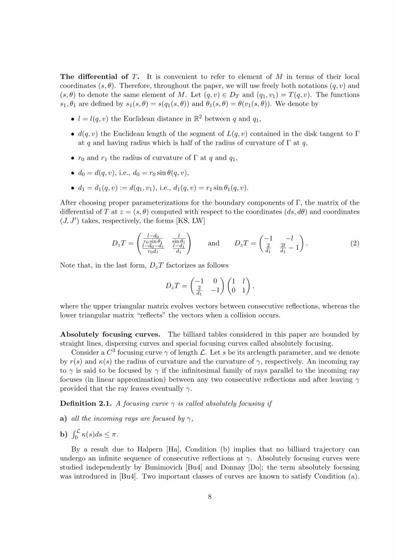
The differential of T . It is convenient to refer to element of M in terms of their localcoordinates (s, θ). Therefore, throughout the paper, we will use freely both notations (q, v) and(s, θ) to denote the same element of M . Let (q, v) ∈ DT and (q1, v1) = T (q, v). The functionss1, θ1 are defined by s1(s, θ) = s(q1(s, θ)) and θ1(s, θ) = θ(v1(s, θ)). We denote by

• l = l(q, v) the Euclidean distance in R2 between q and q1,

• d(q, v) the Euclidean length of the segment of L(q, v) contained in the disk tangent to Γat q and having radius which is half of the radius of curvature of Γ at q,

• r0 and r1 the radius of curvature of Γ at q and q1,

• d0 = d(q, v), i.e., d0 = r0 sin θ(q, v),

• d1 = d1(q, v) := d(q1, v1), i.e., d1(q, v) = r1 sin θ1(q, v).

After choosing proper parameterizations for the boundary components of Γ, the matrix of thedifferential of T at z = (s, θ) computed with respect to the coordinates (ds, dθ) and coordinates(J, J ′) takes, respectively, the forms [KS, LW]

DzT =

(l−d0

r0 sin θ1

lsin θ1

l−d0−d1r0d1

l−d1d1

)and DzT =

(−1 −l2d1

2ld1− 1

). (2)

Note that, in the last form, DzT factorizes as follows

DzT =(−1 02d1

−1

)(1 l0 1

),

where the upper triangular matrix evolves vectors between consecutive reflections, whereas thelower triangular matrix “reflects” the vectors when a collision occurs.

Absolutely focusing curves. The billiard tables considered in this paper are bounded bystraight lines, dispersing curves and special focusing curves called absolutely focusing.

Consider a C3 focusing curve γ of length L. Let s be its arclength parameter, and we denoteby r(s) and κ(s) the radius of curvature and the curvature of γ, respectively. An incoming rayto γ is said to be focused by γ if the infinitesimal family of rays parallel to the incoming rayfocuses (in linear approximation) between any two consecutive reflections and after leaving γprovided that the ray leaves eventually γ.

Definition 2.1. A focusing curve γ is called absolutely focusing if

a) all the incoming rays are focused by γ,

b)∫ L0 κ(s)ds ≤ π.

By a result due to Halpern [Ha], Condition (b) implies that no billiard trajectory canundergo an infinite sequence of consecutive reflections at γ. Absolutely focusing curves werestudied independently by Bunimovich [Bu4] and Donnay [Do]; the term absolutely focusingwas introduced in [Bu4]. Two important classes of curves are known to satisfy Condition (a).

8

The first class is formed by the so called convex scatterers introduced by Wojtkowski [W2]. Aconvex scatterer γ is a focusing curve verifying the condition

d(z) + d(z1) ≤ l(z)

for any two consecutive collisions z = (q, v) and z1 = (q1, v1) at γ. If γ is C4, then this conditionis equivalent to d2r/ds2 ≤ 0. The second class of curves satisfying Condition (a) was introducedby Markarian [M1] (see also [CM1]); these curves have the property that

d(z)(l(z) + l(z′)) ≤ l(z)l(z′)

for any two consecutive reflections z and z′ on them. Examples of Wojtkowski’s and Markarian’scurves are arcs of circles, cardioids, logarithmic spirals and the arcs of the ellipse x2/a2+y2/b2 =1, |x| ≤ a/

√2 and x2/a2 + y2/b2 = 1, |x| ≥ b4/(a2 + b2) where a, b > 0. An example of an

absolutely focusing curve which is not a Wojtkowski’s or Markarian’s curve is the half-ellipsex2/a2 + y2/b2 = 1, x ≥ 0 with a/b <

√2 [Do].

Remark 2.2. In this paper, we will only consider absolutely focusing curves of class C6. Weshould however note that our results holds as well for Wojtkowski’s and Markarian’s curveswhich are of class C4. The C6 regularity is only required for the construction of an invariantcone fields for general absolutely focusing curves (see [Do] and Section 5.3 of this paper). Itis well known that C4 Wojtkowski’s and Markarian’s curves have a continuous or a piecewisecontinuous invariant cone field with finite focusing times [W2, M1]; these two properties makeit possible to apply the results of this paper to Wojtkowski’s and Markarian’s curves.

Some important properties of C6 absolutely focusing curves are summarized here

1. Sufficiently short arcs of a focusing curve are absolutely focusing (Theorem 1 of [Do]).

2. Consider the space of focusing curves of class C6 having the same length L and satisfyingthe condition

∫ L0 κ(s)ds ≤ π. If we endow this space with the C6 topology, then the

subset of absolutely focusing curves is open (Theorem 4 of [Do]).

3 Main results

The billiards considered in this paper satisfy the following conditions besides the general onesdescribed at the beginning of Section 2.

Let N+∞ be the set consisting of elements of intM \ S+

∞ whose positive semi-trajectorieshit only Γ0 eventually. Similarly we define N−

∞ by replacing T with T−1. In fact, we couldsimply define N−

∞ := RN+∞. Both semi-trajectories of elements of N∞ := N−

∞ ∩N+∞ are infinite

and hits only Γ0 eventually so that element of N∞ are not hyperbolic. Finally let ` be theone-dimensional volume on S−1 ∪ S+

1 generated by the Euclidean metric.

B1. Each component of the boundary of the billiard table Q is either a straight line or a dispers-ing curve or an absolutely focusing curve of class C6 (C4 Wojtkowski’s and Markarian’sfocusing curves are allowed as well). Furthermore Q is not a polygon, i.e, Γ+ ∪ Γ− 6= ∅.

9

B2. The infimum of the length of all trajectories starting at any focusing component of Γ andending at any other non-flat component of Γ is uniformly bounded below by a positiveconstant depending on the focusing components of Γ.

B3. µ(N+∞) = 0 and `(N+

∞ ∩ S−∞) = 0.

The description of Condition B2 given here is somewhat vague, and we postpone a moreprecise formulation to Section 6. By now we only observe that B2 imposes some restrictionson the distance and the angle between components of Γ (see Remark 6.3). When these areWojtkowski’s and Markarian’s curves, B2 has a simple geometrical formulation in terms of therelative position of the circles of semi-curvature of distinct focusing curves [Bu2, W2], or interms of the distance of the circles of curvature of focusing curves from the other curves of Γ[M1]. As we deal with a larger class of focusing components our Condition B2 has to be moremore general, and, consequently, more involved.

Condition B3 concerns the measure of certain subsets of M supporting non-hyperbolictrajectories. The first part of Condition B3 means that the subset of trajectories which hit onlystraight lines eventually is irrelevant from the point of view of the invariant measure. This is anecessary condition to obtain hyperbolicity over the entire phase space M , and it is genericallytrue because polygonal billiards are generically ergodic [KMS]. The second part of B3 is atechnical condition, and allows to prove that the Sinai-Chernov Ansatz, one of the hypothesesof the LET (Condition E4 of Theorem 7.5), is verified. We do not know whether the secondequality of B3 is implied by the first maybe together with some simple geometric conditions onQ. Note that the time-reversing simmetry implies the symmetric equalities µ(N−

∞) = `(N−∞ ∩

S+∞) = 0.

Let NS = (N−∞∩S+

∞)∪ (N+∞∩S−∞). This set, which consists of elements of M for which one

semi-trajectory is finite, and the other hits only Γ0 eventually, also supports non-hyperbolictrajectories. The set

H := intM \ (S∞ ∪N∞ ∪NS)

contains the hyperbolic set of M . We will see that the LET applies not only to hyperbolicpoints of M but to every point of H.

A billiard (M,µ, T ) satisfying B1-B3 is hyperbolic (see Section 6). By general results onhyperbolic systems [P, KS, CH, OW], any ergodic component E of T has a finite partition(mod 0) A1, . . . , AN with N depending on E such that TAk = Ak+1, TAN = A1 and TN |Ak

is Bernoulli with respect to the probability measure µ/µ(E). Any set Ak will be called aBernoulli component of T .

The main result of this paper is the following theorem.

Theorem 3.1. For any billiard satisfying B1-B3, we have

1. the billiard map T is hyperbolic,

2. every point of H has a neighborhood belonging (mod 0) to one Bernoulli component of T .

To ensure that T is globally ergodic and Bernoulli, we need a further condition whichguarantees that the complement of H is topologically small.

B4. The set S∞ ∪N∞ ∪NS does not disconnect intMi for every 1 ≤ i ≤ n.

10

Theorem 3.2. Any billiard satisfying B1-B4 is Bernoulli.

Theorems 3.1 and 3.2 are proved in Subsection 8.2. We will see that Conditions B1-B3 implythat S∞ is countable so that the validity of B4 depends only on the topological properties ofthe sets N∞ and NS. Condition B4 can be weaken, and one can still obtain the Bernoulliproperty. In Section 9, we will consider several classes of billiards which do not satisfy B4, andeven though Theorem 3.2 cannot be applied directly to them, we will show that these billiardsare Bernoulli.

4 The induced system (Ω, ν, Φ)

In all the analysis carried out in this paper, an extremely important role is played by aninvariant cone field for the billiard dynamics. On this topic, we refer the reader to Section 5and the references therein contained. While certain billiards, like Bunimovich’s billiards andWojtkowski’s billiards, admit everywhere continuous invariant cone fields on the phase phase, itseems that general hyperbolic planar billiards can only admit a piecewise invariant continuouscone field (see [Do]). The discontinuity set of this field can be particularly complicated on thesubset M0 of the billiard phase space M ; this fact makes very difficult the verification of thehypotheses (in particular E4) of the LET (Theorem 7.5) which is the central result in the proofof the Bernoulli property of hyperbolic billiards. To overcome this problem, we will work witha new system (Ω, ν,Φ) which is the first return map induced by T on a suitable subset Ω of M .It turns out that it is much easier to deal with the discontinuity set of the invariant cone fieldof Φ (see Subsection 5.3) than with that of T . In Section 8, we will show that Φ satisfies thehypotheses of Theorem 7.5, and then that the conclusion of this theorem is valid for T as well.Throughout this section, we will use several results proved in Appendix.

Given a smooth curve γ ∈ M , we denote by int γ, ∂γ, γ, respectively, the interior, theboundary and the closure of γ in the relative topology of γ. Given two points q1, q2 ∈ R2, let(q1, q2) be the open segment joining q1, q2.

Definition 4.1. We say that a set Λ ⊂M is regular if its closure is an union of k > 0 smoothcompact curves γ1, . . . , γk such that γi ∩ γj ⊂ ∂γi ∩ ∂γj for i 6= j.

Definition 4.2. A compact and connected set B ⊂ M is called a box if B coincides with theclosure of int and ∂B is a regular set.

In the following, the symbol B will always denote a finite union of boxes of M intersectingat most at their boundaries.

Definition 4.3. Let Λ ⊂ B be a regular set, and γ1, . . . , γk be smooth compact curves as inDefinition 4.1. We say that Λ is neat in B if ∂γi ⊂ ∂B∪ (∪j 6=iγj) for any 1 ≤ i ≤ k. The wordneat alone is used in place of neat in M .

Remark 4.4. If Λ is neat in B, then it is easy to show that Λ partitions B, meaning thatthere exist k > 0 boxes B1, . . . , Bk contained in B such that intB1, . . . , intBk are the connectedcomponents of intB \ Λ.

11

Definition 4.5. Let V +1 = S+

1 ∩M0, and for k > 1, define inductively

V +k = (T−1V +

k−1 ∩M0) ∪ V +1 .

We define similarly V −n by replacing S+

1 , T−1 by S−1 , T . The sets V ±

k consist of elements ofM0 having at most k− 1 consecutive collisions with Γ0 before hitting a corner of Γ or having atangential collision at Γ−. Let Vk = V −

k ∪ V +k , and ∂M0 = ∂M ∩M0.

Lemma 4.6. Vn partitions M0 into N = N(n) > 0 boxes B1, . . . , BN such that for every1 ≤ i ≤ N only one of the following possibilities can occur:

1. T j intBi ⊂M0 for any 0 ≤ j ≤ n− 1,

2. ∃ 0 ≤ k < n− 1 such that T j intBi ⊂M0 for any 0 ≤ j ≤ k and T k+1 intBi ⊂M− ∪M+.

The same is true if T is replaced by T−1.

Proof. To prove that Vn partitions M0, it is enough to show that Vn is neat. This is a conse-quence of Corollary A.5 and the finiteness of V +

n ∩ V −n . The last fact can be proved as follows.

By Corollary A.5, the sets V +n , V

−n are finite unions of proper sets of type Cm

i (see DefinitionA.2). Consider two of such sets Cm

i , Cm′

i ′such that Cm

i ∈ V +n and Cm′

i ′∈ V −

n . Let γ1 be theclosure of a connected component of Cm

i , and γ2 be the closure of a connected component ofCm′

i ′. We are done, if we show that γ1 ∩ γ2 is finite. For i = 1, 2, let Ii 3 t 7→ γi(t) be a regular

parametrization of γi where Ii is a closed interval. We have γi(t) = (si(t), θi(t)) in coordinates(s, θ). It is easy to check that s′1θ

′1 > 0 for any t ∈ int I1, and s′2θ

′2 < 0 for any t ∈ int I2. There-

fore, in coordinates (s, θ), the curves γ1 and γ2 are strictly increasing and strictly decreasing,respectively. It follows that γ1 ∩ γ2 can contain at most one element.

We only prove the second statement of the lemma for T , because the proof for T−1 is thesame. Let

k = max0 ≤ l ≤ n− 1 : T j intBi ⊂M0 for any 0 ≤ j ≤ l.

If k = n − 1, then (1) is verified, and there is nothing to prove. Thus assume that k < n − 1.Since Vn ∩ intBi = ∅, the definition of k implies that T k intBi ∩ S+

1 = ∅. It follows that eitherT k+1 intBi ⊂M−∪M+ or T k+1 intBi ⊂M0. The latter possibility is ruled out by the definitionof k.

Definition 4.7. Let ∆n be the union of boxes Bi for which the conclusion (1) of Lemma 4.6holds, i.e.,

∆n =N⋃

i=1

Bi : T−k intBi ⊂M0 for all |k| < n.

Let Λn be the infimum of the length of the trajectories connecting ∆n and M−∪M+. Thereare two possibilities: either there is a n > 0 such that ∆n = ∅ or not, i.e., ∆n 6= ∅ for everyn > 0. In the second case, we claim that limn→+∞ Λn = +∞: this fact is only not immediatelyevident for trajectories entering one or more wedges formed by straight lines of Γ, which, onecould think, may have lots of reflections in a short amount of time. However it is easy toshow that this is not the case: such trajectories, in fact, leave a wedge after a finite number ofcollisions which only depends on the angle of wedge and not on the trajectory [CM2].

12

An example of the dichotomy pertaining ∆n is the following: if Q is a stadium-like billiardwith parallel straight lines, then we have ∆n 6= ∅ for any n > 0, but if the two straight linesare not parallel, then ∆n = ∅ for any n sufficiently large. Note that N∞ ⊂ ∩n∆n.

We choose n > 0 sufficiently large so that Λn > maxi τi + τ where the maximum is takenover all the focusing components of Γ. The constants τi and τ will be introduced in Section 6;they depend on the geometry of the billiard table Q and its invariant cone field (see Subsection5.3).

We can now define the induced system (Ω, ν,Φ). Let ∆ = ∆n.

Definition 4.8. Let Ω = M− ∪M+ ∪∆ and Φ : Ω → Ω be the first return map on Ω inducedby T , i.e., if t(z) = infk > 0 : z /∈ S+

k and T kz ∈ Ω is the first return time of z to Ω, then

Φz = T t(z)z, z ∈ Ω.

Also let ν = (µ(Ω))−1µ be a probability measure on Ω. Since Φ preserves the measure µ, it alsopreserves ν.

We stress again that the reason for introducing this new system is that for a general bil-liard satisfying B1-B3, the invariant cone field (see Section 5.3) could vary on M0 in a quitecomplicated way. For the induced systems, instead, the cone field turns out to be much nicer.

As a consequence of the definition of ∆, the space Ω is a finite union of boxes with boundarieslying on ∂M ∪ Vn. This is an important property because it allows us to apply the LET to(Ω, ν,Φ). Let ∂∆ be the boundary of ∆ and int ∆ = ∆ \ ∂∆. Furthermore let ∂Ω be the unionof ∂∆ and every ∂Mi such that Mi ⊂M−∪M+, and let intΩ = Ω\∂Ω. It is easy to check that1 ≤ t(z) ≤ 2n− 1 for every z ∈ Ω. Like T , the induced map Φ has singularities. In fact, duringthe process of inducing, in addition to the singularities produced by taking powers of T , newsingularities are created as the return time t is not constant. We denote by S+

1 the singularityset of Φ, i.e., the set of points of Ω where Φ is not defined or is not C1. The singular set for Φ−1 isdefined similarly. For k > 1, the singular set of Φk is given by S+

k = S+1 ∪Φ−1S+

1 ∪· · ·∪Φ−k+1S+1 ,

and the singular set of Φ−k is given by S−k = S−1 ∪ ΦS−1 ∪ · · · ∪ Φk−1S−1 . The union of all S+k

is denoted by S+∞, and the union of all S−k by S−∞. Note that the map Φ inherits from T the

time-reversing property, i.e., Φ−1 = RΦR, so that the singular sets of Φ−1 are just the imageunder R of the singular sets of Φ and vice-versa. We also define S∞ = S−∞ ∩ S+

∞. By previousobservations, S±k are union of finitely many smooth curves contained in S±k(3n−1). It follows thatall the sets just defined have zero ν-measure. In Proposition 8.2, we will show that S+

k and S−kare neat (as we deal now with Ω, ∂M has to be replaced by ∂Ω in the definition on neatness).

5 Geometric optics and cone fields

Invariant cone fields are used to prove hyperbolicity and statistical properties of dynamicalsystems like ergodicity, decay of correlations, etc. [W1, LW, Li]. In this section, we give thenecessary definitions, and recall some general concepts from geometrical optics. In Subsection5.3, we will introduce an invariant cone field for billiards satisfying Conditions B1 and B2.

13

5.1 Geometric optics

Variations. A variation η(α)α∈I is an one-parameter smooth family of lines in R2

η(α) = q(α) + tv(α), t ∈ R

where I = (−ε, ε), ε > 0, q, v : I → R2 are smooth, and v(α) is a unit vector for every α ∈ I.Let η(α, t) = q(α)+ tv(α), and let v⊥ be a vector orthogonal to v(0). We say that the variationη(α) focuses along η(0) if

〈 ∂η∂α

(0, t), v⊥〉 = 0 for some t ∈ R. (3)

If v′(0) 6= 0, then

t = −〈q′(0), v′(0)〉

〈v′(0), v′(0)〉is the unique solution of (3), and we call it the focusing time of η(α). When v′(0) = 0, thevariation consists, in linear approximation, of parallel lines. If 〈q′(0), v⊥〉 6= 0, then (3) doesnot have a solution, and we set t = ∞. Finally if 〈q′(0), v⊥〉 = 0, then we set t = 0. We saythat a variation is convergent, divergent or flat if its focusing time is positive, non-positive andinfinite, respectively.

Focusing times. For every vector u ∈ TzM, z ∈M , there is a family of curves inM associatedto it. Each curve ζ = (q, v) : (−ε, ε) → M of this family has the property that ζ(0) =(q(0), v(0)) = 0 and ζ ′(0) = (q′(0), v′(0)) = u. One can associate to such a curve ζ, thevariation η(α) = q(α) + tv(α), t ∈ R. The focusing time is the same for every curve ζ in thesame family so that it only depends on u, and it makes sense to call it the focusing time ofu. We say that u is convergent or divergent or flat if a variation η(α) associated to u has thecorresponding property.

For a vector u ∈ TzM , let (us, uθ) and (J, J ′) be its components with respect to the twobases described in Section 2. A straightforward computation gives (see for instance [W2])

t =sin θ

κ(s) + uθus

= − J

J ′.

the focusing time is a local coordinate of the projectivization of TzM (the space of lines inTzM) and it will be uses to describe cone fields on M . Recall that the R(s, θ) = (s, π − θ) forany (s, θ) ∈ M . The vector −u = DzRu ∈ TRzM is obtained by reflecting u about Γ at π(z).Its focusing time is given by

t =sin θ

κ(s)− uθus

.

For any u ∈ TzM, z ∈ M , let τ+(z, u) be the the focusing time of u, and let τ−(z, u) be thefocusing time of −u. Hence

τ±(z, u) =sin θ

κ(s)± uθus

. (4)

The proof of the next statements can be found in [W2, Do].

14

Reflection Law. Let z = (s, θ) ∈ DT , and Tz = (s1, θ1). For any u ∈ TzM , let τ0 = τ+(z, u),and let τ1 = τ+(Tz,DzTu). The relation between τ0 and τ1 is given by

1τ1

+1

l(z)− τ0=

2κ(s1)sin θ1

. (5)

Ordering property. Let z ∈ DT such that Tz ∈ M+, and let u,w ∈ TzM . Assume that0 < τ+(z, w) < l(z) and 0 < τ+(Tz,DzTw). Then, as a direct consequence of (5), we obtain

τ+(z, u) ≤ τ+(z, w) ⇒ 0 < τ+(Tz,DzTu) ≤ τ+(Tz,DzTw).

The implication is also true if we replace the inequalities with strict inequalities.

5.2 Cone fields

Let V be a two dimensional vector space. A cone in V is the subset C(X1, X2) = aX1 + bX2 :ab ≥ 0 where X1 and X2 are linearly independent vectors of V and a, b real numbers. If 0denotes the zero element of V , then intC(X1, X2) = aX1 + bX2 : ab > 0 ∪ 0 is the interiorof C. The cone C ′(X1, X2) := C(X1, X2) is called the complementary cone of C(X1, X2).

Definition 5.1. A measurable cone field C on the billiard phase space M is a family of conesC(z) = C(X1(z), X2(z)) ⊂ TzM defined for µ-almost z ∈ M such that the vectors X1(z)and X2(z) vary measurably with z. We say that the cone field C is invariant (strictly) ifDzTC(z) ⊂ C(Tz) (intC(Tz)) for µ-almost every z ∈M . We say that C is eventually strictlyinvariant if it is invariant, and for µ-almost every z ∈ M there exists a positive integer m(z)such that DzT

m(z)C(z) ⊂ intC(Tm(z)z). Let C ′ denote the complementary cone field of C.

For every z ∈M , define

τ+(z) = supu∈C(z)

τ+(z, u),

τ−(z) = supu∈C′(z)

τ−(z, u).

The next lemma provides a simple criterion for checking whether a cone field on M+ isinvariant. For its proof, see [Do].

Lemma 5.2. Let z ∈ M+ ∩DT such that Tz ∈ M+. Suppose that 0 ≤ τ+(z), τ−(Tz) ≤ l(z).Then

0 < τ+(z) + τ−(Tz) ≤ (<) l(z) ⇒ DzTC(z) ⊆ C(Tz) (intC(Tz)).

5.3 Cone fields for billiards

Following [S, W1, Do], we introduce a cone field C on the restricted phase space Ω for billiardssatisfying Condition B1. In Section 6, we will show that if Condition B2 and B3 are also verified,then C is eventually strictly invariant. This cone field is not everywhere continuous, and so, inthe last part of this section, we study its discontinuity set.

15

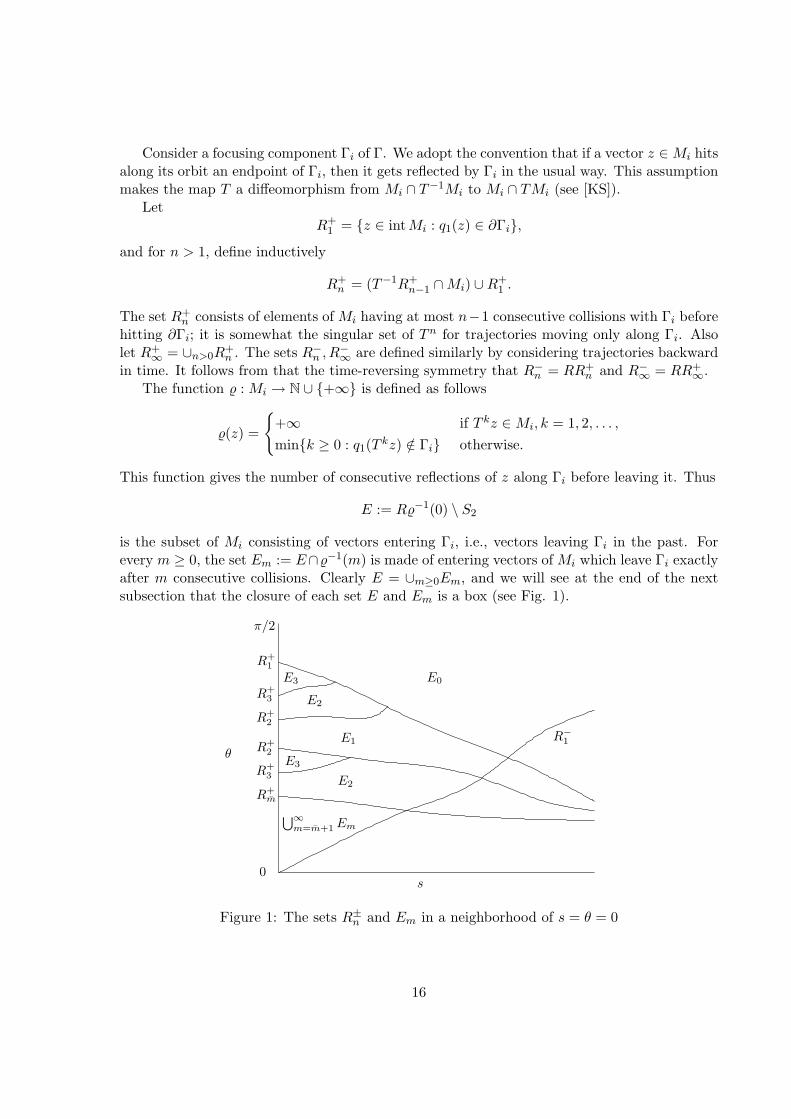
Consider a focusing component Γi of Γ. We adopt the convention that if a vector z ∈Mi hitsalong its orbit an endpoint of Γi, then it gets reflected by Γi in the usual way. This assumptionmakes the map T a diffeomorphism from Mi ∩ T−1Mi to Mi ∩ TMi (see [KS]).

LetR+

1 = z ∈ intMi : q1(z) ∈ ∂Γi,

and for n > 1, define inductively

R+n = (T−1R+

n−1 ∩Mi) ∪R+1 .

The set R+n consists of elements of Mi having at most n−1 consecutive collisions with Γi before

hitting ∂Γi; it is somewhat the singular set of Tn for trajectories moving only along Γi. Alsolet R+

∞ = ∪n>0R+n . The sets R−n , R

−∞ are defined similarly by considering trajectories backward

in time. It follows from that the time-reversing symmetry that R−n = RR+n and R−∞ = RR+

∞.The function % : Mi → N ∪ +∞ is defined as follows

%(z) =

+∞ if T kz ∈Mi, k = 1, 2, . . . ,mink ≥ 0 : q1(T kz) /∈ Γi otherwise.

This function gives the number of consecutive reflections of z along Γi before leaving it. Thus

E := R%−1(0) \ S2

is the subset of Mi consisting of vectors entering Γi, i.e., vectors leaving Γi in the past. Forevery m ≥ 0, the set Em := E∩%−1(m) is made of entering vectors of Mi which leave Γi exactlyafter m consecutive collisions. Clearly E = ∪m≥0Em, and we will see at the end of the nextsubsection that the closure of each set E and Em is a box (see Fig. 1).

R−1

s

R+1

R+3

R+2

R+2

E3

E1

E2

E0

E3

E2

R+m

R+3

⋃∞m=m+1Em

θ

π/2

0

Figure 1: The sets R±n and Em in a neighborhood of s = θ = 0

16

A cone field for absolutely focusing curves. We construct now the cone field C on M+.This construction is due to Donnay [Do] and is done for a single focusing component of Γi. Byrepeating it for every focusing component of Γ, we obtain C on the entire M+.

For every z ∈ E, let X−(z) and X+(z) be vectors of TzMi such that their s-component isnon-negative and

τ−(z,X−(z)) = τ+(T %(z)z,DzT%(z)X+(z)) = +∞.

The second condition means that the evolution of X−(z) backward in time gives raise to aparallel variation, and that the %(z) iteration of X+(z) forward in time, i.e., when it leaves Γi,is a parallel variation. Given a tangent vector u = (us, uθ), let m(u) := uθ/us be its slope.Using the fact that Γi is absolutely focusing, one can easily check that

• −κ(z) < m(X+(z)) < m(X−(z)) = κ(z) for any z ∈ E,

• X− is continuous on E, and X+ is continuous on every Em.

Suppose now that there exists a unit vector field Xl on E such that

1. m(X+(z)) < m(Xl(z)) < m(X−(z)) for any z ∈ E,

2. supz∈Eiτ−(z,Xl(z)) and supz∈Ei

τ+(Φ%(z)z,DzΦ%(z)Xl(z)) are both finite.

These conditions say that the vector Xl(z) leaves Γi after finitely many collisions, that it focusesbetween any two of such collisions and after the last one, and that the focusing times beforethe first and the last collisions are uniformly bounded on z ∈ E. If we define

CE(z) := C

(∂

∂θ(z), Xl(z)

), z ∈ E \ S2,

or, equivalently, CE(z) := u ∈ TzE : m(Xl(z)) ≤ m(u), then Donnay’s cone field on Mi \ S2

is given byC = DzT

kCE(z) : z ∈ E and 0 ≤ k ≤ %(z).

By the properties above, and using the ordering property (see the previous subsection), we seethat every vector of C has forward and backward focusing times which are uniformly bounded.

To show the existence of a vector field Xl, we first observe that for every fixed m > 0, anylinear combination aX− + bX+ such that ab > 0 verifies Properties (1) and (2) on ∪0≤m≤mEm

(not on the entire E). We introduce now Lazutkin’s coordinates (x, y) on Mi; these are givenby

x = C1

∫ s

0r−

23 (t)dt, y = C2r

13 (s) sin

θ

2(6)

where C1 and C2 are constants depending on Γi (see [La, Do] for more details). Lemma 5.9of [Do] implies that the vector ∂/∂x verifies Properties (1) and (2) on ∪m=m+1Em for m > 0sufficiently large depending on Γi. Therefore a choice for the vector field Xl is given by

Xl(z) =

aX−(z) + bX+(z) if z ∈

⋃mm=0Em,

∂∂x(z) if z ∈

⋃+∞m=m+1Em,

for any positive a, b and m > 0 sufficiently large.

17

In this way, we obtain a family of cone fields on Mi depending on the parameters a, b, m.Note that m is the lower bound for the number of consecutive reflections of vectors in E \∪m

m=0Em. We select now a specific cone field, which will be used through all this paper, bychoosing a, b, m as follows: a, b are any two positive reals, whereas m is any sufficiently largepositive integer such that the results of Section 5 of [Do] 2 apply to ∂/∂x(z) on E\∪m

m=0Em, andthe right-hand side of (10) in the proof of Lemma 8.15 is greater than e−2(b′1+b′′1 )b3/2 (which isa constant depending only on Γ+). We observe that the smallness of the Lazutkin’s coordinatey in (8.15) is controlled by m, and that the numbers b′1, b

′′1, b3 depend on Γi. This choice of m

is technical and serves to simplify the proof of Lemma 8.15.We introduce now a quantity τi which measure how far the focusing component Γi has to

be placed from other non-flat components of Γ in order to obtain hyperbolicity. This quantityplays an important role in Condition B2 (see Section 6). Here the notation is as at the end theprevious section. Let

τ±i = supz∈Mi\S2

τ±(z) and τi = maxτ+i , τ

−i . (7)

It follows from Property (2) that τi is finite.

Remark 5.3. We observe that the choice of a, b, m effects the value of τi. We do not knowhow these parameters in order to obtain the optimal, i.e., the smallest τi. For a discussion onthis point, see also Section 4 of [Do].

By repeating the construction just described for every focusing component of Γ, we obtaina cone field on M+ \ S2. If m is the maximum of m over all focusing components of Γ, thenwe can assume that all values m are equal to m. Finally denote by τ the maximum of τi whereover all the focusing components of Γ.

A cone field for dispersing curves and straight lines (∆). To complete the constructionof C on M , it remains to define it on M− ∪∆. Using coordinates (s, θ), we set

C(z) = (us, uθ) ∈ TzM : usuθ ≤ 0, z ∈M− ∪∆.

This means that the cone C(z) consists of divergent vectors of TzM which focus inside thehalf-osculating disk of Γ at π(z) for z ∈ M−, whereas C(z) consists of all divergent vectors ofTzM for z ∈ ∆. We could have equivalently defined C on intM− ∪ int∆ as follows

C(z) =

u ∈ TzM : −|d(z)| ≤ τ+(z, u) ≤ 0 if z ∈ intM−

u ∈ TzM : τ+(z, u) ≤ 0 if z ∈ int∆.

This finishes the construction of the cone field C for billiards satisfying B1.2Donnay’s results are formulated in terms of the closeness of the angle θ to 0 or π. Large m’s correspond to

θ’s close to 0 or π.

18

5.4 Discontinuities of cone fields

We investigate now the discontinuity set C and its iterates under the map Φ.Let R±

n and E be, respectively, the union of the sets R±n and E corresponding to everyfocusing component of Γ. The sets R±

∞, Em are defined similarly. We will show, in Proposition8.2, that S+

m,S−n are neat in Ω, and that their intersection consists of finitely many points.The sets R+

m,R−n have the same properties, because they are union of smooth compact curves

contained in S+m and S−n , respectively. It follows immediately that any set of the form R+

m∪R−n

partitions M+ into finitely many boxes. Results contained in Section 5 and Appendix A2 of[Do] imply that limm→+∞ dist(R±

m, S2) = 0, where dist is the distance generated by the metricds2 + dθ2.

Using the previous observations and keeping in mind the construction of C, one can easilyprove the next proposition that collects several useful facts concerning the continuity of C.

Proposition 5.4. The cone field C has the following properties:

1. C is continuous on (∪0≤k≤mTkEm) ∪M− ∪∆ for any m > 0,

2. the restriction of C|T kEmhas a continuous extension to T kEm,

3. if D0 is the set of the discontinuities of C, then D0 ⊂ R+m+1 ∪R−

∞,

4. for k > 0, let Dk = D0 ∪ Φ−kD0, and we have Dk ⊂ S+m+1+k ∪R

−∞,

5. the closure of S+m+k+1 ∪ R

−∞ is a countable union of smooth compact curves intersecting

at their endpoints such that only finitely many curves can intersect at points of intΩ.

6 Condition B2 and hyperbolicity

In this section, we give a precise formulation of Condition B2 and give a proof of the hyperbol-icity of billiards satisfying Conditions B1-B3. The cone field C considered in this section (andthe remaining sections of this paper) is the one defined in the previous section.

6.1 Condition B2

Definition 6.1. Consider two distinct non-flat components Γi,Γj of Γ. Let di,j be the infimumof the length of the trajectories starting at Γi and ending at Γj possibly after hitting Γ0 finitelymany times. Also define

τi,j =

τi + τj if Γi,Γj ⊂ Γ+,

τi if Γi ⊂ Γ+,Γj ⊂ Γ−,0 if Γi,Γj ⊂ Γ−,

where τi is defined in (7).

Definition 6.2. We say that a corner of Γ is polygonal if it does not belong to any focusing ordispersing component of Γ. Given a focusing component Γi, let pi be the distance with respectto the Euclidean metric in R2 between Γi and the set of polygonal corners of Γ.

19

Condition B2: A billiard in a domain Q satisfies Condition B2 if there exists τ > 0 suchthat

1. di,j > τi,j + τ for any Γi,Γj ⊂ Γ+ ∪ Γ−,

2. pi > τi + τ for any Γi ⊂ Γ+.

The hyperbolicity of Φ (and T ) is just a consequence of (1). The second condition isrequired for the local ergodicity of Φ. This condition, in fact, rules out billiard tables forwhich the singular sets S+

m and S−n may have smooth components which coincide, and whenthis occurs, the singular sets may separate ergodic components of Φ. Consider, for example, amushroom-like billiard where the cap of the mushroom is a semi-ellipse (which can be chosen toabsolutely focusing, see Subsection 2), and the stem is a rectangle such that one side coincideswith the segment joining the foci of the semi-ellipse and the other side is sufficiently long (saylarger than twice the major axis of the semi-ellipse). This billiard is not locally ergodic, and,in fact, it is an example of coexistence of regular and ergodic behavior. Its phase space consistsof three invariant sets of positive measure: the billiard map is regular on two of them, andis ergodic on the third. The problem here is that two polygonal corners of this billiard lie atthe foci of the semi-ellipse. This geometry - we leave the computations to the reader - violatesCondition (2) and creates components of S+

1 and S−1 which coincide. To be more specific, weobserve that (2) allows us to prove the Neatness and the Proper Alignment of the singularsets S+

1 and S−1 , Properties E2 and E3 of the hypotheses of Theorem 7.5. One may wonderwhether the first condition of B2 indeed implies the second. The first condition imposes somerestrictions on the distance between focusing curves and polygonal corners, but it is not difficultto construct examples of billiard tables for which only (1) (and B1) is satisfied.

Remark 6.3. Condition B2 imposes several constrains on the geometry of a billiard table Q.Here are listed some of these constrains to which we will refer several times in the rest of thispaper:

i) the distance between any two non-adjacent non-flat components of Γ such that one is focusingsufficiently large,

ii) the internal angles between two adjacent focusing curves is greater than π,

iii) the internal angle between a focusing curve and a dispersing curve is greater than π,

iv) the internal angle between a focusing curve and a straight line is greater than π/2.

6.2 Hyperbolicity

We prove now the billiards verifying B1-B3 are hyperbolic, and the we discuss some propertiesof the stable and unstable manifolds of T and Φ. For billiards in convex domains bounded byabsolutely focusing curves and straight lines, the hyperbolicity was first proved in [Do].

Lemma 6.4. The maps Φ and T of billiards satisfying Conditions B1-B3 are hyperbolic.

20

Proof. First we show that the hyperbolicity of T is a consequence of the hyperbolicity of Φ.Denote by λΦ(z) and λT (z) the positive Lyapunov exponents of T and Φ at the z ∈ Ω providedthey exist. By Birkhoff’s Theorem

t(z) := limn→+∞

1n

n−1∑k=0

t(T kz)

exists for ν-a.e. z ∈ Ω where t(z) is the first return time to Ω (see Section 4). The relationbetween λΦ and λT reads as follows

λΦ(z) = t(z)λT (z), ν-a.e. z ∈ Ω.

We have 0 ≤ t(z) ≤ 2n + 1 if t(z) exists (see Section 4). Thus if λΦ(z) > 0 for ν-a.e. z ∈ Ω,then λT (z) > 0 for µ-a.e. z ∈ Ω. For µ-a.e. z ∈ M \ Ω, there exists an integer 1 ≤ k ≤ 2n+ 1such that T kz ∈ Ω. The invariance of the Lyapunov exponents implies that λT (z) > 0 for µ-a.e.z ∈M .

To prove that Φ is hyperbolic, it suffices to show that the cone field C is eventually strictlyinvariant on Ω. By Theorem 1 of [W2], then Φ has non-zero Lyapunov exponents. The proofthat C is eventually strictly invariant is standard, and we only sketch it. We have to considerthree cases: (1) z,Φz ∈ M+, (2) z ∈ M+ and Φz ∈ M− ∪ ∆, and (3) z ∈ M− ∪ ∆. UsingLemma 5.2, one can easily show that DzΦC(z) ⊂ C(Φz) in all cases. This is a straightforwardconsequence of Condition B2. In fact, C(z) is pushed strictly inside C(Φz) in all cases exceptwhen π(z), π(Φz) belong to the same focusing arc or to ∆. To finish, we observe that theabsolutely focusing property implies that every vector leaves a focusing curve after a finitenumber of reflections and, by B3, µ-a.e. vector with base point on ∆ eventually hits a focusingor dispersing curve of Γ.

Local manifolds. The fact that (Ω,Φ, ν) has non-zero Lyapunov exponents ν-a.e. does notautomatically imply the existence of local stable manifolds and local unstable manifolds ν-a.e..According to general results on systems with singularities, this happens if (Ω,Φ, ν) satisfiesConditions 1.1-1.3 of [KS, Part I]. It turns out that we do not need to check whether (Ω,Φ, ν)satisfies these conditions, because we know that the billiard map T does, and we can use thisfact to show that the local stable manifolds and local unstable manifolds of T are also localstable manifolds and local unstable manifolds of Φ. This is done in the next lemma.

Lemma 6.5. The map Φ of billiards satisfying B1-B3 has local stable manifolds and localunstable manifolds ν-a.e. on Ω. These manifolds are the intersection of the stable and unstablemanifolds of T with Ω and are absolute continuous.

Proof. In [KS, Part V], it is proved that T satisfies Conditions 1.1-1.3 of [KS, Part I]. We canthen apply Pesin’s theory to T . Since T is hyperbolic, it has local stable manifolds and localunstable manifolds µ-a.e. on M which are absolutely continuous. We claim that the connectedcomponents of these manifolds contained in Ω are local stable manifolds and local unstablemanifolds of Φ. This implies automatically that the local stable and unstable manifolds of Φare absolute continuous.

We prove the claim only for local unstable manifolds. The proof for the local stable manifoldsis similar. Let z ∈ Ω, and let W u

loc(z) be the local unstable manifold of T at z. The connected

21

component of W uloc(z) ∩ Ω containing z is a local stable manifold of Φ if the set S−k ∩W u

loc(z)does not accumulate at z as k → +∞. In fact, this intersection is empty for any k > 0, becauseW u

loc(z) is a local stable manifold of T and, by Proposition 8.2, S−k ⊂ S−k(2n−1).

7 A local ergodic theorem

In this section, we prove a LET valid for two-dimensional hyperbolic systems with singularities.As explained in the introduction, the LET’s found in literature [SC, KSS, Bu3, M2, C, LW]do not apply to the generality of the billiards satisfying B1-B3 and their induced systems. Infact, many of these billiards and their induced systems do not have a continuous invariantcone field and a special type of noncontracting metrics on their tangent stable and unstablespaces, which are among the hypotheses of the mention LET’s. Thus the need for a LET withless restrictive assumptions. The LET presented here builds on the LET proved in [LW], andapplies to systems having a piecewise continuous invariant cone field and satisfying a weak formof the Noncontraction Property (explained later in this section). We point out that even thisnew LET do not apply directly to all the billiards satisfying B1-B3, and we will use it with theinduced systems of these billiards rather than with the billiard maps themselves.

We start by describing the hypotheses of this theorem and introducing the new mathematicalobjects involved in its formulation. Let (M,m, f) be a smooth system with singularities havingthe following properties.

The phase space M. The set M is an union of n > 0 boxes M1, . . . ,Mn of R2 (seeDefinition 4.2) which can only intersect along their boundaries. The union of the interior andthe union of the boundary of the boxes of M are denoted by intM and ∂M respectively. Thespace M has a natural Riemannian metric which is the restriction of the Euclidean metric ofR2 to M. We assume that M is endowed with another Riemannian metric g which can bedegenerate on ∂M and have to satisfies certain conditions described later (see E5 and E6, laterin this subsection). We denote by ‖ · ‖ and | · | the norms generated by the Euclidean metricand g, respectively. We assume that m is absolutely continuous with respect to the volume ofthe Euclidean metric, and has bounded density which is positive on intM.

Singular sets. Let A+1 and A−1 be neat subsets of M such that f : intM\A+

1 → intM\A−1is a diffeomorphism. A+

1 and A−1 are called the singular sets of f and f−1, respectively. Forany k > 0, let A±k = A±1 ∪ f∓1A±1 ∪ . . . ∪ f∓(k−1)A±1 .

Cone field. We assume that there exists an eventually strict invariant cone field C on intM.Let D0 denote the set of the discontinuity points of C, and for any k ∈ Z \ 0, let Dk =D0 ∪ f−kD0. We assume that for any k ∈ Z \ 0, there exists a set Dk ⊂ M consisting ofat most countably many smooth compact curves intersecting at most at their endpoints suchthat Dk ⊂ Dk and Dk partitions M into countably many boxes Bii∈N. We also assume thatC|int Bi has a continuous extension from intBi up to Bi. We recall that C was assumed to beeverywhere continuous in [LW].

The previous assumptions imply that the system (M,m, f) has non-zero Lyapunov expo-nents m-a.e.. We also assume that (M,m, f) satisfies the Conditions 1.1-1.3 of [KS]. This

22

implies that there exit local stable and unstable manifolds at m-a.e. point of M, and that theyare absolutely continuous.

We introduce now two quantities that measure the expansion generated by f on the vectorsin the cone field C. These are the analogues of σ, σ∗ of [LW]. Let z ∈ intM and u ∈ TzM. IfX1(z) and X2(z) are the vectors belonging to the edges of C(z), then u = u1X1(z) + u2X2(z)for suitable u1, u2 ∈ R. Following [LW, W2], we define a quadratic form Qz : TzM → R asfollows

Qz(u) := A(X1(z), X2(z))u1u2, u ∈ TzM,

where A(·, ·) is the area form of g.

Definition 7.1. Let σkk>0, σ∗kk>0 be two families of functions σk, σ∗k : intM \ A+

k →[1,+∞) given by

σk(z) = lim infy→zy/∈Dk

infu∈int C(y)

√Qfky(Dyfku)

Qy(u), z ∈ intM\A+

k ,

and

σ∗k(z) = lim infy→zy/∈Dk

infu∈int C(y)

√Qfky(Dyfku)

‖u‖, z ∈ intM\A+

k .

For k < 0, the functions σk, σ∗k : intM\ A−k → [1,+∞) are defined similarly after replacing C

by its complementary cone.

Note that σk(z), σ∗k(z) coincide with the quantities σ(Dzfk), σ∗(Dzf

k) defined in [LW] whenz ∈ intM\Dk.

Lemma 7.2. For k > 0, the functions σk, σ∗k have the following properties:

1. σk, σ∗k are lower semicontinuous on intM\A+

k ,

2. σk, σ∗k are continuous on intM\ (A+

k ∪ Dk),

3. for any smooth compact curve γ forming Dk (see the definition of Dk), the restrictionsσk|int γ is continuous on int γ \A+

k .

The same properties holds for k < 0 with A+k replaced by A−k .

Proof. It is enough to prove the lemma for σk and when k > 0. Define

σk(y) = infu∈int C(y)

√Qfky(Dyfku)

Qy(u), y ∈ intM\ (A+

k ∪ Dk).

We recall that Dk partitions M into at most countably many boxes Bii∈Z. The assumptionsmade on C guarantee that σk can be continuously extended from intBi \ A+

k to Bi \ A+k . For

every i > 0, we define the function σ(i)k : intM\A+

k → R∪+∞ to be the continuous extension

23

of σk to Bi \ S+k , and +∞ on intM\ (A+

k ∪ Bi). Each σ(i)k is lower semicontinuous. We can

express σk in terms of the quantities σ(i)k as follows

σk(z) = minσ(i)k : z ∈ Bi (8)

for every z ∈ intM\A+k . Note that the minimum here makes sense, because we assume that only

finitely many boxes Bi’s can share the same vertex. It follows that σk is lower semicontinuous.This proves the first statement of the lemma.

To prove the second statement, it is enough to observe that if z ∈ intM\ (A+k ∪ Dk), then

σk(z) = σk(z), and that σk is continuous on M\ (A+k ∪ Dk).

It remains to prove the third statement of the lemma. Let γ be one of the curves formingDk; clearly γ belongs to the boundary of two boxes Bi’s. As σ(i)

k is continuous on Bi \ A+k , it

follows that σ(j)k |int γ\A+

kis continuous for the (two) j’s for which γ ⊂ ∂Bj . For z ∈ int γ, we

haveσk|int γ\A+

k(z) = minσ(i)

k |int γ\A+k(z) : z ∈ int γ \A+

k .

We then see that σk|int γ\A+k

is continuous.

Lemma 7.3. The function σk has the following properties:

1. σk ≥ 1,

2. σk is supermultiplicative, i.e., σk1+k2(z) ≥ σk2(fk1z)σk1(z) for any positive integers k1, k2,

3. limk→±∞ σk(z) = +∞ if and only if limk→±∞ σ∗k(z) = +∞.

Proof. Statements 1 and 2 are valid for σk, σ(i)k (see [LW, W2]). Hence they are also valid for

σk in virtue of (8). The proof of Statement 4 is as the proof of Theorem 6.8 of [LW].

The rest of the hypotheses of the LET are listed below.

E1. (Regularity) The singular sets A±k are neat for any k > 0.

E2. (Discontinuities of σ∓k) For k > 0, let Σ±k be the subset of A±1 where the restriction

σ∓k|A±1 is not defined or discontinuous. We assume that Σ±k is finite.

E3. (Proper Alignment) For every z ∈ A−1 , the tangent spaces of every smooth componentof A−1 at z is contained in C(z). A similar condition holds for points of A+

1 with C(z) replacedby its complementary cone.

E4. (Sinai-Chernov Ansatz) Letm1 be the one-dimensional measure on A+1 ∪A

−1 generated

by the Euclidean metric on R2. We have

limk→±∞

σk(z) = +∞, m1-a.e. z ∈ A∓1 .

24

E5. (Noncontraction) There exists a real number a > 0 such that for every k > 0

|Dzfku| ≥ a|u|

for any z ∈ intM and any u ∈ C(z). Furthermore a similar condition holds for k < 0 andpoints of intM\A−k with C replaced by its complementary cone.

E6. (Volume estimates) Denote by L the length generated by g. Let A be a subset of A−1 .Given δ > 0, let

Aδu = z ∈ intM : ∃W u

loc(z) and a curve γ ⊂W uloc(z)

such that ∂γ ∩A 6= ∅ and L(γ) < δ.

We assume that for any A closed in the relative topology of A−1 , there exists a positive numberc = c(A) such that

lim supδ→0+

m(Aδu)

δ≤ cm1(A).

We also assume that the same condition is verified by Aδs for any A ⊂ A+

1 closed in the relativetopology of A+

1 where Aδs is defined as Aδ

u after replacing W uloc by W s

loc.

Definition 7.4. LetH =

⋃k∈Z\0

σ−1k ((3,+∞)).

The points of H will be called sufficient.

Theorem 7.5. Let (M,m, f) be a smooth system with singularities with a cone field C verifyingall the hypotheses described earlier in this section. Then every sufficient point of M has aneighborhood contained (mod 0) in one Bernoulli component of (M,m, f).

Proof. This proof is adapted from the proof of the Main Theorem of [LW]. We assume thereader to be familiar with this proof, because, while we will describe in detail the modificationsneeded by our more general setting, we will only mention the steps of the original proof whichare still valid.

The proof of the Main Theorem occupies Sections 8-13 of [LW]. The first step of this proofis Proposition 8.4 (in Section 8). To extend the validity of this proposition to our setting, wehave to modify the part of its proof where a suitable “reference” neighborhood U ⊂ intM ofa sufficient point z is constructed. The original construction of U has to be replaced by thefollowing. We can assume without loss of generality that there exists k > 0 such that z /∈ A−kand σ−k(z) > 3. Set z = f−kz and ρ = 1/σ−k(z). Since z /∈ A−k , we can find a neighborhood Uof z such that fk is a diffeomorphism from U to fkU . Let B1, . . . , Bm be the boxes generatedby Dk and containing z. If z /∈ Dk, then there is only one box as above, and z is contained in itsinterior: in this case, the original construction in [LW] gives U . We continue with the generalcase: let Ci be the continuous extension of C|(U∩int Bi)∪fk(U∩int Bi), and Qi be the correspondingquadratic form. Then define

σ(i) = infu∈int Ci(z)

√Qi(Dzfku)Qi(u)

.

25

It is easy to see that σ−k(z) = minσ(1), . . . , σ(m). For every map fk : U∩Bi → fk(U∩Bi) andthe cone field Ci, we construct a neighborhood Ui of z in the relative topology of fk(U ∩ Bi)using the original argument of [LW]: we obtain a cone field Cρ on Ui where ρ satisfies therelation ρ < ρ < 1, and a priori depends on i. Since σ(i) ≥ σ−k(z), it is easy to see that we canchoose the same ρ for every i. Let U = ∪iUi. It is easy to check that Proposition 8.4 of [LW] isalso valid in our setting with the cone field Cρ on U just constructed.

All the results contained in Sections 9 and 10 of [LW] rely on Proposition 8.4 and generalproperties of hyperbolic systems, thus they are also valid for (M,m, f).

Section 11 of [LW] contains an improved version of the Hopf’s argument based on Sinai’sapproach [S] and valid for hyperbolic systems with singularities. This argument is the last stepof the Main Theorem of [LW]. Since it is general and relies on the results of Sections 8-10 and12-13 of [LW], it carries over to (M,m, f) if we show that the results of Sections 12 and 13extend to (M,m, f).

Sections 12 and 13 form the so called Sinai’s Theorem. This theorem provides an estimateof the m-measure of the set of the points of U which have “short” stable manifolds or unstablemanifolds (see [LW]). It consists of two parts: the first part is Proposition 12.2, the onlyresult contained in Section 12, and the second part is the Tail Bound Lemma in Section 13.Proposition 12.2 tuns out to be valid for (M,m, f) because it is a consequence of the resultscontained in Sections 8-10 [LW], and these results, as we have seen, extend to our setting. Notethat in the proof of this proposition, it is used the fact that the transformation f is a symplectic,and, since our setting is two-dimensional, the volume form generating m is a symplectic form(preserved by f).

The Tail Bound Lemma of [LW] is not valid for (M,m, f) because, among its hypotheses,there are a stronger form of our Property E5 and the continuity of C. Hence we explain nowhow the proof of this lemma has to be modified in order to work in our setting. As in [LW], wewill only deal with the unstable version of this lemma, since the stable version can be provedexactly in the same way.

Property E4 and part (4) of Lemma 7.3 imply that for m1-a.e z ∈ A−1 , we have

limk→+∞

σ∗k(z) = +∞. (9)

Given two positive numbers M, t, let

Et = z ∈ A−1 : σ∗M (z) ≤ t+ 1.

It follows from (9) that for any pair h, t > 0 there exists an integer M = M(h, t) > 0 such thatm1(Et) ≤ h. Let

BM = Σ−M ∪

(A−1 ∩ ∂M

).

If BζM denotes the ζ-neighborhood of BM in A−1 with respect to the Euclidean metric, i.e.,

BζM := z ∈ A−1 : d(z,BM ) < ζ,

then E1 and E2 implies that there exists a ζ > 0 such that the m1-measure of BζM is less than

h. Another consequence of B2 is that σ∗M |A−1 is continuous on A−1 \BζM which in turns implies

that the setsEt = z ∈ A−1 \B

ζM : σ∗M (z) ≤ t+ 1

26

andSt = z ∈ A−1 \B

ζM : σ∗M (z) ≥ t+ 1

are compact. Furthermore since Et ⊂ Et, we have m1(Et ∪ BζM ) ≤ 2h. Finally the semiconti-

nuity of σ∗M (part (1) of Lemma 7.2) implies that there exists a r > 0 such that σ∗M (z) > t forany z ∈ Sr

t where Srt is the r-neighborhood of St with respect to the Euclidean metric.

The proof now continues as in Section 13 of [LW] up to the point where CASE 1 and CASE2 are discussed. In order for the analysis of CASE 1 done in [LW] to work in our setting, weneed to make the following change: use the metric g instead of the Euclidean metric in orderto evaluate the length of f−mγ (see [LW]; note that f corresponds to T in that paper). Wecan always choose U such that its closure does not intersect ∂M. Since g can only degenerateon ∂M, the Euclidean metric and g are equivalent on U . Thus using Property E5, we obtainthat the length of f−mγ with respect to g differs from the value obtained in [LW] by a positivefactor accounting for the equivalence of the two metrics on U . To conclude the analysis ofCASE 1, we have to use Property E6, as the radius of the neighborhood of Et ⊂ Et is nowcomputed with respect to g. The analysis of CASE 2 in [LW] can be repeated word by word inour setting. However the final estimate is obtained for the Lebesgue measure, whereas we needa similar estimate for m. This follows from the latter, because, by assumption, the density ofm is bounded.

This concludes the proof of the Tail Bound Lemma and so the proof of Sinai’s Theorem for(M,m, f). To finish our proof, we need a final remark. In the formulation of the theorem ofLiverani and Wojtkowski, there is no reference to Bernoulli components of f , only to ergodiccomponents of f . Nevertheless since local stable and unstable manifolds of f are also localstable and unstable manifolds of any positive power of f , we see that as the property that Ucontains a full m-measure set of points such that any pair of them is connected by a Hopf’s chainof stable and unstable manifolds implies that U is contained (mod 0) in one ergodic componentof f so it implies that U is contained (mod 0) in one ergodic component of an arbitrary positivepower of f (in fact, any power). Thus U is contained (mod 0) in one Bernoulli component off .

Remark 7.6. Using the same argument at the end of Section 7 in [LW], one can show that if asystem (M,m, f) verifies E1-E6, then m-a.e. points of M satisfies the hypothesis of Theorem7.5 which, in turn, implies that Bernoulli components of f are open (mod 0).

8 Bernoulli property of planar billiards

We go back to billiards satisfying Conditions B1-B3. In this subsection, we prove that thehypotheses of Theorem 7.5 are verified by the induced system (Ω, ν,Φ) of these billiards endowedwith the invariant cone field C introduced in Subsection 5.3. Of course, the space Ω, the singularsets S+

k of Φ and C verify the basic hypotheses of the theorem, and we are going to check onlythat Conditions E1-E6 are verified. Once this is done, in the next subsection, will use Theorem7.5 and Condition B4 to prove that the billiard map T is Bernoulli. As we are now dealing withbilliards, the notation used through this and the following subsections is as in Sections 2-5.

27

8.1 Verification of Conditions E1-E6

Before directing our attention the proof of Conditions E1-E6, we make a remark which willsimplify our task. By the time-reverse symmetry of the billiard dynamics, we see that everyresult valid for any object defined in terms of T , is also valid for the symmetric object definedin terms of T−1. Examples of such objects are the local stable and unstable manifolds W s,W u

and the singular sets S−k ,S+k . This symmetry is somewhat incorporated in Conditions E1-E6,

as each of these conditions consists of two symmetric parts. We then see that to prove E1-E6for the billiards considered in this paper, it is enough only to check one part of each condition.This is what we will do in this section.

Consider a billiard satisfying B1-B3. Let (Ω, ν,Φ) be the corresponding induced system (seeSection 4), C the invariant cone field of (Ω, ν,Φ) (see Section 5.3), and set g = g′ where g′ isthe semimetric introduced in Section 2.

Theorem 8.1. The system (Ω, ν,Φ) verifies Conditions E1-E6.

Proof. We will show that (Ω, ν,Φ) satisfies the unstable part of E1-E6. The proof is subdividedinto Propositions 8.2, 8.5, 8.7, 8.19 and 8.22.

E1. (Regularity)

Proposition 8.2. The singular sets S±k of Φ have the following properties:

1. S±k are neat in Ω, and S±k ⊂ S±k(2n−1). In particular, (Ω, ν,Φ) verifies Condition E1.

2. S−j ∩ S+k is finite for any j, k > 0,

3. S∞ is at most countable.

Proof. Part (1). We will only prove this part of the proposition for sets S+k ; in virtue of the

relation S−k = RS+k , the result extends automatically to the sets S−k as well. We say that

S+k verifies the property (P) if it has finitely many smooth components, and it is the union

of these components. It follows from Lemma B.2 that if S+k verifies (P), then the closure of

S+k is regular. Accordingly, to prove the regularity of the closure of S+

k , we will show that S+k

verifies (P). Once this has been done, it is simple to show that S+k is neat in Ω: it is enough

to note that if the closure of a smooth component of S+k does not intersect any other smooth

component of S+k , then it can be extended up to ∂Ω.

We use an induction argument. Let us start by analyzing the case k = 1. It is clear thatit suffices to prove that S+

1 ∩ ∆ and S+1 ∩ (M− ∪M+) both verify (P). We first consider the

set S+1 ∩ ∆. The initial step is to show that (int ∆ \ V +

n ) ∩ S+n = ∅ (see Section 4 for the

definition of the quantities involved here). Suppose that this is not true, i.e., there exists aninteger 0 ≤ j ≤ n− 1 such that (int∆ \ V +

n ) ∩ T−jS+1 6= ∅. As a consequence of the definition

∆, then one obtains that T j(int ∆ \ V +n ) ∩ V +

1 6= ∅ and T j(int ∆ \ V +n ) ∩ V +

1 = ∅ are verifiedsimultaneously. Thus (int ∆ \ V +

n ) ∩ S+n = ∅. We recall that Φz = T t(z)z (see Definition

4.8). Since t on ∆ (where it is defined) has only value 1 or n, the restriction of Φ to everyconnected component of int ∆ \ V +

n is smooth, and therefore S+1 ∩∆ ⊂ V +

n ∩ int∆. It followsfrom the definition of Φ that V +

n ∩ int∆ ⊂ S+1 ∩ ∆. Hence S+

1 ∩ ∆ = V +n ∩ int∆. We have

28

V +n = ∪1≤m≤n ∪i∈Im Cm

i where the union over the i ’s is restricted as explained in CorollaryA.5. Every Cm

i has finitely many connected components whose properties are described inLemma A.3. These properties are inherited by the sets Cm

i ∩ int∆, as one can easily checkafter recalling the definition of ∆, and that V +

n ∩V −n is finite. Then it is not difficult to see that

the connected components of Cmi ∩ int∆ are smooth components of S+

1 ∩∆, and that S+1 ∩∆

verifies (P).We consider now S+

1 ∩M ′ where M ′ := M− ∪M+. Let Wn = S+1 ∪ T−1V +

2n−2. To prove(1) for S+

1 ∩M ′, we use an argument similar to the one used above for S+1 ∩ ∆. We start

by showing that S+1 ∩ (M ′ \ Wn) = ∅. Let B be any connected component of intM ′ \ Wn.

Since B ∩ S+1 = ∅, it follows that T |B is smooth and either TB ⊂ M ′ or TB ⊂ M0. In the

first case, Φ|B = T |B and Φ|B is smooth so that S+1 ∩ B = ∅. In the second case, we have

TB ∩ S+1 = ∅ because B ∩Wn = ∅, and there are two possibilities: the first is that T 2B ⊂M ′

which implies that Φ|B = T 2|B and S+1 ∩ B = ∅, and the second is that T 2B ⊂ M0 which

implies T 2B ∩ S+1 = ∅ since B ∩Wn = ∅. Then we apply the same argument to T 2B ⊂ M0

and then to the higher images of B under T . We conclude that there are three possibilities forB: i) TB ⊂ M ′, ii) there is a 1 < j ≤ 2n − 1 such that T iB ⊂ M0 for every 1 ≤ i < j andT jB ⊂ M ′, and iii) T iB ⊂ M0 for every 1 ≤ i ≤ 2n− 1. Accordingly, we have Φ|B = T j |B for1 ≤ j ≤ 2n − 1 or Φ|B = T n|B. In all cases, Φ|B is smooth so that S+

1 ∩ B = ∅. This allowsus to obtain the wanted equality (M ′ \Wn) = ∅. It is easy to check that Wn ∩M ′ ⊂ S+

1 ∩M ′,and hence S+

1 ∩M ′ = Wn ∩M ′. Corollary A.5 implies that Wn = ∪1≤m≤2n−2 ∪i∈Im Cmi where

the union over the i ′s is restricted as explained in Lemma A.3. Every connected component ofCm

i ⊂ M ′ is a smooth component of S+1 ∩M ′. By recalling the properties of the sets Cm

i andtheir connected components (Lemma A.3 and A.4), we see that S+

1 ∩M ′ verifies (P).We complete now the induction argument. We assume that S+

k verifies (P), and showthat S+

k+1 verifies (P). We have S+k+1 = Φ−1S+

k ∪ S+1 . The set S+

k is the union of its smooth

components, i.e., S+k = ∪m

i=1γi. Hence Φ−1S+k = ∪m

i=1Φ−1 int γi. As S−1 verifies (P), S−1 isthe union of its smooth components, i.e., S−1 = ∪n

j=1γ′j . The map Φ−1 is not defined at

int γi ∩ S−1 ⊂ γi ∩ S−1 ⊂ ∪nj=1γi ∩ γ′j . Using Lemma B.3, we then see that int γi ∩ S−1 is

finite, and so is the number of disjoint smooth open curves ξ(i)1 , . . . , ξ(i)l(i) forming int γi \ S−1 .

This, of course, implies that Φ−1 int γi = ∪l(i)j Φ−1ξ

(i)j . Each set Φ−1ξ

(i)j is smooth by Theorem

B.4, and, in fact, it is easy to see that it is contained in a smooth component of S+k+1. Since

Φ−1S+k = ∪m

i ∪l(i)j Φ−1ξ

(i)j , it follows that Φ−1S+

k is a finite union of smooth compact curves

contained in smooth components of S+k+1. The set S+

1 is a finite union of smooth components

of S+k+1 because S+

1 verifies (P). We have just proved that S+k+1 consists of a finite union of its

smooth components, and so S+k+1 verifies (P).

To finish the proof, we observe that Part (2) follows from Part (1) and Lemma B.3, andthat Part (3) is a consequence of Parts (1) and (2).

Lemma 8.3. The singular set S∞ of T is at most countable.

Proof. Given a z ∈ S∞, there are two integers j, k ≥ 0 such that z ∈ T kS−1 ∩ T−jS+1 . If

T iz /∈ Ω for any −k ≤ i ≤ j, then z ∈ V∞, otherwise T iz ∈ S∞ for some −k ≤ i ≤ j. Hence

29

S∞ ⊂ V∞ ∪ (∪i∈ZT−iS∞), and all we need to do is to show that V∞ and ∪i∈ZT

−iS∞ are bothat most countable. The neatness (Lemma A.5) and transversality of V −

∞ , V+∞ (see the proof

of Lemma 4.6) imply that V −∞ ∩ V +

∞ is at most countable which, it turn, implies the same forV∞ since V∞ ⊂ V −

∞ ∩ V +∞ . Proposition 8.2 implies immediately that ∪i∈ZT

−iS∞ is at mostcountable.

E2. (Discontinuities of C)

Proposition 8.4. (Ω, ν,Φ) verifies Condition E2.

Proof. According to the analysis carried out in Subsection 5.4, we can set Dk = S+m+k+1 ∪R

−∞.

To estimate the cardinality of Σ−k , we argue as follows. The set of points where σk|S−1 is not

defined is given by S−1 ∩ S+k . Let B be a box in the partition of Ω generated by Dk, and γ be

the intersection of intΩ and a smooth component of S−1 . Using Statements 2 and 3 of Lemma7.2, we see that the points where σk|γ∩B\S+

kis discontinuous are contained in

(∂ (γ ∩ intB) ∩ ∂B) ∪ (γ ∩ ∂∂B) ,

where ∂∂B is the union of the vertexes of B. Thus it is not difficult to see that

Σ−k ⊂

(S−1 ∩ S+

m+k+1

)∪

(⋃i>1

S−1 ∩R−i

)∪

(n⋃

i=1

∂γi

),

where γ1, . . . , γn are the smooth components of S−1 . The first set from the right in the previousexpression contains the branching points of S−1 , and therefore those of R−

1 . The regularityof S−1 ,S

+m+k+1 and Lemma B.3 imply that S−1 ∩ S+

m+k+1 and ∪ni=1∂γi are finite. We have

S−1 ∩R−i = ∅ for any i sufficiently large (see Case (IV) in Appendix A2 of [Do]). Using this fact

and Lemma B.2, we obtain that the set ∪i>1S−1 ∩R−i is finite. This concludes the proof.

E3. (Proper Alignment)

Proposition 8.5. (Ω, ν,Φ) verifies Condition E3.

Proof. That (Ω, ν,Φ) verifies E3 is a byproduct of the proof of Lemma B.3.

E4. (Sinai-Chernov Ansatz) Let z ∈ intΩ and u ∈ TzΩ. If X1(z) and X2(z) are non-zerovectors belonging to the edges of C(z), then we can write u = u1X1(z) + u2X2(z) for properu1, u2 ∈ R. We denote by |X1(z), X2(z)| the Euclidean area of the parallelogram with sidesX1(z), X2(z). We associate to C(z) the quadratic form

Qz(u) = sin θ|X1(z), X2(z)|u1u2, u ∈ TzΩ.

See Section 3, for the definition of S+∞ and N+

∞.

Lemma 8.6. limk→+∞ σk(z) = +∞, ∀z ∈ intΩ \ (S+∞ ∪N+

∞).

30

Proof. It is enough to prove the following property: there exists a positive number σ suchthat for any z ∈ intΩ \ (S+

∞ ∪ N+∞), one can find an increasing sequence mii∈N for which

σmi+1−mi(Φmiz) ≥ σ for every i ≥ 1. In fact, let us assume that this property is verified, and

let z ∈ intΩ \ (S+∞ ∪N+

∞) and mii∈N be the sequence associated to z. If i(n) := maxi > 0 :mi ≤ n, then, for large n, we would obtain (using the supermultiplicativity property of σ)

σn(z) ≥i(n)−1∏

i=1

σmi+1−mi(Φmiz) ≥ σ

which implies limn→+∞ σn(z) = +∞ because limn→+∞ i(n) = +∞ as a consequence of the factthat mi is increasing.

We explain now how to construct the sequence mi for a given z ∈ intΩ \ (S+∞ ∪N+

∞). Weclaim that the positive semi-trajectory of z hits non-flat components of Γ infinitely many times,and its ω-limit set cannot be equal to a corner of Γ. Suppose, in fact, that z does not have thisproperty. Since z /∈ N+

∞, the positive semi-trajectory of z hits non-flat components of Γ infinitelymany times, and so, in order to violate the property we want to prove, the ω-limit set of z mustbe a corner of Γ. This corner cannot belong to a focusing component of Γ for two reasons:the first is that focusing components of Γ are absolutely focusing, and so every trajectory canonly have a finite number of consecutive collisions with a focusing component of Γ; the secondreason is that to satisfy B2, the internal angle of the corner must be greater than either π orπ/2 according to the fact that the other component of Γ forming the corner is either a non-flatcomponent or a flat component. It is easy to see that these two facts make it impossible for thepositive semi-trajectory of z to accumulate at a corner contained in a focusing component of Γ.Thus the corner must be formed by two dispersing components or by a dispersing componentand a straight line. In both cases, however, any trajectory entering such a corner leaves it after afinite number of reflections (for example, see Appendix A1.3 of [BSC]). But then the ω-limit setof z cannot be a single corner which contradicts the assumption made on z. Let Ucusp be a smallneighborhood of the corners of Γ formed by adjacent dispersing components. For the chosen z,the sequence mi is defined recursively as follows: we set m1 = 1, and given mi for i > 1, wechoose mi+1 > mi in such a way that Φmi+1z ∈M− ∪RE and π(Φmi+1z) /∈ Ucusp. This can bedone because of the property verified by points in Ω \ (S+

∞ ∪N+∞) proved before. Next we show

that there exists a positive σ independent of z ∈ Ω \ (S+∞ ∪N+

∞) such that σmi+1−mi(Φmiz) ≥ σ

for every i ≥ 1. It is easy to show that for any i > 1, we can find an integer ki > 0 such thatT−kiΦmiz ∈ E and T−jΦmiz ∈ M0 for 1 < j < ki. Using the supermultiplicativity propertyof σ, then it is enough to show that there is σ > 0 independent of z ∈ Ω \ (S+

∞ ∪ N+∞) such

that σki(T−kiΦmiz) ≥ σ for any i > 1. This can be proved as follows. For any i > 1, let

zi = T−kiΦmiz and wi = Φmiz. Of course σki(T−kiΦmiz) = σmi(zi). we denote by li be the

length of the trajectory connecting zi, wi. To compute σki(zi), we use the Cross Ratio Formula

(see Section 1 of [W2]). This is justified by the fact that although our definition of σk(z) differsfrom that one of σ(DzT

k) in [W2], it turns out that σk(z) coincides with a certain object σ(j)k (z)

(see (8) in the proof of Lemma 7.2) for which the Cross Ratio Formula is valid. Hence thisformula is also valid for σk(z), and the cones at the points z and T kz that we have to considerfor its computation are those corresponding to σ(j)

k (z). A simple computation gives

σki(zi) =

√1 + ωi +

√ωi

31

where

ωi =

li(li−τ+(zi)−τ−(wi))τ+(zi)τ−(wi)

if zi, wi ∈M+

li(li+|d(zi)|+|d(wi)|)|d(zi)|+|d(wi)|) if zi, wi ∈M−

(li−τ+(zi))(l+|d(wi)|)τ+(zi)|d(wi)| if zi ∈M+, wi ∈M−

(li+|d(wi))(li−τ−(wi))|d(zi)|τ−(wi)

if zi ∈M−, wi ∈M+,

τ±(z) are the forward and backward focusing times of C at z (see Section 5), and d(z) is the(Euclidean) length of the segment of the trajectory of z contained in the disk tangent to Γ at qand having radius which is half of the radius of curvature of Γ at q (see Section 2). By B2 andthe definition of zi, wi, we have

li ≥ li − τ+(zi), li − τ−(wi), li − τ+(zi)− τ−(wi) ≥ τ , ∀i > 1.

If we set r := maxs∈Γ− |r(s)|, ω := τ /(max τ, r)2 and σ :=√

1 + ω +√

1 + ω, then we obtainthe wanted conclusion

σmi(zi) ≥ σ, ∀i > 1.

Proposition 8.7. (Ω,Φ, ν) verifies Condition E4.

Proof. It follows from Lemma 8.6 that it is enough to show that `(S−1 ∩ (S+∞∪N+

∞)) = 0. SinceS−1 ⊂ S−2n−1 (see Proposition 8.2) and S−∞∩Ω = S+

∞, we obtain S−1 ∩ (S+∞∪N+

∞) ⊂ (S−1 ∩S+∞)∪

(S−2n−1 ∩ N+∞). The set S−1 ∩ S+

∞ is countable by Proposition 8.2, and `(S−2n−1 ∩ N+∞) = 0 by

B3. Hence `(S−1 ∩ (S+∞ ∪N+

∞)) ≤ `(S−1 ∩ S+∞) + `(S−2n−1 ∩N+

∞) = 0.

E5. (Noncontraction) We recall ‖ ·‖′ denotes the norm generated by the semimetric g′ (seeSection 2).

Definition 8.8. Let k > 0, and z ∈ intΩ \ S+k . We say that the orbit α := z, Tz, . . . , T kz

verifies the noncontraction property if there is a constant a > 0 such that ‖DzΦku‖′ ≥ a‖u‖′for any u ∈ C(z).

The following families of orbits called blocks play an important role in the proof of E5. Weassume that z ∈ intΩ \ S+

k .

1. F1 consists of orbits z,Φz such that z ∈Mi ⊂M+ and Φz ∈Mj ∩ Ω for some i 6= j,

2. F2 consists of orbits z,Φz, . . . ,Φkz ⊂ ∆ ∪M− for some k > 0,

3. F3 consists of orbits z,Φz such that z ∈ ∆ ∪M− and Φz ∈M+,

4. F4 consists of orbits z,Φz, . . . ,Φkz ⊂Mi ⊂M+ for some k > 0 and i,

5. F5 consists of orbits z,Φz, . . . ,Φkz such that z,Φkz ∈ RE for some k > 0.

32

Remark 8.9. We observe that for the billiards considered in this paper, the noncontraction isnot always verified along every block of type 1-5 if we replace the semimetric g′ by the morenatural metric g. This is the reason why we considered g′ instead of g. It follows from theresults of this subsection and Remark 8.21 that the noncontraction is always (for any billiardconsidered here) satisfied with respect to g along blocks of type 1,4,5. It is not satisfied, instead,along all blocks of type 2 and 3. In fact, it is not difficult to construct billiard tables satisfyingB1-B3 such that there is a one-parameter family of vectors z(c) contained in F2(F3) forc ∈ (0, ε), ε > 0 such that

limε→0

θ(z(ε)) = 0 and limε→0

θ(Φz(ε)) = θ

where 0 < θ < π. It is now easy to see that if u = (1, 0) ∈ C(z(ε)), then

limε→0

‖Dz(ε)Φu‖‖u‖

= 0.

Clearly this implies that the noncontraction property is not verified with respect to g alongz,Φz.

Given a block α, we say that α is of type i(α) if α ∈ Fi(α). Every finite orbit can berepresented as a finite sequence of blocks α1, . . . , αn of type 1-4 satisfying the following rule

i(αk+1) =

i(αk) + 1 mod 4 if i(αk) ∈ 2, 3, 4,2, 4 if i(αk) = 1,

for every k = 1, . . . , n − 1. In other words, given any block representation of an orbit, we canalways reduce it to a block representation described above by grouping together adjacent blocksof the same type. We when talk about the block representation of an orbit, we will always havein mind this representation. Note that by definition a block of type 4 is allowed to contain justone element (this is important to derive the representation above), and that for an orbit of type5, its block representation α1, . . . , αn has the property that i(α1) = 1 and i(α4) = 4.

We prove now that any finite orbit can be decomposed in at most eight blocks.

Lemma 8.10. Let k > 0, and z ∈ intΩ \ S+k . There exist an integer 1 ≤ m ≤ 8 and

a finite sequence of integers 0 = k0 < k1 < · · · < km = k such that z,Φz, . . . ,Φkz =⋃mi=1Φki−1z, . . . ,Φkiz where Φki−1z, . . . ,Φkiz ∈ Fj for some 1 ≤ j ≤ 5.

Proof. Consider a finite orbit α with block representation α1, . . . , αn. After having removedthe largest block α of type 5 from α, we are left with at most two orbits, one coming before andanother coming after α. It is immediate to see that if the first of these orbits exist, then it cancontain at most three blocks; when it contains exactly three blocks, these must be a block oftype 2, one of type 3 and one of type 4. Similarly if the second orbit exists, then it can containat most four blocks; when it contains exactly four blocks, these must be a block of type 1, oneof type 2, one of type 3 and one of type 4. The orbit α admits therefore a decomposition witha maximum of 8 blocks.

To prove that (Ω, ν,Φ) has Property E5, we show, in the following series of lemmas, thatevery block of type 1-5 verifies the noncontraction property. We recall that the values τ, τ aredefined in Section 6.

33

Lemma 8.11. If z ∈M+ \ S2, then ‖u‖′/√

1 + τ2 ≤ |J ′| ≤ ‖u‖′ for any u = (J, J ′) ∈ C(z).

Proof. The lemma follows trivially from the fact that |J/J ′| ≤ τ+(z) ≤ τ for any u = (J, J ′) ∈C(z) and z ∈M+ \ S2 .

Lemma 8.12. Any block of type 1 verifies the noncontraction with constant a1 = min1/(1 +τ2)1/2, τ /τ.

Proof. Let u = (J0, J′0) ∈ C(z), and DzΦu = (J1, J

′1). We assume first that Φz ∈M− ∪∆. By

(2), we have (J1

J ′1

)=(

−1 0− 2|d(Φz)| −1

)(1 l(z)0 1

)(J0

J ′0

)where l(z) is the length of the trajectory connecting z and Φz, and the factor |d(Φz)| has to bereplaced by ∞ if Φz ∈ ∆. It follows from the construction of C on M+ that τ(z, u)J0 + J ′0 = 0.A straightforward computation then gives(

J1

J ′1

)= −

(l(z)− τ+(z, u)2 l(z)−τ+(z,u)

|d(Φz)| + 1

)J ′0.

Condition B2 implies that l(z)− τ+(z, u) ≥ τ > 0 so that |J ′1| ≥ |J ′0|. Finally

‖DzΦu‖′ ≥ |J ′1| ≥ |J ′0| ≥‖u‖′√1 + τ2

where the last inequality follows from Lemma 8.11.We assume now that Φz ∈M+. In this case, we have∣∣∣∣J ′1J ′0

∣∣∣∣ = ∣∣∣∣J ′1J1

∣∣∣∣ ∣∣∣∣J1

J ′0

∣∣∣∣ = τ−(Φz,DzΦu)τ+(Φz,DzΦu)

≥ τ

τ,

because τ−(Φz,DzΦu) = l(z)− τ+(z, u) ≥ l(z)− τ+(z) ≥ τ by B2, and τ+(Φz,DzΦu) ≤ τ byconstruction of C on M+. Using Lemma 8.11 like before, we conclude that

‖DzΦu‖′ ≥τ

τ‖u‖′.

Lemma 8.13. Any block of type 2 verifies the noncontraction with constant a2 = 1.

Proof. Let u = (J0, J′0) ∈ C(z), and DzΦu = (J1, J

′1). We prove the case when k = 1, and then

explain why it implies the general case. By (2), we have(J1

J ′1

)= −

(1 l(z)2

|d(Φz)|2l(z)|d(Φz)| + 1

)(J0

J ′0

).

where l(z) is the length of the trajectory connecting z and Φz, and the factor |d(Φz)| has to bereplaced by ∞ if Φz ∈ ∆. Since J0J

′0 ≥ 0 and l(z) > 0, it follows that |J0| ≤ |J1| and |J ′0| ≤ |J ′1|,

and therefore ‖DzΦu‖′ ≥ ‖u‖′. The invariance of C implies JiJ′i ≥ 0 for any 0 ≤ i ≤ k. Hence

the result obtained for k = 1 is valid for every segment of orbit Φiz,Φi+1z. This proves thelemma in the general case.

34

Lemma 8.14. Any block of type 3 verifies the noncontraction with constant a3 = min1, τ /τ.

Proof. Arguing exactly like in the second part of the proof of Lemma 8.12, we obtain |J ′1/J ′0| ≥τ /τ . Since J0J

′0 ≥ 0, it follows that |J1| ≥ |J0|. Hence ‖DzΦu‖′ ≥ ‖u‖′τ /τ .

Lemma 8.15. Any block of type 4 verifies the noncontraction with a certain constant a4 > 0.

Proof. To prove the lemma, it is enough to verify the noncontraction property with respect tothe seminorm |J ′|. This is justified by Lemma 8.11, and by the fact that blocks of type 4 arecontained in M+.

Let α := z,Φz, . . . ,Φkz be a block of type 4. We assume that k > 0, otherwise thereis nothing to prove. Note that Φiz = T iz for i = 1, . . . , k, and so, through this proof, we areallowed to use T instead of Φ. Let 0 6= u = (J0, J

′0) ∈ C(z), and denote (Ji, J

′i) = DzT

iu for0 ≤ i ≤ k. We have∣∣∣∣J ′kJ ′0

∣∣∣∣ = k∏i=1

∣∣∣∣J ′iJi

∣∣∣∣ ∣∣∣∣ Ji

J ′i−1

∣∣∣∣ = k∏i=1

τ−(DzTiu, T iz)

τ+(DzT iu, T iz)≥

k∏i=1

τ−(T iz)τ+(T iz)

.

Let us define

Ξ(α) =k∏

i=1

τ−(T iz)τ+(T iz)

.

The lemma is proved if we show that Ξ(α) is uniformly bounded away from zero over all blocks oftype 4. We will do this in two steps: first for blocks of type 4 contained in A := ∪m

m=0∪mi=0T

iEm,and then for blocks of type 4 contained in B := ∪∞m=m+1 ∪m

i=0 TiEm. Note that these sets are

invariant and disjoint.Let α be a block of type 4 contained in A. We recall that 0 < τ±(z) ≤ τ for any z ∈M+ \S2

by construction of C. Since A is bounded away from S2, there exists a constant C = C(m) > 0such that d(z) ≥ C for any z ∈ A. Using (5), we obtain 0 < 1/τ+(z) + 1/τ−(z) ≤ 2/C whichimplies τ±(z) ≥ C/2 for any z ∈ A. In conclusion, we have

Ξ(α) ≥(C

2τ

)m

for every block α of type 4 contained in A.Consider now a block α of type 4 contained in B. Let (x, y) be the Lazutkin’s coordinates

of z. For i = 1, . . . , k, denote by Xi be the lower edge of C(T iz) which, by construction, isequal to ∂zT

m∂/∂x(z) for some z ∈ E and m > 0. We have

τ±(T iz) =sin θ(T iz)

κ(T iz)±m(Xi)

where m(Xi) is the slope of Xi in coordinates (s′, θ′) (see Section 5.3). It follows from theresults of Section 5 of [Do] that there are constants b1, b2, b3 depending only on Γ+ such that

|m(Xi)| ≤ b1y + b2y3, i = 1, . . . , k,

andk ≤ b3

y.

35

Hence

Ξ(α) ≥(

1− b′1y − b′2y3

1 + b′′1y + b′′2y3

) b3y

(10)

where if κmax = maxΓ+ κ and κmin = minΓ+ κ, then b′i = bi/κmax and b′′i = bi/κmin for i = 1, 2.The choice of m in Section 5.3 was made to conclude that the right hand-side of this inequalityis greater than e−2(b′1+b′′1 )b3/2 which is a constant depending only on Γ+. Thus

Ξ(α) ≥ e−2(b′1+b′′1 )b3

2

for any block α of type 4 contained in B.

Definition 8.16. A block α of type 5 is called minimal if it does not contain any smaller blockof type 5. The block representation of a minimal block of type 5 is given by α1, α2, α3, α4 orα1, α4 where, in both case, it must be i(αk) = k.

It is clear that every block of type 5 decomposes into finitely many minimal blocks of type5.

Lemma 8.17. For any block z, . . . ,Φkz of type 5 containing m > 0 minimal blocks, theoperator DzΦk can be decomposed as follows

DzΦk = F−12 L2m L2m−1 . . . L1 F1.

In coordinates (J, J ′), the operators F1(F2), L2i−1, L2i have, respectively, the matrix form

(1 β0 1

), −

(1 + δ

(i)1 τ + δ

(i)3

δ(i)2 1 + δ

(i)4

),

ε(i)1 0ε(i)2

1

ε(i)1

where δ(i)1 , . . . , δ

(i)4 ≥ 0 and ε(i)1 , ε

(i)2 > 0.

Proof. It is enough to prove the lemma for a minimal block α = z, . . . ,Φkz of type 5. Let0 < k ≤ k be the integer such that Φkz ∈ α which is the first element in the sequence ofcollisions with the second focusing component of Γ visited by z. Set z0 = z, z1 = Φkz, z2 = Φkz.Using coordinates (q, v), we write zi = (qi, vi), and define pi = qi + τ+(zi)vi for i = 0, 1, 2. Nextset z0 = (p0, v0) and z1 = (p1, w1) where w1 is obtained by reflecting v1 about Γ. Finally lett0, t3 be the length of the pieces of orbit α joining q0, p0 and q2, p2, respectively, and ti be thelength of the piece joining pi−1, pi for i = 1, 2. If φtt∈R denotes the billiard flow in Q, thenwe can write DzΦk as follows

DzΦk = (Dz2φt3)−1 Dz1φt2 Dz0φt1 Dz0φt0 .

Let F1 = Dz0φt0 , F2 = Dz2φt3 , L1 = Dz0φt1 , F1 = Dz1φt2 . It is easy to check that, in coordinates(J, J ′), we have

F1 =(

1 t00 1

), F2 =

(1 t30 1

).

36

To compute the matrix form of L1, L2, we argue as follows. In coordinates (J, J ′), the vector(1, 0) represents a parallel variation, whereas (0, 1) represents a variation of lines emerging fromthe same point. Since along the orbit between p0, p1, there are only reflections at Γ− ∪ Γ0, it isnot difficult to see

L1

(10

)= −

(1 + δ1δ2

), L1

(01

)= −

(t1 + δ31 + δ4

)where δ1, . . . , δ4 ≥ 0, and the sign of the two vectors coincides. Condition B2 implies thatt1 ≥ τ so that

L1 = −(

1 + δ1 τ + δ3δ2 1 + δ4

).

Note that every variation focusing at p1 must also focus at p2. So it is easy to see that

L2

(10

)=(ε1ε2

), L2

(01

)=(

0ε3

)where ε1, ε2, ε3 > 0, and the sign of the two vectors coincides. The billiard flow in coordinates(J, J ′) preserves the standard area form. Hence detL2 = ±1, and so

L2 =(ε1 0ε2 ε−1

1

).

Lemma 8.18. Any block of type 5 verifies the noncontraction with constant a5 =√

ττ(1+τ2)

.

Proof. Consider a block of type 5 z,Φz, . . . ,Φkz containing m > 0 minimal blocks of type5. Let F1, F2, L2i, L2i−1 for i = 1, . . . ,m be the matrices associated this block as in Lemma8.17. Given u = (J0, J

′0) ∈ C(z), let (J2, J

′2) = DzΦku. Also define (J0, J

′0) = F1u, (J1, J

′1) =

L1(J0, J′0) and (J2, J

′2) = F2(J2, J

′2). We will use the symbol |u|j to denote the absolute value

of the jth component of u.By Lemma 8.11, it is enough to prove that there is a positive constant a5 such that |J ′2| ≥

a5|J ′0| for any (J0, J′0) ∈ C(z). It follows from Lemma 8.17 that there exist two 2× 2 matrices

R, R with non-negative entries such that

L2m L2m−1 . . . L3 L2 = ±(L2m L2m−2 . . . L4 L2 +R), (11)

andL2m L2m−2 . . . L4 L2 = L2m L2m−2 . . . L4 L2 + R, (12)

where

L2i =

(εi1 00 1

εi1

). (13)

If L = L2m L2m−2 . . . L4 L2 and ε =∏m

i=1 εi1, then

L =(ε 00 ε−1

). (14)

37

Let (J0, J′0) ∈ C(z), and v = (J1, J

′1). Condition B2 implies that J1/J

′1 ≥ τ so that, by using

(12) and (13), we obtain

|L2m L2m−1 . . . L3 L2v|j ≥ |Lv|j .

This gives|J2| ≥ ε|J1| ≥ ετ |J ′1|, (15)

and|J ′2| ≥ ε−1|J ′1|. (16)

Another consequence of B2 is that J2/J′2 ≤ τ . Using (15), we obtain

|J ′2| ≥ετ

τ|J ′1|. (17)

The average of (16) and (17) gives

|J ′2| ≥12

(ε−1 +

ετ

τ

)|J ′1|.

A simple computation shows that ε−1 + ετ/τ ≥ 2(τ /τ)1/2 for ε > 0, and so

|J ′2| ≥( ττ

)1/2

|J ′1|.

To conclude the proof, we only need to observe that |J ′1| ≥ |J ′0| = |J ′0| and |J ′2| = |J ′2|.

Proposition 8.19. (Ω, ν,Φ) verifies Condition E5.

Proof. In Lemmas 8.14-8.15, it is proved that the noncontraction is verified by any block oftype i with constant ai > 0 for any 1 ≤ i ≤ 5. Then (Ω, ν,Φ) satisfies the noncontraction,because if a = (min1≤i≤5 ai)8, then for every finite orbit z,Φz, . . . ,Φkz, we have

‖DzΦku‖′ ≥ a‖u‖′, ∀u ∈ C(z).

E6. (Volume estimates) We now prove that (Ω,Φ, µ) has Property E6. The key points isan inequality for the semi-norms ‖ · ‖ and ‖ · ‖′ valid in a neighborhood of S−1 which is provedin Lemma 8.20. The notation here is as in the statement of Property E6.

Lemma 8.20. There exists a α > 0 such that for every Y ⊂ S−1 , we have Y δu ⊂ Y αδ for

sufficiently small δ > 0.

Proof. It is enough to prove that there exists a positive number α > 0 such that

sup0 6=u∈C(z)

‖u‖2

‖u‖′2≤ α, z ∈ V ∪M− ∪ (M+ \ S2), (18)

where V is a proper neighborhood of S−1 ∩∆ in ∆. We will prove (18) separately for points ofV,M−,M+ \ S2 with proper constants α0, α−, α+.

38

Note that if z = (s, θ) and u = (ds, dθ) ∈ TzM , then it follows from (1) that the ratio‖u‖2/‖u‖′2 has the following expression

‖u‖2

‖u‖′2=

1 +m(u)2

sin2 θ + (κ(s) +m(u))2,

where m(u) = dθ/ds.We explain now how to find the set V , and then show that (18) is verified on V . We claim

that d(S−1 ∩∆, S2) > 0. Suppose that this is not true, then we have d(S−1 ∩∆, S2) = 0, and sothere is a smooth component γ of S−1 ∩∆ such that γ∩S2 6= ∅. This implies that the continuationof the segment Γi ⊃ π(γ) either contains the corner of Γ generating γ (if γ is generated by acorner), or is tangent to the dispersing component of Γ generating γ (if γ is generated by adispersing curve). But then we must have γ ⊂ S2, contradicting ∅ 6= int γ ⊂ intΩ, which followsfrom the definition of smooth component (see Definition B.1). Since d(S−1 ∩ ∆, S2) > 0, wecan find a neighborhood V of S−1 ∩∆ in ∆ such that d(V, S2) > 0. On such a V , the functionsin θ is uniformly bounded away from zero. Since κ ≡ 0 on V , we see that ‖ · ‖ and ‖ · ‖′ areequivalent on V . This proves (18) for z ∈ V .

By the general assumption on the dispersing components of Γ, there exists a negativenumber κ− such that κ(s) ≤ κ− < 0 for every s ∈ Γ−. Also, by construction of C, we have−∞ ≤ m(u) ≤ 0 for every u ∈ C(z) and z ∈M−. Thus

sup0 6=u∈C(z)

‖u‖2

‖u‖′2≤ sup

0 6=u∈C(z)

1 +m(u)2

(κ(s) +m(u))2≤ 1 +

1κ2−

=: α−, z ∈M−,

which proves (18) for z ∈M−.By the general assumption on the focusing curves of Γ, there are two positive constants

κmin < κmax such that 0 < κmin ≤ κ(s) ≤ κmax < +∞ for every s ∈ Γ+. By construction of C,we can find a small a > 0 such that −κmin/2 ≤ m(u) ≤ +∞ for every u ∈ C(z) and z ∈M+ \S2

provided that 0 ≤ sin θ < a. For such u and z, we then have

‖u‖2

‖u‖′2≤ 1 +m(u)2

(κ(s) +m(u))2≤ 1 +

4κ2

min

.

Let now u ∈ C(z) and z ∈M+ such that sin θ ≥ a. In this case,

1 +m(u)2

a2 + (κ(s) +m(u))2≤ 1a2 + (κ(s) +m(u))2

+m(u)2

a2 + (κ(s) +m(u))2,

and we obtain‖u‖2

‖u‖′2≤ 1 +

1a2

+4

κ2min

.

Hence

sup0 6=u∈C(z)

‖u‖2

‖u‖′2≤ 1 +

1a2

+4

κ2min

=: α+, z ∈M+ \ S2.

This finishes the proof.

39

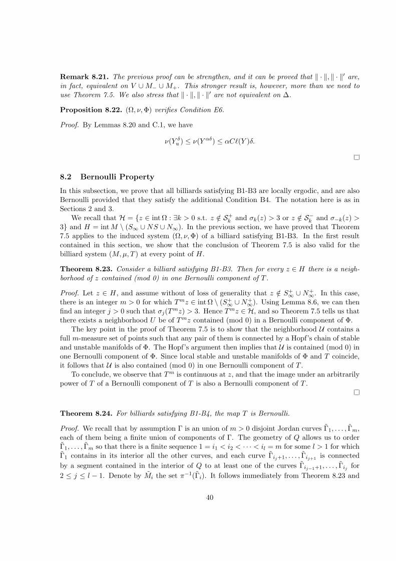
Remark 8.21. The previous proof can be strengthen, and it can be proved that ‖ · ‖, ‖ · ‖′ are,in fact, equivalent on V ∪M− ∪M+. This stronger result is, however, more than we need touse Theorem 7.5. We also stress that ‖ · ‖, ‖ · ‖′ are not equivalent on ∆.

Proposition 8.22. (Ω, ν,Φ) verifies Condition E6.

Proof. By Lemmas 8.20 and C.1, we have

ν(Y δu ) ≤ ν(Y αδ) ≤ αC`(Y )δ.

8.2 Bernoulli Property

In this subsection, we prove that all billiards satisfying B1-B3 are locally ergodic, and are alsoBernoulli provided that they satisfy the additional Condition B4. The notation here is as inSections 2 and 3.

We recall that H = z ∈ intΩ : ∃k > 0 s.t. z /∈ S+k and σk(z) > 3 or z /∈ S−k and σ−k(z) >

3 and H = intM \ (S∞ ∪NS ∪N∞). In the previous section, we have proved that Theorem7.5 applies to the induced system (Ω, ν,Φ) of a billiard satisfying B1-B3. In the first resultcontained in this section, we show that the conclusion of Theorem 7.5 is also valid for thebilliard system (M,µ, T ) at every point of H.

Theorem 8.23. Consider a billiard satisfying B1-B3. Then for every z ∈ H there is a neigh-borhood of z contained (mod 0) in one Bernoulli component of T .

Proof. Let z ∈ H, and assume without of loss of generality that z /∈ S+∞ ∪ N+

∞. In this case,there is an integer m > 0 for which Tmz ∈ intΩ \ (S+

∞ ∪N+∞). Using Lemma 8.6, we can then

find an integer j > 0 such that σj(Tmz) > 3. Hence Tmz ∈ H, and so Theorem 7.5 tells us thatthere exists a neighborhood U be of Tmz contained (mod 0) in a Bernoulli component of Φ.

The key point in the proof of Theorem 7.5 is to show that the neighborhood U contains afull m-measure set of points such that any pair of them is connected by a Hopf’s chain of stableand unstable manifolds of Φ. The Hopf’s argument then implies that U is contained (mod 0) inone Bernoulli component of Φ. Since local stable and unstable manifolds of Φ and T coincide,it follows that U is also contained (mod 0) in one Bernoulli component of T .

To conclude, we observe that Tm is continuous at z, and that the image under an arbitrarilypower of T of a Bernoulli component of T is also a Bernoulli component of T .

Theorem 8.24. For billiards satisfying B1-B4, the map T is Bernoulli.

Proof. We recall that by assumption Γ is an union of m > 0 disjoint Jordan curves Γ1, . . . , Γm,each of them being a finite union of components of Γ. The geometry of Q allows us to orderΓ1, . . . , Γm so that there is a finite sequence 1 = i1 < i2 < · · · < il = m for some l > 1 for whichΓ1 contains in its interior all the other curves, and each curve Γij+1, . . . , Γij+1 is connectedby a segment contained in the interior of Q to at least one of the curves Γij−1+1, . . . , Γij for2 ≤ j ≤ l − 1. Denote by Mi the set π−1(Γi). It follows immediately from Theorem 8.23 and

40

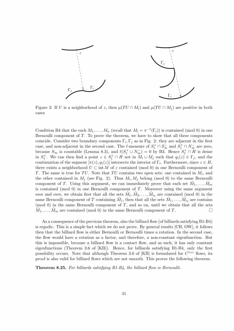
ΓiΓj

zz

Γi

Γj

Figure 2: If U is a neighborhood of z, then µ(TU ∩Mi) and µ(TU ∩Mj) are positive in bothcases

Condition B4 that the each M1, . . . ,Mn (recall that Mi = π−1(Γi)) is contained (mod 0) in oneBernoulli component of T . To prove the theorem, we have to show that all these componentscoincide. Consider two boundary components Γi,Γj as in Fig. 2: they are adjacent in the firstcase, and non-adjacent in the second case. The `-measure of S+

1 ∩ S−∞ and S+1 ∩N−

∞ are zero,because S∞ is countable (Lemma 8.3), and `(S+

1 ∪ N−∞) = 0 by B3. Hence S+

1 ∩ H is densein S+

1 . We can then find a point z ∈ S+1 ∩ H not in Mi ∪Mj such that q1(z) ∈ Γj , and the

continuation of the segment [π(z), q1(z)] intersects the interior of Γi. Furthermore, since z ∈ H,there exists a neighborhood U ⊂ intM of z contained (mod 0) in one Bernoulli component ofT . The same is true for TU . Note that TU contains two open sets: one contained in Mi, andthe other contained in Mj (see Fig. 2). Thus Mi,Mj belong (mod 0) to the same Bernoullicomponent of T . Using this argument, we can immediately prove that each set M1, . . . , Mm

is contained (mod 0) in one Bernoulli component of T . Moreover using the same argumentover and over, we obtain first that all the sets M1, M2, . . . , Mi2 are contained (mod 0) in thesame Bernoulli component of T containing M1, then that all the sets M1, . . . , Mi3 are contains(mod 0) in the same Bernoulli component of T , and so on, until we obtain that all the setsM1, . . . , Mm are contained (mod 0) in the same Bernoulli component of T .

As a consequence of the previous theorem, also the billiard flow (of billiards satisfying B1-B4)is ergodic. This is a simple fact which we do not prove. By general results [CH, OW], it followsthen that the billiard flow is either Bernoulli or Bernoulli times a rotation. In the second case,the flow would have a rotation as a factor, and therefore, a non-constant eigenfunction. Butthis is impossible, because a billiard flow is a contact flow, and as such, it has only constanteigenfunctions (Theorem 3.6 of [KB]). Hence, for billiards satisfying B1-B4, only the firstpossibility occurs. Note that although Theorem 3.6 of [KB] is formulated for C1+ε flows, itsproof is also valid for billiard flows which are not smooth. This proves the following theorem.

Theorem 8.25. For billiards satisfying B1-B4, the billiard flow is Bernoulli.

41

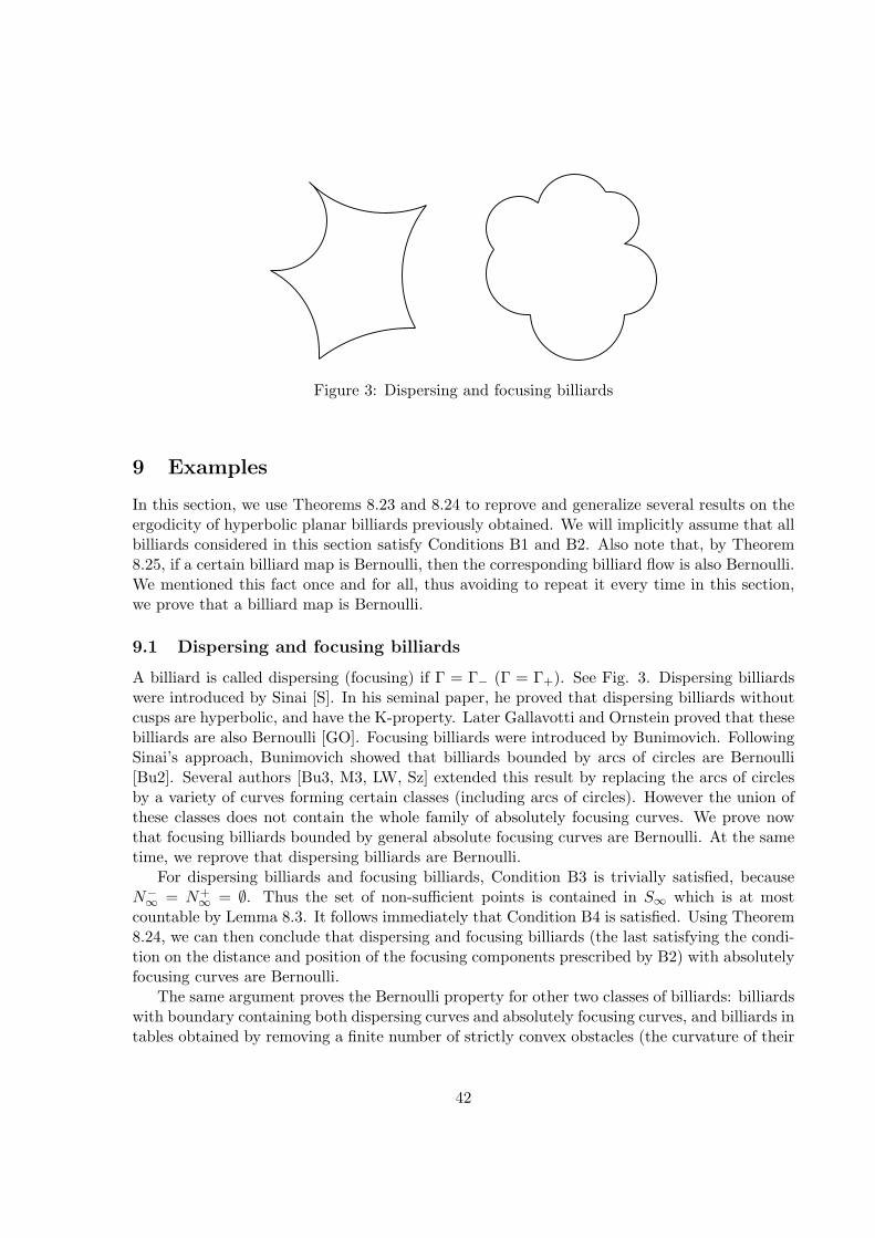
Figure 3: Dispersing and focusing billiards

9 Examples

In this section, we use Theorems 8.23 and 8.24 to reprove and generalize several results on theergodicity of hyperbolic planar billiards previously obtained. We will implicitly assume that allbilliards considered in this section satisfy Conditions B1 and B2. Also note that, by Theorem8.25, if a certain billiard map is Bernoulli, then the corresponding billiard flow is also Bernoulli.We mentioned this fact once and for all, thus avoiding to repeat it every time in this section,we prove that a billiard map is Bernoulli.

9.1 Dispersing and focusing billiards

A billiard is called dispersing (focusing) if Γ = Γ− (Γ = Γ+). See Fig. 3. Dispersing billiardswere introduced by Sinai [S]. In his seminal paper, he proved that dispersing billiards withoutcusps are hyperbolic, and have the K-property. Later Gallavotti and Ornstein proved that thesebilliards are also Bernoulli [GO]. Focusing billiards were introduced by Bunimovich. FollowingSinai’s approach, Bunimovich showed that billiards bounded by arcs of circles are Bernoulli[Bu2]. Several authors [Bu3, M3, LW, Sz] extended this result by replacing the arcs of circlesby a variety of curves forming certain classes (including arcs of circles). However the union ofthese classes does not contain the whole family of absolutely focusing curves. We prove nowthat focusing billiards bounded by general absolute focusing curves are Bernoulli. At the sametime, we reprove that dispersing billiards are Bernoulli.

For dispersing billiards and focusing billiards, Condition B3 is trivially satisfied, becauseN−∞ = N+

∞ = ∅. Thus the set of non-sufficient points is contained in S∞ which is at mostcountable by Lemma 8.3. It follows immediately that Condition B4 is satisfied. Using Theorem8.24, we can then conclude that dispersing and focusing billiards (the last satisfying the condi-tion on the distance and position of the focusing components prescribed by B2) with absolutelyfocusing curves are Bernoulli.

The same argument proves the Bernoulli property for other two classes of billiards: billiardswith boundary containing both dispersing curves and absolutely focusing curves, and billiards intables obtained by removing a finite number of strictly convex obstacles (the curvature of their

42

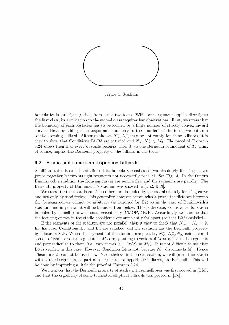
Figure 4: Stadium

boundaries is strictly negative) from a flat two-torus. While our argument applies directly tothe first class, its application to the second class requires few observations. First, we stress thatthe boundary of each obstacles has to be formed by a finite number of strictly convex inwardcurves. Next by adding a “transparent” boundary to the “border” of the torus, we obtain asemi-dispersing billiard. Although the set N−

∞, N+∞ may be not empty for these billiards, it is

easy to show that Conditions B1-B3 are satisfied and N−∞, N

+∞ ⊂ M0. The proof of Theorem

8.24 shows then that every obstacle belongs (mod 0) to one Bernoulli component of T . This,of course, implies the Bernoulli property of the billiard in the torus.

9.2 Stadia and some semidispersing billiards

A billiard table is called a stadium if its boundary consists of two absolutely focusing curvesjoined together by two straight segments not necessarily parallel. See Fig. 4. In the famousBunimovich’s stadium, the focusing curves are semicircles, and the segments are parallel. TheBernoulli property of Bunimovich’s stadium was showed in [Bu2, Bu3].

We stress that the stadia considered here are bounded by general absolutely focusing curveand not only by semicircles. This generality however comes with a price: the distance betweenthe focusing curves cannot be arbitrary (as required by B2) as in the case of Bunimovich’sstadium, and in general, it will be bounded from below. This is the case, for instance, for stadiabounded by semiellipses with small eccentricity [CMOP, MOP]. Accordingly, we assume thatthe focusing curves in the stadia considered are sufficiently far apart (so that B2 is satisfied).

If the segments of the stadium are not parallel, then it easy to check that N−∞ = N+

∞ = ∅.In this case, Conditions B3 and B4 are satisfied and the stadium has the Bernoulli propertyby Theorem 8.24. When the segments of the stadium are parallel, N−

∞, N+∞, N∞ coincide and

consist of two horizontal segments in M corresponding to vectors of M attached to the segmentsand perpendicular to them (i.e., two curves θ = π/2 in M0). It is not difficult to see thatB3 is verified in this case. However Condition B4 is not, because N∞ disconnects M0. HenceTheorem 8.24 cannot be used now. Nevertheless, in the next section, we will prove that stadiawith parallel segments, as part of a large class of hyperbolic billiards, are Bernoulli. This willbe done by improving a little the proof of Theorem 8.24.

We mention that the Bernoulli property of stadia with semiellipses was first proved in [DM],and that the ergodicity of some truncated elliptical billiards was proved in [De].

43

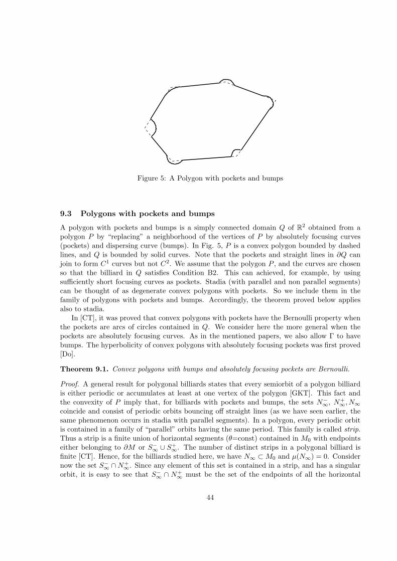
Figure 5: A Polygon with pockets and bumps

9.3 Polygons with pockets and bumps

A polygon with pockets and bumps is a simply connected domain Q of R2 obtained from apolygon P by “replacing” a neighborhood of the vertices of P by absolutely focusing curves(pockets) and dispersing curve (bumps). In Fig. 5, P is a convex polygon bounded by dashedlines, and Q is bounded by solid curves. Note that the pockets and straight lines in ∂Q canjoin to form C1 curves but not C2. We assume that the polygon P , and the curves are chosenso that the billiard in Q satisfies Condition B2. This can achieved, for example, by usingsufficiently short focusing curves as pockets. Stadia (with parallel and non parallel segments)can be thought of as degenerate convex polygons with pockets. So we include them in thefamily of polygons with pockets and bumps. Accordingly, the theorem proved below appliesalso to stadia.

In [CT], it was proved that convex polygons with pockets have the Bernoulli property whenthe pockets are arcs of circles contained in Q. We consider here the more general when thepockets are absolutely focusing curves. As in the mentioned papers, we also allow Γ to havebumps. The hyperbolicity of convex polygons with absolutely focusing pockets was first proved[Do].

Theorem 9.1. Convex polygons with bumps and absolutely focusing pockets are Bernoulli.

Proof. A general result for polygonal billiards states that every semiorbit of a polygon billiardis either periodic or accumulates at least at one vertex of the polygon [GKT]. This fact andthe convexity of P imply that, for billiards with pockets and bumps, the sets N−

∞, N+∞, N∞

coincide and consist of periodic orbits bouncing off straight lines (as we have seen earlier, thesame phenomenon occurs in stadia with parallel segments). In a polygon, every periodic orbitis contained in a family of “parallel” orbits having the same period. This family is called strip.Thus a strip is a finite union of horizontal segments (θ=const) contained in M0 with endpointseither belonging to ∂M or S−∞ ∪ S+

∞. The number of distinct strips in a polygonal billiard isfinite [CT]. Hence, for the billiards studied here, we have N∞ ⊂M0 and µ(N∞) = 0. Considernow the set S−∞ ∩N+

∞. Since any element of this set is contained in a strip, and has a singularorbit, it is easy to see that S−∞ ∩ N+

∞ must be the set of the endpoints of all the horizontal

44

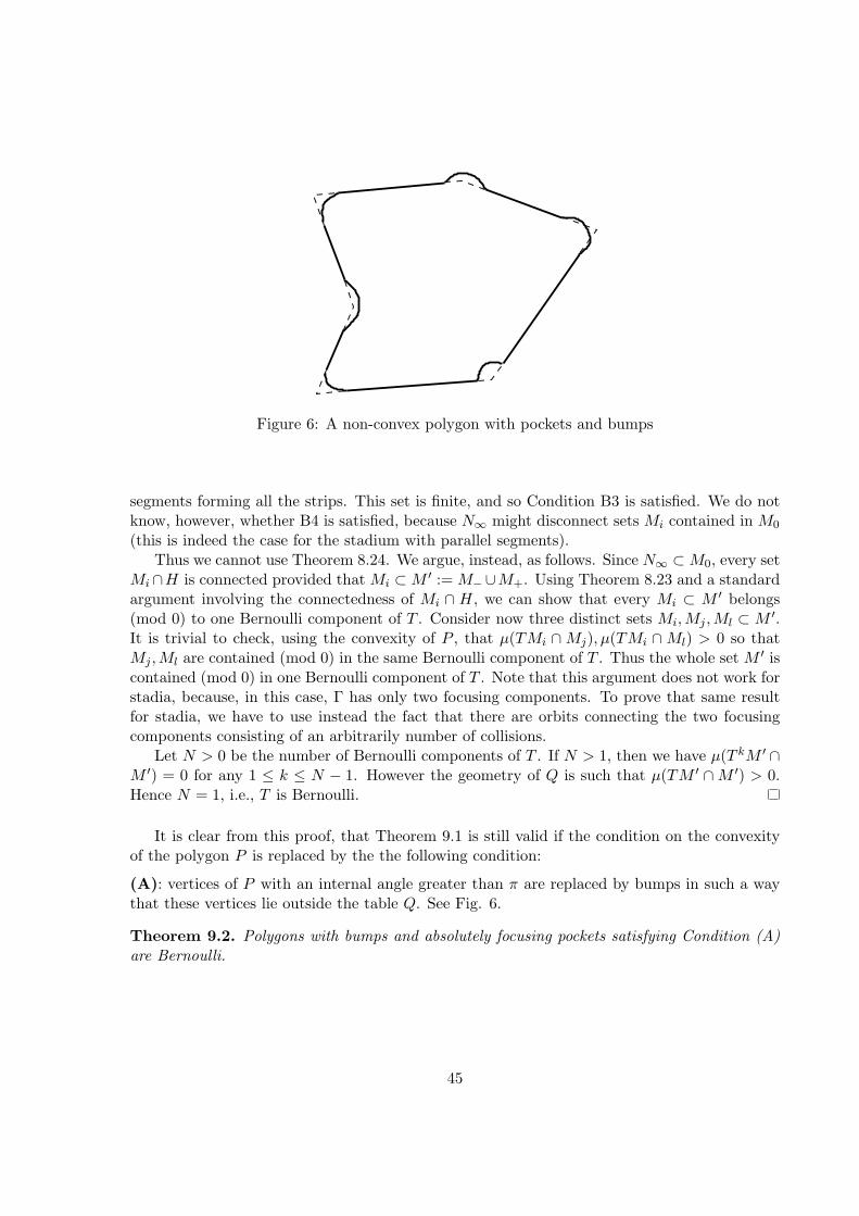
Figure 6: A non-convex polygon with pockets and bumps

segments forming all the strips. This set is finite, and so Condition B3 is satisfied. We do notknow, however, whether B4 is satisfied, because N∞ might disconnect sets Mi contained in M0

(this is indeed the case for the stadium with parallel segments).Thus we cannot use Theorem 8.24. We argue, instead, as follows. Since N∞ ⊂M0, every set

Mi∩H is connected provided that Mi ⊂M ′ := M−∪M+. Using Theorem 8.23 and a standardargument involving the connectedness of Mi ∩ H, we can show that every Mi ⊂ M ′ belongs(mod 0) to one Bernoulli component of T . Consider now three distinct sets Mi,Mj ,Ml ⊂ M ′.It is trivial to check, using the convexity of P , that µ(TMi ∩Mj), µ(TMi ∩Ml) > 0 so thatMj ,Ml are contained (mod 0) in the same Bernoulli component of T . Thus the whole set M ′ iscontained (mod 0) in one Bernoulli component of T . Note that this argument does not work forstadia, because, in this case, Γ has only two focusing components. To prove that same resultfor stadia, we have to use instead the fact that there are orbits connecting the two focusingcomponents consisting of an arbitrarily number of collisions.

Let N > 0 be the number of Bernoulli components of T . If N > 1, then we have µ(T kM ′ ∩M ′) = 0 for any 1 ≤ k ≤ N − 1. However the geometry of Q is such that µ(TM ′ ∩M ′) > 0.Hence N = 1, i.e., T is Bernoulli.

It is clear from this proof, that Theorem 9.1 is still valid if the condition on the convexityof the polygon P is replaced by the the following condition:

(A): vertices of P with an internal angle greater than π are replaced by bumps in such a waythat these vertices lie outside the table Q. See Fig. 6.

Theorem 9.2. Polygons with bumps and absolutely focusing pockets satisfying Condition (A)are Bernoulli.

45

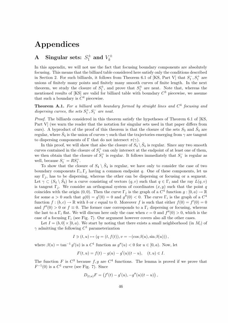
Appendices

A Singular sets: S±1 and V ±k

In this appendix, we will not use the fact that focusing boundary components are absolutelyfocusing. This means that the billiard table considered here satisfy only the conditions describedin Section 2. For such billiards, it follows from Theorem 6.1 of [KS, Part V] that S−1 , S

+1 are

unions of finitely many points and finitely many smooth curves of finite length. In the nexttheorem, we study the closure of S±1 , and prove that S±1 are neat. Note that, whereas thementioned results of [KS] are valid for billiard table with boundary C3 piecewise, we assumethat such a boundary is C4 piecewise.

Theorem A.1. For a billiard with boundary formed by straight lines and C4 focusing anddispersing curves, the sets S+

1 , S−1 are neat.

Proof. The billiards considered in this theorem satisfy the hypotheses of Theorem 6.1 of [KS,Part V] (we warn the reader that the notation for singular sets used in that paper differs fromours). A byproduct of the proof of this theorem is that the closure of the sets S3 and S4 areregular, where S4 is the union of curves γ such that the trajectories emerging from γ are tangentto dispersing components of Γ that do not intersect π(γ).

In this proof, we will show that also the closure of S4 \ S4 is regular. Since any two smoothcurves contained in the closure of S+

1 can only intersect at the endpoint of at least one of them,we then obtain that the closure of S+

1 is regular. It follows immediately that S−1 is regular aswell, because S−1 = RS+

1 .To show that the closure of S4 \ S4 is regular, we have only to consider the case of two

boundary components Γi,Γj having a common endpoint q. One of these components, let ussay Γj , has to be dispersing, whereas the other can be dispersing or focusing or a segment.Let γ ⊂ (S4 \ S4) be a curve consisting of vectors (q, v) such that q ∈ Γi and the ray L(q, v)is tangent Γj . We consider an orthogonal system of coordinates (x, y) such that the point qcoincides with the origin (0, 0). Then the curve Γj is the graph of a C4 function g : [0, a) → Rfor some a > 0 such that g(0) = g′(0) = 0 and g′′(0) < 0. The curve Γi is the graph of a C4

function f : (b, c) → R with b or c equal to 0. Moreover f is such that either f(0) = f ′(0) = 0and f ′′(0) > 0 or f ≡ 0. The former case corresponds to a Γi dispersing or focusing, whereasthe last to a Γi flat. We will discuss here only the case when c = 0 and f ′′(0) > 0, which is thecase of a focusing Γi (see Fig. 7). Our argument however covers also all the other cases.

Let I = (b, 0]× [0, a). We start by noting that there exists a small neighborhood (in Mi) ofγ admitting the following C1 parameterization

I 3 (t, u) 7→ (q = (t, f(t)), v = −(cosβ(u), sinβ(u))) ,

where β(u) = tan−1 g′(u) is a C1 function as g′′(u) < 0 for u ∈ [0, a). Now, let

F (t, u) = f(t)− g(u)− g′(u)(t− u), (t, u) ∈ I.

The function F is C3 because f, g are C4 functions. The lemma is proved if we prove thatF−1(0) is a C1 curve (see Fig. 7). Since

D(t,u)F =(f ′(t)− g′(u),−g′′(u)(t− u)

),

46

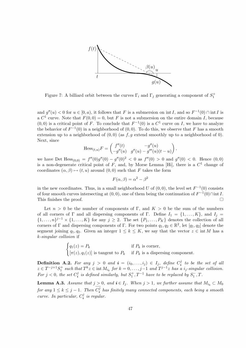
u

f(t)

t

β(u)

g(u)

Figure 7: A billiard orbit between the curves Γi and Γj generating a component of S+1

and g′′(u) < 0 for u ∈ [0, a), it follows that F is a submersion on int I, and so F−1(0) ∩ int I isa C1 curve. Note that F (0, 0) = 0, but F is not a submersion on the entire domain I, because(0, 0) is a critical point of F . To conclude that F−1(0) is a C1 curve on I, we have to analyzethe behavior of F−1(0) in a neighborhood of (0, 0). To do this, we observe that F has a smoothextension up to a neighborhood of (0, 0) (as f, g extend smoothly up to a neighborhood of 0).Next, since

Hess(t,u)F =(f ′′(t) −g′′(u)−g′′(u) g′′(u)− g′′′(u)(t− u)

),

we have Det Hess(0,0) = f ′′(0)g′′(0) − g′′(0)2 < 0 as f ′′(0) > 0 and g′′(0) < 0. Hence (0, 0)is a non-degenerate critical point of F , and, by Morse Lemma [Hi], there is a C1 change ofcoordinates (α, β) 7→ (t, u) around (0, 0) such that F takes the form

F (α, β) = α2 − β2

in the new coordinates. Thus, in a small neighborhood U of (0, 0), the level set F−1(0) consistsof four smooth curves intersecting at (0, 0), one of them being the continuation of F−1(0)∩ int I.This finishes the proof.

Let n > 0 be the number of components of Γ, and K > 0 be the sum of the numbersof all corners of Γ and all dispersing components of Γ. Define I1 = 1, . . . ,K, and Ij =1, . . . , nj−1 × 1, . . . ,K for any j ≥ 2. The set P1, . . . , PK denotes the collection of allcorners of Γ and dispersing components of Γ. For two points q1, q2 ∈ R2, let [q1, q2] denote thesegment joining q1, q2. Given an integer 1 ≤ k ≤ K, we say that the vector z ∈ intM has ak-singular collision if

q1(z) = Pk if Pk is corner,[π(z), q1(z)] is tangent to Pk if Pk is a dispersing component.

Definition A.2. For any j > 0 and i = (i0, . . . , ij) ∈ Ij, define Cji to be the set of all

z ∈ T−j+1S+1 such that T kz ∈ intMik for k = 0, . . . , j−1 and T j−1z has a ij-singular collision.

For j < 0, the set Cji is defined similarly, but S+

1 , T−1 have to be replaced by S−1 , T .

Lemma A.3. Assume that j > 0, and i ∈ Ij. When j > 1, we further assume that Mik ⊂M0

for any 1 ≤ k ≤ j − 1. Then Cji has finitely many connected components, each being a smooth

curve. In particular, Cji is regular.

47

Proof. By the hypotheses of the lemma, the set Cji coincides with the set C1

i ′with a proper i ′,

associated to the billiard obtained by unfolding the original billiard table along the trajectoriesof Cj

i . The set C1i ′

is not connected when there is an “obstacle” which splits the orbits ofelements of C1

i ′. Since there might be only finitely many such obstacles (Γ has finitely many

components), C1i ′

must have finitely many connected components. By Theorem 6.1 of [KS,Part V], these components are smooth, and Theorem A.1 tells us that their closure is smoothas well. This finishes the proof, we observe, as it is easy to check, that the closures of any twoconnected components of C1

i ′do not intersect.

Lemma A.4. All the indexes j, j′ and i, i′ involved in the following propositions are assumedto satisfy the hypothesis of Lemma A.3. We have

1. for any j, j′ > 0, i ∈ Ij , i ∈ Ij′ such that (j, i) 6= (j′, i′), we have Cji ∩ C

j′

i′⊂ ∂Cj

i ∪ ∂Cj′

i′,

2. for any j > 0, i ∈ Ij, and any connected component ξ of Cji , there exist 0 < j′ ≤ j, i′ ∈ Ij′

with i′0 = i0 such that ∂ξ ⊂ Cj′

i′∪ ∂M ,

3. for any j > 0, the set (∪1≤k≤j ∪i∈IkCk

i ) ∪ ∂M is connected.

Proof. The proof of the first statement is an easy consequence of the definition of Cji . The proof

of the second and third propositions are essentially the same: it is enough to note that if theclosure of a connected component of Cj

i does not intersect any connected component (distinctthan itself) of Cj′

i ′with 0 < j′ ≤ j, then it reaches ∂M .

We recall the definitions of several sets given in Section 4. Let V +1 = S+

1 ∩M0, and defineinductively V +

k = (T−1V +k−1∩M0)∪V +

1 for k > 1. We similarly define V −n by replacing S+

1 , T−1

by S−1 , T . The sets V ±k consist of elements of M0 having at most k − 1 consecutive collisions

with Γ0 before hitting a corner of Γ or having a tangential collision at Γ−. Let Vk = V −k ∪ V +

k ,and ∂M0 = ∂M ∩M0.

Corollary A.5. In the following propositions, the unions are restricted to i’s satisfying thehypothesis of Lemma A.3. We have

1. S+1 = ∪i∈I1C

1i , and S+

1 is neat,

2. V +k = ∪1≤m≤k ∪i∈Im Cm

i (where the union has to be further restricted to i’s satisfyingMi0 ⊂M0), and V +

k is neat,

3. T−1V +k = ∪2≤m≤k ∪i∈Im Cm

i , and T−1V +k is neat.

Similar propositions are valid for the sets S−1 , V−k , TV

−k .

Proof. It follows immediately from the definition of the sets involved and Lemmas A.3 andA.4.

48

B Singular sets: S±kThis appendix contains a result (Theorem B.4) which is crucial to prove the regularity of S±kfor any k > 0. Surprisingly we do not know whether the same result is valid for S±k for anyk > 0 (Theorem A.1 tells us that this is the case for k = 1). This is one of the reasons forintroducing the induced system (Ω, ν,Φ).

Definition B.1. Let N > 0. A smooth component of S+N if γ is a smooth compact curve γ

which is the closure of a connected component of Cji ∩S

+N 6= ∅ for some 1 ≤ j ≤ N(2n− 1) and

i ∈ Ij.

Lemma B.2. Consider a billiard satisfying B1. Let N be a non-negative integers, and γ1, γ2

be smooth components of S+N . Then either γ1 = γ2 or γ1 ∩ γ2 ⊂ ∂γ1 ∪ ∂γ2. A similar result is

valid for smooth components of S−N .

Proof. By the time-reversing symmetry of billiard systems, it is enough to prove the lemmafor smooth components of S+

N . Let j1, j2 be the integers as in the Definition B.1 referring toγ1, γ2, respectively. Suppose that γ1 ∩ γ2 6= ∅. Let z ∈ γ1 ∩ γ2, and assume without loss ofgenerality that z ∈ int γ1. In this case, we have j1 ≤ j2. It is easy to see that if j1 = j2 andγ1, γ2 are generated by the same corner or dispersing component of Γ, then γ1 = γ2, otherwisez ∈ ∂γ2.

Lemma B.3. Consider a billiard satisfying B1 and B2. Let N1, N2 be two non-negative inte-gers, and γ1, γ2 be smooth components of S+

N1and S−N2

, respectively. Then γ1 ∩ γ2 is finite.

Proof. For i = 1, 2, let Γi be the component of Γ for which π(γi) ⊂ Γi. If Γ1 6= Γ2, then weobtain trivially that γ1 ∩ γ2 ⊂ ∂γ1 ∩ ∂γ2, and so γ1 ∩ γ2 is finite. In the rest of this proof, wetherefore consider the case Γ1 = Γ2, and study separately the two possibilities: γ1, γ2 ∈ M+

and γ1, γ2 ∈M− ∪∆.So suppose now that Γ1 is a focusing component of Γ. The corresponding phase space is M1.

We will show, in this case, that Tzγ1 ⊂ intC ′(z) and Tzγ2 ⊂ intC(z) for any z ∈ γ1 ∩ γ2. Thisfact will implies that γ1, γ2 are transversal, and therefore finite because smooth componentsare by definition compact. To carried out our plan, we further split this part of the proofin the study of several cases, i.e, when γ1 ⊂ R+

N1(γ2 ⊂ R−

N2), and when γ1 ⊂ S+

N1\ R+

N1

(γ2 ⊂ S−N2\ R−

N2). Before starting analyzing these cases, we observe that if z ∈ γ1 ∩ γ2, then

z /∈ S2. So let γ1 ⊂ R+N1

. By the definition of a smooth component, and that the restriction ofT to M1 ∩ T−1M1 is a diffeomorphism (see Section 5.3), we can find an integer 0 < n1 ≤ N1

such that Tn1γ1 is a smooth compact curve of S1 ∩ M1 (the “vertical” boundary of M1).It follows that if 0 6= u ∈ Tzγ1, then DzT

n1u = a∂/∂θ(Tn1z) for some a 6= 0. We recallthat, in the construction of C in Section 5.3, the vector ∂/∂θ(y) generates the edge of C(y)which gets mapped strictly inside the next cone. Thus by the invariance of C, we obtain thatu ∈ intC ′(z), i.e, Tzγ1 ⊂ intC ′(z). Similarly one can show that Tzγ2 ⊂ intC(z) when γ2 ⊂ R−

N2.

We consider now the case γ1 ⊂ S+N1\ R+

N1. Let I1 3 t 7→ γ1(t) be a regular parameterization

of γ1 where I1 is a closed interval. As before, there exists an integer 0 ≤ n1 < N1 such thatξ1 := Tn1 int γ1 is a smooth open curve contained in S+

1 with a regular parameterization given

49

by int I1 3 t 7→ ξ1(t) := Tn1γ1(t). Note that this time, we can only claim that Tn1 is adiffeomorphism on int γ1. Hence τ+(ξ1, ξ′1(t)) is equal to the length of the segment connectingπ(ξ1) and the corner or dispersing component of Γ generating γ1. Let γ1 be the curve on M1

which is the last iterate of γ1 before this leavesM1. This curve is smooth and compact because Tis a diffeomorphism on M1 ∩T−1M1. Let t 7→ γ1(t) denote the obvious regular parametrizationof γ1. It is not difficult to see that Condition B2 and the invariance of C imply

τ+(γ1(t), γ′1(t)) > τ+i + τ , t ∈ int I1. (19)

Suppose now that z = γ1(t1) for some t1 ∈ I1. Since z /∈ S2, passing to the limit as t → t1 in(19) , we obtain

τ+(γ1(t1), γ′1(t1)) > τ+i + τ .

This implies that γ′1(t1) ∈ intC ′(γ1(t1)), and, using the invariance of C, we obtain γ′1(t1) ∈intC ′(z), i.e., Tzγ1 ⊂ intC ′(z). Similarly one can prove that Tzγ2 ⊂ intC(z) when γ2 ⊂S−N2

\ R−N2

.To finish the proof, we have to analyze the case γ1, γ2 ∈ M− ∪ ∆. For i = 1, 2, let Ii 3

t 7→ γi(t) be a parameterization of γi as described above. A similar argument to the one aboveshows that γ′1(t) ∈ intC ′(γ1(t)) for every t ∈ int I1, and γ′2(t) ∈ intC(γ2(t)) for every t ∈ int I2.In coordinates (s, θ), we have intC(z) = (s′, θ′) : s′θ′ < 0 for z ∈ M− ∪ ∆, and so γ1, γ2

are, respectively, strictly increasing and decreasing. It follows that γ1 ∩ γ2 can contain at mostone element. We note that, as an bonus, we obtain that γ′1(t) ∈ C ′(γ1(t)) for t ∈ ∂I1 andγ′2(t) ∈ C(γ2(t)) for t ∈ ∂I2.

Theorem B.4. Consider a billiard satisfying B1 and B2. Let j > 0, and γ be a smoothcomponent of S−j such that int γ ∩ S+

1 = ∅. Then Φ int γ is smooth. A similar conclusion isvalid if we replace S−j ,S

+1 ,Φ by S+

j ,S−1 ,Φ

−1.

Proof. It is enough to prove the theorem only for images of Φ; by the time-symmetry of thebilliard dynamics, the theorem extends automatically to images of Φ−1.

To prove the theorem, we argue as follows. First of all, note that there is a 0 < k ≤ 2n− 1such that Φ int γ = T kγ. Let Γi,Γj be the boundary components of Γ, not necessarily distinct,such that γ ∈Mi and T k int γ ∈Mj . Our goal is to show that T k int γ is smooth.

If we consider an orthogonal system of coordinates (x, y), then the curve Γi is the graph ofa C3 function f : [0, a] → R for some a > 0 such that f(0) = 0. Note that the conditions thatwe have imposed on the components of Γ (see Section 2) imply that if f ′′ is zero at some point,then f is linear, i.e., Γi is a straight line. For any t ∈ [0, a], the value α(t) denotes the anglethat the x-axis forms with the tangent of the graph of f at (t, f(t)), i.e., f ′(t) = tanα(t). Weconsider the following C1 parameterization of γ

t 7→ γ(t) := ((t, f(t)), θ(t)) ∈Mi, t ∈ [0, a′]

where θ(t) is the angle formed by the vector γ(t) with the oriented tangent of Γi at (t, f(t)),and 0 < a′ ≤ a. See Fig. 8.

For any t ∈ [0, a′], let L(t) be the ray which is the continuation of the vector γ(t). Denoteby β(t) the angle that x-axis forms with L(t), and let b(t) = tanβ(t). The functions β and bare C1 on [0, a′]. We may assume without loss of generality that b(0) = 0.

50

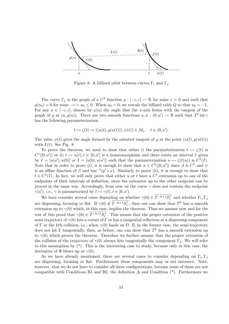
θ(t)

t α(t)

ψ(t)

u

f(t)g(u)

L(t)

Figure 8: A billiard orbit between curves Γi and Γj

The curve Γj is the graph of a C3 function g : [−c, c] → R for some c > 0 and such thatg(u0) = 0 for some −c < u0 ≤ 0. When u0 < 0, we rescale the billiard table Q so that u0 = −1.For any u ∈ [−c, c], denote by ϕ(u) the angle that the x-axis forms with the tangent of thegraph of g at (u, g(u)). There are two smooth functions u, ψ : (0, a′) → R such that T k int γhas the following parameterization

t 7→ ζ(t) := ((u(t), g(u(t))), ψ(t)) ∈Mj , t ∈ (0, a′).

The value ψ(t) gives the angle formed by the oriented tangent of g at the point (u(t), g(u(t)))with L(t). See Fig. 8.

To prove the theorem, we need to show that either i) the parameterization t 7→ ζ(t) isC1([0, a′]) or ii) t 7→ u(t), t ∈ [0, a′] is a homeomorphism and there exists an interval I givenby I = [u(a′), u(0)] or I = [u(0), u(a′)] such that the parameterization u 7→ ζ(t(u)) is C1(I).Note that in order to prove (i), it is enough to show that u ∈ C1([0, a′]) since β is C1 and ψis an affine function of β and tan−1(g′ u). Similarly to prove (ii), it is enough to show thatt ∈ C1(I). In fact, we will only prove that either u or t have a C1 extension up to one of theendpoints of their intervals of definition, since the extension up to the other endpoint can beproved in the same way. Accordingly, from now on the curve γ does not contain the endpointγ(a′), i.e., γ is parameterized by t 7→ γ(t), t ∈ [0, a′).

We have consider several cases depending on whether γ(0) ∈ T−k+1S+1 and whether Γi,Γj

are dispersing, focusing or flat. If γ(0) /∈ T−k+1S+1 , then one can show that T k has a smooth

extension up to γ(0) which, in this case, implies the theorem. Thus we assume now and for therest of this proof that γ(0) ∈ T−k+1S+

1 . This means that the proper extension of the positivesemi-trajectory of γ(0) hits a corner of Γ or has a tangential reflection at a dispersing componentof Γ at the kth collision, i.e., when γ(0) lands on Ω. If, in the former case, the semi-trajectorydoes not hit Γ tangentially, then, as before, one can show that T k has a smooth extension upto γ(0) which proves the theorem. Therefore we further assume that the proper extension ofthe collision of the trajectory of γ(0) always hits tangentially the component Γj . We will referto this assumption by (*). This is the interesting case to study, because only in this case, thederivative of Φ blows up at γ(0).

As we have already mentioned, there are several cases to consider depending on Γi,Γj

are dispersing, focusing or flat. Furthermore these components may or not intersect. Note,however, that we do not have to consider all these configurations, because some of them are notcompatible with Conditions B1 and B2, the definition ∆ and Condition (*). Furthermore we

51

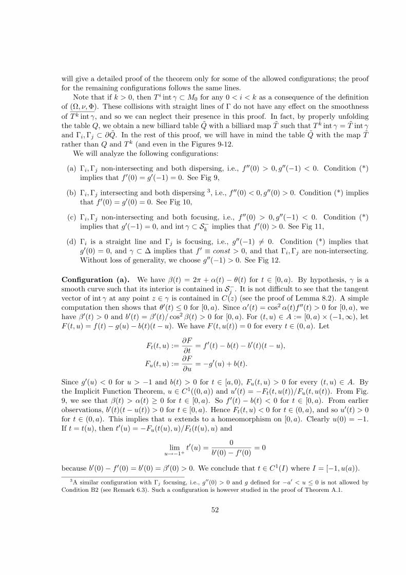
will give a detailed proof of the theorem only for some of the allowed configurations; the prooffor the remaining configurations follows the same lines.

Note that if k > 0, then T i int γ ⊂ M0 for any 0 < i < k as a consequence of the definitionof (Ω, ν,Φ). These collisions with straight lines of Γ do not have any effect on the smoothnessof T k int γ, and so we can neglect their presence in this proof. In fact, by properly unfoldingthe table Q, we obtain a new billiard table Q with a billiard map T such that T k int γ = T int γand Γi,Γj ⊂ ∂Q. In the rest of this proof, we will have in mind the table Q with the map Trather than Q and T k (and even in the Figures 9-12.

We will analyze the following configurations:

(a) Γi,Γj non-intersecting and both dispersing, i.e., f ′′(0) > 0, g′′(−1) < 0. Condition (*)implies that f ′(0) = g′(−1) = 0. See Fig 9,

(b) Γi,Γj intersecting and both dispersing 3, i.e., f ′′(0) < 0, g′′(0) > 0. Condition (*) impliesthat f ′(0) = g′(0) = 0. See Fig 10,

(c) Γi,Γj non-intersecting and both focusing, i.e., f ′′(0) > 0, g′′(−1) < 0. Condition (*)implies that g′(−1) = 0, and int γ ⊂ S−k implies that f ′(0) > 0. See Fig 11,

(d) Γi is a straight line and Γj is focusing, i.e., g′′(−1) 6= 0. Condition (*) implies thatg′(0) = 0, and γ ⊂ ∆ implies that f ′ ≡ const > 0, and that Γi,Γj are non-intersecting.Without loss of generality, we choose g′′(−1) > 0. See Fig 12.

Configuration (a). We have β(t) = 2π + α(t) − θ(t) for t ∈ [0, a). By hypothesis, γ is asmooth curve such that its interior is contained in S−j . It is not difficult to see that the tangentvector of int γ at any point z ∈ γ is contained in C(z) (see the proof of Lemma 8.2). A simplecomputation then shows that θ′(t) ≤ 0 for [0, a). Since α′(t) = cos2 α(t)f ′′(t) > 0 for [0, a), wehave β′(t) > 0 and b′(t) = β′(t)/ cos2 β(t) > 0 for [0, a). For (t, u) ∈ A := [0, a) × (−1,∞), letF (t, u) = f(t)− g(u)− b(t)(t− u). We have F (t, u(t)) = 0 for every t ∈ (0, a). Let

Ft(t, u) :=∂F

∂t= f ′(t)− b(t)− b′(t)(t− u),

Fu(t, u) :=∂F

∂u= −g′(u) + b(t).

Since g′(u) < 0 for u > −1 and b(t) > 0 for t ∈ [a, 0), Fu(t, u) > 0 for every (t, u) ∈ A. Bythe Implicit Function Theorem, u ∈ C1((0, a)) and u′(t) = −Ft(t, u(t))/Fu(t, u(t)). From Fig.9, we see that β(t) > α(t) ≥ 0 for t ∈ [0, a). So f ′(t) − b(t) < 0 for t ∈ [0, a). From earlierobservations, b′(t)(t− u(t)) > 0 for t ∈ [0, a). Hence Ft(t, u) < 0 for t ∈ (0, a), and so u′(t) > 0for t ∈ (0, a). This implies that u extends to a homeomorphism on [0, a). Clearly u(0) = −1.If t = t(u), then t′(u) = −Fu(t(u), u)/Ft(t(u), u) and

limu→−1+

t′(u) =0

b′(0)− f ′(0)= 0

because b′(0)− f ′(0) = b′(0) = β′(0) > 0. We conclude that t ∈ C1(I) where I = [−1, u(a)).3A similar configuration with Γj focusing, i.e., g′′(0) > 0 and g defined for −a′ < u ≤ 0 is not allowed by

Condition B2 (see Remark 6.3). Such a configuration is however studied in the proof of Theorem A.1.

52

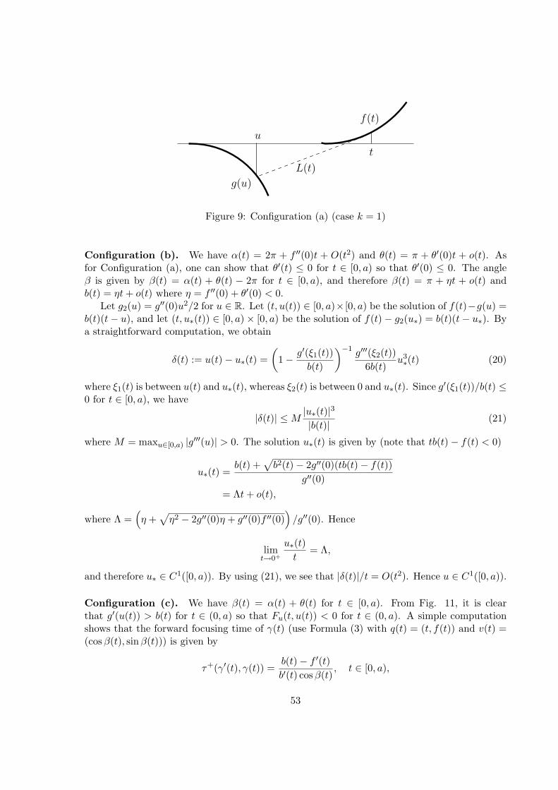
f(t)

g(u)

L(t)

u

t

Figure 9: Configuration (a) (case k = 1)

Configuration (b). We have α(t) = 2π + f ′′(0)t + O(t2) and θ(t) = π + θ′(0)t + o(t). Asfor Configuration (a), one can show that θ′(t) ≤ 0 for t ∈ [0, a) so that θ′(0) ≤ 0. The angleβ is given by β(t) = α(t) + θ(t) − 2π for t ∈ [0, a), and therefore β(t) = π + ηt + o(t) andb(t) = ηt+ o(t) where η = f ′′(0) + θ′(0) < 0.

Let g2(u) = g′′(0)u2/2 for u ∈ R. Let (t, u(t)) ∈ [0, a)× [0, a) be the solution of f(t)−g(u) =b(t)(t− u), and let (t, u∗(t)) ∈ [0, a)× [0, a) be the solution of f(t)− g2(u∗) = b(t)(t− u∗). Bya straightforward computation, we obtain

δ(t) := u(t)− u∗(t) =(

1− g′(ξ1(t))b(t)

)−1 g′′′(ξ2(t))6b(t)

u3∗(t) (20)

where ξ1(t) is between u(t) and u∗(t), whereas ξ2(t) is between 0 and u∗(t). Since g′(ξ1(t))/b(t) ≤0 for t ∈ [0, a), we have

|δ(t)| ≤M|u∗(t)|3

|b(t)|(21)

where M = maxu∈[0,a) |g′′′(u)| > 0. The solution u∗(t) is given by (note that tb(t)− f(t) < 0)

u∗(t) =b(t) +

√b2(t)− 2g′′(0)(tb(t)− f(t))

g′′(0)= Λt+ o(t),

where Λ =(η +

√η2 − 2g′′(0)η + g′′(0)f ′′(0)

)/g′′(0). Hence

limt→0+

u∗(t)t

= Λ,

and therefore u∗ ∈ C1([0, a)). By using (21), we see that |δ(t)|/t = O(t2). Hence u ∈ C1([0, a)).

Configuration (c). We have β(t) = α(t) + θ(t) for t ∈ [0, a). From Fig. 11, it is clearthat g′(u(t)) > b(t) for t ∈ (0, a) so that Fu(t, u(t)) < 0 for t ∈ (0, a). A simple computationshows that the forward focusing time of γ(t) (use Formula (3) with q(t) = (t, f(t)) and v(t) =(cosβ(t), sinβ(t))) is given by

τ+(γ′(t), γ(t)) =b(t)− f ′(t)b′(t) cosβ(t)

, t ∈ [0, a),

53

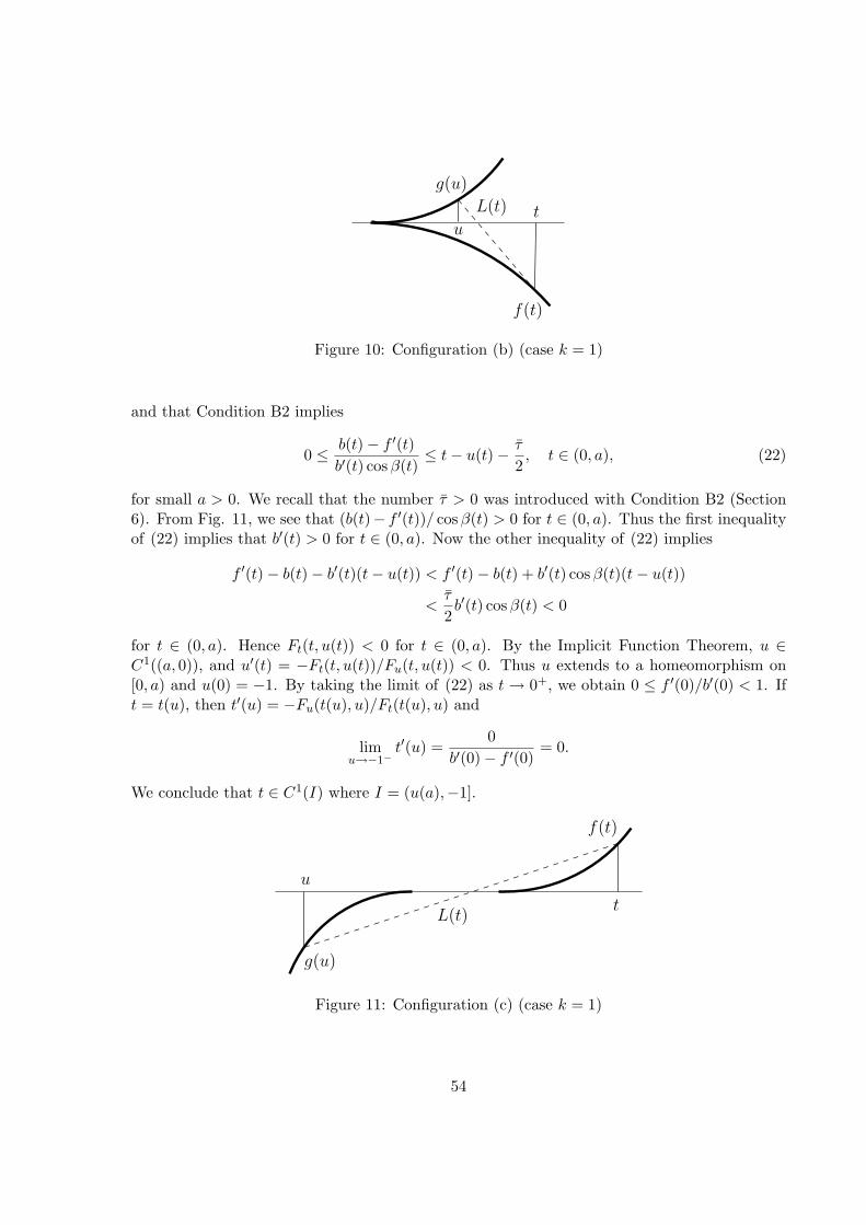
f(t)

tu

g(u)

L(t)

Figure 10: Configuration (b) (case k = 1)

and that Condition B2 implies

0 ≤ b(t)− f ′(t)b′(t) cosβ(t)

≤ t− u(t)− τ

2, t ∈ (0, a), (22)

for small a > 0. We recall that the number τ > 0 was introduced with Condition B2 (Section6). From Fig. 11, we see that (b(t)− f ′(t))/ cosβ(t) > 0 for t ∈ (0, a). Thus the first inequalityof (22) implies that b′(t) > 0 for t ∈ (0, a). Now the other inequality of (22) implies

f ′(t)− b(t)− b′(t)(t− u(t)) < f ′(t)− b(t) + b′(t) cosβ(t)(t− u(t))

<τ

2b′(t) cosβ(t) < 0

for t ∈ (0, a). Hence Ft(t, u(t)) < 0 for t ∈ (0, a). By the Implicit Function Theorem, u ∈C1((a, 0)), and u′(t) = −Ft(t, u(t))/Fu(t, u(t)) < 0. Thus u extends to a homeomorphism on[0, a) and u(0) = −1. By taking the limit of (22) as t→ 0+, we obtain 0 ≤ f ′(0)/b′(0) < 1. Ift = t(u), then t′(u) = −Fu(t(u), u)/Ft(t(u), u) and

limu→−1−

t′(u) =0

b′(0)− f ′(0)= 0.

We conclude that t ∈ C1(I) where I = (u(a),−1].

f(t)

tL(t)

u

g(u)

Figure 11: Configuration (c) (case k = 1)

54

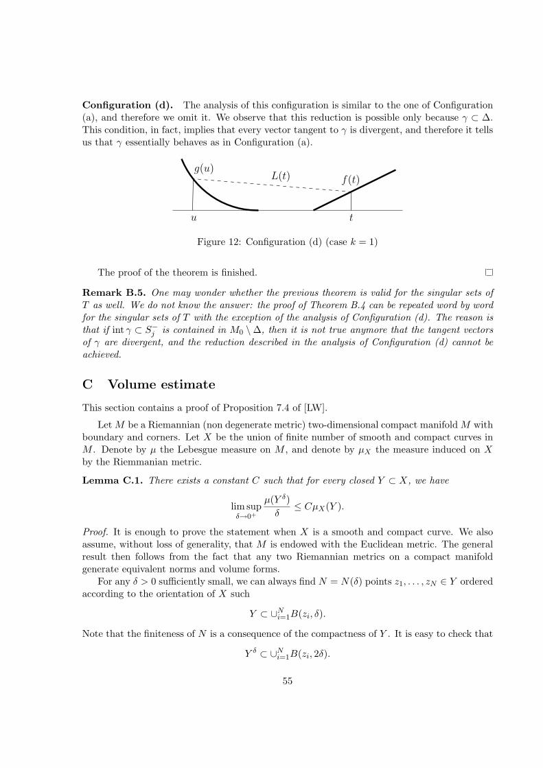
Configuration (d). The analysis of this configuration is similar to the one of Configuration(a), and therefore we omit it. We observe that this reduction is possible only because γ ⊂ ∆.This condition, in fact, implies that every vector tangent to γ is divergent, and therefore it tellsus that γ essentially behaves as in Configuration (a).

tu

g(u)f(t)L(t)

Figure 12: Configuration (d) (case k = 1)

The proof of the theorem is finished.

Remark B.5. One may wonder whether the previous theorem is valid for the singular sets ofT as well. We do not know the answer: the proof of Theorem B.4 can be repeated word by wordfor the singular sets of T with the exception of the analysis of Configuration (d). The reason isthat if int γ ⊂ S−j is contained in M0 \∆, then it is not true anymore that the tangent vectorsof γ are divergent, and the reduction described in the analysis of Configuration (d) cannot beachieved.

C Volume estimate

This section contains a proof of Proposition 7.4 of [LW].

Let M be a Riemannian (non degenerate metric) two-dimensional compact manifold M withboundary and corners. Let X be the union of finite number of smooth and compact curves inM . Denote by µ the Lebesgue measure on M , and denote by µX the measure induced on Xby the Riemmanian metric.

Lemma C.1. There exists a constant C such that for every closed Y ⊂ X, we have

lim supδ→0+

µ(Y δ)δ

≤ CµX(Y ).

Proof. It is enough to prove the statement when X is a smooth and compact curve. We alsoassume, without loss of generality, that M is endowed with the Euclidean metric. The generalresult then follows from the fact that any two Riemannian metrics on a compact manifoldgenerate equivalent norms and volume forms.

For any δ > 0 sufficiently small, we can always find N = N(δ) points z1, . . . , zN ∈ Y orderedaccording to the orientation of X such

Y ⊂ ∪Ni=1B(zi, δ).

Note that the finiteness of N is a consequence of the compactness of Y . It is easy to check that

Y δ ⊂ ∪Ni=1B(zi, 2δ).

55

We claim that there exists an index set J ⊂ 1, . . . , N such if l,m ∈ J and l 6= m, then

B(zl, 2δ) ∩B(zm, 2δ) = ∅,

and∪N

i=1B(zi, 2δ) ⊂ ∪j∈JB(zj , 6δ).

We give here a sketch of the proof of this claim, which, in fact, follows from a more general result(see for instance Lemma 6.8 of [F]). The construction of the subcover indexed by J is doneinductively. Pick as the first element of the subcover any element of the original cover. Supposethat we have already chosen the first k − 1 elements. The next element is chosen among theremaining balls of the original cover which do not intersect the k − 1 already chosen elements.The process ends when no such ball remains. Now it is easy to check that the subcover justconstructed has the required properties.

For sufficiently small r > 0, the measure of a ball of radius r is not larger than cr2 for someconstant c > 0 independent on the ball. Thus

µ(Y δ) ≤∑j∈J

µ(B(zj , 6δ)) ≤ 9cδ∑j∈J

diam(B(zi, 2δ)).

Since ∑j∈J

diam(B(zi, 2δ)) ≤ µX(X ∩⋃j∈J

B(zj , 2δ)) ≤ µX(X ∩N⋃

i=1

B(zi, 2δ)),

and

limδ→0+

µX(X ∩N⋃

i=1

B(zi, 2δ)) = µX(Y ),

we obtainlim supδ→0+

∑j∈J

diam(B(zi, 2δ)) ≤ µX(Y ).

We conclude that

lim supδ→0+

µ(Y δ)δ

≤ 9cµX(Y ).

Remark C.2. The previous proof works also for degenerate metrics provided that the measureof a ball of radius r is not greater than cr2 where c is a constant independent of the ballconsidered.

References

[Bu1] L. A. Bunimovich, Billiards that are close to scattering billiards, (Russian) Mat. Sb.(N.S.) 94(136) (1974), 49-73.

[Bu2] L. A. Bunimovich, On ergodic properties of nowhere dispersing billiards, Comm. Math.Phys. 65 (1979), 295-312.

56

[Bu3] L. A. Bunimovich, A theorem on ergodicity of two-dimensional hyperbolic billiards,Comm. Math. Phys. 130 (1990), 599-621.

[Bu4] L. A. Bunimovich, On absolutely focusing mirrors, Ergodic theory and related topics,III (Gustrow, 1990), Springer (1992), 62-82.

[BS] L. A. Bunimovich and Ya. G. Sinai, The fundamental theorem of the theory of scat-tering billiards, Mat. Sb. (N.S.) 90(132) (1973), 415-431.

[BSC] L. A. Bunimovich, Ya. G. Sinai and N. I. Chernov, Statistical properties of two-dimensional hyperbolic billiards, Russ. Math. Surv. 46 (1991), 47-106.

[BCST] P. Balint, N. Chernov, D. Szasz, I. P. Toth, Multi-dimensional semi-dispersing bil-liards: singularities and the fundamental theorem, Ann. Henri Poincare 3 (2002),451-482.

[C] N. I. Chernov, Local ergodicity of hyperbolic systems with singularities, Functional.Anal. Appl. 27 (1993), 51-54.

[CH] N. I. Chernov and C. Haskell, Nonuniformly hyperbolic K-systems are Bernoulli, Er-god. Th. & Dynam. Sys. 16 (1996), 19-44.

[CM1] N. I. Chernov and R. Markarian, Entropy of non-uniformly hyperbolic plane billiards,Bol. Soc. Bras. Mat. 23 (1992), 121-135.

[CM2] N. I. Chernov and R. Markarian, Introduction to the ergodic theory of chaotic billiards,Second Edition - Revised and Enlarged, Publicacoes Matematicas, IMPA, Rio deJaneiro, 2003.

[CT] N. I. Chernov and S. Troubetzkoy, Ergodicity of billiards in polygons with pockets,Nonlinearity 11 (1998), 1095-1102.

[CFS] I. P. Cornfeld, S. V. Fomin and Ya. G. Sinai, Ergodic Theory, Springer, Berlin 1982.

[CMOP] E. Canale, R. Markarian, S. Oliffson Khamporst and S. Pinto de Carvalho, A lowerbound for chaos on the elliptical stadium, Physica D 115 (1998), 189-202.

[De] G. Del Magno, Ergodicity of a class of truncated elliptical billiard, Nonlinearity 14(2001), 1761-1786.

[DM] G. Del Magno and R. Markarian, Bernoulli Elliptical Stadia, Comm. Math. Phys. 233(2003), 211-230.

[Do] V. Donnay, Using Integrability to Produce chaos: Billiards with Positive Entropy,Comm. Math. Phys. 141 (1991), 225-257.

[F] K. Falconer, Fractal geometry, John Wiley & Sons Ltd., 1990.

[GO] G. Gallavotti and D. S. Ornstein, Billiards and Bernoulli Schemes, Comm. Math.Phys. 38 (1974), 83-101.

57

[GKT] G. Gal’perin, T. Kruger and S. Troubetzkoy, Local instability of orbits in polygonaland polyhedral billiards, Comm. Math. Phys. 169 (1995), 463-473.

[Ha] B. Halpern, Strange billiard tables, Trans. Amer. Math. Soc. 232 (1977), 297-305.

[Hi] M. Hirsch, Differential Topology, Graduate Texts in Mathematics 33, Springer-Verlag,New York-Heidelberg, 1976.

[Ho] E. Hopf, Statistik der geodatischen Linien in Mannigfaltigkeiten negativer Krummung,Ber. Verh. Sachs. Akad. Wiss. Leipzig 91 (1939), 261-304.

[KB] A. Katok and K. Burns, Infinitesimal Lyapunov functions, invariant cone familiesand stochastic properties of smooth dynamical systems, Ergod. Th. & Dynam. Sys. 14(1994), 757-785.

[KS] A. Katok and J.-M. Strelcyn, Invariant manifolds, entropy and billiards; smooth mapswith singularities, Lect. Notes Math. 1222, Springer, New York, 1986.

[KMS] S. Kerckhoff, H. Masur and J. Smillie, Ergodicity of billiard flows and quadratic dif-ferentials, Ann. Math. 124 (1986), 293-311.

[KSS] A. Kramli, N. Simanyi and D. Szasz, A “transversal” fundamental theorem for semi-dispersing billiards, (see also Erratum) Comm. Math. Phys. 129 (1990), 535-560.

[La] V. F. Lazutkin, On the existence of caustics for the billiard ball problem in a convexdomain, Math. USSR Izv. 7 (1973), 185-215.

[Li] C. Liverani, Decay of correlations, Ann. of Math. 142 (1995), 239-301.

[LW] C. Liverani and M. Wojtkowski, Ergodicity in Hamiltonian Systems, Dynamics re-ported, Dynam. Report. Expositions Dynam. Systems (N.S.) 4 Springer, Berlin (1995),130-202.

[M1] R. Markarian, Billiards with Pesin region of measure one, Comm. Math. Phys. 118(1988), 87-97.

[M2] R. Markarian, The fundamental theorem of Sinaı-Chernov for dynamical systems withsingularities, Dynamical systems (Santiago, 1990), Pitman Res. Notes Math. Ser. 285,Longman Sci. Tech., Harlow (1993), 131-158.

[M3] R. Markarian, New ergodic billiards: exact results, Nonlinearity 6 (1993), 819-841.

[M4] R. Markarian, Non-uniformly hyperbolic billiards, Ann. Fac. Sci. Toulouse Math. 3(1994), 223-257.

[MOP] R. Markarian, S. Oliffson Khamporst and S. Pinto de Carvalho, Chaotic Properties ofthe Elliptical Stadium, Comm. Math. Phys. 174 (1996), 661-679.

[OW] D. S. Ornstein and B. Weiss, On the Bernoulli nature of systems with hyperbolicstructure, Ergod. Th. & Dynam. Sys. 18 (1998), 441-456.

58

[P] Ya. B. Pesin, Characteristic Lyapunov exponents and smooth ergodic theory, Russ.Math. Surv. 32 (1977), 55-114.

[S] Ya. G. Sinai, Dynamical systems with elastic reflections. Ergodic properties of dispers-ing billiards, Russ. Math. Surv. 25 (1970), 137-189.

[SC] Ya. G. Sinai and N. I. Chernov, Ergodic properties of some systems of two-dimensionaldisks and three-dimensional balls, Russ. Math. Surv. 42 (1987), 181-207.

[Sz] D. Szasz, On the K-property of some planar hyperbolic billiards, Comm. Math. Phys.145 (1992), 595-604.

[T] S. Tabachnikov, Billiards, Panoramas et Syntheses 1, Societe Mathematique deFrance, 1995.

[W1] M. Wojtkowski, Invariant families of cones and Lyapunov exponents, Ergod. Th. &Dynam. Sys. 5 (1985), 145-161.

[W2] M. Wojtkowski, Principles for the design of billiards with nonvanishing Lyapunovexponents, Comm. Math. Phys. 105 (1986), 391-414.

[W3] M. Wojtkowski, Two applications of Jacobi fields to the billiard ball problem, J. Dif-ferential Geom. 40 (1994), 155-164.

59