On the application of the Jensen wake model using a ...orbit.dtu.dk/files/122284235/On_the_application_of_the_Jensen_wake... · Pena Diaz, A., Réthoré, P-E., & van der Laan, P

General rights Copyright and moral rights for the publications made accessible in the public portal are retained by the authors and/or other copyright owners and it is a condition of accessing publications that users recognise and abide by the legal requirements associated with these rights.

• Users may download and print one copy of any publication from the public portal for the purpose of private study or research. • You may not further distribute the material or use it for any profit-making activity or commercial gain • You may freely distribute the URL identifying the publication in the public portal

If you believe that this document breaches copyright please contact us providing details, and we will remove access to the work immediately and investigate your claim.

Downloaded from orbit.dtu.dk on: Oct 09, 2018

On the application of the Jensen wake model using a turbulence-dependent wakedecay coefficient: the Sexbierum case

Pena Diaz, Alfredo; Réthoré, Pierre-Elouan; van der Laan, Paul

Published in:Wind Energy

Link to article, DOI:10.1002/we.1863

Publication date:2016

Document VersionPublisher's PDF, also known as Version of record

Link back to DTU Orbit

Citation (APA):Pena Diaz, A., Réthoré, P-E., & van der Laan, P. (2016). On the application of the Jensen wake model using aturbulence-dependent wake decay coefficient: the Sexbierum case. Wind Energy, 19, 763–776. DOI:10.1002/we.1863

http://dx.doi.org/10.1002/we.1863

http://orbit.dtu.dk/en/publications/on-the-application-of-the-jensen-wake-model-using-a-turbulencedependent-wake-decay-coefficient-the-sexbierum-case(9abcbbb8-a864-43b3-b653-1ed1c813dc95).html

WIND ENERGYWind Energ. 2016; 19:763–776

Published online 7 May 2015 in Wiley Online Library (wileyonlinelibrary.com). DOI: 10.1002/we.1863

RESEARCH ARTICLE

On the application of the Jensen wake model using aturbulence-dependent wake decay coefficient: theSexbierum caseAlfredo Peña, Pierre-Elouan Réthoré and M. Paul van der LaanDepartment of Wind Energy, Technical University of Denmark, Risø campus, Roskilde, Denmark

ABSTRACT

We present a methodology to process wind turbine wake simulations, which are closely related to the nature of wake obser-vations and the processing of these to generate the so-called wake cases. The method involves averaging a large number ofwake simulations over a range of wind directions and partly accounts for the uncertainty in the wind direction assumingthat the same follows a Gaussian distribution. Simulations of the single and double wake measurements at the Sexbierumonshore wind farm are performed using a fast engineering wind farm wake model based on the Jensen wake model, a lin-earized computational fluid dynamics wake model by Fuga and a nonlinear computational fluid dynamics wake model thatsolves the Reynolds-averaged Navier–Stokes equations with a modified k-" turbulence model. The best agreement betweenmodels and measurements is found using the Jensen-based wake model with the suggested post-processing. We show thatthe wake decay coefficient of the Jensen wake model must be decreased from the commonly used onshore value of 0.075to 0.038, when applied to the Sexbierum cases, as wake decay is related to the height, roughness and atmospheric stabil-ity and, thus, to turbulence intensity. Based on surface layer relations and assumptions between turbulence intensity andatmospheric stability, we find that at Sexbierum, the atmosphere was probably close to stable, although the stability wasnot observed. We support these assumptions using detailed meteorological observations from the Høvsøre site in Denmark,which is topographically similar to the Sexbierum region. © 2015 The Authors. Wind Energy published by John Wiley &Sons Ltd.

KEYWORDS

atmospheric stability; Sexbierum; turbulence; wake decay coefficient; wake model; wind direction uncertainty

Correspondence

Alfredo Peña, Department of Wind Energy, Technical University of Denmark, Risø campus, Roskilde, Denmark.E-mail: [email protected]

This is an open access article under the terms of the Creative Commons Attribution License, which permits use, distribution andreproduction in any medium, provided the original work is properly cited.

Received 26 May 2014; Revised 30 March 2015; Accepted 16 April 2015

1. INTRODUCTION

The Jensen wake model1 is popular as an engineering wind turbine wake model for the quantification of the reduction ofthe wind speed downstream a wind turbine. This is because it was formulated in the early 1980s when only a few wakemodels were available and is simple, very fast and easy to implement. It is also the base of the Park model2 that wasdeveloped for wind farm calculations for the Wind Atlas Analysis and Application Program (WAsP),3 which is widelyused for the estimation of wind resources. Because of the simplicity of its physical considerations, it is not recognized tobe very accurate at predicting wake losses under specific atmospheric inflow conditions, e.g. when compared with windfarm power and meteorological (met) data averaged over a narrow range of wind speeds and directions. It is neverthelessconsidered to be fairly accurate for predicting wake losses on an annual energy production basis.4

Under such specific conditions, the differences between wake simulations and observations can partly be explainedby the post-processing methodologies used to reproduce the observed results with a set of model simulations, as pointedout by Gaumond et al.5 and Peña et al.6 A ‘wake case’ is usually constructed by narrowing the wind speed to its mostobserved value, often within a range of˙1 m s�1. Then, different ranges of wind directions are considered, e.g.˙5ı,˙10ı

or ˙15ı, and either the observed wind speed or the power deficits are averaged and compared with model simulations.

© 2015 The Authors. Wind Energy published by John Wiley & Sons Ltd. 763

http://creativecommons.org/licenses/by/3.0/

On the application of the Jensen wake model A. Peña, P.-E. Réthoré and M. P. van der Laan

Now, the question that arises is how does one perform the set of model simulations that can be fairly compared withmeasured averages? Until recently, we have only been concerned about the improvement of wake models to account forthe physics of the turbine–atmosphere interaction, e.g. through computational fluid dynamics (CFD). When a new modelor parametrization is developed, it is normally tested against some classic wake cases and generally shows better resultscompared with those from other known and in many cases simpler models (usually, the Jensen wake model is also used forsuch purpose). We do not find this tendency very appealing as some of the simulations are still far from being carried outand post-processed in a similar manner as that used when analyzing the wake observations.

The results from Gaumond et al.5 using a wind farm model based on the Jensen wake model, compared with a numberof standard wake cases at the offshore wind farm Horns Rev I, were as agreeable as those obtained using more advancedwake models, such as that by Fuga,7 which is a linearized CFD model that uses the actuator disc (AD) approach, whenthe post-processing of the results took into account the uncertainty in the wind direction. Gaumond8 actually showed thatfor the single and double wake cases at the Sexbierum wind farm, the results from Fuga’s model and from a CFD solverof the Reynolds-averaged Navier–Stokes (RANS) equations (EllipSyS)9 that uses the AD approach and a standard k-"model are nearly identical; those from the Jensen wake model were not properly post-processed, i.e. the uncertainty in thewind direction was not taken into account, and so the other models seem to a priori achieve better results. Further, a wakedecay coefficient of 0.075 was used with the Jensen wake model, which is the WAsP-recommended value for onshore wakemodeling. Here, we show for the first time

� that this value is nearly two times larger than that obtained for the Sexbierum cases based on a stability-basedparametrization of the wake decay and

� that in case information on stability is lacking, one may use the turbulence intensity (TI) instead, as we show, usinghigh-quality observations from Høvsøre (a similar site to Sexbierum in terms of topography), that turbulence andstability are closely related. The stability-based wake decay approach was already successfully evaluated at the HornsRev I wind farm for a row of 10 turbines and a range of stability conditions.6

But why do we try to improve simple engineering wake models? A number of wind farm flow models have beendeveloped over the years using various physical assumptions. While the Jensen wake model represents one of the mostsimple ‘low-fidelity’ models, it also remains to be popular in the research and industry wind communities because it canbe recalibrated due to its simple wake parametrization. There is always a risk of overfitting while recalibrating models;however, it is important to point out that in wind energy (as an applied science), what ultimately matters is the predictivecapability of the wind farm flow models and not the amount of physics or complexity added to them. Simple engineeringmodels offer the possibility of carrying out simulations orders of magnitude faster than higher fidelity ones, allowing us toperform wind farm analysis and optimization. With the advance of probabilistic methods offering ensemble aggregation ofmodels or even multi-fidelity, low-fidelity models can be combined with higher fidelity ones (an example of the latter isCFD RANS) to perform fast and accurate prediction of annual energy production or even wind farm layout optimization.

Here, we first describe the Jensen wake model and a simple method to estimate the wake decay coefficient based eitheron the height, roughness and atmospheric stability conditions or TI values at a given site (Section 2.1). In Sections 2.2 and2.3, we briefly introduce the two other wake models used in this study, Fuga and a RANS-based model that uses a modifiedk-" turbulence model. Section 3 illustrates the different ways of post-processing the results from the Jensen wake model,e.g. by taking into account the uncertainty in the wind direction. The Sexbierum wake cases are presented in Section 4 andthe results of the comparison between these and the wake models in Section 5, followed by the conclusion and discussion.

2. WAKE MODELSHere, we describe the basics of the three wake models used in this study. For the Jensen wake model, we show the relationsbetween the wake decay coefficient and TI, and the relation between TI and atmospheric stability at the Høvsøre site inDenmark.

2.1. The Jensen wake model

Jensen1 devised a mass-conserving engineering wake model to estimate the hub height wind speed downstream of a turbineat a distance x, u2, when subjected to a hub height inflow wind speed u1 as

1 �u2

u1D

1 �p

1 � Ct

.1C kw x=rr/2

(1)

where Ct is the thrust coefficient, rr is the rotor radius and kw is the wake decay coefficient. Figure 1 illustrates that theJensen wake model assumes the radial speed to be constant within the wake, which expands radially at the rate kw x. Theterm on the left of equation (1) is referred to as the local speed deficit, ı. This model (i.e. the top-hat wake profile shown inFigure 1) is deficient for the far wake but a good approximation in the near wake, e.g. at two rotor diameters downstream.10

Wind Energ. 2016; 19:763–776 © 2015 The Authors. Wind Energy published by John Wiley & Sons Ltd.764DOI: 10.1002/we

A. Peña, P.-E. Réthoré and M. P. van der Laan On the application of the Jensen wake model

Figure 1. The Jensen wake model concept.

−20 −15 −10 −5 0 5 10 15 200.7

0.75

0.8

0.85

0.9

0.95

1

1.05

Figure 2. Wind speed ratio of the Jensen-based wind farm model as a function of the relative wind direction. Two cases are illus-trated: a wake generated by a turbine and observed by a mast (turbine–mast) and a wake generated by a turbine and observed by a

second turbine (turbine–turbine).

2.1.1. Wind farm model.Within a wind farm, the local wakes are superposed to estimate the speed deficit at the nth turbine, ın, and thus, weimplement a quadratic sum of the square of the local speed deficits from the Jensen wake model, each represented with thesubindex i, as suggested by Katic et al.2 and used in WAsP

ın D

nX

iD1

ı2i

!1=2

(2)

The speed at the nth turbine, un, is then given as un D u1 .1 � ın/.When the distance between the local and an upstream turbine is not aligned with the wind’s direction, the local turbine

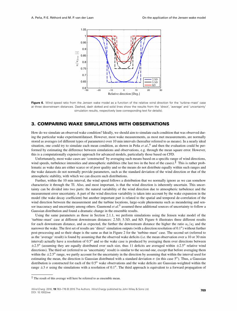
could experience a partial wake interaction. The local speed deficit thus needs to be reduced by a factor that depends onthe crosswise distance between the wake’s center and the local turbine’s center, the local turbine’s radius and the wake’sradius at the downstream position as described by Wan et al.11 This is illustrated in Figure 2, where the wind speed ratiou2=u1 from the wind farm model is plotted as the function of the relative wind direction for two cases: first, assuming oneturbine only and so u2 is ‘observed’ by a point measurement (e.g. a cup anemometer on a met mast) and second, assumingtwo turbines and so u2 is ‘observed’ by the downstream turbine. The simulations are performed at a downstream distanceof 5D, D being the rotor diameter of 30 m using u1 D 8 m s�1, kw D 0.038 and Ct D 0.75 for a wide range of relativewind directions with a resolution of 0.1ı.

Wind Energ. 2016; 19:763–776 © 2015 The Authors. Wind Energy published by John Wiley & Sons Ltd.DOI: 10.1002/we

765


For the ‘turbine–mast’ case, the downstream wind speed sharply decreases at a given angle and so the ratio u2=u1 issimilar to the profile of u2 in Figure 1. Within the wake, u2=u1 is not completely constant (u2 is slightly lower at relativedirections other than 0ı) because the relative downstream distance decreases slightly with increasing relative direction. Forthe ‘turbine–turbine’ case, u2=u1 decreases at larger magnitudes of relative direction (compared with the ‘turbine–mast’case, u2=u1 decreases at � j14ıj) and reaches the maximum deficit at a narrow relative direction range, its size dependingon the diameter of the second turbine. When compared with specific wake cases, results from the Jensen wake model mightlook like those in Figure 2. However, as will be shown in Section 3, such results are misleading, since the characteristics ofthe processing of the observations are not met by these ‘direct’ simulations.

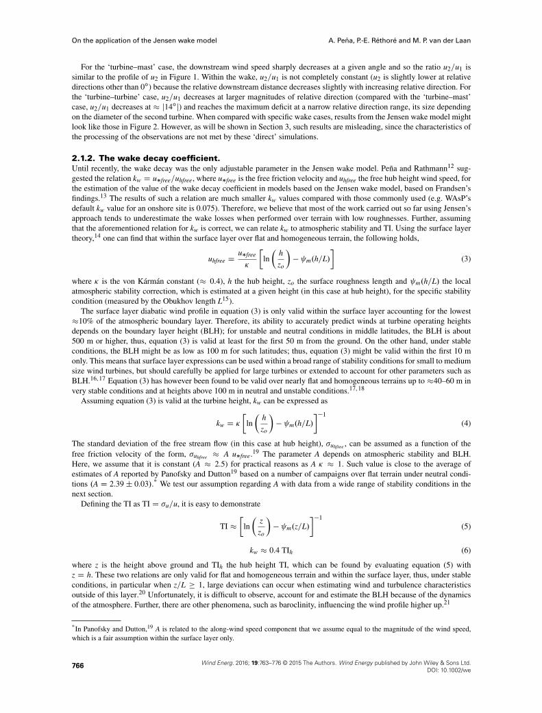
2.1.2. The wake decay coefficient.Until recently, the wake decay was the only adjustable parameter in the Jensen wake model. Peña and Rathmann12 sug-gested the relation kw D u�free=uhfree, where u�free is the free friction velocity and uhfree the free hub height wind speed, forthe estimation of the value of the wake decay coefficient in models based on the Jensen wake model, based on Frandsen’sfindings.13 The results of such a relation are much smaller kw values compared with those commonly used (e.g. WAsP’sdefault kw value for an onshore site is 0.075). Therefore, we believe that most of the work carried out so far using Jensen’sapproach tends to underestimate the wake losses when performed over terrain with low roughnesses. Further, assumingthat the aforementioned relation for kw is correct, we can relate kw to atmospheric stability and TI. Using the surface layertheory,14 one can find that within the surface layer over flat and homogeneous terrain, the following holds,

uhfree Du�free

�

�ln

�h

zo

�� m.h=L/

�(3)

where � is the von Kármán constant (� 0.4), h the hub height, zo the surface roughness length and m.h=L/ the localatmospheric stability correction, which is estimated at a given height (in this case at hub height), for the specific stabilitycondition (measured by the Obukhov length L15).

The surface layer diabatic wind profile in equation (3) is only valid within the surface layer accounting for the lowest�10% of the atmospheric boundary layer. Therefore, its ability to accurately predict winds at turbine operating heightsdepends on the boundary layer height (BLH); for unstable and neutral conditions in middle latitudes, the BLH is about500 m or higher, thus, equation (3) is valid at least for the first 50 m from the ground. On the other hand, under stableconditions, the BLH might be as low as 100 m for such latitudes; thus, equation (3) might be valid within the first 10 monly. This means that surface layer expressions can be used within a broad range of stability conditions for small to mediumsize wind turbines, but should carefully be applied for large turbines or extended to account for other parameters such asBLH.16, 17 Equation (3) has however been found to be valid over nearly flat and homogeneous terrains up to �40–60 m invery stable conditions and at heights above 100 m in neutral and unstable conditions.17, 18

Assuming equation (3) is valid at the turbine height, kw can be expressed as

kw D �

�ln

�h

zo

�� m.h=L/

��1

(4)

The standard deviation of the free stream flow (in this case at hub height), �uhfree , can be assumed as a function of thefree friction velocity of the form, �uhfree � A u�free.19 The parameter A depends on atmospheric stability and BLH.Here, we assume that it is constant (A � 2.5) for practical reasons as A � � 1. Such value is close to the average ofestimates of A reported by Panofsky and Dutton19 based on a number of campaigns over flat terrain under neutral condi-tions .A D 2.39˙ 0.03/.* We test our assumption regarding A with data from a wide range of stability conditions in thenext section.

Defining the TI as TI D �u=u, it is easy to demonstrate

TI �

�ln

�z

zo

�� m.z=L/

��1

(5)

kw � 0.4 TIh (6)

where z is the height above ground and TIh the hub height TI, which can be found by evaluating equation (5) withz D h. These two relations are only valid for flat and homogeneous terrain and within the surface layer, thus, under stableconditions, in particular when z=L � 1, large deviations can occur when estimating wind and turbulence characteristicsoutside of this layer.20 Unfortunately, it is difficult to observe, account for and estimate the BLH because of the dynamicsof the atmosphere. Further, there are other phenomena, such as baroclinity, influencing the wind profile higher up.21

*In Panofsky and Dutton,19 A is related to the along-wind speed component that we assume equal to the magnitude of the wind speed,which is a fair assumption within the surface layer only.



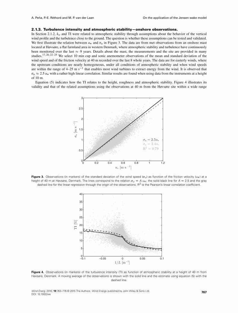
2.1.3. Turbulence intensity and atmospheric stability—onshore observations.In Section 2.1.2, kw and TI were related to atmospheric stability through assumptions about the behavior of the verticalwind profile and the turbulence close to the ground. The question is whether these assumptions can be tested and validated.We first illustrate the relation between u� and �u in Figure 3. The data are from met observations from an onshore mastlocated at Høvsøre, a flat farmland area in western Denmark, where atmospheric stability and turbulence have continuouslybeen monitored over the last � 9 years. Details about the mast, the measurements and the site are provided in manystudies.17, 20, 22–25 We select 10 min cup and sonic anemometer observations of the mean and standard deviation of thewind speed and of the friction velocity at 40 m recorded over the last 8 whole years. The data are for easterly winds, wherethe upstream conditions are nearly homogeneous, under all conditions of atmospheric stability and when wind speedsare within the range of 4–25 m s�1 that enables most wind turbines to extract energy from the wind. It is observed that�u � 2.5 u� with a rather high linear correlation. Similar results are found when using data from the instruments at a heightof 10 m.

Equation (5) indicates how the TI relates to the height, roughness and atmospheric stability. Figure 4 illustrates itsvalidity and that of the related assumptions using the observations at 40 m from the Høvsøre site within a wide range

0 0.2 0.4 0.6 0.8 1 1.20

0.5

1

1.5

2

2.5

3

Figure 3. Observations (in markers) of the standard deviation of the wind speed (�u) as function of the friction velocity (u�) at aheight of 40 m at Høvsøre, Denmark. The lines correspond to the relation �u D A u�; the solid black line for A D 2.5 and the gray

dashed line for the linear regression through the origin of the observations. R2 is the Pearson’s linear correlation coefficient.

−0.1 −0.05 0 0.05 0.10

5

10

15

20

25

30

35

40

Figure 4. Observations (in markers) of the turbulence intensity (TI) as function of atmospheric stability at a height of 40 m fromHøvsøre, Denmark. A moving average of the observations is shown with the solid line and the estimate using equation (5) with the

dashed line.


767


4 6 8 10 12 14 160

5

10

15

20

25

30

35

40

Figure 5. Near-neutral observations (in markers) of turbulence intensity (TI) as a function of wind speed at 40 m at Høvsøre, Denmark.A moving average of the observations is shown with the solid line and the estimate using equation (5) with the dashed line.

of stabilities, �0.1 m�1 � 1=L � 0.1 m�1. On a long-term basis,� the roughness at Høvsøre for easterly upstreamconditions is about 0.015 m (it slightly increases and decreases in summer and winter, respectively) and so we use thisvalue to estimate TI from equation (5). To estimate m, we use the form in Gryning et al.26 for unstable conditions, i.e. m.z=L/ D .3=2/Œ.1C aC a2/=3� �

p3 arctanŒ.1C 2a/=

p3�C �=

p3, where a D .1 � 12z=L/1=3, and m D �4.7z=L

for stable ones. Both forms were previously used at Høvsøre in Gryning et al.26 for evaluating wind profile models.The TI estimation using equation (5) clearly follows the behavior of the moving average of the observations, i.e. higher

and lower TIs are found for unstable and stable conditions, respectively. However, the observations are scattered, partic-ularly under near-neutral and unstable conditions. This is partly due to the scatter of the observations in Figure 3 and tothe accuracy of the diabatic wind profile in equation (3) in predicting the wind speed at this height at Høvsøre. The dif-ferences between the moving average and the TI estimation are partly due to the m forms used and the accuracy of theestimations of L.

The estimate of TI under neutral conditions 1=L � 0 m�1 agrees well with the value from the observations. From thesame data, we select near-neutral conditions (jLj � 1000 m) to analyze the dependency of TI on wind speed. Figure 5illustrates the measurements of TI as function of the wind speed for the height of 40 m, where it is shown a nearly constantbehavior with wind speed as expected from the observations. The average TI for the applied moving window is 12.22%for the height of 40 m, which is nearly the same value as that estimated theoretically using equation (5) with m D 0 andzo D 0.015 m, i.e. 12.68%. Similar agreement is found when using observations from the instruments at the height of 10 m.

2.2. Fuga’s model

Fuga is a linearized flow solver based on the steady-state RANS equations, currently only applicable to flat and homoge-neous terrain. In this model the flow is assumed to be incompressible and lid driven at the chosen inversion height. It usesa simple eddy viscosity turbulence closure and the AD approach. The description of the model and its evaluation with anumber of wind farm datasets can be found in Ott et al.7

2.3. RANS using a modified k-" turbulence model

The AD RANS simulations are carried out in EllipSys3D9 using a modified k-" turbulence model, namely, the k-"-fPmodel.27 The k-"-fP model delays the wake recovery compared with the standard k-" model by introducing a variableeddy viscosity coefficient C�. The variable part of C� is described by a simple scalar function fP that depends on thelocal velocity gradients. Typically, fP is unity in the logarithmic solution, while it is smaller than one for regions with highvelocity gradients. The AD RANS setup including the k-"-fP model has been successfully tested for single wakes,27 doublewakes28 and complete wind farm simulations.29

�Here, long term refers to measurements performed for at least 1 year.



−30 −20 −10 0 10 20 300.6

0.65

0.7

0.75

0.8

0.85

0.9

0.95

1

1.05

Relative direction [Deg.]

2.5D5.5D8D

Figure 6. Wind speed ratio from the Jensen wake model as a function of the relative wind direction for the ‘turbine–mast’ caseat three downstream distances. Dashed, dash dotted and solid lines show the results from the ‘direct’, ‘average’ and ‘uncertainty’

simulation results, respectively (see corresponding text for details).

3. COMPARING WAKE SIMULATIONS WITH OBSERVATIONS

How do we simulate an observed wake condition? Ideally, we should aim to simulate each condition that was observed dur-ing the particular wake experiment/dataset. However, most wake measurements, as most met measurements, are normallystored as averages (of different types of parameters) over 10 min intervals (hereafter referred to as means). In a nearly idealsituation, one could try to simulate each mean condition, as shown in Peña et al.,6 and then the evaluation could be per-formed by estimating the difference between simulations and observations, e.g. through the mean square error. However,this is a computationally expensive approach for advanced models, particularly those based on CFD.

Unfortunately, most wake cases are ‘constructed’ by averaging such means based on a specific range of wind directions,wind speeds, turbulence intensities and atmospheric stabilities (the last two in the best of the cases).� This is rather prob-lematic as wake data are either scarce or of poor quality and so the means do not distribute equally within such ranges andthe wake datasets do not normally provide parameters, such as the standard deviation of the wind direction or that of theatmospheric stability, with which we can discern such distributions.

Further, within the 10 min interval, the wind speed follows a distribution that we normally ignore as we can somehowcharacterize it through the TI. Also, and most important, is that the wind direction is inherently uncertain. This uncer-tainty can be divided into two parts: the natural variability of the wind direction due to atmospheric turbulence and themeasurement error uncertainty. A part of the wind direction variability is taken into account by the wake expansion in themodel (the wake decay coefficient) but another important part is related to the spatial and temporal de-correlation of thewind direction between the measurement and the turbine locations, large-scale phenomena such as meandering and sen-sor inaccuracy and uncertainty among others. Gaumond et al.5 assumed these additional sources of uncertainty to follow aGaussian distribution and found a dramatic change in the ensemble results.

Using the same parameters as those in Section 2.1.1, we perform simulations using the Jensen wake model of the‘turbine–mast’ case at different downstream distances: 2.5D, 5.5D, and 8D. Figure 6 illustrates three different resultsfor each downstream distance, and as expected, the further the downstream distance the higher the ratio u1=u2 and thenarrower the wake. The first set of results are ‘direct’ simulation outputs (with a direction resolution of 0.1ı) without furtherpost-processing and so their shape is the same as that in Figure 2 for the ‘turbine–mast’ case. The second set (referred toas the ‘average’ result) is found by assuming that the observed wake deficits (i.e. the mean observation over a 10 or 30 mininterval) actually have a resolution of 0.5ı and so the wake case is produced by averaging them over directions between˙2.5ı (assuming they are equally distributed over such size, thus 11 deficits are averaged within ˙2.5ı relative winddirections). The third set (referred to as ‘uncertainty’ result) is similar to the second one, except that before averaging themwithin the˙2.5ı range, we partly account for the uncertainty in the direction by assuming that within the interval used forestimating the mean, the direction is Gaussian distributed with a standard deviation � (in this case 5ı). Thus, a Gaussiandistribution is constructed for each of the 0.5ı wake observations and the wake deficits are Gaussian-weighted within therange ˙3 � using the simulations with a resolution of 0.1ı. The third approach is equivalent to a forward propagation of

� The result of this average will here be referred to as ensemble mean.


769


0

50

100

150

200

250

300

350

400

Pow

er [

kW]

4 6 8 10 12 14 16 18 20 220

0.5

1powerthrust

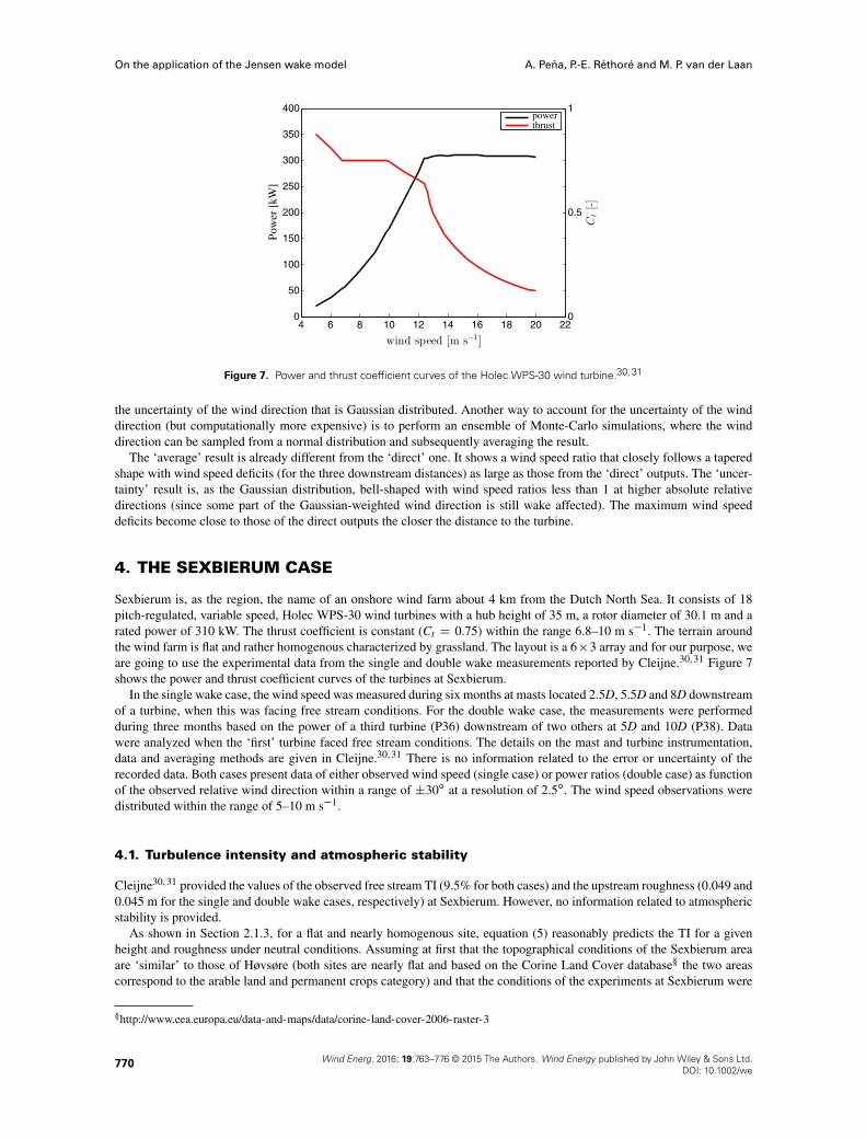
Figure 7. Power and thrust coefficient curves of the Holec WPS-30 wind turbine.30,31

the uncertainty of the wind direction that is Gaussian distributed. Another way to account for the uncertainty of the winddirection (but computationally more expensive) is to perform an ensemble of Monte-Carlo simulations, where the winddirection can be sampled from a normal distribution and subsequently averaging the result.

The ‘average’ result is already different from the ‘direct’ one. It shows a wind speed ratio that closely follows a taperedshape with wind speed deficits (for the three downstream distances) as large as those from the ‘direct’ outputs. The ‘uncer-tainty’ result is, as the Gaussian distribution, bell-shaped with wind speed ratios less than 1 at higher absolute relativedirections (since some part of the Gaussian-weighted wind direction is still wake affected). The maximum wind speeddeficits become close to those of the direct outputs the closer the distance to the turbine.

4. THE SEXBIERUM CASE

Sexbierum is, as the region, the name of an onshore wind farm about 4 km from the Dutch North Sea. It consists of 18pitch-regulated, variable speed, Holec WPS-30 wind turbines with a hub height of 35 m, a rotor diameter of 30.1 m and arated power of 310 kW. The thrust coefficient is constant (Ct D 0.75) within the range 6.8–10 m s�1. The terrain aroundthe wind farm is flat and rather homogenous characterized by grassland. The layout is a 6�3 array and for our purpose, weare going to use the experimental data from the single and double wake measurements reported by Cleijne.30, 31 Figure 7shows the power and thrust coefficient curves of the turbines at Sexbierum.

In the single wake case, the wind speed was measured during six months at masts located 2.5D, 5.5D and 8D downstreamof a turbine, when this was facing free stream conditions. For the double wake case, the measurements were performedduring three months based on the power of a third turbine (P36) downstream of two others at 5D and 10D (P38). Datawere analyzed when the ‘first’ turbine faced free stream conditions. The details on the mast and turbine instrumentation,data and averaging methods are given in Cleijne.30, 31 There is no information related to the error or uncertainty of therecorded data. Both cases present data of either observed wind speed (single case) or power ratios (double case) as functionof the observed relative wind direction within a range of ˙30ı at a resolution of 2.5ı. The wind speed observations weredistributed within the range of 5–10 m s�1.

4.1. Turbulence intensity and atmospheric stability

Cleijne30, 31 provided the values of the observed free stream TI (9.5% for both cases) and the upstream roughness (0.049 and0.045 m for the single and double wake cases, respectively) at Sexbierum. However, no information related to atmosphericstability is provided.

As shown in Section 2.1.3, for a flat and nearly homogenous site, equation (5) reasonably predicts the TI for a givenheight and roughness under neutral conditions. Assuming at first that the topographical conditions of the Sexbierum areaare ‘similar’ to those of Høvsøre (both sites are nearly flat and based on the Corine Land Cover database§ the two areascorrespond to the arable land and permanent crops category) and that the conditions of the experiments at Sexbierum were

§http://www.eea.europa.eu/data-and-maps/data/corine-land-cover-2006-raster-3


http://www.eea.europa.eu/data-and-maps/data/corine-land-cover-2006-raster-3


nearly neutral, the TI is estimated as � 15% using equation (5) for both wake cases, i.e. close to twice the value from theaforementioned reports. A very possible explanation for the mismatch between observed and estimated TI is the influenceof atmospheric stability; from equation (5), the conditions should have to be stable in order to be close to the observed TI.Using the form m D �4.7z=L14 and equation (5) with z D 35 m, TI D 9.5% and zo D 0.049 m, L is estimated to be 42 m.Another possibility is an inaccurate roughness length estimation in Cleijne’s analysis and so there is a range of stabilitiesand roughnesses that can produce the same TI following equation (5). Because of the mismatch and range of possibilities,for the model simulations based on the atmosphere-dependent wake decay coefficient, we use equation (6) to determine kw

from the observed TI at Sexbierum (kw D 0.038/.

5. RESULTS

For both wake cases, we assume the influence from the nearby turbines at Sexbierum to be negligible. So only one and threeturbines are modeled, respectively (this is why the layout of the wind farm is not important). Also, for both cases, simu-lations are performed using a hub height wind speed uh of 8 m s�1, since Cleijne30, 31 reported that the wind speeds weremostly within the range of 7–9 m s�1. Simulations are carried out using the wind farm model described in Section 2.1.1with kw D 0.038, 0.061 and 0.060 (the last two are derived using equation (4) assuming neutral conditions and the rough-ness values from the single and double wake experiments reported earlier, which are close to the default WAsP value) andfor a broad range of relative wind directions (˙60ı) with a resolution of 0.1ı. The observations are reported every 2.5ı,and thus, we post-process the results following the steps described in Section 3 related to the ‘uncertainty’ result. We alsoshow the ‘direct’ results, i.e. those without any post-processing for completeness.

Results using Fuga’s model and RANS using the k-"-fP model are also presented. Fuga’s inputs are uh D 8 m s�1,roughness length (the values from Cleijne30, 31 are used) and inversion height (we choose 200 m, and the model resultsare rather insensitive to this input for the Sexbierum wind farm as the flow is lid driven). For the RANS-based one, weneed uh D 8 m s�1 and TI D

p2=3k=uh D 0.095 and, zo is set so that we obtain the same TI at hub height using

TI D �p

2=3=hln.h=zo/C

1=4�

i, i.e. zo D 0.009 m. Note that C� is 0.03 and cannot be adapted to obtain the desired TI

in the k-"-fP model because the behavior of the fP function changes in an unphysical manner with C�, as discussed invan der Laan et al.27

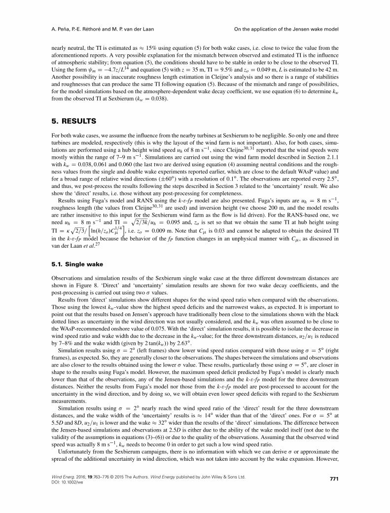
5.1. Single wake

Observations and simulation results of the Sexbierum single wake case at the three different downstream distances areshown in Figure 8. ‘Direct’ and ‘uncertainty’ simulation results are shown for two wake decay coefficients, and thepost-processing is carried out using two � values.

Results from ‘direct’ simulations show different shapes for the wind speed ratio when compared with the observations.Those using the lowest kw-value show the highest speed deficits and the narrowest wakes, as expected. It is important topoint out that the results based on Jensen’s approach have traditionally been close to the simulations shown with the blackdotted lines as uncertainty in the wind direction was not usually considered, and the kw was often assumed to be close tothe WAsP-recommended onshore value of 0.075. With the ‘direct’ simulation results, it is possible to isolate the decrease inwind speed ratio and wake width due to the decrease in the kw-value; for the three downstream distances, u2=u1 is reducedby 7–8% and the wake width (given by 2 tan.kw/) by 2.63ı.

Simulation results using � D 2ı (left frames) show lower wind speed ratios compared with those using � D 5ı (rightframes), as expected. So, they are generally closer to the observations. The shapes between the simulations and observationsare also closer to the results obtained using the lower � value. These results, particularly those using � D 5ı, are closer inshape to the results using Fuga’s model. However, the maximum speed deficit predicted by Fuga’s model is clearly muchlower than that of the observations, any of the Jensen-based simulations and the k-"-fP model for the three downstreamdistances. Neither the results from Fuga’s model nor those from the k-"-fP model are post-processed to account for theuncertainty in the wind direction, and by doing so, we will obtain even lower speed deficits with regard to the Sexbierummeasurements.

Simulation results using � D 2ı nearly reach the wind speed ratio of the ‘direct’ result for the three downstreamdistances, and the wake width of the ‘uncertainty’ results is � 14ı wider than that of the ‘direct’ ones. For � D 5ı at5.5D and 8D, u2=u1 is lower and the wake� 32ı wider than the results of the ‘direct’ simulations. The difference betweenthe Jensen-based simulations and observations at 2.5D is either due to the ability of the wake model itself (not due to thevalidity of the assumptions in equations (3)–(6)) or due to the quality of the observations. Assuming that the observed windspeed was actually 8 m s�1, kw needs to become 0 in order to get such a low wind speed ratio.

Unfortunately from the Sexbierum campaigns, there is no information with which we can derive � or approximate thespread of the additional uncertainty in wind direction, which was not taken into account by the wake expansion. However,


771


−30 −20 −10 0 10 20 300.5

0.6

0.7

0.8

0.9

1

1.1

−30 −20 −10 0 10 20 300.5

0.6

0.7

0.8

0.9

1

1.1

−30 −20 −10 0 10 20 300.5

0.6

0.7

0.8

0.9

1

1.1

−30 −20 −10 0 10 20 300.5

0.6

0.7

0.8

0.9

1

1.1

−30 −20 −10 0 10 20 300.5

0.6

0.7

0.8

0.9

1

1.1

−30 −20 −10 0 10 20 300.5

0.6

0.7

0.8

0.9

1

1.1

Figure 8. Single wake for three downstream distances at Sexbierum: 2.5D (top frames), 5.5D (middle frames) and 8D (bottomframes). Model results are shown with lines and data from Sexbierum with markers. ‘Uncertainty’ results from the Jensen-based

wake model are post-processed using � D 2ı (left frames) and � D 5ı (right frames).

we can use wind direction observations from the Høvsøre site to obtain an idea of the variability of the wind directionwithin a 10 min interval for conditions ‘similar’ to those at Sexbierum.

We select fast measurements (20 Hz) from a sonic anemometer located at 40 m on the Høvsøre mast (the closest tothe hub height at Sexbierum) that are close to the wind conditions at Sexbierum in terms of wind speed, the suggestedatmospheric stability (i.e. L D 42 m that is derived by estimating m.z=L/ from equation (5) using the observed valuesof TI and zo observed at Sexbierum), and TI (derived using equation (5) using the roughness at Høvsøre and the stability,L D 42 m, at Sexbierum). We restrict the analysis to the east sector.



−10 −5 0 5 100

50

100

150

200

250

300

350

400

450

500


NPD

Figure 9. Normalized probability distribution (NPD) of the relative direction observed at Høvsøre for a typical 10 min interval similarto the conditions at Sexbierum. The observations are shown in the histogram with the gray bars, the normal distribution with a solid

black line and with dashed lines the ˙� values (3.5ı/.

Table I. Root mean square error of the wind speed ratio (for the single wake cases)and of the power ratio (for the double wake cases) when comparing model results

with the data from Sexbierum.

Model Single 2.5D Single 5.5D Single 8D Double

Jensen (� D 0ı, kw D 0.038) 0.108 0.059 0.049 0.060Jensen (� D 0ı, kw D 0.060) 0.110 0.048 0.049 0.085Jensen (� D 2ı, kw D 0.038) 0.091 0.035 0.041 0.067Jensen (� D 2ı, kw D 0.060) 0.111 0.045 0.045 0.095Jensen (� D 5ı, kw D 0.038) 0.094 0.039 0.041 0.105Jensen (� D 5ı, kw D 0.060) 0.117 0.052 0.048 0.128Fuga 0.187 0.073 0.056 0.136k-"-fP 0.115 0.053 0.050 0.131

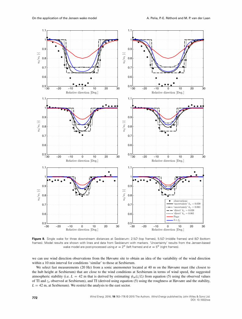
Figure 9 shows an example of such variability within a 10 min interval where the normal distribution is a least squaresfit of the histogram of observed relative directions resulting in � D 3.5ı (this is the typical value found from the analysisperformed for about eighty 10 min histograms of wind direction recorded by the sonic anemometer). As expected, theobserved variability is larger than the value that correlated better with the wake observations at Sexbierum (� D 2ı)because the observed variability should be close to that obtained when adding the effect of the wake expansion and thesimulated additional uncertainty in wind direction.

Table I summarizes the results of comparing quantitatively the Sexbierum data with the models in terms of the windspeed ratio. For the three single wake cases, the Jensen-based wake model using � D 2ı and kw D 0.038 shows the lowestroot mean square error, whereas Fuga’s model the highest.

5.2. Double wake

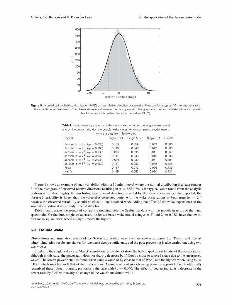
Observations and simulation results of the Sexbierum double wake case are shown in Figure 10. ‘Direct’ and ‘uncer-tainty’ simulation results are shown for two wake decay coefficients, and the post-processing is also carried out using twovalues of � .

Similar to the single wake case, ‘direct’ simulation results do not show the bell-shaped characteristic of the observations,although in this case, the power ratio does not sharply decrease but follows a close to tapered shape due to the superposedwakes. The lowest power deficit is found when using a value of kw close to that of WAsP and the highest when using kw D

0.038, which matches well that of the observations. Again, results of models using Jensen’s approach have traditionallyresembled these ‘direct’ outputs, particularly the case with kw D 0.060. The effect of decreasing kw is a decrease in thepower ratio by 39% with nearly no change in the wake’s maximum width.


773


−30 −20 −10 0 10 20 300.2

0.3

0.4

0.5

0.6

0.7

0.8

0.9

1

1.1

−30 −20 −10 0 10 20 300.2

0.3

0.4

0.5

0.6

0.7

0.8

0.9

1

1.1

−20 0 20

0.5

1


P36/P

38[-]

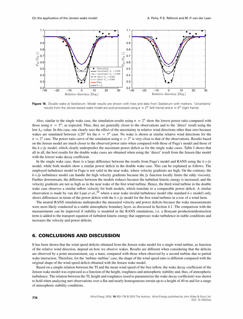
Figure 10. Double wake at Sexbierum. Model results are shown with lines and data from Sexbierum with markers. ‘Uncertainty’results from the Jensen-based wake model are post-processed using � D 2ı (left frame) and � D 5ı (right frame).

Also, similar to the single wake case, the simulation results using � D 2ı show the lowest power ratio compared withthose using � D 5ı, as expected. Thus, they are generally closer to the observations and to the ‘direct’ result using thelow kw-value. In this case, one clearly sees the effect of the uncertainty in relative wind directions other than zero becausewakes are simulated between ˙20ı for the � D 5ı case. No wake is shown at similar relative wind directions for the� D 2ı case. The power ratio curve of the simulation using � D 2ı is very close to that of the observations. Results basedon the Jensen model are much closer to the observed power ratio when compared with those of Fuga’s model and those ofthe k-"-fP model, which clearly underpredict the maximum power deficit as for the single wake cases. Table I shows thatall in all, the best results for the double wake cases are obtained when using the ‘direct’ result from the Jensen-like modelwith the lowest wake decay coefficient.

In the single wake case, there is a large difference between the results from Fuga’s model and RANS using the k-"-fPmodel, while both models show a similar power deficit in the double wake case. This can be explained as follows. Theemployed turbulence model in Fuga is not valid in the near wake, where velocity gradients are high. On the contrary, thek-"-fP turbulence model can handle the high velocity gradients because the fP function locally limits the eddy viscosity.Further downstream, the difference between the models reduces because the turbulent kinetic energy is increased, and thevelocity gradients are not as high as in the near wake of the first wind turbine. Hence, the third wind turbine in the doublewake case observes a similar inflow velocity for both models, which translate to a comparable power deficit. A similarobservation is made by van der Laan et al.,29 where a near wake invalid turbulence model (the standard k-" model) onlyshows differences in terms of the power deficit with the k-"-fP model for the first wind turbines in a row of a wind farm.

The neutral RANS simulations underpredict the measured velocity and power deficits because the wake measurementswere most likely conducted in a stable atmospheric boundary layer, as discussed in Section 4.1. The comparison with themeasurements can be improved if stability is modeled in the RANS simulations, i.e. a Bouyant production/destructionterm is added to the transport equation of turbulent kinetic energy that suppresses wake turbulence in stable conditions andincreases the velocity and power deficits.

6. CONCLUSIONS AND DISCUSSION

It has been shown that the wind speed deficits obtained from the Jensen wake model for a single wind turbine, as functionof the relative wind direction, depend on how we observe wakes. Results are different when considering that the deficitsare observed by a point measurement, say a mast, compared with those when observed by a second turbine due to partialwake interaction. Therefore, for the ‘turbine–turbine’ case, the shape of the wind speed ratio is different compared with theoriginal shape of the wind speed deficit obtained with the Jensen wake model.

Based on a simple relation between the TI and the mean wind speed of the free inflow, the wake decay coefficient of theJensen wake model was expressed as a function of the height, roughness and atmospheric stability and, thus, of atmosphericturbulence. The relation between the TI, height and roughness (used to parameterize the wake decay coefficient) was shownto hold when analyzing met observations over a flat and nearly homogeneous terrain up to a height of 40 m and for a rangeof atmospheric stability conditions.



Although the ‘direct’ wind speed (or power) deficit from the Jensen wake model is constant across the width of thewake, it was shown that the wake deficits can become Gaussian with the maximum wind speed deficits lower and wakeswider than those from the ‘direct’ Jensen-like wake results. This is achieved through averaging of the simulation’s outputin a similar fashion to that in which the wake cases are observed, while partly accounting for the uncertainty in the winddirection using a Gaussian distribution that resembles the observed variability in the wind direction. For a typical wind farm,we should aim at measuring not only the distribution of the wind direction within the averaging period (which is typically10 min, but as turbines react to wind changes much faster, then perhaps 1 min average will be even more appropriate) butalso the distribution of wind direction changes between the averaging periods and that between turbines. van der Laan etal.29 shows how to account practically for the uncertainty in the wind direction.

Further, we demonstrated the ability of an engineering wind farm wake model based on the Jensen wake model tosimulate the single and double Sexbierum wake cases outperforming (for these particular cases) two more advanced ones:a linearized CFD model, Fuga, and a nonlinear CFD RANS wake model that uses a modified k-" turbulence model. It wasshown that the wake decay coefficient for these simulations should be lower (kw D 0.038) than the value recommendedby WAsP (kw D 0.075) when accounting for atmospheric stability during both campaigns, as the observed TI is too lowcompared with that estimated from surface layer parameters assuming a neutral atmosphere.

The wake decay coefficient is the only adjustable parameter of the Jensen-based wake models (wind direction variabilityand uncertainty, which are also adjustable, can be accounted for as part of the post-processing). We show that this coefficientcan be parameterized within the surface layer over a flat and homogeneous terrain. Although these conditions are rather‘ideal’, results from the model described here using the parameterizations in equations (4) and (6) agree well with theWakeBench benchmark cases at Horns Rev I,32 an offshore farm comprising turbines with a hub height of 70 m. We expectthat it can also be used to accurately predict large turbine wake deficits, particularly under unstable and neutral conditions,as under these regimes, the surface layer can easily extend up to � 100–200 m in middle latitudes. Also, atmosphericstability was accounted for in the kw value in Peña et al.6 for data from the Horns Rev I wind farm. A recent study showing,indirectly, the dependency on TI of kw is that of Nygaard.33 He showed very good agreement between a Jensen-like windfarm wake model and data from a northwest-southeast row with up to 20 turbines within the London array wind farm. Heused a wake decay coefficient of 0.04, filtered data with wind speeds about 9 m s�1 and showed that at this wind speed,the observed TI was about 7%. He showed poorer agreement of the model (the simulated power ratios are not that low asthose of the data) for a southwest-northwest row with up to 12 turbines using kw D 0.04, although he showed that for thatparticular row, the observed TI was lower than 5%. Following our approach, a lower wake decay should be used for thissecond case, which will result in deeper deficits.

Jensen-based wake models are inherently not suited to study the wake characteristics in detail, for which more advancedmodels should be used. Here, we show that simple models can predict wake deficits accurately, now in a more transparentfashion as the wake coefficient can be parameterized. This is very important to address current challenges in wind farmoptimization, as such simple models can be used during the first phase of wind farm layout design due to their efficiency,perhaps followed by a detailed CFD-based analysis. The model here described takes �74 s to estimate the annual energyproduction of an 80 turbine wind farm based on met data collected hourly over 1 year.

ACKNOWLEDGEMENTS

Funding from the EERA DTOC project (contract FP7-ENERGY-2011/n 282797) is acknowledged. This work is carried outas part of the IEA-WakeBench research collaboration project partly funded by EUDP WakeBench (contract 64011-0308).

REFERENCES

1. Jensen NO, A note on wind generator interaction, Technical Report Risoe-M-2411(EN), Risø National Laboratory,Roskilde, 1983.

2. Katic I, Højstrup J, Jensen NO. A simple model for cluster efficiency. Proceedings of the European Wind EnergyAssociation Conference & Exhibition, Rome, 1986; 407–410.

3. Mortensen NG, Heathfield DN, Myllerup L, Landberg L, Rathmann O, Getting started with WAsP 9, Technical ReportRisø-I-2571(EN), Risø National Laboratory, Roskilde, 2007.

4. Nielsen P, Case studies calculating wind farm production, Technical Report, EMD Energi- og Miljødata, Aalborg,2002.

5. Gaumond M, Rethoré PE, Ott S, Peña A, Bechmann A, Hansen KS. Evaluation of the wind direction uncertainty andits impact on wake modelling at the Horns Rev offshore wind farm. Wind Energy 2014; 17: 1169–1178.

6. Peña A, Réthoré P-E, Rathmann O. Modeling large offshore wind farms under different atmospheric stability regimeswith the park wake model. Renewable Energy 2014; 70: 164–171.


775


7. Ott S, Berg J, Nielsen M, Linearised CFD models for wakes, Technical Report Risø–R–1772(EN), Risø NationalLaboratory for Sustainable Energy, Roskilde, 2011.

8. Gaumond M, Evaluation and benchmarking of wind turbine wake models, Technical Report Master Thesis, DTU WindEnergy, Roskilde, 2012.

9. Sørensen NN, General purpose flow solver applied to flow over hills, Technical Report Risø-R-827(EN), Risø NationalLaboratory, Roskilde, 2003.

10. Troldborg N, Actuator line modeling of wind turbine wakes, Technical Report PhD Thesis, Technical University ofDenmark, Lyngby, 2008.

11. Wan C, Wang J, Yang G, Gu H, Zhang X. Wind farm micro-siting by Gaussian particle swarm optimization with localsearch strategy. Renewable Energy 2012; 48: 276–286.

12. Peña A, Rathmann O. Atmospheric stability-dependent infinite wind-farm models and the wake-decay coefficient.Wind Energy 2014; 17: 1269–1285.

13. Frandsen S. On the wind speed reduction in the center of large clusters of wind turbines. Journal of Wind Engineeringand Industrial Aerodynamics 1992; 39: 251–265.

14. Stull RB. An Introduction to Boundary Layer Meteorology. Kluwer Academic Publishers: Dordrecht, 1988.15. Obukhov AM. Turbulence in an atmosphere with a non-uniform temperature. Boundary-Layer Meteorology 1971; 2:

7–29.16. Peña A, Gryning SE. Hasager CB. Measurements and modelling of the wind speed profile in the marine atmospheric

boundary layer. Boundary-Layer Meteorology 2008; 129: 479–495.17. Peña A, Gryning SE. Hasager CB. Comparing mixing-length models of the diabatic wind profile over homogeneous

terrain. Theoretical and Applied Climatology 2010; 100: 325–335.18. Holtslag AAM. Estimates of diabatic wind speed profiles from near-surface weather observations. Boundary-Layer

Meteorology 1984; 29: 225–250.19. Panofsky HA, Dutton JA. Atmospheric Turbulence. John Wiley & Sons: New York, 1984.20. Peña A, Gryning SE. Mann J. On the length-scale of the wind profile. Quarterly Journal of the Royal Meteorological

Society 2010; 136: 2119–2131.21. Peña A, Floors R, Gryning S.-E. The Høvsøre tall wind-profile experiment: a description of wind profile observations

in the atmospheric boundary layer. Boundary-Layer Meteorology 2014; 150: 69–89.22. Peña A, Sensing the wind profile, Technical Report Risø-PhD-45(EN), Risø DTU, Roskilde, 2009.23. Peña A, Gryning SE. Mann J, Hasager CB. Length scales of the neutral wind profile over homogeneous terrain. Journal

of Applied Meteorology and Climatology 2010; 49: 792–806.24. Peña A, Gryning SE, Hahmann AN. Observations of the atmospheric boundary layer height under marine upstream

flow conditions at a coastal site. Journal of Geophysical Research-Atmospheres 2013; 118: 1924–1940.25. Peña A, Floors R, Wagner R, Courtney MS, Gryning SE, Sathe A, Lars?n XG, Hahmann AN, Hasager CB. Ten years

of boundary-layer and wind-power meteorology at Høvsøre, Denmark. Boundary-Layer Meteorology 2015. In review.26. Gryning SE, Batchvarova E, Brümmer B, Jørgensen H, Larsen S. On the extension of the wind profile over

homogeneous terrain beyond the surface layer. Boundary-Layer Meteorology 2007; 124: 251–268.27. van der Laan MP, Sørensen NN, Réthoré PE, Mann J, Kelly MC, Troldborg N, Schepers JG, Machefaux E. An

improved k-" model applied to a wind turbine wake in atmospheric turbulence. Wind Energy 2015; 18: 889–907.28. van der Laan MP, Sørensen NN, Réthoré PE, Mann J, Kelly MC, Troldborg N. The k-"-fp model applied to double

wind turbine wakes using different actuator disk force methods. Wind Energy 2014. DOI: 10.1002/we.1816.29. van der Laan MP, Sørensen NN, Réthoré PE, Mann J, Kelly MC, Troldborg N, Hansen KS, Murcia JP. The k-"-fp

model applied to wind farms. Wind Energy 2014. DOI: 10.1002/we.1804.30. Cleijne JW, Results of the Sexbierum wind farm; double wake measurements, Technical Report 92-388, TNO

Environmental and Energy Research, Apeldoorn, Netherlands, 1992.31. Cleijne JW, Results of the Sexbierum wind farm; single wake measurements, Technical Report 93-082, TNO

Environmental and Energy Research, Apeldoorn, Netherlands, 1993.32. Peña A, Réthoré PE, Hasager CB, Hansen K, Results of wake simulations at the Horns Rev I and Lillgrund wind

farms using the modified Park model, Technical Report DTU Wind Energy-E-Report-0026(EN), DTU Wind Energy,Roskilde, 2013.

33. Nygaard NG. Wakes in very large wind farms and the effect of neighbouring wind farms. Journal of Physics ConferenceSeries 2014; 524: 012162 (10 pp).


Documents

On the application of the Jensen wake model using a ...orbit.dtu.dk/files/122284235/On_the_application_of_the_Jensen_wake... · Pena Diaz, A., Réthoré, P-E., & van der Laan, P