Multiple TestingMultiple Testing

Mark J. van der LaanMark J. van der LaanDivision of BiostatisticsDivision of Biostatistics

U.C. BerkeleyU.C. Berkeley

www.stat.berkeley.edu/~laanwww.stat.berkeley.edu/~laan

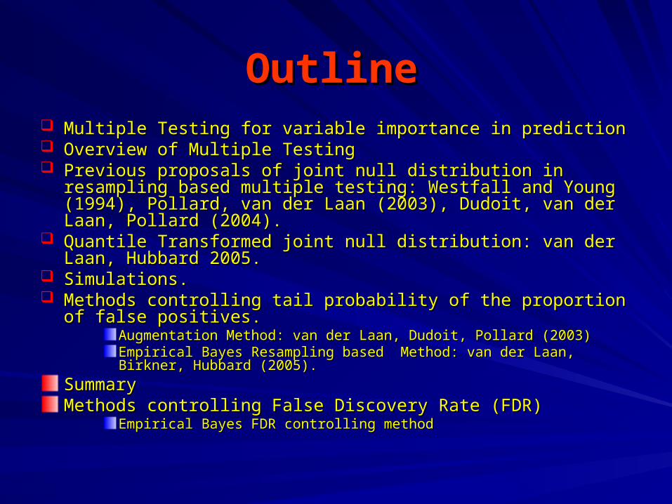
OutlineOutline Multiple Testing for variable importance in predictionMultiple Testing for variable importance in prediction Overview of Multiple TestingOverview of Multiple Testing Previous proposals of joint null distribution in resampling based Previous proposals of joint null distribution in resampling based

multiple testing: Westfall and Young (1994), Pollard, van der Laan multiple testing: Westfall and Young (1994), Pollard, van der Laan (2003), Dudoit, van der Laan, Pollard (2004).(2003), Dudoit, van der Laan, Pollard (2004).

Quantile Transformed joint null distribution: van der Laan, Hubbard Quantile Transformed joint null distribution: van der Laan, Hubbard 2005.2005.

Simulations.Simulations. Methods controlling tail probability of the proportion of false Methods controlling tail probability of the proportion of false

positives.positives.Augmentation Method: van der Laan, Dudoit, Pollard (2003)Augmentation Method: van der Laan, Dudoit, Pollard (2003)Empirical Bayes Resampling based Method: van der Laan, Birkner, Empirical Bayes Resampling based Method: van der Laan, Birkner, Hubbard (2005).Hubbard (2005).

SummarySummaryMethods controlling False Discovery Rate (FDR)Methods controlling False Discovery Rate (FDR)

Empirical Bayes FDR controlling methodEmpirical Bayes FDR controlling method

Multiple Testing in PredictionMultiple Testing in Prediction

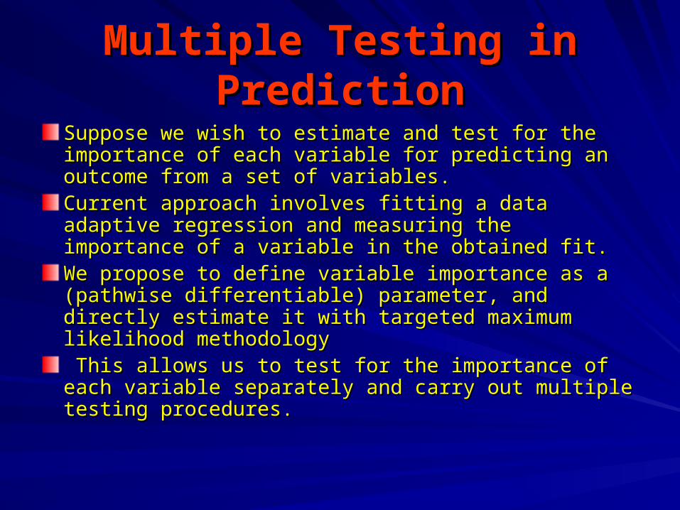
Suppose we wish to estimate and test for the importance Suppose we wish to estimate and test for the importance of each variable for predicting an outcome from a set of of each variable for predicting an outcome from a set of variables.variables.Current approach involves fitting a data adaptive Current approach involves fitting a data adaptive regression and measuring the importance of a variable in regression and measuring the importance of a variable in the obtained fit.the obtained fit.We propose to define variable importance as a (pathwise We propose to define variable importance as a (pathwise differentiable) parameter, and directly estimate it with differentiable) parameter, and directly estimate it with targeted maximum likelihood methodologytargeted maximum likelihood methodology This allows us to test for the importance of each variable This allows us to test for the importance of each variable separately and carry out multiple testing procedures.separately and carry out multiple testing procedures.

Example: HIV resistance Example: HIV resistance mutationsmutations

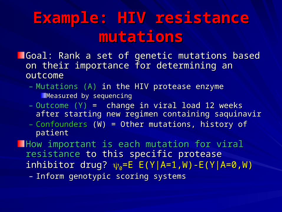
Goal: Rank a set of genetic mutations based on Goal: Rank a set of genetic mutations based on their importance for determining an outcometheir importance for determining an outcome– MutationsMutations (A)(A) in the HIV protease enzyme in the HIV protease enzyme

Measured by sequencingMeasured by sequencing

– Outcome (Y)Outcome (Y) = change in viral load 12 weeks after = change in viral load 12 weeks after starting new regimen containing saquinavirstarting new regimen containing saquinavir

– ConfoundersConfounders (W) = Other mutations, history of patient (W) = Other mutations, history of patient

How important is each mutation for viral How important is each mutation for viral resistanceresistance to this specific protease inhibitor to this specific protease inhibitor drug? drug? 00=E E(Y|A=1,W)-E(Y|A=0,W)=E E(Y|A=1,W)-E(Y|A=0,W)– Inform genotypic scoring systemsInform genotypic scoring systems

Targeted Maximum LikelihoodTargeted Maximum Likelihood

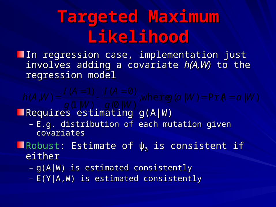
In regression case, implementation just involves In regression case, implementation just involves adding a covariate adding a covariate h(A,W)h(A,W) to the regression to the regression modelmodel

Requires estimating g(A|W)Requires estimating g(A|W)– E.g. distribution of each mutation given covariatesE.g. distribution of each mutation given covariates

RobustRobust: Estimate of : Estimate of ψψ00 is consistent if either is consistent if either– g(A|W) is estimated consistentlyg(A|W) is estimated consistently– E(Y|A,W) is estimated consistentlyE(Y|A,W) is estimated consistently

)|Pr()|( where,)|0(

)0(

)|1(

)1(),( WaAWag

Wg

AI

Wg

AIWAh

Mutation Rankings Based on Mutation Rankings Based on Variable ImportanceVariable Importance

Current ScoreCurrent Score MutationMutation VIMVIM VIM p-valueVIM p-value CrudeCrude Crude p-valueCrude p-value

3535 90M90M 0.700.70 0.000.00 0.760.76 0.000.00

4040 48VM48VM 0.790.79 0.000.00 1.071.07 0.000.00

00 30N30N -0.78-0.78 0.000.00 -1.06-1.06 0.000.00

1010 82AFST82AFST 0.460.46 0.010.01 0.350.35 0.030.03

1010 54VA54VA 0.460.46 0.010.01 0.310.31 0.110.11

1010 73CSTA73CSTA 0.670.67 0.030.03 0.800.80 0.000.00

22 20IMRTVL20IMRTVL 0.320.32 0.070.07 0.260.26 0.180.18

11 36ILVTA36ILVTA 0.280.28 0.100.10 0.270.27 0.120.12

22 10FIRVY10FIRVY 0.270.27 0.130.13 0.480.48 0.000.00

55 88DTG88DTG -0.23-0.23 0.240.24 -0.50-0.50 0.330.33

22 71TVI71TVI 0.180.18 0.290.29 0.140.14 0.370.37

55 32I32I -0.18-0.18 0.580.58 -0.20-0.20 0.550.55

22 63P63P 0.060.06 0.770.77 0.110.11 0.560.56

55 46ILV46ILV 0.130.13 0.980.98 0.270.27 0.100.10

Hypothesis Testing IngredientsHypothesis Testing Ingredients

Data (XData (X11,…,X,…,Xnn))

HypothesesHypotheses

Test StatisticsTest Statistics

Type I ErrorType I Error

Null DistributionNull DistributionMarginal (p-values) or Marginal (p-values) or

Joint distribution of the test statisticsJoint distribution of the test statistics

Rejection RegionRejection Region

Adjusted p-valuesAdjusted p-values

Test StatisticsTest Statistics

A test statistic is written as:A test statistic is written as:

TTnn= = ((nn - - 00))

n n

Where Where nn is the standard error, is the standard error, nn is the is the

parameter of interest, and parameter of interest, and 00 is the null is the null

value of the parameter.value of the parameter.

HypothesesHypotheses

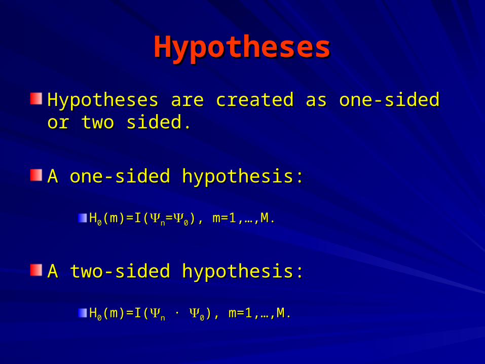
Hypotheses are created as one-sided or two Hypotheses are created as one-sided or two sided.sided.

A one-sided hypothesis:A one-sided hypothesis:

HH00(m)=I((m)=I(nn==00), m=1,…,M.), m=1,…,M.

A two-sided hypothesis:A two-sided hypothesis:

HH00(m)=I((m)=I(nn ·· 00), m=1,…,M.), m=1,…,M.

Type I & II ErrorsType I & II Errors

Type I errorsType I errors corresponds to making a false corresponds to making a false positive.positive.

Type II errors (Type II errors ()) corresponds to making a false corresponds to making a false negative.negative.

TheThe Power Power is defined as 1- is defined as 1-

Multiple Testing Procedures are interested in Multiple Testing Procedures are interested in simultaneously minimizing the Type I error rate simultaneously minimizing the Type I error rate while maximizing power.while maximizing power.

Type I Error RatesType I Error Rates

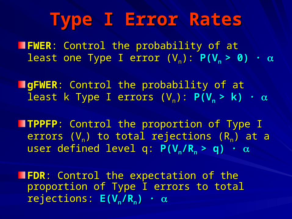
FWERFWER: Control the probability of at least one : Control the probability of at least one Type I error (VType I error (Vnn): ): P(VP(Vn n > 0) > 0) ··

gFWERgFWER: Control the probability of at least k : Control the probability of at least k Type I errors (VType I errors (Vnn): ): P(VP(Vn n > k) > k) ··

TPPFPTPPFP: Control the proportion of Type I errors : Control the proportion of Type I errors (V(Vnn) to total rejections (R) to total rejections (Rnn) at a user defined level ) at a user defined level q: q: P(VP(Vnn/R/Rn n > q) > q) ··

FDRFDR: Control the expectation of the proportion of : Control the expectation of the proportion of Type I errors to total rejections: Type I errors to total rejections: E(VE(Vnn/R/Rnn) ) ··

Null DistributionNull Distribution

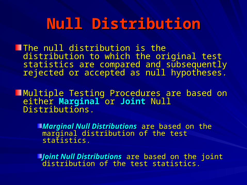
The null distribution is the distribution to which The null distribution is the distribution to which the original test statistics are compared and the original test statistics are compared and subsequently rejected or accepted as null subsequently rejected or accepted as null hypotheses.hypotheses.

Multiple Testing Procedures are based on either Multiple Testing Procedures are based on either MarginalMarginal or or JointJoint Null Distributions. Null Distributions.

Marginal Null DistributionsMarginal Null Distributions are based on the are based on the marginal distribution of the test statistics.marginal distribution of the test statistics.

Joint Null DistributionsJoint Null Distributions are based on the joint are based on the joint distribution of the test statistics.distribution of the test statistics.

Rejection RegionsRejection Regions

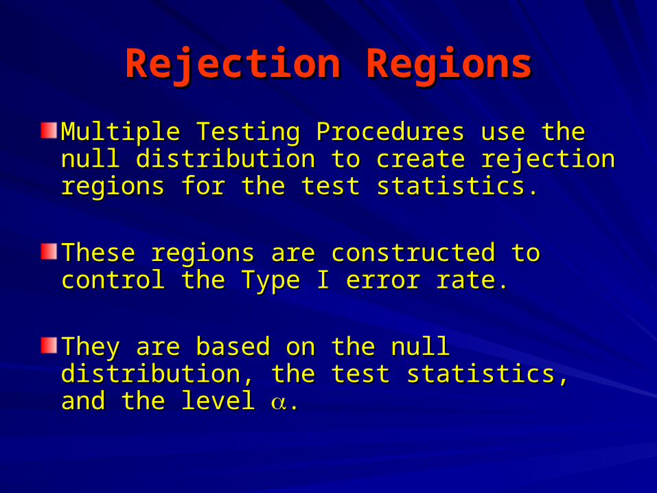
Multiple Testing Procedures use the null Multiple Testing Procedures use the null distribution to create rejection regions for distribution to create rejection regions for the test statistics. the test statistics.

These regions are constructed to control These regions are constructed to control the Type I error rate.the Type I error rate.

They are based on the null distribution, the They are based on the null distribution, the test statistics, and the level test statistics, and the level . .

Single-Step & StepwiseSingle-Step & Stepwise

Single-stepSingle-step procedures assess each null procedures assess each null hypothesis using a rejection region which hypothesis using a rejection region which is independent of the tests of other is independent of the tests of other hypotheses.hypotheses.

StepwiseStepwise procedures construct rejection procedures construct rejection regions based on the acceptance/rejection regions based on the acceptance/rejection of other hypotheses. They are applied to of other hypotheses. They are applied to smaller nested subsets of tests (e.g. Step-smaller nested subsets of tests (e.g. Step-down procedures).down procedures).

Adjusted p-valuesAdjusted p-values

Adjusted p-values are constructed as Adjusted p-values are constructed as summary measures for the test statistics.summary measures for the test statistics.

We can think of the adjusted p-value We can think of the adjusted p-value p(m)p(m) as the nominal level as the nominal level at which test at which test statistic statistic T(m)T(m) would have just been would have just been rejected. rejected.

Multiple Testing ProceduresMultiple Testing Procedures

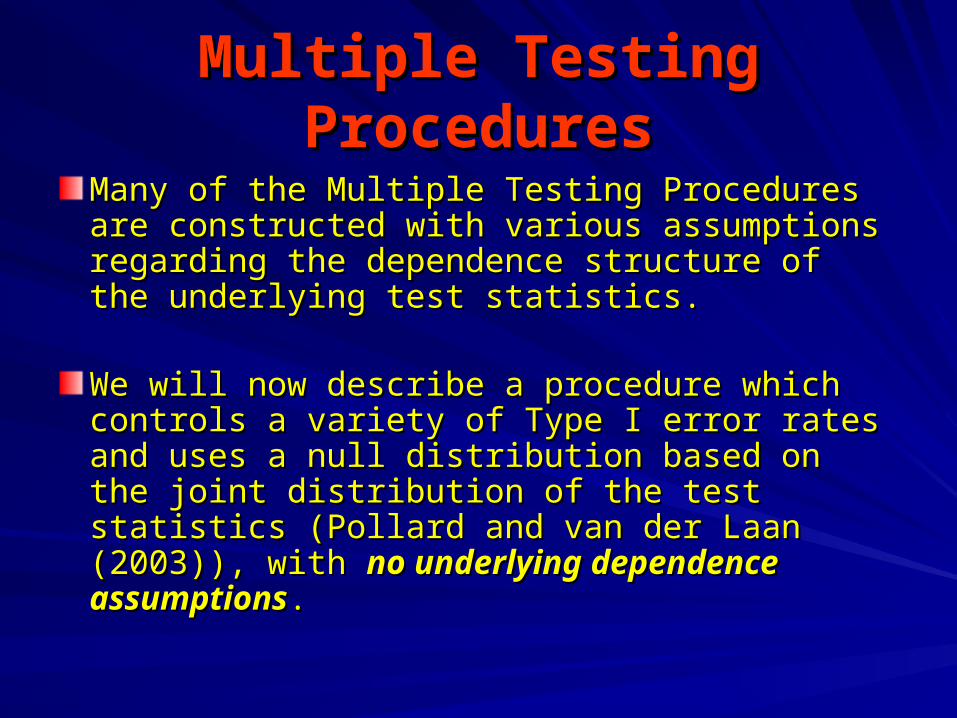
Many of the Multiple Testing Procedures are Many of the Multiple Testing Procedures are constructed with various assumptions regarding constructed with various assumptions regarding the dependence structure of the underlying test the dependence structure of the underlying test statistics. statistics.

We will now describe a procedure which controls We will now describe a procedure which controls a variety of Type I error rates and uses a null a variety of Type I error rates and uses a null distribution based on the joint distribution of the distribution based on the joint distribution of the test statistics (Pollard and van der Laan (2003)), test statistics (Pollard and van der Laan (2003)), with with no underlying dependence assumptionsno underlying dependence assumptions..

Null Distribution Null Distribution (Pollard & van der Laan (2003))(Pollard & van der Laan (2003))

This approach is interested in Type I error control under the true data This approach is interested in Type I error control under the true data generating distribution, as opposed to the data generating null generating distribution, as opposed to the data generating null distribution, which does not always provide control under the true distribution, which does not always provide control under the true underlying distribution (e.g. Westfall & Young).underlying distribution (e.g. Westfall & Young).

We want to use the null distribution to derive rejection regions for the We want to use the null distribution to derive rejection regions for the test statistics such that the Type I error rate is (asymptotically) test statistics such that the Type I error rate is (asymptotically) controlled at desired level controlled at desired level . .

In practice, the true distribution In practice, the true distribution QQnn=Q=Qnn(P)(P), for the test statistics T, for the test statistics Tnn, is , is unknown and replaced by a null distribution unknown and replaced by a null distribution QQ00 (or estimate, (or estimate, QQ0n0n). ).

The proposed null distribution QThe proposed null distribution Q00 is the asymptotic distribution of the is the asymptotic distribution of the vector of null value shifted and scaled test statistics, which provides vector of null value shifted and scaled test statistics, which provides the desired asymptotic control of the Type I error rate. the desired asymptotic control of the Type I error rate.

t-statistics:t-statistics: For the test of single-parameter null hypotheses using t- For the test of single-parameter null hypotheses using t-statistics the null distribution Qstatistics the null distribution Q00 is an M--variate Gaussian is an M--variate Gaussian distribution. distribution.

QQ00 = Q = Q00(P) (P) ´́ N(0, N(0,**(P)).(P)).

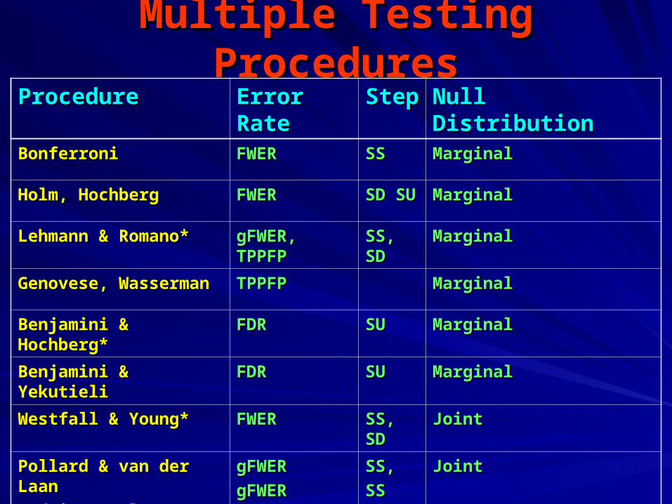
Multiple Testing ProceduresMultiple Testing ProceduresProcedureProcedure Error RateError Rate StepStep Null DistributionNull Distribution

BonferroniBonferroni FWERFWER SSSS MarginalMarginal

Holm, HochbergHolm, Hochberg FWERFWER SD SUSD SU MarginalMarginal

Lehmann & Romano*Lehmann & Romano* gFWER, gFWER, TPPFPTPPFP

SS, SS, SDSD

MarginalMarginal

Genovese, WassermanGenovese, Wasserman TPPFPTPPFP MarginalMarginal

Benjamini & Hochberg*Benjamini & Hochberg* FDRFDR SUSU MarginalMarginal

Benjamini & YekutieliBenjamini & Yekutieli FDRFDR SUSU MarginalMarginal

Westfall & Young*Westfall & Young* FWERFWER SS, SS, SDSD

JointJoint

Pollard & van der LaanPollard & van der Laan

Dudoit et al.Dudoit et al.

van der Laan et al. ‘svan der Laan et al. ‘s

gFWER gFWER

gFWERgFWER

FWE, TPPFPFWE, TPPFP

SS, SS,

SSSS

SDSD

JointJoint

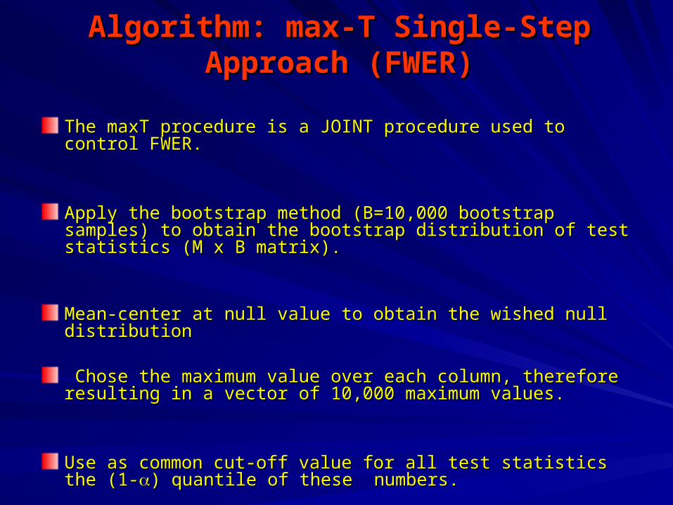
Algorithm: max-T Single-Step Approach Algorithm: max-T Single-Step Approach (FWER)(FWER)

The maxT procedure is a JOINT procedure used to control FWER. The maxT procedure is a JOINT procedure used to control FWER.

Apply the bootstrap method (B=10,000 bootstrap samples) to obtain Apply the bootstrap method (B=10,000 bootstrap samples) to obtain the bootstrap distribution of test statistics (M x B matrix). the bootstrap distribution of test statistics (M x B matrix).

Mean-center at null value to obtain the wished null distributionMean-center at null value to obtain the wished null distribution

Chose the maximum value over each column, therefore resulting in Chose the maximum value over each column, therefore resulting in a vector of 10,000 maximum values.a vector of 10,000 maximum values.

Use as common cut-off value for all test statistics the (1-Use as common cut-off value for all test statistics the (1-) quantile ) quantile of these numbers.of these numbers.

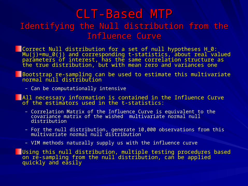
CLT-Based MTPCLT-Based MTPIdentifying the Null distribution from the Influence CurveIdentifying the Null distribution from the Influence Curve

Correct Null distribution for a set of null hypotheses H_0: Mu(j)=mu_0(j) Correct Null distribution for a set of null hypotheses H_0: Mu(j)=mu_0(j) and corresponding t-statistics, about real valued parameters of interest, and corresponding t-statistics, about real valued parameters of interest, has the same correlation structure as the true distribution, but with mean has the same correlation structure as the true distribution, but with mean zero and variances onezero and variances one

Bootstrap re-sampling can be used to estimate this multivariate normal null Bootstrap re-sampling can be used to estimate this multivariate normal null distributiondistribution

– Can be computationally intensiveCan be computationally intensive

All necessary information is contained in the Influence Curve of the All necessary information is contained in the Influence Curve of the estimators used in the t-statistics:estimators used in the t-statistics:

– Correlation Matrix of the Influence Curve is equivalent to the covariance matrix Correlation Matrix of the Influence Curve is equivalent to the covariance matrix of the wished multivariate normal null distributionof the wished multivariate normal null distribution

– For the null distribution, generate 10,000 observations from this multivariate For the null distribution, generate 10,000 observations from this multivariate normal null distributionnormal null distribution

– VIM methods naturally supply us with the influence curveVIM methods naturally supply us with the influence curve

Using this null distribution, multiple testing procedures based on re-Using this null distribution, multiple testing procedures based on re-sampling from the null distribution, can be applied quickly and easilysampling from the null distribution, can be applied quickly and easily

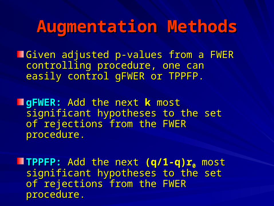
Augmentation MethodsAugmentation Methods

Given adjusted p-values from a FWER Given adjusted p-values from a FWER controlling procedure, one can easily control controlling procedure, one can easily control gFWER or TPPFP.gFWER or TPPFP.

gFWER:gFWER: Add the next Add the next kk most significant most significant hypotheses to the set of rejections from the hypotheses to the set of rejections from the FWER procedure.FWER procedure.

TPPFP:TPPFP: Add the next Add the next (q/1-q)r(q/1-q)r00 most most significant hypotheses to the set of rejections significant hypotheses to the set of rejections from the FWER procedure. from the FWER procedure.

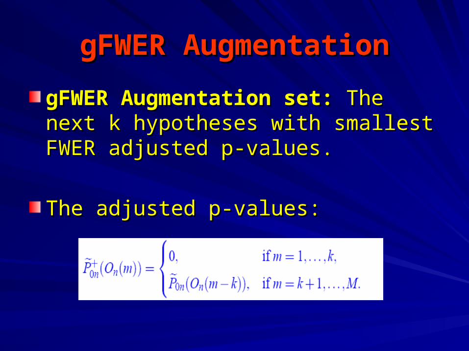
gFWER AugmentationgFWER Augmentation

gFWER Augmentation set:gFWER Augmentation set: The next k The next k hypotheses with smallest FWER adjusted hypotheses with smallest FWER adjusted p-values.p-values.

The adjusted p-values:The adjusted p-values:

TPPFP AugmentationTPPFP AugmentationTPPFP Augmentation set:TPPFP Augmentation set: The next hypotheses The next hypotheses with the smallest FWER adjusted p-values where with the smallest FWER adjusted p-values where one keeps rejecting null hypotheses until the ratio of one keeps rejecting null hypotheses until the ratio of additional rejections to the total number of rejections additional rejections to the total number of rejections reaches the allowed proportion q of false positives.reaches the allowed proportion q of false positives.

The adjusted p-values:The adjusted p-values:

TPPFP TechniqueTPPFP TechniqueThe TPPFP Technique was created as a less conservative and The TPPFP Technique was created as a less conservative and more powerful method of controlling the tail probability of the more powerful method of controlling the tail probability of the proportion of false positives.proportion of false positives.

This technique is based on constructing a distribution of the set of This technique is based on constructing a distribution of the set of null hypotheses null hypotheses SS0n0n, as well as a distribution under the null , as well as a distribution under the null hypothesis (hypothesis (TTnn). We are interested in controlling the random ). We are interested in controlling the random variable variable rrnn(c)(c)..

The distribution under the null is the identical null distribution used in The distribution under the null is the identical null distribution used in Pollard and van der Laan (2003): mean centered joint distribution of Pollard and van der Laan (2003): mean centered joint distribution of test-statistics.test-statistics.

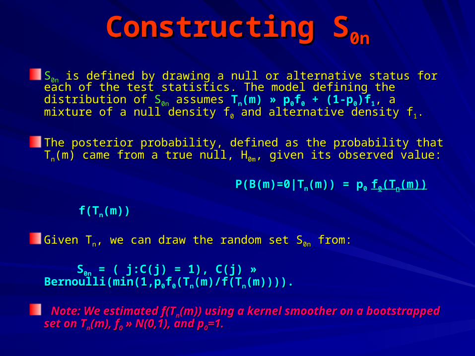
Constructing SConstructing S0n0n

SS0n0n is defined by drawing a null or alternative status for each of the is defined by drawing a null or alternative status for each of the test statistics. The model defining the distribution of test statistics. The model defining the distribution of SS0n0n assumes assumes TTnn(m) (m) »» p p00ff00 + (1-p + (1-p00)f)f11, a mixture of a null density f, a mixture of a null density f00 and alternative and alternative density fdensity f11..

The posterior probability, defined as the probability that TThe posterior probability, defined as the probability that Tnn(m) came (m) came from a true null, Hfrom a true null, H0m0m, given its observed value: , given its observed value:

P(B(m)=0|TP(B(m)=0|Tnn(m)) = p(m)) = p0 0 ff00(T(Tnn(m))(m)) f(Tf(Tnn(m))(m))

Given TGiven Tnn, we can draw the random set S, we can draw the random set S0n0n from: from: SS0n0n = ( j:C(j) = 1), C(j) = ( j:C(j) = 1), C(j) »» Bernoulli(min(1,p Bernoulli(min(1,p00ff00(T(Tnn(m)/f(T(m)/f(Tnn(m)))).(m)))).

Note: We estimated f(TNote: We estimated f(Tnn(m)) using a kernel smoother on a (m)) using a kernel smoother on a bootstrapped set on Tbootstrapped set on Tnn(m), f(m), f00 »» N(0,1), and p N(0,1), and p00=1.=1.

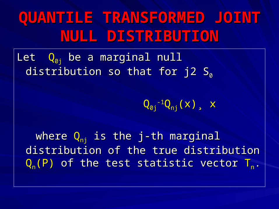
QUANTILE TRANSFORMED QUANTILE TRANSFORMED JOINT NULL DISTRIBUTIONJOINT NULL DISTRIBUTION

Let Let QQ0j0j be a marginal null distribution so that be a marginal null distribution so that

for jfor j22 S S00

QQ0j0j-1-1QQnjnj(x)(x)¸̧ x x

where where QQnjnj is the j-th marginal distribution of is the j-th marginal distribution of

the true distribution the true distribution QQnn(P)(P) of the test statistic of the test statistic

vector vector TTnn..

QUANTILE TRANSFORMED QUANTILE TRANSFORMED JOINT NULL DISTRUTIONJOINT NULL DISTRUTION

We propose as null distribution the We propose as null distribution the distribution distribution QQ0n0n of of

TTnn**(j)=Q(j)=Q0j0j

-1-1QQnjnj(T(Tnn(j)), j=1,…,J(j)), j=1,…,J

This joint null distribution This joint null distribution QQ0n0n(P)(P) does indeed does indeed

satisfy the wished multivariate asymptotic satisfy the wished multivariate asymptotic domination condition in (Dudoit, van der domination condition in (Dudoit, van der Laan, Pollard, 2004).Laan, Pollard, 2004).

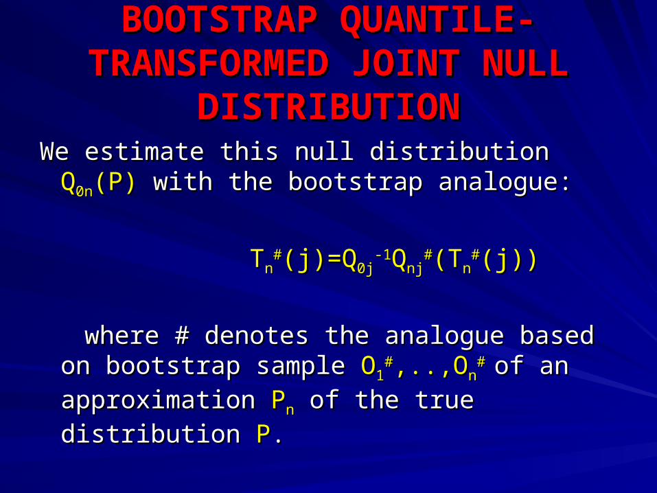
We estimate this null distribution We estimate this null distribution QQ0n0n(P)(P) with with

the bootstrap analogue:the bootstrap analogue:

TTnn##(j)=Q(j)=Q0j0j

-1-1QQnjnj##(T(Tnn

##(j))(j))

where # denotes the analogue based on where # denotes the analogue based on bootstrap sample bootstrap sample OO11

##,..,O,..,Onn## of an of an

approximation approximation PPnn of the true distribution of the true distribution PP. .

BOOTSTRAP QUANTILE-BOOTSTRAP QUANTILE-TRANSFORMED JOINT NULL TRANSFORMED JOINT NULL

DISTRIBUTIONDISTRIBUTION

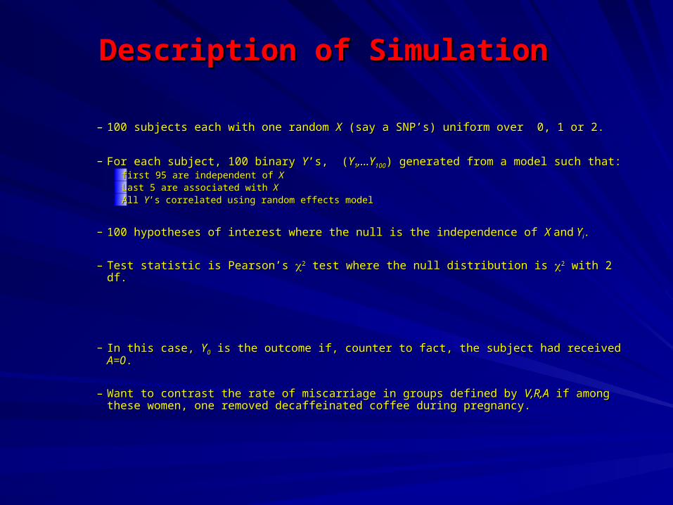
Description of SimulationDescription of Simulation

– 100 subjects each with one random 100 subjects each with one random XX (say a SNP’s) uniform over 0, 1 or 2. (say a SNP’s) uniform over 0, 1 or 2.

– For each subject, 100 binary For each subject, 100 binary YY’s, (’s, (YY11,...Y,...Y100100) generated from a model such that:) generated from a model such that:first 95 are independent of first 95 are independent of XXLast 5 are associated with Last 5 are associated with XXAll All YY’s correlated using random effects model’s correlated using random effects model

– 100 hypotheses of interest where the null is the independence of 100 hypotheses of interest where the null is the independence of X X andand Y Yi i ..

– Test statistic is Pearson’s Test statistic is Pearson’s 22 test where the null distribution is test where the null distribution is 22 with 2 df. with 2 df.

– In this case, In this case, YY00 is the outcome if, counter to fact, the subject had received is the outcome if, counter to fact, the subject had received A=0A=0..

– Want to contrast the rate of miscarriage in groups defined by Want to contrast the rate of miscarriage in groups defined by V,R,AV,R,A if among these women, if among these women, one removed decaffeinated coffee during pregnancy.one removed decaffeinated coffee during pregnancy.

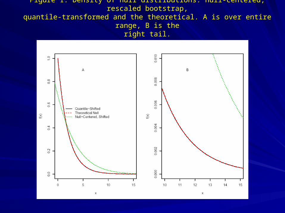
Figure 1: Density of null distributions: null-centered, rescaled bootstrap,Figure 1: Density of null distributions: null-centered, rescaled bootstrap,quantile-transformed and the theoretical. A is over entire range, B is thequantile-transformed and the theoretical. A is over entire range, B is the

right tail.right tail.

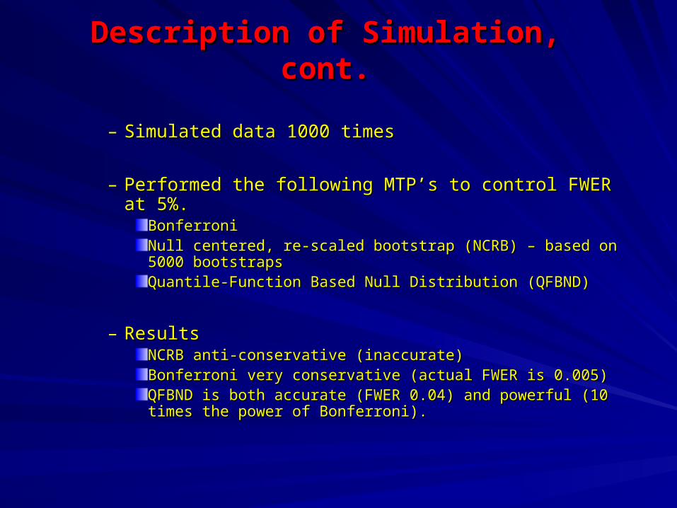
Description of Simulation, cont.Description of Simulation, cont.

– Simulated data 1000 timesSimulated data 1000 times

– Performed the following MTP’s to control FWER at 5%.Performed the following MTP’s to control FWER at 5%.BonferroniBonferroniNull centered, re-scaled bootstrap (NCRB) – based on 5000 bootstrapsNull centered, re-scaled bootstrap (NCRB) – based on 5000 bootstrapsQuantile-Function Based Null Distribution (QFBND)Quantile-Function Based Null Distribution (QFBND)

– ResultsResultsNCRB anti-conservative (inaccurate)NCRB anti-conservative (inaccurate)Bonferroni very conservative (actual FWER is 0.005)Bonferroni very conservative (actual FWER is 0.005)QFBND is both accurate (FWER 0.04) and powerful (10 times the QFBND is both accurate (FWER 0.04) and powerful (10 times the power of Bonferroni).power of Bonferroni).

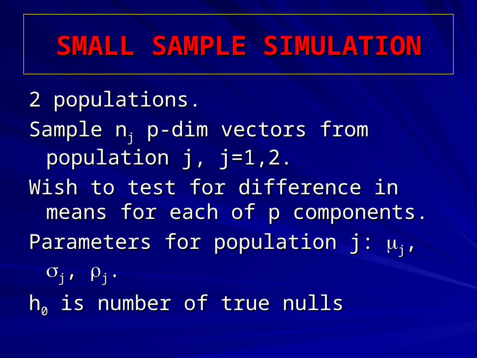
SMALL SAMPLE SIMULATIONSMALL SAMPLE SIMULATION

2 populations. 2 populations.

Sample nSample njj p-dim vectors from population j, p-dim vectors from population j,

j=1,2.j=1,2.

Wish to test for difference in means for each Wish to test for difference in means for each of p components.of p components.

Parameters for population j: Parameters for population j: jj, , jj, , jj..

hh00 is number of true nulls is number of true nulls

COMBINING PERMUTATION COMBINING PERMUTATION DISTRIBUTION WITH QUANTILE DISTRIBUTION WITH QUANTILE

NULL DISTRIBUTIONNULL DISTRIBUTIONFor a test of independence, the For a test of independence, the permutation distribution is the preferred permutation distribution is the preferred choice of marginal null distribution, due to choice of marginal null distribution, due to its finite sample control.its finite sample control.We can construct a quantile transformed We can construct a quantile transformed joint null distribution whose marginals joint null distribution whose marginals equal these permutation distributions, and equal these permutation distributions, and use this distribution to control any wished use this distribution to control any wished type I error rate. type I error rate.

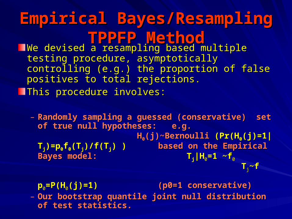
Empirical Bayes/Resampling Empirical Bayes/Resampling TPPFP MethodTPPFP Method

We devised a resampling based multiple testing We devised a resampling based multiple testing procedure, asymptotically controlling (e.g.) the procedure, asymptotically controlling (e.g.) the proportion of false positives to total rejections. proportion of false positives to total rejections. This procedure involves:This procedure involves:

– Randomly sampling a guessed (conservative) set Randomly sampling a guessed (conservative) set of true null hypotheses: e.g. of true null hypotheses: e.g. HH00(j)~Bernoulli (j)~Bernoulli (Pr(H(Pr(H00(j)=1|T(j)=1|Tjj)=p)=p00ff00(T(Tjj)/f(T)/f(Tjj) )) ) based based on the Empirical Bayes model: on the Empirical Bayes model: TTjj|H|H00=1 ~f=1 ~f0 0 TTjj~f ~f pp00=P(H=P(H00(j)=1)(j)=1) (p0=1 conservative) (p0=1 conservative)

– Our bootstrap quantile joint null distribution of test Our bootstrap quantile joint null distribution of test statistics.statistics.

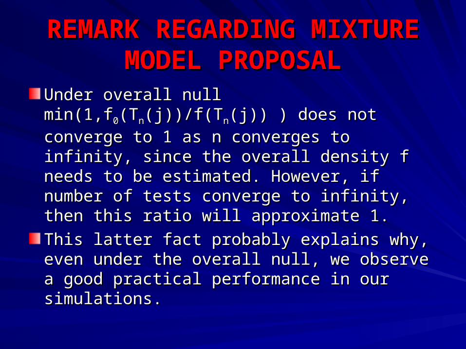
REMARK REGARDING MIXTURE REMARK REGARDING MIXTURE MODEL PROPOSALMODEL PROPOSAL

Under overall null min(1,fUnder overall null min(1,f00(T(Tnn(j))/f(T(j))/f(Tnn(j)) ) does (j)) ) does

not converge to 1 as n converges to infinity, not converge to 1 as n converges to infinity, since the overall density f needs to be estimated. since the overall density f needs to be estimated. However, if number of tests converge to infinity, However, if number of tests converge to infinity, then this ratio will approximate 1.then this ratio will approximate 1.

This latter fact probably explains why, even This latter fact probably explains why, even under the overall null, we observe a good under the overall null, we observe a good practical performance in our simulations.practical performance in our simulations.

Emp. BayesTPPFP MethodEmp. BayesTPPFP Method1.1. Grab a column from the null distribution Grab a column from the null distribution

of length M. of length M.

2.2. Draw a length M binary vector corresponding Draw a length M binary vector corresponding to Sto S0n0n..

3.3. For a vector of c values calculate:For a vector of c values calculate:

4.4. Repeat 1. and 2. 10,000 times and average Repeat 1. and 2. 10,000 times and average over iterations.over iterations.

5.5. Choose the c value where P(rChoose the c value where P(rnn(c) > q)(c) > q)·· ..

nT~

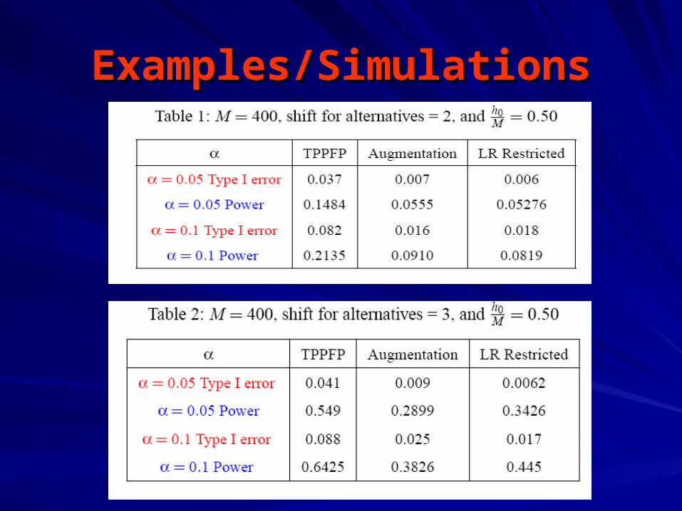
Examples/SimulationsExamples/Simulations

Summary Summary

Quantile function transformed bootstrap null distribution for test-statistics is Quantile function transformed bootstrap null distribution for test-statistics is generally valid and powerful in practice.generally valid and powerful in practice.Powerful Emp Bayes/Bootstrap Based method sharply controlling proportion Powerful Emp Bayes/Bootstrap Based method sharply controlling proportion of false positives among rejections.of false positives among rejections.Combining general bootstrap quantile null distribution for test statistics with Combining general bootstrap quantile null distribution for test statistics with random guess of true nulls provides general method for obtaining powerful random guess of true nulls provides general method for obtaining powerful (joint) multiple testing procedures (alternative to step down/up methods).(joint) multiple testing procedures (alternative to step down/up methods).Combining data adaptive regression with testing and permutation Combining data adaptive regression with testing and permutation distribution provides powerful test for independence between collection of distribution provides powerful test for independence between collection of variables and outcome.variables and outcome.Combining permutation marginal distribution with quantile transformed joint Combining permutation marginal distribution with quantile transformed joint bootstrap null distribution provides powerful valid null distribution if the null bootstrap null distribution provides powerful valid null distribution if the null hypotheses are tests of independence.hypotheses are tests of independence.Targeted ML estimation of variable importance in prediction allows multiple Targeted ML estimation of variable importance in prediction allows multiple testing (and inference) of variable importance for each variable.testing (and inference) of variable importance for each variable.

AcknowledgementsAcknowledgements

Sandrine Dudoit, for slides on MTPSandrine Dudoit, for slides on MTP

Maya PetersenMaya Petersen

Merrill BirknerMerrill Birkner

Alan HubbardAlan Hubbard