Embed Size (px)
Citation preview

On Synchronization ofElectromechanical
Hindmarsh-Rose Oscillators
E. Steur
DCT 2007.119
Master’s thesis
Coaches: Prof. dr. H. Nijmeijerir. L. Kodde
Supervisor: Prof. dr. H. Nijmeijer
Committee: Prof. dr. H. NijmeijerProf. dr. ir. P.P. Jonkerdr. A.Y. Pogromskydr. I. Tyukin (University of Leicester)ir. L. Kodde
Eindhoven University of TechnologyDepartment of Mechanical EngineeringDynamics and Control Group
Eindhoven, September, 2007


Summary
In the processing of information in our brains single neurons play an important role. Manymodels that mimic the behavior of these single neurons are introduced over the years. Ex-amples of neuronal models are the celebrated Hodgkin-Huxley equations and the well-knownHindmarsh-Rose model. Furthermore it is known that neurons do show synchronized behav-ior in several parts of the brain for various reasons.
The objective of this study to investigate the Hindmarsh-Rose model and the synchroniza-tion of Hindmarsh-Rose neurons both analytically and experimentally.
In the first place the specific behavior of the Hindmarsh-Rose neuronal model is investigatedin detail. The emerge of the typical orbits of the system are explained using fast-slow analysis.A fast subsystem gives rise to periodic orbits which, in turn, are perturbed by a slow subsys-tem. Furthermore it is shown that the motion of the Hindmarsh-Rose model can be chaotic.The existence of horseshoe type dynamics imply that there is aperiodic long term motion and,in addition, a positive Lyapunov exponent indicates that the trajectories are sensitive for ini-tial conditions. An elaborate explanation of the particular mechanisms behind this chaos isprovided by means of Poincaré maps.
To carry out the experimental part the equations of the Hindmarsh-Rose model are translatedinto an electronic equivalent. The outputs that are generated by this experimental electrome-chanical neuron do look pretty much like the outputs of the model. However, there are somesmall differences between the signals. In order to quantify these differences identification ofthe circuit is performed using the prediction error identification method and extended Kalmanfiltering. From this identification it is found that the difference in outputs is due to slight dif-ferences in the parameters of the model and its realization.
Next, the synchronization proporties of mutually coupled Hindmarsh-Rose systems are dis-covered using the semi-passivity framework. It is shown that the Hindmarsh-Rose model sat-isfies all conditions of this framework such that synchronization can be guaranteed. It is alsoshown that under certain conditions partial synchronization regimes exist.
The synchronization is investigated further for various network topologies by means ofsimulations and an experimental setup with the electromechanical Hindmarsh-Rose neurons.In all cases both the simulations as well as the experiments confirm the analytically obtainedresults.
i

ii
Samenvatting
In the verwerking van informatie in onze hersenen is een belangrijke rol weggelegd voor indi-viduele zenuwcellen. Door de jaren heen zijn er veel modellen ontwikkeld die het specifiekegedrag van zenuwcellen nabootsen. Voorbeelden hiervan zijn het gevierde Hodgkin-Huxleymodel en het bekende Hindmarsh-Rose model. Verder is het bekend dat om verschillenderedenen zenuwcellen in bepaalde delen van de hersenen synchroon gedrag vertonen.
Het doel van deze studie is om het Hindmarsh-Rose model en de synchronisatie vanHindmarsh-Rose zenuwcellen op zowel een analytische wijze als via experimenten te onder-zoeken.
Allereerst is het Hindmarsh-Rose model in detail verkend. De typische oplossingen van hetmodel worden verklaard aan de hand van fast-slow analyse. Een snel subsysteem genereertperiodieke oplossingen. Deze oplossingen worden vervolgens verstoord worden door eenlangzaam subsysteem. Verder is aangetoond dat het Hindmarsh-Rose systeem chaotischeoplossingen kan genereren. Daarbij impliceert het bestaan van horseshoe dynamica impliceertdat er niet-periodieke oplossingen voorkomen en een positieve Lyapunov exponent toont dathet systeem gevoelig is voor verschillen in begincondities. Een uitvoerige analyse van demechanismen achter deze chaos is uitgevoerd met behulp van Poincaré mappen.
Voor het uitvoeren van het experimentele gedeelte is een elektronisch equivalent van hetHindmarsh-Rose model gemaakt. De gegenereerde signalen van deze elektromechanischezenuwcel vertonen grote gelijkenissen met de signalen van het model. Om de toch aanwezigekleine verschillen tussen beide signalen te verklaren is identificatie van het circuit uitgevo-erd door middel van prediction error identification method en extended Kalman filtering. Daaruitvolgt dat de verschillen te wijten zijn aan kleine afwijkende waarden van de parameters vanhet model en de realisatie.
Vervolgens is synchronisatie van wederzijds gekoppelde Hindmarsh-Rose systemen onder-zocht. Daarbij is het gebruik gemaakt van het semi-passivity kader voor het ontwerp van syn-chroniserende systemen. Het is aangetoond dat alle condities die aan de Hindmarsh-Rosesystemen gesteld worden zijn voldaan zodat synchroon gedrag gegarandeerd kan worden.Verder is het bestaan van gebieden van partiële synchronisatie aangegeven.
Het synchrone gedrag is verder onderzocht voor verschillende netwerk topologieën doormiddel van simulaties en experimenten met de elektromechanische zenuwcellen. Zowelde resultaten van de simulaties als de experimentele resultaten ondersteunen de analytischverkregen resultaten.
iii

iv
Contents
1 Introduction 11.1 Neuronal oscillators . . . . . . . . . . . . . . . . . . . 11.2 Chaos . . . . . . . . . . . . . . . . . . . . . . . 31.3 Synchronization . . . . . . . . . . . . . . . . . . . . 41.4 Objectives . . . . . . . . . . . . . . . . . . . . . . 51.5 Outline . . . . . . . . . . . . . . . . . . . . . . . 61.6 Nomenclature . . . . . . . . . . . . . . . . . . . . . 6
2 The Hindmarsh-Rose neuronal model 92.1 Historical notes . . . . . . . . . . . . . . . . . . . . 92.2 The Hindmarsh-Rose dynamics . . . . . . . . . . . . . . . 11
2.2.1 Preliminaries . . . . . . . . . . . . . . . . . . 122.2.2 The responsible mechanisms for generation of the flows . . . . 142.2.3 The Bifurcation diagram . . . . . . . . . . . . . . . 15
2.3 Hindmarsh-Rose chaotic dynamics . . . . . . . . . . . . . . 172.3.1 The horseshoe map . . . . . . . . . . . . . . . . 202.3.2 Lyapunov exponents . . . . . . . . . . . . . . . . 212.3.3 Period doubling, saddle-node bifurcations and intermittent chaos . 22
2.4 Summary . . . . . . . . . . . . . . . . . . . . . . 25
3 Realization and identification of the electromechanical neuron 293.1 Realization . . . . . . . . . . . . . . . . . . . . . . 293.2 Experiments . . . . . . . . . . . . . . . . . . . . . 323.3 Identification . . . . . . . . . . . . . . . . . . . . . 32
3.3.1 Identification of the slow subsystem . . . . . . . . . . . 323.3.2 Identification of the fast subsystem . . . . . . . . . . . 343.3.3 Results . . . . . . . . . . . . . . . . . . . . 37
3.4 Discussion . . . . . . . . . . . . . . . . . . . . . . 383.5 Summary . . . . . . . . . . . . . . . . . . . . . . 40
4 Synchronization of Hindmarsh-Rose neurons: General theory 414.1 Preliminaries . . . . . . . . . . . . . . . . . . . . . 41
4.1.1 Passive systems . . . . . . . . . . . . . . . . . . 424.1.2 Convergent systems . . . . . . . . . . . . . . . . 43
4.2 Sufficient conditions for synchronization . . . . . . . . . . . . 44
v

Contents
4.3 Partial synchronization . . . . . . . . . . . . . . . . . . 464.4 Synchronization robustness . . . . . . . . . . . . . . . . 474.5 Synchronization and graph topology . . . . . . . . . . . . . 49
4.5.1 Wu-Chua conjecture . . . . . . . . . . . . . . . . 504.5.2 Connection Graph Stability (CGS) method . . . . . . . . . 504.5.3 Example . . . . . . . . . . . . . . . . . . . . 50
4.6 Summary . . . . . . . . . . . . . . . . . . . . . . 52
5 Synchronization of Hindmarsh-Rose neurons: Simulations and experiments 535.1 Preliminaries . . . . . . . . . . . . . . . . . . . . . 535.2 Two systems . . . . . . . . . . . . . . . . . . . . . 545.3 Three systems . . . . . . . . . . . . . . . . . . . . . 555.4 Four systems . . . . . . . . . . . . . . . . . . . . . 55
5.4.1 Full synchronization . . . . . . . . . . . . . . . . 565.4.2 Partial synchronization . . . . . . . . . . . . . . . 58
5.5 Summary . . . . . . . . . . . . . . . . . . . . . . 61
6 Conclusions and recommendations 636.1 Conclusions . . . . . . . . . . . . . . . . . . . . . 636.2 Recommendations . . . . . . . . . . . . . . . . . . . 64
Bibliography 67
A The Approximated 1D Poincaré Map 73
B Proof of Propositions 75B.1 Proof of Proposition 4.2.2 . . . . . . . . . . . . . . . . . 75B.2 Proof of Proposition 4.2.4 . . . . . . . . . . . . . . . . . 76B.3 Proof of Proposition 4.4.1 . . . . . . . . . . . . . . . . . 77
C Electrical circuits 81C.1 The electromechanical Hindmarsh-Rose neuron . . . . . . . . . 81C.2 Interface board . . . . . . . . . . . . . . . . . . . . 85
D Identification of the circuit 87
E Additional measurements 91E.1 Single circuit . . . . . . . . . . . . . . . . . . . . . 91
E.1.1 Constant inputs . . . . . . . . . . . . . . . . . . 91E.1.2 Step responses . . . . . . . . . . . . . . . . . . 94
E.2 Synchronizing circuits . . . . . . . . . . . . . . . . . . 95E.2.1 Full synchronization . . . . . . . . . . . . . . . . 95E.2.2 Partial synchronization . . . . . . . . . . . . . . . 99
F Selected Papers 101
vi

vii

viii
Chapter 1
Introduction
This chapter introduces first the three major subjects of this thesis, namely neuronal oscilla-tors, chaotic systems and synchronization. Next a the objectives of this research are coinedand the structure of the thesis is presented. Finally the necessary notations that are used inthe report are given.
1.1 Neuronal oscillators
It is well known that single neurons are important functional units for the computationalproporties of brain (Koch, 1999; Bullock et al., 2005). The most important physical variablein neural computation is the neurons membrane potential, denoted by Vm, which can rapidlychange and which controls a vast number of ionic channels. These channels, in most cases,change by the release and reception of neurotransmitters the membrane potential of otherneurons.
In general there are three states in which the membrane potential can be classified:
i. resting: In the case that there are no stimuli, e.g. reception of neurotransmitters, mostneurons are at rest, i.e. the net ionic current flowing across the neurons membrane iszero and the membrane potential is constant. All neurons have negative resting poten-tial, typically between −90 mV and −30 mV .
ii. tonic spiking: When a single neuron is stimulated its membrane potential will change.First, due to the presence of excitatory ionic currents, the membrane potential startsto become more positive. At some point inhibitory ionic currents will dominate theexcitatory currents and the membrane potential starts to decrease. The result is anaction potential or spike. In the case the neuron is tonically spiking the neurons producesuccessive action potentials. This type of output is depicted in Figure 1.1(a).
iii. bursting: Some stimulated neurons produce bursts instead of spike trains. In the burst-ing mode the neuron shows a number of spikes followed by some relatively long periodof quiescence. This bursting mode is shown in Figure 1.1(b). The case that the numberof spikes per bursts is irregular, see Figure 1.1(c), will be referred to as chaotic bursting.
Since the introduction of clamping techniques which made it possible to measure themembrane potential of single neurons (Koch, 1999), and inspired by the pioneering works
1

1. Introduction
t
Vm
(a) Tonic spiking
t
Vm
(b) bursting
t
Vm
(c) chaotic bursting
Figure 1.1: Different types of fluctuations of the membrane potential Vm.
by Hodgkin and Huxley (Hodgkin and Huxley, 1952), a large number of models describingthe dynamical changes in membrane potential of neural cells have been developed, see forinstance (Izhikevich, 2000).
In general, models of neural dynamics can be classified as biophysically plausible or aspurely mathematical. The biophysically plausible conductance based neuronal models de-scribe the generation of the action potentials as function of the individual ionic currents flow-ing through the neuron’s membrane. The biophysically plausible models are of the form:
CVm =N∑
j=1
Ij(Vm),
or, in terms of conductances,
CVm =N∑
j=1
gj(Vm) · (Vm − Vj) ,
where C is the membrane capacity, Ij(Vm) are the membrane potential dependent ionic cur-rents with j = 1, . . . , N denoting the number of different ionic currents, e.g. potassium orsodium currents, gj(Vm) are the membrane potential dependent conductances and Vj are theconstant reversal potentials. Examples of biophysically plausible models are the celebratedHodgkin-Huxley equations and the Morris-Lecar model (Morris and Lecar, 1981).
Since the biophysically based models are extremely costly to evaluate computationally,a number of mathematical models that mimic the spiking behavior of real neurons havebeen introduced over the years, e.g. the Hindmarsh-Rose (Hindmarsh and Rose, 1984) andFitzhugh-Nagumo (FitzHugh, 1961) neuronal models. These models consist of coupled non-linear differential equations:
x1 = f1(x, u),x2 = f2(x),
...xn = fn(x),
where the states x ∈ Rn, input u ∈ R and functions f1 : Rn × R → R, fi : Rn → R,i = 2, . . . , n. The state x1 represents in this case the membrane potential. It is showed byIzhikevich (Izhikevich, 2000) that these models can, depending on their specific parameters,cover a wide range of the dynamics that are observed in real neurons.
2
1.2 Chaos
Even more simple models of spiking behavior exist, i.e. the class of integrate and firemodels (Koch, 1999). These models consist of one or two (unstable) differential equationswhose states are reset after some preset threshold is reached. Although these models do notoffer a realistic description of the membrane potential they are often used for the investigationof cooperative behavior in complex or large neural networks, see (Gong and van Leeuwen,2007) for instance.
1.2 Chaos
Chaotic behavior of a system refers to the case when a deterministic system shows compli-cated motion depending on the initial conditions. Chaos theory is probably first described bythe French mathematician Henri Poincaré, who in the end of the nineteenth century showedthat the behavior of orbits of three celestial bodies arising from different sets of initial con-ditions could be very complicated (Ott, 2002). In 1927, Balthasar van der Pol noticed "noisy"behavior in his well known electrical oscillator (van der Pol, 1927) and in the early 1940sCartwright and Littlewood discovered phenomena in the van der Pol equations that are nowcalled chaos (Dyson, 1996). The name chaos was coined by Jim Yorke in 1961 (Ruelle, 1991).
In the 1960s, Smale, Peixoto, Sinai, Kolmogorov, Moser and Arnol’d used topological tech-niques to understand the chaos of a large class of (hyperbolically) dynamical systems. EdwardLorenz, a meteorologist, showed in 1963, based on a computer study, sensitive dependenceon initial conditions and complex motion in a very simplified model of convection rolls in theatmosphere. However, the findings of Lorenz were not very much appreciated at that timesince they imply that long-term prediction of the weather is not possible. Attention to thefamous Lorenz system will be given in somewhat later on.
In 1971 David Ruelle and Floris Takens published their famous paper "On the Nature ofTurbulence" and introduced the term strange attractor (Ruelle and Takens, 1971). In the mid1970s May found chaotic behavior arising from period doubling bifurcations in iterated mapsdescribing insect populations, and, a few years later, Feigenbaum discovered that there arecertain universal laws governing the transition from regular motion to chaotic motion (Stro-gatz, 1994). Since the 1980s the work on chaotical dynamical systems is widespread withapplications to, for instance, the control of chaotic systems (Ott et al., 1990) or (secure) com-munication (Huijberts et al., 1998).
An example of chaotic behavior
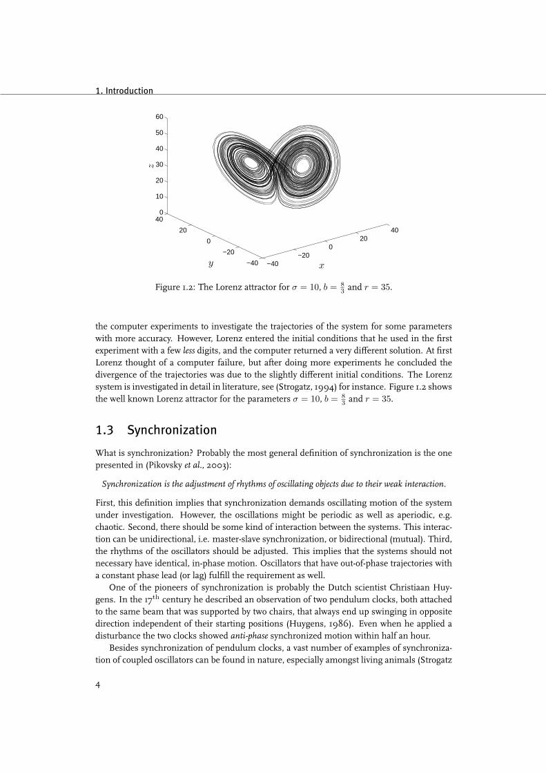
Many examples of chaotic systems can be found in literature (see (Guckenheimer andHolmes,1983; Strogatz, 1994; Ott, 2002) for instance). Here special attention is given to the famousLorenz system (Lorenz, 1963).
The Lorenz model is given by the following three differential equations:
x = σ(y − x),y = rx− y − xz,
z = −bz + xy, σ, r, b > 0.
Lorenz discovered accidently, that this system is very sensitive to the initial conditions. Atsome day Lorenz found an interesting solution generated by his system. He decided to repeat
3
1. Introduction
−40−20
020
40
−40
−20
0
20
400
10
20
30
40
50
60
xy
z
Figure 1.2: The Lorenz attractor for σ = 10, b = 83 and r = 35.
the computer experiments to investigate the trajectories of the system for some parameterswith more accuracy. However, Lorenz entered the initial conditions that he used in the firstexperiment with a few less digits, and the computer returned a very different solution. At firstLorenz thought of a computer failure, but after doing more experiments he concluded thedivergence of the trajectories was due to the slightly different initial conditions. The Lorenzsystem is investigated in detail in literature, see (Strogatz, 1994) for instance. Figure 1.2 showsthe well known Lorenz attractor for the parameters σ = 10, b = 8
3 and r = 35.
1.3 Synchronization
What is synchronization? Probably the most general definition of synchronization is the onepresented in (Pikovsky et al., 2003):
Synchronization is the adjustment of rhythms of oscillating objects due to their weak interaction.
First, this definition implies that synchronization demands oscillating motion of the systemunder investigation. However, the oscillations might be periodic as well as aperiodic, e.g.chaotic. Second, there should be some kind of interaction between the systems. This interac-tion can be unidirectional, i.e. master-slave synchronization, or bidirectional (mutual). Third,the rhythms of the oscillators should be adjusted. This implies that the systems should notnecessary have identical, in-phase motion. Oscillators that have out-of-phase trajectories witha constant phase lead (or lag) fulfill the requirement as well.
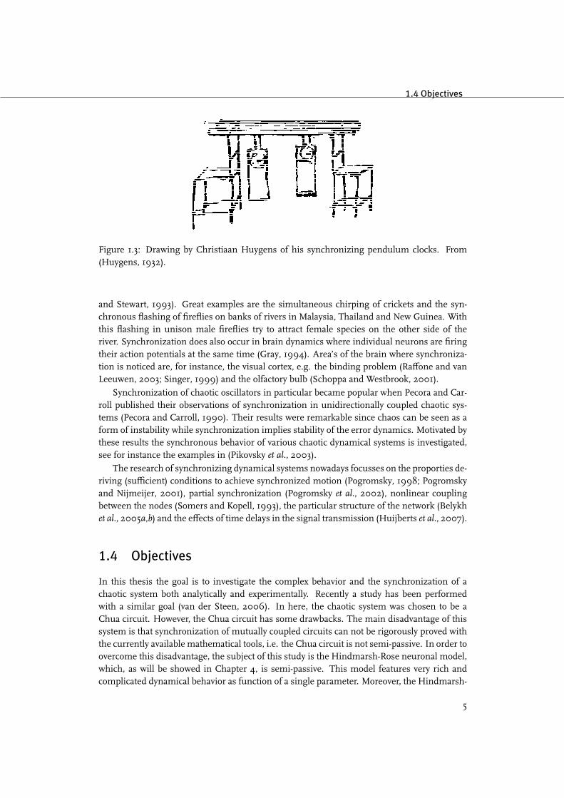
One of the pioneers of synchronization is probably the Dutch scientist Christiaan Huy-gens. In the 17th century he described an observation of two pendulum clocks, both attachedto the same beam that was supported by two chairs, that always end up swinging in oppositedirection independent of their starting positions (Huygens, 1986). Even when he applied adisturbance the two clocks showed anti-phase synchronized motion within half an hour.
Besides synchronization of pendulum clocks, a vast number of examples of synchroniza-tion of coupled oscillators can be found in nature, especially amongst living animals (Strogatz
4
1.4 Objectives
Figure 1.3: Drawing by Christiaan Huygens of his synchronizing pendulum clocks. From(Huygens, 1932).
and Stewart, 1993). Great examples are the simultaneous chirping of crickets and the syn-chronous flashing of fireflies on banks of rivers in Malaysia, Thailand and New Guinea. Withthis flashing in unison male fireflies try to attract female species on the other side of theriver. Synchronization does also occur in brain dynamics where individual neurons are firingtheir action potentials at the same time (Gray, 1994). Area’s of the brain where synchroniza-tion is noticed are, for instance, the visual cortex, e.g. the binding problem (Raffone and vanLeeuwen, 2003; Singer, 1999) and the olfactory bulb (Schoppa and Westbrook, 2001).
Synchronization of chaotic oscillators in particular became popular when Pecora and Car-roll published their observations of synchronization in unidirectionally coupled chaotic sys-tems (Pecora and Carroll, 1990). Their results were remarkable since chaos can be seen as aform of instability while synchronization implies stability of the error dynamics. Motivated bythese results the synchronous behavior of various chaotic dynamical systems is investigated,see for instance the examples in (Pikovsky et al., 2003).
The research of synchronizing dynamical systems nowadays focusses on the proporties de-riving (sufficient) conditions to achieve synchronized motion (Pogromsky, 1998; Pogromskyand Nijmeijer, 2001), partial synchronization (Pogromsky et al., 2002), nonlinear couplingbetween the nodes (Somers and Kopell, 1993), the particular structure of the network (Belykhet al., 2005a,b) and the effects of time delays in the signal transmission (Huijberts et al., 2007).
1.4 Objectives
In this thesis the goal is to investigate the complex behavior and the synchronization of achaotic system both analytically and experimentally. Recently a study has been performedwith a similar goal (van der Steen, 2006). In here, the chaotic system was chosen to be aChua circuit. However, the Chua circuit has some drawbacks. The main disadvantage of thissystem is that synchronization of mutually coupled circuits can not be rigorously proved withthe currently available mathematical tools, i.e. the Chua circuit is not semi-passive. In order toovercome this disadvantage, the subject of this study is the Hindmarsh-Rose neuronal model,which, as will be showed in Chapter 4, is semi-passive. This model features very rich andcomplicated dynamical behavior as function of a single parameter. Moreover, the Hindmarsh-
5
1. Introduction
Rose equations can be translated into an equivalent electrical circuit such that it is possible torealize an (relatively cheap) experimental setup. In brief, the main goals of the thesis are
i. to analyse the Hindmarsh-Rose model,
ii. to realize an electrical equivalent of the Hindmarsh-Rose model,
iii. to compare the behavior of the model with the experimental setup,
iv. to create a network of a couple of circuits and to synchronize these mutually coupledsystems.
1.5 Outline
This thesis is organized as follows. At the end of this chapter the reader is made familiarwith the notations used throughout this report. Chapter 2 focusses on the dynamics of theHindmarsh-Rose model. A description of the mechanism to produce the spiking and burst-ing behavior is presented. The details over the realization and identification of the electrome-chanical Hindmarsh-Rose neuron are given in Chapter 3. The next two chapters will treat thesynchronization of Hindmarsh-Rose neurons. First sufficient conditions which ensure syn-chronization are derived, and the existence of invariant linear manifold that correspond to thesynchronized state will be showed by simulations and experiments. Finally conclusions aredrawn and recommendations for future research are given.
1.6 Nomenclature
The symbol R denotes the field of real number. Let R+ stands for the following subset of R:R+ = x ∈ R | x ≥ 0. The Euclidian norm in x ∈ Rn is denoted by ‖ x ‖. The supremumnorm ‖ x ‖∞ is defined as supτ∈R+
‖ x(τ) ‖. A function α(s) is said to belong to class-K ifα : R+ → R+ is a strictly increasing function and α(0) = 0. If, in addition, lims→∞ α(s) =∞, then the function belongs to class-K∞. The function β : R+ × R+ → R+ is a class-KLfunction if β(·, 0) belongs to class-K and β(0, ·) is strictly decreasing. The composition of twofunctions f(·) and g(·) is denoted by f g(r) = f(g(r)). Let f : xk 7→ xk+1 then the nth
iterate of the map f , i.e.f . . . f︸ ︷︷ ︸
n times
(xk),
is denoted by fn(xk). Consider the vector x ∈ Rn that can be partitioned into two vectorsx1 ∈ Rp and x2 ∈ Rq, p + q = n, then ⊕ denotes their concatenation x1 ⊕ x2 = x. Thesymbol In stands for the n × n identity matrix and Jn×m stands for the n × m unit matrix.In advance, the symbol On denotes the n × n matrix with all entries equal to zero. A n × n
matrix A with only entries on the diagonal will be denoted as A = diag([a0, a1, , . . . , an])such that
A = diag([a0, a1, , . . . , an]) =
a0 0 · · · 00 a1 · · · 0...
.... . .
...0 0 · · · an
.
6

1.6 Nomenclature
For a n × n matrix A and a matrix B, the Kronecker product A ⊗ B stands for the matrixcomposed of the submatrices AijB, i.e.
A⊗B =
A11B A12B · · · A1nBA21B A22B · · · A2nB
......
. . ....
An1B An2B · · · AnnB
,
where Aij , i, j = 1, 2, . . . , n stands for the ijth entry of A.
7

1. Introduction
8

Chapter 2
The Hindmarsh-Rose neuronal model
In this chapter the dynamics of the Hindmarsh-Rose model for neuronal activity are dis-cussed. First attention is given to the development of the model. How did J.L. Hindmarshand R.M. Rose find these particular equations? The remainder of this chapter focusses on the(complex) dynamical mechanisms that allow the model to generate the spiking or burstingmembrane potential.
2.1 Historical notes
As described in (Hindmarsh and Cornelius, 2005), the development of the Hindmarsh-Rosemodel starts when J.L. Hindmarsh and R.M. Rose both participate in a project at Cardiff Uni-versity to model the synchronization of firing of two snail neurons in a relative simple waywithout the need to integrate the celebrated Hodgkin-Huxley (Hodgkin and Huxley, 1952)equations. As noticed in (Izhikevich, 2004) evaluation of the Hodgkin-Huxley model is ex-tremely costly in terms of floating point operations. Therefore it is not the most preferablemodel to investigate synchronization, certainly not with the not very powerful computer avail-able that time. The most simple models of neuronal activity known that time are of theFitzHugh-Nagumo (FitzHugh, 1961; Nagumo et al., 1962; Koch, 1999) type
x = a(y − f(x) + u(t)),y = b(g(x)− y),
where x denotes the membrane potential, y is an internal variable and a, b > 0 are timeconstants. The function f(·) is cubic, the function g(·) is linear an u(t) is the external, applied,or clamping current at time t. The main problem with these equations is that they do notoffer a realistic description of the spikes, that is the model shows rapid firing but doesn’thave a relatively long interval between two successive spikes. Several attempts are made toimprove the model’s behavior by making the constants a and b voltage dependent, but nosatisfying results are obtained. The breakthrough comes when R.M. Rose asked himself thequestion whether the FitzHugh-Nagumo equations could account for the so-called tail currentreversal. Taking the tail current reversal into account, Hindmarsh and Rose found that thefunction g(·) should be a quadratic function instead of a linear one. This small modificationof the FitzHugh-Nagumo equations did lead to the first Hindmarsh-Rosemodel, i.e. the single
9
2. The Hindmarsh-Rose neuronal model
y
x
y = 0
x = 0
xA
xB
xC
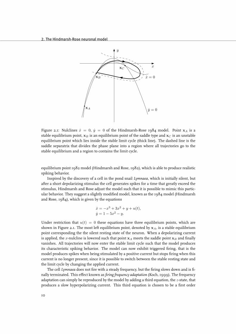
Figure 2.1: Nulclines x = 0, y = 0 of the Hindmarsh-Rose 1984 model. Point xA is astable equilibrium point, xB is an equilibrium point of the saddle type and xC is an unstableequilibrium point which lies inside the stable limit cycle (thick line). The dashed line is thesaddle separatrix that divides the phase plane into a region where all trajectories go to thestable equilibrium and a region to contains the limit cycle.
equilibrium point 1982 model (Hindmarsh and Rose, 1982), which is able to produce realisticspiking behavior.
Inspired by the discovery of a cell in the pond snail Lymnaea, which is initially silent, butafter a short depolarizing stimulus the cell generates spikes for a time that greatly exceed thestimulus, Hindmarsh and Rose adjust the model such that it is possible to mimic this partic-ular behavior. They suggest a slightly modified model, known as the 1984 model (Hindmarshand Rose, 1984), which is given by the equations
x = −x3 + 3x2 + y + u(t),y = 1− 5x2 − y.
Under restriction that u(t) = 0 these equations have three equilibrium points, which areshown in Figure 2.1. The most left equilibrium point, denoted by xA, is a stable equilibriumpoint corresponding the the silent resting state of the neuron. When a depolarizing currentis applied, the x-nulcline is lowered such that point xA meets the saddle point xB and finallyvanishes. All trajectories will now enter the stable limit cycle such that the model producesits characteristic spiking behavior. The model can now exhibit triggered firing, that is themodel produces spikes when being stimulated by a positive current but stops firing when thiscurrent is no longer present, since it is possible to switch between the stable resting state andthe limit cycle by changing the applied current.
The cell Lymnaea does not fire with a steady frequency, but the firing slows down and is fi-nally terminated. This effect known as firing frequency adaptation (Koch, 1999). The frequencyadaptation can simply be reproduced by the model by adding a third equation, the z-state, thatproduces a slow hyperpolarizing current. This third equation is chosen to be a first order
10
2.2 The Hindmarsh-Rose dynamics
differential equation that is a linear function of x. The full set of equations is now given by
x = −x3 + 3x2 + y + u(t)− z,
y = 1− 5x2 − y,
z = r (s (x− x0)− z) ,
where r, s are positive constant parameters (r 1) and constant x0 is the x component ofthe stable equilibrium point xA when no input is applied, i.e u(t) = 0. These last equationsare often used to study synchronization of coupled oscillators, see for instance (Oud et al.,2004; Belykh et al., 2005a), and it is shown that for a suitable choice of the parameters r, s
the model can show chaotic bursting behavior (Wang, 1993; Holden and Fan, 1992a,b,c).
2.2 The Hindmarsh-Rose dynamics
Throughout the years the Hindmarsh-Rose model for neural activity and neuronal models ingeneral are analyzed extensively. The complex mechanisms behind the bursting and spikingoscillations of general cell models are explained in (Terman, 1991, 1992) and (Belykh et al.,2000). The general approach in these publications is to divide the system dynamics into a fastsubsystem that gives rise to periodic oscillations and a slow subsystemwhich is responsible forthe bursting phenomena. The complex behavior of the Hindmarsh-Rose model in particularis treated in (Holden and Fan, 1992a,b,c) and (Wang, 1993), where the focus is mainly on thetransition from bursting to spiking dynamics. In (Milne and Chalabi, 2001) control analysis ofthe Hindmarsh-Rose equations is performed in order to let the model follow desired patternsof membrane potential discharge.
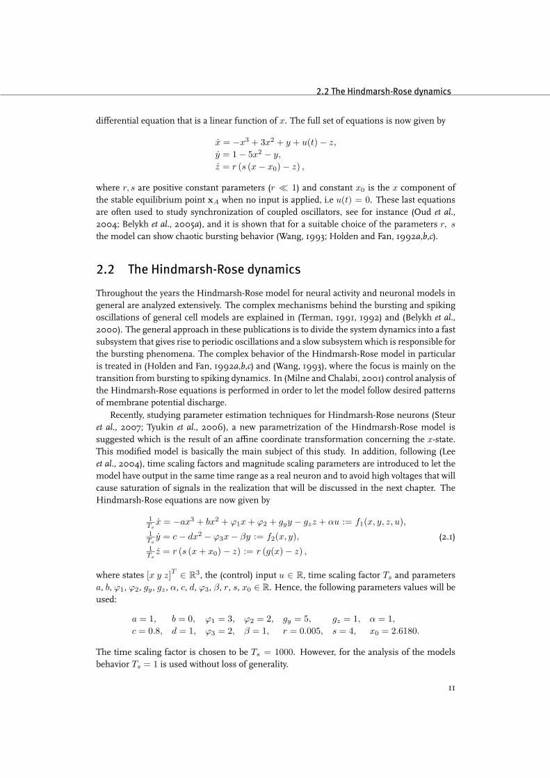
Recently, studying parameter estimation techniques for Hindmarsh-Rose neurons (Steuret al., 2007; Tyukin et al., 2006), a new parametrization of the Hindmarsh-Rose model issuggested which is the result of an affine coordinate transformation concerning the x-state.This modified model is basically the main subject of this study. In addition, following (Leeet al., 2004), time scaling factors and magnitude scaling parameters are introduced to let themodel have output in the same time range as a real neuron and to avoid high voltages that willcause saturation of signals in the realization that will be discussed in the next chapter. TheHindmarsh-Rose equations are now given by
1Ts
x = −ax3 + bx2 + ϕ1x + ϕ2 + gyy − gzz + αu := f1(x, y, z, u),1Ts
y = c− dx2 − ϕ3x− βy := f2(x, y),1Ts
z = r (s (x + x0)− z) := r (g(x)− z) ,
(2.1)
where states [x y z]T ∈ R3, the (control) input u ∈ R, time scaling factor Ts and parametersa, b, ϕ1, ϕ2, gy , gz , α, c, d, ϕ3, β, r, s, x0 ∈ R. Hence, the following parameters values will beused:
a = 1, b = 0, ϕ1 = 3, ϕ2 = 2, gy = 5, gz = 1, α = 1,
c = 0.8, d = 1, ϕ3 = 2, β = 1, r = 0.005, s = 4, x0 = 2.6180.
The time scaling factor is chosen to be Ts = 1000. However, for the analysis of the modelsbehavior Ts = 1 is used without loss of generality.
11

2. The Hindmarsh-Rose neuronal model
Figure 2.2 shows simulation results of the model for different inputs u. For each input thefigure on the left pane shows the trajectories x(t), y(t) and z(t) as function of the time, wherethe figures on the right depict the corresponding attractor. In Figure 2.2(a), the model showssuccessive burst containing two spikes when the input u = 2 is applied. If u is increased tou = 3.25, which is shown in Figure 2.2(b), the number of spikes per burst becomes irregularand the trajectories of x(t), y(t) and z(t) are sensitive for the initial conditions, i.e. the modelproduces chaotic bursts. For higher inputs the output is in the tonic spiking regime. This isdepicted in Figure 2.2(c) where an input of u = 5 is applied.
2.2.1 Preliminaries
In this section some general proporties of the Hindmarsh-Rose model are presented that arenecessary to explain the bursting and tonic spiking behavior. The following proporties holdfor (2.1) (Belykh et al., 2000):
i. The union of equilibrium points given by the equilibrium conditions f1(x, y, z, u) = 0and f2(x, y) = 0 of the system (2.1) gives a smooth, S-shaped curve S which can bedescribed by the function
z = ρ(x, u).
An additional equilibrium condition that follows from the third equation in (2.1) is givenby the function
z = g(x).
Moreover, there exists an unique equilibrium point xe = (xe, ye, ze) which is specifiedby the intersection of ρ(x, u) and g(x).
ii. There exists two critical points xc1 and xc
2 such that
dρdx (x, u) > 0 for xc
1 < x < xc2,
dρdx (x, u) < 0 for x < xc
1, x > xc2.
These two points divide the curve S into three branches: the lower branch, the middlebranch and the upper branch.
iii. There exist values xH1 , xH2 such that the divergence of the vector fieldF (f1, f2) changessign, i.e.
σ(x) := ∇ · F |z=ρ(x,u) > 0, ∀ xH1 < x < xH2 ,
σ(x) < 0, ∀ x < xH1 , x > xH2 .
The points xH1 , xH2 correspond to a pair of Andronov-Hopf bifurcations.
Evaluation of the eigenvalues of the linearization of (2.1) around the equilibrium points showsthe point located on the lower branch are stable, the equilibrium points in the middle branchare of the saddle type and the points in upper branch are unstable (stable) for x < xH2 (x >
xH2 , respectively).
Consider the systemξ = F (ξ, z, u), z = const, (2.2)
12
2.2 The Hindmarsh-Rose dynamics
0 0.2 0.4 0.6 0.8 1
−2
−1
0
x[V
]
0 0.2 0.4 0.6 0.8 1−10
−5
0
y[V
]
0 0.2 0.4 0.6 0.8 11.6
1.8
2
2.2
time [s]
z[V
]
−10
−5
0
−2
−1
0
1.7
1.8
1.9
2
2.1
y [V ]x [V ]
z[V
]
(a) bursting
0 0.2 0.4 0.6 0.8 1−2
−1
0
x[V
]
0 0.2 0.4 0.6 0.8 1
−6−4−2
0
y[V
]
0 0.2 0.4 0.6 0.8 1
3
3.5
time [s]
z[V
]
−6−4
−20
−2
−1
0
2.9
3
3.1
3.2
3.3
y [V ]x [V ]
z[V
]
(b) chaotic bursting
0 0.05 0.1 0.15 0.2−2
−1
0
x[V
]
0 0.05 0.1 0.15 0.2−6
−4
−2
0
y[V
]
0 0.05 0.1 0.15 0.24.7
4.8
4.9
time [s]
z[V
]
−6−4
−20
−1.5−1
−0.50
0.5
4.75
4.76
4.77
4.78
4.79
y [V ]x [V ]
z[V
]
(c) spiking
Figure 2.2: Some simulated responses of the Hindmarsh-Rose model for different inputs u.
13
2. The Hindmarsh-Rose neuronal model
where ξ = [x, y]T and F (f1, f2). This system is the fast subsystem of (2.1). Dependent on
the values of z and u the system (2.2) has a limit cycle JO =
[x, y]T = ξ(t, z, u)of period
τ(z) = 2πω(z) and, in additional, there exist a saddle type equilibrium point Oh that has a
homoclinic orbit HO. Then, according to Theorem 2 from (Belykh et al., 2000), given that0 < r 1, the equilibrium point Oh of the system (2.1) has a homoclinic orbitH close toHO.
Lemma 2.2.1. (Belykh et al., 2000) Let
κ(z) =1
τ(z)
τ(z)∫0
∇F (ξ(t, z, u))dt 6= 0.
Then the system (2.1) has a cylindrical manifoldM =
[x, y]T = ξ(t, z, u)stable for κ < 0 and
unstable for κ > 0.
Lemma 2.2.2. (Belykh et al., 2000) Given the integral
I(z) =1
τ(z)
τ(z)∫0
(g (ξ (t, z, u))− z) dt,
if I(z) 6= 0, then the manifoldM is transient for the flow of (2.1). Namely, for I(z) < 0 (> 0) alltrajectories inM are rotating in decreasing (increasing, respectively) direction of z.
Definition 2.2.1. The solution of (2.1) on the time interval [t0, t1] is described by x(t) = φ(t),where the flow φ : R+ → R3, x = [x, y, z]T and t ∈ [t0, t1].
2.2.2 The responsible mechanisms for generation of the flows
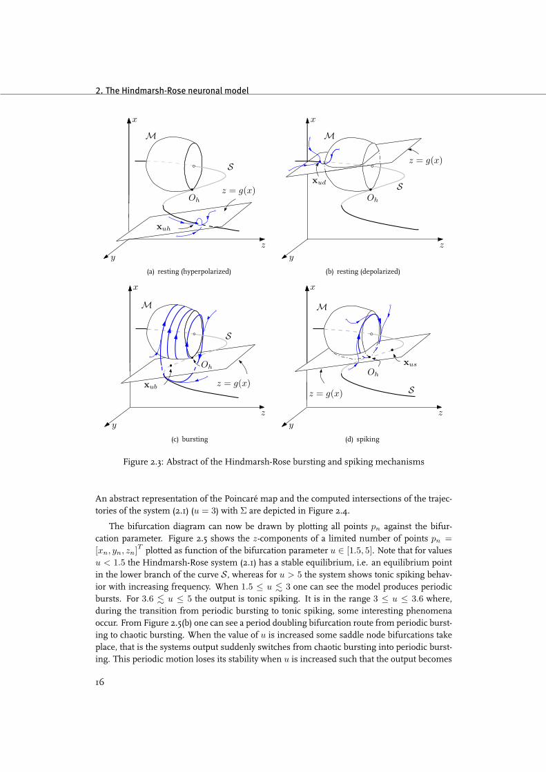
The Hindmarsh-Rose model can operate, like a vast number of neuronal models, in threedifferent modes: (i) resting, (ii) bursting and (iii) tonic spiking. Given the conditions as pre-sented in the previous section, the mechanisms responsible for these modes can be readilyexplained. Supporting pictures are showed in Figure 2.3.
Resting
The most easy mode to explain is resting. The term resting refers to either the hyperpolarizedor depolarized state of the neuron (Cymbalyuk et al., 2005). In the case of hyperpolarization,u . 1.5, the intersection of the function z = g(x) with the function z = ρ(x, u) is in the lowerbranch of the curve S, and will thus define an stable unique equilibrium point denoted byxuh. This means that every (perturbed) flow φ(t) for every initial condition φ(t0) ends up atthe point xuh. A geometrical representation can be found in Figure 2.3(a). When the systemis depolarized, the intersection g(x) ∩ ρ(x, u) defines a stable equilibrium point xud in theupper branch of S, left of the Hopf bifurcation point xH2 , see Figure 2.3(b). This equilibriumpoint only exist for large values u & 24.
14
2.2 The Hindmarsh-Rose dynamics
Bursting
In the bursting region the functions z = g(x) and z = ρ(x, u) intersect in the middle branchof S, left of the homoclinic pointOh, and define the equilibrium point denoted by xub. Follow-ing (Terman, 1991), a point φ(t0) is taken somewhere near the lower branch of the curve S. Inthis region themovement of the flow is dominated by the slow dynamics. Since g(φ(t))−z < 0the flow will move slowly up to the left most knee of S, i.e. the critical point xc
1. At this point,a fold bifurcation occurs, and φ(t) will enter the cylindrical manifoldM, which is stable sinceκ(z) < 0. Because now I(z) > 0, the flow will loop around M and move in increasingz-direction until it reaches the homoclinic point Oh. At this point, a homoclinic bifurcationoccurs, that forces the flow back to the lower branch and let the whole process start over andover again. See Figure 2.3(c) for the geometrical explanation.
Tonic spiking
Due to the fact a larger input u is applied, the intersection of the functions g(x) and ρ(x, u)defines an equilibrium point xus that is located at the unstable middle branch of S, right ofthe homoclinic point Oh. As can be seen in Figure 2.3(d) the surface described by z = g(x)divides the homoclinic orbit H near the saddle Oh into two pieces (Belykh et al., 2000). Takea point φ(t0) on the stable, κ(z) < 0, manifoldM such that g(φ(t)) > z. In this region theintegral I(z) > 0 such that the flow φ(t) moves in increasing z-direction. Then the flow willenter the region where g(φ(t)) < z, and since here the integral I(z) < 0, the movement ofthe flow is in decreasing z-direction. This means the flow falls back to the vicinity of the pointOh such that the system (2.1) has a stable limit cycle on the manifoldM. This corresponds tothe tonic spiking mode.
2.2.3 The Bifurcation diagram
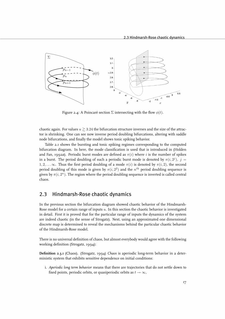
To investigate how the Hindmarsh-Rose system (2.1) exactly responds on a certain input u thebifurcation diagram will be computed. The bifurcation diagram shows the long term motionof the system as function of the bifurcation parameter, here the input u. The bifurcationdiagram will be obtained by calculating the intersections of the trajectories of the systems(2.1) with a plane, i.e. a Poincaré map.
Consider again the flow φ(t) as the solution of the system (2.1). A local cross section, thePoincaré section, Σ ∈ R2 is taken such that that flow φ(t) is everywhere transverse to it. Like(Holden and Fan, 1992a) a section through the unique equilibrium point of (2.1) is chosen:
Σ =(x, y, z) ∈ R3|x > −1.5, (−0.135− yeq)(x− xeq) + (0.005 + xeq)(y − yeq) = 0
,
which is parallel to the z-axis. Let p0 be the point on Σ where the flow φ(t) intersects with Σ,then the Poincaré map P is the mapping from Σ to itself, i.e. P : Σ 7→ Σ. Thus starting at apoint p0 on Σ, the Poincaré map will define the next intersection p1 of the flow φ(t) with Σ.This is called the first return map. Starting from point p1, the second intersection of the flowwith Σ gives the point p2.The complete map is thus defined as
P : pn 7→ pn+1, n = 0, . . . ,∞.
15
2. The Hindmarsh-Rose neuronal model
x
y
z
Oh
M
S
xuh
z = g(x)
(a) resting (hyperpolarized)
x
y
z
Oh
M
Sxud
z = g(x)
(b) resting (depolarized)
x
y
z
xub z = g(x)
Oh
S
M
(c) bursting
x
y
z
xus
z = g(x)
Oh
S
M
(d) spiking
Figure 2.3: Abstract of the Hindmarsh-Rose bursting and spiking mechanisms
An abstract representation of the Poincaré map and the computed intersections of the trajec-tories of the system (2.1) (u = 3) with Σ are depicted in Figure 2.4.
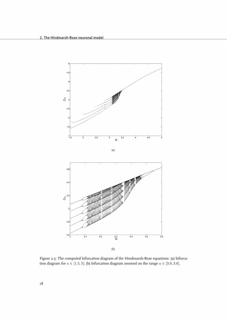
The bifurcation diagram can now be drawn by plotting all points pn against the bifur-cation parameter. Figure 2.5 shows the z-components of a limited number of points pn =[xn, yn, zn]T plotted as function of the bifurcation parameter u ∈ [1.5, 5]. Note that for valuesu < 1.5 the Hindmarsh-Rose system (2.1) has a stable equilibrium, i.e. an equilibrium pointin the lower branch of the curve S, whereas for u > 5 the system shows tonic spiking behav-ior with increasing frequency. When 1.5 ≤ u . 3 one can see the model produces periodicbursts. For 3.6 . u ≤ 5 the output is tonic spiking. It is in the range 3 ≤ u ≤ 3.6 where,during the transition from periodic bursting to tonic spiking, some interesting phenomenaoccur. From Figure 2.5(b) one can see a period doubling bifurcation route from periodic burst-ing to chaotic bursting. When the value of u is increased some saddle node bifurcations takeplace, that is the systems output suddenly switches from chaotic bursting into periodic burst-ing. This periodic motion loses its stability when u is increased such that the output becomes
16
2.3 Hindmarsh-Rose chaotic dynamics
Σ
pn−1
pn
pn+1
φ(t)
Figure 2.4: A Poincaré section Σ intersecting with the flow φ(t).
chaotic again. For values u & 3.24 the bifurcation structure inverses and the size of the attrac-tor is shrinking. One can see now inverse period doubling bifurcations, altering with saddlenode bifurcations, and finally the model shows tonic spiking behavior.
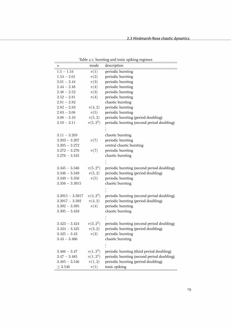
Table 2.1 shows the bursting and tonic spiking regimes corresponding to the computedbifurcation diagram. In here, the mode classification is used that is introduced in (Holdenand Fan, 1992a). Periodic burst modes are defined as π(i) where i is the number of spikesin a burst. The period doubling of such a periodic burst mode is denoted by π(i, 2j), j =1, 2, . . .∞. Thus the first period doubling of a mode π(i) is denoted by π(i, 2), the secondperiod doubling of this mode is given by π(i, 22) and the nth period doubling sequence isgiven by π(i, 2n). The region where the period doubling sequence is inverted is called centralchaos.
2.3 Hindmarsh-Rose chaotic dynamics
In the previous section the bifurcation diagram showed chaotic behavior of the Hindmarsh-Rose model for a certain range of inputs u. In this section the chaotic behavior is investigatedin detail. First it is proved that for the particular range of inputs the dynamics of the systemare indeed chaotic (in the sense of Strogatz). Next, using an approximated one dimensionaldiscrete map is determined to reveal the mechanisms behind the particular chaotic behaviorof the Hindmarsh-Rose model.
There is no universal definition of chaos, but almost everybody would agree with the followingworking definition (Strogatz, 1994):
Definition 2.3.1 (Chaos). (Strogatz, 1994) Chaos is aperiodic long-term behavior in a deter-ministic system that exhibits sensitive dependence on initial conditions:
i. Aperiodic long term behavior means that there are trajectories that do not settle down tofixed points, periodic orbits, or quasiperiodic orbits as t →∞,
17
2. The Hindmarsh-Rose neuronal model
(a)
(b)
Figure 2.5: The computed bifurcation diagram of the Hindmarsh-Rose equations: (a) bifurca-tion diagram for u ∈ [1.5, 5]; (b) bifurcation diagram zoomed on the range u ∈ [3.0, 3.6].
18
2.3 Hindmarsh-Rose chaotic dynamics
Table 2.1: bursting and tonic spiking regimes
u mode description
1.5− 1.54 π(1) periodic bursting1.54− 2.01 π(2) periodic bursting2.01− 2.44 π(3) periodic bursting2.44− 2.48 π(4) periodic bursting2.48− 2.52 π(3) periodic bursting2.52− 2.81 π(4) periodic bursting2.81− 2.82 chaotic bursting2.82− 2.83 π(4, 2) periodic bursting2.83− 3.08 π(5) periodic bursting3.08− 3.10 π(5, 2) periodic bursting (period doubling)3.10− 3.11 π(5, 22) periodic bursting (second period doubling)
...3.11− 3.203 chaotic bursting3.203− 3.207 π(7) periodic bursting3.205− 3.272 central chaotic bursting3.272− 3.276 π(7) periodic bursting3.276− 3.345 chaotic bursting
...3.345− 3.346 π(5, 22) periodic bursting (second period doubling)3.346− 3.349 π(5, 2) periodic bursting (period doubling)3.349− 3.356 π(5) periodic bursting3.356− 3.3915 chaotic bursting
...3.3915− 3.3917 π(4, 22) periodic bursting (second period doubling)3.3917− 3.392 π(4, 2) periodic bursting (period doubling)3.392− 3.395 π(4) periodic bursting3.395− 3.433 chaotic bursting
...3.423− 3.424 π(3, 22) periodic bursting (second period doubling)3.424− 3.425 π(3, 2) periodic bursting (period doubling)3.425− 3.43 π(3) periodic bursting3.43− 3.466 chaotic bursting
...3.466− 3.47 π(1, 23) periodic bursting (third period doubling)3.47− 3.485 π(1, 22) periodic bursting (second period doubling)3.485− 3.546 π(1, 2) periodic bursting (period doubling)≥ 3.546 π(1) tonic spiking
19

2. The Hindmarsh-Rose neuronal model
A B
CD
H H
A B
CD
H1
H2
V1 V2
H H
H1
Figure 2.6: The horseshoe.
ii. Deterministic means that the system has no random or noisy inputs or parameters suchthat irregular behavior is completely due to the system dynamics, and
iii. Sensitive dependence on initial conditionsmean that nearby trajectories separate exponen-tially fast.
It follows immediately from the system dynamics that (ii) of Definition 2.3.1 is satisfied.In the next two subsection the two other proporties of a chaotic system are investigated.
2.3.1 The horseshoe map
For equilibrium points near the homoclinic point, the dynamics of the system (2.1) are of thehorseshoe type (Belykh et al., 2005c; Xie et al., 2004). A proof for this can be found in (Ter-man, 1991).
The horseshoe, introduced by Smale (Smale, 1967), is a hyperbolic limit set that provides a ba-sis for understanding a large class of chaotic dynamical systems (Guckenheimer and Holmes,1983). Let S be the unit square [0 1] × [0 1] and define the mapping H : S → R2. Thismapping stretches S in vertical direction and compresses S in horizontal direction by factorsµv > 2 and 0 < µh < 1
2 , respectively. S is now long and thin. Next, S is folded in put backinside S, which is showed in Figure 2.6. One can easily see that H(S) ∩ S consist of twovertical stripes V1 and V2. On the other hand, the preimage of S on to S, H−1(S) ∩ S, givestwo horizontal strips H1 and H2. As H is being iterated, most points either leave S or are notcontained in an image Hi(S). Those points that do remain in S for all time form the set
Λ =x | Hi(x) ∈ S,−∞ < i < ∞
.
The set Λ is a Cantor set and has the following proporties: (Guckenheimer and Holmes, 1983)
20
2.3 Hindmarsh-Rose chaotic dynamics
δ0
x0
φ(t0)
φ(t0) + δ0
∼ eλ1δ0
∼ eλ2δ0
δ0eλ1t
Figure 2.7: Evolution of a ball of initial conditions to an ellipsoid and the largest Lyapunovexponent λ1 of a flow φ(t) for two slightly different initial conditions.
i. Λ contains a countable set of periodic orbits of arbitrarily long periods,
ii. Λ contains an uncountable set of bounded nonperiodic motions,
iii. Λ contains a dense orbit.
It follows that condition (i) of Definition 2.3.1 is satisfied.
2.3.2 Lyapunov exponents
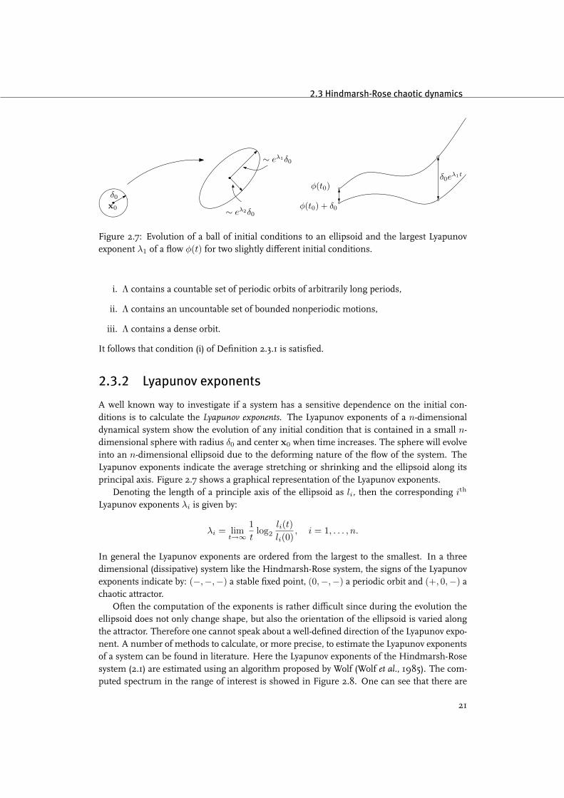
A well known way to investigate if a system has a sensitive dependence on the initial con-ditions is to calculate the Lyapunov exponents. The Lyapunov exponents of a n-dimensionaldynamical system show the evolution of any initial condition that is contained in a small n-dimensional sphere with radius δ0 and center x0 when time increases. The sphere will evolveinto an n-dimensional ellipsoid due to the deforming nature of the flow of the system. TheLyapunov exponents indicate the average stretching or shrinking and the ellipsoid along itsprincipal axis. Figure 2.7 shows a graphical representation of the Lyapunov exponents.
Denoting the length of a principle axis of the ellipsoid as li, then the corresponding ith
Lyapunov exponents λi is given by:
λi = limt→∞
1t
log2
li(t)li(0)
, i = 1, . . . , n.
In general the Lyapunov exponents are ordered from the largest to the smallest. In a threedimensional (dissipative) system like the Hindmarsh-Rose system, the signs of the Lyapunovexponents indicate by: (−,−,−) a stable fixed point, (0,−,−) a periodic orbit and (+, 0,−) achaotic attractor.
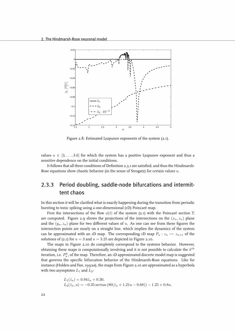
Often the computation of the exponents is rather difficult since during the evolution theellipsoid does not only change shape, but also the orientation of the ellipsoid is varied alongthe attractor. Therefore one cannot speak about a well-defined direction of the Lyapunov expo-nent. A number of methods to calculate, or more precise, to estimate the Lyapunov exponentsof a system can be found in literature. Here the Lyapunov exponents of the Hindmarsh-Rosesystem (2.1) are estimated using an algorithm proposed by Wolf (Wolf et al., 1985). The com-puted spectrum in the range of interest is showed in Figure 2.8. One can see that there are
21
2. The Hindmarsh-Rose neuronal model
1.5 2 2.5 3 3.5 4 4.5 5−0.14
−0.12
−0.1
−0.08
−0.06
−0.04
−0.02
0
0.02
u
λi[b
its
s]
λ1
λ2
λ3 · 10−2
Figure 2.8: Estimated Lyapunov exponents of the system (2.1).
values u ∈ [3, . . . , 3.6] for which the system has a positive Lyapunov exponent and thus asensitive dependence on the initial conditions.
It follows that all three conditions of Definition 2.3.1 are satisfied, and thus theHindmarsh-Rose equations show chaotic behavior (in the sense of Strogatz) for certain values u.
2.3.3 Period doubling, saddle-node bifurcations and intermit-tent chaos
In this section it will be clarified what is exactly happening during the transition from periodicbursting to tonic spiking using a one-dimensional (1D) Poincaré map.
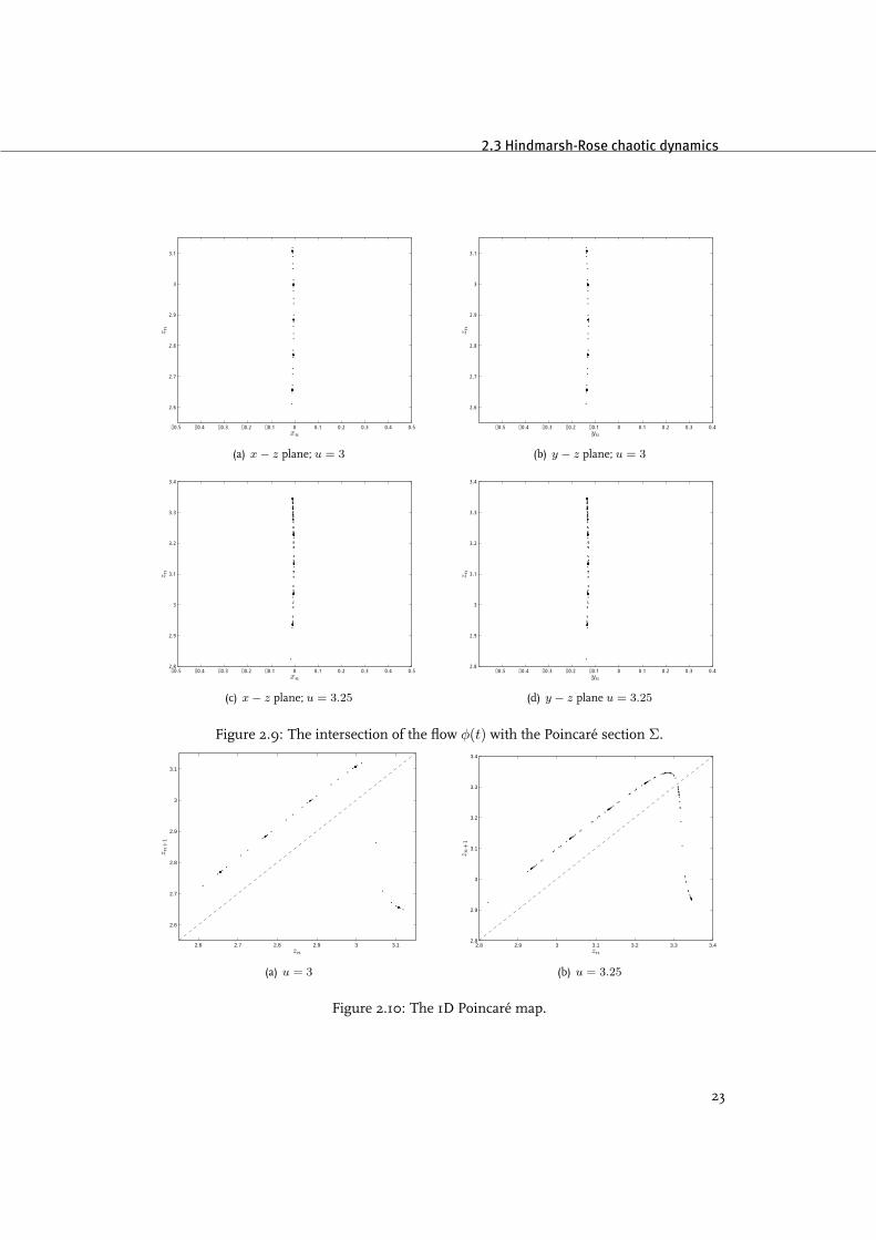
First the intersections of the flow φ(t) of the system (2.1) with the Poincaré section Σare computed. Figure 2.9 shows the projections of the intersections on the (xn, zn) planeand the (yn, zn) plane for two different values of u. As one can see from these figures theintersection points are nearly on a straight line, which implies the dynamics of the systemcan be approximated with an 1D map. The corresponding 1D map Pu : zn 7→ zn+1 of thesolutions of (2.1) for u = 3 and u = 3.25 are depicted in Figure 2.10.
The maps in Figure 2.10 do completely correspond to the systems behavior. However,obtaining these maps is computationally involving and it is not possible to calculate the kth
iteration, i.e. P ku , of the map. Therefore, an 1D approximated discrete model map is suggested
that governs the specific bifurcation behavior of the Hindmarsh-Rose equations. Like forinstance (Holden and Fan, 1992a), themaps from Figure 2.10 are approximated as a hyperbolawith two asymptotes L1 and L2:
L1(zn) = 0.94zn + 0.30,
L2(zn, u) = −0.35 arctan (80(zn + 1.21u− 0.68))− 1.25 + 0.8u.
22
2.3 Hindmarsh-Rose chaotic dynamics
−0.5 −0.4 −0.3 −0.2 −0.1 0 0.1 0.2 0.3 0.4 0.5
2.6
2.7
2.8
2.9
3
3.1
xn
z n
(a) x− z plane; u = 3
−0.5 −0.4 −0.3 −0.2 −0.1 0 0.1 0.2 0.3 0.4
2.6
2.7
2.8
2.9
3
3.1
yn
z n(b) y − z plane; u = 3
−0.5 −0.4 −0.3 −0.2 −0.1 0 0.1 0.2 0.3 0.4 0.52.8
2.9
3
3.1
3.2
3.3
3.4
xn
z n
(c) x− z plane; u = 3.25
−0.5 −0.4 −0.3 −0.2 −0.1 0 0.1 0.2 0.3 0.42.8
2.9
3
3.1
3.2
3.3
3.4
yn
z n
(d) y − z plane u = 3.25
Figure 2.9: The intersection of the flow φ(t) with the Poincaré section Σ.
2.6 2.7 2.8 2.9 3 3.1
2.6
2.7
2.8
2.9
3
3.1
zn
z n+
1
(a) u = 3
2.8 2.9 3 3.1 3.2 3.3 3.42.8
2.9
3
3.1
3.2
3.3
3.4
zn
z n+
1
(b) u = 3.25
Figure 2.10: The 1D Poincaré map.
23
2. The Hindmarsh-Rose neuronal model
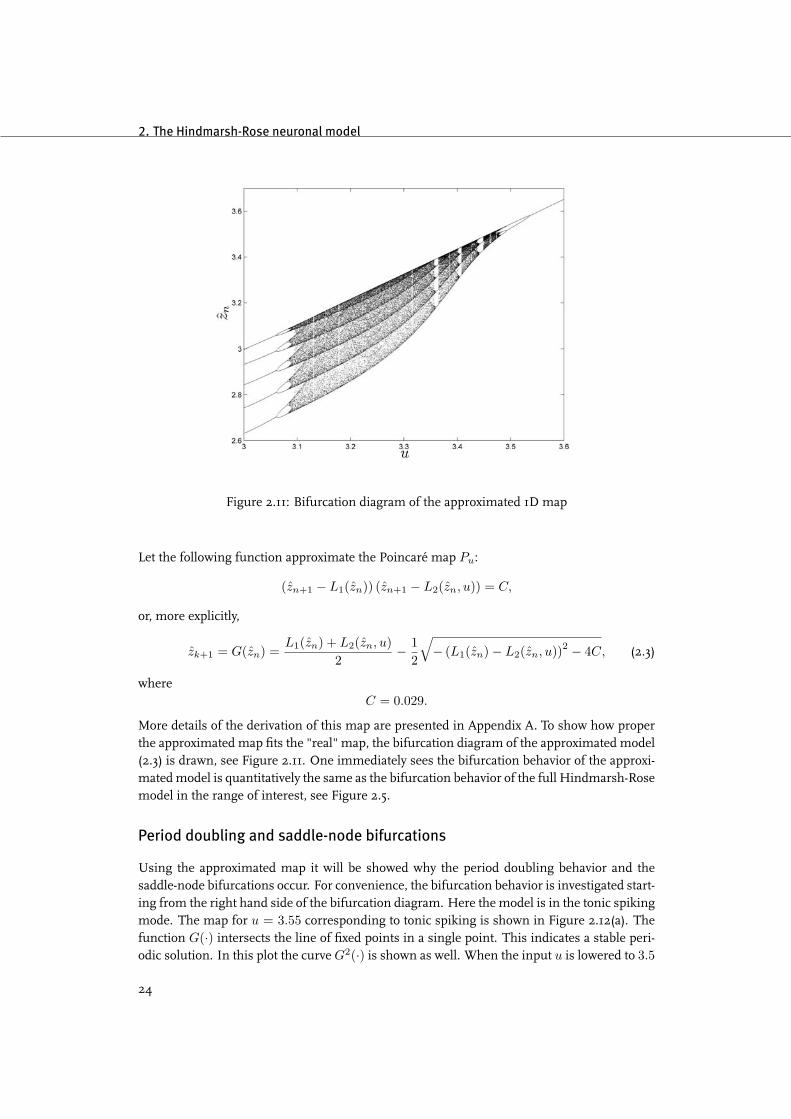
Figure 2.11: Bifurcation diagram of the approximated 1D map
Let the following function approximate the Poincaré map Pu:
(zn+1 − L1(zn)) (zn+1 − L2(zn, u)) = C,
or, more explicitly,
zk+1 = G(zn) =L1(zn) + L2(zn, u)
2− 1
2
√− (L1(zn)− L2(zn, u))2 − 4C, (2.3)
whereC = 0.029.
More details of the derivation of this map are presented in Appendix A. To show how properthe approximated map fits the "real" map, the bifurcation diagram of the approximated model(2.3) is drawn, see Figure 2.11. One immediately sees the bifurcation behavior of the approxi-matedmodel is quantitatively the same as the bifurcation behavior of the full Hindmarsh-Rosemodel in the range of interest, see Figure 2.5.
Period doubling and saddle-node bifurcations
Using the approximated map it will be showed why the period doubling behavior and thesaddle-node bifurcations occur. For convenience, the bifurcation behavior is investigated start-ing from the right hand side of the bifurcation diagram. Here the model is in the tonic spikingmode. The map for u = 3.55 corresponding to tonic spiking is shown in Figure 2.12(a). Thefunction G(·) intersects the line of fixed points in a single point. This indicates a stable peri-odic solution. In this plot the curve G2(·) is shown as well. When the input u is lowered to 3.5
24
2.4 Summary
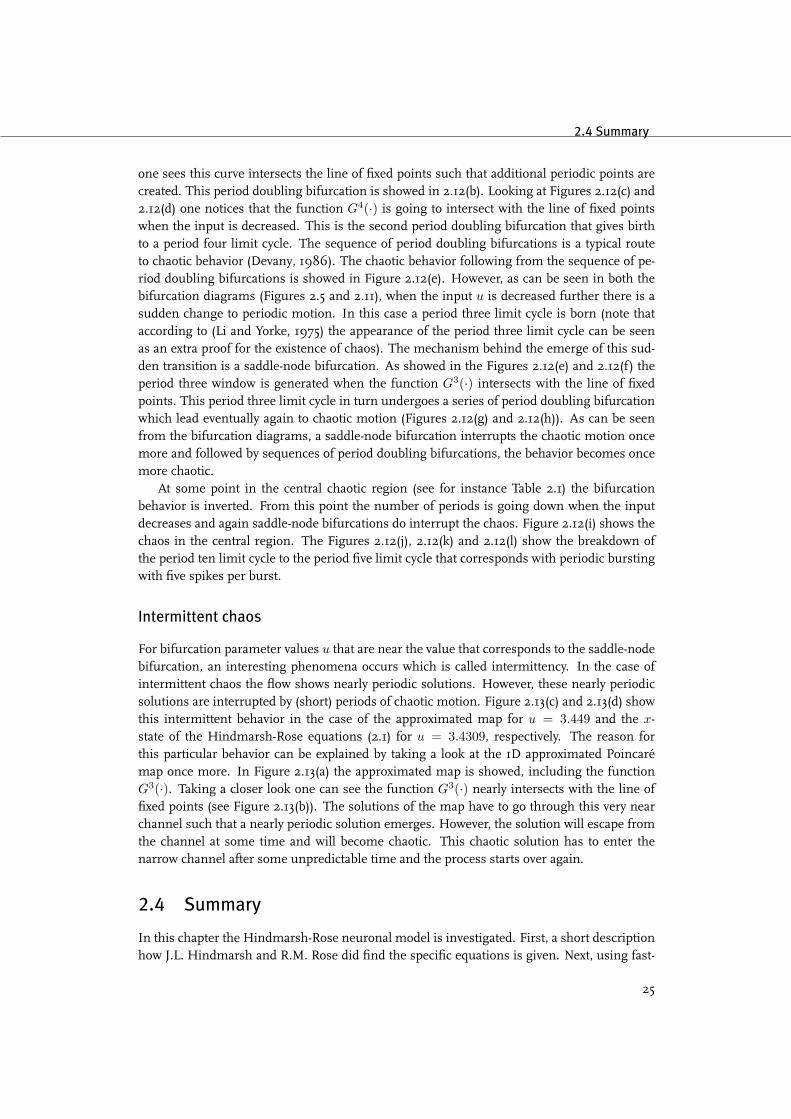
one sees this curve intersects the line of fixed points such that additional periodic points arecreated. This period doubling bifurcation is showed in 2.12(b). Looking at Figures 2.12(c) and2.12(d) one notices that the function G4(·) is going to intersect with the line of fixed pointswhen the input is decreased. This is the second period doubling bifurcation that gives birthto a period four limit cycle. The sequence of period doubling bifurcations is a typical routeto chaotic behavior (Devany, 1986). The chaotic behavior following from the sequence of pe-riod doubling bifurcations is showed in Figure 2.12(e). However, as can be seen in both thebifurcation diagrams (Figures 2.5 and 2.11), when the input u is decreased further there is asudden change to periodic motion. In this case a period three limit cycle is born (note thataccording to (Li and Yorke, 1975) the appearance of the period three limit cycle can be seenas an extra proof for the existence of chaos). The mechanism behind the emerge of this sud-den transition is a saddle-node bifurcation. As showed in the Figures 2.12(e) and 2.12(f) theperiod three window is generated when the function G3(·) intersects with the line of fixedpoints. This period three limit cycle in turn undergoes a series of period doubling bifurcationwhich lead eventually again to chaotic motion (Figures 2.12(g) and 2.12(h)). As can be seenfrom the bifurcation diagrams, a saddle-node bifurcation interrupts the chaotic motion oncemore and followed by sequences of period doubling bifurcations, the behavior becomes oncemore chaotic.
At some point in the central chaotic region (see for instance Table 2.1) the bifurcationbehavior is inverted. From this point the number of periods is going down when the inputdecreases and again saddle-node bifurcations do interrupt the chaos. Figure 2.12(i) shows thechaos in the central region. The Figures 2.12(j), 2.12(k) and 2.12(l) show the breakdown ofthe period ten limit cycle to the period five limit cycle that corresponds with periodic burstingwith five spikes per burst.
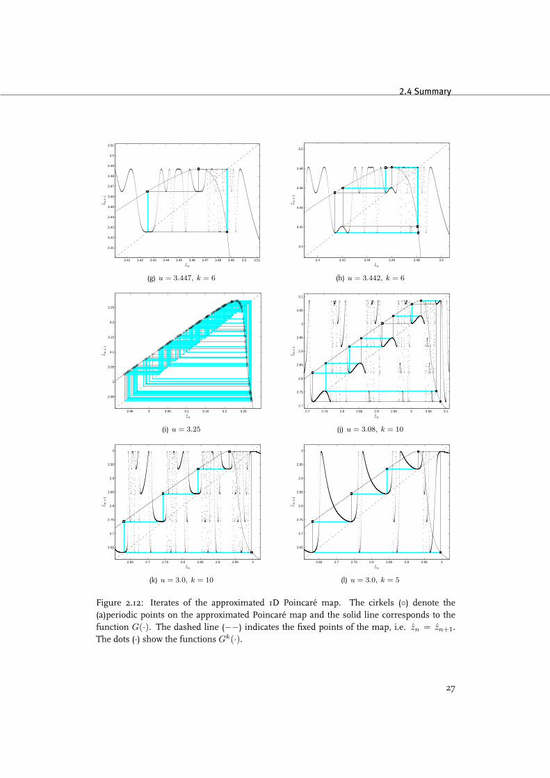
Intermittent chaos
For bifurcation parameter values u that are near the value that corresponds to the saddle-nodebifurcation, an interesting phenomena occurs which is called intermittency. In the case ofintermittent chaos the flow shows nearly periodic solutions. However, these nearly periodicsolutions are interrupted by (short) periods of chaotic motion. Figure 2.13(c) and 2.13(d) showthis intermittent behavior in the case of the approximated map for u = 3.449 and the x-state of the Hindmarsh-Rose equations (2.1) for u = 3.4309, respectively. The reason forthis particular behavior can be explained by taking a look at the 1D approximated Poincarémap once more. In Figure 2.13(a) the approximated map is showed, including the functionG3(·). Taking a closer look one can see the function G3(·) nearly intersects with the line offixed points (see Figure 2.13(b)). The solutions of the map have to go through this very nearchannel such that a nearly periodic solution emerges. However, the solution will escape fromthe channel at some time and will become chaotic. This chaotic solution has to enter thenarrow channel after some unpredictable time and the process starts over again.
2.4 Summary
In this chapter the Hindmarsh-Rose neuronal model is investigated. First, a short descriptionhow J.L. Hindmarsh and R.M. Rose did find the specific equations is given. Next, using fast-
25

2. The Hindmarsh-Rose neuronal model
3.575 3.58 3.585 3.59 3.595 3.6 3.605 3.61 3.615 3.62
3.575
3.58
3.585
3.59
3.595
3.6
3.605
3.61
3.615
3.62
zn
z n+
1
(a) u = 3.55, k = 2
3.51 3.52 3.53 3.54 3.55 3.56
3.51
3.52
3.53
3.54
3.55
3.56
zn
z n+
1(b) u = 3.5, k = 2
3.51 3.52 3.53 3.54 3.55 3.56
3.51
3.52
3.53
3.54
3.55
3.56
zn
z n+
1
(c) u = 3.5, k = 4
3.49 3.5 3.51 3.52 3.53 3.54 3.55
3.49
3.5
3.51
3.52
3.53
3.54
3.55
zn
z n+
1
(d) u = 3.49, k = 4
3.43 3.44 3.45 3.46 3.47 3.48 3.49 3.5 3.51 3.523.43
3.44
3.45
3.46
3.47
3.48
3.49
3.5
3.51
3.52
zn
z n+
1
(e) u = 3.46, k = 3
3.41 3.42 3.43 3.44 3.45 3.46 3.47 3.48 3.49 3.5 3.51
3.41
3.42
3.43
3.44
3.45
3.46
3.47
3.48
3.49
3.5
3.51
zn
z n+
1
(f) u = 3.447, k = 3
Caption on the next page.
26
2.4 Summary
3.41 3.42 3.43 3.44 3.45 3.46 3.47 3.48 3.49 3.5 3.51
3.41
3.42
3.43
3.44
3.45
3.46
3.47
3.48
3.49
3.5
3.51
zn
z n+
1
(g) u = 3.447, k = 6
3.4 3.42 3.44 3.46 3.48 3.5
3.4
3.42
3.44
3.46
3.48
3.5
zn
z n+
1
(h) u = 3.442, k = 6
2.95 3 3.05 3.1 3.15 3.2 3.25
2.95
3
3.05
3.1
3.15
3.2
3.25
zn
z n+
1
(i) u = 3.25
2.7 2.75 2.8 2.85 2.9 2.95 3 3.05 3.1
2.7
2.75
2.8
2.85
2.9
2.95
3
3.05
3.1
zn
z n+
1
(j) u = 3.08, k = 10
2.65 2.7 2.75 2.8 2.85 2.9 2.95 3
2.65
2.7
2.75
2.8
2.85
2.9
2.95
3
zn
z n+
1
(k) u = 3.0, k = 10
2.65 2.7 2.75 2.8 2.85 2.9 2.95 3
2.65
2.7
2.75
2.8
2.85
2.9
2.95
3
zn
z n+
1
(l) u = 3.0, k = 5
Figure 2.12: Iterates of the approximated 1D Poincaré map. The cirkels () denote the(a)periodic points on the approximated Poincaré map and the solid line corresponds to thefunction G(·). The dashed line (−−) indicates the fixed points of the map, i.e. zn = zn+1.The dots (·) show the functions Gk(·).
27
2. The Hindmarsh-Rose neuronal model
3.41 3.42 3.43 3.44 3.45 3.46 3.47 3.48 3.49 3.5 3.51
3.41
3.42
3.43
3.44
3.45
3.46
3.47
3.48
3.49
3.5
3.51
zn
zn+
1
(a)
3.4684 3.4686 3.4688 3.469 3.4692 3.4694 3.4696 3.4698 3.473.4684
3.4686
3.4688
3.469
3.4692
3.4694
3.4696
3.4698
3.47
zn
zn+
1
(b)
0 50 100 150 200 250 3003.43
3.44
3.45
3.46
3.47
3.48
3.49
3.5
zn
] iterates
(c)
0 0.2 0.4 0.6 0.8 1 1.2 1.4 1.6 1.8 2−2.5
−2
−1.5
−1
−0.5
0
0.5
1
x[V
]
time [s]
(d)
Figure 2.13: Intermittent chaos near the period three saddle-node bifurcation
slow analysis the general generation of the bursting and/or spiking behavior is explained.The fast subsystem is responsible for the existence of a limit motion corresponding to thespikes with a firing frequency that is dependent on the given input, while the slow systemacts as perturbation on this input and thus changes the firing frequency. As showed in thebifurcation diagram, for a certain range of inputs the system behaves chaotically. This chaoscan be explained by the presence of horseshoe like dynamics and a sensible dependence oninitial conditions. Finally the specific bifurcation behavior of the model is explained using anapproximated 1D map.
28
Chapter 3
Realization and identification of theelectromechanical neuron
In this chapter the realization of the electromechanical Hindmarsh-Rose circuits will be pre-sented. Several experiments will show the performance of the electromechanical neuron.Given that the trajectories that are generated by the realization will possibly differ from thoseof the model, the circuits will be identified such that these differences can be quantified.
3.1 Realization
There are several publications on the realization on electronic neurons, see for instance (Lewis,1968), (Roy, 1972) and (Linares-Barranco et al., 1991). Electronic implementations of theHindmarsh-Rose model in particular have been published by (Merlat et al., 1996) and (Leeet al., 2004). The electromechanical neuron as developed during this project is based on thework described in the latter.
A single electromechanical Hindmarsh-Rose neuron consists basically of three integrator cir-cuits, which integrate the three states of the Hindmarsh-Rose model, and a multiplier circuitthat generates the squared and cubic terms that are present in the equations.
Every state of the Hindmarsh-Rose model is modeled as a voltage, since most data ac-quisition devices, oscilloscopes or SigLab for instance, measure voltages instead of currents.In addition, the input for the electromechanical neuron is chosen to be applied as a voltagewhereas the input of the model is actually a current. The main reason for this choice is thatit is more convenient (and more safe) to supply a voltage rather then a current. The valuesof the resistors and capacitors are chosen such that they match the parameters of the modelas mentioned in the previous chapter. Note this particular parameter set is chosen such thatpossible saturation of the operational amplifiers is avoided.
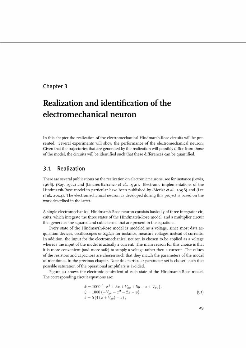
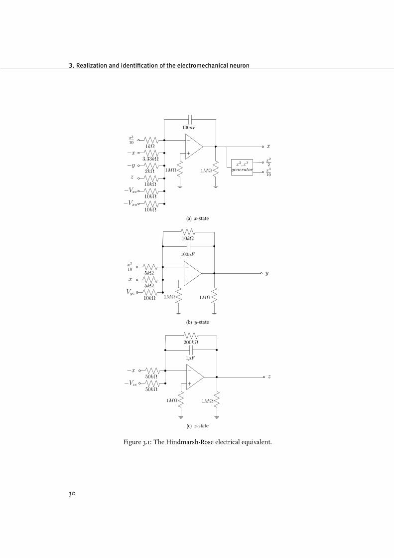
Figure 3.1 shows the electronic equivalent of each state of the Hindmarsh-Rose model.The corresponding circuit equations are:
x = 1000(−x3 + 3x + Vxc + 5y − z + Vxu
),
y = 1000(−Vyc − x2 − 2x− y
),
z = 5 (4 (x + Vzc)− z) ,
(3.1)
29
3. Realization and identification of the electromechanical neuron
x
x2
2x3
10
x2, x3
1MΩ 1MΩ generator
100nF
1kΩ
3.33kΩ
2kΩ
10kΩ
10kΩ
10kΩ
+
−x3
10
−x
−y
z
−Vxc
−Vxu
(a) x-state
y
1MΩ 1MΩ
100nF
5kΩ
5kΩ
10kΩ
+
−x2
10
x
Vyc
10kΩ
(b) y-state
z
1MΩ 1MΩ
1µF
50kΩ
50kΩ+
−−x
−Vzc
200kΩ
(c) z-state
Figure 3.1: The Hindmarsh-Rose electrical equivalent.
30
3.2 Experiments
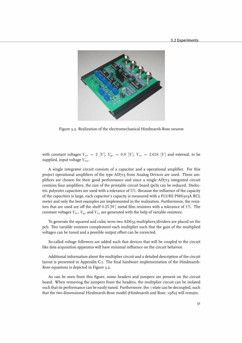
Figure 3.2: Realization of the electromechanical Hindmarsh-Rose neuron
with constant voltages Vxc = 2 [V ], Vyc = 0.8 [V ], Vzc = 2.618 [V ] and external, to besupplied, input voltage Vxu.
A single integrator circuit consists of a capacitor and a operational amplifier. For thisproject operational amplifiers of the type AD713 from Analog Devices are used. These am-plifiers are chosen for their good performance and since a single AD713 integrated circuitcontains four amplifiers, the size of the printable circuit board (pcb) can be reduced. Dielec-tric polyester capacitors are used with a tolerance of 5%. Because the influence of the capacityof the capacitors is large, each capacitor’s capacity is measured with a FLUKE PM6303A RCLmeter and only the best examples are implemented in the realization. Furthermore, the resis-tors that are used are off the shelf 0.25 [W ] metal film resistors with a tolerance of 1%. Theconstant voltages Vxc, Vyc and Vzc are generated with the help of variable resistors.
To generate the squared and cubic term two AD633 multipliers/dividers are placed on thepcb. Two variable resistors complement each multiplier such that the gain of the multipliedvoltages can be tuned and a possible output offset can be corrected.
So-called voltage followers are added such that devices that will be coupled to the circuitlike data acquisition apparatus will have minimal influence on the circuit behavior.
Additional information about the multiplier circuit and a detailed description of the circuitlayout is presented in Appendix C.1. The final hardware implementation of the Hindmarsh-Rose equations is depicted in Figure 3.2.
As can be seen from this figure, some headers and jumpers are present on the circuitboard. When removing the jumpers from the headers, the multiplier circuit can be isolatedsuch that its performance can be easily tuned. Furthermore, the z-state can be decoupled, suchthat the two dimensional Hindmarsh-Rose model (Hindmarsh and Rose, 1982) will remain.
31
3. Realization and identification of the electromechanical neuron
3.2 Experiments
The electronic realization of the Hindmarsh-Rose neuron will be compared to the nominalbehavior of the system as shown in the previous chapter. The measured data is obtained withthe help of a SigLab data acquisition device. The experiments are performed with a constantinput voltage. In Figure 3.3 some responses of the electromechanical neuron are shown asfunction of a constant input voltage. On the left the time signals of the states are showedfor various inputs and the corresponding attractors are given in the figure on the right. InFigure 3.3(a) the circuit operates in the period two bursting mode when an input of u = 2 [V ]is applied. This is exactly the mode that is expected as can be seen in Figure 2.2(a) and thebifurcation diagram in Figure 2.5 in the previous chapter. When the input voltage is increasedto u = 3.25 [V ], the circuit produces chaotic burst. This experimental data is presented inFigure 3.3(b) and, again, this result confirms the simulations. Figure 3.3(c) shows the stablelimit cycle with u = 5 [V ] that corresponds with the continuous spiking mode. Once more,the responses of the circuit confirm the simulated responses. In Appendix E.1 responses ofthe electromechanical Hindmarsh-Rose neuron are presented for various inputs.
3.3 Identification
Although the values of the capacitors and resistors are measured a priori and only the bestexamples are included in the circuits, there are, as shown at the end of this section, somedifferences between the simulated outputs and the measured outputs. In addition, the inter-nal circuit board resistances are unknown and the used integrated circuits might not be fullyaccurate. In order to quantify the differences between the responses of the model and thecircuits identification of the systems is performed.
In order to reduce the number of parameters that has to be estimated at once the problemof identification is split up in identification of the fast subsystem and identification of the slowsubsystem. First, the parameters of the slow subsystem will be estimated.
3.3.1 Identification of the slow subsystem
The slow subsystem is an state affine linear system that is given by the differential equation
z = rsx− rsx0 − rz. (3.2)
In this equation x is regarded as the input function, z is the state and r, s, x0 are the pa-rameters to be estimated. Several fast and well established parameter estimation methods forlinear systems are available in literature, see for instance (Ljung, 1999). However, to applythose procedures one has to cancel the constant term rsx0 in (3.2).
Consider two series of measurements, z1 and z2, recorded with the input signals x = x1
and x = x2, respectively. At least one signal zi(t), i = 1, 2, should have an transient. Let thecorresponding systems be written as
z1 = rsx1 − rsx0 − rz1,
z2 = rsx2 − rsx0 − rz2.
32

3.3 Identification
0 0.2 0.4 0.6 0.8 1
−2
−1
0
1
x[V
]
0 0.2 0.4 0.6 0.8 1
−2
−1
0
y[V
]
0 0.2 0.4 0.6 0.8 1
1.8
2
2.2
time [s]
z[V
]
−2−1.5
−1−0.5
0
−2
−1
0
1.8
1.9
2
2.1
y [V ]x [V ]
z[V
]
(a)
0 0.2 0.4 0.6 0.8 1
−2
−1
0
1
x[V
]
0 0.2 0.4 0.6 0.8 1
−1.5−1
−0.50
y[V
]
0 0.2 0.4 0.6 0.8 1
3
3.5
time [s]
z[V
]
−1.5−1
−0.50
−2
−1
0
2.9
3
3.1
3.2
3.3
3.4
y [V ]x [V ]
z[V
]
(b)
0 0.05 0.1 0.15 0.2−2
−1
0
1
x[V
]
0 0.05 0.1 0.15 0.2−1.5
−1
−0.5
0
y[V
]
0 0.05 0.1 0.15 0.24.7
4.8
4.9
time [s]
z[V
]
−1
−0.5
0
−1.5−1
−0.50
0.5
4.76
4.77
4.78
4.79
4.8
4.81
y [V ]x [V ]
z[V
]
(c)
Figure 3.3: Responses of the electromechanical Hindmarsh-Rose neuron.
33
3. Realization and identification of the electromechanical neuron
Denote z = z1 − z2 as new output, x = x1 − x2 as new input, then the following holds:
˙z = rsx− rz. (3.3)
The system (3.3) is the desired (first order) linear system. The general approach for estimationof parameters of linear systems is to use prediction error identification methods (PEM). First,denote the estimated output of the system (3.3) by ˆz(t, θz), where θz ∈ R2 is an vector con-taining the estimates of the parameters r and s. In advance, the prediction error is givenby
ε(t, θz) = z(t)− ˆz(t, θz).
Consider the following norm
VN (θz, ZN ) =
1N
N∑t=1
`(ε(t, θ)), (3.4)
where ` is a class-K function and ZN = [z(1), x(1), z(2), x(2), . . . , z(N), x(N)] is the (dis-crete) set of data that is, in this case, sampled with a frequency of 12.8 [kHz]. The problem offinding proper estimations of the parameters θz is now defined as minimization of (3.4), i.e.
θz = θz(ZN ) = arg minθz∈R2
VN (θz, ZN ),
where arg min denotes the minimization with respect to the argument of the function. Al-gorithms to solve this optimization problem can be found in, for instance, (Ljung, 1999).Here, the Matlab System Identification Toolbox is used to determine the estimates r and s inan efficient way. Given the estimations of the parameters r and s, an estimated value of theparameter x0 can be calculated with the following equation:
x0 =1s(zi(t)− z′(t)),
where i = 1 ∨ 2 and z′(t) is the solution defined by the system
z′ = rsxi − rz′, z′(0) = 0,
after some transient behavior.
3.3.2 Identification of the fast subsystem
The fast subsystem is a nonlinear system and thus different identification techniques are re-quired. A popular and well established method to estimate the parameters of continuous-timenonlinear systems from measurements is to use the continuous-discrete augmented extendedKalman filter. The filter minimizes the variance of the estimated state as function of the mea-sured data. The term extended refers to the fact that the considered system has nonlinear dy-namics. The filter deals with the nonlinearities by means of first order Taylor approximationsalong the estimated trajectories. The filter is continuous-discrete since the model is continu-ous, whereas the measured data is of the discrete type. Finally, augmentedmeans that the statevector is extended with the values of the parameters, i.e. η(t) = x(t) ⊕ θ, where θ ∈ Rd is avector containing the, assumed constant, parameters values.
34
3.3 Identification
The continuous-discrete augmented extended Kalman filter
The continuous-discrete augmented extended Kalman filter as described in (Gelb, 1996) isimplemented. This filter algorithm starts with the continuous system model and the discretemeasurement model:
η = f(η(t), t) + w(t), w(t) ∼ N(0,Q(t)),zk = hk(η(tk)) + vk, v ∼ N(0,Rk),
where states η ∈ Rn, zk ∈ Rn, functions f : Rn × R+ → Rn, hk : Rn → Rn and the processand measurement noise w : R+ → Rn and vk ∈ Rn, respectively. Both w(t) and vk areassumed to be zero mean gaussian noises with corresponding covariance matrices Q(t) andRk. Since the measurements are discrete and thus not available at any instance of time, it isnecessary to calculate the propagation of the estimated extended state η(t) and the estimationerror covariance matrix P(t). Suppose the measurement at time tk is just processed and thusthe estimate η(tk) is known. Between tk and tk+1 there is no information available from themeasurements. At this interval the state will propagate according to
˙η(t) = f(η(t), t).
Similarly the propagation of the estimation error covariance matrix can be determined bysolving
P(t) = F(η(t), t)P(t) + P(t)FT (η(t), t) + Q(t),
where the Jacobian F(η(t), t) is defined as
F(η(t), t) =∂f(η(t), t)
∂η(t)
∣∣∣∣η(t)=η(t)
.
If a new measurement is available the state and the estimation error covariance matrix willbe updated. Denote the a priori solutions at time tk by ηk(−) and Pk(−). At the time ameasurement is taken updated estimations of the state and the estimation error covariancematrix, i.e. ηk(+) and Pk(+), are obtained from the equations
ηk(+) = ηk(−) + Kk [zk − hk(ηk(−))] ,
Pk(+) = [I−KkHk(ηk(−))]Pk(−),
where the Kalman gainmatrix Kk is given by
Kk = Pk(−)HT (ηk(−))[Hk(ηk(−))Pk(−)HT
k (ηk(−)) + Rk
]−1, (3.5)
and the Jacobian Hk(η(−)) is defined as
Hk(η(−)) =∂h(η(tk))
∂η(tk)
∣∣∣∣η(tk)=ηk(−)
.
A schematic representation of the continuous-discrete augmented extended Kalman filter isdepicted in Figure 3.4.
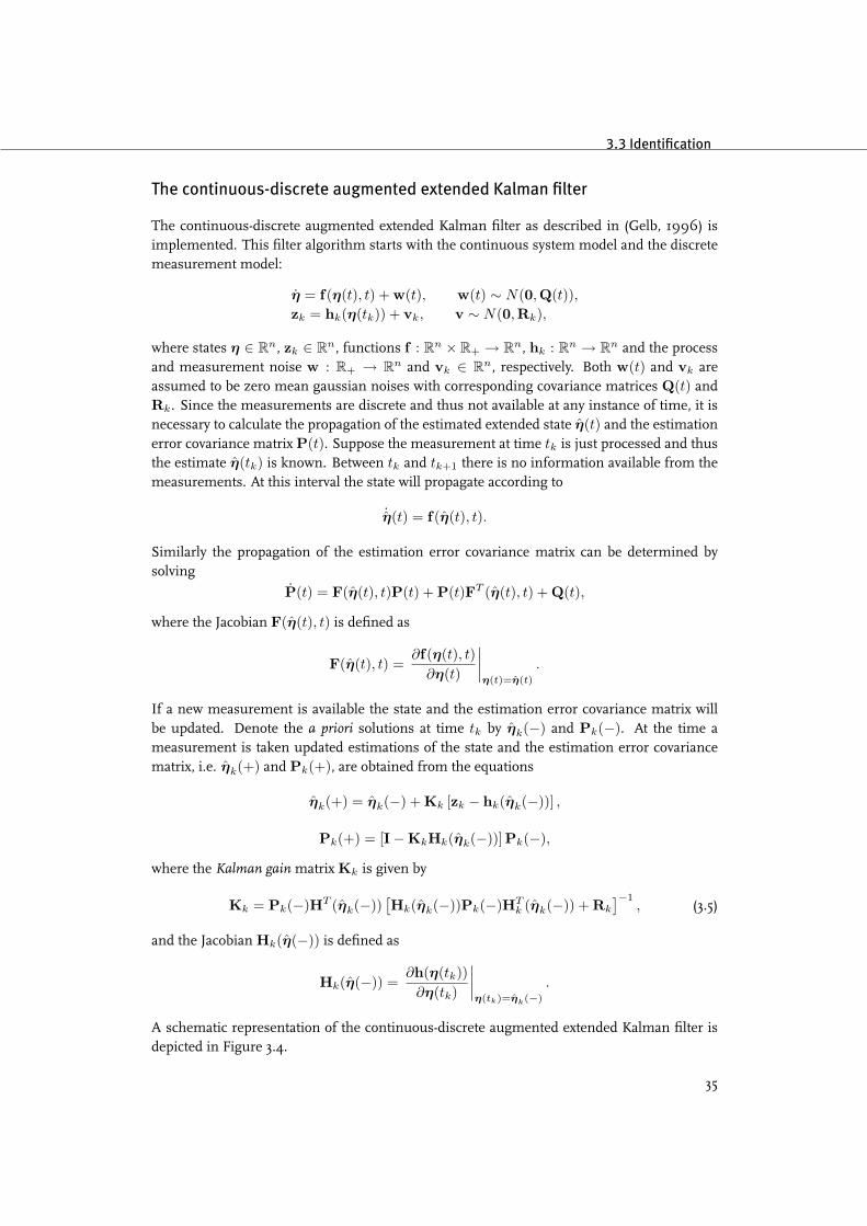
35
3. Realization and identification of the electromechanical neuron
Update Propagation
Initialization
Figure 3.4: The continuous-discrete extended Kalman filter scheme.
Filter initialization
Before the filter algorithm can be used to estimate the parameters, some starting condi-tions have to be determined. At first initial values have to be assigned to the extended stateη = [x, y, z, a, ϕ1, ϕ2, gy, gz, α, c, d, ϕ3, β]T ∈ R13 and the error estimation covariancematrix P.
The initial values of x, y and z are chosen to be equal to the correspondingmeasured statesat t = t0, i.e. z0. Furthermore, the initial estimates of the parameter values are set equal tothe nominal parameter values. The initial error estimation covariance matrix P0 contains thedifferences of the initial estimations η(t0) with respect to the initial vector η0. Assuming thatall states are mutually independent , the matrix P becomes diagonal. This diagonal can bedivided into two parts. The first part, denoted by Px,0, contains the initial error with respectto the measured states and the corresponding estimated states, and the second part, Pθ,0,indicates the initial amount of uncertainty in the parameter estimations. Since the initialvalues of x, y and z are measured directly, Px,0 is chosen small, i.e. Px,0 = 10−6 · I3.The initial values in Pθ,0 are specified by the tolerances of the used electrical components.As mentioned before, the capacitors have a tolerance of 5% and the tolerances of the usedresistors are 1%. Given that each parameter θi can be represented as a combination of acapacitor and a resistor, i.e. θi = 1
CiRi, it is easy to verify that the maximum difference
between the nominal value and the value to be estimated is within 7%. Therefore Pθ =0.072 · I10.
It is assumed that the uncertainties in the model equations are independent. It is alsoassumed that the measurements of the states, that are corrupted with noise, are uncorrelated.Therefore, the covariance matrices Q(t) and Rk are chosen as diagonal matrices. In advance,it is assumed that the covariances are time-independent such that both Q(t) and Rk are con-stant matrices.
The signals of the Hindmarsh-Rose circuit are recorded using a SigLab data acquisitiondevice with a 16-bit resolution over a range of ±5 [V ]. Each state can thus be measured withan accuracy of 10
2·216 [V ] ≈ 1 · 10−4 [V ]. According the the specifications of the SigLab othersources of noise are negligibly small. The parameter values can not be directly measured.However, measurement noise is assigned to the corresponding diagonal entries of the matrixRk. This is necessary in order to avoid singularities in the computation of the Kalman gain(3.5), i.e. Rk should be positive definite. The matrixRk is now chosen to beRk = 1·10−4 ·I13.
36
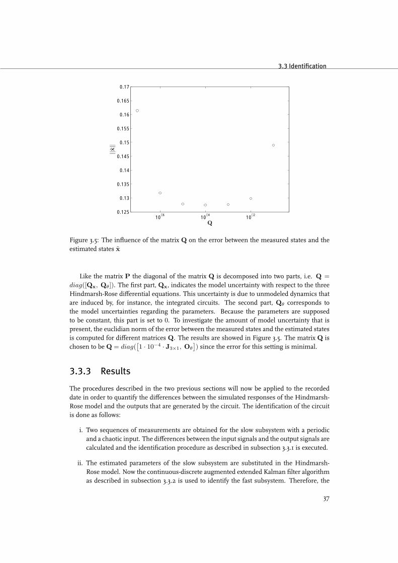
3.3 Identification
10−6
10−4
10−2
0.125
0.13
0.135
0.14
0.145
0.15
0.155
0.16
0.165
0.17
Q
||x||
Figure 3.5: The influence of the matrix Q on the error between the measured states and theestimated states x
Like the matrix P the diagonal of the matrix Q is decomposed into two parts, i.e. Q =diag([Qx, Qθ]). The first part, Qx, indicates the model uncertainty with respect to the threeHindmarsh-Rose differential equations. This uncertainty is due to unmodeled dynamics thatare induced by, for instance, the integrated circuits. The second part, Qθ corresponds tothe model uncertainties regarding the parameters. Because the parameters are supposedto be constant, this part is set to 0. To investigate the amount of model uncertainty that ispresent, the euclidian norm of the error between the measured states and the estimated statesis computed for different matrices Q. The results are showed in Figure 3.5. The matrix Q ischosen to be Q = diag(
[1 · 10−4 · J3×1, Oθ
]) since the error for this setting is minimal.
3.3.3 Results
The procedures described in the two previous sections will now be applied to the recordeddate in order to quantify the differences between the simulated responses of the Hindmarsh-Rose model and the outputs that are generated by the circuit. The identification of the circuitis done as follows:
i. Two sequences of measurements are obtained for the slow subsystem with a periodicand a chaotic input. The differences between the input signals and the output signals arecalculated and the identification procedure as described in subsection 3.3.1 is executed.
ii. The estimated parameters of the slow subsystem are substituted in the Hindmarsh-Rose model. Now the continuous-discrete augmented extended Kalman filter algorithmas described in subsection 3.3.2 is used to identify the fast subsystem. Therefore, the
37
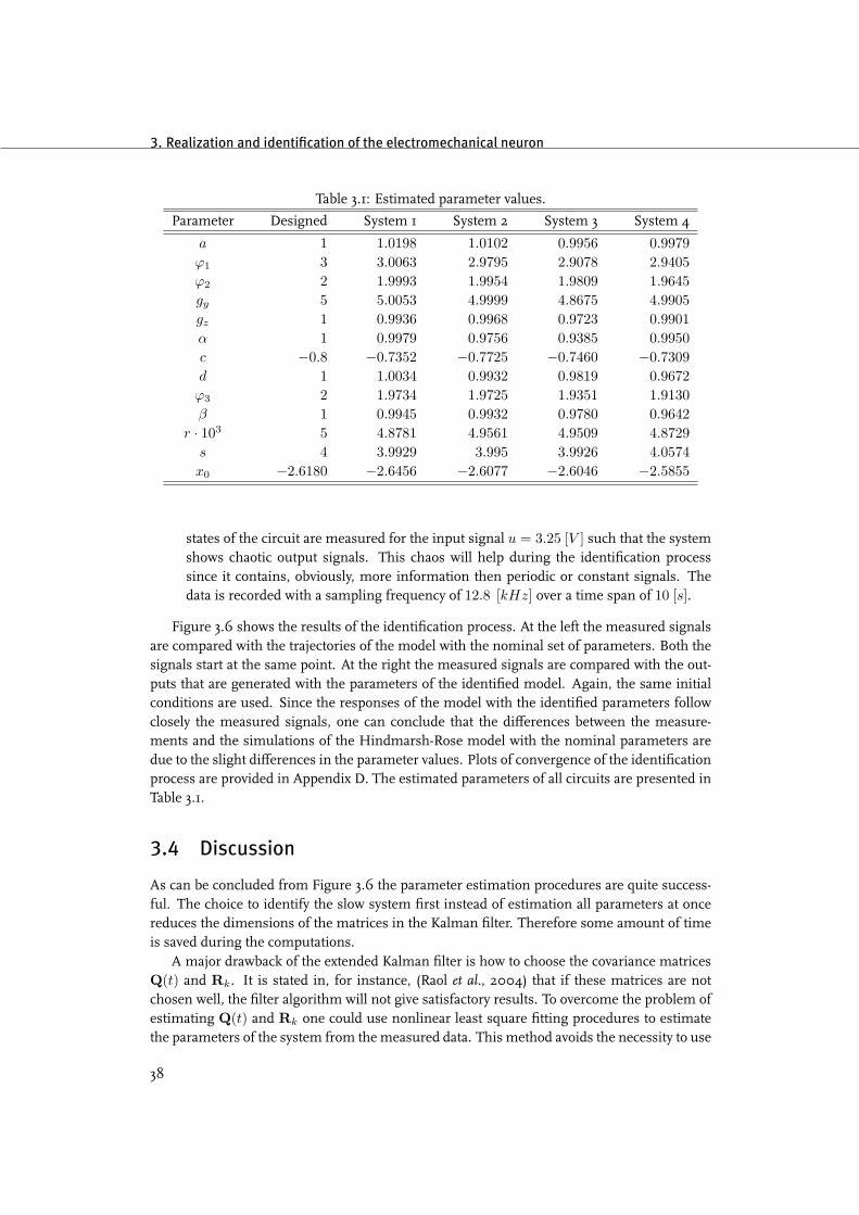
3. Realization and identification of the electromechanical neuron
Table 3.1: Estimated parameter values.
Parameter Designed System 1 System 2 System 3 System 4
a 1 1.0198 1.0102 0.9956 0.9979ϕ1 3 3.0063 2.9795 2.9078 2.9405ϕ2 2 1.9993 1.9954 1.9809 1.9645gy 5 5.0053 4.9999 4.8675 4.9905gz 1 0.9936 0.9968 0.9723 0.9901α 1 0.9979 0.9756 0.9385 0.9950c −0.8 −0.7352 −0.7725 −0.7460 −0.7309d 1 1.0034 0.9932 0.9819 0.9672ϕ3 2 1.9734 1.9725 1.9351 1.9130β 1 0.9945 0.9932 0.9780 0.9642
r · 103 5 4.8781 4.9561 4.9509 4.8729s 4 3.9929 3.995 3.9926 4.0574x0 −2.6180 −2.6456 −2.6077 −2.6046 −2.5855
states of the circuit are measured for the input signal u = 3.25 [V ] such that the systemshows chaotic output signals. This chaos will help during the identification processsince it contains, obviously, more information then periodic or constant signals. Thedata is recorded with a sampling frequency of 12.8 [kHz] over a time span of 10 [s].
Figure 3.6 shows the results of the identification process. At the left the measured signalsare compared with the trajectories of the model with the nominal set of parameters. Both thesignals start at the same point. At the right the measured signals are compared with the out-puts that are generated with the parameters of the identified model. Again, the same initialconditions are used. Since the responses of the model with the identified parameters followclosely the measured signals, one can conclude that the differences between the measure-ments and the simulations of the Hindmarsh-Rose model with the nominal parameters aredue to the slight differences in the parameter values. Plots of convergence of the identificationprocess are provided in Appendix D. The estimated parameters of all circuits are presented inTable 3.1.
3.4 Discussion
As can be concluded from Figure 3.6 the parameter estimation procedures are quite success-ful. The choice to identify the slow system first instead of estimation all parameters at oncereduces the dimensions of the matrices in the Kalman filter. Therefore some amount of timeis saved during the computations.
A major drawback of the extended Kalman filter is how to choose the covariance matricesQ(t) and Rk. It is stated in, for instance, (Raol et al., 2004) that if these matrices are notchosen well, the filter algorithm will not give satisfactory results. To overcome the problem ofestimating Q(t) and Rk one could use nonlinear least square fitting procedures to estimatethe parameters of the system from themeasured data. This method avoids the necessity to use
38

3.4 Discussion
−3−2
−10
1
−3
−2
−1
0
11.6
1.8
2
2.2
2.4
2.6
y [V ]x [V ]
z[V
]
OriginalExperiment
−3−2
−10
1
−3
−2
−1
0
11.6
1.8
2
2.2
2.4
2.6
y [V ]x [V ]
z[V
]
IdentifiedExperiment
(a)
−2−1.5
−1−0.5
00.5
−3
−2
−1
0
12.8
3
3.2
3.4
3.6
3.8
y [V ]x [V ]
z[V
]
OriginalExperiment
−2−1.5
−1−0.5
00.5
−3
−2
−1
0
12.8
3
3.2
3.4
3.6
y [V ]x [V ]
z[V
]
IdentifiedExperiment
(b)
−1.5−1
−0.50
0.5
−2
−1
0
14.7
4.75
4.8
4.85
4.9
4.95
y [V ]x [V ]
z[V
]
OriginalExperiment
−1.5−1
−0.50
0.5
−2
−1
0
14.82
4.84
4.86
4.88
4.9
4.92
y [V ]x [V ]
z[V
]
IdentifiedExperiment
(c)
Figure 3.6: Responses of the original model compared to the measurement, and responses ofthe identified model compared to the measurements. The constant inputs that are used are:3.6(a) u = 2 [V ], 3.6(b) u = 3.25 [V ] and 3.6(c) u = 5 [V ].
39

3. Realization and identification of the electromechanical neuron
the stochastic matrices Q(t) and Rk. However, algorithms to solve the least square problemfor the relatively large set of data that is used are, in general, not very efficient (Bertsekas,1996).
Here the Kalman filter is successfully implemented and, as can be seen in Figure 3.6, theresults are satisfactory.
3.5 Summary
In this chapter the realization of the electromechanical Hindmarsh-Rose neuron is discussed.Experiments with the circuits are performed and these results show quantitatively the samebehavior as observed in the simulations. The identification of the circuit shows that the dif-ferences between the model and the experimental setup can be explained by small differencesin the parameters.
40
Chapter 4
Synchronization of Hindmarsh-Roseneurons: General theory
This chapter focusses on the synchronization of an array of diffusively coupled Hindmarsh-Rose neurons, that is all systems aremutually coupled through linear output coupling (Pogrom-sky and Nijmeijer, 2001). First a theoretical framework for the design of synchronizing sys-tems (Pogromsky, 1998) is explained. This framework uses the concepts of semi-passive sys-tems and convergent systems to derive sufficient conditions for the existence of (global) syn-chronization manifolds, including manifolds corresponding to partial synchronization. Thetheory is applied to the Hindmarsh-Rose systems and it will be shown that the Hindmarsh-Rose systems can exhibit synchronized motion if the coupling strength is sufficiently large.Next the effects of noise and small differences in the parameters of the systems on the syn-chronization are investigated. Finally, given two systems will synchronize, two different meth-ods are presented that give, as function of the network topology, an estimation of the couplingstrength required to synchronize all oscillators in the network.
4.1 Preliminaries
For convenience, mathematical notations and definitions will be presented in this sectionwhich are necessary to derive conditions on the synchronization of a number of Hindmarsh-Rose neurons. An array of k coupled identical Hindmarsh-Rose oscillators can be describedby the following system:
xi = −ax3i + bx2
i + ϕ1xi + ϕ2 + gyyi − gzzi + αI + ui,
yi = −c− dx2i − ϕ3xi − βyi,
zi = r (s (xi + x0)− zi) ,
(4.1)
with i = 1, . . . , k denotes the number of each oscillator in the network and ui is the couplingbetween the nodes. The individual systems are coupled via diffusive coupling. Let xi be theoutputs of the systems (4.1) and define the linear coupling functions
u = −Γx, (4.2)
41

4. Synchronization of Hindmarsh-Rose neurons: General theory
where u = col(u1, . . . , uk), x = col(x1, . . . , xk) and the symmetric k × k matrix
Γ =
∑k
i=2 γ1i −γ12 · · · −γ1k
−γ21
∑ki=1,i6=2 γ2i · · · −γ2k
......
. . ....
−γk1 −γk2 · · ·∑k−1
i=1 γki
, (4.3)
with γij = γji ≥ 0 the coupling strength between the nodes i and j and all row sums arezero. The matrix Γ is symmetric and therefore all eigenvalues are real. Moreover, applyingGerschgorin’s theorem, it is easy to see all eigenvalues are nonnegative.
Synchronization and partial synchronization are defined as:
Definition 4.1.1 (Synchronization and partial synchronization). Let xi = [xi, yi, zi]T be the
states of the system (4.1). The solutions x1(t), . . .xk(t) of the k coupled systems (4.1) withinitial conditions x1(0), . . .xk(0) ∈ R3k are called (partially) synchronized if
limt→∞
‖ xi(t)− xj(t) ‖= 0
for all t ∈ R+ and all (some) i, j = 1, . . . , k.
4.1.1 Passive systems
The design of "master-slave" synchronizing systems, that is there is a unidirectional couplingbetween the systems, is close to the problem of observability, see for instance (Nijmeijer andMareels, 1996). In the case the systems are mutually coupled the mathematical problemarises that the solutions of the coupled systems do not exist a priori on the infinite time interval(Pogromsky, 1998). Using the concept of dissipative or passive systems (Willems, 1972) onecan show boundedness of the solutions of the interconnected systems and therefore it can beguaranteed that the solutions do exist for all time instances.
Consider the general systemx = f(x) + Bu,
y = Cx,(4.4)
where state x ∈ Rn, input u ∈ Rm, output y ∈ Rm, the vector field f : Rn → Rn and thematrices B and C are of appropriate dimensions.
Definition 4.1.2 (Passivity). (Pogromsky et al., 2002). The system (4.4) is called passive if thereexists a nonnegative function V : Rn → R+, V (0) = 0 such that the following dissipationinequality
V (x) =∂V (x)
∂x(f(x) + Bu) ≤ yT u (4.5)
holds. If inequality (4.5) is satisfied only for x lying outside some ball, i.e.
V (x) =∂V (x)
∂x(f(x) + Bu) ≤ yT u−H(x), (4.6)
42

4.1 Preliminaries
where the function H : Rn → R is nonnegative outside some ball
∃ρ > 0, ‖ x ‖≥ ρ ⇒ H(x) ≥ %(‖ x ‖),
with some nonnegative continuous function %(·) defined for ‖ x ‖≥ ρ, then the system (4.4)is called semipassive. If the function H(·) is positive outside some ball, then the system (4.4)is said to be strictly semipassive.
A semipassive system behaves similar to a passive system for large enough ‖ x ‖. Animportant property of semipassive systems is that being interconnected by a feedback u =φ(y) satisfying
yT φ(y) ≤ 0
the closed loop system is ultimately bounded, i.e. regardless of any initial conditions, all solu-tions of the closed loop system enter a compact set in finite time, and this compact set doesnot depend on the initial conditions. A proof of this property can be found in (Pogromsky,1998) or (Willems, 1972).
4.1.2 Convergent systems
In order to determine sufficient conditions for the synchronization of an array of diffusivelycoupled systems the concept of convergent systems needs to be introduced. Let the matrixCB be nonsingular, then the system (4.4) can be transformed into the following form
y = α(y, z) + CBu,
z = q(z,y),(4.7)
where y ∈ Rm, z ∈ Rn−m, and smooth functions α : Rm×Rn−m → Rm, q : Rn−m×Rm →Rn−m.
Definition 4.1.3 (Convergent systems). Consider the system
z = q(z,w(t)), (4.8)
where the external signal w(t) is taking values from a compact set D ∈ Rm. The system (4.8)is called convergent if (Pavlov et al., 2004)
i. all solutions z(t) are well-defined for all t ∈ (−∞, +∞) and all initial conditions z(0),
ii. there exists an unique globally asymptotically stable solution zw(t) on the interval t ∈(−∞, +∞) from which it follows
limt→∞
‖ z(t)− zw(t) ‖= 0
for all initial conditions.
The long termmotion of systems of this type is solely determined by the driving inputw(t)and not by initial conditions z(0). Therefore, under the assumption the driving input of thesystems is the same, the k identical convergent systems z1(t), . . . , zk(t) must synchronize. Asufficient condition for a system to be convergent is given in the next lemma.
43
4. Synchronization of Hindmarsh-Rose neurons: General theory
Lemma 4.1.1. (Pogromsky and Nijmeijer, 2001) If there exists a positive definite symmetric (n−m)× (n−m) matrix P such that all eigenvalues λi(Q) of the symmetric matrix
Q(z,w) =12
[P(
∂q∂z
(z,w))
+(
∂q∂z
(z,w))T
P
](4.9)
are negative and separated from zero, i.e. there is a δ > 0 such that
λi(Q) ≤ −δ < 0, (4.10)
with i = 1, . . . , n−m for all z ∈ Rn−m, w ∈ Rm, then the system (4.8) is convergent.
4.2 Sufficient conditions for synchronization
Given the definitions of semi-passive systems and convergent systems, sufficient conditionsthat guarantee fully synchronized motion of diffusively coupled systems can be derived. Thisis summarized in the following theorem:
Theorem 4.2.1 (Synchronization). (Pogromsky, 1998) Consider k systemsyi = α(yi, zi) + CBui,
zi = q(zi,yi),(4.11)
for i = 1, . . . , k, y ∈ Rm, z ∈ Rn−m, smooth continuous functions α : Rm × Rn−m → Rm,q : Rn−m×Rm → Rn−m and matricesB and C of appropriate dimensions. Let the systems (4.11)be coupled through the linear output feedback
u = −Γ⊗ Imy, (4.12)
where u = col([u1, . . . ,uk]), y = col([y1, . . . ,yk]) and Γ as defined in (4.3). Then, underrestriction that
i. each system (4.11) is strict semi-passive with a radially unbounded storage function V : Rn →R+,
ii. there exists a positive definite matrix P such that inequality (4.10) holds with some δ > 0 forthe matrix Q defined as in (4.9) for q as in (4.8),
there exists a positive number γ such that for all positive semidefinite matrices Γ with eigenvalues0 = γ1 ≤ γ2 ≤ . . . ≤ γk for which γ ≥ γ2 all solutions y1(t), . . . ,yk(t), z1(t), . . . , zk(t) arebounded and all systems (4.11) are synchronized for all initial conditions.
One can conclude from Theorem 4.2.1 that the synchronization of mutually linearly in-terconnected systems on the one hand depends on the dynamics of an individual system, i.e.the semipassivity condition should be satisfied and the subsystem zi = q(zi,yi) should beconvergent. On the other hand, the systems will only synchronize if the strength of the in-terconnections is large enough. The next proposition shows the semipassivity condition ofTheorem 4.2.1 is indeed satisfied for a Hindmarsh-Rose system.
44
4.2 Sufficient conditions for synchronization
Proposition 4.2.2. (Oud et al., 2004) A system (4.1) is strict semi-passive with the radially un-bounded storage function V : R3 → R
V (x, y, z) =12cxx2 + cyy2 + czz
2
for cx = 1, cy = 52 , cz = 50 and
H(x, y, z) = x4 − 3x2 − 2x− Ix + 2 +52x2y +
52y2 − 2.6180z +
z2
4.
Proof. The proof is provided in Appendix B.1.
Given each Hindmarsh-Rose system (4.1) is strictly semipassive, the solutions of the cou-pled systems should exist on the infinite time interval. To ensure stability of the synchronousstate the property of convergent systems should hold as well (Pogromsky and Nijmeijer, 2001).
Proposition 4.2.3. Decompose a system (4.1) into two subsystems of the form
y = α(y, z) + CBu, (4.13)
z = q(z,y), (4.14)
where y = x, z = [y, z]T , then the subsystem (4.14) is minimum phase and convergent.
Proof. The subsystem (4.14) for x ≡ 0 is given by
y = −c− βy,
z = r (sx0 − z) ,
which is asymptotically stable. Setting
P = I2, Q = diag([−β, −r]),
inequality (4.10) is satisfied since β, r > 0 and thus the subsystem (4.14) is convergent.
As a result of the Propositions 4.2.2 and 4.2.3, and following Theorem 4.2.1, an arrayof diffusively coupled Hindmarsh-Rose systems should synchronize depending on the typi-cal layout of the network and the strength of the interconnections, i.e. the smallest nonzeroeigenvalue of Γ should be large enough. The following proposition gives a sufficient con-dition on the coupling strength required to let two interconnect systems show synchronizedmotion. In Section 4.5 this result will be used to derive the coupling strength required for fullsynchronization of systems in various network configurations.
Proposition 4.2.4. Two Hindmarsh-Rose systems (4.1) being linearly interconnected by feedback(4.2) will globally synchronize if
k > kmin = minλ1,λ2>0, λ1+λ2<β
12
b2
a+ ϕ1 +
d2
8aλ1λ2
(gy −
2aλ2
d2ϕ3
)2
, (4.15)
where γij = γji = k.
Proof. The proof is provided in Appendix B.2
45
4. Synchronization of Hindmarsh-Rose neurons: General theory
Numerical evaluation of (4.15) results in kmin = 2.7501 with
Cx = 1, Cy = 1.6666, λ1 = 0.1666, λ2 = 0.8333.
Note that the result of Proposition 4.2.2 indicates that for coupled Hindmarsh-Rose systemsthe synchronized state will not be destroyed when the value of the coupling strength k isincreased.
4.3 Partial synchronization
If the network contains some symmetries, then, under the condition that no internal sym-metries are present in the individual system equations like it is the case in the Lorenz equa-tions (Pogromsky et al., 2002), these symmetries should be present in the coupling matrix Γ.Moreover, the network may contain some repeating patterns, such that, when considering therearrangement of the coupling strengths between the nodes γij , the permutation of some el-ements leave the network invariant. Let Π ∈ Rk×k be an permutation matrix that commuteswith Γ, that is
ΠΓ− ΓΠ = 0.
Given such a permutation matrix Π, the set
ker (I3k −Π⊗ I3) (4.16)
defines a linear invariant manifold A for the closed loop system (4.1) and (4.2) which corre-sponds to partial synchronization. The stability of such a set (4.16) under some restrictions issummarized in the next theorem, which can be seen as an extension of Theorem 4.2.1.
Theorem 4.3.1 (Partial synchronization). (Pogromsky et al., 2002). Let γ2 be the minimal nonzeroeigenvalue of Γ under restriction that the eigenvectors of Γ are taken from the set range (Ik −Π).Suppose that
i. each system (4.11) is strictly semi-passive with a radially unbounded storage function,
ii. there exists a positive definite matrix P such that inequality (4.10) holds with some δ > 0 forthe matrix Q defined as in (4.9) for q as in (4.8),
then for all positive semi-definite matrices Γ as in (4.3) all solutions of the cellular network (4.11) and(4.12) are ultimately bounded and there exists a positive γ such that if γ2 > γ the set ker (Ikn −Π⊗ In)contains a globally asymptotically stable compact subset.
The following example demonstrates the existence of partial synchronization regimes.
Example 4.3.1. Consider four coupled systems (4.1) in a ring setup as depicted in Figure 4.1.Define the coupling between the nodes as γ12 = γ34 = k0 and γ23 = γ41 = k1 and letcorresponding coupling matrix be given by:
Γ =
k0 + k1 −k0 0 −k1
−k0 k0 + k1 −k1 00 −k1 k0 + k1 −k0
−k1 0 −k0 k0 + k1
.
46
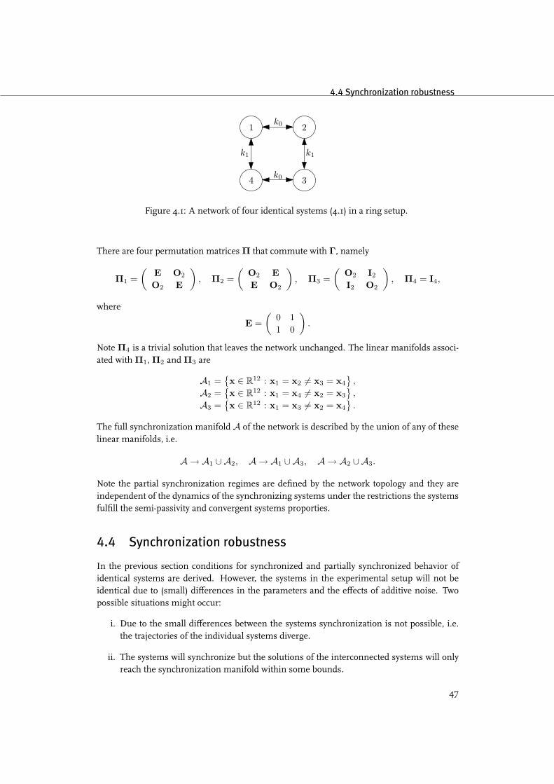
4.4 Synchronization robustness
1 2k0
4 3k0
k1k1
Figure 4.1: A network of four identical systems (4.1) in a ring setup.
There are four permutation matrices Π that commute with Γ, namely
Π1 =(
E O2
O2 E
), Π2 =
(O2 EE O2
), Π3 =
(O2 I2
I2 O2
), Π4 = I4,
where
E =(
0 11 0
).
Note Π4 is a trivial solution that leaves the network unchanged. The linear manifolds associ-ated with Π1, Π2 and Π3 are
A1 =x ∈ R12 : x1 = x2 6= x3 = x4
,
A2 =x ∈ R12 : x1 = x4 6= x2 = x3
,
A3 =x ∈ R12 : x1 = x3 6= x2 = x4
.
The full synchronization manifold A of the network is described by the union of any of theselinear manifolds, i.e.
A → A1 ∪ A2, A → A1 ∪ A3, A → A2 ∪ A3.
Note the partial synchronization regimes are defined by the network topology and they areindependent of the dynamics of the synchronizing systems under the restrictions the systemsfulfill the semi-passivity and convergent systems proporties.
4.4 Synchronization robustness
In the previous section conditions for synchronized and partially synchronized behavior ofidentical systems are derived. However, the systems in the experimental setup will not beidentical due to (small) differences in the parameters and the effects of additive noise. Twopossible situations might occur:
i. Due to the small differences between the systems synchronization is not possible, i.e.the trajectories of the individual systems diverge.
ii. The systems will synchronize but the solutions of the interconnected systems will onlyreach the synchronization manifold within some bounds.
47
4. Synchronization of Hindmarsh-Rose neurons: General theory
In this section it is shown that the synchronization error between two Hindmarsh-Rose sys-tems is bounded for t sufficiently large, i.e.
‖ x(t) ‖≤ ε,
where x = x1 − x2 and constant ε > 0. This case will be referred to as practical synchroniza-tion.
Suppose the systems (4.1) do not have the same parameter values and the states and outputsare corrupted with noise. For convenience, these systems will be written in the more generalform
xi = g(xi,θi) + Bui + ωi(t),yi = Cxi + νi(t),
(4.17)
where xi = [xi, yi, zi]T ∈ R3 are the states of the ith systems, θi ∈ R14 is the vector
containing the models parameters, ui ∈ R is the input, yi ∈ R is the models output, smoothfunctions g : R3 × R14 → R3 and matrices B and C are of appropriate dimensions. Thefunctions ωi(t) and νi(t) represent the internal noise and the output noise, respectively. Lettwo systems (4.17) be diffusively coupled with coupling strength k, then the error dynamicsare given by:
˙x = g(x1,θ1)− g(x2,θ2)− 2kB (Cx− ν(t)) + ω(t), (4.18)
where ν(t) = ν1(t)− ν2(t) and ω(t) = ω1(t)− ω2(t). Given the Hindmarsh-Rose model islinear in its parameters, (4.18) can be written with respect to the set of nominal parameters θ
as˙x = g(x,θ) +
∂g∂θ
∆θ − 2kB (Cx− ν(t)) + ω(t), (4.19)
with ∆θ is the vector containing the parameter differences with respect to the nominal pa-rameter set.
Proposition 4.4.1. Let k > kmin for kmin as defined in (4.15) then the solutions of two diffusivelycoupled non-identical Hindmarsh-Rose oscillators (4.17) satisfy the following:
limt→∞
‖ x(t) ‖≤√
gz
rs
c2
c1Ξ,
where Ξ ∈ (0, 1) and
c1 = min
(2k − b2
a− ϕ1 −
d2
8aλ1λ2
(gy −
2aλ2
d2ϕ3
)2)
,
(2aλ2
d2(β − λ1 − λ2)
),(gz
s
),
c2 = max
(‖ σx(t) + 2kνx(t) ‖∞) ,
(2aλ2
d2‖ σy(t) ‖∞
),(gz
rs‖ σz(t) ‖∞
),
with
[σx(t), σy(t), σz(t)]T =
∂g(x(t))∂θ
∆θ + ω(t).
Proof. The proof is provided in Appendix B.3.
48

4.5 Synchronization and graph topology
0 5 10 15 20 25 30 35 40 45 500
0.1
0.2
0.3
0.4
0.5
0.6
0.7
0.8
0.9
k
||x|| ∞
Figure 4.2: The maximal synchronization error ‖ x ‖∞ as function of the coupling strengthfor σx(t) = σy(t) = 1
r σz(t) = 0.05 · sin(
π10 t)and different νx(t) where the circles () denote
the case where no output noise is present νx(t) = 0, the stars (∗) indicate the synchronizationerror bound for ‖ νx(t) ‖∞≤ 0.1 and the plus signs (+) show the graph for ‖ νx(t) ‖∞≤ 0.2.
The result of Proposition 4.4.1 will give an overestimation of the error bounds obtainedthrough simulations. However it shows how the error in the synchronized states is affected bythe coupling strength and the effects of parameter mismatches and noise. It can be concludedthat:
i. the total maximal synchronization error will increase if ‖ σx(t) ‖∞, ‖ σy(t) ‖∞, ‖σz(t) ‖∞ or ‖ νx(t) ‖∞ increase,
ii. if output noise is present, νx(t) 6= 0, there exists a positive number k′ ≥ kmin such thatfor kmin ≤ k ≤ k′ the total synchronization error is decreasing while for k > k′ thetotal synchronization error is increasing,
iii. if no output noise is present, νx(t) = 0, the maximal error will decrease for kmin ≤ k ≤k′ and not increase for k > k′. Thus for a large k the disturbance rejection is maximal.
Figure 4.2 shows the error norms of the states obtained from simulations with two identicalHindmarsh-Rose oscillators with σx(t) = σy(t) = 1
r σz(t) = 0.05 · sin(
π10 t)and different
νx(t). These results support the conclusions drawn from Proposition 4.4.1.
4.5 Synchronization and graph topology
Given that two mutually coupled oscillators will synchronize there are several methods toderive conditions on the coupling strength to ensure synchronization of all oscillators in an
49
4. Synchronization of Hindmarsh-Rose neurons: General theory
arbitrary network. In this section two different methods are explained. At the end an exampleis presented that shows how both methods can be applied.
4.5.1 Wu-Chua conjecture
The Wu-Chua conjecture uses the fact that all information of the interconnections of the cou-pled oscillators is contained in the coupling matrix Γ. The conjecture states that the couplingneeded to synchronize an array of systems is inverse proportional to the smallest nonzeroeigenvalue of Γ, which implies the that the coupling required to synchronize all systems in anetwork can be derived from the coupling strength that is needed to synchronize two systems(Wu and Chua, 1996). This can be formulated as follows
µ1α1 = µ2α2,
where µi, i = 1, 2 are the smallest nonzero eigenvalues of the coupling matrix Γi and αi arethe corresponding coupling strengths. It is shown that the Wu-Chua conjecture is wrong ingeneral (Pecora, 1998) for coupled systems that show desynchronization bifurcations such asthe so-called short-wavelength bifurcations (Heagy et al., 1995). However, due to the fact thatdesynchronization bifurcations do not occur in arrays of coupled Hindmarsh-Rose neurons,see Proposition 4.2.4 for a proof, the Wu-Chua conjecture holds in this case.
4.5.2 Connection Graph Stability (CGS) method
Whereas theWu-Chua conjecture uses the smallest nonzero eigenvalue of the couplingmatrixto determine stability of the network, the Connection Graph Stability method as proposed in(Belykh et al., 2004) provides a less mathematical approach to examine stability. The CGSmethod uses the total length of shortest paths through a edge in the connection graph incombination with the number of nodes to give a bound for the minimal coupling. This isformulated in the following theorem:
Theorem 4.5.1. (Belykh et al., 2005b) The synchronization manifold of the system (4.1) is globallyasymptotically stable if
k >2k2
nbe(n, m), e = 1, . . . ,m, (4.20)
where k2 is the coupling strength sufficient for the global synchronization of two oscillators. Thequantity bε(n, m) =
∑nj>i;e∈Pij
|Pij | is the sum of the lengths of all chosen paths Pij which passthrough a given edge e that belongs to the coupling graph.
To clarify Theorem 4.5.1, an example is presented in the next subsection to show how thetheorem can be applied.
4.5.3 Example
The following example will illustrate both the Wu-Chua conjecture and the CGS method for agiven network consisting of four nodes.
50
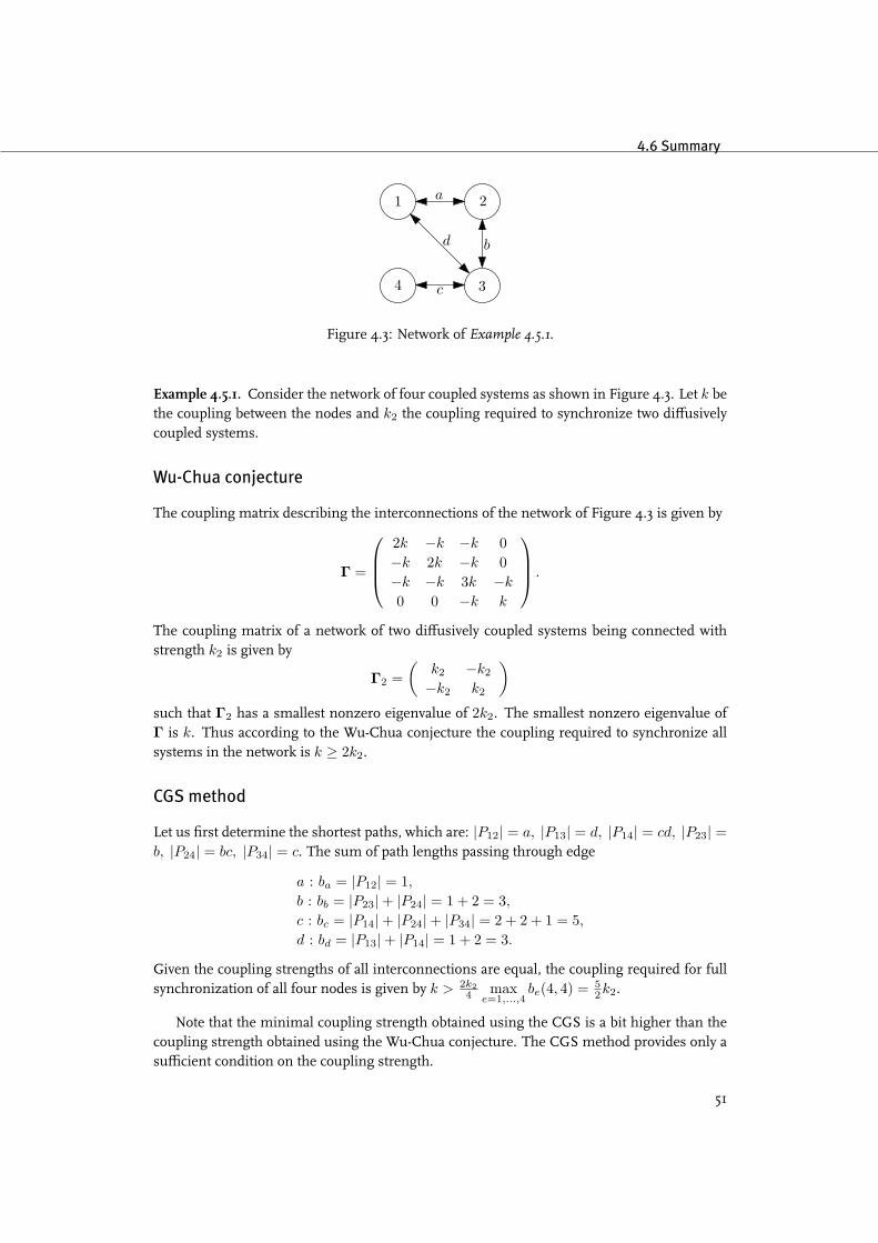
4.6 Summary
a
b
c
d
1 2
34
Figure 4.3: Network of Example 4.5.1.
Example 4.5.1. Consider the network of four coupled systems as shown in Figure 4.3. Let k bethe coupling between the nodes and k2 the coupling required to synchronize two diffusivelycoupled systems.
Wu-Chua conjecture
The coupling matrix describing the interconnections of the network of Figure 4.3 is given by
Γ =
2k −k −k 0−k 2k −k 0−k −k 3k −k
0 0 −k k
.
The coupling matrix of a network of two diffusively coupled systems being connected withstrength k2 is given by
Γ2 =(
k2 −k2
−k2 k2
)such that Γ2 has a smallest nonzero eigenvalue of 2k2. The smallest nonzero eigenvalue ofΓ is k. Thus according to the Wu-Chua conjecture the coupling required to synchronize allsystems in the network is k ≥ 2k2.
CGS method
Let us first determine the shortest paths, which are: |P12| = a, |P13| = d, |P14| = cd, |P23| =b, |P24| = bc, |P34| = c. The sum of path lengths passing through edge
a : ba = |P12| = 1,
b : bb = |P23|+ |P24| = 1 + 2 = 3,
c : bc = |P14|+ |P24|+ |P34| = 2 + 2 + 1 = 5,
d : bd = |P13|+ |P14| = 1 + 2 = 3.
Given the coupling strengths of all interconnections are equal, the coupling required for fullsynchronization of all four nodes is given by k > 2k2
4 maxe=1,...,4
be(4, 4) = 52k2.
Note that the minimal coupling strength obtained using the CGS is a bit higher than thecoupling strength obtained using the Wu-Chua conjecture. The CGS method provides only asufficient condition on the coupling strength.
51

4. Synchronization of Hindmarsh-Rose neurons: General theory
4.6 Summary
In this chapter the theory of synchronization is discussed. First the notions of semi-passivesystems and convergent systems are introduced and it is showed that the Hindmarsh-Rosemodel satisfies these conditions. Then, according to Theorems 4.2.1 and 4.3.1, mutually cou-pled Hindmarsh-Rose systems should, for sufficiently strong interconnections, show full orpartial synchronous behavior. Furthermore the influences of noise and uncertainties on thesynchronization are investigated. Finally it is showed how one can extend the synchronizationof two coupled oscillators to synchronized motion of all oscillators in networks consisting of(much) more nodes.
52
Chapter 5
Synchronization of Hindmarsh-Roseneurons: Simulations and experiments
In this chapter the theoretical results as presented in the previous chapter are validated withsimulations and experiments. In order to specify the coupling between the nodes in the exper-imental setup, a synchronization interface is developed that is build around a microcontroller.The coupling functions are defined in the microcontroller such that a wide variety of networktopologies and specific coupling functions can easily be implemented. More details of thesynchronization interface are provide in Appendix C.2.
5.1 Preliminaries
Since in the experimental setup the systems are not completely identical and the systems’outputs are possibly corrupted with noise, synchronization in the sense of Definition 4.1.1is not possible. The experimental systems are said to (partially) synchronize if the followingweakened version of Definition 4.1.1 is satisfied:
Definition 5.1.1 (Practical synchronization and practical partial synchronization with boundδ). Let xi = [xi, yi, zi]
T be the states of a system (4.1). The solutions x1(t), . . .xk(t) of thek coupled systems (4.1) with initial conditions x1(0), . . .xk(0) ∈ R3k are called practically(partially) synchronized with bound δ if
limt→∞
‖ xi(t)− xj(t) ‖≤ δ
for all t ∈ R+, δ > 0 and all (some) i, j = 1, . . . , k.
During the experiments maximal four channels are available for the recording of data.Therefore it is chosen to record solely the x-sates of the systems since these states can beregarded as the natural outputs of the Hindmarsh-Rosemodel. Definition 5.1.1 now, obviously,only applies to errors between the x-states. In this case the experimental systems are calledsynchronized when δ ≤ 0.5. Although this value for δ seems to be rather high, one has tonotice that, due to particular shape of the spikes, a small mismatch between the spikes willresult in a large error.
53
5. Synchronization of Hindmarsh-Rose neurons: Simulations and experiments
0 0.5 1 1.5 2
−2
0
2
time [s]
x1−
x2
[V]
0 0.5 1 1.5 2
−2
0
2
time [s]
x1−
x2
[V]
0 0.5 1 1.5 2
−2
0
2
time [s]
x1−
x2
[V]
Figure 5.1: Error between the two practically synchronized Hindmarsh-Rose circuits. Toppanel – Simulation k = 0.5, middle panel – Experiment k = 0.6, bottom panel – Experimentk = 1.2
5.2 Two systems
First the most obvious case is investigated, i.e. the synchronization of two coupled systems.The two systems are mutually coupled with coupling strength k.
Simulations are performed in order to obtain the minimal coupling kmin that is requiredto synchronize the systems. It turned out that for kmin = 0.5 both systems’ outputs aresynchronized. This value is less than the analytical minimal coupling strength that is derivedin Proposition 4.2.4. This difference can be explained since the result of Proposition 4.2.4 isobtained using a conservative Lyapunov function argument, i.e. only a sufficient condition forthe existence of the synchronized state is provided.
The systems in the experimental setup are found to practically synchronize for a couplingk > kmin = 0.6. The error between the first states of the circuits for both the simulation asthe experiment are shown in Figure 5.1. Here the vertical line indicates the moment that thesynchronization is turned on.
From this figure one can see that in the experimental setup some small error will remain.Comparing the figure in the middle panel with the figure in the bottom panel it is clear thatthis error decreases when k is increased, which is confirming the result of Proposition 4.4.1.
54
5.4 Four systems
1
32 k3
k2k1
(a)
1 2
34
k1
k2
k3
k4
k5 k6
(b)
Figure 5.2: Three (5.2(a)) and four (5.2(b)) interconnected Hindmarsh-Rose systems
5.3 Three systems
The next experiment is to synchronize three Hindmarsh-Rose neurons. The schematic setupof this experiment is shown in Figure 5.2(a).
The three systems can be coupled in a line, e.g. k1, k2 6= 0, k3 = 0, or a fully connectedgraph can be considered where k1, k2, k3 6= 0. In both cases the nonzero couplings betweenthe nodes is chosen with equal strength, i.e. every active coupling is of strength k.
Given that the minimal coupling that synchronizes two systems, denoted by k2, is known,the required coupling strength for both configuration with three systems can be computedusing the Wu-Chua conjecture or the CGS method (see Section 4.5).
The three systems that are coupled in a line will synchronize for k ≥ 2k2 according to boththe Wu-Chua conjecture and the CGS method. Indeed, simulations show that the systemssynchronize for k ≥ 1. In the experimental setup a coupling k > 1.2 is required to achievesynchronization.
When a connection is added to the previous configuration, i.e. the graph of the three sys-tems is fully connected, the systems should synchronize with a less strong coupling. Applyingboth the Wu-Chua conjecture and the CGS, the minimal required coupling k ≥ 2
3k2 is found.Both the simulations (k ≥ 1
3 ) and the experiments (k ≥ 0.4) support this finding.The results with the different configurations show how adding (or losing) a connection
drastically changes the amount of coupling that is necessary. Plots of the synchronization ofthe three systems in the two configurations are provided in Appendix E.2.
5.4 Four systems
Consider four systems that are connected as depicted in Figure 5.2(b). The four systems canbe coupled in various configurations:
i. Ring (k1, k2, k3, k4 6= 0, k5, k6 = 0),
ii. Ring with diagonal (k1, k2, k3, k4, k5 6= 0, k6 = 0),
iii. Fully connected graph (k1, k2, k3, k4, k5, k6 6= 0),
55
5. Synchronization of Hindmarsh-Rose neurons: Simulations and experiments
iv. Network of Example 4.5.1 (k1, k2, k3, k5 6= 0, k4, k6 = 0),
v. Line (k1, k2, k3 6= 0, k4, k5, k6 = 0).
Next (partial) synchronization for these different configurations will be discussed. Forgraphical representations of the synchronous state, e.g. plots of the error signals, the readeris referred to Appendix E.2.
5.4.1 Full synchronization
At first it is investigated what coupling is needed such that all systems in the network dosynchronize for the various configurations. For all configurations the strength of the activeinterconnections, i.e. ki 6= 0, i = 1, . . . 6, are chosen identical.
Ring
The coupling matrix corresponding to the four systems that are coupled in a ring is given by
Γ =
2k −k 0 −k
−k 2k −k 00 −k 2k −k
−k 0 −k 2k
,
such that the smallest nonzero eigenvalue of Γ is given by 2k. Following the Wu-CHua con-jecture, the coupling required to synchronize the four systems is k ≥ k2. However, applyingthe CGS method, one finds that k ≥ 3
2k2. Simulations show that the synchronous state isreached for k ≥ 0.5 which means that the Wu-Chua conjecture in this case provides the exactamount of coupling that is required and the CGS method gives an overestimation. In theexperimental setup k ≥ 0.6 is found. Figure 5.3 shows the errors between the first states ofthe systems for this setup.
Ring with diagonal
In order to improve synchronization, i.e. there is a less strong coupling strength necessaryto synchronize the systems, one can think of adding an extra connection. Nevertheless, us-ing the CGS method it can easily be showed that adding solely this extra connection has nouse. Denoting the edge between the systems 1 and 2 with a, the sum of the shortest pathsthrough this edge is given by ba = 3. This is equal to the sum of shortest paths that arepassing through this same edge in the ring configuration. Therefore, the minimal couplingrequired for synchronization in this particular configuration is identical to the one in the ringconfiguration, i.e. k ≥ 3
2k2. The Wu-Chua conjecture gives the same result as is found in thering setup as well. Even the required coupling strength that are found in the simulations andexperiments are identical for both configurations. Adding such an extra connection is thususeless when one wants to achieve full synchronization.
56

5.4 Four systems
0 1 2
−2
0
2
time [s]
x1−
x2
[V]
0 1 2
−2
0
2
time [s]
x1−
x3
[V]
0 1 2
−2
0
2
time [s]
x1−
x4
[V]
0 1 2
−2
0
2
time [s]
x2−
x3
[V]
0 1 2
−2
0
2
time [s]
x2−
x4
[V]
0 1 2
−2
0
2
time [s]
x3−
x4
[V]
Figure 5.3: Error between the states of four practically synchronized Hindmarsh-Rose circuitsin the ring setup for k = 0.6. The vertical line indicates to instance of time that the synchro-nization is turned on.
Fully connected
In the case that the ring with diagonal configuration is augmented with the other extra con-nection, the graphs becomes fully connected. Therefore the systems will all synchronize withminimal effort. Both the Wu-Chua conjecture and the CGS method give k ≥ 1
2k2. Thesimulation with this configuration follows these results, i.e. k ≥ 0.25. However, in the ex-perimental setup some extra coupling is required, k ≥ 0.33. Probably the influence of thesmall differences between the circuits is somewhat larger than it is in the other configura-tions. Note that both the Wu-Chua conjecture and the GCS method assume that the systemsunder consideration are identical.
Network of Example 4.5.1
As shown in Example 4.5.1, the minimal coupling according to the Wu-Chua conjecture isk ≥ 2k2 and the GCS method shows k ≥ 5
2k2. According to the simulation the Wu-Chuaconjecture is also in this case the one to use, i.e. k ≥ 1. In the experiments k ≥ 1.1 is found.
Notice the large difference in terms of coupling strength between this network and thethree fully connected systems or the four systems connected in a ring with diagonal. Theconnection between the nodes 3 and 4 is definitely the weakest link such that removing thisconnection or adding a connection between the systems 1 and 4 will improve the synchroniza-tion a lot.
57

5. Synchronization of Hindmarsh-Rose neurons: Simulations and experiments
Line
In the situation where the four systems are coupled in a line is the worst configuration interms of synchronization since the distance between nodes 1 and 4 is maximal. This meansthat first the systems 1 and 2 have to synchronize, next the systems 2 and 3, and finally thesystems 3 and 4. Therefore a strong coupling between the nodes is necessary.
Applying the Wu-Chua conjecture one finds that k ≥ (2 +√
2)k2. The CGS methodimplies that even a larger coupling is required to have full synchronization. The sum of allshortest path lengths through the edge between the nodes 2 and 3 is b1−2 = 8, and thereforek ≥ 4k2. According to the outcome of the simulations the coupling to fully synchronize thefour systems in the line configuration should be k ≥ 1 + 1
2
√2, which confirms the result of
the Wu-Chua conjecture. In the experimental setup synchronization is found for k ≥ 2.2.
5.4.2 Partial synchronization
In the networks of the configurations i-iii are, depending on the coupling, some symmetriespresent. Therefore partial synchronization regimes can exist.
Ring
There are symmetries present in the ring configuration in the case that the couplings arechosen as
k1 = k3 = k′, k2 = k4 = k?.
This case is identical to Example 4.3.1 such that the the manifolds that describe the partialsynchronization regimes are given by
A1 =x ∈ R12 : x1 = x2 6= x3 = x4
,
A2 =x ∈ R12 : x1 = x4 6= x2 = x3
,
A3 =x ∈ R12 : x1 = x3 6= x2 = x4
.
The eigenvalues of the coupling matrix are γ1 = 0, γ2 = min 2k′, 2k?, γ3 = max 2k′, 2k?and γ4 = 2 (k′ + k?). Hence, using Theorem 4.3.1, for 2k′ ≥ γ > 2k? a subset of the setA1 is asymptotically stable and for 2k? ≥ γ > 2k′ a subset of the set A2 is asymptoticallystable. The subset of the set A3 can only be stable as the intersection of A1 and A2. However,this intersection described full synchronization of the network and therefore the set A3 willnot define a regime of partial synchronization. The stability diagram of the four systems isshowed in Figure 5.4.
In the simulations the value γ = 1 is found where in the experimental setup γ = 1.2.Figure 5.5 shows the experimental result for partial synchronization with respect to the setA2
for k′ = 0.3 and k? = 0.6.
Ring with diagonal
This network has a symmetry when the following coupling between the nodes is used
k1 = k2 = k′, k2 = k4 = k?, k5 = k].
58
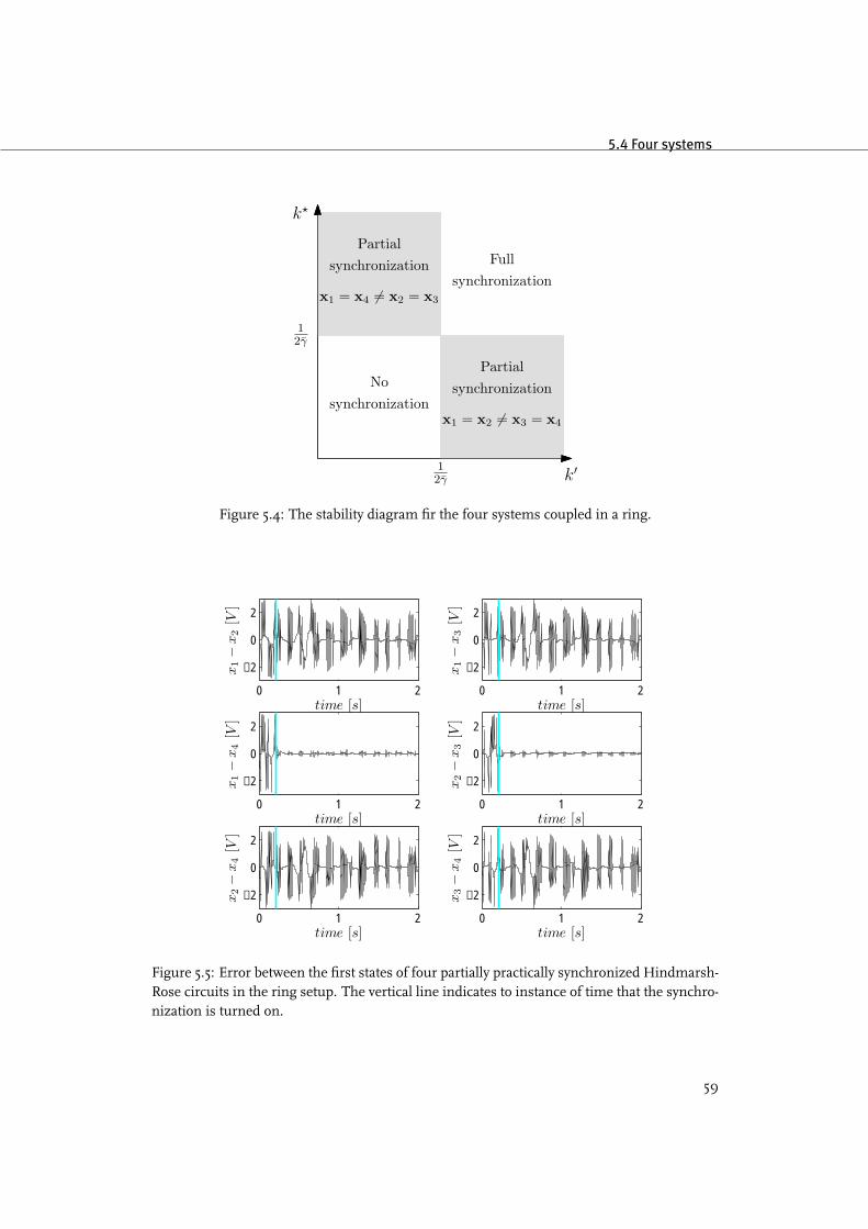
5.4 Four systems
x1 = x4 6= x2 = x3
x1 = x2 6= x3 = x4
Partialsynchronization
Partialsynchronization
x1 = x4 6= x2 = x3
x1 = x2 6= x3 = x4
Partialsynchronization
Partialsynchronization
Fullsynchronization
Nosynchronization
12γ
12γ
k′
k?
Figure 5.4: The stability diagram fir the four systems coupled in a ring.
0 1 2
−2
0
2
time [s]
x1−
x2
[V]
0 1 2
−2
0
2
time [s]
x1−
x3
[V]
0 1 2
−2
0
2
time [s]
x1−
x4
[V]
0 1 2
−2
0
2
time [s]
x2−
x3
[V]
0 1 2
−2
0
2
time [s]
x2−
x4
[V]
0 1 2
−2
0
2
time [s]
x3−
x4
[V]
Figure 5.5: Error between the first states of four partially practically synchronized Hindmarsh-Rose circuits in the ring setup. The vertical line indicates to instance of time that the synchro-nization is turned on.
59

5. Synchronization of Hindmarsh-Rose neurons: Simulations and experiments
The coupling matrix is given by
Γ =
k′ + k? −k′ 0 −k?
−k′ k′ + k? + k] −k] −k?
0 −k? k′ + k? −k′
−k? −k] −k′ k′ + k? + k]
,
and the eigenvalues of Γ are γ1 = 0, γ2 = 2 (k′ + k?) , γ3 = k′+k?+k]−√
(k? − k′)2 + k] 2
and γ4 = k′ + k? + k] +√
(k? − k′)2 + k] 2. Note that since γ4 > γ3 and following Theorem4.2.1 all systems will synchronize if γ2 ≥ γ and γ3 ≥ γ.
One matrix can be found that commutes with Γ, namely
Π1 =(
O2 I2
I2 O2
).
Applying Theorem 4.3.1, there exists a subset of the set
A1 =x ∈ R12 : x1 = x3 6= x2 = x4
that is asymptotically stable if the following condition is satisfied:
2 (k′ + k?) < γ ≤ k′ + k? + k] −√
(k? − k′)2 + k] 2. (5.1)
However, inequality (5.1) implies
k] − k′ − k? −√
(k? − k′)2 + k] 2> 0,
which is a contradiction since k′, k?, k] > 0. Therefore no values to the couplings can beassigned that ensure stability of this partial synchronization regime, i.e. this particular partialsynchronization regime does not exist.
When k′ = k?, some additional symmetries appear in the network. The followingmatricescommute with the corresponding coupling matrix
Π2 =
0 0 1 00 1 0 01 0 0 00 0 0 1
, Π3 =
1 0 0 00 0 0 10 0 1 00 1 0 0
,
such that the following sets might have a asymptotically stable subset
A2 =x ∈ R12 : x1 = x3 6= x2 6= x4
,
A3 =x ∈ R12 : x2 = x4 6= x1 6= x3
.
The smallest nonzero eigenvalues of Γ for permutation Π2 is γ2 = 2k′ and for permutationΠ3 one finds γ2 = 2
(k′ + k]
). Note that the eigenvalue γ2 = 2k′ corresponding to Π2
provides the same condition on the coupling strength as is found for full synchronization.This implies that the partial synchronization regime that is given by Π2 intersects with thefully synchronized state such that this partial synchronization regime actually can not exist.The setA3 however contains a asymptotical stable subset for γ2 = 2
(k′ + k]
)≥ γ > 4k′ with
in the simulations γ = 1 and in the experimental setup γ = 1.2.
60

5.5 Summary
Fully connected
For the fully connected graph the following coupling between the nodes is chosen as
k1 = k2 = k′, k2 = k4 = k?, k5 = k6 = k].
The coupling matrix for this configuration commutes with the same permutation matricesthat are found in the ring setup. Therefore the same possibly asymptotically stable sets areobtained:
A1 =x ∈ R12 : x1 = x2 6= x3 = x4
,
A2 =x ∈ R12 : x1 = x4 6= x2 = x3
,
A3 =x ∈ R12 : x1 = x3 6= x2 = x4
.
It follows immediately that for k] small, the situation is identical to the ring setup. However,for this configuration there exists a asymptotically stable subset of the setA3 when 2k] ≥ γ >
2 (k′ + k?). In the simulations γ = 1 is found whereas for the experiments γ = 1.2.
5.5 Summary
In this chapter the theoretical results of Chapter 4 are validated with both simulations andexperiment for various networks consisting of up to four systems. The coupling that is re-quired for the synchronization of two system is found to be k2 = 0.5 for the simulations andk2 = 0.6 in the experimental setup. This difference is due to the fact that the systems are notcompletely identical.
Using these results an extension is made for networks consisting of more systems withthe methods as described in Section 4.5. The Wu-Chua conjecture provides in all cases theright amount of coupling that is necessary for synchronization whereas the CGS methodsometimes gives an overestimation. Table 5.1 gives an overview of the minimal couplingstrength for both the simulations and the experiments for the various configurations.
For the four coupled systems partial synchronization is noticed. The regimes that arefound analytically and in the simulations do also appear in the experiments.
61
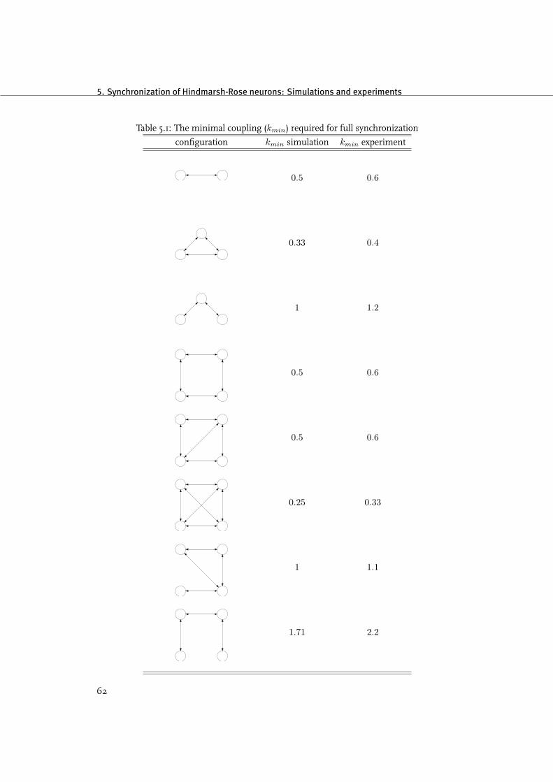
5. Synchronization of Hindmarsh-Rose neurons: Simulations and experiments
Table 5.1: The minimal coupling (kmin) required for full synchronization
configuration kmin simulation kmin experiment
0.5 0.6
0.33 0.4
1 1.2
0.5 0.6
0.5 0.6
0.25 0.33
1 1.1
1.71 2.2
62
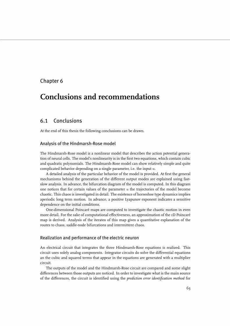
Chapter 6
Conclusions and recommendations
6.1 Conclusions
At the end of this thesis the following conclusions can be drawn.
Analysis of the Hindmarsh-Rose model
The Hindmarsh-Rose model is a nonlinear model that describes the action potential genera-tion of neural cells. The model’s nonlinearity is in the first two equations, which contain cubicand quadratic polynomials. The Hindmarsh-Rose model can show relatively simple and quitecomplicated behavior depending on a single parameter, i.e. the input u.
A detailed analysis of the particular behavior of the model is provided. At first the generalmechanisms behind the generation of the different output modes are explained using fast-slow analysis. In advance, the bifurcation diagram of the model is computed. In this diagramone notices that for certain values of the parameter u the trajectories of the model becomechaotic. This chaos is investigated in detail. The existence of horseshoe type dynamics impliesaperiodic long term motion. In advance, a positive Lyapunov exponent indicates a sensitivedependence on the initial conditions.
One-dimensional Poincaré maps are computed to investigate the chaotic motion in evenmore detail. For the sake of computational effectiveness, an approximation of the 1D Poincarémap is derived. Analysis of the iterates of this map gives a quantitative explanation of theroutes to chaos, saddle-node bifurcations and intermittent chaos.
Realization and performance of the electric neuron
An electrical circuit that integrates the three Hindmarsh-Rose equations is realized. Thiscircuit uses solely analog components. Integrator circuits do solve the differential equationsan the cubic and squared terms that appear in the equations are generated with a multipliercircuit.
The outputs of the model and the Hindmarsh-Rose circuit are compared and some slightdifferences between those outputs are noticed. In order to investigate what is the main sourceof the differences, the circuit is identified using the prediction error identification method for
63

6. Conclusions and recommendations
the slow subsystem and extended Kalman filtering for the fast subsystem. Simulating withthe identified model show that the differences in the output of the original Hindmarsh-Rosemodel and the circuit are due to small deviations in the parameter values.
In total four electromechanical Hindmarsh-Rose neurons are realized.
Synchronization of Hindmarsh-Rose neurons
The synchronous behavior of the Hindmarsh-Rose neurons is investigated. Each systems iscoupled to other systems using a mutual, or bidirectional, coupling via the first state.
A theoretical framework that guarantees the existence of (partial) synchronization regimesin diffusively coupled networks is discussed. Using a semi-passivity condition, this frameworkprovides sufficient conditions for the existence of full and partial synchronization of mutuallydiffusively coupled systems. It is proved that the Hindmarsh-Rose system satisfies the semi-passivity condition and therefore the coupled systems should synchronize under the conditionthat the strength of the coupling is large enough.
The effects of parameter mismatches between the individual systems and other sourcesof noise on the synchronization are investigated. It is shown that increasing the couplingstrength will first reduce the amount of error between the systems. However, if output noiseis present, the error will finally increase for increasing coupling strength.
An analytical expression for the minimal coupling that guarantees synchronization of twosystems is presented. In addition, two different methods are coined, i.e. the Wu-Chua conjec-ture and the CGS method, that can be used to extend the result of the two coupled system tonetworks that contain a larger number of systems and have different topologies.
Finally, simulations and experiments are performed that satisfy the theoretical results andshow the existence of (partial) synchronization for up to four systems in different configu-rations. In the experimental setup a microcontroller based interface is used to define thecoupling functions.
6.2 Recommendations
A number of recommendation can be made for further research.
Recommendations regarding the experimental setup
At first the experimental setup can be somewhat improved. The current setup does rely very onthe power source since the constant parameters in the circuits are directly related to the voltagethat is supplied by the power unit. To overcome this problem voltage stabilizing circuits canbe implemented on each individual circuit.
Since a microcontroller synchronization interface is used, a conversion from analog sig-nals to digital signals and visa versa has to be made. The problem with this experimental setupis that the voltage range of the analog-digital converters does not match with the range of theoutput of a circuit. Therefore additional signal reshaping is necessary. It is, however, possibleto choose the parameters of the model in such a way that the output is within the range ofthe analog-digital converter while the particular dynamical behavior is not changed. Anotherpossibility is to use a different type of analog-digital converter which has a wider input range.
64
6.2 Recommendations
Possible future research
In this thesis only diffusively coupled network of a limited number of systems is investigated.A first logical step for further research is to extend the number of systems. With a largernumber of systems many more topologies can be examined.
One can also think of adding time delays in the transmitted signals, see for instance (Hui-jberts et al., 2007). Because a microcontroller is used to define the coupling functions, a delaycan easily be established by buffering signals.
Furthermore, the effect of different types of couplings can be investigated. A first candi-date would be the Fast Threshold Modulation (FTM) coupling as described in (Somers andKopell, 1993). This type of coupling represents a more realistic signal transmission betweenindividual neurons, i.e. chemical synapses, see (Koch, 1999) for instance. This type of cou-pling is however not continuous, and therefore mathematical analysis of networks with theFTM coupling can be a real challenge.
Finally, one can think of performing more complex experiments with the electromechan-ical neurons. As shown by (Szücs et al., 2000) it is possible to let electronic neurons interactwith "real" biological neurons. This in combination with the ability to identify neural dynam-ics from measurements (Steur et al., 2007) might offer, for instance, the possibility supplysubstitutes for failing neurons.
65

6. Conclusions and recommendations
66

Bibliography
Belykh, Igor, Enno de Lange andMartinHasler (2005a). Synchronization of bursting neurons:What matters in the network topology. Physical Review Letters 94, 188101–1 – 188101–4.
Belykh, Igor, Martin Hasler, Menno Lauret and Henk Nijmeijer (2005b). Synchronization andgraph topology. Int. J. Bif. and chaos 15, 3423–3433.
Belykh, Vladimir, Igor Belykh and Erik Moskilde (2005c). The hyperbolic Plykin attractor canexist in neuron models. Int. J. Bif. and chaos 15, 3567–3578.
Belykh, Vladimir N., Igor V. Belykh and Martin Hasler (2004). Connection graph stabilitymethod for synchronized coupled chaotic systems. Physica D 195, 159–187.
Belykh, V.N., I.V. Belykh, M. Colding-Jørgensen and E. Mosekilde (2000). Homoclinic bifur-cations leading to the emergence of bursting oscillations in cell models. Euro. Phys. J. E3, 205–219.
Bertsekas, Dimitri P. (1996). Incremental least squares mothods and the extended Kalmanfilter. Siam J. Optimization 6, 807–822.
Bullock, Thomas H., Michela V. Bennet, Daniel Johnston, Robert Josephson, Eve Marder andR. Douglas Fields (2005). The Neuron Doctorine, Redux. Science 310, 791–793.
Cymbalyuk, Gennady S., Ronald L. Calabrese and Andrey L. Shilnikov (2005). How a neu-ron model can demonstrate co-existence of tonic spiking and bursting. Neurocomputing 65-66, 869–875.
Devany, Robbert L. (1986). An introduction to chaotic dynamical systems. The Ben-jamin/Cummings Publishing co., inc.
Dyson, Freeman J. (1996). Book review: Nature’s numbers by ian stewart. The AmericanMath-ematical Monthly 7, 610–612.
FitzHugh, R. (1961). Impulses and physiological states in theoretic models of nerve mem-brane.. Biophys. J. 1, 445–466.
Gelb, Arthur, Ed. (1996). applied optimal estimation. 14 ed.. The M.I.T press.
Gong, Pulin and Cees van Leeuwen (2007). Dynamically Maintained Spike Timing Sequencesin Networks of Pulse-Coupled Oscillators with Delays. Physical Review Letters.
67

Bibliography
Gray, Charles M. (1994). Synchronous Oscillations in Neuronal Systems: Mechanisms andFunctions. Journ. Comp. Neuroscience 1, 11–38.
Guckenheimer, John and Philip Holmes (1983). Nonlinea Oscillations, Dynamical Systems, andBifurcations of Vector Fields. Springer-Verlag.
Heagy, James F., LouisM. Pecora and Thomas L. Carroll (1995). Short wavelength bifurcationsand size instabilities in coupled oscillator systems. Physical Review Letters 74, 4185–4188.
Hindmarsh, J. L. and R. M. Rose (1982). A model of the nerve impulse using two first-orderdifferential equations. Nature 296, 162–164.
Hindmarsh, Jim and Philip Cornelius (2005). BURSTING. Chap. 1. World Scientific.
Hindmarsh, J.L. and R.M. Rose (1984). A model for neuronal bursting using three coupleddifferential equations. Proc. R. Soc. Lond. B 221, 87–102.
Hodgkin, A.L. and A.F. Huxley (1952). A quantitave description of membrane current and itsapplication to conductance and excitation in nerve.. J. Physiol. Lond 117, 500–544.
Holden, Arun V. and Yin-Shui Fan (1992a). Crisis-induced Chaos in the Hindmarsh-RoseModel for Neuronal Activity. Chaos, Solitons and Fractals 2, 583–595.
Holden, Arun V. and Yin-Shui Fan (1992b). From Simple to Complex Bursting Oscillatory Be-haviour via Intermittent Chaos in the Hindmarsh-Rose Model for Neuronal Activity. Chaos,Solitons and Fractals 2, 349–369.
Holden, Arun V. and Yin-Shui Fan (1992c). From Simple to Simple Bursting Oscillatory Be-haviour via Chaos in the Hindmarsh-Rose Model for Neuronal Activity. Chaos, Solitons andFractals 2, 221–236.
Huijberts, Henri, Henk Nijmeijer and Toshiki Oguchi (2007). Anticipating synchronizationof chaotic Lur’e systems. Chaos 17, 013117–1 – 013117–13.
Huijberts, H.J.C., H. Nijmeijer and R.M.A. Willems (1998). A control perspective on com-munication using chaotic systems. Decision and Control, 1998. Proceedings of the 37th IEEEConference on 2, 1957–1962.
Huygens, C. (1932). Oeuvres complétes de christiaan huygens.Martinus Nijhoff. Includes worksfrom 1651-1666.
Huygens, C. (1986). Christiaan Huygens′ the pendulum or geometrical demonstrations concerningthe motion of pendula as applied to clocks (translated by R. Blackwell). Iowa State UniversityPress.
Izhikevich, E.M. (2000). Neural excitability, Spiking and Bursting. Int. J. Bifurcation and Chaos10, 1171–1266.
Izhikevich, E.M. (2004). Which Model to Use for Cortical Spiking Neurons?. IEEE Trans.Neural Networks 15, 1063–1070.
Khalil, H.K. (2002). Nonlinear Systems. 3 ed.. Prentice Hall.
68
Koch, C. (1999). Biophysics of computation. 1 ed.. Oxford University Press.
Lee, Young Jun, Jihyun Lee, Y. B. Kim, J. Ayers, A. Volkovskii, A. Selverston, H. Abarbaneland M. Rabinovich (2004). Low power real time electronic neuron VLSI design usingsubthreshold technique. Proc. of the 2004 International Symposium on Circuits and Systems4, 744–747.
Lewis, E. R. (1968). Using electronic circuits to model simple neuroelectric interactions. Pro-ceedings of the IEEE 56, 931– 949.
Li, T.Y. and J.A. Yorke (1975). Period three implies chaos. Amer. Math. Monthly 82, 985–992.
Linares-Barranco, B., E. Sanchez-Sinencio, A. Rodriguez-Vazquez and J. L. Huertas (1991). ACMOS implementation of FitzHugh-Nagumo neuron model. IEEE jour. Solid State Circuits26, 956–965.
Ljung, L. (1999). System Identification: Theory for the User. Prentice-Hall.
Lorenz, Edward N. (1963). Deterministic non-periodic flow. J. Athmos. Sci. 20, 130–141.
Merlat, L., N. Silvestre and J. Merckle (1996). AHindmarsh and Rose-based electronic burster.IEEE Proceedings of MicroNeuro ’96 pp. 39–44.
Milne, Alice E. and Zaid S. Chalabi (2001). Control analysis of the Rose-Hindmarsh modelfor neural activity. IMA Journal of Mathematics Applied in Medicine and Biology 18, 53–75.
Morris, C. and H. Lecar (1981). Voltage oscillations in the barnacle giant muscle fiber. BiophysJ. 193, 193–213.
Nagumo, J.S., S. Arimoto and S. Yoshizawa (1962). An active pulse transmission line simu-lating nerve axon.. Proc. IRE 50, 2061–2070.
Nijmeijer, H. and I. Mareels (1996). An observer looks at synchronization. IEEE Trans. CircuitsSyst. I 44, 882–890.
Ott, Edward (2002). Chaos in Dynamical Systems. 2 ed.. Cambridge University Press.
Ott, Edward, Celso Grebogi and James A. Yorke (1990). Controlling Chaos. Physical ReviewLetters 64, 1196–1199.
Oud, W. T., I. Yu. Tyukin and H. Nijmeijer (2004). Sufficient conditions for synchroniza-tion in an ensemble of hindmarsh and rose neurons: passivity-based apporach. 6th IFAC-Symposium on Nonlinear Control Systems, Stuttgart.
Pavlov, A., A. Pogromsky, N. van de Wouw and H. Nijmeijer (2004). Convergent dynamics, atribute to Boris Pavlovich Demidovich. Systems and Control Letters 52, 257–261.
Pecora, Louis M. (1998). Synchronization conditions and desymchronization patterns in cou-pled limit-cycle and chaotic systems. Physical Review E 58, 347–360.
Pecora, Louis M. and Thomas L. Carroll (1990). Synchronizatin in Chaotic Systems. PhysicalReview Letters 64, 821–825.
69

Bibliography
Pikovsky, Arkady, Michael Rosenblum and Jürgen Kurths (2003). Synchronization. 2 ed.. Cam-bridge University Press.
Pogromsky, A. Yu. (1998). Passivity based design of synchronizing systems. Int. J. Bifurcationand Chaos 8, 295–319.
Pogromsky, A. Yu. and H. Nijmeijer (2001). Cooperative Oscillatory Behavior of MutuallyCoupled Dynamical Systems. IEEE Trans. Circuits Syst. I 48, 152–162.
Pogromsky, A. Yu., G. Santoboni and H. Nijmeijer (2002). Partial synchronization: fromsymmetry towards stability. Physica D 172, 65–87.
Raffone, A. and C. van Leeuwen (2003). Dynamic synchronization and chaos in an associativeneural network with multiple active memories. Chaos 13, 1090–1104.
Raol, J.R., G. Girija and J. Singh (2004). Modelling and Parameter Estimation of DynamicalSystems. The Institution of Electrical Engineers, London.
Roy, Guy (1972). A Simple Electronic Analog of the Squid Axon Membrane: The NEUROFET.IEEE trans. on Biomedical Engineering 19, 60–63.
Ruelle, D. (1991). Chance and Chaos. Princeton University Press.
Ruelle, D. and F. Takens (1971). On the Nature of Turbulence. Commun. Math. Phys. 20, 167–192.
Schoppa, Nathan E. and Gary L. Westbrook (2001). Glomerulus-Specific Synchronization ofMitral Cells in the Olfactory Bulb. Neuron 21, 639–651.
Singer, Wolf (1999). Neuronal Synchrony: A Versitile Code for the Definition of Relations.Neuron 24, 49–65.
Smale, S. (1967). Differentiable dynamical systems. Bull. Am. Math. Soc. 73, 747–817.
Somers, David and Nancy Kopell (1993). Rapid synchronization through fast threshold mod-ulation. Biol. Cybern. 68, 393–407.
Steur, Erik, Ivan Tyukin, Cees van Leeuwen and Henk Nijmeijer (2007). Reconstructing Dy-namics of Spiking Neurons from Input-Output Measurements in Vitro. Submitted to thePhysCon 2007 conference, preprint available in Appendix F.
Strogatz, Steven H. (1994). Nonlinear Dynamics and Chaos. Addison-Wesley Publishing Com-pany.
Strogatz, Steven H. and Ian Stewart (1993). Coupled Oscillators and Biological Synchroniza-tion. Sci. Am. 269, 68–74.
Szücs, Attila, Pablo Varona, Alexander R. Volkovskii, Henry D.I. Arbabanel, Mikhail I. Rabi-novich and Allen I. Selverston (2000). Interacting biological and electronic neurons gener-ate realistic oscillatory rhythms. Neuroreport 11, 563–569.
Terman, David (1991). Chaotic Spikes Arising from a Model of Bursting in Excitable Mem-branes. SIAM J. Appl. Math. 51, 1418–1450.
70

Terman, David (1992). The Transition from Bursting to Continuous Spiking in ExcitableMembrane Models. J. Nonlinear Sci. 2, 135–182.
Tyukin, Ivan, Erik Steur, Cees van Leeuwen and Henk Nijmeijer (2006). Non-uniform small-gain theorems for systems with unstable invariant sets. Siam Journ. Control and Optimiza-tion (accepted, preprint available in Appendix F).
van der Pol, B. (1927). Forced oscillations in a circuit with nonlinear resistance. PhilosophicalMagazine 3, 65–80.
van der Steen, R. (2006). Numerical and experimental analysis of multiple Chua circuits.Technical Report DCT. 2006.015. Eindhoven University of Technology, Department of Me-chanical Engineering.
Wang, X. J. (1993). Genesis of bursting oscillations in the Hindmarsh-Rose model and homo-clinicity ot a chaotic saddle. Physica D 62, 263–274.
Willems, Jan C. (1972). Dissipative Dynamical Systems part I: General Theory. Arch. RationalMech. Anal. 45, 321–351.
Wolf, Alan, Jack B. Swift, Harry L. Swinney and John A. Vastano (1985). DeterminingLyaponuv exponents from a time series. Physica D 16, 285–317.
Wu, Chai Wah and Leon O. Chua (1996). On a conjecture regarding the synchronization inan array of linearly coupled dynamical systems. IEEE Trans. Circuits Syst. I 43, 161–165.
Xie, Yong, Jian-Xue Xu, San-Jue Hu, Yan-Mei Kang, Hong-Jun Yang and Yu-Bin Duan (2004).Dynamical mechanism for sensitive response of aperiodic firing cells to external stimula-tion. Chaos, Solitons and Fractals 22, 151–160.
71

72
Appendix A
The Approximated 1D Poincaré Map
The 1D Poincaré map as depicted in Figure 2.10 is approximated by a map as a hyperbola withtwo asymptotes L1 and L2:
L1(zn) = 0.94zn + 0.30,
L2(zn, u) = −0.35 arctan (80(zn + 1.21u− 0.68))− 1.25 + 0.8u.
The approximated model map is given by the function
(zn+1 − L1(zn)) (zn+1 − L2(zn, u)) = C,
or explicitly,
zk+1 = G(zn) =L1(zn) + L2(zn, u)
2− 1
2
√− (L1(zn)− L2(zn, u))2 − 4C, (A.1)
whereC = 0.029.
As showed in Figure A.1 the asymptotes are chosen such that the approximated map G(z)follows closely the computed Poincaré map of the Hindmarsh-Rose model on the Poincarésection Σ. When the input u is increased asymptote L2 should shift upwards and to the right.For decreasing u this asymptote moves downward and to the left. Therefore, the asymptoteL2 is a function of the bifurcation parameter u.
73
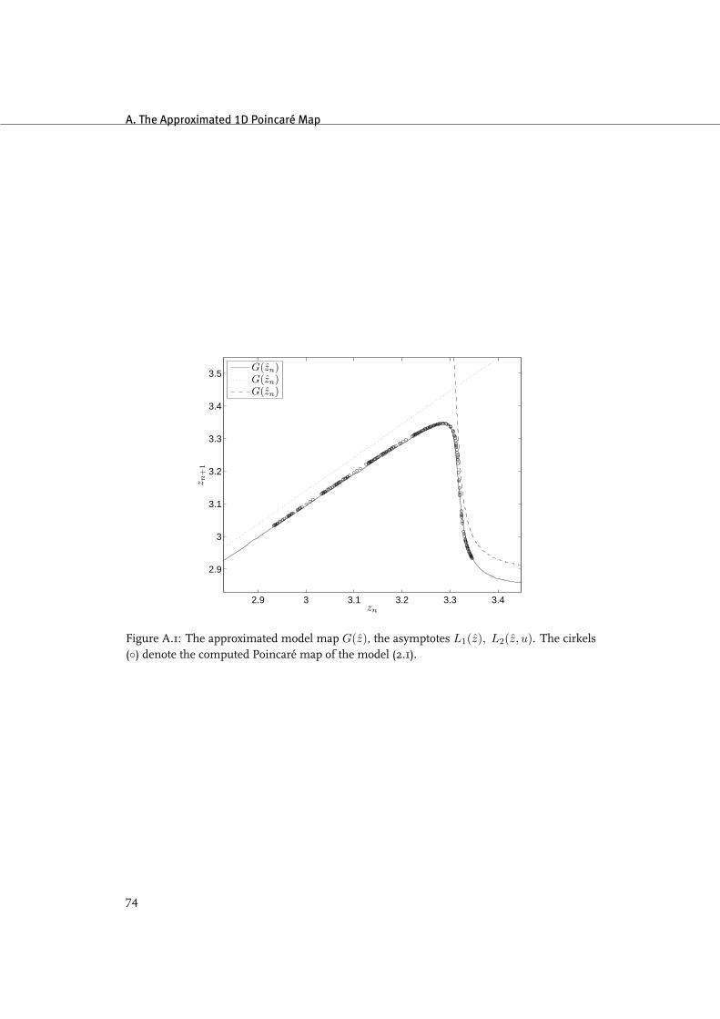
A. The Approximated 1D Poincaré Map
2.9 3 3.1 3.2 3.3 3.4
2.9
3
3.1
3.2
3.3
3.4
3.5
zn
z n+
1
G(zn)G(zn)G(zn)
Figure A.1: The approximated model map G(z), the asymptotes L1(z), L2(z, u). The cirkels() denote the computed Poincaré map of the model (2.1).
74

Appendix B
Proof of Propositions
For convenience, we recall the Hindmarsh-Rose equations:
xi = −ax3i + bx2
i + ϕ1xi + ϕ2 + gyyi − gzzi + αI + ui,
yi = −c− dx2i − ϕ3xi − βyi,
zi = r (s (xi + x0)− zi) ,
(B.1)
and the nominal parameters which are given in Table B.1
Table B.1: Hindmarsh-Rose parameter values
a = 1, b = 0, ϕ1 = 3, ϕ2 = 2, gy = 5, gz = 1, α = 1,c = 0.8, d = 1, ϕ3 = 2, β = 1, r = 0.005, s = 4, x0 = 2.6180
B.1 Proof of Proposition 4.2.2
Each system (B.1) is semi-passive. Consider the radially unbounded storage function V : R3 →R
V (x, y, z) =12cxx2 + cyy2 + czz
2
. (B.2)
The derivative of (B.2) is given by
V (x, y, z) = cxxx + cyyy + czzz
= cx
(−ax4 + bx3 + ϕ1x
2 + ϕ2x + gyxy − gzxz + αIx + ux)+
= cy
(−cy − dx2y − ϕ3xy − βy2
)+
= cz (r (s (x + x0)− z) z) .
Let y = x and cy = cxgy
ϕ3, cz = cx
gz
rs , then it is easy to verify the semi-passivity condition
V (x, y, z) ≤ yT u−H(x, y, z)
is satisfied with
H(x, y, z) = cx
(ax4 − bx3 − ϕ1x
2 − ϕ2x− αIx)+
cy
(cy + dx2y + βy2
)+ cz
(−rsx0z + rz2
).
75
B. Proof of Propositions
For the model parameters denoted in Table B.1 and cx = 1, cy = 52 and cz = 50, H(x, y, z) is
given by
H(x, y, z) = x4 − 3x2 − 2x− Ix + 2 +52x2y +
52y2 − 2.6180z +
z2
4.
B.2 Proof of Proposition 4.2.4
An analytical expression for the coupling that is required for global synchronization is derivedvia a Lyapunov function argument. Let x = x1 − x2, y = y1 − y2 and z = z1 − z2, then giventhe systems (B.1), i = 1, 2 being interconnected via the coupling functions u1 = −k(x1− x2),u2 = −k(x2 − x1) the error in the states of the systems can be written as:
˙x = −a(x3
1 − x32
)+ b
(x2
1 − x22
)+ ϕ1x + gy y − gz z − 2kx,
˙y = −d(x21 − x2
2)− ϕ3x− βy,˙z = r (sx− z) .
(B.3)
Consider the following Lyapunov function V : R3 → R
V (x) =12Cxx2 + Cy y2 + Cz z
2
, (B.4)
where x = [x, y, z]T and nonnegative constants Cx, Cy, Cz . Setting Cz = gz
rsCx, the timederivative of (B.4) is given by
V (x) = Cxx ˙x + Cy y ˙y + Cx1rs z ˙z
= Cx
−ax
(x3
1 − x32
)+ bx
(x2
1 − x22
)+ ϕ1x
2 + gy yx− gz zx− 2kx2
+ Cy
−dy
(x2
1 − x22
)− ϕ3xy − βy2
+ gz
rsCx
r(sxz − z2
)= − Cxx2
12a(x1 − b
a
)2+ 1
2a (x1 + x2)2 + 1
2a(x2 − b
a
)2 − b2
a − ϕ1 + 2k
− gz
s Cxz2 + (Cxgy − Cyϕ3)xy − Cyd(x1 + x2)xy − Cyβy2︸ ︷︷ ︸ .
(B.5)
Consider the underbraced term in (B.5). It can be written as
(Cxgy − Cyϕ3)xy − Cyd(x1 + x2)xy − Cyβy2
= 14λ1Cy
(Cxgy − Cyϕ3)2x2 −
(1
2√
λ1Cy
(Cxgy − Cyϕ3) x−√
λ1Cy y
)2
+ Cy
4λ2d2 (x1 + x2)
2x2 −
(1
2√
λ2
√Cyd (x1 + x2) x +
√Cyλ2y
)2
− Cy (β − λ1 − λ2) y2,
(B.6)
76

B.3 Proof of Proposition 4.4.1
for some λ1, λ2 > 0, λ1 + λ2 < β. Setting Cy = 2aλ2d2 Cx and substitution of (B.6) in (B.5)
yields
V (x) = −Cxx2
12a(x1 − b
a
)2+ 1
2a(x2 − b
a
)2− x2
Cx
(2k − b2
a − ϕ1
)− 1
4λ1Cy(Cxgy − Cyϕ3)
2
−(
1
2√
λ1Cy
(Cxgy − Cyϕ3) x−√
λ1Cy y
)2
−(
12√
λ2
√Cyd (x1 + x2) x +
√Cyλ2y
)2
− Cy (β − λ1 − λ2) y2 − gzCx
s z2.
The function V (·) is negative definite for
k >12
b2
a+ ϕ1 +
d2
8aλ1λ2
(gy −
2aλ2
d2ϕ3
)2
.
Therefore, for
k > kmin = minλ1,λ2>0, λ1+λ2<β
12
b2
a+ ϕ1 +
d2
8aλ1λ2
(gy −
2aλ2
d2ϕ3
)2
the system (B.3) is asymptotically stable and thus
limt→∞
‖ x ‖= 0,
limt→∞
‖ y ‖= 0,
limt→∞
‖ z ‖= 0.
B.3 Proof of Proposition 4.4.1
Consider (B.3) with noise and parameter uncertainties
˙x = −a(x3
1 − x32
)+ b
(x2
1 − x22
)+ ϕ1x + gy y − gz z − 2kx + 2kνx(t) + σx(t),
˙y = −d(x21 − x2
2)− ϕ3x− βy + σy(t),˙z = r (sx− z) + σz(t).
(B.7)
The following theorem will be used to derive the bounds on the synchronization error:
Theorem B.3.1. (Khalil, 2002) Consider the system
x = f(t,x). (B.8)
Let D ⊂ Rn be a domain that contains the origin of (B.8) and V : [0, ∞) × Rn → R be acontinuously differentiable function such that
α1(‖ x ‖) ≤ V (t,x) ≤ α2(‖ x ‖),
∂V
∂t+
∂V
∂xf(t,x) ≤ −W (x), ∀ ‖ x ‖≥ µ,
77
B. Proof of Propositions
∀ t ≥ 0 and ∀ x ⊂ D, where α1 and α2 are class-K functions and W (x) is a continuous positivedefinite function. Take r > 0 such that Br ⊂ D and suppose that
µ < α−12 α1(r).
Then, there exists a class-KL function β1 and for every initial state x(t0), satisfying ‖ x(t0) ‖≤α−1
1 α2(µ), there is T ≥ t0 (dependent on x(t0) and µ) such that the solution of (B.8) satisfies
‖ x(t) ‖≤ β1(‖ x(t0) ‖, t− t0), ∀ t0 ≤ t ≤ T, (B.9)
‖ x(t) ‖≤ α−11 α2(µ), ∀ t ≥ T. (B.10)
Moreover, if D = Rn and α1 belongs to class-K∞, then (B.9) and (B.10) hold for any initial statex(t0), with no restriction on how large µ is.
Consider the function
V (x) =12Cxx2 + Cy y2 + Cz z
2
,
eeq and its time derivative
V (x) = −Cxx2
12a(x1 − b
a
)2+ 1
2a(x2 − b
a
)2− x2
Cx
(2k − b2
a − ϕ1
)− 1
4λ1Cy(Cxgy − Cyϕ3)
2
−(
1
2√
λ1Cy
(Cxgy − Cyϕ3) x−√
λ1Cy y
)2
−(
12√
λ2
√Cyd (x1 + x2) x +
√Cyλ2y
)2
− Cy (β − λ1 − λ2) y2 − gzCx
s z2
+Cxσx(t)x + Cyσy(t)y + Cxgz
rsσz(t)z + 2kCxνx(t)x.
Introduce the continuous positive definite function W : R3 → R satisfying
V (x) ≤ −W (x), ∀ ‖ x ‖≥ µ,
for a nonnegative number µ. A possible function W (·) is
W (x) = x2
Cx
(2k − b2
a − ϕ1 − d2
8aλ1λ2
(gy − 2aλ2
d2 ϕ3
)2)+ Cx
2aλ2d2 (β − λ1 − λ2) y2 + gz
Cx
s z2
−Cx ‖ σx(t) + 2kνx(t) ‖∞ x− Cx2aλ2d2 ‖ σy(t) ‖∞ y − Cx
gz
rs ‖ σz(t) ‖∞ z.
Assume k ≥ kmin and let the following inequality hold
W (x) ≥ Cxc1 ‖ x ‖2 −Cxc2 ‖ x ‖≥ Cx (1− Ξ) c1 ‖ x ‖2, ∀ ‖ x ‖≥ c2
c1Ξ,
for some Ξ ∈ (0, 1) and
c1 = min
(2k − b2
a− ϕ1 −
d2
8aλ1λ2
(gy −
2aλ2
d2ϕ3
)2)
,
(2aλ2
d2(β − λ1 − λ2)
),(gz
s
),
c2 = max
(‖ σx(t) + 2kνx(t) ‖∞) ,
(2aλ2
d2‖ σy(t) ‖∞
),(gz
rs‖ σz(t) ‖∞
). (B.11)
78

B.3 Proof of Proposition 4.4.1
Let Cx ≤ Cy < Cxgz
rs and choose
α1(‖ x ‖) =12Cx ‖ x ‖2, α2(‖ x ‖) =
12Cx
gz
rs‖ x ‖2,
then, following Theorem B.3.1, for all initial conditions x(t0) all solutions of (B.7) are bounded
‖ x(t) ‖≤√
gz
rs
c2
c1Ξ,
for Ξ ∈ (0, 1) and c1, c2 as defined in (B.11).
79

B. Proof of Propositions
80

Appendix C
Electrical circuits
C.1 The electromechanical Hindmarsh-Rose neuron
Here the design of the electromechanical Hindmarsh-Rose neuron is discussed using somebasic electrical circuits.
An important part of the electromechanical neuron are the integrator circuits. These cir-cuits integrate the three differential equations (2.1). A single integrator circuit is depictedin Figure C.1. Applying the well known proporties of operational amplifiers and Kirchhoff’slaws, one can easily see that this circuit can be described by the equation
CVout +1
R1Vin,1 +
1R2
Vin,2 + . . . +1
RnVin,n = 0,
or
Vout = − 1R1C
Vin,1 −1
R2CVin,2 − . . .− 1
RnCVin,n.
It follows immediately that the equations (3.1) correspond to the circuits depicted in Figure3.1.
Vout
1MΩ 1MΩ
C
R1
R2
+
−Vin,1
Vin,2
Rn
Vin,n
Figure C.1: Integrating circuit
As showed in Figure 3.1 the sign of some signals has to he changed, e.g. −x and −y.Therefore, inverting circuits are used. The inverting circuit consist of a operational amplifier
81
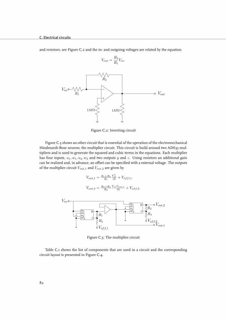
C. Electrical circuits
and resistors, see Figure C.2 and the in- and outgoing voltages are related by the equation
Vout =R2
R1Vin.
Vout
1MΩ 1MΩ
R2
R1
+
−Vin
Figure C.2: Inverting circuit
Figure C.3 shows an other circuit that is essential of the operation of the electromechanicalHindmarsh-Rose neuron; the multiplier circuit. This circuit is build around two AD633 mul-tipliers and is used to generate the squared and cubic terms in the equations. Each multiplierhas four inputs, u1, w1, u2, w2 and two outputs y and z. Using resistors an additional gaincan be realized and, in advance, an offset can be specified with a external voltage. The outputsof the multiplier circuit Vout,1 and Vout,2 are given by
Vout,1 = R1+R2R1
V 2in
10 + Voff,1,
Vout,2 = R3+R4R3
VinVout,110 + Voff,2.
R1
R2
Vin
u1w1u2w2
y
z
u1w1u2w2
y
zR3
R4
Vout,2
Vout,1Voff,1
Voff,2
Figure C.3: The multiplier circuit
Table C.1 shows the list of components that are used in a circuit and the correspondingcircuit layout is presented in Figure C.4.
82
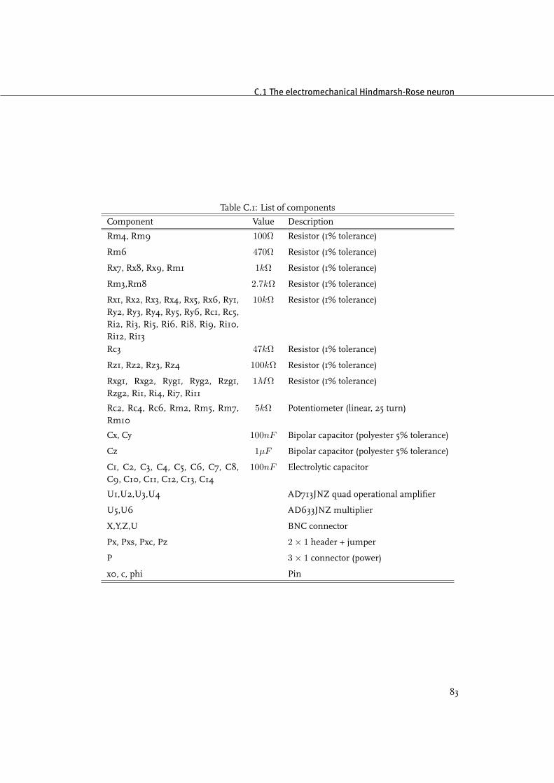
C.1 The electromechanical Hindmarsh-Rose neuron
Table C.1: List of components
Component Value Description
Rm4, Rm9 100Ω Resistor (1% tolerance)
Rm6 470Ω Resistor (1% tolerance)
Rx7, Rx8, Rx9, Rm1 1kΩ Resistor (1% tolerance)
Rm3,Rm8 2.7kΩ Resistor (1% tolerance)
Rx1, Rx2, Rx3, Rx4, Rx5, Rx6, Ry1,Ry2, Ry3, Ry4, Ry5, Ry6, Rc1, Rc5,Ri2, Ri3, Ri5, Ri6, Ri8, Ri9, Ri10,Ri12, Ri13
10kΩ Resistor (1% tolerance)
Rc3 47kΩ Resistor (1% tolerance)
Rz1, Rz2, Rz3, Rz4 100kΩ Resistor (1% tolerance)
Rxg1, Rxg2, Ryg1, Ryg2, Rzg1,Rzg2, Ri1, Ri4, Ri7, Ri11
1MΩ Resistor (1% tolerance)
Rc2, Rc4, Rc6, Rm2, Rm5, Rm7,Rm10
5kΩ Potentiometer (linear, 25 turn)
Cx, Cy 100nF Bipolar capacitor (polyester 5% tolerance)
Cz 1µF Bipolar capacitor (polyester 5% tolerance)
C1, C2, C3, C4, C5, C6, C7, C8,C9, C10, C11, C12, C13, C14
100nF Electrolytic capacitor
U1,U2,U3,U4 AD713JNZ quad operational amplifier
U5,U6 AD633JNZ multiplier
X,Y,Z,U BNC connector
Px, Pxs, Pxc, Pz 2× 1 header + jumper
P 3× 1 connector (power)
x0, c, phi Pin
83

C. Electrical circuits0 0
1 1
2 2
3 3
4 4
5 5
6 6
7 7
8 8
9 9
10
10
11
11
12
12
13
13
14
14
AA
BB
CC
DD
EE
FF
GG
HH
II
JJ
Rz3
Rz4
Ri1
3
Ri1
0
Ri6
Ri3
Ri2
Ri5
Ri8
Ri1
2
Ri9
Rz1
Rz2
Rc1
Y
Z
X
Cz
C1
C2
Rc5
U
U5
U6
Rm
1
Rm
6
Rm
3
Rm
8
ph
i
cx0
P
Pz
Px Pxs
Pxc
Ryg
1
Ryg
2
Rzg
1
Rzg
2
Rxg
2
Rxg
1R
i1
Ri4
Ri7
Ri1
1
Cx
Cy
Rx1
Rx2
Rx3
Rx4
Rx5
Rx6
Rx7
Rx8
Rx9
Ry1
Ry2
Ry3
Ry4
Ry5
Ry6
C3
C5
C7
C9
C1
0
C8
C6
C4
C1
3
C1
4
C1
2
C11
U1
A
U1
B
U1
C
U1
D
U2
A
U2
B
U2
C
U2
D
U3
A
U3
B
U3
C
U3
D
U4
A
U4
B
U4
C
U4
D
Rc3
Rm
4
Rm
7
Rm
10
Rm
9
Rm
5
Rc2
Rc4
Rc6
Rm
2
Figure C.4: Circuit layout
84

C.2 Interface board
Signal reshaping Signal reshapingAD7026µC⇒ ⇒Vin,1 →
Vin,4 →Vin,3 →Vin,2 →
Vout,1→
Vout,4→Vout,3→Vout,2→
⇓u
Figure C.5: Abstract of the synchronization interface
C.2 Interface board
The synchronization interface is build around a ADuC7026 microcontroller. This controlleruses a ARM7TDMI core (16-bit/32-bit instruction set and RISC architecture) which operatesat about 42 [Mhz]. Twelve Analog-Digital Converters (ADCs) are directly available which allhave a 12-bit resolution over the range 0−2.5 [V ]. In addition, the microcontroller has four 12-bit Digital-Analog Converters (DACs) that, again, cover the range 0−2.5 [V ]. These convertersare fast enough such that the time delay that is caused by the conversion in negligibly small.A delay of maximal ≈ 1 · 10−5 [s] is measured.
Because the signals that are generated by each individual circuit and the outputs of thecouplings functions are outside the range of both the ADCs and the DACs, some signalsreshaping has to take place. Figure C.5 shows the synchronization interface schematically.
85

C. Electrical circuits
86
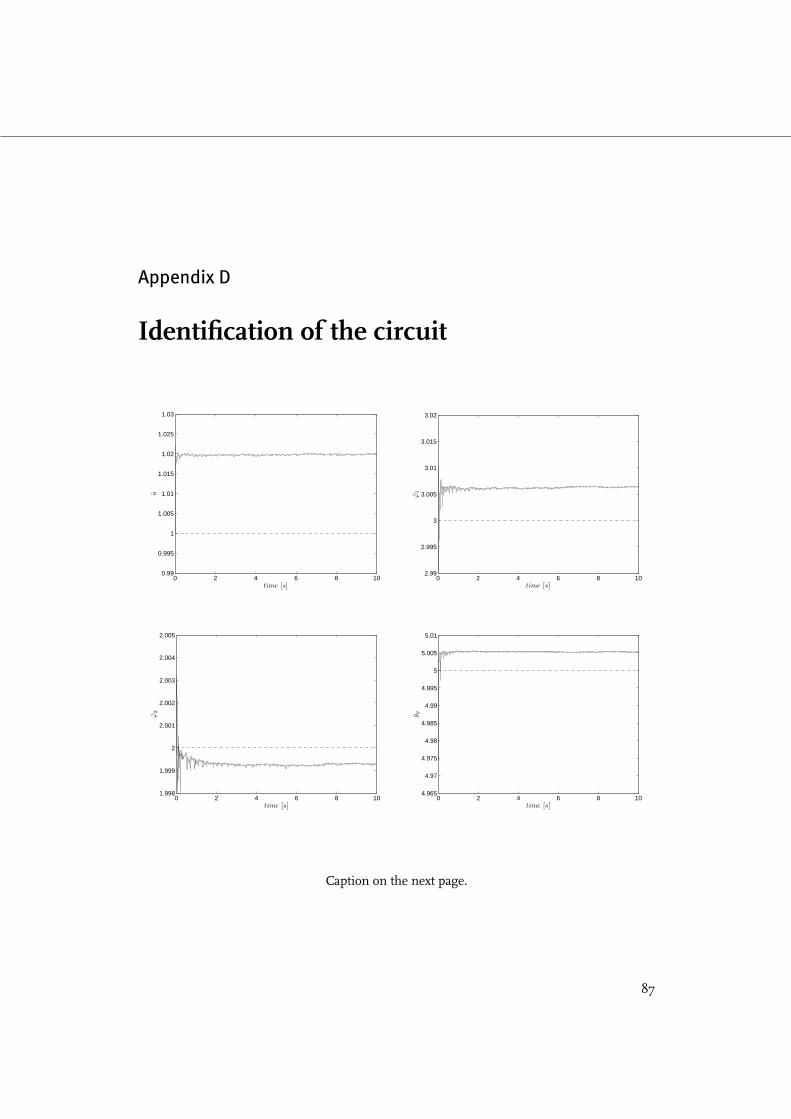
Appendix D
Identification of the circuit
0 2 4 6 8 100.99
0.995
1
1.005
1.01
1.015
1.02
1.025
1.03
time [s]
a
0 2 4 6 8 102.99
2.995
3
3.005
3.01
3.015
3.02
time [s]
ϕ1
0 2 4 6 8 101.998
1.999
2
2.001
2.002
2.003
2.004
2.005
time [s]
ϕ2
0 2 4 6 8 104.965
4.97
4.975
4.98
4.985
4.99
4.995
5
5.005
5.01
time [s]
g y
Caption on the next page.
87

D. Identification of the circuit
0 2 4 6 8 100.985
0.99
0.995
1
1.005
1.01
time [s]
g z
0 2 4 6 8 100.99
0.995
1
1.005
1.01
1.015
time [s]α
0 2 4 6 8 100.73
0.74
0.75
0.76
0.77
0.78
0.79
0.8
0.81
time [s]
c
0 2 4 6 8 100.99
0.995
1
1.005
1.01
1.015
1.02
time [s]
d
0 2 4 6 8 101.97
1.98
1.99
2
2.01
2.02
2.03
time [s]
ϕ3
0 2 4 6 8 100.98
0.985
0.99
0.995
1
1.005
time [s]
β
Figure D.1: The parameter estimations.
88
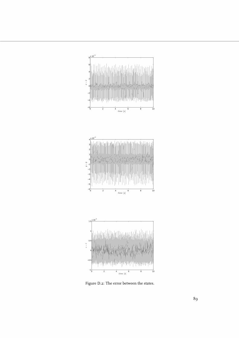
0 2 4 6 8 10−6
−4
−2
0
2
4
6
8x 10
−3
time [s]
x−
x
0 2 4 6 8 10−6
−5
−4
−3
−2
−1
0
1
2
3
4x 10
−3
time [s]
y−
y
0 2 4 6 8 10−1
−0.5
0
0.5
1
1.5x 10
−3
time [s]
z−
z
Figure D.2: The error between the states.
89

D. Identification of the circuit
90
Appendix E
Additional measurements
In this appendix extra plots of a single circuit and the synchronous state are showed.
E.1 Single circuit
E.1.1 Constant inputs
0 0.2 0.4 0.6 0.8 1−3
−2
−1
0
1
time [s]
x[V
]
0 0.2 0.4 0.6 0.8 1−3
−2
−1
0
time [s]
y[V
]
0 0.2 0.4 0.6 0.8 1
1.4
1.6
1.8
time [s]
z[V
]
(a) u = 1.5
0 0.2 0.4 0.6 0.8 1−3
−2
−1
0
1
time [s]
x[V
]
0 0.2 0.4 0.6 0.8 1
−2
−1
0
time [s]
y[V
]
0 0.2 0.4 0.6 0.8 1
1.6
1.8
2
time [s]
z[V
]
(b) u = 1.75
0 0.2 0.4 0.6 0.8 1−3
−2
−1
0
1
time [s]
x[V
]
0 0.2 0.4 0.6 0.8 1−3
−2
−1
0
time [s]
y[V
]
0 0.2 0.4 0.6 0.8 1
1.8
2
2.2
2.4
time [s]
z[V
]
(c) u = 2
0 0.2 0.4 0.6 0.8 1−3
−2
−1
0
1
time [s]
x[V
]
0 0.2 0.4 0.6 0.8 1
−2
−1
0
time [s]
y[V
]
0 0.2 0.4 0.6 0.8 1
2
2.2
2.4
time [s]
z[V
]
(d) u = 2.25
91
E. Additional measurements
0 0.2 0.4 0.6 0.8 1−3
−2
−1
0
1
time [s]
x[V
]
0 0.2 0.4 0.6 0.8 1
−2
−1
0
time [s]
y[V
]
0 0.2 0.4 0.6 0.8 12.2
2.4
2.6
2.8
time [s]
z[V
]
(e) u = 2.5
0 0.2 0.4 0.6 0.8 1−3
−2
−1
0
1
time [s]
x[V
]
0 0.2 0.4 0.6 0.8 1
−2
−1
0
time [s]
y[V
]
0 0.2 0.4 0.6 0.8 1
2.6
2.8
3
time [s]
z[V
]
(f) u = 2.75
0 0.2 0.4 0.6 0.8 1−3
−2
−1
0
1
time [s]
x[V
]
0 0.2 0.4 0.6 0.8 1
−2
−1
0
time [s]
y[V
]
0 0.2 0.4 0.6 0.8 12.6
2.8
3
3.2
time [s]
z[V
]
(g) u = 3
0 0.2 0.4 0.6 0.8 1
−2
−1
0
1
time [s]
x[V
]
0 0.2 0.4 0.6 0.8 1−2
−1
0
time [s]
y[V
]
0 0.2 0.4 0.6 0.8 1
3
3.2
3.4
time [s]
z[V
]
(h) u = 3.25
0 0.2 0.4 0.6 0.8 1
−2
−1
0
1
time [s]
x[V
]
0 0.2 0.4 0.6 0.8 1−1.5
−1
−0.5
0
0.5
time [s]
y[V
]
0 0.2 0.4 0.6 0.8 13.5
3.6
3.7
3.8
time [s]
z[V
]
(i) u = 3.5
0 0.2 0.4 0.6 0.8 1
−2
−1
0
1
time [s]
x[V
]
0 0.2 0.4 0.6 0.8 1−1.5
−1
−0.5
0
0.5
time [s]
y[V
]
0 0.2 0.4 0.6 0.8 13.8
3.9
4
time [s]
z[V
]
(j) u = 3.75
92
E.1 Single circuit
0 0.2 0.4 0.6 0.8 1
−2
−1
0
1
time [s]
x[V
]
0 0.2 0.4 0.6 0.8 1−1.5
−1
−0.5
0
0.5
time [s]
y[V
]
0 0.2 0.4 0.6 0.8 14
4.1
4.2
time [s]
z[V
]
(k) u = 4
0 0.2 0.4 0.6 0.8 1
−2
−1
0
1
time [s]
x[V
]
0 0.2 0.4 0.6 0.8 1−1.5
−1
−0.5
0
0.5
time [s]
y[V
]0 0.2 0.4 0.6 0.8 1
4.2
4.3
4.4
time [s]z
[V]
(l) u = 4.25
0 0.2 0.4 0.6 0.8 1
−2
−1
0
1
time [s]
x[V
]
0 0.2 0.4 0.6 0.8 1−1.5
−1
−0.5
0
0.5
time [s]
y[V
]
0 0.2 0.4 0.6 0.8 14.4
4.5
4.6
time [s]
z[V
]
(m) u = 4.5
0 0.2 0.4 0.6 0.8 1
−2
−1
0
1
time [s]
x[V
]
0 0.2 0.4 0.6 0.8 1
−1.5−1
−0.50
0.5
time [s]
y[V
]
0 0.2 0.4 0.6 0.8 14.6
4.7
4.8
time [s]
z[V
]
(n) u = 4.75
0 0.2 0.4 0.6 0.8 1
−2
−1
0
1
time [s]
x[V
]
0 0.2 0.4 0.6 0.8 1
−1.5−1
−0.50
0.5
time [s]
y[V
]
0 0.2 0.4 0.6 0.8 1
4.824.844.864.884.9
time [s]
z[V
]
(o) u = 5
Figure E.1: Circuit responses on constant inputs u.
93
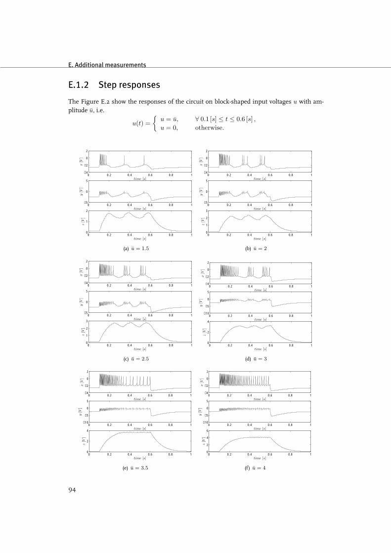
E. Additional measurements
E.1.2 Step responses
The Figure E.2 show the responses of the circuit on block-shaped input voltages u with am-plitude u, i.e.
u(t) =
u = u, ∀ 0.1 [s] ≤ t ≤ 0.6 [s] ,u = 0, otherwise.
0 0.2 0.4 0.6 0.8 1−4
−2
0
2
time [s]
x[V
]
0 0.2 0.4 0.6 0.8 1−5
0
5
time [s]
y[V
]
0 0.2 0.4 0.6 0.8 10
1
2
time [s]
z[V
]
(a) u = 1.5
0 0.2 0.4 0.6 0.8 1−4
−2
0
2
time [s]
x[V
]
0 0.2 0.4 0.6 0.8 1−5
0
5
time [s]
y[V
]
0 0.2 0.4 0.6 0.8 10
1
2
3
time [s]
z[V
]
(b) u = 2
0 0.2 0.4 0.6 0.8 1−4
−2
0
2
time [s]
x[V
]
0 0.2 0.4 0.6 0.8 1−5
0
5
time [s]
y[V
]
0 0.2 0.4 0.6 0.8 10
1
2
3
time [s]
z[V
]
(c) u = 2.5
0 0.2 0.4 0.6 0.8 1−4
−2
0
2
time [s]
x[V
]
0 0.2 0.4 0.6 0.8 1−10
−5
0
5
time [s]
y[V
]
0 0.2 0.4 0.6 0.8 10
2
4
time [s]
z[V
]
(d) u = 3
0 0.2 0.4 0.6 0.8 1−4
−2
0
2
time [s]
x[V
]
0 0.2 0.4 0.6 0.8 1−10
−5
0
5
time [s]
y[V
]
0 0.2 0.4 0.6 0.8 10
2
4
time [s]
z[V
]
(e) u = 3.5
0 0.2 0.4 0.6 0.8 1−4
−2
0
2
time [s]
x[V
]
0 0.2 0.4 0.6 0.8 1−10
−5
0
5
time [s]
y[V
]
0 0.2 0.4 0.6 0.8 10
2
4
6
time [s]
z[V
]
(f) u = 4
94
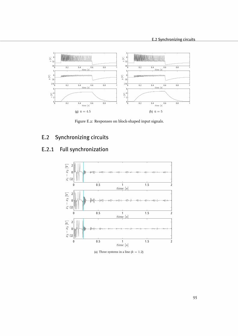
E.2 Synchronizing circuits
0 0.2 0.4 0.6 0.8 1−4
−2
0
2
time [s]
x[V
]
0 0.2 0.4 0.6 0.8 1−10
−5
0
5
time [s]
y[V
]
0 0.2 0.4 0.6 0.8 10
2
4
6
time [s]
z[V
]
(g) u = 4.5
0 0.2 0.4 0.6 0.8 1−4
−2
0
2
time [s]
x[V
]
0 0.2 0.4 0.6 0.8 1−10
−5
0
5
time [s]
y[V
]
0 0.2 0.4 0.6 0.8 10
2
4
6
time [s]
z[V
]
(h) u = 5
Figure E.2: Responses on block-shaped input signals.
E.2 Synchronizing circuits
E.2.1 Full synchronization
0 0.5 1 1.5 2
−2
0
2
time [s]
x1−
x2
[V]
0 0.5 1 1.5 2
−2
0
2
time [s]
x1−
x3
[V]
0 0.5 1 1.5 2
−2
0
2
time [s]
x2−
x3
[V]
(a) Three systems in a line (k = 1.2)
95
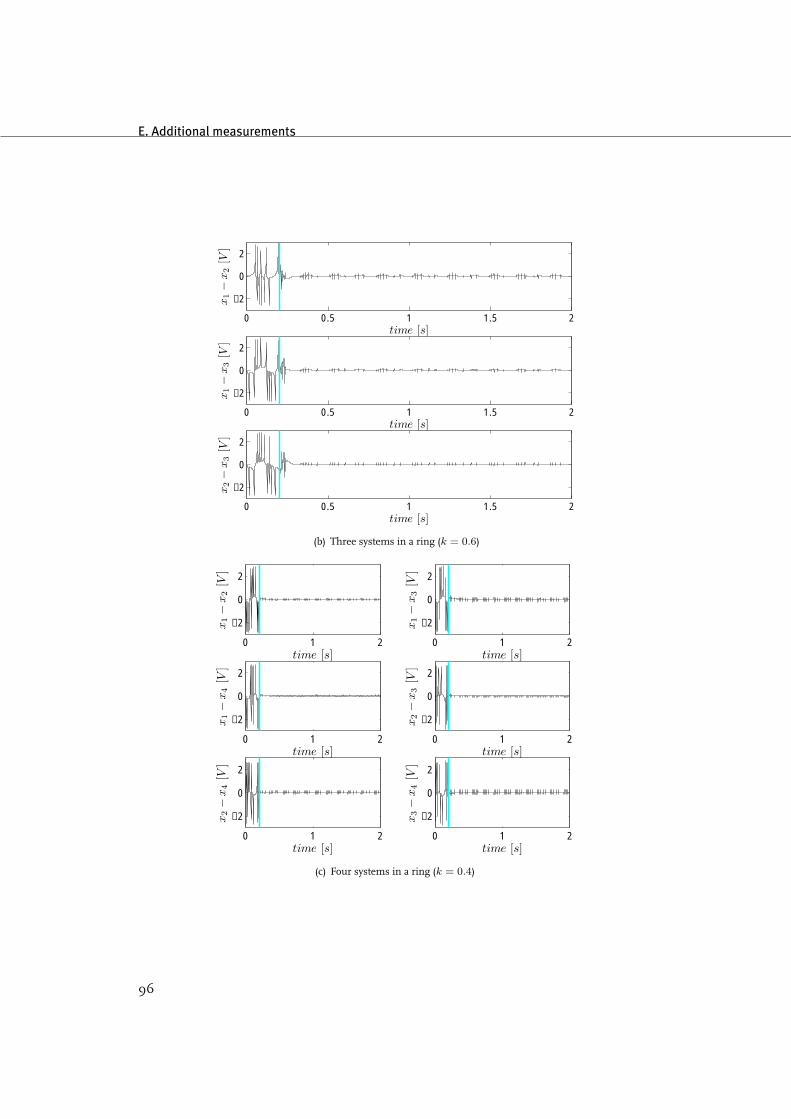
E. Additional measurements
0 0.5 1 1.5 2
−2
0
2
time [s]
x1−
x2
[V]
0 0.5 1 1.5 2
−2
0
2
time [s]
x1−
x3
[V]
0 0.5 1 1.5 2
−2
0
2
time [s]
x2−
x3
[V]
(b) Three systems in a ring (k = 0.6)
0 1 2
−2
0
2
time [s]
x1−
x2
[V]
0 1 2
−2
0
2
time [s]
x1−
x3
[V]
0 1 2
−2
0
2
time [s]
x1−
x4
[V]
0 1 2
−2
0
2
time [s]
x2−
x3
[V]
0 1 2
−2
0
2
time [s]
x2−
x4
[V]
0 1 2
−2
0
2
time [s]
x3−
x4
[V]
(c) Four systems in a ring (k = 0.4)
96
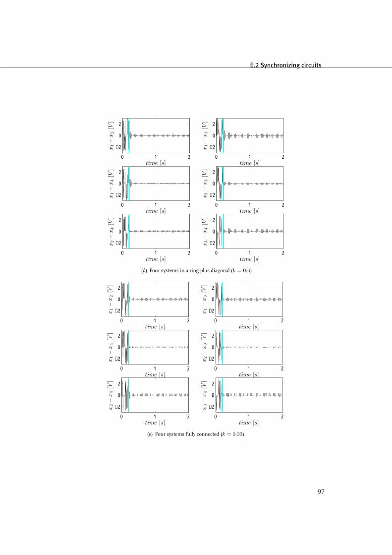
E.2 Synchronizing circuits
0 1 2
−2
0
2
time [s]
x1−
x2
[V]
0 1 2
−2
0
2
time [s]
x1−
x3
[V]
0 1 2
−2
0
2
time [s]
x1−
x4
[V]
0 1 2
−2
0
2
time [s]x
2−
x3
[V]
0 1 2
−2
0
2
time [s]
x2−
x4
[V]
0 1 2
−2
0
2
time [s]
x3−
x4
[V]
(d) Four systems in a ring plus diagonal (k = 0.6)
0 1 2
−2
0
2
time [s]
x1−
x2
[V]
0 1 2
−2
0
2
time [s]
x1−
x3
[V]
0 1 2
−2
0
2
time [s]
x1−
x4
[V]
0 1 2
−2
0
2
time [s]
x2−
x3
[V]
0 1 2
−2
0
2
time [s]
x2−
x4
[V]
0 1 2
−2
0
2
time [s]
x3−
x4
[V]
(e) Four systems fully connected (k = 0.33)
97

E. Additional measurements
0 1 2
−2
0
2
time [s]
x1−
x2
[V]
0 1 2
−2
0
2
time [s]
x1−
x3
[V]
0 1 2
−2
0
2
time [s]
x1−
x4
[V]
0 1 2
−2
0
2
time [s]x
2−
x3
[V]
0 1 2
−2
0
2
time [s]
x2−
x4
[V]
0 1 2
−2
0
2
time [s]
x3−
x4
[V]
(f) Four systems in the network of Example 4.5.1 (k = 1.1)
0 1 2
−2
0
2
time [s]
x1−
x2
[V]
0 1 2
−2
0
2
time [s]
x1−
x3
[V]
0 1 2
−2
0
2
time [s]
x1−
x4
[V]
0 1 2
−2
0
2
time [s]
x2−
x3
[V]
0 1 2
−2
0
2
time [s]
x2−
x4
[V]
0 1 2
−2
0
2
time [s]
x3−
x4
[V]
(g) Four systems in a line (k = 2.2)
Figure E.3: Full synchronization
98
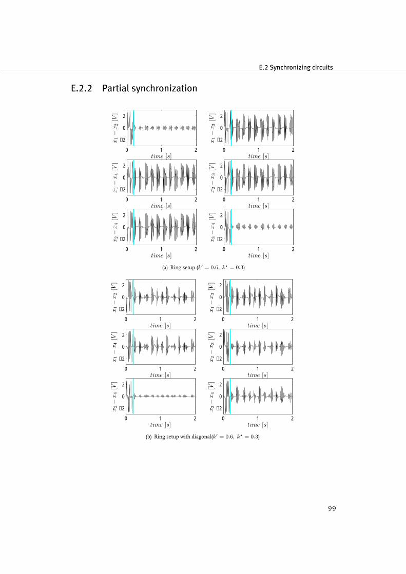
E.2 Synchronizing circuits
E.2.2 Partial synchronization
0 1 2
−2
0
2
time [s]
x1−
x2
[V]
0 1 2
−2
0
2
time [s]
x1−
x3
[V]
0 1 2
−2
0
2
time [s]
x1−
x4
[V]
0 1 2
−2
0
2
time [s]x
2−
x3
[V]
0 1 2
−2
0
2
time [s]
x2−
x4
[V]
0 1 2
−2
0
2
time [s]
x3−
x4
[V]
(a) Ring setup (k′ = 0.6, k? = 0.3)
0 1 2
−2
0
2
time [s]
x1−
x2
[V]
0 1 2
−2
0
2
time [s]
x1−
x3
[V]
0 1 2
−2
0
2
time [s]
x1−
x4
[V]
0 1 2
−2
0
2
time [s]
x2−
x3
[V]
0 1 2
−2
0
2
time [s]
x2−
x4
[V]
0 1 2
−2
0
2
time [s]
x3−
x4
[V]
(b) Ring setup with diagonal(k′ = 0.6, k? = 0.3)
99
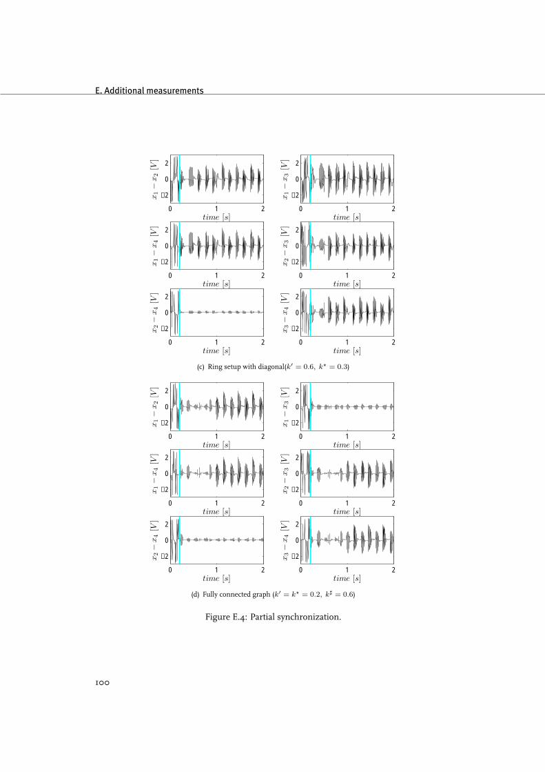
E. Additional measurements
0 1 2
−2
0
2
time [s]
x1−
x2
[V]
0 1 2
−2
0
2
time [s]
x1−
x3
[V]
0 1 2
−2
0
2
time [s]
x1−
x4
[V]
0 1 2
−2
0
2
time [s]x
2−
x3
[V]
0 1 2
−2
0
2
time [s]
x2−
x4
[V]
0 1 2
−2
0
2
time [s]
x3−
x4
[V]
(c) Ring setup with diagonal(k′ = 0.6, k? = 0.3)
0 1 2
−2
0
2
time [s]
x1−
x2
[V]
0 1 2
−2
0
2
time [s]
x1−
x3
[V]
0 1 2
−2
0
2
time [s]
x1−
x4
[V]
0 1 2
−2
0
2
time [s]
x2−
x3
[V]
0 1 2
−2
0
2
time [s]
x2−
x4
[V]
0 1 2
−2
0
2
time [s]
x3−
x4
[V]
(d) Fully connected graph (k′ = k? = 0.2, k] = 0.6)
Figure E.4: Partial synchronization.
100

Appendix F
Selected Papers
This appendix includes several additional publications and conference contributions that aremade in this period.
• The first two included documents show the extended abstract and the poster for theInternational Symposium on Synchronization in Complex Networks poster session contri-bution. This work is directly related to the subject of this thesis.
• The next document is PhysCon 2007 conference paper Reconstructing Dynamics of Spik-ing Neuron from Input-Output Measurements in vitro. This paper is based on previouswork that is done during the author’s internship at Riken BSI.
• The last paper Non-uniform Small-gain Theorems for Systems with Unstable Invariant Setsis accepted for the SIAM Journal on Control and Optimization. This paper deals withthe asymptotic proporties of interconnected dynamical systems.
101

F. Selected Papers
102
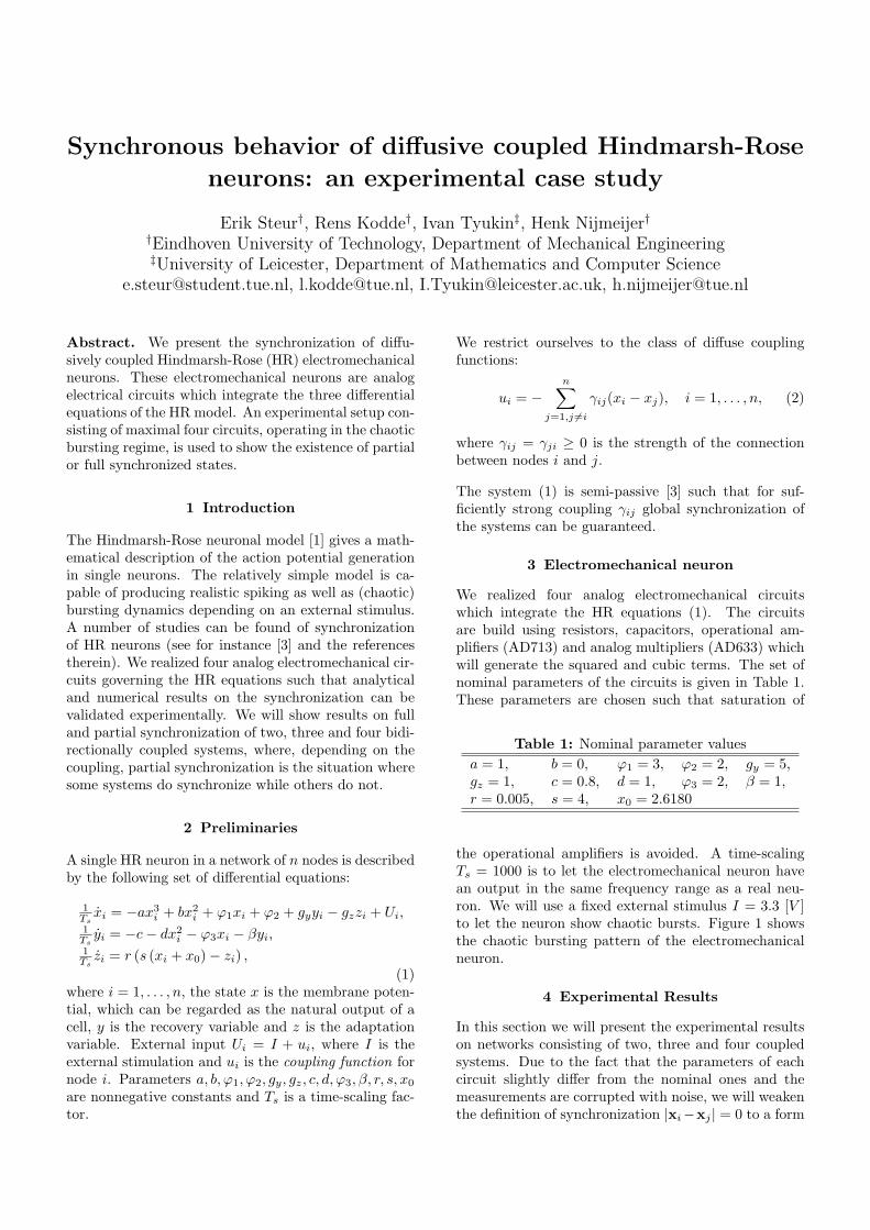
Synchronous behavior of diffusive coupled Hindmarsh-Rose
neurons: an experimental case study
Erik Steur†, Rens Kodde†, Ivan Tyukin‡, Henk Nijmeijer††Eindhoven University of Technology, Department of Mechanical Engineering‡University of Leicester, Department of Mathematics and Computer Science
[email protected], [email protected], [email protected], [email protected]
Abstract. We present the synchronization of diffu-sively coupled Hindmarsh-Rose (HR) electromechanicalneurons. These electromechanical neurons are analogelectrical circuits which integrate the three differentialequations of the HR model. An experimental setup con-sisting of maximal four circuits, operating in the chaoticbursting regime, is used to show the existence of partialor full synchronized states.
1 Introduction
The Hindmarsh-Rose neuronal model [1] gives a math-ematical description of the action potential generationin single neurons. The relatively simple model is ca-pable of producing realistic spiking as well as (chaotic)bursting dynamics depending on an external stimulus.A number of studies can be found of synchronizationof HR neurons (see for instance [3] and the referencestherein). We realized four analog electromechanical cir-cuits governing the HR equations such that analyticaland numerical results on the synchronization can bevalidated experimentally. We will show results on fulland partial synchronization of two, three and four bidi-rectionally coupled systems, where, depending on thecoupling, partial synchronization is the situation wheresome systems do synchronize while others do not.
2 Preliminaries
A single HR neuron in a network of n nodes is describedby the following set of differential equations:
1Ts
xi = −ax3i + bx2
i + ϕ1xi + ϕ2 + gyyi − gzzi + Ui,1Ts
yi = −c− dx2i − ϕ3xi − βyi,
1Ts
zi = r (s (xi + x0)− zi) ,
(1)where i = 1, . . . , n, the state x is the membrane poten-tial, which can be regarded as the natural output of acell, y is the recovery variable and z is the adaptationvariable. External input Ui = I + ui, where I is theexternal stimulation and ui is the coupling function fornode i. Parameters a, b, ϕ1, ϕ2, gy, gz, c, d, ϕ3, β, r, s, x0
are nonnegative constants and Ts is a time-scaling fac-tor.
We restrict ourselves to the class of diffuse couplingfunctions:
ui = −n∑
j=1,j 6=i
γij(xi − xj), i = 1, . . . , n, (2)
where γij = γji ≥ 0 is the strength of the connectionbetween nodes i and j.
The system (1) is semi-passive [3] such that for suf-ficiently strong coupling γij global synchronization ofthe systems can be guaranteed.
3 Electromechanical neuron
We realized four analog electromechanical circuitswhich integrate the HR equations (1). The circuitsare build using resistors, capacitors, operational am-plifiers (AD713) and analog multipliers (AD633) whichwill generate the squared and cubic terms. The set ofnominal parameters of the circuits is given in Table 1.These parameters are chosen such that saturation of
Table 1: Nominal parameter valuesa = 1, b = 0, ϕ1 = 3, ϕ2 = 2, gy = 5,gz = 1, c = 0.8, d = 1, ϕ3 = 2, β = 1,r = 0.005, s = 4, x0 = 2.6180
the operational amplifiers is avoided. A time-scalingTs = 1000 is to let the electromechanical neuron havean output in the same frequency range as a real neu-ron. We will use a fixed external stimulus I = 3.3 [V ]to let the neuron show chaotic bursts. Figure 1 showsthe chaotic bursting pattern of the electromechanicalneuron.
4 Experimental Results
In this section we will present the experimental resultson networks consisting of two, three and four coupledsystems. Due to the fact that the parameters of eachcircuit slightly differ from the nominal ones and themeasurements are corrupted with noise, we will weakenthe definition of synchronization |xi−xj | = 0 to a form
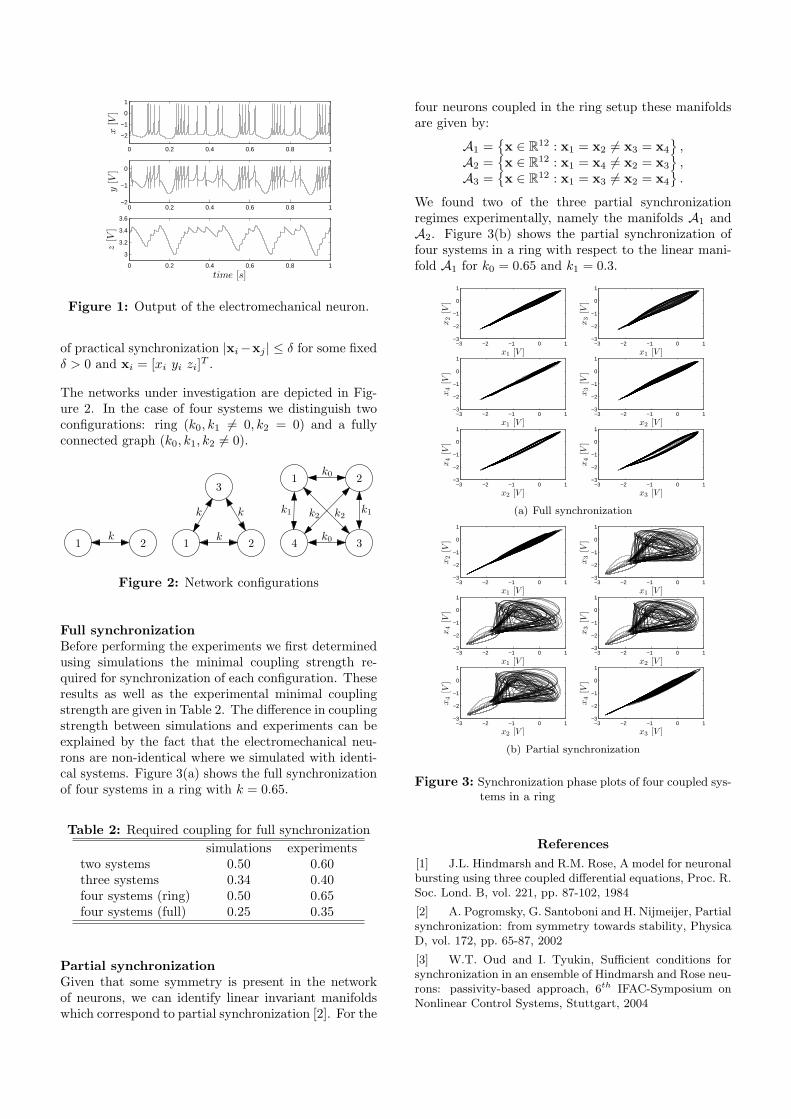
0 0.2 0.4 0.6 0.8 1
−2
−1
0
1
x[V
]
0 0.2 0.4 0.6 0.8 1−2
−1
0
y[V
]
0 0.2 0.4 0.6 0.8 1
3
3.2
3.4
3.6
time [s]
z[V
]
Figure 1: Output of the electromechanical neuron.
of practical synchronization |xi−xj | ≤ δ for some fixedδ > 0 and xi = [xi yi zi]T .
The networks under investigation are depicted in Fig-ure 2. In the case of four systems we distinguish twoconfigurations: ring (k0, k1 6= 0, k2 = 0) and a fullyconnected graph (k0, k1, k2 6= 0).
1 2k
1 2k
3
kk
1 2k0
4 3k0
k1k1 k2k2
Figure 2: Network configurations
Full synchronizationBefore performing the experiments we first determinedusing simulations the minimal coupling strength re-quired for synchronization of each configuration. Theseresults as well as the experimental minimal couplingstrength are given in Table 2. The difference in couplingstrength between simulations and experiments can beexplained by the fact that the electromechanical neu-rons are non-identical where we simulated with identi-cal systems. Figure 3(a) shows the full synchronizationof four systems in a ring with k = 0.65.
Table 2: Required coupling for full synchronizationsimulations experiments
two systems 0.50 0.60three systems 0.34 0.40four systems (ring) 0.50 0.65four systems (full) 0.25 0.35
Partial synchronizationGiven that some symmetry is present in the networkof neurons, we can identify linear invariant manifoldswhich correspond to partial synchronization [2]. For the
four neurons coupled in the ring setup these manifoldsare given by:
A1 =x ∈ R12 : x1 = x2 6= x3 = x4
,
A2 =x ∈ R12 : x1 = x4 6= x2 = x3
,
A3 =x ∈ R12 : x1 = x3 6= x2 = x4
.
We found two of the three partial synchronizationregimes experimentally, namely the manifolds A1 andA2. Figure 3(b) shows the partial synchronization offour systems in a ring with respect to the linear mani-fold A1 for k0 = 0.65 and k1 = 0.3.
−3 −2 −1 0 1−3
−2
−1
0
1
x1 [V ]
x2
[V]
−3 −2 −1 0 1−3
−2
−1
0
1
x1 [V ]
x3
[V]
−3 −2 −1 0 1−3
−2
−1
0
1
x1 [V ]
x4
[V]
−3 −2 −1 0 1−3
−2
−1
0
1
x2 [V ]
x3
[V]
−3 −2 −1 0 1−3
−2
−1
0
1
x2 [V ]
x4
[V]
−3 −2 −1 0 1−3
−2
−1
0
1
x3 [V ]
x4
[V]
(a) Full synchronization
−3 −2 −1 0 1−3
−2
−1
0
1
x1 [V ]
x2
[V]
−3 −2 −1 0 1−3
−2
−1
0
1
x1 [V ]x
3[V
]
−3 −2 −1 0 1−3
−2
−1
0
1
x1 [V ]
x4
[V]
−3 −2 −1 0 1−3
−2
−1
0
1
x2 [V ]
x3
[V]
−3 −2 −1 0 1−3
−2
−1
0
1
x2 [V ]
x4
[V]
−3 −2 −1 0 1−3
−2
−1
0
1
x3 [V ]
x4
[V]
(b) Partial synchronization
Figure 3: Synchronization phase plots of four coupled sys-tems in a ring
References[1] J.L. Hindmarsh and R.M. Rose, A model for neuronalbursting using three coupled differential equations, Proc. R.Soc. Lond. B, vol. 221, pp. 87-102, 1984
[2] A. Pogromsky, G. Santoboni and H. Nijmeijer, Partialsynchronization: from symmetry towards stability, PhysicaD, vol. 172, pp. 65-87, 2002
[3] W.T. Oud and I. Tyukin, Sufficient conditions forsynchronization in an ensemble of Hindmarsh and Rose neu-rons: passivity-based approach, 6th IFAC-Symposium onNonlinear Control Systems, Stuttgart, 2004
12
/w
Synchronous Behavior of Diffusively CoupledHindmarsh-Rose Neurons: An Experimental Case Study
Erik Steur†, Rens Kodde†, Ivan Tyukin‡, Henk Nijmeijer†
† Eindhoven University of Technology, Department of Mechanical Engineering‡ University of Leicester, Department of Mathematics and Computerscience
[email protected], [email protected], [email protected], [email protected]
IntroductionThe Hindmarsh-Rose neuronal (HR) model [1] gives a mathe-matical description of the action potential generation in sin-gle neurons. Four analog electromechanical circuits govern-ing the HR equations are realized to investigate synchroniza-tion experimentally. We present experimental results on fulland partial synchronization of four bidirectionally coupledsystems in a ring, where, depending on the coupling, par-tial synchronization is the situation where some systems dosynchronize while others do not.
Figure 1. The electromechanical Hindmarsh-Rose system.
PreliminariesThe network of four HR systems is described by:
1Ts
xi = −ax3i + bx2
i + ϕ1xi + ϕ2 + gyyi − gzzi + Ui,1Ts
yi = −c− dx2i − ϕ3xi − βyi,
1Ts
zi = r (s (xi + x0)− zi) , i = 1, . . . , 4,
(1)
where the state x is the membrane potential, which canbe regarded as the natural output of a neuron, y is therecovery variable and z is the adaptation variable. Exter-nal input Ui = I + ui, where I is the external stim-ulation and ui is the coupling function for node i. Pa-rameters a, b, ϕ1, ϕ2, gy, gz, c, d, ϕ3, β, r, s, x0 are nonnega-tive constants and Ts is a time-scaling factor. The couplingfunctions are given by:
ui = −4∑
j=1,j 6=i
γij(xi − xj), i = 1, . . . , 4, (2)
where γij = γji ≥ 0 is the strength of the connection be-tween nodes i and j. The systems (1) are each strictly semi-passive [2] with input ui and output xi such that for suffi-ciently large diffusion factors γij global synchronization ofthe systems can be guaranteed.
Synchronization ExperimentsFour HR circuits operating in the chaotic bursting regime arecoupled in the ring setup which is shown in Figure 2. Sincethere are small differences between the circuits, the syn-chronization of the experimental systems i, j is defined aslim
t→∞‖ xi − xj ‖≤ δ for some sufficiently small δ > 0, i.e.
practical synchronization is achieved.
k1 k0
k1k0
1
2
3
4
Figure 2. Four systems coupled in a ring.
Figure 3 shows the errors in the outputs xi of the coupled sys-tems in the case of full synchronization, experimental resultsfor partial synchronization are depicted in Figure 4.
0 0.2 0.4−4−2
024
x1−
x2
[V]
0 0.2 0.4−4−2
024
x2−
x3
[V]
0 0.2 0.4−4−2
024
x3−
x4
[V]
time [s]0 0.2 0.4
−4−2
024
x4−
x1
[V]
time [s]
Figure 3. Error signals for full synchronization (k0 = k1 = 0.65).
0 0.2 0.4−4−2
024
x1−
x2
[V]
0 0.2 0.4−4−2
024
x2−
x3
[V]
0 0.2 0.4−4−2
024
x3−
x4
[V]
time [s]0 0.2 0.4
−4−2
024
x4−
x1
[V]
time [s]
Figure 4. Error signals in the case of partial synchronization(2k0 = k1 = 0.65).
References:[1] J.L. Hindmarsh and R.M. Rose, A model for neuronal bursting
using three coupled differential equations, Proc. R. Soc. Lond.B, vol. 221, pp. 87-102, 1984
[2] A. Pogromsky, G. Santoboni and H. Nijmeijer, Partial synchro-nization: from symmetry towards stability, Physica D, vol. 172,pp. 65-87, 2002


RECONSTRUCTING DYNAMICS OF SPIKING NEURONS FROMINPUT-OUTPUT MEASUREMENTS IN VITRO
Erik Steur, Ivan Tyukin, Henk Nijmeijer, and Cees van Leeuwen
Abstract— We provide a method to reconstruct the neuralspike-timing behavior from input-output measurements. Theproposed method ensures an accurate fit of a class of neuronalmodels to the relevant data, which are in our case the dynamicsof the neuron’s membrane potential. Our method enables us todeal with the problem that the neuronal models, in general, notbelong to the class of models that can be transformed into theobserver canonical form. In particular, we present a techniquethat guarantees successful model reconstruction of the spikingbehavior for an extended Hindmarsh-Rose neuronal model. Thetechnique is validated on the data recorded in vitro from neuralcells in the hippocampal area of mouse brain.
I. INTRODUCTION
Mathematical modeling of neural dynamics is essentialfor understanding the principles behind neural computation.Since the introduction of clamping techniques, which madeit possible to measure the membrane potential and currentsof single neurons [1], and inspired by the pioneering worksof Hodgkin and Huxley [2], a large number of modelsdescribing action potential generation of neural cells havebeen developed (see [3] for a review). These models offer aqualitative description of the mechanisms of spike generationin neural cells. To study the specific behavior of neural cells,e.g. the dynamic fluctuations of the membrane potential, arigid quantitative evaluation of these models against empiri-cal data is needed. For the dynamical models this amounts tothe identification of the model’s states and parameter valuesfrom input-output measurements in the presence of noise.
Which of the many available models is the most suitableone for this goal? In general, models of neural dynamicscan be classified as biophysically plausible or as purelymathematical. The biophysically realistic conductance basedneuronal models describe the generation of the spikes as afunction of the individual ionic currents flowing through theneuron’s membrane. Although being time consuming, theparameters of these models can, in principle, be partiallyobtained through measurements. However, complete and
Dept. of Mechanical Engineering, Eindhoven University of Technol-ogy, P.O. Box 513 5600 MB, Eindhoven, The Netherlands, (e-mail:[email protected])
Department of Mathematics, University of Leicester, University Road,Leicester, LE1 7RH, UK (e-mail:[email protected]); Laboratory forPerceptual Dynamics, RIKEN BSI, Wako-shi, Saitama, Japan (e-mail:[email protected])
Dept. of Mechanical Engineering, Eindhoven University of Technol-ogy, P.O. Box 513 5600 MB, Eindhoven, The Netherlands, (e-mail:[email protected])
Laboratory for Perceptual Dynamics, RIKEN Brain Science Institute,Wako-shi, Saitama, 351-0198, Japan (e-mail: [email protected])
accurate estimation of their parameters for a single livingcell is hardly practicable.
Because of these complications, a number of mathematicalmodels that mimic the spiking behavior of real neurons areintroduced throughout the years, e.g. the Hindmarsh-Rose [4]and Fitzhugh-Nagumo [5] neuronal models. These modelsare simpler in structure and in the number of parameters.Their parameters, however, have no immediate physicalinterpretation. Hence, they cannot be measured explicitly inexperiments. It is showed by Izhikevich [6] that the mathe-matical models can, depending on their specific parameters,cover a wide range of the dynamics that have been observedin real neurons. Furthermore, they have the advantage ofsimplicity. This makes model identification an easier task.
Here, we aim at providing a method that allows a suc-cessful mapping of mathematical neuronal models to thevast collection of available empirical data. However, fittingthese models to given input-output data is a hard technicalproblem. This is because the internal, non physical, states ofthe system are not available, and the input-output informationthat is available is often deficient. Yet, to successfully modelthe measured data one needs to reconstruct the unknownstates and estimate the parameters of the system simultane-ously.
The problem of estimating the state and parameter vectorsfor a given nonlinear system from input-output data is a wellestablished field in system identification [7] and adaptivecontrol [8]. It has a broad domain of relevant applicationsin physics and engineering, and efficient recipes for solvingpractical problems are available. In most cases, when stateand parameter identification is required, these methods applyto a rich class of systems that can be transformed into theso-called canonical adaptive observer form [9]:
x = Rx + ϕ(y(t), t)θ + g(t),
R =(
0 kT
0 F
), x = (x1, . . . , xn),
y(t) = x1(t).
(1)
In (1), the functions g : R≥0 → Rn, ϕ : R×R≥0 → Rn×Rd
are assumed to be known, k = (k1, . . . , kn−1) is a vectorof known constants, F is a known (n− 1)× (n− 1) matrix(usually diagonal) with eigenvalues in the left half-plane ofthe complex domain, and θ ∈ Rd is a vector containing theunknown parameters. Algorithms for the asymptotic recoveryof the state variables and the parameter vector θ can be foundin, for instance, [9], [10], [11].
Models of neural dynamics, however, typically do not
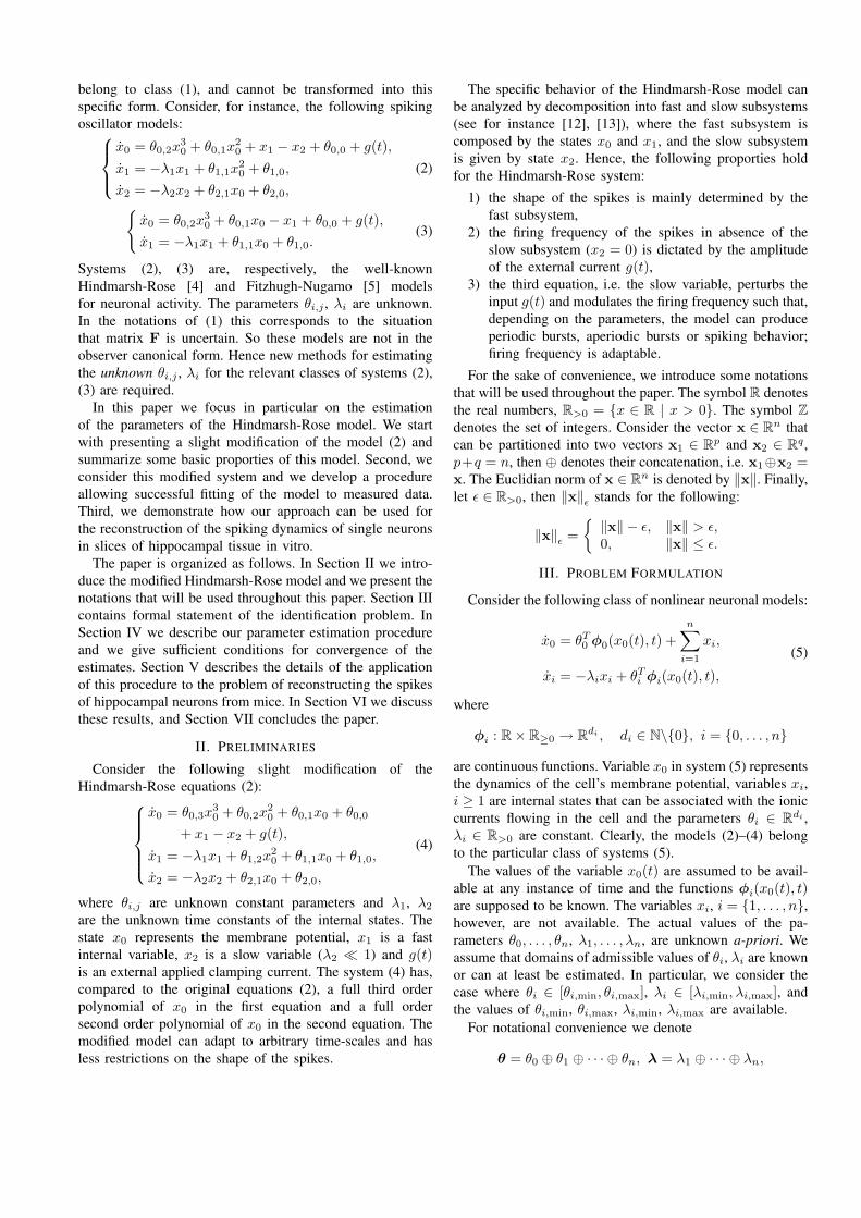
belong to class (1), and cannot be transformed into thisspecific form. Consider, for instance, the following spikingoscillator models:
x0 = θ0,2x30 + θ0,1x
20 + x1 − x2 + θ0,0 + g(t),
x1 = −λ1x1 + θ1,1x20 + θ1,0,
x2 = −λ2x2 + θ2,1x0 + θ2,0,
(2)
x0 = θ0,2x
30 + θ0,1x0 − x1 + θ0,0 + g(t),
x1 = −λ1x1 + θ1,1x0 + θ1,0.(3)
Systems (2), (3) are, respectively, the well-knownHindmarsh-Rose [4] and Fitzhugh-Nugamo [5] modelsfor neuronal activity. The parameters θi,j , λi are unknown.In the notations of (1) this corresponds to the situationthat matrix F is uncertain. So these models are not in theobserver canonical form. Hence new methods for estimatingthe unknown θi,j , λi for the relevant classes of systems (2),(3) are required.
In this paper we focus in particular on the estimationof the parameters of the Hindmarsh-Rose model. We startwith presenting a slight modification of the model (2) andsummarize some basic proporties of this model. Second, weconsider this modified system and we develop a procedureallowing successful fitting of the model to measured data.Third, we demonstrate how our approach can be used forthe reconstruction of the spiking dynamics of single neuronsin slices of hippocampal tissue in vitro.
The paper is organized as follows. In Section II we intro-duce the modified Hindmarsh-Rose model and we present thenotations that will be used throughout this paper. Section IIIcontains formal statement of the identification problem. InSection IV we describe our parameter estimation procedureand we give sufficient conditions for convergence of theestimates. Section V describes the details of the applicationof this procedure to the problem of reconstructing the spikesof hippocampal neurons from mice. In Section VI we discussthese results, and Section VII concludes the paper.
II. PRELIMINARIES
Consider the following slight modification of theHindmarsh-Rose equations (2):
x0 = θ0,3x30 + θ0,2x
20 + θ0,1x0 + θ0,0
+ x1 − x2 + g(t),
x1 = −λ1x1 + θ1,2x20 + θ1,1x0 + θ1,0,
x2 = −λ2x2 + θ2,1x0 + θ2,0,
(4)
where θi,j are unknown constant parameters and λ1, λ2
are the unknown time constants of the internal states. Thestate x0 represents the membrane potential, x1 is a fastinternal variable, x2 is a slow variable (λ2 1) and g(t)is an external applied clamping current. The system (4) has,compared to the original equations (2), a full third orderpolynomial of x0 in the first equation and a full ordersecond order polynomial of x0 in the second equation. Themodified model can adapt to arbitrary time-scales and hasless restrictions on the shape of the spikes.
The specific behavior of the Hindmarsh-Rose model canbe analyzed by decomposition into fast and slow subsystems(see for instance [12], [13]), where the fast subsystem iscomposed by the states x0 and x1, and the slow subsystemis given by state x2. Hence, the following proporties holdfor the Hindmarsh-Rose system:
1) the shape of the spikes is mainly determined by thefast subsystem,
2) the firing frequency of the spikes in absence of theslow subsystem (x2 = 0) is dictated by the amplitudeof the external current g(t),
3) the third equation, i.e. the slow variable, perturbs theinput g(t) and modulates the firing frequency such that,depending on the parameters, the model can produceperiodic bursts, aperiodic bursts or spiking behavior;firing frequency is adaptable.
For the sake of convenience, we introduce some notationsthat will be used throughout the paper. The symbol R denotesthe real numbers, R>0 = x ∈ R | x > 0. The symbol Zdenotes the set of integers. Consider the vector x ∈ Rn thatcan be partitioned into two vectors x1 ∈ Rp and x2 ∈ Rq,p+q = n, then ⊕ denotes their concatenation, i.e. x1⊕x2 =x. The Euclidian norm of x ∈ Rn is denoted by ‖x‖. Finally,let ε ∈ R>0, then ‖x‖ε stands for the following:
‖x‖ε =‖x‖ − ε, ‖x‖ > ε,0, ‖x‖ ≤ ε.
III. PROBLEM FORMULATION
Consider the following class of nonlinear neuronal models:
x0 = θT0 φ0(x0(t), t) +
n∑i=1
xi,
xi = −λixi + θTi φi(x0(t), t),
(5)
where
φi : R× R≥0 → Rdi , di ∈ N\0, i = 0, . . . , n
are continuous functions. Variable x0 in system (5) representsthe dynamics of the cell’s membrane potential, variables xi,i ≥ 1 are internal states that can be associated with the ioniccurrents flowing in the cell and the parameters θi ∈ Rdi ,λi ∈ R>0 are constant. Clearly, the models (2)–(4) belongto the particular class of systems (5).
The values of the variable x0(t) are assumed to be avail-able at any instance of time and the functions φi(x0(t), t)are supposed to be known. The variables xi, i = 1, . . . , n,however, are not available. The actual values of the pa-rameters θ0, . . . , θn, λ1, . . . , λn, are unknown a-priori. Weassume that domains of admissible values of θi, λi are knownor can at least be estimated. In particular, we consider thecase where θi ∈ [θi,min, θi,max], λi ∈ [λi,min, λi,max], andthe values of θi,min, θi,max, λi,min, λi,max are available.
For notational convenience we denote
θ = θ0 ⊕ θ1 ⊕ · · · ⊕ θn, λ = λ1 ⊕ · · · ⊕ λn,
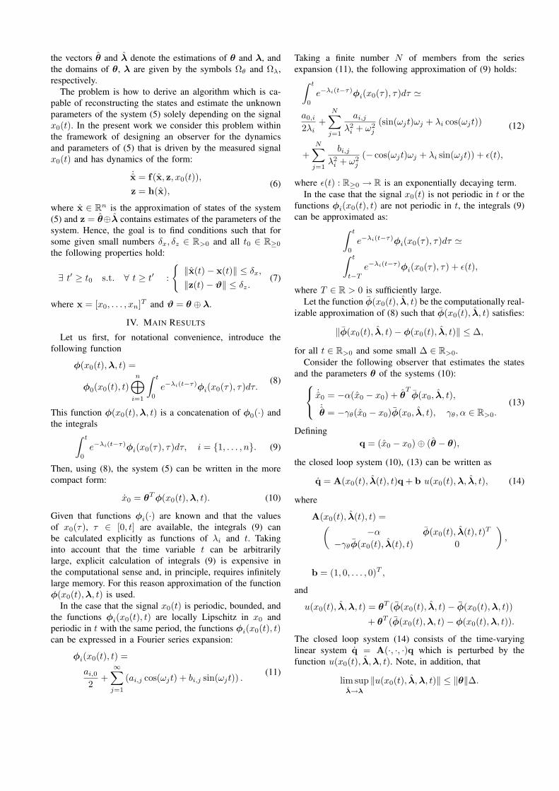
the vectors θ and λ denote the estimations of θ and λ, andthe domains of θ, λ are given by the symbols Ωθ and Ωλ,respectively.
The problem is how to derive an algorithm which is ca-pable of reconstructing the states and estimate the unknownparameters of the system (5) solely depending on the signalx0(t). In the present work we consider this problem withinthe framework of designing an observer for the dynamicsand parameters of (5) that is driven by the measured signalx0(t) and has dynamics of the form:
˙x = f(x, z, x0(t)),z = h(x),
(6)
where x ∈ Rn is the approximation of states of the system(5) and z = θ⊕λ contains estimates of the parameters of thesystem. Hence, the goal is to find conditions such that forsome given small numbers δx, δz ∈ R>0 and all t0 ∈ R≥0
the following properties hold:
∃ t′ ≥ t0 s.t. ∀ t ≥ t′ :
‖x(t)− x(t)‖ ≤ δx,
‖z(t)− ϑ‖ ≤ δz.(7)
where x = [x0, . . . , xn]T and ϑ = θ ⊕ λ.
IV. MAIN RESULTS
Let us first, for notational convenience, introduce thefollowing function
φ(x0(t),λ, t) =
φ0(x0(t), t)n⊕
i=1
∫ t
0
e−λi(t−τ)φi(x0(τ), τ)dτ.(8)
This function φ(x0(t),λ, t) is a concatenation of φ0(·) andthe integrals∫ t
0
e−λi(t−τ)φi(x0(τ), τ)dτ, i = 1, . . . , n. (9)
Then, using (8), the system (5) can be written in the morecompact form:
x0 = θT φ(x0(t),λ, t). (10)
Given that functions φi(·) are known and that the valuesof x0(τ), τ ∈ [0, t] are available, the integrals (9) canbe calculated explicitly as functions of λi and t. Takinginto account that the time variable t can be arbitrarilylarge, explicit calculation of integrals (9) is expensive inthe computational sense and, in principle, requires infinitelylarge memory. For this reason approximation of the functionφ(x0(t),λ, t) is used.
In the case that the signal x0(t) is periodic, bounded, andthe functions φi(x0(t), t) are locally Lipschitz in x0 andperiodic in t with the same period, the functions φi(x0(t), t)can be expressed in a Fourier series expansion:
φi(x0(t), t) =
ai,0
2+
∞∑j=1
(ai,j cos(ωjt) + bi,j sin(ωjt)) .(11)
Taking a finite number N of members from the seriesexpansion (11), the following approximation of (9) holds:∫ t
0
e−λi(t−τ)φi(x0(τ), τ)dτ '
a0,i
2λi+
N∑j=1
ai,j
λ2i + ω2
j
(sin(ωjt)ωj + λi cos(ωjt))
+N∑
j=1
bi,j
λ2i + ω2
j
(− cos(ωjt)ωj + λi sin(ωjt)) + ε(t),
(12)
where ε(t) : R≥0 → R is an exponentially decaying term.In the case that the signal x0(t) is not periodic in t or the
functions φi(x0(t), t) are not periodic in t, the integrals (9)can be approximated as:∫ t
0
e−λi(t−τ)φi(x0(τ), τ)dτ '∫ t
t−T
e−λi(t−τ)φi(x0(τ), τ) + ε(t),
where T ∈ R > 0 is sufficiently large.Let the function φ(x0(t), λ, t) be the computationally real-
izable approximation of (8) such that φ(x0(t), λ, t) satisfies:
‖φ(x0(t), λ, t)− φ(x0(t), λ, t)‖ ≤ ∆,
for all t ∈ R>0 and some small ∆ ∈ R>0.Consider the following observer that estimates the states
and the parameters θ of the systems (10): ˙x0 = −α(x0 − x0) + θTφ(x0, λ, t),
˙θ = −γθ(x0 − x0)φ(x0, λ, t), γθ, α ∈ R>0.
(13)
Definingq = (x0 − x0)⊕ (θ − θ),
the closed loop system (10), (13) can be written as
q = A(x0(t), λ(t), t)q + b u(x0(t),λ, λ, t), (14)
where
A(x0(t), λ(t), t) =(−α φ(x0(t), λ(t), t)T
−γθφ(x0(t), λ(t), t) 0
),
b = (1, 0, . . . , 0)T ,
and
u(x0(t), λ,λ, t) = θT (φ(x0(t), λ, t)− φ(x0(t),λ, t))
+ θT (φ(x0(t),λ, t)− φ(x0(t),λ, t)).
The closed loop system (14) consists of the time-varyinglinear system q = A(·, ·, ·)q which is perturbed by thefunction u(x0(t), λ,λ, t). Note, in addition, that
lim supλ→λ
‖u(x0(t), λ,λ, t)‖ ≤ ‖θ‖∆.
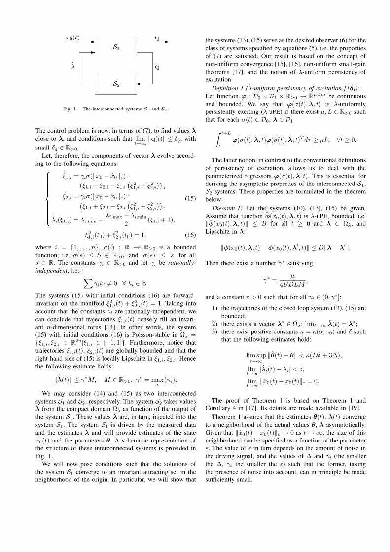
x0(t) q
qλ
S1
S2
Fig. 1. The interconnected systems S1 and S2.
The control problem is now, in terms of (7), to find values λclose to λ, and conditions such that lim
t→∞‖q(t)‖ ≤ δq, with
small δq ∈ R>0.Let, therefore, the components of vector λ evolve accord-
ing to the following equations:
ξ1,i = γiσ(‖x0 − x0‖ε) ·(ξ1,i − ξ2,i − ξ1,i
(ξ21,i + ξ2
2,i
)),
ξ2,i = γiσ(‖x0 − x0‖ε) ·(ξ1,i + ξ2,i − ξ2,i
(ξ21,i + ξ2
2,i
)),
λi(ξ1,i) = λi,min +λi,max − λi,min
2(ξ1,i + 1),
(15)
ξ21,i(t0) + ξ2
2,i(t0) = 1, (16)
where i = 1, . . . , n, σ(·) : R → R≥0 is a boundedfunction, i.e. σ(s) ≤ S ∈ R>0, and |σ(s)| ≤ |s| for alls ∈ R. The constants γi ∈ R>0 and let γi be rationally-independent, i.e.: ∑
γiki 6= 0, ∀ ki ∈ Z.
The systems (15) with initial conditions (16) are forward-invariant on the manifold ξ2
1,i(t) + ξ22,i(t) = 1. Taking into
account that the constants γi are rationally-independent, wecan conclude that trajectories ξ1,i(t) densely fill an invari-ant n-dimensional torus [14]. In other words, the system(15) with initial conditions (16) is Poisson-stable in Ωx =ξ1,i, ξ2,i ∈ R2n|ξ1,i ∈ [−1, 1]. Furthermore, notice thattrajectories ξ1,i(t), ξ2,i(t) are globally bounded and that theright-hand side of (15) is locally Lipschitz in ξ1,i, ξ2,i. Hencethe following estimate holds:
‖ ˙λ(t)‖ ≤ γ∗M, M ∈ R>0, γ∗ = max
iγi.
We may consider (14) and (15) as two interconnectedsystems S1 and S2, respectively. The system S2 takes valuesλ from the compact domain Ωλ as function of the output ofthe system S1. These values λ are, in turn, injected into thesystem S1. The system S1 is driven by the measured dataand the estimates λ and will provide estimates of the statex0(t) and the parameters θ. A schematic representation ofthe structure of these interconnected systems is provided inFig. 1.
We will now pose conditions such that the solutions ofthe system S1 converge to an invariant attracting set in theneighborhood of the origin. In particular, we will show that
the systems (13), (15) serve as the desired observer (6) for theclass of systems specified by equations (5), i.e. the proportiesof (7) are satisfied. Our result is based on the concept ofnon-uniform convergence [15], [16], non-uniform small-gaintheorems [17], and the notion of λ-uniform persistency ofexcitation:
Definition 1 (λ-uniform persistency of excitation [18]):Let function ϕ : D0 × D1 × R≥0 → Rn×m be continuousand bounded. We say that ϕ(σ(t),λ, t) is λ-uniformlypersistently exciting (λ-uPE) if there exist µ,L ∈ R>0 suchthat for each σ(t) ∈ D0, λ ∈ D1∫ t+L
t
ϕ(σ(t),λ, t)ϕ(σ(t),λ, t)T dτ ≥ µI, ∀t ≥ 0.
The latter notion, in contrast to the conventional definitionsof persistency of excitation, allows us to deal with theparameterized regressors ϕ(σ(t),λ, t). This is essential forderiving the asymptotic properties of the interconnected S1,S2 systems. These properties are formulated in the theorembelow:
Theorem 1: Let the systems (10), (13), (15) be given.Assume that function φ(x0(t),λ, t) is λ-uPE, bounded, i.e.‖φ(x0(t),λ, t)‖ ≤ B for all t ≥ 0 and λ ∈ Ωλ, andLipschitz in λ:
‖φ(x0(t),λ, t)− φ(x0(t),λ′, t)‖ ≤ D‖λ− λ′‖.
Then there exist a number γ∗ satisfying
γ∗ =µ
4BDLM,
and a constant ε > 0 such that for all γi ∈ (0, γ∗]:
1) the trajectories of the closed loop system (13), (15) arebounded;
2) there exists a vector λ∗ ∈ Ωλ: limt→∞ λ(t) = λ∗;3) there exist positive constants κ = κ(α, γ0) and δ such
that the following estimates hold:
lim supt→∞
‖θ(t)− θ‖ < κ(Dδ + 3∆),
limt→∞
|λi(t)− λi| < δ,
limt→∞
‖x0(t)− x0(t)‖ε = 0.
The proof of Theorem 1 is based on Theorem 1 andCorollary 4 in [17]. Its details are made available in [19].
Theorem 1 assures that the estimates θ(t), λ(t) convergeto a neighborhood of the actual values θ, λ asymptotically.Given that ‖x0(t)− x0(t)‖ε → 0 as t →∞, the size of thisneighborhood can be specified as a function of the parameterε. The value of ε in turn depends on the amount of noise inthe driving signal, and the values of ∆ and γi (the smallerthe ∆, γi the smaller the ε) such that the former, takingthe presence of noise into account, can in principle be madesufficiently small.
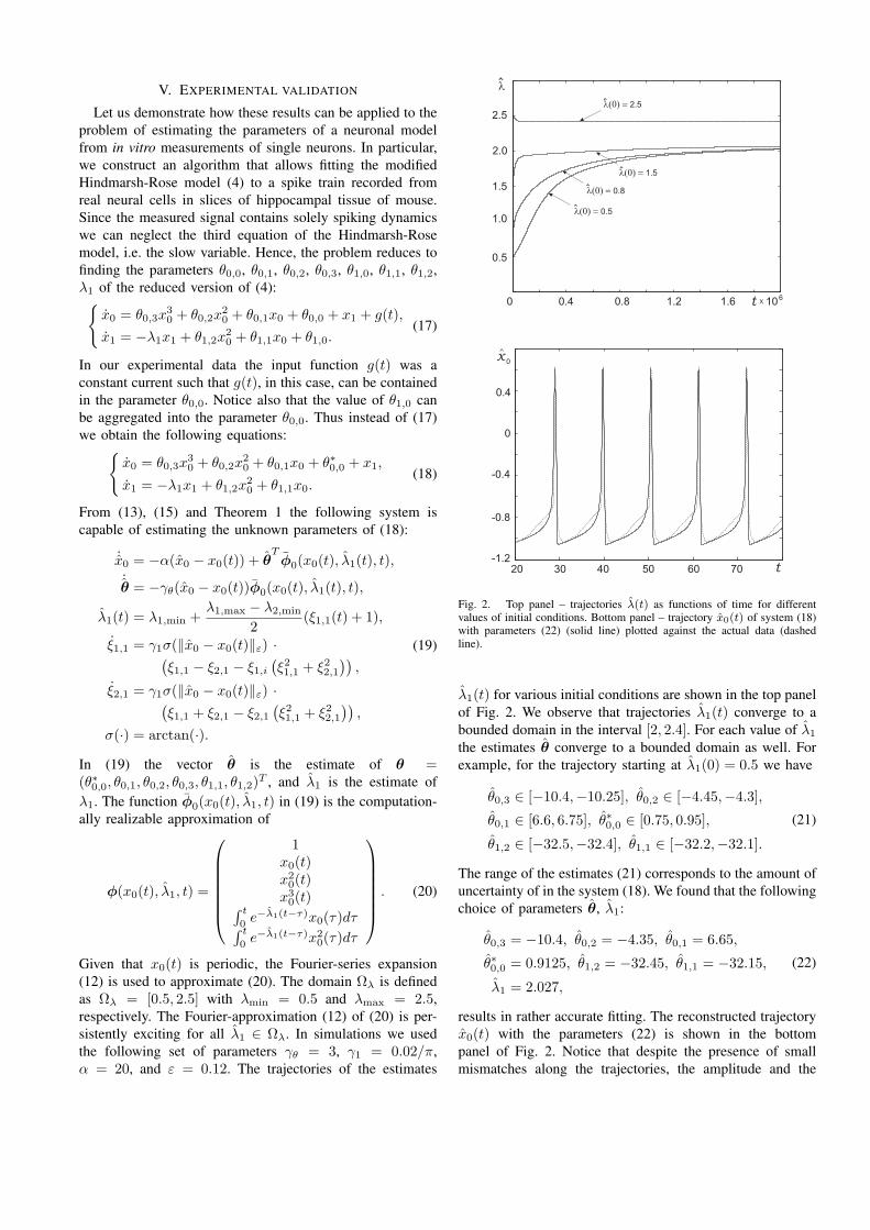
V. EXPERIMENTAL VALIDATION
Let us demonstrate how these results can be applied to theproblem of estimating the parameters of a neuronal modelfrom in vitro measurements of single neurons. In particular,we construct an algorithm that allows fitting the modifiedHindmarsh-Rose model (4) to a spike train recorded fromreal neural cells in slices of hippocampal tissue of mouse.Since the measured signal contains solely spiking dynamicswe can neglect the third equation of the Hindmarsh-Rosemodel, i.e. the slow variable. Hence, the problem reduces tofinding the parameters θ0,0, θ0,1, θ0,2, θ0,3, θ1,0, θ1,1, θ1,2,λ1 of the reduced version of (4):
x0 = θ0,3x30 + θ0,2x
20 + θ0,1x0 + θ0,0 + x1 + g(t),
x1 = −λ1x1 + θ1,2x20 + θ1,1x0 + θ1,0.
(17)
In our experimental data the input function g(t) was aconstant current such that g(t), in this case, can be containedin the parameter θ0,0. Notice also that the value of θ1,0 canbe aggregated into the parameter θ0,0. Thus instead of (17)we obtain the following equations:
x0 = θ0,3x30 + θ0,2x
20 + θ0,1x0 + θ∗0,0 + x1,
x1 = −λ1x1 + θ1,2x20 + θ1,1x0.
(18)
From (13), (15) and Theorem 1 the following system iscapable of estimating the unknown parameters of (18):
˙x0 = −α(x0 − x0(t)) + θTφ0(x0(t), λ1(t), t),
˙θ = −γθ(x0 − x0(t))φ0(x0(t), λ1(t), t),
λ1(t) = λ1,min +λ1,max − λ2,min
2(ξ1,1(t) + 1),
ξ1,1 = γ1σ(‖x0 − x0(t)‖ε) ·(ξ1,1 − ξ2,1 − ξ1,i
(ξ21,1 + ξ2
2,1
)),
ξ2,1 = γ1σ(‖x0 − x0(t)‖ε) ·(ξ1,1 + ξ2,1 − ξ2,1
(ξ21,1 + ξ2
2,1
)),
σ(·) = arctan(·).
(19)
In (19) the vector θ is the estimate of θ =(θ∗0,0, θ0,1, θ0,2, θ0,3, θ1,1, θ1,2)T , and λ1 is the estimate ofλ1. The function φ0(x0(t), λ1, t) in (19) is the computation-ally realizable approximation of
φ(x0(t), λ1, t) =
1x0(t)x2
0(t)x3
0(t)∫ t
0e−λ1(t−τ)x0(τ)dτ∫ t
0e−λ1(t−τ)x2
0(τ)dτ
. (20)
Given that x0(t) is periodic, the Fourier-series expansion(12) is used to approximate (20). The domain Ωλ is definedas Ωλ = [0.5, 2.5] with λmin = 0.5 and λmax = 2.5,respectively. The Fourier-approximation (12) of (20) is per-sistently exciting for all λ1 ∈ Ωλ. In simulations we usedthe following set of parameters γθ = 3, γ1 = 0.02/π,α = 20, and ε = 0.12. The trajectories of the estimates
2.5
2.0
1.5
1.0
0.5
0.40 0.8 1.2 1.6
l(0) = 2.5
l(0) = 1.5
l(0) = 0.5
l(0) = 0.8
t
l
<
<
<
<
<
106X
Fig. 2. Top panel – trajectories λ(t) as functions of time for differentvalues of initial conditions. Bottom panel – trajectory x0(t) of system (18)with parameters (22) (solid line) plotted against the actual data (dashedline).
λ1(t) for various initial conditions are shown in the top panelof Fig. 2. We observe that trajectories λ1(t) converge to abounded domain in the interval [2, 2.4]. For each value of λ1
the estimates θ converge to a bounded domain as well. Forexample, for the trajectory starting at λ1(0) = 0.5 we have
θ0,3 ∈ [−10.4,−10.25], θ0,2 ∈ [−4.45,−4.3],
θ0,1 ∈ [6.6, 6.75], θ∗0,0 ∈ [0.75, 0.95],
θ1,2 ∈ [−32.5,−32.4], θ1,1 ∈ [−32.2,−32.1].
(21)
The range of the estimates (21) corresponds to the amount ofuncertainty of in the system (18). We found that the followingchoice of parameters θ, λ1:
θ0,3 = −10.4, θ0,2 = −4.35, θ0,1 = 6.65,
θ∗0,0 = 0.9125, θ1,2 = −32.45, θ1,1 = −32.15,
λ1 = 2.027,
(22)
results in rather accurate fitting. The reconstructed trajectoryx0(t) with the parameters (22) is shown in the bottompanel of Fig. 2. Notice that despite the presence of smallmismatches along the trajectories, the amplitude and the
shape of the spikes do closely follow the measured responseof the hippocampal neuron.
VI. DISCUSSION
We showed that the spiking dynamics measured from asingle neuron from the hippocampal area of mouse can bereconstructed with the modified Hindmarsh-Rose model (4).Moreover, the estimated parameters of the model convergeto small bounded domains. The size of these domains can,in principle, be decreased by assigning a smaller valueto the parameter ε. However, it might be possible thatthe model is not accurate enough to describe the spikeswith such precision. The fact that the modified model’sparameters θ0,1, θ1,1 6= 0 indicates that the equations of theoriginal Hindmarsh-Rose model are too restricted for properparameter fitting and our choice to use the modified modelis justified.
We considered a simplified case where the clampingcurrent applied to the neuron was constant and the neuronproduced simple spiking behavior. In general, the outputfunction of neurons is more complicated. Bursting sequences,for instance, are noticed in neurons of the pond snail Lym-naea [4] and firing frequency adaptation often occurs whenthe neuron is stimulated with block shaped currents. In orderto mimic this more complicated behavior, the full set ofequations of the modified Hindmarsh-Rose model should betaken into account.
VII. CONCLUSION
We presented a method to estimate the parameters of sys-tems that can not be transformed into the observer canonicalform. The proposed method can be applied to systems thatare of the class (5), such as (mathematical) models thatmimic neuronal behavior. We demonstrated a direct applica-tion of the method by means of a successful reconstructionof the states and estimations of the parameters of a modifiedHindmarsh-Rose model driven by spikes recorded from asingle neuron in vitro.
ACKNOWLEDGEMENTS
The authors gratefully thank Dr. Alexey Semyanov and Dr.Inseon Song of the Semyanov Research Unit, Riken BSI, forperforming the single neuron recordings.
REFERENCES
[1] C. Koch, Biophysics of Computation. Information Processing in SignleNeurons. Oxford University Press, 2002.
[2] A. Hodgkin and A. Huxley, “A quantitative description of membranecurrent and its application to conduction and excitation in nerve,” J.Physiol., vol. 117, pp. 500–544, 1952.
[3] E. M. Izhikevich, “Neural excitability, spiking, and bursting,” Inter-national Journal of Bifurcation and Chaos, vol. 10, pp. 1171–1266,2000.
[4] J. Hindmarsh and R. Rose, “A model of neuronal bursting using threecoupled first order differential equations,” Proc. R. Soc. Lond., vol. B221, no. 1222, pp. 87–102, 1984.
[5] R. FitzHugh, “Impulses and physiological states in theoretical modelsof nerve membrane,” Biophysical Journal, vol. 1, pp. 445–466, 1961.
[6] E. M. Izhikevich, “Which model to use for cortical spiking neurons?”IEEE Transactions on Neural Networks, vol. 15, pp. 1063–1070, 2004.
[7] L. Ljung, System Identification: Theory for the User. Prentice-Hall,1999.
[8] S. Sastry, Nonlinear Systems: Analysis, Stability and Control.Springer, 1999.
[9] G. Bastin and M. Gevers, “Stable adaptive observers for nonlineartime-varying systems,” IEEE Trans. on Automatic Control, vol. 33,no. 7, pp. 650–658, 1988.
[10] R. Marino and P. Tomei, “Global adaptive output-feedback controlof nonlinear systems, part I: Linear parameterization,” IEEE Trans.Automatic Control, vol. 38, no. 1, pp. 17–32, 1993.
[11] ——, “Adaptive observers with arbitrary exponential rate of conver-gence for nonlinear systems,” IEEE Trans. Automatic Control, vol. 40,no. 7, pp. 1300–1304, 1995.
[12] V. Belykh, I. Belykh, M. Colding-Jørgensen, and E. Mosekilde, “Ho-moclinic bifurcations leading to the emergence of bursting oscillationsin cell models,” Euro. Phys. J. E, vol. 3, pp. 205–219, 2000.
[13] D. Terman, “Chaotic Spikes Arising from a Model of Bursting inExcitable Membranes,” SIAM J. Appl. Math., vol. 51, pp. 1418–1450,1991.
[14] V. Arnold, Mathematical Methods in Classical Mechanics. Springer-Verlag, 1978.
[15] J. Milnor, “On the concept of attractor,” Commun. Math. Phys., vol. 99,pp. 177–195, 1985.
[16] A. Gorban, “Singularities of transition processes in dynamical systems:Qualitative theory of critical delays,” Electronic Journal of DifferentialEquations, vol. Monograph 05, 2004.
[17] I. Tyukin, E. Steur, H. Nijmeijer, and C. van Leeuwen, “Non-uniformsmall-gain theorems for systems with unstable invariant sets,” SIAMJournal on Control and Optimization, (accepted, preprint available athttp://arxiv.org/abs/math.DS/0612381).
[18] A. Loria and E. Panteley, “Uniform exponential stability of linear time-varying systems: revisited,” Systems and Control Letters, vol. 47, no. 1,pp. 13–24, 2003.
[19] I. Tyukin, E. Steur, H. Nijmeijer, and C. van Leeuwen, “Identificationand Modelling of Neural Dynamics,” Manuscript in preparation,preprints are available upon request.
Non-uniform Small-gain Theorems forSystems with Unstable Invariant Sets
Ivan Tyukin∗, Erik Steur†, Henk Nijmeijer ‡, Cees van Leeuwen§
October 17, 2006
Abstract
We consider the problem of asymptotic convergence to invariant sets in intercon-nected nonlinear dynamic systems. Standard approaches often require that the invari-ant sets be uniformly attracting. e.g. stable in the Lyapunov sense. This, however, isneither a necessary requirement, nor is it always useful. Systems may, for instance, beinherently unstable (e.g. intermittent, itinerant, meta-stable) or the problem statementmay include requirements that cannot be satisfied with stable solutions. This is oftenthe case in general optimization problems and in nonlinear parameter identificationor adaptation. Conventional techniques for these cases rely either on detailed knowl-edge of the system’s vector-fields or require boundeness of its states. The presentlyproposed method relies only on estimates of the input-output maps and steady-statecharacteristics. The method requires the possibility of representing the system as an in-terconnection of a stable, contracting, and an unstable, exploratory part. We illustratewith examples how the method can be applied to problems of analyzing the asymptoticbehavior of locally unstable systems as well as to problems of parameter identificationand adaptation in the presence of nonlinear parametrizations. The relation of ourresults to conventional small-gain theorems is discussed.
Keywords: non-uniform convergence, weakly attracting sets, small-gain theorems, input-output stability
1 Notation
Throughout the paper we use the following notational conventions. Symbol R denotes thefield of real numbers, symbol R+ stands for the following subset of R: R+ = x ∈ R| x ≥
∗Corresponding author. Laboratory for Perceptual Dynamics, RIKEN (Institute for Physical andChemical Research) Brain Science Institute, 2-1, Hirosawa, Wako-shi, Saitama, 351-0198, Japan, e-mail:[email protected]
†Dept. of Mechanical Engineering, Dynamics and Control, Eindhoven University of Technology, P.O. Box513 5600 MB, Eindhoven, The Netherlands, e-mail: [email protected]
‡Dept. of Mechanical Engineering, Dynamics and Control, Eindhoven University of Technology, P.O. Box513 5600 MB, Eindhoven, The Netherlands, e-mail: [email protected]
§Laboratory for Perceptual Dynamics, RIKEN (Institute for Physical and Chemical Research) BrainScience Institute, 2-1, Hirosawa, Wako-shi, Saitama, 351-0198, Japan, e-mail: [email protected]
1
0; N and Z denote the set of natural numbers and its extension to the negative domainrespectively.
Let Ω be a set, by symbol SΩ we denote the set of all subsets of Ω. Symbol Ck denotesthe space of functions that are at least k times differentiable; K denotes the class of all strictlyincreasing functions κ : R+ → R+ such that κ(0) = 0. If, in addition, lims→∞ κ(s) = ∞we say that κ ∈ K∞. Further, Ke (or Ke,∞) denotes the class of functions of which therestriction to the interval [0,∞) belongs to K (or K∞). Symbol KL denotes the class offunctions β : R+ × R+ → R+ such that β(·, 0) ∈ K and β(0, ·) is monotonically decreasing.
Let x ∈ Rn and x can be partitioned into two vectors x1 ∈ Rq, x1 = (x11, . . . , x1q)T ,
x2 ∈ Rp, x2 = (x21, . . . , x2p)T with q+p = n, then⊕ denotes their concatenation: x = x1⊕x2.
The symbol ‖x‖ denotes the Euclidian norm in x ∈ Rn. By Ln∞[t0, T ] we denote the
space of all functions f : R+ → Rn such that ‖f‖∞,[t0,T ] = sup‖f(t)‖, t ∈ [t0, T ] < ∞, and‖f‖∞,[t0,T ] stands for the Ln
∞[t0, T ] norm of f(t). Let A be a set in Rn and ‖ · ‖ be the usualEuclidean norm in Rn. By the symbol ‖·‖A we denote the following induced norm:
‖x‖A = infq∈A
‖x− q‖
Let ∆ ∈ R+ then the notation ‖x‖A∆stands for the following equality:
‖x‖A∆=
‖x‖A −∆, ‖x‖A > ∆0, ‖x‖A ≤ ∆
The symbol ‖·‖A∞,[t0,t] is defined as follows:
‖x(τ)‖A∞,[t0,t] = supτ∈[t0,t]
‖x(τ)‖A
2 Introduction
In many fields of science, from systems and control theory to physics, chemistry, and biology,it is of fundamental importance to analyze the asymptotic behavior of dynamical systems.Most of these analyses are based around the concept of Lyapunov stability [15], [32], [31], i.e.continuity of the flow x(t,x0) : R+×Rn → Ln
∞[t0,∞] with respect to x0 [18], in combinationwith the standard notion of an attracting set [9]:
Definition 1 A set A is an attracting set iff it isi) closed, invariant, andii) for some neighborhood V of A and for all x0 ∈ V the following conditions hold:
x(t,x0) ∈ V ∀ t ≥ 0; (1)
limt→∞
‖x(t,x0)‖A = 0 (2)
Condition (1) in Definition 1 stipulates the existence of a trapping region V which is aneighborhood ofA. Condition (2) ensures attractivity, or convergence to S. Due to condition(1), convergence to A is uniform with respect to x0 in the neighborhood of A, i.e. everytrajectory which starts in V remains in V for t ≥ 0 and converges to A at t →∞.
Although the conventional concepts of attracting set and Lyapunov stability are a power-ful tandem in various applications, some problems cannot be solved within this framework.
2
Condition (1), for example, could be violated in systems with intermittent, itinerant, ormeta-stable dynamics. In general the condition does not hold when the system dynamics,loosely speaking, is exploring rather than contracting. Such systems appear naturally in thecontext of global optimization. For instance, in [22] finding the global minimum of a differ-entiable cost function Q : Rn → R+ in a bounded subset Ωx ⊂ Rn is achieved by splittingthe search procedure into a locally attracting gradient Sa, and a wandering part Sw:
Sa : x = −µx∂Q(x)
∂x+ µtT (t), µx, µt ∈ R+
Sw : T (t) = ht,x(t), h : R+ × Ln∞[t0, t] → Ln
∞[t0, t](3)
The trace function, T (t), in (3) is supposed to cover (i.e. be dense in) the whole searchingdomain Ωx. Even though the results in [22] are purely simulation studies, they illustratethe superior performance of algorithms (3) in a variety of benchmark problems comparedto standard local minimizers and classical methods of global optimization. AbandoningLyapunov stability is likewise advantageous in problems of identification and adaptation inthe presence of general nonlinear parameterization [28], in manoeuvring and path searching[25], and in decision making in intelligent systems [29], [30]. Systems with attracting, yetunstable invariant sets are relevant for modelling complex behavior in biological and physicalsystems [2]. Last but not least, Lyapunov-unstable attracting sets are relevant in problemsof synchronization [5], [19], [26]1.
Even when it is appropriate to consider a system as stable, we may be limited in oursuccess in meeting the requirement to identify a proper Lyuapunov function.This is thecase, for instance, when the system’s dynamics is only partially known. Trading stabilityrequirements for the sake of convergence might be a possible remedy. Known results in thisdirection can be found in [11], [21]2.
In all the cases that are problematic under condition (1) of Definition 1, condition (2) –convergence of x(t,x0) to an invariant set A, is still a requirement that has to be met. Inorder to treat these cases analytically we shall, first of all, move from the standard conceptof attracting sets in Definition 1 to one that does not assume that the basin of attraction isnecessarily a neighborhood of the invariant set A. In other words we shall allow convergencewhich is not uniform in initial conditions. This requirement is captured by the concept ofweak, or Milnor attraction [17]:
Definition 2 A set A is weakly attracting, or Milnor attracting set iffi) it is closed, invariant andii) for some set V (not necessarily a neighborhood of A) with strictly positive measure
and for all x0 ∈ V limiting relation (2) holds
Conventional methods such as La Salle’s invariance principle [14] or center manifoldtheory [7] can, in principle, address the issue of convergence to weak equilibria. They do so,however, at the expense of requiring detailed knowledge of the vector-fields of the ordinarydifferential equations of the model. When such information is not available the system can
1See also [20] where the striking difference between stable and ”almost stable” synchronization in termsof the coupling strengthes for a pair of the Lorenz oscillators is demonstrated analytically.
2In the Examples section, we demonstrate how explorative dynamics can solve the problem of simultaneousstate and parameter observation for a system which cannot be transformed into a canonical adaptive observerform [3].
3

be thought of as a mere interconnection of input-output maps. Small-gain theorems [33],[12]are usually efficient in this case. These results, however, apply only under the assumptionof stability of each component in the interconnection.
In the present study we aim to find a proper balance between the generality of input-output approaches [33], [12] in the analysis of convergence and the specificity of the funda-mental notions of limit sets and invariance that play a central role in [14], [7]. The objectof our study is a class of systems that can be decomposed into an attracting, or stable,component Sa and an exploratory, generally unstable, part Sw. Typical systems of this classare nonlinear systems in cascaded form
Sa : x = f(x, z),
Sw : z = q(z,x)(4)
where the zero solution of the x-subsystem is asymptotically stable in the absence of input z,and the state of the z-subsystem are functions of
∫ t
t0‖x(τ)‖dτ . Even when both subsystems
in (4) are stable and the x-subsystem does not depend on state z, the cascade can stillbe unstable [1]. We show, however, that for unstable interconnections (4), under certainconditions that involve only input-to-state properties of Sa and Sw, there is a set V inthe system state space, such that trajectories starting in V remain bounded. The result isformally stated in Theorem 1. In case an additional measure of invariance is defined forSa (in our case a steady-state characteristic), a weak, Milnor attracting set emerges. Itslocation is completely determined by the zeros of the steady-state response of system Sa.
We demonstrate how this basic result can be used in problems of design and analysisof control systems and identification/adaptation algorithms. In particular, we present anadaptive observer of state and parameter values for uncertain systems which cannot betransformed into a canonic adaptive observer form [3]. In the Examples section we presentan application of this result to the problem of reconstructing a dynamic model of neuronalcell activity.
The paper is organized as follows. In Section 3 we formally state the problem and providespecific assumptions for the class of systems under consideration. Section 4 contains the mainresults of our present study. In Section 5 we provide several corollaries of the main resultthat apply to specific problems. Section 6 contains examples, and Section 7 concludes thepaper.
3 Problem Formulation
Consider a system that can be decomposed into two interconnected subsystems, Sa and Sw:
Sa : (ua,x0) 7→ x(t)
Sw : (uw, z0) 7→ z(t)(5)
where ua ∈ Ua ⊆ L∞[t0,∞], uw ∈ Uw ⊆ L∞[t0,∞] are the spaces of inputs to Sa and Sw,respectively x0 ∈ Rn, z0 ∈ Rm represent initial conditions, and x(t) ∈ X ⊆ Ln
∞[t0,∞],z(t) ∈ Z ⊆ Lm
∞[t0,∞] are the system states.System Sa represents the contracting dynamics. More precisely, we require that Sa is
input-to-state stable3 [23] with respect to a compact set A:
3In general, as will be demonstrated with examples, our analysis can be carried out for (integral) input-to-output/state stable systems as well.
4
Assumption 1 (Contracting dynamics)
Sa : ‖x(t)‖A ≤ β(‖x(t0)‖A , t− t0) + c‖ua(t)‖∞,[t0,t], ∀t0 ∈ R+, t ≥ t0 (6)
where the function β(·, ·) ∈ KL, and c > 0 is some positive constant.
The function β(·, ·) in (6) specifies the contraction property of the unperturbed dynamics ofSa. In other words it models the rate with which the system forgets its initial conditions x0,if left unperturbed. Propagation of the input to output is estimated in terms of a continuousmapping, c‖ua(t)‖∞,[t0,t], which, in our case, is chosen for simplicity to be linear. Notice thatthis mapping should not necessarily be contracting. In what follows we will assume that thefunction β(·, ·) and constant c are known or can be estimated a-priori.
For systems Sa, of which a model is given by a system of ordinary differential equations
x = fx(x, ua), fx(·, ·) ∈ C1, (7)
Assumption 1 is equivalent, for instance, to the combination of the following properties4:
1. let ua(t) ≡ 0 for all t, then set A is Lyapunov stable and globally attracting for (7);
2. for all ua ∈ Ua and x0 ∈ Rn there exists a non-decreasing function κ : R+ → R+ :κ(0) = 0 such that
inft∈[0,∞)
‖x(t)‖A ≤ κ(‖ua(t)‖∞,[t0,∞))
The system Sw stands for the searching or wandering dynamics. We will consider Sw
subject to the following conditions:
Assumption 2 (Wandering dynamics) The system Sw is forward-complete:
uw(t) ∈ Uw ⇒ z(t) ∈ Z, ∀ t ≥ t0, t0 ∈ R+
and there exists an ”output” function h : Rm → R, and two ”bounding” functions γ0 ∈ K∞,e,γ ∈ K∞,e such that the following integral inequality holds:
Sw :
∫ t
t0
γ1(uw(τ))dτ ≤ h(z(t0))− h(z(t)) ≤∫ t
t0
γ0(uw(τ))dτ, ∀ t ≥ t0, t0 ∈ R+ (8)
In case system Sw is specified in terms of vector-fields
z = fz(z, uw), fz(·, ·) ∈ C1, (9)
Assumption 2 can be viewed, for example, as postulating the existence of a function h :Rm → R+ of which the evolution in time is a mere integration of the input uw(t). In general,for uw : uw(t) ≥ 0 ∀ t ∈ R+, inequality (8) implies monotonicity of function h(z(t)) in t.Regarding the function γ0(·) in (8), we assume that for any M ∈ R+ there exist functionsγ0,1 : R+ → R+ and γ0,2 : R+ → R+, such that
γ0(a · b) ≤ γ0,1(a) · γ0,2(b),∀ a, b ∈ [0,M ]. (10)
4For a comprehensive characterization of the input-to-state stability and detailed mathematical argumentswe refer to the paper by E.D. Sontag and Y. Wang [24].
5
ab
Figure 1: a. The class of interconnected systems Sa and Sw. System Sa, the “contracting system”,has an attracting invariant setA in its state space, system Sw does not necessarily have an attractingset. It represents the “wandering” dynamics. A typical example of such behavior is the dynamicsof the flow in a neighborhood of a saddle point in three-dimensional space (diagram b).
Requirement (10) is a technical assumption which will be used in the formulation and proofof the main results of the paper. Yet, it is not too restrictive; it holds, for instance, for awide class of locally Lipschitz functions γ0(·) : γ0(a · b) ≤ L0(M) · (a · b), L0(M) ∈ R+.Another example for which the assumption holds is the class of polynomial functions γ0(·) :γ0(a · b) = (a · b)p = ap · bp, p > 0. No further restrictions will be imposed a-priori on Sa, Sw.
Now consider the interconnection of (6), (8) with coupling ua(t) = h(z(t)), and us(t) =‖x(t)‖A. Equations for the combined system can be written as:
‖x(t)‖A ≤β(‖x(t0)‖A , t− t0) + c‖h(z(t))‖∞,[t0,t]∫ t
t0
γ1(‖x(τ)‖A)dτ ≤h(z(t0))− h(z(t)) ≤∫ t
t0
γ0(‖x(τ)‖A)dτ,(11)
A diagram illustrating the general structure of the entire system (11) is given in figure 1.Equations (11) capture the relevant interplay between contracting, Sa, and wandering,
Sw, dynamics inherent to a variety of searching strategies in the realm of optimization, (3),and interconnections (4) in general systems theory. In addition, this kind of interconnectiondescribes the behavior of systems which undergo transcritical or saddle-node bifurcations.Consider for instance the following system:
x1 = −x1 + x2
x2 = ε + γx21, γ > 0
(12)
where the parameter ε varies from negative to positive values. At ε = 0 stable and unstableequilibria collide leading to the cascade satisfying equations (11). An alternative bifurcationscenario could be represented by system:
x1 = −x1 + x2
x2 = ε + γx22, γ > 0,
(13)
In this case, however, the dynamics of the variable x2 is independent of x1, and analysis ofasymptotic behavior of (13) reduces to the analysis of each equation separately. Thus systems
6
like (13) are easier to deal with than (12). This constitutes an additional motivation for thepresent approach.
When analyzing the asymptotic behavior of interconnection (11) we will address thefollowing set of questions: is there a set (a weak trapping set in the system state space) suchthat the trajectories which start in this set are bounded? It is natural to expect that theexistence of such a set depends on the specific functions γ0(·), γ1(·) in (11), on properties ofβ(·, ·), and on values of c. In case such a set exists and could be defined, the next questionsare therefore: where will the trajectories converge and how can these these domains becharacterized?
4 Main Results
In this section we provide a formal statement of the main results of our present study. InSection 4.1, we formulate conditions ensuring that there exists a point x0⊕ z0 such that theω-limit set of x0 ⊕ z0 is bounded in the following sense:
‖ωx(x0 ⊕ z0)‖A < ∞, |h(ωz(x0 ⊕ z0))| < ∞ (14)
These conditions and also a specification of the set Ωγ of points x′⊕ z′ for which the ω-limitset satisfies property (14) are provided in Theorem 1.
In order to verify whether an attracting set exists in ω(Ωγ) that is a subset of ω(Ωγ) weuse an additional characterization of the contracting system Sa. In particular, we introducethe intuitively clear notion of the input-to state steady-state characteristics5 of a system. Itis possible to show that in case system Sa has a steady-state characteristic, then there existsan attracting set in ω(Ωγ) and this set is uniquely defined by the zeros of the steady-statecharacteristics of Sa. A diagram illustrating the steps of our analysis is provided in Fig. 2,as well as the sequence of conditions leading to the emergence of the attracting set in (11).
4.1 Emergence of the trapping region. Small-gain conditions
Before we formulate the main results of this subsection let us first comment briefly on themachinery of our analysis. First of all we introduce three sequences
S = σi∞i=0, Ξ = ξi∞i=0, T = τi∞i=0
The first sequence, S, partitions the interval [0, h(z0)], h(z0) > 0 into the union of shrinkingsubintervals Hi:
[0, h(z0)] = ∪∞i=0Hi, Hi = [σih(z0), σi+1h(z0)] (15)
For the sake of transparency, let us define this property formally in the form of Condition 1
Condition 1 (Partition of z0) The sequence S is strictly monotone and converging
σn∞n=0 : limn→∞
σn = 0, σ0 = 1 (16)
Sequences Ξ and T will specify the desired rates ξi ∈ Ξ of the contracting dynamics (6)in terms of function β(·, ·) and time Ti > τi ∈ T . Let us, therefore, impose the followingconstraint on the choice of Ξ, T .
5A more precise definition of the steady-state characteristics is given in Section 4.2
7
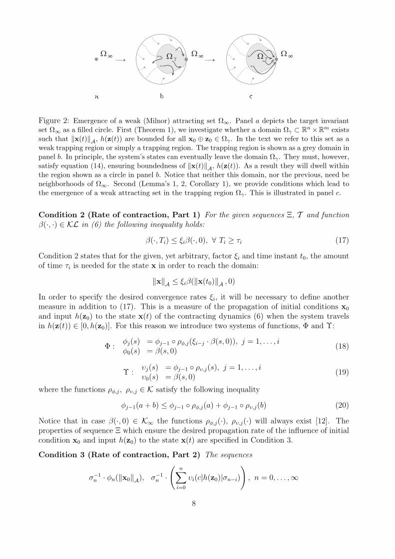
Figure 2: Emergence of a weak (Milnor) attracting set Ω∞. Panel a depicts the target invariantset Ω∞ as a filled circle. First (Theorem 1), we investigate whether a domain Ωγ ⊂ Rn×Rm existssuch that ‖x(t)‖A, h(z(t)) are bounded for all x0 ⊕ z0 ∈ Ωγ . In the text we refer to this set as aweak trapping region or simply a trapping region. The trapping region is shown as a grey domain inpanel b. In principle, the system’s states can eventually leave the domain Ωγ . They must, however,satisfy equation (14), ensuring boundedness of ‖x(t)‖A, h(z(t)). As a result they will dwell withinthe region shown as a circle in panel b. Notice that neither this domain, nor the previous, need beneighborhoods of Ω∞. Second (Lemma’s 1, 2, Corollary 1), we provide conditions which lead tothe emergence of a weak attracting set in the trapping region Ωγ . This is illustrated in panel c.
Condition 2 (Rate of contraction, Part 1) For the given sequences Ξ, T and functionβ(·, ·) ∈ KL in (6) the following inequality holds:
β(·, Ti) ≤ ξiβ(·, 0), ∀ Ti ≥ τi (17)
Condition 2 states that for the given, yet arbitrary, factor ξi and time instant t0, the amountof time τi is needed for the state x in order to reach the domain:
‖x‖A ≤ ξiβ(‖x(t0)‖A , 0)
In order to specify the desired convergence rates ξi, it will be necessary to define anothermeasure in addition to (17). This is a measure of the propagation of initial conditions x0
and input h(z0) to the state x(t) of the contracting dynamics (6) when the system travelsin h(z(t)) ∈ [0, h(z0)]. For this reason we introduce two systems of functions, Φ and Υ:
Φ :φj(s) = φj−1 ρφ,j(ξi−j · β(s, 0)), j = 1, . . . , iφ0(s) = β(s, 0)
(18)
Υ :υj(s) = φj−1 ρυ,j(s), j = 1, . . . , iυ0(s) = β(s, 0)
(19)
where the functions ρφ,j, ρυ,j ∈ K satisfy the following inequality
φj−1(a + b) ≤ φj−1 ρφ,j(a) + φj−1 ρυ,j(b) (20)
Notice that in case β(·, 0) ∈ K∞ the functions ρφ,j(·), ρυ,j(·) will always exist [12]. Theproperties of sequence Ξ which ensure the desired propagation rate of the influence of initialcondition x0 and input h(z0) to the state x(t) are specified in Condition 3.
Condition 3 (Rate of contraction, Part 2) The sequences
σ−1n · φn(‖x0‖A), σ−1
n ·(
n∑i=0
υi(c|h(z0)|σn−i)
), n = 0, . . . ,∞
8
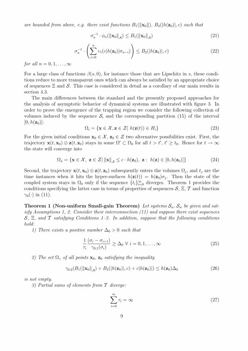
are bounded from above, e.g. there exist functions B1(‖x0‖), B2(|h(z0)|, c) such that
σ−1n · φn(‖x0‖A) ≤ B1(‖x0‖A) (21)
σ−1n ·
(n∑
i=0
υi(c|h(z0)|σn−i)
)≤ B2(|h(z0)|, c) (22)
for all n = 0, 1, . . . ,∞For a large class of functions β(s, 0), for instance those that are Lipschitz in s, these condi-tions reduce to more transparent ones which can always be satisfied by an appropriate choiceof sequences Ξ and S. This case is considered in detail as a corollary of our main results insection 4.3.
The main differences between the standard and the presently proposed approaches forthe analysis of asymptotic behavior of dynamical systems are illustrated with figure 3. Inorder to prove the emergence of the trapping region we consider the following collection ofvolumes induced by the sequence Si and the corresponding partition (15) of the interval[0, h(z0)]:
Ωi = x ∈ X , z ∈ Z| h(z(t)) ∈ Hi (23)
For the given initial conditions x0 ∈ X , z0 ∈ Z two alternative possibilities exist. First, thetrajectory x(t,x0) ⊕ z(t, z0) stays in some Ω′ ⊂ Ω0 for all t > t′, t′ ≥ t0. Hence for t → ∞the state will converge into
Ωa = x ∈ X , z ∈ Z| ‖x‖A ≤ c · h(z0), z : h(z) ∈ [0, h(z0)] (24)
Second, the trajectory x(t,x0)⊕ z(t, z0) subsequently enters the volumes Ωj, and tj are thetime instances when it hits the hyper-surfaces h(z(t)) = h(z0)σj. Then the state of thecoupled system stays in Ω0 only if the sequence ti∞i=0 diverges. Theorem 1 provides theconditions specifying the latter case in terms of properties of sequences S, Ξ, T and functionγ0(·) in (11).
Theorem 1 (Non-uniform Small-gain Theorem) Let systems Sa, Sw be given and sat-isfy Assumptions 1, 2. Consider their interconnection (11) and suppose there exist sequencesS, Ξ, and T satisfying Conditions 1–3. In addition, suppose that the following conditionshold:
1) There exists a positive number ∆0 > 0 such that
1
τi
(σi − σi+1)
γ0,1(σi)≥ ∆0 ∀ i = 0, 1, . . . ,∞ (25)
2) The set Ωγ of all points x0, z0 satisfying the inequality
γ0,2(B1(‖x0‖A) + B2(|h(z0)|, c) + c|h(z0)|) ≤ h(z0)∆0 (26)
is not empty.3) Partial sums of elements from T diverge:
∞∑i=0
τi = ∞ (27)
9
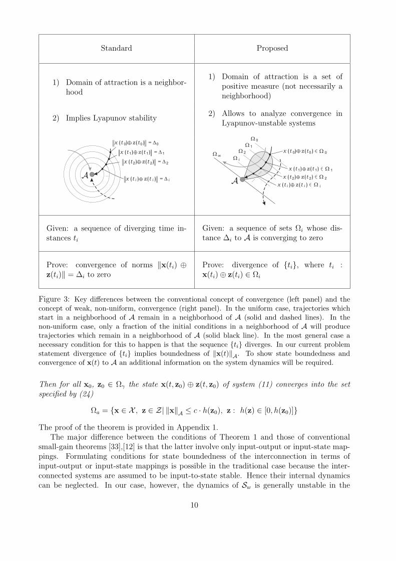
Standard Proposed
1) Domain of attraction is a neighbor-hood
1) Domain of attraction is a set ofpositive measure (not necessarily aneighborhood)
2) Implies Lyapunov stability2) Allows to analyze convergence in
Lyapunov-unstable systems
Given: a sequence of diverging time in-stances ti
Given: a sequence of sets Ωi whose dis-tance ∆i to A is converging to zero
Prove: convergence of norms ‖x(ti) ⊕z(ti)‖ = ∆i to zero
Prove: divergence of ti, where ti :x(ti)⊕ z(ti) ∈ Ωi
Figure 3: Key differences between the conventional concept of convergence (left panel) and theconcept of weak, non-uniform, convergence (right panel). In the uniform case, trajectories whichstart in a neighborhood of A remain in a neighborhood of A (solid and dashed lines). In thenon-uniform case, only a fraction of the initial conditions in a neighborhood of A will producetrajectories which remain in a neighborhood of A (solid black line). In the most general case anecessary condition for this to happen is that the sequence ti diverges. In our current problemstatement divergence of ti implies boundedness of ‖x(t)‖A. To show state boundedness andconvergence of x(t) to A an additional information on the system dynamics will be required.
Then for all x0, z0 ∈ Ωγ the state x(t, z0) ⊕ z(t, z0) of system (11) converges into the setspecified by (24)
Ωa = x ∈ X , z ∈ Z| ‖x‖A ≤ c · h(z0), z : h(z) ∈ [0, h(z0)]
The proof of the theorem is provided in Appendix 1.The major difference between the conditions of Theorem 1 and those of conventional
small-gain theorems [33],[12] is that the latter involve only input-output or input-state map-pings. Formulating conditions for state boundedness of the interconnection in terms ofinput-output or input-state mappings is possible in the traditional case because the inter-connected systems are assumed to be input-to-state stable. Hence their internal dynamicscan be neglected. In our case, however, the dynamics of Sw is generally unstable in the
10
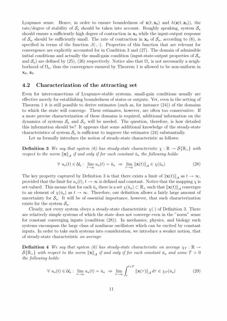
Lyapunov sense. Hence, in order to ensure boundedness of x(t,x0) and h(z(t, z0)), therate/degree of stability of Sa should be taken into account. Roughly speaking, system Sa
should ensure a sufficiently high degree of contraction in x0 while the input-output responseof Sw should be sufficiently small. The rate of contraction in x0 of Sa, according to (6), isspecified in terms of the function β(·, ·). Properties of this function that are relevant forconvergence are explicitly accounted for in Condition 3 and (27). The domain of admissibleinitial conditions and actually the small-gain condition (input-state-output properties of Sw
and Sa) are defined by (25), (26) respectively. Notice also that Ωγ is not necessarily a neigh-borhood of Ωa, thus the convergence ensured by Theorem 1 is allowed to be non-uniform inx0, z0.
4.2 Characterization of the attracting set
Even for interconnections of Lyapunov-stable systems, small-gain conditions usually areeffective merely for establishing boundedness of states or outputs. Yet, even in the setting ofTheorem 1 it is still possible to derive estimates (such as, for instance (24)) of the domainsto which the state will converge. These estimates, however, are often too conservative. Ifa more precise characterization of these domains is required, additional information on thedynamics of systems Sa and Sw will be needed. The question, therefore, is how detailedthis information should be? It appears that some additional knowledge of the steady-statecharacteristics of system Sa is sufficient to improve the estimates (24) substantially.
Let us formally introduce the notion of steady-state characteristic as follows:
Definition 3 We say that system (6) has steady-state characteristic χ : R → SR+ withrespect to the norm ‖x‖A if and only if for each constant ua the following holds:
∀ ua(t) ∈ Ua : limt→∞
ua(t) = ua ⇒ limt→∞
‖x(t)‖A ∈ χ(ua) (28)
The key property captured by Definition 3 is that there exists a limit of ‖x(t)‖A as t →∞,provided that the limit for ua(t), t →∞ is defined and constant. Notice that the mapping χ isset-valued. This means that for each ua there is a set χ(ua) ⊂ R+ such that ‖x(t)‖A convergesto an element of χ(ua) as t → ∞. Therefore, our definition allows a fairly large amount ofuncertainty for Sa. It will be of essential importance, however, that such characterizationexists for the system Sa.
Clearly, not every system obeys a steady-state characteristic χ(·) of Definition 3. Thereare relatively simple systems of which the state does not converge even in the ”norm” sensefor constant converging inputs (condition (28)). In mechanics, physics, and biology suchsystems encompass the large class of nonlinear oscillators which can be excited by constantinputs. In order to take such systems into consideration, we introduce a weaker notion, thatof steady-state characteristic on average:
Definition 4 We say that system (6) has steady-state characteristic on average χT : R →SR+ with respect to the norm ‖x‖A if and only if for each constant ua and some T > 0the following holds:
∀ ua(t) ∈ Ua : limt→∞
ua(t) = ua ⇒ limt→∞
∫ t+T
t
‖x(τ)‖A dτ ∈ χT (ua) (29)
11
Steady-state characterizations of system Sa allow to further specify the asymptotic behaviorof interconnection (11). These results are summarized in Lemmas 1 and 2 below.
Lemma 1 Let system (11) be given and h(z(t, z0)) be bounded for some x0, z0. Let, fur-thermore, system (6) have steady-state characteristic χ(·) : R→ SR+. Then the followinglimiting relations hold6
limt→∞
‖x(t,x0)‖A = 0, limt→∞
h(z(t, z0)) ∈ χ−1(0) (30)
As follows from Lemma 1, in case the steady-state characteristic of Sa is defined, the asymp-totic behavior of interconnection (11) is characterized by the zeroes of the steady-statemapping χ(·). For the steady-state characteristics on average a slightly modified conclusioncan be derived.
Lemma 2 Let system (11) be given, h(z(t, z0)) be bounded for some x0, z0, h(z(t, z0)) ∈[0, h(z0)], and system (6) have steady-state characteristic χT (·) : R → SR+ on average.Furthermore, let there exist a positive constant γ such that the function γ1(·) in (8) satisfiesthe following constraint:
γ1(s) ≥ γ · s, ∀s ∈ [0, s], s ∈ R+ : s > c · h(z0), (31)
In addition, suppose that χT (·) has no zeros in the positive domain, i.e. 0 /∈ χT (ua) for allua > 0. Then
limt→∞
‖x(t,x0)‖A = 0, limt→∞
h(z(t, z0)) = 0 (32)
An immediate outcome of Lemmas 1 and 2 is that in case the conditions of Theorem1 are satisfied and system (6) has steady-state characteristics χ(·) or χT (·) the domain ofconvergence Ωa becomes
Ωa = x ∈ X , z ∈ Z| ‖x‖A = 0, z : h(z) ∈ [0, h(z0)] (33)
It is possible, however, to improve estimate (33) further under additional hypotheses onsystem Sa and Sw dynamics. This result is formulated in the corollary below.
Corollary 1 Let system (11) be given and satisfy the assumptions of Theorem 1. Let, inaddition,
C1) the flow x(t,x0)⊕ z(t, z0) be generated by a system of autonomous differential equa-tions with locally Lipschitz right-hand side;
C2) subsystem Sw be practically integral-input-to-state stable:
‖z(τ)‖∞,[t0,t] ≤ Cz +
∫ t
0
γ1(uw(τ))dτ (34)
and let function h(·) ∈ C0 in (8)C3) system Sa have steady-state characteristic χ(·).
Then for all x0, z0 ∈ Ωγ the state of the interconnection converges to the set
Ωa = x ∈ X , z ∈ Z| ‖x‖A = 0, h(z) ∈ χ−1(0) (35)
6The symbol χ−1(0) in equation (30) denotes the set: χ−1(0) =⋃
ua∈R+ua : χ(ua) 3 0.
12
Figure 4: Control of the attracting set by means of the system’s steady-state characteristics
As follows from Corollary 1 zeros of the steady state characteristic of system Sa actually”controls” the domains to which the state of interconnection (11) might potentially converge.This is illustrated in Fig. 4. Notice also that in case condition C3 in Corollary 1 is replacedwith the alternative:
C3’) system Sa has a steady-state characteristic on average χT (·),then it is possible to show that the state converges to
Ωa = x ∈ X , z ∈ Z| ‖x‖A = 0, h(z) = 0 (36)
The proof follows straightforwardly from the proof of Corollary 1 and is therefore omitted.
4.3 Systems with contracting dynamics separable in space-time
In the previous sections we have presented convergence tests and estimates of the trappingregion, and also characterized the attracting sets of interconnection (11) under assumptionsof uniform asymptotic stability of Sa and input-output properties (8), (34) of system Sw.The conditions are given for rather general functions β(·, ·) ∈ KL in (6) and γ0(·), γ1(·) in(8). It appears, however, that these conditions can be substantially simplified if additionalproperties of β(·, ·) and γ0(·) are available. This information is, in particular, the separabilityof function β(·, ·) or, equivalently, the possibility of factorization:
β(‖x‖A , t) ≤ βx(‖x‖A) · βt(t), (37)
where βx(·) ∈ K and βt(·) ∈ C0 is strictly decreasing7 with
limt→∞
βt(t) = 0 (38)
In principle, as shown in [8], factorization (37) is achievable for a large class of uniformlyasymptotically stable systems under an appropriate coordinate transformation. An immedi-ate consequence of factorization (37) is that the elements of sequence Ξ in Condition 2 areindependent of ‖x(ti)‖A. As a result, verification of Conditions 2, 3 becomes easier. Themost interesting case, however, occurs when the function βx(·) in the factorization (37) isLipschitz. For this class of functions the conditions of Theorem 1 reduce to a single andeasily verifiable inequality. Let us consider this case in detail.
7If βt(·) is not strictly monotone, it can always be majorized by a strictly decreasing function
13
Without loss of generality, we assume that the state x(t) of system Sa satisfies thefollowing equation
‖x(t)‖A ≤ ‖x(t0)‖A · βt(t− t0) + c · ‖h(z(τ, z0))‖∞,[t0,t], (39)
where βt(0) is greater or equal to one. Given that βt(t) is strictly decreasing, the mappingβt : [0,∞] 7→ [0, βt(0)] is injective. Moreover βt(t) is continuous, then it is surjective and,therefore, bijective. In the other words there is a (continuous) mapping β−1
t : [0, βt(0)] 7→ R+:
β−1t βt(t) = t, ∀ t > 0 (40)
Conditions for emergence of the trapping region for interconnection (11) with dynamics ofsystem Sa governed by equation (39) are summarized below:
Corollary 2 Let the interconnection (11) be given, system Sa satisfy (39) and function γ0(·)in (8) be Lipschitz:
|γ0(s)| ≤ Dγ,0 · |s| (41)
and domain
Ωγ : Dγ,0 ≤(
β−1t
(d
κ
))−1κ− 1
κ
h(z0)
βt(0) ‖x0‖A + βt(0) · c · |h(z0)|(1 + κ
1−d
)+ c|h(z0)|
(42)
is not empty for some d < 1, κ > 1. Then for all initial conditions x0 z0 ∈ Ωγ the statex(t,x0) ⊕ z(t, z0) of interconnection (11) converges into the set Ωa specified by (24). If, inaddition, conditions C1)–C3) of Corollary 1 hold then the domain of convergence is given by(33).
A practically important consequence of this corollary concerns systems Sa which areexponentially stable:
‖x(t)‖A ≤ ‖x(t0)‖ADβ exp(−λt) + c · ‖h(z(t, z0))‖∞,[t0,t], λ > 0, Dβ ≥ 1 (43)
In this case the domain (42) of initial conditions ensuring convergence into Ωa is defined as
Dγ,0 ≤ maxκ>1, d∈(0,1)
−λ
(ln
d
κ
)−1κ− 1
κ
h(z0)
Dβ ‖x0‖A + Dβ · c · |h(z0)|(1 + κ
1−d
)+ c|h(z0)|
5 Discussion
In this section we discuss some practically relevant outcomes of the results of Theorem 1and Corollaries 1, 2 and their potential applications to problems of analysis of asymptoticbehavior in nonlinear dynamic systems.
First, in Subsection 5.1 we specify conditions for existence of a trapping region of nonzerovolume in Rn ⊕Rm in terms of the parameters of system (11) without invoking dependenceon x(t0), z(t0) as was done in Theorem 1. The resulting criterion has a form similar to thestandard small-gain conditions [33]. The differences and similarities between this new resultand standard small-gain theorems are illustrated with an example.
Second, in Subsection 5.2 we demonstrate how the results of our present contributioncan be applied to address the problem of output nonlinear identification for systems whichcannot be transformed into a canonic observer form or/and with nonlinear parametrization.
14
5.1 Relation to conventional small-gain theorems
Conditions specifying state boundedness formulated in Theorem 1 and Corollaries 1, 2 de-pend explicitly on initial conditions x(t0), z(t0). Such dependence is inevitable when theconvergence is allowed to be non-uniform. But if mere existence of a trapping region is askedfor, dependence on initial conditions may be removed from the statements of the results. Thenext corollary presents such modified conditions.
Corollary 3 Consider interconnection (11) where the system Sa satisfies inequality (39) andthe function γ0(·) obeys (41). Then there exists a set Ωγ of initial conditions correspondingto the trajectories converging to Ωa if the following condition is satisfied
Dγ,0 · c · G < 1, (44)
where
G = β−1t
(d
κ
)k
k − 1
(βt(0)
(1 +
κ
1− d
)+ 1
)
for some d ∈ (0, 1), κ ∈ (1,∞). In particular, Ωγ contains the following domain
‖x(t0)‖A ≤1
βt(0)
[1
Dγ,0
(β−1
t
(d
κ
))−1k − 1
k− c
(βt(0)
(1 +
κ
1− d
)+ 1
)]h(z(t0)).
In case the function h(z) in (11) is continuous, the volume of the set Ωγ is nonzero inRn ⊕ Rm.
Notice that in case the dynamics of the contracting subsystem Sa is exponentially stable,i.e. it satisfies inequality (43), the term G in condition (44) reduces to
G =1
λ· ln
(κ
d
) k
k − 1
(Dβ
(1 +
κ
1− d
)+ 1
)(45)
For Dβ = 1 the minimal value of G in (45) can be estimated as
G∗ =1
λ· min
d∈(0,1), κ∈(1,∞)ln
(κ
d
) k
k − 1
(2 +
κ
1− d
)≈ 15.6886
λ<
16
λ, (46)
which leads to an even more simple formulation of (45):
Dγ,0 · c
λ≤ 1
16
Corollary 3 provides an explicit and easy-to-check condition for existence of a trappingregion in the state space of a class of Lyapunov unstable systems. In addition, it allows tospecify explicitly points x(t0), z(t0) which belong to the emergent trapping region. Noticealso that the existence condition, inequality (44), has the flavor of conventional small-gainconstraints. Yet, it is substantially different from these classical results. This is because theinput-output gain for the wandering subsystem, Sw, may not be finite or need not even bedefined.
15
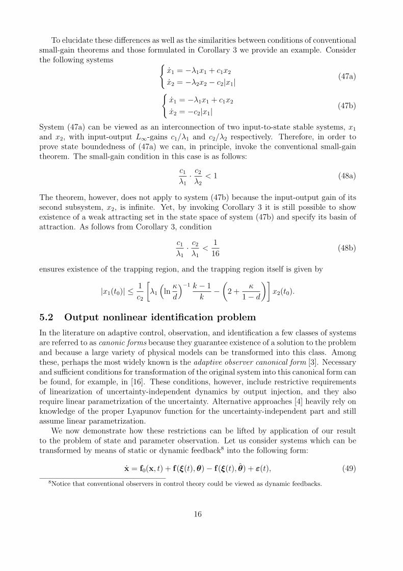
To elucidate these differences as well as the similarities between conditions of conventionalsmall-gain theorems and those formulated in Corollary 3 we provide an example. Considerthe following systems
x1 = −λ1x1 + c1x2
x2 = −λ2x2 − c2|x1|(47a)
x1 = −λ1x1 + c1x2
x2 = −c2|x1|(47b)
System (47a) can be viewed as an interconnection of two input-to-state stable systems, x1
and x2, with input-output L∞-gains c1/λ1 and c2/λ2 respectively. Therefore, in order toprove state boundedness of (47a) we can, in principle, invoke the conventional small-gaintheorem. The small-gain condition in this case is as follows:
c1
λ1
· c2
λ2
< 1 (48a)
The theorem, however, does not apply to system (47b) because the input-output gain of itssecond subsystem, x2, is infinite. Yet, by invoking Corollary 3 it is still possible to showexistence of a weak attracting set in the state space of system (47b) and specify its basin ofattraction. As follows from Corollary 3, condition
c1
λ1
· c2
λ1
<1
16(48b)
ensures existence of the trapping region, and the trapping region itself is given by
|x1(t0)| ≤ 1
c2
[λ1
(ln
κ
d
)−1 k − 1
k−
(2 +
κ
1− d
)]x2(t0).
5.2 Output nonlinear identification problem
In the literature on adaptive control, observation, and identification a few classes of systemsare referred to as canonic forms because they guarantee existence of a solution to the problemand because a large variety of physical models can be transformed into this class. Amongthese, perhaps the most widely known is the adaptive observer canonical form [3]. Necessaryand sufficient conditions for transformation of the original system into this canonical form canbe found, for example, in [16]. These conditions, however, include restrictive requirementsof linearization of uncertainty-independent dynamics by output injection, and they alsorequire linear parametrization of the uncertainty. Alternative approaches [4] heavily rely onknowledge of the proper Lyapunov function for the uncertainty-independent part and stillassume linear parametrization.
We now demonstrate how these restrictions can be lifted by application of our resultto the problem of state and parameter observation. Let us consider systems which can betransformed by means of static or dynamic feedback8 into the following form:
x = f0(x, t) + f(ξ(t), θ)− f(ξ(t), θ) + ε(t), (49)
8Notice that conventional observers in control theory could be viewed as dynamic feedbacks.
16
whereε(t) ∈ Lm
∞[t0,∞], ‖ε(τ)‖∞,[t0,t] ≤ ∆ε
is an external perturbation with known ∆ε, and x ∈ Rn. The function ξ : R+ → Rξ
is a function of time, which possibly includes available measurements of the state, andθ, θ ∈ Ωθ ⊂ Rd are the unknown and estimated parameters of function the f(·), respectively,and the set Ωθ is bounded. We assume that the function f(ξ(t),θ) is locally bounded in θuniformly in ξ:
‖f(ξ(t),θ)− f(ξ(t), θ)‖ ≤ Df‖θ − θ‖+ ∆f
and the values of Df ∈ R+, ∆f are available. The function f0(·) in (49) is assumed to satisfythe following condition.
Assumption 3 The systemx = f0(x, t) + u(t) (50)
is forward-complete. Furthermore, for all u(t) such that
‖u(t)‖∞,[t0,t] ≤ ∆u + ‖u0(τ)‖∞,[t0,t], ∆u ∈ R+
there exists a bounded set A, c > 0 and a function ∆ : R+ → R+ satisfying the followinginequality
‖x(t)‖A∆(∆u)≤ β(t− t0) ‖x(t0)‖A∆(∆u)
+ c‖u0(τ)‖∞,[t0,t]
where β(·) : R+ → R+, limt→∞ β(t) = 0 is a strictly decreasing function
Consider the following auxiliary system
λ = S(λ), λ(t0) = λ0 ∈ Ωλ ⊂ Rλ (51)
where Ωλ ⊂ Rn is bounded and S(λ) is locally Lipschitz. Furthermore, suppose that thefollowing assumption holds for system (51).
Assumption 4 System (51) is Poisson stable in Ωλ that is
∀ λ′ ∈ Ωλ, t′ ∈ R+ ⇒ ∃t′′ > t : ‖λ(t′′, λ′)− λ′‖ ≤ ε,
where ε is an arbitrary small positive constant. Moreover, the trajectory λ(t,λ0) is dense inΩλ:
∀λ′ ∈ Ωλ, ε ∈ R>0 ⇒ ∃ t ∈ R+ : ‖λ′ − λ(t, λ0)‖ < ε
Now we are ready to formulate the following statement
Corollary 4 Consider system (49) and suppose that the following conditions holdC4) the vector-field f0(x, t) in (49) satisfies Assumption 3;C5) there exists a (known) system (51) satisfying Assumption 4;C6) there exists a locally Lipschitz η : Rλ → Rd:
‖η(λ′)− η(λ′′)‖ ≤ Dη‖λ′ − λ′′‖such that the set η(Ωλ) is dense in Ωθ;
C7) system (49) has steady-state characteristic with respect to the norm
‖·‖A∆(M), M = 2∆f + ∆ε + δ
17
and input θ, where δ is some positive (arbitrary small) constant.Consider the following interconnection of (49), (51):
x = f0(x, t) + f(ξ(t),θ)− f(ξ(t), θ) + ε(t)
θ = η(λ)
λ = γ ‖x(t)‖A∆(M)S(λ),
(52)
where γ > 0 satisfies the following inequality
γ ≤(
β−1t
(d
κ
))−1κ− 1
κ
1
Dλ
(βt(0)
(1 + κ
1−d
)+ 1
)
Dλ = c ·Df ·Dη · maxλ∈Ωλ
‖S(λ)‖(53)
for some d ∈ (0, 1), κ ∈ (1,∞). Then, for λ(t0) = λ0, some θ′ ∈ Ωθ and all x(t0) = x0 ∈ Rn
the following holds
limt→∞
‖x(t)‖A∆(M)= 0, lim
t→∞θ(t) = θ′ ∈ Ωθ (54)
Notice that, as has been pointed out in the previous section, in case the dynamics of (50) isexponentially stable with rate of convergence equal to ρ and β(0) = Dβ, condition (53) willhave the following form
γ ≤ −ρ
(ln
d
κ
)−1κ− 1
κ
1
Dλ
(Dβ
(1 + κ
1−d
)+ 1
)
According to Corollary 4, for the rather general class of systems (49) it is possible todesign an estimator θ(t) which guarantees that not only the ”error” vector x(t) reaches aneighborhood of the origin, but also that the estimates θ(t) converge to some θ′ in Ωθ. Boththese facts, together with additional nonlinear persistent excitation conditions [6],[27]
∃T > 0, ρ ∈ K : ∀ T = [t, t+T ], t ∈ R+ ⇒ ∃τ ∈ T : |f(ξ(τ),θ)− f(ξ(τ),θ′)| ≥ ρ(‖θ−θ′‖),in principle allow us to estimate the domain of convergence for θ(t).
Concluding this section we mention that statements of Theorem 1 and Corollaries 1–4constitute additional theoretical tools for the analysis of asymptotic behavior of systems incascaded form. In particular they are complementary to the results of [1] where asymptoticstability of the following type of systems
x = f(x),
z = q(x, z), f : Rn → Rn, q : Rn × Rm → Rm
was considered under assumption that the x-subsystem is globally asymptotically stable andthe z-subsystem is integral input-to-state stable. In contrast to this, our results apply toestablishing asymptotic convergence for systems with the following structure
x = f(x, z),
z = q(x, z), f : Rn × Rm → Rn
where the x-subsystem is input-to-state stable, and the z-subsystem could be practicallyintegral input-to-state stable (see Corollary 1), although in general no stability assumptionsare imposed on it.
18

6 Examples
In this section we provide two examples of parameter identification in nonlinearly parame-terized systems that cannot be transformed into the canonical adaptive observer form.
The first example is merely an academical illustration of Corollary 4, where only oneparameter is unknown and the system itself is a first-order differential equation. The secondexample illustrates a possible application of our results to the problem of identifying thedynamics in living cells.
Example 1. Consider the following system
x = −kx + sin(xθ + θ) + u, k > 0, θ ∈ [−a, a] (55)
where θ is an unknown parameter and u is the control input. Without loss of generality welet a = 1, k = 1. The problem is to estimate the parameter θ from measurements of x andsteer the system to the origin. Clearly, the choice u = − sin(xθ + θ) transforms (55) into
x = −kx + sin(xθ + θ)− sin(xθ + θ) (56)
which satisfies Assumption 3. Moreover, the system
λ1 = λ1
λ2 = −λ2, λ21(t0) + λ2
2(t0) = 1
with mapping η = (1, 0)T λ satisfies Assumption 4 and therefore
λ1 = γ|x|λ1
λ2 = −γ|x|λ2, λ21(t0) + λ2
2(t0) = 1(57)
would be a candidate for the control and parameter estimation algorithm. According toCorollary 4, the goal will be reached if the parameter γ in (57) obeys the following constraint
γ ≤ −ρ
(ln
d
κ
)−1κ− 1
κ
1
Dλ
(Dβ
(1 + κ
1−d
)+ 1
) , ρ = k = 1, Dβ = 1, Dλ = 1
for some d ∈ (0, 1), κ ∈ (1,∞). Hence, choosing, for example, d = 0.5, κ = 2 we obtain thatchoice
0 < γ < − ln
(0.5
2
)−11
2· 1
6= 0.0601
suffices to ensure thatlimt→∞
x(t) = 0, limt→∞
θ(t) = θ
We simulated system (56), (57) with θ = 0.3, γ = 0.05 and initial conditions x(t0)randomly distributed in the interval [−1, 1]. Results of the simulation are illustrated withFigure 5, where the phase plots of system (56), (57) as well as the trajectories of θ(t) aregiven.
Example 2. Consider the problem of modelling electrical activity in biological cells fromthe input-output data in current clamp experiments. The simplest mathematical model,which captures a fairly large variety of phenomena like periodic bursting in response to
19
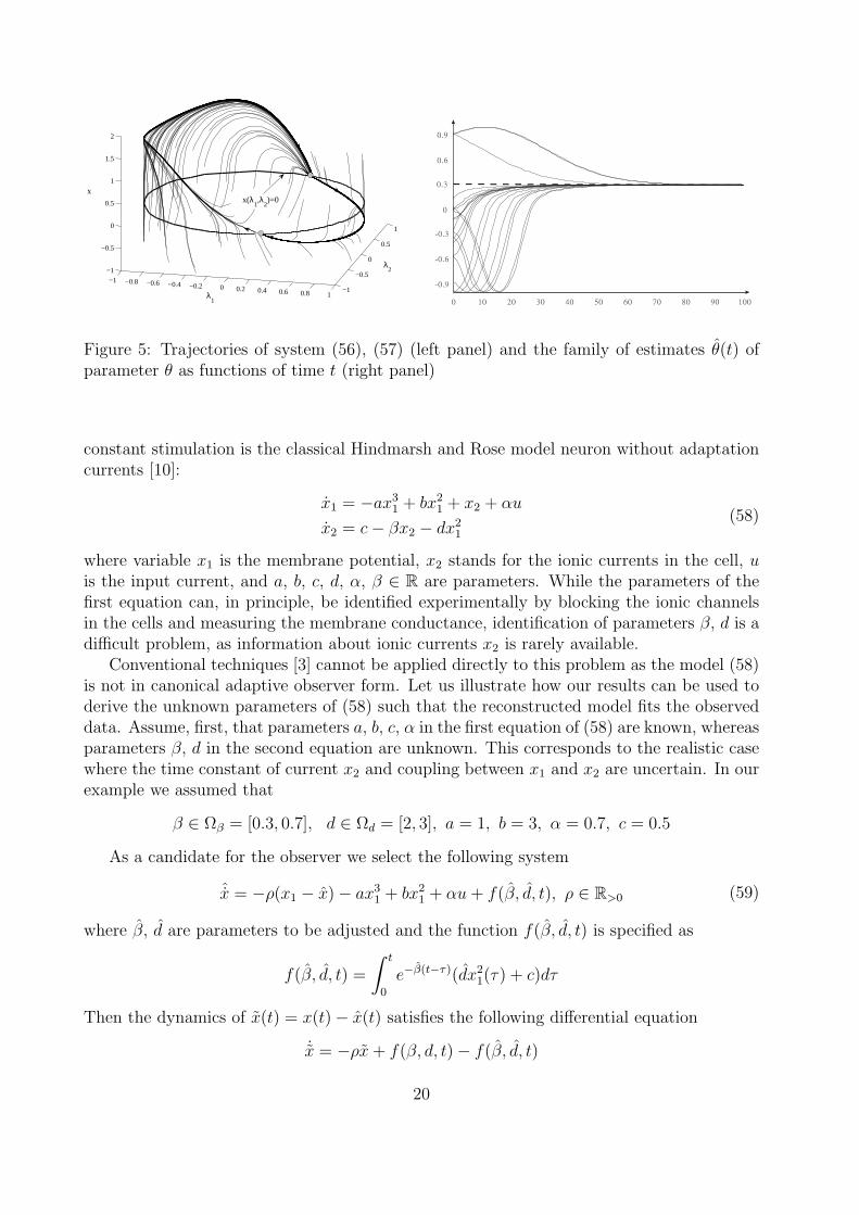
−1 −0.8 −0.6 −0.4 −0.2 0 0.2 0.4 0.6 0.8 1−1
−0.5
0
0.5
1
−1
−0.5
0
0.5
1
1.5
2
x
λ1
λ2
x(λ1,λ
2)=0
Figure 5: Trajectories of system (56), (57) (left panel) and the family of estimates θ(t) ofparameter θ as functions of time t (right panel)
constant stimulation is the classical Hindmarsh and Rose model neuron without adaptationcurrents [10]:
x1 = −ax31 + bx2
1 + x2 + αu
x2 = c− βx2 − dx21
(58)
where variable x1 is the membrane potential, x2 stands for the ionic currents in the cell, uis the input current, and a, b, c, d, α, β ∈ R are parameters. While the parameters of thefirst equation can, in principle, be identified experimentally by blocking the ionic channelsin the cells and measuring the membrane conductance, identification of parameters β, d is adifficult problem, as information about ionic currents x2 is rarely available.
Conventional techniques [3] cannot be applied directly to this problem as the model (58)is not in canonical adaptive observer form. Let us illustrate how our results can be used toderive the unknown parameters of (58) such that the reconstructed model fits the observeddata. Assume, first, that parameters a, b, c, α in the first equation of (58) are known, whereasparameters β, d in the second equation are unknown. This corresponds to the realistic casewhere the time constant of current x2 and coupling between x1 and x2 are uncertain. In ourexample we assumed that
β ∈ Ωβ = [0.3, 0.7], d ∈ Ωd = [2, 3], a = 1, b = 3, α = 0.7, c = 0.5
As a candidate for the observer we select the following system
ˆx = −ρ(x1 − x)− ax31 + bx2
1 + αu + f(β, d, t), ρ ∈ R>0 (59)
where β, d are parameters to be adjusted and the function f(β, d, t) is specified as
f(β, d, t) =
∫ t
0
e−β(t−τ)(dx21(τ) + c)dτ
Then the dynamics of x(t) = x(t)− x(t) satisfies the following differential equation
˙x = −ρx + f(β, d, t)− f(β, d, t)
20
The function f(β, d, t) satisfies the following inequality
|f(β, d, t)− f(β, d, t)| ≤ |f(β, d, t)− f(β, d, t)|+ |f(β, d, t)− f(β, d, t)|≤ Df,β|β − β|+ Df,d|d− d|+ ε(t),
where ε(t) is an exponentially decaying term, and
Df,β = maxβ,β∈Ωβ , d∈Ωd
1
ββ(d‖x1(τ)‖∞,[t0,∞] + c)
, Df,d = max
β∈Ωβ
1
β‖x1(τ)‖∞,[t0,∞]
(60)
Furthermore, Assumption 3 is satisfied for system
˙x = −ρx + υ(t), (61)
with
∆(∆u) =∆u
ρ.
In particular, for all υ(t) : ‖υ(τ)‖∞,[t0,t] ≤ ∆u +‖υ0(τ)‖∞,[t0,t] the following inequality holds:
‖x(t)‖∆(∆u) ≤ e−ρ(t−t0)‖x(t0)‖∆(∆u) +1
ρ‖υ0(τ)‖∞,[t0,t]. (62)
To see this consider the general solution of (61):
x(t) = e−ρ(t−t0)x(t0) + e−ρt
∫ t
t0
eρτυ(τ)dτ
and derive an estimate of |x(t)|. This estimate has the following form:
|x(t)| ≤ e−ρ(t−t0)|x(t0)|+ 1
ρ
(1− e−ρ(t−t0)
) ‖υ(τ)‖∞,[t0,t]
≤ e−ρ(t−t0)
(|x(t0)| − 1
ρ∆u
)+
1
ρ
(‖υ0(τ)‖∞,[t0,t] + ∆u
)
≤ e−ρ(t−t0)‖x(t0)‖∆(∆u) +1
ρ
(‖υ0(τ)‖∞,[t0,t] + ∆u
)
Hence
|x(t)| − 1
ρ∆u ≤ e−ρ(t−t0)‖x(t0)‖∆(∆u) +
1
ρ‖υ0(τ)‖∞,[t0,t],
which automatically implies (62).Let us define subsystem (51). Consider the following system of differential equations
λ1 = λ2
λ2 = −ω21λ1
λ3 = λ4
λ4 = −ω22λ3, λ0 = (1, 0, 1, 0)T
(63)
21
where Ωλ is the ω-limit set of the point λ0, and ω1, ω2 ∈ R. System (63), therefore, satisfiesAssumption 4. Given that domains Ωβ, Ωd are known, select
η : Rn → R2, η = (η1(λ), η2(λ))
β = η1(λ) =1
2
(2 arcsin(λ1)
π+ 1
)· 0.4 + 0.3, d = η2(λ) =
1
2
(2 arcsin(λ3)
π+ 1
)+ 2
(64)
Choosingω1
ω2
= π
we ensure that η(Ωλ) is dense in Ωβ × Ωd. Given that β, d are bounded and β ≥ 0.3, Df,β
and Df,d in (60) are also bounded because for the given range of parameters signal x1(t) isalways bounded. Hence, according to Corollary 4, interconnection of (59), (64) and
λ1 = γ‖x(t)‖∆(δ) · λ2
λ2 = −γ‖x(t)‖∆(δ) · ω21λ1
λ3 = γ‖x(t)‖∆(δ) · λ4
λ4 = −γ‖x(t)‖∆(δ) · ω22λ3, λ0 = (1, 0, 1, 0)T
with arbitrary small δ > 0 and properly chosen γ > 0 ensures that
limt→∞
‖x(t)‖∆(δ) = 0, limt→∞
β(t) = β′ ∈ Ωβ, limt→∞
d(t) = d′ ∈ Ωd
This in turn implies a successful fit of the model to the observations.We simulated the system with ρ = 10 and γ = 3 · 10−4 for β = 0.5, d = 2.5. The
results of the simulations are provided in figure 6. It can be seen from this figure that thereconstruction is successful and the parameters converge into a small neighborhood of theactual values.
7 Conclusion
We proposed tools for the analysis of asymptotic behavior of a class of dynamical systems. Inparticular, we consider an interconnection of an input-to-state stable system with an unstableor integrally input-to-state dynamics. Our results allow to address a variety of problems inwhich convergence may not be unform with respect to initial conditions. It is necessaryto notice that the proposed method does not require complete knowledge of the dynamicalsystems in question. Only qualitative information like, for instance, characterization ofinput-to-state stability of is necessary for application of our results. We demonstrated howour analysis can be used in the problems of synthesis and design – in particular to problemsof nonlinear regulation and parameter identification of nonlinear parameterized systems.The examples show the relevance of our approach in those domains where application of thestandard techniques is either not possible or too complicated.
8 Acknowledgment
The authors are thankful to Peter Jurica and Tatiana Tyukina for their enthusiastic helpand comments during the preparation of this manuscript.
22

Figure 6: Left panel – trajectories x1(t), x2(t) of system (58) plotted for the nominal valuesof parameters β = 0.5, d = 2.5 (model), and for the values β = β(t0 + T ), d = d(t0 + T ),where T is the total simulation time (reconstruction). Input u(t) is a rectangular impulsewith amplitude 0.7 starting at t = 100 and ending at t = 300. Right panel – searchingdynamics in the bounded parameter space (a segment of the trajectory β(t), d(t) towardsthe end of the simulation).
9 Appendix
Proof of Theorem 1. Let the conditions of the theorem be satisfied for given t0 ∈ R+:x(t0) = x0, z(t0) = z0. Notice that in this case h(z0) ≥ 0, otherwise requirement (26) willbe violated. Consider the sequence (23) of volumes Ωi induced by S:
Ωi = x ∈ X , z ∈ Z| h(z(t)) ∈ HiTo prove the theorem we show that 0 ≤ h(z(t)) ≤ h(z0) for all t ≥ t0. For the given partition(23) we consider two alternatives.
First, in the degenerative case, the state x(t)⊕z(t) enters some Ωj, j ≥ 0 and stays therefor all t ≥ t0 which automatically guarantees that 0 ≤ |h(z)| ≤ h(z0). Then, according to(6) the trajectory x(t) satisfies the following inequality:
‖x(t)‖A ≤ β(‖x0‖A , t− t0) + c‖h(z(t))‖∞,[t0,t] ≤ β(‖x0‖A , t− t0) + c|h(z0)| (65)
Taking into account that β(·, ·) ∈ KL we can conclude that (65) implies that
lim supt→∞
‖x(t)‖A = c|h(z0)| (66)
Therefore the statements of the theorem hold.Let us consider the second alternative, where the state x(t)⊕ z(t) does not belong to Ωj
for all t ≥ t0. Given that h(z(t)) is monotone and non-increasing in t, this implies that thereexists an ordered sequence of time instants tj:
t0 > t1 > t2 · · · tj > tj+1 · · · (67)
such thath(z(ti)) = σih(z0) (68)
23
Hence in order to prove the theorem we must show that the sequence ti∞i=0 does notconverge. In other words, the boundary σ∞h(z0) = 0 will not be reached in finite time.
In order to do this let us estimate the upper bounds for the following differences
Ti = ti+1 − ti
Taking into account inequality (8) and the fact that γ0(·) ∈ Ke we can derive that
h(z(ti))− h(z(ti+1)) ≤ Ti maxτ∈[ti,ti+1]
γ0(‖x(τ)‖A) ≤ Tiγ0(‖x(τ)‖A∞,[ti,ti+1]) (69)
According to the definition of ti in (68) and noticing that the sequence S is strictly decreasingwe have
h(z(ti))− h(z(ti+1)) = (σi − σi+1)h(z0) > 0
Hence h(z0) > 0 implies that γ0(‖x(τ)‖A∞,[ti,ti+1]) > 0 and, therefore, (69) results in the
following estimate of Ti
Ti ≥ h(z(ti))− h(z(ti+1))
γ0(‖x(τ)‖A∞,[ti,ti+1])
=h(z0)(σi − σi+1)
γ0(‖x(τ)‖A∞,[ti,ti+1])
(70)
Taking into account that h(z(t)) is non-increasing over [ti, ti+1] and using (6) we can boundthe norm ‖x(τ)‖A∞,[ti,ti+1]
as follows
‖x(τ)‖A∞,[ti,ti+1]≤ β(‖x(ti)‖A , 0) + c‖h(z(τ))‖∞,[ti,ti+1] ≤ β(‖x(ti)‖A , 0) + c · σih(z0) (71)
Hence, combining (70) and (71) we obtain that
Ti ≥ h(z0)(σi − σi+1)
γ0(σi(σ−1i β(‖x(ti)‖A , 0) + c · h(z0)))
Then, using property (10) of function γ0 we can derive that
Ti ≥ h(z0)(σi − σi+1)
γ0,1(σi)
1
γ0,2(σ−1i β(‖x(ti)‖A , 0) + c · h(z0)))
(72)
Taking into account condition (27) of the theorem, the theorem will be proven if we assurethat
Ti ≥ τi (73)
for all i = 0, 1, 2, . . . ,∞. We prove this claim by induction with respect to the index i =0, 1, . . . ,∞. We start with i = 0, and then show that for all i > 0 the following implicationholds
Ti ≥ τi ⇒ Ti+1 ≥ τi+1 (74)
Let us prove that (73) holds for i = 0. To this purpose consider the term (σi − σi+1)/γ0,1(σi).As follows immediately from the conditions of the theorem, equation (25), we have that
σi − σi+1
γ0,1(σi)≥ τi∆0 ∀ i ≥ 0 (75)
In particularσ0 − σ1
γ0,1(σ0)≥ τ0∆0
24
Therefore, inequality (72) reduces to
T0 ≥ τ0∆0h(z0)
γ0,2(σ−10 β(‖x(t0)‖A , 0) + c · h(z0))
(76)
Moreover, taking into account Condition 3 and (18), (19) we can derive the following esti-mate:
σ−10 β(‖x(t0)‖A , 0) ≤ σ−1
0 φ0(‖x(t0)‖A) + σ−10 υ0(c · |h(z0)|σ0) ≤ B1(‖x0‖A) + B2(|h(z0)|, c)
According to the theorem conditions x0 and z0 satisfy inequality (26). This in turn impliesthat
γ0,2(σ−10 β(‖x(t0)‖A , 0) + c · h(z0)) ≤ γ0,2(B1(‖x0‖A) + B2(|h(z0)|, c) + c · h(z0)) ≤ ∆0 · h(z0)
(77)Combining (76) and (77) we obtain the desired inequality
T0 ≥ τ0∆0h(z0)
γ0,2(σ−10 β(‖x(t0)‖A , 0) + c · h(z0))
≥ τ0∆0h(z0)
∆0h(z0)= τ0
Thus the basis of induction is proven.Let us assume that (73) holds for all i = 0, . . . , n, n ≥ 0. We shall prove now that
implication (74) holds for i = n + 1. Consider the term β(‖x(tn+1)‖A , 0):
β(‖x(tn+1)‖A , 0) ≤ β(β(‖x(tn)‖A , Tn) + c‖h(z(τ))‖∞,[tn,tn+1], 0)
≤ β(β(‖x(tn)‖A , Tn) + c · σn · h(z0), 0)
Taking into account Condition 2 (specifically, inequality (17)) and (18)–(20) we can derivethat
β(‖x(tn+1)‖A , 0) ≤ β(ξn ·β(‖x(tn)‖A), 0)+c ·σn ·h(z0), 0) ≤ φ1(‖x(tn)‖A)+υ1(c · |h(z)0| ·σn)(78)
Notice that, according to the inductive hypothesis (Ti ≥ τi), the following holds
‖x(ti+1)‖A ≤ β(‖x(ti)‖A , Ti) + c · σi · h(z0) ≤ ξiβ(‖x(ti)‖A , 0) + c · σi · h(z0) (79)
for all i = 0, . . . , n. Then (78), (79), (18)–(20) imply that
β(‖x(tn+1)‖A , 0) ≤ φ1(ξiβ(‖x(tn−1)‖A , 0) + c · σn−1 · h(z0)) + υ1(c · |h(z)0| · σn)
≤ φ2(‖x(tn−1)‖A) + υ2(c · |h(z0)| · σn−1) + υ1(c · |h(z0)| · σn)
≤ φn+1(‖x0‖A) +n+1∑i=1
υi(c · |h(z0)|σn+1−i) ≤ φn+1(‖x0‖A) +n+1∑i=0
υi(c · |h(z0)|σn+1−i)
(80)
According to Condition 3, term
σ−1n+1
(φn+1(‖x0‖A) +
n+1∑i=0
υi(c · |h(z0)|σn+1−i)
)
is bounded from above by the sum
B1(‖x0‖A) + B2(|h(z0)|, c)
25
Therefore, monotonicity of γ0,2, estimate (80), and inequality (26) lead to the followinginequality
γ0,2(σ−1n+1β(‖x(tn+1‖A), 0)+ c ·h(z0)) ≤ γ0,2(B1(‖x0‖A)+B2(|h(z0)|, c)+ c ·h(z0)) ≤ h(z0)∆0
Hence, according to (72), (75) we have:
Tn+1 ≥ (σn+1 − σn+2)
γ0,1(σn+1)
h(z0)
γ0,2(σ−1n+1β(‖x(tn+1)‖A , 0) + c · h(z0))
≥ τn+1∆0h(z0)
∆0h(z0)= τn+1
Thus implication (74) is proven. This implies that h(z(t)) ∈ [0, h(z0)] for all t ≥ t0 and,consequently, that (66) holds. The theorem is proven.
Proof of Lemma 1. As follows from the assumptions, h(z(t, z0)) is bounded. Assume itbelongs to the following interval [a, h(z0)], a ≤ h(z0). Therefore, as follows from (8) we canconclude that
0 ≤∫ ∞
t0
γ1(‖x(τ,x0)‖A)dτ ≤ h(z0)− h(z(t, z0)) ≤ ∞ (81)
On the other hand, taking into account that h(z(t, z0)) is bounded and monotone in t(every subsequence of which is this is again monotone) and applying the Bolzano-Weierstrasstheorem we can conclude that h(z(t, z0)) converges in [a, h(z0)]. In particular, there existsh ∈ [a, h(z0)] such that
limt→∞
h(z(t, z0)) = h (82)
According to the lemma assumptions, system Sa has steady-state characteristics. This meansthat there exists a constant x ∈ R+ such that
limt→∞
‖x(t,x0)‖A = x (83)
Suppose that x > 0. Then it follows from (83) that there exists time instant t1 < ∞ andsome constant 0 < δ < x such that
‖x(t)‖A ≥ δ ∀t ≥ t1
Hence using (81) and noticing that γ1 ∈ Ke we obtain
∞ > h(z0)− h(z0) ≥ limT→∞
∫ T
t1
γ1(δ)dτ = ∞
Thus we obtained a contradiction. Hence, x = 0 and, consequently,
limt→∞
‖x(t)‖A = 0
Then, according to the notion of steady-state characteristic in Definition 3 this is onlypossible if h ∈ χ−1(0). The lemma is proven.
Proof of Lemma 2. Analogously to the proof of Lemma 1 we notice that (81) holds. This,however, implies that for any constant and positive T the following limit
limt→∞
∫ t+T
t
γ1(‖x(τ)‖A)dτ
26
exists and equals zero. Furthermore, h(z(t, z0)) ∈ [0, h(z0)] for all t ≥ t0. Hence, there existsa time instant t′ such that
‖x(t)‖A ≤ c · h(z0) + ε, ∀ t ≥ t′,
where ε > 0 is arbitrary small. Then taking into account (31) we can conclude that
limt→∞
∫ t+T
t
γ1(‖x(τ)‖A)dτ ≥ γ
∫ t+T
t
‖x(τ)‖A dτ = 0 (84)
Given that (82) holds, system (6) has the steady-state characteristic on average and thatχT (·) has no zeros in the positive domain, limiting relation (84) is possible only if h = 0.Then, according to (6), limt→∞ ‖x(t)‖A = 0. The lemma is proven.
Proof of Corollary 1. As follows from Theorem 1, state x(t,x0) ⊕ z(t, z0) converges tothe set Ωa specified by (24). Hence h(z(t, z0)) is bounded. Then, according to (8), estimate(81) holds. This, in combination with condition (34), implies that z(t, z0) is bounded. Inother words
x(t,x0)⊕ z(t, z0) ∈ Ω′ ∀ t ≥ t0
where Ω′ is a bounded subset in Rn × Rm. Applying the Bolzano-Weierstrass theorem wecan conclude that for every point x0 ⊕ z0 ∈ Ωγ there is an ω-limit set ω(x0 ⊕ z0) ⊆ Ω′
(non-empty).As follows from C3) and Lemma 1 the following holds:
limt→∞
h(z(t, z0)) ∈ χ−1(0)
Therefore, given that h(·) ∈ C0, we can obtain that
limti→∞
h(z(ti, z0)) = h( limti→∞
z(ti, z0)) = h(ωz(x0 ⊕ z0)) ∈ χ−1(0)
In other words:
ωz(x0 ⊕ z0) ⊆ Ωh = x ∈ Rn, z ∈ Rm| h(z) ∈ χ−1(0)
Moreoverωx(x0 ⊕ z0) ⊆ Ωa = x ∈ Rn, z ∈ Rm| ‖x‖A = 0
According to assumption C1, the flow x(t,x0) ⊕ z(t, z0) is generated by a system of au-tonomous differential equations with locally Lipschitz right-hand side. Then, as follows from[13] (Lemma 4.1, page 127)
limt→∞
dist(x(t,x0)⊕ z(t, z0), ω(x0 ⊕ z0)) = 0
Noticing that
dist(x(t,x0)⊕ z(t, z0), ω(x0 ⊕ z0)) ≥ dist(x(t,x0), Ωa) + dist(z(t, z0), Ωh)
we can finally obtain that
limt→∞
dist(x(t,x0), Ωa) = 0, limt→∞
dist(z(t, z0), Ωh) = 0
27
The corollary is proven.
Proof of Corollary 2. As follows from Theorem 1, the corollary will be proven if Condi-tions 1 – 3 are satisfied and also (25), (26), and (27) hold. In order to satisfy Condition 1we select the following sequence S:
S = σi∞i=0, σi =1
κi, κ ∈ R+, κ > 1 (85)
Let us chose sequences T and Ξ as follows:
T = τi∞i=0, τi = τ ∗, (86)
Ξ = ξi∞i=0, ξi = ξ∗, (87)
where τ ∗, ξ∗ are positive constants yet to be defined. Notice that choosing T as in (86)automatically fulfills condition (27) of Theorem 1. On the other hand, taking into account(17), (39) and that βt(t) is monotonically decreasing in t, this choice defines a constant ξ∗
as follows:βt(τ
∗) ≤ ξ∗βt(0) < βt(0), 0 ≤ ξ∗ < 1 (88)
Given that the inverse β−1t exists, (40), this choice is always possible. In particular, (88) will
be satisfied for the following values of τ ∗:
τ ∗ ≥ β−1t (ξ∗βt(0)) (89)
Let us now find the values for τ ∗ and ξ∗ such that Condition 3 is also satisfied. To thispurpose consider systems of functions Φ, Υ specified by equations (18), (19). Notice thatfunction β(s, 0) in (18), (19) is linear for system (39)
β(s, 0) = s · βt(0),
and therefore the functions ρφ,j(·), ρυ,j are identity maps. Hence, Φ, Υ reduce to the following
Φ :φj(s) = φj−1 · ξ∗ · β(s, 0) = ξ∗ · βt(0) · φj−1(s), j = 1, . . . , iφ0(s) = βt(0) · s (90)
Υ :υj(s) = φj−1(s), j = 1, . . . , iυ0(s) = βt(0) · s (91)
Taking into account (85), (90), (91) let us explicitly formulate requirements (21), (22) inCondition 3. These conditions are equivalent to the boundedness of the following functions
‖x(t0)‖A · βt(0) · κn(ξ∗ · βt(0))n; (92)
κn
(βt(0)
c|h(z0)|κn
+βt(0)c|h(z0)|
κn−1+ βt(0)
n∑i=2
c|h(z0)| 1
kn−i(ξ∗ · βt(0))i−1
)
= βt(0)c|h(z0)|+ βt(0)c|h(z0)|κ(
1 +n∑
i=2
κi−1(ξ∗ · βt(0))i−1
) (93)
Boundedness of the functions B1(‖x0‖A) and B2(|h(z0)|, c) is ensured if ξ∗ satisfies the fol-lowing inequality
ξ∗ ≤ d
κ · βt(0)(94)
28

for some 0 ≤ d < 1. Notice that κ > 1, βt(0) ≥ 1 imply that ξ∗ ≤ 1 and therefore constant τ ∗
satisfying (89) will always be defied. Hence, according to (92), (93), the functions B1(‖x0‖A)and B2(|h(z0)|, c) satisfying Condition 3 can be chosen as
B1(‖x0‖A) = βt(0) ‖x0‖A ; B2(|h(z0)|, c) = βt(0) · c · |h(z0)|(
1 +κ
1− d
)(95)
In order to apply Theorem 1 we have to check the remaining conditions (25) and (26).This requires the possibility of factorization (10) for the function γ0(·). According to as-sumption (41) of the corollary the function γ0(·) is Lipschitz:
|γ0(s)| ≤ Dγ,0 · |s|This allows us to choose function γ0,1(·) and γ0,2(·) as follows:
γ0,1(s) = s, γ0,2(s) = Dγ,0 · s (96)
Condition (25), therefore, is equivalent to solvability of the following inequality:
(1
κi− 1
κi+1
)κi
τ ∗≥ ∆0 (97)
Taking into account inequalities (89), (94) we can derive that solvability of
∆0 =
(β−1
t
(d
κ
))−1κ− 1
κ(98)
implies existence of ∆0 > 0 satisfying (97) and, consequently, condition (25) of Theorem 1.Given that d < 1, κ > 1 and βt(0) ≥ 1 a positive solution to (98) is always defined. Hence,the proof will be complete and the claim is non-vacuous if the domain
Dγ,0 ≤(
β−1t
(d
κ
))−1κ− 1
κ
h(z0)
βt(0) ‖x0‖A + βt(0) · c · |h(z0)|(1 + κ
1−d
)+ c|h(z0)|
(99)
is not empty. The corollary is proven.
Proof of Corollary 3. It follows from Corollary 2 that state of the interconnection con-verges into Ωa for all initial conditions x0, z0 satisfying (99). In other words the followinginequality should hold:
Dγ,0
(βt(0) ‖x0‖A + βt(0) · c · |h(z0)|
(1 +
κ
1− d
)+ c|h(z0)|
)≤
(β−1
t
(d
κ
))−1κ− 1
κ· h(z0)
(100)
Hence, assuming that h(z0) > 0 we can rewrite (100) in the following way:
Dγ,0 · βt(0) ‖x0‖A ≤((β−1
t
(d
κ
))−1κ− 1
κ−Dγ,0 · c
(βt(0) ·
(1 +
κ
1− d
)+ 1
))h(z0)
(101)
29
Solutions to (101) exist, however, if the inequality
(β−1
t
(d
κ
))−1κ− 1
κ≥ Dγ,0 · c
(βt(0) ·
(1 +
κ
1− d
)+ 1
)
or, equivalently
Dγ,0 · c ·(
βt(0) ·(
1 +κ
1− d
)+ 1
)· β−1
t
(d
κ
)κ
κ− 1< 1 (102)
is satisfied. The estimate of the trapping region follows from (101).Let us finally show that continuity of h(z) implies that the volume of Ωγ is nonzero in
Rn ⊕ Rm. For the sake of compactness we rewrite inequality (101) in the following form:
‖x0‖A ≤ Cγh(z0), (103)
where Cγ is a constant depending on d, κ, βt(0), and Dγ,0. Given that (102) holds we canconclude that Cγ > 0. According to (103), domain Ωγ contains the following set:
x0 ∈ Rn, z0 ∈ Rm| h(z0) > Dz ∈ R+, ‖x0‖A ≤ CγDzConsider the following domain: Ωx,γ = x0 ∈ Rn| ‖x0‖A ≤ CγDz. Clearly, it contains
a point x0,1 ∈ Rn : ‖x0,1‖A = CγDz
2. For the point x0,1 and for all ε1 ∈ Rn : ‖ε1‖ ≤ CγDz
4we
have that ‖x0,1 + ε1‖A = infq∈A ‖x0,1 + ε1 − q‖ ≤ infq∈A‖x0,1 − q‖ + ‖ε1‖ ≤ 3CγDz
4. On
the other hand ‖x0,1 + ε1‖A = infq∈A ‖x0,1 + ε1 − q‖ ≥ infq∈A‖x0,1 − q‖ − ‖ε1‖ ≥ CγDz
4.
This implies that there exists a set of points x0,2 = x0,1 + ε1 ∈ Rn: ‖x0,1 − x0,2‖ ≤ CγDz
4,
x0,2 /∈ A, ‖x0,2‖A ≤ CγDz.Consider now the following domain: Ωz,γ = z0 ∈ Rm| h(z0) > Dz. Let us pick
z0,1 ∈ Ωz,γ: h(z0,1) = 2Dz. Because h(·) is continuous we have that
∀ ε > 0, ∃ δ > 0 : ‖z0,1 − z0,2‖ < δ ⇒ |h(z0,1)− h(z0,2)| < ε
Let ε = Dz, then −Dz < h(z0,1) − h(z0,2) < Dz and therefore h(z0,2) > Dz. Hence thereexists a set of points z0,2 ∈ Rm: ‖z0,1 − z0,2‖ < δ, z0,2 ∈ Ωz,γ.
Consider the following set
Ωxz,γ =
x′ ∈ Rn, z′ ∈ Rm| ‖x0,1 − x′‖2 + ‖z0,1 − z′‖2 ≤ r2, r = min
δ,
CγDz
4
For all x0, z0 ∈ Ωxz,γ we have that x0 ∈ Ωx,γ, z0 ∈ Ωz,γ. Hence, inequality (103) holds, andx0⊕z0 ∈ Ωγ. The volume of the set Ωxz,γ is defined by the volume of the interior of a spherein Rn+m with nonzero radius. Thus the volume of Ωγ ⊃ Ωxz,γ is also nonzero. The corollaryis proven.
Proof of Corollary 4. Let λ(τ, λ0) be a solution of system (51). Consider it as a function ofvariable τ . Let us pick some monotone, strictly increasing function σ such that the followingholds
τ = σ(t), σ : R+ → R+
Given that η(Ωλ) is dense in Ωθ, for any θ ∈ Ωθ there always exists a vector λθ ∈ Ωλ suchthat η(λθ) = θ + εθ, where ‖εθ‖ is arbitrary small. Furthermore, λ(τ) is dense in Ωλ, hence
30
there is a point λ∗ = λ(τ ∗,λ0), which is arbitrarily close to λθ. Consider the followingdifference
f(ξ(t),θ)− f(ξ(t), θ) = f(ξ(t), θ)− f(ξ(t), η(λ∗)) + f(ξ, η(λ∗))− f(ξ,η(λ(σ(t))))
The function f(·) is locally bounded and η(·) is Lipschitz, then
‖f(ξ,θ)− f(ξ,η(λ∗))‖ ≤ Df‖εθ‖+ ∆f = ∆θ + ∆f
where ∆θ is arbitrary small. Hence
‖f(ξ, η(λ∗))− f(ξ,η(λ(σ(t))))‖ ≤ Df‖η(λ∗)− η(λ(σ(t)))‖+ ∆f + ∆θ
≤ Df ·Dη‖λ∗ − λ(σ(t))‖+ ∆f + ∆θ
(104)
Noticing that λ∗ = λ(τ ∗,λ0) = λ(σ(t∗), λ0) and taking into account the Poisson stability of(51), we can always choose λ∗(σ∗,λ0) such that σ∗ > σ(t0) = τ0 for any τ0 ∈ R+. Hence,according to (104) the following estimate holds:
‖f(ξ,η(λ∗))− f(ξ, η(λ(σ(t))))‖ ≤ Df ·Dη‖∫ σ∗
σ(t)
S(λ(σ(τ)))dτ‖+ ∆f + ∆θ
≤ Df ·Dη · maxλ∈Ωλ
‖S(λ)‖|σ∗ − σ(t)| = D · |σ∗ − σ(t)|+ ∆f + ∆θ, D = Df ·Dη · maxλ∈Ωλ
‖S(λ)‖(105)
Denoting u(t) = f(ξ(t),θ)− f(ξ(t), θ) + ε(t) we can now conclude that
‖u(t)‖ ≤ ∆ε + ∆f + ‖f(ξ(t),θ)− f(ξ(t),η(λ∗))‖+D · |σ∗ − σ(t)|≤ ∆ε + 2∆f + ∆θ + Df‖θ − η(λ∗)‖+D · |σ∗ − σ(t)| (106)
Notice that due to the denseness of λ(t, λ0) in Ωλ it is always possible to choose λ∗ suchthat
Df‖θ − η(λ∗)‖ = Df‖η(λθ)− η(λ∗)‖ ≤ DfDη‖λθ − η(λ∗)‖ ≤ ∆λ
Hence, according to (106), we have
‖u(t)‖∞,[t0,t] ≤ 2∆f + ∆ε + δ +D · ‖σ∗ − σ(t)‖∞,[t0,t]
where the term δ > ∆θ + ∆λ can be made arbitrary small.Therefore Assumption 3 implies that the following inequality holds:
‖x(t)‖A∆(M)≤ β(t− t0) ‖x(t0)‖A∆(M)
+ c · D · ‖σ∗ − σ(t)‖∞,[t0,t] (107)
Let us now define σ(t) as follows
σ(t) =
∫ t
t0
γ ‖ψ(x(τ))‖A∆(M)dτ (108)
Moreover, let us introduce the following notation
h(t) = σ∗ − σ(t) = σ∗ −∫ t
t0
γ ‖ψ(x(τ))‖A∆(M)dτ
31
then for all t′, t ≥ t0, t ≥ t′ we have that
h(t′)− h(t) =
∫ t
t′γ ‖ψ(x(τ))‖A∆(M)
dτ
Taking into account equation (104), (105), equality
∂λ(σ(t), λ0)
dt=
∂σ(t)
dtS(λ(σ(t),λ0)) = γ ‖ψ(x(τ))‖A∆(M)
S(λ(σ(t),λ0)),
equation (107), and denoting Dλ = cD, we can conclude that the following holds along thetrajectories of (52):
‖x(t)‖A∆(M)≤ β(t− t0) ‖x(t0)‖A∆(M)
+ Dλ‖h(τ)‖∞,[t0,t]
h(t0)− h(t) =
∫ t
t0
γ ‖ψ(x(τ))‖A∆(M)dτ
(109)
Hence, according to Corollary 1, the limit relation (54) holds for all |h(t0)|, ‖x(t0)‖A∆(M)
which belong to the domain
Ωγ : γ ≤(
β−1t
(d
κ
))−1κ− 1
κ
h(t0)
βt(0) ‖x(t0)‖A∆+δ+ βt(0) ·Dλ · |h(t0)|
(1 + κ
1−d
)+ Dλ|h(t0)|
for some d < 1, κ > 1. Notice, however, that ‖x(t)‖A∆+δis always bounded as f(·) is
Lipschitz in θ and both θ and θ are bounded (η(·) is Lipschitz and λ(t,λ0) is boundedaccording to assumptions of the corollary). Moreover, due to the Poisson stability of (51) itis always possible to choose a point λ∗ such that h(t0) = σ∗ is arbitrary large. Hence thechoice of γ in (109) as (53) suffices to ensure that h(t) is bounded. Moreover, it follows thath(t) converges to a limit as t → ∞. This implies that γ
∫ t
t0‖x(τ)‖A∆(M)
also converges as
t →∞, and, consequently, λ(t, λ0) converges to some λ′ ∈ Ωλ. Hence the following holds
limt→∞
ˆθ(t) = θ′
for some θ′ ∈ Ωθ. According to the corollary conditions, system (50) has steady statecharacteristics with respect to θ. Then, in the same way as in the proof of Lemma 1, we canshow that (54) holds. The corollary is proven.
References
[1] M. Arcak, D. Angeli, and E. Sontag. A unifying integral ISS framework for stability ofnonlinear cascades. SIAM J. Control and Optimization, 40:1888–1904, 2002.
[2] P. Ashwin and M. Timme. When instability makes sense. Nature, 436(7):36–37, 2005.
[3] G. Bastin and M. Gevers. Stable adaptive observers for nonlinear time-varying systems.IEEE Trans. on Automatic Control, 33(7):650–658, 1988.
[4] G. Besancon. Remarks on nonlinear adaptive observer design. Systems and ControlLetters, 41(4):271–280, 2000.
32
[5] G.-I. Bischi, L. Stefanini, and L. Gardini. Synchronization, intermittency and criticalcurves in a duopoly game. Mathematics and Computers in Simulation, 44:559–585,1998.
[6] C. Cao, A.M. Annaswamy, and A. Kojic. Parameter convergence in nonlinearlyparametrized systems. IEEE Trans. on Automatic Control, 48(3):397–411, 2003.
[7] J. Carr. Applications of the Center Manifold Theory. Springer-Verlag, 1981.
[8] L. Grune, E. Sontag, and F. R. Wirth. Asymptotic stability equals exponential stability,and ISS equals finite energy gain - if you twist your eyes. Systems & Control Letters,38:127–134, 1999.
[9] J. Guckenheimer and P. Holmes. Nonlinear Oscillations, Dynamical Systems and Bi-furcations of Vector Fields. Springer, 2002.
[10] J. L. Hindmarsh and R. M. Rose. A model of the nerve impulse using two first-orderdifferential equations. Nature, 269:162–164, 1982.
[11] A. Ilchman. Universal adaptive stabilization of nonlinear systems. Dynamics and Con-trol, (7):199–213, 1997.
[12] Z.-P. Jiang, A. R. Teel, and L. Praly. Small-gain theorem for ISS systems and applica-tions. Mathematics of Control, Signals and Systems, (7):95–120, 1994.
[13] H. Khalil. Nonlinear Systems (3d edition). Prentice Hall, 2002.
[14] J. P. La Salle. Stability theory and invariance principles. In J.K. Hale L. Cesari andJ.P. La Salle, editors, Dynamical Systems, An International Symposium, volume 1,pages 211–222, 1976.
[15] A. M. Lyapunov. The general problem of the stability of motion. Int. J. Control,Lyapunov Centenary Issue, 55(3):531–773, 1992.
[16] R. Marino. Adaptive observers for single output nonlinear systems. IEEE Trans. Au-tomatic Control, 35(9):1054–1058, 1990.
[17] J. Milnor. On the concept of attractor. Commun. Math. Phys., 99:177–195, 1985.
[18] I. Miroshnik, V. Nikiforov, and A. Fradkov. Nonlinear and Adaptive Control of ComplexSystems. Kluwer, 1999.
[19] E. Ott and J.C. Sommerer. Blowout bifurcations: the occurence of riddled basins. Phys.Lett. A., 188(1), 1994.
[20] A. Y. Pogromsky, G. Santoboni, and H. Nijmeijer. An ultimate bound on the trajectoriesof the Lorenz system and its applications. Nonlinearity, 16(5):1597–1605, 2003.
[21] J.-B. Pomet. Remarks on sufficient informtation for adaptive nonlinear regulation. In31-st IEEE Conferense on Decision and Control, pages 1737–1741. 1992.
[22] Y. Shang and B. W. Wah. Global optimization for neural network training. Computer,29(3):45–54, 1996.
33
[23] E. Sontag. Further facts about input to state stabilization. IEEE Transactions onAutomatic Control, 35(4):473–476, 1990.
[24] E. Sontag and Y. Wang. New characterizations of input-to-state stability. IEEE Trans-actions on Automatic Control, 41(9):1283–1294, 1996.
[25] Y. Suemitsu and S. Nara. A solution for two-dimensional mazes with use of chaoticdynamics in a recurrent neural network model. Neural Computation, 16:1943–1957,2004.
[26] M. Timme, F. Wolf, and T. Geisel. Prevalence of unstable attractors in networks ofpulse-coupled oscillators. Phys. Rev. Lett., 89(15):154105, 2002.
[27] I. Y. Tyukin, D. V. Prokhorov, and C. van Leeuwen. Adaptation and parameterestimation in systems with unstable target dynamics and nonlinear parametrization.http://arxiv.org/abs/math.OC/0506419, 2005.
[28] I.Yu. Tyukin and C. van Leeuwen. Adaptation and nonlinear parameterization: Non-linear dynamics prospective. In Proceedings of the 16-th IFAC World Congress. Prague,Czech Republic, 4 – 8 July 2005.
[29] C. van Leeuwen and A. Raffone. Coupled nonlinear maps as models of perceptualpattern and memory trace dynamics. Cognitive Processing, 2:67–111, 2001.
[30] C. van Leeuwen, S. Verver, and M. Brinkers. Visual illusions, solid/outline-invariance,and non-stationary activity patterns. Connection Science, 12:279–297, 2000.
[31] V.I. Vorotnikov. Partial Stability and Control. Birkhauser, 1998.
[32] T. Yoshizawa. Stability and boundedness of systems. Arch. Rational Mech. Anal.,6:409–421, 1960.
[33] G. Zames. On the input-output stability of time-varying nonlinear feedback systems.part i: Conditions derived using concepts of loop gain, conicity, and passivity. IEEETrans. on Automatic Control, AC-11(2):228–238, 1966.
34


![Adaptive Estimation of Firing Patterns of Hindmarsh-Rose ......series data. Hindmarsh-Rose model (HR model) (Belykh[1,2005]) Dynamics of Hindmarsh-Rose model •It is known that the](https://img.pdfslide.us/doc/110x75/5ffaeaeeb3130926e0079101/adaptive-estimation-of-firing-patterns-of-hindmarsh-rose-series-data-hindmarsh-rose.jpg)