Embed Size (px)
Citation preview
Parameter Estimation inHindmarsh-Rose Neurons
E. Steur
DCT 2006.073
Traineeship report
Coach(es): I.Y.Tyukin, PhD, DrSc.
Supervisor: prof.dr. H.Nijmeijer
Technische Universiteit EindhovenDepartment Mechanical EngineeringDynamics and Control Group
Eindhoven, June, 2006

Abstract
At the RIKEN Brain Science Institute membrane potential of single neurons is recorded as functionof the applied current stimuli. This particular study deals with the identification of the input-outputdynamics of these single neurons. The goal is to fit the parameters of a known neuronal model onthe measured data. The model to make the fit with was chosen to be the Hindmarsh-Rose 1984model. Common identification techniques can not be used in combination with the Hindmarsh-Rose model because the model can not be transformed into a required canonical form. Therefore,an identification algorithm is developed making use of contracting and wandering dynamics. Thealgorithm is successfully validated by simulations with generated signals. A fit with the originalHindmarsh-Rose model to the recorded signals is not obtained. However, there is strong evidencethat it is possible to make a fit with a slightly modified model.

Contents
1 Introduction 41.1 Notations . . . . . . . . . . . . . . . . . . . . . . . . . . . . . . . . . . . . . . . . . . . 5
2 Neuronal Dynamics 62.1 Signalling . . . . . . . . . . . . . . . . . . . . . . . . . . . . . . . . . . . . . . . . . . . 62.2 Tonic Currents . . . . . . . . . . . . . . . . . . . . . . . . . . . . . . . . . . . . . . . . 72.3 Single Neuron Measurements . . . . . . . . . . . . . . . . . . . . . . . . . . . . . . . . 8
3 Hindmarsh-Rose Neuronal Model 103.1 Neuronal Models . . . . . . . . . . . . . . . . . . . . . . . . . . . . . . . . . . . . . . . 103.2 The 1982 Model . . . . . . . . . . . . . . . . . . . . . . . . . . . . . . . . . . . . . . . 113.3 The 1984 Model . . . . . . . . . . . . . . . . . . . . . . . . . . . . . . . . . . . . . . . 12
4 Identification: Parameter and State Observations 164.1 Adaptive Observers . . . . . . . . . . . . . . . . . . . . . . . . . . . . . . . . . . . . . . 164.2 Attracting and Wandering Dynamics . . . . . . . . . . . . . . . . . . . . . . . . . . . . 17
4.2.1 Contracting Dynamics . . . . . . . . . . . . . . . . . . . . . . . . . . . . . . . . 194.2.2 Wandering Dynamics . . . . . . . . . . . . . . . . . . . . . . . . . . . . . . . . 20
4.3 Searching Domain Ωβ × Ωd . . . . . . . . . . . . . . . . . . . . . . . . . . . . . . . . . 22
5 Main Results 265.1 Simulations . . . . . . . . . . . . . . . . . . . . . . . . . . . . . . . . . . . . . . . . . . 265.2 Measurements . . . . . . . . . . . . . . . . . . . . . . . . . . . . . . . . . . . . . . . . 28
6 Conclusions and Recommendations 326.1 Conclusions . . . . . . . . . . . . . . . . . . . . . . . . . . . . . . . . . . . . . . . . . 326.2 Recommendations . . . . . . . . . . . . . . . . . . . . . . . . . . . . . . . . . . . . . . 32
A Gains Df,β and Df,d 36
B Recorded Signals 38B.1 Recordings Series 1 . . . . . . . . . . . . . . . . . . . . . . . . . . . . . . . . . . . . . . 38B.2 Recordings Series 2 . . . . . . . . . . . . . . . . . . . . . . . . . . . . . . . . . . . . . 41
C Numerical Algorithm 46C.1 Matlab . . . . . . . . . . . . . . . . . . . . . . . . . . . . . . . . . . . . . . . . . . . . . 46C.2 C++ . . . . . . . . . . . . . . . . . . . . . . . . . . . . . . . . . . . . . . . . . . . . . . 49
2

D Draft Paper: Non-uniform Attractivity, Meta-stability and Small-gain Theorems 54D.1 Notation . . . . . . . . . . . . . . . . . . . . . . . . . . . . . . . . . . . . . . . . . . . . 55D.2 Introduction . . . . . . . . . . . . . . . . . . . . . . . . . . . . . . . . . . . . . . . . . 55D.3 Problem Formulation . . . . . . . . . . . . . . . . . . . . . . . . . . . . . . . . . . . . 57D.4 Main Results . . . . . . . . . . . . . . . . . . . . . . . . . . . . . . . . . . . . . . . . . 58
D.4.1 Emergence of the trapping region. Small-gain conditions . . . . . . . . . . . . 58D.4.2 Characterization of the attracting set . . . . . . . . . . . . . . . . . . . . . . . . 61D.4.3 Separable in space-time contracting dynamics . . . . . . . . . . . . . . . . . . . 63
D.5 Discussion . . . . . . . . . . . . . . . . . . . . . . . . . . . . . . . . . . . . . . . . . . 64D.6 Examples . . . . . . . . . . . . . . . . . . . . . . . . . . . . . . . . . . . . . . . . . . . 66D.7 Conclusion . . . . . . . . . . . . . . . . . . . . . . . . . . . . . . . . . . . . . . . . . . 69D.8 Acknowledgment . . . . . . . . . . . . . . . . . . . . . . . . . . . . . . . . . . . . . . . 71D.9 Appendix . . . . . . . . . . . . . . . . . . . . . . . . . . . . . . . . . . . . . . . . . . . 71
3
Chapter 1
Introduction
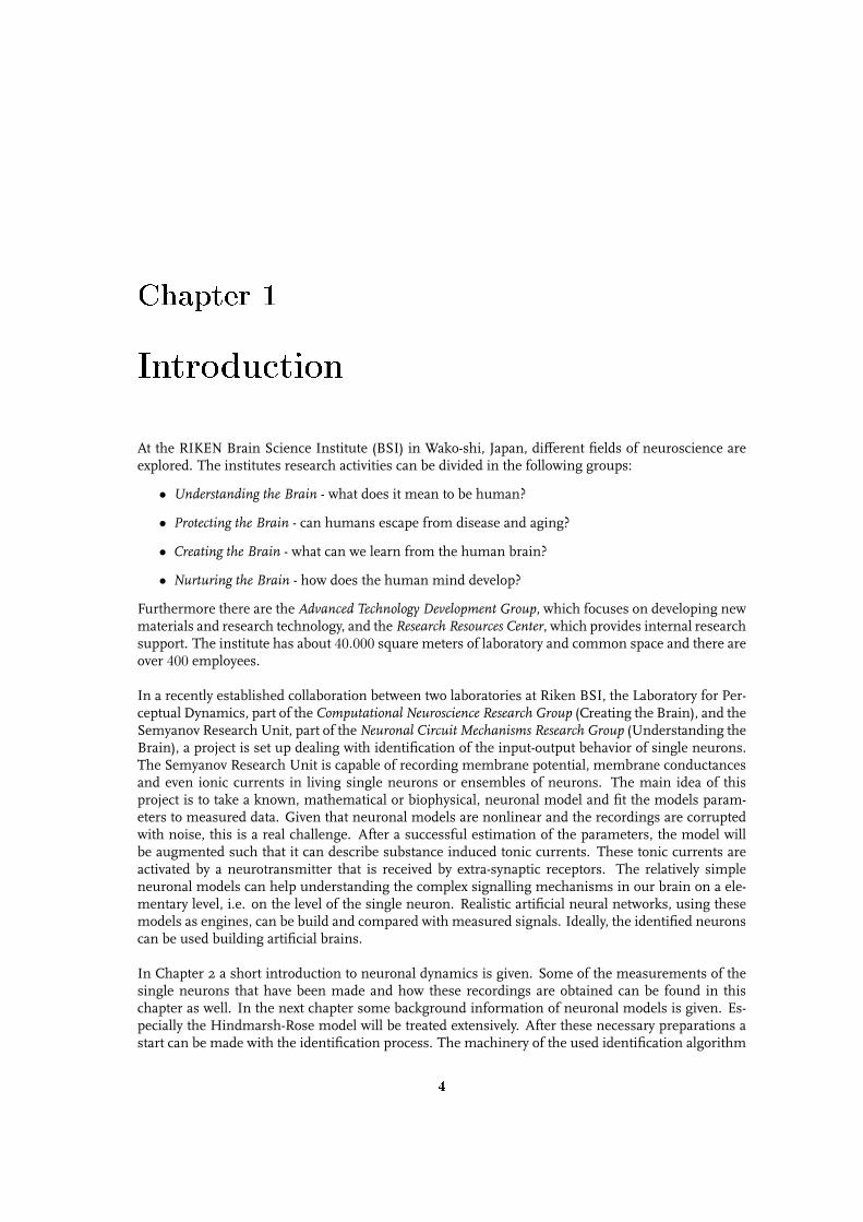
At the RIKEN Brain Science Institute (BSI) in Wako-shi, Japan, different fields of neuroscience areexplored. The institutes research activities can be divided in the following groups:
• Understanding the Brain - what does it mean to be human?
• Protecting the Brain - can humans escape from disease and aging?
• Creating the Brain - what can we learn from the human brain?
• Nurturing the Brain - how does the human mind develop?
Furthermore there are the Advanced Technology Development Group, which focuses on developing newmaterials and research technology, and the Research Resources Center, which provides internal researchsupport. The institute has about 40.000 square meters of laboratory and common space and there areover 400 employees.
In a recently established collaboration between two laboratories at Riken BSI, the Laboratory for Per-ceptual Dynamics, part of the Computational Neuroscience Research Group (Creating the Brain), and theSemyanov Research Unit, part of the Neuronal Circuit Mechanisms Research Group (Understanding theBrain), a project is set up dealing with identification of the input-output behavior of single neurons.The Semyanov Research Unit is capable of recording membrane potential, membrane conductancesand even ionic currents in living single neurons or ensembles of neurons. The main idea of thisproject is to take a known, mathematical or biophysical, neuronal model and fit the models param-eters to measured data. Given that neuronal models are nonlinear and the recordings are corruptedwith noise, this is a real challenge. After a successful estimation of the parameters, the model willbe augmented such that it can describe substance induced tonic currents. These tonic currents areactivated by a neurotransmitter that is received by extra-synaptic receptors. The relatively simpleneuronal models can help understanding the complex signalling mechanisms in our brain on a ele-mentary level, i.e. on the level of the single neuron. Realistic artificial neural networks, using thesemodels as engines, can be build and compared with measured signals. Ideally, the identified neuronscan be used building artificial brains.
In Chapter 2 a short introduction to neuronal dynamics is given. Some of the measurements of thesingle neurons that have been made and how these recordings are obtained can be found in thischapter as well. In the next chapter some background information of neuronal models is given. Es-pecially the Hindmarsh-Rose model will be treated extensively. After these necessary preparations astart can be made with the identification process. The machinery of the used identification algorithm
4

is explained in Chapter 4, followed by some obtained results which are written down in Chapter 5.Chapter 6 completes the report with conclusions and recommendations.
1.1 NotationsThroughout this report the following notations will be used. The symbol R denotes the field of realnumbers. The symbol R+ indicates the positive real numbers. The Euclidian norm in x ∈ Rn
is denoted by ‖x‖. For a vector field f on Rn and a function g on Rm we denote by Lkf g the kth
directional derivative of g with respect to f thus L0fg = g, Lk+1
f g = Lf
(Lk
f g)
. By Ln∞[t0, T ] we
denote the space of all functions f : R+ → Rn such that ‖f‖∞,[t0,T ] = sup‖f(t)‖, t ∈ [t0, T ] < ∞,and ‖f‖∞,[t0,T ] stands for the Ln
∞[t0, T ] norm of f(t). Let A be a set in Rn, and ‖ · ‖ be the usualEuclidean norm in Rn. By ‖·‖A the following induced norm is denoted:
‖x‖A = infq∈A
‖x− q‖.
Finally, the notation ‖x‖A∆stands for the following:
‖x‖A∆=
‖x‖A −∆, ‖x‖A > ∆0, ‖x‖A ≤ ∆
for some ∆ ∈ R+.
5
Chapter 2
Neuronal Dynamics
The brain computes! Sensory signals are transformed into various biophysical variables, such asmembrane potential and firing rates, which are subsequently used in various processes we call com-putations. An important element in this signaling process is the single neuron. In the beginningneurons were regarded as single functional units, which could only act in active or resting state. Inthe last 50 years the view on signalling and the role of single neurons has been changed tremen-dously, realizing now information is encoded in membrane potential and firing rates and signalsdecay in distance [1].
2.1 SignallingA single neuron can be represented as an electrical circuit, build of different compartments consistingof capacitors, conductances and leak voltages. Each neuron has a resting state with correspondingresting potential Vrest, which value can vary from as high as -30mV to as low as -90mV dependingon circumstances. In this state the neuron is in a dynamical equilibrium. Ionic currents, particularysodium and potassium current, are flowing across the membrane in such a way that the net currentis zero. Applying some stimuli will force the neuron from this equilibrium and make the neuronexcitable. If the stimuli is large enough such that a threshold value, the threshold potential Vthres, iscrossed, the neuron will generate action potentials and starts to fire. On the other hand, if the stimuliis such that Vthres is not passed, the neuron will return to its resting state.
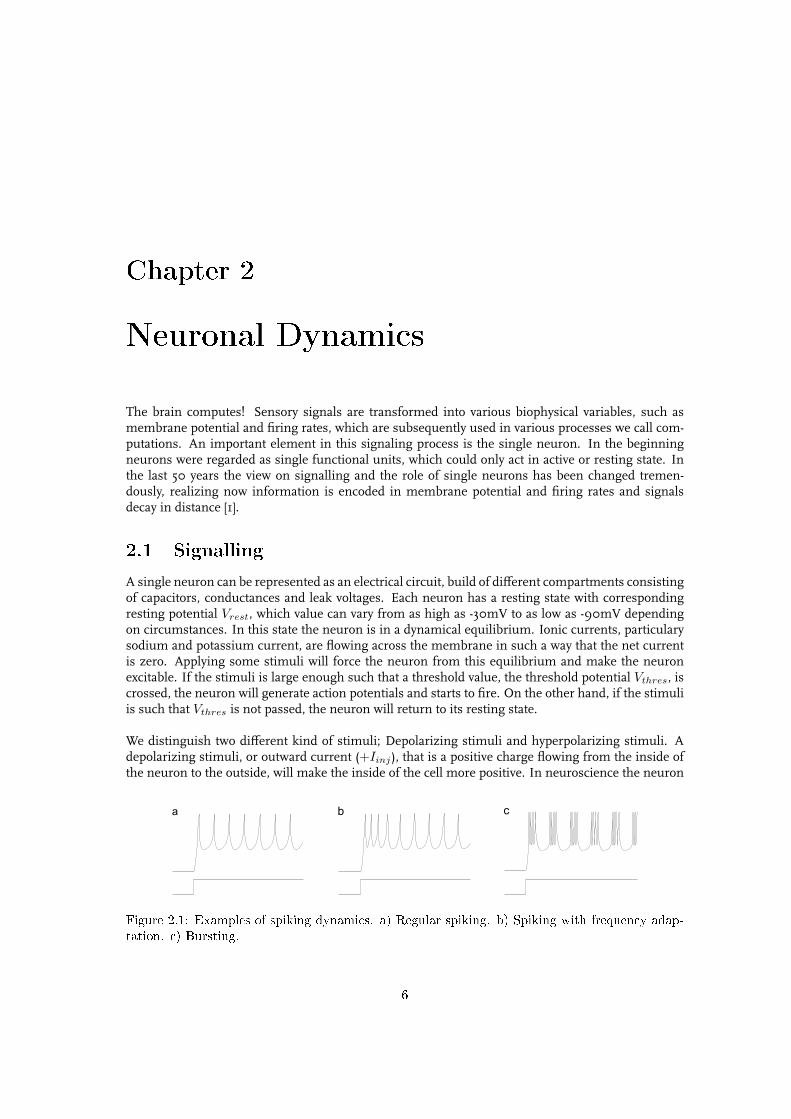
We distinguish two different kind of stimuli; Depolarizing stimuli and hyperpolarizing stimuli. Adepolarizing stimuli, or outward current (+Iinj), that is a positive charge flowing from the inside ofthe neuron to the outside, will make the inside of the cell more positive. In neuroscience the neuron
a b c
Figure 2.1: Examples of spiking dynamics. a) Regular spiking. b) Spiking with frequency adap-tation. c) Bursting.
6
is said to be depolarized. An inward current (−Iinj) will make the inside of the cell more negative, theneuron is called hyperpolarized. The signals generated by the neuron as response on stimuli do existin various modes depending on the type of neuron and stimuli. Figure 2.1 shows some examples ofdifferent modes of spiking dynamics or spike trains. Detailed information about biophysical featuresand different spiking modes can be found in [6].
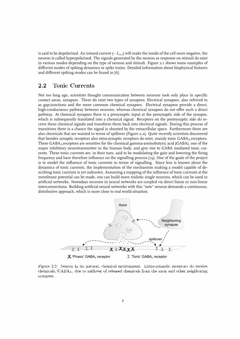
2.2 Tonic CurrentsNot too long ago, scientists thought communication between neurons took only place in specificcontact areas, synapses. There do exist two types of synapses; Electrical synapses, also referred toas gap-junctions and the more common chemical synapses. Electrical synapses provide a direct,high-conductance pathway between neurons, whereas chemical synapses do not offer such a directpathway. At chemical synapses there is a presynaptic input at the presynaptic side of the synapse,which is subsequently translated into a chemical signal. Receptors on the postsynaptic side do re-ceive these chemical signals and transform them back into electrical signals. During this process oftransitions there is a chance the signal is shunted by the extracellular space. Furthermore there arealso chemicals that are waisted in terms of spillover (Figure 2.2). Quite recently scientists discoveredthat besides synaptic receptors also extra-synaptic receptors do exist, mainly tonic GABAAreceptors.These GABAAreceptors are sensitive for the chemical gamma-aminobutyric acid (GABA), one of themajor inhibitory neurotransmitter in the human body, and give rise to GABA mediated tonic cur-rents. These tonic currents are, in their turn, said to be modulating the gain and lowering the firingfrequency and have therefore influence on the signalling process [19]. One of the goals of the projectis to model the influence of tonic currents in terms of signalling. Since less is known about thedynamics of tonic currents, the implementation of the mechanism making a model capable of de-scribing tonic currents is yet unknown. Assuming a mapping of the influence of tonic currents at themembrane potential can be made, one can build more realistic single neurons, which can be used inartificial networks. Nowadays neurons in neural networks are coupled via direct linear or non-linearinterconnections. Building artificial neural networks with this "new" neuron demands a continuous,distributive approach, which is more close to real world situation.
‘Phasic’ GABA receptorA ‘Tonic’ GABA receptorA
spillover
Axon
Neighboringsynapse
Figure 2.2: Neuron in its natural, chemical environment. Extra-synaptic receptors do receivechemicals, GABAA, due to spillover of released chemicals from the axon and other neighboringsynapses.
7
200 mm
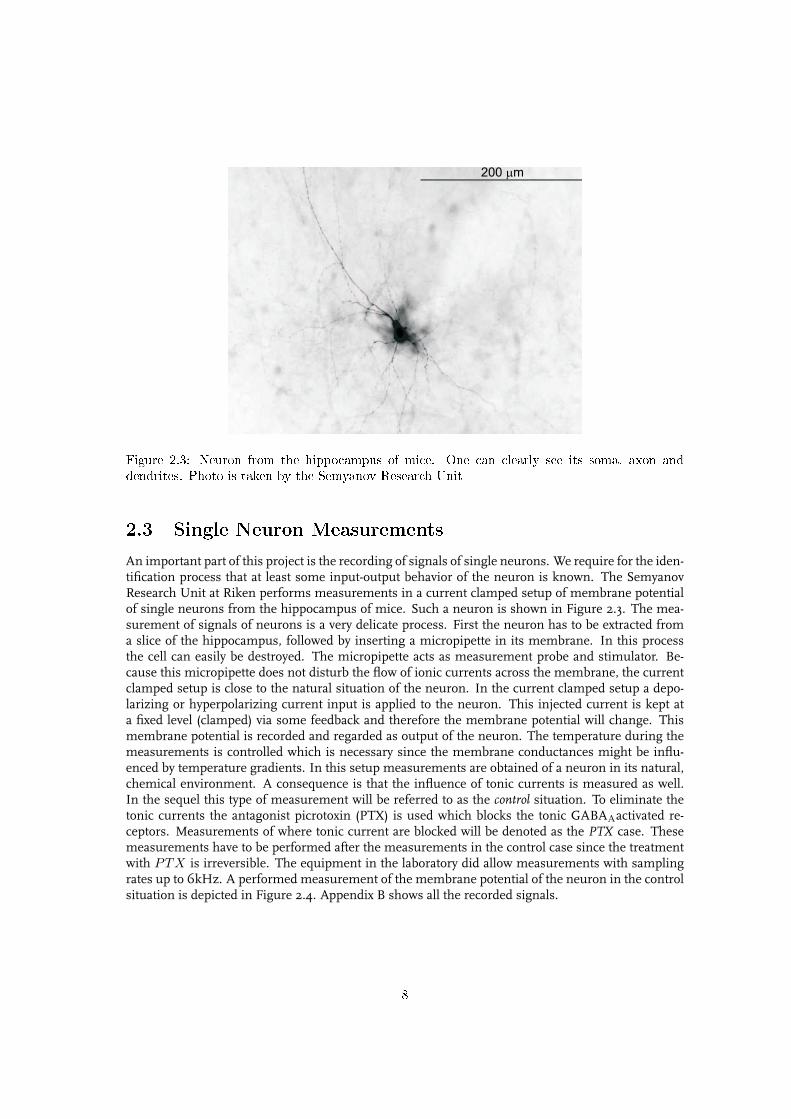
Figure 2.3: Neuron from the hippocampus of mice. One can clearly see its soma, axon anddendrites. Photo is taken by the Semyanov Research Unit
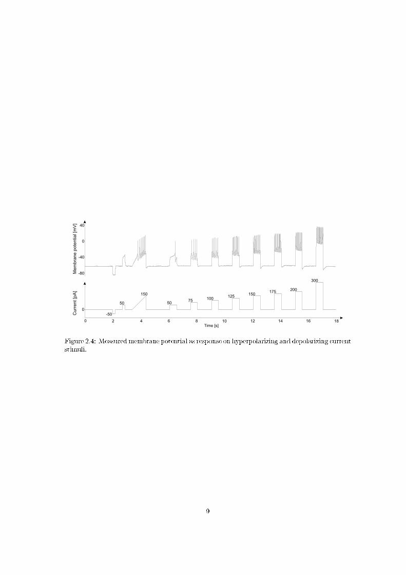
2.3 Single Neuron MeasurementsAn important part of this project is the recording of signals of single neurons. We require for the iden-tification process that at least some input-output behavior of the neuron is known. The SemyanovResearch Unit at Riken performs measurements in a current clamped setup of membrane potentialof single neurons from the hippocampus of mice. Such a neuron is shown in Figure 2.3. The mea-surement of signals of neurons is a very delicate process. First the neuron has to be extracted froma slice of the hippocampus, followed by inserting a micropipette in its membrane. In this processthe cell can easily be destroyed. The micropipette acts as measurement probe and stimulator. Be-cause this micropipette does not disturb the flow of ionic currents across the membrane, the currentclamped setup is close to the natural situation of the neuron. In the current clamped setup a depo-larizing or hyperpolarizing current input is applied to the neuron. This injected current is kept ata fixed level (clamped) via some feedback and therefore the membrane potential will change. Thismembrane potential is recorded and regarded as output of the neuron. The temperature during themeasurements is controlled which is necessary since the membrane conductances might be influ-enced by temperature gradients. In this setup measurements are obtained of a neuron in its natural,chemical environment. A consequence is that the influence of tonic currents is measured as well.In the sequel this type of measurement will be referred to as the control situation. To eliminate thetonic currents the antagonist picrotoxin (PTX) is used which blocks the tonic GABAAactivated re-ceptors. Measurements of where tonic current are blocked will be denoted as the PTX case. Thesemeasurements have to be performed after the measurements in the control case since the treatmentwith PTX is irreversible. The equipment in the laboratory did allow measurements with samplingrates up to 6kHz. A performed measurement of the membrane potential of the neuron in the controlsituation is depicted in Figure 2.4. Appendix B shows all the recorded signals.
8
0 2 4 6 8 10 12 14 16 18
-50
50
150100
5075
125150
175200
300
0
-80
-40
0
40
Me
mb
ran
e p
ote
ntia
l [m
V]
Cu
rre
nt
[pA
]
Time [s]
Figure 2.4: Measured membrane potential as response on hyperpolarizing and depolarizing currentstimuli.
9
Chapter 3
Hindmarsh-Rose Neuronal Model
Throughout the years, many neuronal models are developed for different purposes. These modelsvary from true biophysical ones, like the Hodgkin-Huxley model, to simplified models for studyingsynchronization theories in large ensembles of neurons. Which model to use depends mainly on thebiological features that need to be described and the costs of implementation.
3.1 Neuronal ModelsIn this section a brief overview of different neuronal models will be presented. More detailed infor-mation can be found in [6].
a. Biophysical modelsOne of the most important model in computational neuroscience is the 1952 Hodgkin-Huxley model[5]. Hodgkin and Huxley gave an explanation of action potential generation in the axon of the giantsquid in terms of time- and voltage-dependent sodium and potassium conductances, GNa and GK re-spectively. The state of GNa is governed by three activation particles m and one inactivating particle h.The sodium conductance is regulated by four activating particles n. The dynamics of these particlesis given by first-order differential equations consisting of voltage dependent terms, time constantsand steady-state activation or inactivation, bringing up the total number of differential equations tofour. Morris-Lecar suggested a simple, two-dimensional model to describe oscillations in barnaclegiant muscle fiber. Just like the Hodgkin-Huxley model, the Morris-Lecar model consists of a mem-brane potential equation and two currents. However, this model contains two activation particles nand m, from which only particle n is described using a differential equation. Although this model isable to reproduce various types of spiking, it can not exhibit bursting modes without adding an extraequation. These biological models are beloved by biophysicists since they are biophysically plausibleand the parameters are in most cases measurable. However, they are very expensive in terms of flopsand the number of parameters is large. To obtain a fit of the recorded signals to a biophysical modelit is required to measure all individual ionic currents. Since for this study only input-output signalsare measured it is not possible to use a biophysical model.
b. Integrate-and-Fire modelsThe most simple neuronal model is the so called Integrate-and-Fire model, which is widely usedin computational neuroscience. Perfect Integrate-and-Fire models describe the behavior in a sub-threshold domain where the neuron is modeled using only a single capacitance. When the thresholdis crossed the neuron is said to be firing. Integrate-and-Fire models come in several flavors. One
10
popular variant of the Integrate-and-Fire model is the Leaky-Integrate-and-Fire model,
v = I + a− bv, if v ≥ vth, then v ← c, (3.1)
where v equals the membrane potential, I is the input current, a, b, c are parameters, and vth repre-sents the threshold value. If state v passes vth,the state is resetted to c. Although these models areefficient, they can only feature very little types of spiking behavior. Other variants such as Integrate-and-Fire-or-Burst or Integrate-and-Fire-with-Adaptation are able to produce more of the biologicalfeatures. However, none of the Integrate-and-Fire models do give a realistic description of the spik-ing dynamics of the neuron and therefore they are actually only used to test analytical results orsimulate very large ensembles of neurons.
c. Phase-plane modelsBetween the biophysical models on the one hand and the simple Integrate-and-Fire models on theother hand, there is a third category of models which we will refer as phase-plane models, since itsdynamics can be relatively easy understood throughout phase-plane analysis. These models can ex-hibit a large number of biophysical features and are relatively simple and efficient. These proportiesmake phase-plane models very suitable for the goals of this particular project. The identification willtherefore be based on one of the most complete phase-plane models, the Hindmarsh-Rose model.
3.2 The 1982 ModelThe Hindmarsh-Rose equations are developed to study synchronization of firing of two snail neuronswithout the need to use the full Hodgkin-Huxley equations. The natural choice that time was touse the FitzHugh-Nagumo model, which is more or less a simplification of the Hodgkin-Huxleyequations. FitzHugh and Nagumo observed independently that in the Hodgkin-Huxley equations,the membrane potential V (t) as well as sodium activation m(t) evolve on similar time-scales duringan action potential, while sodium inactivation h(t) and potassium activation n(t) change on similar,although slower time scales. As a result, a model simulating spiking behavior can now be representedby the following equations
x = a(y − f(x) + I(t)),y = b(g(x)− y) , (3.2)
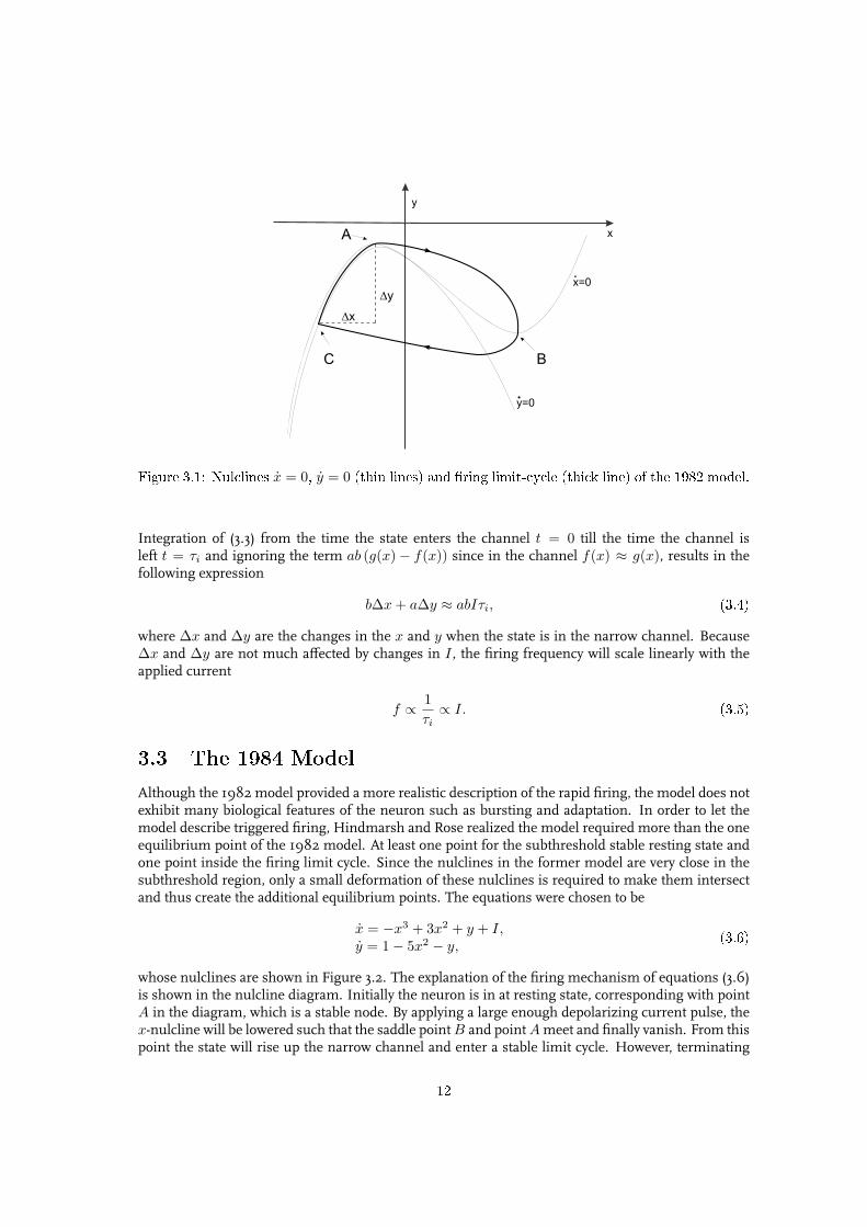
where state x represents membrane potential and y an recovery variable. The function f(x) is cu-bic, the function g(x) is linear, parameters a, b are time constants and I(t) is the external appliedor clamping current as function of time t. However, this model does not provide a very realistic de-scription of the rapid firing of the neuron compared to the relatively long interval between firing. Intheir attempts to achieve a more realistic description of firing, Hindmarsh and Rose did replace thelinear function g(x) in the FitzHugh-Nagumo equations with a quadratic function. How this slightmodification makes the model capable describing rapid firing with a long interspike interval can beexplained looking at the nulcline diagram, shown in Figure 3.1. When the limit-cycle crosses the x-nulcline at C, it is trapped in the narrow channel between the nulclines and can leave only near pointA. In this channel, both x and y are small since the state is close to both nulclines and thereforethe state changes slowly, which gives rise to a large, more realistic interspike interval. Furthermore,this model gives an explanation for the approximately linear relationship between firing frequency fand the applied external current I(t). Let the interspike interval τi be the time spent in the narrowchannel. From a linear combination of the equations (3.2) we obtain
bx + ay = ab (g(x)− f(x)) + abI. (3.3)
11
xA
BC
y=0
x=0
y
Dx
Dy
Figure 3.1: Nulclines x = 0, y = 0 (thin lines) and ring limit-cycle (thick line) of the 1982 model.
Integration of (3.3) from the time the state enters the channel t = 0 till the time the channel isleft t = τi and ignoring the term ab (g(x)− f(x)) since in the channel f(x) ≈ g(x), results in thefollowing expression
b∆x + a∆y ≈ abIτi, (3.4)
where ∆x and ∆y are the changes in the x and y when the state is in the narrow channel. Because∆x and ∆y are not much affected by changes in I , the firing frequency will scale linearly with theapplied current
f ∝ 1τi∝ I. (3.5)
3.3 The 1984 ModelAlthough the 1982 model provided a more realistic description of the rapid firing, the model does notexhibit many biological features of the neuron such as bursting and adaptation. In order to let themodel describe triggered firing, Hindmarsh and Rose realized the model required more than the oneequilibrium point of the 1982 model. At least one point for the subthreshold stable resting state andone point inside the firing limit cycle. Since the nulclines in the former model are very close in thesubthreshold region, only a small deformation of these nulclines is required to make them intersectand thus create the additional equilibrium points. The equations were chosen to be
x = −x3 + 3x2 + y + I,y = 1− 5x2 − y,
(3.6)
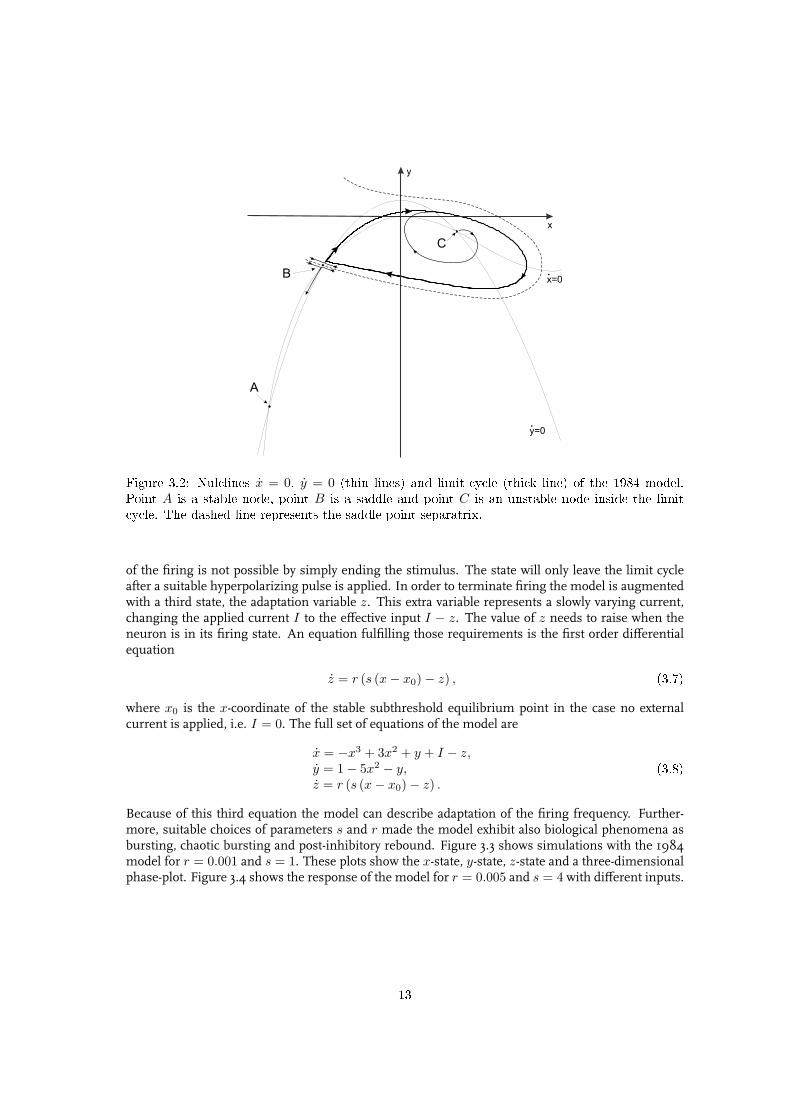
whose nulclines are shown in Figure 3.2. The explanation of the firing mechanism of equations (3.6)is shown in the nulcline diagram. Initially the neuron is in at resting state, corresponding with pointA in the diagram, which is a stable node. By applying a large enough depolarizing current pulse, thex-nulcline will be lowered such that the saddle point B and point A meet and finally vanish. From thispoint the state will rise up the narrow channel and enter a stable limit cycle. However, terminating
12
x
A
B
C
y=0
x=0
y
Figure 3.2: Nulclines x = 0, y = 0 (thin lines) and limit-cycle (thick line) of the 1984 model.Point A is a stable node, point B is a saddle and point C is an unstable node inside the limitcycle. The dashed line represents the saddle point separatrix.
of the firing is not possible by simply ending the stimulus. The state will only leave the limit cycleafter a suitable hyperpolarizing pulse is applied. In order to terminate firing the model is augmentedwith a third state, the adaptation variable z. This extra variable represents a slowly varying current,changing the applied current I to the effective input I − z. The value of z needs to raise when theneuron is in its firing state. An equation fulfilling those requirements is the first order differentialequation
z = r (s (x− x0)− z) , (3.7)
where x0 is the x-coordinate of the stable subthreshold equilibrium point in the case no externalcurrent is applied, i.e. I = 0. The full set of equations of the model are
x = −x3 + 3x2 + y + I − z,y = 1− 5x2 − y,z = r (s (x− x0)− z) .
(3.8)
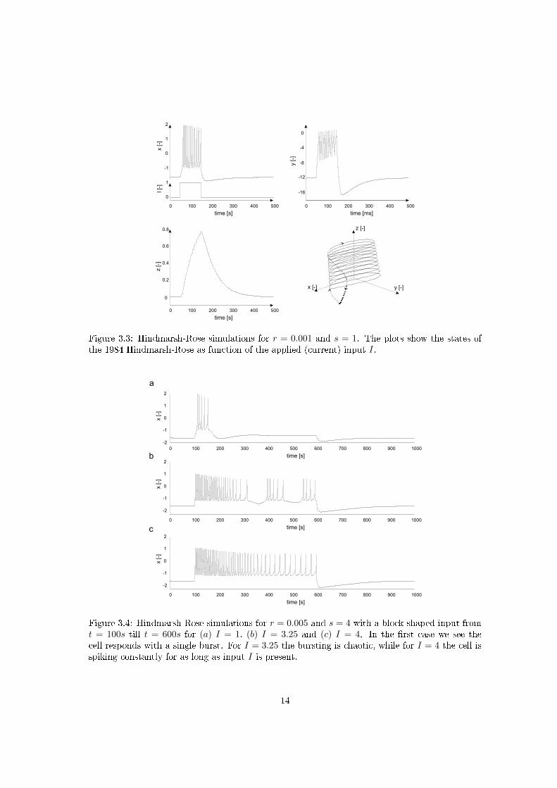
Because of this third equation the model can describe adaptation of the firing frequency. Further-more, suitable choices of parameters s and r made the model exhibit also biological phenomena asbursting, chaotic bursting and post-inhibitory rebound. Figure 3.3 shows simulations with the 1984model for r = 0.001 and s = 1. These plots show the x-state, y-state, z-state and a three-dimensionalphase-plot. Figure 3.4 shows the response of the model for r = 0.005 and s = 4 with different inputs.
13
0 100 200 300 400 500
0
1
-1
0
1
2
time [s]
x [-]
-16
-12
-8
-4
0
y [-]
0
0.2
0.4
0.6
0.8
z [-]
x [-] y [-]
z [-]
I [-
]
0 100 200 300 400 500
time [ms]
0 100 200 300 400 500
time [s]
Figure 3.3: Hindmarsh-Rose simulations for r = 0.001 and s = 1. The plots show the states ofthe 1984 Hindmarsh-Rose as function of the applied (current) input I.
0 100 200 300 400 500 600 700 800 900 1000
-2
-1
0
1
2
x [-]
0 100 200 300 400 500 600 700 800 900 1000
-2
-1
0
1
2
time [s]
time [s]
x [-]
0 100 200 300 400 500 600 700 800 900 1000
-2
-1
0
1
2
time [s]
x [-]
a
b
c
Figure 3.4: Hindmarsh-Rose simulations for r = 0.005 and s = 4 with a block-shaped input fromt = 100s till t = 600s for (a) I = 1, (b) I = 3.25 and (c) I = 4. In the rst case we see thecell responds with a single burst. For I = 3.25 the bursting is chaotic, while for I = 4 the cell isspiking constantly for as long as input I is present.
14

15

Chapter 4
Identication: Parameter and StateObservations
In this chapter the focus will be on the (off-line) technique to estimate the parameters of the Hindmarsh-Rose model from the measured input-output data. It will be assumed the membrane potential can becompletely described by the Hindmarsh-Rose equations
S =
x1 = 1Ts
(−ax31 + bx2
1 + x2 − x3 + a0u(t)),
x2 = 1Ts
(c− dx2
1 − βx2
),
x3 = 1Ts
r (s (x1 − x0)− x3) ,(4.1)
where x = [x1 x2 x3]T ∈ R3, input u(t) ∈ R and constants a, a0, b, c, d, β, r, s, x0 > 0. The statex1 represents membrane potential, x2 is an internal fast current and x3 represents a slow varyingcurrent. The constant Ts is a time scaling factor that allows the output of the Hindmarsh-Rose modelto be in the millisecond time range instead of seconds. However, instead of using this time scalingfactor it is also possible to "stretch" the time axis of the measured signals. In this study the timeaxis of the measured signal will be multiplied with a factor 1000 and therefore Ts = 1 will be used.Signals x1(t), u(t) and constant x0 are measurable and therefore assumed to be known. Note thisparametrization of system S is identical to the original 1984 Hindmarsh-Rose equations except forthe constants a0 and a1, which are additional weight factors that provide some extra freedom to obtaina proper fit.
4.1 Adaptive ObserversThe classical way of solving problems where states need to be reconstructed and a number of param-eters need to be estimated is using adaptive observers [8],[14],[15]. Adaptive observer can be designedfor systems of the form:
z = Az + ψ0(y, u) +p∑
i=1
ψi(y, u)θi(t)
y = Cz,(4.2)
16
where z ∈ Rn, y ∈ R, (θ1, · · · , θp) are unknown, possible time-varying parameters and
A =
0 0 · · · 0 01 0 · · · 0 0...
.... . .
......
0 0 · · · 1 0
, C =
[0 0 · · · 0 1
].
The system (4.2) is said to be in adaptive observer canonical form. However, the Hindmarsh-Roseequations are given, like most non-linear systems, in the following form:
x = f(x) + q0(x, u) +p∑
i=1
θiqi(x, u)
= f(x) + q0(x, u) + Q(x, u)θ,
y = h(x),
(4.3)
where x ∈ Rn, u ∈ Rm, θ ∈ Rp, y ∈ R and smooth functions f : Rn → Rn, h : Rn → R andqi : Rn ×Rm → Rn, 0 ≤ i ≤ p. The parameter vector θ is supposed to be constant, x is the state andu(t) is the (control) input which is known. System (4.3) has to be transformed into system (4.2) viaa coordinate transformation z = Φ(x). A necessary condition for the existence of such a coordinatetransformation is that (f , h) is an observable pair, i.e. the following should hold:
rank
d(Lj
fh(x))
: 0 ≤ j ≤ n− 1
= n, ∀x ∈ Rn. (4.4)
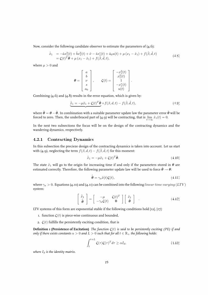
In the case of system S this condition is not fulfilled. Therefore it is not possible to use adaptiveobservers for the estimation of the states and parameters for the system.
4.2 Attracting and Wandering DynamicsSince it is not possible to transform system S into the adaptive observer canonical form, and thusit is not possible to make use of an adaptive observer, a technique using contracting and wanderingdynamics will be proposed to estimate the parameters of the Hindmarsh-Rose model. Thereforethe system dynamics will be decomposed into two interconnected subsystems. The first subsystemconsists of a stable, contracting part while the dynamics of the second subsystem are wandering.Detailed information about contracting and wandering dynamics can be found in [21], from which apreprint version is included in Appendix D.
First some feedback will be designed such the the error equation, that is the equation that describesthe error between signal x1 and the estimated signal x1, is of the following form:
˙x1 = f0(x1, t) + f(ξ(t), θw)− f(ξ(t), θw), (4.5)
where x1 = x1 − x1, x1 ∈ R, θw, θw ∈ Ωθw ⊂ R2, functions ξ : R+ → R, f0 : R → R, f :R × R2 → R. The function ξ(t) is a function of time which includes available measurements ofthe state. The vectors θw, θw contain the unknown and estimated parameters respectively whichbelong to a bounded set Ωθw . The function f0(·) represents the contracting dynamics and the partf(ξ(t), θw)− f(ξ(t), θw) represents the wandering dynamics.
In order to estimate the Hindmarsh-Rose parameters using contracting and wandering dynamics,the three-dimensional system S will be rewritten into the one-dimensional system:
x1 = −ax31 + bx2
1 + ν + f(β, d, t)− sx∗1 + a0u(t), (4.6)
17
where
ν =c
β, f(β, d, t) = e−β(t−t0)x2(t0) +
t∫
0
e−β(t−τ)dx21(τ)dτ.
The expression ν + f(β, d, t) is the analytical solution of the x2-dynamics of S . In the sequel theexponential decaying part of f(β, d, t) will be neglected such that
f(β, d, t) =
t∫
0
e−β(t−τ)dx21(τ)dτ.
The x3-dynamics of the Hindmarsh-Rose equations can be considered as a low-pass filter. The signalx3 can be written as filter-gain s multiplied by the filtered signal (x1 − x0) using filter
H(jω) =1
1r jω + 1
. (4.7)
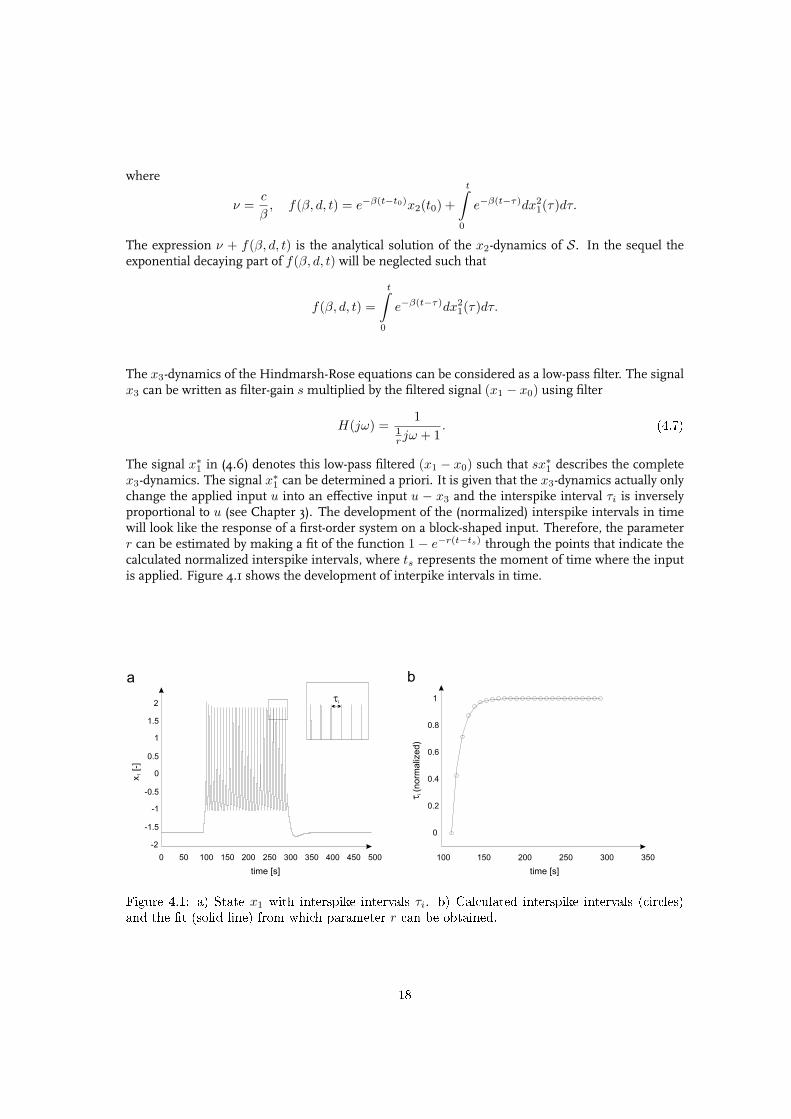
The signal x∗1 in (4.6) denotes this low-pass filtered (x1 − x0) such that sx∗1 describes the completex3-dynamics. The signal x∗1 can be determined a priori. It is given that the x3-dynamics actually onlychange the applied input u into an effective input u − x3 and the interspike interval τi is inverselyproportional to u (see Chapter 3). The development of the (normalized) interspike intervals in timewill look like the response of a first-order system on a block-shaped input. Therefore, the parameterr can be estimated by making a fit of the function 1 − e−r(t−ts) through the points that indicate thecalculated normalized interspike intervals, where ts represents the moment of time where the inputis applied. Figure 4.1 shows the development of interpike intervals in time.
0 50 100 150 200 250 300 350 400 450 500
-2
-1.5
-1
-0.5
0
0.5
1
1.5
2
100 150 200 250 300 350
0
0.2
0.4
0.6
0.8
1
time [s]
ti(n
orm
aliz
ed
)
time [s]
x[-
]1
ti
a b
Figure 4.1: a) State x1 with interspike intervals τi. b) Calculated interspike intervals (circles)and the t (solid line) from which parameter r can be obtained.
18
Now, consider the following candidate observer to estimate the parameters of (4.6):
˙x1 = −ax31(t) + bx2
1(t) + ν − sx∗1(t) + a0u(t) + µ (x1 − x1) + f(β, d, t)= ζ(t)T θ + µ (x1 − x1) + f(β, d, t),
(4.8)
where µ > 0 and
θ =
abνsa0
, ζ(t) =
−x31(t)
x21(t)1
−x∗1(t)u(t)
.
Combining (4.6) and (4.8) results in the error equation, which is given by:
˙x1 = −µx1 + ζ(t)T θ︸ ︷︷ ︸+f(β, d, t)− f(β, d, t), (4.9)
where θ = θ− θ. In combination with a suitable parameter update law the parameter error θ will beforced to zero. Then, the underbraced part of (4.9) will be contracting, that is lim
t→∞x1(t) = 0.
In the next two subsections the focus will be on the design of the contracting dynamics and thewandering dynamics, respectively.
4.2.1 Contracting DynamicsIn this subsection the precieze design of the contracting dynamics is taken into account. Let us startwith (4.9), neglecting the term f(β, d, t)− f(β, d, t) for this moment:
˙x1 = −µx1 + ζ(t)T θ. (4.10)
The state x1 will go to the origin for increasing time if and only if the parameters stored in θ areestimated correctly. Therefore, the following parameter update law will be used to force θ → θ:
˙θ = γax(t)ζ(t), (4.11)
where γa > 0. Equations (4.10) and (4.11) can be combined into the following linear time varying (LTV )system:
[˙x1
˙θ
]=
[ −µ ζ(t)T
−γaζ(t) 0
] [x1
θ
]. (4.12)
LTV systems of this form are exponential stable if the following conditions hold [12], [17]:
1. function ζ(t) is piece-wise continuous and bounded,
2. ζ(t) fulfills the persistently exciting condition, that is
Definition 1 (Persistence of Excitation) The function ζ(t) is said to be persistently exciting (PE) if andonly if there exists constants α > 0 and L > 0 such that for all t ∈ R+ the following holds:
∫ t+L
t
ζ(τ)ζ(τ)T dτ ≥ αId, (4.13)
where Id is the identity matrix.
19
Since all signals in ζ(t) are known and indeed piecewise continuous and bounded, condition 1 isfulfilled. Condition 2 has to be investigated (numerically) for each individual case. Assuming bothconditions do hold, system (4.12) is exponentially stable. The rate of convergence ρ is defined as:
‖ w(τ) ‖∞,[t0,t]≤ e−ρ(t−t0) ‖ w0 ‖, (4.14)
where
w =[
x1
θ
], w0 = w(t = t0).
In the sequel it will be assumed, for simplicity, that the convergence rate of the error x1 is equal tothis convergence rate ρ. A rate of convergence larger than ρ does not make the identification methodnot going to work. It only indicates that the gain γw, which will be specified in the next section, canbe increased.
4.2.2 Wandering DynamicsIn this subsection the focus will be on the design of the wandering dynamics. Reconsider the errorequation (4.9) given that the contracting dynamics (4.12) are exponentially stable:
x1 = −ρx1 + f(β, d, t)− f(β, d, t). (4.15)
The wandering dynamics will search for the values of the remaining parameters in some boundeddomain Ωβ × Ωd, where β, β ∈ Ωβ and d, d ∈ Ωd, until f(β, d, t) → f(β, d, t) and thus x1 → 0. Thissearch is performed with low speed, such that the contracting dynamics have time to reach its steadystate.
The first thing that is required is boundedness of the function f(·) in terms of its parameters:
|f(β, d, t)− f(β, d, t)| ≤ |f(β, d, t)− f(β, d, t)|+ |f(β, d, t)− f(β, d, t)|≤ Df,β |β − β|+ Df,d|d− d|,
(4.16)
where
Df,β = maxβ,β∈Ωβ ,d∈Ωd
1
ββd ‖ x2
1(τ) ‖∞,[t0,t]
, Df,d = max
β∈Ωβ
1
β‖ x2
1(τ) ‖∞,[t0,t]
. (4.17)
The derivation of Df,β and Df,d can be found in Appendix A.
Next, the following auxiliary system will be introduced:
λ = Σ(λ), (4.18)
where λ ∈ Ωλ ⊂ Rλ is bounded and Σ : Rλ → Rλ is locally Lipschitz. System (4.18) is assumed tobe Poisson stable in Ωλ, that is:
Definition 2 (Poisson stability) The system (4.18) is called Poisson stable in Ωλ if
∀λ′ ∈ Ωλ, t′ ∈ R+ ⇒ ∃t′′ > t′ :‖ λ(t′′, λ′)− λ′ ‖≤ ε, (4.19)
where ε is an arbitrary small positive constant. Moreover, the trajectory λ(t,λ0) is dense in Ωλ:
∀λ′ ∈ Ωλ, ε ∈ R+ ⇒ ∃t ∈ R+ :‖ λ′ − λ(t, λ0) ‖< ε, (4.20)
where λ0 = λ(t0).
20

Define the system (4.18) with the following set of equations:
λ1 = λ2,
λ2 = −ω21λ1,
λ3 = λ4,
λ4 = −ω22λ3, λ0 = (1, 0, 1, 0)T ,
(4.21)
where ω1, ω2 ∈ R+. Furthermore the Poisson stability criterium is satisfied.
In addition, an output function η(λ) : R4 → R2 is selected that will translate λ into estimations ofthe parameter β and d. This output function is required to be locally Lipschitz, that is:
‖ η(λ′)− η(λ′′) ‖≤ Dη ‖ λ′ − λ′′ ‖, λ′, λ′′ ∈ Ωλ, (4.22)
such that η(Ωλ) is dense in Ωβ×Ωd. For Ωβ = [βmin, . . . , βmax] and Ωd = [dmin, . . . , dmax] functionη(λ) = (η1(λ), η2(λ)) is defined as:
β = η1(λ) = βmax−βmin
2
(2 arcsin(λ1)
π + 1)
+ βmin,
d = η2(λ) = dmax−dmin
2
(2 arcsin(λ3)
π + 1)
+ dmin.(4.23)
The Lipschitz constant Dη in (4.22) for the chosen η(λ) is given by:
Dη = max(
(βmax − βmin) · ω1
π,(dmax − dmin) · ω2
π
). (4.24)
The constants ω1 and ω2 in (4.21) need to be chosen with some care. Only by choosing ω1ω2
equal toan irrational number, we ensure that every point in the domain Ωβ × Ωd is visited. More details aregiven in Figure 4.2.
b
d d
d drationalw
1
w2
=
irrationalw
1
w2
=
Dt Dt
Dt Dt
b
b b
d
b
d
b
Figure 4.2: The gure on top shows the case that ω1ω2
is a rational number. As a result, the searchwill nally end up at the same points, even if time goes to innity. In the case where ω1
ω2is an
irrational number, every point in the searching domain Ωβ × Ωd is visited after sucient time.
21
Finally, an accurate interconnection between the contracting dynamics and the wandering dynamicsneeds to be determined. This interconnection will be defined as follows:
λ1 = γw ‖ x1(t) ‖∆(δ) ·λ2,
λ2 = −γw ‖ x1(t) ‖∆(δ) ·ω21λ1,
λ3 = γw ‖ x1(t) ‖∆(δ) ·λ4,
λ4 = −γw ‖ x1(t) ‖∆(δ) ·ω22λ3, λ0 = (1, 0, 1, 0)T ,
(4.25)
where δ > 0 is a pre-defined error tolerance. Furthermore the gain γw satisfies the inequality:
0 < γw ≤ −ρ
(ln
ds
κDβ
)−1κ− 1
κ
1
Dλ
(Dβ
(1 + κ
1−ds
)+ 1
) , (4.26)
with Dβ = 1, Dλ = max(Df,β , Df,d) ·Dη · maxλ∈Ωλ
‖ Σ(λ) ‖, ds ∈ (0, 1) and κ ∈ (1,∞).
By choosing the gain γw according to (4.26), we ensure the contracting part has enough time to reachits steady-state. More detail about the derivation of (4.26) can be found in the section D.5 of the Ap-pendix. Now, for some θ′ in a neighborhood of θ, β′ in a neighborhood of β and d′ in a neighborhoodof d, in combination with the observer (4.8), wandering dynamics (4.23) and interconnection (4.25),the following does hold:
limt→∞
‖ x1 ‖= 0, limt→∞
θ = θ′, limt→∞
β(t) = β′, limt→∞
d(t) = d′,
which should result in a successful fit of the measurements to the model.
The identification algorithm is implemented in Matlab, which code can be found in Appendix C.This implementation in Matlab is rather slow, probably due to the large number of function calls inthe ode-solver. A solution to this problem is found in implementing the algorithm in the low-levelprogramming langue C++, which turns out to be more then hundred times faster then the Matlabalgorithm with similar accuracy. This implementation can be found in Appendix C as well. Notethat this C++ algorithm is not at its final stage. For instance, it is not possible with the presentedalgorithm to keep track of the error, something that is strongly recommended in problems like this.
4.3 Searching Domain Ωβ × Ωd
For the wandering dynamics it is required that the searching domain Ωβ × Ωd is known. Of courseit is always possible to choose some arbitrary domain. However, there is a chance that an arbitrarychosen searching domain will not include the "real" parameter values. On the other hand, the domaincan be chosen too large such that it will take a long time to find the right parameter values. Thereforethe searching domain will be estimated using a feasibility study based on stability proporties of theHindmarsh-Rose model.
It is known that the 1984 model has three equilibrium points, which will be denoted by x0, xth, xsp
representing the stable resting potential, the threshold value and the equilibrium point inside thelimit cycle, respectively. These equilibrium points are given by the roots of the equation:
x31 + px2
1 = q, (4.27)
where
p =1a
(d
β− b
), q =
1a
(a0u(t) +
c
β
)
22
x
x +px3 2
4p27
3
-2p3
q
x0 xth xsp
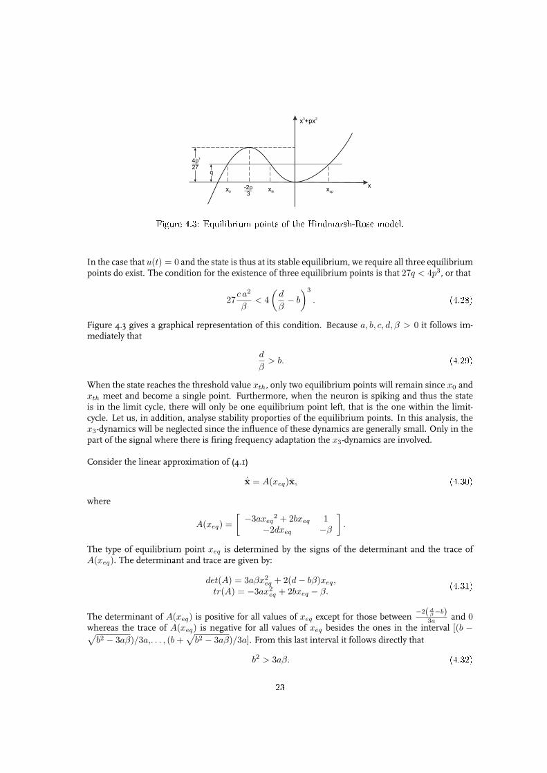
Figure 4.3: Equilibrium points of the Hindmarsh-Rose model.
In the case that u(t) = 0 and the state is thus at its stable equilibrium, we require all three equilibriumpoints do exist. The condition for the existence of three equilibrium points is that 27q < 4p3, or that
27c a2
β< 4
(d
β− b
)3
. (4.28)
Figure 4.3 gives a graphical representation of this condition. Because a, b, c, d, β > 0 it follows im-mediately that
d
β> b. (4.29)
When the state reaches the threshold value xth, only two equilibrium points will remain since x0 andxth meet and become a single point. Furthermore, when the neuron is spiking and thus the stateis in the limit cycle, there will only be one equilibrium point left, that is the one within the limit-cycle. Let us, in addition, analyse stability proporties of the equilibrium points. In this analysis, thex3-dynamics will be neglected since the influence of these dynamics are generally small. Only in thepart of the signal where there is firing frequency adaptation the x3-dynamics are involved.
Consider the linear approximation of (4.1)
˙x = A(xeq)x, (4.30)
where
A(xeq) =[ −3axeq
2 + 2bxeq 1−2dxeq −β
].
The type of equilibrium point xeq is determined by the signs of the determinant and the trace ofA(xeq). The determinant and trace are given by:
det(A) = 3aβx2eq + 2(d− bβ)xeq,
tr(A) = −3ax2eq + 2bxeq − β.
(4.31)
The determinant of A(xeq) is positive for all values of xeq except for those between−2( d
β−b)3a and 0
whereas the trace of A(xeq) is negative for all values of xeq besides the ones in the interval [(b −√b2 − 3aβ)/3a,. . . , (b +
√b2 − 3aβ)/3a]. From this last interval it follows directly that
b2 > 3aβ. (4.32)
23
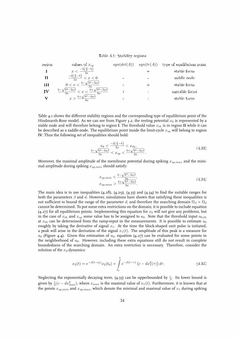
Table 4.1: Stability regions
region values of xeq sgn(det(A)) sgn(tr(A)) type of equilibrium pointI x <
−2( dβ−b)3a - + stable focus
II −2( dβ−b)3a < x < 0 - - saddle node
III 0 < x <b−√
b2−3aβ
3a - + stable focusIV b−
√b2−3aβ
3a < x <b+√
b2−3aβ
3a + + unstable focusV x >
b+√
b2−3aβ
3a - + stable focus
Table 4.1 shows the different stability regions and the corresponding type of equilibrium point of theHindmarsh-Rose model. As we can see from Figure 3.2, the resting potential x0 is represented by astable node and will therefore belong to region I. The threshold value xth is in region II while it canbe described as a saddle-node. The equilibrium point inside the limit-cycle xsp will belong to regionIV. Thus the following set of inequalities should hold:
x0 <−2( d
β−b)3a < xth,
b−√
b2−3aβ
3a < xsp <b+√
b2−3aβ
3a .(4.33)
Moreover, the maximal amplitude of the membrane potential during spiking xsp,max and the mini-mal amplitude during spiking xsp,min should satisfy:
xsp,min <b−√
b2−3aβ
3a ,
xsp,max >b+√
b2−3aβ
3a .(4.34)
The main idea is to use inequalities (4.28), (4.29), (4.33) and (4.34) to find the suitable ranges forboth the parameters β and d. However, simulations have shown that satisfying these inequalities isnot sufficient to bound the range of the parameter d, and therefore the searching domain Ωβ × Ωd
cannot be determined. To put some extra restrictions on the domain, it is possible to include equation(4.27) for all equilibrium points. Implementing this equation for x0 will not give any problems, butin the case of xth and xsp some value has to be assigned to a0. Note that the threshold input a0,th
at xth can be determined from the ramp-input in the measurements. It is possible to estimate a0
roughly by taking the derivative of signal x1. At the time the block-shaped unit pulse is initiated,a peak will arise in the derivation of the signal x1(t). The amplitude of this peak is a measure fora0 (Figure 4.4). Given this estimation of a0, equation (4.27) can be evaluated for some points inthe neighborhood of a0. However, including these extra equations still do not result in completeboundedness of the searching domain. An extra restriction is necessary. Therefore, consider thesolution of the x2-dynamics:
x2(t) = e−β(t−t0)x2(t0) +
t∫
t0
e−β(t−τ)(c− dx2
1(τ))dτ. (4.35)
Neglecting the exponentially decaying term, (4.35) can be upperbounded by cβ . Its lower bound is
given by 1β (c − dx2
max), where xmax is the maximal value of x1(t). Furthermore, it is known that atthe points xsp,min and xsp,max, which denote the minimal and maximal value of x1 during spiking
24
0 10 20 30 40 50 60 70 80 90 100
-2
-1
0
1
2
x[-
]1
-6
-4
-2
0
2
time [s]
dx
/dt
[-]
1
0 10 20 30 40 50 60 70 80 90 100-6
-4
-2
0
2
4
time [s]
dx
/dt
[-]
1
0
1
2
a b
-2
-1
0
1
2
x[-
]1
0
1
2
0 10 20 30 40 50 60 70 80 90 100
time [s]
0 10 20 30 40 50 60 70 80 90 100
time [s]
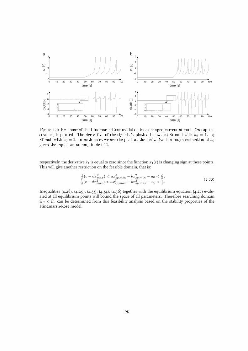
Figure 4.4: Response of the Hindmarsh-Rose model on block-shaped current stimuli. On top thestate x1 is plotted. The derivative of the signals is plotted below. a) Stimuli with a0 = 1. b)Stimuli with a0 = 2. In both cases we see the peak at the derivative is a rough estimation of a0
given the input has an amplitude of 1.
respectively, the derivative x1 is equal to zero since the function x1(t) is changing sign at these points.This will give another restriction on the feasible domain, that is:
1β (c− dx2
max) < ax3sp,min − bx2
sp,min − a0 < cβ ,
1β (c− dx2
max) < ax3sp,max − bx2
sp,max − a0 < cβ .
(4.36)
Inequalities (4.28), (4.29), (4.33), (4.34), (4.36) together with the equilibrium equation (4.27) evalu-ated at all equilibrium points will bound the space of all parameters. Therefore searching domainΩβ × Ωd can be determined from this feasibility analysis based on the stability proporties of theHindmarsh-Rose model.
25

Chapter 5
Main Results
In the previous chapter the technique to make a fit of measured signals to the Hindmarsh-Rosemodel is presented. To properly validate this technique, a signal is generated using the Hindmarsh-Rose equations (4.1). Testing with a generated signal will exclude the possibility that the signal couldnot be described by the model. Furthermore all parameter values are surely constant and known apriori.
5.1 SimulationsThe signal to test the presented identification technique with will be generated from system (4.1) withthe following set of parameters:
a = 1, b = 4, a0 = 1, c = 1, d = 6, β = 1, r = 0.01, s = 1.
As input signal u(t) two 500s long block-shaped current stimuli with amplitudes 0.75 [−] and 1 [−]are applied. The signal has a period of 2000s and is repeated constantly during the parameter estima-tion process. Figure 5.1 shows the input and generated signal.
0 200 400 600 800 1000 1200 1400 1600 1800 2000
0
0.5
1
time [s]
u [-]
-2
-1
0
1
2
3
x1
[-]
0 200 400 600 800 1000 1200 1400 1600 1800 2000
time [s]
Figure 5.1: Simulation generated signal. The gure on the top shows the output x1(t) of thesystem. At the bottom the applied stimuli u(t) is plotted.
26
0 2 4 6 8 10 12 14 16 18 20-1.5
-1
-0.5
0
0.5
1
1.5
time [s]w
[-]
P(t)
w w
x 103
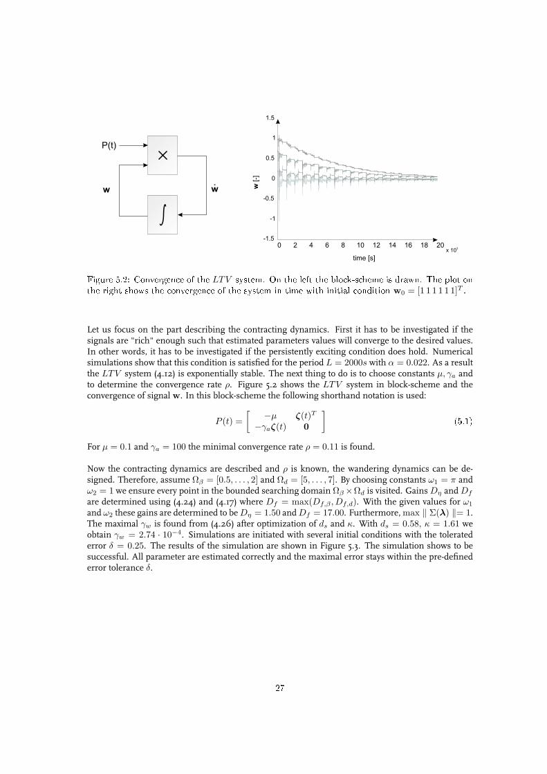
Figure 5.2: Convergence of the LTV system. On the left the block-scheme is drawn. The plot onthe right shows the convergence of the system in time with initial condition w0 = [1 1 1 1 1 1]T .
Let us focus on the part describing the contracting dynamics. First it has to be investigated if thesignals are "rich" enough such that estimated parameters values will converge to the desired values.In other words, it has to be investigated if the persistently exciting condition does hold. Numericalsimulations show that this condition is satisfied for the period L = 2000s with α = 0.022. As a resultthe LTV system (4.12) is exponentially stable. The next thing to do is to choose constants µ, γa andto determine the convergence rate ρ. Figure 5.2 shows the LTV system in block-scheme and theconvergence of signal w. In this block-scheme the following shorthand notation is used:
P (t) =[ −µ ζ(t)T
−γaζ(t) 0
](5.1)
For µ = 0.1 and γa = 100 the minimal convergence rate ρ = 0.11 is found.
Now the contracting dynamics are described and ρ is known, the wandering dynamics can be de-signed. Therefore, assume Ωβ = [0.5, . . . , 2] and Ωd = [5, . . . , 7]. By choosing constants ω1 = π andω2 = 1 we ensure every point in the bounded searching domain Ωβ×Ωd is visited. Gains Dη and Df
are determined using (4.24) and (4.17) where Df = max(Df,β , Df,d). With the given values for ω1
and ω2 these gains are determined to be Dη = 1.50 and Df = 17.00. Furthermore, max ‖ Σ(λ) ‖= 1.The maximal γw is found from (4.26) after optimization of ds and κ. With ds = 0.58, κ = 1.61 weobtain γw = 2.74 · 10−4. Simulations are initiated with several initial conditions with the toleratederror δ = 0.25. The results of the simulation are shown in Figure 5.3. The simulation shows to besuccessful. All parameter are estimated correctly and the maximal error stays within the pre-definederror tolerance δ.
27

0 200 400 600 800 1000 1200 1400 1600 1800 2000-4
-3
-2
-1
0
1
2
3
4
time [s]
x[-
]1
3.9429 3.9429 3.9429 3.9429 3.9429x 10
7
0
1
2
3
4
5
6
7
time [s]
para
mete
r valu
es
[-]
-2
-1.5
-1
-0.5
0
0.5
1
1.5
2
2.5
3
signal
fit
0 200 400 600 800 1000 1200 1400 1600 1800 2000
time [s]
signal
fit
x[-
]1
0 200 400 600 800 1000 1200 1400 1600 1800 2000
-0.1
-0.05
0
0.05
0.1
0.15
0.2
0.25
time [s]
x[-
]1
~
ab
?
s
a0
?
d
0.98
1.00
1.02
Figure 5.3: Simulation results for the test case. On the top-left the t with initial conditions isshown. The plot in the top-right shows the parameters after convergence. In the bottom-left wesee the successful t after parameter convergence and the gure in the bottom-right shows theerror between the signal and the t.
5.2 MeasurementsNow the identification algorithm is successfully validated, the identification using the measured sig-nals can be started. Therefore a single spike train will be selected from the sequence of measure-ments. Only a single spike train is selected to minimize the influence of possible time-varying mem-brane conductances. The criteria for this selection is that the interspike intervals show first orderbehavior. Figure 5.4 shows a selected spike spike train with corresponding interspike intervals. Thisspike train belongs to the first series of measurements in the PTX case, which can be found in Ap-pendix B.
The selected signal will be discarded from noise by filtering it with a Bessel filter, that is a linearlow-pass filter that uses Bessel polynomials. Furthermore the signal will be (spline) interpolated toobtain more measurement points such that smaller time steps can be used in the solver, which inturn should improve accuracy. The measured signal needs to be scaled such that x1(t) is withinthe range [−3, 3] which is a typical output range of the Hindmarsh-Rose model. The signal x1(t)can be obtained by dividing the measured membrane potential Vm(t) by an arbitrary constant. The
28
-100
-50
0
50
mem
bra
ne p
ote
ntial [m
V]
0.5
1
(norm
aliz
ed
)t
i
0 100 200 300 400 500 600 700 800 900 1000
time[s]
0
0 100 200 300 400 500 600 700 800 900 1000
time[s]
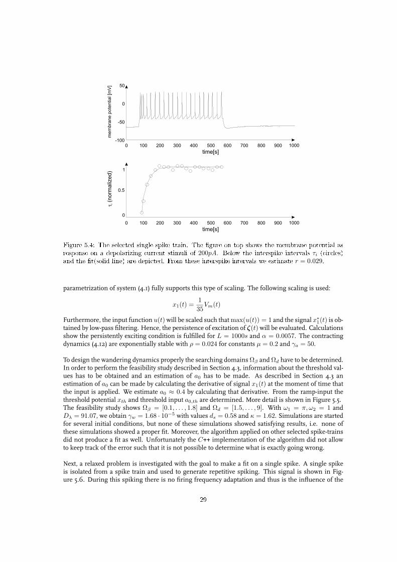
Figure 5.4: The selected single spike train. The gure on top shows the membrane potential asresponse on a depolarizing current stimuli of 200pA. Below the interspike intervals τi (circles)and the t(solid line) are depicted. From these interspike intervals we estimate r = 0.029.
parametrization of system (4.1) fully supports this type of scaling. The following scaling is used:
x1(t) =135
Vm(t)
Furthermore, the input function u(t) will be scaled such that max(u(t)) = 1 and the signal x∗1(t) is ob-tained by low-pass filtering. Hence, the persistence of excitation of ζ(t) will be evaluated. Calculationsshow the persistently exciting condition is fulfilled for L = 1000s and α = 0.0057. The contractingdynamics (4.12) are exponentially stable with ρ = 0.024 for constants µ = 0.2 and γa = 50.
To design the wandering dynamics properly the searching domains Ωβ and Ωd have to be determined.In order to perform the feasibility study described in Section 4.3, information about the threshold val-ues has to be obtained and an estimation of a0 has to be made. As described in Section 4.3 anestimation of a0 can be made by calculating the derivative of signal x1(t) at the moment of time thatthe input is applied. We estimate a0 ≈ 0.4 by calculating that derivative. From the ramp-input thethreshold potential xth and threshold input a0,th are determined. More detail is shown in Figure 5.5.The feasibility study shows Ωβ = [0.1, . . . , 1.8] and Ωd = [1.5, . . . , 9]. With ω1 = π, ω2 = 1 andDλ = 91.07, we obtain γw = 1.68 · 10−5 with values ds = 0.58 and κ = 1.62. Simulations are startedfor several initial conditions, but none of these simulations showed satisfying results, i.e. none ofthese simulations showed a proper fit. Moreover, the algorithm applied on other selected spike-trainsdid not produce a fit as well. Unfortunately the C++ implementation of the algorithm did not allowto keep track of the error such that it is not possible to determine what is exactly going wrong.
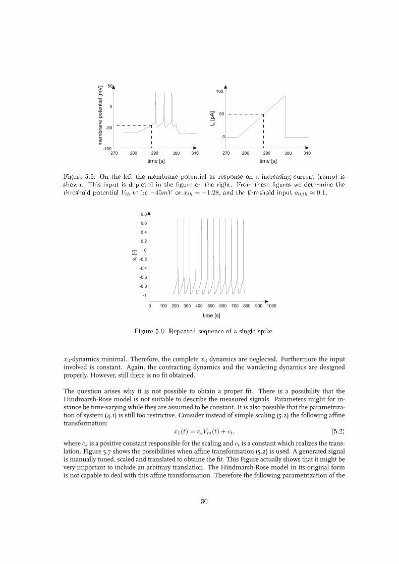
Next, a relaxed problem is investigated with the goal to make a fit on a single spike. A single spikeis isolated from a spike train and used to generate repetitive spiking. This signal is shown in Fig-ure 5.6. During this spiking there is no firing frequency adaptation and thus is the influence of the
29
270 280 290 300 310-100
-50
0
50
time [s]
mem
bra
ne p
ote
ntial [m
V]
0
50
100
I[p
A]
inj
270 280 290 300 310
time [s]
Figure 5.5: On the left the membrane potential as response on a increasing current (ramp) isshown. This input is depicted in the gure on the right. From these gures we determine thethreshold potential Vth to be −45mV or xth = −1.28, and the threshold input a0,th ≈ 0.1.
0 100 200 300 400 500 600 700 800 900 1000
-1
-0.8
-0.6
-0.4
-0.2
0
0.2
0.4
0.6
0.8
x[-
]1
time [s]
Figure 5.6: Repeated sequence of a single spike.
x3-dynamics minimal. Therefore, the complete x3 dynamics are neglected. Furthermore the inputinvolved is constant. Again, the contracting dynamics and the wandering dynamics are designedproperly. However, still there is no fit obtained.
The question arises why it is not possible to obtain a proper fit. There is a possibility that theHindmarsh-Rose model is not suitable to describe the measured signals. Parameters might for in-stance be time-varying while they are assumed to be constant. It is also possible that the parametriza-tion of system (4.1) is still too restrictive. Consider instead of simple scaling (5.2) the following affinetransformation:
x1(t) = csVm(t) + ct, (5.2)where cs is a positive constant responsible for the scaling and ct is a constant which realizes the trans-lation. Figure 5.7 shows the possibilities when affine transformation (5.2) is used. A generated signalis manually tuned, scaled and translated to obtaine the fit. This Figure actually shows that it might bevery important to include an arbitrary translation. The Hindmarsh-Rose model in its original formis not capable to deal with this affine transformation. Therefore the following parametrization of the
30
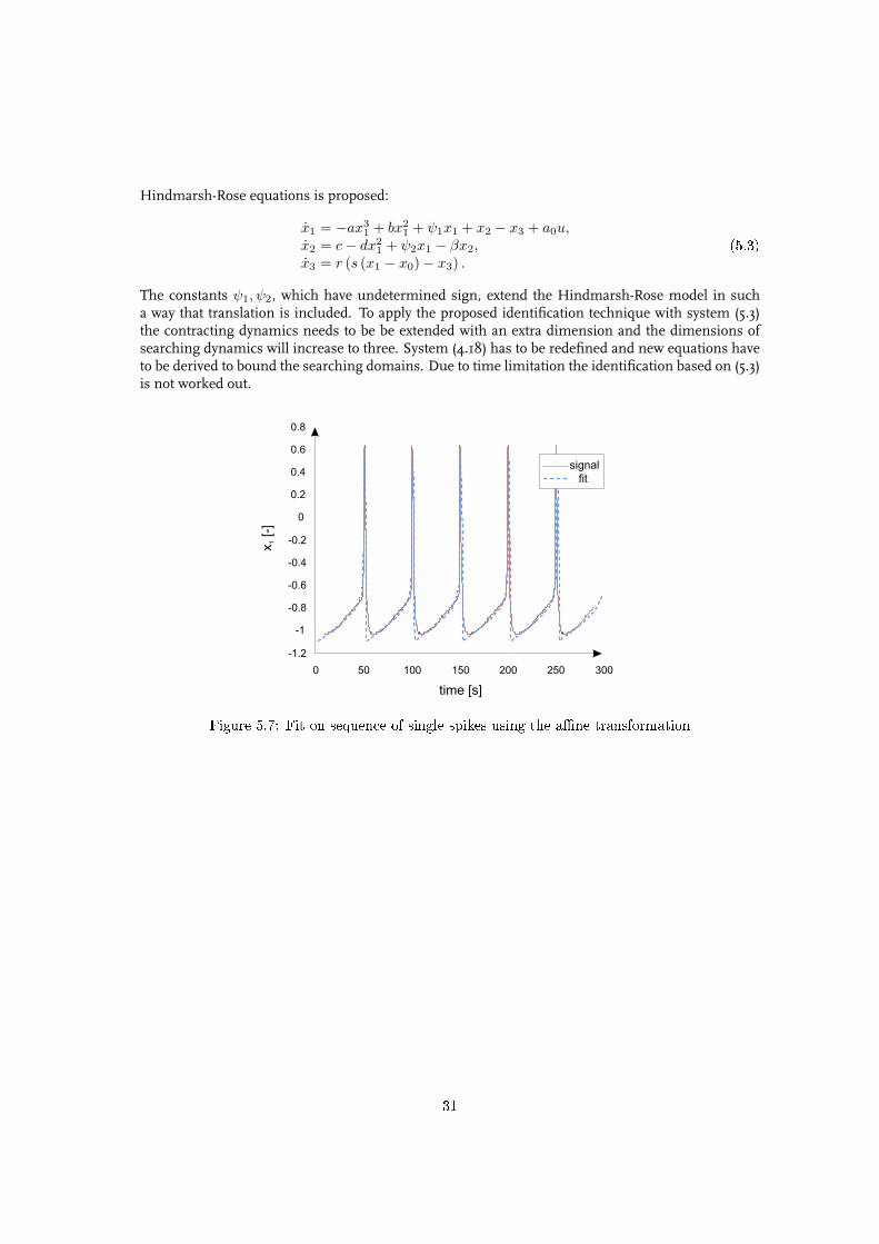
Hindmarsh-Rose equations is proposed:
x1 = −ax31 + bx2
1 + ψ1x1 + x2 − x3 + a0u,x2 = c− dx2
1 + ψ2x1 − βx2,x3 = r (s (x1 − x0)− x3) .
(5.3)
The constants ψ1, ψ2, which have undetermined sign, extend the Hindmarsh-Rose model in sucha way that translation is included. To apply the proposed identification technique with system (5.3)the contracting dynamics needs to be be extended with an extra dimension and the dimensions ofsearching dynamics will increase to three. System (4.18) has to be redefined and new equations haveto be derived to bound the searching domains. Due to time limitation the identification based on (5.3)is not worked out.
0 50 100 150 200 250 300
-1.2
-1
-0.8
-0.6
-0.4
-0.2
0
0.2
0.4
0.6
0.8
time [s]
x[-
]1
signal
fit
Figure 5.7: Fit on sequence of single spikes using the ane transformation
31
Chapter 6
Conclusions and Recommendations
6.1 ConclusionsIn this study a method is described to estimate parameters of a neuronal model. The membranepotential is measured from neurons from the hippocampus of mice in a common current clampedsetup and in a current clamped setup where tonic GABAAreceptors have been blocked by treatingthe neuron with the chemical Picrotoxin. The model to make the fit with was chosen to be theHindmarsh-Rose model. This phase-plane model describes a large number of biophysical featureswith a minimal number of state variables and parameters. The model with the used parametriza-tion did not satisfy the condition of observability and therefore conventional methods like adaptiveobservers could not be used. Without the ability to use conventional identification techniques, a newtechnique making use of contracting and wandering dynamics is presented. The contracting dynam-ics contain parameters that appear linearly in known and measurable signals of the one-dimensionalequivalent of the Hindmarsh-Rose model. With a suitable update law and given that the persis-tently exciting condition does hold, these parameters are estimated correctly and the dynamics of thecontracting part are exponentially stable. The wandering dynamics perform a search in a boundeddomain for parameter values which can not be estimated by the contracting dynamics. The speed ofthe search is mainly determined by the time the contracting dynamics need to reach its steady-state.Furthermore, inequalities are presented which are used to determine the feasible searching domain.Next, the algorithm is implemented in Matlab and C++, from which the C++ implementation turnedout to be about hundred times faster then the Matlab solution.
The algorithm is first successfully tested in simulations with a generated signal from the Hindmarsh-Rose equations. In the case where measured signals are used no fit is obtained. Maybe it is notpossible to fit a Hindmarsh-Rose model on measured membrane potentials since the model does notdeal with time-varying parameter. However, it is more likely that a wrong type of scaling is used.Preliminary results using an affine transformation instead of scaling are promising.
6.2 RecommendationsSince there are strong indications that a fit with the use of an affine transformation is possible, it isrecommended to work out the presented technique with the contracting and wandering dynamicsusing the extended Hindmarsh-Rose model which includes the affine transformation. Therefore newequations need to be derived to obtain a feasible searching domain and the wandering dynamicsneed to be redesigned. Furthermore it might be a better to use a variable step solver, or even a more
32

advanced solver, in the C++ algorithm to increase accuracy. Furthermore it is recommended to extendthe C++ implementation such that it is possible to keep track of the error.
33
Bibliography
[1] Bullock T.H, Bennett M.V.L, Johnston D, Josephson R, Marder E, Fields R.D. The Neuron Docter-ine, REDUX. SCIENCE, vol 310, november 2005.
[2] Chadderton P, Margrie T.W, Hausser M. Integration of quanta in cerebellar granule cells duringsensory processing. Nature, 2004.
[3] Hindmarsh J.L, Rose R.M. A model of neuronal bursting using three coupled first order differntialequations. Proc. R. Soc. Lond. B 221, 87-102, 1984.
[4] Hindmarsh J.L, Cornelius P. The Development of the Hindmarsh-Rose model for bursting. BURST-ING: The Genesis of Rhythm in the Nervous System, CH 1, 2005.
[5] Hodgkin A.L, Huxley A.F. A quantitative description of membrane current and its application toconductionand excitation in nerve. J.Physol 117, 500-544, 1952.
[6] Izhikevich E.M. Which Model to Use for Cortical Spiking Neurons? IEEE trans. on neural networks,september 2004.
[7] Khalil H.K. Nonlinear Systems. Prentice Hall, 2002.
[8] Kreisselmeier G. Adaptive Observers with Exponential Rate of Convergence. IEEE trans. on Auto-matic Control, vol. ac-22, no.1, february 1977.
[9] Koch C. Biophysics of computation. Oxford University Press, 1999.
[10] Lamsa K, Heeroma J.H, Kullmann D.M. Hebbian LTP in feed-forward inhibitory interneurons andthe temporal fidelity of input discrimination. Nat Neurosci, 2005.
[11] London M, Hausser M. Dendritic computation. Annu Rev Neurosci, 2005.
[12] Loría A. Explicit convergenve rates for MRAC-type systems. Automatica, september 2003.
[13] Loría A, Panteley E. Uniform exponential stability of linear time-varying systems: revisited. Systems& Control Letters 47, 13-24, 2002.
[14] Marino R. Adaptive Observers for Single Output Nonlinear Systems. IEEE trans. on Automatic Con-trol, vol. 35, no.9, september 1990.
[15] Marino R, Tomei P. Global Adaptive Observers for Nonlinear Systems via Filtered Transformations.IEEE trans. on Automatic Control, vol. 37, no.8, august 1992.
[16] Mitchell S.J, Silver R.A. Shunting inhibition modulates neuronal gain during synaptic excitation.Neuron, 2003.
34

[17] Morgan A.P, Narendra K.S. On the stability of nonautonomous differential equations x = [A +B(t)]x with skew symmetric matrix B(t)∗. SIAM J. Control and Optimization, Vol. 15, No.1, Jan-uary 1977.
[18] Pouille F, Scanziani M. Enforcement of temporal fidelity in pyramidal cells by somatic feed-forwardinhibition. Science, 2001.
[19] Semyanov A, Walker M.C, Kullmann D.M, Silver R.A. Tonically active GABA A receptors: modu-lating gain and maintaining the tone. Trends Neurosci, 2004.
[20] Tyukin I.Y, Prokorov D.V., van Leeuwen C. Adaptation and Parameter Estima-tion in Systems with Unstable Target Dynamics and Nonlinear Parametrization.http://arxiv.org/abs/math.OC/0506419, 2005.
[21] Tyukin I.Y, Steur E, Nijmeijer H, van Leeuwen C. Non-uniform Attractivity, Meta-stability andSmall-gain Theorems. preprint (2006).
35
Appendix A
Gains Df,β and Df,d
In this appendix, analytical expressions for the gain Df,β and Df,d in (4.16) are presented. The errorin x1(t) caused by errors in the parameters β and d is given by:
f(β, d, t)− f(β, d, t) =(f(β, d, t)− f(β, d, t)
)
+(f(β, d, t)− f(β, d, t)
), (A.1)
where
x2(t) = e−βtx2(t = 0) +
t∫
0
e−β(t−τ)dx21(τ)dτ. (A.2)
The first part of the righthand side of (A.2) is monotonic decreasing with respect to the time, and itsvalue is assumed to be small. Therefore, this part will be neglected in further analysis. Given x(t) isbounded, f(β, d, t)− f(β, d, t) will be bounded by the following expression:
d ‖ x21(τ) ‖∞,[t0,t]
t∫
0
(e−β(t−τ) − e−θ1(t−τ)
)dτ. (A.3)
With the use of Hadamard’s lemma, (A.3) can be explicitly written as some function Df,β(·) mul-tiplied by (β − β). Therefore, introduce β? ∈ [β, β] and a dimensionless number ς ∈ [0, 1] suchthat
β? = ςβ + (1− ς)β (A.4)Equations (A.2) and (A.4) can be combined to the following expression:
d ‖ x21(τ) ‖∞,[t0,t]
(1∫0
∂∂β?
(t∫0
e−β?(t−τ)∂τ
)∂ν
)(β − β)
= d ‖ x21(τ) ‖∞,[t0,t]
(1∫0
∂∂β?
(1
β?
(1− e−β?t
))∂ν
)(β − β)
= d ‖ x21(τ) ‖∞,[t0,t]
(−1ββ
+ βeβt−βeβt
ββ(β−β)e(β+β)t
)(β − β)
= Df,β(β, β, d, t)(β − β).
36
Denoting the monotonically decreasing part of Df,β by εβ(t), it is easy to see |f(β, d, t) − f(β, d, t)|will be upperbounded by
Df,β |β − β|+ εβ(t), (A.5)
where
Df,β =(
d
ββ
)‖ x2
1(τ) ‖∞,[t0,t] .
Using the same approach, the bounds of f(β, d, t) − f(β, d, t) will be derived. Let us again neglectthe monotonically decreasing terms, such that the following expression holds:
t∫0
(e−β(t−τ)
)(d− d)x2
1(τ)dτ
≤t∫0
(e−β(t−τ)
)dτ(d− d) ‖ x2
1(τ) ‖∞,[t0,t] .
It is straightforward that (A.6) can be bounded from above by
Df,d|d− d|+ εd(t), (A.6)
where
Df,d =1
β‖ x2
1(τ) ‖∞,[t0,t]
and εd(t) is a monotonically decreasing function in time.
37
Appendix B
Recorded Signals
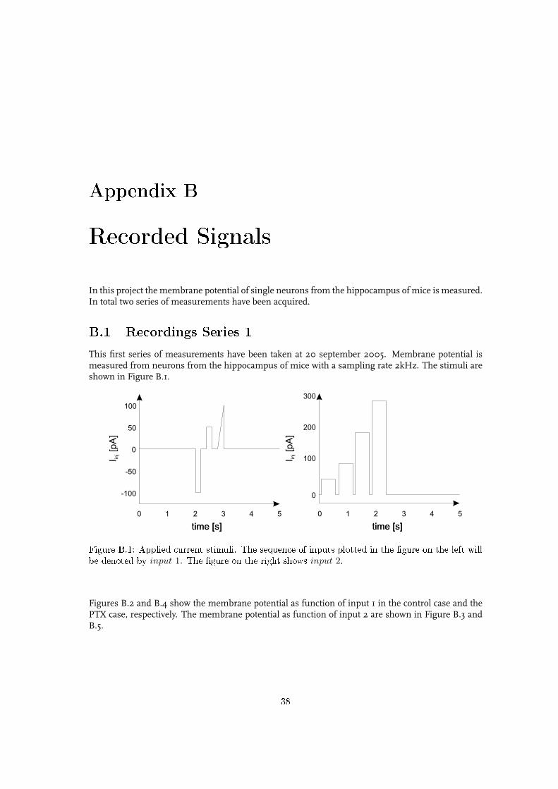
In this project the membrane potential of single neurons from the hippocampus of mice is measured.In total two series of measurements have been acquired.
B.1 Recordings Series 1This first series of measurements have been taken at 20 september 2005. Membrane potential ismeasured from neurons from the hippocampus of mice with a sampling rate 2kHz. The stimuli areshown in Figure B.1.
0 1 2 3 4 5
-100
-50
0
50
100
time [s]time [s]
I[p
A]
inj
0
100
200
300
0 1 2 3 4 5
time [s]time [s]
I[p
A]
inj
Figure B.1: Applied current stimuli. The sequence of inputs plotted in the gure on the left willbe denoted by input 1. The gure on the right shows input 2.
Figures B.2 and B.4 show the membrane potential as function of input 1 in the control case and thePTX case, respectively. The membrane potential as function of input 2 are shown in Figure B.3 andB.5.
38

0 1 2 3 4 5
-100
-80
-60
-40
-20
0
20
40
me
mb
ran
e p
ote
ntia
l [m
V]
time [s]
-100
-80
-60
-40
-20
0
20
40
me
mb
ran
e p
ote
ntia
l [m
V]
0 1 2 3 4 5
time [s]
0 1 2 3 4 5
time [s]
-100
-80
-60
-40
-20
0
20
40
mem
bra
ne p
ote
ntial [m
V]
0 1 2 3 4 5
time [s]
-100
-80
-60
-40
-20
0
20
40
mem
bra
ne p
ote
ntial [m
V]
-80
-60
-40
-20
0
20
40
mem
bra
ne p
ote
ntial [m
V]
-100
0 1 2 3 4 5
time [s]
-80
-60
-40
-20
0
20
40
me
mb
ran
e p
ote
ntia
l [m
V]
-100
0 1 2 3 4 5
time [s]
-80
-60
-40
-20
0
20
40
mem
bra
ne p
ote
ntial [m
V]
-100
0 1 2 3 4 5
time [s]
-80
-60
-40
-20
0
20
40
me
mb
ran
e p
ote
ntia
l [m
V]
-100
0 1 2 3 4 5
time [s]
-80
-60
-40
-20
0
20
40
me
mb
ran
e p
ote
ntia
l [m
V]
-100
0 1 2 3 4 5
time [s]
-80
-60
-40
-20
0
20
40
mem
bra
ne p
ote
ntial [m
V]
-100
0 1 2 3 4 5
time [s]
Figure B.2: Control, input 1.
39
-80
-60
-40
-20
0
20
40
me
mb
ran
e p
ote
ntia
l [m
V]
0 1 2 3 4 5
time [s]
-80
-60
-40
-20
0
20
40
mem
bra
ne p
ote
ntial [m
V]
0 1 2 3 4 5
time [s]
-80
-60
-40
-20
0
20
40
mem
bra
ne p
ote
ntial [m
V]
0 1 2 3 4 5
time [s]
-80
-60
-40
-20
0
20
40
mem
bra
ne p
ote
ntial [m
V]
0 1 2 3 4 5
time [s]
-80
-60
-40
-20
0
20
40
me
mb
ran
e p
ote
ntia
l [m
V]
0 1 2 3 4 5
time [s]
-80
-60
-40
-20
0
20
40
mem
bra
ne p
ote
ntial [m
V]
0 1 2 3 4 5
time [s]
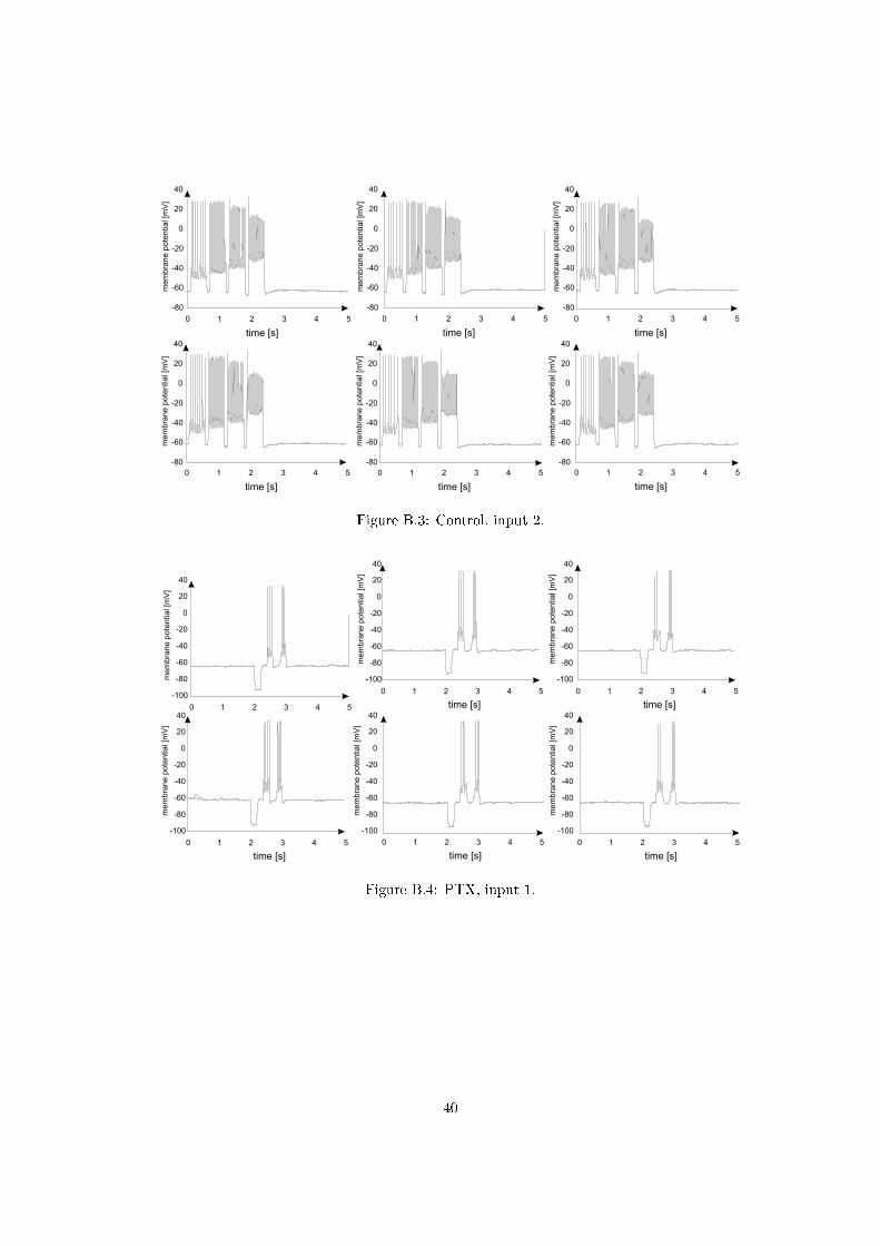
Figure B.3: Control, input 2.
0 1 2 3 4 5
-100
-80
-60
-40
-20
0
20
40
mem
bra
ne p
ote
ntial [m
V]
-100
-80
-60
-40
-20
0
20
40
mem
bra
ne p
ote
ntial [m
V]
0 1 2 3 4 5
time [s]
-100
-80
-60
-40
-20
0
20
40
me
mb
ran
e p
ote
ntia
l [m
V]
0 1 2 3 4 5
time [s]
-100
-80
-60
-40
-20
0
20
40
mem
bra
ne p
ote
ntial [m
V]
0 1 2 3 4 5
time [s]
0 1 2 3 4 5
time [s]
-100
-80
-60
-40
-20
0
20
40
mem
bra
ne p
ote
ntial [m
V]
0 1 2 3 4 5
time [s]
-100
-80
-60
-40
-20
0
20
40
mem
bra
ne p
ote
ntial [m
V]
Figure B.4: PTX, input 1.
40
0 1 2 3 4 5
-80
-60
-40
-20
0
20
40
mem
bra
ne p
ote
ntial [m
V]
time [s]
-80
-60
-40
-20
0
20
40
me
mb
ran
e p
ote
ntia
l [m
V]
0 1 2 3 4 5
time [s]
-80
-60
-40
-20
0
20
40
mem
bra
ne p
ote
ntial [m
V]
0 1 2 3 4 5
time [s]
-80
-60
-40
-20
0
20
40
mem
bra
ne p
ote
ntial [m
V]
0 1 2 3 4 5
time [s]
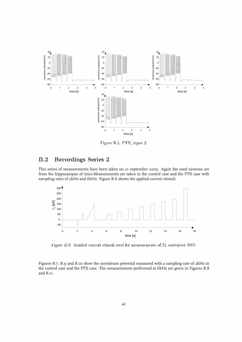
Figure B.5: PTX, input 2.
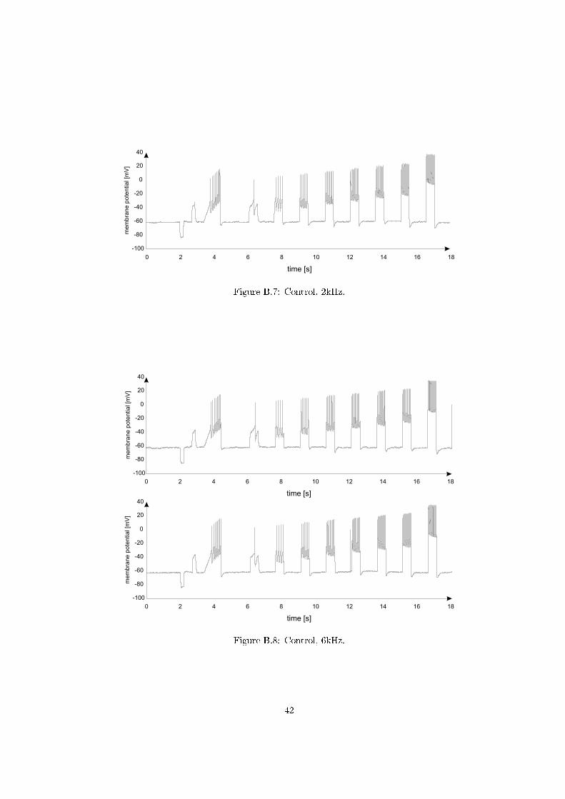
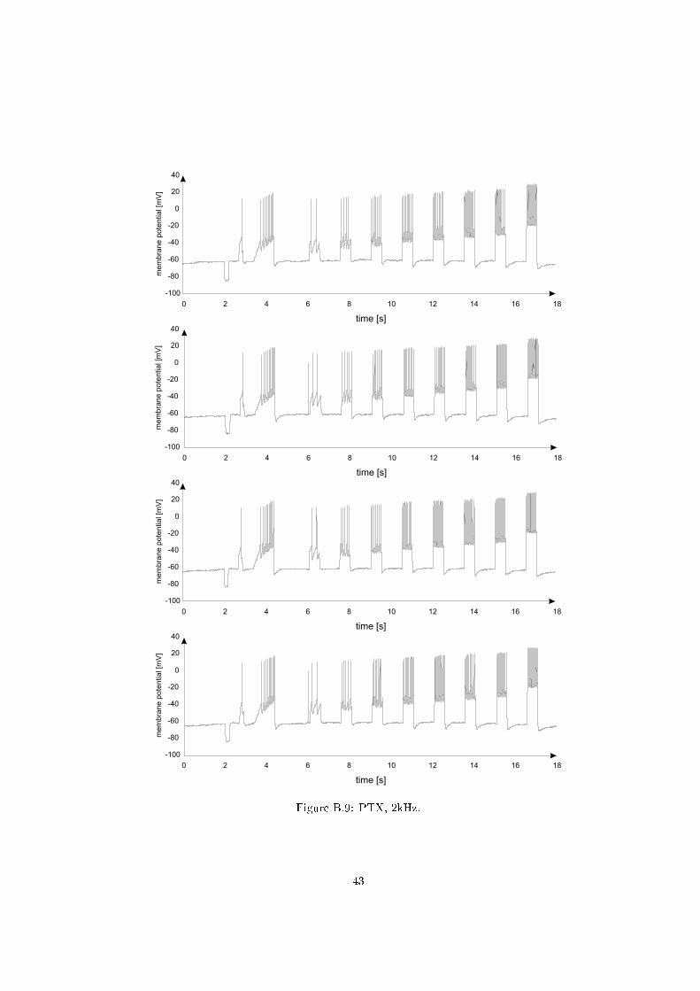
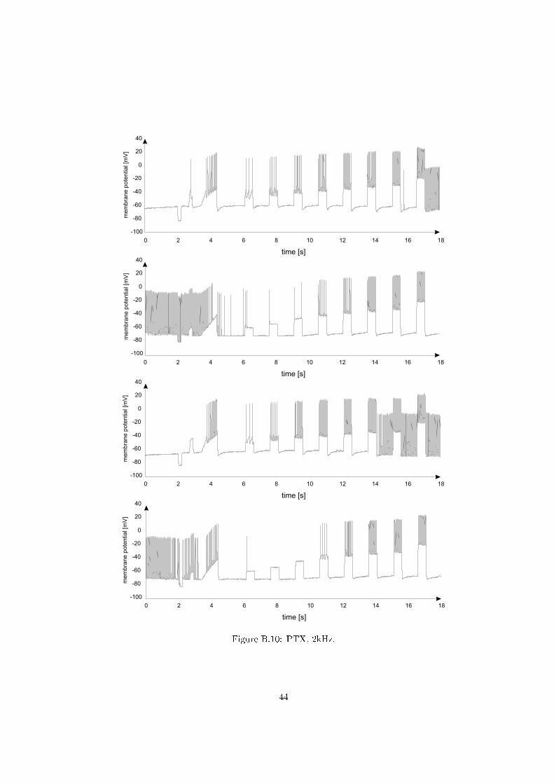
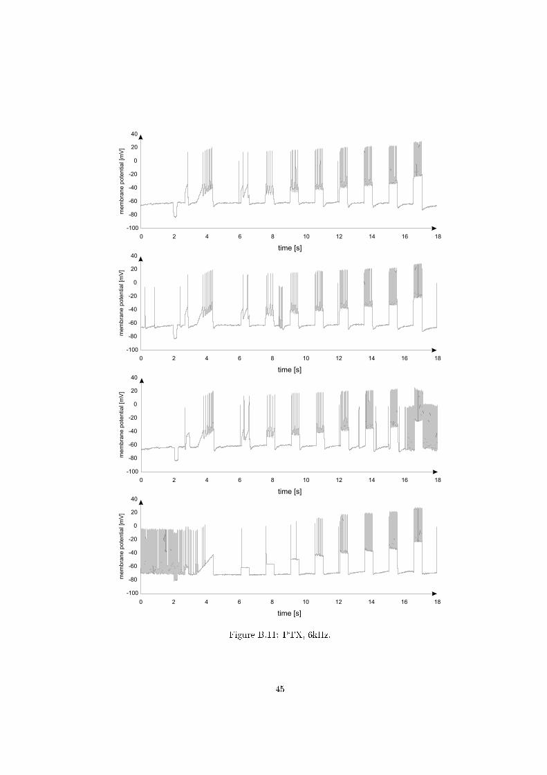
B.2 Recordings Series 2This series of measurements have been taken on 21 september 2005. Again the used neurons arefrom the hippocampus of mice.Measurements are taken in the control case and the PTX case withsampling rates of 2kHz and 6kHz. Figure B.6 shows the applied current stimuli.
0 2 4 6 8 10 12 14 16 18
-50
0
50
100
150
200
250
300
time [s]
I[p
A]
inj
Figure B.6: Applied current stimuli used for measurements of 21 september 2005.
Figures B.7, B.9 and B.10 show the membrane potential measured with a sampling rate of 2kHz inthe control case and the PTX case. The measurements performed at 6kHz are given in Figures B.8and B.11.
41
0 2 4 6 8 10 12 14 16 18
-100
-80
-60
-40
-20
0
20
40
me
mb
ran
e p
ote
ntia
l [m
V]
time [s]
Figure B.7: Control, 2kHz.
0 2 4 6 8 10 12 14 16 18
time [s]
-100
-80
-60
-40
-20
0
20
40
me
mb
ran
e p
ote
ntia
l [m
V]
0 2 4 6 8 10 12 14 16 18
time [s]
-100
-80
-60
-40
-20
0
20
40
me
mb
ran
e p
ote
ntia
l [m
V]
Figure B.8: Control, 6kHz.
42
0 2 4 6 8 10 12 14 16 18
-100
-80
-60
-40
-20
0
20
40
me
mb
ran
e p
ote
ntia
l [m
V]
time [s]
-100
-80
-60
-40
-20
0
20
40
me
mb
ran
e p
ote
ntia
l [m
V]
0 2 4 6 8 10 12 14 16 18
time [s]
-100
-80
-60
-40
-20
0
20
40
me
mb
ran
e p
ote
ntia
l [m
V]
0 2 4 6 8 10 12 14 16 18
time [s]
-100
-80
-60
-40
-20
0
20
40
me
mb
ran
e p
ote
ntia
l [m
V]
0 2 4 6 8 10 12 14 16 18
time [s]
Figure B.9: PTX, 2kHz.
43
-100
-80
-60
-40
-20
0
20
40
me
mb
ran
e p
ote
ntia
l [m
V]
0 2 4 6 8 10 12 14 16 18
time [s]
-100
-80
-60
-40
-20
0
20
40
me
mb
ran
e p
ote
ntia
l [m
V]
0 2 4 6 8 10 12 14 16 18
time [s]
-100
-80
-60
-40
-20
0
20
40
me
mb
ran
e p
ote
ntia
l [m
V]
0 2 4 6 8 10 12 14 16 18
time [s]
-100
-80
-60
-40
-20
0
20
40
me
mb
ran
e p
ote
ntia
l [m
V]
0 2 4 6 8 10 12 14 16 18
time [s]
Figure B.10: PTX, 2kHz.
44
0 2 4 6 8 10 12 14 16 18
-100
-80
-60
-40
-20
0
20
40
me
mb
ran
e p
ote
ntia
l [m
V]
time [s]
-100
-80
-60
-40
-20
0
20
40
me
mb
ran
e p
ote
ntia
l [m
V]
0 2 4 6 8 10 12 14 16 18
time [s]
-100
-80
-60
-40
-20
0
20
40
me
mb
ran
e p
ote
ntia
l [m
V]
0 2 4 6 8 10 12 14 16 18
time [s]
-100
-80
-60
-40
-20
0
20
40
me
mb
ran
e p
ote
ntia
l [m
V]
0 2 4 6 8 10 12 14 16 18
time [s]
Figure B.11: PTX, 6kHz.
45
Appendix C
Numerical Algorithm
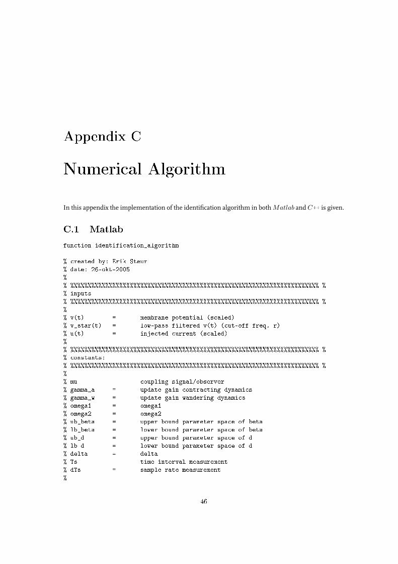
In this appendix the implementation of the identification algorithm in both Matlab and C++ is given.
C.1 Matlabfunction identification_algorithm
% created by: Erik Steur% date: 26-okt-2005%% %%%%%%%%%%%%%%%%%%%%%%%%%%%%%%%%%%%%%%%%%%%%%%%%%%%%%%%%%%%%%%%%%%%%%%% %% inputs% %%%%%%%%%%%%%%%%%%%%%%%%%%%%%%%%%%%%%%%%%%%%%%%%%%%%%%%%%%%%%%%%%%%%%%% %%% v(t) = membrane potential (scaled)% v_star(t) = low-pass filtered v(t) (cut-off freq. r)% u(t) = injected current (scaled)%% %%%%%%%%%%%%%%%%%%%%%%%%%%%%%%%%%%%%%%%%%%%%%%%%%%%%%%%%%%%%%%%%%%%%%%% %% constants:% %%%%%%%%%%%%%%%%%%%%%%%%%%%%%%%%%%%%%%%%%%%%%%%%%%%%%%%%%%%%%%%%%%%%%%% %%% mu = coupling signal/observer% gamma_a = update gain contracting dynamics% gamma_w = update gain wandering dynamics% omega1 = omega1% omega2 = omega2% ub_beta = upper bound parameter space of beta% lb_beta = lower bound parameter space of beta% ub_d = upper bound parameter space of d% lb_d = lower bound parameter space of d% delta = delta% Ts = time interval measurement% dTs = sample rate measurement%
46

% %%%%%%%%%%%%%%%%%%%%%%%%%%%%%%%%%%%%%%%%%%%%%%%%%%%%%%%%%%%%%%%%%%%%%%% %
% generalclear all;close all;clc
global mu gamma_a gamma_w omega_1 omega_2 ub_beta lb_beta ub_d lb_d ...delta Ts dTs
% read dataload data
% assign parameter valuesmu =gamma_a =gamma_w =omega_1 =omega_2 =ub_beta =lb_beta =ub_d =lb_d =delta =Ts =dTs =
% initial conditionsa0 =b0 =nu0 =s0 =a00 =x0 =y0 =
X0 = [x0; y0; a0; b0; nu0; s0; a00];
% generate solutionTspan = [];
[Tout Xout] = ode23(@id_alg,Tspan,[X0;[1;0;1;0]]);
save Iddata Tout Xout
% %%%%%%%%%%%%%%%%%%%%%%%%%%%%%%%%%%%%%%%%%%%%%%%%%%%%%%%%%%%%%%%%%%%%%%% %function dx = id_alg(t,x)
global mu gamma_a gamma_w omega_1 omega_2 ub_beta lb_beta ub_d lb_d ...delta Ts dTs
dx = zeros(11,1);
47
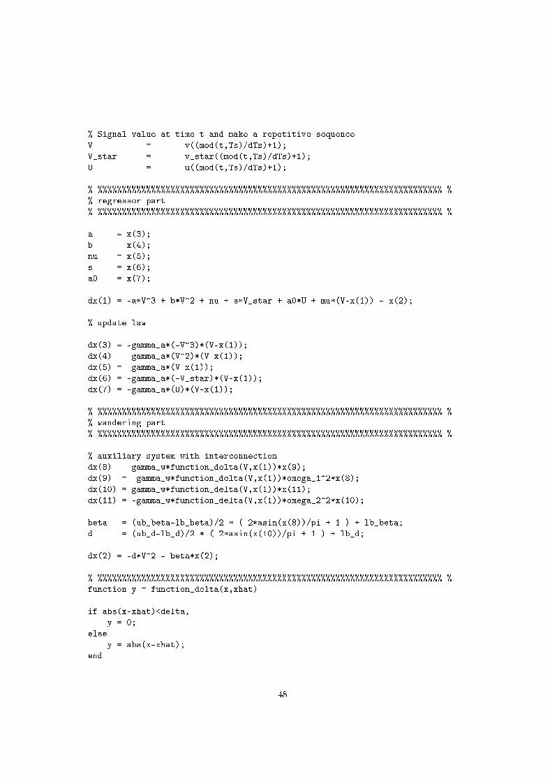
% Signal value at time t and make a repetitive sequenceV = v((mod(t,Ts)/dTs)+1);V_star = v_star((mod(t,Ts)/dTs)+1);U = u((mod(t,Ts)/dTs)+1);
% %%%%%%%%%%%%%%%%%%%%%%%%%%%%%%%%%%%%%%%%%%%%%%%%%%%%%%%%%%%%%%%%%%%%%%% %% regressor part% %%%%%%%%%%%%%%%%%%%%%%%%%%%%%%%%%%%%%%%%%%%%%%%%%%%%%%%%%%%%%%%%%%%%%%% %
a = x(3);b = x(4);nu = x(5);s = x(6);a0 = x(7);
dx(1) = -a*V^3 + b*V^2 + nu + s*V_star + a0*U + mu*(V-x(1)) - x(2);
% update law
dx(3) = -gamma_a*(-V^3)*(V-x(1));dx(4) = -gamma_a*(V^2)*(V-x(1));dx(5) = -gamma_a*(V-x(1));dx(6) = -gamma_a*(-V_star)*(V-x(1));dx(7) = -gamma_a*(U)*(V-x(1));
% %%%%%%%%%%%%%%%%%%%%%%%%%%%%%%%%%%%%%%%%%%%%%%%%%%%%%%%%%%%%%%%%%%%%%%% %% wandering part% %%%%%%%%%%%%%%%%%%%%%%%%%%%%%%%%%%%%%%%%%%%%%%%%%%%%%%%%%%%%%%%%%%%%%%% %
% auxiliary system with interconnectiondx(8) = gamma_w*function_delta(V,x(1))*x(9);dx(9) = -gamma_w*function_delta(V,x(1))*omega_1^2*x(8);dx(10) = gamma_w*function_delta(V,x(1))*x(11);dx(11) = -gamma_w*function_delta(V,x(1))*omega_2^2*x(10);
beta = (ub_beta-lb_beta)/2 * ( 2*asin(x(8))/pi + 1 ) + lb_beta;d = (ub_d-lb_d)/2 * ( 2*asin(x(10))/pi + 1 ) + lb_d;
dx(2) = -d*V^2 - beta*x(2);
% %%%%%%%%%%%%%%%%%%%%%%%%%%%%%%%%%%%%%%%%%%%%%%%%%%%%%%%%%%%%%%%%%%%%%%% %function y = function_delta(x,xhat)
if abs(x-xhat)<delta,y = 0;
elsey = abs(x-xhat);
end
48
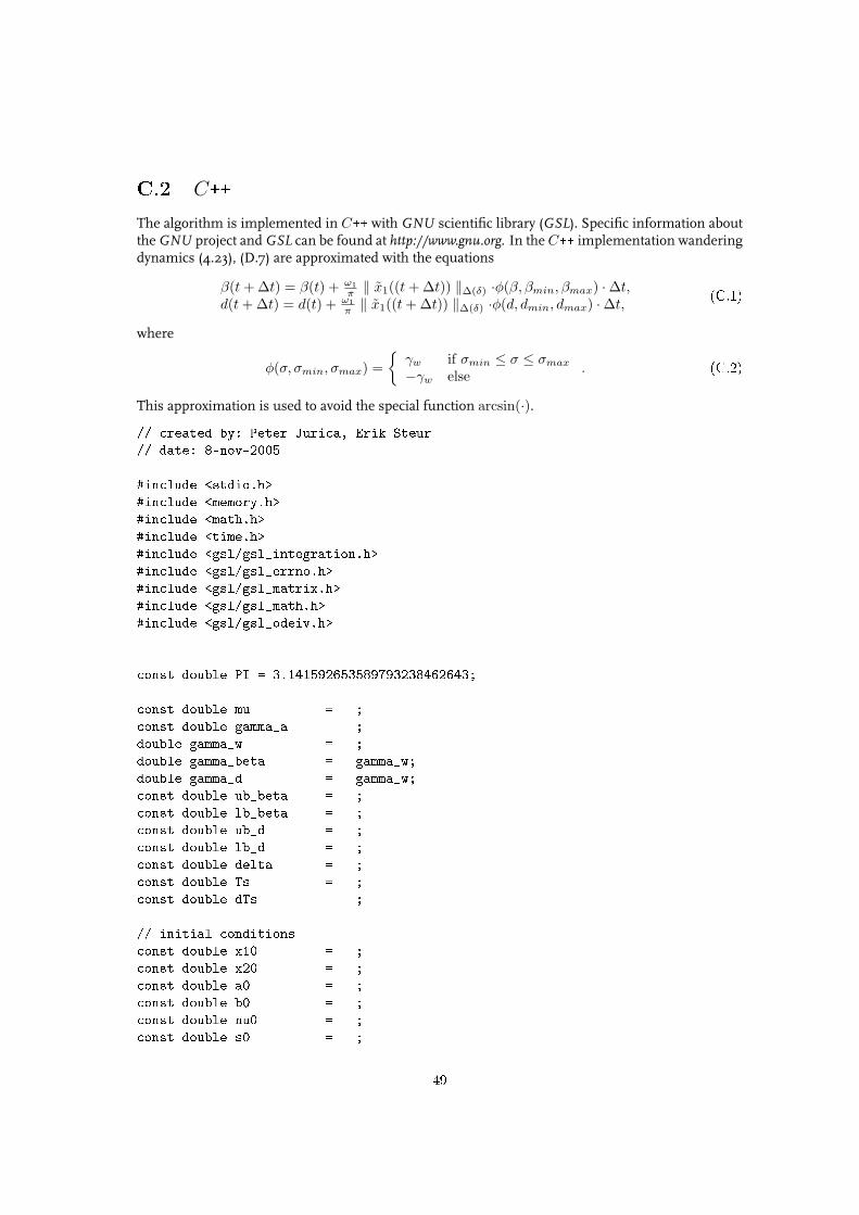
C.2 C++The algorithm is implemented in C++ with GNU scientific library (GSL). Specific information aboutthe GNU project and GSL can be found at http://www.gnu.org. In the C++ implementation wanderingdynamics (4.23), (D.7) are approximated with the equations
β(t + ∆t) = β(t) + ω1π ‖ x1((t + ∆t)) ‖∆(δ) ·φ(β, βmin, βmax) ·∆t,
d(t + ∆t) = d(t) + ω1π ‖ x1((t + ∆t)) ‖∆(δ) ·φ(d, dmin, dmax) ·∆t,
(C.1)
where
φ(σ, σmin, σmax) =
γw if σmin ≤ σ ≤ σmax
−γw else . (C.2)
This approximation is used to avoid the special function arcsin(·).// created by: Peter Jurica, Erik Steur// date: 8-nov-2005
#include <stdio.h>#include <memory.h>#include <math.h>#include <time.h>#include <gsl/gsl_integration.h>#include <gsl/gsl_errno.h>#include <gsl/gsl_matrix.h>#include <gsl/gsl_math.h>#include <gsl/gsl_odeiv.h>
const double PI = 3.141592653589793238462643;
const double mu = ;const double gamma_a = ;double gamma_w = ;double gamma_beta = gamma_w;double gamma_d = gamma_w;const double ub_beta = ;const double lb_beta = ;const double ub_d = ;const double lb_d = ;const double delta = ;const double Ts = ;const double dTs = ;
// initial conditionsconst double x10 = ;const double x20 = ;const double a0 = ;const double b0 = ;const double nu0 = ;const double s0 = ;
49
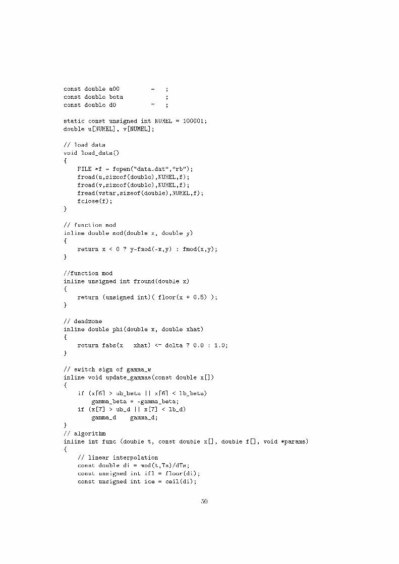
const double a00 = ;const double beta = ;const double d0 = ;
static const unsigned int NUMEL = 100001;double u[NUMEL], v[NUMEL];
// load datavoid load_data()
FILE *f = fopen("data.dat","rb");fread(u,sizeof(double),NUMEL,f);fread(v,sizeof(double),NUMEL,f);fread(vstar,sizeof(double),NUMEL,f);fclose(f);
// function modinline double mod(double x, double y)
return x < 0 ? y-fmod(-x,y) : fmod(x,y);
//function modinline unsigned int fround(double x)
return (unsigned int)( floor(x + 0.5) );
// deadzoneinline double phi(double x, double xhat)
return fabs(x - xhat) <= delta ? 0.0 : 1.0;
// switch sign of gamma_winline void update_gammas(const double x[])
if (x[6] > ub_beta || x[6] < lb_beta)gamma_beta = -gamma_beta;
if (x[7] > ub_d || x[7] < lb_d)gamma_d = -gamma_d;
// algorithminline int func (double t, const double x[], double f[], void *params)
// linear interpolationconst double di = mod(t,Ts)/dTs;const unsigned int ifl = floor(di);const unsigned int ice = ceil(di);
50
const double V = v[ifl] + (v[ice] - v[ifl])*(di-ifl);const double U = u[ifl] + (u[ice] - u[ifl])*(di-ifl);const double Vstar = vstar[ifl] + (vstar[ice] - vstar[ifl])*(di-ifl);
const double a = x[1];const double b = x[2];const double nu = x[3];const double s = x[4];const double a0 = x[5];
const double aVx0 = fabs((V-x[0]));const double pVx0 = phi(V,x[0]);const double V2 = V*V;const double V3 = V*V2;
f[0] = -a*V3 + b*V2 + x[8] - s*Vstar + nu + a0*U + mu*(V-x[0]);
f[1] = gamma_a*(-V3)*(V-x[0]);f[2] = gamma_a*V2*(V-x[0]);f[3] = gamma_a*(V-x[0]);f[4] = gamma_a*(-Vstar)*(V-x[0]);f[5] = gamma_a*U*(V-x[0]);
update_gammas(x);f[6] = -gamma_beta*aVx0*pVx0;f[7] = -gamma_d*aVx0*pVx0;
f[8] = -x[7]*V2 - x[6]*x[8];
return GSL_SUCCESS;// solverint main_fixed(double* X0)
const gsl_odeiv_step_type * T = gsl_odeiv_step_rk2;gsl_odeiv_step * s = gsl_odeiv_step_alloc (T, 10);gsl_odeiv_system sys = func, NULL, 10, NULL;
double t = 0, t1 = 100;//1000;double h = 1e-3;double y[10], y_err[10];memcpy(y, X0, 10*sizeof(double));double dydt_in[10], dydt_out[10];
GSL_ODEIV_FN_EVAL(&sys, t, y, dydt_in);
51
FILE* fout = NULL;fclose(fopen("simlog.dat","wb"));double trec_start, elapsed;time_t start, finish;time(&start);int count = 0;while (true) ///(t < t1)
int status = gsl_odeiv_step_apply (s, t, h,y, y_err,dydt_in,dydt_out,&sys);
if (status != GSL_SUCCESS)break;
memcpy(dydt_in, dydt_out, 10*sizeof(double));
t += h;count++;if (count%10 == 0)
if (fout != NULL)
fwrite(&t,sizeof(double),1,fout);fwrite(y,sizeof(double),10,fout);
if (t >= trec_start + 10.0)
fclose(fout);fout = NULL;
if (count == (int)(10.0*1.0/h))
char flag = 0;FILE * f = fopen("plotme.txt","rt");fread(&flag,sizeof(char),1,f);fclose(f);if (flag == '1')
f = fopen("plotme.txt","wt");fprintf(f,"0");fclose(f);
fout = fopen("res.dat","wb");trec_start = t;
52
count = 0;
time(&finish);elapsed = difftime(finish,start);if (elapsed > 600.0)
f = fopen("simlog.dat","ab");fwrite(&t,sizeof(double),1,f);fwrite(y,sizeof(double),10,f);fwrite(&gamma_beta,sizeof(double),1,f);fwrite(&gamma_w,sizeof(double),1,f);fclose(f);
time(&start);
fclose(fout);
gsl_odeiv_step_free (s);return 0;
int main(void)
load_data();
double X0[] = x10,a0,b0,nu0,s0,a00,beta0,d0,x20 ; // 9 states
int ret = main_fixed(X0);
return ret;
53

Appendix D
Non-uniform Attractivity, Meta-stabilityand Small-gain Theorems
Ivan Tyukin1 Erik Steur2, Henk Nijmeijer 3, Cees van Leeuwen4
November 24, 2005 (preprint version)
abstract
This paper addresses a problem of asymptotic, yet non-uniform in initial conditions, convergence ofstate of dynamical systems into a given domain of their state space. The necessity to consider non-uniform convergence arises when either the system itself is inherently globally unstable (intermittent,itinerant, or meta-stable) or the problem statements make stable solution impossible (general opti-mization problems, nonlinear parameter identification and adaptation). Conventional techniques foranalysis of convergence to Lyapunov-unstable equilibria, usually rely on detailed knowledge of theproperties of the vector-fields of systems or a-priori assume boundeness of the state. In contrast tothese we propose a method that does not require boundedness a-priori and relies only on qualitativeinformation about the system dynamics. This information are mere estimates of the input-outputmaps, steady-state characteristics and decomposability into the interconnection of stable, contractingcompartment and unstable, exploratory part. The method can be applied to problems of analysisasymptotic behavior of locally instable systems and systems in the vicinity of attractor ruins, pa-rameter identification and non-dominating adaptation in the presence of nonlinear parametrization.Applications in the design and analysis of models for visual detection and recognition are discussed.
Keywords: non-uniform convergence, small-gain, input-output stability
1Corresponding author. Laboratory for Perceptual Dynamics, RIKEN (Institute for Physical and Chem-ical Research) Brain Science Institute, 2-1, Hirosawa, Wako-shi, Saitama, 351-0198, Japan, e-mail: [email protected]
2Dept. of Mechanical Engineering, Technical University of Eindhoven, The Netherlands3Dept. of Mechanical Engineering, Technical University of Eindhoven, The Netherlands4Laboratory for Perceptual Dynamics, RIKEN (Institute for Physical and Chemical Research) Brain Science
Institute, 2-1, Hirosawa, Wako-shi, Saitama, 351-0198, Japan, e-mail: [email protected]
54
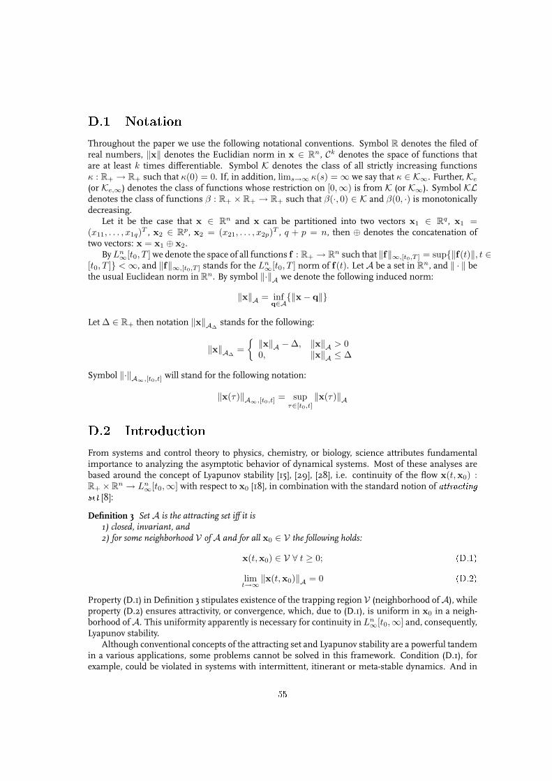
D.1 NotationThroughout the paper we use the following notational conventions. Symbol R denotes the filed ofreal numbers, ‖x‖ denotes the Euclidian norm in x ∈ Rn, Ck denotes the space of functions thatare at least k times differentiable. Symbol K denotes the class of all strictly increasing functionsκ : R+ → R+ such that κ(0) = 0. If, in addition, lims→∞ κ(s) = ∞ we say that κ ∈ K∞. Further, Ke
(or Ke,∞) denotes the class of functions whose restriction on [0,∞) is from K (or K∞). Symbol KLdenotes the class of functions β : R+ × R+ → R+ such that β(·, 0) ∈ K and β(0, ·) is monotonicallydecreasing.
Let it be the case that x ∈ Rn and x can be partitioned into two vectors x1 ∈ Rq , x1 =(x11, . . . , x1q)T , x2 ∈ Rp, x2 = (x21, . . . , x2p)T , q + p = n, then ⊕ denotes the concatenation oftwo vectors: x = x1 ⊕ x2.
By Ln∞[t0, T ] we denote the space of all functions f : R+ → Rn such that ‖f‖∞,[t0,T ] = sup‖f(t)‖, t ∈
[t0, T ] < ∞, and ‖f‖∞,[t0,T ] stands for the Ln∞[t0, T ] norm of f(t). Let A be a set in Rn, and ‖ · ‖ be
the usual Euclidean norm in Rn. By symbol ‖·‖A we denote the following induced norm:
‖x‖A = infq∈A
‖x− q‖
Let ∆ ∈ R+ then notation ‖x‖A∆stands for the following:
‖x‖A∆=
‖x‖A −∆, ‖x‖A > 00, ‖x‖A ≤ ∆
Symbol ‖·‖A∞,[t0,t] will stand for the following notation:
‖x(τ)‖A∞,[t0,t] = supτ∈[t0,t]
‖x(τ)‖A
D.2 IntroductionFrom systems and control theory to physics, chemistry, or biology, science attributes fundamentalimportance to analyzing the asymptotic behavior of dynamical systems. Most of these analyses arebased around the concept of Lyapunov stability [15], [29], [28], i.e. continuity of the flow x(t,x0) :R+ ×Rn → Ln
∞[t0,∞] with respect to x0 [18], in combination with the standard notion of attractingset [8]:
Definition 3 Set A is the attracting set iff it is1) closed, invariant, and2) for some neighborhood V of A and for all x0 ∈ V the following holds:
x(t,x0) ∈ V ∀ t ≥ 0; (D.1)
limt→∞
‖x(t,x0)‖A = 0 (D.2)
Property (D.1) in Definition 3 stipulates existence of the trapping region V (neighborhood ofA), whileproperty (D.2) ensures attractivity, or convergence, which, due to (D.1), is uniform in x0 in a neigh-borhood ofA. This uniformity apparently is necessary for continuity in Ln
∞[t0,∞] and, consequently,Lyapunov stability.
Although conventional concepts of the attracting set and Lyapunov stability are a powerful tandemin a various applications, some problems cannot be solved in this framework. Condition (D.1), forexample, could be violated in systems with intermittent, itinerant or meta-stable dynamics. And in
55
general it does not hold when the dynamics, loosely speaking, is exploring rather than contracting.Such systems appear in the analysis of: synchronization [4], [19] 5; in global optimization [10]; inproblems of identification and adaptation in the presence of general nonlinear parameterization [25];in manoeuvring, path searching [23] and decision making in intelligent systems [26], [27]. Even whenit is appropriate to consider a system as stable, the necessity to find a proper Lyapunov function maybe an obstacle when the system’s dynamics is only partially known. Trading stability requirements forthe sake of convergence might be a possible remedy in these cases. Known results in this directioncan be found in [11], [21]6.
Despite property (D.1) might not hold or be intentionally abandoned in all these cases, conver-gence of x(t,x0) to the set A, property (D.2), should still be maintained. This motivates us to studyconditions of convergence without requiring that it is uniform in a neighborhood of A. Suitableconcept which captures this requirement is the concept of weak or Milnor attraction [17]:
Definition 4 Set A is weakly attracting, or Milnor attracting set if1) it is closed, invariant and2) for some set V (not necessarily neighborhood ofA) with strictly positive measure and for all x0 ∈ V
limiting relation (D.2) holds
Conventional methods such as La Salle’s invariance principle [14] or central manifold theory [6],can, in principle, address the issues of local non-uniform convergence at the expenses of detailedknowledge of vector-fields of the dynamical systems. When such information is not available and thesystem can be though as mere interconnection of input-output maps, small-gain theorems [30],[12]are usually efficient. These results, however, apply under assumption of stability of each componentin interconnection.
In our present study we aim to compromise between generality of input-output approaches [30],[12] and specificity of fundamental notions of limit sets and invariance (notions that play central rolein [14], [6]). The object of our study is a class of systems that can be decomposed into an attracting, orstable compartment Sa and an exploratory, generally unstable part Sw. We show that under specificconditions, which involve only estimates of the input-output maps of Sa and Sw, there is a set V in thesystem state space such that trajectories starting in V remain bounded. The result is formally statedin Theorem 1. In case an additional measure of invariance is defined for Sa (steady-state characteristicin our case), weak, Milnor attracting set emerges. Its location is completely defined by the zeros ofsteady-state response of system Sa. We demonstrate with examples how this basic result can be usedin the problems of design and analysis of control systems, identification/adaptation algorithms andsystems for processing of visual information.
The paper is organized as follows. In Section 3 we formally state the problem and provide specificassumptions on class of the systems under consideration. Section 4 contains the main results of ourpresent study. In Section 5 we provide several corollaries of the main result to specific problems.Section 6 contains examples, and Section 7 concludes the paper.
5See also [20] where the striking dierence between stable and "almost stable" synchronization in terms of thecoupling strengthes for a pair of the Lorenz oscillators is demonstrated analytically
6In our own Examples section, we demonstrate how explorative dynamics can solve the problem of simultaneousstate and parameter observation for a system which cannot be transformed into the canonical adaptive observerform [2]
56
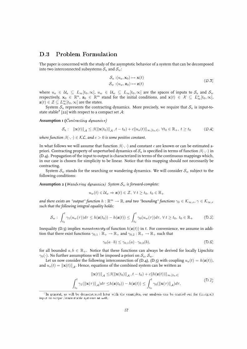
D.3 Problem FormulationThe paper is concerned with the study of the asymptotic behavior of a system that can be decomposedinto two interconnected subsystems Sa and Sw:
Sa :(ua,x0) 7→ x(t)Sw :(uw, z0) 7→ z(t)
(D.3)
where ua ∈ Ua ⊆ L∞[t0,∞], uw ∈ Uw ⊆ L∞[t0,∞] are the spaces of inputs to Sa and Sw
respectively, x0 ∈ Rn, z0 ∈ Rm stand for the initial conditions, and x(t) ∈ X ⊆ Ln∞[t0,∞],
z(t) ∈ Z ⊆ Lm∞[t0,∞] are the states.
System Sa represents the contracting dynamics. More precisely, we require that Sa is input-to-state stable7 [22] with respect to a compact set A:
Assumption 1 (Contracting dynamics)
Sa : ‖x(t)‖A ≤ β(‖x(t0)‖A , t− t0) + c‖ua(t)‖∞,[t0,t], ∀t0 ∈ R+, t ≥ t0 (D.4)
where function β(·, ·) ∈ KL, and c > 0 is some positive constant.
In what follows we will assume that function β(·, ·) and constant c are known or can be estimated a-priori. Contracting property of unperturbed dynamics of Sa is specified in terms of function β(·, ·) in(D.4). Propagation of the input to output is characterized in terms of the continuous mappings which,in our case is chosen for simplicity to be linear. Notice that this mapping should not necessarily becontracting.
System Sw stands for the searching or wandering dynamics. We will consider Sw subject to thefollowing conditions:
Assumption 2 (Wandering dynamics) System Sw is forward-complete:
uw(t) ∈ Uw ⇒ z(t) ∈ Z, ∀ t ≥ t0, t0 ∈ R+
and there exists an "output" function h : Rm → R, and two "bounding" functions γ0 ∈ K∞,e, γ ∈ K∞,e
such that the following integral equality holds:
Sw :∫ t
t0
γ1(uw(τ))dτ ≤ h(z(t0))− h(z(t)) ≤∫ t
t0
γ0(uw(τ))dτ, ∀ t ≥ t0, t0 ∈ R+ (D.5)
Inequality (D.5) implies monotonicity of function h(z(t)) in t. For convenience, we assume in addi-tion that there exist functions γ0,1 : R+ → R+ and γ0,2 : R+ → R+ such that
γ0(a · b) ≤ γ0,1(a) · γ0,2(b), (D.6)
for all bounded a, b ∈ R+. Notice that these functions can always be derived for locally Lipschitzγ0(·). No further assumptions will be imposed a-priori on Sa, Sw.
Let us now consider the following interconnection of (D.4), (D.5) with coupling ua(t) = h(z(t)),and us(t) = ‖x(t)‖A. Hence, equations of the combined system can be written as
‖x(t)‖A ≤β(‖x(t0)‖A , t− t0) + c‖h(z(t))‖∞,[t0,t]∫ t
t0
γ1(‖x(τ)‖A)dτ ≤h(z(t0))− h(z(t)) ≤∫ t
t0
γ0(‖x(τ)‖A)dτ,(D.7)
7In general, as will be demonstrated later with the examples, our analysis can be carried out for (integral)input-to-output/state stable systems as well.
57
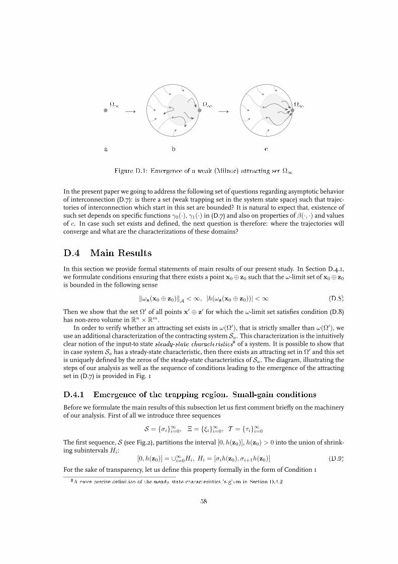
Figure D.1: Emergence of a weak (Milnor) attracting set Ω∞
In the present paper we going to address the following set of questions regarding asymptotic behaviorof interconnection (D.7): is there a set (weak trapping set in the system state space) such that trajec-tories of interconnection which start in this set are bounded? It is natural to expect that, existence ofsuch set depends on specific functions γ0(·), γ1(·) in (D.7) and also on properties of β(·, ·) and valuesof c. In case such set exists and defined, the next question is therefore: where the trajectories willconverge and what are the characterizations of these domains?
D.4 Main ResultsIn this section we provide formal statements of main results of our present study. In Section D.4.1,we formulate conditions ensuring that there exists a point x0⊕ z0 such that the ω-limit set of x0⊕ z0
is bounded in the following sense
‖ωx(x0 ⊕ z0)‖A < ∞, |h(ωz(x0 ⊕ z0))| < ∞ (D.8)
Then we show that the set Ω′ of all points x′ ⊕ z′ for which the ω-limit set satisfies condition (D.8)has non-zero volume in Rn × Rm.
In order to verify whether an attracting set exists in ω(Ω′), that is strictly smaller than ω(Ω′), weuse an additional characterization of the contracting system Sa. This characterization is the intuitivelyclear notion of the input-to state steady-state characteristics8 of a system. It is possible to show thatin case system Sa has a steady-state characteristic, then there exists an attracting set in Ω′ and this setis uniquely defined by the zeros of the steady-state characteristics of Sa. The diagram, illustrating thesteps of our analysis as well as the sequence of conditions leading to the emergence of the attractingset in (D.7) is provided in Fig. 1
D.4.1 Emergence of the trapping region. Small-gain conditionsBefore we formulate the main results of this subsection let us first comment briefly on the machineryof our analysis. First of all we introduce three sequences
S = σi∞i=0, Ξ = ξi∞i=0, T = τi∞i=0
The first sequence, S (see Fig.2), partitions the interval [0, h(z0)], h(z0) > 0 into the union of shrink-ing subintervals Hi:
[0, h(z0)] = ∪∞i=0Hi, Hi = [σih(z0), σi+1h(z0)] (D.9)For the sake of transparency, let us define this property formally in the form of Condition 1
8A more precise denition of the steady-state characteristics is given in Section D.4.2
58
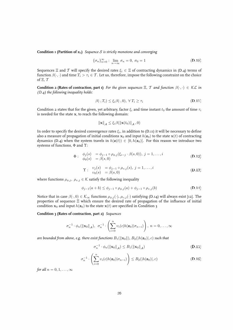
Condition 1 (Partition of z0) Sequence S is strictly monotone and converging
σn∞n=0 : limn→∞
σn = 0, σ0 = 1 (D.10)
Sequences Ξ and T will specify the desired rates ξi ∈ Ξ of contracting dynamics in (D.4) terms offunction β(·, ·) and time Ti > τi ∈ T . Let us, therefore, impose the following constraint on the choiceof Ξ, TCondition 2 (Rates of contraction, part 1) For the given sequences Ξ, T and function β(·, ·) ∈ KL in(D.4) the following inequality holds:
β(·, Ti) ≤ ξiβ(·, 0), ∀ Ti ≥ τi (D.11)
Condition 2 states that for the given, yet arbitrary, factor ξi and time instant t0 the amount of time τi
is needed for the state x, to reach the following domain:
‖x‖A ≤ ξiβ(‖x(t0)‖A , 0)
In order to specify the desired convergence rates ξi, in addition to (D.11) it will be necessary to definealso a measure of propagation of initial conditions x0 and input h(z0) to the state x(t) of contractingdynamics (D.4) when the system travels in h(z(t)) ∈ [0, h(z0)]. For this reason we introduce twosystems of functions, Φ and Υ:
Φ :φj(s) = φj−1 ρφ,j(ξi−j · β(s, 0)), j = 1, . . . , iφ0(s) = β(s, 0) (D.12)
Υ :υj(s) = φj−1 ρυ,j(s), j = 1, . . . , iυ0(s) = β(s, 0) (D.13)
where functions ρφ,j , ρυ,j ∈ K satisfy the following inequality
φj−1(a + b) ≤ φj−1 ρφ,j(a) + φj−1 ρυ,j(b) (D.14)
Notice that in case β(·, 0) ∈ K∞ functions ρφ,j(·), ρυ,j(·) satisfying (D.14) will always exist [12]. Theproperties of sequence Ξ which ensure the desired rate of propagation of the influence of initialcondition x0 and input h(z0) to the state x(t) are specified in Condition 3
Condition 3 (Rates of contraction, part 2) Sequences
σ−1n · φn(‖x0‖A), σ−1
n ·(
n∑
i=0
υi(c|h(z0)|σn−i)
), n = 0, . . . ,∞
are bounded from above, e.g. there exist functions B1(‖x0‖), B2(|h(z0)|, c) such that
σ−1n · φn(‖x0‖A) ≤ B1(‖x0‖A) (D.15)
σ−1n ·
(n∑
i=0
υi(c|h(z0)|σn−i)
)≤ B2(|h(z0)|, c) (D.16)
for all n = 0, 1, . . . ,∞
59
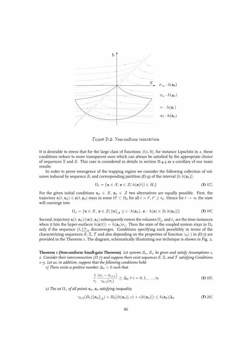
Figure D.2: Non-uniform contraction
It is desirable to stress that for the large class of functions β(s, 0), for instance Lipschitz in s, theseconditions reduce to more transparent ones which can always be satisfied by the appropriate choiceof sequences Ξ and S . This case is considered in details in section D.4.3 as a corollary of our mainresults
In order to prove emergence of the trapping region we consider the following collection of vol-umes induced by sequence Si and corresponding partition (D.9) of the interval [0, h(z0)]:
Ωi = x ∈ X , z ∈ Z| h(z(t)) ∈ Hi (D.17)
For the given initial conditions x0 ∈ X , z0 ∈ Z two alternatives are equally possible. First, thetrajectory x(t,x0) ⊕ z(t, z0) stays in some Ω′ ⊂ Ω0 for all t > t′, t′ ≥ t0. Hence for t → ∞ the statewill converge into
Ωa = x ∈ X , z ∈ Z| ‖x‖A ≤ c · h(z0), z : h(z) ∈ [0, h(z0)] (D.18)
Second, trajectory x(t,x0)⊕z(t, z0) subsequently enters the volumes Ωj , and tj are the time instanceswhen it hits the hyper-surfaces h(z(t)) = h(z0)σj . Then the state of the coupled system stays in Ω0
only if the sequence ti∞i=0 disconverges. Conditions specifying such possibility in terms of thecharacterizing sequences S , Ξ, T and also depending on the properties of function γ0(·) in (D.7) areprovided in the Theorem 1. The diagram, schematically illustrating our technique is shown in Fig. 2.
Theorem 1 (Non-uniform Small-gain Theorem) Let systems Sa, Sw be given and satisfy Assumptions 1,2. Consider their interconnection (D.7) and suppose there exist sequences S , Ξ, and T satisfying Conditions1–3. Let us, in addition, suppose that the following conditions hold:
1) There exists a positive number ∆0 > 0 such that
1τi
(σi − σi+1)γ0,1(σi)
≥ ∆0 ∀ i = 0, 1, . . . ,∞ (D.19)
2) The set Ωγ of all points x0, z0 satisfying inequality
γ0,2(B1(‖x0‖A) + B2(|h(z0)|, c) + c|h(z0)|) ≤ h(z0)∆0 (D.20)
60
is not empty.3) Partial sums of elements from T diverge:
∞∑
i=0
τi = ∞ (D.21)
Then for all x0, z0 ∈ Ωγ state x(t, z0)⊕ z(t, z0) of system (D.7) converges into the set specified by (D.18)
Ωa = x ∈ X , z ∈ Z| ‖x‖A ≤ c · h(z0), z : h(z) ∈ [0, h(z0)]
Proof of the theorem is provided in Appendix 1.The major difference between conditions of Theorem 1 and conventional small-gain theorems
[30],[12] is that the latter involve only input-output or input-state mappings (mappings γ0(·) and con-stant c in our case). This is because interconnected systems are assumed to be input-to-state stableand their internal dynamics, therefore, can be neglected. In our case, however, this is no longer true asdynamics of Sw is generally unstable in the Lyapunov sense. Hence, in order to ensure boundednessof x(t,x0) and h(z(t, z0)), the rate/degree of stability of Sa should be taken into account. Roughlyspeaking, system Sa should ensure a sufficiently high degree of contraction in x0 while input-outputresponse of Sw should be sufficiently small. The rate of contraction in x0 of Sa, according to (D.4), isspecified in terms of the function β(·, ·). Properties of this function that are relevant for convergenceare explicitly accounted for in Condition 3 and (D.21). The domain of admissible initial conditions andactually the small-gain condition (input-state-output properties of Sw and Sa) are defined by (D.19),(D.20) respectively. Notice also that Ωγ is not necessarily a neighborhood of Ωa, thus the convergenceensured by Theorem 1 may not be uniform in x0, z0.
D.4.2 Characterization of the attracting setSmall-gain conditions, even in case of interconnection of Lyapunov-stable systems are usually effec-tive for establishing boundedness of state or outputs. Yet, it is still possible to derive the estimates(like, for instance, (D.18)) of the domains to which the state will converge. These estimates, how-ever, are often too conservative. If a more precise characterization of the domains to which the statewill converge is required additional information on the dynamics of systems Sa and Sw is needed.The question, therefore, is how detailed this information should be? It appears that some additionalknowledge of the steady-state characteristics of system Sa is sufficient to improve the estimates (D.18)substantially.
Let us formally introduce the notion of steady-state characteristic as follows:
Definition 5 We say that system (D.4) has steady-state characteristic χ : R→ R+ with respect to the norm‖x‖A if and only if for each constant ua the following holds:
∀ ua(t) ∈ Ua : limt→∞
ua(t) = ua ⇒ limt→∞
‖x(t)‖A ∈ χ(ua) (D.22)
The key property captured by Definition 5 is that there exists a limit of ‖x(t)‖A as t → ∞ providedthat the limit for ua(t), t →∞ is defined and constant. Notice that the graph of mapping χ should notnecessarily be functional. Therefore, our definition shall allow a fairly large amount of uncertaintyfor Sa. It will be of essential importance, however, that such characterization exists for system Sa.
Not every system, however, obeys the steady-state characteristic χ(·) of Definition 5. There arerelatively simple systems whose state does not converge even in the "norm" sense for constant (con-verging to) inputs as is required in (D.22). In mechanics, physics and biology such systems present alarge class of nonlinear oscillators which can be excited by constant inputs. In order to take such sys-tems into consideration, we introduce a weaker notion, that is steady-state characteristic on average:
61
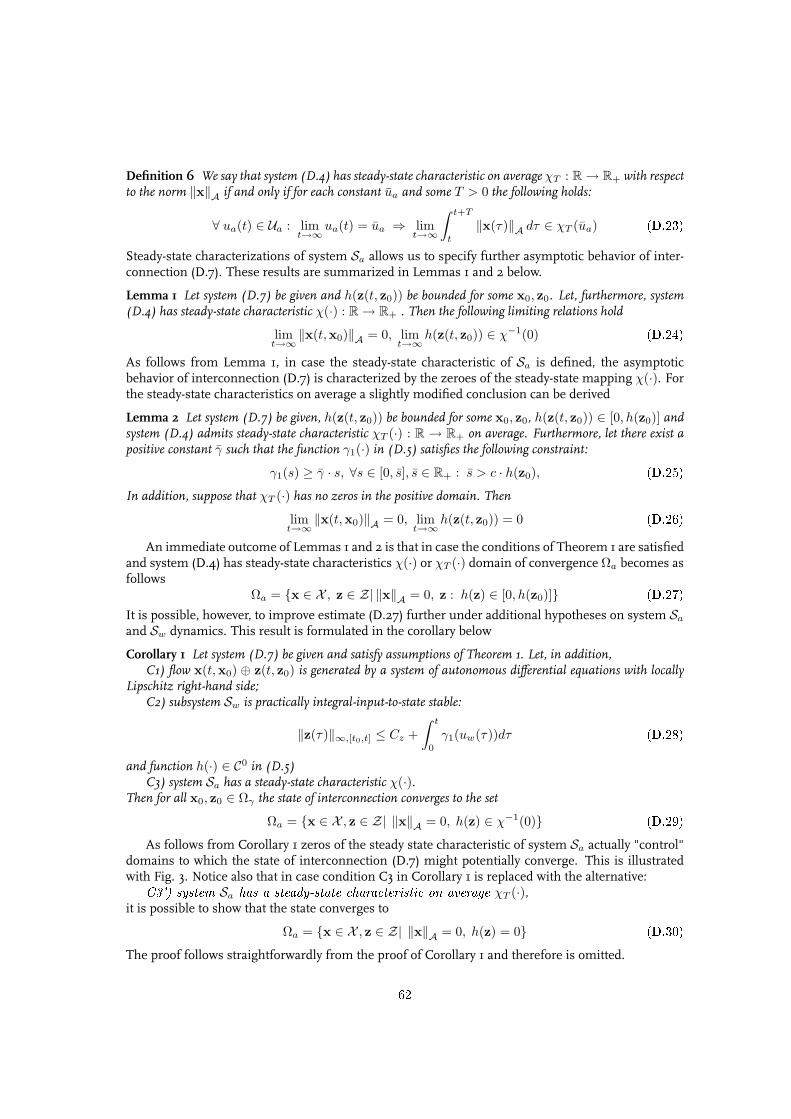
Definition 6 We say that system (D.4) has steady-state characteristic on average χT : R→ R+ with respectto the norm ‖x‖A if and only if for each constant ua and some T > 0 the following holds:
∀ ua(t) ∈ Ua : limt→∞
ua(t) = ua ⇒ limt→∞
∫ t+T
t
‖x(τ)‖A dτ ∈ χT (ua) (D.23)
Steady-state characterizations of system Sa allows us to specify further asymptotic behavior of inter-connection (D.7). These results are summarized in Lemmas 1 and 2 below.
Lemma 1 Let system (D.7) be given and h(z(t, z0)) be bounded for some x0, z0. Let, furthermore, system(D.4) has steady-state characteristic χ(·) : R→ R+ . Then the following limiting relations hold
limt→∞
‖x(t,x0)‖A = 0, limt→∞
h(z(t, z0)) ∈ χ−1(0) (D.24)
As follows from Lemma 1, in case the steady-state characteristic of Sa is defined, the asymptoticbehavior of interconnection (D.7) is characterized by the zeroes of the steady-state mapping χ(·). Forthe steady-state characteristics on average a slightly modified conclusion can be derived
Lemma 2 Let system (D.7) be given, h(z(t, z0)) be bounded for some x0, z0, h(z(t, z0)) ∈ [0, h(z0)] andsystem (D.4) admits steady-state characteristic χT (·) : R → R+ on average. Furthermore, let there exist apositive constant γ such that the function γ1(·) in (D.5) satisfies the following constraint:
γ1(s) ≥ γ · s, ∀s ∈ [0, s], s ∈ R+ : s > c · h(z0), (D.25)In addition, suppose that χT (·) has no zeros in the positive domain. Then
limt→∞
‖x(t,x0)‖A = 0, limt→∞
h(z(t, z0)) = 0 (D.26)
An immediate outcome of Lemmas 1 and 2 is that in case the conditions of Theorem 1 are satisfiedand system (D.4) has steady-state characteristics χ(·) or χT (·) domain of convergence Ωa becomes asfollows
Ωa = x ∈ X , z ∈ Z| ‖x‖A = 0, z : h(z) ∈ [0, h(z0)] (D.27)It is possible, however, to improve estimate (D.27) further under additional hypotheses on system Sa
and Sw dynamics. This result is formulated in the corollary below
Corollary 1 Let system (D.7) be given and satisfy assumptions of Theorem 1. Let, in addition,C1) flow x(t,x0) ⊕ z(t, z0) is generated by a system of autonomous differential equations with locally
Lipschitz right-hand side;C2) subsystem Sw is practically integral-input-to-state stable:
‖z(τ)‖∞,[t0,t] ≤ Cz +∫ t
0
γ1(uw(τ))dτ (D.28)
and function h(·) ∈ C0 in (D.5)C3) system Sa has a steady-state characteristic χ(·).
Then for all x0, z0 ∈ Ωγ the state of interconnection converges to the set
Ωa = x ∈ X , z ∈ Z| ‖x‖A = 0, h(z) ∈ χ−1(0) (D.29)As follows from Corollary 1 zeros of the steady state characteristic of system Sa actually "control"
domains to which the state of interconnection (D.7) might potentially converge. This is illustratedwith Fig. 3. Notice also that in case condition C3 in Corollary 1 is replaced with the alternative:
C3') system Sa has a steady-state characteristic on average χT (·),it is possible to show that the state converges to
Ωa = x ∈ X , z ∈ Z| ‖x‖A = 0, h(z) = 0 (D.30)The proof follows straightforwardly from the proof of Corollary 1 and therefore is omitted.
62
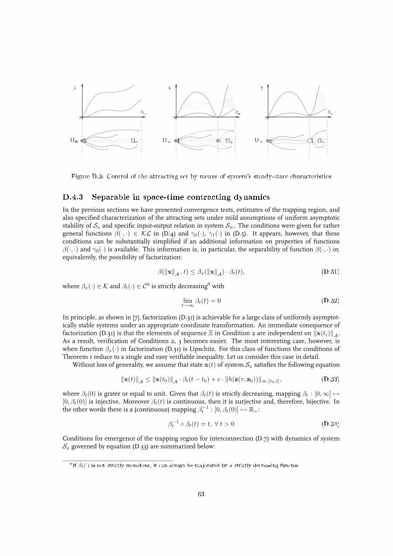
Figure D.3: Control of the attracting set by means of system's steady-state characteristics
D.4.3 Separable in space-time contracting dynamicsIn the previous sections we have presented convergence tests, estimates of the trapping region, andalso specified characterization of the attracting sets under mild assumptions of uniform asymptoticstability of Sa and specific input-output relation in system Sw. The conditions were given for rathergeneral functions β(·, ·) ∈ KL in (D.4) and γ0(·), γ1(·) in (D.5). It appears, however, that theseconditions can be substantially simplified if an additional information on properties of functionsβ(·, ·) and γ0(·) is available. This information is, in particular, the separability of function β(·, ·) or,equivalently, the possibility of factorization:
β(‖x‖A , t) ≤ βx(‖x‖A) · βt(t), (D.31)
where βx(·) ∈ K and βt(·) ∈ C0 is strictly decreasing9 with
limt→∞
βt(t) = 0 (D.32)
In principle, as shown in [7], factorization (D.31) is achievable for a large class of uniformly asymptot-ically stable systems under an appropriate coordinate transformation. An immediate conequence offactorization (D.31) is that the elements of sequence Ξ in Condition 2 are independent on ‖x(ti)‖A.As a result, verification of Conditions 2, 3 becomes easier. The most interesting case, however, iswhen function βx(·) in factorization (D.31) is Lipschitz. For this class of functions the conditions ofTheorem 1 reduce to a single and easy verifiable inequality. Let us consider this case in detail.
Without loss of generality, we assume that state x(t) of system Sa satisfies the following equation
‖x(t)‖A ≤ ‖x(t0)‖A · βt(t− t0) + c · ‖h(z(τ, z0))‖∞,[t0,t], (D.33)
where βt(0) is grater or equal to unit. Given that βt(t) is strictly decreasing, mapping βt : [0,∞] 7→[0, βt(0)] is injective. Moreover βt(t) is continuous, then it is surjective and, therefore, bijective. Inthe other words there is a (continuous) mapping β−1
t : [0, βt(0)] 7→ R+:
β−1t βt(t) = t, ∀ t > 0 (D.34)
Conditions for emergence of the trapping region for interconnection (D.7) with dynamics of systemSa governed by equation (D.33) are summarized below:
9If βt(·) is not strictly monotone, it can always be majorated by a strictly decreasing functon
63
Corollary 2 Let interconnection (D.7) be given, system Sa satisfy (D.33) and function γ0(·) in (D.5) beLipschitz:
|γ0(s)| ≤ Dγ,0 · |s| (D.35)and domain
Ωγ : Dγ,0 ≤(
β−1t
(d
κ · βt(0)
))−1κ− 1
κ
h(z0)
βt(0) ‖x0‖A + βt(0) · c · |h(z0)|(1 + κ
1−d
)+ c|h(z0)|
(D.36)is not empty for some d < 1, κ > 1. Then for all initial conditions x0 z0 ∈ Ωγ state x(t,x0) ⊕ z(t, z0) ofinterconnection (D.7) converges into the set Ωa specified by (D.18). If, in addition, conditions C1)–C3) ofCorollary 1 hold then the domain of convergence is given by (D.27).
A practically important consequence of this corollary concerns systems Sa which are exponentiallystable:
‖x(t)‖A ≤ ‖x(t0)‖ADβ exp(−λt) + c · ‖h(z(t, z0))‖∞,[t0,t], λ > 0, Dβ ≥ 1 (D.37)
For this case domain (D.36) of initial conditions ensuring convergence into Ωa is defined as
Dγ,0 ≤ maxκ>1, d∈(0,1)
−λ
(ln
d
κDβ
)−1κ− 1
κ
h(z0)
Dβ ‖x0‖A + Dβ · c · |h(z0)|(1 + κ
1−d
)+ c|h(z0)|
In the next section we show how this result can be applied to address the problem of outputnonlinear identification for systems which cannot be transformed into the canonic observer formor/and with nonlinear parametrization.
D.5 DiscussionIn the literature of adaptive control, observation and identification a few classes of systems are re-ferred as canonic forms for their ability to poses solutions to the problem and, at the same time,applicability to large variety of relevant physical phenomena. Among these, perhaps, the most widelyknown is the adaptive observer canonical form [2]. Necessary and sufficient conditions for trans-formation of the original system into the observer canonical form can be found, for example, in[16]. These conditions, however, include restrictive requirements of linearization of uncertainty-independent dynamics by output injection, and also they require linear parametrization of the un-certainty. Alternative approaches [3] heavily rely on knowledge of the proper Lyapunov function foruncertainty-independent part and still assume linear parametrization.
Let us now demonstrate how these restrictions can be lifted by application our result to the prob-lem of state and parameter observation. Let us consider classes of systems which can be transformedby means of the feedback, static or dynamic10, into the following form:
x = f0(x, t) + f(ξ(t), θ)− f(ξ(t), θ) + ε(t), (D.38)
whereε(t) ∈ Lm
∞[t0,∞], ‖ε(τ)‖∞,[t0,t] ≤ ∆ε
is external perturbation with known ∆ε, and x ∈ Rn. Function ξ : R+ → Rξ is a function oftime, which possibly includes available measurements of the state, and θ, θ ∈ Ωθ ⊂ Rd are the
10Notice that conventional observers in control theory could be viewed as dynamic feedbacks of the specic class
64
unknown and estimated parameters of function f(·) respectively and set Ωθ is bounded. We assumethat function f(ξ(t),θ) is locally bounded in θ uniformly in ξ:
‖f(ξ(t), θ)− f(ξ(t), θ)‖ ≤ Df‖θ − θ‖+ ∆f
and the values of Df ∈ R+, ∆f are available. Function f0(·) in (D.38) is assumed to satisfy thefollowing condition:
Assumption 3 Systemx = f0(x, t) + u(t) (D.39)
is forward-complete. Furthermore, for all u(t) such that
‖u(t)‖∞,[t0,t] ≤ ∆u + ‖u0(τ)‖∞,[t0,t], ∆u ∈ R+
there exist bounded set A, c > 0 and function ∆ : R+ → R+ satisfying the following inequality:
‖x(t)‖A∆(∆u)≤ β(t− t0) ‖x(t0)‖A∆(∆u)
+ c‖u0(τ)‖∞,[t0,t]
where β(·) : R+ → R+, limt→∞ β(t) = 0 is strictly decreasing function.
Let us consider the following auxiliary system
λ = S(λ), λ(t0) = λ0 ∈ Ωλ ⊂ Rλ (D.40)
where Ωλ ⊂ Rn is bounded and S(λ) is locally Lipschitz. Further, suppose that the following as-sumption holds for system (D.40)
Assumption 4 System (D.40) is Poisson stable in Ωλ that is
∀ λ′ ∈ Ωλ, t′ ∈ R+ ⇒ ∃t′′ > t : ‖λ(t′′, λ′)− λ′‖ ≤ ε,
where ε is arbitrary small positive constant. Moreover, trajectory λ(t,λ0) is dense in Ωλ:
∀λ′ ∈ Ωλ, ε ∈ R>0 ⇒ ∃ t ∈ R+ : ‖λ′ − λ(t, λ0)‖ < ε
Now we are ready to formulate the following statement:
Corollary 3 Let us consider system (D.38) and suppose that the following conditions holdC4) vector-field f0(x, t) in (D.38) satisfies Assumption 3;C5) there exists and known system (D.40) satisfying Assumption 4;C6) there exists locally Lipschitz η : Rλ → Rd:
‖η(λ′)− η(λ′′)‖ ≤ Dη‖λ′ − λ′′‖such that set η(Ωλ) is dense in Ωθ;
C7) system (D.38) has steady-state characteristic with respect to the norm
‖·‖A∆(M), M = 2∆f + ∆ε + δ
and input θ, where δ is some positive (arbitrary small) constant.Consider the following interconnection of (D.38), (D.40):
x = f0(x, t) + f(ξ(t), θ)− f(ξ(t), θ) + ε(t)
θ = η(λ)
λ = γ ‖x(t)‖A∆(M)S(λ),
(D.41)
65
where γ > 0 satisfies the following inequality
γ ≤(
β−1t
(d
κ · βt(0)
))−1κ− 1
κ
1
Dλ
(βt(0)
(1 + κ
1−d
)+ 1
)
Dλ = c ·Df ·Dη · maxλ∈Ωλ
‖S(λ)‖(D.42)
for some d ∈ (0, 1), κ ∈ (1,∞). Then, for λ(t0) = λ0, some θ′ ∈ Ωθ and all x(t0) = x0 ∈ Rn thefollowing holds:
limt→∞
‖x(t)‖A∆(M)= 0, lim
t→∞θ(t) = θ′ ∈ Ωθ (D.43)
Notice that again, as has been pointed out in the previous section, in case the dynamics of (D.39) isexponentially stable with the rate of convergence equal to ρ and β(0) = Dβ , condition (D.42) willhave the following form:
γ ≤ −ρ
(ln
d
κDβ
)−1κ− 1
κ
1
Dλ
(Dβ
(1 + κ
1−d
)+ 1
)
According to Corollary 3, for rather general class of systems (D.38) it is possible to design estimatorθ(t) which guarantees that not only ”error” vector x(t) reaches a neighborhood of the origin, but alsothat the estimates θ(t) converge to some θ′ in Ωθ. Both these facts together with additional nonlinearpersistent excitation conditions [5],[24]
∃T > 0, ρ ∈ K : ∀ T = [t, t + T ], t ∈ R+ ⇒ ∃τ ∈ T : |f(ξ(τ),θ)− f(ξ(τ), θ′)| ≥ ρ(‖θ − θ′‖)
in principle allow to estimate domains of convergence for θ(t).Concluding this section we would like to mention that statements of Theorem 1 and Corollaries
1–3 constitute additional theoretical tools for analysis of asymptotic behavior of integral input-to-statesystems. In particular they are complementary to the results of [1] where asymptotic stability of thefollowing type of systems
x = f(x),z = q(x, z), f : Rn → Rn, q : Rn × Rm → Rm
was considered under assumption that the x-subsystem is globally asymptotically stable and the z-subsystem is integral input-to-state stable. In contrast to this our results apply to establishing asymp-totic convergence in the systems of the following structure
x = f(x, z),z = q(x, z), f : Rn × Rm → Rn
where the x-subsystem is input-to-state stable, and z-subsystem could be practically integral input-to-state stable (see Corollary 1), although in general no stability assumptions are imposed on it.
D.6 ExamplesIn this section we provide two examples illustrating proposed techniques in application to the prob-lem of parameter identification of nonlinear parameterized systems and those which cannot be trans-formed into the canonical adaptive observer form.
66
The first example is merely academical illustration to Corollary 3, where only one parameter isunknown and the system itself is the first-order differential equation. The second example illustratespossible application of our results to the problems of identification of dynamics in the living cells.
Example 1. Let us consider the following system
x = −kx + sin(xθ + θ) + u, k > 0, θ ∈ [−a, a] (D.44)
where θ is the unknown parameter, and u is the control input. Without loss of the generality we leta = 1, k = 1. The problem is to estimate parameter θ from the measurements of x and also tosteer the system to the origin. Clearly, choice u = − sin(xθ + θ) transforms (D.44) into the followingequation
x = −kx + sin(xθ + θ)− sin(xθ + θ) (D.45)which satisfies Assumption 3. Moreover, system
λ1 = λ1
λ2 = −λ2, λ21(t0) + λ2
2(t0) = 1
with mapping η = (1, 0)T λ satisfy Assumption 4 and therefore
λ1 = γ|x|λ1
λ2 = −γ|x|λ2, λ21(t0) + λ2
2(t0) = 1(D.46)
would be a candidate for the control and parameter estimation algorithm. According to Corollary 3,the goal will be reached if parameter γ in (D.46) obeys the following constraint
γ ≤ −ρ
(ln
d
κDβ
)−1κ− 1
κ
1
Dλ
(Dβ
(1 + κ
1−d
)+ 1
) , ρ = k = 1, Dβ = 1, Dλ = 1
for some d ∈ (0, 1), κ ∈ (1,∞). Hence, choosing, for example, d = 0.5, κ = 2 we obtain that choice
0 < γ < − ln(
0.52
)12· 16
= 0.1155
suffices to ensure thatlim
t→∞x(t) = 0, lim
t→∞θ(t) = θ
We simulated system (D.45), (D.46) with θ = 0.3, γ = 0.1 and initial conditions x(t0) randomlydistributed in the interval [−1, 1]. Results of the simulation are illustrated with Figure 4, where thephase plots of system (D.45), (D.46) as well as the trajectories of θ(t) are provided.
Example 2. Let us consider the problem modelling electrical activity in the biological cells fromthe input-output data in the current clamp experiments. The simplest mathematical model, whichcaptures fairly large variety of phenomena like periodic bursting in response to constant stimulationis the classical Hindmarsh and Rose model without adaptation currents [9]:
x1 = −ax31 + bx2
1 + x2 + αu
x2 = c− βx2 − dx21
(D.47)
where variable x1 is the membrane potential, x2 stands for the ionic currents in the cell, u is theinput current, and a, b, c, d, α, β ∈ R are parameters. While parameters of the first equation can, inprinciple, be identified experimentally by blocking the ionic channels in the cells and measuring the
67
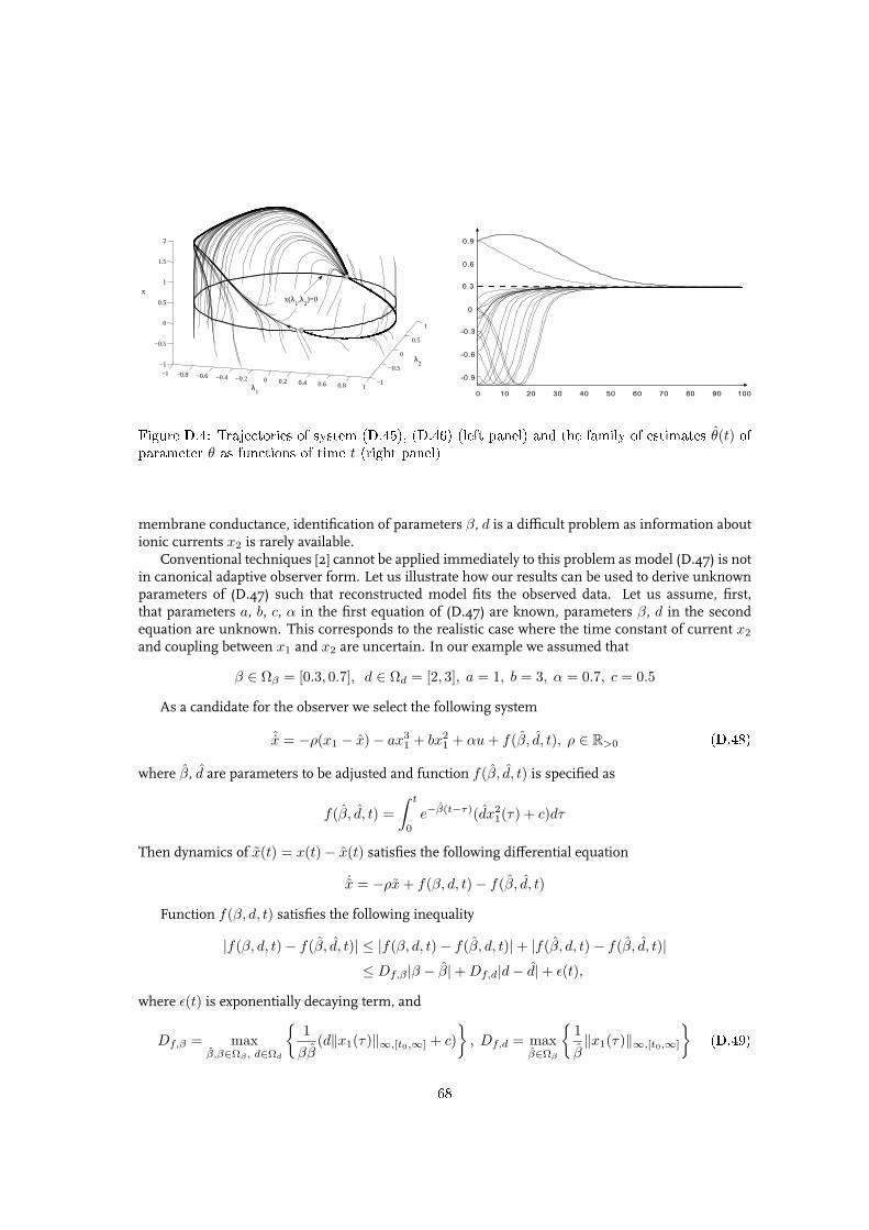
−1 −0.8 −0.6 −0.4 −0.2 0 0.2 0.4 0.6 0.8 1−1
−0.5
0
0.5
1
−1
−0.5
0
0.5
1
1.5
2
x
λ1
λ2
x(λ1,λ
2)=0
0 10 20 30 40 50 60 70 80 90 100
-0.9
-0.6
-0.3
0
0.3
0.6
0.9
Figure D.4: Trajectories of system (D.45), (D.46) (left panel) and the family of estimates θ(t) ofparameter θ as functions of time t (right panel)
membrane conductance, identification of parameters β, d is a difficult problem as information aboutionic currents x2 is rarely available.
Conventional techniques [2] cannot be applied immediately to this problem as model (D.47) is notin canonical adaptive observer form. Let us illustrate how our results can be used to derive unknownparameters of (D.47) such that reconstructed model fits the observed data. Let us assume, first,that parameters a, b, c, α in the first equation of (D.47) are known, parameters β, d in the secondequation are unknown. This corresponds to the realistic case where the time constant of current x2
and coupling between x1 and x2 are uncertain. In our example we assumed that
β ∈ Ωβ = [0.3, 0.7], d ∈ Ωd = [2, 3], a = 1, b = 3, α = 0.7, c = 0.5
As a candidate for the observer we select the following system
ˆx = −ρ(x1 − x)− ax31 + bx2
1 + αu + f(β, d, t), ρ ∈ R>0 (D.48)
where β, d are parameters to be adjusted and function f(β, d, t) is specified as
f(β, d, t) =∫ t
0
e−β(t−τ)(dx21(τ) + c)dτ
Then dynamics of x(t) = x(t)− x(t) satisfies the following differential equation
˙x = −ρx + f(β, d, t)− f(β, d, t)
Function f(β, d, t) satisfies the following inequality
|f(β, d, t)− f(β, d, t)| ≤ |f(β, d, t)− f(β, d, t)|+ |f(β, d, t)− f(β, d, t)|≤ Df,β |β − β|+ Df,d|d− d|+ ε(t),
where ε(t) is exponentially decaying term, and
Df,β = maxβ,β∈Ωβ , d∈Ωd
1
ββ(d‖x1(τ)‖∞,[t0,∞] + c)
, Df,d = max
β∈Ωβ
1
β‖x1(τ)‖∞,[t0,∞]
(D.49)
68
Furthermore, Assumption 3 is satisfied for system
˙x = −ρx + υ(t), ‖υ(τ)‖∞,[t0,t] ≤ ∆u + ‖υ0(τ)‖∞,[t0,t]
with
∆(∆u) =∆u
ρ, c = 1
Let us define subsystem (D.40). Consider the following system of differential equations
λ1 = λ2
λ2 = −ω21λ1
λ3 = λ4
λ4 = −ω22λ3, λ0 = (1, 0, 1, 0)T
(D.50)
where Ωλ is the ω-limit set of the point λ0, and ω1, ω2 ∈ R. System, therefore, satisfies Assumption4. Given that domains Ωβ , Ωd are known, let us select
η : Rn → R2, η = (η1(λ), η2(λ))
β = η1(λ) =12
(2 arcsin(λ1)
π+ 1
)· 0.4 + 0.3, d = η2(λ) =
12
(2 arcsin(λ3)
π+ 1
)+ 2
(D.51)
Choosingω1
ω2= π
we ensure that η(Ωλ) id dense in Ωβ ×Ωd. Given that β, d are bounded, Df,β and Df,d in (D.49) arealso bounded (for the given range of parameters signal x1(t) is always bounded). Hence, accordingto Corollary 3, interconnection of (D.48), (D.51) and
λ1 = γ‖x(t)‖∆(δ) · λ2
λ2 = −γ‖x(t)‖∆(δ) · ω21λ1
λ3 = γ‖x(t)‖∆(δ) · λ4
λ4 = −γ‖x(t)‖∆(δ) · ω22λ3, λ0 = (1, 0, 1, 0)T
with arbitrary small δ > 0 and properly chosen γ > 0 ensures that
limt→∞
‖x(t)‖∆(δ) = 0, limt→∞
β(t) = β′ ∈ Ωβ , limt→∞
d(t) = d′ ∈ Ωd
This, would in turn imply successful fit of the observations to the model.We simulated the system with ρ = 10 and γ = 3 · 10−4 for β = 0.5, d = 2.5. The results of the
simulations are provided in figures 5 (trajectories x1(t), x(t)) and 6 (estimates β(t) and d(t)). It canbe seen from these figures that reconstruction is successful and parameters converge into a smallneighborhood of the actual values.
D.7 ConclusionWe proposed new tools for analysis of asymptotic behavior for a class of dynamical systems. Inparticular, we considered an interconnection of input-to-state stable system with an unstable or in-tegrally input-to-state dynamics. Our results allow to address a variety of relevant problems when
69

0 0.1 0.2 0.3 0.4 0.5-2
0
2
4
6
8
10
12
14
16
time [s]
x1
model
reconstruction
0 0.1 0.2 0.3 0.4 0.5-2
-1
0
1
2
3
x1
model
reconstruction
0 0.1 0.2 0.3 0.4 0.5-15
-10
-5
0
5
time (s)
x2
Figure D.5: Trajectories x1(t) and x(t) in the beginning of the simulation (left panel), and at theend of the simulation (right panel)
0.35 0.4 0.45 0.5 0.55 0.6 0.65 0.72
2.1
2.2
2.3
2.4
2.5
2.6
2.7
2.8
2.9
3
β
d
Figure D.6: Searching dynamics in the bounded parameter space
70
the convergence might not be unform in initial condition. It is necessary to notice that we do notrequire complete knowledge of the dynamical systems in question. Only qualitative information like,for instance, characterization of input-to-state stability of is necessary for application of our results.We have also demonstrated how our analysis can be used in the problems of synthesis and design.In particular, to the problems of nonlinear regulation and parameter identification of nonlinear pa-rameterized systems. Provided examples show relevance of our approach in those domains whereapplication of the standard techniques is either not possible or complicated.
D.8 AcknowledgmentThe authors are thankful to Peter Jurica and Tatiana Tyukina for their enthusiastic help and commentsduring preparation of this manuscript.
D.9 AppendixProof of Theorem 1. Let conditions of the theorem be satisfied for the given t0 ∈ R+: x(t0) = x0,z(t0) = z0. Notice that in this case h(z0) ≥ 0 overwise requirement (D.20) will be violated. Let usconsider the sequence (D.17) volumes Ωi induced by S :
Ωi = x ∈ X , z ∈ Z| h(z(t)) ∈ HiTo prove the theorem we shall show that 0 ≤ h(z(t)) ≤ h(z0) for all t ≥ t0. For the given partition(D.17) we consider two alternatives.
First, in the degenerative case, the state x(t) ⊕ z(t) enters some Ωj , j ≥ 0 and stays there for allt ≥ t0 which automatically guarantees that 0 ≤ |h(z)| ≤ h(z0). Then, according to (D.4) trajectoryx(t) satisfies the following inequality:
‖x(t)‖A ≤ β(‖x0‖A , t− t0) + c‖h(z(t))‖∞,[t0,t] ≤ β(‖x0‖A , t− t0) + c|h(z0)| (D.52)
Taking into account that β(·, ·) ∈ KL we can conclude that (D.52) implies that
lim supt→∞
‖x(t)‖A = c|h(z0)| (D.53)
Therefore statements of the theorem hold.Let us consider the second alternative, where the state x(t) ⊕ z(t) does not belong to Ωj for all
t ≥ t0. Given that h(z(t)) is monotone and non-increasing in t, this implies that there exists anordered sequence of time instants tj :
t0 > t1 > t2 · · · tj > tj+1 · · · (D.54)
such thath(z(ti)) = σih(z0) (D.55)
Hence in order to prove the theorem we must show that the sequence ti∞i=0 does not converge. Inthe other words, the boundary σ∞h(z0) = 0 will not be reached in finite time.
In order to do this let us estimate the upper bounds for the following differences
Ti = ti+1 − ti
Taking into account inequality (D.5) and the fact that γ0(·) ∈ Ke we can derive that
h(z(ti))− h(z(ti+1)) ≤ Ti maxτ∈[ti,ti+1]
γ0(‖x(τ)‖A) ≤ Tiγ0(‖x(τ)‖A∞,[ti,ti+1]) (D.56)
71

According to the definition of ti in (D.55) and noticing that sequence S is strictly decreasing we have
h(z(ti))− h(z(ti+1)) = (σi − σi+1)h(z0) > 0
Hence h(z0) > 0 implies that γ0(‖x(τ)‖A∞,[ti,ti+1]) > 0 and, therefore, (D.56) results in the follow-
ing estimate of Ti:
Ti ≥ h(z(ti))− h(z(ti+1))γ0(‖x(τ)‖A∞,[ti,ti+1]
)=
h(z0)(σi − σi+1)γ0(‖x(τ)‖A∞,[ti,ti+1]
)(D.57)
Taking into account that h(z(t)) is non-increasing over [ti, ti+1] and using (D.4) we can bound thenorm ‖x(τ)‖A∞,[ti,ti+1]
as follows
‖x(τ)‖A∞,[ti,ti+1]≤ β(‖x(ti)‖A , 0) + c‖h(z(τ))‖∞,[ti,ti+1] ≤ β(‖x(ti)‖A , 0) + c · σih(z0) (D.58)
Hence, combining (D.57) and (D.58) we obtain that
Ti ≥ h(z0)(σi − σi+1)γ0(σi(σ−1
i β(‖x(ti)‖A , 0) + c · h(z0)))
Then, using property (D.6) of function γ0 we can derive that
Ti ≥ h(z0)(σi − σi+1)γ0,1(σi)
1γ0,2(σ−1
i β(‖x(ti)‖A , 0) + c · h(z0)))(D.59)
Taking into account condition (D.21) of the theorem, the theorem will be proven if we assure that
Ti ≥ τi (D.60)
for all i = 0, 1, 2, . . . ,∞. We prove this claim by induction with respect to index i = 0, 1, . . . ,∞. Westart with i = 0, and then show that for all i > 0 the following implication holds
Ti ≥ τi ⇒ Ti+1 ≥ τi+1 (D.61)
Let us prove that (D.60) holds for i = 0. For this purpose consider the following term (σi − σi+1)/γ0,1(σi).As follows immediately from conditions of the theorem, equation (D.19), we have that
σi − σi+1
γ0,1(σi)≥ τi∆0 ∀ i ≥ 0 (D.62)
In particularσ0 − σ1
γ0,1(σ0)≥ τ0∆0
Therefore, inequality (D.59) reduces to
T0 ≥ τ0∆0h(z0)
γ0,2(σ−10 β(‖x(t0)‖A , 0) + c · h(z0))
(D.63)
Moreover, taking into account Condition 3 and (D.12), (D.13) we can derive the following estimate:
σ−10 β(‖x(t0)‖A , 0) ≤ σ−1
0 φ0(‖x(t0)‖A) + σ−10 υ0(c · |h(z0)|σ0) ≤ B1(‖x0‖A) + B2(|h(z0)|, c)
According to the theorem conditions x0 and z0 satisfy inequality (D.20). This in turn implies that
γ0,2(σ−10 β(‖x(t0)‖A , 0)+c·h(z0)) ≤ γ0,2(B1(‖x0‖A)+B2(|h(z0)|, c)+c·h(z0)) ≤ ∆0·h(z0) (D.64)
72
Combining (D.63) and (D.64) we obtain the desired inequality
T0 ≥ τ0∆0h(z0)
γ0,2(σ−10 β(‖x(t0)‖A , 0) + c · h(z0))
≥ τ0∆0h(z0)∆0h(z0)
= τ0
Thus the basis of induction is proven.Let us assume that (D.60) holds for all i = 0, . . . , n, n ≥ 0. We shall prove now that implication
(D.61) holds for i = n. Consider the term β(‖x(tn+1)‖A , 0):
β(‖x(tn+1)‖A , 0) ≤ β(β(‖x(tn)‖A , Tn) + c‖h(z(τ))‖∞,[tn,tn+1], 0)
≤ β(β(‖x(tn)‖A , Tn) + c · σn · h(z0), 0)
Taking into account Condition 2 (specifically, inequality (D.11)) and (D.12)– (D.14) we can derive that
β(‖x(tn+1)‖A , 0) ≤ β(ξn · β(‖x(tn)‖A), 0) + c · σn · h(z0), 0) ≤ φ1(‖x(tn)‖A) + υ1(c · |h(z)0| · σn)(D.65)
Notice that, according to the inductive hypothesis (Ti ≥ τi) the following holds
‖x(ti+1)‖A ≤ β(‖x(ti)‖A , Ti) + c · σi · h(z0) ≤ ξiβ(‖x(ti)‖A , 0) + c · σi · h(z0) (D.66)
for all i = 0, . . . , n. Then (D.65), (D.66), (D.12)– (D.14) imply that
β(‖x(tn+1)‖A , 0) ≤ φ1(ξiβ(‖x(tn−1)‖A , 0) + c · σn−1 · h(z0)) + υ1(c · |h(z)0| · σn)≤ φ2(‖x(tn−1)‖A) + υ2(c · |h(z0)| · σn−1) + υ1(c · |h(z0)| · σn)
≤ φn+1(‖x0‖A) +n+1∑
i=1
υi(c · |h(z0)|σn+1−i) ≤ φn+1(‖x0‖A) +n+1∑
i=0
υi(c · |h(z0)|σn+1−i)
(D.67)
According to Condition 3, term
σ−1n+1
(φn+1(‖x0‖A) +
n+1∑
i=0
υi(c · |h(z0)|σn+1−i)
)
is bounded from above by the sum
B1(‖x0‖A) + B2(|h(z0)|, c)Therefore, monotonicity of γ0,2, estimate (D.67) and inequality (D.20) lead to the following inequality
γ0,2(σ−1n+1β(‖x(tn+1‖A), 0) + c · h(z0)) ≤ γ0,2(B1(‖x0‖A) + B2(|h(z0)|, c) + c · h(z0)) ≤ ∆0
Hence, according to (D.59), (D.62) we have:
Tn+1 ≥ (σn+1 − σn)γ0,1(σn+1)
h(z0)γ0,2(σ−1
n+1β(‖x(tn+1)‖A , 0) + c · h(z0))≥ τn+1
∆0h(z0)∆0h(z0)
= τn+1
Thus implication (D.61) is proven. This implies that h(z(t)) ∈ [0, h(z0)] for all t ≥ t0 and, conse-quently, that (D.53) holds. The theorem is proven.
Proof of Lemma 1. As follows from the lemma assumptions, h(z(t, z0)) is bounded. Let us, forcertainty, it and belongs to the following interval [a, h(z0)], a ≤ h(z0). Therefore, as follows from(D.5) we can conclude that
0 ≤∫ ∞
t0
γ1(‖x(τ,x0)‖A)dτ ≤ h(z0)− h(z(t, z0)) ≤ ∞ (D.68)
73

On the other hand, taking into account that h(z(t, z0)) is bounded and monotone in t (every sub-sequence of which is again monotone) and applying Bolzano-Weierstrass theorem we can concludethat h(z(t, z0)) converges in [a, h(z0)]. In particular, there exists h ∈ [a, h(z0)] such that
limt→∞
h(z(t, z0)) = h (D.69)
According to the lemma assumptions, system Sa has the steady-state characteristics. This means thatthere exists constant x ∈ R+ such that
limt→∞
‖x(t,x0)‖A = x (D.70)
Suppose that x > 0. Then it follows from (D.70) that there exists time instant t1 < ∞ and someconstant 0 < δ < x such that
‖x(t)‖A ≥ δ ∀t ≥ t1
Hence using (D.68) and noticing that γ1 ∈ Ke we obtain
∞ > h(z0)− h(z0) ≥ limT→∞
∫ T
t1
γ1(δ)dτ = ∞
Thus we obtained the contradiction. Hence, x = 0 and, consequently,
limt→∞
‖x(t)‖A = 0
Then, according to the notion of steady-state characteristic in Definition 5 this is only possible ifh ∈ χ−1(0). The lemma is proven.
Proof of Lemma 2. Analogously to the proof of Lemma 1 we notice that (D.68) holds. This,however, implies that for any constant and positive T the following limit
limt→∞
∫ t+T
t
γ1(‖x(τ)‖A)dτ
exists and equals to zero. Furthermore, h(z(t, z0)) ∈ [0, h(z0)] for all t ≥ t0. Hence, there exists timeinstant t′ such that
‖x(t)‖A ≤ c · h(z0) + ε, ∀ t ≥ t′,
where ε > 0 is arbitrary small. Then taking into account (D.25) we can conclude that
limt→∞
∫ t+T
t
γ1(‖x(τ)‖A)dτ ≥ γ
∫ t+T
t
‖x(τ)‖A dτ = 0 (D.71)
Given that (D.69) holds, system (D.4) has steady-state characteristic on average and that χT (·) hasno zeros in the positive domain, limiting relation (D.71) is possible only if h = 0. Then, according to(D.4), limt→∞ ‖x(t)‖A = 0. The lemma is proven.
Proof of Corollary 1. As follows from Theorem 1, state x(t,x0)⊕ z(t, z0) converges to the set Ωa
specified by (D.18). Hence h(z(t, z0)) is bounded. Then, according to (D.5), estimate (D.68) holds.This in combination with condition (D.28) implies that z(t, z0) is bounded. In the over words
x(t,x0)⊕ z(t, z0) ∈ Ω′ ∀ t ≥ t0
where Ω′ is a bounded subset in Rn × Rm. Applying Bolzano-Weierstrass theorem we can concludethat for every point x0 ⊕ z0 ∈ Ωγ there is an ω-limit set ω(x0 ⊕ z0) ⊆ Ω′ (non-empty).
74
As follows from C3) and Lemma 1 the following holds:
limt→∞
h(z(t, z0)) ∈ χ−1(0)
Therefore, given that h(·) ∈ C0 we can obtain that
limti→∞
h(z(ti, z0)) = h( limti→∞
z(ti, z0)) = h(ωz(x0 ⊕ z0)) ∈ χ−1(0)
In the other words:
ωz(x0 ⊕ z0) ⊆ Ωh = x ∈ Rn, z ∈ Rm| h(z) ∈ χ−1(0)Moreover
ωx(x0 ⊕ z0) ⊆ Ωa = x ∈ Rn, z ∈ Rm| ‖x‖A = 0According to assumption C1, flow x(t,x0) ⊕ z(t, z0) is generated by a system of autonomous differ-ential equations with locally Lipschitz right-hand side. Then, as follows from [13] (Lemma 4.1, page127)
limt→∞
dist(x(t,x0)⊕ z(t, z0), ω(x0 ⊕ z0)) = 0
Noticing that
dist(x(t,x0)⊕ z(t, z0), ω(x0 ⊕ z0)) ≥ dist(x(t,x0), Ωa) + dist(z(t, z0), Ωh)
we can finally obtain that
limt→∞
dist(x(t,x0), Ωa) = 0, limt→∞
dist(z(t, z0), Ωh) = 0
The corollary is proven.Proof of Corollary 2. As follows from Theorem 1, the corollary will be proven if Conditions 1
– 3 are satisfied and also (D.19), (D.20), (D.21) hold. In order to satisfy Condition 1 we select thefollowing sequence S:
S = σi∞i=0, σi =1κi
, κ ∈ R+, κ > 1 (D.72)
Let us chose sequences T and Ξ as follows:
T = τi∞i=0, τi = τ∗, (D.73)
Ξ = ξi∞i=0, ξi = ξ∗, (D.74)where τ∗, ξ∗ are positive, yet to be defined, constants. Notice that choosing T as in (D.73) automat-ically fulfills condition (D.21) of Theorem 1. On the other hand, taking into account (D.33) and thatβt(t) is monotonically decreasing in t, this choice defines constant ξ∗ as follows:
βt(τ∗) ≤ ξ∗ < βt(0) (D.75)
Given that inverse β−1t exists (see, (D.34)), this choice is always possible. In particular, (D.75) will be
satisfied for the following values of τ∗:
τ∗ ≥ β−1t (ξ∗) (D.76)
Let us now find the values for τ∗ and ξ∗ such that Condition 3 is also satisfied. For this reasonconsider systems of functions Φ, Υ specified by equations (D.12), (D.13). Notice that function β(s, 0)in (D.12), (D.13) is linear for system (D.33)
β(s, 0) = s · βt(0),
75
and therefore functions ρφ,j(·), ρυ,j are the identity maps. Hence, Φ, Υ reduce to the following
Φ :φj(s) = φj−1 · ξ∗ · β(s, 0) = ξ∗ · βt(0) · φj−1(s), j = 1, . . . , iφ0(s) = βt(0) · s (D.77)
Υ :υj(s) = φj−1(s), j = 1, . . . , iυ0(s) = βt(0) · s (D.78)
Taking into account (D.72), (D.77), (D.78) let us explicitly formulate requirements (D.15), (D.16) inCondition 3. These conditions are equivalent to boundedness of the following functions
‖x(t0)‖A · βt(0) · κn(ξ∗ · βt(0))n (D.79)
κn
(βt(0)
c|h(z0)|κn
+βt(0)c|h(z0)|
κn−1+ βt(0)
n∑
i=2
c|h(z0)| 1kn−i
(ξ∗ · βt(0))i−1
)
= βt(0)c|h(z0)|+ βt(0)c|h(z0)|κ(
1 +n∑
i=2
κi−1(ξ∗ · βt(0))i−1
) (D.80)
Boundedness functions B1(‖x0‖A) and B2(|h(z0)|, c) is ensured if ξ∗ satisfy the following inequality
ξ∗ ≤ d
κ · βt(0)(D.81)
for some 0 ≤ d < 1. Notice that κ > 1, βt(0) ≥ 1 imply that ξ∗ ≤ 1 and therefore constant τ∗
satisfying (D.76) will always be defied. Hence, according to (D.79), (D.80), functions B1(‖x0‖A) andB2(|h(z0)|, c) satisfying Condition 3 can be chosen as
B1(‖x0‖A) = βt(0) ‖x0‖A ; B2(|h(z0)|, c) = βt(0) · c · |h(z0)|(
1 +κ
1− d
)(D.82)
In order to apply Theorem 1 we have to check the remaining conditions (D.19) and (D.20). Thiswill involve availability of factorization (D.6) for the function γ0(·). According to assumption (D.35)of the corollary function γ0(·) is Lipschitz:
|γ0(s)| ≤ Dγ,0 · |s|This allows us to choose function γ0,1(·) and γ0,2(·) as follows:
γ0,1(s) = s, γ0,2(s) = Dγ,0 · s (D.83)
Condition (D.19), therefore, is equivalent to solvability of the following inequality:(
1κi− 1
κi+1
)κi
τ∗≥ ∆0 (D.84)
Taking into account inequalities (D.76), (D.81) we can derive that solvability of
∆0 =(
β−1t
(d
κ · βt(0)
))−1κ− 1
κ(D.85)
implies existence of ∆0 > 0 satisfying (D.84) and, consequently, condition (D.19) of Theorem 1.Given that d < 1, κ > 1 and βt(0) ≥ 1 positive solution to (D.85) is always defined. Hence, the proofwill be complete and the claim is non-vacuous if domain
Dγ,0 ≤(
β−1t
(d
κ · βt(0)
))−1κ− 1
κ
h(z0)
βt(0) ‖x0‖A + βt(0) · c · |h(z0)|(1 + κ
1−d
)+ c|h(z0)|
76
is not empty. The corollary is proven.Proof of Corollary 3. Let λ(τ, λ0) be a solution of system (D.40). Consider it as a function of
variable τ . Let us pick some monotone, strictly increasing function σ such that the following holds
τ = σ(t), σ : R+ → R+
Given that η(Ωλ) is dense in Ωθ, for any θ ∈ Ωθ there always exists vector λθ ∈ Ωλ such thatη(λθ) = θ + εθ, where ‖εθ‖ is arbitrary small. Furthermore, λ(τ) is dense in Ωλ, hence there is apoint λ∗ = λ(τ∗,λ0), which is arbitrary close to λθ. Consider the following difference
f(ξ(t), θ)− f(ξ(t), θ) = f(ξ(t),θ)− f(ξ(t), η(λ∗)) + f(ξ,η(λ∗))− f(ξ, η(λ(σ(t))))
Function f(·) is locally bounded and η(·) is Lipschitz, then
‖f(ξ, θ)− f(ξ, η(λ∗))‖ ≤ Df‖εθ‖+ ∆f = ∆θ + ∆f
where ∆θ is arbitrary small. Hence
‖f(ξ, η(λ∗))− f(ξ, η(λ(σ(t))))‖ ≤ Df‖η(λ∗)− η(λ(σ(t)))‖+ ∆f + ∆θ
≤ Df ·Dη‖λ∗ − λ(σ(t))‖+ ∆f + ∆θ
(D.86)
Noticing that λ∗ = λ(τ∗,λ0) = λ(σ(t∗), λ0) and taking into account Poisson stability of (D.40), wecan always choose λ∗(σ∗, λ0) such that σ∗ > σ(t0) = τ0 for any τ0 ∈ R+. Hence, according to (D.86)the following estimate holds:
‖f(ξ, η(λ∗))− f(ξ, η(λ(σ(t))))‖ ≤ Df ·Dη‖∫ σ∗
σ(t)
S(λ(σ(τ)))dτ‖+ ∆f + ∆θ
≤ Df ·Dη · maxλ∈Ωλ
‖S(λ)‖|σ∗ − σ(t)| = D · |σ∗ − σ(t)|+ ∆f + ∆θ, D = Df ·Dη · maxλ∈Ωλ
‖S(λ)‖(D.87)
Denoting u(t) = f(ξ(t), θ)− f(ξ(t), θ) + ε(t) we can conclude now that
‖u(t)‖ ≤ ∆ε + ∆f + ‖f(ξ(t),θ)− f(ξ(t), η(λ∗))‖+D · |σ∗ − σ(t)|≤ ∆ε + 2∆f + ∆θ + Df‖θ − η(λ∗)‖+D · |σ∗ − σ(t)| (D.88)
Notice that due to the denseness of λ(t,λ0) in Ωλ it is always possible to choose λ∗ such that
Df‖θ − η(λ∗)‖ = Df‖η(λθ)− η(λ∗)‖ ≤ DfDη‖λθ − η(λ∗)‖ ≤ ∆λ
Hence, according to (D.88), we have
‖u(t)‖∞,[t0,t] ≤ 2∆f + ∆ε + δ +D · ‖σ∗ − σ(t)‖∞,[t0,t]
where the term δ > ∆θ + ∆λ can be made arbitrary small.Therefore Assumption 3 implies that the following inequality holds:
‖x(t)‖A∆(M)≤ β(t− t0) ‖x(t0)‖A∆(M)
+ c · D · ‖σ∗ − σ(t)‖∞,[t0,t] (D.89)
Let us now define σ(t) as follows
σ(t) =∫ t
t0
γ ‖ψ(x(τ))‖A∆(M)dτ (D.90)
77
Moreover, let us introduce the following notation
h(t) = σ∗ − σ(t) = σ∗ −∫ t
t0
γ ‖ψ(x(τ))‖A∆(M)dτ
then for all t′, t ≥ t0, t ≥ t′ we have that
h(t′)− h(t) =∫ t
t′γ ‖ψ(x(τ))‖A∆(M)
dτ
Taking into account equation (D.86), (D.87), equality
∂λ(σ(t), λ0)dt
=∂σ(t)
dtS(λ(σ(t), λ0)) = γ ‖ψ(x(τ))‖A∆(M)
S(λ(σ(t), λ0)),
equation (D.89), and denoting Dλ = cD, we can conclude that the following holds along the trajecto-ries of (D.41):
‖x(t)‖A∆(M)≤ β(t− t0) ‖x(t0)‖A∆(M)
+ Dλ‖h(τ)‖∞,[t0,t]
h(t0)− h(t) =∫ t
t0
γ ‖ψ(x(τ))‖A∆(M)dτ
(D.91)
Hence, according to Corollary 1, limiting relation (D.43) holds for all |h(t0)|, ‖x(t0)‖A∆(M)which
belong to the domain
Ωγ : γ ≤(
β−1t
(d
κ · βt(0)
))−1κ− 1
κ
h(t0)
βt(0) ‖x(t0)‖A∆+δ+ βt(0) ·Dλ · |h(t0)|
(1 + κ
1−d
)+ Dλ|h(t0)|
for some d < 1, κ > 1. Notice, however, that ‖x(t)‖A∆+δis always bounded as f(·) is Lipschitz in θ
and both θ and θ are bounded (η(·) is Lipschitz and λ(t,λ0) is bounded according to assumptionsof the corollary). Moreover, due to the Poisson stability of (D.40) it is always possible to choosepoint λ∗ such that h(t0) = σ∗ is arbitrary large. Hence choice of γ in (D.91) as (D.42) suffices toensure that h(t) is bounded. Moreover, that h(t) converges to a limit as t → ∞. This implies thatγ
∫ t
t0‖x(τ)‖A∆(M)
also converges as t →∞, and, consequently, λ(t, λ0) converges to some λ′ ∈ Ωλ.Hence the following holds
limt→∞
ˆθ(t) = θ′
for some θ′ ∈ Ωθ. According to the corollary conditions, system (D.39) has steady state characteristicswith respect to θ. Then, in the same way as in the proof of Lemma 1 we can show that (D.43) holds.The corollary is proven.
78
Bibliography
[1] M. Arcak, D. Angeli, and E. Sontag. A unifying intergal ISS framework for stability of nonlinearcascades. SIAM J. Control and Optimization, 40:1888–1904, 2002.
[2] G. Bastin and M. Gevers. Stable adaptive observers for nonlinear time-varying systems. IEEETrans. on Automatic Control, 33(7):650–658, 1988.
[3] G. Besancon. Remarks on nonlinear adaptive observer design. Systems and Control Letters,41(4):271–280, 2000.
[4] G.-I. Bischi, L. Stefanini, and L. Gardini. Synchronization, intermittency and critical curves in aduopoly game. Mathematics and Computers in Simulation, 44:559–585, 1998.
[5] C. Cao, A.M. Annaswamy, and A. Kojic. Parameter convergence in nonlinearly parametrizedsystems. IEEE Trans. on Automatic Control, 48(3):397–411, 2003.
[6] J. Carr. Applications of the Center Manifold Theory. Springer-Verlag, 1981.
[7] L. Grune, E. Sontag, and F. R. Wirth. Asymptotic stability equals exponential stability, and ISSequals finite energy gain - if you twist your eyes. Systems & Control Letters, 38:127–134, 1999.
[8] J. Guckenheimer and P. Holmes. Nonlinear Oscillations, Dynamical Systems and Bifurcations ofVector Fields. Springer, 2002.
[9] J. L. Hindmarsh and R. M. Rose. A model of the nerve impulse using two first-order differentialequations. Nature, 269:162–164, 1982.
[10] R. Horst and P.M. Pardalos, editors. Handbook of Global Optimization. Kluwer, Dordrecht, 1995.
[11] A. Ilchman. Universal adaptive stabilization of nonlinear systems. Dynamics and Control,(7):199–213, 1997.
[12] Z.-P. Jiang, A. R. Teel, and L. Praly. Small-gain theorem for ISS systems and applications. Math-ematics of Control, Signals and Systems, (7):95–120, 1994.
[13] H. Khalil. Nonlinear Systems (3d edition). Prentice Hall, 2002.
[14] J. P. La Salle. Stability theory and invariance principles. In J.K. Hale L. Cesari and J.P. La Salle,editors, Dynamical Systems, An International Symposium, volume 1, pages 211–222, 1976.
[15] A. M. Lyapunov. The general problem of the stability of motion. Int. J. Control, Lyapunov Cente-nary Issue, 55(3):531–773, 1992.
[16] R. Marino. Adaptive observers for single output nonlinear systems. IEEE Trans. AutomaticControl, 35(9):1054–1058, 1990.
79
[17] J. Milnor. On the concept of attractor. Commun. Math. Phys., 99:177–195, 1985.
[18] I. Miroshnik, V. Nikiforov, and A. Fradkov. Nonlinear and Adaptive Control of Complex Systems.Kluwer, 1999.
[19] E. Ott and J.C. Sommerer. Blowout bifurcations: the occurence of riddled basins. Phys. Lett. A.,188(1), 1994.
[20] A. Y. Pogromsky, G. Santoboni, and H. Nijmeijer. An ultimate bound on the trajectories of theLorenz system and its applications. Nonlinearity, 16(5):1597–1605, 2003.
[21] J.-B. Pomet. Remarks on sufficient informtation for adaptive nonlinear regulation. In 31-st IEEEConferense on Decision and Control, pages 1737–1741. 1992.
[22] E. Sontag and Y. Wang. New characterizations of input-to-state stability. IEEE Transactions onAutomatic Control, 41(9):1283–1294, 1995.
[23] Y. Suemitsu and S. Nara. A solution for two-dimensional mazes with use of chaotic dynamics ina recurrent neural network model. Neural Computation, 16:1943–1957, 2004.
[24] I. Y. Tyukin, D. V. Prokhorov, and C. van Leeuwen. Adaptation and parame-ter estimation in systems with unstable target dynamics and nonlinear parametrization.http://arxiv.org/abs/math.OC/0506419, 2005.
[25] I.Yu. Tyukin and C. van Leeuwen. Adaptation and nonlinear parameterization: Nonlinear dy-namics prospective. In Proceedings of the 16-th IFAC World Congress. Prague, Czech Republic, 4– 8 July 2005.
[26] C. van Leeuwen and A. Raffone. Coupled nonlinear maps as models of perceptual pattern andmemory trace dynamics. Cognitive Processing, 2:67–111, 2001.
[27] C. van Leeuwen, S. Verver, and M. Brinkers. Visual illusions, solid/outline-invariance, and non-stationary activity patterns. Connection Science, 12:279–297, 2000.
[28] V.I. Vorotnikov. Partial Stability and Control. Birkhauser, 1998.
[29] T. Yoshizawa. Stability and boundedness of systems. Arch. Rational Mech. Anal., 6:409–421,1960.
[30] G. Zames. On the input-output stability of time-varying nonlinear feedback systems. part i:Conditions derived using concepts of loop gain, conicity, and passivity. IEEE Trans. on AutomaticControl, AC-11(2):228–238, 1966.
80