On Solving Presburger and Linear Arithmetic with SAT

Ofer Strichman

Carnegie Mellon University

2

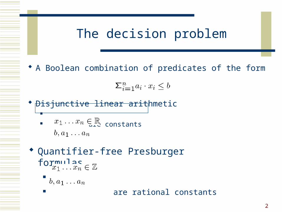
The decision problem

A Boolean combination of predicates of the form

Disjunctive linear arithmetic

are constants

Quantifier-free Presburger formulas

are rational constants

3

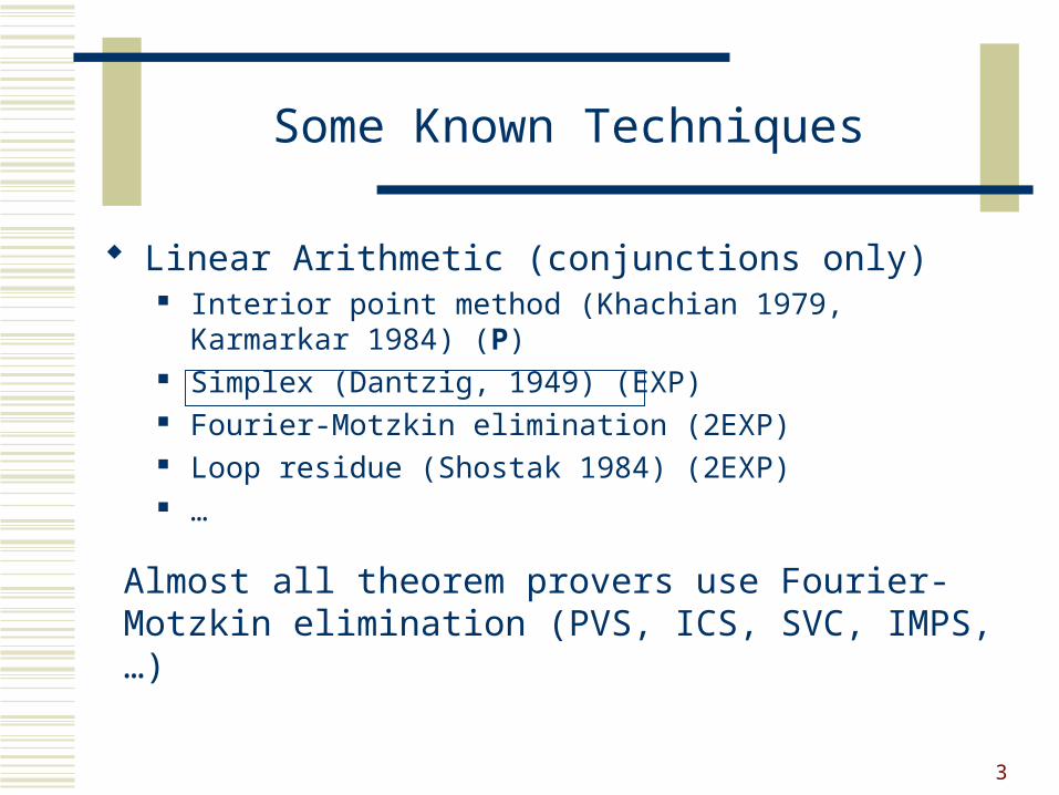
Some Known Techniques

Linear Arithmetic (conjunctions only) Interior point method (Khachian 1979, Karmarkar 1984) (P) Simplex (Dantzig, 1949) (EXP) Fourier-Motzkin elimination (2EXP) Loop residue (Shostak 1984) (2EXP) …

Almost all theorem provers use Fourier-Motzkin elimination (PVS, ICS, SVC, IMPS, …)

4

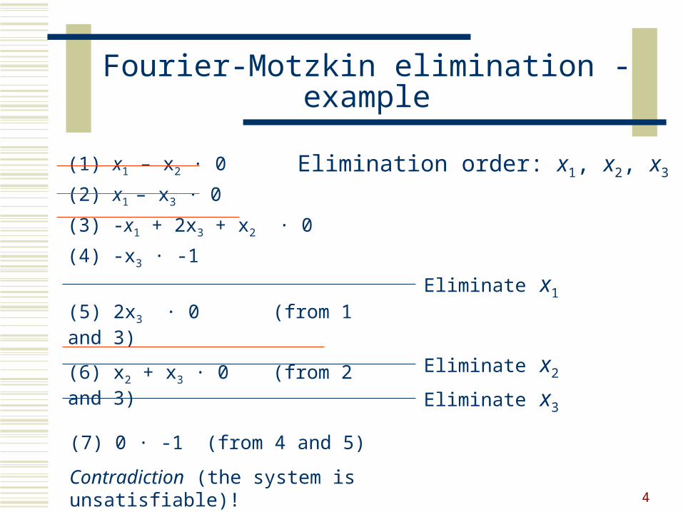
Fourier-Motzkin elimination - example

(1) x1 – x2 · 0

(2) x1 – x3 · 0

(3) -x1 + 2x3 + x2 · 0

(4) -x3 · -1

Eliminate x1

Eliminate x2

Eliminate x3

(5) 2x3 · 0 (from 1 and 3)

(6) x2 + x3 · 0 (from 2 and 3)

(7) 0 · -1 (from 4 and 5)

Contradiction (the system is unsatisfiable)!

Elimination order: x1, x2, x3

5

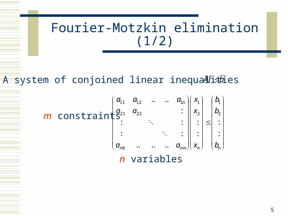
Fourier-Motzkin elimination (1/2)

nnmnm

n

b

b

b

x

x

x

aa

aa

aaa

:

:

:

:

......

::

::

:

....

2

1

2

1

1

2221

11211

bIA A system of conjoined linear inequalities

m constraints

n variables

6

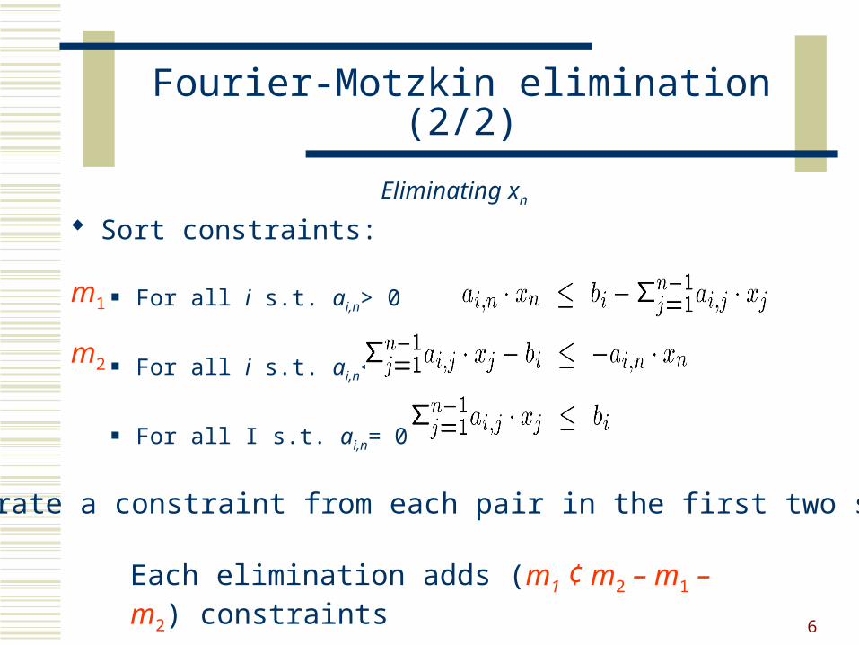
Fourier-Motzkin elimination (2/2)

Sort constraints:

For all i s.t. ai,n> 0

For all i s.t. ai,n< 0

For all I s.t. ai,n= 0

Each elimination adds (m1 ¢ m2 – m1 – m2) constraints

m1

m2

Eliminating xn

Generate a constraint from each pair in the first two sets.

7

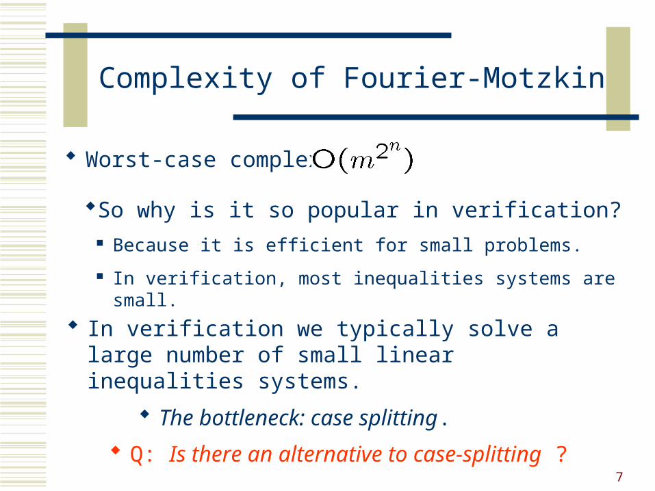
Complexity of Fourier-Motzkin

Worst-case complexity:

Q: Is there an alternative to case-splitting ?

So why is it so popular in verification? Because it is efficient for small problems.

In verification, most inequalities systems are small.

In verification we typically solve a large number of small linear inequalities systems.

The bottleneck: case splitting.

8

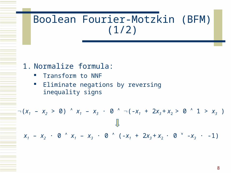
Boolean Fourier-Motzkin (BFM) (1/2)

x1 – x2 · 0 x1 – x3 · 0 (-x1 + 2x3 + x2 · 0 -x3 · -1)

(x1 – x2 > 0) x1 – x3 · 0 (-x1 + 2x3 + x2 > 0 1 > x3 )

1. Normalize formula: Transform to NNF Eliminate negations by reversing inequality signs

9

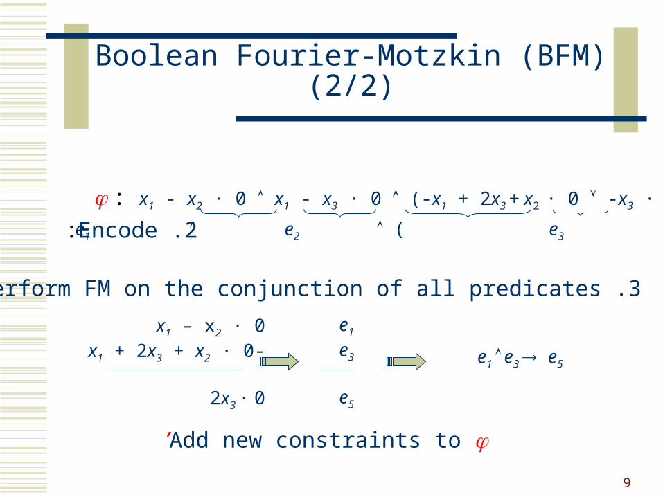
: x1 - x2 · 0 x1 - x3 · 0 (-x1 + 2x3 + x2 · 0 -x3 · -1)

2. Encode :

Boolean Fourier-Motzkin (BFM) (2/2)

3 .Perform FM on the conjunction of all predicates:

’: e1 e2 ( e3 e4 )

x1 – x2 · 0-x1 + 2x3 + x2 · 0

2x3 · 0

e1

e3

e5

e1 e3 e5

Add new constraints to ’

10

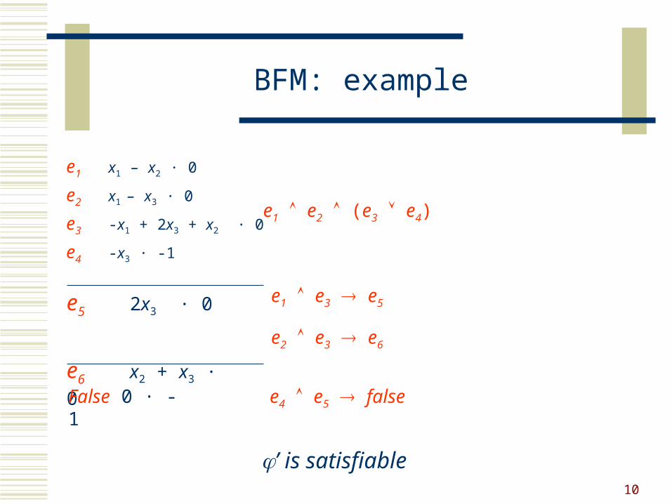
BFM: example

e1 x1 – x2 · 0

e2 x1 – x3 · 0

e3 -x1 + 2x3 + x2 · 0

e4 -x3 · -1

e1 e2 (e3 e4)

e5 2x3 · 0

e6 x2 + x3 · 0

e1 e3 e5

e2 e3 e6

False 0 · -1 e4 e5 false

’ is satisfiable

11

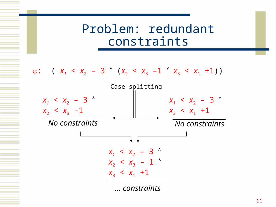
Problem: redundant constraints

: ( x1 < x2 – 3 (x2 < x3 –1 x3 < x1 +1))

Case splitting

x1 < x2 – 3 x2 < x3 –1

x1 < x2 – 3 x3 < x1 +1

No constraints No constraints

x1 < x2 – 3 x2 < x3 – 1 x3 < x1 +1

... constraints

12

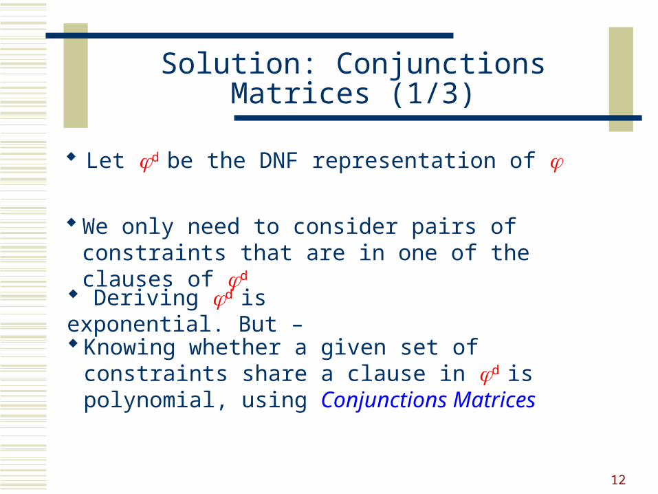
Let d be the DNF representation of

Solution: Conjunctions Matrices (1/3)

We only need to consider pairs of constraints that are in one of the clauses of d

Deriving d is exponential. But –

Knowing whether a given set of constraints share a clause in d is polynomial, using Conjunctions Matrices

13

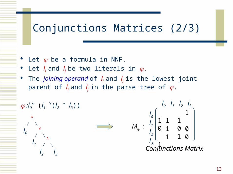
Conjunctions Matrices (2/3)

Let be a formula in NNF. Let li and lj be two literals in .

The joining operand of li and lj is the lowest joint parent of li and lj in the parse tree of .

:l0 (l1 (l2 l3))

l0

l1

l2 l3

l0 l1 l2 l3

l0

l1

l2

l3

1 1 1 1 0 0 1 0 1 1 0 1

Conjunctions Matrix

M :

14

Claim 1: A set of literals L={l0,l1…ln} share a clause in d

if and only if for all li,lj L, ij, M[li,lj] =1.

Conjunctions Matrices (3/3)

We can now consider only pairs of constraints that their corresponding entry in M is equal to 1

15

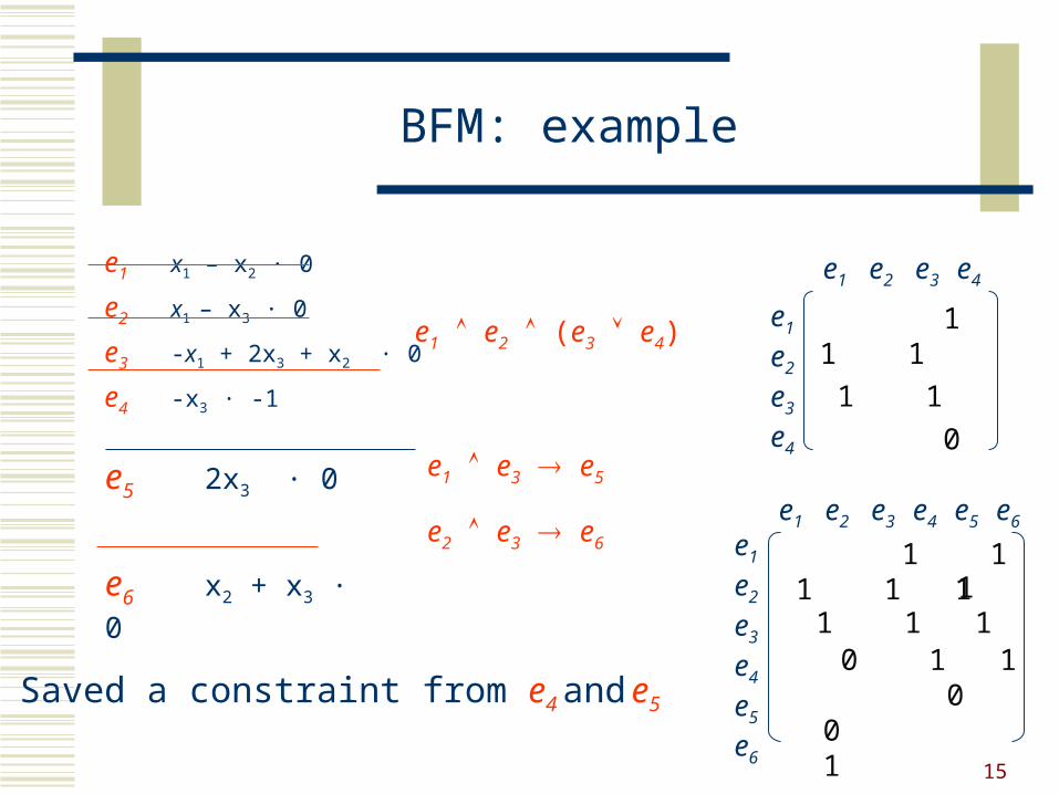
BFM: example

e1 x1 – x2 · 0

e2 x1 – x3 · 0

e3 -x1 + 2x3 + x2 · 0

e4 -x3 · -1

e1 e2 (e3 e4)

e1 e2 e3 e4

e1

e2

e3

e4

1 1 1

1 1

0

e5 2x3 · 0

e6 x2 + x3 · 0

e1 e3 e5

e2 e3 e6

e1 e2 e3 e4 e5 e6

e1

e2

e3

e4

e5

e6

1 1 1 1 1 1 1 1 1 0 1 1 0 0 1

Saved a constraint from e4 and e5

16

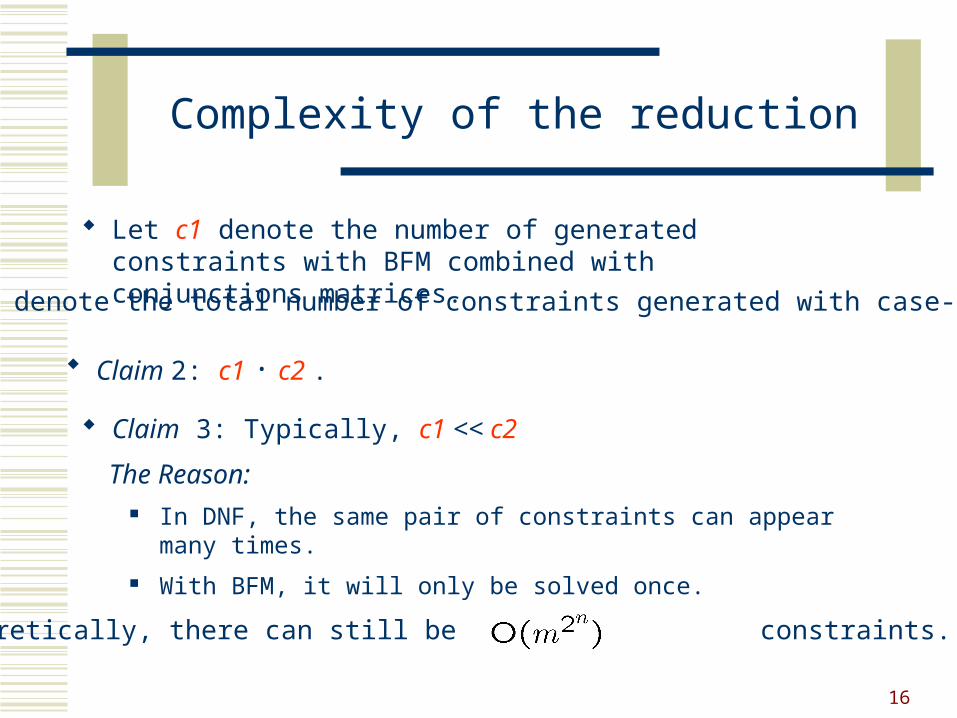
Complexity of the reduction

Claim 3: Typically, c1 << c2

The Reason: In DNF, the same pair of constraints can appear many times.

With BFM, it will only be solved once.

Theoretically, there can still be constraints.

Let c1 denote the number of generated constraints with BFM combined with conjunctions matrices.

Let c2 denote the total number of constraints generated with case-splitting.

Claim 2: c1 · c2 .

17

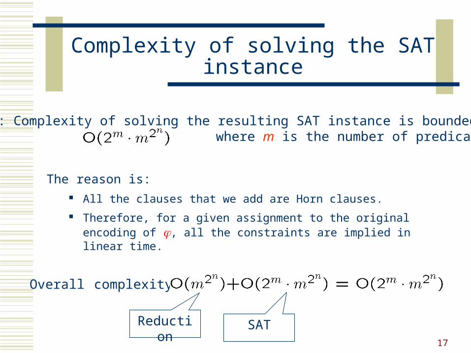
The reason is: All the clauses that we add are Horn clauses.

Therefore, for a given assignment to the original encoding of , all the constraints are implied in linear time.

Complexity of solving the SAT instance

Claim 4: Complexity of solving the resulting SAT instance is bounded by where m is the number of predicates in

Overall complexity:

Reduction SAT

18

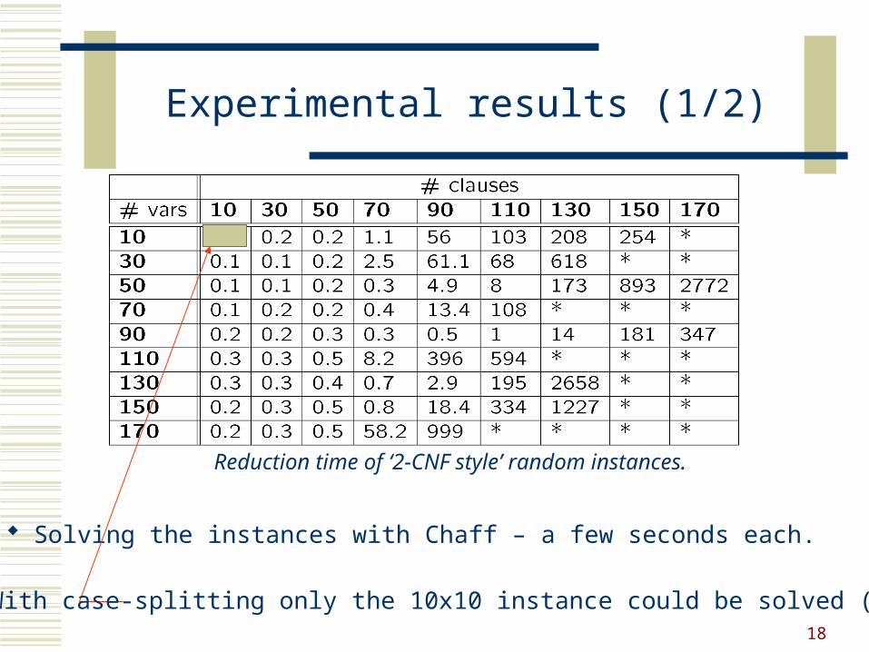
Experimental results (1/2)

Reduction time of ‘2-CNF style’ random instances.

Solving the instances with Chaff – a few seconds each.

With case-splitting only the 10x10 instance could be solved (~600 sec.)

19

Experimental results (2/2)

Seven Hardware designs with equalities and inequalities All seven solved with BFM in a few seconds Five solved with ICS in a few seconds. The other two could not be

solved.

The reason (?):ICS has a more efficient implementation of Fourier-Motzkin compared to PORTA

On the other hand…

Standard ICS benchmarks (A conjunction of inequalities) Some could not be solved with BFM

…while ICS solves all of them in a few seconds.

20

Some Known Techniques

Quantifier-free Presburger formulas Branch and Bound SUP-INF (Bledsoe 1974) Omega Test (Pugh 1991) …

21

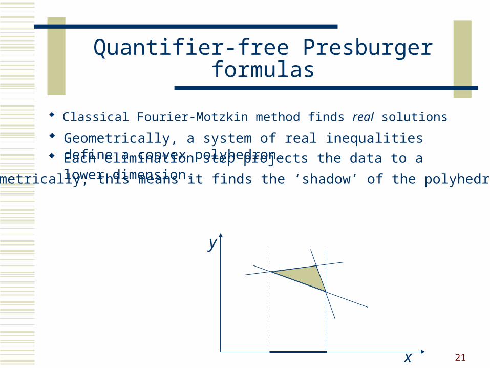
Quantifier-free Presburger formulas

Classical Fourier-Motzkin method finds real solutions

x

y

Geometrically, a system of real inequalities define a convex polyhedron. Each elimination step projects the data to a lower dimension.

Geometrically, this means it finds the ‘shadow’ of the polyhedron.

22

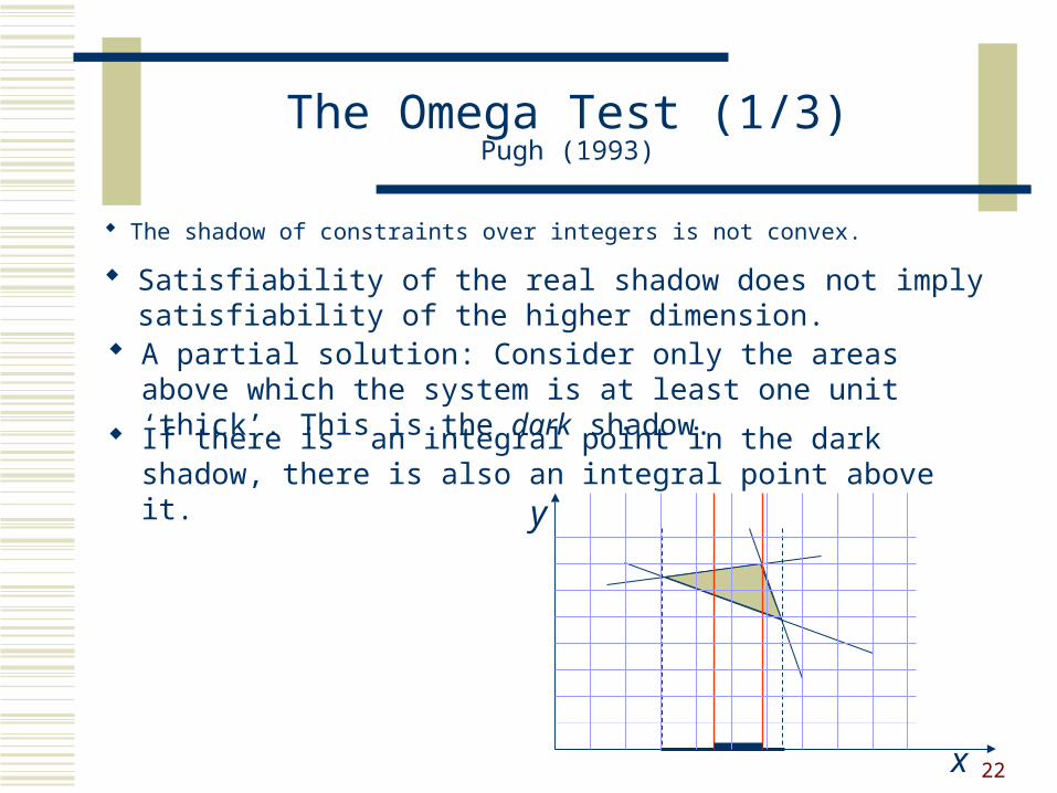
The Omega Test (1/3)Pugh (1993)

The shadow of constraints over integers is not convex.

x

y

Satisfiability of the real shadow does not imply satisfiability of the higher dimension.

A partial solution: Consider only the areas above which the system is at least one unit ‘thick’. This is the dark shadow.

If there is an integral point in the dark shadow, there is also an integral point above it.

23

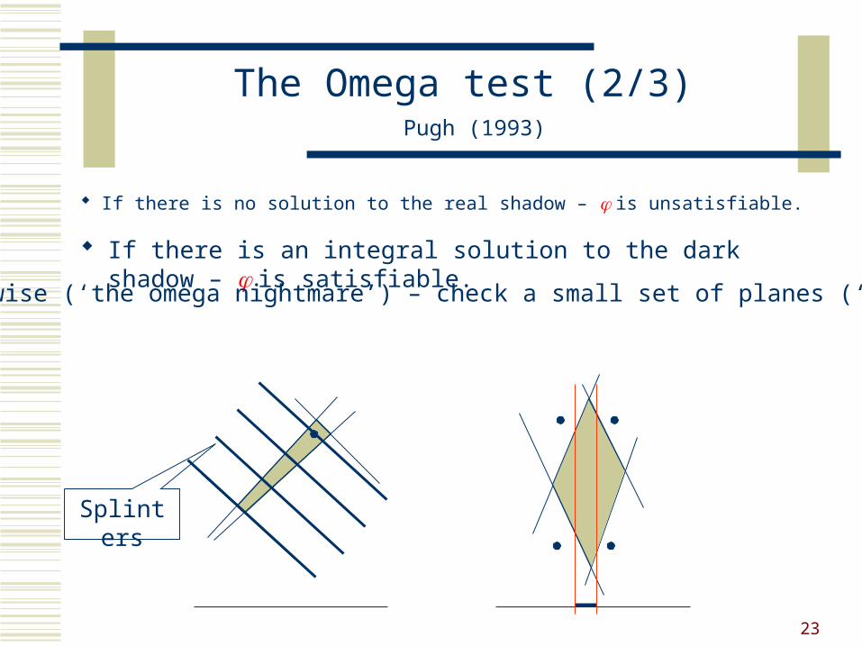
The Omega test (2/3) Pugh (1993)

If there is no solution to the real shadow – is unsatisfiable.

Splinters

If there is an integral solution to the dark shadow – is satisfiable.

Otherwise (‘the omega nightmare’) – check a small set of planes (‘splinters’).

24

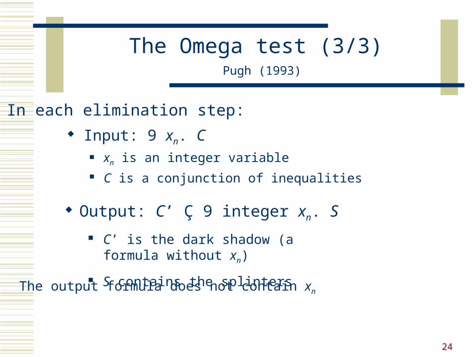
The Omega test (3/3) Pugh (1993)

Input: 9 xn. C xn is an integer variable C is a conjunction of inequalities

In each elimination step:

The output formula does not contain xn

Output: C’ Ç 9 integer xn. S

C’ is the dark shadow (a formula without xn)

S contains the splinters

25

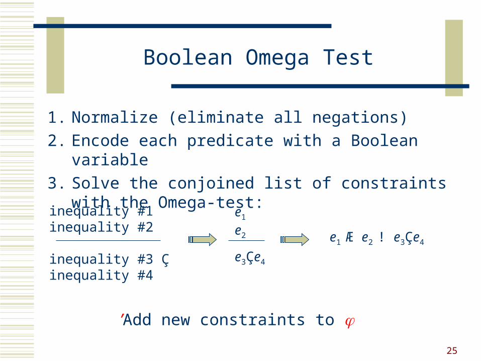
Boolean Omega Test

1. Normalize (eliminate all negations)

2. Encode each predicate with a Boolean variable

3. Solve the conjoined list of constraints with the Omega-test:

Add new constraints to ’

inequality #1inequality #2

inequality #3 Çinequality #4

e1

e2

e3Çe4

e1 Æ e2 ! e3Çe4

26

Related work

A reduction to SAT is not the only way …

27

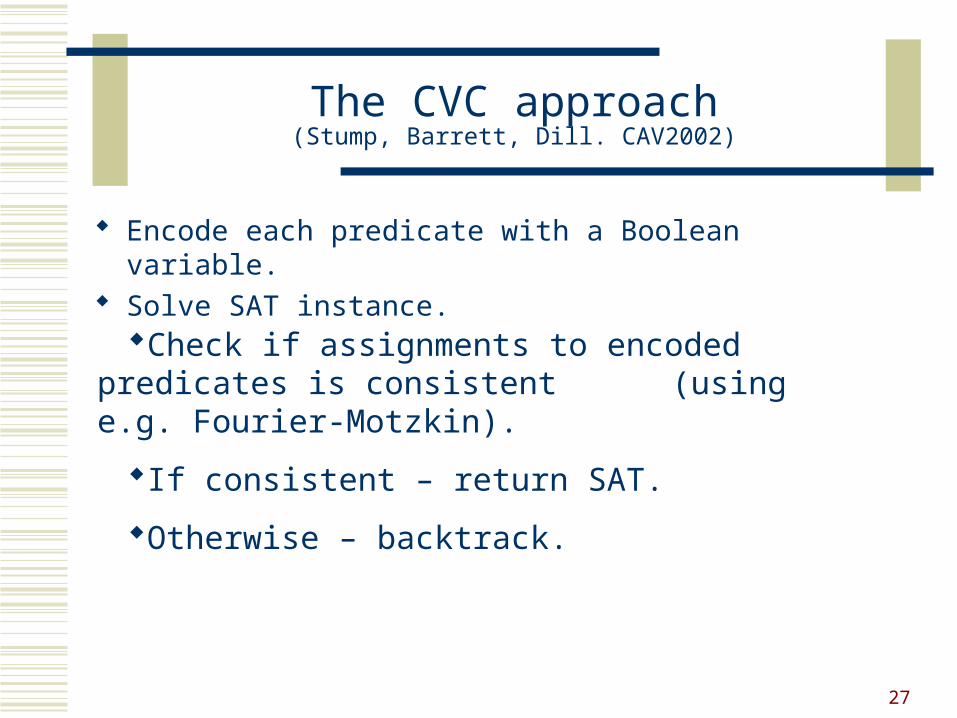
The CVC approach(Stump, Barrett, Dill. CAV2002)

Encode each predicate with a Boolean variable. Solve SAT instance.

Check if assignments to encoded predicates is consistent (using e.g. Fourier-Motzkin).

If consistent – return SAT.

Otherwise – backtrack.

28

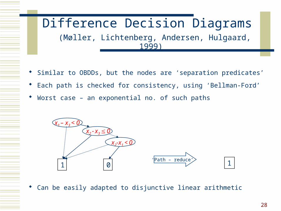
Difference Decision Diagrams (Møller, Lichtenberg, Andersen, Hulgaard, 1999)

Similar to OBDDs, but the nodes are ‘separation predicates’

Each path is checked for consistency, using ‘Bellman-Ford’

Worst case – an exponential no. of such paths

x1 – x3 < 0x2 - x3 0

x2-x1 < 0

1 0 1‘Path – reduce’

Can be easily adapted to disjunctive linear arithmetic

29

Finite domain instantiation

Disjunctive linear arithmetic and its sub-theories enjoy the ‘small model property’.

A known sufficient domain for equality logic: 1..n (where n is the number of variables).

For this logic, it is possible to compute a significantly smaller domain for each variable (Pnueli et al., 1999).

The algorithm is a graph-based analysis of the formula structure.

Potentially can be extended to linear arithmetic.

30

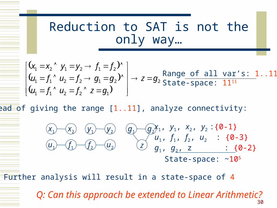
Reduction to SAT is not the only way…

Instead of giving the range [1..11], analyze connectivity:

x1 x2 y1 y2 g1 g2

zu1 f1 f2 u2

Further analysis will result in a state-space of 4

2

12211

212211

212121

gz

gzfufu

ggfufu

ffyyxx

Range of all var’s: 1..11State-space: 1111

x1, y1, x2, y2 :{0-1}u1, f1, f2, u2 : {0-3}g1, g2, z : {0-2}

State-space: ~105

Q: Can this approach be extended to Linear Arithmetic?