Embed Size (px)
Citation preview
Ofer Strichman, Technion 1
Decision Procedures in First Order Logic
Part III – Decision Procedures for Equality Logic and Uninterpreted Functions
Technion 2
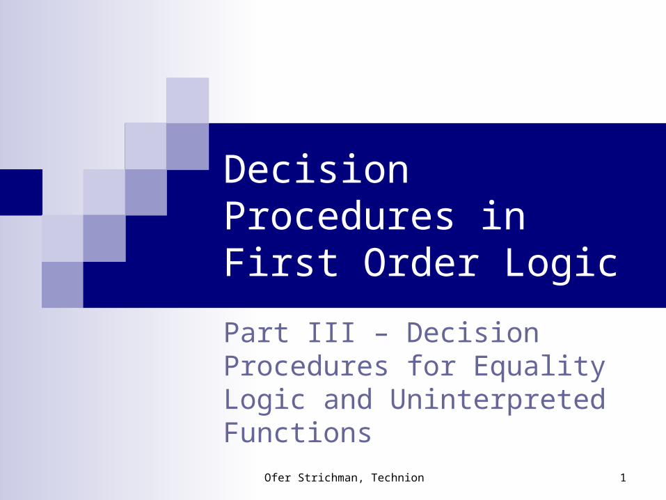
Part I - Introduction Reminders -
What is Logic Proofs by deduction Proofs by enumeration Decidability, Soundness and Completeness Some notes on Propositional Logic
Deciding Propositional Logic SAT tools BDDs
Technion 3
Part II – Introduction to Equality Logic and Uninterpreted Functions
Introduction Definition, complexity Reducing Uninterpreted Functions to Equality Logic Using Uninterpreted Functions in proofs Simplifications
Introduction to the decision procedures The framework: assumptions and Normal Forms General terms and notions Solving a conjunction of equalities Simplifications

Technion 4
Part III – Decision Procedures for Equality Logic and Uninterpreted Functions
Algorithm I – From Equality to Propositional Logic Adding transitivity constraints Making the graph chordal An improved procedure: consider polarity
Algorithm II – Range-Allocation What is the small-model property? Finding a small adequate range (domain) to each variable Reducing to Propositional Logic
Technion 5
We will first investigate methods that solve Equality Logic. Uninterpreted functions are eliminated with one of the reduction schemes.
Our starting point: the E-Graph GE(E)
Recall: GE(E) represents an abstraction of E:
It represents ALL equality formulas with the same set of equality predicates as E
Decision Procedures for Equality Logic
Technion 6
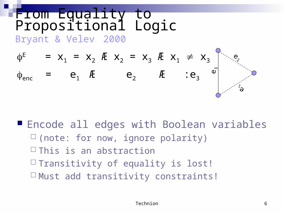
From Equality to Propositional LogicBryant & Velev 2000
E = x1 = x2 Æ x2 = x3 Æ x1 x3
enc = e1 Æ e2 Æ :e3
Encode all edges with Boolean variables (note: for now, ignore polarity) This is an abstraction Transitivity of equality is lost! Must add transitivity constraints!
e 3
e2
e1
Technion 7
From Equality to Propositional Logic
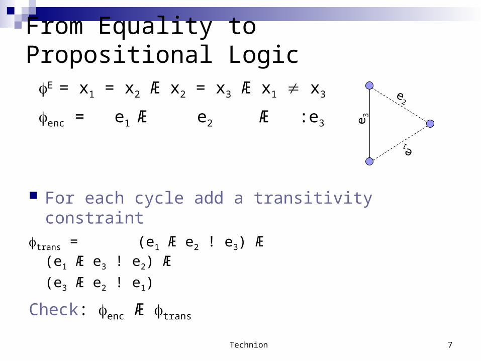
E = x1 = x2 Æ x2 = x3 Æ x1 x3
enc = e1 Æ e2 Æ :e3
For each cycle add a transitivity constrainttrans = (e1 Æ e2 ! e3) Æ
(e1 Æ e3 ! e2) Æ
(e3 Æ e2 ! e1)
Check: enc Æ trans
e 3
e2
e1
Technion 8
From Equality to Propositional Logic
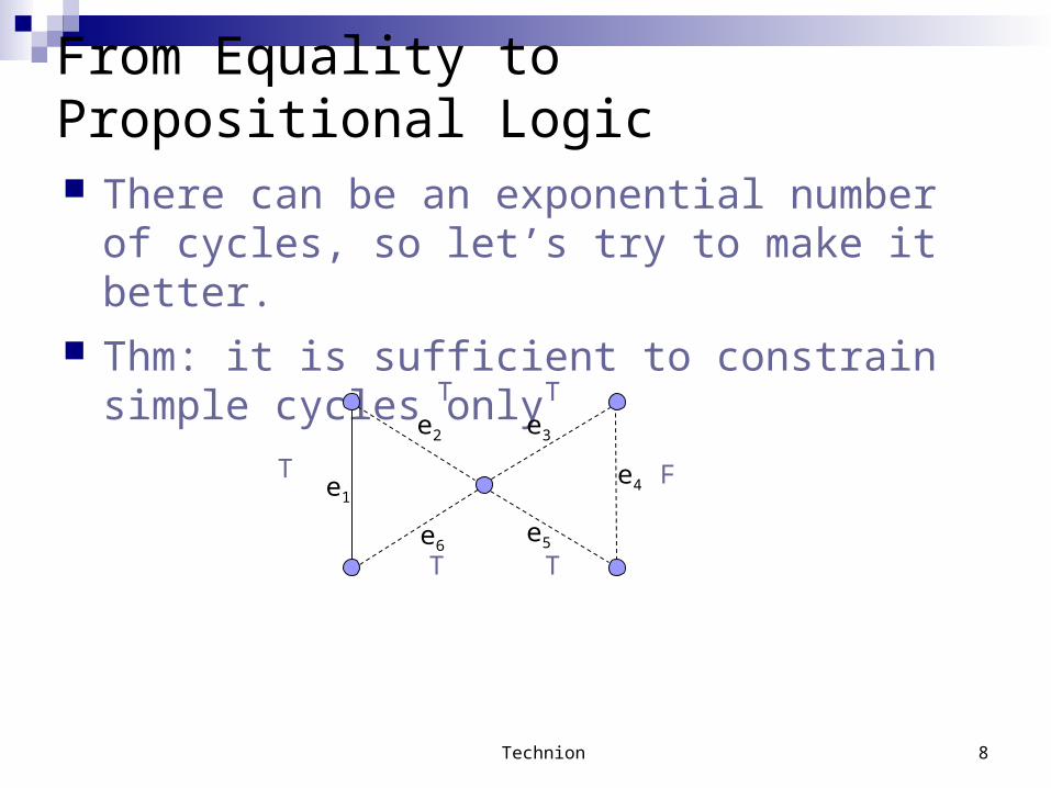
There can be an exponential number of cycles, so let’s try to make it better.
Thm: it is sufficient to constrain simple cycles only
e1
e2 e3
e4
e5e6
T
T T
TT
F
Technion 9
From Equality to Propositional Logic
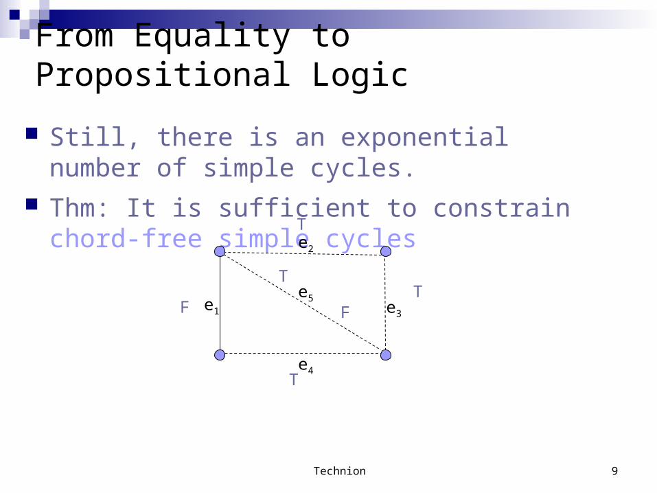
Still, there is an exponential number of simple cycles. Thm: It is sufficient to constrain chord-free simple
cycles
e1
e2
e3
e4
e5
T
T
T
F
T
F
Technion 10
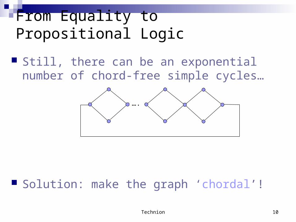
Still, there can be an exponential number of chord-free simple cycles…
Solution: make the graph ‘chordal’!
From Equality to Propositional Logic
….
Technion 11
From Equality to Propositional Logic
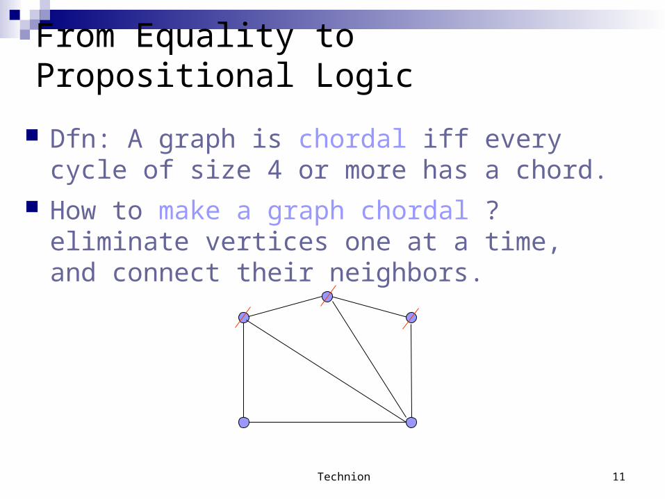
Dfn: A graph is chordal iff every cycle of size 4 or more has a chord.
How to make a graph chordal ? eliminate vertices one at a time, and connect their neighbors.
Technion 12
From Equality to Propositional Logic
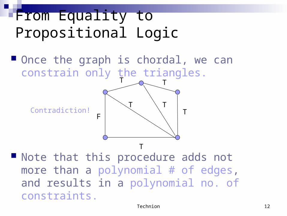
Once the graph is chordal, we can constrain only the triangles.
Note that this procedure adds not more than a polynomial # of edges, and results in a polynomial no. of constraints.
T
T
TT
F
TTContradiction!
Technion 13
Improvement
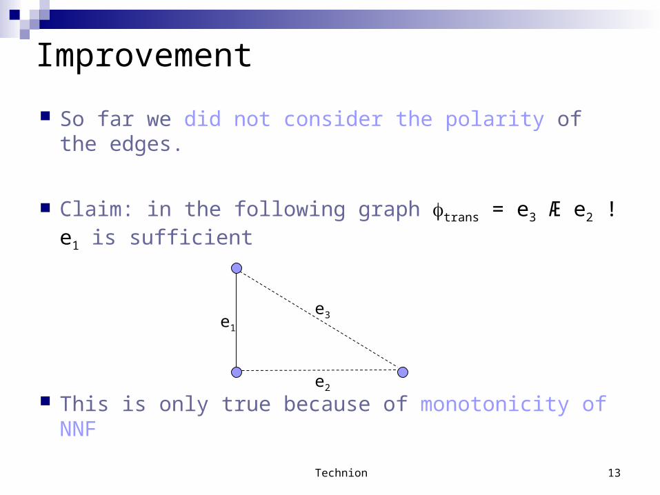
So far we did not consider the polarity of the edges.
Claim: in the following graph trans = e3 Æ e2 ! e1 is sufficient
This is only true because of monotonicity of NNF
e1
e2
e3

Technion 14
Definitions
Let C = (es,e1,…,en) where es is solid and e1,…,en are dashed be a simple (contradictory) cycle.
Let be a formula over the Boolean variables encoding C
We say that C is constrained in with respect to es iff every assignment s.t. (es) = F and
(e1) = …=(en) = T
contradicts
Technion 15
A theorem
Let ’trans constrain all simple contradictory cycles with respect to their solid edges.
Thm: E is satisfiable iff enc Æ ’trans is satisfiable.
Proof strategy: Let ’ be a satisfying assignment to enc Æ ’trans
We will construct that satisfies enc Æ trans
Technion 24
Improved procedure
How can we use the theorem without enumerating contradictory cycles ?
Answer: Consider the chordal graph. Add constraints to triangles only if necessary to enforce
transitivity of contradictory cycles How?... read the lecture notes.
Technion 25
Part III – Decision Procedures for Equality Logic and Uninterpreted Functions
Algorithm I – From Equality to Propositional Logic Adding transitivity constraints Making the graph chordal An improved procedure: consider polarity
Algorithm II – Range-Allocation What is the small-model property? Finding a small adequate range (domain) to each variable Reducing to Propositional Logic
Technion 26
Range allocation
The small model property Range Allocation
Technion 27
u x y u x y z u u
z x y x y1 1 1 2 2 2 1 2
1 1 2 2
( ) ( )
u F x y u F x y z G u u
z G F x y F x y1 1 1 2 2 2 1 2
1 1 2 2
( , ) ( , ) ( , )
( ( , ), ( , ))
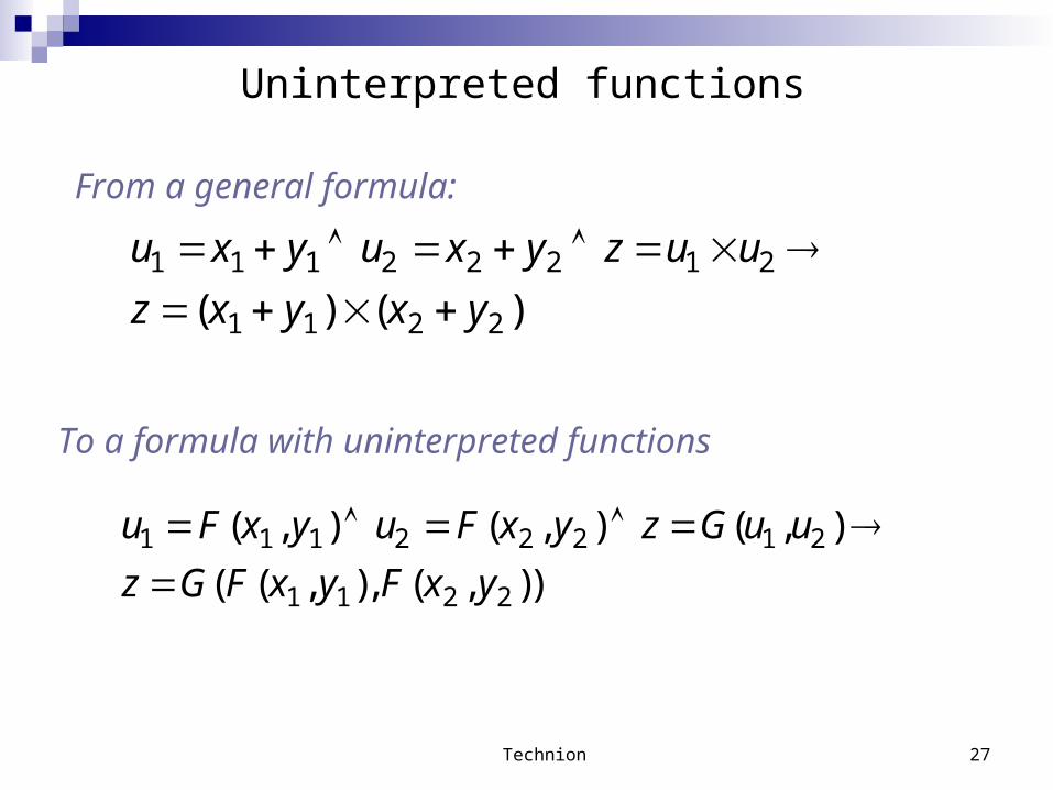
To a formula with uninterpreted functions
Uninterpreted functions
From a general formula:
Technion 28
u F x y u F x y z G u u
z G F x y F x y1 1 1 2 2 2 1 2
1 1 2 2
( , ) ( , ) ( , )
( ( , ), ( , ))
2
12211
212211
212121
gz
gzfufu
ggfufu
ffyyxx
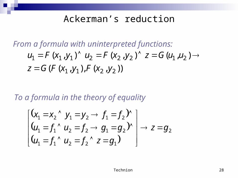
From a formula with uninterpreted functions:
To a formula in the theory of equality
Ackerman’s reduction
Technion 29
The Small Model Property
Equality Logic enjoys the Small Model Property This means that if a formula in this logic is
satisfiable, then there is a finite, bounded in size, model that satisfies it.
It gets better: in Equality Logic we can compute this bound, which suggests a decision procedure.
What is this bound?
Technion 30
The Small Model Property
Claim: the range 1..n is adequate, where n is the number of variables in
Proof: Every satisfying assignment defines a partition of the
variables Every assignment that results in the same partitioning
also satisfies the formula The range 1..n allows all partitionings
Technion 31
Complexity
We need log n variables to encode the range 1…n For n variables we need n log n bits. This is already better than the worst-case O(n2) bits
required by the Boolean encoding method …
Technion 32
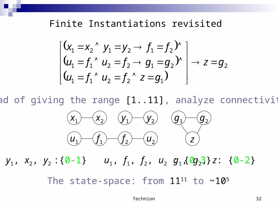
Instead of giving the range [1..11], analyze connectivity:
x1 x2 y1 y2 g1 g2
zu1 f1 f2 u2
x1, y1, x2, y2 :{0-1} u1, f1, f2, u2 : {0-3} g1, g2, z: {0-2}
The state-space: from 1111 to ~105
2
12211
212211
212121
gz
gzfufu
ggfufu
ffyyxx
Finite Instantiations revisited
Technion 33
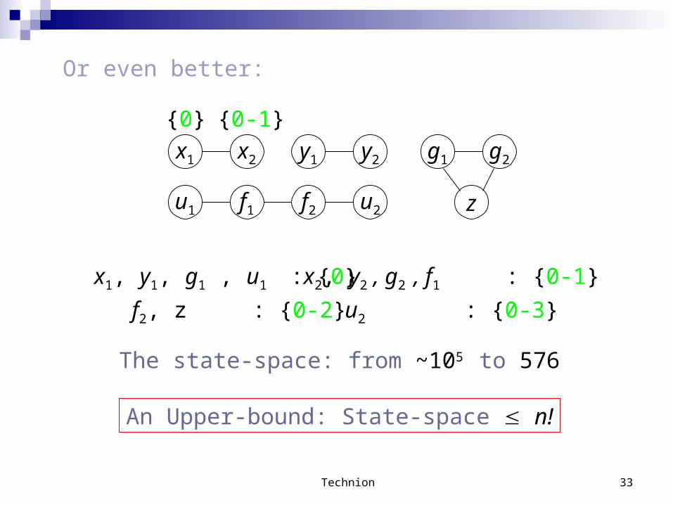
Or even better:
x1 x2 y1 y2 g1 g2
zu1 f1 f2 u2
x1, y1, g1 , u1 : {0}
{0} {0-1}
An Upper-bound: State-space n!
x2, y2 , g2 , f1 : {0-1}
u2 : {0-3} f2, z : {0-2}
The state-space: from ~105 to 576
Technion 34
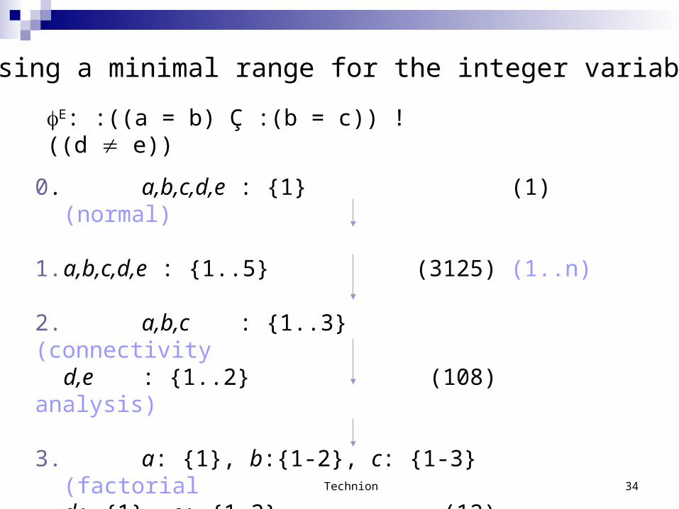
Choosing a minimal range for the integer variables
0. a,b,c,d,e : {1} (1) (normal)
1. a,b,c,d,e : {1..5} (3125) (1..n)
2. a,b,c : {1..3} (connectivity d,e : {1..2} (108) analysis)
3. a: {1}, b:{1-2}, c: {1-3} (factoriald: {1}, e: {1-2} (12) reduction)
4. ... ... ...
E: :((a = b) Ç :(b = c)) !((d e))
Technion 35
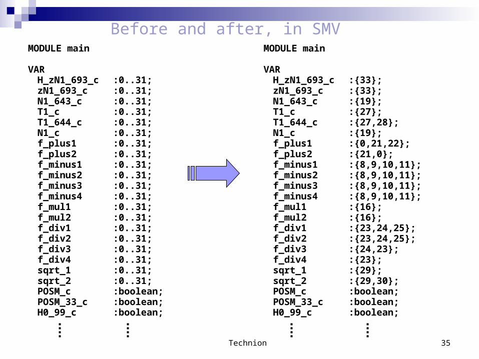
MODULE main VAR H_zN1_693_c :0..31; zN1_693_c :0..31; N1_643_c :0..31; T1_c :0..31; T1_644_c :0..31; N1_c :0..31; f_plus1 :0..31; f_plus2 :0..31; f_minus1 :0..31; f_minus2 :0..31; f_minus3 :0..31; f_minus4 :0..31; f_mul1 :0..31; f_mul2 :0..31; f_div1 :0..31; f_div2 :0..31; f_div3 :0..31; f_div4 :0..31; sqrt_1 :0..31; sqrt_2 :0..31; POSM_c :boolean; POSM_33_c :boolean; H0_99_c :boolean;
MODULE main VAR H_zN1_693_c :{33}; zN1_693_c :{33}; N1_643_c :{19}; T1_c :{27}; T1_644_c :{27,28}; N1_c :{19}; f_plus1 :{0,21,22}; f_plus2 :{21,0}; f_minus1 :{8,9,10,11}; f_minus2 :{8,9,10,11}; f_minus3 :{8,9,10,11}; f_minus4 :{8,9,10,11}; f_mul1 :{16}; f_mul2 :{16}; f_div1 :{23,24,25}; f_div2 :{23,24,25}; f_div3 :{24,23}; f_div4 :{23}; sqrt_1 :{29}; sqrt_2 :{29,30}; POSM_c :boolean; POSM_33_c :boolean; H0_99_c :boolean;
Before and after, in SMV
Technion 36
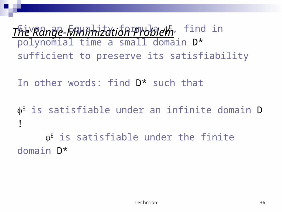
The Range-Minimization Problem
Given an Equality formula E, find in polynomial time a small
domain D* sufficient to preserve its satisfiability
In other words: find D* such that
E is satisfiable under an infinite domain D !
E is satisfiable under the finite domain D*
Technion 37
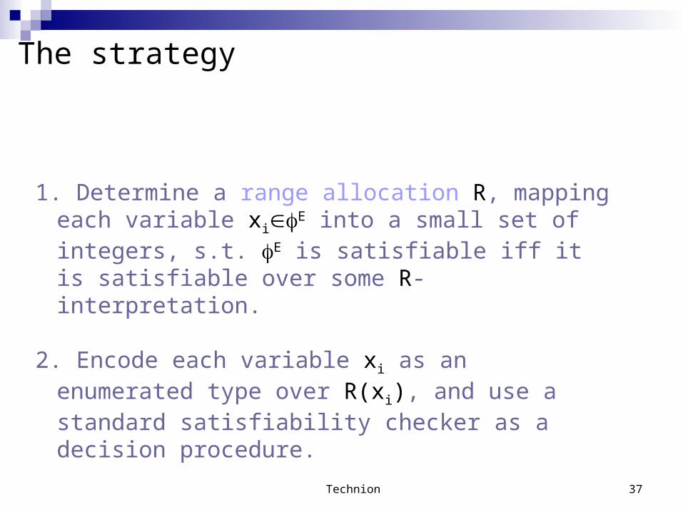
The strategy
1. Determine a range allocation R, mapping each variable xiE into a small set of integers, s.t. E is satisfiable iff it is satisfiable over some R-interpretation.
2. Encode each variable xi as an enumerated type over R(xi), and use a standard satisfiability checker as a decision procedure.
Technion 38
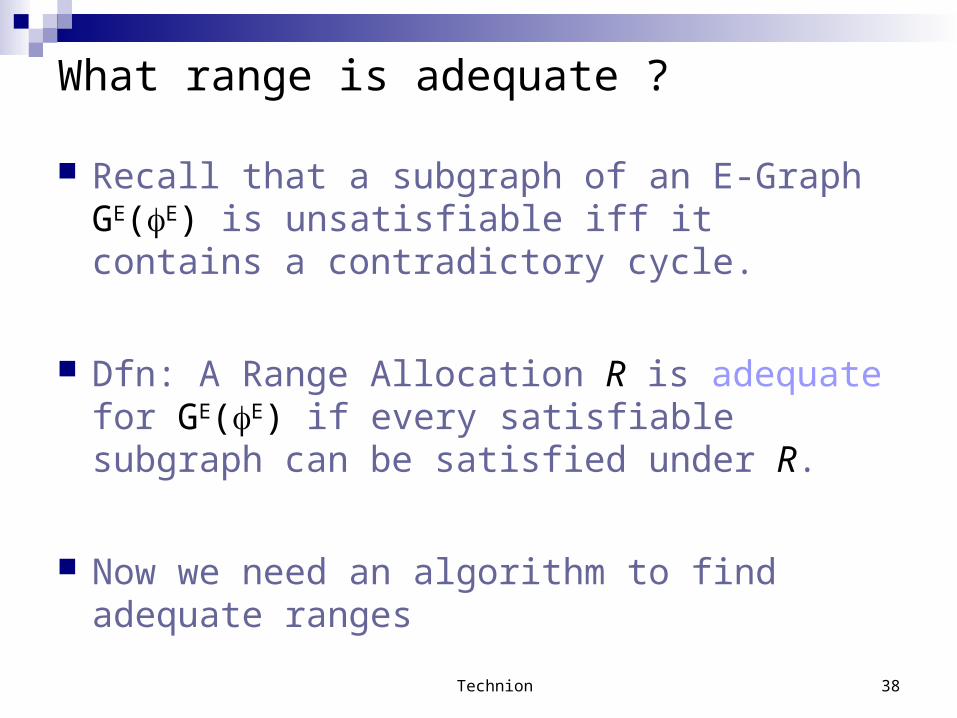
What range is adequate ?
Recall that a subgraph of an E-Graph GE(E) is unsatisfiable iff it contains a contradictory cycle.
Dfn: A Range Allocation R is adequate for GE(E) if every satisfiable subgraph can be satisfied under R.
Now we need an algorithm to find adequate ranges
Technion 39
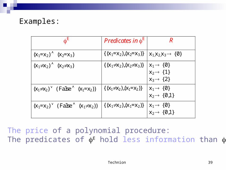
Examples:
E Predicates in E R
(x1=x2) (x2=x3) {(x1=x2),(x2=x3)} x1,x2,x3 {0}
(x1x2) (x2x3) {(x1x2),(x2x3)} x1 {0} x2 {1} x3 {2}
(x1x2) ( False (x1=x2)) {(x1x2),(x1=x2)} x1 {0} x2 {0,1}
(x1=x2) ( False (x1x2)) {(x1x2),(x1=x2)} x1 {0} x2 {0,1}
The price of a polynomial procedure: The predicates of E hold less information than E .
Technion 40
x1 x2 y1 y2 g1 g2
zu1 f1 f2 u2
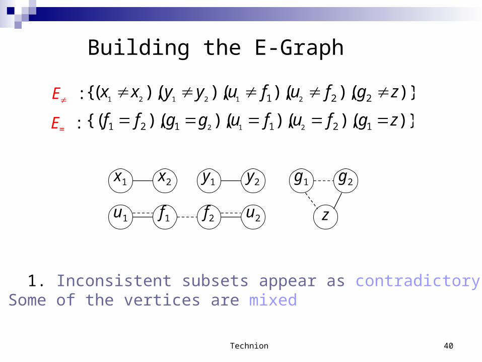
Building the E-Graph
)}(),(),(),(),({ 221 212121zgfufuyyxx
)}(),(),(),(),{( 121121 212zgfufuggff
E :
E= :
Note: 1. Inconsistent subsets appear as contradictory cycles2. Some of the vertices are mixed
Technion 41
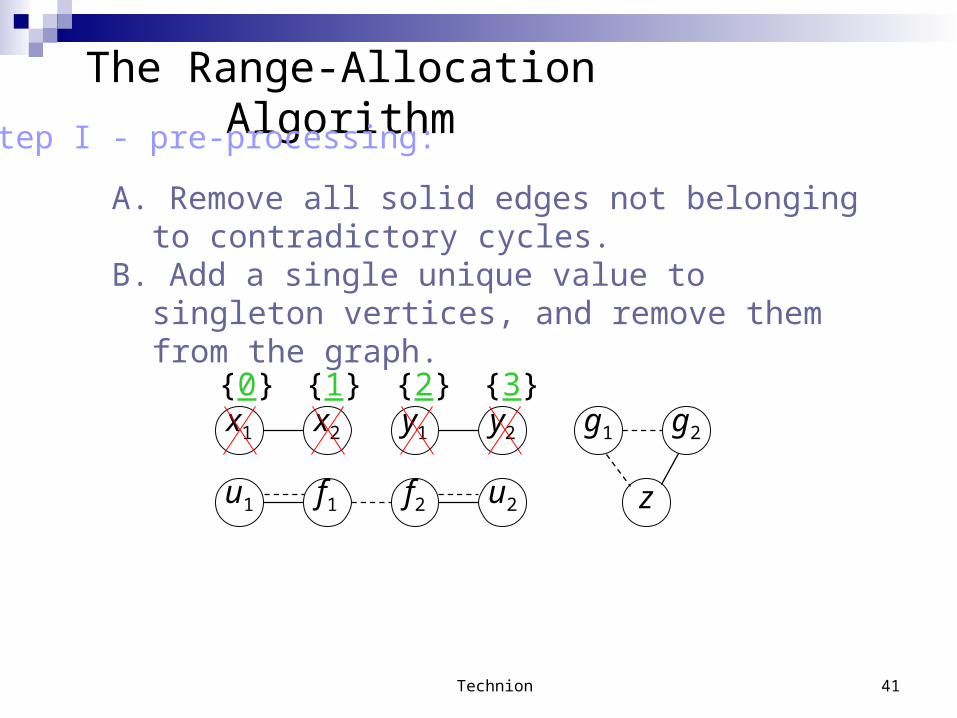
The Range-Allocation Algorithm
A. Remove all solid edges not belonging to contradictory cycles.
B. Add a single unique value to singleton vertices, and remove them from the graph.
x1 x2 y1 y2 g1 g2
zu1 f1 f2 u2
{0} {1} {3}{2}
Step I - pre-processing:
Technion 42
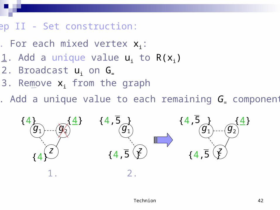
Step II - Set construction:
A. For each mixed vertex xi:
1. Add a unique value ui to R(xi)2. Broadcast ui on G=
3. Remove xi from the graph
B. Add a unique value to each remaining G= component
g1 g2
z
{4}{4}
{4}
g1
z
{4, }
{4, }
g1 g2
z
{4}
{4, }
{4, }
1. 2.
5
5
5
5
Technion 43
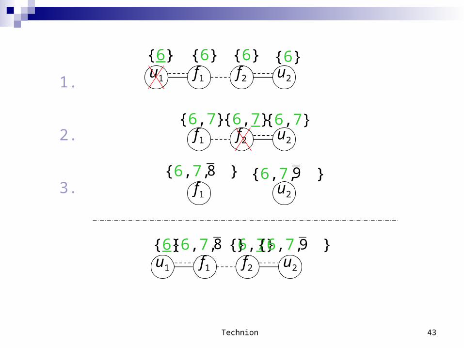
u1 f1 f2 u2
{6} {6} {6} {6}
f1 f2 u2
{6,7} {6,7} {6,7}
u2
{6,7, }
u1 f1 f2 u2
{6} {6,7}
1.
2.
3. f1
{6,7, }
{6,7, } {6,7, }
8
8
9
9
Technion 44
x1 x2 y1 y2 g1 g2
zu1 f1 f2 u2
{3}{2} {4}
{4, }
{4, }
{6} {6,7}{6,7, } {6,7, }
{1}{0} 5
58 9
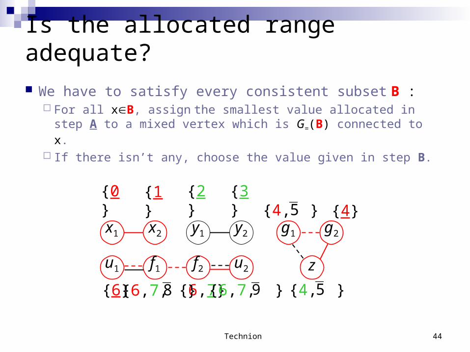
Is the allocated range adequate?
We have to satisfy every consistent subset B : For all xB, assign the smallest value allocated in step A
to a mixed vertex which is G=(B) connected to x.
If there isn’t any, choose the value given in step B.

Technion 45
Further optimizations
The order in which mixed vertices are eliminated has a strong effect.
Not all mixed vertices need to start from a unique value. An analysis that involves solving a coloring problem can help here…
… (see lecture notes)
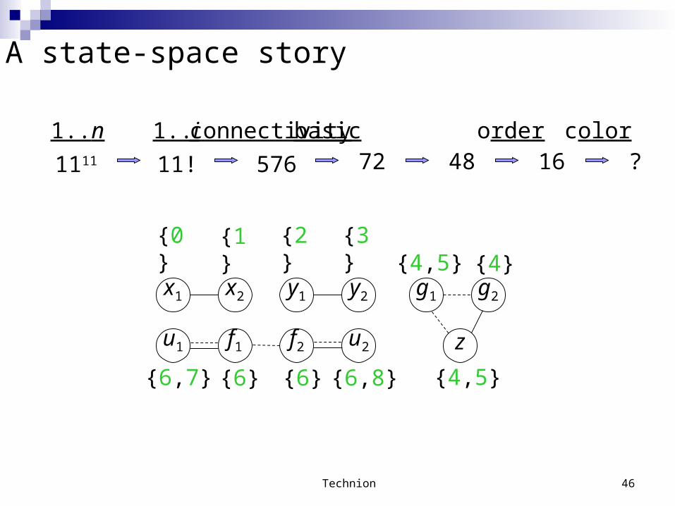
Technion 46
x1 x2 y1 y2 g1 g2
zu1 f1 f2 u2
{3}{2} {4}
{4,5}
{4,5}
{6,7} {6}{6} {6,8}
{1}{0}
A state-space story
1111 11! 161..n 1..i basic order color
4872 ?576
connectivity
Technion 47
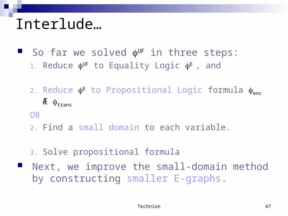
Interlude…
So far we solved UF in three steps:1. Reduce UF to Equality Logic E , and
2. Reduce E to Propositional Logic formula enc Æ trans
OR
2. Find a small domain to each variable.
3. Solve propositional formula
Next, we improve the small-domain method by constructing smaller E-graphs.
Technion 48
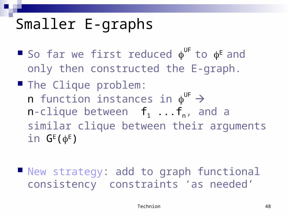
Smaller E-graphs
So far we first reduced UF to E and only then
constructed the E-graph. The Clique problem:
n function instances in UF n-clique between f1 ...fn, and a similar clique between their arguments in GE(E)
New strategy: add to graph functional consistency constraints ‘as needed’
Technion 49
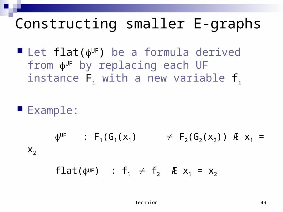
Constructing smaller E-graphs
Let flat(UF) be a formula derived from UF by replacing each UF instance Fi with a new variable fi
Example:
UF : F1(G1(x1) F2(G2(x2)) Æ x1 = x2
flat(UF) : f1 f2 Æ x1 = x2
Technion 50
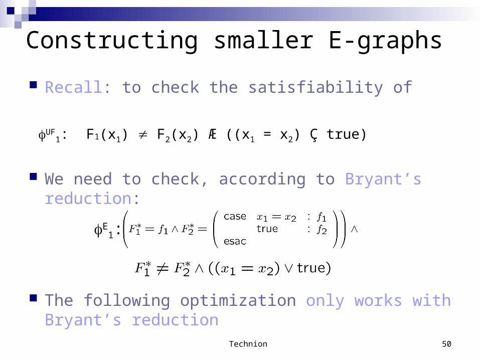
Constructing smaller E-graphs
Recall: to check the satisfiability of
UF1: F1(x1) F2(x2) Æ ((x1 = x2) Ç true)
We need to check, according to Bryant’s reduction:
The following optimization only works with Bryant’s reduction
E1:
Technion 51
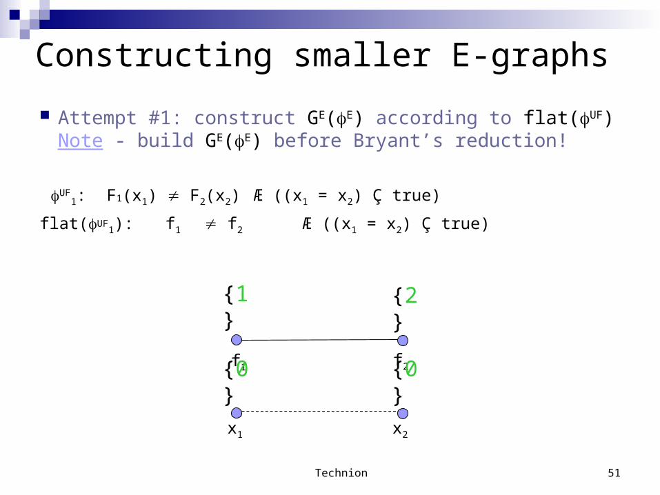
Constructing smaller E-graphs
Attempt #1: construct GE(E) according to flat(UF)Note - build GE(E) before Bryant’s reduction!
UF1: F1(x1) F2(x2) Æ ((x1 = x2) Ç true)
flat(UF1): f1 f2 Æ ((x1 = x2) Ç true)
f1 f2
x2x1
{1} {2}
{0} {0}

Technion 52
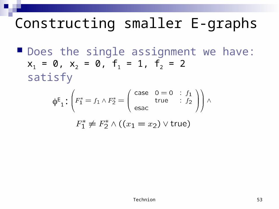
Constructing smaller E-graphs
Does the single assignment we have: x1 = 0, x2 = 0, f1 = 1, f2 = 2
satisfy
E
1:
Technion 53
Constructing smaller E-graphs
Does the single assignment we have: x1 = 0, x2 = 0, f1 = 1, f2 = 2
satisfy
E
1:
Technion 54
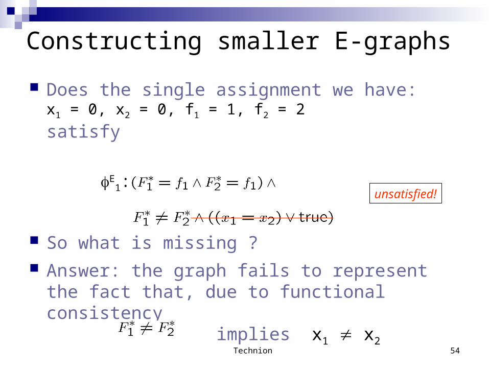
Constructing smaller E-graphs
Does the single assignment we have: x1 = 0, x2 = 0, f1 = 1, f2 = 2
satisfy
So what is missing ? Answer: the graph fails to represent the fact that, due
to functional consistency implies x1 x2
unsatisfied!E
1:
Technion 55
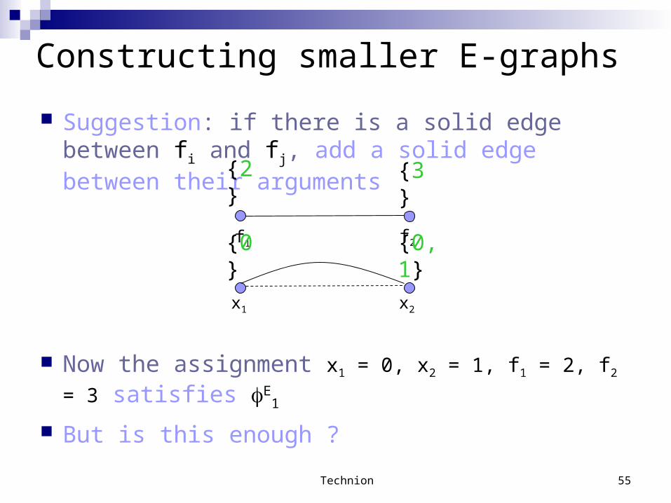
Constructing smaller E-graphs
Suggestion: if there is a solid edge between fi and fj, add a solid edge between their arguments
Now the assignment x1 = 0, x2 = 1, f1 = 2, f2 = 3 satisfies E
1
But is this enough ?
f1 f2
x2x1
{2} {3}
{0} {0,1}
Technion 56
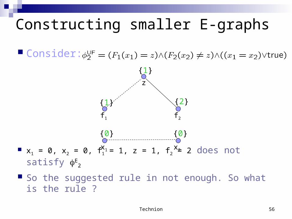
Constructing smaller E-graphs
Consider:
x1 = 0, x2 = 0, f1 = 1, z = 1, f2 = 2 does not satisfy E2
So the suggested rule in not enough. So what is the rule ?
f1 f2
{1} {2}
x2x1
{0} {0}
z
{1}
Technion 57
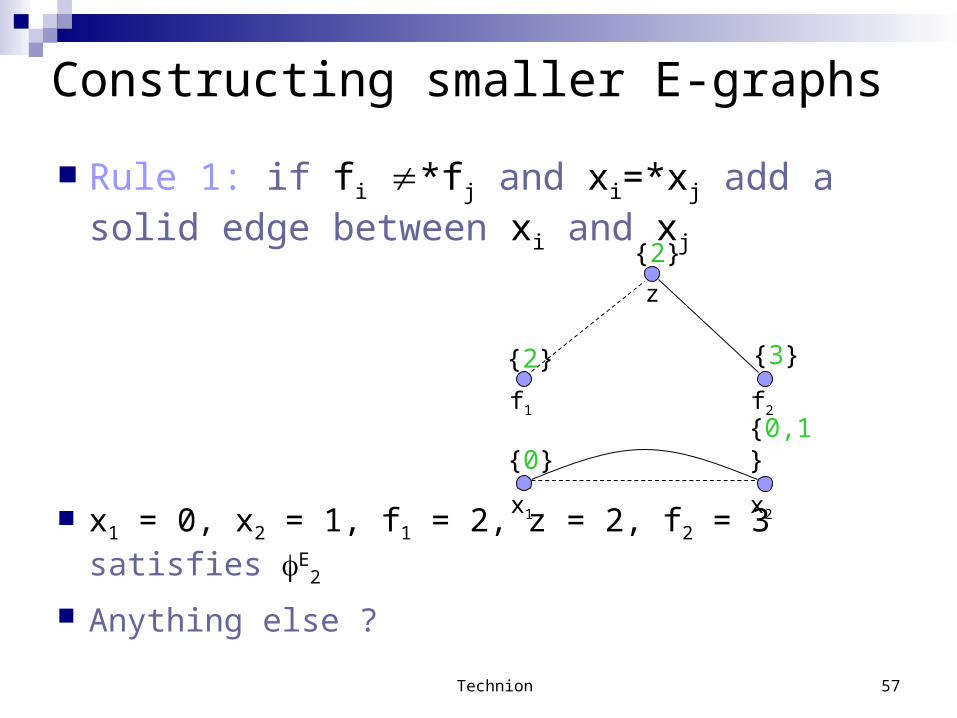
Constructing smaller E-graphs
Rule 1: if fi *fj and xi=*xj add a solid edge between xi and xj
x1 = 0, x2 = 1, f1 = 2, z = 2, f2 = 3 satisfies E2
Anything else ?
f1 f2
x2x1
z
{2} {3}
{0} {0,1}
{2}
Technion 58
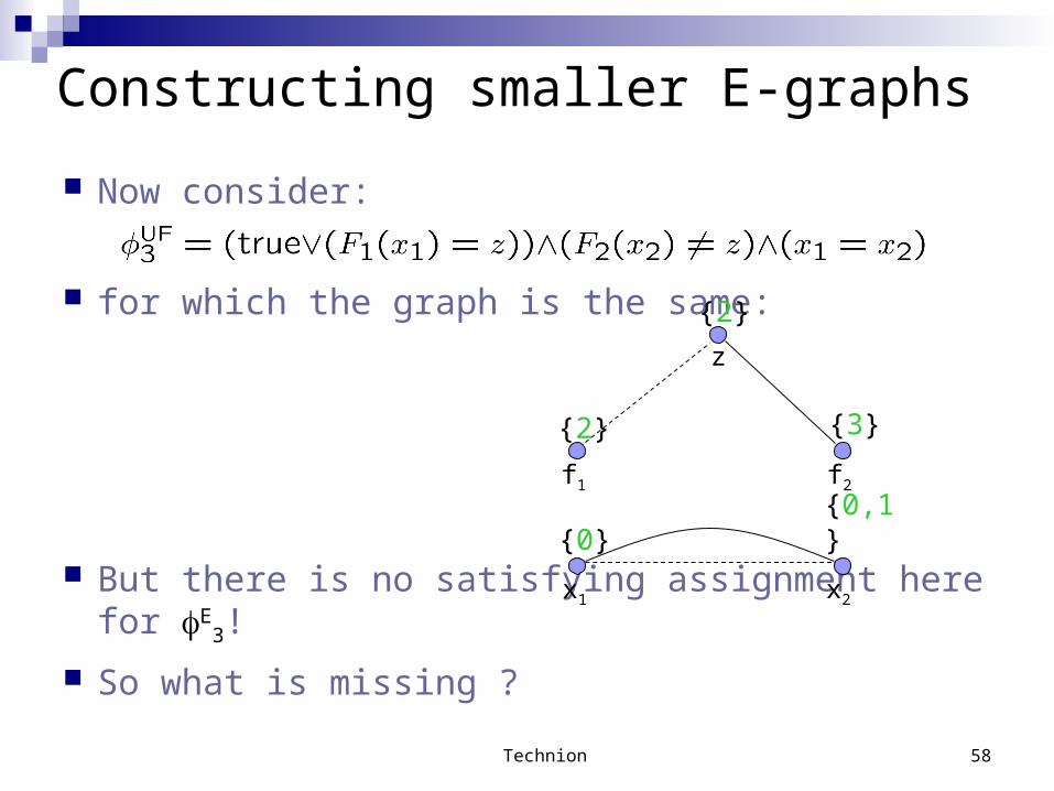
Constructing smaller E-graphs
Now consider:
for which the graph is the same:
But there is no satisfying assignment here for E3!
So what is missing ?
f1 f2
{2} {3}
x2x1
{0} {0,1}
z
{2}
Technion 59
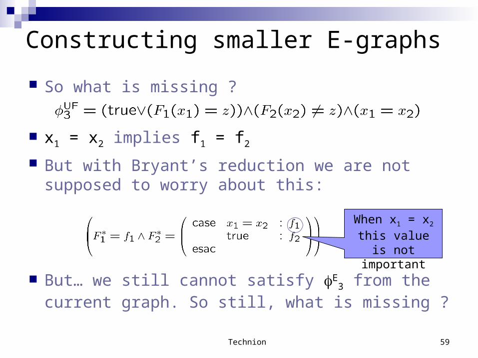
Constructing smaller E-graphs
So what is missing ?
x1 = x2 implies f1 = f2
But with Bryant’s reduction we are not supposed to worry about this:
But… we still cannot satisfy E3 from the current graph.
So still, what is missing ?
When x1 = x2 this value is not important
Technion 60
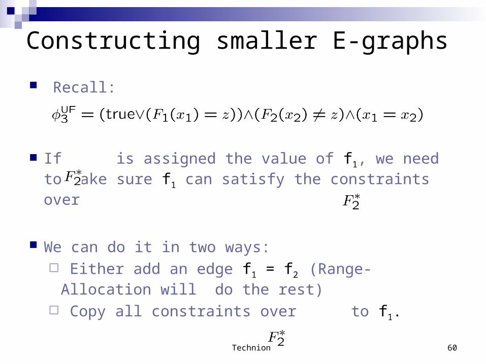
Constructing smaller E-graphs
Recall:
If is assigned the value of f1, we need to make sure f1 can satisfy the constraints over
We can do it in two ways: Either add an edge f1 = f2 (Range-Allocation will do
the rest) Copy all constraints over to f1.
Technion 61
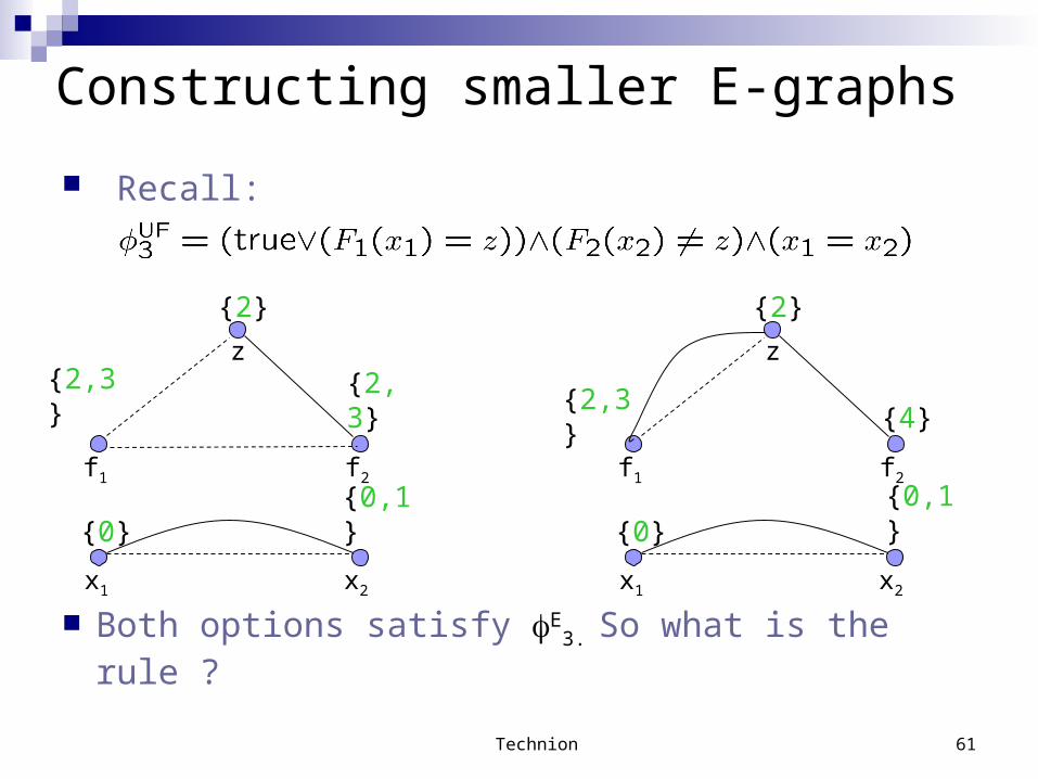
Constructing smaller E-graphs
Recall:
Both options satisfy E3. So what is the rule ?
f1 f2
x2x1
z
{2,3} {2,3}
{0} {0,1}
{2}
f1 f2
x2x1
z
{2,3}{4}
{0} {0,1}
{2}
Technion 62
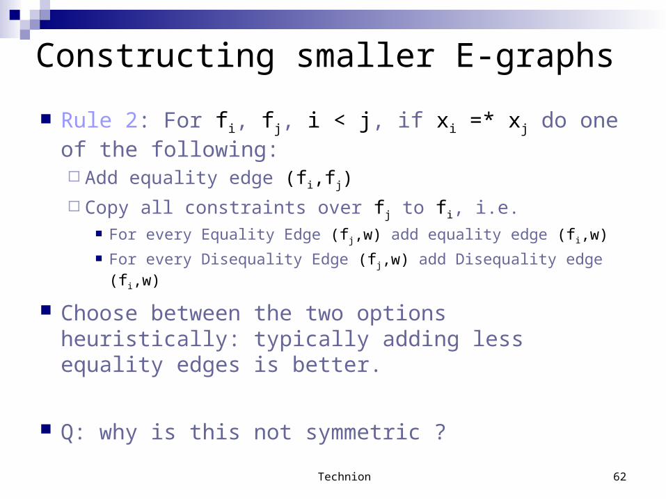
Constructing smaller E-graphs
Rule 2: For fi, fj, i < j, if xi =* xj do one of the following: Add equality edge (fi,fj)
Copy all constraints over fj to fi, i.e. For every Equality Edge (fj,w) add equality edge (fi,w)
For every Disequality Edge (fj,w) add Disequality edge (fi,w)
Choose between the two options heuristically: typically adding less equality edges is better.
Q: why is this not symmetric ?
Technion 63
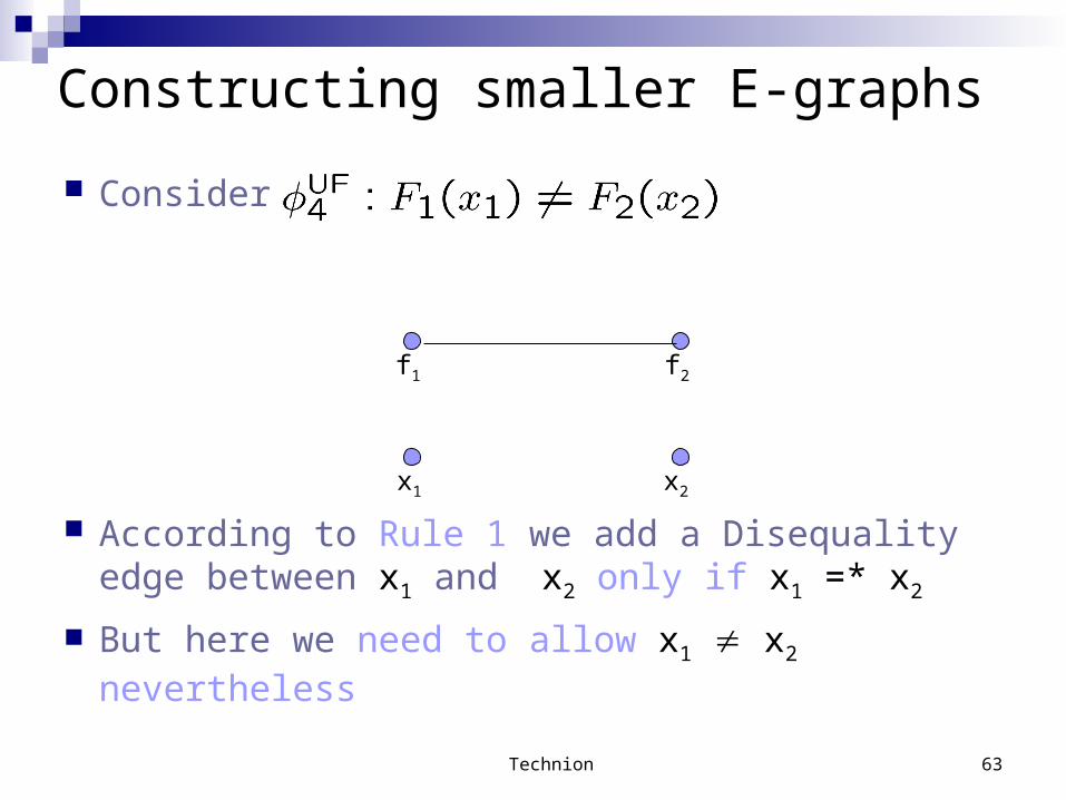
Constructing smaller E-graphs
Consider
According to Rule 1 we add a Disequality edge between x1 and x2 only if x1 =* x2
But here we need to allow x1 x2 nevertheless
f1 f2
x2x1
Technion 64
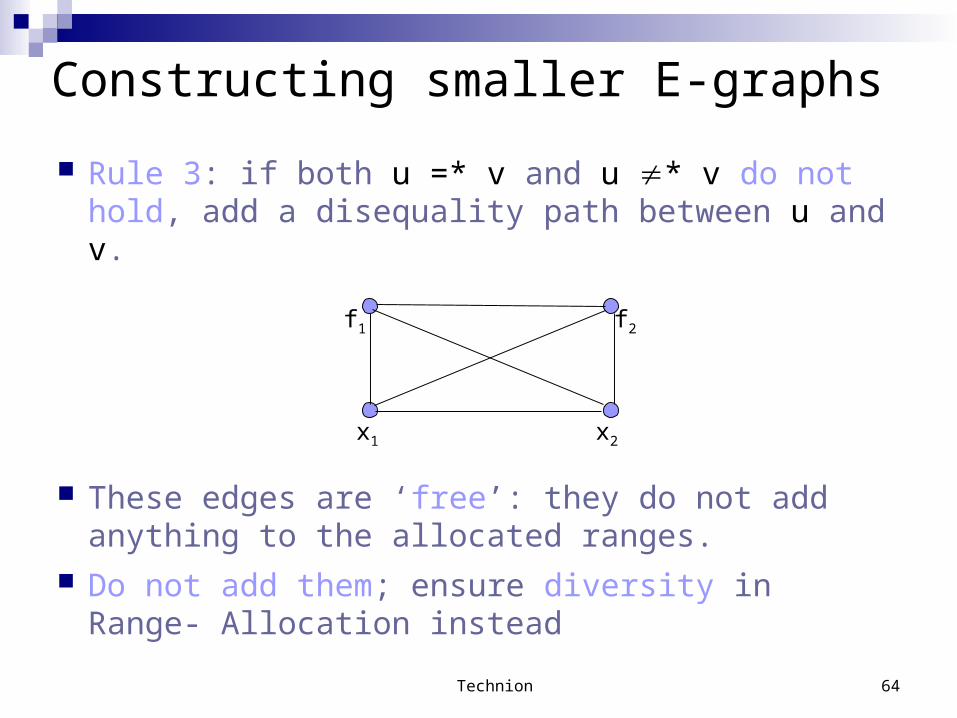
Constructing smaller E-graphs
Rule 3: if both u =* v and u * v do not hold, add a disequality path between u and v.
These edges are ‘free’: they do not add anything to the allocated ranges.
Do not add them; ensure diversity in Range- Allocation instead
f1 f2
x2x1
Technion 65
Constructing smaller E-graphs
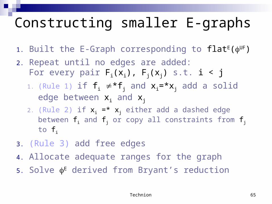
1. Built the E-Graph corresponding to flatE(UF)
2. Repeat until no edges are added:For every pair Fi(xi), Fj(xj) s.t. i < j
1. (Rule 1) if fi *fj and xi=*xj add a solid edge between xi and xj
2. (Rule 2) if xi =* xj either add a dashed edge between fi and fj or copy all constraints from fj to fi
3. (Rule 3) add free edges
4. Allocate adequate ranges for the graph
5. Solve E derived from Bryant’s reduction
Technion 66
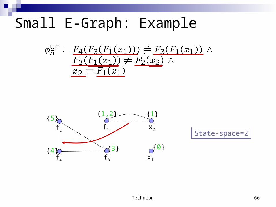
Small E-Graph: Example
f1f2
x1
x2
f3f4
{0}
{1}{1,2}
{3}{4}
{5}
State-space=2
Technion 67
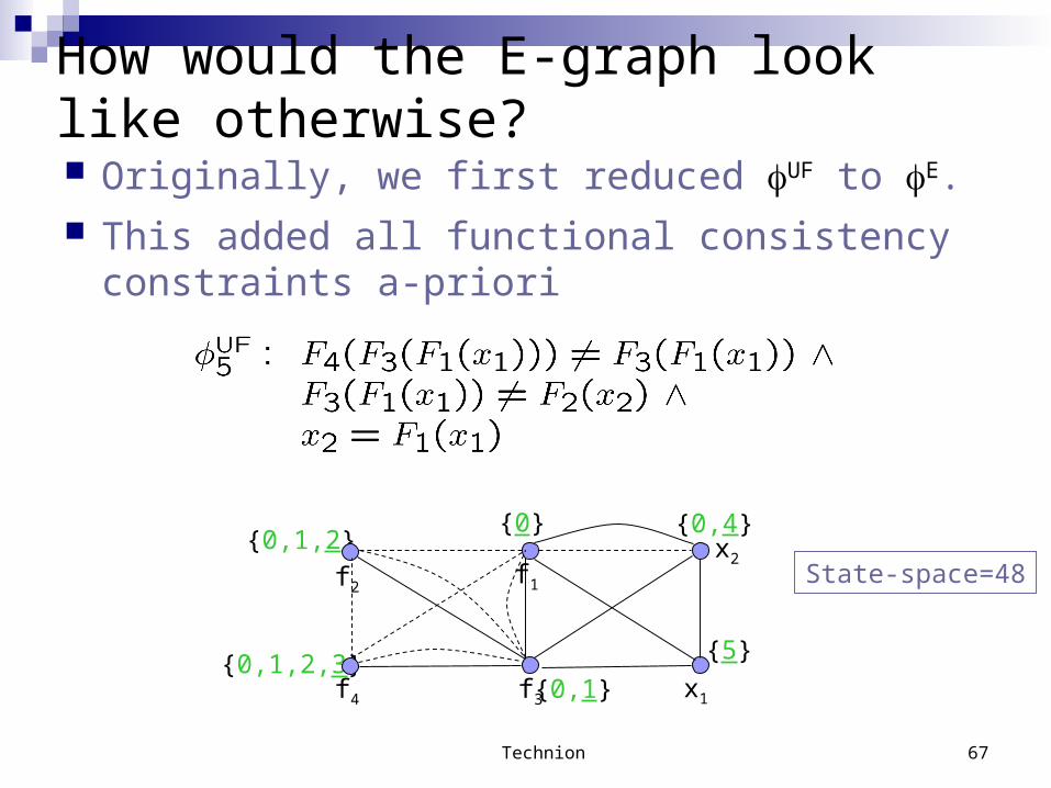
How would the E-graph look like otherwise?
{5}
{0,4}{0}
{0,1}{0,1,2,3}
{0,1,2}f1f2
x1
x2
f3f4
Originally, we first reduced UF to E. This added all functional consistency constraints a-
priori
State-space=48
Technion 68
Bryant’s vs. Ackermann’s reduction
Why only Bryant’s reduction works in this case? The short answer:
Bryant’s: when the arguments are equal, it doesn’t matter if f1 and f2 are equal.
Ackermann’s: giving unique values to f1,f2 makes the formula unsatisfiable when x1 = x2
(x1 = x2 ! f1 = f2) Æ flat(UF)
The long answer: see lecture notes