Embed Size (px)
Citation preview

On Robustness of Motion Control Systems
by
Quang Phuc Ha, B .E. (Ho Chi Minh City) , Ph.D. (Moscow)
Department of Electrical and Electronic Engineering
Submitted in fulfilment of the requirements for the degree of
Doctor of Philosophy
The University of Tasmania
December 1996

To the memory of my mother, Trdn thj Muoi

Statement of Originality
This thesis contains no material which has been accepted for the award of any other
degree or diploma in any tertiary institution. To the best of my knowledge and belief,
the thesis contains no material previously or written by another person, except when
due reference is made in the text.
Quang Phuc Ha
iii

Acknowledgments
Firstly, I would like to thank Dr Michael Negnevitsky for his appreciable guidance
and support as a supervisor. I am particularly grateful to Professor Thong Nguyen,
Head of the Electrical and Electronic Engineering Department at the University of
Tasmania, for his valuable advice and consistent encouragement during my work. I
would also like to thank all the academic staff; John Brodie, Peter Watt, Richard
Langman, Bob Wherrett, Greg The, Dr David Lewis, Dr Habib Talhami, Dr Zhihong
Man, and technical staff; Glenn Mayhew, Russell Twining, David Craig, Steven
A very, Alec Co sic, Bernard Chenery, and especially the departmental secretary, Mrs
Judy Bonsey, for their kind assistance and friendship. Many thanks go to my fellow
postgraduate students, especially Andrew Innes and Richard Andrews for reading
through some of my manuscript papers. I thankfully appreciate financial assistance
from the Department and the Faculty of Engineering while undertaking my study.
Lastly, I would like to extend my thanks and also dedicate this work to my wife,
Nguy�n thi NgQc Hoa, and my father, Ha Thong, for their love, care, and support.
iv

Abstract
Robustness and intelligence are becoming increasingly important in motion control
systems. In multi-mass electromechanical systems, the estimation of damping
capability and design of robust controllers are among very important aspects. In this
thesis, conventional control methods coupled with fuzzy logic and neural networks
are used to address these issues.
First, damping capability of multi-mass electromechanical systems is estimated. The
maximal damping and complete damping cases are determined using the generalised
model for a multi-mass electromechanical system. To eliminate the load variation
influence and reduce elastic vibrations, robust modal control is proposed with
observer-based state feedback and feedforward compensation.
The use of fuzzy logic dealing with uncertainties is investigated. Good transient
performance is obtained, even in the case of changing plant parameters, by fuzzy
tuning of the proportional-integral (PI) controller parameters. It is shown that PI
controllers with fuzzy tuning can be used in cascade control in a two-mass system.
Fuzzy tuning schemes, based on expert knowledge, can be applied to sliding mode
control to accelerate the reaching phase and reduce chattering for robustness
enhancement.
In robust modal control , taking into account uncertainties in the plant parameters and
disturbance rate of change, an improvement of observer robustness is achieved via a
fuzzs tuning scheme of the predictive coefficient. Insensitivity to load variations is
enhanced by continuously tuning the feedforward compensation coefficients. These
fuzzy tuning schemes can be applied to robust modal control of multi-mass systems in
the presence of uncertainties. Since tuning is a continuous process, exponential
membership functions are used. However, with Gaussian or sigmoidal membership
v

Abstract vi
functions, similar results can also be obtained. Observer robustness achieved by fuzzy
tuning is demonstrated to be suitable for incipient fault detection in dynamic systems.
Neural network-based techniques to the problem concerned are also presented. It is
shown that a neural net controller can replace the role of a feedforward controller or a
fuzzy logic controller. Moreover, a neural net-based controller can be used as a
classifier for recognising the error and derivative-of-error patterns, and providing an
appropriate control action to improve tracking performance. The proposed controller
can be used in a two-mass system without a priori knowledge of the plant. Neuro-·
fuzzy approach is introduced with a feedforward compensation from an observer
based control loop and robust enhancement from a neural network model .
Tuning is a human experience to increase robustness. Fuzzy tuning is shown to be
efficient thanks to the possibility of adopting this experience. Neurotuning with
learning capability will be a subject for further research.
vi

Contents
Acknowledgments
Abstract
Contents
Thesis organisation and list of publications
iv
v
vii
X
1. Introduction 1
1 . 1 Robust control . . . . . . . . . . . . . . . . . . . . . . . . . . . . . . . . . . . . . . . . . . . . . . . . . 1
1 .2 Intelligent control . . . . . . . . . . . . . . . . . . . . . . . . . . . . . . . . . . . . . . . . . . . . . . . 2
1 .3 Robustness via fuzzy tuning . . . . . . . . . . . . . . . . . . . . . . . . . . . . . . . . . . . . . . . 3
1 .4 Neural network application for control performance enhancement. . . . . . . . . . 4
1 .5 Thesis contributions . . . . . . . . . . . . . . . . . . . . . . . . . . . . . . . . . . . . . . . . . . . . . 5
2. Multi-mass electromechanical systems: damping capability estimation 7
2 . 1 Introduction . . . . . . . . . . . . . . . . . . . . . . . . . . . . . . . . . . . . . . . . . . . . . . . . . . . . 7
2.2 Generalised model for a multi-mass electromechanical system . . . . . . . . . . . . 8
2.3 EMS characteristic equation in dimensionless space . . . . . . . . . . . . . . . . . . . 1 1
2.4 Maximal damping conditions . . . . . . . . . . . . . . . . . . . . . . . . . . . . . . . . . . . . . 1 6
2.5 Root loci of multi-mass electromechanical systems . . . . . . . . . . . . . . . . . . . . 20
2.6 Viscous friction influence . . . . . . . . . . . . . . . . . . . . . . . . . . . . . . . . . . . . . . . . 3 1
2.7 Illustrative examples . . . . . . . . . . . . . . . . . . . . . . . . . . . . . . . . . . . . . . . . . . . . 35
2 .8 Summary . . . . . . . . . . . . . . . . . . . . . . . . . . . . . . . . . . . . . . . . . . . . . . . . . . . . . 37
3. Robust modal control: an overview 39
3 . 1 Introduction . . . . . . . . . . . . . . . . . . . . . . . . . . . . . . . . . . . . . . . . . . . . . . . . . . . 39
3.2 Modal control . . . . . . . . . . . . . . . . . . . . . . . . . . . . . . . . . . . . . . . . . . . . . . . . . 40
3 .3 Dominant pole-based assignment and sensitivity analysis . . . . . . . . . . . . . . . 50
3 .4 Combined observer for state and disturbance estimation . . . . . . . . . . . . . . . . 62
Vll

Contents viii
3 .5 Observer-based feedforward compensation . . . . . . . . . . . . . . . . . . . . . . . . . . 7 1
3 .6 Robust modal control . . . . . . . . . . . . . . . . . . . . . . . . . . . . . . . . . . . . . . . . . . . 75
3. 7 Summary . . . . . . . . . . . . . . . . . . . . . . . . . . . . . . . . . . . . . . . . . . . . . . . . . . . . . 84
4. Fuzzy logic and fuzzy logic controller 86
4 . 1 Introduction . . . . . . . . . . . . . . . . . . . . . . . . . . . . . . . . . . . . . . . . . . . . . . . . . . . 86
4.2 Fuzzy set theory . . . . . . . . . . . . . . . . . . . . . . . . . . . . . . . . . . . . . . . . . . . . . . . . 88
4.3 Fuzzy logic and fuzzy reasoning . . . . . . . . . . . . . . . . . . . . . . . . . . . . . . . . . . . 96
4.4 Fuzzy logic control . . . . . . . . . . . . . . . . . . . . . . . . . . . . . . . . . . . . . . . . . . . . 10 1
4 .5 Fuzzy control : pros, cons, and perspective . . . . . . . . . . . . . . . . . . . . . . . . . . 1 25
4.6 Summary . . . . . . . . . . . . . . . . . . . . . . . . . . . . . . . . . . . . . . . . . . . . . . . . . . . . 1 27
5. Robustness enhancement with fuzzy tuning 128
5. 1 Introduction . . . . . . . . . . . . . . . . . . . . . . . . . . . . . . . . . . . . . . . . . . . . . . . . . . 1 28
5.2 Fuzzy tuning in PI controllers . . . . . . . . . . . . . . . . . . . . . . . . . . . . . . . . . . . . 1 30
5 .3 Cascade PI controllers with fuzzy tuning . . . . . . . . . . . . . . . . . . . . . . . . . . . 1 37
5.4 Sliding mode controller with fuzzy tuning . . . . . . . . . . . . . . . . . . . . . . . . . . 144
5 .5 Summary and further discussion . . . . . . . . . . . . . . . . . . . . . . . . . . . . . . . . . . 15 1
6 . Robust modal control with fuzzy tuning 157
6 . 1 Introduction . . . . . . . . . . . .. . . . . . . . . . . . . . . . . . . . . .. . . . . . . .. . . . . . . . 1 57
6.2 Digital predictive observer with fuzzy tuning . . . . . . . . . . . . . . . . . . . . . . . . 1 58
6.3 Feedforward controller with fuzzy tuning . . . . . . . . . . . . . . . . . . . . . . . . . . . 1 65
6.4 Modal controller with fuzzy tuning . . . . . . . . . . . . . . . . . . . . . . . . . . . . . . . . 177
6.5 Fuzzy tuning w ith different membership functions . . . . . . . . . . . . . . . . . . . 1 86
6.6 Summary . . . . . . . . . . . . . . . . . . . . . . . . . . . . . . . . . . . . . . . . . . . . . . . . . . . . 1 9 1
7 . Neural network application to motion control 193
7. 1 Introduction . . . . . . . . . . . . . . . . . . . . . . . . . . . . . . . . . . . . . . . . . . . . . . . . . . 193
7 .2 Neural networks for control systems . . . . . . . . . . . . . . . . . . . . . . . . . . . . . . . 195
7.3 Neural network implementation of a fuzzy logic controller . . . . . . . . . . . . . 206
7.4 Neural network-based controller for tracking systems . . . . . . . . . . . . . . . . . 2 1 1
viii

Contents ix
7.5 Robust control u sing neuro-fuzzy approach . . . . . . . . . . . . . . . . . . . . . . . . . 226
7 .6 Summary and discussion . . . . . . . . . . . . . . . . . . . . . . . . . . . . . . . . . . . . . . . . 237
8. Summary and future extensions 240
8 . 1 Introduction . . . . . . . . . . . . . . . . . . . . . . . . . . . . . . . . . . . . . . . . . . . . . . . . . . 240
8 .2 Summary of results . . . . . . . . . . . . . . . . . . . . . . . . . . . . . . . . . . . . . . . . . . . . 241
8 .3 Further extensions and developments . . . . . . . . . . . . . . . . . . . . . . . . . . . . . . 245
8 .4 Concluding remarks . . . . . . . . . . . . . . . . . . . . . . . . . . . . . . . . . . . . . . . . . . . 247
A. Normalised closed-loop polynomials
B. A digital predictive observer for incipient fault detection
References
ix
249
250
258

Thesis Organisation and List of Publications
Thesis Organisation
This thesis is organised into eight chapters . The first chapter introduces the aim of this
work, recent strategies to achieve robust enhancement in motion control systems, and
its contributions to the topic. Chapter 2 is devoted to the estimation of damping
capability of multi-mass electromechanical systems, considering also the influence of
varying electro-magnetic and electromechanical time-constants, and of viscous
friction. Chapter 3 is involved in the robust modal control technique covering the
design of a combined observer for the states and disturbances, a feedforward
controller, and a robust controller. Chapter 4 outlines primary concepts of fuzzy logic
and fuzzy logic control and illustrates the design of a fuzzy logic controller for an
overhead crane model . Chapter 5 is concerned with the use of fuzzy logic to tune the
controller parameters in proportional-integral control and the control action in sliding
mode control. Chapter 6 applies fuzzy tuning schemes resulting in explicit
expressions to adjust the robust modal control parameters for improving system
robustness. Chapter 7 employs the ability of a neural network to approximate an
input/output relation, to classify the patterns of error and its derivative, and to learn
the inverse dynamics for robust enhancements in motion control systems. Finally,
Chapter 8 provides a summary of main results of this thesis and suggests some
avenues for future research.
Supporting Publications
This research resulted in a number of journal and conference papers listed below:
1. Journal papers: [ 1] Ha, Q.P., "A robust sliding mode controller with fuzzy tuning," lEE Electronics
Letters, Vol. 32, No. 17 , pp. 1 626- 1 628, August 1 996.
X

Thesis organisation and list of publications xi
[2] Ha, Q.P. , "PI controllers with fuzzy tuning," lEE Electronics Letters" Vol. 32,
No. 1 1 , pp. 1043- 1 044, May 1 996.
[3] Ha, Q.P. and Negnevitsky, M., "Robust controllers with fuzzy tuning" ,
Australian Journal of Intelligent Information Processing Systems, Vol. 3 , No 3 ,
pp . 33-40, 1 996.
[4] Alferov, V.G. and Ha, Q.P. , "A digital observer device with prediction, "
Elektromekhanika, No 3 , pp. 7 1 -76, March 1 992. In Russian.
English abstract in INSPEC no. 431647, Institution of Electrical Engineers.
[5] Alferov, V.G. and Ha, Q.P., "Using the root-locus method and dominant root
pairs for dynamic properties estimation, " Elektrotekhnika, No 6, pp. 29-32, June
1 993. In Russian.
English abstract in COMPENDEX no.378346, Engineering Info. Inc.
English translation by Allerton Press, Inc.: Soviet Electrical Engineering, 1993, No 6, pp. 35-40.
[6] Alferov, V.G. and Ha, Q.P. , "Design of a modal control system for servo drive,"
Elektrichestvo, No 6, pp. 48-54, June 1 993 . In Russian.
English abstract in IN SPEC no. 4515187, Institution of Electrical Engineers.
[7] Alferov, V.G. and Ha, Q.P. , "DC-motor position drives with robust modal
control, " Elektrichestvo, No 9, pp. 17-24, September 1995. In Russian.
English abstract in IN SPEC no. 5140507, Institution of Electrical Engineers.
[8] Ha, Q.P. and Alferov, V.G., "On the problem of parameter sensitivity in control
system of DC motor position drive," Elektrichestvo, No. 1 , pp. 47-53, January
1 996. In Russian.
2. Chapter in a book: [9] Ha, Q.P. and Negnevitsky, M. , "Fuzzy tuning in motion control" , in
Applications of Art{ficial Intelligence in Engineering XI, Computational
Mechanics Publications, R.A. Adey, G. Rzevski, and A K. Sunol (Eds. ),
Southampton, UK, 1 996, 734p.
3. Refereed international conference papers: [ 1 0] Ha, Q.P. and Negnevitsky, M. , "Neural network-based controller for servo
drives, " in Proceedings of the IEEE 22nd International Conference on
xi

Thesis organisation and list of publications xii
Industrial Electronics, Control, and Instrumentation (IECON 96), Taipei,
Taiwan, Vol . 2, pp. 904-909, August 1 996.
[ 1 1 ] Palis, F., Buch, A., Ladra U., Kurrich R., Ha, Q.P., and Negnevitsky, M. ,
"Robust control using neuro-fuzzy approach" , in Proceedings of the
International Conference on Electrical Drives and Power Electronics (EDPE
96), Kosice, Slovakia, Vol. 1 , pp. 1 94- 1 98, October 1 996.
[ 1 2] Ha, Q.P. , Negnevitsky, M. and Man, Z., "Sliding mode control with fuzzy
tuning" , in Proceedings of the IEEE 4th Australian and New Zealand
Conference on Intelligent Information Systems (ANZIIS 96), Adelaide,
Australia, pp. 2 1 6 -219 , October 1 996.
[ 1 3] Palis, F., Buch, A . , Ladra U., Kurrich R., Ha, Q.P., and Negnevitsky, M.,"Fuzzy
and neurocontrol of drive systems with changing parameters and load" , in
Proceedings of the European Power Electronics Symposium on Electric Drive
Design and Applications (EPE 96), Nancy, France, pp. 1 83- 186, June 1996.
[ 1 4] Ha, Q.P. and Negnevitsky, M., "Neural network application for the position
drive of a swinging load" , in Proceedings of the International Conference on
Modelling, Simulation and Optimization (lASTED 96), Gold Coast, Australia,
May 1 996.
[ 1 5] Ha, Q.P. and Negnevitsky, M. , "Fuzzy tuning in robust modal control, " in
Proceedings of the 1st International Discourse on Fuzzy Logic and the
Management of Complexity (FLAMOC 96), Sydney, Australia, Vol. 2, pp. 1 60-
1 64, January 1 996 .
[ 1 6] Negnevitsky, M. , Ha, Q.P. , L.P. Chee and T.H. Ting, "A fuzzy logic controller
for an overhead crane", in Proceedings of the 1st International Discourse on
Fuzzy Logic and the Management of Complexity (FLAMOC 96), Sydney,
Australia, Vol . 2 , pp. 1 7 1 - 175, January 1 996.
[ 1 7] Ha, Q.P. and Negnevitsky, M. , "Root locus application for damping capability
estimation of multi-mass electromechanical systems," in Proceedings of the
IEEE 21st International Conference on Industrial Electronics, Control, and
Instrumentation (IECON 95), Orlando, USA, vol. 1 , pp. 633-638, November
1 995 .
[ 1 8] Ha, Q.P. and Negnevitsky, M. , "A digital predictive observer for incipient fault
detection, " in Proceedings of the lEE 3rd International Conference on
X11

Thesis organisation and list of publications xiii
Advances in Power System, Operation & Management (APSCOM 95),
HongKong, vol . 1 , pp. 1 83-1 88, November 1 995.
[ I 9] Ha, Q.P. and Negnevitsky, M., "A robust modal controller with fuzzy tuning for
multi-mass electromechanical systems," in Proceedings of the IEEE 3rd
Australian and New Zealand Conference on Intelligent Information Systems
(ANZIIS 95), Perth, Australia, pp. 2 14-2 19, November 1 995.
[20] Ha, Q.P. and Negnevitsky, M., "New trends in control theory and their
reflection in electrical engineering education," in Proceedings of the Pacif1c
Region Conference on Electrical Engineering Education (PRCEEE 95),
Victoria, Australia , pp. 1 09- 1 12, February 1 995.
[2 1 ] Ha, Q.P. , Negnevitsky, M. , and Palis, F., "Cascade PI controllers with fuzzy
tuning" , to appear in Proceedings of the 6th IEEE International Conference on
Fuzzy Systems (FUZZ-IEEE 97), Barcelona, Spain, July 1 997 .
[22] Ha, Q.P. , Negnevitsky, M. and Man, Z., "Dominant pole-based controller for
maximal damping of multi-mass systems" , to appear in Proceedings of the 2nd
Asian Control Conference (ASCC 97), Seoul, Korea, July 1 997 .
[23] Man, Z. , Yu, X. H. , and Ha, Q.P. , "Adaptive control using fuzzy basis function
expansion for SISO linearisable nonlinear systems" , to appear in Proceedings of
the 2nd Asian Control Conference (ASCC 97), Seoul, Korea, July 1997.
[24] Man, Z., Yu, X.H. , and Ha, Q.P. , "A study of uncertainty bound for rigid robot
control systems", to appear in Proceedings of the 2nd Asian Control Conference
(ASCC 97), Seoul , Korea, July 1 997.
[25] Ha, Q.P. and Negnevitsky, M., "Continuous variable structure systems with
fuzzy tuning" , submitted to the 5th IEEE Australian and New Zealand
Conference on Intelligent Information Systems ANZIIS'97 , Dunedin, New
Zealand, November 1 997.
4. Refereed national conference papers: [26] Ha, Q.P. , "A neural network-based controller for multi-mass electromechanical
systems, " in Proceedings of the Australian Universities Power Engineering
Conference (AUPEC 96), Melbourne, Australia, Vol. 1 , pp. 3 1 -36, October
1996.
xiii

Thesis organisation and list ofpublications xiv
[27] Ha, Q.P., "Root locus method application for damping capability estimation of
multi-mass electromechanical systems," in Preprints of the CONTROL'95
Conference, Melbourne, Australia, vol . 1 , pp. 255-259, October 1995.
[28] Ha, Q.P. and Pal is , F. , "Fuzzy logic application in a robust modal controller for
position drives," in Proceedings of the 30th Universities Power Engineering
Conference (UPEC 95), London, UK, vol. l , pp. 85-89, September 1 995.
[29] Ha, Q.P., "A digital predictive observer with fuzzy tuning for multi-mass
electromechanical systems, " in Proceedings of the Australian Universities
Power Engineering Conference (AUPEC 95), Perth, Australia, vol. 3 , pp. 422-
427, Septemberl 995.
[30] Ha, Q.P., "A dynamic feedforward controller with fuzzy tuning for
electromechanical systems," in Proceedings of the Australian Universities
Power Engineering Conference (AUPEC 95), Perth, Australia, vol. 3 , pp. 428-
433, September 1 995.
[3 1 ] Ha, Q.P. and Alferov, V.G., "Robust modal controller for position drives," in
Preprints. of the Electrical Engineering Congress (EEC 94), Sydney, Australia,
pp. 609-6 14, November 1 994.
[32] Alferov, V.G., Ha, Q.P. , and Khusainov, R.M., "Drive control systems with a
disturbance observer, " in Industrial application. of electric drives on the
perspective element base, N.F. Ilynsky (Ed.), Moscow, Russia, pp. 93-99, May
1 992. In Russian.
xiv

Chapter 1
Introduction
The emergency of motion control field started since 1 970's through the application of
control theory to power electronics by the use of microprocessors to drive electrical
motors . Motion control is currently accepted as an established and prominent field of
technology covering control engineering, computer science and mechanical
engineering (Harashima [ 1 ] ) . Two main issues in motion control systems are
robustness against parameter variations and disturbances, and the intelligent capability
to adjust the control system itself to environment changes and task requirements. This
thesis is an attempt to combine conventional methods and recently developed
techniques, namely fuzzy logic and neural network, to address the problem of
robustness enhancement in electromechanical systems or, in general, dynamic
systems. Towards that aim some control strategies are involved as follows.
1.1 Robust Control
Robustness is the property of a dynamic system being insensitive to significant plant
uncertainties. Dorato in [2] noted that although solutions to this classical control
problem have been proposed for a long time, the actual term "robust control" first
appeared in a conference paper by Davidson in 1 973. Robust controllers have been
explored extensively in literature in the last two decades (Dorato et al. [3] , Tsypkin
[4] ) . Robust control has been widely applied to enhance performance of dynamic
systems subject to any sources of uncertainty and changing environments . Various
methods of modern control theory have been developed for the analysis and design of
these systems. In addition to impressive progress in the theory and applications of

Chapter 1. Introduction 2
optimal control and adaptive control, since the middle of 1 970's intensive efforts have
been dedicated to robust control which deals with the design of fixed controllers .
Robust stability of dynamic systems has been of interest since the seminal paper by
Kharitonov [5]. The most popular in robust control is the H-infinity method,
originated by Zames in 1979, based on frequency optimisation (Kwakernaak [6]). The
variable structure system with sliding-mode method, first introduced by Emelyanov
[7] and then developed by Utkin [8] , is also effective for robust control . Robust
control methods are now useful for applications because of the prolific computational
resources for implementing control algorithms and associated electronic devices. As
an application to electromechanical systems, robust modal control proposed by Ha
[9], a state feedback method, is under investigation in this thesis. Moreover, with a
partially known environment some artificial intelligent tools are incorporated to the
control system to improve robustness .
1.2 Intelligent control
Qualitatively, a system which includes the ability to sense its environment, process the
information to reduce uncertainty, and generate and execute control action for several
situations constitutes an intelligent control system (Kumar & Mani [ 10]) . Advances in
the areas of artificial intelligence have demonstrated a potential for new approaches to
the control of complex systems under changing environments and performance
criteria, unmeasurable disturbances and component failure. Artificial intelligence
tools, such as expert system, fuzzy logic, and neural network are expected to usher a
new area in motion control in the coming decades. In the early 1 970's a way of
structuring software that closely matches the human thinking process, called "expert
system" was born and has found wide applications in many areas (Bose [ 1 1 ] ) . In a
real-time expert system-based control the input signals, accessed from the sensors, are
processed and control signals for the system are generated. As to "fuzzy logic" , since
the seminal paper by Zadeh on fuzzy sets in 1 965 [ 1 2] , fuzzy systems have developed
explosively, attracting many researchers from around the world. One of the landmark
in this development is the genesis of fuzzy logic control in 1 972 (Chang & Zadeh
[ 1 3]) . The key principle underlying fuzzy logic control is based on a logical model
which represents the thinking process that an operator might go through to control the
system manually . Fuzzy logic control can be considered as one of the intelligent
techniques where engineering is reflected in the controllers. The viability of fuzzy
logic control has been demonstrated through widespread applications (Schwartz et al.

Chapter 1 . Introduction 3
[ 1 4]) . On the other hand, much attention was recently focused on a new branch of
artificial intelligence, called artificial neural network or "neural network. " The
artificial neural network tends to simulate the biological neural network by electronic
computation circuits. The neural network technology was gradually evolving since the
1 950's but only since the beginning of the 1990's has this artificial intelligence tool
captivated the attention of practically the whole scientific community (Widrow & Lehr [ 1 5]) . Indeed, its field of applications is covering process control, diagnostics,
identification, character recognition, robot vision, flight scheduling, etc. (Bose [ 1 1 ]) .
As new trends in control theory, these artificial intell igence tools have found their way
into tertiary institutions for engineering education (Ha & Negnevitsky [ 16]) and are
believed to touch almost every engineering application by the early next century. In
this thesis, fuzzy logic and neural network are used for the purpose of tuning the
controller parameters or providing an appropriate control action through a learning
process to improve robustness and tracking performance of servo systems.
1.3 Robustness via Fuzzy Tuning
Controller parameter tuning is a popular engineering experience. Human skill is
normally utilised to tune the controller parameters to achieve required control
performances. In the design of a knowledge-based feedback controller it is desirable
to embed the expert skill of the designers so that the controller can make decisions on
the choice of appropriate control algorithm. Till now, the proportional-integral
derivative (PID) controllers have been the most popular in industry. For these
controllers, autotuners, which include methods of extracting process dynamics from
experiments and control design methods, have been commercially available since
1 98 1 (Astrom et al. [ 17]) . The application of auto-tuning formulae has brought
intelligent insights into the conventional controllers. In the field of electrical drives,
proportional-integral (PI) controllers with the auto-calibration method, inspired by the
symmetric optimum principles, can be used to tune the controller parameters (Voda & Landau [ 1 8]) . Based on a point of the plant frequency characteristics, autotuning or
auto-calibration of controller parameters in the presence of uncertainties is effective
provided that there is knowledge of the process involved. Truly effective autotuning
schemes for conventional controllers, in general , are restricted to a linear process or a
class of nonlinear process with the presumed range of operation. Using the state space
technique, a robust modal controller (Ha & Alferov [ 1 9]) with fixed parameters
cannot cope well with a large range of uncertainty or nonlinear dynamics. In order to

Chapter 1 . Introduction 4
account for sensor noise, model uncertainties, and severe nonlinearity, the linguistic
characteristics of fuzzy logic with some engineering heuristics provide a good
approach to the uncertainty problem (Tseng & Hwang [20]). In this thesis, tuning the
conventional controllers is accomplished through fuzzy approximate reasoning
techniques with some tuning schemes applied for continuously changing the
coefficients of a cascaded PI controller, a digital predictive observer, a dynamic
feedforward controller, and a robust modal controller (Ha & Negnevitsky [2 1 ] ) , or
changing the control action in a sliding mode controller (Ha et al. [22]) .
1.4 Neural Network Application for Control Performance Enhancement
In recent years there has been a growing interest in applying artificial neural networks
to dynamic systems identification, prediction and control. The use of neural networks
is characterised by the capability of learning from examples or patterns. Thus, it
enables, through a training process, modelling and predicting the behaviour of
complex systems, and providing an appropriate control action to achieve desired
performance, without a priori information about the systems' structures or parameters .
Neural network approaches can be used to a variety of applications in identification,
prediction and control systems (Pham & Xing [23 ]) . The advantages of a neural
network controller over a conventional one are that (i) a much larger amount of
sensory information can be efficiently used in planning and executing a control action,
(ii) the collective processing ability to respond more quickly to complex sensory
inputs, and the most important, (iii) a good adaptation can be achieved through
learning (Psaltis et a l. [24]) . Altnost all the neural network controllers could be
regarded as inverse controllers as they are all based on modelling the inverse
dynamics of the plant. The well-established structures for neural network controllers
using an inverse model are supervised control (Werbos [25]), direct inverse control
(Miller et al. [26]) , model reference control (Narenda & Parthasarathy [27]) , and
internal model control (Hunt & Sbarbaro [28]). In addition to these inverse model
based controllers, there are also other neural controllers originating from conventional
approaches, for example, those based on variable structure technique (Colina-Morles
& Mort [29]) , the robust control strategy (Rovithakis & Christodoulou [30]), the
model predictive method (Evans et al. [3 1 ]), and the parallel adaptive PID-like
controller (Lee et al. [32]) . In this thesis a neural network approach is used for
improving robust performance of motion control systems on the basis of an observer
based controller (Palis, Ha et al. [33]) . Another neural network-based controller is

Chapter I. Introduction 5
proposed here for not modelling the system inverse dynamics but classifying the
patterns of the control error and its derivative, and correspondingly, providing an
appropriate control action to achieve a good tracking performance (Ha & Negnevitsky
[34]).
1.5 Thesis contributions
Throughout this thesis, issues relating to robustness of motion control systems are
addressed. First, the estimation of damping capability of multi-mass
electromechanical systems is addressed. The critical values of the mass ratio are
found. The cases of maximal damping and complete damping are determined. The
influence of parameter variations and viscous friction is investigated by using multi
parameter root loci . It is shown in Ha & Negnevitsky [35] that damping capability is
more affected by variations in viscous friction on the load shaft than on the motor
shaft. For a design procedure to eliminate the load variation influence and reduce
elastic vibrations a robust modal controller is proposed by Ha & Alferov [20], [36]
with feedback signals from the system states and observer-based feedforward
compensation form the disturbance estimate. The use of fuzzy logic as a powerful tool
dealing with uncertainties is investigated through explicit expressions of fuzzy tuning
schemes. The reference response is well-damped with adequately fast dynamics and
the maximum deviation of the disturbance response is reduced, even in the case of
changing plant parameters, by using a fuzzy tuning scheme for conventional PI
controllers (Ha & Negnevitsky [37]) . It is shown in Ha et al. [38] that PI controllers
with fuzzy tuning can be used with cascade control principles in multi-mass systems.
Taking into account uncertainties in the plant parameters and unknown input rate of
change, an improvement of observer robustness is achieved via a fuzzy tuning scheme
of the predictive coefficient (Ha [39]) . Insensitivity to load variations is enhanced
with the dynamic feedforward compensation coefficients continuously tuned by fuzzy
logic (Ha [ 40]) . These fuzzy tuning schemes can be applied to robust modal control
(Ha & Negnevitsky [4 1 ]) or sliding mode control (Ha et al. [22]) of multi-mass
electromechanical systems for vibration suppression and load rejection in the presence
of plant parameter and load uncertainties . Since tuning is a continuous process
exponential membership functions are used. However, with Gaussian or sigmoidal
membership functions, similar results can also be obtained, as reported in Ha & Negnevitsky [42] . Robustness achieved through a fuzzy tuning scheme for an
unknown input observer is demonstrated to be suitable for incipient fault detection in

Chapter 1. Introduction 6 -----------------------------------·
power system, eg. in a synchronous generator (Ha & Negnevitsky [43]) . Neural
network approaches to the problems involved are preliminarily presented at the
closing of the thesis . It is shown that the a neural network can replace the role of a
feedforward controller in Palis, Ha et al. [33] or a fuzzy logic controller in Ha & Negnevitsky [34]. In addition, a neural net-based controller can be used as an
classifier for recognising the control error and derivative-of-error patterns and
providing an appropriate control action to improve tracking performance (Ha & Negnevitsky [44]). The proposed controller can be used in a multi-mass system
without a priori knowledge of the controlled plant (Ha [45]) . For further investigation,
a neuro-fuzzy technique might be a solution to the problem of extracting from the
error signal all the necessary information for a high quality control strategy regardless
of the plant structure and changing environments . It is believed that an architecture for
neurotuning may bring intelligent features into the tuning process and thus, make
dynamic systems cope well with any uncertain factors or severe nonlinearity. Tuning
is a human experience to increase robustness. Fuzzy tuning is shown to be efficient
thanks to the capability of adopting this experience. Neurotuning may be a subject for
further research.
Chapter 2
Multi ... Mass Electromechanical Systems:
Damping Capability Estimation
In industrial applications, many electromechanical systems can be modelled as
consisting of a motor and a load connected with a flexible shaft. A multi-mass system,
in practice, can be the model of a rolling mill, a flexible link arm, a large-scale space
structure, a launch vehicle during the ascent phase, an automobile wheel steering
system, or a mass-spring-damper system, in general. Damping analysis and torsional
oscillation suppression in an electromechanical system (EMS) are classical problems.
However, control issues of flexible structures have gained increasing attention,
especially in space technology where recent efforts are required to maintain high
precision positioning of ever lighter and more flexible structures (Gawronski [46]),
and in robotics where the control of multi-inertia manipulators will be an important
problem in the future of motion control (Lin [47]). Thus, the analysis and design of
these systems are timely and worth being investigated. The thesis starts with the
estimation of damping capability of electromechanical systems served as the common
plant for some controller design procedures discussed in the following chapters .
2.1 Introduction
Special interest has recently been paid to EMS damping capability (see, e.g. , Klepikov
& Samarskii [ 48], Alferov & Ha [ 49] , and Dhaouadi et al. [50]) . In some industrial
applications torsional loads on electrical drive systems may cause undesirable
vibrational effects and lower the dynamic performance of the drive. The suppression
of elastic vibration is a challenging problem. In many cases this vibration is not only
undesirable but also the origin of system instability. Damping factor of these systems
should be taken into account when designing a controller. Analysing the mutual
effects of the electrical and mechanical parts on damping issues of an

Chapter 2. Multi-Mass EMS's: Damping Capability Estimation 8
electromechanical system were an interesting subject in Soviet literature in 1980's
(see, e.g., Kljuchev [5 1 ] , Ol'khovikov et al. [52] , and Zadarozhny & Zemljakov [53]).
The conventional approach to the estimation of EMS dynamics relies on the location
of the roots of the system characteristic equation in the complex plane. While
approximate relations between these roots and the system parameters are developed in
Ol'khovikov et al. [52], the calculated results are valid only at certain values of the
damping factor. The interaction of electrical and mechanical parts of EMS's is
analysed via the root distribution of the characteristic equation in Zadarozhny & Zemljakov [53] . However, the influence of the parameter variation on the roots of the
characteristic equation is not considered. The frequency response is used in Klepikov
& Samarskii [48] to explain the EMS dynamic properties but the parameters at the
critical case are not directly determined. In Alferov & Ha [49], the analytical relations
between the optimal time-constants and the mass ratio are given, and the root
dependence on parameter variation is examined using the classical Evans root locus
method. However this application is limited to the two-mass case without considering
friction. In this chapter the proposed technique is extended to a general n -mass
system with the determination of the system parameters at the critically-damped case.
First, the general model for an n -mass electromechanical system is constructed. By
using the dynamic stiffness concept proposed by Kljuchev [54] , the motor's
electromagnetic process is described by a first order transfer function. The
characteristic equation of a generalised multi-mass EMS is obtained in dimensionless
space. By introducing some definitions and identifying the coefficients of the
characteristic equation, sufficient conditions for the maximal damping case are
derived. The root locus of the two-mass, three-mass EMS's are provided at different
values of the mass ratio to confirm the mathematical analysis. Friction on the motor
shaft and load shaft is taken into account using the multi-parameter root loci.
Damping capability of some practical multi-mass EMS's are analysed for illustration.
The results are based mainly on Ha & Alferov [49], Ha [55], and Ha & Negnevitsky
[35] .
2.2 Generalised model for a multi-mass electromechanical system
Motion control systems can be defined as high-performance servo drives for
rotational or translational control of torque, speed, and/or position. For such purposes
there are DC motor drives, variable-reluctance stepper drives, and brushless DC motor
drives available at present. In [56] , Lorenz et al. noted that the principle of field
Chapter 2. Multi-Mass EMS's: Damping Capability Estimation 9
orientation, first evolved in the early 1970's in Germany, has allowed the induction
motor to move beyond the variable-speed control of volts per hertz drives, and
bridged the difference between an AC servo and a DC servo characteristics. For
example, with field-oriented control (vector control) an AC servo motor can be
designed to have the same transfer function as DC servo motors (Harashima [ 1 ] ) . This
approves the Soviet electromechanical engineering viewpoint of describing the
electromagnetic process in a generalised model using the dynamic stiffness of a
speed-torque characteristics.
2.2. 1 Dynamic stiffness of a linearised speed-torque characteristics
Consider the well-known differential equation of a DC motor:
(2 . 1 )
where ia and ro are the motor current and speed, and Ra, La, and Kb are the armature
circuit resistance, inductance, and motor back emf constant, respectively. With the developed torque T = Ktia, where Kt is the motor torque constant, the dynamic
relation speed-torque can be represented by the following transfer function:
(2.2)
where Ta = La
is the motor electromagnetic time-constant, � = KbKt is the stiffness � �
of the motor speed-torque characteristics, and s is the Laplace operator. Since the DC
motor speed-torque characteristics is linear, the value of � is found as
(2 .3)
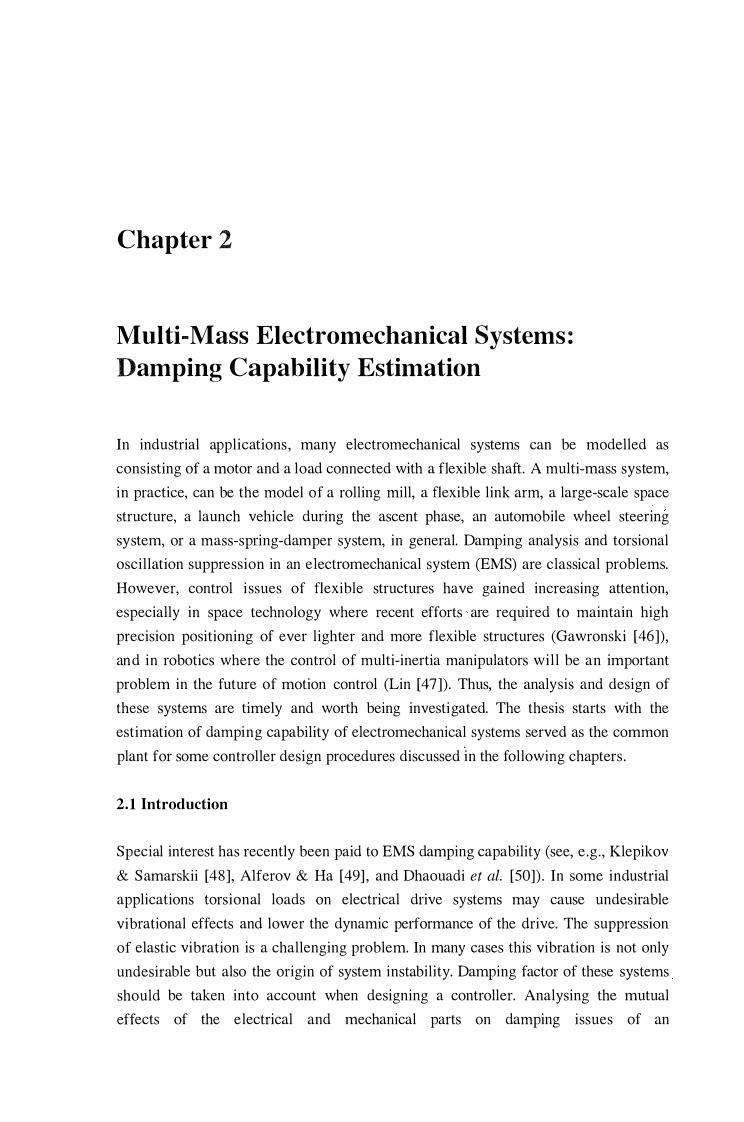
In the same way, by linearising the motor speed-torque characteristics around its
operation point P , as shown in Figure 2.1, and using the dynamic stiffness � of the
linearised speed-torque characteristics (2.3) , the general model for a motor electro
magnetic process can be given by Kljuchev [54] :

Chapter 2. Multi-Mass EMS's: Damping Capability Estimation 10
p f3 = -dT/dro
T
Figure 2. 1 . Dynamic stiffness of a linearised speed-torque characteristics .
(2.4)
where � is the motor electromagnetic time-constant.
2.2 .2 An n -mass electromechanical system model
In some fields of robotics such as space robot manipulators, robust control techniques
are required to obtain a stable and quick motion response. Since the robot total weight
is limited due to the allowable transport capability of space rockets, the stiffness of the
manipulator flexible structures is reduced and its motion tends to vibrate because of
the system small stiffness. To simplify the mathematical description, a model of
multiple mass spring system of Figure 2.2 is introduced for modelling the dynamic
behaviour of a flexible link arm. An industrial steel rolling mill can be represented by
the same structure. The state equations describing such a system can be written as (a
dot denotes the time derivative):
. 1 ( co� =- T- �2) , Jl
�2 = K12Cco1 -ro2) ,

Chapter 2. Multi-Mass EMS's: Damping Capability Estimation 11
(2. 5)
where 11 and co1 are the motor moment of inertia and speed,
Ji and co1, ( i = 2, . . . , n) are the i -th moment of inertia and speed,
Ku+ 1 ( i == 1, . . . , n- 1 ) are the stiffness of the coupling shaft between the i -th
and ( i + 1 )-th masses, and
T, Tv and I;,i+I are the motor torque, disturbance torque, and elastic torque (or
reaction torque in Nomura et al. [57]) of the i -th shaft, respectively. Note that all the viscosities B1 (i = 1 , . . . , n) of the i -th mass, and Bi,i+l (i = l, . . . , n - 1 ) of the i -th shaft
are omitted here, they will be considered in Section 2.6. The block diagram an n -mass
electromechanical system is shown in Figure 2.3 in the case neglecting the load
disturbance (TL == 0) . The compensation of the load torque influence, e.g. arm
disturbance rejection in a multi-mass resonant system (Matsuoka et al. [58]) , will be
discussed in the following chapters .
2.3 EMS characteristic equation in dimensionless space
In this section the characteristic equation of the structure of Figure 2.3 is derived in
dimensionless space.
T
Jl
rol ro2 ron-1 Kn-l,n
Figure 2.2. Multiple mass spring system.

Chapter 2. Multi-Mass EMS's: Damping Capability Estimation 12
2.3. 1 EMS characteristic equation
Consider first the two-mass system. An equivalent manipulation gives the simplified
block diagram, as shown in Figure 2.4, with
where ( Jl/2
Q = K Jt +12 N 1 2 J J 1 2
is the two-mass system natural resonant frequency, and
(2.6)
(2.6a)
(2.6b)
is the mass ratio in this case. The characteristic equation of the system of Figure 2.4 is
found as
�(s) = 1 + �s + BG1 (s) = 0. (2.7)
Figure 2.3 . An n -mass electromechanical system model.
CDI l+Tes G1(s)
Figure 2.4. Equivalent block diagram.

Chapter 2. Multi-Mass EMS 's: Damping Capability Estimation 1 3
In the case of a two-mass EMS, (2.7) can be put in the form:
where T = 1 "L = yJ1 is the system electromechanical time-constant. The same m p p '
procedure can be applied to a three-mass system with
where
is the three-mass natural resonant frequency,
Q _ K l1 + l2 Q _ K l2 + l3 ( Jl/2 ( Jl/2
12- 12 J J ' 23 - 23 J J I 2 2 3
are the first and second mode resonant frequencies,
is the mass ratio, and
y = J"L =
]1 + ]2 + ]3 JJ ]1
The three-mass system characteristic equation can then be obtained:
�3 (s) = �T111s6 + T111s5 + (y + a1Q��J;n)s4 + a1Q�T111s3 + + (yb1 + Te�nQ� )Q�s2 + Q�T111S + Q� = 0.
(2.9)
(2.9a)
(2.9b)
(2.9c)
(2.9d)
(2. 1 0)

Chapter 2. Multi-Mass EMS's: Damping Capability Estimation 14
The characteristic equation of an n -mass electromechanical system model can be
derived in the same way. For a chain of resonant blocks, the transfer function G1 (s)
can be written in the form
(2. 1 1 )
where ai > 0 , hi > 0 , i == 1, 2, ... , n - 2 ,
(2 . 1 2)
is the natural resonant frequency,
(2. 1 3)
i s the total moment of inertia, and
(2. 1 4)
is the mass ratio . The characteristic equation of the n -mass electromechanical system
model of Figure 2.3 can then be obtained:
Lln (s) = J1s(1 + �s)D(s) + �N(s) = _ TT 2n T ,2n-t ( n2 TT ) 2(n-tl r.2 T ,2n-3 ( ,/_ n4 TT ) 2(n-2l - e ms + m.s + y +��>tw e m S +at�>tw m's + 'Y0t +��>tw e m S + . . .
+("'b +a n,2(n-2)TT )s4 +a n,2(n-2)T 83 +("'b +Q2(n-!)TT )s2 +Q2(n-lly s+Q2(n-1) = O I' n-3 n-2 N e m n-2 N m i' n-2 N e m N m N ' (2. 1 5)
where the system electromechanical time-constant is defined as :
(2. 1 6)

Chapter 2. Multi-Mass EMS's: Damping Capability Estimation 15
2.3 .2 Dimensionless space
In the remainder of this chapter the following per-unit notation, proposed by Kljuchev
[54], is employed:
(2. 17)
The n -mass EMS characteristic equation then has the form:
A ( ) 2n 2n-J ( ) 2(n-l) 2n-3 ( b ) 2(n-2) Dn p = 't/"CmP + 'tmP + 'Y + al'te 'tm p + al'tmP + y 1 + a2'te 'tm p + . . .
+ (ybn-3 + an-2'te 'tm) P4
+ an-2'tmP3 + (ybn-2 + 'te 'tnJ P2
+ 'tmP + 1 = 0.
(2. 1 8)
For a two-mass EMS system (n = 2 , a1 = 1 , b1 = 0) the characteristic equation in
dimensionless space is obtained:
(2. 1 9)
and for a three-mass system (n = 3) :
Ll3 (p) = 'te 'tmP6 + 'tmP5 + (y + al'te 'tm)P
4 + al'tmP3
+ (ybl + 'te 'tm )P2
+ 'tmP + 1 = 0 '
(2.20)
where a1 and b1 are given in (2.9d) with 2<a1 , 0<h1 <2.
2.3 .3 EMS with a negligible electromagnetic inertia
The electromagnetic process in some DC and AC servo motors usually have a
negligible inertia and thus, results in very small values of 'te ('te = 0) . In this case, the
n -mass EMS characteristic equation (2. 1 8) is rewritten as
(2 .21 ) and particularly, for a two-mass system
(2.22)

Chapter 2. Multi-Mass EMS's: Damping Capability Estimation 16
and for a three-mass system
(2.23)
2.4 Maximal damping conditions
The discussion on the estimation of damping properties of an EMS starts with some
definitions.
2.4. 1 Definitions
In general, the characteristic equation (2. 17) of an n -mass EMS has n pairs of roots
Pi = -ai + jQi and Pi = -cri- jQi, i = l, . . . , n , where i = -1 , and cr; and Qi are non-
negative real numbers . Each pair of roots can be either complex-conjugate or real. For
estimating damping properties of an EMS the following concepts are introduced:
Definition 2 . 1 . Damping factor of a pair of complex-conjugate roots, Pi = -ai + .iO.; and P; = -cr;- JO.;, is the value
(2.24)
where <I>; is the angle illustrated in Figure 2.5.
Im(p)
83······ •..• ,_ ........
Re(p)
Figure 2.5 . Multi-mass system damping factor

Chapter 2. Multi-Mass EMS's: Damping Capability Estimation 17
Definition 2 .2 . (Alferov & Ha [49]) Damping factor of a multi-mass system is the
minimal value of damping factors 8i (Figure 2.5):
8 = min(8J. l�i�n
(2.25)
Definition 2 .3 . Dominant roots of a multi-mass system are the pair of complex
conjugate roots of the characteristic equation (2. 1 8) that correspond to the system
damping factor (2.25) .
Definition 2.4. Maximal damping of an electromechanical system is the case when the
electrical and mechanical parts have a common damping factor (Strelkov [59]) . A
maximal damping case of an n -mass electromechanical system of Figure 2.3 occurs
when all the complex -conjugate roots of the characteristic equation (2. 1 8) have the
same damping factor.
Definition 2.5. Complete damping of an electromechanical system is the case when all
the roots of the characteristic equation (2. 1 8) are located on the negative real axis . It can be a special case of maximal damping when the common damping factor is equal
to unity.
Definition 2 .6. Critical value Ycr of the mass ratio of an electromechanical system is a
the value of the mass ratio y at which complete damping corresponds to a multiple
root of the characteristic equation.
2.4.2 Maximal damping of an n -mass EMS
Theoretical calculations and experiments indicate that maximal damping of a two
mass EMS depends on the mass ratio y . The critical value of y is found equal to 5 for
the case considering the electromagnetic time constant 'te or equal to 9 for the case
neglecting --ce as given in Kljuchev [54] . The root loci for two-mass EMS's and
analytic expressions for system parameters at maximal damping are given in Alferov
& Ha [49] . The question arises as to whether these results can be extended to the
general case of n masses.

Chapter 2. Multi-Mass EMS's: Damping Capability Estimation 18
Theorem 2 .1 . (Maximal damping) A maximal damping case for an n -mass EMS of
Figure 2.3 with the characteristic equation (2. 1 8) and the mass ratio y defined in
(2. 14) is possible at the following system parameters:
(2.26)
and the maximal damping factor in this case is
(2.27)
Proof" In the general case, a maximal damping case can be found at a mu1tiple root
- ( 8 ± .i�) /rr: of the EMS characteristic equation (2.18). Thus, the system
parameters at possible maximal damping can be obtained by identifying the
coefficients of (2. 1 8) and the expansion of ( rr:2 p2 + 28rr:p +It. The fol lowing
equations are obtained:
2n 1e1m='t ' 't = 2n8rr:2n-I
m '
Y + a 't 't = n't2(n-I) + 282n(n - 1)'t2(n-I) 1 e m '
a1'tm = 28n(n - l)rr:2n-3 + 4
83n(n -l)(n - 2)rr:2n-3
, 3
'tm = 2nfu,
where a feasible solution can be found at {'te 'tm = 't = 1 , 'tm = 2n8,
y = 1 + 4(n2 - 1)82 I 3.
(2.28)
Thus, for a given mass ratio y > 1 , the EMS time-constants at maximal damping are
found dependent on y as in (2.26) with the damping factor given in (2.27) .

Chapter 2. Multi-Mass E.'MS's: Damping Capability Estimation 19
Theorem 2.2. (Complete damping) A complete damping case for an n -mass EMS of Figure 2.3 with the characteristic equation (2.18) is possible at a critical value of the mass ratio
4n2 -1 'Y = "fer = 3
when the system time-constants are given by
1 "Cm = "Cm,cr = .Jl + 3y = 2n, "Ce = "Ce,cr = -- .
'tm,cr
(2.29)
(2.30)
Proof The complete damping case is possible when the system damping factor 8 = 1 . Assigning unity for the left hand side of (2.27) gives the critical value of the mass ration as in (2.29) . Substituting this value into (2.26) gives the critical values of the time-constants (2.30) .
Theorem 2.3. (Case "C e = 0) A maximal damping case for an n -mass EMS of Figure 2.3 with the characteristic equation (2.2 1 ) , when the electromagnetic time-constant 'te is negligible, is possible at the following electromechanical time-constant
2n-J * -
't = 't = y4n-4 m. m '
and the maximal damping factor is found to be
8 = 8* = .fi - 1 .
2(n- 1)
The critical value of the mass ratio at complete damping for this case is
"fer = [1 + 2(n-1)]2 .
(2.3 1 )
(2.32)
(2.33)
Proof In the case 'te = 0, a possible maximal damping case takes place when the characteristic equation (2.20) has a (n - 1) -multiple root at - ( 8 ± j.J1- 82 ) /1: and a real root at -1/1:. Thus, the system parameters can be obtained by identifying the

Chapter 2. Multi-Mass EMS's: Damping Capability Estimation 20
coefficients of (2.2 1 ) and the expanswn of ('Tp + 1)(1:2p2 + 20'tp + l)n-l . The following equations are obtained
'Y = 't2(n-l ) + 28(n _ l )'t2(n- 1 ) ,
I where a feasible solution is found at 'T = y 4Cn-l) and thus, the value of the electromechanical time-constant is obtained as in (2.3 1 ) with the maximal damping factor ()* given by (2.32). The value of ()* achieves unity at complete damping when the mass ratio y is equal to its critical value given in (2.33) .
Remark 2 .1
From (2.29) and (2.33) , there is a possibility of complete damping in a two-mass EMS (n = 2 ) when the mass ratio is equal to 5 taking into account electromagnetic inertia, and to 9 neglecting 'te . The result is well-documented in Soviet literature (Kljuchev [5 1 ]) .
Remark 2.2
For a three-mass EMS (n = 3 ) , the critical value of the mass ratio "fer is found by the same formulae to be 3 5/3 considering 'te , and 25 when 'te = 0 (Ha [55]) .
2.5 Root loci of multi-mass electromechanical systems
In this section, the influence of the system parameter variations on damping capability is investigated using the classical root locus method. In order to plot the root distribution of a characteristic equation �(s) = 0, depending on a varying parameter K , following the Evans root locus principles (Kuo [60]) , it is required to put the equation �(s) = 0 into the form
�(s) = 1 + KG(s) = 0 , (2.34)
where G(s) is a rational function of s . For an n -mass EMS of Figure 2.3 , the characteristic equation (2. 1 8) in dimensionless space can be brought into the form

Chapter 2. Multi-Mass EMS's: Damping Capability Estimation 21
(2.34), where the varying parameter is the electromechanical time-constant 'tm . In fact, (2. 1 8) can be rewritten
� (p) = y(p2(n- 1 ) + b p2(n-2) + +b p4 + b p2 ) + 1 + 't ('t p2n + p2n-l + a 't p2(n-1 ) + n 1 " · n-3 n-2 m e l e
The root locus equation is then obtained as
2.5. 1 Root loci of two-mass electromechanical systems
For a two-mass system, the root locus equation (2.35) becomes
A ( ) - 1 p('tep + l )(p2 + 1 ) _ 0 02 P - + 'tm 2 - ·
'YP + 1 (2.36)
Using (2.27) and (2.26), the maximal damping factor o* and corresponding timeconstants <� and < are found dependent on the mass ratio "{ :
� * - Ji=l * - �1 * - 1 U - , "'Cm - 2-v"{ - l , "'Ce - r;:-:1 '
2 2-vy - 1 (2.37)
with the critical value "{ cr=5 given by (2.29). Figure 2.6 shows the root locus of twomass systems with the mass ratio "{=3<"fcr ' and "'Ce = 0. 2 < < (Figure 2.6(a)), "'Ce = < = 0. 7 (Figure 2.6(b)), and "'Ce = 1 > < (Figure 2.6(c)). Maximal damping corresponds to a multiple root of the characteristic equation. Hence, it takes place at minimax or saddle points of the root locus (Kuo [60]) as observed in Figure 2.6(b) . The location of these points is given in Alferov & Ha [49] :
(2.38)

Chapter 2. Multi-Mass EMS's: Damping Capability Estimation
2
1 .5
0.5
0 Re(p) -0.5
-1
-1 .5
-2 -2.5 -2 -1 .5
( 0.5 .
-0. 5
-1
- 1 . 5 L-----'----'-----'---�---' -5 -4
-1 -0.5 0
-3
0:. ]'
0
-2 -1 0
(a)
3
2
0 Re(p) -1 . -2
-3 - 1 -0 .8 -0 .6
0
(b) (c) -0.4 -0 .2
Figure 2.6 . Two-mass EMS root locus with y=3<Ycr : (a) 'te = 0. 2 < < , (b) 1: e = < = 0 . 7 , and (c) 1: e = 1 > < .
22
8 .§
0
0
where the mass ratio "{ <"fcr=5 . Complete damping of two-mass systems when "{ <"fer is not obtained except in the critical case (Y=Ycr=5, 'te = 'te cr = 0. 25) . This special case is depicted in Figure 2.7 where a multiple root is found at p = -1 . The two-mass EMS root loci with y =l 0>Ycr and 'te = 0. 1 < < , 'te = < = 0. 1 67 , and 'te = 1 > < are shown in Figure 2.8(a), Figure 2.8(b) , and Figure 2.8(c), respectively. If the mass ratio is greater than y cr=5, complete damping is possible at small values of the electromagnetic time-constant (Figure 2.8(a)) . As shown in Figure 2.8(b) , maximal damping in the case y >y cr coincides with complete damping which occurs at the two saddle points (Alferov & Ha [49]):
(2.39)

Chapter 2. Multi-Mass EMS's: Damping Capability Estimation
4
3
2
0
-1 -2
-3
-4 -3
2 \ . .. --01------Re(p)
-1
-2
p=- l'� .
-3 '---·--'------'------'-----'-----'----3 -2 .5 -2 - 1 . 5 -1 -0. 5 0
0
Figure 2.7. Two-mass EMS root locus with "{="fcr=5 and "Ce = 'te,cr = 0 .25 .
3 r---�---�--�--�--, �
2
0 Re(p)
-1
-2
-3 - 1 0 - 8
\�\ _, _____ ...... . . . .. . . .... � Re(p)
. .. ......___ .,,._,�,, psi
-2.5 -2 -1 .5 -1 -0.5
(b)
0
E7 ..§
0
-6 -4 -2 0
(a)
(:;:; 2 '--' s 1 . 5 .....
0.5
0 0
0.5 Re(p)
-1
1 . 5
-2 -0.8 -0.6 -0.4
(c) -0.2
Figure 2 .8 . Two-mass EMS root locus with "{=lO>y cr : (a) 'te = 0. 1 < 1: : , (b) 'te = < = 0. 1 67 , and (c) 'te = 1 > < .
0
23
8 s ......
0

Chapter 2. Multi-Mass EMS's: Damping Capability Estimation 24
The root locus equation for two-mass systems when 'te = 0 is written as
(2.40)
Equations (2. 3 1 ) , (2 .32) give the maximal damping parameters
(2.4 1 )
with the critical value y cr=9 obtained from (2.33). The root locus with the mass ratio "{ =4<"fcr ' "{="fcr=9, and y= l 3>"fcr is shown in Figure 2.9(a), Figure 2 .9(b), and Figure 2.9(c), respectively. Complete damping of a two-mass EMS with negligible 'te
takes place at large values of the mass ratio "{ ?:: "{ cr = 9 . The values of the electromechanical time-constant 'tm at complete damping can be determined from
(2.40) and the saddle points (Alferov & Ha [ 49]) :
[ ]1 /2 [ ]1 / 2 - -
y - 3 + �(y - l )(y - 9) - - y - 3 - �(y - 1)(y - 9) Pv� - , P�2 - . (2.42) . 2y . 2y
At small values of the mass ratio "{ (y<5 for 'te >O, or y<9 for 'te = 0) , two-mass EMS damping is incomplete and maximal damping corresponds to the value 8max at
the tangent from the coordinate origin with the root locus branch containing the dominant roots (Figures 2.6(a) and 2.9(a)) (Alferov & Ha [49]).
2.5.2 Root loci of three-mass electromechanical systems
For three-mass systems, (2.35) is written as following
(2.43)
where a1 and b1 are giVen in (2.9b). The maximal damping factor 8* and * * corresponding time-constants 't m and 't e are determined using theorem 2. 1 and
equations (2.27) and (2.26):

Chapter 2. Multi-Mass EMS's: Damping Capability Estimation
0.5
0
-0.5
8max 0.5
o . . . . . . . . . . . . . . . . . . . . . . . . . . . . . . . . . ��:t:= o Re(p)
-0.5
-1 -4
( 'tm=l.73 � · . . . . . . . . . . . . . . . . . . . . 'ri�-6.58 . '
.
Re(p) ... ,......__
-3
0
( -2 -1 0
(a)
0.5 ( �( �ml f o . . . . . . . . . . . . . . . . . . . . ....... .......................... . . . . . . . . . . . . . . . �-
Re(p) ps2 . psi \. 0
-0 .5
-1 �----�----�-----�----� -2 -1 .5 -1 -0.5 0
-1 L---'----'----'-----'------'----------' -3 -2.5 -2 -1 .5 -1 -0.5 0
(b) (c)
Figure 2 .9 . Two-mass EMS root locus with 'te = 0 : (a) y=4<y cr ' (b) "f='Ycr=9, and (c) y= 1 3>Ycr ·
25
s: * 1 Fe * 3 F * 1 u = - - y - 1 ) , 'tm = - - (y - 1 ) , 'te = -,-, ,
4 2 2 2 'tm (2.44)
and the critical value "( cr=3513 obtained from (2.29) (Ha [55]) . The root locus for the case "( =7<'Ycr is shown in Figure 2 . 1 0 where incomplete damping is observed. In the critical case, and "( ="( cr=35/3 and 'te = 'te,cr = 0. 1 67, a multiple root p = - 1 is found at 'tm = 'tm,cr = 6 as depicted in Figure 2. 1 1 . The root loci for the case "(= 1 5>Ycrwith 'te = 0. 1 3 > < , 'te = < = 0 . 146 , and 'te = 0. 2 > < are represented in Figure 2 . 1 2(a) ,
2 . 1 2(b) , and 2 . 1 2(c) .

Chapter 2. Multi-Mass EMS's: Damping Capability Estimation
4
3 2
1 · \ 0 1------
Re(p) -1 c -2
-3
-4 �----�----�---�--� -4 -3 -2 - 1 0
0
Figure 2 . 1 0. Three-mass EMS root locus with "{=7<Ycr ·
2
\, �· ··-.._ 0
( \:. 0
Re(p)
-1
-2
-3L---�----�--�-----�--� -5 -4 -3 -2 0 - 1
Figure 2 . 1 1 . Three-mass EMS root locus with y =35/3=y cr .
26
While damping capability in three-mass systems increases at small values of the electromagnetic time-constant 1: e , complete damping is impossible except in the critical case. When 1: e = 0 , the three-mass EMS root locus equation (2.41) is written
as :
(2.45)
Theorem 2 .3 and equations (2.3 1 ) , (2.32) give the maximal damping parameters :
* - 5/8 <;;: * - -JY - 1 'tm - 'Y ' u - . 4
(2 .46)

Chapter 2. Multi-Mass EMS's: Damping Capability Estimation
4
3
2
0
-1
-2
-3
-4 -6
4
3
2
0 Re(p) - 1
-2
-3
-4 -8
_____ .... . . . Re(p)
-5 -4 -3
(b) -2
-6
c
- 1 0
-4
(a)
0: 4
s 3 -
2
0 0
-1
-2
-3
-4 -4
-2
Re(p)
-3
0
0
-2
(c) - 1
Figure 2. 1 2. Three-mass EMS root locus with y= 1 5 : (a) 'te = 0. 1 3 > < , (b) 1: e = < = 0. 146 , and (C) 1: e = 0. 2 > < .
27
0
0
The critical value of the mass ratio is found from (2.3 1 ) to be y cr=25 with complete damping possible at 'tm = 'tm cr = 7.48 . Figure 2. 13 (a) and 2. 1 3 (b) show the root locus with y=9<Ycr and y =25=Ycr · The root locus for the case y =36>Ycr is depicted in Figure 2. 1 4( a) and 2 . 14(b) with different values of a1 and b1 • It is observed that with y >y cr complete damping is possible at some values of a1 and b1 (Figure 2. 14(b) ).
2.5.3 EMS multi-parameter root loci
When operating, electromechanical systems are subject to parameter variations. The influence of parameter perturbations on the characteristic equation roots can be examined by using a family of root loci with several varying parameters.

Chapter 2. Multi-Mass EMS's: Damping Capability Estimation
1 . 5
0 .5
0
-0.5
-1
- 1 .5 -5
2
1 .5
0 .5
0
-0.5
-1
-1 . 5
-2 -8
0: \ � s ...... ( /' 0.5 ,l_ 'tm=7.48 ·. :
0 � ·-Re(p) 0 Re(p) p=-0.67
.. ,
(( \ -0.5
� � I -4 -3 -2 - 1 0
-1 -5 -4 -3 -2 -1
(a) (b)
Figure 2 . 1 3 . Three-mass EMS root locus when 'l:e = 0 : (a) y=9<y cr > and (b) "( =25="( cr .
2 �
c� a1=4.47 8 a!=5 .41
( s 1 .5 b1=0.89 >--< bJ=0.91
(_ 0.5
0
Re(p) o mm m ' 0 0 '" ' ;"''\. Re(p)
\_ -0.5
-1
- 1 .5
-6 -4 -2 0 -2 -8 -6 -4 -2
(a) (b)
Figure 2 . 1 4. Three-mass EMS root locus with 'l:e = 0 and y=36: (a) a1=4.47, b1 =0.89; (b) a1=5 .4 1 , b1 =0.9 1 .
\ 0
28
� 8 s ......
0
� 8 s
>-<
0
Based on the sharpest possible bounds provided by the well-known Kharitonov polynomials [5] , the robust root locus method, proposed by Barmish & Tempo [6 1 ] , exploits a two-dimensional gridding of a bounded set o f the complex plane for generating the multi-parameter root loci . A computational technique for the robust root locus is described in Tong & Sinha [62] . Applying the robust root locus method requires that each coefficient of the nominator and denominator of the function G(s)

Chapter 2. Multi-Mass EMS's: Damping Capability Estimation 29
in (2.34) depends on one and only one perturbation parameter in order to result in an interval characteristic polynomial (Barmish & Tempo [61 ]) . To maintain the physical meaning in parameter variations and to avoid the conservative requirement on the relations of the monic characteristic equation coefficients with the perturbation vector, the classical multi-parameter root locus method is used in this section. The influence of variations of the load moment of inertia Jn and dynamic stiffness � of
the motor speed-torque characteristics is considered in terms of root loci with varying values of the mass ratio y and electromechanical time-constant "Cm . The multi-parameter root loci for the two-mass case with "Ce = 0 are shown in Figure 2. 1 5,
where complete damping can be observed on the negative real axis with some values of "Cm .
0.5
0
0.5
4<'tm<8
7<y<l l
Re(p)
-1 �--�--�--�---4---�--� -3 -2.5 -2 -1 .5 -1 -0.5 0
0
Figure 2. 1 5 . Two-mass EMS multi-parameter root loci with "Ce = 0 , "Cm = var . , y = var .
Taking into account the electromagnetic inertia, the loci when "Ce = 0. 25 , 't m = var . , y = var. are shown in Figure 2. 1 6(a) and when y = 5 , "Ce = var . , 'tm = var. in Figure 2. 1 6(b) . Damping c apability increases at smaller values of 'te . The three-mass system root loci with varying y and 'tm are shown in Figure 2. 17(a) when'te = 0. 1 67 and 2 . 17 (b) when 1: e = 0 . While complete damping is possible only in the critical case considering the electromagnetic inertia, it can be achieved at y >y cr and some values of 'tm with 'te = 0 . The sparse region around the real axis (Figures 2. 1 5-2. 1 6) or at the
centre of the root loci (Figure 2. 17) indicates that the roots of the characteristic equation and hence, the system dynamic properties, at maximal damping are sensitive to parameter variations, eg. changes in the mass ratio, the electromechanical and

Chapter 2. Multi-Mass EMS's: Damping Capability Estimation 30
electromagnetic time-constants. This is explained by the fact that these roots are
multiple [56] . The dense region near the imaginary axis implies that the dominant
roots of a multi-mass EMS are less sensitive to varying environments and can be used
for the purpose of model reduction when designing a robust controller for these
systems. It should be noted that this root region contrast is not specified with the
robust root locus method.
2<'tm<6 3 2<y<6 2 -
-1
-2
-3
0
0. 1 <'te<0.4 2 2<'tm<8
0 Re(p)
-1
-2
-4 L-----�----�----��--� -3 -4
4
3 4<'tm<8 9<y< l 3
2
0 Re(p)
-1 -2
-3 -4 -5 -4
-3 -2
(a)
- 1 0 -1 0 -8 -6 -4 -2
(b)
Figure 2 . 1 6. Two-mass EMS multi-parameter root loci with (a) 'te = 0. 25 , 'tm = var. , y = var . ; (b) "{ = 5 , 'te = var. , 'tm = var.
2 "'"' 8 s 1 .5 .....
0.5
0 0
-0.5
-1
-1 .5
-2 -3 -2 - 1 0 -5
(a)
5<'tm<l0 23<y<27
Re(p)
-4 -3 -2 (b)
( / ;,,· . ·:'(� '• . <, ' • '..J
("'( - 1
Figure 2 . 17 . Three-mass EMS root loci with 'tm = var . , "{ = var . :
(a) "Ce = 0. 1 67 , (b) "Ce =: 0 .
0
0
0; :g
0
0

Chapter 2. Multi-Mass EMS's: Damping Capability Estimation 31
2.6 Viscous friction influence
Although friction maybe a desirable property, as it is for brakes, it is generally an
impediment for servo control. The field of control has long incorporated sophisticated
investigations of other contributions, eg. multi-mass dynamics, to the forces of motion
(Armstrong-Helouvry et a l. [63]) . The influence of viscous friction on two-mass EMS damping capability is considered using the mass-spring-damper model shown in
Figure 2 . 1 8( a) with the block diagram of Figure 2. 1 8(b ). The state equations with
TL == 0 can be written as :
13 --
l+Tes
Jl B l
rol K1 2 B l 2
(a)
(b)
ro2
K12 - + B 12 s
Figure 2. 1 8 . Two-mass system with viscosities:
(a) spring-mass-damper model, (b) block diagram.
(2.47)

Chapter 2. Multi-Mass EMS's: Damping Capability Estimation 32
where B1 , B2 , and B12 are viscous friction coefficients of motor, load, and the
coupling shaft, respectively. The system characteristic equation can be found as :
(2.48)
where the natural frequency Q N and the mass ratio y are given in (2.6a) and (2.6b ) .
By introducing further per-unit coefficients
(2.49)
the two-mass EMS characteristic equation (2.48) can be written in dimensionless
space as follows:
fl2 (p) = 't/CmP4+ [J..l'te 'tm + ( �1 + Jh_)yte + 'tm ]P3 + y - 1
+ [(1 + � I + Jh_)y + J..l'te (� I + �2 ) + ('te + J..l)'tm + � 1�2 L�]p2 + y - 1 y - 1 'tm
y2 1 + [J..l + V + 'tm + ('te + J..l) (�1 + �2 ) + �1 �2 --]p + �1 + �2 + 1 = 0. Y - 1 'tm
(2.50)
The root locus equation of the form (2.36) can be derived for the case considering
viscous friction on the first shaft (motor) (B1 -:t- 0 , B2=B12 =0):
(2.5 1 )
and the case considering the viscous friction pair on the second shaft (load) and the
coupling shaft (B1=0, B2 -:t- 0 , B12 :f. 0 ) :

Chapter 2. Multi-Mass EMS's: Damping Capability Estimation 33
(2.52)
The multi-parameter root loci for a two-mass EMS at y = y cr=5 with varying viscous
friction coefficient B1 are shown in Figure 2. 19 . As can be seen, viscous friction on
the motor shaft makes the dominant roots move closer to the imaginary axis and the
other two roots further in the left hand side of the complex plane. Thus, two-mass
EMS dynamics is sensitive to friction B1 .
2
0 Re(p)
-1
-2
-3 -3 -2.5 -2 -1 . 5 -1
2<tm<6 E; 0<�1<0.6 ,§
0
-0.5 0
Figure 2. 1 9 . Two-mass EMS root loci with viscous friction on the motor shaft
(y=5, 'te =0.25).
The root loci with varying viscous friction coefficient B2 on the load shaft are
depicted in Figure 2 .20(a). It is inherent that two-mass EMS dominant roots are less
sensitive to viscous friction B2 on the load shaft than to viscous friction B1 on the
motor shaft. The influence of varying friction coefficient B12 on the coupling shaft is
represented in Figure 2.20(b) when B2 = 0 , and in Figure 2.20(c) when B2 i= 0. The
root loci indicates that friction on the coupling shaft has similar effects as friction on
the motor shaft, i.e. sensitivity to any variations. EMS dynamics is observed not as
sensitive to viscous friction on the load shaft as to friction on the motor or coupling
shaft. However, damping capability of the system is more affected with friction on the
load shaft. As shown in Figure 2.20(a) and 2.20(c), complete damping does not exist
with the presence of viscous friction B2 .

Chapter 2. Multi-Mass EMS's: Damping Capability Estimation
' :/ I
2
0 Re(p)
-1
-2
-3 -3 -2.5 -2
3 .---�--�--�--�----�--. 2<'tm<6 :.:§;
2 0<J.1<0.6, �2"'0 ,§
0 1------Re(p)
-1
-2
-1 .5
(a)
2
-1
-2
2<'tm<6 :.:§; 0<�2<0.4 ,§
I t"- 0
-1 -0.5 0
-3 L---�--�--�--�----�� -3 L---�--�--�--�--�--� -3 -2.5 -2 -1 . 5 - 1 -0.5 0 -3 -2.5 -2 -1 .5 -1 -0.5
(b) (c)
Figure 2.20. Root loci with viscous friction on the load and coupling shaft ("{=5 , 'te =0.25) :
0
0
(a) B1=0, B2 ;t: 0 , B1 2 = 0 ; (b) B(=O, B2 = 0 , B12 ;t: 0 ; (c) B1=0, B2 ;t: 0 , B12 ;t: 0 .
34
In some industrial applications such as steel rolling mills or metal-cutting machines,
viscous friction on the load and coupling shaft may cause undesirable self-excited
oscillations. The root loci at larger values of the mass ratio "{ show that this influence
is reduced as the mass ratio increases.
Chapter 2. Multi-Mass EMS's: Damping Capability Estimation 35
2. 7 Illustrative examples
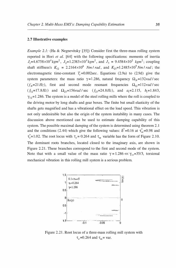
Example 2. 1 : (Ha & Negnevitsky [35]) Consider first the three-mass rolling system
reported in Hori et al. [64] with the following specifications: moments of inertia
J1 =4.6758x10⁴ kgm2 , J2= 1 .2383x 104 kgm2 , and 13 = 9.4584x 10² kgm2 ; coupling
shaft stiffness's K12 = 2 .2 1 64x108 Nm I rad , and K23=1 .2485x107 Nm I rad ; the
electromagnetic time-constant � =0.002sec . Equations (2.9a) to (2.9d) give the
system parameters: the mass ratio y= l .286, natural frequency 0.N=l 32rad I sec
(/�=2 1 Hz) , first and second mode resonant frequencies 0.12=1 12rad I sec
(fi2= 17 . 8Hz ) and 0.23= 1 56rad I sec (f23=24 .8Hz) , and a1=2. 1 1 5 , b1 = 1.843 ,
y1 2= 1 .286. The system is a model of the steel rolling mills where the roll i s coupled to
the driving motor by long shafts and gear boxes. The finite but small elasticity of the
shafts gets magnified and has a vibrational effect on the load speed. This vibration is
not only undesirable but also the origin of the system instability in many cases. The
discussion above mentioned can be used to estimate damping capability of this
system. The possible maximal damping of the system is determined using theorem 2 . 1 and the conditions (2.44) which give the following values : o* =0. 1 6 at <n=0.98 and
<= 1 .02. The root locus with 'te = 0.264 and 'tm variable has the form of Figure 2. 1 0.
The dominant roots branches, located closed to the imaginary axis , are shown in
Figure 2.2 1 . These branches correspond to the first and second mode of the system.
Note that with a small value of the mass ratio y = 1 . 286 << 'Ycr=3513, torsional
mechanical vibration in this rolling mill system is a serious problem.
0.5
0. 1 <1:m<5
'te=0.264 y=1.286
0 1----------------
-0 Re(p)
0.5
-1
1 .5 '------'-------'-------' -0.1 -0.05 0
Figure 2.2 1 . Root locus of a three-mass rolling mill system with 'te =0.264 and 'tm= var.
Chapter 2. Multi-Mass EMS's: Damping Capability Estimation 36
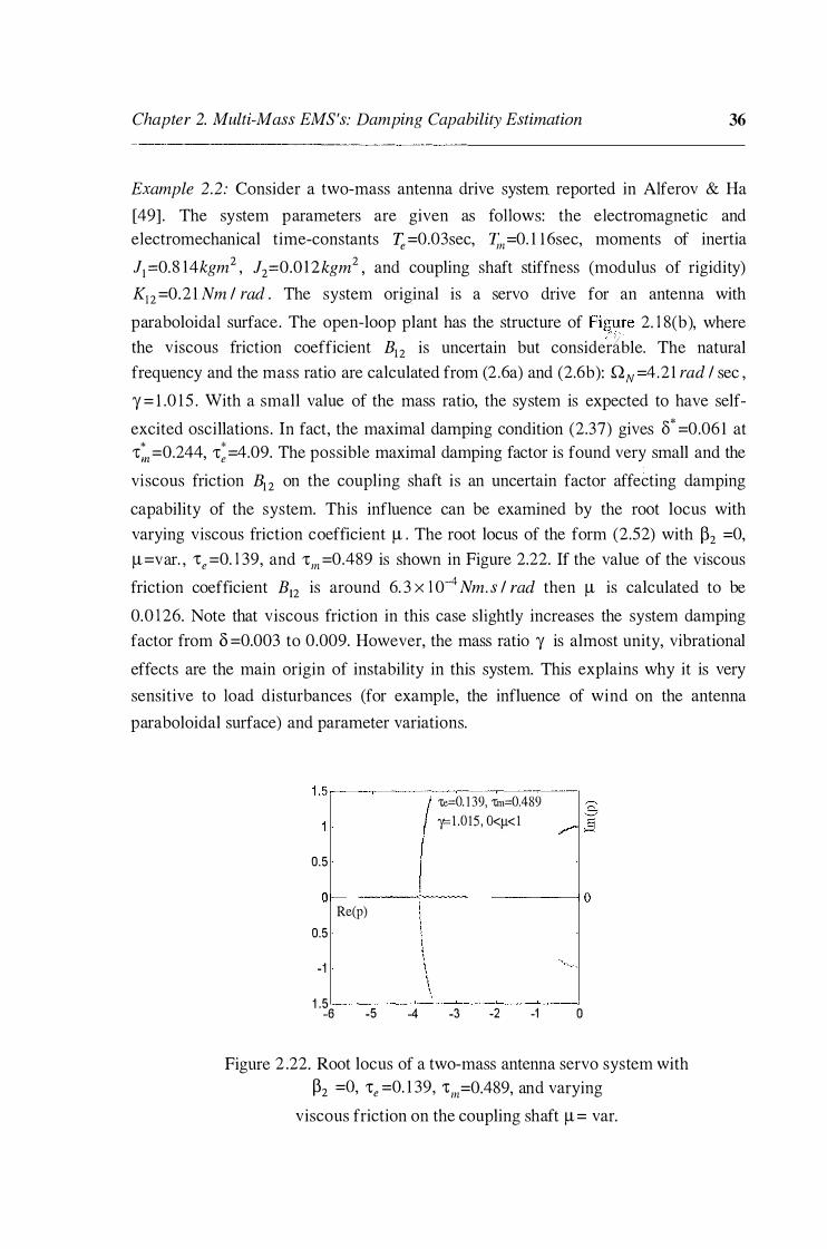
Example 2.2: Consider a two-mass antenna drive system reported in Alferov & Ha [ 49] . The system parameters are given as follows: the electromagnetic and electromechanical time-constants 7;,=0.03sec, Tm=0. 1 1 6sec, moments of inertia 11 =0.8 14kgm2 , 12=0.012kgm2 , and coupling shaft stiffness (modulus of rigidity) K12 =0.21 Nm I rad . The system original is a servo drive for an antenna with paraboloidal surface. The open-loop plant has the structure of Figure 2. 1 8(b ), where
7"
the viscous friction coefficient B12 is uncertain but consider�ble. The natural frequency and the mass ratio are calculated from (2.6a) and (2.6b): QN=4.21 rad I sec , "{= 1 .0 1 5 . With a small value of the mass ratio, the system is expected to have selfexcited oscillations. In fact, the maximal damping condition (2.37) gives 8* =0.061 at '!:=0.244, <=4.09. The possible maximal damping factor is found very small and the viscous friction B1 2 on the coupling shaft is an uncertain factor affecting damping capability of the system. This influence can be examined by the root locus with varying viscous friction coefficient � . The root locus of the form (2.52) with �2 =0, �=var. , 'Ce =0. 1 39, and 'tm=0.489 is shown in Figure 2.22. If the value of the viscous friction coefficient B12 is around 6. 3 x 1 o-4 Nm. s I rad then � is calculated to be 0.0 1 26. Note that viscous friction in this case slightly increases the system damping factor from o =0.003 to 0.009. However, the mass ratio "{ is almost unity, vibrational effects are the main origin of instability in this system. This explains why it is very sensitive to load disturbances (for example, the influence of wind on the antenna paraboloidal surface) and parameter variations.
0.5
'te=0. 1 39, "Cm=0.489
y.=l .015 , O<Jl<l
0 1--- ---:- -,� -----1 0 Re(p)
0.5
-1
1 .5 '----'----'-----'-----'-----'-----' -6 -5 -4 -3 -2 -1 0
Figure 2 .22. Root locus of a two-mass antenna servo system with �2 =0, 'Ce =0. 1 39, 1:m=0.489, and varying
viscous friction on the coupling shaft � = var.
Chapter 2. Multi-Mass EMS's: Damping Capability Estimation 37
2.8 Summary
In this chapter, the problem of estimating maximal damping capability in multi-mass electromechanical systems was systematically addressed. The concept of dynamic stiffness of a linearised speed-torque characteristics, proposed by Kljuchev, is used for modelling the electromagnetic process of a motor. Thus, an n -mass flexible structure dynamics can be represented by a general block diagram. By introducing the per-unit notation, the characteristic equation of n -mass systems can then be written in dimensionless space, depending only on the mass ratio and the electromagnetic and electromechanical time-constants in relative units.
The main contribution here is that the conditions for maximal damping and complete damping are determined in the general case. The values of the electromagnetic and electromechanical time-constants at maximal damping are found depending on the mass ratio y . Hence, the critical value of the mass ratio Ycr and the corresponding
system time-constants at complete damping can be derived. For two-mass systems, y cr is obtained equal to 5 in the case considering electromagnetic inertia 1: e , or equal to 9 in the case neglecting 'te , a result widely-known in Soviet literature. For three-
mass systems, the critical value of the mass ratio is 35/3 taking electromagnetic inertia into account, or 25 in the case 'te ::: 0 . There exists a theoretical possibility for
maximal damping, or complete damping if the flexible structure is not so complicated (eg. n == 2) and the electromagnetic time-constant is small enough. However, at maximal damping large values of the mass ratio y are required.
One important feature is the use of the classical root locus method to illustrate the cases of maximal and complete damping in two-mass and three-mass electromechanical systems considering or neglecting motor's electromagnetic inertia. The influence of variations in the electromechanical time-constant 'tm (eg. changes in
load inertia or dynamic stiffness of motor's speed-torque characteristics) on the root distribution of the system characteristic equation is directly observed on root locus plots . The multi-parameter root loci take into consideration other changing factors such as the electromagnetic time-constant and the mass ratio. It is obvious that at maximal or complete damping, which corresponds to a multiple root of the characteristic equation, the system dynamic behaviour is extremely sensitive to varying parameters . With a given mass ratio y, dominant root branches of the system
Chapter 2. Multi-Mass EMS's: Damping Capability Estimation 38
root loci are observed not affected by parameter variations as much as the branches containing other roots.
The inf1uence of viscous friction exerted on the motor, load, and coupling shafts is considered in dimensionless space using multi-parameter root loci. It is shown that two-mass system dynamics is more sensitive to friction on the motor and coupling shaft than friction on the load shaft. However, maximal damping of the system is seriously affected by friction on the load shaft. The oscillatory influence of viscous friction on the load and coupling shaft in two-mass systems is reduced at large values of the mass ratio.
A three-mass rolling mill system and a two-mass antenna servo drive system are used for the illustration purpose. In practice, the mass ratio value of electromechanical systems is usually much smaller than the critical value, as illustrated in the examples . The problem of increasing the damping capability in these systems becomes considerably important, especially for vibration suppression and the achievement of robustness to load and parameter variations. Furthermore, it should be noted that the generalised model (2.4) is applied to electric motors only under linearised conditions of the speed-torque characteristics.

Chapter 3
Robust Modal Control: an Overview
In multi-mass electromechanical systems, the suppressio!} of elastic oscillations and rejection of external disturbances are challenging problems. The influence of parameter and load variations , and nonlinearities may also deteriorate the system performance to an intolerable extent. Thus, these systems require a controller that can achieve specified signal levels in the face of uncertainty, or a robust controller. This chapter is devoted to the development of such a control method for electrical drive systems, especially for flexible structures.
3.1 Introduction
Dote in [65] noted that there has been a great effort in applying modern control techniques in motor control. Feedback control covers a large area in these applications. In high performance electrical drives, for example in the area of robotics, tool machines, and electrical servos, it is required to develop a controller that can provide high accuracy, fast response, and insensitivity to system parameter variations, changing load, torque disturbance and nonlinearities. Various control methods addressing these problems have been developed: loop gain shaping (Bailey & Hui [66]) , state feedback control (De Vegte [67]) , linear quadratic control (Anderson & Moore [68]) , model reference and adaptive control (Astrom [69]) , H= robust control (Kwakernaak [6]) , and variable structure systems with sliding mode (Utkin [7] , DeCarlo e t al. [70]) . (The issues relating to controllers using artificial intelligence tools , such as fuzzy logic or neural networks will be discussed in the following chapters). The conventional proportional-integral controllers cannot meet these requirements simultaneously. Adaptive controllers are effective to the control of the drive system whose model parameters are uncertain but sometimes it gives undesirable response [ 65] . The variable structure system method provides parameter insensitivity once the system is in the sliding mode but chattering is a problem.
Chapter 3. Robust Modal Control: an Overview 40
Furthermore, when the system uncertainty is larger than one taken into account in the design, the sliding mode does not exist (Furuta [7 1 ]) .
For applications in flexible structures, among the above methods, linear state feedback is of particular interest due to its design simplicity and its ability to assign a desired eigenstructure or modes to the closed loop system. That is why the method is also referred to as modal control (Kuzovkov [72]) . The objective of modal control is to determine the feedback gain matrix in the linearised state equation in such a way that all the poles of the closed loop system are desirably placed in the complex plane and thus , its transient response has a desired shape. In modal control, knowledge of the state variables is required. However, in practice, not all of these variables are readily measurable. On the other hand, the influence of external disturbances may deteriorate the steady-state performance of the control system and should be compensated for. Hence, it is required to incorporate observers with a modal controller to provide estimates of the unmeasurable state variables for pole-placement feedback control, and estimates of the disturbances for feedforward compensation control. Moreover, the eigenvalue assignment is dependent on entries of state matrices, and thus, modal control is sensitive to system parameters . Therefore, robustness of pole assignment techniques should be taken into consideration. This chapter addresses these problems using an approach called robust modal control. Its material is based on the works by Ha [9], Ha & Alferov [ 19 , 9 1 ] , Alferov & Ha [73, 75, 36] , and also in Alferov, Ha & Khusainov [74] . The design of a continuous and discrete-time robust modal controller with its applications in electromechanical systems are discussed in the following sections. Pros and cons of the proposed method and further suggestions will conclude this chapter.
3.2 Modal control
3.2. 1 Linearised model
Modal control requires a linear approximation of the controlled object dynamics . For a broad class of motion control systems the dynamic behaviour of the system variations about operation point values can be approximated by a time-invariant linear differential equation, or equivalently, a state model of the form:
x(t) = Ax(t) + Bu(t) + Dv(t)
y(t) = Cx(t) (3 . 1 )
Chapter 3. Robust Modal Control: an Overview 41
where x(t) E Rn is the state vector, u(t) E Rr is the control vector, v(t) E Rlf is the disturbance vector, and y(t) E Rm is the output vector; A E Rnxn is the system matrix,
B E Rnxr ' c E Rmxn ' and D E Rnxq .
In electrical drives, many systems can be described by, or reduced to the linearised model (3 . 1 ) . The linear state equations are given in Ha & Alferov [ 19] for a variety of electric motors used in servo systems. The typical motors widely used in position drives are DC motors. Consider a servo system including a converter, a DC motor, and its mechanism with the angular position as the output. The state and output equation can be written as:
- 1/� 0 0 0 Kef�. 0 0 ;
_ Bm/fm Kb/fm 0 0 -1/fm x(t) =
1/RaTa -KtfRaTa - 1/Ta 0 x(t) +
0 u(t) +
0 TL (t), (3.2)
0 1 0 0 0 0
y(t) = [O 0 0 l]x(t) ,
where the state vector is chosen as x(t) = [ e.I']J (0 ia e r (superscript T identifies a transpose), with the supply voltage e�'P , the motor speed co , the armature current ia ,
and the position angle e ; the control signal u(t) as the voltage applied to the voltage converter; and the external disturbance as the load torque TL (t) . The coefficient Kc is the converter voltage g ain, � is the converter time-constant, Bm i s the viscous friction coefficient, J m is the total moment of inertia, Kb is the motor back emf constant, K1 is the motor torque constant, Ra is the total armature resistance, Ta = La/ Ra is the electromagnetic time-constant, and La is the armature inductance. The model can be made simpler if Tc is negligible or a current converter is used (Alferov & Ha [75]).
In servo applications , DC motors are being gradually replaced by permanent magnet synchronous motors, sinusoidal or trapezoidal classes (brushless DC (motors) (Jahns [76]), since they have lower inertia, larger power rate, fewer spark problems and lower noise. While there are some differences in construction between the two classes of permanent magnet synchronous machines, a sinusoidal permanent magnet synchronous motor and a brushless DC motor are all synchronous machines with a Y
connected 3-phase stator and a permanent magnet rotor. In field-oriented or vector control (Boldea & Nasar [77]) , an independent (or decoupled) control of flux and torque of the motor is aG:complished through a coordinated change in the supply

Chapter 3. Robust Modal Control: an Overview 42
voltage and frequency. In permanent magnet synchronous machines, by field-oriented control, the stator current component ids in the d - q frame is made equal to zero. The
general voltage controlled model for permanent magnet synchronous drives can then be written as:
(3.3)
y(t) = [0 0 l ]x(t) ,
T where the state vector i s chosen as x(t) = [co iqs e J , the control voltage as the stator voltage component Vqs ( t ) , and the disturbance as the load torque TL ( t ) , and where Am is the magnet flux linkage amplitude, Lq is q -axis stator inductance, Rs is stator resistance, p is the number of pole pairs, and Kt = 3 p'Am/2 is the torque constant.
The model for a permanent magnet synchronous motor can be further simplified by using a current source inverter where iqs is a known quantity and serves as a control
signal to the motor in Ko et al. [78] .
For an induction motor with a current regulated Pulse Width Modulator the mathematical model in the rotating reference frame d - q can be linearised by using vector control (Tzou & Wu [79]) . In the constant torque region ids = canst , the state
model of a current-decoupled induction motor is written as [ 1 9] :
y(t) = [0 0 l]x(t) ,
where the state vector x(t) is chosen as in (3 .3) and the control signal i; (t) is the inverter input, and where Kt = 3 pL� /2 Lr is the torque constant, Ki is the inverter gain, � is the inverter time-constant, Lm is the mutual magnetising inductance, and Lr is the rotor inductance.
Consider the speed control of a two-mass servo drive of Figure 2. 1 8(b). Taking into account the influence of the load torque TL as the external disturbance, with the state

Chapter 3. Robust Modal Control: an Overview 43
T vector chosen as x(t) = [T ro1 �2 ro2 ] and the load speed ro2 as the output, the
state model for the system (2.47) can be written as (Ha [9]) :
-I -� 0 0 0 I'; r; l_ - BI Te 0 _l_ -I 0 11 � I; 0 x( t) =
Bl2 K1211 - B12B1 - Bl2 ( 11 + J2 ) BI 2BI - K\ 212 x(t) + (t) r�f" ( t) + Bl2 TL (t) , (3.5)
-T 11 11 .12 12 0 7; - 82 0 -I
0 0 I 7; 7; T
y(t) = [0 0 0 l]x(t) .
3.2.2 Modes, Controllability, and Observability
Recall that the state model for a system depends on the choice of a set of state variables, and thus is not unique. In fact, a new state vector z(t) can be defined by a nonsingular coordinate transformation x = Tz but the eigenvalues of the transformed system matrix T-1 AT and of A are the same because the characteristic equation does not change:
(3.6)
where In E Rnxn is the identity matrix. Of particular interest is the transformation U
required to diagonalise the system matrix A :
(3 .7)
where Ai, i = 1, . . . , n , are the roots of the open loop system characteristic equation:
It can be derived from (3 .6) that AU = UA , or
and by equating the i -th columns, we have
Chapter 3. Robust Modal Control: an Overview 44
(3 .9)
The solution ui of (3.9) is the i -th (right) eigenvector of the system matrix A with respect to the eigenvalue "Ai corresponding to a system mode. Thus, the transformation
U diagonalising A is called the (open loop) modal matrix. Assuming that the system (3 . 1 ) is free of disturbances (D = 0 ), with x = Uz , the transformed state equation is then written as :
z = Az + u-'Bu = Az + VTBu , y = CUz , (3 . 1 0)
where z = u-'x = VT x is the modal vector. The i -th columns vi of V = [v 1 , • • • , v n ]
are the left eigenvectors of A :
(3 . 1 1 )
and satisfy the following properties :
(3 . 1 2)
The linear system is controllable if and only if u-'B has no rows consisting entirely of zero elements, and it is observable if and only if CU has no columns consisting entirely of zero elements (De Vegte [67]) . The concepts of controllability and observability, first introduced by R. E. Kalman [80] , play an important role in modal control . Suppose that the i -th row of u-'B has only zero elements, then from (3.9) the i -th mode is uncontrollable, since it is not affected by the control. Similarly , suppose that the j -th column of CU has only zero elements, then the j -th mode i s unobservable, because it does not show up in the output. It i s known that the conditions of controllability and observability are expressed in terms of A and B, and A and C , respectively (De Vegte [67] , Kuzovkov [72]). The following theorem is very popular:
Theorem 3. 1 : The p air (A , B) is controllable if and only if the rank of the controllability matrix
(3 . 1 3)
is n . The pair ( C , A ) i s observable if and only if the rank of the observability matrix

Chapter 3. Robust Modal Control: an Overview 45
(3 . 1 4) is n .
3.2 .3 Pole assignment and feedback matrix
For the system (3. 1 ) with D = 0 , the state model and state feedback control are:
:X = Ax + Bu, y = Cx ,
u = -Kx ,
(3 . 15a) (3 . 1 5b)
where K E Kxn is the feedback gain matrix . The objective of state feedback control is to assign the closed-loop eigenvalues of the closed-loop matrix (A - BK) or the roots of the closed-loop characteristic equation
Ll(s) = !sin - (A - BK) I = 0 . (3 . 1 6)
The desired characteristic equation is found from the desired closed-loop eigenvalues Aci ( i = 1 , . . . , n ) :
(3 . 1 7)
The choice of the pole s "Ac,i is based the desired transient response of the closed-loop
response. There exists many criteria for such a choice. In the field of electrical drives, for example, the popular criteria are the binomial expansion, Butterworth polynomials, magnitude optimum principles, and Graham-Lathrop minimisation of the integral time absolute error (ITAE) (Terekhov [8 1 ]) . Transient performance and coefficients of normalised polynomials by those criteria are given in Appendix A. A comprehensive comparison between the magnitude and symmetric optimum criterion with others is discus sed in Umland & Safiudin [82] . After choosing the desired closed-loop poles, the elements of the feedback matrix K can be found by equating coefficients in (3 . 1 6) and (3. 17). In state feedback control, the condition for determining the feedback matrix K consisting of constant gains is the controllability of the pair (A , B) .

Chapter 3. Robust Modal Control: an Overview 46
For the single-input case (n = 1 ) , the design procedure comprises of two steps : (i) using a coordinate transformation to bring the state model (3 . 1 5a) to the companion
form with
0 0 0
A = (3 . 1 8) ' b = 0 0
1
and (ii) the feedback row vector kT = [ k1 k2 • . . kn J is then found as
(3 . 1 9)
where ai and ai are the coefficients of the open loop and desired closed-loop
characteristic polynomial, respectively. For multiple-input systems, a common technique is to reduce them in effect to single-input ones according to u = gw , where g is a vector of constant and w is a new single input. Then
x = Ax + Bu = Ax + (Bg)w = Ax + bw , (3 .20)
and g must be chosen such that (A , b ) is controllable.
An alternative technique for pole assignment is modal control which is based on modal transformation. Consider a single-input system with state feedback:
(3 .21 )
By using the modal transformation in (3. 1 0)-(3. 12) and feedback from the i -th and j -th modal variables zi , z 1 with gains ki , k
.i to generate w , the control signal may be
written as :
w = -k .z . - k .z . = -k.vT x - k .vT x = -(k.vr + k .vr )x = -kT x l l J '} l l J J l l J J • (3 .22)
Applying the orthogonal properties (3 . 1 1 ) to the closed-loop system matrix yields
(3 .23)

Chapter 3. Robust Modal Control: an Overview 47
This means that the eigenvalues A k (k i:. i, j) of the open loop system are not affected by the feedback from the i -th and j -th modal variables and thus , verifies the following:
Remark: Modal control uses feedback from selected modal variables to change only these eigenvalues to more desirable locations, without affecting the others .
A procedure for calculating the feedback vector k T is given as follows (De Vegte [67]) :
(i) The feedback gains ki , k 1 in (3. 2 1 ) to move the eigenvalues Ai , A 1 of the system (3 .20) to the desired Ac,i ' Ac,J are
(3.24)
(3.25)
(iii) The generalised form of (3 .23) to move A1 , . . . , AP to Ac,l , . . . , Ac,p is
(3.26)
An approach to multiple input systems is also to reduce them in effect to single-input ones. For a plant with r inputs, B consists of r columns bi (i = I , . . . , r) . The state
equation and state feedback control can then be expressed as
(3 .27)
u = -Kx ui = -kix , (i = l, . . . , r ),

Chapter 3. Robust Modal Control: an Overview 48
where ui is the i -th element of u and k'[ is the i -th row of K . The input ui can be used to place the eigenvalues for which v{b 1:- 0 . A mode is usually controllable from
more than one input, so the design is not unique in a multiple-input system.
3.2. 3 Discrete-time modal controller
Similar results can obtained in discrete-time linear systems with a time-invariant state model of the form:
x(k + 1) = Adx(k) + Bdu(k) + Ddv(k) y(k) = Cdx(k)
(3 .28)
where x(k) E Rn is the state vector, u(k) E Rr is the control vector, v(k) E Rq is the disturbance vector, and y(k) E Rm is the output vector. The matrices Ad E Rnxn , Bd E Rnxr, cd E Rmxn ' and Dd E Rnxq can be obtained from the continuous-time
forms in (3. 1 ) using the state transition matrix (Kuo [83]) with a given sampling period T . The cumbersome elaboration on the inverse Laplace transform to obtained the entries of these matrices (Ha & Alferov [9 1 ]) can be avoided by using a numerical algorithm.
A modal controller can be designed to assign a desired eigenstructure to the discretetime system (3 .28) with a state feedback strategy:
u(k) = -Kx(k) . (3 .29)
For a single-input system, while (3 .24)-(3.26) can be used to determine the feedback gains, there are some expressions, convenient for calculating kT . Let
(3 .30)
and (3 .3 1 )
be the open-loop and desired closed-loop characteristic equations, respectively. The row feedback vector kT required to move all the roots of (3 .30) to those of (3 .3 1 ) can be determined (Kuo [83]) by :
(3 .32)

Chapter 3. Robust Modal Control: an Overview
where
is the controllability matrix, and
M =
1 an an-I . . . a3 a2
0 1 an . . . a4 a3
0 0 1
0 0 0 1 an
0 0 0 0 1
49
(3 .33)
(3 .34)
(3 .35)
Another expression, commonly called Ackermann's formula (Ogata [84 ]) , can be used for determining the feedback gain kr :
(3.36)
where the controllability matrix r c is given in (3.34) , and
(3 .37)
In the multiple-input case, the system response can be speeded up due to the more freedom to choose the control signals but the determination of the state feedback gain matrix K in (3 .29) becomes more complicated. Again, system eigenvalues can be moved one at a time by using (3 .27) . A tactful approach can be applied for reducing the system to a single-input one by fixing the ratios of the inputs according to u(k) = gw(k) as in (3 .20), where g is a constant vector and w(k) is a new single input.
One important feature of a discrete-time modal controller is that it can provide a deadbeat step response (which exhibits the minimum possible settling time, no steady-state error, and no ripples between the sampling instants) whereas a continuous-time one cannot. In deadbeat control, the sampling time is the important design parameter which should be carefully chosen taking account of the trade-off between the limited magnitude of control signal due to saturation and the response speed (Ogata [84]) .

Chapter 3. Robust Modal Control: an Overview 50
3.3 Dominant pole-based assignment and sensitivity analysis
In manipulator control, linearisation is performed with respect to some reference states (node points), modal control can be applied to make the robot follow a desired trajectory, prescribed by a set of node points, with a dynamic error determined by the assigned eigenstructure in Stepanenko [85 ] . However, for a system of order n , there are 2n2 entries of the closed-loop modal matrix to be determined. For large space structures, neglecting the effect of non-critical modes, the problem of assigning the eigenvalues associated with critical modes (Lu et al. [86]) can be solved by direct velocity feedback using collocated actuators and sensors. Since modal control in general does not increase the order of a system, it is not guaranteed that the output or states of the system will follow the input in the steady state regime. When the design objective is to have the system track a certain input, the state feedback schemes should be properly modified (Bortsov et al. [87]) . In the field of electrical drives, critical modes are decided by dominant roots of the characteristic equation. By assigning only the dominant roots, modal control can take into consideration other performance criteria, for example steady-state requirements (Alferov & Ha [75]) , as described in the following section.
3. 3. 1 Dominant pole-based modal controller
In servo drives, a modal control algorithm which can provide a desired set of closedloop eigenyalues and some steady-state performance at the same time may lead to an
1 , ,' ,'- -"· J� ' r/, infeasible solution because the number of variables is greater than that of the equations (Kukharenko [88]) . This can be avoided by assigning only a pair of dominant poles for s atisfactory bandwidth and damping, and choosing the other eigenvalues to the left of this pair in such a way that some performance enhancement can be obtained. In this case the number of variables the feedback gains is equal to the number of equations. As many servo drive systems can be represented by linearised models, the dominant pole-based modal control technique is illustrated through a DC motor position drive of Figure 3 . 1 , where the plant state model is given in (3 .2) with a negligible viscous friction coefficient (Bm= 0). The modal controller (MC) consists of feedback from the shaft angle 9 , speed ro , current ia , and voltage ec . The open-loop
characteristic equation is
1 2 1 1 !J.0 (s) = s(s + -)(s + - s + --) = 0 ,
Tc Ta �1Tm (3 .39)

Chapter 3. Robust Modal Control: an Overview
I I �------------------1
-�------------------------------1
Figure 3 . 1 . Modal control of a DC position drive.
(l)
I
I I
51
J R where T = __!I!;__Q_ i s the electromechanical time-constant. The closed-loop m KbKt
characteristic equation can be found by (3. 1 6) with matrices A and b defined in (3 .2) and the feedback vector kT = (KE Kv K1 Kp ) :
�(s) = s4 + Ta + J;; + KcKETa s3
+ 1 + KcKE + Kc Kif Ra + �)Tm s 2 +
TaTe TaTe
+l + Kc Kv/Kb s +
Kc KpjKb = O .
Ta�]m TaJ;;Tm
(3 .40)
First, let us assign to �(s) a pair of dominant roots -8Q0 ± jQ0 �, where the values of the damping factor () and resonant frequency Q0 are determined according
to the required transient performance, for example, overshoot and settling time. The other two roots are assumed to lie far in the left side of the dominant roots in the complex plane and thus, have a negligible effect on the closed-loop dynamics. The desired characteristic polynomial consists of two quadratic terms:
(3 .4 1 )
where a 1 and a2 are coefficients determining the location of the rest two roots with a2 >> ()Q0 • By analysing the influence of the feedback gains on the steady-state

Chapter 3. Robust Modal Control: an Overview 52
errors due to a ramp reference input and a unit step load torque, a procedure for determining the feedback gains KE , Kv , K1 and Kp can be obtained with improved steady-state performance (Alferov & Ha [75]) . First, a1 and K1 are determined by solving a system of linear equations :
a 1 - Kc K1 = -1 - + -1- - 2800 (-
1 + -
1 - 2800 )
�;Ra�l �JTm Ta�; Ta Tc
280 a - Kc (-1 + _!_)K = (-1
+ __!_ - 2oQ )02 -1
(1 + Tm + 1�: +
Tm ) 0 1 2'(.RaTa �� '(. 1 1� 1;. 0 0 2TcTmTa Ta �;
(3 .42a)
then the other feedback gains are derived as follows :
(3 .42b)
When the vibration tendency in the system is serious, taking account of the maximal damping condition (see Section 2.4.2) the second term in (3.4 1 ) is chosen to coincide with the first one. Thus , the design equations for the feedback gains can be found by equating the coefficients of (3 .40) and (3.4 1 ) :
(3 .43)
Note that in (3.43), a damping factor chosen at o =0.707 corresponds to the choice of closed-loop eigenvalues with the magnitude optimum criterion, and at o = 1 , with binomial expansion.

Chapter 3. Robust Modal Control: an Overview 53
When the converter time constant is negligible ('(. ::: 0) the state equation in (3 .2)
becomes :
(3 .44)
and the design equations can be found from the dominant root assignment and the complete damping condition of the speed loop [70] :
K1 = [2Q0Ta (1 + 28) - l] Ra/Kc
Kv = [ Q�TaTm ( 1 + 28)2 - 1] Khj Kc
Kp = 2Q��Jm (l + 8) Kh/Kc .
The desired characteristic equation in this case is
(3 .45)
(3.46)
A comparison of the proposed method with state feedback control using other criteria such as binomial expansion, Butterworth, or magnitude optimum (see Appendix A) indicates that modal control gives smaller steady-state errors with a ramp reference input or a step load torque (Alferov & Ha [75]) .
Example 3. 1 : Consider the system of Figure 3 . 1 with the plant specifications: R11 = 0.524ohm , Ta = 0. 143 sec , Tm =0.8sec , Kh =23 .5V secl rad , Jm = 843kgm2 , K1 = 23 . 5Nm l A , Kc = 29, and �· = O.O l sec .
The base frequency i s chosen at Q0 = l Os-1 for a modal controller with different
criteria of pole assignment. With the desired dominant roots chosen at -7 ± j7 , the feedback gain obtained from (3 .45) is K1 = 0.106V I A , Kv = 52. 6Vs I rad, and Kp = 3 1 5V I rad .
The step response with a constant load torque exerted at t = 1 sec is shown in Figure 3 .2 . It is observed that the response using a dominant root-based modal controller (Figure 3 .2(a)) gives better steady-state performance in comparison with the other criteria such as binomial expansion (Figure 3 .2(b)), Butterworth (Figure 3 .2(c)) , or ITAE (Figure 3 .2(d)) .

Chapter 3. Robust Modal Control: an Overview
- -- - -- - -- .. .,. . . . . . - - - - -- - - - -.-- - - - - -- - - - - -' ' ' ' ' ' ' 0 .8 - - - - - - - - - - - !- - - - - - - - - - - - -1 - -- - - - - -- - -- -r- - - - - -- - -- - -0.6 - - - - - - - - - - · i· · - - - - - - - - - - -j· · - - - - - - - - - - -:- - - - - - - - - - - -
0 .4 - -- - - - - - - -- r · - - - - - - - - - - -r · - - - - - - - - -- -: · - - - - - - - - - - -
. ' ' ' ' ' 0.2 - - - - - - - - - - - 1-- - -- - -- - - - - -; - - - - -- - - - - -- -r- - - - - -- - - - - -o - - - - - - - - - - - - �- - - - - - - - - - - - -� - - - - - - - - - - - -+ - - - - - - - - - - - -
0 0 .5
(a)
1 .5 2 Time (sec) ' ' ' ' ' ' 1 - - - - - i-- - - - - -- ; - ----- - -- -r· - -- - - - - - - - -
t' : : . ' ' ' ' ' 0. 8 - -- - - �-- - - - - - - - -- - - i - - - - -- - - - - --+- - -- - - - - -- - -0 ' '
0.6
v·---- 1 - - - - - - - - - - - - -j - - - - -- - - - - --+ --- - - - - - - - -0 4 - - -- - --<-- - - - - - - - -- - - ' · - - - -- - -- - -- -c- - - - - - - - - - - -
• I I I ' ' ' ' ' ' 0.2 - - -- - -- � - - - - - - - - - -- - - ! - -- - -- - - - - -- +- - - - - - - - - - - -
' ' '
0 - - -- - -- i-- - -- - -- - -- - -j - - - - -- - -- - --+- - - - - - - - - - - -0 0.5 1 .5 2
Time (sec)
(c)
- - - - -- - - - - -- -.- - - -- - -- - - - - - -- - - - -.-- - - - - - - - --
-
-
0.8 - - - - - - - - - - 1--- - - - -- - -- - - - - - - - - -- - -- - r- - -- - - - - - - - -0 . 6 - - - - - - - - - -- 1- - - -- - -- - - - - - - - - - - - - - - - - - -r- - - - - - - - - - - -
0 .4 - - - - - - -- - - - 1- - - - - - - - - -- - - - - - -- - - - - - -+- - - - - - - - - - - -0 .2 - - - - - - - - - -- � - - - - - - - - - - - - _ _ _ _ __ _ _ _ _ _ _ _ , _ _ _ _ _ _ _ _ __ _ _
0 - - - - - - -- - -- �-- - - - - - - - - - - - - - - - - - - - - -- - · - - - - - - - - - - - -
0 0.5
(b)
1 .5 2 Time (sec)
- -- - -- - -- -- -. - -- - - - - - - - -- - -- -.-- - - - - -- - - - - -' ' ' '
0. 8 - - - - - - - - - -- �-- - -- - - - - - - - -j--- - -- - -- - - -+--- - - - - - - - - -' ' ' 0 .6 - - - - - - - - - -+--- - -- - -- -+- - - -- - - - - -+--- - - - - - - - -0 .4 - -- - - - -- - -- i-- - - - - - - - -- - - 1 - - - - -- - -- - -- ·r- - -- - - - - -- - -0 .2 - - - - -- - - - - - - i-- - - - - -- - --- - j -- - - -- - - - - - - -!- - ----- - -- - -
0 - - - - - - -- - - - �- - - - - - - - - - - - - i - -- - - - - -- - --+ - - - - - - - - - - - -0
' ' '
0 .5 1 .5 2 Time (sec)
(d)
54
Figure 3 .2 . Step response of an one-mass system with a load torque at t = 1 sec using modal control with: (a) dominant pole-based, (b) binomial expansion,
(c) Butterworth, and (d) ITAE polynomial.
A modal controller for speed control of two-mass flexible systems is shown in Figure 3 . 3 , where the plant has the block diagram of Figure 2. 1 8(b) with the feedback vector kT = [KT Kw Kr. Kw J . The closed-loop characteristic equation is
1 12 2
(3 .47)

Chapter 3. Robust Modal Control: an Overview 55
Tr.s+1
s
sh
Q---"' 1 st-mass
Figure 3 .3 . Modal control of a two-mass system.
where the plant resonant frequency Q N , mass ratio y , and electromechanical time constant Tm are given in (2.6a), (2.6b) and (2.8), respectively. The design also starts
with choosing the dominant roots -oQ0 ± jQ0 ..Jl=82 according to the required
transient performance. In two-mass systems, since the problem of vibration suppression is important, it is of interest to choose the second term of (3.4 1 ) for improving damping capability of the system. Equating the coefficients of (3 .47) and (3.4 1 ) at maximal damping (see Section 2.4) yields:
K _ 4op-re - 1 T - � '
Krot = 'te'tm [P2 (2 + 4o2 ) - l] - l , y
K = 4oyp-re ( z - 1) Iiz (y - 1)� p '
Kroz = 'te'tm [yp4 - (2 + 4o2 )p2 + 1] , y
(3 .48)

Chapter 3. Robust Modal Control: an Overview 56
where the dimensionless time-constants 'te and 't 111 are given in (2.37) and the
frequency ratio is defined as p = Qo . The design equations for complete damping of .QN
the closed loop system can be obtained by substituting () = 1 in equations (3 .37) (binomial expansion) while an assignment with the magnitude optimum criterion requires () =0.707 . B acklash nonlinearity (see, e.g. , Kuo [60] for the backlash describing function) combined in the coupling shaft gear is taken into account in the following example.
Example 3.2: For an illustration, the system of Figure 3 .3 is used with the following specifications (see Section 2.7): �=0.03sec, T111=0. 1 16sec, 11 =0.8 14kgm2 , 12=0.012kgm2 , y= l .015 , B = 7. 1 2Nm. s / rad , .QN=4.21 rad / sec , Tr ::= O , and K1 2 =0.21 Nm I rad . The frequency ratio p = Q0j.QN is chosen equal to 2.5 . The
dominant root-based design equation (3 .48) for complete damping (b = 1 ) gives KT = 0. 037 1 rad! Nm. s , Kro1 = 1. 2 1 87 , KT12
= 63. 96rad/ Nm. s , and Kro2 = 0. 1 863 .
The influence of backlash nonlinearity is considered to evaluate vibration suppression capability of modal control with different pole-placement criteria.
Figures 3 .4 and 3 .5 plot the step response with a backlash deadband width of 2D = 0. 02 . As it can be expected, the response using the design equations (3 .48) at complete damping condition (b = 1 ) give a well-damped response (Figure 3 .4(a)) while oscillations are observed in the response using the magnitude optimum (Figure 3 .4(b)), Butterworth (Figure 3 .5(a)), or ITAE criterion (Figure 3 .5(b)) .
. .. . . . . .. . �"_:.;""=""��---.;.--..;._--j
0 5 I I I I · · · · . . . . . . � . . . . . . . . .. � .. . .. . .. . r . .. . .. . .. r . . · - - - - - -
• I I I o .. . . . . . . . : . . .. - -. . .. r .. . . - - -. . :- - -- - -- - - -r . . . . . . . 0 1 2 3
(a)
4 Time (sec)
- - - - ., 0 5 I I I I
· . . - -- - -- -� . . . . . . . . T . . . . . . . T __ _ _ _ _ _ T _ _ _ _ _ _ _ _
' '
I I I I 0 · · · - - - · - - ·( · - - - - - - - -� - - - . . · - - · :· · " ' " ' " " ' "( " " " ' " " "
0 2 3 4 Time (sec)
(b) Figure 3 .4. Step response of a two-mass system with backlash using modal control
using: (a) dominant root-based, complete damping, (b) magnitude optimum.
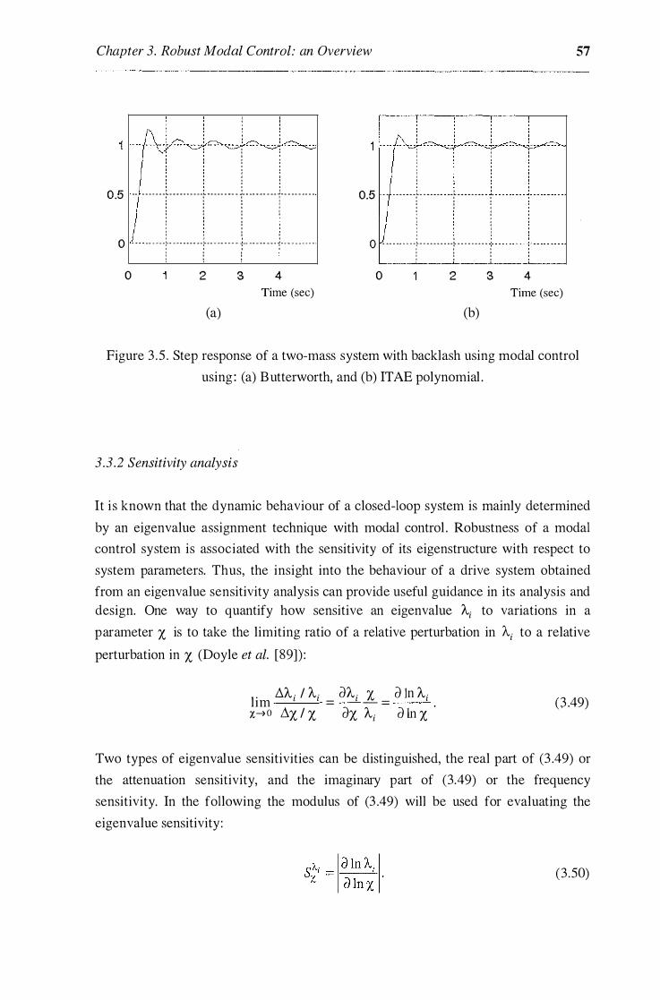
Chapter 3. Robust Modal Control: an Overview
- - - :� ----
0 5 I I I I · -- - - - - - - -r- - - - - - - - - -r · · - - - - - - - y - -- - - - - - -r- - - - - -- - -
• I I I I I I I ' ' ' ' ' ' ' ' ' ' I I I I 0 H - - - -- 0 - -+- - -- - - - - --�-- - - - - - - H +- - - - - - - - - �-- - - - - - - - -
0 ' ' ' ' ' ' ' ' '
2 3
(a)
4 Time (sec)
0.5 - - _ _ _ _ _ _ _ !" _ _ _ _ _ _ __ ! _ _ _ _ _ _ _ _ _
0 - - - - -- - - - -t- - - - - - - - - -t - - - - - - - - -
0 2 3
(b)
57
4 Time (sec)
Figure 3 .5 . Step response of a two-mass system with backlash using modal control using : (a) Butterworth, and (b) ITAE polynomial .
3.3.2 Sensitivity analysis
It is known that the dynamic behaviour of a closed-loop system is mainly determined by an eigenvalue assignment technique with modal control . Robustness of a modal control system is associated with the sensitivity of its eigenstructure with respect to system parameters. Thus, the insight into the behaviour of a drive system obtained from an eigenvalue sensitivity analysis can provide useful guidance in its analysis and design. One way to quantify how sensitive an eigenvalue 'Ai to variations in a parameter X is to take the limiting ratio of a relative perturbation in Ai to a relative perturbation in X (Doyle et al. [89]) :
lim !J.'Ai I 'Ai =
aA.i _z_ =
a ln 'Ai . x�o tJ.x I X ax 'Ai a ln X
(3 .49)
Two types of eigenvalue sensitivities can be distinguished, the real part of (3 .49) or the attenuation sensitivity, and the imaginary part of (3.49) or the frequency sensitivity. In the following the modulus of (3 .49) will be used for evaluating the eigenvalue sensitivity:
(3 .50)

Chapter 3. Robust Modal Control: an Overview 58
Using the right and left eigenvectors defined in (3 . 1 2) the eigenvalue sensitivities of a
high-order system can be evaluated by another way (Wu et al. [90]) :
(3 .5 1 )
where ui and v i are the right eigenvectors of the system matrix A , respectively.
Consider the position drive of Figure 3 . 1 . The plant dominant roots are found from the
characteristic equation (3 .39) in a general one-mass drive system:
or in the case of a DC drive:
'A = - -1 ( 1 ± � 1 - 4 7; J 1'2 2T T
' a m
(3.52)
(3 .53)
where all the parameters are specified in Section 3 .2. 1 . The sensitivity of the
dominant roots with respect to variations of the total moment of inertia can be derived
as following (Ha & Alferov [9 1 ]) :
"" () In A S1 = 1--- 1 m d in J,n
_!_[( 1mJ1cr )1/2 ± 1] 1 > 1 . 2 1m/ 1cr - 1 ' m cr (3 .54)
Figure 3 .6 plots the relationship between S} and 1cr jJ m . It is known that the system Ill
dominant roots are most sensitive to any variations of the moment of inertia around its
critical value Ucr/ 1m =1) . In some electrical drives of manipulators, the plant moment
of inertia 1m can be expressed as 1m = 10 + L\1 sin \f(t) . If the average value 10 lies in
the interval (0. 9 - 1 . 3 ) 1cr ' corresponding to s} 2 1 . 5 ' then the system dynamics is m
very sensitive to variations of load moment of inertia.

Chapter 3. Robust Modal Control: an Overview
4 .5 .-------,------.-----�,------.-------,------,
rn 0
·:c:J 4
· � •:c:J 3 .5
·� 3
s - 2 .5
§ 0 ·a
2 S"' at J /J < 1
8 1 .5
0.5
Jm m cr �
S"' at J /J > 1 Jm m cr
O L_--���--��-=====�==�
0 0 .5 0.9 1 1 .3 1 .5 2 2 .5 3
J /J m cr
Figure 3 .6. Dominant root sensitivities s; . 111
Similar remarks can be obtained with sensitivities S� and s£ : a a
59
(3 .55)
(3 .56)
These sensitivities are shown in Figure 3 .7 and 3 .8 . As it can be seen, within some
vicinity of critical values the dominant root sensitivities increase significantly.
As in the closed-loop case, it is known that in modal control, the system states are fed
back to the controller in order to assign the desired closed-loop eigenstructure and
thus, reduce its sensitivities . This is illustrated by the following sensitivity analysis for
the modal controller design using (3 .45).

Chapter 3. Robust Modal Control: an Overview
0 -� ·p · .-< [f) 5 [f)
0 8 § � l� 8
C/) <l)
·p .,.., :>
·p ..... (/] � <l) C/) ...... 0 0 !-< ...... § !=)
·s 0 0
4 .5
' I 4
3 .5
3
2 .5
2
1 .5 - - - -
1 - - - - - - - -/ · � - , - - - � - - - - - - - - - - - - - -
0 .5 // /'
0 /
/ '
0 0.5 0.83 1 1 .34 1 .5 2 2 .5 3
R /R a cr
Figure 3 .7 . Dominant root sensitivity S� . (/
4.5
4
3 .5
3
2.5
2
' 1 .5· - 1 ' - - - - - - - - � -J� - � -
, 1 0.5
·-------�-···/"� 0 -�··--····
0 0.5 0.75 1.13 1 .5 2 2 .5 3
L IL a cr
Figure 3 .8 . Dominant root sensitivities st . a
60
Equalising the coefficients ai ( i = 1 , 2 , 3 ) of the closed-loop characteristic polynomial
(3 .3 1 ) and of the desired one (i + 2800s + 0.6 )Cs + a3 - 280.0 ) gives:
(3 .57)
Chapter 3. Robust Modal Control: an Overview 61
where a1 = K1KcKpflm La , a2 = K/Kb + KcKv )/lm La , and a3 = (Ra + KcK1 )/La , and
00 and o are the dominant root frequency and damping factor, respectively. The
values of 00 and b , in practice, are affected by variations of plant parameters, e.g.
moment of inertia 1m and total resistance Ra of the armature circuit.
The differentials dQ0 and do can be obtained from (3 .57)
where
do = dO dR +
db dl dR
a d]
m ' a m
dO = d.Do dR +
d.Do dl 0 dR a
d] m
a m
db = 1 + 2b2 - oa3/00 dO _ _ [(a3/0.0 - 2b)2 - 1]b dRa OoLal!,. '
d]m
_d0_0 =
_ (a3 /00 - 2o) d0.0 = _ [(a3/00 - 2b)2 + 1 ]00 dl dRa La!!,. d]m ]ml!,. m'
(3 .58)
The sensitivities of dominant roots of the closed-loop system are then determined as :
It is inherent that infinitive sensitivities (3 .59) correspond to a multiple root the
characteristic equation with the binomial expansion criterion (a3=300 , o = 1). Since
s�o * 0 and sfo * 0 , a design with low sensitivities can be based on the conditions : a m
(3 .60a)
(3 .60b)

Chapter 3. Robust Modal Control: an Overview 62
Note that the condition (3.60a) at 8 =0.5 corresponds to the Butterworth (or magnitude
optimum) criterion. Using the dominant root-based modal controller (3 .45) the value
of coefficient a3 is determined from (3 .46):
(3 .6 1 )
Substituting the values of a3 given in (3.60a), (3.60b) and (3 .6 1 ) in (3.59) indicates
that the values of s�o and sfo at 0. 43 < 8 < 1 using the proposed dominant root-based a m
modal control (3 .6 1 ) are the least in comparison with the other techniques (3.60a) and
(3.60b) (Ha & Alferov [91 ] ) .
3.4 Combined observer for state and disturbance estimation
Modal control is capable of assigning the closed-loop eigenstructure for desired
transient performance. However, all states are assumed to be measured, whereas in
practice not all of them are accessible. Another problem with modal control is that
there is no guarantee for the control accuracy. Any external disturbance may result in
a steady state error. Combining state feedback with integral control can be a solution
to the problem, but it increases the degree of the system. An observer is required to
estimate the states and disturbance and thus, enables accomplishing feedback from all
the states and providing a feedforward compensation for the disturbance.
3.4. 1 Combined observer
This section is devoted to the design of a combined observer or a subsystem that
performs the observation of not only the state variables but also the external unknown
inputs based on information received from the measurements of the input and output.
The observer is implemented in a flexible system to estimate the elastic or reaction
torque, load speed as well as a load torque disturbance.
Consider the linearised model (3 . 1 ) . Assuming that the system can be written in a
partitioned form as
(3 .62)
y(t) = Cx(t) = ( Im O)x(t) = x 1 (t) ,

Chapter 3. Robust Modal Control: an Overview 63
where x1 (t) E Rm is the vector of measurable state variables, x2 (t) E Rn-m is the
vector of inaccessible state variables; AiJ • B i , and Di , i, j == 1 , 2 , are matrices of
appropriate dimensions; and the pair (C, A ) is observable. The problem is to
construct an observer for estimating both the state x2 (t) and the disturbance
v(t) E Rq .
Designing observers for recovering all the states of linear systems with unknown
inputs has attracted much research in the last few decades. State variables in general
can be estimated on the basis of a full-order or reduced-order Luenberger observer
[92] with known inputs. For state estimation in the unknown input case, some a priori information about the inputs is assumed in Meditch & Hostetter [93] . An existence
condition for a minimal-order observer, shown in Kudva et al. [94], is that
rank(CD) = q with q :S: m . (3 .63)
A necessary and sufficient condition for a full-order unknown input observer with a
direct design procedure is provided in Yang & Wilde [95] . A simple approach for
designing a reduced-order observer without any knowledge of the inputs is proposed
in Guan & Saif [96] . Other attempts focus on the estimation of not only state variables
but also unknown inputs. In Park & Stein [97], the state equation is transformed
through some substitutions into a special system model for a reduced-order observer
to simultaneously estimate states and unknown inputs. The problem of designing
observers for systems with unknown inputs is shown equivalent to that for
conventional unknown input free reduced-order systems, using a special descriptor
form in Hou & Muller [98] . On a practical standpoint, the design procedure in Alferov
& Ha [73] is straightforward with the introduction of a predictive coefficient to
approximate the unknown input rate of change. The idea behind this approach is to
augment the state equation of (3 .38) with an equation approximately describing the
dynamics of the external inputs (Kuzovkov [68], Meditch & Hostetter [88]):
v(t) = rv(t) ,
where r E Rqxq . The state model (3.8) can be written as :
(X I ) -(X') -. = A + Bu,
w w
(3 .64)
(3.65)

Chapter 3. Robust Modal Control: an Overview 64
where w == (x2 v l is to be estimated, A == [A1 1 A12J , B == (B1 ) , and C == (lm 0) A21 A22 B2
. - - ( ) - - (A21 J - (A22 D2 J w1th Al l = A1 1 , A1 2 == A1 2 D1 , B1 = B1 , A21 = O
, A22 = O
r , and
B2 = (:'} For the system (3 .4 1 ) a Luenberger observer exists if the pair ( C A) is
observable, i.e. if
(3 .66)
The pair (A1 2 A22 ) i s then also observable and a reduced-order observer can be
constructed (Luenberger [92]) :
z(t) == Fz(t) + Gy(t) + Hu(t) w(t) == z(t) + Ly(t)
(3 .67)
where z(t) E Rn-m+q is the observer state, w(t) = (x2 vl is the estimate of w(t) . The
observer matrices are determined as
(3.68)
where the observer matrix gain L = (�: ) , with L1 E R<•-m)xm and L2 E Rqxm , is
chosen according to the eigenvalue assignment of the observer characteristic equation:
lsin-m+q - F i == 0 . (3.69)

Chapter 3. Robust Modal Control: an Overview 65
The observer eigenvalues, which determine how fast the estimates converge to their
actual, should be located in such a way that the observer responds at least four or five
times faster than the closed loop system with a modal controller. If the external
disturbances v(t) are slowly varying, the matrix f' in (3.64) can be set equal to 0 . However, in many cases, v(t) may be arbitrary functions of time. Taking account of
time derivatives of disturbances till the (N - 1) -th order, v(t) can be approximated by
(3 .70)
where v�) is the i - th time derivative of v(t) at some t = t0 , i = 1 , 2, . . . , N - 1 , and
vCN) (t) = 0 . An observer of the order n - m + Nq can be constructed on the basis of T
the augmented state model (3.4 1 ) to estimate vector w(t) = (x2 v v0) . . . vCN-l ) v(N) ) with (Ha [9]) :
A1 1 A1 2 D1 0 . . . 0 0 Bl
Az1 Azz Dz 0 . . . 0 0 Bz 0 0 0 Iq . . . 0 0 0 A = B = , and C = (Im 0 0 . . . o o) . '
0 0 0 0 . . . 0 Iq 0 0 0 0 0 . . . 0 0 0 Such an observer can give better estimates of the unknown input dynamics, however
an increase in the observer order causes an adverse effect of lower reliability and
makes the system more sensitive to measurement noises. As an alternative to the
problem, a digital predictive observer is described in the next section.
3.4. 2 Digital predictive observer
Consider the linearised state model (3.28). The partitioned form as in (3.62) is written
in the discrete-time form as:
(3.7 1 )
y(k) = Cx(k) = (Im O)x(k) = x1 (k) ,

Chapter 3. Robust Modal Control: an Overview 66
The idea of a combined observer can be implemented by augmenting the state
equation with an equation modelling the disturbances v(k) by suitably chosen
dynamics. By introducing the derivatives v0) (k), v(2) (k) , . . . , vCN) (k) , the external
disturbances at the (k+ 1 )-th sampling point can be expressed as:
y2 TN v(k + 1) = v(k) + v0) (k)T + vC2) (k)-+ . . . +v(N)(k)-, (3 .72)
2 N !
where T is the sampling period. The state equation of (3. 7 1 ) is then written in the
augmented form:
All A1 2 Dl 0 0 x 1 (k + 1) A21 A22 D2 0 0 x1 (k) Bl x2 (k + 1) TN x2 (k) B2 v(k + 1) 0 0 I q IqT I - v(k) q
N ! 0 v0) (k + 1)
=
T(N-1 ) vC0 (k) + u(k). (3. 73) 0 0 0 0 Iq I q (N - 1 ) !
v(N) (k + 1) v<N) (k) 0 0 0 0 0 Iq
In order to avoid a considerable increase in the observer dimension when using the
augmented form (3 .73), a predictive approximation for v(k + 1) was proposed in
Alferov & Ha [73] :
v(k + 1 ) := (Iq + r)v(k) - rv(k - 1) , (3 .74)
where r = diag(yii ) is the diagonal matrix of predictive coefficients 'Yii E (- 1 , 1) , i = 1 , 2, . . . , q . The augmented form for the state model (3.28) using (3.74) is obtained
as :
(3 .75)

Chapter 3. Robust Modal Control: an Overview (x 1 (k) J y(k) = (Im 0 0) x2 (k) = x 1 (k) , v(k)
67
If system (3 .75) is observable, estimates for v(k) can be obtained from a reduced
order Luenberger on the basis of measurements x 1 (k) , the control signals u(k) and
the previous estimates v(k - 1) :
where
(3.76b)
and where z1 (k) E Rn-m and z2 (k) E Rq are observer state variables, L1 E rR(n-m)xm
and L2 E (Rqxm are observer matrix gains, x2 (k) gains, x2 and v are the estimates of
x2 and v . By denoting the estimation error vectors ex (k) = x2 (k) - x2 (k) , e v (k) = v(k) - v(k) , e = (ex ev f and using (3.76) , we obtain the following error
dynamics
(F1 1 F1 2 ) (0 0 ) e(k + l) = Fe(k) + F1e(k - 1) = e(k) + e(k - 1) . F21 F22 0 - r (3 .77)
The entries lu and Yu of matrices L1 , L2 and r , in general, are chosen by the desired
dynamic conditions of the observer according to the root assignment of the
characteristic equation
(3 .78)
The number (n - m) X m + (q x m) + m of chosen elements liJ , Yu is always greater
than the degree (q + m) of (3.78). Therefore, for given coefficients Yu = "fu0 , there
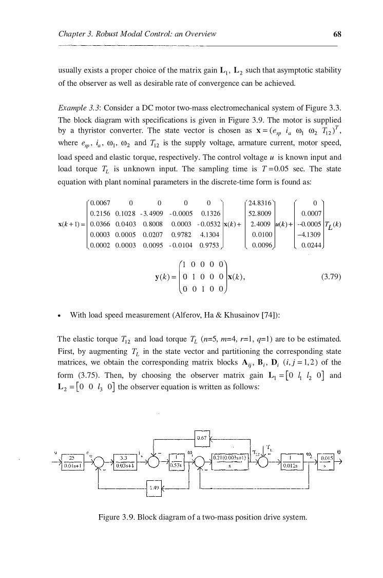
Chapter 3. Robust Modal Control: an Overview 68
usually exists a proper choice of the matrix gain L1 , L2 such that asymptotic stability
of the observer as well as desirable rate of convergence can be achieved.
Example 3. 3: Consider a DC motor two-mass electromechanical system of Figure 3 .3 .
The block diagram with specifications is given in Figure 3 .9 . The motor is supplied by a thyristor converter. The state vector is chosen as x == (esp ia co1 co2 � 2 )T ,
where esp , ia , co1 , C02 and �2 is the supply voltage, armature current, motor speed,
load speed and elastic torque, respectively. The control voltage u is known input and
load torque TL is unknown input. The sampling time is T ==0.05 sec. The state
equation with plant nominal parameters in the discrete-time form is found as:
0. 0067 0 0. 2 1 56 0. 102 8
x(k + 1 ) = 0. 0366 0. 0403 0. 0003 0. 0005 0. 0002 0. 0003
0 0 0 - 3. 4909 - 0. 0005 0. 1 326 0. 8008 0. 0003 - 0.0532 x(k) + 0. 0207 0. 9782 4. 1 304 0. 0095 - 0. 0 1 04 0. 9753 (I 0 0
y(k) = � 1 0 0 1
0 OJ 0 0 x(k) ,
0 0
24. 83 1 6 52. 8009 2. 4009 u(k) + 0. 0 100 0. 0096
.. With load speed measurement (Alferov, Ha & Khusainov [74]) :
0 0. 0007
-0. 0005 TL(k) -4. 1 309
0. 0244
(3 .79)
The elastic torque �2 and load torque TL (n=5, m=4, r=l , q= l ) are to be estimated.
First, by augmenting TL in the state vector and partitioning the corresponding state
matrices, we obtain the corresponding matrix blocks Aij • Bi , Di ( i, j = 1 , 2 ) of the
form (3 . 7 5) . Then, by choosing the observer matrix gain L1 = [ 0 11 12 0 J and
L2 = [ 0 0 !3 0 J the observer equation is written as follows:
Figure 3 . 9. Block diagram of a two-mass position drive system.

Chapter 3. Robust Modal Control: an Overview
z1 (k + 1 ) = J; 1z1 (k) + J;2z2 (k) + g11 e�P (k) + g12ia (k)
+ g1 3ro i (k) + g1 4ffi2 (k) + hlu(k),
Z2 (k + 1 ) = f21 Z1 (k) + fnZ2 (k) + g2Iesp (k) + g22ia (k) A
+ g23ro1 (k) + g24ro2 (k) + h2u(k) - YfL (k - 1), A A
� 2 ( k) = Z 1 ( k ) + 11 i a ( k) + 12 (J) 1 ( k) , TL ( k) = z2 ( k) + 13 (J) 1 ( k) ,
69
where z1 (k) , z2 (k) are the observer state variables, and the coefficients
f1 , gil , hi (i , j = 1 , 2, 1 = 1 , 2 , 3, 4) are calculated from (3 .76b) . The observer
characteristic equation is found to be:
For a given predictive coefficient y = y 0 , the elements l1 , 12 , l3 can be determined
from the desired observer pole assignment. For example, the deadbeat condition
gives:
where aij , di (i, j = 1 , 2, . . . , 5) are the matrix entries of the discrete-time state model
(3 .79) at nominal parameters of the system.
• Without load speed measurement (Ha [39]) :
The load speed ro2 , elastic torque �2 and load torque TL will be estimated (n=5 , m=3, r= l , q= l ) . By partitioning the state matrices into the form (3.76a) and choosing the
observer gain L1 = and L2 = [ 0 l5 16 ] , the observer equation can be [0 ll l2 ] 0 l3 14
written as follows:
z1 (k + 1) = J; 1z1 (k) + J;2z2 (k) + /13z3 (k) + g1 1esp (k)
+ g12ia (k) + g1 3ro1 (k) + h1u(k)
Z2 (k + 1) = f2 1z1 (k) + f22Z2 (k) + f23Z3 (k) + g2lesp (k)
+ g22ia (k) + g23 (J)l (k) + �u(k)
z3 (k + 1) = 1J 1z1 (k) + h2z2 (k) + h3z3 (k) + g3 1esp (k)
A
+ g32ia (k) + g33ffi 1 (k) + �u(k) - YfL (k - 1)

Chapter 3. Robust Modal Control: an Overview 70 W 2 ( k) = Z 1 ( k) + /I i a ( k) + /2 ffi 1 ( k)
A 112 (k) = z2 (k) + l3 ia (k) + Z4ro 1 (k) A
TL (k) = w(k) + l5ia (k) + Z6ro1 (k),
where z1 (k), z2 (k) and z3 (k) are the observer state, .�j , gu , and hi (i, j = 1 , 2, 3) are
coefficients calculated from (3.76b). The observer characteristic equation is found to be z4
+ a4z3 + a3z
2 + a2z + a1 = 0 , where
a! = 'Y(fufn - 1�2!21) , a2 = fuf23h2 + !221�3!1 1 + h3fi2f21 - h3f12f21 - ./�2./�d31 - !1 1!22!13 - Y(iJ 1 + !22) , a3 = .h dn + .f�2h3 + f33h 1 -
1�2!21 - ft3!1 1 - f23h2 + 'Y , a4 = -(ftl + !22 + !33) .
For a given coefficient y = y 0 , a solution for the observer deadbeat condition can be
obtained as follows:
with
l! = (a44a35 - a45a34) I ill ' l2 = (a24a45 - a25a44) I ill , l3 = (a54a35 - a55a34) I ill ' l4 = (a24a55 - a25a54) I ill ' ls = -( 'Y od3 + ( 1 + 'Yo )Cfi3a34 + f23a35)) I il2 , l6 = (y od2 + ( 1 + 'Yo K!;_3a24 + f23a25 )) I il2
!13 = d4 - lld2 - l2d3 , !23 = ds - l3d2 - l4d3 , ill= a24a35 - a25a34 , il2 = C.h_3a24 + f23a2s)d3 - Cft3a34 + f23a35)d2 ,
where the matrix elements au , di (i , j = 1, 2, . . . , 5) found in the discrete-time state
equation (3.79).
With the predictive coefficient chosen at y 0=0.5 and the observer gains are chosen to
meet the deadbeat condition, the actual and estimated load torque responses when TL
varies stepwise and sinusoidally are shown in Figure 3. 10. Note that for the /ak6 of
simulation, the observer initial state variables are set at ( 1 , 1 ) . The result indicates that
the proposed digital predictive observer with a well-chosen predictive coefficient can
provide correct estimates of not only plant's inaccessible state variables but also an
unknown load torque.

Chapter 3. Robust Modal Control: an Overview
1 .2 ,-----.----.----.-------,
0 .8 E g 0.6 1-� 0.4 1-
0.2
0 1'---------"'
- - - - - - - - - - - -r--�
-0 .2 L__ ___ L.__ __ ,____ __ ,____ _ ____J 0 50 1 00
time. x 0.05sec (a)
1 50 200
0.8
0.6 E 0
� 0.4 "" ...J 1-
0.2
0 ·
-0.2 0 50 1 00 1 50 200 time. x 0.05sec
(b)
Figure 3 . 10 . Actual and estimated load torque: (a) stepwise, and (b) sinusoidal.
3.5 Observer-based feedforward compensation
71
In high performance servo drive applications, control accuracy, fast response and
insensitivity to any perturbations are increasingly important requirements. Load
torque changes, parameter variation and nonlinear friction in servo systems are the
main cause of speed fluctuation and may result in unacceptable motion error. Any
variation in the motor generating torque, moment of inertia, or friction can be
considered as equivalent to an uncertain load torque change (Dote [65]) . Estimating
load torque as an unknown input to a drive system becomes of interest for its
monitoring and control . Load rejection for improving accuracy and system robustness
can then be accomplished by feedforward compensation from the estimated load
torque (Ohishi et al. [99], Ko et al. [78], Ha & Alferov [ 19]) , where the feedforward
gain is chosen from the zero steady-state error condition. In Schmidt & Lorenz [ 100] ,
load induced motion error is reduced by acceleration feedback with the acceleration
signal derived from a position signal via an observer. The acceleration signal can be
evaluated by using knowledge of the estimated load torque (Hori et al. [64]) . In this
section, the feedforward control principles are introduced to compensate for the load
torque influence using a disturbance observer.
Consider a linearised system with a continuous-time state model (3 . 1 ) or a discrete
time one (3.28). The key idea behind feedforward control here is to provide in addition to the modal control signal um (3 . 1 5b) or (3 .29) a compensation signal uf , which depends on the estimated disturbance obtained from an observer:

Chapter 3. Robust Modal Control: an Overview 72
u.t = K 1v , (3. 80)
where Kf E Rrxq is the matrix of feedforward coefficients . Since modal control, in
general, does not guarantee steady-state performance, the entries of K1 can be chosen
based on zero steady-state error conditions . In the following, we assume that q = 1 and
a load torque TL is considered as disturbance in drive systems with linearised models
(3 .2)-(3 . 5).
The schematic of a typical modal controller with feedforward compensation for a DC
motor drive of Figure 3 . 1 is shown in Figure 3 . 1 1 , where LTO is a load torque
observer. When the load torque TL is constant or slowly time-varying, the feedforward
gain Kf determined from the condition of zero steady-state error (the motor speed
co=O, current ia = TL/ K1 , supply voltage evp = TLRa/ K1 , control voltage
u = TLRa j K1 Ksp , and error ess = 0 ) is
(3. 8 1 )
where Ra and K1 are the motor armature resistance and torque constant, Ksp is the
supply amplifier gain, Kes and Kia are the supply voltage and current feedback gains .
L_ _ _ _ _ _ _ __ _ _ __ _ _ _ _
Figure 3 . 1 1 . State feedback and feedforward controller.

Chapter 3. Robust Modal Control: an Overview 73 For the case of a two-mass servo drive (Figure 3.2) using a DC motor, the controller
block diagram has the form of Figure 3 . 1 2. The zero steady-state condition requires the motor and load speed ro1 = ro2 = 0, elastic torque Te = TL , current ia = TL/ K1 , supply voltage esp = TLRa / K1 , control voltage u = TLRa / K1 Ksp ' and error ess = 0 . The feedforward coefficient is found in the same way:
where Kr12 is the elastic torque feedback gain.
(3.82)
Figure 3 . 1 2. Feedforward controller block diagram for a two-mass position drive.
Example 3.4 (Alferov & Ha [75]) : Consider the one-mass system of Example 3 . 1 .
Obviously, a steady-state error due to a load torque disturbance still exists even with
the use of a dominant root-based modal controller, as shown in Figure 3.2 . With the
feedforward gain obtained from (3 . 8 1 ), load torque influence can be completely
rejected as shown in Figure 3 . 1 3 for the one-mass system case.
Example 3.5: Consider the two-mass system of Example 3 .2. Figure 3 . 14 plots the
dominant root-based modal control step response with a load torque disturbance
exerted on a two-mass system at t = 3 sec with and without feedforward
compensation. As it can be seen in Figure 3 . 14(b) , the influence of a load torque is
quickly alleviated.

Chapter 3. Robust Modal Control: an Overview
0 .8 - - - - -0 - - - - - - -·- - - - - - - - -
0 .6 - - - - - - -:- - - - - - - - -0 .4 - - - - - - - -� - - - - - - - - -
0.2 - - - - - - - -·- - - - - - - - -
0 - - - - - - - - �- - - - - - - - -
0. 8 o. e
0.2 0
74
0 0.5 1 1 .5 2 0 0 .5 1 .5 2 Time (sec) Time (sec)
(a) (b)
Figure 3. 13 . Step response of an one-mass system with a load torque at t = 1 sec using
feedforward signal in : (a) dominant root-based, and (b) Butterworth pole placement.
- - - - - - - - - - - -'-"'· -�- �.;_-----.;.._ .. . . . . . . .. , . . . . . . .. . .
0.5 - - - - - - -+ - - - - - - --r· - - - - - ·-r · · - - - - --r - - - - - - - -
1 1 ' ' o - - - - - - - - -r · - - - - - --r -- - - - - - --r · - - - - - --r - - - - - - - -
0 2 3 4 Time (sec)
(a)
' ' 0 5 I I I I .
· · · · · · r · · ·r · · · r · · · · " · · · ·
0 - - - - - - - - - "!" - - - - - - - --:-- - -- - - - - i• - -- - - - - - - i-- - - - - - - - -0 2
(b)
3 4 Time (sec)
Figure 3 . 14. Step response of an two-mass system with a load torque at t = 3 sec ,
using dominant root�based modal control: (a) without compensation,
and (b) with feedforward compensation.
The results obtained indicate that observer-based feedforward compensation is a good
approach to the problem of load rejection in electromechanical systems. A main
disadvantage of the observer-based modal control is that the feedback and
feedforward controllers require correct knowledge of the plant parameters . Thus,
parameter sensitivity is a problem of this technique. Issues about robustness against
parameter variations will be discussed in the next section and in Chapters 5, 6, and 7.

Chapter 3. Robust Modal Control: an Overview 75 3.6 Robust modal control
For improving robustness in servo drives, several control techniques are evolving
such as the sliding mode in variable structure systems (Chang et al. [ 1 0 1 ]), self-tuning
and model reference adaptive controls (Bortsov et al. [87], Egami et al. [ 1 02]) . Sliding mode control i s efficient dealing with structured uncertainty such as changing
parameters and load. However, the observation noise and the chattering phenomena
due to large control gains are challenging issues and there is a trade-off between
robustness and chattering. Conventional adaptive control adaptive control algorithms
are usually complicated and thus, need excessive computation effort for real-time
implementation. Modal controllers, in general, are designed depending on an accurate
linearised model of the controlled system. In electromechanical systems, design
equations of modal control (3 .43), (3 .45) or (3 .48), and of feedforward control (3 . 8 1 ) or (3.82) indicate explicitly the relationship between the controller's and plant's
parameters . In order to obtain satisfactory control performance, the dynamics of
controlled systems are assumed to be known so that any control strategy can be
successfully applied. However, when the structure of the plant is unknown , and the
parameter variation is excessive, the effectiveness of modal control diminishes. Here,
in order to obtain parameter-insensitivity a robust control signal is added to the modal
control signal. Thus, the control signal consists of three components : the modal control signal um (t) , the feedforward control signal uf (t) , and the robust feedback
signal ur (t) . Such a controller is called a robust modal controller in Ha [9] . Design
procedures for continuous-time and discrete-time robust modal controllers are given
in this section. The asymptotic stability of the overall system is guaranteed by using
the second method of Lyapunov. Simulation results for one-mass and two-mass servo
systems are given to verify the validity of the proposed method.
3.6. 1 . Continuous-time robust modal controller
The design procedure starts with the assumption that the influence of external disturbances v(t) has been alleviated by the compensation signal uf (t) and then, the
single input ( r = 1) linearised model (3 . 1 ) with structured uncertainty can be brought
into the form:
(3.83)
y(t) = C0x(t) ,

Chapter 3. Robust Modal Control: an Overview 76 where A0 , b0 , and C0 are the nominal system matrices, and L).A and L).b are the
system uncertainties. The triple (A0 , b0 , C0) is assumed controllable and observable.
The principles of robust modal control are illustrated by a block diagram shown in
Figure 3 . 1 5 . A combined state-disturbance observer (SDO) as described in Section 3 .4
is used for evaluating the physically inaccessible state x2 (t) and the unknown
disturbances v(t) . The modal controller (MC) then accomplishes feedback from the
output y(t) = xl (t) and the estimated state x2 (t) :
(3. 84)
where Ur�f is the reference input, defining the steady state component. Considering
the transient response, the reference Ur�f is set equal to 0. Neglecting the observer
error, the modal signal (3 .84) has the form of (3. 1 5b). In order to deal with
uncertainties, the robust controller (RC) employs an additional robust feedback signal
ur (t) which will be determined in the following discussion. The feedforward
controller (FC) provides the compensation signal uf (t) (3. 80) for eliminating the
external disturbance influence, hence v(t) can be omitted in the state equation (3 .83).
Substituting (3. 1 5b) and the robust feedback signal ur (t) into (3 . 83) gives :
where E(t) E Rn is an infinitesimal vector due to the observer error and incomplete
compensation. Denoting Am = A0 - b0kT and L).Am = L).A - L).bkT , and neglecting
E(t) , (3. 85) becomes:
I qefl
I I I I I I I I _ ··- - - - - - - - - - - - _j
v
Plant
Figure 3 . 1 5 . Robust modal control block diagram.

Chapter 3. Robust Modal Control: an Overview 77
(3 .86)
The following assumptions are made (Jabbari & Schmitendorf [ 1 03]):
A 1 . The uncertainties are continuous matrix functions of the vector of varying system
parameters p E IP c RP , where IP is a compact set:
(3.87)
A2. There exist a vector r(p) E Rn and a scalar s(p) such that (matching conditions):
L\.b = b0h(p) and Jh(p) J � cr < 1, Vp E IP ,
where I I . II denotes the Euclidean norm.
Theorem 3.2 (Ha [9])
(3 .88)
Consider the continuous-time system (3.86) satisfying the assumptions A l and A2,
given in (3 .87) and (3 .88). For any positive-definite matrix Q and positive scalar y r satisfying:
where A-min (Q) is the minimum eigenvalue of Q , the control law
(3 . 89)
(3.90)
is a robust stabilising control with the robust feedback gain kr = "{ rPb0 , where P is
the solution of the Lyapunov equation:
(3 .91)
Proof Choose a Lyapunov function candidature of the form V(x) = xT (t)Px (t) , where P is a unique positive-definite solution of (3 .91) . The trajectory time derivative
is obtained using (3 . 86) and (3.90):
Chapter 3. Robust Modal Control: an Overview 78 V(x) = xTPx + xTPx =
T T T T -= [x (Am + �Am ) + ur (b0 + �b) ]Px + X P[(Am + �Am )x + (b0 + �b)ur ] = . T T T T T V(x) = X [AmP + PAm + �AmP + P�Am - 2y rPb0b0P - 2y rh(p)Pb0b0P]x = xTL(p)x,
where L(p) = - Q + r(p)b�'p + Pb0rT (p) - 2yr (l + h(p))Pb0b�'p .
Applying to the above equation the following identity xxr + yyT :2: XYT + YXT for
n x m -matrices X and Y gives:
1 L(p) � - Q + rrr - y r (2 + 2h(p) - -)Pb0b�P . 'Yr
If the coefficient y r is chosen such that y r :2: 1 , then
2(1 + h(p))
Since sup 1 = -1- and sup jjr(p) j j = p , the derivative of the Lyapunov function
pEOo 1 + h(p) 1 - 0' pEIP is negative definite if Q and y r are chosen satisfying (3 .89). This concludes the
proof.
Example 3.6: Consider Example 3.2 with the two-mass system of Figure 3 .3 . Assume
that the dynamic stiffness of the drive speed-torque characteristics is an uncertain
parameter with a variation of 50% of its nominal value. The state model (3.5) can be
obtained as
Tm -33. 3 - a 0 0 Tm a 0 0)1 1 . 23 0 1. 23 0 cot 0 0
= + cor�f' + TL 112 0 0. 2 1 0 - 0. 2 1 112 0 0 0)2 0 0 83. 3 0 C02 0 -83. 3
where a = 237 .3 ± 1 1 8 . 7 . The dominant root-based method gives the state feedback gain kr = [0. 037 1 1 . 2 1 87 63. 96 0. 1 863] . With (M)1 ,2 = (�B)1 = 1 1 8 .7 and
(M\Jo;tl,2 = (�B)i-pl = 0 , the rows of �Am are found to be (Mm )i-pt = [0 0 0 0] and
(Mm ) 1 = -10-2 [0. 02 0. 1 1 3 1. 98 0. 09] . Thus, the bounds p and cr are determined
as 0.32 and 0.5, respectively. From the solution of the Lyapunov equation (3 .91) , the

Chapter 3. Robust Modal Control: an Overview 79 robust feedback gain according to (3.90) is calculated as k; = [ -0. 1 0 . 0004 0. 03 0 . 002] . The step response of the load speed with a 50%
reduction in the dynamic stiffness (a = 1 1 8 . 7 ) without robust feedback is shown in
Figure 3 . 1 6(a), and with robust feedback in Figure 3 . 1 6(b) where an improvement of
transient performance is observed. The influence of backlash nonlinearity with a
deadband width of 2D = 0. 02 in the coupling shaft gear is considered in Figure 3 . 1 7 .
It is indicated that an additional robust feedback (Figure 3 . 17 (b)) helps increasing
robustness against unstructured uncertainty such as backlash nonlinearity.
- -- - -- - --··- -·.,.- _.,.;._ _ __;.. __ .;__-l
. ' 0 5
I I I I · - -- - - - - - - r - · ·- - -- - ·· r -- - - - - - - - ;- - -- - -- - -- � - - - - - - - - - -. ' ' ' ' ' ' ' '
I I I I
0 - - - - -- - - -+- - - - - - - - -+ -- - -- - - - - + - - - - - - - - - �- - - - - - - - - -
0
' ' ' ' ' '
2 3 4 Time (sec)
(a)
0 1 2 3 4 Time (sec)
(b)
Figure 3 . 1 2 . Step response of the load speed with a 50% reduction in the dynamic
stiffness: (a) without robust feedback, and (b) with robust feedback.
0.5
' ' ' ' - -- - -- - - - -.- - - - - -- - - - -- - --' ' -� --
I I I I - - - - - - -- . .. . - - - - - - - -- 1.. - - - - - - - - - ... - -- - - � - -- .. . - - - - - -- - -I I I I I I I I I I I I I I I I ' ' ' ' ' ' ' '
I I I I 0 - - - -- - -- -
:- - - - - -- - - -: -- - - - - - - - :- - -- - -- - -- :- - - - - - - - - -
0 1 2
(a)
3 4 Time (sec)
0 .5
- -- - - - - ---'f'""--:--�'7·=---=- -=· �----j
I I I I - - - _ _ _ _ _ _ .. _ _ __ _ _ _ _ __ .. _ _ _ _ _ _ _ _ _ _. _ _ _ _ _ _ _ _ _ _ ..� _ _ _ _ _ _ _ _ _ _ I I I I ' ' ' ' ' ' ' ' ' ' ' ' ' ' ' ' ' ' ' ' ' ' I I I I 0 -- - - - - - - -:- - - - - -- - - -: - - - -- - - - - :- - - - - -- - -- :- - - - - - - - - -
0
I I I I I I I I I I I I
2
(b)
3 4 Time (sec)
Figure 3 . 17 . Step response of the load speed with backlash 2D = 0. 02 : (a) without
robust feedback, and (b) with robust feedback.

Chapter 3. Robust Modal Control: an Overview 80 --------------------------------------------------------------
3. 6. 2. Discrete-time robust modal controller
Now consider the discrete-time case when the state model can be written as:
x(k + 1 ) = (A0 + �A)x(k) + (b0 + �b )(um (k) + ur (k) ) , (3.92)
y(k) = C0x(k) ,
where A0 , b0 , and C0 are the nominal system matrices, and �A and �b are the
system uncertainties for the model written in the discrete-time form. The triple (A0, b0 , C0 ) is assumed controllable and observable. It is also assumed that the influence
of external disturbances v(k) in the state model (3.28) has been compensated for with
the use of a feedforward signal uf ( k) . Following the schematic shown in Figure 3 . 1 1 ,
and again assuming a complete rejection of v(k) , the closed-loop dynamics with
discrete-time robust modal control can be described by:
(3 .93)
where Am = A0 - b0kr, �Am = �A - �bkT , and kT is the feedback gain of the
modal controller (MC). The determination of the robust controller (RC) is given in the
following theorem:
Theorem 3.3 (Alferov & Ha [36]) Consider the discrete-time system (3.93) satisfying the assumptions AI and A2, given
in (3 .87) and (3.88) . For any positive-definite matrix Q satisfying:
A min (Q) > b�Pbo (-p-) 2 = Acr ,
1 - (J (3 .94)
where Amin (Q) i s the minimum eigenvalue of matrix Q , and P is the solution of the
discrete-time Lyapunov equation:
(3.95)
the control law:

Chapter 3. Robust Modal Control: an Overview 81
(3 .96)
is a robust stabilising control.
Proof Define the scalar function h(k) = rT (p)x(k) + (1 + s(p))u,. (k) , the above state
equation (3 .93) can be rewritten as
S ince Am is stable, there exists a symmetric positive definite matrix P satisfying the
Lyapunov function (3.95) for any given symmetric positive definite matrix Q . Choose
a Lyapunov function candidature of the form V(x) = xT (k)Px(k) . The differential
change
L\ V(k) = V(k + 1) - V(k) = xT (k + l)Px(k + 1) - xT (k)Px(k) ,
can be expressed as
L\ V(k) = [Amx(k) + b0h(k)f P[Amx(k) + b0h(k)] - XT (k)P(k)x(k) = xT (k) [A�PAm - P]x(k) + h(k)[b�,Pb0h(k) + 2b�PAmx(k)]
L\ V(k) = -xT (k)Qx(k) + h(k)[y0h(k) + 2<p(k)],
where Yo = b�Pb0 is a positive constant, and <p(k) = b�PAmx(k) is a scalar function.
The quadratic form h (k)[y0h(k) + 2<p(k)] will be non-positive if h(k) lies in the
interval between 0 and -2<p(k)/cr . Under the control law:
2<p(k) --
+ PIIxCk)ll I I I I Yo -::;, u,. (k) -::;, -p x(k) , when <p(k) � 'YoP llx(k)l l l + cr 1 - cr 1 - cr
when <p(k) = 0
- 2<p(k) + Pllx(k)ll Pllx(k)ll -::;, u,. ( k) -::;, Yo
' when <p(k) -::;, - YoP llx(k)l l · 1 - cr 1 + cr 1 - cr

Chapter 3. Robust Modal Control: an Overview 82
the differential change ilV(k) has an upper bound given by (Yang & Tomizuka
[1 04]) :
Thus, if the condition (3 .94) is satisfied then the system will be asymptotical stable
under the control law above. By this control law, the robust feedback signal ur (k) should lie in the interval between
-2<p(k)/Y 0 + pj jx(k)jjsgn( <p(k)) and
-pjjx(k )jjsgn( <p(k )) 1 - (} 1 - ()
The problem is to determine two positive real numbers K 1 and K2 satisfying
K1 + K2 = 1 such that the resulting robust feedback signal
(k) _ -2<p(k )/Y 0 + pjjx(k )j jsgn( <p(k)) _-p:....!!jj_x(_k )'-"-jjs..:::..gn--'(_:_<p..:......(k.:_:_)) ur - Kl + Kz 1 - cr 1 - cr
can tolerate the largest uncertainty range, or have the simplest form. The latter leads
to the choice
l + cr 1 - cr K1 = -- and K2 = --2 2
by which the nonlinear term pj jx(k)jjsgn( <p(k)) can be omitted from the control signal
ur (k) . In that case, the robust feedback signal ur (k) is then obtained
This concludes the proof.
Example 3. 7 (Alferov & Ha [ 1 9 , 36]) : Consider the system of Figure 3 . 1 using the DC
motor of the type PGT-2 with the following specifications : Kc = 1 2 , I:: = 0. 007 sec , Ra = 0. 785ohm, La = 3.92mH , Bm = 0 , lm = 0. 002kgm2 , Kb = 0. 297Vs I rad and
K1 = 0. 297V I A . The sampling time is T = 0. 003 sec .

Chapter 3. Robust Modal Control: an Overview 83
The state feedback gain k T = [ K E K v K 1 K r J computed using the magnitude
optimum criterion is k T = [0.1 33 0.025 0.005 4.362] . Assume that the total inertia
and armature resistance vary in the intervals 1m E [1 , 2]1 m,nom and Ra E [1, l .2]Ra,nom·
From the uncertainty matrices �Am and �b of the form (3.93), the values of p , cr , and "Acr i s found to be 0 . 1 1 5 , 0. 1 7 , and 0.92, respectively. Choosing Q = I , the robust feedback gain k� = [ �KE �Kv �K1 �Kr J is obtained from (3.95) to be
k� = -[0.06 0.059 0.1 1 OJ .
The position step response with 1m = 21 m,nom and Ra = 1 . 2Ra,nom is plotted in Figure
3 . 1 8 . It is observed in Figure 3 . 1 8(b) that robustness of the system is significantly
improved with the use of an additional robust feedback gain transient.
Further comparison between the methods of assigning the closed-loop poles, the
inf1uence of parameter and load variations, and simulation and experimental results
were reported in Ha [9] and Ha & Alferov [75, 1 9, 36, 9 1 ] . The results verify that
robust modal control can be an efficient technique for vibration suppression, load
rejection with high robustness in electromechanical systems, especially systems with
flexible structures.
1 .5 ..----,----.----r---.----.
0 .5
' ' ' ' , - - - _ _ _ _ _ _ ._ _ _ _ _ _ _ _ _ _ _ �.. _ _ _ _ _ _ _ _ _ ' ' ' ' ,
� �- M -- � -� _. __ - -- - - - - -'
0 - - - - - - - - - -�- - - - - - - - - -� - - - - - - - - - - - - - - - - - - -:- - - - - - - - - -
0 0 . 1 0 .2 0 .3 0 .4
Time (sec)
(a)
' ' ' 0 .5 - - - - - - - - -:- - -- - - - - - -: -- - -- - - - - - - - - - W D N _ ... _ _ _ _ _ _ _ _ _ _
' ' ' ' '
0 - - - - - - - - - -�- - - - - - - - - -� - - - - - - - - - - - - - - - - - - -:-- - -- - - - - -
0 0 . 1 0 .2 0.3 0 . 4
Time (sec)
(b)
Figure 3 . 1 8 . Position step response with 1m = 21m,nom and Ra = 1 . 2Ra,nom :
(a) without robust feedback, and (b) with robust feedback.

Chapter 3. Robust Modal Control: an Overview 84
3.7 Summary
An overview of the robust modal control technique has been comprehensively
outlined in this chapter. It started with the mathematical description of linearised
models for some position drives and focused on the servo drives with flexible
structures . The methodology to construct a modal controller for these systems is
addressed, considering both continuous-time and discrete-time cases.
The first contribution of this chapter is the proposed dominant root-based technique
applied for one-mass and two-mass servo systems. The key idea here is that the
closed-loop system dynamics is decided mainly by the location of the dominant root
pair. Thus, when choosing the desired poles for determining the state feedback gain,
additional conditions relating to accuracy or damping capability can be taken into
consideration. This may remove the drawback that modal control cannot affect the
steady-state control performance, and relax the conservatism of Kukharenko's method
combining the equalising equations in modal control with control accuracy
requirements . Design equations for servo systems with maximum damping are
provided. Vibration suppression capability when the system is subject to backlash
nonlinearity is verified. Insight into robustness of servo systems with modal control is
provided by an eigenvalue sensitivity analysis. It is shown that in the vicinity of some
critical values of the drive parameters, the dominant root sensitivities increase
significantly. With the damping ratio lying between 0.43 and 1 , the dominant root
based technique provides some advantage over other standard assignment criteria in
terms of sensitivities.
As a matter of fact, not all the system state variables are physically available to be fed
back in modal control, hence, they need to be estimated. Moreover, unknown inputs
to the system also need to be evaluated for the compensation purpose. An interesting
part of this chapter is devoted to the design of a combined observer for
simultaneously estimating the system states and external disturbances, based on
measurements of the system input and output and some a priori information of the
unknown inputs . Such an observer can take into consideration the disturbance rate of
change. A digital predictive observer is constructed on the basis of an augmented
form of the state equation with an additional equation approximating the disturbance
dynamics. The proposed observer can be applied to estimate the torsional torque and
load speed, and load torque in a multi-mass servo system. Based on load torque

Chapter 3. Robust Modal Control: an Overview 85 estimates, feedforward compensation principles can be applied to reject the
disturbance influence. It is shown that with a properly chosen feedforward gain, any
deteriorations in servo performance due to load changes can be completely
compensated for.
Considering the parameter variation problem, a robust feedback signal is added to the
modal signal. The control signal then consists of three components: modal control
signal, feedforward compensation signal, and robust feedback signal. When the
matching conditions are satisfied, given the bounds of uncertain matrices of the state
model, the asymptotic stability condition can be determined via the second method of
Lyapunov. Design procedures for the continuous-time and discrete-time robust modal
controllers are illustrated in servo drive systems. Simulation results demonstrate the
system parameter- and load-insensitivity, and also robustness against nonlinear
phenomenon such as backlash in the coupling shaft gear of a two-mass servo system.
Although robust modal control is efficient for systems with flexible structures, the
observer and feedforward compensator are designed based on system nominal
parameters, and thus parametric robustness of the whole system has not completely
achieved. The followin g chapters will address this problem using artificial intelligent
tools such as fuzzy logic and neural network approaches.

Chapter 4
Fuzzy Logic and Fuzzy Logic Control
Fuzzy logic has been explored for over three decades and is currently the focus of
popular and technical press . The area of process and control engineering has attracted
much attention in fuzzy logic. This is explained by the salient advantage of fuzzy
logic as a valuable tool in the design of embedded machine intelligence. Yet control
systems exploit only a fraction of its representational power. Oriented toward
applications, it is believed that the tolerance for imprecision of fuzzy logic makes it
suitable to address the problems of robustness. As an introduction to the use of fuzzy
logic schemes to enhance robust performance of motion control systems, this chapter
briefly describes basic concepts about fuzzy logic and fuzzy logic control , and
outlines some current research to fuzzy control systems.
4.1 Introduction
Fuzzy logic is a method for representing information in a way that resembles natural
human communication, and for manipulating that information in a way that resembles
how humans reason with it. In the early 1 960s, Prof. Lotfi A. Zadeh, the inventor of
Fuzzy, began to feel that traditional systems analysis techniques were too precise for
real-world problems and a new technique, a "fuzzy" kind of mathematics, was needed
(Perry [ 1 05]) . That idea came to Zadeh in July 1964 and he published the first paper
on fuzzy sets in 1 965 [ 12] . Through over a decade after that seminal paper, fuzzy set
theory was raising controversial debates within academic community. Eventually,
fuzzy theory was taken seriously by the Japanese electronics companies with its
implementations in numerous of consumer products (dishwashers, washing machines,
air conditioners, cameras, microwave ovens, camcorders, and so on) . Since successful
applications of fuzzy logic ranging from consumer products to industrial process
control, medical instrumentation, decision-support system and portfolio selection
(Zadeh [ 106]), fuzzy logic has not only won a wide acceptance but also become hot

Chapter 4. Fuzzy Logic and Fuzzy Logic Control 87 ------------
topic with an explosion of l iterature on it: hundreds of books, thousands of technical
papers have been written on this subject.
Among diverse areas of fuzzy logic applications, control is the area to which fuzzy
systems are most widely applied today. The genesis of fuzzy logic control was a 1972 paper by Chang and Zadeh [ 1 3] outlining the basic approach. An important landmark
in this development was the introduction of the linguistic variables whose values are
linguistic terms rather than numbers (Zadeh [ 1 07]) . Fuzzy technology, Zadeh
explained, is a means of computing with words for which the role model is the human
ability to reason and make decisions without the use of numbers [ 1 08] . The first
implementation of these ideas was described in a paper by Mamdani in 1974 [ 1 09] . The key principle underlying fuzzy logic control is based on a logical model which
represents the thinking process that an operator might go through to control the
system manually. The viability of fuzzy logic control has been demonstrated through
wide-spread applications (Schwartz et al. [ 14]). Fuzzy logic control can be considered
as one of intelligent control techniques where engineering knowledge is reflected in
the controllers . It has been found that such controllers have definite advantage over
the traditional PID controllers in that they are more robust with respect to structured
and unstructured uncertainties. The linguistic characteristics of fuzzy control provide
a very good approach in order to account for the sensor noise, unmodelled dynamics,
parameter variation, disturbance influence and nonlinearities (Lee [ 1 1 0]) .
It is known that classical PID controllers do not work well for the case of nonlinear
control and, even for linear control they typically have to be redesigned according to a
new set of the basic system parameters. Adaptive controllers have been proposed for
these systems. By means of some tuning schemes, the controller parameters can be
continuously adjusted to improve robustness against any changing environment. Auto
tuning (Astrom et al. [ 1 6]) or auto-calibration (Voda & Landau [ 1 7]) of controllers for
plants with uncertainties is useful although some knowledge of the process is needed.
Tuning the controller parameters to achieve better performance can be accomplished
by means of fuzzy logic (Tseng & Hwang [20] , Ha & Negnevitsky [2 1 ]) . In Truong & Hofmann [ 1 1 1 ] , conventional controller parameters are modified during operation by
incorporated fuzzy tuners. Fuzzy tuning with explicit schemes has been proven to be
capable of enhancing robustness without increasing computational burden to the
controller (Ha [ 1 1 2], Ha & Negnevitsky [35]).

Chapter 4. Fuzzy Logic and Fuzzy Logic Control 88 Despite a large number of technical publications focusing on fuzzy systems, there
exists some doubtful opinion on fuzzy co11trollers mainly because of some
misunderstanding about fuzzy control. Attempts have been made to clear up this
misunderstanding, e.g. Jager [ 1 1 3] . It is, therefore, of interest to start the notable part
of this thesis, using fuzzy tool in combination with other techniques, with a short
prither bn fuzzy set theory, fuzzy reasoning, and fuzzy logic control.
4.2 Fuzzy set theory
There is a vast amount of literature on fuzzy logic. This literature is growing rapidly
in recent years, making it difficult to present a comprehensive survey of its wide
applications . A lot of it is too theoretical to be applied to engineering problems. The
purpose of this section is to briefly summarise the basic concepts that are necessary in
order to understand fuzzy logic and fuzzy inference from a practical viewpoint.
4.2 . 1 . Fuzzy sets (Mendel [ 1 1 4])
A universe of discourse U is the set of allowable values for a variable, denoted generically by { x} which could be discrete or continuous, where x represents the
generic element of U . A crisp set A in a universe of discourse U can be defined as A = {xi !!A (x)} , where
!! A (x) is, in general, a condition by which x E A . If we introduce a zero-one
characteristic function such that A :::::::> (!!A (x) = 1 if x E A and I-LA (x) = 0 if x E A) then
!! A (x) is called a membership function for A .
Afuzzy set F in a universe of discourse U is characterised by a membership function !!p (x) which takes on values in the interval [0, 1] . A fuzzy set is a generalisation of
an ordinary (i.e. crisp) set whose membership function only takes on two values {0, 1 } . A membership function for a fuzzy set F provides a measure of the degree of similarity of an element in U to F . A fuzzy set F in U may be represented as a set of
ordered pairs of a generic element x and its grade of membership function: F = {(x, !!x (x))l x E U} . When U is continuous, F can be written concisely as
F = fu 11 F (x) I x , where the integral sign denotes the collection of all points x E U with associated membership function 1-LF (x) . When U is discrete, F is represented as F = .2, u!! F ( x) I x, where the summation sign denotes the set theoretic operation
union. The slash in these expressions associates the elements in U with their

Chapter 4. Fuzzy Logic and Fuzzy Logic Control 89 membership grades, where J.!F (x) > 0 . Note that in fuzzy sets, an element can reside
in more than one set to different degrees of similarity . This cannot occur in a crisp set
theory.
The support of a fuzzy set F is the crisp set of all points x E U such that J.!F (x) > 0 .
The element x E U at which J.!F (x) = 0. 5 i s called the crossover point. For example,
the formal domain for normal weight might be 40 to 1 00 kg. However, the fuzzy sets
HEAVY and LIGHT can have non-zero membership grade at 50 to 90 kg with a
crossover point at 70 kg, as shown in Figure 4. 1 . A fuzzy set whose support is a single point x in U with J.L F (x) = 1 is called a singleton. In a singleton output space, fuzzy
set membership functions are represented as single vertical points. Figure 4.2
illustrates how a variable SPEED can be composed on individual single points.
�x) Degree of membership
1
, � crossover� point OL------=------�------�------� 40 50 70 90 100
, weight (kg) '
support <�------��------�
universe of discourse <------��������-------+
Figure 4. 1 . Fuzzy variable "weight" .
J.!(X) 1 . . . . . ............. . . . . . . . . . . . . . . . . . . . . . . . . . . . . . . . . . .. . . . . . . . . . . . . . . . . . . .
0 40 60
speed
80 (km/h)
Figure 4.2. S ingleton representation.

Chapter 4. Fuzzy Logic and Fuzzy Logic Control 90 A technical concept closely related to the support set is the alpha-level set or the
a - cut. An alpha level is a threshold restriction on the domain based on the
membership grade of each domain value. An a - cut contains all the domain values
that are part of the support at a minimum membership grade of a . There are two types of a -- cuts : weak and strong. The strong a - cut is defined as !J,p (x) :2: 0. 5 , and the
weak a - cut is indicated by !J,p(x) > 0. 5 . Thus, the strong 0 - cut defines the support
of a fuzzy set. Figure 4.3 depicts an 0 .2 - cut on the domain of fuzzy set HEAVY.
�x) Degree of membership
1 - - - - - - - -
0.5
0.2
weight (kg)
Figure 4.3. An a - cut for the fuzzy set HEAVY.
4. 2 .2 Set theoretic operations (Lee [ 1 1 0])
Let fuzzy sets A and B in U be described by their membership functions 1-1 A (x) and
1-1 B ( x ) . The set theoretic operations of union, intersection , and complement for fuzzy
sets are defined as following:
Union: The membership function of the union A u B is pointwise defined for all
X E U by
(4. 1 )
Intersection: The membership function of the intersection A n B is pointwise defined
for all x E U by
(4.2)

Chapter 4. Fuzzy Logic and Fuzzy Logic Control 91
Complement: The membership function of the complement of A is pointwise defined
for all x E U by
(4.3)
In order to model fuzzy union and fuzzy intersection other operators can be chosen. In
his pioneering first paper [ 1 2] , Zadeh defined maximum (4. 1 ) and algebraic sum
(4.4)
for fuzzy union, and minimum ( 4.2) and algebraic product
(4 . 5)
for fuzzy intersection. Later, based on axiomatic definitions (see, e.g. Yager & Filev
[ 1 1 5]) , general triangular conorm ( t - conorm or s -norm, denoted EB ) operators were
introduced for fuzzy union, and general triangular norm ( t - norm, denoted * )
operators for fuzzy intersection. Some other examples of t - conorms are bounded sum:
and drastic sum:
x EB y = min(1 , x + y) ,
{X if y = 0, X EB y = y if X = 0,
1 if x, y > 0.
Some other examples of t - norms are bounded product:
and drastic product:
x * y = max ( 0, x + y - 1 ) ,
{X if y = l ,
x* y = y �f x = 1 ,
0 1f x , y < 1.
(4.6)
(4.7)
(4.8)
(4.9)

Chapter 4. Fuzzy Logic and Fuzzy Logic Control 92 Although there are different operators, most engineering applications of fuzzy sets use
the minimum or algebraic product t - norm for fuzzy intersection, the max t - conorm
for fuzzy union and (4. 3 ) for the membership function of fuzzy complement (Mendel
[ 1 1 4]) .
Hint: Unlike crisp sets, the Law of Contradiction, A u A = U , and the Law of Excluded Middle, A n A = 0 , do not hold in fuzzy set theory, i .e. for fuzzy sets:
A u A :f:: U and A n A -::;:. 0 .
Cartesian product: If A1 , . . . , An are fuzzy sets in U1 , . . . , Un , respectively, the Cartesian
product of AI , . . . , An i s a fuzzy set in the product space ul X . . . x un with the
membership function
(4. 1 0a)
or (4. 10a)
Fuzzy relations: Fuzzy relations represent a degree of presence or absence of
association, interaction, or interconnection between the elements of two or more fuzzy sets. An n - ary fuzzy relation is a fuzzy set in U1 x . . . xUn and is expressed as
Compositions: Because fuzzy relations are fuzzy sets in the product space, set
theoretic and algebraic operations can be defined using operators for fuzzy union,
intersection and complement. Let R and S be fuzzy relations in U x V . The
intersection and union of R and S , which are compositions of the two relations, are
defined as
(4. 1 2a)
and
1-1 Ru S (X' Y) = !-! R (X' Y) EB !l s (X' Y) , (4. 1 2b)
respectively, where * is any t - norm, and EB is any t - conorm.
Next, consider the composition of fuzzy relations from different products spaces that
share a common set. If R and S are two fuzzy relations in U x V and V X W ,

Chapter 4. Fuzzy Logic and Fuzzy Logic Control 93 respectively, the sup-star composition of R ( U X V) and S (V X W) is a fuzzy relation
denoted by R o S ( U x W ) and is defined by
(4. 1 3)
where * could be any operator in the class of t - norm (the sup-min and sup-product
is most commonly used) . When U, V and W are discrete universe of discourse, the sup
operation is the maximum. Figure 4.4 depicts a block diagram for the sup-star
composition.
X E U )l �R(X,y) !r---_Y_E _V { �s(y,z) 1 -ZE� - - !lR>s(x,z)
R S
Figure 4.4. Block diagram interpretation for the sup-star composition.
Suppose fuzzy relation R is just a fuzzy set, then llR (x, y) becomes llR (x) and
V = U, consequently, sup[!lR (x, y)* !ls (y, z)] == sup[!lR (x)* !ls (x, z)] . Thus, when R yeV xeU
is just a fuzzy set, the membership function for R o S is
llRos (z) == suP[!lR (x)* !ls (x, z)] . xeU
(4. 14)
Figure 4.5 represents the block diagram interpretation for the sup-star composition
when the first relation is just a fuzzy set.
V= U
R
Figure 4.5 . Sup-star composition when V == U .

Chapter 4. Fuzzy Logic and Fuzzy Logic Control 94 4. 2. 3 Linguistic representation
A. Linguistic variables
The use of fuzzy sets provides a basis for a systematic way of for the management of
vague and imprecise concepts. According to Zadeh [1 16] , in retreating from precision
in the face of overpowering complexity, it is natural to explore the use of what might
be called linguistic variable, i .e. , variables whose values are not numbers but words or
sentences in a natural or artificial language. Fuzzy sets can be employed to represent
linguistic variable. Consider a real line as a continuous universe of discourse U . A
fuzzy number F in U is a fuzzy set which is normal and convex, i .e . ,
max llF (x) = 1 , (4. 1 5a) XEU
A linguistic variable can be regarded as a variable whose value is a fuzzy number or
whose values are defined in linguistic terms or labels. A linguistic variable is
characterised by its name u ; the term set of u , i.e., the set of terms T(u) of linguistic
values of u with each value being a fuzzy number defined on U ; a syntactic rule for
generating the names of values of u ; and a semantic rule for associating with each
value its meaning.
As an example, let SPEED ( u ) of a car be a linguistic variable. It can be decomposed
into the following set of terms T(u )= { slow, medium, fast } , where each term is
characterised by a fuzzy set in the universe of discourse U = [0 km/h, 100 km/h] .
"Slow" speed might be interpreted as "a speed below about 40 km/h" , "medium" as "a
speed close to 60 km/h", and "fast" as "a speed above about 80 km/h" . These terms
can be characterised as fuzzy sets whose membership functions are shown in Figure
4.6 . A vertical line from any measured value of speed intersects at most two
membership functions . So, for example, a speed of 45 km/h resides in the fuzzy sets
slow and medium to a similarity degree of 0.75 and 0.25 , respectively.
B. Hedges: linguistic modifiers
A linguistic hedge or modifier is an operation that modifies the meaning of a fuzzy set
or a term. Hedges can be viewed as operators that act upon a fuzzy's set membership
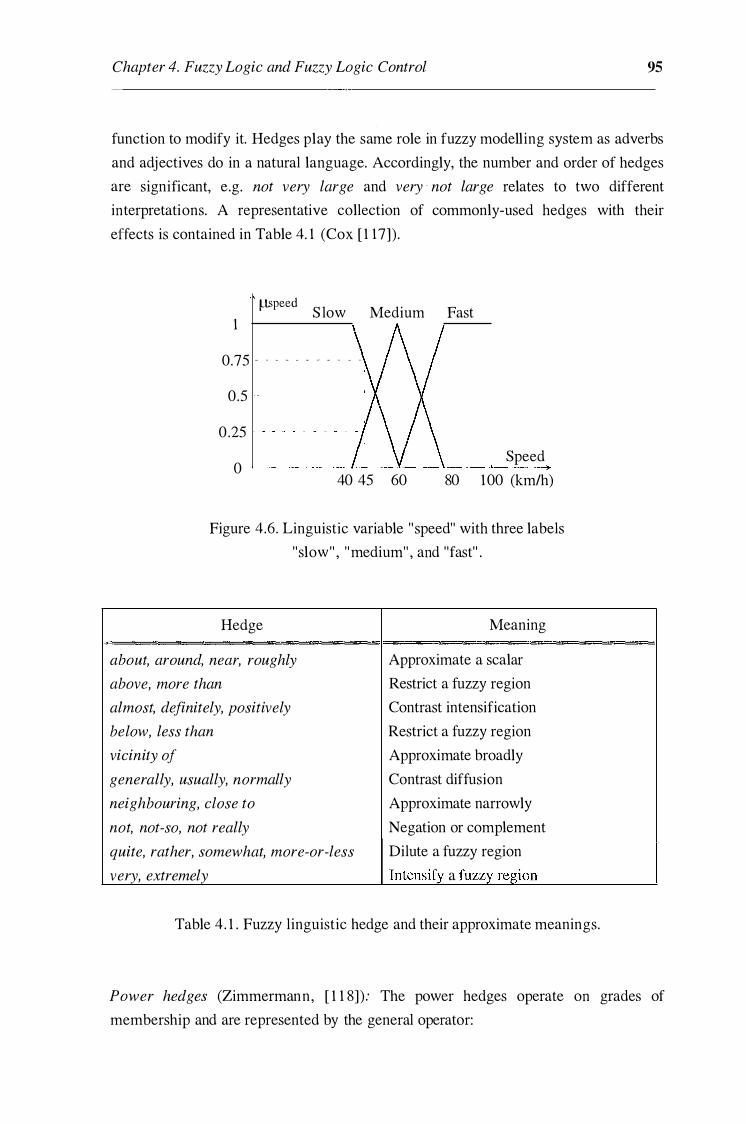
Chapter 4. Fuzzy Logic and Fuzzy Logic Control 95 function to modify it. Hedges play the same role in fuzzy modelling system as adverbs
and adjectives do in a natural language. Accordingly, the number and order of hedges
are significant, e.g. not very large and very · not large relates to two different
interpretations. A representative collection of commonly-used hedges with their
effects is contained in Table 4. 1 (Cox [ 1 17]) .
�peed S low Medium Fast
1
0.75 - - - - - - - - - - -
0 .5
0 .25
Speed 0 , ______ __,_ __ ._.. __ _,_ __ _.___._
40 45 60 80 100 (km/h)
Figure 4.6. Linguistic variable " speed" with three labels
"slow" , "medium" , and "fast" .
Hedge Meaning
about, around, near, roughly Approximate a scalar
above, more than Restrict a fuzzy region
almost, definitely, positively Contrast intensification
below, less than Restrict a fuzzy region
vicinity of Approximate broadly
generally, usually, normally Contrast diffusion
neighbouring, close to Approximate narrowly
not, not-so, not really Negation or complement
quite, rather, somewhat� more-or-less Dilute a fuzzy region
very, extremely Intensify a fuzzy region
Table 4. 1 . Fuzzy linguistic hedge and their approximate meanings.
Power hedges (Zimmermann, [ 1 1 8]): The power hedges operate on grades of
membership and are represented by the general operator:

Chapter 4. Fuzzy Logic and Fuzzy Logic Control 96
(4. 1 6)
where p is a parameter specific to a certain linguistic modifier. The exponent p used
in the hedge membership function is quite arbitrary, it can be changed depending on
our interpretation of the hedge. If p = 1 , fuzzy set is not modified. Two cases are
distinguished:
1 ) Concentration: p > 1 , fuzzy set is concentrated. Because membership functions are
assumed to be normalised, the operation of concentration leads to a membership
function that lies within the membership function of the original fuzzy set; both have
the same support, and the same membership values where the value of the original
membership function equals unity or zero.
The modifier very corresponds to p = 2 . For example, if slow speed is a fuzzy set
with membership function f.ls (x) , then very slow speed and very very slow speed are
fuzzy sets with membership function [f.ls (x)]2 , [f.ls (x)]4 , respectively. An artificial
hedge providing milder degree of concentration is the plus, whose membership function is f.lplus(U) (x) == [f.1u (x)t25 .
2) Dilation: p < 1 , fuzzy set is dilated. The operation of dilation leads to a
membership function that lies outside of the membership function of the original
fuzzy set; both have the same support, and the same membership values where the
value of the original membership function equals unity or zero.
The modifier more or less corresponds to p = 1/2 . For example, more or less slow
.speed is a fuzzy set with membership function [f.l s ( x) ] lf2 . Another hedge quite useful
is the minus, whose membership function is f.lmtnus(U) (x) = [f.lu (x)]0·75 .
4.3 Fuzzy logic and fuzzy reasoning
Fuzzy logic is a logical system that is much closer in spirit to human thinking and
natural language than traditional logic systems. As a calculus of compatibili ty , fuzzy
logic is quite different from probability which is based on frequency distributions in a
random population. Fuzzy logic describes the characteristic properties of continuously
varying values by associating partitions of these values with a semantic label (Cox
[ 1 1 7] ) . Fuzziness is different from probability. The laws of contradiction and

Chapter 4. Fuzzy Logic and Fuzzy Logic Control 97 excluded middle are broken in fuzzy logic but are not broken in probability.
Conditional probability, which must be defined in probability theory, can be derived
from first principles using fuzzy logic (Kosko [ 1 1 9]) . Much of the description power
of fuzzy logic comes from the fact that these semantic partitions can overlap (see
Figure 4.6) corresponding to the transition from one term to the next.
Fuzzy set theory serves as the basis for fuzzy logic. Fuzzy set theory stmts with some
basic concepts coming from crisp set theory, fuzzy logic also begins by borrowing
some crisp logic notions. In crisp logic, a proposition is an ordinary statement
involving terms already defined, and must be meaningful to call it "true" or "false" . A
tautology is a proposition formed by combining other propositions p, q, r, . . . , which
is true regardless of the truth or falsehood of p, q, r, . . . .
Let us start with the basic primitives of fuzzy logic: fuzzy propositions. A fuzzy
proposition represents a statement like "speed (u ) is SLOW", where SLOW is a
linguistic label , defined by a fuzzy set on the universe of discourse of speed. Fuzzy
propositions connect variables with linguistic labels defined for those variables. As in
classical logic, fuzzy propositions can be combined by using logical connectives and
and or, which are implemented by t - norms and t -conorms, respectively.
Fuzzy logic provides a means of modelling human decision making within the
conceptual framework of fuzzy logic and approximate reasoning (or fuzzy reasoning) .
In fact, reasoning with fuzzy logic is based on fuzzy rules which are expressed as
logical implications, i .e . in the forms of IF-THEN statements . In fuzzy logic, the
definition of a fuzzy implication may be expressed as a fuzzy implication function.
Various implication functions can be classified into three main categories: fuzzy
conjunction, fuzzy di.'):junction, and fuzzy implication. A fuzzy rule "IF u is A , THEN
v is B" , is represented by a fuzzy implication and is denoted by A -t B, where A and
B are fuzzy sets in the universes U and V with membership functions fl 11 and fl 8 , respectively. Membership function of the fuzzy implication, denoted by flA--7B (x, y) , measures the degree of truth of the implication between x E U and y E V.
Fuzzy conjunction: The fuzzy conjunction i s defined for all x E U and y E V by
A -t B = A*B, ( 4 . 17)
where * is an operator representing a t - norm.
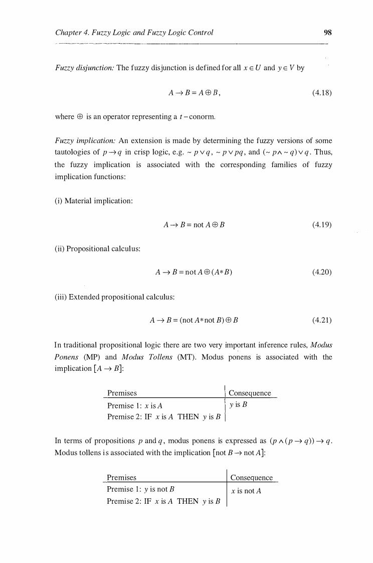
Chapter 4. Fuzzy Logic and Fuzzy Logic Control 98 Fuzzy disjunction: The fuzzy disjunction is defined for all x E U and y E V by
A -7 B = A EB B , (4. 1 8)
where EB is an operator representing a t - conorm.
Fuzzy implication: An extension is made by determining the fuzzy versions of some
tautologies of p ---7 q in crisp logic, e.g. � p v q , � p v pq , and (� pi\ � q) v q . Thus,
the fuzzy implication is associated with the corresponding families of fuzzy
implication functions :
(i) Material implication:
A ---7 B = not A EB B (4. 1 9)
(ii) Propositional calculus:
A ---7 B = not A EB (A* B) (4.20)
(iii) Extended propositional calculus:
A ---7 B = (not A* not B) EB B (4.21)
In traditional propositional logic there are two very important inference rules, Modus
Ponens (MP) and Modus Tollens (MT) . Modus ponens is associated with the
implication [A ---7 B] :
Premises Conse uence
Premise 1 : x is A y is B
Premise 2 : IF x is A THEN y is B
In terms of propositions p and q , modus ponens is expressed as (p 1\ (p ---7 q)) ---7 q .
Modus toll ens i s associated with the implication [not B ---7 not A] :
Premises Conse uence
Premise 1 : y is not B x is not A Premise 2 : IF x is A THEN y is B

Chapter 4. Fuzzy Logic and Fuzzy Logic Control 99
In terms of propositions p and q , modus tollens is expressed as ( � q 1\ (p � q))
�� p . In fuzzy logic, modus ponens is extended to Generalised Modus Ponens
(GMP) :
Premises Conse uence
Premise 1 : x is A * y is B *
Premise 2: IF x is A THEN y is B
and modus tollens to Generalised Modus Tollens (GMT):
Premises Conse uence
Premise 1 : y is B * x is A *
Premise 2: IF x is A THEN y is B
where A, A*, B, B * are fuzzy sets introduced via linguistic variables x , y (Dubois
and Prade [ 120]) . Two more families of fuzzy implication function obtained from
GMP and GMT are:
(iv) Generalisation of modus ponens:
A � B = sup{c E [0, 1 ] , A* c :=:: B} (4.22)
(v) Generalisation of modus tollens :
A � B = inf{t E [0, 1 ], B EB t :::; A} (4.23)
Based on the definitions (4. 17-4.23), many membership functions for fuzzy
implication may be generated by employing appropriate triangular norms and
conorms. For example , llA-+B (x, y) can be found from (4. 1 9) as
llA-+B (x, y) = max[l - llA (x), !l13 (y)] , (4.24a)
(4.24b)
or
ll A-7B (X, y) = 1 - !l A (x)(l - !l 13 (y)) , (4.24c)

Chapter 4. Fuzzy Logic and Fuzzy Logic Control 100
with appropriate operators for the t -norm * and t -conorm EB . From the fuzzy
conjunction ( 4. 17), membership functions for minimum implication, proposed by
Mamdani [ 109] :
(4.25)
and product implication, introduced by Larsen [ 121 ] :
(4.26)
can be obtained using minimum and algebraic product, respectively. It can be shown
that membership functions ( 4.24a-c) agree with the accepted propositional logic
definition of implication, demonstrated in Table 4.2, while neither Mamdani
membership function ( 4.25) nor Larsen one ( 4.26) does. As shown in Table 4.2,
minimum and product inferences preserve cause and effect, i .e . these implications are
fired only when the antecedent and the consequent are both true.
!lp (x) !lq (x) llp-tq (x, y) min[!lA (x), !l8 (y)] llA (X)!ls (Y)
1 1 1 1 1
1 0 1 0 0
0 1 0 0 0
0 0 1 0 0
Table 4.2. Implication with propositional logic, and min and product inference.
This is why minimum and product inferences are the most widely used inferences in
engineering applications of fuzzy logic, and referred to as engineering implications (Mendel [ 1 14]) .
A comprehensive comparison between the available fuzzy implication rules is given
in Lee [ 1 10] , based on some intuitive criteria for choosing a fuzzy implication that is
as close as possible to the input truth value function value. Although the minimum
operation rule ( 4 .25) and the product operation rule ( 4.26) of fuzzy implication do not
have a well-defined logical structure, it is shown [ 1 1 0] that they are well suited for
approximate reasoning, especially for the generalised modus ponens. The GMP,

Chapter 4. Fuzzy Logic and Fuzzy Logic Control 101 reducing to modus ponens when A* = A, B* = B, is closely related to the forward
data-driven inference, particularly useful in control systems. The GMT, reducing to
modus tollens when A* = not A, B* = not B, is closely related to the backward goal
driven inference, commonly used in expert systems.
Figure 4.7 illustratively interprets that GMP is a fuzzy composition where the first
fuzzy relation is merely a fuzzy set, A* (see Figure 4.5). Consequently, !ls* (y) can be
obtained from the sup-star composition ( 4 . 14 ) :
(4.26)
where max-min or max-product formula can be stated for modus ponens. Note that in
crisp logic, a rule is fired only if the first premise is exactly the same as the antecedent
of the rule, and the result of such rule-firing is the rule's actual consequent. On the
other hand, a fuzzy rule is fired so long as there is a non zero degree of similarity
between the first premise and the antecedent of the rule, and, the result of such rule
firing is a consequent that has a non zero degree of similarity to the rule's consequent.
u is A *
I I v is B *
----->�• IF x is A 'IHEN y is B f-------;> !-LB*(y) J.lA�s(x,y)
Figure 4.7. Sup-star composition when V = U .
4.4 Fuzzy logic control
During the past several years, fuzzy logic control, first appeared in Chang and Zadeh's
1 972 paper [ 1 3] , has emerged as one of the most active and impressive areas for
research in the applications of fuzzy set theory. Using fuzzy logic as an effective
means of capturing approximate, inexact nature of the real world, a fuzzy logic
controller provides an algorithm which can convert the linguistic control strategy
based on expert knowledge into an automatic control strategy. In particular, the
methodology of fuzzy logic control has been proven through recent successful
applications (Schwartz et al. [ 14]) to be superior to conventional control when the
processes are too complex, or when the available sources of information are

Chapter 4. Fuzzy Logic and Fuzzy Logic Control 102 interpreted imprecisely, or uncertainly. In this sense, fuzzy logic control may be
viewed as a rapprochement between conventional control and human-like decision
making techniques for improving robustness of control systems. This section gives a
brief summary of the prolific literature on fuzzy logic control and illustrates the
design procedure of a fuzzy logic controller for an overhead crane model.
4.4. 1 Fuzzy logic controllers
Fuzzy inference is the actual process of mapping from a given input to an output using
fuzzy logic. tf[ fuzzy logic controller (FLC) is a fuzzy inference system which maps an
input data vector into a scalar control output. Figure 4.8 depicts a fuzzy control
system, where the elements of the fuzzy logic controller are rules, fuzzifier, inference
engine, and defuzzifier.
, FLC I RULES I ·� FUZZIFIER DEFUZZIFIER
-
- - - -
L-1 INFERENCE
- � - - - - - - - -
1------ - - - - - - - -
l v u
PLANT
Figure 4 .8 . Block diagram of a fuzzy logic control system.
c
Once the fuzzy rules have been chosen, an FLC can be considered as a nonlinear
mapping from inputs (error e , change of error Lle ) to outputs (control signal u ) . This
mapping can be expressed quantitatively as u = f(e, Lle) . The design of an FLC is
how to obtain explicitly this relation so that the control requirements are satisfied.
Rules may be provided by experts or can be extracted from numerical data. In either
cases, engineering heuristic rules are expressed as a collection of IF-THEN
statements . Each rule consists of linguistic variables, linguistic terms, logical
connections, and implications . Each linguistic term is a fuzzy set associated with its
fuzzy membership function.
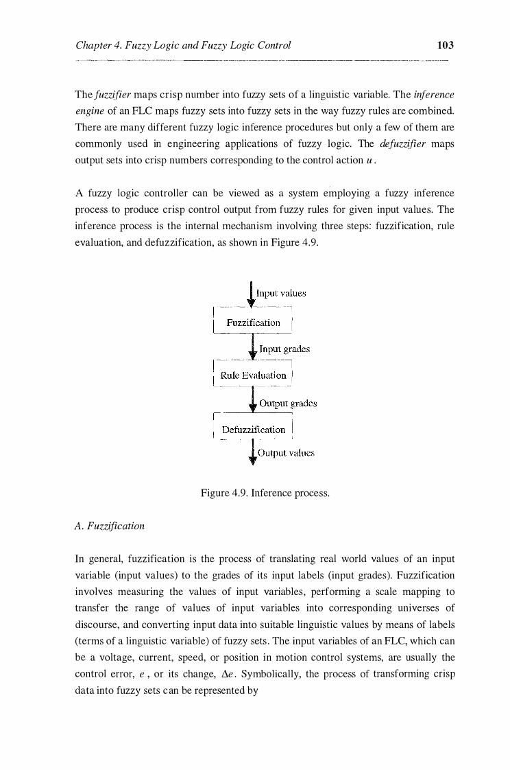
Chapter 4. Fuzzy Logic and Fuzzy Logic Control 103 The fuzz�fier maps crisp number into fuzzy sets of a linguistic variable. The inference engine of an FLC maps fuzzy sets into fuzzy sets in the way fuzzy rules are combined.
There are many different fuzzy logic inference procedures but only a few of them are
commonly used in engineering applications of fuzzy logic. The defuzzifier maps
output sets into crisp numbers corresponding to the control action u .
A fuzzy logic controller can be viewed as a system employing a fuzzy inference
process to produce crisp control output from fuzzy rules for given input values. The
inference process is the internal mechanism involving three steps: fuzzification, rule
evaluation, and defuzzification, as shown in Figure 4.9.
Figure 4.9. Inference process.
A. Fuzzification
In general, fuzzification is the process of translating real world values of an input
variable (input values) to the grades of its input labels (input grades). Fuzzification
involves measuring the values of input variables , performing a scale mapping to
transfer the range of values of input variables into corresponding universes of
discourse, and converting input data into suitable linguistic values by means of labels
(terms of a linguistic variable) of fuzzy sets . The input variables of an FLC, which can
be a voltage, current, speed, or position in motion control systems, are usually the
control error, e , or its change, �e . Symbolically, the process of transforming crisp
data into fuzzy sets can be represented by

Chapter 4. Fuzzy Logic and Fuzzy Logic Control 104 x = fuzzifier(x0 ) , (4.27)
where x0 is a crisp input value ( e or 11e ) , x is a fuzzy set, and fuzzifier is a
fuzzification operator . In order to develop useful rules, appropriate membership
functions associated w ith each label should be well chosen. Therefore, it is necessary
to have a good intuitive feel for the nature of the variables. The defining membership
functions for all variables would be based on designer's intuitive assumptions, just as
the rules themselves are. The fuzzification process also provides necessary conditions
for defining linguistic control rules and fuzzy data manipulation in an FLC, including
the discretisation/normalisation of the universes of discourse, fuzzy partition of the
input and output spaces, and choice of the appropriate membership function of a
primary fuzzy set.
Discretisation of a universe of discourse is the process of quantising it into a certain
number of segments (quantisation levels) with corresponding labels and thus, forming
a discrete universe. A fuzzy set is then defined by assigning grade of membership
values to each label . A scale mapping is needed to transform measured variables into
values in the discretised universe. The choice of quantisation levels determines how
fine a control can be obtained. Normalisation of a universe requires discretising it into
a finite number of segments. Each segment is mapped into a suitable segment of the
normalised universe w hich normally is the closed interval [0, 1 ] or [ -1 , 1 ] .
In general, a linguistic variable is associated with a term set. Each term in the term set
is defined on the same universe of discourse. A fuzzy partition, then, determines the
number of terms in a term set. This number affects the granularity of the fuzzy
control. Figure 4. 10 shows a fuzzy partition in the normalised universe [ -1, 1] with
seven terms: NB, NM, NS , ZE, PS, PM, and PB , which mean negative big, negative
medium, negative small, zero, positive small, positive medium, and positive big,
respectively.
- 1 0 0.25 1
Figure 4. 1 0. A fuzzy partition representation.

Chapter 4. Fuzzy Logic and Fuzzy Logic Control 105
A membership function (MF), which defines how each point in the input space of a
label is mapped to a degree of membership between 0 and 1 , can principally take any
nonlinear or piece-wise linear form. The latter is either a triangular or trapezoidal
functions as shown, for example, in Figures 4.6 and 4. 10. They are the simplest and
most commonly-used in engineering applications. The vertex of a triangular fuzzy
label usually corresponds to the mean value of a data set, while the base is twice the
standard deviation of the data set.
Crisp value can be converted into a fuzzy singleton (see Figure 4.2) within a certain
universe of discourse. This kind of membership function is widely used in fuzzy
control applications because it is natural and easy to implement. The other commonly
used membership functions, with universes of discourse scaled to [0, 1 ] , are described
below. The Gaussian MF, determined by
( (x - c)2 )
fl(x, cr, c) = exp -2cr
2 , (4.28)
where a and c are two positive parameters, has the forms of Figure 4. 1 l (a). A combination of two Gaussian membership functions gives the two-sided form of
Figure 4. 1 1 (b).
0.8
0.6
0.4
0.2 """'�' 0 0
--o----;r· '· / \ I \ I \ I \
I \
/ \ I \
I \ I \
I \ / \\
/./ \....,
0.2 0 .4 0.6 0.8
(a)
................. , ....... ..... .
0.8
0.6
0.4
0.2
·-...... ___ 0 / 0 0.2 0.4 0 .6
(b)
Figure 4. 1 1 . Gaussian membership functions :
0.8
(a) cr = 0. 15, c = 0. 5 , and (b) cr1 = 0. 1, c1 = 0. 3, cr2 = 0. 2, c2 = 0. 5 .

Chapter 4. Fuzzy Logic and Fuzzy Logic Control 106 The generalised bell-shape MF with the form of Figure 4. 12 is described by
!l(x, a, b, c) =
I 12h ' 1 + x - c
a
1 (4.29)
where a > 0, b > 0, and c > 0 . Both Gaussian and bell-shape membership functions
have the advantage of being smooth and nonzero at all points, however they cannot
specify asymmetry. Open (left or right) forms can be synthetised using exponential
membership functions . Figure 4. 1 3 shows an open right MF
where cr > 0 .
I
I 0.8 I i
0.6 / I
0.4 J 0.2 I / / / , .. _.. .. _.,..., .. 0 ---
0 0.2 0.4 0.6
X !l(x, cr) = 1 - exp( --) , (j
0.8
0.6
0.4
0.2
0.8 0.2
(4.30)
0.4 0 .6 0 .8
Fig. 4 . 1 2. Bell MF, a = 0. 2 , b = 2, c = 0. 6 . Fig. 4. 13 . Exponential MF, cr = 0. 2 .
The sigmoid can also b e used to specify asymmetric membership functions, which are
important in certain applications. Figure 4. 14( a) plots the form of an open right
sigmoidal MF defined by
2 !l(X, a, c) = , 1 + exp( -a(x - c))
(4.30)
where a > 0 and c > 0 . An asymmetric and closed (i.e. not open to the left or right) M
can be synthetised by the difference of two sigmoidal functions as represented in
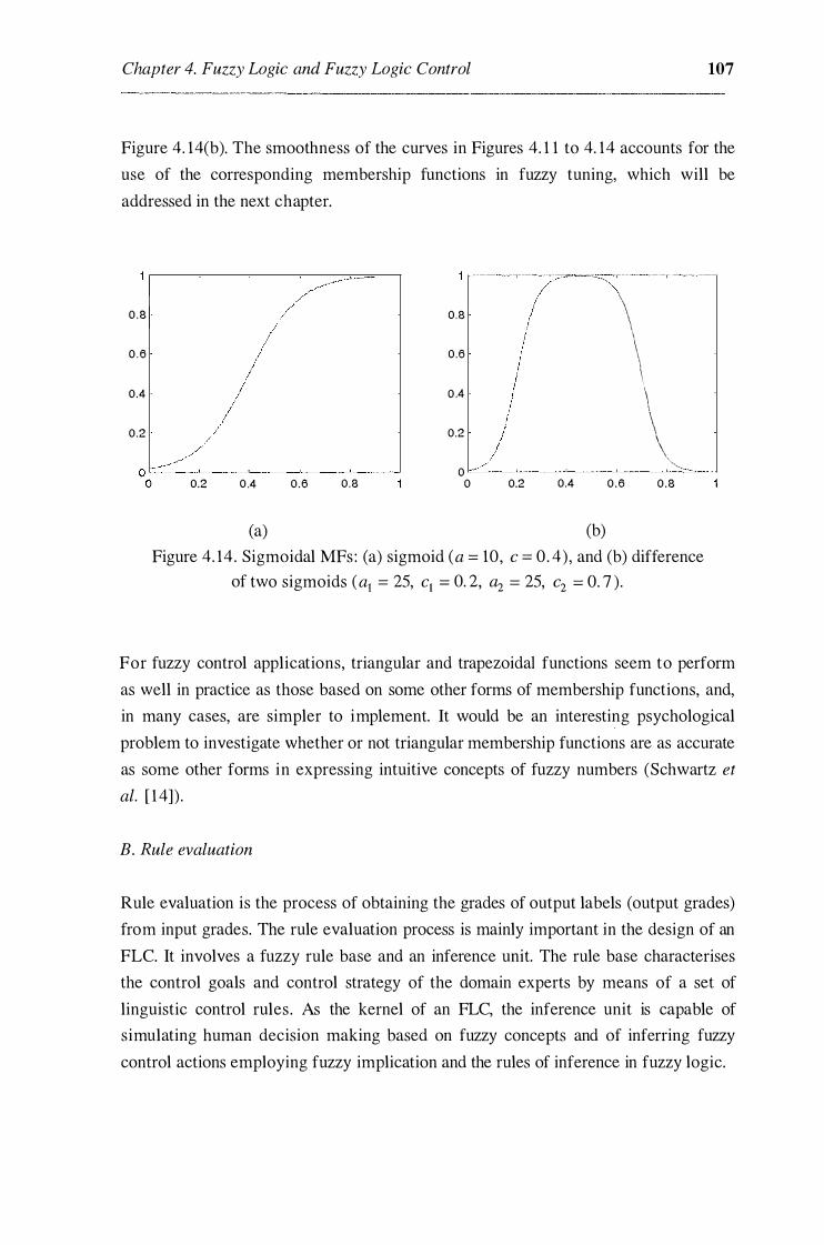
Chapter 4. Fuzzy Logic and Fuzzy Logic Control 107 Figure 4. 14(b). The smoothness of the curves in Figures 4. 1 1 to 4. 14 accounts for the
use of the corresponding membership functions in fuzzy tuning, which will be
addressed in the next chapter.
0 .8
0 .6
0.4
0.2
.. "\ \ \ 0.8 \
\ 0 .6 \ \ 0 .4 \
\ \ 0.2 \ \
0 "···.
0.2 0 .4 0.6 0 .8 0 0.2 0.4 0 .6 0 .8
(a) (b)
Figure 4. 14. Sigmoidal MFs: (a) sigmoid (a = 10, c = 0. 4) , and (b) difference
of two sigmoids ( a1 = 25, c1 = 0. 2, a2 = 25, c2 = 0. 7 ) .
For fuzzy control applications, triangular and trapezoidal functions seem to perform
as well in practice as those based on some other forms of membership functions, and,
in many cases, are simpler to implement. It would be an interesting psychological
problem to investigate whether or not triangular membership functions are as accurate
as some other forms in expressing intuitive concepts of fuzzy numbers (Schwartz et al. [ 14]) .
B. Rule evaluation
Rule evaluation is the process of obtaining the grades of output labels (output grades)
from input grades. The rule evaluation process is mainly important in the design of an
FLC. It involves a fuzzy rule base and an inference unit. The rule base characterises
the control goals and control strategy of the domain experts by means of a set of
linguistic control rules . As the kernel of an FLC, the inference unit is capable of
simulating human decision making based on fuzzy concepts and of inferring fuzzy
control actions employing fuzzy implication and the rules of inference in fuzzy logic.

Chapter 4. Fuzzy Logic and Fuzzy Logic Control 108 Based on expert knowledge and fuzzy reasoning, the rule base of an FLC can be
formatted infuzzy conditional statements as follows:
Ri : IF (set of conditions) THEN (set of consequences), (i = 1 , 2, . . , n ) (4. 3 1 )
where the antecedents and the consequents of these rules are associated with linguistic
values (labels). A fuzzy control rule is a fuzzy conditional statement in which the
antecedent is a condition determined in an application domain and the consequent is a
control action for the p lant. A rule base is normally formed by a set of fuzzy control
rules combined by using the sentence connectives and and also. In most FLCs, the
sentence connective and is usually implemented as a fuzzy conjunction in a Cartesian
product space, in which the underlying variables take values in different universes of
discourse. When the ordering of the fuzzy rules are immaterial, the sentence
connective also is used with the associated properties of commutativity and
associativity. From a practical point of view, the union operator is normally used for
the connective also for constructing fuzzy models (Lee [110]) . The overall system
behaviour can then be characterised by a single fuzzy relation R which is the combination of the fuzzy relations Ri . Symbolically,
(4.32)
where also represents a sentence connective.
In general, there are four modes of deriving fuzzy control rules: from expert
experience and control engineering knowledge, from human operator's control
actions, from the fuzzy model of a process, and from learning. A fuzzy control rule
normally has the form of a fuzzy conditional statement relating the state variables in
the antecedent and the control action in the consequent. Most FLCs employ
engineering knowledge and experience which are expressed in the language of fuzzy
IF-THEN rules based on an introspective verbalisation of human expertise or an
interrogation of experienced experts or operators. Many industrial control systems can
be empirically controlled by skilled human operators without any quantitative models
in mind. As pointed out by Sugeno [ 123] in order to automate such processes, it is
expedient to express the operator's control rules as fuzzy IF-THEN rules using
linguistic variables. Fuzzy control rules can also be generated based on the linguistic
description of the dynamic characteristics of the plant known as fuzzy model .
Although this approach is somewhat more complicated, it yields better performance

Chapter 4. Fuzzy Logic and Fuzzy Logic Control 109 and reliability, and provides a more attractable structure for dealing theoretical with
the FLC (see, e.g. , Cao et al. [ 124]) . Focusing on the ability to create fuzzy control
rules and to modify them based on experience (learning), Procyk & Mamdani [ 1 25]
described the first self-organising controller with a hierarchical structure of two rule
bases : the general rule base and the "meta-rules" . The latter exhibit human-like
learning ability to create and modify the general rule base according to the desired
overall performance of the system. Self-organising control (Shao [ 126]) or fuzzy
learning systems with model reference (Kwong et al. [ 127]) and neuro-fuzzy approach
(Jang & Sun [ 128]) have become increasingly interesting subjects for fuzzy control
studies.
In a typical fuzzy system, the FLC rule base describes the relationship between the
change of the control !1u(k) = u(k) - u(k - 1) on one hand, and the error e(k) and its
change !1e(k) = e(k) - e(k - 1) on the other hand, where k is discretised time. The
actual controller output u(k) , first proposed by Mamdani & Assilian [ 129] ,
u(k) = u(k - 1) + 11u(k) , (4.33)
is called the Mamdani-type FLC. The similarity between the Mamdani-type FLC and
the conventional propotional-integral (PI) controller is that the change of the control
!1u(k) is calculated depending on the error e(k) and its change !1e(k) :
!1u(k) = f(e(k) + 11e(k)) = Kp11e(k) + K1e(k) , (4.44)
where Kp and K1 are the parameters of the proportional-integral (PI) controller. If the
output variable is not the change of the control action 11u(k) , but the control value
u(k) itself, we obtain a control law
u(k) = f(e(k), 11e(k)) , (4.45)
which is similar to the known proportional-derivative (PD) control law. An example
of a PD-like FLC rule base is presented as follows:
IF the error e(k) is Positive AND the change of error 11e(k) is Positive THEN
the control u(k) is Positive, IF the error e(k) is Positive AND the change of error !1e(k) is Approximately
zero THEN the control u(k) is Positive,

Chapter 4. Fuzzy Logic and Fuzzy Logic Control
IF the error e(k) i s Positive AND the change of error l:!.e(k) is Negative THEN the control u(k) is Approximately zero,
IF the error e(k) is Approximately zero AND the change of error l:!.e(k) 1s
Approximately zero THEN the control u(k) is Approximately zero, IF the error e(k) is Approximately zero AND the change of error l:!.e(k) 1s
Positive THEN the control u(k) is Positive, IF the error e(k) is Approximately zero AND the change of error l:!.e(k) is
Negative THEN the control u(k) is Negative. IF the error e(k) is Negative AND the change of error t:.e(k) is Positive
THEN the control u(k) is Approximately zero, IF the error e(k) is Negative AND the change of error t:.e(k) is Approximately
zero THEN the control u(k) is Negative, IF the error e(k) is Negative AND the change of error t:.e(k) is Negative
THEN the control u(k) is Negative,
110
The fuzzy control rules may be formulated into a look-up table as shown in Table 4 .3 ,
where the linguistic l abels N, Z, and P mean negative, positive, and approximately
zero. The look-up table can be a significant tool for simplification of the internal
representation of an FLC.
e(k) N z p t:.e(k)
N N N z z N z p p z p p
Table 4.3 . Fuzzy rules for the control action u(k) of a PD-like FLC.
The PD-like FLC can be extended by including in (4.45) the sum of the errors k-1
I_e(k) = Le(l) with the fuzzy mapping : 1=0
u(k) = f(e(k), I. e(k), l:.e(k)) , ( 4.46)
Chapter 4. Fuzzy Logic and Fuzzy Logic Control 111 which i s similar to the proportional-integral-derivative (PID) control algorithm. The
difference between conventional controllers and FLCs is that the fuzzy control
relationship is nonlinear, in general . Naturally, it is rather unrealistic to expect that an
operator or expert can determine reasonable control rules , considering higher
differences of the control error. This is why the most common FLCs are the PI-like or
PD-like controllers (Yager & Filev [ 1 30]) .
Completeness of an FLC i s its capability of inferring a proper control action for every
state of process (Lee [ 1 10]) . The union of the supports on which primary fuzzy sets
are defined should cover the related universe of discourse of a fuzzy partition in
relation to some level set £ . This property is called c. -completeness. Usually, the
level £ is chosen at the crosspoints as shown in Figure 4. 10 so that it always exists a
dominant rule associated with the grade of membership greater than 0.5 at any scaled
input value (e.g. at 0.25 in Figure 4. 1 0, the rule associated with the label PS will be
dominant) . Completeness can also be incorporated into fuzzy control rules depending
on design experience and engineering knowledge. An additional rule can be added
whenever a fuzzy condition is not included in the rule base to show that no control
action will result. Or whenever the degree of partial match between some inputs and
the predefined fuzzy conditions is lower than some level £ , the additional rule then
indicates that no dominant rule will be fired.
C. Defuzzification
The defuzzification process is the final stage in a fuzzy reasoning system involving
the selection of a representative element based on the output fuzzy subset.
Defuzzification is a mapping from a space of fuzzy control actions defined over an
output universe of discourse into a space of real world (crisp) control actions. A
defuzzification strategy is aimed at producing a non-fuzzy control action that
represents the possibility distribution of an inferred fuzzy control action. Many
strategies have been proposed in the literature; however their scientific bases are so
inadequate that defuzzification is considered as an art rather than a science (Mendel
[ 1 1 4] ) . For the purpose of computational simplicity, the maximum criterion, mean of
maxima and the centre of area used as defuzzification methods.
The maximum criterion method examines the fuzzy set B and selects as its output the
value y * the possibility distribution, obtained by an aggregation operator using fuzzy
reasoning, J.1 B (y) , is a maximum. Figure 4. 1 5 depicts two undesirable cases of this

Chapter 4. Fuzzy Logic and Fuzzy Logic Control 112 defuzzification strategy. The first case can lead to a hang-up because the maximum of
llB (y) occurs for a range of y (Figure 4. 1 5(a)) . Peculiar values can be resulted when
using maximum defuzzifier (Figure 4. 15(b)) .
J.lB(y) B l · B2 ·,
0 ---'---�---�...--�
y y* Y2 y 0
(a)
J.lB(y) B L ' , B2 . :
� ' '
' ' ' '
� � y*=y2 y
(b)
Figure 4 . 1 5 . Undesirable cases of defuzzification with the maximum method.
The Mean of Maxima method (MOM) determines a control action which represents
the mean value of all local control actions having maximal membership grades. More
specifically, in the case of a discrete universe, the MOM strategy gives:
(4.47)
where y j is the support value at which the membership function reaches the
maximum value J.l B (y j ) , and q is the number of such support values. If the maximum
value of the possibility distribution 11 B (y) occurs at a single point, the MOM
defuzzifier reduces to the maximum defuzzifier and the crisp value obtained by the
MOM strategy in some cases does not make sense as illustrated in Figure 4. 1 6.
J.!B(Y)
0 y l y* y2 y
Figure 4. 1 6 . Case showing the MOM defuzzification makes no sense.
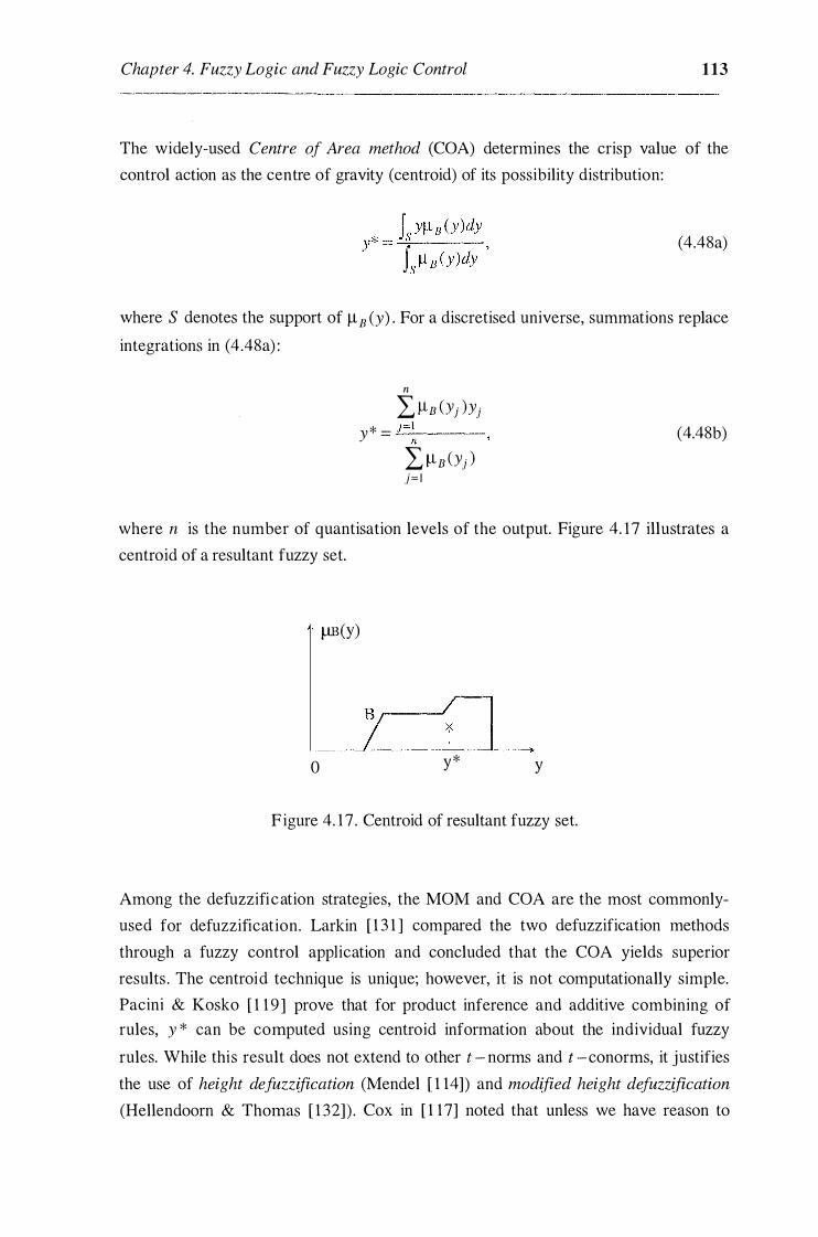
Chapter 4. Fuzzy Logic and Fuzzy Logic Control 113 The widely-used Centre of Area method (COA) determines the crisp value of the
control action as the centre of gravity (centroid) of its possibility distribution:
(4.48a)
where S denotes the support of 1113 (y) . For a discretised universe, summations replace
integrations in (4.48a) :
n LYB (Yj )Yj
y* = .::....j =-�----LilB (Yj ) }= I
(4.48b)
where n is the number of quantisation levels of the output. Figure 4. 17 illustrates a
centroid of a resultant fuzzy set.
J..lB(Y)
0 y* y
Figure 4. 17 . Centroid of resultant fuzzy set.
Among the defuzzification strategies, the MOM and COA are the most commonly
used for defuzzification. Larkin [ 1 3 1 ] compared the two defuzzification methods
through a fuzzy control application and concluded that the COA yields superior
results . The centroid technique is unique; however, it is not computationally simple.
Pacini & Kosko [ 1 1 9 ] prove that for product inference and additive combining of
rules, y * can be computed using centroid information about the individual fuzzy
rules. While this result does not extend to other t - norms and t -conorms, it justifies
the use of height defuzzification (Mendel [ 1 14]) and modified height defuzzification
(Hellendoorn & Thomas [ 1 32]) . Cox in [ 1 17] noted that unless we have reason to

Chapter 4. Fuzzy Logic and Fuzzy Logic Control 114 suspect that our model will behave better under other defuzzification techniques, the
centroid method appears to provide a consistent and well-balanced approach.
Although by nature, the centroid method is sensitive to the height and width of the
total fuzzy region, it i s well suited to handling solution regions that are maintained as
sparse singletons. The method using singletons (single vertical points) instead of
fuzzy set membership functions to describe output labels is referred to as Sugeno-style
fuzzy inference method while the inference method discussed thus far using fuzzy sets
to describe the output labels is called Mamdani's method. In Sugeno's method, the
aggregation step is no longer necessary and the COA defuzzification method is
slightly simplified. The centroid is calculated without a numerical integration of the
entire fuzzy set surface as in ( 4 .48a) . Instead, the domain value at each singleton is
multiplied by the height (truth membership value) of the singleton. This technique, in
general, provides an equivalent centroid as to the centroid found by taking the area
across an entire fuzzy set. Because it is more compact and computationally efficient
representation than the Mamdani system, the Sugeno-style inference method lends
itself to adaptive techniques (Jang & Gulley [ 1 33]).
4.4.2. An example of fuzzy logic control
Over the last five or ten years, fuzzy models have supplanted more conventional
technologies in many scientific applications and engineering systems, especially in
control systems and pattern recognition. This wide and diverse range of successful
applications of fuzzy technology is, in the main, responsible for the increasing interest
in the subject area (Schwartz et al. [ 14]) . Among new trends in control theory, fuzzy
logic issues have been introduced to electrical engineering curriculums in tertiary
institutions (Ha & Negnevitsky [ 1 6]) .
In this section, the design and implementation of a fuzzy logic controller for an
overhead crane model , reported in Negnevitsky, Ha et al. [ 1 34] is described as an
illustrative example. Here the problem is how to move a load from an initial position
to a specified final one with minimal pendulum-like swing of a load. The crane system
is subject to uncertainty in mass and chain length. Crane operations have been
successfu1ly performed in traditional installations which are totally reliant on the skill
of human operators without having any quantitative knowledge of the underlying
dynamics. The model is thus an example when fuzzy control may be applied to obtain
a controller which can demonstrate robustness against external disturbances and
parameter variations, and nonlinearity.

Chapter 4. Fuzzy Logic and Fuzzy Logic Control 115
A. Plant description
A simple two-degree-of-freedom controlled model of the overhead crane system is
used. It consists of a trolley, which can be moved along tracks carved out from the
wooden base of the model. The trolley position is controlled using a de motor,
connected to a pulley system. A pendulum in the form of a metal rod is suspended from
the centre of the trolley and imitates the cable and load of an actual crane as shown in
Figure 4. 1 8. The control goal is to move the trolley and the mass underneath from an
initial horizontal position to a final one as fast as possible while suppressing the load
swinging. This model is well known and used in many laboratories. The second
equation of Lagrange is applied to find the crane dynamics. The horizontal position of
the trolley, the velocity of the trolley, the angle of the chain, the angular velocity of the
chain, and the force exerted by the drive onto the trolley are denoted by x1 , x2 , x3 , x4
and f , respectively. The plant state equation obtained is a nonlinear one which can then
be written as :
with
(4.49)
<I> = _ g(M + m) s in x3 + (f + Lmx; sin x3 ) cos x3 and f
= K u - Kb x2 /P
L(M + m sin2 x3 ) 1 Rp '
Figure 4. 1 8 . Schematic of an overhead crane model.
Chapter 4. Fuzzy Logic and Fuzzy Logic Control 116
where g is the gravitational acceleration, M is the trolley mass, p is the trolley motor
drum radius, and Kf ' Kb and R are the motor torque constant, back emf constant and
armature resistance, respectively. The load mass m and the chain length L are the
changing parameters of the crane system. The motor voltage u is used to control both
the trolley position and the load mass. In order to demonstrate the capability of the
fuzzy control system to suppress the load swinging due to any disturbance deviations
of the swing angle, the nonlinear state equations are used to describe the crane system
dynamics instead of the linearised ones .
B. Fuzzy logic controller design
The control goal can be achieved by conventional methods (cascade control , pole
placement, optimal control, etc.) . However, a skilful operator is also perfectly capable
of accomplishing the task. The problem is how to adapt the human experience to
design the controller u sing fuzzy logic. Dealing with some uncertainty about the load
mass or the chain length, an operator should control the motor voltage coarsely to
move the trolley to a specified position and finely to reduce the load swing. In other
words, because the swing of the load is to be kept minimal throughout the motion of
the trolley, i .e. the swing should be minimal irrespective of the trolley position, the
position of the trolley and the swing of the load are controlled using two separate fuzzy
control units. The position fuzzy controller (XFC), consequently, depends on the
position error e and the past value u1 of the controller output u . Then, the output v of
the XFC and the swing angle 8 are used to adjust the controller output through the
swing fuzzy controller (SFC). Figure 4 . 1 9 shows the overall structure used for the
control of the overhead crane. These fuzzy controllers are cascaded with the output the
XFC fed into the SFC. As the swing of the load is dependent on the acceleration of the
trolley, the output of the SFC gives the change bu of the control voltage u to the
system. The control signal u to the system is obtained as by a Mamdani-type (PI-type)
fuzzy logic controller (4.33) :
u(k) = u(k - 1) + bu . (4.50)
A delay voltage u1 = u(k - 1) is used as the input to the XFC instead of the current
system control value to reduce the acceleration of the trolley and thus, to minimise the
load swing. The first step for designing a fuzzy controller is to fuzzify the controller
inputs and outputs. These variables are described by linguistic labels NB, NM, NS, ZE,
PS , PM and PB which mean negative big, negative medium, negative small, zero,

Chapter 4. Fuzzy Logic and Fuzzy Logic Control 117
positive small, positive medium and positive big, respectively. The problem is how to
choose the corresponding membership functions for each label of the inputs (position
error e , delay voltage u1 , SFC input v , and swing angle 8 ) and outputs (XFC output v
and control voltage change 8u ) .
XFC SFC SYSTEM
+
u = u(k-1)
Figure 4 . 19 . Fuzzy logic controller for the crane system.
The proposed membership functions for XFC is shown in Figure 4.20 . Triangular
membership functions are used for the input labels of position error e and delay
voltage u1 (Figure 4.20a-b ) , and singletons for the output membership functions
(Figure 4.20c ). Figure 4.2 1 shows the membership functions for SFC labels of the
swing angle 8 , the voltage input, and the control voltage change ou (SFC output) . The
fuzzy rules are written as a representation of human operations to control the trolley
and the load underneath. Following typical instructions of an operator for the control
task, a fuzzy rule can be expressed like
• "If the position error is positive big and the delay voltage is negative big then the
position controller output is positive big" , or
• "If the swing angle is positive medium and the position controller output is positive
small then the control voltage change is positive medium", etc.
A proposed set of fuzzy rules for the XFC and SFC is presented in Tables 4.4 and 4.5.
They are developed in the Fuzzy Inference Units (FlU) using the Fuzzy Inference
Development Environment (FIDE') software package (Aptronix [ 1 35]) .

Chapter 4. Fuzzy Logic and Fuzzy Logic Control 118
NB PB
-100 -50 -20 0 20 50 100
(a)
(b)
NB NM NS ZE PS PM PB
0 -5 -4 -2 -I
(c)
Figure 4.20. Membership functions for: (a) error, (b) delay voltage, (c) XFC output.

Chapter 4. Fuzzy Logic and Fuzzy Logic Control
NB
0 -5
NB PB
(a)
NM NS ZE PS PM
NB NM NS
-3.5 -2.5 -1.5
(b)
ZE
(c)
PS PM
15 2.5
119
PB
PB
3.5
Figure 4.21. Membership functions for: (a) angle, (b) voltage input (c) SFC output.

Chapter 4. Fuzzy Logic and Fuzzy Logic Control 120
XFC e NB NM NS ZE PS PM PB
ul v
NB ZE PS PM PB PB PB PB
NM NS ZE PS PM PM PM PB
NS NM NS ZE PS PS PM PB
ZE NB NM NS ZE PS PB PB
PS NB NM NS NS ZE PS PM
PM NB NM NM NM NS ZE PS
PB NB NB NB NB NM NS ZE
Table 4.4. Fuzzy rules of XFC.
SFC 8 NB NM ZE PM PB
v 8u
NB NB NB NB NM NS
NM NB NM NM NS ZE
NS NB NM NS ZE PS
ZE NM NS ZE PS PM
PS NS ZE PS PM PB
PM ZE PS PM PM PB
PB PS PM PB PB PB
Table 4.5. Fuzzy rules of SFC.
Surface views for the two control units are shown in Figure 4.22 and 4.23 . A Fuzzy
Inference System is created by the composer tool to configure the whole system, as
presented in Figure 4 .24 .
Simple arithmetic calculations in the system are performed by the Fuzzy Operation
Units (FOU). The crane dynamics is represented by the Fuzzy Execution Unit (FEU)
with the fourth order Runge-Kutta integration algorithm for the non-linear state
equations (4.49) . This unit links executable 'C' code developed outside of FIDE' to the
integrated system. Debugging options are utilised to analyse and fine-tune the final
design. The FlU files can also be translated to assembly code which is used for real
time control of the crane model.

Chapter 4. Fuzzy Logic and Fuzzy Logic Control 121
Figure 4.22. Surface view of the position fuzzy controller XFC.
Figure 4.23 . Surface view of the swing fuzzy controller SFC.
Figure 4.24. Composer/Graphics of the control system.

Chapter 4. Fuzzy Logic and Fuzzy Logic Control 122 C. Simulation and experimental results
The numerical parameters of this overhead crane model are given in the Table 4.6. The
FIDE' software package provides facilities for debugging, analysing, and fine tuning
the membership functions and fuzzy rules to improve control quality. The position and
swing responses obtained by simulation are shown in Figure 4.25 (dotted lines). A
reference position for the trolley is achieved after a settling time of about 3 seconds
with a maximal swing less than 5 degrees .
Parameter Value
Chain length, m 0.5
Trolley mass, kg 1
Load mass, kg 0.25
Motor torque constant, Nm/A 0.0066
Motor back emf constant, V/rad/s 0.0066
Motor armature resistance, ohm 0.67
Trolley motor drum radius, m 0.0 1
Gravitational acceleration, m I s2 9 .8 1
Table 4.6. Crane system parameters.
A photograph of the laboratory set-up is displayed in Figure 4.26. The crane model is
driven by a 57W DC-motor of the type UGTMEM-03MB2, supplied with a Pulse
Width Modulation (PWM) bridge. A rotary potentiometer connected to a shaft to
which the pendulum rod is connected, is used to obtain a measurement of the
pendulum swing angle. The trolley position is measured by using another rotary
potentiometer, mounted on the motor shaft. The analog readings are converted to
digital values with an ADC. The membership functions and fuzzy-rule-base for the
XFC and SFC are realised using 'C' code generated from the FIDE' package. The host
computer, a 486 PC/AT, performs on-line processing of the appropriate crisp output
control voltage. This voltage is fed to the PWM circuit for the de motor through a
DAC.
The experimental position and swing responses are as shown in Figure 4.25 (solid
lines) to compare with the simulation results (dotted lines) . The results obtained
coincide well with those obtained from simulation.

Chapter 4. Fuzzy Logic and Fuzzy Logic Control 123
700
'E 600 � �
5 500 1: 0
400 -:;:::; '(ij 0
300 0.. ;::.. � 200 0
.... 1-0
0 CX) � '<!- C\J '<!- CX) co '<!- C\J co ci C\i cr5 -i u) 0 r....:
Time (s) (a)
1 5
1 0 Ui' CIJ CIJ ... Cl
5 CIJ :!:!.. Cl c: '§: 0 (/) '0 00 <D <:t N 113 "<i I!) <ci r-..: 0
...1 -5
- 1 0
Time (s) (b)
Figure 4.25. Simulation (dotted lines) and experimental (solid lines) (a) position, and (b) swing responses.
Figure 4.26. A photograph of the model.

Chapter 4. Fuzzy Logic and Fuzzy Logic Control 124
The experimental responses with proportional (P) and proportional-integral (PI)
control lers are shown in Figure 4.27 to confirm the fuzzy logic controller advantage in
reducing load swing. The influences of external disturbances on the load swing and
variations of the load mass and chain length are investigated. Figure 4.28 depicts the
swing responses of the crane system with an initial swing angle of 36 degrees and
different load masses. The swing responses with varying pendulum length are shown
in Figure 4.29. The results obtained demonstrate the system insensitivity with respect
to any variations.
40 -30
� . . I t ��\ f' " I' I \
I ' ,· ' •• I I I •• \ I : �· 0 1 I 1 I I : I I : : I ' I : I
20 I I I \ I I
� : : �'"\ .' : � I t/ I 1 I
!!.! 1 0 : /: \ : :,{�, : : /\ : /\ . :r " 1 �\ : g' : I : \ ; _..;r � � , \ . " \ : ,': \ / • \ : :;; 0
c .-'\':'oo./ : � �\ ��� \��� � ,;,_ \'r.o. / •• --r 1.: IN: � -� -1 0 • ,\._'=] : ,... ,' V "! • 'X/ : • \/ --r, ;\o/ : tO :'-./ r--: : I (j) : 1 \ I I : I f : I : : \ -2o ;_ ,: \ ; : : \ : ; -30 • .. -40 ' ., , " '
. . . . . . . . � '
·50 �-----------�---------�--------------�
Figure 4.27 . Swing responses with FLC (solid line), P (dotted line), and
PI ( dashe5j,line) controllers. ' / ,;
-4 ········· . . Time (s)
4:s· 5.6 6.4 7.2
- 50g --- 250g . . . . . . 500g
Figure 4.28 . Swing responses with an initial angle deviation and
different masses (50, 250, 500 g).

Chapter 4. Fuzzy Logic and Fuzzy Logic Control
-�-��
4.8
__ J=400
- - - 1=200 • • • • • , 1= 1 0
Figure 4 .29. Swing responses with chain length variations
( 1 00, 200, 400 mm).
'
125
In the example described above as in many of its applications, an FLC is either
designed by a domain expert or in close collaboration with domain experts .
Knowledge acquisition in FLC applications plays an important role in determining the
control performance. However, domain experts and skilled operators do not structure
their decision making by any formal way. Although fuzzy logic provides an effective
tool for linguistic knowledge representation and Zadeh's compositional rule of
inference serves as a useful guideline, more efficient and more systematic methods for
knowledge acquisition are still needed as discussed in the next section.
4.5 Fuzzy control: pros, cons, and perspective
Classical control theory has been well-developed and provides an effective toll for
mathematical system analysis and design when a precise model of a system is
available. In a complementary way, fuzzy controllers have found many of practical
applications as a means of replacing a skilled operators. Fuzzy control has emerged as
a practical alternative to several conventional control schemes and, in general, can be
applied in a broad class of systems where successful applications have been shown
(Schwartz et al. [ 14]) . Moreover, their superiority is found in many nontraditionally
modelled industrial processes such as linguistically controlled devices and systems
with unmodelled effects and uncertainties that cannot be precisely described by
mathematical formulations. While fuzzy logic control is attractive for dealing with
uncertainty, non-linearity, and complexity in systems, it is lacking in documented
theory to direct the design process and is reliant on common sense engineering

Chapter 4. Fuzzy Logic and Fuzzy Logic Control 126
heuristics. Indeed, the design of fuzzy controllers is usually performed in an ad hoc
manner where it is often difficult to choose the controller parameters (e.g . , the
membership functions) . Considerable effort is required in choosing the most adequate
membership functions, their form, fuzzy rule base, and inference methods, or a well
founded procedure for system design. In response to this requirement, a theory of fuzzy
dynamic systems has been under investigation (Kiszka et al. [ 1 36], Cao et al. [ 1 24]) .
For the practical viewpoint, a disadvantage of fuzzy control might be the
computational burden while implementing the controllers. Fuzzy tuning which results
in explicit expressions for continuously changing the controller parameters can be a
compromise alternative (Ha [1 12 , 39, 40] , Ha & Negnevitsky [2 1 , 37, 4 1 , 42]) . The
proposed technique combining the salient features of conventional and fuzzy control
techniques will be discussed in the following chapters of this thesis . Another drawback
is that the fuzzy controller constructed for the nominal plant may later perform
inadequately if significant and unpredictable plant parameter variations occur.
Furthermore, fuzzy control normally depends on the rule base representing the
experience and intuition of human experts, thus an efficient control cannot be expected
as long as the rule base of human experts is not available. Addressing this problem,
fuzzy model reference learning control is proposed, e.g. in Moudgal et al. [ 1 37] ,
Kwong et al. [ 1 27] , with the capability of automatically synthetising a rule-base and of
automatically tuning the fuzzy controller to achieve robustness. A self-organising FLC
(Shao [1 26] , Park et al . [ 1 3 8]) needs no expert in rule making; instead, rules are
generated using the history of input/output pairs , stored in a fuzzy rule space and
updated on-line by replacing the stored rule with a new one using a performance index.
The problems of determination of the linguistic space, definition of the membership
functions of each term and the derivation of the control rules can be solved by
application of machine learning. One of the new learning algorithms modelled on
natural and biological systems is the genetic algorithm based on the processes of
natural evolution (Linkens & Nyongesa [ 1 39]). Genetic algorithms are able to
automate and provide objective criteria in defining fuzzy controller parameters .
Another direction of recent exploration i s the conception and design of fuzzy systems
that have the capability of learning from experience. In this area, a combination of
techniques drawn from both fuzzy logic and neural network theory may provide a
powerful tool for the design of systems which can emulate the remarkable human
ability to learn and adapt to changes in environment. The recent resurgence of interest
in the field of artificial neural networks has injected a new driving force into studies
on fuzzy systems. Applying neural techniques, fuzzy control systems are able not only

Chapter 4. Fuzzy Logic and Fuzzy Logic Control 127
to take linguistic information from human experts but also to adapt itself using
input/output data to improve system performance. The essential part of neuro-fuzzy
approaches comes from a common framework called adaptive networks, which
combines both neural networks and fuzzy models . It should capture concise and
interpretable knowledge automatically from numerical data. Once a fuzzy controller is
transformed into an adaptive network-based fuzzy inference system, it can take
advantage of all the neural network design techniques (Jang & Sun [ 128]) . Some
neuro-fuzzy applications for improving robustness of motion control systems (Palis,
Ha et al. [33 , 140] , Ha & Negnevitsky [44]) are introduced in Chapter 7 . New ways of
employing fuzzy logic in control applications and new forms of fuzzy control are
continually being investigated.
4.6 Summary
Fuzzy thinking has originated from a philosophical basis on indeterminism (McNeil
& Freiberger [ 14 1 ]) . An inherent uncertainty and unpredictability, spontaneity and
freedom, integrity and openness characterise the stunning complexity of our world
and life. That is why the way fuzzy thinking has emerged in order to grasp real world
complexity. The following chapters will employ fuzzy thinking to enhance robust
performance of motion control systems. As an introduction, this chapter provides an
overview of fuzzy logic and fuzzy logic control. Fuzzy sets, fuzzy set operations, and
fuzzy linguistic representation such as linguistic variables and linguistic modifiers
(hedges) have been briefly outlined. Fuzzy reasoning or approximate reasoning is
considered from the engineering viewpoint with IF-THEN fuzzy implications using
Mamdani's minimum inference and Larsen's product inference. A fuzzy logic
controller, mapping an input data vector into a scalar control output, normally
comprises a rule base, fuzzifier, and defuzzifier. Commonly-used kinds of
membership functions are described, focusing on control applications . Based on
expert knowledge and fuzzy reasoning, fuzzy conditional statements are formulated
typically similar to conventional PI or PD controllers. The centre of area method with
Sugeno's fuzzy inference provides the simplest strategy for defuzzification. The FLC
design procedure was i llustrated through the control of a crane model with two main
objectives, load minimal swing and robustness. Discussions about advantages and
disadvantages of fuzzy control with some perspective tendencies of its development
are provided to conclude this primer chapter on fuzzy logic and fuzzy logic
controll ers.

Chapter 5
Robustness Enhancement with Fuzzy Tuning
The proportional-integral (PI) controllers are still the majority of the controllers used
in industrial control systems. In the field of electrical drives , PI controllers have been
widely used in current and speed loops where the plant model is assumed to be
known. However, servomechanism may be affected when the plant is subject to
uncertainties or nonlinearities . Sliding mode controllers are robust but chattering is
the main drawback. In PI control, a skilful operator can tune the controller parameters
to achieve robustness against environment changes. Moreover, in sliding mode
control, the tuning action can be obtained by some heuristic schemes to accelerate the
reaching phase and reduce chattering. It is, therefore, worth developing an appropriate
methodology for the automatic adjustment of the controller parameters or the control
action in order to enhance robustness . These problems are addressed in this chapter
with the use of fuzzy logic in tuning schemes.
5.1 Introduction
Standard conventional proportional-integral controllers, while simple to implement
and commonly used in motion control systems, suffer from poor performance when
applied to systems containing structured uncertainties, such as parameter and load
variations, and unstructured uncertainties, such as unmodelled dynamics, and
unknown and time varying nonlinearities . In order to design a controller which is
capable of employing expert knowledge, it is desirable to develop a mechanism to
adjust the controller parameters so that the following requirements could be fulfilled:
" Simple computation of the controller parameters.
'" Easy interpretation and implementation of the tuning process.
" Large field of application (guaranteed performance).
" High robustness in the field of application.
" Acceptable performances beyond the field of application.

Chapter 5. Robustness Enhancement with Fuzzy Tuning
.. No a priori knowledge required.
129
The auto-calibration method, proposed by Voda & Landau [ 1 8] , is based on the
computation of the controller parameters from the knowledge of one point of the plant
characteristics inspired by Kessler's symmetrical optimum [ 142] . The key idea behind
this method is identifying the plant model parameters and then calculating the PI
controller parameters. The identification process is accomplished by making feedback
experiment with a relay with hysteresis in the loop to obtain oscillations at a certain
frequency, e.g. co = co 1 35 , where the phase lag of the plant is L<l> = -135° . The
controller parameters are determined by tuning formulae given in a table. Originated
by Ziegler & Nichols [ 143] and the modified Ziegler-Nichols rules in Hang et al. [ 1 44] , the identification of the critical point co = co180 on the frequency characteristics
of the plant (gain and phase) enables auto tuning of the controller parameters
depending on the updated plant parameters . It is the opinion of Voda & Landau [ 1 8]
that there is a lack of an analytical approach taking into account both robustness and
closed-loop performance. Moreover, both of the autotuning and indirect autotuning
(auto-calibration) techniques are useful but require some knowledge about the
process, obtained either by a relay feedback in the loop (Astrom & Hagglund [ 145]) in
the former or by a plant experiment in the latter. Truly effective adaptive autotuning,
in general, is restricted to a linear process within the presumed range of operation. In
order to cope with sensor noise, modelled or unmodelled uncertainties, and shifts in
operating point in linearised systems, the linguistic characteristics of fuzzy control can
provide a very attractive approach to the uncertainty problem. The idea of using fuzzy
logic to modify the rate of change of the integrator state based on the control error has
been described in Dote [ 1 46] . The controller structure is changed continuously by
fuzzy logic such that if the error is large or its rate of change is large, then the
controller makes the system respond quickly and vice versa in order to achieve robust
performance. Such a fuzzy-tuned controller was applied to the control of a servo drive
system by Suyitno et a l. [ 147] .
This chapter, based mainly on the works of Ha [1 12] , Ha & Negnevitsky [21 , 37] , and
Ha et al. [38] , is devoted to the application of fuzzy tuning schemes used in cascade
PI controllers . The idea of fuzzy tuning can be extended to sliding mode control. In
Ha [ 148] and Ha et al. [22] , a fuzzy tuned component is added to the control signal to
accelerate the reaching phase and reduce the influence of unmodelled dynamics and
chattering. By using s ome engineering heuristics and expert knowledge to tune the
control action, robust performance is demonstrated even in the presence of modelled

Chapter 5. Robustness Enhancement with Fuzzy Tuning 130
and unmodelled uncertainties . The interesting features of fuzzy tuning approach is
that all the tuning schemes result in explicit expressions, and only' input and output
data are required. Thus, the tuning process is easily accomplished, and the
computational cost for implementation is low. Although the controlled objects used in
this chapter are electrical drive systems, it is believed that the proposed method can,
in general, be applied to a variety of dynamic systems suffering from severe
uncertainties.
5.2 Fuzzy tuning in PI controllers
In motion or process control systems, the plant transfer function usually has the
following form:
(5 . 1 )
where Tm is large time constant with respect to the uncompensatable time constant T11, which i s the sum of parasitic time constants 't 1 and time delay 'tn , i .e.
n Tm >> L 'ti = Til . (5 .2)
J= l
In the field of electrical drives, proportional-integral (PI) controllers are widely used
because of their design simplicity. A typical speed control system is shown in Figure 5 . 1 , where nref is the reference speed, h is the disturbance torque, e is the error, u is
the control signal and nm i s the output speed. Kp , T1 , Tfl , Tf , K0 , and Tm are the PI
controller gain, time-constant, current loop equivalent time-constant which is the
smallest uncompensatable time-constant, prefilter time-constant, plant overall gain
and mechanical time-constant, respectively. In order to reduce overshoot of the
system's input response an input filter is used to cancel the zero of the controller. This
filter is placed outside the loop, so as not to affect the load response. It is assumed that Tfl :::;; Tm/4 so that 1 + Tms = Tms for high frequencies, co :2: lj4Tfl . The values of
K P and T1 can be obtained, for example, by the symmetric optimum method (Kessler [ 1 42] , Voda & Landau [ 1 8]) , dependent on Tfl , K0, and Tm . Other design equations
for Kp and T1 using the magnitude optimum criteria, or the Graham-Lathrop
minimisation of the integral of time absolute error (ITAE) [ 1 50] are given in Table
5 . 1 .

Chapter 5. Robustness Enhancement with Fuzzy Tuning
Prefilter
Criteria
K p(l +_l _) u
T1 s
PI -controller
T L
Figure 5 . 1 : Conventional speed control.
Controller parameters Reference response
131
n n
gain, Kp time-constant, T1 steady-state time, ts overshoot, %OS
Symmetric Tm/C2T11K0 ) 4T11 1 6. 5T11 4 . 3 Magnitude Tmj(2T11 K0 ) Tm 8. 4T11 4. 3 ITAE 0. 7Tm/(T11K0 ) 3. 76Tfl 3. 6T11 3
Table 5. 1 . PI controller parameters with different criteria.
A comprehensive comparison of these methods can be found in Umland & Safiuddin
[82] . With conventional PI controllers, it is difficult to achieve a high tracking
performance with respect to both parameter insensitivity and disturbance rejection.
An approach to the problem can be application of the fuzzy proportional-integral
controller where the change of the control output depends on the error and its change
as in (4.44) . It has demonstrated in Ying et al. [ 1 5 1 ] that better performance than
conventional controllers can be obtained with fuzzy proportional-integral controllers .
In order to improve the system robustness, the usual engineering practice is to tune
the controller parameters. It is believed that by changing the gains automatically and
continuously with the error and its change, the controller becomes self-tuning and
capable of handling uncertainties and nonlinearities. In addition, it has been argued in
Ying [ 1 52] that the simplest fuzzy controllers that use different inference methods are
the fuzzy PID controllers with variable gains. The price to this achievement is in
computation: The fuzzy PI controller is driven by a set of control rules rather than by
two constant proportional and integral gains. In Ha [ 1 12] , fuzzy tuning schemes result
in simple explicit formulas for continuously changing the coefficients Kp and T1 in

Chapter 5. Robustness Enhancement with Fuzzy Tuning 132
depending of the error control and its rate of change. Tuning a coefficient, K, is a
continuously smooth process of adjusting its value. Recently, Truong & Hofmann
[111] proposed a two-degree-of-freedom fuzzy tuners with two input labels and two
singleton output labels. The idea of using fuzzy logic to make the PI controller
structure continuously changed was introduced by Dote [146] and applied to the
control of servomotors in Suyitno et al. [147]. A technical parameter, X , can be
described in a simple way as either large (XL) or small ( XS) with the corresponding
exponential membership functions:
�xs(X) = exp( - IXI/crx ), �xL(X) = 1- exp(- IXI/crx ), (5.3)
where crx is some positive constant. Figure 5.2 shows the membership functions �xs
and �xL· The following singletons are used for the output labels KL (K is large) and
KS (K is small):
l r-------------���
Jl
lXI
Figure 5.2. Membership functions � xs and �XL
{1, K= Kmax �KL(K)=
0 K-'-K '
• ..,... max
{1, K= Kmin �Ks(K) =
0 K t= K . ' • mm (5.4)
where Kmax and Kmin are the maximum and minimum values of K. Engineering
heuristics from an operator for tuning K with respect to X can be stated as:
or
(i) If XS then KS, If XL then KL,
(ii) If XS then KL, If XL then KS.
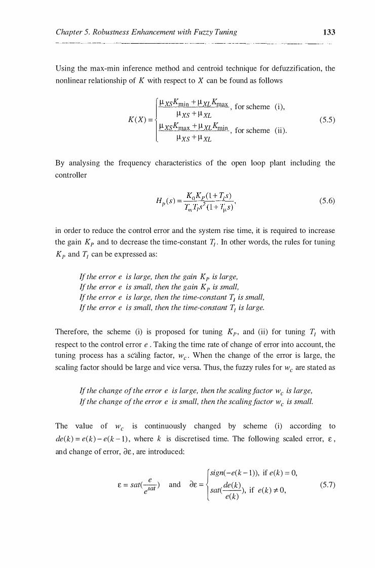
Chapter 5. Robustness Enhancement with Fuzzy Tuning 133 --------------------------------
Using the max-min inference method and centroid technique for defuzzification, the
nonlinear relationship of K with respect to X can be found as follows
K(X) =
1-lxsKmin + llxLKmax , for scheme (i) , llxs + llxL
1-lxsKmax + llxLKmin for scheme (ii) . llxs + llxL
' (5.5)
By analysing the frequency characteristics of the open loop plant including the
controller
(5 .6)
in order to reduce the control error and the system rise time, it is required to increase
the gain K P and to decrease the time-constant T1 . In other words, the rules for tuning
Kp and T1 can be expressed as :
If the error e is large, then the gain K P is large, If the error e is small, then the gain K p is small, If the error e is large, then the time-constant T1 is small, If the error e is small, then the time-constant T1 is large.
Therefore, the scheme (i) is proposed for tuning Kp, and (ii) for tuning T1 with
respect to the control error e . Taking the time rate of change of error into account, the
tuning process has a scaling factor, w c . When the change of the error is large, the
scaling factor should be large and vice versa. Thus, the fuzzy rules for w c are stated as
If the change of the error e is large, then the scaling factor w c is large,
If the change of the error e is small, then the scaling factor w c is small.
The value of w c is continuously changed by scheme (i) according to
de(k) = e(k) - e(k - 1) , where k is discretised time. The following scaled error, £ , and change of error, d£ , are introduced:
e £ = sat( esat ) and
{sign( -e(k - 1)) , if e(k) = 0,
d£ = de(k) . sat(--), If e(k) :;t: 0,
e(k)
(5 .7)

Chapter 5. Robustness Enhancement with Fuzzy Tuning
where { 1, X :2: 1 sat(x) = x, - l :::;; x :::;; 1
-1, X :::;; - 1
134
and esat is the maximum magnitude of the error corresponding to saturation. By
choosing the maximum and minimum values of Kp , T1 and we , the tuning
expressions for Kp and T1 are found as follows (Ha [ 1 12]) :
and
where
(5 . 1 0)
and cr£ and cra10 are some positive constants. The values of TI,nom and KP,nom are
calculated from the nominal values Ko,now Tm,nom ' and Tfl,nom using one of the
symmetrical or magnitude optimum, or other criteria. The prefilter time constant T1 is
set at TI nom .
The simulation parameters of the system K0 , Tm and Til in Figure 5 . 1 are given in
Table 5.2 . The values of TI,nom and Kp are calculated from the values Ko,nom , Tm,nom and Tfl,nom using the symmetrical optimum given in Table 5 . 1 . The prefilter time
constant r1 is set at TI,nom · Choosing the minimum and maximum values for Kp , 0 and we as shown in Table 5 .2, and the coefficients cr10=cra8= 0.0 1 , the controller
parameters are on-line tuned by the following forms
Kp = [2 - 1 . 5exp( -IOO id£ 1)1[8 - 6exp( -1001£ 1) ] , T1 = [2 - 1 . 5 exp( -lOO id£ 1)1[0. 1 + 0 . 3 exp( -100 1£ 1) ] .
Ko,nom Tm,nom Tfl,nom KP,nom rl,nom wc,nom 1 0.4 0.05 4 0.2 1
Table 5 .2. Simulation parameters for tuning PI controller parameters.

Chapter 5. Robustness Enhancement with Fuzzy Tuning 135
The unit step reference response is shown in Figure 5.3 for the nominal case (solid lines) ( Ko = Ko,nom ' Tm = Tm,nom , and T� = T�,nom ) and for a critical case of changing
parameters (dash-dotted lines) (Ko = 0. 5Ko,nom ' Tm = 2Tm,nom ' and T� = 2T�,nom) ,
with fuzzy tuning (curves 1 ) and without fuzzy tuning (curves 2).
1 .4.----------,-----------.-----------.--------�
.... ·- - - - - - -..::... 1 .2
/ _ _ _ ......... _ ___ _ __ _ _ _
I
0 . 8 - ·� I
0.6 I
I
0.4 I KO=KO, nom, I Tm=Tm,nom, Tm=I)l,nom
I 0.2 K0=0.5KO,nom,
Tm=2Tm, nom, 1).t=21).1, nom o��----�--�----------�----------�--------�
0 5 0 1 00 1 5 0 200 tim e, x 0 . 0 1 sec
Figure 5 .3 . Unit step reference response with fuzzy tuning (curves 1 ) and
without fuzzy tuning (curves 2) .
The unit step disturbance response is shown in Figure 5 .4 under the same conditions .
As i t can be seen, a well-damped response with adequately fast dynamics is observed
even in the cases of parameter variation. With fuzzy tuning the disturbance response
exhibits a reduction of approximately 50% in the maximum deviation.
Simulation results indicate that transient performance and disturbance rejection capability are significantly improved with any set of parameters K0 , Tm , and T� given
in the range between half and twice of the nominal values . It should be noted that
fuzzy tuning schemes with different membership functions, such as Gaussian or
sigmoidal, for f.1 xs and f.1 XL can be incorporated in (5.5) instead of exponential
functions. For example, the tuning formulas (5.7-5.9) using Gaussian membership
functions ( 4.28) can be written as

Chapter 5. Robustness Enhancement with Fuzzy Tuning
0.05.-----------�--------�----------�----------�
0 \ -- - --.;. -:_:--
-0.05 1 /
- -�/ /
/
-0.1 /
\ / "
'--0 . 1 5
KO=KO,nom, Tm=Tm,nom, Tm=J1t,nom
_..-____ _
K0=0.5KO,nom, Tm=2Tm,nom, Tf.1=2Tf.1,nom
-0.2 '----------'-------'------'----___:_ _ _:_:_ _ __J
0 5 0 1 00 1 5 0 200
t ime, x 0 . 0 1 sec
136
Figure 5.4. Unit step disturbance response with fuzzy tuning (curves 1) and
without fuzzy tuning (curves 2).
(5. 1 1 )
and
where
(5 . 13)
When using sigmoidal membership functions ( 4.30), the tuning formulas for the
controller parameters are written as :
Kp = wcKP,tun (E) = wJKP,max - 2 (KP,max - KP,min )j(l + exp( - lcl/2crE ))] , (5 . 14)
and
where
(5. 1 6)

Chapter 5. Robustness Enhancement with Fuzzy Tuning 137
PI controllers with fuzzy tuning can be implemented in cascaded controllers for
current, speed, and position loops of drive systems where the problem of changing
parameters and load i s serious. Taking into consideration not only the control error
but also the control signal saturation, the problem of anti-windup (De Vegte [67]) can
also be considered with some fuzzy tuning schemes.
At large values of Tm , we have 1 + Tms = Tms. The closed loop characteristic equation
for the system of Figure 5 . 1 can then be written as follows:
(5 . 1 7)
The stability condition for the system of Figure 5 . 1 is found as T1 > Tfl . Thus, with
fuzzy tuning the overall system is stable if
1/,min > rf.L,max . (5. 1 8)
5.3 Cascade PI controllers with fuzzy tuning
In this section, the proposed PI controllers with fuzzy tuning are applied to flexible
electromechanical structures using cascade control principles. Simulation results
indicate that, with fuzzy tuning, the reference response is well-damped with
adequately fast dynamics and the maximum deviation of the disturbance response is
reduced even in the case of changing plant parameters . The use of cascade PI
controllers with fuzzy tuning increases the capability of vibration suppression in a
multi-mass system, dealing with parameter changes, load disturbance, and backlash
nonlinearity.
5.3. I Overview o.f cascade control
The principles of cascade control, which is quite popular in the field of electrical drives, is illustrated in Figure 5.5, where X1,.�1 , X2,.�f' ' and X3ref are reference inputs to
the first, second, and third loop of the system, respectively. The outputs X1 , X2 , and
X3 can be the current, speed, and position in a drive system. If the plant structure is
known and its parameters are invariant, the parameters of the PI- (or P-) controllers P/1 , P/2 , and P/3 are determined by bringing the open-loop transfer functions into the
approximated form (5 . 1 ) , and then shaping the open-loop frequency characteristics

Chapter 5. Robustness Enhancement with Fuzzy Tuning 138
according to Kessler's symmetric optimum [142] or assigning the closed-loop
characteristic polynomials according to a pole-placement criterion, e.g. magnitude
optimum, Butterworth, or IT AE.
Consider first the symmetric optimum method. Figure 5 .6 shows the desirable Bode
magnitude diagram of the open-loop transfer function after shaping. The 0-dB crossover frequency for such a system is O\: = lj2Tll , and as can be seen, two-fold
symmetry about the ( lj2 Tll , 0 dB) point is observed, thus explaining the symmetric
optimum designation. As remarked by Voda & Landau [ 1 8] , the symmetric optimum
also has an Hoo interpretation.
IHpl (dB)
0
Figure 5 .5 . Multi-loop cascade control.
l !T�-t co
(rad/s)
Figure 5 .6 . Bode plot of the open loop transfer function using symmetric optimum.
In the magnitude optimum method, the design objective is to maintain the magnitude
response curve as flat as close to unity for a large bandwidth as possible (maximally

Chapter 5. Robustness Enhancement with Fuzzy Tuning 139
flat response), for a given plant and cascade controller combination. This 1s
analytically interpreted as follows:
d" ( ) -" IMC.iro)l2 == 0, k = 1 , 2, . . . dro oo=o (5 . 19)
where IMCJro)l is the magnitude closed-loop frequency response. Therefore, the
magnitude optimum technique seeks to eliminate the sensitivity of the magnitude
response to low frequencies. The final closed-loop system characteristic polynomial
results in a practical form:
(5.20)
where l = 1 , 2, 3, . . . . The magnitude optimum technique only optimises the closed-loop
transfer function between the reference input and the variable to be controlled, thus
the system's response due to any disturbance, applied at locations other than at the
reference input, is not optimal.
Two other techniques for determining the controller coefficients are the Butterworth
pole assignment and IT AE methods. The Butterworth pattern is a simple-pole configuration where the n poles, si , ( i == 1 , 2, . . , n ) of the closed-loop system are
equally spaced on a circle of radius ro0 (the system bandwidth) in the left-half plane:
(Re si )2 + (Im si )2 = 1 . ffio2 (5 .21 )
In the IT AE method, the controller coefficients are obtained from the minimisation of
ITAE == min J: tleCt)ldt , (5.22)
where e(t) == 1 - x(t) is the control error, and x(t) is the control output. Appendix A
provides a summary of the normalised characteristic polynomials corresponding to
these methods.
The design with cascade control is quite simple but it has the drawback that the
possibility of any disturbances to the system such as a load torque is ignored and the
approximation (5. 1 ) is not applicable in the presence of uncertainties such as

Chapter 5. Robustness Enhancement with Fuzzy Tuning 140
parameter variations or nonlinearities. It is believed that using the proposed PI
controllers with fuzzy tuning can improve robustness of cascade control systems. In
the following section, a flexible structure system with backlash nonlinearity combined
with the gear torsion is used for simulation.
5.3.2 Application to a two-mass servo drive
Consider the speed control of a two-mass servo system of Figure 3 .3 , reported in Ha
et al. [38 ] . In order to suppress vibration and reject load disturbance in flexible
structure systems, observer-based state feedback techniques with feedforward
compensation have been demonstrated to have significant advantages in comparison
with the conventional PI controllers (Hori et al. [64] or Ha & Negnevitsky [43] . This
problem is addressed here by using the proposed PI-controllers with fuzzy tuning
designed with the principles of magnitude optimum cascade control . Figure 5 .7 shows
the system block diagram with a PI-controller in the current loop and a P-controller in
the speed loop.
current fb
speed fb
armature
back emf constant
Figure 5.7. Two-mass servo system with fuzzy-tuned PI controllers .

Chapter 5. Robustness Enhancement with Fuzzy Tuning 141
Figure 5.8 shows the unit step response of the system without tuning (Figure 5 .8(a))
and with fuzzy tuning (Figure 5 .8(b)) when the load inertia increases to 500% ( ]2 = 5J2 nom).
1
0 . 5
0
1
0 . 5
0
0
0
NWrNww I
I - - - - - - - - � - - - - - - - - - - � - - - - - - - - -
1 I I I I
I I - - - - - - - - - � - - - - - - - - - - � - - - - - - - - -
1 I I I I I
2 0 40 60 Time (sec)
(a)
- - - - - - - - � - - - - - - - - - - � - - - - - - - - -1 I I I I I I
I - - - - - - - - - � - - - - - - - - - - � - - - - - - - - -
1 I I I I I
2 0 40 60 Time (sec)
(b)
Figure 5 .6 . Step response l2 = 512,nom :
(a) without tuning, (b) with fuzzy tuning.
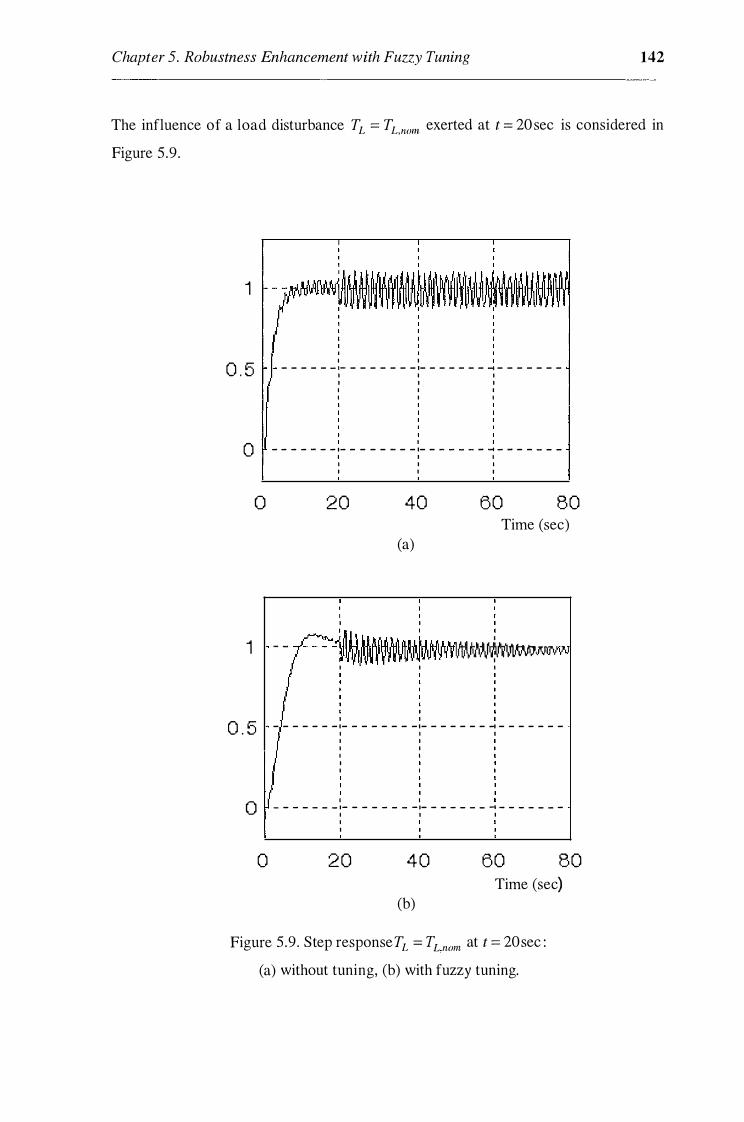
Chapter 5. Robustness Enhancement with Fuzzy Tuning 142
The influence of a load disturbance TL == TL,nom exerted at t == 20 sec is considered in
Figure 5 .9 .
1
0 . 5
0
0
1
0 . 5
0
0
I I
- - - - - _ ,_ - - - - - - - ·- - - - - - - � - - - - - - -I I I I I I I I I I I I
I
- - - - .... - - · - - - - - ..... - - ·- - - - .... .... - _,. - - - -....
- -I I I I I I I I I
20 40 60 80 Time (sec)
(a)
I I I UHJ.MU.tll I'!U � IJo.I..W
I
- - A'III�V���� �YW�VJJ¥� � �I •• WJi;JJWY I I I
I I
- - - - - - - ·- - - - - - - - ·- - - - - - - � - - - - - - -I I I I I I I I I I I
I I
- - - - - - - · - - - - - - - - ·- - - - - - - � - - - - - - -I I I I I
2 0 4 0 60 80 Time (sec)
(b)
Figure 5 .9 . Step responseTL = TL nom at t == 20sec :
(a) without tuning, (b) with fuzzy tuning.

Chapter 5. Robustness Enhancement with Fuzzy Tuning 143
The response with backlash of a dead-band width 2D = 0. 002 is shown in Figure
5 . 1 0.
1
0 . 5
0
0
1
0 . 5
0
0
I - - -rrb�H�\flA�;A�� I
- - - - - - - - � - - - - - - - - - - � - - - - - - - - -1 I I I I I I I
I - - - - - - - - - � - - - - - - - - - - � - - - - - - - - -
1 I I I I I
20 40 60 Time (sec)
(a)
I I - - - - - - - - � - - - - - - - - - - � - - - - - - - - -
- - - - - - - - - � - - - - - - - - - - � - - - - - - - - -1 I
2 0 (b)
I I
4 0 6 0 Time (sec)
Figure 5 . 1 0. Step response with backlash 2D = 0. 002 :
(a) without tuning, (b) with fuzzy tuning.

Chapter 5. Robustness Enhancement with Fuzzy Tuning 144
Comparing the responses in Figures 5 .8 , 5.9, and 5. 10 demonstrates fuzzy tuning can
be applied to cascade controllers in flexible electromechanical systems to increase
robustness to some extent for parameter and load variations, and nonlinearities .
5.4 Sliding mode control with fuzzy tuning
Sliding mode control, b ased on the theory of variable structure systems, first proposed
by Emelyanov [7] in 1 967, has attracted a lot of research on control systems for the
last two decades. The s alient advantage of sliding mode control, developed by Utkin
[8] , is the robust property against structured and unstructured uncertainties . The main
drawback of sliding mode control is the associated undesirable chattering problem
which can excite high frequency unmodelled dynamics. Several methods to reduce
this chattering have been reported, e.g. using a boundary layer in the sliding mode as
in Stoline & Sastry [ 1 52] and Spurgeon [ 1 53], or a continuous sliding mode control
strategy as in Zhou & Fisher [ 1 54] and Nguyen & Nguyen [ 1 55] . The first approach
provides no guarantee for the exact convergence to the sliding mode while the second
tends to produce conservative designs and there is a trade-off between chattering and
robustness. Another method for reducing chattering phenomenon without the sacrifice
of robust performance is to combine the attractive features of sliding mode control
and fuzzy control (Lu & Cheng [ 1 56] and Wang et al. [ 1 57]) .
Fuzzy logic has been proven to be a vigorous tool in ill-defined or parameter-variant
plants. Employing expert's engineering heuristics, a fuzzy logic controller can cope
well with severe uncertainties, however it may suffer from a heavy computational
burden when implemented. Fuzzy tuning with explicit tuners for the controller
parameters can avoid this problem as shown above.
In this section a new technique is presented for linearised systems with uncertainties
using sliding mode control with an additional fuzzy-tuned component to the control
action. The reaching condition in the vicinity of the hyperplane is guaranteed by the
Lyapunov stability method. For accelerating the state trajectories to reach the sliding
hyperplane and compensating for the influence of unmodelled dynamics and
chattering, fuzzy tuning schemes are introduced to continuously change the control
action. Simulation results for a two-mass servo drive demonstrate robust performance
in the presence of parameter and load variations, and backlash nonlinearity.

Chapter 5. Robustness Enhancement with Fuzzy Tuning 145
The linearised model of a dynamic system can be written as:
x = (A + �A)x + (b + �b)u , (5 .23)
where x E Rn is the state vector, u E R is the control signal, A E Rnxn and b E Rn are
the nominal system matrices, and �A and �b are uncertainties. The following
assumptions are made (Ha et al. [22]) :
A l . The uncertainties are continuous matrix functions of the vector of varying system
parameters, p E (}J c RP , where IP is a compact set:
(5 .24)
A2. There exist a vector r(p) E Rn and a scalar h(p) such that the following matching
conditions are satisfied:
�A = brT (p) and max{lr; (P)I} ::;; p , Vp E (}J ,
11b = bh(p) and Jh(p)J :S; cr < l , Vp E (}J . (5 .25)
The objective is to design a controller that provides robust performance in the
presence of uncertainties (5 .24) given their bounds p and cr . In this approach, the
control law is written as :
(5 .26)
where ueq ' u,. , and uft are the control signals for the equivalent motion, reaching phase
with respect to uncertainties (5 .24), and fuzzy tuning to improve control performance, respectively. The control gains k� and k; , and the fuzzy control signal uf1 will be
determined in the following.
5.4. 1 . Robust controller with sliding mode
A sliding-mode controller normally consists of two distinct operating modes: reaching
and sliding. Let us define a switching hyperplane variable:
n S(x) = CT X = �>ixi , (en = 1 ) ,
i=l (5.27)

Chapter 5. Robustness Enhancement with Fuzzy Tuning 146
and the sliding mode
S(x) = 0 or cTx = 0 . (5 .28)
By properly choosing the parameters ci (i = 1, 2, . . . , n ), the desired dynamics of the
closed-loop system can be described by the sliding equation (5.28). Generally, a
sliding mode controller is designed in the sense that, for any initial state x0 = x(t0 ) in
S , the system state x (t) can remain in S for all t > t0 . If x0 is not in S , the controller
can drive the system state x (t) to the sliding mode S(x) = 0 .
A. The equivalent gain and sliding surface
In the sliding mode S(x) = 0 , a necessary condition for the state trajectory to stay on
this hyperplane is S(x) = 0 or:
(5 .29)
The equivalent feedback gain, k!' , can then be expressed as :
(5 .30)
where the existence of the inverse of cTb is a necessary condition. Note that the closed-loop system eigenstructure includes (n - 1) sliding eigenvalues 'Ai (i = 1 ,2, . . . ,n - 1) , and an eigenvalue at the origin of the complex plane 'An = O generated from the condition S(x) = 0 . Thus, the equivalent feedback gain k!' can be
determined by a pole placement technique to assign the desired roots 'Ai ( i = 1 , 2, . . . , n)
to the characteristic equation:
IAI - A + bk!' l = 0 . (5.3 1 )
Vector c in the sliding surface definition (5.28) can then be derived from (5 . 30):
(5 .32)
where the condition (en = 1) in (5 .27) is applied to obtain a possible solution for the
singular equation (5 .32) .

Chapter 5. Robustness Enhancement with Fuzzy Tuning 147
B. The switching gain in reaching mode
Any variations from the nominal system may result in a deviation of the representative
point from the sliding surface. A robust feedback with the switching gain, l\:; , is
developed to meet the reaching condition under which the system state is driven to
reach the sliding surface.
Theorem 5. 1: (Ha [ 1 48]) Consider the linearised system with uncertainties (5.23) satisfying the assumptions Al and A2. If the robust sliding-mode controller is
designed such that
T T u = ueq + ur = -(ke + kr )x , (5.33)
where k� is the equivalent gain given in (5.30) , and k;· is the robust gain to deal with
the system uncertainties, whose i -th element is given by :
_ P + !ke,i lcr , T · -kr i - sgn(c bxiS) , ( t - 1, 2, . . . ,n) , ' 1 - (J
then the state vector x(t) asymptotically converges to zero.
(5.34)
Proof Let us define a positive definite Lyapunov function V = t S2 . For the
occurrence of sliding motion, the trajectories in the neighbourhood of S = 0 must be
directed towards the mode of
lim v ::;; o . S-70
From (5 .23), (5.28), (5 .29) and (5 .33) , we have
S = cr x = cr [(A + L).A)x + (b + L).b )( -k�·x - k; x)] = CT L).Ax - CTbkT X - CT L).bkT X - CT L).bkT X r r e
Thus, the first order derivative of the Lyapunov function can be expressed as :
V = SS = crb[rT (p) - (1 + h(p))k; - h(p)k� ]xS or

Chapter 5. Robustness Enhancement with Fuzzy Tuning 148
n V = �)r; - (l + h)kr,i - hke,d(cTb)x;S . i=l
The condition lim V ::;; 0 will hold if each term of the sum above is non-positive. s�o
Consider first the case ( cTb )x;S > 0 . From (5 .25) we have:
f; - (1 + h)kr,i - hke,i ::;; 0, \ip E (f! if
r - hk . P + alke ; I k > t e,t 1r-1 ill k > , r i - , v p E u� , or r i _ • ' l + h ' 1 - a
Similarly, when (cTb)x;S < 0 , we obtain:
f; - ( 1 + h )kr i - hke ; :2 0, \ip E rP if ' '
< r; - hke,i <
-p - a lke,i I kr i _ , \ip E rP , or kr i _
. ' l + h ' 1 - cr
In the case ( cTb )x;S = 0 , the value of kr i can be chosen to be 0.
In summary, the switching gain can be written as
p + lke i la T k 1· = ' sgn(c bx1.S) ( i = 1 ,2, . . . ,n ) , r, 1 - a {1, X > 0
where sgn(x) = 0, x = 0 . This concludes the proof.
-1 , X < 0
Hence, based on the bounds of uncertain plant parameters, the existence and hitting
conditions of a robust sliding regime are derived and the switching gain is determined
as in (5 .34).
5.4.2. Performance enhancement with fuzzy tuning
In order to accelerate the reaching phase and reduce chattering while maintaining sliding behaviour, an additional control signal, u1r , is introduced:
(5 .35)
Chapter 5. Robustness Enhancement with Fuzzy Tuning 149
This signal is continuously adjusted by the use of fuzzy logic, depending on S defined
in (5.26) and S (Hwang & Lin [1 58]) . From empirical knowledge in the design of
sliding mode controllers, a large switching gain will force the state trajectories to
approach the sliding surface rapidly, but at the same time, tend to excite chattering.
Thus, when the state trajectories are far from the sliding hyperplane, i .e. when the
value of lSI is large, the switching gain should be correspondingly increased and vice
versa. Furthermore, when the state trajectories are deviating from the sliding surface
(SS > 0), if \S\ is large the switching gain should be increased to force the trajectories
back, and vice versa. When the state trajectories are approaching the sliding surface
(SS < 0), if \S\ is large the switching gain should be decreased in order to reduce
chattering, and vice versa. Using simple fuzzy labels large and small for the scaled
modulus of S and S :
. -{sgn( -Sk-I ), if Sk = 0
s* - sk - sk-I k , sat( k ), if S :;t: 0 s
(5 .36)
{sgn(x), lxl > 1 where sat(x) =
I I , Sk is the value of S at t = kT , T is the sampling
X, X < 1
period, the following exponential membership functions are defined (Ha [ 148]) :
1 c s*
) c s* ) !ls_targe = - exp -� , !ls_small = exp -a- '
v s s
. .
s� s* • • - 1 - exp(--) 1 1 - exp(--) �"" !;_large - ' �"" S_small - ' crs crs
(5 .37)
where cr s and cr s are some positive constants . Based on the above discussed
heuristics, the following fuzzy rules are proposed:
(i) If s* is large, then Ws is large,
(ii) If S, is small, then w8 is small,
(iii) If ss > 0 and s* is large, then Utt is large,
(iv) If SS > 0 and s* is small, then u11 is small,
(v) /f SS < 0 and S* is large, then U.tt is small,
(vi) If SS < 0 and s* is small, then u1t is large,

Chapter 5. Robustness Enhancement with Fuzzy Tuning 150
where Ws is a weighting factor depending on S . Singletons are defined as
membership functions for uft and w s :
{1, u./1 = ws {1, u./1 = 0
11u_large = O . -+- ' 11u_small =
0 -+- 0 ' ' u.ft -r- ws ' uti -r-
(5 .38)
where w0 is some scaling factor. Using the centroid defuzzification method for fuzzy
schemes (iii)-(vi) we obtain:
- 11 ,�_large ws + 11 s small 0 - (1
( s* )) uft - - ws - exp -- , SS > 0 .
).l S'_targe + 11 S _small (j S
1-L · o + 11 . w s· _ S_large S small s _ ( * )) SS < O u1. - - w exp -- , . t +
s C5 11 S'_targe 11 Lsmall S
(5.39)
where the weighting factor Ws can be obtained by defuzzifying the schemes (i)-(ii) as
follows:
_ 11s large Wo + 11s small 0 _ (1 (
S* )) Ws - - w0 - exp -- . ).l S_large + 11 S_small C5 S
From (39) and ( 40) the fuzzy control signal u./1 can be written as :
uti =
s� s* w0 (1 -- exp(- -· ))(1 - exp(--· )), SS > O
O's cr,�
w0 (1 - exp(- �)) exp(-�), SS < O O's as
where w0 , a8 and as are three parameters of the tuner.
(5.40)
(5.41)
As an illustrative example, the proposed technique is applied to the design of a robust
controller for a two-mass servo drive system with backlash nonlinearity in the

Chapter 5. Robustness Enhancement with Fuzzy Tuning 151
coupling shaft gear (Ha et al. [22]) . The plant model and specifications were given in
Figure 5 .7 . The linearised state model of the plant can be written as :
Tm -33. 3 - a 0 0 �n a 0
(J)l 1 . 23 0 1 . 23 0 (J)l 0 0 = + (J)r�f' + TL
112 0 0. 2 1 0 - 0.2 1 112 0 0
(J)2 0 0 83 .3 0 (J)2 0 -83. 3
where �n' ro1 , 11 2 and ro2 are the motor torque, motor speed, elastic torque and load
speed, respectively, ffiref and TL are the reference input and external load torque,
a = 237. 3 ± 1 1 8 . 7 is an uncertain element depending on the stiffness of the drive
speed-torque characteristics. The hyperplane eigenvalues are chosen to be
A-1 2 3 = [ - 1 1 - 1 1 - 1 1] . The equivalent feedback gain obtained by a pole placement
technique is found to be k�q = [ -0. 0074 0. 0789 9. 8844 - 1. 0789] . The parameters
for the sliding surface are obtained from (5.32) as cr = [0. 035 0 . 924 44. 843 1] . The
switching gain k;: is calculated from (5.34) and the tuner parameters are chosen to be
w0 = 6 , cr s = 0. 5 , and cr s = 0. 0 1 . The step response of the load speed as the system
output is shown in Figures 5 . 1 1 , 5 . 1 2, and 5 . 13 for the cases of a constant load torque
TL exerted at t = 5 sec , backlash with a dead band width of 2D = 0. 03 , and a 50%
reduction of the drive stiffness with 2D = 0. 0 1 and a load torque, respectively . It is observed that sliding mode control can cope well with nonlinearity and parameter
variation, but cannot achieve load-insensitivity .
Comparing with the responses obtained by pole placement (Figures 5 . 1 3(a)), sliding
mode control without tuning (Figure 5 . 13 (b)) indicates that an additional fuzzy tuner
inherently improves system robustness against load torque disturbance (Figures
5 . 1 3 (c)) without the sacrifice of good sliding behaviour.
5.5 Summary and further discussion
In this chapter, simple fuzzy tuning schemes are introduced to continuously change
the controller parameters or the control action in order to enhance robustness. The
gain and time constant of a conventional PI controller are made continuously changed
by some exponential functions, resulting from some engineering heuristics with the
use of fuzzy logic. System robustness is verified through high performance of
transient responses in changing environment conditions. Explicit expressions for the
controller parameters facilitate the tuning process at a low computational cost.

Chapter 5. Robustness Enhancement with Fuzzy Tuning
1 - - -,.....------< - - - - - - - - - - - - - - - - - -
0 .5 - - - - - - - - - - - - - - - - - - - - - - - - - - - - - - - - - - -
0 - - - - - - - - - - - - - - - - - - - - - - - - - - - - - - - - - - - -:
0 5 1 0
0 .5
Time (sec) (a)
' � - - - - � - - - - - - - - - - - - - - - - - - .... - -- - -- - - � - -- - - � - -- .. -- - - - - -' ' '
' 0 - - - -- - - - - - - - - - - - - - -- - -- - - : - - - - - - - - - - -- - - - - - - - - - - - - - -
'
0 5 1 0 Time (sec)
(b)
1 - - - - - - - -- - - - - -,.-.- -�--- -- - - - - - - - - - -:_:.;--,...---..........,
0 .5 ' - - - - _ _ _ _ _ _ _ _ _ _ _ _ _ _ _ _ _ _ _ _ _ .. _ _ _ _ _ _ _ _ _ _ _ _ _ _ _ _ _ _ _ _ _ _ _ _ _ _ ' ' ' ' ' '
' 0 - - - - - - - - - - - - - - - - - - - - - - - - - � - - - - -- - - - - - - - -- - -- - - - - - - - -
0 5 1 0 Time (sec)
(c)
Figure 5 . 1 1 . Step response with a load torque exerted at t = 5 sec .
152

Chapter 5. Robustness Enhancement with Fuzzy Tuning
0 . 5
- - - _-:::-:, - - -
8 � - - - - - - - - - - - - - - - - - - - - - - -"' - - - - - - - - - - - - - - - - - - - -- - - - - -' '
0 - - - - - - - - - - - - - - - - - - - - - - - - - - : - - - - - - - - - - - - - - - - - - - - - - - - - -
0
' '
5
(a)
1 0
Time (sec)
1 - - - - - - - - - - - - - -- ::_:;- - -:,::..:- -,.:...- • _.;--___ �.............,
0 . 5 ' - - - - - - - - - - - - - - - - - - - - - - - - - .I - - - - - - - - - - - - - - - - - - - - - - - - - -
' ' ' ' '
' 0 - - - - - - - - - -- - - - - -- - - - - - - - -: - -- - - - - - - - -- - -- - - - - - - - - - - -
0
' '
5
(b)
1 0 Time (sec)
1 - - - - - - - - - - - - -,--..--;...---�--=- =- - =- - ·:..:..:j·
0 .5 ' - - - - -- - - - - - - - - - -- - - - - - - - - � - - - - -- - - - - -- - -- - - - - - - - - - - -' ' ' ' ' ' ' ' 0 - - - - - - - - - - - - - - - - - - - - - - - - - : - - - - -- - - - - -- - - - - -- - - - - - - - -
0
'
5
(c)
1 0 Time (sec)
Figure 5 . 1 2. Step response with backlash 2D = 0. 03 .
153
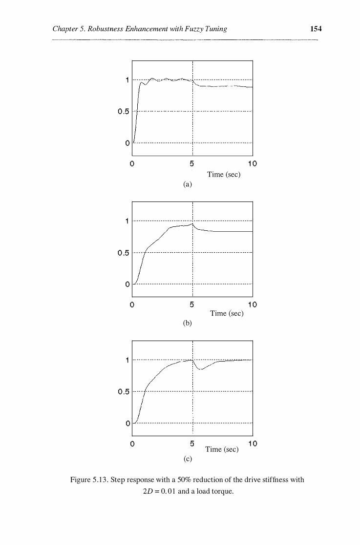
Chapter 5. Robustness Enhancement with Fuzzy Tuning
1 - - - - - - - - -- � - - - - - - - - -- - - - - - - - - - - - - - - - - -
0 .5
; ----------1 ' ' ' ' M - M �N � -- � WW M -- � MM M MM W MM M a .l p WM M - - M MM M -� M - - - MM M - - M MM � M
0 l _ _ - - - - - - - - - - - - - - - - - - - - - - . ; - - - - - - - - - - - - - - - - - - - - - - - - -
' ' '
0 5 1 0 Time (sec)
(a)
1 · - - - - - - - - - - - - - - - - - - - - - - - - - . , - - - - - - - - - - - - - - - - - - - - - - - - - -
0 .5 - - - - - - - - - - - - - - - - - - - - - - - _ ., _ - - - - - - - - - - - - - - - - - - - - - - - - -' '
' 0 - - - - - - - - - - - - - - - - - - - - - - - - - : - - - - - - - - - - -- - - - - - - - - - - -- - -
0 5 1 0 Time (sec)
(b)
1 - -- - -- - -- - -- - -- - -- - -- - - - - - - - - - -- - - - - - - - - - - - - - - - -
0 .5 ' - - - - - - - - - - - - - - - - - - - - - - - - _ , - - - - - - - - - - - - - - - - - - - - - - - - - -'
' 0 - - - -- - - - - -- - - - - -- - - - - - - - - : - - - - -- - -- - - - - - - - -- - - - - -- - -
0
' '
5
(c)
1 0 Time (sec)
Figure 5 . 1 3 . Step response with a 50% reduction of the drive stiffness with
2D = 0. 0 1 and a load torque.
154

Chapter 5. Robustness Enhancement with Fuzzy Tuning 155
The results can be extended to multi-loop cascade control . In each loop, a PI
controller with fuzzy tuning is used instead of a conventional one. Simulation results
in a two-mass system indicate that fuzzy tuning can be applied to cascade controllers
in flexible electromechanical systems to increase robustness to some extent for
parameter and load variations, and nonlinearities.
In Section 5.4, fuzzy schemes are applied to tune not the controller parameters but the
control action itself to deal with unmodelled dynamics in sliding mode control . This
technique combines the features of sliding mode control and fuzzy control. First, the
equivalent motion is determined from the desired sliding eigenstructure. The reaching
condition in the neighbourhood of the sliding surface is satisfied by the use of a
switching gain based on the Lyapunov stability theory. Fuzzy tuning schemes are then
employed to accelerate the reaching phase, reduce chattering, and hence, improve
robust performance. The proposed technique can be applied to the control of a elastic
drive system. Simulation results in a servo two-mass drive demonstrate its validity.
Again, the explicit expressions for fuzzy schemes facilitate the computational
implementation of the proposed controller.
Fuzzy tuning of the PI controller parameters has demonstrated the capability of
improving system robustness to parameter and load variations, and nonlinearities in
motion control systems. Moreover, windup is an inherent problem that should be
taken into account due to integrator saturation, especially in process control. In order
to cope with these types of nonlinearites the design method should be adjusted with
some ad hoc fix anti-windup. This anti-windup is normally designed to prevent the
integrator state in the controller to become too large. The idea is to decrease the rate
of change of the integrator state when the control error is large for a longer period of
time. Utilising not only the control error but also the control signal saturation,
Hansson et al. [ 1 60] proposed anti-windup schemes with fuzzy tuning for controllers
applied in the control of a double tank. Fuzzy tuning may also be implemented in
other control strategies with the purpose of robustness enhancement. In particular,
proportional-derivative (PD) controllers provide high sensitivity and tend to increase
the stability of overall feedback control system. In addition, PD controllers can reduce
overshoot and increase damping capability of the system. It has been proven that a PD
controller can show its effectiveness in low-order systems, but usually can hardly be
suitable for higher-order and nonlinear systems. Malki et al. [ 1 59] demonstrate that
fuzzy PD controllers, where the control output depends on the error and its derivative

Chapter 5. Robustness Enhancement with Fuzzy Tuning 156
as in ( 4.45), have some remarkable advantages over conventional one. It is worth to
elaborate on some fuzzy tuning schemes to extend the application of PD controllers to
high order systems and improve robust performance in the comparison with
conventional PD controllers.
While sliding mode control guarantees system invariance under parameter variations,
it has one major disadvantage - unmodelled dynamics or chattering. In most industrial
applications, the ideal sliding mode is smoothed by introducing a bounder layer
containing the sliding hyperplane. Thus, "soft" sliding control with a boundary layer
(Stoline & Li [ 16 1 ]) leads to the possibility of selecting the layer thickness which can
be tuned experimentally, based on engineering experience and judgment. This
justifies the use of an additional component in the control law (5.35). Further research
in sliding mode control with fuzzy tuning may result in a simpler control law
consisting of two signals or even one signal because, essentially, fuzzy logic control is
also a variable structure system (Yager & Filev [1 30]) .
Conventional proportional-integral-derivative (PID) controllers in various
combinations have been widely used for industrial processes due to their simplicity
and effectiveness for l inear systems. Thus it is of importance to have good tuning
algorithms for these controllers. Scaling factors for the controller parameters can be
introduced and rules can be derived to update these factors, in dependence on the
performance of the closed loop system, and utilising the known strategies for tuning
PID controller parameters. In general, the criteria for tuning are based on the values of
the transient response overshoot, settling time, and amplitude of oscillation. For
example, a prototype rule set for tuning PI controller parameters are given in Section
5 .2 . It is straightforward to extend the approach to other conventional controllers. In
the following chapter it is applied to robust modal control described in Chapter 3 .

Chapter 6
Robust Modal Control with Fuzzy Tuning
In Chapter 3, robust modal control has demonstrated the capability of providing high
performance response for electromechanical systems with flexible structures.
However, the observer and feedforward compensator are designed on the basis of
system nominal parameters . Consequently, parametric robustness of the whole system
has not completely achieved. This chapter employs tuning schemes, heuristically
inferred with fuzzy logic, to improve invariant performance of robust modal
controllers.
6.1 Introduction
In high performance position drive applications, it is required to develop a controller
that can provide high positioning accuracy, fast dynamic response and insensitivity to
any perturbations , such as load torque disturbance, parameter variations, nonlinear
friction, etc. A great majority of position drives in industry utilise DC-motors with a
cascade controller consisting of a PI-current controller loop, a PID-velocity controller
loop and a P- (or PI-) position controller loop. Although cascade control design is
simple and straightforward, there are trade-offs in achieving all the performance
requirements . The adaptive controller is effective in drive systems with an uncertain
parameter model but it gives undesirable responses (Dote [65]) . The variable structure
system control is insensitive to variations of the drive system but chattering
phenomenon is a problem and in some cases the sliding mode does not exist (Furuta
[7 1 ]) . There have been many formalised approaches to improve robustness of position
drive system [ 1 62 , 7 8 , 64, 19] . The robust model matching principle in Eisaka et al.
[ 1 62] is based on zeroing the transfer function from the equivalent disturbances to the
controlled output. The feedforward compensation is used in Ko et al. [78] and Hori et
al. [64] to provide quick and effective results for reduction of motor speed fluctuation

Chapter 6. Robust Modal Control with Fuzzy Tuning 158
due to load variations . However, the parameter-insensitivity of the overall drive
system has not been considered.
Robust modal control has been elaborated (Chapter 3) to improve the performance of
the system subject to both load and parameter variations. The modal controller applies
full state feedback from the drive state variables. A predictive observer (Alferov & Ha
[73]) is used to estimate simultaneously the external disturbance and the states not
directly measurable. To obtain load-insensitivity, the modal control signal is
feedforward compensated from the estimated disturbance. To deal with the problem
of parameter variation, a robust control signal is added to the modal control signal.
The asymptotic stability of the overall system with parameter uncertainty is
guaranteed by the second method of Lyapunov. While robust modal control can give
desirable dynamic and static performance of the drive system in the presence of load
disturbance, the observer is still sensitive to parameter variation and the step response
rise time at nominal parameters is slightly slower than the rise time in standard modal
control. This can be explained by the fact that all the controller coefficients were set
constant (see, e.g. Ha & Alferov [ 1 9]) . This chapter focuses on using fuzzy logic
schemes to tune the observer predictive coefficients, the feedforward gain and the
robust feedback gain. As described in Chapter 4, fuzzy logic control has recently
arisen as a powerful approach to deal with uncertainty. Tuning the controller
coefficients to achieve robust tracking i s non-trivial . The simulation results indicate
that by fuzzy tuning the controller coefficients, the drive system is made more robust
to load and parameter variations without loss of performance at the system's nominal
parameters . Exponential, sigmoidal , and Gaussian can be used for membership
functions in fuzzy rule set. The material of this chapter is based mainly on the studies
by Ha [39, 40] , Ha & Negnevitsky [2 1 , 37, 4 1 , 42, 43] , and Ha & Palis [ 1 63] .
6.2 Digital predictive observer with fuzzy tuning
In robust modal control, it is required to estimate the state variables that are not
directly measurable for state feedback, as well as the unknown inputs for their
compensation. such as load torque also needs to be estimated for rejection purposes in .,
order to increase the system robustness. Designing observers that are capable of
simultaneously estimating state variables and unknown inputs becomes of interest. In
Park & Stein [97], the state equation is transformed into a special system model for a
reduced-order observer. The design procedure in Alferov & Ha [73] is straightforward

Chapter 6. Robust Modal Control with Fuzzy Tuning 159
with the introduction of a predictive coefficient to approximate the unknown input.
However, the predictive coefficient was set to be constant.
In this section, the proposed approach is generalised and the observer robustness is
improved by tuning the predictive coefficients, taking into account the disturbance
rate of change. The observer performance is verified through an illustrative example
of a two-mass position drive (Ha [39]) . Not restricted to motion control, the proposed
observer can be applied, in terms of the estimated states, to obtain the parameter
trajectories in order to detect incipient faults, as described in Ha & Negnevitsky [43] .
Consider a linear time invariant dynamic system described by the following discrete
time state equation:
x(k + 1) = Ax(k) + Bu(k) + Dv(k)
y(k) = Cx(k) (6 . 1 )
where x(k) E Rn is the state vector, u(k) E Rr is the control vector, v(k) E Rq is the
disturbance vector, and y(k) E Rm is the output vector the system, respectively. The
matrices A E Rnxn , B E Rnxr , C E Rmxn , and D E Rnxq are constant matrices subject
to parametric uncertainties.
Following the design approach described in Section 3.4.2, we obtain a combined
observer for state and disturbance estimation with the state equation given in (3.76). The observer response depends the choice of matrix r = diag( y ii ) of predictive
coefficients "fu , i = 1, 2, . . . , q . For given predictive coefficients Yu = 'Yiio , there usually
exists a proper choice of the matrix gain L1 , L2 such that desirable observer
dynamics can be obtained. If the unknown inputs vary slowly with time and there is no deviation in system parameters from their nominal values, 'Yuo can be set equal 0.
In practice, the rate of change of unknown inputs is uncertain and the system is
subject to parameter variations.
Inspired by fuzzy tuning schemes discussed in Chapter 5, it is worth improving
robustness the proposed observer by continuously changing the predictive coefficients. In Ha [39], 'Yii is made continuously changed by the use of fuzzy logic so
that the approximation in Equation (6) is tuned with respect to the rate of change of
Vi· Note that if modulus of the change of the estimated unknown input vi is large, then
the corresponding predictive coefficients Yu should be kept small in order to
guarantee smoothness and thus , robustness. By defining

Chapter 6. Robust Modal Control with Fuzzy Tuning
where { 1 , X > 0
sign(x) = 0, x = 0
-1, X < 0
{ 1, X ;?:?: 1
, and sat(x) = x, - 1 < x < 1 ,
-1, X � -1
the following simple rules are then introduced:
if ri is large, then Yu is small.
if r; is small, then Yii is large.
160
(6.2)
The typical membership functions for ri and Yu can be shown in Figure 6. 1 . A given
value of ri can be fuzzified as having J..L1 grade small and J..L2 grade large. The
predictive coefficient Yu at the k-th sampling is then inferred by the well-known max
min rule and the centroid method, described in Chapter 4:
Figure 6. 1. Membership functions for ri and Yii '

Chapter 6. Robust Modal Control with Fuzzy Tuning 161
(6.3)
where �1 and Yii (�2 and yi2 ) are the membership grade and crisp value of Yu
corresponding to the fuzzy set r; is small (large) .
As scheme (ii) (see Section 5 .2) is used for inferring the predictive coefficients 'Yii ' when using exponential membership function for ri and singleton for Yu as in (5 .3)
and (5 .4) :
and
{1, Yii = 'Yii,m �large ( 'Yii ) = O, 'Yii 1:- 'Y ii,m
the value of Yu can be obtained from (5.5) or (6.3) as in Ha & Negnevitsky [37] :
'Yii = 'Yii,m exp( -h l/cr'i ) , where 'Yii m and cr" are some positive constants . ' l
The design procedure can be included in the following steps:
(6.4a)
(6.4b)
(6.5)
Step] : Find the discrete-time state equation (6 . 1 ) describing the system with unknown
inputs. Obtain the matrix blocks of the augmented form (3 .75).
Step2: Choose the observer matrix gain L1 , L2 . For given matrix of predictive coefficients r0 , determine the elements lu for the observer desired dynamics.
Step3: Define membership functions for the rate of change ri and coefficient y ii . Tune
'Yii in the approximation (3 .74) by the defuzzification formula (6.3) of by fuzzy tuning
expression (6.5) .
Example 6. 1 : Consider again Example 3.3 of a DC motor two-mass electromechanical
system of Figure 3.3 . The block diagram with specifications is also in Figure 3 .5 . The
elaboration of Step 1 and Step 2 is described in Example 3 .3 . In Step3, the predictive
coefficient y in the approximation

Chapter 6. Robust Modal Control with Fuzzy Tuning 162
TL (k + 1) = (1 + y) TL (k) - yTL (k - 1)
is made changing in dependence of the normalised rate of change of estimated load
torque r(k) defined in (6.2). Exponential and singleton membership functions (6.4)
are assigned to the rate of change r(k) and y , respectively. Thus, tuning expression
for the predictive coefficient y can be obtained from (6.5) as y = y me-alrl , where y m is some constant and 0' is positive. The nonlinear relationship between y and r can be
represented in Figure 6 .2. The realisation schematic diagram of the proposed digital
predictive observer (DPO) is presented in Figure 6.3 .
Figure 6.2 . Nonlinear y with respect to r.
, - - - - - - - - - - - - - - 1 u I
I i
a
Figure 6 .3 . DPO schematic diagram.

Chapter 6. Robust Modal Control with Fuzzy Tuning 163
To suppress elastic mechanical vibration and achieve load- and parameter
insensitivity in this system (Figure 3 .5), a robust controller described in Example 3 .7
is used with feedback from the measurable and estimated state variables and
feedforward from the estimated load torque. With tuned predictive coefficient y = 0. se-O . l r (y m= 0.5 and 0'= 0. 1 ), Figures 6.4(a) and 6.4(b) show the actual (dotted
line) and estimated (solid line) load torque when the unknown input varies stepwise
and sinusoidally at nominal values of the plant parameters. The actual and estimated
elastic torque are shown in Figure 6.5 when TL varies stepwise. Note that in the
simulation, the observer initial state variables are set at ( 1 , 1 ) as in Example 3.3 . The
results indicate that the proposed digital predictive observer with fuzzy tuning is
capable of producing correct estimates when the unknown input is time-varying.
1 . 2 .-----�--�--�-----,
0.8
E � 0.6
:::; 0.4 f-
0.2
0 1'------�
· · · · ·· · · ·· ·· ·· ·· · ··y----
-0 .2 '----�----,-":-::-----:-":-::------,:-' 0 50 1 00 1 50 200
time. x 0.05sec
(a)
0.8
0.6 E 0 � 0.4 . -
-' f-
0.2
0
-0.20 50 1 00 1 50
time. x 0.05sec
(b)
200
Figure 6.4. Actual and estimated load torque: (a) stepwise, and (b) sinusoidal.
2
1 . 5
E 0 t: 1-(!) 1-
-0.5
-1 0 50 1 00 1 50 200
time. x 0.05sec
Figure 6.5 . Actual and estimated elastic torque when TL varies stepwise.

Chapter 6. Robust Modal Control with Fuzzy Tuning 164
To demonstrate the observer robustness, Figure 6.6 depicts the actual and estimated load torque when the load moment of inertia 12 increases to 12= 5 12,nom CJ2,nom=
0.0 1 2 kgm2) without tuning y (Figure 6.6(a)) and with tuned y (Figure 6.6(b)). Step
response of the closed-loop system with robust modal control using the proposed observer is shown in Figure 6.7 when TL varies stepwise and 12= 5 12,nom · Comparing
Figures 6.6(a) and 6.6(b), and Figures 3 .6 and 6.4 shows that fuzzy tuning makes the
observer less sensitive to system parameter variations without affecting observer
performance at nominal parameters . Similar conclusions can be derived when using
fuzzy tuning in the case of unavailable load speed measurement (see Example 3 .3)
(Ha [39]).
E 0 !:: t::: .....J 1-
E 0 0 � .....J 1- - 1
-2
-3 �--�----�----�----�----� 0 200 400 600 800 1 000
1 . 5
0 .5
-0.5
-1
-1 .5 0 200
time. x 0.05sec
(a)
400 600 time. x 0.05sec
(b)
800 1 000
Figure 6.6 . Actual and estimated load torque at 12 = 512,nom :
(a) without tuning, and (b) with fuzzy tuning.

Chapter 6. Robust Modal Control with Fuzzy Tuning 165
1 . 2 r---,-----,-----,-----,----,
0 . 8 ('IS � 0 . 6
0.4
0 . 2
200 400 600 800 1 000 time. x 0 .05sec
Figure 6.7. Position output step response when TL varies stepwise and 12 = 512,nom .
A simple and straightforward approach for designing digital predictive observers
(DPO) with fuzzy tuning has been presented. This observer is used for simultaneously
estimating the unmeasurable state variables and unknown inputs. The observer is
capable of providing correct estimates when the unknown inputs are time-varying.
The rate of change of disturbances is taken into account by changing the predictive
coefficient with the use of an explicit fuzzy scheme. Thus, the observer is made more
robust to system parameter variations and the tuning is easy. The simulation
demonstrates that the proposed observer can be used with a robust modal controller to
suppress vibration and reject load disturbance influences in multi-mass
electromechanical systems. Its application can also be found in incipient fault
detection in power systems as given in Ha & Negnevitsky [43] (see Appendix B).
6.3 Feedforward controller with fuzzy tuning
In the observer-based controllers discussed in Section 3 .5 , the load torque TL was
assumed to be constant. However, an equivalent unknown load torque to servo
systems can be time-varying and thus, a dynamic compensation for its influence is
required. In this section the time rate of change of TL is also considered taking into
account the uncertainty in variations of friction, load, and parameters . Dynamic
feedforward controller is introduced to compensate for the load torque and its rate of
change, which can be estimated using a digital predictive observer described above.
Here, the feedforward gain is continuously changed by fuzzy logic, dependent on the
magnitude and rate of change of motion error. Thus, the drive system is made more

Chapter 6. Robust Modal Control with Fuzzy Tuning 166
robust to any perturbations . Simulation results are provided for the cases of one-mass
and two-mass position drives .
The basic equation for electric drives is given by
dm Tm = ] - + Bm + TL ,
dt (6.6)
where T:n, m , J , B , and TL are the motor electromagnetic torque, speed, moment of
inertia, viscous friction coefficient and load torque, respectively. Variations in generating torque 1'1Tm , moment of inertia M , friction 118 can be equivalently referred
to as an uncertain load torque change 11TL :
(6.7)
Servo drives with several types of motors can then be modelled in the discrete-time
state space under linearised conditions by the following equation (Ha & Alferov
[ 1 9]) :
x(k + 1) = Ax(k) + Bu(k) + DTL (k)
y(k) = (lm O)x(k), (6.8)
where x(k) E Rn is the drive state vector (position, velocity, current, supply voltage,
etc .) , u(k) E R is the control signal, TL (k) E R is the external disturbance to the drive
system, y(k) E Rm is the output vector, Im is the m x m identity matrix, and A , B, D
are constant matrices with dimensions n x n , n x 1 , n x 1 , respectively. The proposed
dynamic feedforward controller will be constructed on the basis of a disturbance
observer. A digital predictive observer (DPO) is proposed in Section 3 .3 for
simultaneous estimation of the unknown inputs and state variables which are not
directly measurable. To improve observer robustness a fuzzy logic scheme is
introduced to tune the predictive coefficients as described in the section above.
The discrete-time control signal u(k) with full state feedback and observer-based
feedforward compensation (Ohishi et al. [99], Ko et al. [78] , Ha & Alferov [ 1 9] , Yori
et al. [64]) can then be written as
(6.9)

Chapter 6. Robust Modal Control with Fuzzy Tuning 167
where Ur�f' is the reference input which is a step value as in a tracking servo problem,
um (k) = -Kmx(k) is the feedback signal from the drive state x(k) , and uf (k) is the
feedforward compensation signal. An unknown load torque Tr, (k) , in general, can be
considered as a combination a slowly time-varying component Tr,o and a perturbation
component Tr,kT dependent on its time derivative Tr, (T is the sampling period). The
feedforward signal will then consist of a static signal u1;, and dynamic signal u1d :
uf ( k) = ur� ( k) + u1d ( k) = Kr1• Tr, ( k) + Kfd ( Tr, ( k) - Tr, ( k - 1)) , (6. 1 0)
where K1s and K1d are found from the condition of zero steady state error with
respect to a constant and ramp disturbance input, and Tr, ( k) is the estimate of the load
torque obtained from a disturbance observer.
6.3. 1 One-mass servo drive
The block diagram of the observer-based feedforward controller for an one-mass
servo drive is shown in Figure 6.8 (Ha [40]) . The unknown input 7� (k) is estimated
by the observer DPO. When the load torque is constant, the static feedforward gain Kr� is determined from the condition of zero steady-state error (the motor speed
CD = 0 , current ia = Tr,j Kt , supply voltage esp = Tr,Ra/ Kt , control voltage
u = Tr,Ra/CKtKsp ) , and error ess = 0):
Controller
I i cfk)
{J) (k) I e(k)
Figure 6.8. Feedforward controller block diagram for one-mass position drives .

Chapter 6. Robust Modal Control with Fuzzy Tuning 168
(6 . 1 1 )
where Ra and K1 are the motor armature resistance and torque constant, Ksp is the
supply amplifier gain, Kes and Kia are the supply voltage and current feedback gain.
The dynamic feedforward gain is found in the same way with a ramp load torque
TL (t) = tLt .
In the steady-state tracking regime, the motor speed co = 0 , current
supply voltage esp = Ra TL ( Ta + t) / Kl ' and control
u = Ra TL (Ta + T.vp + t) / K1 Ksp . Thus, the condition ess = 0 with
iL = (TL (k) - TL (k - 1) )/T gives
ia = TLt/K1 ,
voltage
t = kT and
(6. 12)
where Ta and T.vp are the motor armature and supply amplifier time-constants.
6.3.2 Two-mass servo drive
The block diagram of the observer-based feedforward controller for two-mass servo
drives (Hori et al. [64]) is shown in Figure 6.9. Here the load torque TL (k) as an
unknown input, and the load speed co2 (k) and elastic torque � (k) as the states, which
are not directly measurable, will be estimated. For the case of a two-mass servo drive,
the static feedforward coefficient is found as in the former case (the motor and load speed co1 = co2 = 0 , elastic torque � = TL , current ia = TL/ K1 , supply voltage
e1P = TLRa/ K1 , control voltage esp = TLRa/ K1Ksp , and error ess = 0):
(6. 1 3)
where Kre is the elastic torque feedback gain. With TL (t) = TLt as a ramp input, the
zero steady-state tracking error requires the load speed co2 = 0 , motor speed
co1 = tL/K1 2 , elastic torque � = TLt , current ia = T1J/K1 , supply voltage
e1P = (Kb / K12 + Ra (Ta + t)j K1 )TL , and control voltage u = esp j Ksp . The dynamic
feedforward gain in this case is found to be
Ktd = Kdo + Kt:�k,
Kdo = (KesRa1� j K1 + Ra CTa + T.�p )j KspKt + Kbj KspKI2 + (KesKb + Kro1 )/ K12 )jT (6. 1 4)

Chapter 6. Robust Modal Control with Fuzzy Tuning 169
Figure 6.9 . Feedforward controller block diagram for two-mass position drives.
where Kw1 is the motor speed feedback gain, Kb is the motor back emf constant, and
K12 is the coupling rigidity modulus.
6.3.3 Fuzzy logic tuning
While feedforward gains in Equations (6. 1 1 )-(6 . 14) are defined at the system nominal
parameters the compensation in Equation (6. 1 0) is still sensitive to parameter
variations. To improve the robustness of the servo accuracy, a fuzzy tuning scheme is
proposed. Fuzzy logic has been proposed to tune the coefficients of PI-controllers in
the previous chapter. It is believed that the idea of fuzzy logic tuning can be extended
to more complex controllers, benefiting directly from human engineering experience.
Here the dynamic feedforward coefficients will be tuned according to knowledge of the control error and the estimated load torque. By denoting e = Sr�f' - 8 , where 8,4 and 8 are the reference and actual output of the position drive, the error modulus is
reflected by {I e(.k) I �f ie( k Jl ::; \esat \
E(k) = esat 1, otherwise,
(6. 15)

Chapter 6. Robust Modal Control with Fuzzy Tuning 170
where esat is the maximal magnitude of the control error corresponding to saturation
of the servo power amplifier. The following conditional scheme is provided for
continuously changing the dynamic feedforward gain, dependent on the signs of e( k)
and dTL (k) = TL (k) - �� (k - 1) :
IfSDTESE and EL then KDL, If SDTESE and ES then KDS,
If SDTNESE and ES then KDZ, If SDTNESE and EL then KDN,
where the labels EL, ES, KDL, KDS, KDZ, KDN, SDTESE, and SDTNESE mean E(k) is large, E(k) is small, K1d is large, Kfd is small, K
.fd is zero, Kfd is negative,
sign( dTL ) = sign( e) , and sign( dTL ) ::f. sign( e) , respectively. By defining the
corresponding membership functions as
{ 1, sign(dTL ) = sign( e) {1 , sign(dTL ) ::f. sign( e) 11 SDTESE = A ' 11 SDTNESE = A '
0, sign(dTL ) ::f. sign(e) 0, sign(dTL ) = sign(e)
1 - <J E - <J E 11EL = - e r ' 11ES = e r
{1 , Kfd = 2Kdo {1, K1d = Kdo flKDL = ' 11KDS = '
0, K.fd ::f. 2Kdo 0, K1d ::f. Kdo
{1, K.fd = 0 11 KDZ =
0, Kfd ::f. 0 ' {1, Kfd = -
Kdo 11KDN = '
0, Ktd ::f. Kdo
(6. 16)
the value of K1d is found by the max-min inference and centroid method (Ha [40]) :
(6. 17)
The explicit form of the above equation provides an easy tuning for the controller
coefficient and thus results in a cheap computational implementation.
Example 6.2 (Ha [40] ) Consider first the one-mass servo system of the radial arm
motion of an ABB robot using a DC motor F12M4 (43V, 240W, 3000 r/min) supplied
by a PWM transistor chopper. The block diagram of the servo system with cascade
controllers (PI-current regulator, PID-speed regulator and P-position regulator) is
shown in Figure 6. 10 .

Chapter 6. Robust Modal Control with Fuzzy Tuning 171
Figure 6. 1 0. Block diagram of a one-mass system with a cascade controller.
The parameter nomenclature and nominal specifications are listed in Table 6. 1 . The
controller parameters are given in Table 6.2. Experiments and simulations indicate
that with cascade control, the third pattern motion (to and fro along x-axis) of the
robot is sensitive to l oad and inertia variations. Figure 6 . 1 1 depicts the voltage
waveform corresponding to the x-axis position of the robot when moment of inertia
J = 2Jnom ·
An observer-based feedforward controller described above is proposed. The sampling
period is T = 1ms . The ITAE criteria is used for pole placement with base frequency chosen as ffin= 47 radlsec (steady-state time 0. 1 sec, overshoot 10%). The feedback
gain obtained, kT = (K8 Kes Kia Kr J together with the values of feedforward
coefficients K.fs and Kdo according to Equations (5,6) are given in Table 6 .3 .
Parameter Value
Supply amplifier gain, Ksp 10 Supply amplifier time constant, T.vp 0.01 (ms) Armature resistance, Ra 0.93 (ohm) Electromagnetic time constant, Ta 0.03 (sec) Back-EMF constant, Kb 0. 1 1 (V/sec- 1 ) Torque constant, K1 0. 1 1 (Nm/A)
Motor moment of inertia, J 0.00034 (kgm2 ) Electromechanical time constant, Tm 0.025 (sec)
Speed reduction ratio, i 1 : 100
Table 6. 1 . Nominal parameters of a robot arm one-mass position drive

Chapter 6. Robust Modal Control with Fuzzy Tuning
Parameter Value
PI current regulator (IR) :
proportional coefficient, K 1 2 integral coefficient, Kn 1 8600 (sect) feedback coefficient, kf1 0.633 (VIA)
PID velocity regulator (VR):
proportional coefficient, K v 1 1 integral coefficient, Kv1 l OO (sec- 1 ) derivative coefficient, Td 0. 1 (sec) feedback coefficient, k1v 0.01 6 (Vsec/rad)
P position regulator (PR):
proportional coefficient, K P 25
Table 6.2. Cascade controller parameters
Ui �· 0 >
5. 000 3.855
l 2� 973 1 . 38 1 0. 949 l:
-0.033- !1. - 1. 015 ·- 2. 057
�,....,...��-��-��� l \ ..... _"1 f i l "! !" i r :
' ; r
/ \ ....... +-'"'1
)
: ·;
} \. _; l i
I ! ; '\ I \; 'i -3. 038 ; ,.___) :. r...._..;.i ·v-.....� \ -4 . 0:21 v i r
-5.000 ·� ¥ . ---·-'""""T"-----,�--------.--
0.000 2.400 4.:�:00 9.600 set� 2 - ...... 1 5
Figure 6. 1 1 . The robot third pattern motion when moment of inertia J = 2Jnom ·
Coefficient Value
Position feedback coefficient, K8 0. 1 3 (VIrad) Voltage feedback coefficient, Kes - 1 40.69 Current feedback coefficient, K1a 1 30. 1 2 (VIA) Speed feedback coefficient, Kw 1 7 .33 (Vsec/rad) Static compensation coefficient, K1 -5.55 (VINm) Dynamic compensation coefficient, Kdo - 107.97 (VINm) Tuning coefficient, cr r 2
Table 6.3 . Feedforward controller coefficients
172

Chapter 6. Robust Modal Control with Fuzzy Tuning 173
The dynamic feedforward gain Kfd is inferred by Equation ( 1 1 ) with esat = usat IKe (the saturation control voltage usat = 1 5V) where the value of cre is also given in
Table 6.3 . Figures 6. 1 2, 6. 1 3 , and 6. 1 4 show the step response of the x-axis motion
with a cascade controller, an observer-based state feedback with static feedforward,
and with fuzzy tuned dynamic feedforward, respectively, when the robot arm moment of inertia varies by J = ]nom ( 1 + 0. 8 sin lOOt) at TL = TL,nom .
1 .2 r-------r------.-------.-----,
c 0
0.8
� 0.6 0 c..
0.4
0 .2
�� i
/ I i i i i /
!
/ /
1 00 200 Time (msec)
300 400
Figure 6. 12 . Step response with a cascade controller under the conditions
J = Jnom (l + 0 . 8 sin 100t) and TL = TL,nom ·
1 .2,-----.--------.------,------,
0 .8
§ 0.6 :E (/) g_ 0.4
0 .2
0
/ -0 .2 L___ __ ___Jc__ __ _.c ___ ---'-------'
0 1 00 200 300 400 time (msec)
Figure 6. 1 3 . Step response with a static feedforward controller under the conditions J = ]nom (1 + 0. 8 sin 1 OOt) and TL = TL,nom .

Chapter 6. Robust Modal Control with Fuzzy Tuning
1 .2 r------.--!--.=.1\::----.-----.-------. /
0.8 /
t : : I 0.2 /
0 ./1
; \ ' '
-0 .2 .__ ___ _.__ ___ _.__ ___ ,__ __ ___, 0 1 00 200 300 400
time (msec)
174
Figure 6. 14. Step response with a fuzzy-tuned dynamic feedforward controller under the conditions J = Jnom (l + 0. 8 sin 100t) and 1£ = TL ,nom ·
A comparison of these responses confirms the superiority in servo performance of the
proposed method in terms of robustness enhancement.
Example 6.3 A servo drive of an antenna illustrates the case of two-mass systems. The
drives consists of two DC motors DPM3 1 ( l l OV, 12kW, 1400r/min) in series,
supplied by a reversible thyristor converter. The system's nominal parameters are
given in Table 6.4.
With a very small damping factor � = 0.003 vibration suppression is a serious
problem in this system (see Example 2.2) . A feedforward controller with fuzzy tuning
is proposed in this case. The sampling period is T= 0.05sec.
A digital predictive observer can be designed to estimate the load speed ro2 , elastic
torque � and load torque TL (see Examples 3 .3 and 6. 1) . By the ITAE pole placement
with base frequency ron = 4.5 rad!sec, the feedback coefficients obtained
kT = (K6 Kes Kia Kw1 Kw2 Kre ) are given in Table 6.5 . The feedforward gains Kr� and Kdo according to Equations (6. 1 3) and (6. 14) , and the tuning constant crr are also
given in Table 6 .5 .

Chapter 6. Robust Modal Control with Fuzzy Tuning
Parameter
Supply amplifier gain, Ksp Supply amplifier time constant, T1P Armature resistance, Ra Electromagnetic time constant, �.
Back-EMF constant, Kb Torque constant, Kt Motor moment of inertia, 11 Electromechanical time constant, Tm1 Coupling rigidity modulus, K12 Coupling viscous friction, B1 2 Load moment of inertia, 12 Speed reduction ratio, i
Value
25 0.01 (sec)
0.3 (ohm)
0.03 (sec)
1 .5 (VIsecl)
1 .5 (Nm/A) 0.8 14 (kgm2 )
0. 1 1 6 (sec)
0.21 (Nm/rad)
6.3 . 1 0-5 (Nm/sec-1 ) 0.01 2 (kgm2 )
1 :66
Table 6.4. Nominal parameters of a two-mass position drive
Coefficient
Position feedback coefficient, K8 Voltage feedback coefficient, Kes Current feedback coefficient, Kia Motor speed feedback coefficient, Kw1 Load speed feedback coefficient, Kw2 Elastic torque feedback coefficient, Kre Static compensation coefficient, Kf Dynamic compensation coefficient, Kdo Tuning coefficient, cr e
Value
0.52 (VIrad)
-0.08 0.008 (VIA)
0.07 (Vsec!rad)
-0.002 0.08 0.08 (V/Nm)
0.82 (V/Nm)
1
Table 6.5 . Controller coefficients
175
Figures 6. 1 5, 6 . 1 6, and 6. 1 7 show the step response of the position output with a
cascade controller, an observer-based state feedback and feedforward compensation
without tuning, and with fuzzy tuned dynamic feedforward, respectively, when the load torque varies sinusoidally TL = 0 . 5TL,nom CI + sin t) at l2 = 1. 3312,nom ·
Comparing these responses confirms the advantage of fuzzy tuning in terms of

Chapter 6. Robust Modal Control with Fuzzy Tuning 176
robustness amelioration. The simulation results indicate that dynamic feedforward
compensation with fuzzy tuning is capable of suppressing mechanical vibrations and
improving the system robustness to load and parameter variations. The explicit form
of the dynamic feedforward coefficient enables its simple implementation and easy
tuning.
-0 . 2 L__ _ __,_ __ _,__ _ ___.L __ -'------'---' 0 1 00 200 300 400 500 600
time. x 0 . 05 sec
Figure 6. 1 5 . Step response with a cascade controller under the conditions ]2 = 1 . 3312,nom and TL = 0 . 5TL ,nom ( 1 + sin t ) .
1 .4
1 .2 .. � · ·.
0 .8 c 0 � 0 . 6 0 a.
0.4
0 . 2
0 :
-0 .2 0 1 00 200 300 400 500 600
time. x 0.05sec
Figure 6. 1 6. Step response with a static feedforward controller under the conditions ]2 = 1 . 3312,nom and TL = 0. 5TL,nom ( l + sin t) .

Chapter 6. Robust Modal Control with Fuzzy Tuning
c 0 ±2 (/) 0 c..
.
1 .2 . .
0 . 8
0 . 6
0 . 4
0 .2
O .J -0 .2
0
. . "
: i \ . : : "' � \./
1 00 200 300 400
time. x 0 .05sec 500 600
177
Figure 6. 1 7 . Step response with a fuzzy-tuned dynamic feedforward controller under the conditions 12 = 1. 3312,nom and TL = 0. 5TL,nom (1 + sin t) .
In this section a dynamic feedforward controller with fuzzy tuning has been proposed
for electromechanical systems to improve robustness of servo performance dealing
with any cause of motion error such as load torque or parameter variations. The
controller design is based on a digital predictive observer to simultaneously estimate
the disturbance and the unmeasurable state. Full state feedback is used to assign the
desirable closed-loop poles. A compensation signal taking into account the load
torque rate of change is then fed forward to alleviate the influences of any variations.
The dynamic feedforward gain is made continuously changing by a conditional fuzzy
logic scheme, benefiting directly designers' engineering knowledge. The simulation
results provided for one-mass and two-mass position drives verify the validity of the
proposed method.
6.4 Modal controller with fuzzy tuning
Consider a single input, single output system with the discrete-time state equation
(3 .92) with the system uncertainties �A and �b . Under matching conditions given in
Section 3 .6, theorem 3 . 3 gives the robust feedback gain k; in (3 .96) .
(6. 1 8)

Chapter 6. Robust Modal Control with Fuzzy Tuning 178
where b0 and Am are defined in (3 .92) and (3.93), and P is the solution of the
discrete-time Lyapunov equation (3.95). Such a constant robust feedback gain can
improve dynamic performance of the drive system in the presence of parameter
variations. However, the closed-loop poles at nominal parameters are slightly deviated
from the desirable pole-assignment by modal control. This is taken into account by
using a fuzzy tuning scheme for k; . Any deviation from the desired modal response
due to parameter variations will result in the increase of the control error modulus
e(k) . For improving robustness to time-varying parameters, a weighting factor wn
Os w r s 1 , is introduced to tune the gain k;, defined in (6. 1 8) . The robust control
signal then becomes
(6. 19)
where �k; = wrk; is the robust feedback gain. Control engineering knowledge
indicates that in the case of large overshoot or undershoot, it is required to increase
feedback gain or, in thi s case, weighting factor w r . This implies that wr depends not
only on the error e(k) but also on sign( e) and sign(de) , where de = e(k) - e(k - 1) is
the control error difference. The following fuzzy scheme is proposed (Ha & Negnevitsky [4 1 ] ) :
lfEL or SEESDE then WL,
If ES or SENESDE then WS
where EL, ES , and WL, WS mean that e is large, e is small, and Wr is large, wr is
small. Its physical meaning can be explained as follows. If error is large or the signs
of error and its change are different, feedback signal should be increased. Also, if
error is small or error and its change have the same signs, feedback signal should be
decreased. Note that the membership functions of EL and ES are given in (6. 1 6) and
singletons:
(6.20)
are used for WL and WS, where wro is the maximal value of the weighting factor, wr .
The labels SEESDE and SENEDE mean sign(e)=sign(de) and sign(de):t. sign(de) with
the following membership functions :

Chapter 6. Robust Modal Control with Fuzzy Tuning 179
{1 , sign( e) = sign( de) �SEESDE ::.:: . . 0, szgn( e) ::F szgn( de)
= {1 , sign( e) ::F sign( de)
�SENESDE 0, sign(e) = sign(de)' (6.2 1)
Using the max-min inference rule, the value of w,. is derived as follows. When
sign( e) = sign( de) :
�SEESDE · W,.o + �Es · O W,.o w - - ----'-"'----r - - £ ' �SEESDE + �ES 1 + exp( --)
()E and when sign(e) ::F sign(de ) :
£ 1 - exp(- --)
_ �EL · W,.o + �SENESDE · 0 _ ()E w,. - - w,.0 .
�EL + �SENESDE 2 - exp(- _£) ()E
(6.22a)
(6.22b)
Example 6.4. (Ha & Negnevitsky [4 1 ]) In this example, the proposed robust modal
controller with fuzzy tuning is applied to control a two-mass position drive system of
Examples 3 .3 , 6. 1 , and 6 .3 . The parameter nomenclature and nominal specifications
are listed in Table 6.4. Choosing the state vector X = ( e esp ia (J) I (J)2 � r ' the state
equation is written
0 0 0 0 0 0 0
0 -ljT.,p 0 0 0 0 Ksp/T.vp 0
dx(t) 0 lfRaTa -1/Ta -Kb/RaTa 0 0 0 0 = x(t) + u(t) + TL (t)
dt 0 0 Kt /11 0 0 -1/11 0 0
0 0 0 0 0 1/12 0 -1/fz
0 0 B12 K1 jl1 Kl2 - K1 2 - B12 (1/11 + l/12 ) 0 Bl2/fz
where 8 is the angular position of the antenna, esp is the motor supply voltage, ia is
the armature current, ro 1 is the motor shaft speed, ffi2 is the load shaft speed, � is the
elastic torque, u is the control voltage, TL is the load torque.
A. Design of RMC
1) Digital Predictive Observer: The unknown input Tv state variables ffi2 and � , not
directly measured, will be estimated via a digital predictive observer using measurements of e.117 , ia , and ro1 . The design and results were described in Example
3 . 3 .

Chapter 6. Robust Modal Control with Fuzzy Tuning 180
2) Modal Controller: The resonant frequency of the drive system is .00= 4.2 1 rad/sec.
To suppress mechanical vibrations, the binomial expansion was proposed in Hori et
al. [64] for assigning the closed loop poles. However, a multiple root will cause high
sensitivity to any variations. Here we use the IT AE pole placement with base frequency con=4.5 rad!sec, (steady-state time 1 .5 sec, overshoot 3%), the obtained
feedback gain kT = (K8 Kes Kia Kw1 Kw2 Kre ) is given in Table 6.6.
3) Feedforward controller: The feedforward gain when Kt:� is defined from the zero
steady-state error condition when load torque is constant as in (6. 1 3) . The dynamic feedforward can be obtained from (6. 1 4). The values of K1 andKdo are given in Table
6.7 .
4) Robust controller: Assume that the matching conditions (3 .88) are satisfied for
given intervals of parameter variations, defined from operating conditions of the
system in practice. Here, for the sake of simulation the load moment of inertia varies from [1 , 2]12,nom · Choose Q = 16 , the elements of vector k; calculated from
Equations (6. 1 8) and (3 .95) are given in Table 6.6.
Ke Kes Kia Kwl Kw2 Kre
kT 0.52 -0.08 0.008 0.07 -0.002 0.08 k; -0. 1 04 0.02 -0.001 -0.02 0.00 1 -0.0 1
Table 6.6 . Modal controller coefficients
B. Tuning the RMC coefficients
The predictive coefficient y of the observer is tuned by y me -a,r as described in
Example 6. 1. The values of y m and cr r chosen for simulation are given in Table 6.7. With the control error e= 8 ref - 8 and esat = usat / K8 (the saturation control voltage
usa1= 1 0V), the feedforward gains K.t:� and Kdo • and the value of crE are given in Table
6 .6 . The weighting factor wr for the robust feedback gain is continuously changed by
using (6.22) with wro given in Table 6.7. All the fuzzy schemes are in an explicit
form which will result in simple implementation.

Chapter 6. Robust Modal Control with Fuzzy Tuning 181
Kt . s Kdo cre wro 'Ym crr
0.08 0.82 1 0.2 0.5 0.5
Table 6.7. Coefficients for tuning schemes
C. Simulation results
The modal control step response at the nominal parameters of the system and without
load torque ( TL = 0 ) i s shown in Figure 6. 1 8 where Figure 6. 1 8(a) is the desirable
transient process for the closed loop system.
c: .Q �
(a) 1 -!�·------------------�
:g 0 . 5 0.
c: .Q .t::!
O L-----�----��--� 0 200 400 600
(c)
1 I f.» . r;::� 0 . 5 ; c.
o �; ----�--�----� 0 200 400 600
time, x0.05 s e c
(b)
0.5
o �u------L-----�----� 0
0.5
200
200
400
(d)
400 t ime , x0. 05 sec
600
600
Figure 6 . 1 8 . Step response at nominal parameters, TL = 0 .
The robust modal control step response without tuning is represented in Figure
6 . 1 8(b) and with fuzzy tuning in Figure 6. 1 8(c). Note that with very small damping
factor s =0.003, the system becomes almost unstable due to any perturbations . Hence,
the design of a cascade controller becomes very difficult, especially to guarantee both
fast response and stability. Figure 6. 1 8(d) shows the step response with a cascade

Chapter 6. Robust Modal Control with Fuzzy Tuning 182
controller consisting of the current loop (with PI-controller G1 (s) = 0. 1 5(s+33)/s and current feedback coefficient kp= 0.08), velocity loop (with P-controller Gv (s) =0.5 ,
ktv =0.05), and position loop (with PI-controller Gp(s) = 0. 52s + 0. 002/s , k1p= l ) ,
designed by the conventional magnitude optimum principle (Kljuchev [54]) . Robust
modal control with fuzzy logic tuning (Figure 6 . 1 8( c)) can provide fast response
without oscillation.
Consider next the case when load torque varies sinusoidally TL =0.5TL,nom0 +sin0.3t)
and moment of inertia increases twice 12 = 212,nom . The step response with modal
controller shown in Figure 6 . 19(a) indicates that without feedforward compensation
the system is load sensitive. If fast response is required, the controller without tuning
coefficients (Figure 6 . 1 9(b)) still cannot completely suppress vibrations in the system.
The position response with conventional cascade controller in Figure 6. 19( d) shows
that the system is sensitive to both load and parameter variations . With fuzzy tuning,
robust modal control (Figure 6. 19( c)) can provide the closest response to the
benchmark curve in Figure 6. 1 8(a). Such a controller achieves better behaviour thanks
to its ability to benefit directly from the designer's engineering knowledge.
(a) 1 '5 ,--------.------.-------,
c:: 1 . 2 -' (f.i [ 0 .5
o ' �----�------�------4 0 200 400
(c) 600
1 '5 ..-----.-----.------,
c:: .Q = (J) 8. 0. 5
o J 0 200 400 600
time, x0.05 s e c
(b) 1 .5 .-----.------.-----,
0.5
0 i �----�------�----� 0 200
0.5
400 (d)
600
0 �----�----�----� 0 200 400 600
t ime , xO. D5 sec
Figure 6 . 1 9 . Step response at 12 = 212,nom ' TL=0.5TL,nom(l+sin0.3t) .

Chapter 6. Robust Modal Control with Fuzzy Tuning 183
Example 6.5. (Ha & Palis [ 163]) Consider again the servo system of the radial arm
motion of an ABB robot of Example 6.3. The system nominal parameters are listed in
Table 6. 1 . The cascade controller parameters are given in Table 6.2. As shown in
Figure 6. 1 1 and 6. 1 2, with cascade control, the third pattern motion (to and fro along
x-axis) of the robot (ABB [ 164]) is sensitive to load and inertia variations . A robust
modal controller is proposed as shown in Figure 6 .8 , where the modal signal is
augmented with a fuzzy tuned component. The design procedure is illustrated as
follows:
Step 1 : Design of Digital Predictive Observer (DPO) The sampling period is chosen as T=1msec. The load torque 1L is to be estimated
from the measurements of the motor supply voltage, speed, and current. The discrete
time state equation is augmented by the following approximation
TL (k + 1) = (1 + y )TL (k) - y TL (k - 1) .
The following observer equation is then obtained
A
w(k + 1) = fw(k) + g1esp (k) + g2co(k) + g3ia (k) + hu(k) - yTL (k - 1 )
TL (k) = w(k) + lro(k)
where w(k)is the observer state; f, g1 , g2 , g3 , h , and l are constants, dependent on
the choice of the observer dynamics. The predictive coefficient y will be tuned by
using (6.5) , y = yme-cr,.r , where r is defined as in (6.2) and the values of 'Ym and ar are given in Table 6 .8 .
Step 2: Design of Modal Controller (MC) The ITAE criteria is u sed for pole placement with base frequency chosen as con= 47
rad/sec (steady-state time 0. 1sec, overshoot 10% ). The feedback gain obtained, kT = (K8 Kes Kia K0 J is given in Table 6.8 .
Step 3: Design of Feedforward Controller (FC) The feedforward gains K.rs and Kdo • defined from (6. 1 1 ) and (6. 1 2) are given in Table
6 .8 . With the control error e=8rt;f' - e and esat = usatjK8 (the saturation control
voltage usat= 1 5V), the dynamic feedforward gain Kd is tuned by (6. 17) where the the
value of a10 given in Table 6 .8 .

Chapter 6. Robust Modal Control with Fuzzy Tuning
Coefficient
Digital Predictive Observer (DPO) tuning coefficients, y m
(jr Modal Controller (MC):
position feedback coefficient, K8 voltage feedback coefficient, Kes current feedback coefficient, Kia speed feedback coefficient, K00
Feedforward Controller (FC): static compensation coefficient, K1 dynamic compensation coefficient, Kdo tuning coefficient, cr e
Robust Controller (RC):
position feedback coefficient, w roKe voltage feedback coefficient, wroKes current feedback coefficient, wroKia speed feedback coefficient, wroKoo tuning coefficient, cr r
Value
0.5
2
0. 1 3 (VIrad)
-140.69
130. 12 (VIA)
17.33 (Vsec/rad)
-5.55 (V/Nm)
- 107.97 (V!Nm)
2
-0.0001 (V!rad)
0. 141
-0. 13 (VIA)
-0.017 (Vsec/rad)
2
Table 6 . 8 . Fuzzy-tuned robust modal controller coefficients
Step 4: Design of Robust Controller (RC)
184
Choosing Q = 16 , the robust feedback gain k;. is calculated from (6. 1 8) and the
Lyapunov solution of (3 .95) . The weighting factor wr for the robust feedback gain k;. is continuously changed by using fuzzy tuned expression (6.22) . The coefficients of vector wr0k;. with the constant for tuning cr r are given in Table 6 .8 .
Figure 6.20 represents the position step response with the fuzzy-tuned robust modal
controller. The simulation was performed under the same conditions applied to the
cascade controller of Example 6 .3 . In comparison to the conventional cascade
controllers (Figure 6 . 1 2), the RMC with fuzzy tuning is more robust to parameter and
load variations (Figure 6.20(b)) . Such a controller achieves better behaviour thanks to
its ability to benefit directly from the designer's engineering knowledge using fuzzy
schemes .

Chapter 6. Robust Modal Control with Fuzzy Tuning
!:: 0
0 . 8
� 0 . 6 0 0..
0 .4
1 00 200 Time (msec)
(a)
300 400
1 .2 r-----,-----,----,-------,
0.8
:5 0.6 � "(i) &. 0.4
1 00 200 Time (msec)
(b)
300 400
185
Figure 6.20. Step response with RMC with fuzzy tuning at (a) nominal parameters, and (b) J = ]nom ( 1 + 0. 8 sin lOOt) at TL = TL nom .
Robust modal control with fuzzy tuning for linear servo systems has been introduced
in this section. The fuzzy schemes can utilise human experience and result in an
explicit form for continuously changing the controller coefficients. Thus the cost of a
computational implementation is reduced and the tuning made easier. The simulation
results demonstrate that the proposed approach can be applied in such a way as to
achieve robustness to load and parameter variations in the servo system of an ABB
robot radial arm in motion. The proposed approach can be applied to suppress
vibration and achieve robustness to load and parameter variations in multi-mass
electro-mechanical systems.
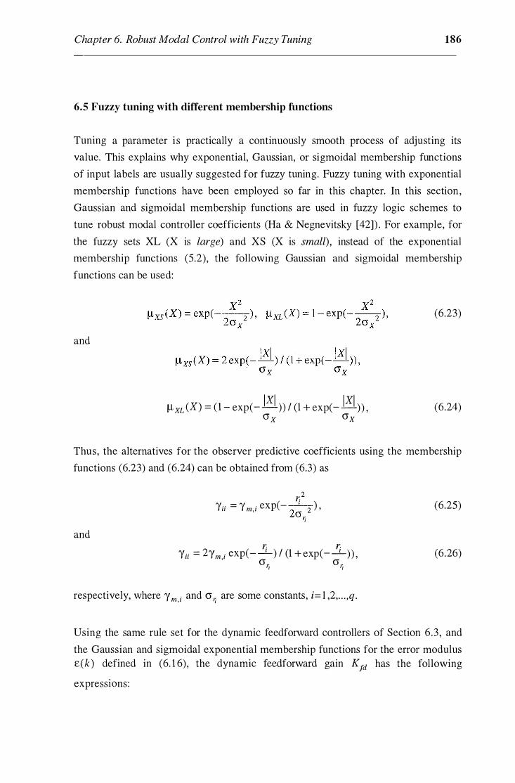
Chapter 6. Robust Modal Control with Fuzzy Tuning 186
6.5 Fuzzy tuning with different membership functions
Tuning a parameter is practically a continuously smooth process of adjusting its
value. This explains why exponential, Gaussian, or sigmoidal membership functions
of input labels are usually suggested for fuzzy tuning. Fuzzy tuning with exponential
membership functions have been employed so far in this chapter. In this section ,
Gaussian and sigmoidal membership functions are used in fuzzy logic schemes to
tune robust modal controller coefficients (Ha & Negnevitsky [42]) . For example, for
the fuzzy sets XL (X is large) and XS (X is small) , instead of the exponential
membership functions (5.2), the following Gaussian and sigmoidal membership
functions can be used:
(6.23)
and
�xL (X) = ( 1 - exp(-E]_)) I (1 + exp(-E]_)) , ax ax (6.24)
Thus, the alternatives for the observer predictive coefficients using the membership
functions (6.23) and (6.24) can be obtained from (6.3) as
and
1:2 'Yu = 'Y m, i exp(-
2� 2 ) ' r;
1: r: "{ ii = 2 "{ m i exp(- -1 ) I (1 + exp(- -1 ) ) , ,
(Jn (Jn 1 1
respectively, where "{ m i and cr n are some constants, i= l ,2, . . . ,q . , 1
(6.25)
(6.26)
Using the same rule set for the dynamic feedforward controllers of Section 6 .3 , and
the Gaussian and sigmoidal exponential membership functions for the error modulus E(k) defined in (6. 1 6), the dynamic feedforward gain Kfd has the following
expressiOns :
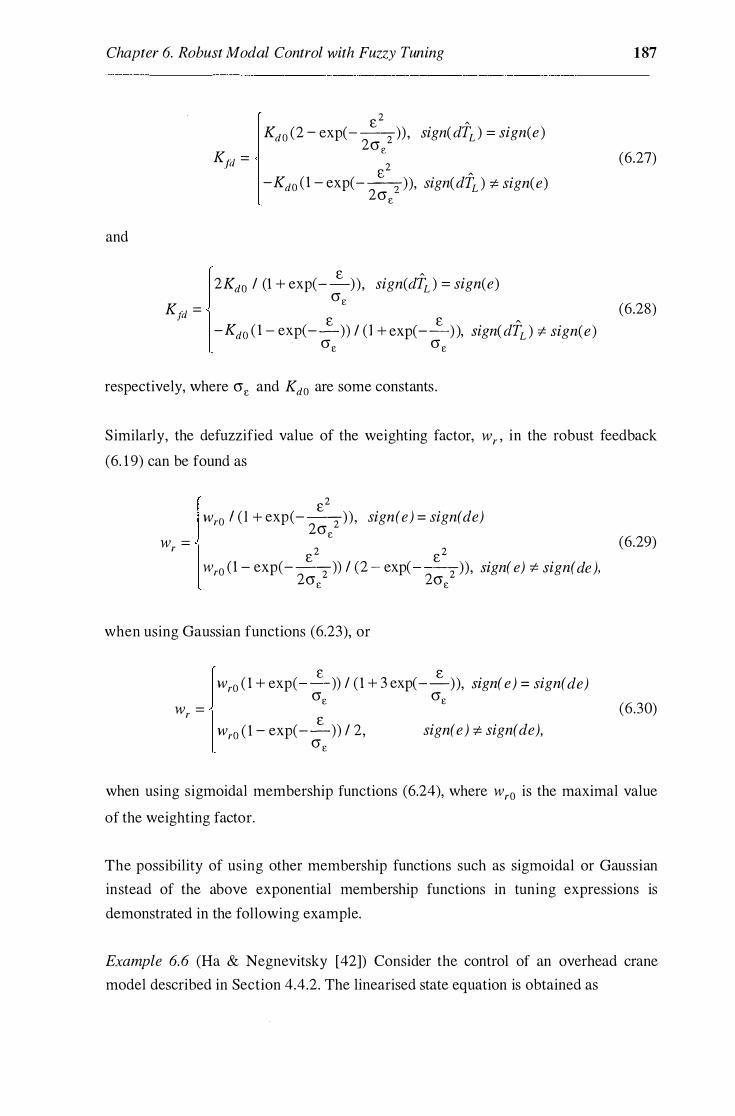
Chapter 6. Robust Modal Control with Fuzzy Tuning
and
K.fd =
Ktd =
£2 A
Kdo (2 - exp(- --2 ) ) , sign( dTL ) = sign( e ) 2cr10
2 -Kdo (1 - exp(-�) ), sign( dTL ) :f:. sign( e)
2crr
£ A
2Kdo I (1 + exp( - -)), sign(dTL ) = sign( e) (')£
£ £ A
-Kdo ( 1 - exp(- -)) I ( 1 + exp(- -) ), sign( dTL ) :f:. sign( e) (')£ (') £
respectively, where crr and Kdo are some constants .
187
(6.27)
(6.28)
Similarly, the defuzzified value of the weighting factor, w r , in the robust feedback
(6. 1 9) can be found as
w = r
£2 Wro l ( l + exp(- --2 )) , sign(e) = sign(de)
2crr
£2
£2
wro (1 - exp( - --2 )) I (2 - exp( - --2 )), sign( e) :f:. sign( de), 2crr 2crr
when using Gaussian functions (6.23), or
w = r
Wro ( 1 + exp(- _£ )) I ( 1 + 3 exp( _ __£ )), sign( e) = sign( de) (')£ (')£ £
Wro ( 1 - exp( - -)) I 2, (') £
sign( e) :f:. sign( de),
(6.29)
(6.30)
when using sigmoidal membership functions (6.24), where wro is the maximal value
of the weighting factor.
The possibility of using other membership functions such as sigmoidal or Gaussian
instead of the above exponential membership functions in tuning expressions is
demonstrated in the following example.
Example 6.6 (Ha & Negnevitsky [42]) Consider the control of an overhead crane
model described in Section 4.4.2. The linearised state equation is obtained as

Chapter 6. Robust Modal Control with Fuzzy Tuning 188
XI 0 1 0 0 XI 0 0
x2 0 - 0. 1625 9. 8 1m 0 x2 0. 985 - 50 = + u + TL x3 0 0 0 x3 0 0
x4 0 - 0. 1625 / l - 9. 8 1( l + m) l l 0 x4 -0. 985 I l -50 I l
where x1 is the trolley position, x2 = x1 , x3 is the swing angle, u is the control voltage
applied to the servo motor, and TL is the unknown load torque due to any
nonlinearities or external disturbances; m is the load mass, and l is the rope length.
The sampling period is chosen as T=0.02 sec. The robust modal controller is designed
at m = m0 = 0.25kg and l = 10= 0.4m.
The closed-loop poles are assigned by the ITAE criteria. The feedback gain in (4) is
calculated by Ackermann's formula kT=(43 .0 1 9 .5 - 1 5 . 1 3 .2) . Choosing
L = (1 0 0 0) , the predictive observer is designed to estimate the unknown input TL
using the measured reading of the trolley position. The static feedforward gain is determined as in (6. 1 1 ), K1s= 50.8 . Since the motor electromagnetic and power
amplifier time-constants are negligible, the dynamic compensation is not necessary (K1d =0). Choosing Q = 14 the robust feedback gain, defined in (6. 1 8) is found to be
k;.=(-43 . - 1 5 .6 27. 1 -21 .6) . The exponential, Gaussian, and sigmoidal membership
functions are used for fuzzy tuning. Table 6.9 gives the values of tuner parameters, 'Ym=0.5, O'r= l , wro= 0.2, and 0'10 =0.2, when tuning with different membership
functions.
Membership function 'Ym (Jr Wro (j' f
exponential 0.5 1 0.2 0.2
Gaussian 0.5 0. 1 0.2 0.07
sigmoidal 0.5 0.5 0.2 0.2
Table 6. 1 9. Tuner parameters
The trapezoidal law is applied for the optimal speed reference of the trolley motion.
Figure 6.2 1 shows the reference (dotted lines) and actual (solid lines) responses of the
trolley position (a) and swing angle (b) with a conventional pole-placement controller. With m = 2m0 , l = 0 . 5l0 and TL=O oscillations due to parameter sensitivity are
observed.

Chapter 6. Robust Modal Control with Fuzzy Tuning
0 . 7.-----�----�----�----�----�
0 . 6
0.5 -
E c: 0 .4
g -� 0 . 3 0..
0 .2
0 . 1
0 �----�----�-----�----�----�
0 . 4
0.3
� 0.2
� 0 . 1 c ClS Cl) 0 c "ji (/) - 0 . 1
-0.2
0
-0.3 0
�
1 00 200 300 ti m e . x 0 . 02sec
(a)
400
�
� A A A A A A v v v v v v v v
1 00 200 300 400 ti m e . x 0 . 02sec
(b)
5 00
5 00
189
Figure 6.2 1 . Position (a) and swing (b) responses with pole placement controller,
m = 2m0 , l = 0. 5 10 , TL=O.
These responses with a fuzzy logic controller (Negnevitsky, Ha et al. [ 1 34]) are
shown in Figure 6.22. While fuzzy logic controller is robust to parameter variations,
its performance is affected by an external load torque, TL. Figure 6.23 depicts the
responses with the proposed controller under the same conditions and
TL = 0. 5Tnom (1 + sin t ) , where Tnom= 0.037Nm. It is observed that the responses in
Figure 6.23 are more robust to both parameter variations and disturbances . Note that
fuzzy tuning with sigmoidal or Gaussian membership functions also provides similar
results.

Chapter 6. Robust Modal Control with Fuzzy Tuning
0 � n) Ol c 1:\"l Ol c §;; (J)
0.7.-----�----�------�----�-----.
0 . 6
0 . 5
E c: 0 .4 0 ·.;::; "i� 0.3 a.
0 .2
0 . 1
o �·'�--·--�----�----�----�------
o 5 0 1 00 1 5 0 200 25 0 tim e . x 0 . 04sec
(a)
0 . 05
0
- 0 . 05 '------'-------'----'---�-----'-------l 0 5 0 1 00 1 5 0 200 25 0
tim e . x 0 . 04sec
(b)
Figure 6.22. Position (a) and swing (b) responses with fuzzy logic controller, m = 2m0 , l = 0. 5/0 , TL=O.
190
The application of fuzzy logic in tuning the coefficients of a robust modal controller
has been verified through the control of an overhead crane model. The fuzzy schemes
adopt human experience for continuously changing the coefficients of a robust modal
controller. Exponential, Gaussian, and sigmoidal membership functions can be
employed to input labels to result in explicit expressions for tuning. It is observed that
robust modal control with fuzzy tuning can result in strong robustness of the system
against parameter variations and external disturbances.

Chapter 6. Robust Modal Control with Fuzzy Tuning 191
0.8
0 . 6
�- 0.4 c: 0 :;::; '(I) g_ 0.2
0
-0.2 _____.__ __
0 1 00 200 300 400 5 00 tim e . x 0 . 02s ec
(a)
0 . 04
0 . 02
0 � af a, c: <\l
g .o.02 � U)
-0.04
-0.06 0 1 00 200 300 400 5 00
tim e . x 0 . 02s ec
(b)
Figure 6.23 . Position (a) and swing (b) responses with fuzzy tuned robust modal controller, m = 2m0 , 1 = 0. 510 , 1� = 0 . 5Tnom (l + sin t) .
6.6 Summary
This chapter has presented a methodology using fuzzy logic and some engineering
heuristics to tune the parameters of robust modal controllers for improving
robustness . Simple tuning schemes are applied for continuously changing the
predictive observer coefficients, the feedforward controller coefficients, and the
robust feedback coefficients.
The predictive coefficients of an unknown input observer are tuned taking into
account the change of estimated disturbances. As illustrated in estimating the load
torque of a two-mass servo system, observer robustness is improved with fuzzy
Chapter 6. Robust Modal Control with Fuzzy Tuning 192
tuning. Conditional schemes are given for tuning the dynamic feedforward coefficient
in relation to the signs of the error and the change of the estimated load torque
disturbance. Robustness achieved by the fuzzy-tuned feedforward compensation is
verified through the control of a robot arm motion, and a two-mass position drive.
Other fuzzy schemes are also proposed to tune the robust feedback gain according to
the signs of the error and the change of error. Simulation results obtained through the
position control of a two-mass resonant system indicate that the observer-based
controllers with fuzzy tuning can be applied to make the system more robust to
parameter and load variations. Thus, it can be feasible in flexible structures where the
problem of vibration suppression and load rejection is challenging.
Using singletons and the centroid technique for defuzzification, all the fuzzy schemes
result in explicit expressions, thus the tuning process is easy and the computational
cost is low. The membership functions for input labels can be exponential as well as
Gaussian or sigmoidal. Servo drives are chosen here as controlled objects, however,
the proposed method can be applied to other linearised dynamic systems suffering
from severe uncertainties.

Chapter 7
Neural Network Application to Motion Control
Artificial neural network for control and systems has developed as an interesting topic
over the last few years, not only in terms of the research being carried out, but also in
terms of the potential range of applications. This chapter provides a brief overview of
recent developments of neural network-based controllers in motion control systems
and some neural network-based approaches to the control of electrical drives and
manipulators with changing parameters and load, and with nonlinearities .
7.1 Introduction
Artificial intelligence (AI), systematically used since the late 1 950's, is a machine
emulation of the human thinking processes . Artificial intelligence tools, such as
expert system, fuzzy logic, and neural network are believed to usher a new area in
motion control in the coming decades (Bose [ 1 1 ]) .
Expert systems, flourishing since 1 960's, are computer programs that emulate the
reasoning process of a human expert in certain domain. The core of the expert system
is the representation of knowledge transferred from human domain expertise.
Knowledge can be shown in two types: the expert knowledge embedded in the
knowledge base, and the data, facts, and statements that are normally embedded in the
database for supporting the expert knowledge. Expert system techniques have the
potential for practical applications in some aspects of power electronics and motion
control. In fault diagnosis and monitoring for AC drives, the expert system can
identify the fault by embedding the expertise of a diagnostic technician. With easily
modified and updated database, the expert system can help in drive product selection.
In real-time expert system-based control, the input parameters are accessed from the
sensors. The expert system is used to process these signals and generate the
appropriate control action. Since its genesis in the mid 1960's , fuzzy logic gradually

Chapter 7. Neural Network Application to Motion Control 194
helped to supplement the expert system and a more general methodology of reasoning
called fuzzy expert system was born. In general, fuzzy expert system which is
applicable wherever the knowledge base of an expert system contains fuzziness , can
provide an enhancement for reasoning with uncertainty and imprecision (Hall and
Kandel [ 166]). Fuzzy logic can be applied to control, diagnostics, modelling, and
estimation. A fuzzy control, as described in Chapters 4, 5, and 6, essentially embeds
the intuition and experience of a human operator, and sometimes those of a designer
and researcher. It can be shown that fuzzy control is basically adaptive in nature, and
can give improved robustness in systems with unknown or ill-defined plant model, or
systems with changing parameters and load. Previous chapters have demonstrated the
use of fuzzy tuning schemes for robustness enhancement in many servo drives. This
chapter deals with the application of another AI branch, artificial neural networks or
neural networks, for this purpose.
The study of artificial neural networks is an attempt to understand the functionality of
the brain. Fundamentally, the human brain forms a massive communication network,
consisting of billions of nerve cells , also known as neurons. These neurons are
interconnected to constitute the biological neural network. The artificial neural
network (ANN) tends to simulate the biological one by electronic computational
circuits. The ANN technology is the most generic for emulating the human thinking
process which is generated by the action of the biological neural network. Gradually
evolving since 1950's , the ANN technology has practically captivated the attention of
scientific community since the beginning of 1 990's (Widrow & Lehr [ 15 ]) . Neural
network applications to engineering problems are many and varied (process control,
diagnostics, identification, pattern recognition, robot vision, flight scheduling, and so
on) . Neural networks can be used for various control and signal processing
applications in power electronics and drives. A neural net can be trained for
diagnostics of a power electronics and drive system. A nonlinear dynamical system,
e.g. in robotics , can be emulated by time-delayed input and output signals with a
feedforward network used in identification and control (Narenda & Parthasarathy
[27]) . In control systems, the use of neural networks is getting increased attention
because of many advantages in speed of adaptation, noise rejection, and tracking
performance over adaptive control techniques (Kraft & Campagna [ 167]) . The
following sections are involved in a brief review on neural network-based control
(Hunt et al. [ 1 68]) and details on some of its applications in servo systems and
systems with severe nonlinearity and parameter variation problems (Ha & Negnevitsky [34, 44] , Ha [45] , Palis, Ha et al. [33 , 165]) .
Chapter 7. Neural Network Application to Motion Control 195
7.2 Neural networks: basic concepts and application to control
In recent years there has been an increasing interest in studying the mechanisms and
structure of the brain. The human brain is said to have around 100 billions neurons or
nerve cells, each neuron is interconnected to 1 000 to 10 000 other neurons. A
biological neuron is a processing element that receives incoming impulses via input
paths called dendrites. If the number of incoming impulses within a certain period of
time exceeds some thr�shold, the neuron will "fire," producing an output impulse
along the axon that connects to dendrites of many other neurons. When a neuron fires,
it transmits its impulse via the axon and synapses. Each synapse is an infinitesimal r : .. gap in the dendrite which is filled with neurotransmitter fluid that either accelerates or
retards the flow of electrical charges. These electrical signals go to the nucleus or
soma of the neurons. The adjustment of the impedance or conductance of the synaptic
gap leads to "memory" or " learning process" of the brain (Bose [ 1 1 ]) .
7.2. 1 Neural network architecture
The artificial neuron (so-called neuron, node, cell, connectionist model, perceptron, or
adeline) is a processing element having the standard and unifying architecture shown
in Figure 7. 1 (Hunt et al. [ 1 68]) . The basic model of a neuron constitutes of three
components: a weighted summer, a linear dynamic system, and a nonlinear function.
The weighted sum is described by
N M vJt) = :L ai1y1 (t) + L hikuk (t) + wi ,
J=! k=1 (7. 1 )
where y1 , j = l , . . . , N, are the neuron outputs; uk , k = I, . . . , M , are the external inputs;
and au , hu( , and wi are the corresponding weights. The weights are connection
strengths whose function are analogous to that of synaptic junctions in a biological
neuron. The weights can be positive or negative corresponding to acceleration or inhibition of the flow of electric signals . The transfer function H(s) = � (s)/Xi (s) for
the linear dynamic system have the following common forms:
(7 .2)

Chapter 7. Neural Network Application to Motion Control 196
y l
U l (;:_� �,-�
vi [� Xi K�l yi )
Linear Nonlinear
. Dynamics Function
�, __ ___)
Figure 7 . 1 . Architecture of an artificial neuron.
where a0 , a 1 are constants . The non-dynamic nonlinear function Yi = g(xi ) can be
classified as differentiable or non-differentiable, pulse like or step like, and positive
(bound to the range (0, 1 )) or zero mean (bound to the range (- 1 , 1 )) . Some standard
functions are threshold, signum, sigmoid, Gaussian, and hyperpolic tangent,
respectively:
g(x) = +l if x > O else O, g(x) = +1 if x > O else - 1,
I 2/ 2 g(x) = 1 (1 + e-x ) , g(x) = e-x cr ,
and g(x) = tanh(x) = (ex - e-x )/(ex + e-x ) .
(7 .3)
The sigmoid is positive, monotonic, differential, and step-like having the largest
incremental gain at zero signal. Thanks to these particularly interesting properties, it is
most commonly used i n neuron models .
The three components of the neuron shown in Figure 7 . 1 can be combined in various
ways. The behaviour of networks resulting from such a combination depends on the connection matrix A = (ai) NxN and on the form of H(s) . The interconnection of
neurons allows us to encode relations between the variables giving different powerful
processing capabilities . Neural networks can generally be classified as feedforward or

Chapter 7. Neural Network Application to Motion Control 197
feedback types. In multilayer feedforward networks, the connection of several layers
gives the possibility of complicated nonlinear mapping between the inputs and the
outputs. This capability can be used to implement classifiers or to represent complex
nonlinear relations among the variables. Such networks are typically static, that i s
H(s) = 1. The connection matrix A i s such that the outputs are partitioned into layers
so that a neuron in one layer receives as inputs only from neuron outputs in the
previous layer (or only from the network inputs in case of the first layer) as shown in
Figure 7.2.
NN- 1 NN-2
Figure 7 .2. Multi-layer feedforward networks
Dynamic or recurrent networks are qualitatively different from static ones, because
their structure incorporates feedback. The introduction of feedback produces a
dynamic network with several stable points. The general equation can be expressed as
x(t) = F(x(t), u(t), 8), y(t) = G(x(t), 8),
(7 .4)
where x(t) is the vector of the state variables, u(t) the external inputs, y(t) the
outputs, 8 the parameters of the network, F is a function that represents the network (''
fe¢(iback structure, and G represents the nonlinear relation between the state
variables and the outputs. In Kohonen [ 169] , feedback networks were introduced in
the context of associative memory (CAM) problems for pattern recognition. There
exist numerous neural network architectures, however, at present, the majority of
power electronics and motion control applications use the feedforward architecture
(H(s) = 1) with backpropagation algorithm (Bose [ 1 1 ]) . Figure 7.3 shows a typical
feedforward network with three inputs and two outputs, having three layers: input
layer /, hidden layer J, and output layer K. The number of hidden layers and the
number of neurons in each hidden layer (four in Figure 7.3) depend on the design
considerations .

Chapter 7. Neural Network Application to Motion Control
X l
INPUT -� X2
INPUT LAYER
X3 SCALE FACTOR
HIDDEN LAYER
:> Y l
OUTPUT
V4 ACTUAL OUTPUT PATTERN
WEIGHT DESIRED ADJUSTMENT 1<-E--1 OUTPUT ALGORITHM PATTERN
ERROR
Figure 7 .3 . A three-layer feedforward network
7.2 .2 Learning in neural networks
198
The application of artificial neural networks normally proceeds in two phases: the
recall phase and the training phase. In the recall phase, the networks, which have been
trained with appropriate data with constant coefficients, provide a fixed behaviour
with constant coefficients in their architecture as described above. The training phase
presents algorithms for automatic adjustment of network coefficients, a process called
learning. A learning algorithm, associated with any change in memory as represented
by the weights, is a parametric adaptation algorithm. If an input set of data
corresponds to a definite signal pattern, the network can be trained to give a
correspondingly a desired pattern at the output. the capability of learning is explained
by the distributed intelligence contributed by the weights. The input-output pattern
matching is possible if proper weights are selected. The supervised learning process
incorporates an external reference signal (learning by a teacher) or global information
about the system. The unsupervised learning process incorporates no external
reference signal and relies only on local information and internal signals (learning
with a critic) . In supervised learning, the actual output pattern can be compared with

Chapter 7. Neural Network Application to Motion Control 199
the desired output pattern and the weights can be adjusted by an algorithm until the
pattern matching occurs . At the end of training when the error is adequately small, the
network can recall all the trained output patterns (look-up table function), and
interpolate and extrapolate the trained patterns as well.
In multi-layer non-dynamic networks, backpropagation algorithm is commonly used. In the beginning, the network is assigned random weights ( wiJ and wik in Figure 7.3) .
For a given input-signal pattern, the output pattern is calculated step-by-step in the
forward direction. A cost function given by the squared error between the net output
for the set of input patterns is generated and this is minimised by gradient descent
method adjusting the weights one at a time. The net input to the j th neuron (node) in
layer J (hidden layer) is :
M net1 = L wiJoi ,
i=l (7 .5)
where j is the processing unit under consideration, oi is the output of the i th neuron
connected to the j th neuron, wiJ is the connection weight between the i th and j th
neurons, and M is the number of neurons feeding the j th neuron ( M =3 in Figure
7.3) . The output of the .f th node is:
(7 .6)
where g is the nonlinear activation function, usually a sigmoid:
(7.7)
where the net parameter 81 serves as a threshold or bias and the effect of 80 is to
modify the sigmoid shape (Figure 7.4). Similarly, for the input and output of the k th
node in layer K are:
N netk = L w1kv1 ,
J=l Yk = g(netk ),
(7 .8)
respectively, where N is the number of neurons in the hidden layer ( N =4 in Figure
7 .3).

Chapter 7. Neural Network Application to Motion Control
1 .0
K-- e· -� .J netj
Figure 7 .4. Sigmoid with bias and shape modification.
200
In the learning phase, the p th pattern is presented as input (p = 1, 2, . . , P) , and the
weights in all connecting links together with the thresholds are adjusted such that the
target or desired output tf is obtained at the k th output node (k = 1, 2, . . , S ) . Once this
adjustment has been accomplished by the net, another pair of patterns and targets is
presented, and the net is asked to learn that association also. Ideally, the net will find a
single set of weights and biases that will satisfy all the (pattern, target) pairs presented
to it. However, the outputs yf and the desired values tf are generally not the same.
For the pth input pattern, the square of the error for all the output-layer neurons is
given by
Ep = ± ce - yPl (tP - yP ) = ± ctf - yf )2 . k=l The average system error for the set of P patterns is written as
1 p s E = - 2. 2- Ctf - yf )2 . 2P p=l k=I
(7 .9)
(7 . 10)
The weights are changed to reduce the cost functional to a minimum value as rapidly
as possible by the gradient steepest-descent algorithm. Starting from the output layer,
the gradient method leads to the update equation:
(7 . 1 1 )
where w Jk ( n + 1) is the new weight, w Jk ( n ) is the old weight, 11 >0 is the learning rate,
and �wJk (n) is the weight incremental change. The partial derivative aEPjaw1k can
be evaluated using the chain rule:

Chapter 7. Neural Network Application to Motion Control
aEP _ aEP anetk _ aEP -- - ---- - -- vi . awjk anetk awjk anetk
By defining
we obtain the delta rule of the weight change for any k th output-layer neuron:
Applying the chain rule to 8k yields
O _ _ aEP _ _
aEP ay{ k - anetk
-ay{ anetk
= (tf - yJ: )g� (netk )
201
(7 . 1 2)
where the pth subscript denotes the pattern number. Using sigmoid of the form (7.7)
a p
for the nonlinear activation function, we have a
Ykt
= g� (net" ) = yf (1 - y{ ) , thus ne k
the delta 8k in (7 . 1 2) i s given by the following expression:
(7. 13)
If the weights do not link with the output neurons directly, the update equation is
written as
aEP w . . (n + 1) = w .. (n) - ,., = w . . (n) + D.w . . (n) lj 1] • • a c ) lj lj , wu n
where the incremental change D.wiJ for hidden layer units is calculated by
or
(7. 14)

Chapter 7. Neural Network Application to Motion Control 202
(7 . 1 5)
The factor CJEP jCJv 1 can be rewritten for its evaluation in terms of known quantities
(Pao [ 170]) :
In this case, since
81 = gj (net1 )I,8kwik ' k
when using sigmoid (7 . 7) for the nonlinear activation function, the expression for the delta 81 in (7 . 15) can be obtained as
81 = v) ( l - v) ) I, 8kwJk . (7 . 1 6) k
The iterative process propagates the error backward in the network (backpropagation)
following (7 . 12) , (7 . 1 3 ) and (7 . 1 5) , (7. 1 6) is called the learning procedure with the
generalised delta rule formulated by Rumelhart, Hinton, and Williams [ 1 7 1 ] . Note that the thresholds 81 are learned in the same manner as the weights. The weights are
iteratively updated for all the P training patterns. In a successful learning exercise, the
system error will decrease with the number of iterations, and the procedure will
converge to a stable set of weights. The choice of a large value for the learning rate 11 leads to rapid learning but might also result in oscillations. To avoid local error minima, a momentum term a[wi/n) - wu (n - 1)] is added to the right of (7. 14), thus
the weight change at the (n + 1)th step is given by
(7 . 1 7)
where a is a proportional constant. A finite momentum constant a tends to dampen
oscillations but can also serve to slow the rate of learning. The speed of
backpropagation can be increased by the use of adaptive learning rate which attempts
to keep 11 as large as possible while keeping learning stable:
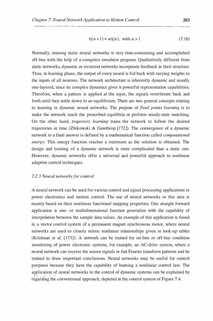
Chapter 7. Neural Network Application to Motion Control 203
11(n + l ) = u'll(n) , with u > l (7 . 1 8)
Normally, training static neural networks is very time-consuming and accomplished
off-line with the help of a computer simulator program. Qualitatively different from
static networks, dynamic or recurrent networks incorporate feedback in their structure.
Thus, in learning phase, the output of every neural is fed back with varying weights to
the inputs of all neurons . The network architecture is inherently dynamic and usually
one-layered, since its complex dynamics gives it powerful representation capabilities.
Therefore, when a pattern is applied at the input, the signals reverberate back and
forth until they settle down to an equilibrium. There are two general concepts relating
to learning in dynamic neural networks. The purpose of fixed points learning is to
make the network reach the prescribed equilibria or perform steady-state matching.
On the other hand, trajectory learning trains the network to follow the desired
trajectories in time (Zbikowski & Gawthrop [ 172]). The convergence of a dynamic
network to a final answer is defined by a mathematical function called computational
energy. This energy function reaches a minimum as the solution is obtained. The
design and training of a dynamic network is more complicated than a static one.
However, dynamic networks offer a universal and powerful approach to nonlinear
adaptive control techniques .
7.2 .3 Neural networks for control
A neural network can be used for various control and signal processing applications in
power electronics and motion control . The use of neural networks in this area is
mainly based on their nonlinear functional mapping properties. One straight forward
application is one- or multidimensional function generation with the capability of
interpolation between the sample data values . An example of this application is found
in a vector control system of a permanent magnet synchronous motor, where neural
networks are used to closely mimic nonlinear relationships given in look-up tables
(Krishnan et al. [ 1 73 ] ) . A network can be trained for on-line or off-line condition
monitoring of power electronic systems, for example, an AC-drive system, where a
neural network can receive the sensor signals or fast Fourier transform patterns and be
trained to draw important conclusions. Neural networks may be useful for control
purposes because they have the capability of learning a nonlinear control law. The
applicat,ion of neural networks to the control of dynamic systems can be explained by / .�- r / r
regarding the conventional approach, depicted in the control system of Figure 7 .4.
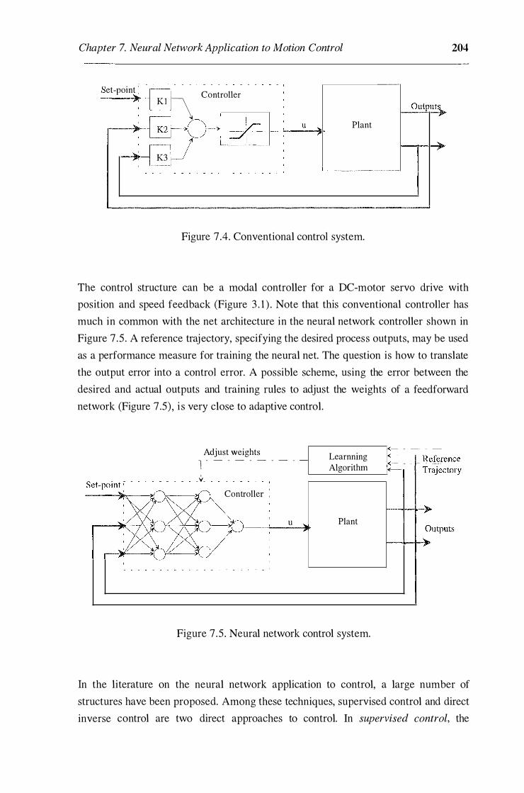
Chapter 7. Neural Network Application to Motion Control 204
---et-point : Controller Kl \ Output�
, "'' Gil--& � u "' Plant ,. ,.
-� �
--
-
---
----""" --""'
,. , K3
'----- -- -
Figure 7 .4. Conventional control system.
The control structure can be a modal controller for a DC-motor servo drive with
position and speed feedback (Figure 3 . 1 ) . Note that this conventional controller has
much in common with the net architecture in the neural network controller shown in
Figure 7 .5 . A reference trajectory, specifying the desired process outputs, may be used
as a performance measure for training the neural net. The question is how to translate
the output error into a control error. A possible scheme, using the error between the
desired and actual outputs and training rules to adjust the weights of a feedforward
network (Figure 7 .5) , i s very close to adaptive control.
Adjust weights -1 - - - - - - - - - Learnning Algorithm '
_y_
Controller :
u Plant __;,_ __ ....
Figure 7.5 . Neural network control system.
In the literature on the neural network application to control, a large number of
structures have been proposed. Among these techniques, supervised control and direct
inverse control are two direct approaches to control. In supervised control, the
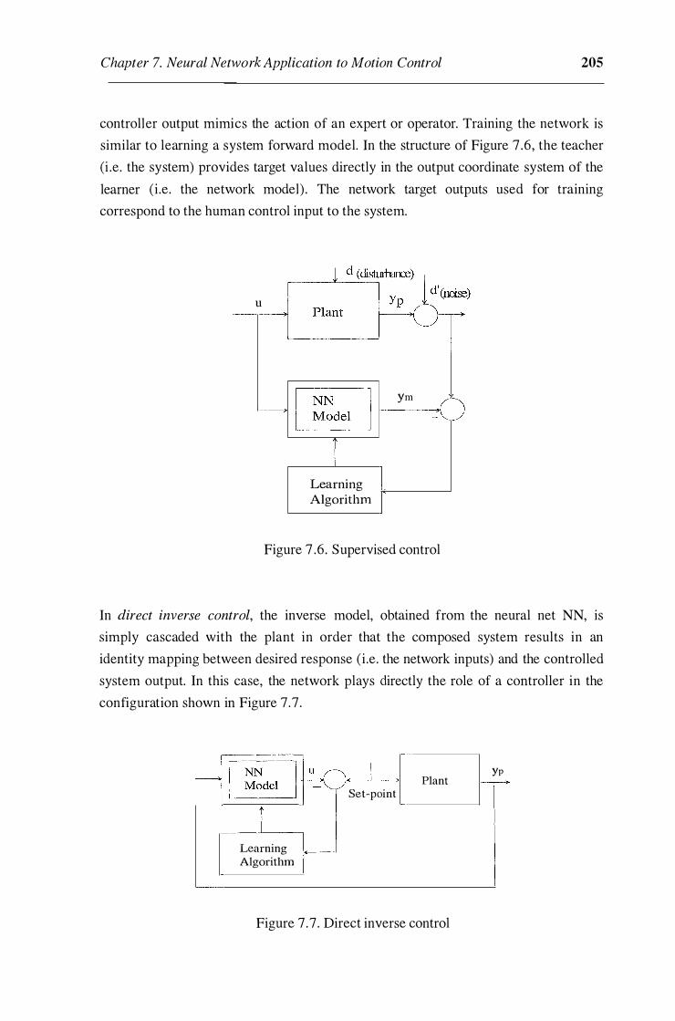
Chapter 7. Neural Network Application to Motion Control 205
controller output mimics the action of an expert or operator. Training the network is
similar to learning a system forward model. In the structure of Figure 7 .6 , the teacher
(i .e. the system) provides target values directly in the output coordinate system of the
learner (i.e. the network model) . The network target outputs used for training
correspond to the human control input to the system.
u --,--*
IT�J ym
� --1
I Learning Algorithm
Figure 7 .6. Supervised control
In direct inverse control, the inverse model, obtained from the neural net NN, is
simply cascaded with the plant in order that the composed system results in an
identity mapping between desired response (i.e. the network inputs) and the controlled
system output. In this case, the network plays directly the role of a controller in the
configuration shown in Figure 7.7 .
INN! u
�:_j
Learning Algorithm
Plant Set-point
Figure 7.7 . Direct inverse control
YP

Chapter 7. Neural Network Application to Motion Control 206
The other control structures using neural networks combined with a stable reference
model (model reference control) or with a system model (internal model control) are
outlined in Hunt et al. [ 1 68] . While recurrent networks are universal, parametric
systems that can be used as identifiers and dynamic controllers, the complexity of
their analysis and design is a challenging problem. At present, most of neural
network-based applications in power electronics and drives exploit static networks
possessing proven capabilities of arbitrary nonlinear approximation.
7.3 Neural network implementation of a fuzzy logic controller
As stated in the section above, a neural network can closely approximate any control
relationship of practical interest, to learn such a relationship through a training
process, and also to interpolate the controller outputs the inputs do not belong to the
training set of the inputs. Essentially, a neural network controller is a nonlinear
parametric system which can be easily worked out because of its mathematical rather
than linguistic nature of a fuzzy logic controller. A straightforward approach is to
implement a fuzzy logic controller in a neural network and expect the system
performance with neural control will be as good as with fuzzy control . This approach
is motivated by the work described in Buja & Todesco [ 174] . In this section, it i s
i ll ustrated through the control of a laboratory crane model. The plant dynamics and
the design of a fuzzy logic controller was described in Section 4.4.2.
7.3. 1 . General system description
A common task for motion control of a swinging load, e.g. in crane, pendulum, and
cart-pole systems, is to move a load from an initial position to a specified final one.
The loads are usually varying. The inertial parameters of the crane are also uncertain .
On the other hand, when a load is transported by a crane, i t often exhibits oscillatory
swings. The back and forth swinging of the load during the transfer motion can cause
considerable problems, especially in bounded places, and in the presence of
uncertainties in the system dynamics. Conventional techniques can be applied to
address this subject, for example, optimal control in Yoshida & Kawabe [ 1 7 5 ] ,
adaptive control i n Soussi & Koivo [ 176] , and robust modal control as described in
Chapter 3 . Fuzzy logic has recently arisen as an attractive tool to control ill-defined or
parameter-variant plants. A fuzzy logic controller (Negnevitsky, Ha et al. [ 1 34]) or a
robust modal controller with fuzzy tuning (Ha & Negnevitsky [42]) can be used for
positioning a swinging load. However, fuzzy logic controllers usually suffer from a

Chapter 7. Neural Network Application to Motion Control 207
heavy computation burden when implemented. Moreover, its performance relies on
the soundness of know ledge acquisition techniques and the availability of human
experts . In the following a neural network controller is used to implement the fuzzy
logic controller described in Section 4.4.2 for positioning the load of an overhead
crane model. The validity of the proposed methods are verified through simulation
and experimental results .
The plant block diagram i s shown in Figure 7.8 (Ha & Negnevitsky [34]) where
analog/digital (AID) and digital/analog (D/A) converters are used at the interface (see
Section 4.4.2). The neural network (NN), shown in Figure 7 .9, has two inputs e and
8 , a hidden layer, and an output u of one linear neuron, where e is the trolley
position error, 8 is the chain angle, and u is the control signal.
X ref I I I I I I I
Figure 7.8 . Block diagram of the control system.
e ,
q ,
Figure 7.9. Network schematic diagram

Chapter 7. Neural Network Application to Motion Control 208
In order to obtain a good approximation and to reduce the training time, radial basis
function networks (see, e.g. , Chen et al. [ 177]) are chosen in the hidden layer. Radial
basis networks are non-dynamic networks with a better approximation property in
comparison with the other feedforward networks. An approximation scheme is said to
have the property of best approximation if in the set of approximating functions there
is one which has minimum distance from the given function (Poggio & Girosi [ 1 78]) .
The structure of a radial basis neuron with N inputs is shown in Figure 7 . 1 0. Its output is a Gaussian function of the Euclidean distance between the input vector P; and its weight vector (the centre of the basis function) w; , multiplied by the bias h; :
(7 . 1 9)
Pil
Pij -G---
y · 1,_
p�-
1� Figure 7. 1 0. Radial basis neuron.
The bias h; , which is the inverse of the radial arm or spread constant cr; (b; = ljcr; ),
allows the sensitivity of the radial basis to be adjusted. As with the sigmoidal
feedforward networks, the number of neurons depends on the size of the training data.
and the choice of the basis function centres. Radial basis networks may require more
neurons than feedforward backpropagation networks, but they can be trained in a
fraction of the time it takes to train standard static networks.
7. 3.2. Simulation and experimental results
For implementing the non-linear relationship u = G(e, 8) obtained from the fuzzy
logic controller inputs and output (see Section 4.4.2), the neural network undergoes a
supervised two-stage training (Ha & Negnevitsky [34]) . In the first stage, the neural

Chapter 7. Neural Network Application to Motion Control 209
net learns the desired input-output relationship in the transient process . A pattern of
500 two-element input vectors and a target of the associated one-element output
vector are used for training. The net error goal is set at 10-4 in the transient stage and
10-Jo in the steady-state stage. The maximal number of neurons in the hidden layer
depends on the appropriatd choice of the radial basis function spread constant to avoid
underlapping and overlapping. Table 7 . 1 summarises the network parameters obtained
to achieve the given error goal. Figure 7 . 1 1 depicts the sum-squared network error in
two training stages.
Process
Transient
Steady-state
-1 1 0 g w -2 -g 1 0 :u :::1 CJ' -3 l{l 1 0 E :::1 (f) -4 1 0
-5
Spread constant Error goal No. neurons in the hidden layer
w-3 w-4 1 10
w-6 1 0-10 287
Table 7 . 1 . Network parameters.
0 -6 1 0
JJ 1 o-s ijl ...... -10 � 10 · - - - - - - - · - - - - - - - · - - · · - - - - - - - - - - - -- - - - - - - - - - - - - - - - - - --
CJ' "? -12 E 1 0 :::1 (f)
1 0 ·14
1 0 '----�--'---�---'-----' 0 20 40 60 80 1 00 0 50 1 00 1 50 200 250 E oach E oach
(a) (b)
Figure 7. 1 1 . The sum-squared in (a) the transient stage, and (b) the steady-state stage.
The simulated swing and position responses with a step input reference are shown in
Figure 7 . 1 3 and Figure 7 . 14, respectively, where the dot-dashed line represents the
response obtained from a fuzzy logic controller and the solid line from its neural net
implementation.

Chapter 7. Neural Network Application to Motion Control 210
ti m e . rx 3 msec\
Figure 7. 1 3 . Swing responses with fuzzy and neural controllers.
0. 1 2 .....----.,.-----------,----......,
0.08
0.06
1 000 2000 3000 4000
Figure 7 . 14 . Position responses with fuzzy and neural controllers .
Figure 7 . 1 5 plots the experimental swing responses obtained from the proposed neural
network implementation of the fuzzy logic controller described in Section 4.4.2, and
from conventional P and PI controllers. These response practically coincide with those
shown in Figure 4.27 . The results demonstrate that a neural network can learn the
fuzzy logic controller input-output relationship to achieve practically the same control
performance as obtained from fuzzy control.

Chapter 7. Neural Network Application to Motion Control
00 �-----------------------------� -� 40 ,' ,"', ,·\ ' · .. , ' � 2) IJ I J ' \ / t , \ I ' 01 ' I'\ ; : , ""\. · ', r- .' ',1�\ : • ,., ; Y"' · · - · · · · Proi'Yirtional � 0 ' ' � �· ,· :-- ' . ;.' \ \ I"� .... '""."""' "1 p .. I :.. I I ' \ / \' (Kp=2) .._, <P'. >� ', <ef'J "t ;'t{ : � '"" cq ;� ', -:J:; _.. �� /cp � -20 .. ' 0 ' rr 0J ' (Y) ' • "¢ ' L() ,«::1 �'-- • '
n (Kp==2·K'i-10� ·;; ' t � J , t ' ' ' , • .. , ...... ...... - rl ' - � rn -40 - " - � � "' -- NN -00�--�--------------------�--� L-----------�
Time(s) Figure 7 . 1 5 . Experimental swing responses
7.4 Neural network-based controller for tracking systems
211
Tracking a given trajectory is a common task in industrial drives. As noted in Dote
[65] modern control techniques such as the sliding mode, adaptive controls, robust
control can be successfully applied to obtain high quality tracking performance.
However, the effectiveness of these techniques diminishes when the servo drives are
excessively affected by structured and/or unstructured uncertainties. Even in a well
structured setting for an industrial use, some electromechanical objects, such as
robotic manipulators, are subject to structured and/or unstructured uncertainties.
Structured uncertainty originates from the imprecision of the system description,
parameter variations, and unknown load torques. Unstructured uncertainty is
characterised by the unmodelled dynamics resulting from the presence of high
frequency mode, time-delays, and severe nonlinearities. For improving robustness,
several control techniques are evolving such as the sliding mode in variable structure
systems (Utkin[7] , DeCarlo et al. [70]) , self-tuning and model reference adaptive
controls (Astrom [69] , Egami et al. [ 102]) . Sliding mode control is efficient dealing
with structured uncertainty such as changing parameters and load. However, the
observation noise and the chattering phenomena due to large control gains are
challenging issues and there is a trade-off between robustness and chattering.
Moreover, sliding mode control requires a valid model and/or dynamics of the
controlled object. Thus, the controller is, mainly due to the structured uncertainty,
sensitive to large parameter variation and noise. Conventional adaptive control
schemes require information about the plant structure and may not guarantee the
system stability in the presence of unmodelled dynamics. In addition, adaptive control
algorithms are usually complicated and thus , need excessive computation effort for
real-time implementation. Although the adaptive controls are effective in

Chapter 7. Neural Network Application to Motion Control 212
csnnpensating the influence of the structured uncertainty' it is not clear that adaptive
means can overcome the unstructured uncertainty.
Recently, there has been increasing interest in designing and implementing an
intelligent controller which can adopt skills of an experienced operator. Artificial
intelligent tools such as expert system, fuzzy logic, and neural network have advanced
significantly in recent years and are believed to find wide applications in industrial
electronics and motion control (Bose [ 1 1 ]) . Fuzzy logic controllers (Lee [ 1 1 0]) , which
are capable of providing an effective solution to most complex systems, can be
designed with a minimum understanding of the controlled object. Fuzzy tuning has
been demonstrated to be a rigorous tool to deal with uncertainties in servo drives (Ha
[ 148] , Ha & Negnevitsky [37]) . However, fuzzy logic controllers may suffer from a
heavy computational burden required to translate the fuzzy inference into a control
action. As mentioned in Section 7.2, artificial neural networks, which have the ability
to mimic the adaptive distributed architecture in the human brain, provide potential
alternatives to tackle the problem mentioned above. The error backpropagation
algorithm (Werbos [25]) is widely used to train neural networks. Most of the neural
networks applied to servomechanism learn the inverse dynamics of the controlled
object (Lee et al. [32] , Saad et al. [ 1 79]), based on an observation of its inputs and
outputs. In practice, training neural networks in some cases may take time in order to
achieve the error goal, and thus, make on-line training infeasible. For trajectory
tracking control, neural networks can also be applied to generate the proper control
action without the necessity to identify or learn the plant dynamics. Tai et al. [ 1 80]
proposed a neural network used as an classifier to recognise the patterns of the error
signal between the plant output signal and the reference signal. An appropriate control
action is calculated proportionally to the control error for each pattern. In fact, a
proportional type controller cannot adequately meet high quality servo requirements .
In fuzzy control systems, proportional-derivative type controllers are usually applied
to increase stability and reduce overshoot (Malki et al. [ 1 59] ) . In this section, the
tracking performance is improved by using the neural network that can be trained to
cluster the groups of both the control error and its derivative which an appropriate
control action would correct. The control signal is generated without a priori
knowledge of the plant dynamics. Thus, it can be implemented in a variety of servo
drive applications. The proposed scheme is verified through the control of an
overhead crane model of the previous section. Simulation results demonstrate the
servo robustness with respect to parameter and load variations, and to nonlinear

Chapter 7. Neural Network Application to Motion Control 213
dynamics (Ha & Negnevitsky [44]) . The application of this approach can be extended
to multi-mass servo systems (Ha [45]) .
7.4. 1 . Network architecture and learning
A three-layer feedforward neural network is utilised with the error backpropagation
learning method. For learning the plant inverse dynamics, a multilayer neural network
with sigmoidal nonlinearities can approximate any arbitrary functions representing the
plant input-output relationship. However, it is believed that in some tracking systems,
identifying or learning the plant dynamics is not necessary as long as a proper control
signal can be generated to make the output closely, quickly, and robustly follow any
prescribed reference signal. In the following, the neural net is used as a pattern
classifier to learn decision functions for patterns of the control error and its derivative,
based on training set examples. The net consists of input, hidden, and output layers as
shown in Figure 7 . 1 6 .
e*
Figure 7 . 16 . Neural network schematic diagram.
The input layer contains R=2 units (nodes or neurons) corresponding to the scaled
modulii of the control error e *
and its time derivative e * . The hidden layer has a
certain number of S units . The value of S will be chosen for an effective training
process to achieve the error goal without overlearning. The output layer consists of
K=4 neurons corresponding to the error patterns p1 (e* is large) , p2 (e" is medium) and p3 (e
* is small), and derivative-of-error pattern v1 (e" is large). The log-
sigmoidal transfer function (7 .7) is used for each neuron. Using the subscripts i, j and

Chapter 7. Neural Network Application to Motion Control 214
k for input, hidden and output layers, respectively, the output of the k-th node (unit, or
neuron) in the output layer is
(7 .20)
where ek serves as a bias (or threshold) of unit k and eo determines the slope of
sigmoid (here 80= 1 ) ,
(7 .21 )
i s the input to the k-th node (k = 1 , 2, 3, 4 ) in the output layer, and wkJ i s the weight
from unitj in the hidden layer to unit k in the output layer.
Similarly, the output of the s-th node in the hidden layer is
(7.22)
where
(7 .23)
is the total inputs to unit j (j = 1 , 2, . . . , S ) in the hidden layer, and w Ji is the weight
from unit r in the input layer to unit s in the hidden layer.
The network is trained by a number of pattern pairs. Each pair consists of an input
pattern and a corresponding desired output pattern. Through the learning process, an
energy function
(7 .24)
which is the mean squared error between the actual outputs opJ and the desired
outputs (target) tPi due to an input pattern P, is minimised by changing the weights
and biases in a gradient descent manner. Using the generalised delta rule for the net
with backpropagation of error, described in Section 7.2, the deltas are given by the
following expressions

Chapter 7. Neural Network Application to Motion Control
81 = o1 ( 1 - o1 )L, o�cw�q , k
215
(7.25)
(7.26)
for the output layer and hidden layer, respectively, where tk is the target. In order to
avoid a shallow local minimum, momentum is added to backpropagation learning by
making weight changes equal to the sum of a fraction of the previous weight change
and the new change suggested by the backpropagation rule (7 . 17):
(7.27)
where 11 is the learning rate, a is the momentum constant, and n is the iteration step
for which a set of input patterns are presented to the net.
7.4.2. Neural-network based controller design
The main idea behind this approach is to classify regwns from input-output
measurements and use them as feedforward rules to generate an appropriate control
signal. Control knowledge confirms that in order to improve robustness not only the
control error but also the change of error should be taken into account. Here, similarly
to a fuzzy logic controller, the control signal is calculated from a look-up table rather
than by self-tuning or model reference approaches. The block diagram of the control
system is shown in Figure 7 . 17 (Ha & Negnevitsky [44]) .
I \ 1 TL Xref el I -' X I NN-based f ' ' -
� Controller f---:1 Plant X Xref ' /
; , -
� �
Figure 7 . 17 . Block diagram of the control system.

Chapter 7. Neural Network Application to Motion Control 216
The neural network-based controller consists of a preprocessing unit, a neural
network classifier, a look-up table, and a servo drive unit. The preprocessing unit recognises the signs of the control error e == x,4 - x and its time derivative
e = .X ref' - .X , scales their values into the range [0, 1 ] , and partitions them into several
groups. The three-layer neural network classifier, as shown in Figure 7. 1 6, has two
inputs, the scaled modulii of the control position error e *
and velocity error e" , and four output neurons corresponding to the patterns p1 , p2 , p3 , and v1 . Assuming that
the values of e * and e * are frequently found in the vicinity of 0, 0.2, 0.475, 0. 85 and 0, 0.65, respectively, the ranges of e * and e* corresponding to the patterns p1 , p2 , p3 ,
and v1 are specified as in Table 7.2.
Group *
and e * ranges Output patterns Control action, ua e
index P1 P2 P3 VI
1 [0.7, 1 ] ; [0.3 , 1 ] 1 0 0 1 kP3sign(e) + kvsign(e)
2 [0.7, 1 ] ; [0. , 0 . 1 ] 1 0 0 0 kP3sign(e)
3 [0.35 , 0 .6] ; [0.3, 1 ] 0 1 0 1 kP2sign(e) + kvsign(e)
4 [0.35 , 0 .6] ; [0., 0. 1 ] 0 1 0 0 kP2sign(e)
5 [0. 1 , 0.3] ; [0. 3 , 1 ] 0 0 1 1 kP1sign(e) + kvsign(e)
6 [0. 1 , 0 .3] ; [0. , 0. 1 ] 0 0 1 0 kP1 sign(e)
7 [0. , 0.05] ; [0 .3 , 1 ] 0 0 0 1 kposign( e) + kvsign( e )
8 [0. , 0 .05] ; [0 . , 0. 1 ] 0 0 0 0 kposign(e)
Table 7 .2. Look-up table for e * and e* ranges, output patterns , and control action.
Within each group, three points are randomly chosen as the training patterns . With
S=30 hidden neurons , the learning rate 11=0. 1 and momentum a= 0.9, the error goal,
which is set equal to 0.0 1 , is reached after 253 10 iteration cycles. The sum-squared
error of the training process is shown in Figure 7. 1 8 .
Figure 7 . 19 describes in details the network structure and the feedforward training
process.

Chapter 7. Neural Network Application to Motion Control 217
en
•
en
Train ing for 2531 o E poc hs ..... �
e 1 o� .-----.------,-----.------.-----� ,_ w
30x2
Figure 7. 1 8 . Sum-squared network error.
..... ........ ........ . . . .......... ........ . ···· : p
l !�
4x30 �� 30 4x30 ! � ----')-! 30xl
3:� L 3:x�4 4x30 } "�[r I p
p23 )
� l v l - ,...� 30 :----+
4xl ... ............... ..... ...!
Figure 7 . 1 9. Network architecture and feedforward learning.
The possible input patterns for the scaled modulii of the control position error e" and
velocity error e * are written in the language form:
P = [EL EL EM EM ES ES EZ EZ
DL DZ DL DZ DL DZ DL DZ],
where EZ , ES , EM, and EL stand for the error e * is zero, small, medium, and large,
respectively, and DZ and DL for the derivative of error e* is zero and large, respectively. The targets for the output patterns p1 , p2 , p3 , and v1 , which correspond
to the input patterns above, can then be represented as
T = [U U Z Z Z Z Z Z
z z u u z z z z z z z z u u z z U Z U Z U Z U Z],
where U = [ 1 1 1 ] and Z = [0 0 0] .
Chapter 7. Neural Network Application to Motion Control 218
In comparison with the approach proposed in Tai et al. [ 1 80] the self organising
capability of the controller is enhanced by adding a signal proportional to the velocity
error as in a proportional-derivative type controller. Moreover, in order to improve the
servo accuracy the control action is made still maintained in the range from 0 to +0.05
of the scaled error e* . After the off-line learning process it can be implemented for
real-time classification with low computation requirements and memory. The network outputs are rounded off into II 1 I I and 1 101 1 in which II 1 II in p1 , p2 , p3 , and v1 indicates
some level of deviation in the control position error e* and velocity error e * ,
respectively. The look-up table will determine the appropriate control action
depending on the servo position and velocity errors. The controller output is
(7.28)
where w is a scaling factor and the computed signal u" depends on the proportional
coefficients kpi , i = 0, 1 , 2, 3 and kv . For example, if e * and e * fall in group 6, the net
will classify it to pattern (00 1 0) and the controller will look up the table to generate the control signal w. kP1sign(e) . Parameters kpi and kv play an important role in the
tracking process . For good tracking performance the values of kv , kpo ' kP1 , kP2 ' kP3
obtained through our simulation process are in an ascending proportion 0.3 : 0.5 : 1 :
2 : 3 . The control performance when positioning a load of an overhead crane model
verifies this choice. It should be noted that the proposed controller design results in a
fuzzy logic-like controller utilising certain expert rules without requirements of
membership functions of the controller input/output labels and fuzzy logic operations.
7.4. 3. Simulation results for a crane model
The overhead crane model described in Section 4.4.2 is employed as the controlled
object. In order to investigate the response with large swing, the non-linear state
equation ( 4.49) is used. The load mass m and the chain length L are time varying
parameters . Friction, external disturbances can be considered as an unknown load
torque 1� . The system specifications are given in Table 4.6. In our investigation,
when the scaled error i s between 0 and +0.05 the control system suffers some steady
state error if the there is no control action as proposed in Tai et al. [ 1 80] . As an attempt to find the thumb of rule for the choice of the proportional coefficients kpo ,
kP1 , kP2 and kP3 , after some trials, they were found to give best results when chosen
in the proportion 0. 5: 1: 2: 3 . The tracking response to an optimal trapezoidal
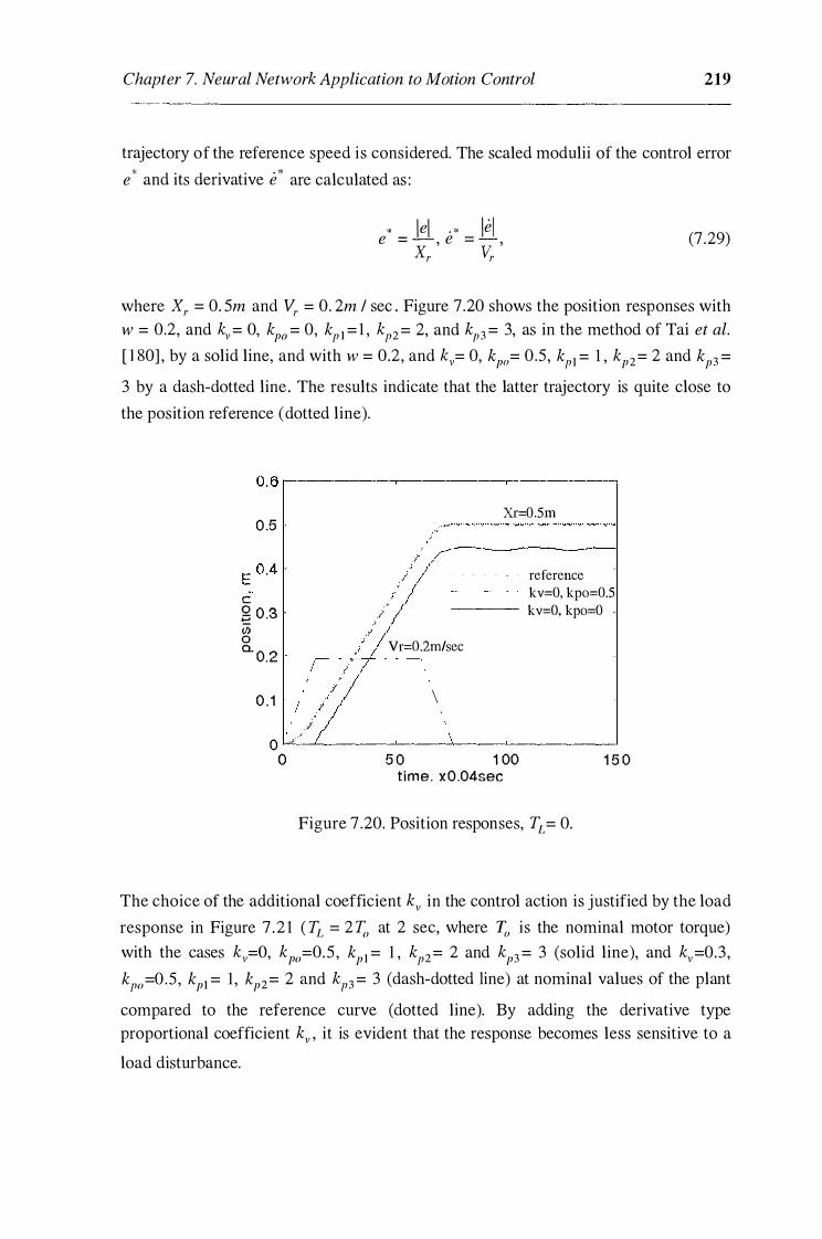
Chapter 7. Neural Network Application to Motion Control 219
trajectory of the reference speed is considered. The scaled modulii of the control error
e '" and its derivative e * are calculated as :
* \e\ · * lei e = -, e = -, xr vr
(7 .29)
where Xr = 0. 5m and Vr = 0. 2m I sec . Figure 7.20 shows the position responses with
w = 0.2, and kv= 0, kpo = 0, kP 1 = 1 , kP2 = 2, and k113 = 3, as in the method of Tai et al.
[ 1 80] , by a solid line, and with w = 0.2, and kv= 0, kpo= 0.5, kP1 = 1 , kp2= 2 and kp3 =
3 by a dash-dotted line. The results indicate that the latter trajectory is quite close to
the position reference (dotted line).
0.6r---------��--------�----------�
0 .5
c g 0 .3 ii) 0 0.. 0.2
0 . 1 , ./ I ,/
0 ,,
0
.> i
/ .!
/ · ' ./
Xr=O.Sm
reference kv=O, kpo=O.S
---- kv=O, kpo=O
Vr=0.2m/sec
\
5 0 1 00 1 5 0 t ime. x 0.04sec
Figure 7 .20. Position responses, TL = 0.
The choice of the additional coefficient kv in the control action is justified by the load
response in Figure 7 .2 1 ( TL = 2T0 at 2 sec, where I;) is the nominal motor torque)
with the cases kv=O, kp0=0.5 , kp1 = 1 , kP2= 2 and kp3 = 3 (solid line), and kv=0.3,
kP0=0.5 , kp1 = 1 , kp2= 2 and kP3 = 3 (dash-dotted line) at nominal values of the plant
compared to the reference curve (dotted line). By adding the derivative type
proportional coefficient kv , it is evident that the response becomes less sensitive to a
load disturbance.

Chapter 7. Neural Network Application to Motion Control
0.6 .---------�----------�--------�
0.5
c � 0.3 (I) 0 0..
0.2
0 . 1 I
. '/
Xr=0.5m
reference � - - kv=0.3, kpo=0.5
--- kv=O, kpo=0.5 TL=2To
1 Vr=0.2m/sec ,-- - - - - - - \
I I I \
0 �--------�----------�--------� 0 5 0 1 00 1 5 0
t im e. x0.04sec
Figure 7 .21. Position responses, TL = 2T0 at 2 sec.
220
Robustness of the proposed approach is verified through the cases of structured and
unstructured uncertainties. The tracking responses to the optimal trajectory of the reference speed where m = 2m0 , L = 0. 5L0 , and TL = 0. 5�� (1 + sin l Ot) , (m0 and L0
are nominal values of the load mass and chain length), are shown in Figure 7 .22, and where an initial swing <Po of 75 degrees is applied to the crane model, in Figure 7.23.
0 . 6
0 .5
0 .4
E c: 0 .3 0 e U) 0.2 0 a..
0 . 1
0
-0. 1 0
Xr=0.5m
. . . ;;:/"--/>·>-·�-�f�----/1 / - - - ·· - reference
/ - - - - kv=0.3, kpo=0.5
/ J' .I ---- kv=O, kpo=O
·' Vr=0.2m/sec
\
5 0 1 00
ti m e , x0 , 04sec 1 5 (
Figure 7 .22. Position responses, m = 2m0 , L = 0. 5L0 , and 1� = 0. 5J;J l + sin 10t) ;
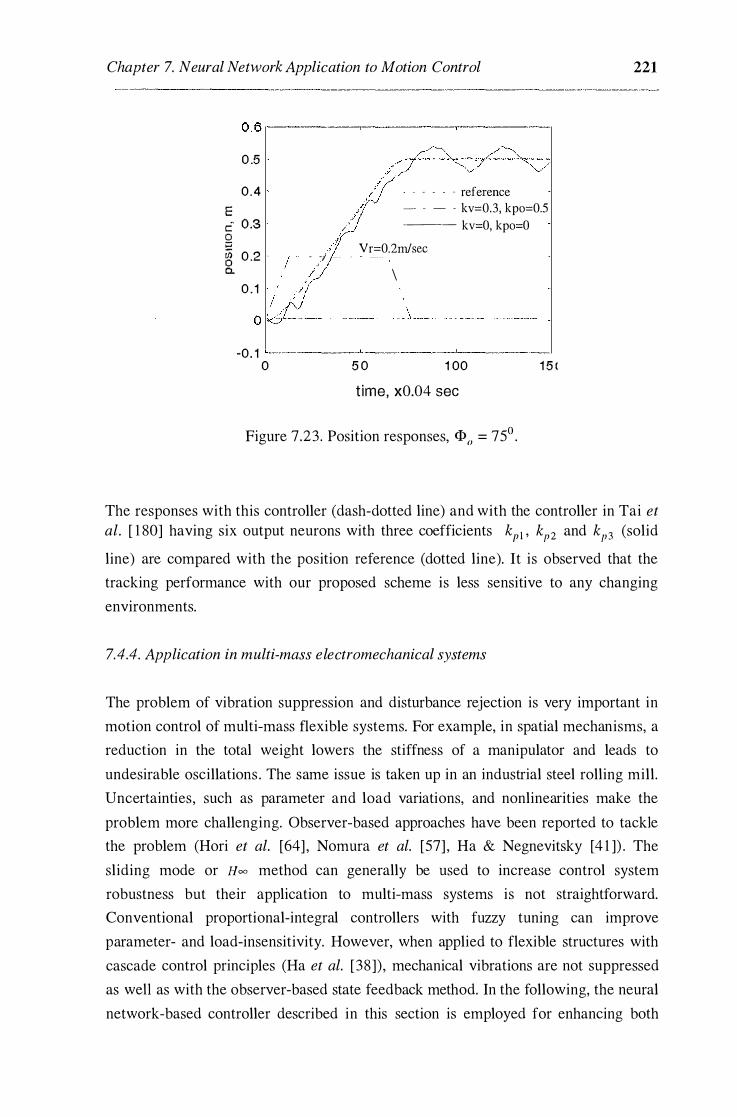
Chapter 7. Neural Network Application to Motion Control
0 . 6 .---------�--------�--------�
0 .5
0 . 4
E c:� 0.3 0 ;::; � 0 .2 a..
0 . 1 I
,- - :J I ·' j
f
/;/::�.�-!' '
I - - - - - reference
-- - - - kv=0.3, kpo=0.5
/. --- kv=O, kpo=O
Vr=0.2m/sec
\
\
-0 . 1 '---------'----------'---------' 0 5 0 1 00 1 5 (
t ime, x0.04 sec
Figure 7.23. Position responses, <1>0 = 75° .
221
The responses with this controller (dash-dotted line) and with the controller in Tai et al. [ 1 80] having six output neurons with three coefficients kpl , kP2 and kP3 (solid
line) are compared with the position reference (dotted line). It is observed that the
tracking performance with our proposed scheme is less sensitive to any changing
environments.
7.4.4. Application in multi-mass electromechanical systems
The problem of vibration suppression and disturbance rejection is very important in
motion control of multi-mass flexible systems. For example, in spatial mechanisms, a
reduction in the total weight lowers the stiffness of a manipulator and leads to
undesirable oscillations . The same issue is taken up in an industrial steel rolling mill.
Uncertainties, such as parameter and load variations, and nonlinearities make the
problem more challenging. Observer-based approaches have been reported to tackle
the problem (Hori et al. [64] , Nomura et al. [57] , Ha & Negnevitsky [4 1 ]) . The
sliding mode or Hco method can generally be used to increase control system
robustness but their application to multi-mass systems is not straightforward.
Conventional proportional-integral controllers with fuzzy tuning can improve
parameter- and load-insensitivity. However, when applied to flexible structures with
cascade control principles (Ha et al. [38]), mechanical vibrations are not suppressed
as well as with the observer-based state feedback method. In the following, the neural
network-based controller described in this section is employed for enhancing both

Chapter 7. Neural Network Application to Motion Control 222
robustness and the capability of vibration suppressiOn (Ha [45]) . An interesting
feature of the proposed neural network -based method is that the net plays the role of a
classifier to cluster the groups of the control error e and its time derivative e without
having to learn the system inverse dynamics. Correspondingly, an appropriate
command signal is generated to cause the servo output to follow a prescribed
trajectory. The two-mass servo system of Example 3.2 is used here as the controlled
object. Simulation results verify the validity of the proposed approach when applied
to flexible structure systems. The system block diagram including the neural network
based controller is shown in Figure 7.24. The speed reference is an optimal
trapezoidal trajectory. The load speed and acceleration feedback signals can be
indirectly estimated by an observer.
NNBC
25
/4.21 s+ 0 .01 s+ 1
Prefi lter SP
back emf
constant
Figure 7.24. Block diagram of a two-mass servo system with
a neural network-based controller (NNBC).
Simulation results are shown in Figures 7.25 - 7.27 where the reference and actual
speed is represented by a dash-dotted and solid line, respectively. Parameter insensitivity is verified in the case of load inertia variation, h = 2h,nom · Figure 7 .25
plots the time optimal process of the load speed response in this case.

Chapter 7. Neural Network Application to Motion Control
1
0 .5
' - - - .. - -r -.. �. -- � -::::r-"-"'"'"�"-·-----;----·-----R..- - -- - .. - - -- - -
� ' • ' : '· ' ' ' : 1\
' ' ' ' ' - - ] - - - - - - - - � - - - - - - - - - - - - - � - - - - - - - - - - - - - � - - \- - - - - - - -
' ' ' ' ' ' ' ' '
' ' ' ' ' ' I I I 'I 0 - - - - - - - - - .. - - -{ - - - - - - - - .. -- - - � - - - - - - - - - - - - -}-- - - - - --- --"' ' ' '
0
1
0 .5
2 0
' ' ' ' ' '
4 0 60
(a)
�� ' • '
: \ ' ' '
: \ '
I I I 'lo
80
- 7 - - - - - - � - - - - - - - - - � - - - - - - - - - � - 1 - - - - - -, ' '
I I I I � ' ' l : : ' ' ' '
0 � - - - - - - - -,- - - - - - - - - � - - - - - - - - - r - - - _\ ___ ......
0 2 0
' ' '
4 0
(b)
60 80
Figure 7 .25 . Speed response with load inertia variation, J 1 = 2 h,nom : (a) NN-based control, and (b) PI control.
223
The time optimal process of the speed response when a load torque disturbance, T1 = TL,nom exerted at t = 40 sec , is shown in Figure 7.26 to demonstrate the system
robustness against a load variation.
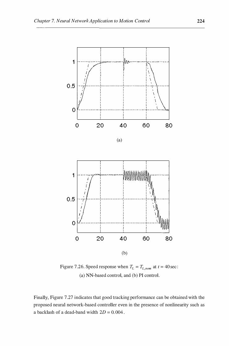
Chapter 7. Neural Network Application to Motion Control
1 � I I I
: \ I I I : '1. I > I I I 0 .5 " "] - - - - - - - - � - - - - - - - - - - - - - � - - - - - - - - - - - - - � - - t· · - - - - - -
I I I I I I
0 - - - - ... .. - - - .. -- � .. - .. - - - - - .. .. .. � -� .. .. ... - - - - .... - .... -�- - .. .. .. ,}_
0
1
0 .5
0
0
I I I I I I
2 0 4 0 6 0
(a)
I I : I : I
- - 7 - - .. .. .. - -- �-- - -- - - - - - - - -� .. - - - - - - - - - .... - � - - � -1 I I I I I
I
I I I I I I I I I I 1\ -- .. - - - .. .. - - - �-- .. - - - - - - - - - - � - - - .. - - - .... - - - - :- - - - - - ... ... I I I
2 0 4 0 60
(b)
80
80
Figure 7 .26. Speed response when TL = TL nom at t = 40 sec :
(a) NN-based control, and (b) PI control.
224
Finally, Figure 7.27 indicates that good tracking performance can be obtained with the
proposed neural network-based controller even in the presence of nonlinearity such as
a backlash of a dead-band width 2D = 0. 004 .

Chapter 7. Neural Network Application to Motion Control
' ' 1 --.---�___,_- - - - - -- - - - - -' '
' ' I I o, ' ' ' 0 .5 - -7 - - - - - - - - � - - - - - - - - - - - - - � - - - - - - - - - - - - - � � - , - - - - - - - -
: : : I ' ' ' ' ' ' ' ' ' ' ' ' ' ' ' I I I � ' I I I ' ' ' \ 0 - - - - .. .. .. -- .. - - -: - - - - - - - - .. - - - -� .. - - - - - - - - - - - -:- - - -- ... - -·- -H-' ' '
1
0 .5
0
' ' ' ' ' ' ' ' '
2 0 4 0 6 0
(a)
1 : : : I ;. I I I '•
l : : : \ I I I I I
I : : : \
-�'- - - - - - _:_ - - - - - - - - J - - - - - - - - - L - �
I I I I I
: : : � 0 - - - - - - - - -:- - - - - - - - - -: - - - - - - - - - r- - - - -
0
' '
2 0 4 0
(b)
60
80
80
Figure 7 .27 . Speed response with backlash 2D = 0. 004 :
(a) NN-based control, and (b) PI control.
225
Comparing the responses obtained by the proposed method (Figures 7 .25(a), 7.26(a),
and 7.27(a)) and the conventional cascade control with proportional-integral (PI)
controllers (Figures 7 .25(b), 7-26(b), and 7.27(b)) at the same conditions
demonstrates its feasibility in applications to flexible systems for vibration
suppression and high tracking performance even in the presence of parameter and
load variations, and nonlinearity .

Chapter 7. Neural Network Application to Motion Control 226
Note that the proposed neural network-based controller is designed like a
proportional-derivative fuzzy logic controller. This explains the robustness of the
control system. The attraction here is that no fuzzy logic operations and no a priori
knowledge of the plant dynamics are required. Further research may focus on the
application of an additional feedforward compensation, or some adaptive schemes for tuning the coefficients kpi , i = 0, 1, 2, 3 , and kv to cope well with severe uncertainties
in flexible structures.
A neural network-based controller has been proposed for servo tracking with high
accuracy and robustness . The neural net serves as a classifier to cluster the control
error and change of error groups instead of acting as the inverse of the plant. Control
knowledge is embedded into the representation of the net and helps to generate the
appropriate control signal for tracking systems that can cope well with uncertainties.
By noticing the symmetry in the control actions and taking the rate of change of error
into account, the neural network structure obtained is rather simple and the tracking
process is robust against any uncertainties. The attraction of the proposed controller is
that no a priori knowledge of the controlled object and its dynamics is required, thus
it can be applied to a variety of linear or nonlinear servo applications. Simulation
results are provided for the control of an overhead crane model. The proposed
approach can be applied to the control of a two-mass servo system. Simulation results
indicate the capability of vibration suppression and high tracking performance even in
the presence of parameter variation, load torque disturbance, and backlash
nonlinearity combined with the gear torsion. A learning scheme for the choice of the
controller coefficients and the proposed approach application to industrial servo
systems working in severely changing environments can be subjects for future
extension.
7.5 Robust control using neuro-fuzzy approach
In some motion applications, controlled systems are subject to inertia variations and
load torque disturbances. In robot drive systems, several motion axes are
mechanically coupled and the position of one axis usually affects the inertia of the
others . It is known that the dynamic model of a manipulator is highly non-linear and
requires a knowledge of the kinematic dynamics and inertia parameters . Normally, the
inertia parameters are not available from manufacturers. On the other hand, in
robotics, the plant model, depending on inertia parameters, is highly nonlinear and the
values of inertia parameters are required for most modern control schemes that

Chapter 7. Neural Network Application to Motion Control 227
incorporate inverse dyn amics. There are several approaches for identifying the inertia
parameters of manipulators and to minimise the number of the inertia parameters
appearing in their mathematical equations. A survey on approaches based on this
technique is given in Lin [ 1 8 1 ] . However, the inconvenience of these methods are that
the closed form of the system with the inverse dynamics is difficult to analyse, and a
large number of off-line experiments are needed to find the required parameters.
Recently, there has been increasing interest to implement neural network and fuzzy
techniques to address these problems, with robot drive systems as the controlled
object. In Lee et a!. [ 1 82], an inverse nonlinear controller using neural networks is
applied to treat the position control problem in servomechanisms with nonlinear
dynamics. An additional parallel neural network is used in Lee et al. [32] to enhance
adaptive properties of the basic fixed neural network-based inverse nonlinear
controller described in [ 1 82]. These techniques were shown to be capable of
providing high performance closed-loop control for several classes of
servomechanisms with nonlinearities . Here, a training data set consisting of the
system output vector ( q( t) q( t) q(t)l and the control input u(t) is used for modelling
the dynamic behaviour of the nonlinear system, where q represents an appropriate
output of the system such as an angular signal if the described system is a position
control servomechanism. For this case, neural networks of the radial basis function
type are utilised. Doschner & Schneider [ 1 83] proposed a neural network approach
for learning the inverse dynamics of a robot, using Kohonen feature maps [ 1 84] based
on the training data set of all available robot coordinates.
In real time control with neural network applications, it is assumed that the modelled
system characteristics are accurately approximated by the net. However, this
assumption can be made only after appropriate training and with a sufficiently large
number of neurons. When learning the inverse characteristics of the plant from zero,
the neural net must be trained off-line, applying the plant input and output signals. For
this, we need a robust system which is able to cope with all nonlinearities in order to
provide the required training data set. This section is devoted to a technique
developed in Palis, Ha et a!. [33] , [ 1 65] using :
• fuzzy logic control to guarantee stability during off-line training operations,
• a neural network approach to identify the inverse characteristics of the nonlinear
dynamics in order to compensate for nonlinearities in the feedforward channel, and
• a feedforward neural network model to cope with parameter variations due to an
inaccurate approximation of mechanical parameters.

Chapter 7. Neural Network Application to Motion Control 228
7. 5. 1 . Robustness against parameter variations with fuzzy control
Let us assume that the plant consists of p axes of motion which are influenced by the
interaction of forces dependent on the co-ordinates of the other axes. The load torque,
Tv and moment of inertia, 1 , can then be generally written by
TL = TL (x) and J = J(x) , (7 .30)
where x = (x 1 , x2 , . . . , xP l is the state vector. Considering the i-th axis with the
coordinate
and using the second equation of Lagrange
the following equation can be obtained:
dw _ o1 dxj 1- - Tgen - w I.�- - TL , dt . ox . dt J J
(7.3 1)
(7 .32)
(7 .33)
where r; = I�en - Tv Tf?en i s the generating torque, and Wkin and �,01 are the kinetic
and potential energy, respectively.
It is obvious that the speed control has to cope with considerable parameter variations.
When compensating for these influences, the drive system can be decoupled and
optimal dynamic behaviours of the speed loop can be achieved. For this purpose, an
adaptive fuzzy observer is proposed in Palis & Ha et al. [33 ] and an observer-based
fuzzy tuner in Palis & Ha et al. [ 1 65 ] .
A. Decoupling of the motion axes using adaptive fuzzy observers
In electrical drives, it can be assumed that the torque generating a current component
is controlled by means of an inner current loop. Therefore, we have a similar structure
for the cascaded speed loop of DC- and AC-drives. The proposed control system is
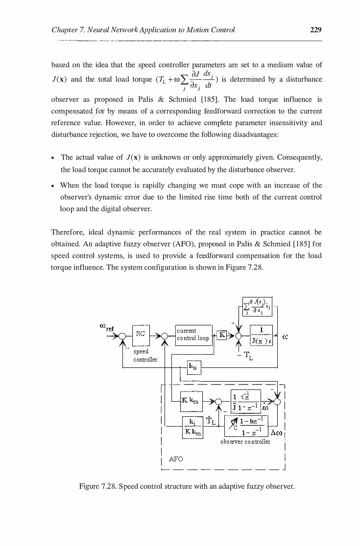
Chapter 7. Neural Network Application to Motion Control 229
based on the idea that the speed controller parameters are set to a medium value of ()J dx .
J(x) and the total load torque ( TL + ffi 'L--.1 ) is determined by a disturbance ' ax . dt J .I
observer as proposed in Palis & Schmied [ 1 85] . The load torque influence is
compensated}or by means of a corresponding feedforward correction to the current
reference value. However, in order to achieve complete parameter insensitivity and
disturbance rejection, we have to overcome the following disadvantages:
• The actual value of J(x) is unknown or only approximately given. Consequently,
the load torque cannot be accurately evaluated by the disturbance observer.
• When the load torque is rapidly changing we must cope with an increase of the
observer's dynamic error due to the limited rise time both of the current control
loop and the digital observer.
Therefore, ideal dynamic performances of the real system in practice cannot be
obtained. An adaptive fuzzy observer (AFO), proposed in Palis & Schmied [ 1 85] for
speed control systems, is used to provide a feedforward compensation for the load
torque influence. The system configuration is shown in Figure 7.28.
speed controller
current co ntrol lo op
"a J(x .) . l..t �1 Xj j a x j
- - - - - - --=-- � -1 I 1 -c z
J' 1 - z- 1 ro I I � 1 - bz-1 I C 1 - 1 A - z uro l
obs erver co ntroller I I I AFO I .__ _ _ _ _ _ _ _ _ j
Figure 7.28. Speed control structure with an adaptive fuzzy observer.
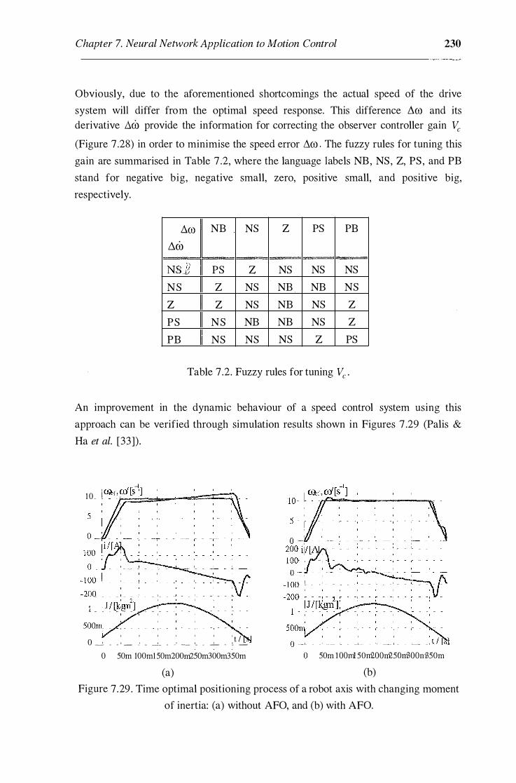
Chapter 7. Neural Network Application to Motion Control 230
Obviously, due to the aforementioned shortcomings the actual speed of the drive
system will differ from the optimal speed response. This difference Llro and its derivative .6.ro provide the information for correcting the observer controller gain Vc (Figure 7 .28) in order to minimise the speed error .6.ro . The fuzzy rules for tuning this
gain are summarised in Table 7 .2, where the language labels NB, NS, Z, PS , and PB
stand for negative big, negative small, zero, positive small, and positive big,
respectively.
ilro NB NS z PS PB
ilm N88 PS z NS NS NS
NS z NS NB NB NS
z z NS NB NS z PS NS NB NB NS z PB NS NS NS z PS
Table 7 .2. Fuzzy rules for tuning Vc .
An improvement in the dynamic behaviour of a speed control system using this
approach can be verified through simulation results shown in Figures 7 .29 (Palis & Ha et al. [33]) .
-l
10_ l <0r:F,oi�[s�·]�==-...�---===�
I I I I I I I t I 0 -� _ _ I -· .� _ _ __!__ _ _1 -- I_ _ � _ .!_ _
0 50m 100m1 50m200m250m300m350m
(a)
50m 1 OOml 50r&OOnQ50rmOOni350m
(b)
Figure 7 .29 . Time optimal positioning process of a robot axis with changing moment
of inertia: (a) without AFO, and (b) with AFO.

Chapter 7. Neural Network Application to Motion Control 231
Here, the time optimal positioning process of a robot axis is considered when the load
torque and moment of inertia are changing. The speed response with AFO achieves
better performance thanks to the compensation for the disturbance influence in the
observer control loop which is adaptively adjusted by a fuzzy logic rule set.
B. Decoupling of the motion axes using observer-basedfuzzy tuning
In the previous chapter, fuzzy tuning of the feedforward compensation signal from a
disturbance observer has been shown to offer good possibilities for improving load
and- parameter insensitivity . As an alternative to the adaptive fuzzy observer
mentioned above, fuzzy tuning schemes can be incorporated to improve robustness
against parameter and load variations in the system of Figure 7.28. Here the
parameters of the PI controller in the observer control loop will be tuned according to
some simple fuzzy logic schemes, proposed in Ha [ 1 12] . Figure 7.30 shows the drive
system including a PI controller with fuzzy tuning in the observer feedforward loop.
The total load torque is compensated for using a disturbance observer-based fuzzy
tuner (DOFT).
speed controller
current co ntrol lo op
1 t J(x ) s - TL
- - - - - - - -, -1 I 1 "C z
1 1- z- 1 ro I I � 1 -Jfz-t I C - 1 A 1 - z uro I digital PI-controller I 1 mth fuzzy tuning I I DOFT
.__ _ _ _ _ _ _ _ _ j
Figure 7 .30. Speed control with disturbance observer-based fuzzy tuner (DOFT).

Chapter 7. Neural Network Application to Motion Control 232
The tuning expressions (5.8)-(5 . 1 0) are applied for adjusting the parameters Vc and b
of the PI controller in the system of Figure 7.30. The salient features of the use of the
disturbance observer-based fuzzy tuner approach are:
• fuzzy logic can be introduced to continuously change the controller gain and time
constant, depending on the control error and its rate of change,
• the rule base for tuning is based on human expert experience rather than on precise
information of the plant dynamics and allows an easy modification,
• tuning schemes result in explicit expressions which allow low computational cost
and a simple implementation.
High performance of a speed control system using this approach can be verified
through simulation results shown in Figure 7.3 1 and 7.32 (Palis & Ha et al. [ 1 65]) .
The time optimal positioning process of a robot axis is considered when the load
torque and moment of inertia are changing. Comparing the speed responses of Figure
7 .3 1 and Figure 7.32 demonstrates the priority of fuzzy tuning schemes for robust
tracking improvement.
speed
1 �... . . . . . . . . . 1: � :� . . . . . . . . . . . . . . . . :l' . . . . . . . . . . . . . . . ·. j 0.5 u� =@fuu uu uu+� ��+ u O u uuU
0 ===·:· . . . . . . . . . . . . . . . . ��·-t-!-;-----'""""i=
_::FIE:E=I i 1 1 � � 0=
0 0.5 1 1 .5 2 t [ s ]
Figure 7 .3 1 . Time optimal positioning without fuzzy tuning.

Chapter 7. Neural Network Application to Motion Control
1 g· · · · · · · · . . · · ,·
speed�· . . . . . . . . . . . . . . . . . .
, .
.
. .
. . . . . . . . . . . . . .
1 0.5 =·•l • • • • u • • • • • • • • • • l • • • u ••• • • • � • • l • • • • u • • • o • • • • u 0 -----=� · - : · · . . · · · · · · · · · · · · - �""-"""!-: ------1=
: I 2�� : : 1 �= 0 ___:__-�-� 0 0.5 1 1 .5 2
time
Figure 7 .32. Time optimal positioning with fuzzy tuning.
7. 5.2. Robustness enhancement using a neural network model for the inverse
dynamics
233
As shown in the section above, fuzzy logic controllers are able to cope with non
linearities and to guarantee stability in a wide range of parameter variations . However,
it should be clearly pointed out that both large and fast changes of inertia lead to an
increasing error in the estimated torque value from the observer. A neural network
identifier can be incorporated in order to alleviate the influence of the nonlinear
mechanism characteristics due to inertia variations. Here, a parallel neural network
model for the inverse dynamics (NNMID) is applied to the system with AFO or
DOFT to provide information of the system input depending on the output. The
following approach is proposed:
(i) Set up a neural network with the set
(7 .34)
as inputs and the control signal uN (k) as the desired output of the NNMID, and
train the net using real data sets of the system.

Chapter 7. Neural Network Application to Motion Control 234
(ii) Once a good fit is obtained, the resulting neural network actually realises the
function
uN (k) = f(w(k), w(k - 1 ) , w(k - 2), uN (k - 1)) ,
and inserts it into the system to calculate the control signal uN (k) .
A schematic diagram of the described control system is given in Figure 7.33
- speed controller
current conlrol locp
.- -
1
- 1 I I I I
J( X ) s � I
(7 .35)
Figure 7 .33 Speed control structure with an additional neural network model.
In recent literature, for example Hunt et al. [ 1 68], Widrow & Lehr [ 15] , Pham & Xing
[23] , a variety of neural networks have been proposed. Among non-dynamic
networks, radial basis function (RBF) ones seem to be very promising. As noted in
Section 7 .3 , an important advantage of RBF networks is that they can be trained in a
fraction of the time it takes to train back-propagation networks or multilayer
perceptrons with similar power and generality (Van den Bout & Miller [ 1 86] ,
Peterson [ 1 87]) . Furthermore, Lyapunov based updating laws as used in Lee et al.
[32] can be designed for network training to guarantee asymptotic convergence of the
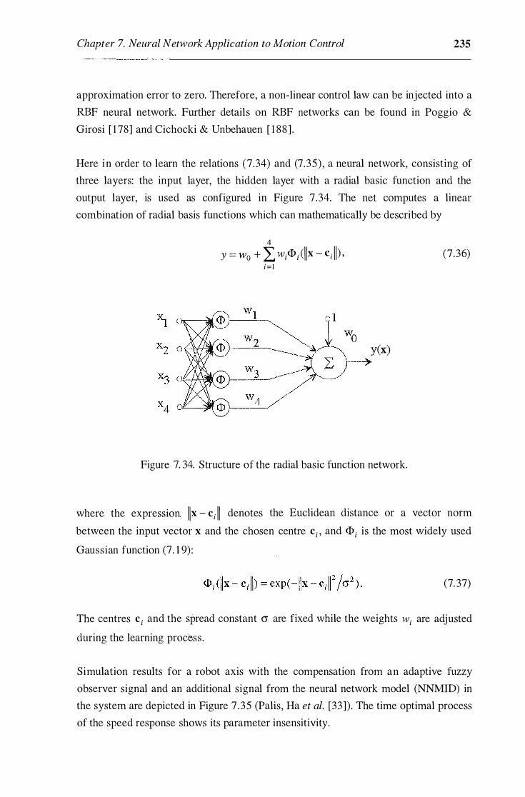
Chapter 7. Neural Network Application to Motion Control 235
approximation error to zero. Therefore, a non-linear control law can be injected into a
RBF neural network. Further details on RBF networks can be found in Poggio & Girosi [ 178] and Cichocki & Unbehauen [ 1 88] .
Here in order to learn the relations (7 .34) and (7 .35) , a neural network, consisting of
three layers: the input layer, the hidden layer with a radial basic function and the
output layer, is used as configured in Figure 7.34. The net computes a linear
combination of radial basis functions which can mathematically be described by
4 Y = Wo + L wi<Pi CI Ix - ci ll) , (7.36)
i=l
y(x)
Figure 7. 34. Structure of the radial basic function network.
where the expression l lx - ci II denotes the Euclidean distance or a vector norm
between the input vector x and the chosen centre ci , and <Pi is the most widely used
Gaussian function (7 . 1 9) :
(7.37)
The centres ci and the spread constant cr are fixed while the weights wi are adjusted
during the learning process.
Simulation results for a robot axis with the compensation from an adaptive fuzzy
observer signal and an additional signal from the neural network model (NNMID) in
the system are depicted in Figure 7 .35 (Palis, Ha et al. [33]) . The time optimal process
of the speed response shows its parameter insensitivity.

Chapter 7. Neural Network Application to Motion Control
speed . . . . . 5 . . . . . . . . . . ' . · · · · · · · · : · · · · · . . . . . . r . . . . . . . .. . i" . .. . . . . . . r . . . . . . . . . . f . . . .. . . . . . . i . . . . . . . . . . . .. . . . . . . . . ! . . . . . . . . . . . ' . . .
0.05 0.1 0. 1 5 0.2 0.25
200 · · · · · · · · · · i " " " ' " ; · · · · · · · · · ·i· . . . . . . . . . . . ! . . . .. . . . . . . . t · · · · · · · · · . . i · · · · · · · · · · · i · · · . . · · · . . · j · · · · · · · · " · j· · · · · · · · · ·
current : : : : : : ; ; ; . . . . . ' l a9'
0 · · · · · · · · · ·i
· · · · · · · · · · · : . . . . . . . . . : . . . . . . . . . . . ; . . . : . . . . . : . . . . . . . . . · i · · · · · · · · · · · i . . . . . . . . . . . ; . . . . . . . . . -200 . . . . . . ) . . . . . . . . . +==
0 0.05 0.1 0 . 1 5 0.2 0.25 2 . . . . . . . inertia l j j l l l j i l . . ' . ' ' . ' '
:= 0 0.05 0.1 0. 1 5 0 .2 0.25 t [ s 1
236
Figure 7.35 . Time optimal positioning process with a changing moment of inertia
when using AFO and NNMID.
Robustness enhancement can also be verified with the use of DOFT augmented with
NNMID as shown in the simulation results of Figure 7.36 (Palis, Ha et al. [ 1 65]) . The
time optimal speed response exhibits good tracking performance in a wide range of
inertia variation. It is observed that the network output signal dominates the speed
controller output. Thus in the presence of severe parameter variations, the main
correction is accomplished by the neural network model. The results obtained indicate
that the proposed neuro-fuzzy approach can be a promising method to overcome the
ill effects of wide ranging parameter variations.
This section has presented a fuzzy and neurocontrol approach for drive systems with
ch,anging parameters and load. The influence of load and inertia variations is
alleviated using an adaptive fuzzy observer or a digital observer-based fuzzy tuner.
Taking into consideration a large range of inertia changes associated with severe
nonlinearities , an additional compensation signal from a neural network model for
inverse dynamics is added to the control signal. Thus, the closed-loop system is made
more robust. Simulation results of a time optimal positioning process verify the
validity of the proposed method.

Chapter 7. Neural Network Application to Motion Control 237
i n erti a
1 '1 . 5 2
2 · · · · · =-= :.·.:.: · sp$Jed· contro H �r ·outptlt · - - ·
-- net outptlt � 0
- 2 0 0 . 5 1 1 . 5 t ime 2
Figure 7 .36. Time optimal positioning process with changing moment of inertia when
using DOFT and NNMID.
7.6 Summary and discussion
Artificial neural networks, inspired by biological nervous systems, are composed of
many elements operating in parallel. The network function is determined mainly by
the connection between elements . A neural network can be trained to perform a
particular functions by adjusting the values of the connection weights between
elements. In this chapter, the basic concept of artificial neural networks was briefly
introduced and their applications to motion control system has been outlined. Its
content focused mainly on the use of a neural network to mimic a nonlinear controller,
e.g. a fuzzy logic controller; or to cluster the groups of both the servo control error
and its derivative which an appropriate control action would correct. The combination
of fuzzy and neurocontrol was proposed as a promising approach to the problem of
severe sensitivity when system parameters and load varying a wide range.
Since a neural network can approximate and learn any control relationship of practical
interest, it is worth exploring the implementation of a fuzzy logic controller's input
output relationship in a neural network to ease the control system of computation
burden. The solution is investigated with reference to the position control of a

Chapter 7. Neural Network Application to Motion Control 238
swinging load of an overhead crane model . A radial basis function network, , -��( ( .'! ,' /"!{J ' I
undergoing a two-stage (transient and steady-state) training process, approximates the
control action from a fuzzy logic controller for that model . Simulation and
experimental results, compared with those of the system with the fuzzy logic
controller, show the neural network ability to control in the same manner as a fuzzy
logic controller. Robustness against parameter and load variations has been verified.
Another contribution of this chapter is an application of the back propagation network
to the tracking control of servo drive systems. Based on information of the control
error and its time derivative, the neural network can classify the error and change-of
error patterns, and generate t,he appropriate control action without learning the inverse
dynamics of the plant. The llierit of the proposed approach lie in the design simplicity
and its practicality for real-time implementation with a look-up table. The overhead
crane model and the two-mass servo drive, mentioned in previous chapters, is used as
the controlled objects with the standard time optimal trapezoidal trajectory for
tracking. Simulation results indicate that the systems exhibit highly robust
performance in the presence of uncertainties in the plant parameters and control
process . It can be noticed that the proposed approach is conceptually analogous to the
proportional-derivative like fuzzy logic control (see Section 4.4. 1 ) without elaboration
on membership functions and fuzzy logic operations.
For servomechanisms w ith severe nonlinearities, the fuzzy neurocontrol technique has
been presented. It combines salient features of observer-based fuzzy control for
decoupling motion axes , and of additional compensation from a neural network model
for inverse dynamics to provide adaptive enhancements. In the observer control loop,
the influence of an unknown equivalent load torque is compensated for by an adaptive
fuzzy observer controller with the feedforward gain adjusted from a fuzzy rule set.
Alternatively, fuzzy tuning schemes can be used to continuously change the gain and
time-constant of the disturbance observer-based controller. A radial basis function
neural network is trained to provide information of the input (control action) in
relation with the system outputs (plant states) in the proportional-integral-derivative
manner. The neural net then provides a parallel compensation action for a wide range
of system's uncertainties and nonlinearities. The effectiveness of the proposed
approach has been demonstrated in simulation results of the time optimal positioning
process of a robot axis .

Chapter 7. Neural Network Application to Motion Control 239
Although the field of neural networks has attraction of some five decades, it has found .
solid application only since the early 1980's. Thus, it is still very much in its infancy
compared with the other fields of control systems. Many questions still have to be
answered: determining the best network topology, choosing the net parameters, and
number of neurons required, for example. Neural network application to motion
control systems needs further exploration. Theoretically, dynamic networks can be
used as universal identifiers and sophisticated controllers. However, static networks
possess proven capabilities of arbitrary function approximation which can be
practically exploited in the context of motion control using state feedback and
feedforward compensation. The attraction of using the neural network instead of other
model forms within the control strategy is the ability to effectively represent complex
nonlinear systems.
Chapter 8
Summary and Future Extensions
8.1 Introduction
This study has encompassed a variety of areas of research relating to robustness issues
in analysis and design of motion control systems, particularly electrical drives and
robotics . The problems of estimating the dynamic properties as well as damping
capability of a generalised electromechanical model, and the development of the
robust modal control for linearised drive systems have been addressed, using
conventional control approaches. The application of uprising artificial intelligent ,' ; ,' ' '
tools, namely fuzzy logic and neural network, brings new insights into robust
enhancement techniques.
Fuzzy logic control and fuzzy logic controllers were discussed with a case study of an
overhead crane modeL Fuzzy tuning schemes, which result in explicit expressions for
continuously changing the PI controller parameters or adjusting the control in the
sliding mode, have demonstrated their ability to significantly improve system
robustness. Robust modal control can also employ some fuzzy tuning schemes to cope
with a wide range of load and parameter variations. Predictive coefficients of an
unknown input observer were tuned taking into account the change of the estimated
disturbances. Conditional schemes were introduced to tune the dynamic feedforward
coefficient according to the signs of error and the change of the estimated load torque.
The robust feedback gain were adjusted according to the signs of error and of the
change of error. Simulation results for servo drive systems verified the effectiveness
of fuzzy tuning in robust modal control.
Some neural network based techniques have been proposed. A radial basis function
network was used to closely approximate the input-output relationship of a well
designed fuzzy logic controller. A backpropagation feedforward network was trained
Chapter 8. Summary and Future Extensions 241
to cluster the error and derivative-of-error patterns and correspondingly generate the
proper control action in tracking servo systems. Fuzzy and neurocontrol approach was
developed for systems with severe nonlinearites, using a neural network model for the
inverse dynamics in addition to an adaptive fuzzy observer or and disturbance
observer-based controller with fuzzy tuning. The neural network capabilities of
learning and approximating have been shown through the simulation and, partially,
experimental results. It is believed that neuro technique will be very promising for
robust control of motion systems.
In this final chapter, the important points encountered during the course of this study
are summarised, and a brief review of the results obtained is presented. A number of
extensions and areas of improvement which may be investigated in future work are
also outlined. The chapter is ended with some conclusion remarks.
8.2 Summary of main results
When analysing dynamic properties of pmlti-mass electromechanical systems, it is
required to have a common model for a variety of electrical drives with different types
of motors. The dynamic stiffness of a generalised electric motor's speed torque
characteristics, proposed by Kljuchev [5 1 ] , has a significant contribution to the
construction of such a model. The problem, albeit classic, is still timely when
considering flexible structures in robotics or space technology and the increasing
number of vector-controlled AC-motors which have a linearised decoupled model.
The elaboration on a normalised characteristic equation of an n -mass system was
given in Chapter 2. The conditions for maximal damping and complete damping were
determined in the general case. The values of the electromagnetic and
electromechanical time-constants at maximal damping were found in dependence on
the mass ratio (Ha [55]) . The results for two-mass systems, which are widely-known
in Soviet literature, can be derived as a special case of those obtained for a general n
mass case. The use of multi-parameter root loci allows considering other changing
factors , such as the electromagnetic time-constant and the mass ratio, and the
influence of viscous friction on the motor, load and coupling shafts . With a given
mass ratio, dominant root branches of the system root loci are observed not affected
by parameter variations as much as the branches containing other roots. While
dynamics of two-mass systems is sensitive to friction on the motor and coupling shaft,
maximal damping of the system is seriously affected by friction on the load shaft. The

Chapter 8. Summary and Future Extensions 242
oscillatory influence of viscous friction on the load and coupling shaft in two-mass
systems is reduced at large values of the mass ratio.
In order to design a controller for vibration suppression and load rejection in multi
mass servo systems, robust modal control, first proposed in Ha [9], was developed in
Chapter 3 . A methodical procedure for designing robust modal controllers was
presented. The dominant pole-based technique was proposed for one-mass and two
mass servo systems. When choosing the desired poles for determining the state
feedback gain, only the dominant root pair assigns the closed-loop system dynamics .
The other poles can be chosen according to additional conditions relating to accuracy
or damping capability. This may improve the steady-state performance of systems
with modal control . Design equations were given for servo systems to achieve
maximum damping. Vibrations due to backlash nonlinearity can be suppressed using
the proposed approach. On the other hand, an eigenvalue sensitivity analysis showed a
significant increase of the dominant root sensitivities in the vicinity of some critical
values of the drive parameters. For simultaneously estimating the unmeasurable states
and external disturbances, an observer was constructed on the basis of measurements
of the system input and output and some a priori information of the unknown inputs.
The proposed observer is able to estimate the torsional torque and load speed, and
load torque in a multi-mass servo system. Based on load torque estimates ,
feedforward compensation principles was applied to reject the disturbance influence.
Considering the parameter variation problem, a robust feedback signal was added to
the modal signal. When satisfying some matching conditions, the asymptotic stability
condition was determined via the second method of Lyapunov in dependence on the
bounds of uncertain matrices of the state model. Design procedures for the
continuous-time and discrete-time robust modal controllers were illustrated in servo
drive systems. Simulation results demonstrated the system parameter- and load
insensitivity, and also robustness against nonlinear backlash in the shaft gear of a two
mass servo system.
Fuzzy logic, a new way to represent the vagueness in everyday life, first introduced by
Zadeh [ 12] , and its application to control engineering was outlined in Chapter 4. As a
powerful tool to grasp the real world complexity, uncertainty, and unpredictability,
fuzzy logic has demonstrated its capability of robustness enhancements in many
systems including motion control ones. Fuzzy reasoning or approximate reasoning
was considered from the engineering viewpoint with IF-THEN fuzzy rules. The
design of a fuzzy logic controller was illustrated through the control of a crane model

Chapter 8. Summary and Future Extensions 243
with two main objectives, load minimal swing and robustness . Simulation and
experimental results confirmed the validity of fuzzy logic control in terms of robust
performance and advantage over conventional control techniques. The laboratory
model can be utilised for teaching fuzzy control issues to university students in
electrical engineering (Negnevitsky, Ha et al. [ 1 34]). Pros and cons of fuzzy control
approach were also discussed.
In Chapter 5, simple fuzzy tuning schemes were introduced to continuously change
the controller parameters or the control action in order to enhance robustness. The
gain and time constant of a conventional proportional-integral (PI) controller were
tuned according to some exponential functions, resulting from some engineering
heuristics with the use of fuzzy logic (Ha [ 1 12]) . System robustness was verified
through high performance of transient responses in changing environment conditions.
The results were extended to multi-loop cascade control with a fuzzy tuned PI
controller used in each loop instead of conventional one. Simulation results in a two
mass system indicated that fuzzy tuning can be applied to cascade controllers in
flexible electromechanical systems to increase robustness to some extent for
parameter and load variations, and nonlinearities . Fuzzy logic schemes were also
applied to tune the control action to deal with unmodelled dynamics in sliding mode
control . First, the equivalent motion was determined from the desired sliding
eigenstructure. The use of a switching gain based on the Lyapunov stability theory
guaranteed the reaching condition in the neighbourhood of the sliding surface. Fuzzy
tuning schemes were then employed to accelerate the reaching phase, reduce
chattering, and hence, improve robust performance (Ha [ 1 48]). The proposed
technique were applied to the control of a elastic drive system. Simulation results in a
servo two-mass drive demonstrated its validity. Here, the explicit expressions for
fuzzy schemes facilitated the computational implementation of the proposed
controller.
The methodology using fuzzy logic and some engineering heuristics to tune a
conventional controller's parameters was extended to robust modal control in Chapter
6. Simple tuning schemes were applied for continuously changing the predictive
observer coefficients , the feedforward controller coefficients, and the robust feedback
coefficients (Ha & Negnevitsky [37]). The predictive coefficients of an unknown
input observer were tuned taking into account the change of estimated disturbances .
As illustrated in estimating the load torque of a two-mass servo system, fuzzy tuning
improved observer robustness . Conditional schemes were given for tuning the

Chapter 8. Summary and Future Extensions 244
dynamic feedforward coefficient in relation to the signs of the error and the change of
the estimated load torque disturbance. Fuzzy tuned feedforward compensation
ameliorated robust performance of the control of a robot arm motion, and a two-mass
position drive. Other fuzzy schemes were also proposed to tune the robust feedback
gain according to the signs of the error and the change of error. Simulation results
obtained through the position control of a two-mass resonant system indicated the
feasibility of robust modal controllers with fuzzy tuning in flexible structures for
vibration suppression and load rejection.
Chapter 7 was devoted to the application of artificial neural networks to motion
control. It focused mainly on the use of a neural network to mimic a nonlinear
controller, e.g. a fuzzy logic controller; or to cluster the groups of both the servo
control error and its derivative which an appropriate control action would correct. The
combination of fuzzy and neurocontrol was proposed as a promising approach to the
problem of severe sensitivity when system parameters and load varying a wide range.
The implement�tion of a fuzzy logic controller's input-output relationship in a neural
network to �ase the control system of computation burden was investigated with
reference to the position control of a swinging load of an overhead crane model . A
radial basis function network, undergoing a two-stage (transient and steady-state)
training process, approximated the control action from a fuzzy logic controller for that
model (Ha & Negnevitsky [34]) . Simulation and experimental results, compared with
those of the system with the fuzzy logic controller, demonstrated the neural network
ability to control in the same manner as a fuzzy logic controller. Robustness against
parameter and load variations was verified. Another contribution of this chapter is an
application of the back propagation network to the tracking control of servo drive
systems. Based on information of the control error and its time derivative, the neural
network classified the error and change-of-error patterns, and generated the
appropriate control action without learning the inverse dynamics of the plant. The
merit of the proposed approach lie in the design simplicity and its practicality for real
time implementation with a look-up table (Ha [45]) . Simulation results for an
overhead crane model and a two-mass servo drive indicated that the systems exhibit
highly robust performance in the presence of uncertainties in the plant parameters and
control process. For servomechanisms with severe nonlinearities , the fuzzy
neurocontrol technique was presented, combining salient features of observer-based
fuzzy control for decoupling motion axes, and of additional compensation from a
neural network model to provide adaptive enhancements (Palis, Ha et al. [33]) . In the
observer control loop, the influence of an unknown equivalent load torque was

Chapter 8. Summary and Future Extensions 245
compensated for by an adaptive fuzzy observer controller or a disturbance observer
based fuzzy tuner. A radial basis function neural network was trained to provide
information of the input depending on the system outputs in the proportional-integral
derivative manner. The neural net then provided a parallel compensation action for a
wide range of system's uncertainties and nonlinearities . Simulation results of the time
optimal positioning process of a robot axis demonstrated the effectiveness of the
proposed approach.
8.3 Further extensions and developments
This thesis has touched a number of different areas of research including analysis and
synthesis of motion control systems. In each of these areas techniques have been
developed to address robust issues of electromechanical systems, such as electrical
servo drives and robotics . Despite the good achievements obtained from some of
these approaches, there is inevitably room for improvements and extensions within or
relating to the scope of this study.
8.3. 1 . Damping estimation
Through the standardisation and generalisation of the model of electromechanical
systems using the dynamic stiffness of the drive's speed-torque characteristics, it is
worth developing an expert system to help an electromechanical engineer to
determine damping and other dynamic properties of his system and provide further
guidance on choosing the appropriate controller design for it. Expertise obtained from
the results of Sections 2 .4 and 2.5 and the electromechanical product catalogue can be
embedded in the knowledge base and database which can be easily accessed and
updated. This knowledge base can be combined in an expert system for drive product
selection (Daoshen & Bose [ 1 89]) . A topic for further investigation may be the
estimation of maximal damping conditions in the presence of viscous friction and its
influence on the system dynamic properties. The robust root locus method, proposed
by Barmish & Tempo [61 ] , can serve as an effective tool for this purpose. The use of
the dominant pole pair leads to many interesting aspects in regards to the design of
robust controllers for motion control systems. One of these is the design aimed at
achieving maximal damping in electromechanical systems (Ha et al. [ 1 90]) . The
approach will be promising if it can be equipped with a self-organising mechanism to
assign the dominant roots.

Chapter 8. Summary and Future Extensions 246
8.3.2. Observer-based control and monitoring
Observer-based control techniques have prevailed their potential not only in control
strategies but also in conditions monitoring. Since robust performance of a system
with observer-based feedback and feedforward techniques depends much on the
accuracy of the recovery from unmeasurable states and external disturbances, observer
robustness is an important issue which requires further study. There is a possibility of
determining a linear robust control law when the full state cannot be measured and
observers are implemented to estimate the state (Jabbari & Schmitendorf [ 1 9 1 ]) .
Dynamic feedforward compensation in an adaptive manner may need to be extended
when the dynamics of the system subject to an unknown input is complicated. Robust
observers can also find applications in non-invasive fault incipient detection, as
shown in Ha & Negnevitsky [43] (see Appendix B). It is worth developing this
approach for vector-controlled AC drive systems on the basis of off-line or on-line
diagnostics. In general , solutions for a robust control strategy depends much on
uncertainty bounds, especially in robotics. A more reasonable choice of the bound of
the system uncertainty will lead to a less conservative solution. Thus, a study of
uncertainty bounds may be an interesting extension to robust control of robotic
manipulators (Man, Yu & Ha [ 192]).
8.3.3. Fuzzy logic control
Since the genesis of fuzzy logic and the " applications pull" of fuzzy logic control,
great progress has been made in constructing the mathematical foundation of fuzzy set
theory as well as developing tools for and demonstrating applications of fuzzy logic
control . However, the utility and role of fuzzy logic control remains controversial
because fuzzy logic, in the ordinary sense, is not a control design methodology. As an
implementation technique, fuzzy logic control needs more justifications of its use
from the user. A taxonomy was provided by Thomas & Armstrong-Helouvry [ 1 93] as
a contribution towards this purpose. Despite good performance obtained in many
simulations and experiments for fuzzy control systems, in fact, some important
theoretical and practical problems still have not been solved. For example, error
convergence, stability, and robustness have not been fully proven for fuzzy logic
control schemes to deal with system uncertain dynamics. Research tendencies aimed
at bridging that gap are open and very promising. Other attempts may focus on the
combination of fuzzy control with other control strategies, such as sliding mode

Chapter 8. Summary and Future Extensions 247
control (Ha & Negnevistky [ 1 94]) or neuromorphic control as mentioned in the
following section.
8.3.4. Neuro-fuzzy approach
A fuzzy inference system can now not only employ linguistic rules from human
experts but also adapt itself using numerical input/output data to achieve better
performance. In Jang & Sun [ 1 28], neural networks and fuzzy inference systems are
all special instances of adaptive networks called adaptive network-based fuzzy
inference systems. Once a fuzzy controller is transformed into an adaptive network, it
can take advantage of all techniques for designing a neural network controller,
namely, mimicking another controller, inverse control, backpropagation learning, and
others learning techniques. In general, setting up a common framework for unifying
both neural networks and fuzzy models will bring certain advantages over fuzzy or
neural networks approaches. For single-input single-output linearised systems, the use
of a fuzzy radial basis function network (Man, Yu & Ha [ 195]) to learn the system
uncertainty bound can result in an effective control strategy for robust tracking in
robotic manipulators . It is believed that by introducing some learning or self
organising algorithms i�to the disturbance observer-based fuzzy tuner, the neuro
fuzzy approach in Palis , Ha et al. [ 1 40] can be more flexible in order to cope with a
wide range of structured and unstructured uncertainties . Fuzzy tuning has
demonstrated its ability to ame'"fiorate robust performance of motion control systems,
neuro-fuzzy tuning with its learning capability will bring adaptive enhancements into
these robust systems.
8.4 Concluding remarks
A number of analysis and synthesis techniques addressing robustness issues of motion
control systems have been developed and verified. The conditions for maximal
damping and complete damping were derived from the general characteristic equation
of an n -mass system in dimensionless space. The multi-parameter root loci was used
to consider other changing factors, such as the electromagnetic time-constant and the
mass ratio, and the influence of viscous friction on the motor, load and coupling
shafts. The main centre of this study is involved in the application of modern control
and intelligent techniques to design robust controllers for electromechanical systems.
Robust modal control was examined with the emphasis on dominant pole-based
approach. A brief introduction to fuzzy logic control was provided with an ill ustrative

Chapter 8. Summary and Future Extensions 248
example for the control of an overhead crane model . Fuzzy tuning highlighted a
prominent possibility of robustness enhancements in conventional techniques such as
PI control, and also in s liding mode control and robust modal control . Neural network
approach was outlined in some applications exploiting the net ability to approximate
an input/output relation, to classify patterns of error and its derivative, and to learn the
inverse dynamics for an effective compensation.
The results obtained from this study can be directly applied to electrical drive systems,
multi-mass servomechanisms with backlash nonlinearity, and robot manipulators with
parameter and load uncertainties. However, the strategies proposed here are not
limited to electromechanical controlled objects. For example, robust modal control,
fuzzy tuning schemes, and neural network approach described in this thesis can find
applications in process control, biomedical technology, financial control problems, or
any dynamic system with severe uncertainties.
While the developments detailed in this thesis have touched many of the important
considerations relevant to robustness issues, especially the application of intelligent
tools, in motion control systems, the large scope of this area of research will be never
ever exhausted. Nor should the techniques proposed in this work be considered fully
complete. A number of possible future extensions and improvements have been
suggested in the previous section. More and more contributions to the pot-pdtu:ri of
this field are continually expected.

Appendix A
Normalised closed ... Ioop polynomials
There exist many criteria for choosing the closed loop characteristic equation based
on the desired transient response. In the field of electrical drives, e.g., the popular
criteria are the binomial expansion, Butterworth polynomials, magnitude optimum,
and Graham-Lathrop minimisation of the integral time absolute error (ITAE). This
appendix provides a summary of the normalised polynomials by those criteria with the corresponding specifications of overshoot percentage, cr %, and settling time, ts .
Normalised polynomials cr % ts Criteria
s2 + 2s + 1 0 3 .2 binomial
s3 + 3s2 + 3s + 1 0 6 .3 expansion
s4 + 4s3 + 6s2 + 4s + 1 0 7 .5
s5 + 5s4 + 1 Os3 + 1 Os2 + 5s + 1 0 9 . 1
s2 + -fis + 1 4.5 2.8 Butterworth
s3 + 2s2 + 2s + 1 7. 1 5.9
s4 + 2. 6s3 + 3. 4s2 + 2 . 6s + 1 12 6.9
s5 + 3 . 24s4 + 5. 24s3 + 5. 24s2 + 3 . 24s + 1 9.5 7 .8
s6 + 3. 86s5 + 7. 46s4 + 9 . 1 3s3 + 7. 46s2 + 3. 86s + 1 12 8
s2 + -fis + 1 4.5 2 .8 magnitude
s3 + 2s2 + 2s + 1 ' 7 . 1 5.9 optimum / s4 + 2. 82s3 + 4s2 + 2 . s1s + 1 6.2 7
s5 + 4s4 + 8s3 + 8s2 + 4s + 1 5 7 .5
s2 + -fis + 1 4.5 2 .8 ITAE
s3 + 1 . 75s2 + 2. 1 5s + 1 3 3 .6
s4 + 2. 1s3 + 3 . 4s2 + 2 . 7 s + 1 10 4.7
s5 + 2. 8s4 + 5s3 + 5. 5s2 + 3. 4s + 1 6 7 .8
s6 + 3 . 25s5 + 6. 6s4 + 8 . 6s3 + 7 . 45s2 + 3 . 9s + 1 3 6.6

Appendix B 250
Appendix B
A digital predictive observer for incipient fault
detection
Bl. Introduction
The stability of power systems is affected by generator dynamics and thus by their
state variables, which are, in practice, usually subject to completely unknown and
time-varying inputs. In instrument fault detection, isolation and identification of
power systems, most actuator failures can be generally modelled as unknown inputs
to the system. Furthermore, for the control purposes, it is necessary to estimate not
only the unmeasurable state variables but also the unknown inputs. The investigation
of unknown input observers is important for their application in control and in fault
detection of linear system, including power systems. The system parameter values can
be derived by using information about the measurable and estimated states variables
under unknown inputs. For designing a minimal-order unknown input observer, the
procedure presented in Hou & Muller [98] can be reduced to a standard Luenberger
observer. Other attempts focus on the problem of simultaneously estimating state
variables and unknown inputs . In Park & Stein [97], the state equation is transformed
into a special system model for a reduced-order observer. The design procedure in Ha
[39] is straightforward with the introduction of a predictive coefficient which can be
continuously tuned by fuzzy logic taking into account the rate of change of the
unknown input. Observer robustness and the feasibility of its tuning schemes enable a
number of its applications (see Chapter 6). This appendix provides an application to
the estimation of the damper winding currents of a synchronous generator for on-line
non-invasive incipient fault detection. Simulation results are provided for illustration.
B2. Obsever-based incipient fault detection in a synchronous generator
For the reliability and safety improvement in power engineering the early detection
and localisation of faults is of high interest. A methodical survey for fault diagnosis of
dynamic processes can be found, e.g. in Isermann [ 1 96] and Frank [ 1 97] . In large
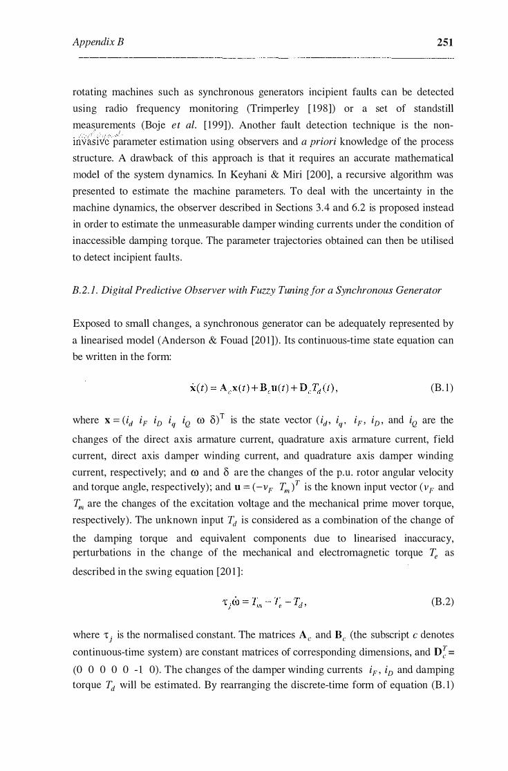
Appendix B 251
rotating machines such as synchronous generators incipient faults can be detected
using radio frequency monitoring (Trimperley [ 1 98]) or a set of standstill
measurements (Boje et al. [ 199]) . Another fault detection technique is the non-(/ //' > . ' / '
invasive parameter estimation using observers and a priori knowledge of the process
structure. A drawback of this approach is that it requires an accurate mathematical
model of the system dynamics. In Keyhani & Miri [200] , a recursive algorithm was
presented to estimate the machine parameters. To deal with the uncertainty in the
machine dynamics, the observer described in Sections 3.4 and 6.2 is proposed instead
in order to estimate the unmeasurable damper winding currents under the condition of
inaccessible damping torque. The parameter trajectories obtained can then be utilised
to detect incipient faults .
B.2. 1 . Digital Predictive Observer with Fuzzy Tuning for a Synchronous Generator
Exposed to small changes, a synchronous generator can be adequately represented by
a linearised model (Anderson & Fouad [20 1]) . Its continuous-time state equation can
be written in the form:
(B. l )
where x == (id iF iv iq iQ ffi 8)T is the state vector ( id , iq , iF , iv , and iQ are the
changes of the direct axis armature current, quadrature axis armature current, field
current, direct axis damper winding current, and quadrature axis damper winding
current, respectively; and co and 8 are the changes of the p.u. rotor angular velocity and torque angle, respectively) ; and u == (-vF Tm l is the known input vector (vF and
Tm are the changes of the excitation voltage and the mechanical prime mover torque,
respectively) . The unknown input 1d is considered as a combination of the change of
the damping torque and equivalent components due to linearised inaccuracy, perturbations in the change of the mechanical and electromagnetic torque � as
described in the swing equation [20 1 ] :
(B .2)
where 't 1 is the normalised constant. The matrices Ac and Be (the subscript c denotes
continuous-time system) are constant matrices of corresponding dimensions, and D�'=
(0 0 0 0 0 - 1 0) . The changes of the damper winding currents iF , iv and damping
torque Td will be estimated. By rearranging the discrete-time form of equation (B . 1 )

Appendix B 252
into the form of equation (3 .7 1 ) with x 1 = ( id iF iq co 3l and x2 = (iD iQ l , and
augmenting it with the approximation
(B .3)
the partitioned form of equation (3 .75) can be obtained. By choosing the observer (0 0 ll l2 0
J ( ) gain L1 = and L2 = 0 0 !5 !6 0 , the observer equation is 0 0 !3 l4 0 written as :
zi (k + 1) = filz1 (k) + ,h2z2 (k) + .!;3 w(k) + gi l id (k) + gi 2iF (k) + gi3iq (k) + gi4co(k) +
+ gi 53(k) - hi lvF (k) + hi 2Tm (k), i = 1, 2
w(k + 1 ) = f31z1 (k) + f12z2 (k) + f33w(k) + g31 id (k) + g32iF (k) + g33iq (k) + g34co(k) + A
+ g353(k) - h31vF (k) + h32Tm (k) - ii'd(k - 1)
A
iQ (k) = z2 (k) + l3iq (k) + l4co(k ) ,
A
Td (k) = w(k) + l5iq (k) + l6co(k), (B .4)
where z1 (k), z2 (k) and w(k) are the observer states, .!;1 , giJ , and hiJ are coefficients
calculated from equation (3 .76b) . For a given coefficient y = y0 , a solution for the
observer deadbeat condition can be obtained as follows:
(B .5)

Appendix B 253
where the matrix elements aiJ , di (i, j = 1 , 2, . . . , 5) found in the form (3.75) of the
system discrete-time state equation.
Taking into account uncertainties in the mathematical model of a generator, the
observer predictive coefficient y in equation (B .3) will be tuned, using the fuzzy logic
approach as described in Section 6.2. The following membership functions are assigned to y and the rate of change r( k) of the unknown input Td ( k ) :
{1 , "f = Y m 1-l ( y _large)=
O, Y ::f Ym
{1 , y = 0 !-1 ( y _small)= ,
0, y :t 0
!-11 (r _small)=e -crl rl ,
(B .6)
where y m ' cr are some positive constants . By inference and using equation (6.3), the
predictive coefficient y can be expressed in an explicit form as y = y me-alrl .
B.2.2. Ident�fication of Machine Parameters
A A
Once the estimates of the unmeasurable states iD (k) , iQ (k) and the unknown input A
Td (k) are obtained, the identification problem is the determination of the discrete-
time state matrices of the form (6. 1 ) and then, matrices of the generator state equation
(B . l ). The least squares identification algorithm (Sinha & Kwong [202] , Kreisselmeier [203]) is used. Denoting X = (id iF iD iq
iQ co ol and
U = ( -vF ( Tm - Td )l , and following the simplified version of the generalised least
square algorithm described in Keyhani & Miri [200], we can find the estimates A and A
B of matrices A and B in the state equation
X(k + l) = AX(k) + BU(k) . (B.7)

Appendix B 254
A
Note that matrix D is omitted in equation (B .7) by the use of 1�1 - Td as the prime A
torque. If there exists a nonsingular matrix Q to diagonalise A or put it into Jordan
form A = Q-1AQ , then matrices Ac and Be of the continuous-time sate equation
corresponding to Equation ( 1 8) can be determined as :
(B .8)
where Ac (ii) = _!_ ln A( ii) , i= 1 ,2, . . . ,7 . T
A
The estimates of the generator damping constant Dw (k) and parameter matrices M
and K (Anderson & Fouad [201]) can then be found as :
A
Dw (k) = �(�;, M = -(BcTb )-1 , K = B�1Ac , (B.9)
(0 1 0 0 0 0 0) where Tb = , and M and K have the following forms, using the
0 0 0 0 0 1 0
notation described in Anderson & Fouad [20 1 ] :
Lctr. kMp kMv 0 0 0 0
kMF Lp MR 0 0 0 0
kMv MR Lv 0 0 0 0
M = 0 0 0 Lqr. kMQ - 'Aqo 0
0 0 0 kMQ LQ 0 0
0 0 0 0 0 - 't . .I 0
0 0 0 0 0 0 1
Rr, 0 0 m o Lqr. 0 rp 0 0
0 0 rv 0
K = -moLctr, - ro0kMp - m0kMv Rr. 0 0 0 0
'Aqo - Ld iqo -kMpiqo -kMviqo -'Ado + Lqido 3 3 3 3
0 0 0 0
m0kMQ 0
0
0
rQ kMQiqo
3 0
lvqOL- - K cos(o0 - a)
0 0
0 0
- 'Ado'£ - K sin(o0 - a)
0 0
0 0
- 1 0
(B . I 0)

Appendix B 255
The parameter estimates obtained can be used to trace a trajectory for each parameter
of the machine as its operating conditions are changing. By comparing the trajectory
for a given parameter with earlier trajectories , any deterioration which may cause
changes in this parameter can be detected. Possible faults due to temperature rise can A A
also be detected from the estimates of damper winding currents i D ( k ) , iQ ( k) and
resistances rD , rQ by calculating Joule terms ri2
.
B.3 Illustrative example
Simulation results are provided to detect of damper winding currents and the damping
coefficient of a synchronous machine taking into account its load variations (values of
the machine parameters are taken from Example 6.2 in Anderson & Fouad [201]) .
With the sampling period T = O.Olsec, the actual and estimated damping torque and damper winding currents are shown in Figure B. 1 and Figure B .2 when Tm= l , vp= l , and the damping torque i s assumed to be Td (k) = 5 x 1 0-4 k at the system nominal
parameters .
The identification error is estimated by
(B . l l )
A A
where Ac,iJ and Ac,ij are the i-th row andj-th column elements of the matrices Ac and
Ac . This error e(k) is less than 0. 1 % after 50 sampling periods. Note that as stated in
Boje et al. discussion of [ 1 99], the identification error is sensitive to the initial values
of the least squares algorithm.
Figure B .3 depicts the actual (curve 1) and estimated damping torques with fuzzy
tuning y = 0. 5e -Zirl (curve 2) and without fuzzy tuning y = 0 (curve 3) when the total
armature resistance is increased 200% (R'L = 3Rr.. ,nom) and the damping torque varies
sinusoidally Td = 0. 5 ( 1 - sin t) p.u.
The results obtained indicates that the digital predictive observer with fuzzy tuning is
less sensitive to system parameter variations (in this case, the load changes of the synchronous machine Re ) . Thus, the identification process is made more robust.
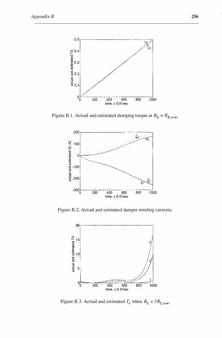
Appendix B
� 0.4
400 600 800 1 000 time. x 0.01 sec
Figure B . 1. Actual and estimated damping torque at Rr, = R'L nom.
200 ,---�----�----�----�---.
Q 1 00 0 "'0 <ll n; E � <ll -g -1 00 !tl ro ::1 � -200
-300 c__ _ _. __ ___,_ ___ .J._ __ --:"-::----' 0 200 400 600 800 1 000
time. x 0 . 0 1 sec
Figure B .2 . Actual and estimated damper winding currents.
20 .---�----�----�----�----.
"'0 l- 1 5 "'0 <ll iii .5 � 1 0 "'0 c: !tl ro � 5 !tl
time. x 0 . 0 1 sec
Figure B .3 . Actual and estimated Td when R"l:. = 3R"l:. nom ·
256

Appendix B 257
B.4 Conclusion
A digital predictive observer with fuzzy tuning has been proposed to estimate the
damping torque and damper winding currents of a synchronous machine. The
advantage of this observer is that it can provide correct estimates of not only the
unmeasurable states but also the unknown inputs to the system. Furthermore, with
simple tuning schemes the observer is made more robust against any deviation of
system parameters. The information about the inaccessible damper winding currents
and damping torque is then utilised to identify the continuous-time state matrix of the
machine linearised model using a generalised least quare recursive algorithm. The
parameter trajectories obtained enable the possibility of detecting incipient faults of a
synchronous machine.

References
[ I ] F. Harashima, "Power electronics and motion control - a future perspective,"
Proceedings of the IEEE, Vol. 82, No. 8, pp. 1 107- 1 1 10, August 1994.
[2] P. Dorato, "A historical review of robust control, " IEEE Control System
Magazine, Vol . 7, pp. 44-47, April 1 987.
[3] P. Dorato, R. Tempo, and G. Muscato, "Bibliography on robust control ,"
Automatica, Vol. 29, No. 1 , pp. 201 -2 13, January 1993.
[4] Y. Tsypkin, "New approaches to control theory," Vestnik RAN, No. 3 , pp. 1 12-
1 1 5, March 1992. (In Russian).
[5] V. A. Kharitonov, "On the asymptotic stability of the equilibrium point of a
family of linear differential equation systems, " Differential Equations, Vol.
14, No. 1 1 , pp. 2086-2088, November 1978. (In Russian).
[6] H. Kwakernaak, "Robust control and Hoo -optimisation - tutorial paper, "
Automatica, Vol. 29, No. 2, pp. 255-273, February 1 993.
[7] S . Y. Emelyanov, Variable structure control systems, Moscow: Nauka, 1 967.
(In Russian) .
[8] V. Utkin, Sliding modes and their application in variable structure systems,
Moscow: Nauka, 1 974. (In Russian) .
[9] Q. P. Ha, Design and investigation of a robust modal control system for
electric drives of positioning mechanisms, PhD Thesis , Moscow Power
Engineering Institute (MEl), December 1992. (In Russian).
[ 1 0] V. K. Kumar and N. Mani, "The application of artificial intelligence
techniques for intelligent control of dynamical physical systems,"
International Journal of Adaptive Control and Signal Processing, Vol. 8 , pp.
379-392, August 1 994.

References 259
[ 1 1 ] B . K. Bose, "Expert system, fuzzy logic, and neural network applications in
power electronics and motion control," Proceedings of the IEEE, Vol . 82, No.
8, pp. 1 303- 1 323, August 1994.
[ 1 2] L. A. Zadeh, "Fuzzy sets, " Inform. Control, Vol. 8, pp. 338-353, 1965.
[ 1 3 ] S . S . L. Chang and L. A. Zadeh, "Fuzzy mapping and control," IEEE Trans.
Syst., Man, Cybern. , Vol. SCM-2, No. 1 , pp. 30-34, January 1972.
[ 1 4] D. G. Schwartz, G. J . Klir, H. W. Lewis III, and Y. Ezawa, "Application of
fuzzy sets and approximate reasoning, " Proceedings of the IEEE, Vol. 82, No.
4, pp. 482-498, April 1994.
[ 1 5] B. Widrow and M. A. Lehr, "30 years of adaptive neural networks: perceptron,
madaline and backpropagation," Proceedings of the IEEE, Vol. 78, No. 9, pp.
14 1 5- 1442, September 1 994.
[ 1 6] Q. P. Ha and M. Negnevitsky, "New trends in control theory and their
reflection in electrical engineering education, " Proceedings of the Pac{fic
Region Conference on Electrical Engineering Education (PRCEEE95),
Melbourne, Australia, pp. 109- 1 12, February 1 995.
[ 1 7] K. J. Astrom, C . C. Hang, P. Persson, and W. K. Ho, "Toward intelligent PID
control , " Automatica, Vol. 28, No. 1 , pp. 1 -9, January 1 992.
[ 1 8] A. A. Voda and I. D. Landau, "A method for the auto-calibration of PID
controllers, " Automatica, Vol. 3 1 , No. 1 , pp. 4 1 -53, January 1995.
[ 1 9] Q. P. Ha and V. G. Alferov, "Robust modal controller for position drives, "
Preprints of the Electrical Engineering Congress (EEC'94), Sydney,
Australia, pp. 609-6 14, November 1 994.
[20] H. C. Tseng and V. H. Hwang, "Servocontroller tuning with fuzzy logic , "
IEEE Trans. Contr. Syst. Technology, Vol. 1 , No. 4, pp. 262-269, December
1 993.
[2 1 ] Q. P . Ha and M. Negnevitsky, "Robust controllers with fuzzy tuning" ,
Australian Journal ofintelligent Information Processing Systems, Vol. 3, No.
3, pp. 33-40, 1 996.
[22] Q. P. Ha, M. Negnevitsky, and Z. Man, "Sliding mode control with fuzzy
tuning" , in Proceedings of the 4th IEEE Australian and New-Zealand
Conference on Intelligent Information Systems, Adelaide, Australia, pp. 2 1 6-
2 19, 1 996.

References 260
[23] D. T. Pham and L. Xing, Neural Networks for Identification, Prediction and
Control, London : Springer-Verlag, 1 995.
[24] D. Psaltis, A. Sideris, and A. A. Yamamura, "A multilayered neural network
controller," IEEE Control System Magazine, Vol. 8 , No. 2, pp. 17-2 1 , April
1988.
[25] P. J. Werbos, "Backpropagation through time: what it does and how to do it?,"
Proceedings of the IEEE, Vol. 78, No. 9, pp. 1550- 1 560, September 1 994.
[26] W. T. Miller, R. S . Sutton, and P. J. Werbos, Neural networks for control,
MIT Press, Cambridge, MA, 1990.
[27] K. S. Narenda and K. Parthasarathy, "Identification and control for dynamic
systems using neural networks, " IEEE Trans. Neural Networks, Vol . 1 , No. 1 ,
pp. 4-27, March 1990.
[28] K. J. Hunt and D. Sbarbaro, "Neural networks for non-linear internal model
control, " Proceedings of the lEE, Part D, Control Theory Appl. ,Vol. 138 , No.
5, pp. 43 1 -438 , May 1 99 1 .
[29] E. Colina-Morles and N. Mort, "Neural network-based adaptive control
design," Journal of Systems Engineering, Vol. 2, No. 1 , pp. 9- 1 4, January
1 993.
[30] G. A. Rovithakis and M. A. Christodoulou, "A robust direct adaptive
regulation architecture using dynamic neural network model, " Proceedings of
the Int. Conf on System, Man and Cybernetics, San Antonio, Texas, USA, pp.
1 1 10- 1 1 15 , October 1 994.
[3 1 ] J . T . Evans, J . B . Gomm, J . B . Williams, P. J . G. Lisboa, and Q . S . To, "A
practical application of neural modelling and predictive control," in G. F.
Page, J . B. Gomm, and J . B. Williams (Eds.) , Applications of Neural
Networks to Modelling and Control, Chapman & Hall, London, 1993 .
[32] T. H. Lee, W. K. Tan, and M. H. Ang, Jr. , "A neural network control system
with parallel adaptive enhancements applicable to nonlinear
servomechanisms," IEEE Trans. Ind. Electronics, Vol. 4 1 , No. 3 , pp. 269-277,
June 1 994.
[33] F. Palis, A. Buch, U. Ladra, R. Kurrich, Q. P. Ha, and M. Negnevitsky, "Fuzzy
and neurocontrol of drive systems with changing parameters and load" , in
Proceedings of the 2nd European Power Electronics Chapter Symposium on

References 261
Electric Drive Design and Applications (EPE'96), Nancy, France, pp. 1 83-
1 86, June 1996.
[34] Q. P. Ha and M. Negnevitsky, "Neural network application for the position
drive of a swinging load," in Proceedings of the lASTED International
Conference on Modelling, Simulation and Optimisation (MS0'96), Gold
Coast, Australia, May 1996.
[35] Q. P. Ha and M. Negnevitsky, "Root locus application for damping capability
estimation of multi-mass electromechanical systems," in Proceedings of the
IEEE 21st International Conference on Industrial Electronics, Control, and
Instrumentation (IECON'95), Orlando, USA, Vol. 1 , pp. 633-638, November
1 995.
[36] V. G. Alferov and Q. P. Ha, "DC-motor position drives with robust modal
control," Elektrichestvo, No. 9 , pp. 1 7-24, 1995. (In Russian) .
[37] Q. P. Ha and M. Negnevitsky, "Fuzzy tuning in motion control" , in R. A.
Adey, G. Rzevski, and A.K. Sunol (Eds.) , Applications of Artificial
Intelligence in Engineering, Computational Mechanics Publications,
Southampton, UK, 1996, 734p.
[38] Q. P. Ha, M. Negnevitsky, and F. Palis, "Cascade PI Controllers with Fuzzy
Tuning, " to appear in Proceedings of the IEEE International Conference on
Fuzzy Systems (FUZZ-IEEE'97), Barcelona, Spain, July 1997.
[39] Q. P. Ha, "A digital predictive observer with fuzzy tuning for multi-mass
electromechanical systems," in Proceedings of the Australian Universities
Power Engineering Conference (AUPEC'95), Perth, Australia, Vol. 3 , pp.
428-433, September 1 995.
[40] Q. P. Ha, "A dynamic feedforward controller with fuzzy tuning for
electromechanical systems," in Proceedings of the Australian Universities
Power Engineering Conference (AUPEC'95), Perth, Australia, Vol . 3 , pp.
422-427, September 1995.
[41 ] Q. P . Ha and M. Negnevitsky, " A robust modal controller with fuzzy tuning
for multi-mass electromechanical systems," in Proceedings of the IEEE 3rd
Australian and New Zealand Conference on Intelligent Information Systems
(ANZIIS-95), Perth, Australia, pp. 2 14-219, November 1 995.
[42] Q. P. Ha and M. Negnevitsky, "Fuzzy tuning in robust modal control , " in
Proceedings of the 1st International Discourse on Fuzzy Logic and the

References 262
Management of Complexity (FLAMOC'96), Sydney, Australia, Vol. 2, pp.
1 60-1 64, January 1 996.
[43] Q. P. Ha and M. Negnevitsky, "A digital predictive observer for incipient fault
detection," in Proceedings of the lEE 3rd International Conference on
Advances in Power System Control, Operation & Management (APSCOM-
95), HongKong, Vol. 1 , pp. 1 83- 1 88, November 1 995.
[44] Q. P. Ha and M. Negnevitsky, "Neural network-based controller for servo
drives," in Proceedings of the IEEE 22nd International Conference on
Industrial Electronics, Control, and Instrumentation (IECON'96), Taipei,
Taiwan, Vol . 2, pp. 904-909, August 1 996.
[45] Q. P. Ha, "A Neural Network-Based Controller for Multi-Mass
Electromechanical Systems," in Proceedings of the Australian Universities
Power Engineering Conference (AUPEC'96), Melbourne, Australia, Vol. 1 ,
pp. 3 1 -36, October 1 996.
[46] W. Gawronski, "A balanced LQG compensator for flexible structures , "
Automatica, Vol. 30, No. 10 , pp. 1 555- 1 564, October 1993.
[ 4 7] S. K. Lin, "Minimal linear combinations of the inertia parameters of a
manipulator," IEEE Trans. Robot. and Automat. , Vol. 1 1 , No. 3 , pp. 360-373 ,
June 1 995.
[48] V. B. Klepikov and V. A. Samarskii , "P;��li�rities of frequency response of
electromechanical systems with friction load," Elektromekhanika, No. 2, pp.
62-67, May 1 990. (In Russian).
[ 49] V. G. Alferov and Q. P. Ha, "Root locus evaluation of the dynamic properties
and the pair of dominant roots, " Soviet Electrical Engineering, No. 64, No. 6,
pp. 35-40, June 1993.
[50] R. Dhaouadi, K. Kubo, and M. Tobise, "Analysis and compensation of speed
drive systems with torsional loads," IEEE Trans. Ind. Appli. , Vol. 30, No. 3 ,
pp. 760-765, June 1 994.
[5 1 ] V . I. Kljuchev, "Development of the theory of electrical drives with flexible
mechanical links: status and perspective," Elektrichestvo, No. 7, pp. 28-32,
July 198 1 . (In Russian) .
[52] B. V. Ol'khovikov, D. A. Kaminskaya, and A. B. Rozenvaig, "Analysis of the
dynamics of a two-mass electrical drive system on the basis of the roots of the
References 263
characteristic equation," Elektromekhanika, No. 5, pp. 98- 102, May 1 984. (In
Russian).
[53] N. A. Zadorozhny and V. D. Zemljakov, "Estimating the damping properties
of an electrical drive with an elastic mechanical component and viscous
friction at the motor shaft, " Elektrichestvo, No. 4, pp. 70-72, April 1989. (In
Russian) .
[54] V. I. Kljuchev, Theory of electrical drives, Moscow: Energoatomizdat, 1 985 .
(In Russian) .
[55] Q. P. Ha, "Root locus method application for damping capability estimation of
multi-mass electromechanical systems," in Preprints of the CONTROL'95
Conference, Melbourne, Australia, Vol. 1 , pp. 255-259, October 1 995.
[56] R. D. Lorenz, T. A. Lipo, and D. W. Novotny, "Motion control with induction
motors," Proceedings of the IEEE, Vol. 82, No. 8 , pp. 12 15- 1240, August
1 994.
[57] S. Nomura, T. Murakami, and K. Ohnishi, "Vibration control of multiple mass
system by estimated reaction torque, " in Proceedings of the IEEE 21st
International Conference on Industrial Electronics, Control, and
Instrumentation (IECON'95), Orlando, USA, Vol. 2, pp. 109 1 - 1 095,
November 1995.
[58] M. Matsuoka, T. Murakami, and K. Ohnishi, "Vibration suppression and
disturbance rejection control of a flexible link arm," in Proceedings of the
IEEE 21st International Conference on Industrial Electronics, Control, and
Instrumentation (IECON'95), Orlando, USA, Vol. 2, pp. 1260- 1265,
November 1 995 .
[59] S . P. Strelkov, Introduction to theory of oscillations, Moscow: Nauka, 1 964.
(In Russian).
[60] B . C. Kuo, Automatic control systems, Englewood Cliffs, NJ. : Prentice Hall ,
Inc. , 1 987.
[6 1 ] B . R . Barmish and R . Tempo, "The robust root locus," Automatica, Vol. 26,
No. 2 , pp. 283-292, February 1 990.
[62] Y. Tong and N. K. Sinha, "A computational technique for the robust root
locus," IEEE Trans. Ind. Electronics, Vol. 4 1 , No. 1 , pp. 79-85, February
1 994.

References 264
[63] B. Armstrong-Helouvry, P. Dupont, and C. Canudas de Wit, "A survey of
models, analysis tools and compensation methods for the control of machines
with friction," A utomatica, Vol. 30, No. 7, pp. 1 083-1 138 , July 1994.
[64] Y. Hori, H. Iseki, and K. Sugiura, "Basic consideration of vibration
suppression and disturbance rejection control of multi-inertia system using
SFLAC (State Feedback and Load Acceleration Control) , " IEEE Trans. Ind.
Appli. , Vol. 30, No. 4 , pp. 889-896, August 1994.
[65] Y. Dote, "Application of modern control techniques to motor control, "
Proceedings of the IEEE, Vol. 76, No. 4, pp. 438-454, April 1988.
[66] F. N. Bailey and C. H. Hui, "Loop gain-phase shaping for single-input-single-
output robust controllers , " IEEE Contr. Syst. Mag. , Vol. 1 1 , No. 1 , pp. 93- 1 0 1 ,
January 1 99 1 .
[67] J. V. De Vegte, Feedback control systems, Englewood Cliffs , NJ. : PrenticeHall, Inc. , 1 990.
[68] B. D. 0. Anderson and J. B. Moore, Optimal control: linear quadratic
method, Englewood Cliffs, NJ. : Prentice-Hall, Inc. , 1 990.
[69] K. J . Astrom, " Adaptive feedback control, " Proceedings of the IEEE, Vol. 75 ,
No. 2, pp. 1 85-2 10, February 1 987.
[70] R. A. DeCarlo , S . H. Zak, and G. P. Matthews, "Variable structure control of
nonlinear multivariable systems: a tutorial , " Proceedings of the IEEE, Vol. 76,
No. 3 , pp. 2 12-232, March 1 988 .
[7 1 ] K . Furuta, "VSS type self-tuning control," IEEE Trans. Ind. Electronics, Vol.
40, No. 1 , pp. 37-44, February 1993.
[72] N. T. Kuzovkov, Modal control and observers, Moscow: Mashinostroenje,
1 976. (In Russian).
[73] V. G. Alferov and Q. P. Ha, "A digital predictive observer, "
Elektromekhanika, No. 3 , pp. 7 1 -76, March 1992. (In Russian) .
[74] V. G. Alferov, Q. P. Ha, and R. M. Khusainov, "Drive control systems using a
disturbance observer, " in N. F. Ilynsky (Ed.), Industrial applications of
electric drives on the perspective element base, Moscow, pp. 93-99, May
1 992. (In Russian) .
[75] V. G. Alferov and Q. P. Ha, "Design of a modal control system for servo
drive, " Elektrichestvo, No. 6, pp. 48-54, June 1993. (In Russian) .

References 265
[76] T. M. Jahns, "Motion control with permanent-magnet AC machines,"
Proceedings of the IEEE, Vol. 82, No. 8, pp. 124 1 - 1 252, August 1 994.
[77] I. Boldea and S . A. Nasar, Vector control of AC drives, Boca Raton, Florida:
CRC Press, Inc . , 1992.
[78] J . S . Ko, J . H. Lee, S . K. Chung, and M. J. Youn, "A robust digital position
control of brushless DC motor with deadbeat load torque observer," IEEE
Trans. Ind. Electronics, Vol. 40, No. 1 , pp. 44-49, February 1 993 .
[79] Y. Y. Tzou and H. J. Wu, "Multi-microprocessor based robust control of an
AC induction servo motor, " IEEE Trans. Ind. Appli. , Vol. 26, No. 3, pp. 441 -
449, June 1990.
[80] R. E. Kalman, "On the general theory of control systems, " in Proceedings of
the First International Congress IFAC, Moscow, 1 960. Automatica and
Remote Control. London: Butterworth & Co. , Ltd. , Vol. 1 , pp. 48 1 -492, 1 96 1 .
[8 1 ] V . M. Terekhov, Discrete and continuous-time control systems in electrical
drives, Moscow: Power Engineering Institute (MEl), 1989. (In Russian).
[82] J. W. Umland and M. Safiudin, "Magnitude and symmetric criterion for the
design of linear control systems: What is it and how does it compare with the
others? ," IEEE Trans. Ind. Appli. , Vol. 26, No. 3, pp. 489-497, June 1 990.
[83] B . C. Kuo, Digital control systems, Holt, Rinehart and Winston, Inc. , 1 980.
[84] K. Ogata, Discrete-time control systems, Englewood Cliffs, NJ. : Prentice-Hall,
Inc. , 1 995.
[85] Y. Stepanenko, "Modal control of fast large-scale robot motions , " Trans. of
the ASME- Journal of Dynamic Systems, Measurement and Control, Vol. 109,
pp. 80-87, June 1987.
[86] J . Lu, J. S. Thorp, and H. D. Chiang, "Modal control of large flexible space
structures using collocated actuators and sensors, " IEEE Trans. Automat.
Contr. , Vol. 37, No. 1 , pp. 143-148, January 1 992.
[87] Y. A. Bortsov, N. D. Poljakhov, and V. V. Putov, Electromechanical systems
with adaptive and modal control, Leningrad: Energoatomizdat, 1 984. (In
Russian) .
[88] N. V. Kukharenko, "Modal control for DC electrical drives," Elektrichestvo,
No. 3 , pp. 48-53, March 1 990. (In Russian) .

References 266
[89] J . C. Doyle, B. A Francis, and A. R. Tannenbaum, Feedback control theory,
Maxwell MacMillan, NY: MacMillan, Inc. , 1 992.
[90] B . Wu, G. R. S iemon, and S . B. Dewan, "Eigenvalue sensitivity analysis of
GTO-CSI induction machine drives , " IEEE Trans. Ind. Appli. , Vol. 30, No. 3 ,
pp. 767-775, June 1 994.
[9 1 ] Q . P . Ha and V. G . Alferov, "On the problem of parameter sensitivity i n
control system of DC motor position drive, " Elektrichestvo, No. 1 , pp. 47-53,
January 1 996. (In Russian) .
[92] D. G. Luenberger, "An introduction to observers, " IEEE Trans. Automat.
Contr. , Vol. 16 , No. 6, pp. 596-662, December 1 97 1 .
[93] J . S. Meditch and G. H. Hostetter, "Observers for systems with unknown and
inaccessible inputs , " International Journal of Control, Vol. 19, No. 3, pp.
473-480, 1 974.
[94] P. Kudva, N. Viswanadham, and A Ramakrishna, "Observers for linear
systems with unknown inputs, " IEEE Trans. Automat. Contr. , Vol. 25 , No. 1 ,
pp. 1 1 3- 1 1 5, February 1980.
[95] F. Yang and R. W. Wilde, "Observers for linear systems with unknown
inputs, " IEEE Trans. Automat. Contr. , Vol. 33, No. 7, pp. 677-78 1 , July 1 988 .
[96] Y. Guan and M . Saif, "A novel approach to the design of unknown input
observers, " IEEE Trans. Automat. Contr. , Vol. 36, No. 5, pp. 632-635, May
1 99 1 .
[97] Y. Park and J . L. Stein, "Closed-loop, state and inputs observer for system
with unknown inputs, " International Journal of Control, Vol. 48, No. 3 , pp.
1 1 2 1 - 1 136, 1988 .
[98] M. Hou and P. C. Muller, "Design of observers for linear systems with
unknown inputs, " IEEE Trans. Automat. Contr. , Vol. 37, No. 6, pp. 871 -875,
June 1 992.
[99] K. Ohishi, M. Nakao, K. Ohnishi, and K. Miyachi, "Microprocessor
controlled DC motor for load insensitive servo system," IEEE Trans. Ind.
Electronics, Vol. 34, No. 1 , pp. 44-49, February 1987.
[1 00] P. B. Schmidt and R. D. Lorenz, "Design principles and implementation of
acceleration feedback to improve performance of DC drives, " IEEE Trans.
Ind. Appli. , Vol. 28, No. 3 , pp. 594-599, June 1992.

References 267
[ 1 0 1 ] F. J. Chang, H . J. Liao, and S . Chang, "Position control of DC motors via
variable structure systems: a chattering alleviation approach, " IEEE Trans.
Ind. Electronics, Vol. 37, No. 6, pp. 452-459, December 1990.
[1 02] T. Egami, H. Morita, and T. Tsuchiya, "Efficiency-optimised model reference
adaptive control system for a DC motor," IEEE Trans. Ind. Electronics, Vol.
37, No. 1 , pp. 28-33 , February 1990.
[1 03] F. Jabbari and W. E . Schmitendorf, "A noniterative method for the design of
robust linear controllers, " IEEE Trans. Automat. Contr. , Vol. 35, No. 8, pp.
954-957, August 1 990.
[ 1 04] W. C. Yang and M. Tomizuka, "Discrete-time Robust Control via state
feedback for single input systems, " IEEE Trans. Automat. Contr. , Vol. 35, No.
5, pp. 590-598, May 1 990.
[1 05] T. S. Perry, "Lotfi A. Zadeh," IEEE Spectrum, pp. 32-35, June 1995 .
[ 1 06] L. A. Zadeh, Industrial applications of fuzzy control, M. Sugeno, Ed.
Amstterdam: North Holland, 1 985.
[ 1 07] L. A. Zadeh, "Outline of a new approach to the analysis of complex systems
and decision processes, " IEEE Trans. Syst., Man, Cybern. , Vol. SCM-3, No.
1 , pp. 28-44, January 1 973 .
[ 108] L. A. Zadeh, " Computing with words - a paradigm shift," in Proceedings of
the 1st International Discourse on Fuzzy Logic and the Management of
Complexity (FLAMOC'96), Sydney, Australia, Vol . 1 , pp. 3- 10, January 1 996.
[1 09] E. H. Mamdani , "Application of fuzzy algorithms for control of a simple
dynamic plant, " Proc. of the lEE, Vol. 1 2 1 , No. 1 2, pp. 1 585- 1 588, 1 974.
[ 1 1 0] C. C. Lee, "Fuzzy logic in control systems: fuzzy logic controller- Part I & II,"
IEEE Trans. Syst. , Man, Cybern. , Vol. SCM-20, No. 1 , pp. 404-435, March
1 990.
[ 1 1 1 ] T. T. Truong and W. Hofmann, "A new sp]i)ed controller with fuzzy tuning,"
in Proceedings of the IEEE 21st International Conference on Industrial
Electronics, Control, and Instrumentation (IECON'95), Orlando, USA, Vol. 2,
pp. 1 484- 1489, November 1 995 .
[ 1 1 2] Q. P. Ha, "PI controllers with fuzzy tuning," lEE Electronics Letters, VoL 32,
No. 1 1 , pp. 1 043- 1 044, May 1996.

References 268
[ 1 1 3] R. Jager, "Fuzzy logic in control," Ph.D. thesis, Technische Universiteit Delft,
1 995.
[ 1 1 4] J. M. Mendel, "Fuzzy logic systems for engineering: a tutorial , " Proceedings
ofthe IEEE, Vol. 83 , No. 3, pp. 345-377, March 1 995.
[ 1 1 5] R. R. Yager and D. P. Filev, "Template-based fuzzy systems modeling, " J.
lntell. and Fuzzy Syst. , Vol. 2, pp. 39-54, 1 994.
[ 1 1 6] L. A. Zadeh, "The concept of a linguistic variable and its application to
approximate reasoning, " Inf Sciences, Vol. 8, pp. 1 99-249, 1 975.
[ 1 17] E. Cox, The fuzzy systems handbook, Cambridge, MA: AP Professional, 1 994.
[ 1 1 8] H.-J. Zimmermann, Fuzzy set theory and its applications, Norwell , MA:
Kluwer Academic Publishers, 1 985.
[ 1 1 9] B . Kosko, Neural networks andfuzzy systems: a dynamical systems approach
to machine intelligence, Englewood Cliffs, NJ: Prentice-Hall, 1 992.
[ 1 20] D. Dubois and H. Prade, "Fuzzy logic and the generalised modus ponens
revisited," Cybern. Syst. , Vol. 1 5, No. 1 , pp. 3-4, 1 984.
[ 1 2 1 ] P. M. Larsen, "Industrial applications of fuzzy logic control, " Int. J. Man,
Mach. Studies, Vol. 1 2, No. 1 , pp. 3 - 10, 1 980.
[ 1 22] L. A. Zadeh, "The rationale for fuzzy control, " J. Dynamic Syst. Meas. Contr. ,
pp. 3-4, 1 972.
[ 1 23] M. Sugeno and M. Nashida, "Fuzzy control of a model car," Fuzzy Sets Syst. ,
Vol. 1 6, pp. 1 03- 1 1 3 , 1 985 .
[ 1 24] S . G. Cao, N. W. Rees, and G. Feng, "Stability analysis of fuzzy control
systems," in Proceedings of the IEEE 2nd Australian and New Zealand
Conference on Intelligent Information Systems (ANZIIS-94), Brisbane,
Australia, pp. 2 19-223, November 1 994.
[ 1 25] T. Procyk and E. H. Mamdani, "A linguistic self-organising process
controller, " Automatica, Vol. 1 5, No. 1 , pp. 1 5-30, 1 979.
[ 1 26] S. Shao, "Fuzzy self-organising controller and its application for dynamic
processes," Fuzzy Sets Syst. , Vol. 26, pp. 1 5 1 - 1 64, 1 988 .
[ 1 27] W. A. Kwong, K. M . Passino, E . G. Laukonen, and S . Yurkovich, "Expert
supervision of fuzzy learning systems for fault tolerant aircraft control, "
Proceedings of the IEEE, Vol. 83 , No. 3, pp. 466-482, March 1 995.

References 269
[ 1 28] J.-S. R. Jang and C.-T. Sun, "Neuro-fuzzy modelling and control, "
Proceedings of the IEEE, Vol. 83, No. 3, pp. 378-406, March 1 995.
[ 1 29] E. H. Mamdani and S. Assilian, "An experiment in linguistic synthesis with a
fuzzy logic controller," Int. J. Man Machine Studies, Vol. 7 , No. 1 , pp. 1 - 1 3 ,
1 975.
[ 1 30] R. R. Yager and D. P. Filev, Essentials offuzzy modeling and control, NY: John Wiley & Sons, Inc. , 1 994.
[ 1 3 1 ] L. I. Larkin, "A fuzzy logic controller for aircraft flight control" , i n Industrial
Applications of Fuzzy Control, M. Sugeno (Ed.), Amsterdam: North Holland,
87- 104, 1 985.
[ 1 32] H. Hellendoorn and C. Thomas, "Defuzzification in fuzzy controllers, " J.
Intel!. Syst. , Vol. 1 , pp. 1 09- 1 23 , 1993.
[ 1 33] J.-S. R. Jang and N. Gulley, Fuzzy logic toolbox for use with MATLAB,
Natick, MA: The Math Works, Inc. , 1995.
[ 1 34] Negnevitsky, M. , Ha, Q.P. , L.P. Chee, and T.H. Ting, "A Fuzzy Logic
Controller for an overhead crane," in Proceedings of the 1st International
Discourse on Fuzzy Logic and the Management of Complexity (FLAMOC'96),
Sydney, Australia, Vol. 2, pp. 17 1 - 175, January 1996.
[ 1 35] Fuzzy Inference Development Environment FIDE, Ver. 2.0, User's Manual,
Aptronix, 1 994.
[ 1 36] J. B. Kiszka, M. M. Gupta, and P. N. Nikiforuk, "Energetistic stability of
fuzzy dynamic systems, " IEEE Trans. Syst. , Man, Cybern. , Vol. SCM- 15 , No.
5, pp. 783-792, September 1 985.
[ 1 37] V. G. Moudgal, W. A. Kwong, K. V. Passino, and S . Yurkovich, "Fuzzy
learning control for a flexible-link robot," IEEE Trans. Fuzzy Syst. , Vol. 3 ,
No. 2, pp. 199-210, May 1 995.
[ 1 38] Y. M. Park, U . C. Moon, and K. Y. Lee, "A self-organising fuzzy logic
controller for dynamic systems using a fuzzy auto-regressive moving average
model ," IEEE Trans. Fuzzy Syst. , Vol. 3, No. l , pp. 75-82, February 1995.
[ 1 39] D. A. Linkens and H. 0. Nyongesa, "Genetic algorithms for fuzzy control -
Part 1&2," Proceedings of the lEE, Part D, Control Theory Appl. , Vol. 142,
No. 3 , pp. 1 6 1 - 1 85 , May 1 995.

References 270
[ 140] F. Palis, A. Buch, U. Ladra, R. Kurrich, Q. P. Ha, and M. Negnevitsky,
"Robust control using neuro-fuzzy approach" , in Proceedings of the
International Conference on Electrical Drives and Power Electronics
(EDPE'96), Kosice, Slovakia, Vol . 1 , pp. 1 94- 198 , October 1 996.
[ 14 1 ] D. McNeil and P . Freiberger, Fuzzy logic, NY: Simon & Schuster, 1 993 .
[ 142] C. Kessler, "Das symmetrische optimum" , Regelungstechnik, Vol. 6, pp. 395-
400, 1958.
[ 143] J. G. Ziegler and N. B. Nichols, "Optimum setting for automatic controllers" ,
Trans. of the ASME- Journal of Dynamic Systems, Measurement and Control,
Vol . 64, pp. 759-768, 1 948.
[ 144] C. C. Hang, K. J. Astrom, and W. K. Ho, "Refinements of the Ziegler-Nichols
tuning formula" , Proceedings of the lEE, Part D, Control Theory Appl. ,Vol .
1 38 , No. 2, pp. 1 1 1 - 1 1 8 , February 199 1 .
[ 1 45] K. J. Astrom and T. Hagglund, "Automatic tuning of simple regulators with
specification on phase and gain margin, " Automatica, Vol. 20, No. 5, pp. 645-
65 1 , May 1 984.
[ 146] Y. Dote, "Stability analysis of variable-structured PI controller by fuzzy logic
for servo systems" , in Proceedings of the 30th IEEE Conference on Decision
and Control CDC/9 1 , pp. 12 1 7- 12 1 8, Brighton, UK, 199 1 .
[ 1 47] A. Suyitno, J . Fujikawa, H. Kobayashi, and Y. Dote, "Variable-structured
robust controller by fuzzy logic for servomotors, " IEEE Trans. Ind.
Electronics, Vol. 40, No. 1 , pp. 80-87, February 1 993 .
[ 1 48] Q. P. Ha, "A robust sliding mode controller with fuzzy tuning, " lEE
Electronics Letters, Vol. 32, No. 17, pp. 1626- 1 628, August 1996.
[ 1 49] D. Graham and R. C. Lathrop, "The sythesis of 'optimum' transient response:
criteria and standard forms, " Trans. AlEE, Vol. 72, Part 2, pp. 273-288, 1 953.
[ 1 50] H. Ying, W. Siler, and J. J. Buckley, "Fuzzy control theory: A nonlinear case, "
Automatica, Vol. 26, No. 5, pp. 5 13-520, May 1 990.
[ 1 5 1 ] H . Ying, "The simplest fuzzy controllers using different inference methods are
different nonlinear proportional-integral controllers with variable gains,"
Automatica, Vol. 29, No. 6, pp. 1 597- 1 589, Jun 1 993.

References 271
[ 1 52] J . -J. E. Slotine and S . S . Sastry, "Tracking control of nonlinear systems using
sliding surface, with application to robot manipulators" , Int. J. Contr. , Vol. 38,
No. 2, pp. 465-492, 1 983 .
[ 1 53] S . K . Spurgeon , "Choice of discontinuous sliding mode control", Int. 1. Contr. , Vol. 53, No. 1 , pp. 1 6 1 - 179, 199 1.
[ 1 54] F. Zhou, and D. G. Fisher, "Continuous sliding mode control" , Int. J. Contr. ,
Vol. 55, No. 2, pp. 3 1 3-327, 1992.
[ 1 55] H. T. Nguyen and D. K. Nguyen, "Continuous sliding mode control" , in
Preprints of the Control 95, Melbourne, Australia, Vol. 1 , pp. 57-60, October
1995.
[ 1 56] Y. S . Lu and J. S. Chen, "A self-organising fuzzy sliding-mode controller
design for a class of nonlinear servo systems" , IEEE Trans. Ind. Electron. ,
Vol . 4 1 , No. 5 , pp. 492-502, October 1994.
[ 1 57] S. Y. Wang, C. M. Hong, C. C. Liu, and W. T. Yang, "Design of a static
reactive power compensator using fuzzy sliding mode control" , Int. J. Contr. ,
Vol. 63, No. 2, pp. 393-4 12, 1996.
[ 1 58] G. C. Hwang and S. C. Lin, "A stability approach to fuzzy control design for
nonlinear systems" , Fuzzy sets and systems, Vol. 48, pp. 279-287, 1 992.
[ 1 59] H. A. Malki, H. Li, and G. Chen, "New design and stability analysis of fuzzy
proportional-derivative control systems", IEEE Transactions on Fuzzy
Systems, Vol. 2, No. 4, pp. 245-254, Nov 1994.
[ 1 60] A. Hansson, B . Gruber, and J . Todli, "Fuzzy anti-reset PID controllers" , in
Preprints of the 12th IFAC Congress, Sydney, Australia, Vol . 10, pp. 389-392,
July 1 993.
[ 1 6 1 ] J. -J. E. Slotine and W. Li, Applied nonlinear control, Prentice Hall:
Englewood Cliffs, NJ, 1 990.
[ 1 62] T. Eisaka, Y. Zhong, S. Bai, and R. Tagawa, "Evaluation of robust model
matching for the control of a DC servo motor" , Int. J. Control, Vol 50, No.2,
pp. 479-493, 1 989.
[ 1 63] Q. P. Ha and F. Palis, "Fuzzy logic application in a robust modal controller for
position drives, " in Proceedings of the 30th Universities Power Engineering
Conference ( UPEC'95), London, UK, Vol. 1 , pp. 85-89, September 1995.
[ 1 64] ABB, Asea Brown Boveri Service Manual, January 1 984.

References 272
[ 1 65] F. Palis, A. Buch, U . Ladra, R. Kurrich, Q. P. Ha, and M. Negnevitsky,
"Robust control using neuro-fuzzy approach", in Proceedings of the
International Conference on Electrical Drives and Power Electronics (EDPE
96), Kosice, Slovakia, Vol. 1 , pp. 1 94- 198, October 1 996.
[ 1 66] L. 0. Hall and A. Kandel, "The evolution from expert systems to fuzzy expert
systems" , in Fuzzy Expert Systems, A. Kandel (Ed.), CRC Press, Inc. , 1 992.
[ 1 67] L. G. Kraft and D . P. Campagna, "Comparison between CMAC neural
network and two traditional adaptive control systems " , IEEE Contr. Syst.
Mag. , pp. 36-43 , Apri1 1 990.
[ 1 68] K. J. Hunt, D. Sbarbaro, R. Zbikowski, and P. J. Gawthrop, "Neural networks
for control systems- A survey, " Automatica, Vol. 28 , No. 6, pp. 1083- 1 1 12,
Jun 1992.
[ 1 69] T. Kohonen, Self-Organisation and Associative Memory, Springer-Verlag,
Berlin, 1 987.
[ 1 70] Y. H. Pao, Adaptive pattern recognition and neural networks, Addison
Wesley Publishing Company, Inc. , 1 989.
[ 1 7 1 ] D. E. Rumelhart, G. E. Hinton, and R. J. Williams, "Learning internal
representations by error propagation" , in D. E. Rumelhart and J. McClelland
(Eds.), Parallel Data Processing, Vol. 1 , M.I.T. Press , Cambridge, MA, 1 986.
[ 1 72] R. Zbikowski and P. J. Gawthrop, " A survey of neural networks for control" ,
in K . Warwick, G. W. Irwin, and K. J . Hunt (Eds.), Neural networks for
control and systems, Peter Peregrinus Ltd., London, UK, 1992.
[ 173] R. Krishnan, R. Monajemy, and N. Tripathi, "Neural control of high
performance drives : an application to the PM synchronous motor drive," in
Proceedings of the IEEE 21st International Conference on Industrial
Electronics, Control, and Instrumentation (IECON'95), Orlando, USA, Vol. 1 ,
pp. 38-43 , November 1 995 .
[ 1 74] G. S. Buja and F. Todesco, "Neural network implementation of a fuzzy logic
controller, " IEEE Trans. Ind. Electron., Vol. IE-4 1 , No. 6, pp. 663-665, 1 994.
[ 1 75] K. Yoshida and H. Kawabe, "A design of saturating control with a guaranteed
cost and its application to the crane control system," IEEE Trans. Automat.
Contr. , Vol. AC-37, No. 1 , pp. 1 2 1 - 1 27, 1992.

References 273
[1 76] R. Soussi and A.J. Koivo, "Adaptive control of cranes, " in Preprints of the
12th IFAC Congress, Sydney, Australia, Vol . 8 , pp. 237-240, July 1 993 .
[ 1 77] S . Chen, C.F.N. Cowan, and P.M. Grant, "Orthogonal least squares learning
algorithm for radial basis function networks, " IEEE Trans. Neur. Networks,
Vol. 2, No. 2, pp. 302-309, 1 99 1 .
[ 1 78] T. Poggio and F. Girosi, "Networks for approximation and learning, "
Proceedings of the IEEE, Vol. 78 , pp. 148 1 - 1497, 1990.
[1 79] M. Saad, P. B igras, L. A. Dessaint, and K. Al-Haddad, "Adaptive robot
control using neural networks" , IEEE Trans. Ind. Electron. , Vol . IE-41 , No. 2,
pp. 173-1 80, Apr 1 994.
[ 1 80] H. M. Tai, J. Wang, and K. Ashenayi, "A neural network-based tracking
control system" , IEEE Trans. Ind. Electron. , Vol. IE-39, No. 6, pp. 504-5 10 ,
Dec 1 992.
[ 1 8 1] S. K. Lin, "Minimal linear combinations of the inertia parameters of a
manipulator" , IEEE Trans. Robot. and Automat. , Vol. 1 1 , No. 3, 360 - 373 ,
1 995.
[ 1 82] T. H. Lee, C. C. Hang, L. L. Lian, and B. C. Lim, "An approach to inverse
non-linear control using neural networks" , Mechatronics, Vol. 2, No. 6, pp.
595 -61 1 , 1 992.
[ 1 83] Ch. Doschner and R. Schneider, "Bin neuronales Netz ftir das Erlernen der
Dynamik eines Roboters" , Pre prints of Otto-von-Guericke-Universitiit
Magdeburg, No 1 , 1 995.
[ 1 84] T. Kohonen, Self-organising Maps, Series in Information Sciences, Vol. 30,
Heidelberg: Springer-Verlag, 1 995.
[ 1 85] F. Palis and Th. Schmied, "Robust current and speed control of electrical
drives using fuzzy set theory", in Proc. of the International Conference on
Electrical Drives and Power Electronics, Kosice, Slovakia, Vol . 2, pp. 237-
242, 1 994.
[ 1 86] D. E. Van den Bout and T. K. Miller, III, "Graph partitioning using annealed
neural networks" , IEEE Trans. Neur. Networks, Vol. 1 , pp. 1 92-203 , 1 990.
[ 1 87] C. Peterson, "Parallel distributed approaches to combinatorial optimisation:
Benchmark on travelling salesman problem" , Neural Computation, Vol. 2, pp.
26 1 -269, 1 990.

References 274
[ 1 88] A. Cichocki and R. Unbehauen, Neural networks for optimization and signal
processing, B.G. Teubner Stuttgart, John Wiley & Sons Chichester: New
York, 1993 .
[ 1 89] C. Daoshen and B . K. Bose, "Expert system based automated selection of
industrial AC drives," in IEEE/IAS Annu. Meet. Conf Rec. , pp. 387-392,
1992.
[ 1 90] Q. P. Ha, M. Negnevitsky, and Z. Man, "Dominant pole-based controller for
maximal damping of multi-mass systems", to appear in Proceedings of the
2nd Asian Control Conference (ASCC-97), Seoul, Korea, July 1 997 .
[ 1 9 1 ] F Jabbari and W. E. Schrnitendorf, "Robust linear controllers using
observers, " IEEE Trans. Automat. Contr. , Vol. 36, No. 1 2, pp. 1 509- 1 5 14,
Dec 199 1 .
[ 192] Z. Man, X. Yu, and Q. P. Ha, "A study of uncertainty bound for rigid robot
control systems" , to appear in Proceedings of the 2nd Asian Control
Conference (ASCC 97), Seoul, Korea, July 1997 .
[ 1 93] D. E. Thomas and B. Armstrong-Helouvry, "Fuzzy logic control - Taxonomy
of demonstrated benefits, " Proceedings of the IEEE, Vol. 83, No. 3 , pp. 407-
42 1 , March 1 995.
[ 1 94] Q. P. Ha and M. Negnevitsky, "Continuous variable structure systems with
fuzzy tuning" , submitted to the IEEE 5th Australian and New Zealand
Conference on Intelligent Information Processing Systems (ANZIIS 97),
Dunedin, New-Zealand, November 1 997.
[ 1 95] Z. Man, X. Yu, and Q. P. Ha, "Adaptive control using fuzzy basis function
expansion for SISO linearisable nonlinear systems" , to appear in Proceedings
of the 2nd Asian Control Conference (ASCC 97), Seoul, Korea, July 1 997 .
[ 196] R. Isermann, "Fault diagnosis of machines via parameter estimation and
knowledge processing - tutorial paper" , Automatica, Vol. 29, No.4, pp. 8 1 5-
835, April 1 993 .
[ 1 97] P. M. Frank, "Fault diagnosis in dynamic systems using analytical and
knowledge-based redundancy - a survey and some new results" , Automatica,
Vol. 26, No. 3 , pp. 459-474, March 1 990.
[ 198] J. Trimperley, "Incipient fault detection through neutral RF monitoring of
large rotating machines," IEEE Trans. PAS, Vol . PAS- 102, No.3 , pp. 693-698,
1 983 .

References 275
[ 1 99] E. S. Boje, J. C. Balda, R. G. Harley, and R. C. Beck, "Time-domain
identification of synchronous machine parameters from simple standstill
tests, " IEEE Trans. Energy Conversion, Vol. EC-5, pp. l 64- 175, 1 990.
[200] A. Keyhani and S . M. Miri, "Observers for tracking of synchronous machine
parameters and detection of incipient faults," IEEE Trans. Energy Conversion,
Vol. EC- 1 , pp. 1 84- 1 90, 1986.
[20 1 ] P . M . Anderson and A. A. Fouad, Power system control and stability, Vol. I,
The IOWA State University Press, Ames, Iowa, USA, 1 977.
[202] N. K. Sinha and Y. H. Kwong, "Recursive estimation of the parameters of
linear multivariable systems" , Automatica, Vol. AC- 15, No. 3 , pp. 47 1 -475,
1 98 1 .
[203] G. Kreisselmeier, "Stabilized least-squares type adaptive identifiers," IEEE
Trans. Automt. Control, Vol. AC-35, No. 3, pp. 306-3 10, 1990.