Embed Size (px)
Citation preview
EidgenössischeTechnische HochschuleZürich
Ecole polytechnique fédérale de ZurichPolitecnico federale di ZurigoSwiss Federal Institute of Technology Zurich
Institute of Computational Sciences
Ivo F. Sbalzarini
On Protein Diffusion in theEndoplasmic Reticulum
A computational approach using particle simulations
Semester thesis at the
Institute of Computational Sciences
Principal Adviser: Prof. Dr. Petros Koumoutsakos, Computational Sciences
Co-Adviser: Prof. Dr. Ari Helenius, Institute of Biochemistry, ETHZ
July 2001

ii
iii
Abstract
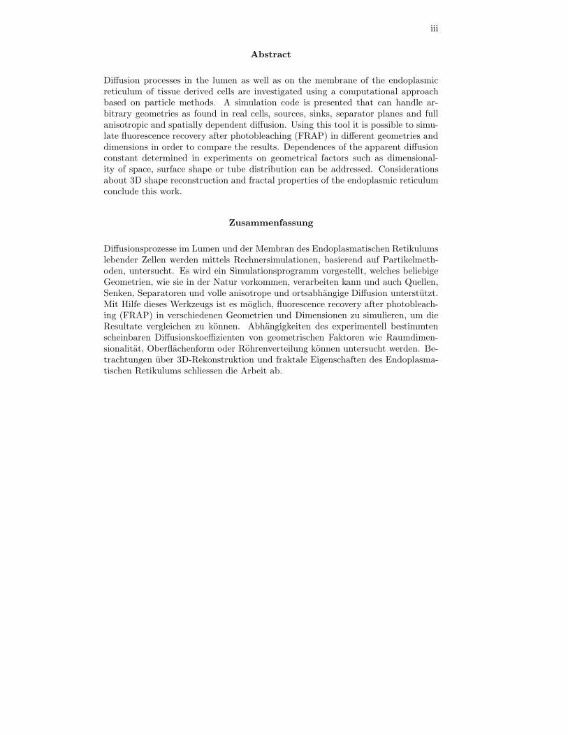
Diffusion processes in the lumen as well as on the membrane of the endoplasmicreticulum of tissue derived cells are investigated using a computational approachbased on particle methods. A simulation code is presented that can handle ar-bitrary geometries as found in real cells, sources, sinks, separator planes and fullanisotropic and spatially dependent diffusion. Using this tool it is possible to simu-late fluorescence recovery after photobleaching (FRAP) in different geometries anddimensions in order to compare the results. Dependences of the apparent diffusionconstant determined in experiments on geometrical factors such as dimensional-ity of space, surface shape or tube distribution can be addressed. Considerationsabout 3D shape reconstruction and fractal properties of the endoplasmic reticulumconclude this work.
Zusammenfassung
Diffusionsprozesse im Lumen und der Membran des Endoplasmatischen Retikulumslebender Zellen werden mittels Rechnersimulationen, basierend auf Partikelmeth-oden, untersucht. Es wird ein Simulationsprogramm vorgestellt, welches beliebigeGeometrien, wie sie in der Natur vorkommen, verarbeiten kann und auch Quellen,Senken, Separatoren und volle anisotrope und ortsabhangige Diffusion unterstutzt.Mit Hilfe dieses Werkzeugs ist es moglich, fluorescence recovery after photobleach-ing (FRAP) in verschiedenen Geometrien und Dimensionen zu simulieren, um dieResultate vergleichen zu konnen. Abhangigkeiten des experimentell bestimmtenscheinbaren Diffusionskoeffizienten von geometrischen Faktoren wie Raumdimen-sionalitat, Oberflachenform oder Rohrenverteilung konnen untersucht werden. Be-trachtungen uber 3D-Rekonstruktion und fraktale Eigenschaften des Endoplasma-tischen Retikulums schliessen die Arbeit ab.

iv
v
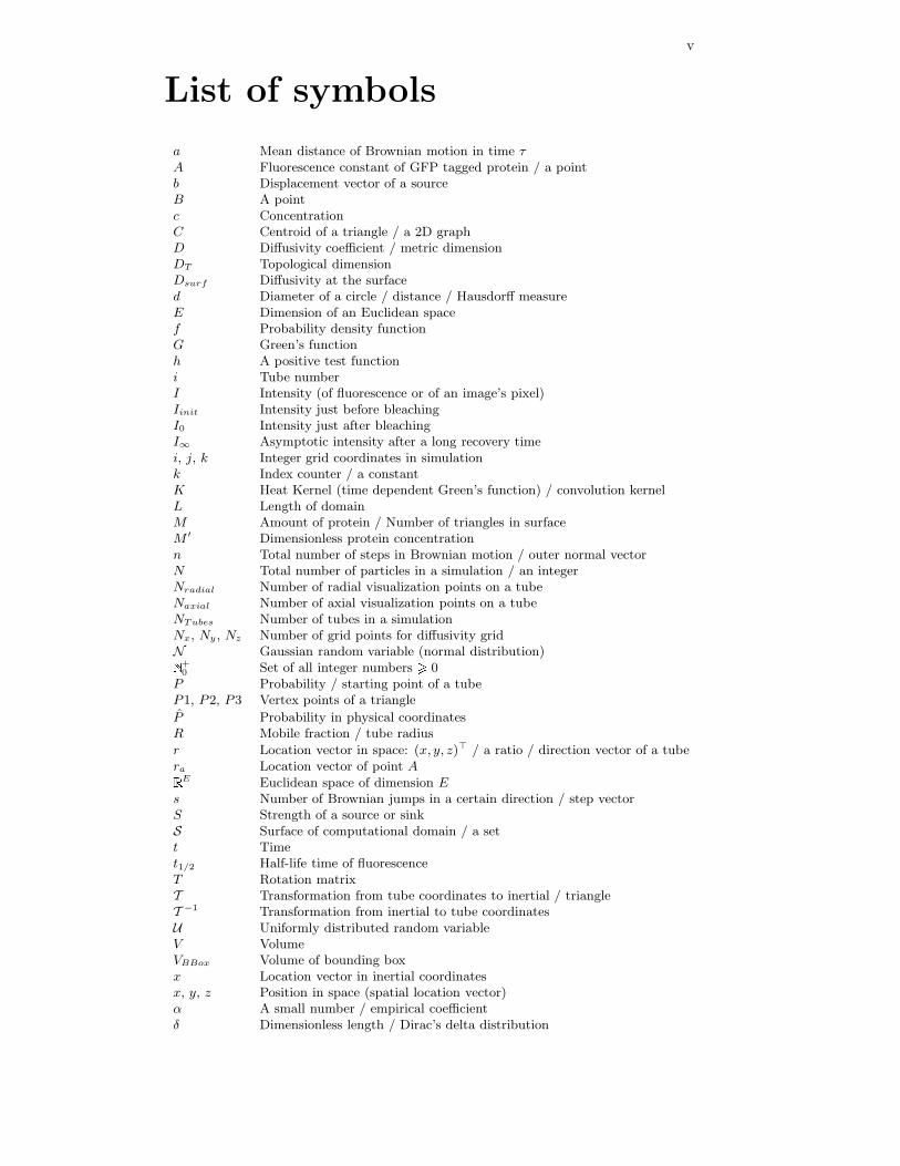
List of symbols
a Mean distance of Brownian motion in time τA Fluorescence constant of GFP tagged protein / a pointb Displacement vector of a sourceB A pointc ConcentrationC Centroid of a triangle / a 2D graphD Diffusivity coefficient / metric dimensionDT Topological dimensionDsurf Diffusivity at the surfaced Diameter of a circle / distance / Hausdorff measureE Dimension of an Euclidean spacef Probability density functionG Green’s functionh A positive test functioni Tube numberI Intensity (of fluorescence or of an image’s pixel)Iinit Intensity just before bleachingI0 Intensity just after bleachingI∞ Asymptotic intensity after a long recovery timei, j, k Integer grid coordinates in simulationk Index counter / a constantK Heat Kernel (time dependent Green’s function) / convolution kernelL Length of domainM Amount of protein / Number of triangles in surfaceM ′ Dimensionless protein concentrationn Total number of steps in Brownian motion / outer normal vectorN Total number of particles in a simulation / an integerNradial Number of radial visualization points on a tubeNaxial Number of axial visualization points on a tubeNTubes Number of tubes in a simulationNx, Ny , Nz Number of grid points for diffusivity gridN Gaussian random variable (normal distribution)
+0 Set of all integer numbers 0P Probability / starting point of a tubeP1, P2, P3 Vertex points of a triangle
P Probability in physical coordinatesR Mobile fraction / tube radius
r Location vector in space: (x, y, z) / a ratio / direction vector of a tubera Location vector of point A
E Euclidean space of dimension Es Number of Brownian jumps in a certain direction / step vectorS Strength of a source or sinkS Surface of computational domain / a sett Timet1/2 Half-life time of fluorescenceT Rotation matrixT Transformation from tube coordinates to inertial / triangleT −1 Transformation from inertial to tube coordinatesU Uniformly distributed random variableV VolumeVBBox Volume of bounding boxx Location vector in inertial coordinatesx, y, z Position in space (spatial location vector)α A small number / empirical coefficientδ Dimensionless length / Dirac’s delta distribution
vi
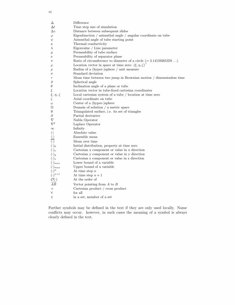
∆ Difference∆t Time step size of simulation∆z Distance between subsequent slidesϕ Eigenfunction / azimuthal angle / angular coordinate on tubeψ Azimuthal angle of tube starting pointκ Thermal conductivityλ Eigenvalue / Line parameterµ Permeability of tube surfaceν Permeability of separator planeπ Ratio of circumference to diameter of a circle (= 3.14159265359 . . .)ρ Location vector in space at time zero: (ξ, η, ζ)
ρ Radius of a (hyper-)sphere / unit measureσ Standard deviationτ Mean time between two jump in Brownian motion / dimensionless timeϑ Spherical angleθ Inclination angle of a plane or tubeξ Location vector in tube-fixed cartesian coordinatesξ, η, ζ Local cartesian system of a tube / location at time zeroζ Axial coordinate on tubeω Center of a (hyper-)sphereΩ Domain of solution / a metric spaceℵ Triangulated surface, i.e. its set of triangles∂ Partial derivative∇ Nabla Operator∇2 Laplace Operator∞ Infinity|·| Absolute value〈·〉 Ensemble mean
(·) Mean over time(·)0 Initial distribution, property at time zero(·)x Cartesian x component or value in x direction(·)y Cartesian y component or value in y direction(·)z Cartesian z component or value in z direction(·)min Lower bound of a variable(·)max Upper bound of a variable(·)n At time step n(·)n+1 At time step n+ 1O(·) At the order of−→AB Vector pointing from A to B× Cartesian product / cross product∀ for all∈ in a set, member of a set
Further symbols may be defined in the text if they are only used locally. Nameconflicts may occur. however, in such cases the meaning of a symbol is alwaysclearly defined in the text.
vii
Acronyms
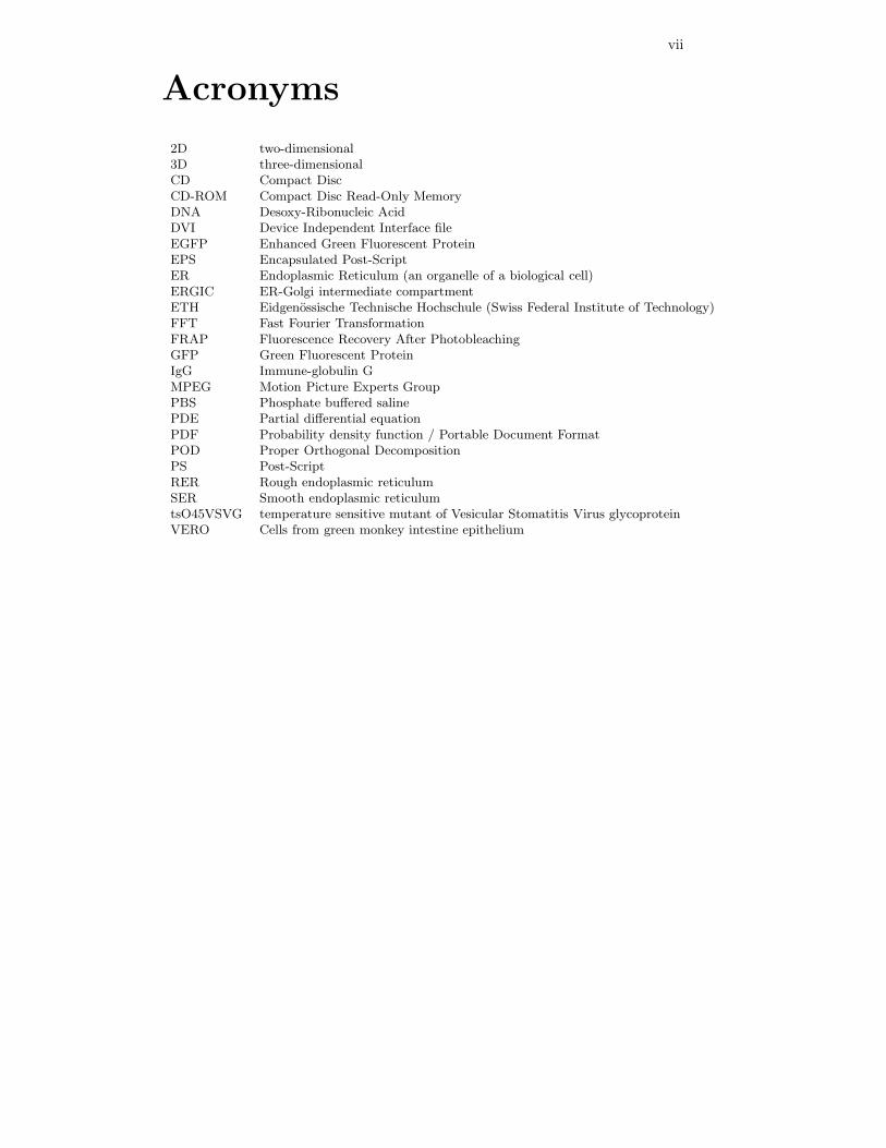
2D two-dimensional3D three-dimensionalCD Compact DiscCD-ROM Compact Disc Read-Only MemoryDNA Desoxy-Ribonucleic AcidDVI Device Independent Interface fileEGFP Enhanced Green Fluorescent ProteinEPS Encapsulated Post-ScriptER Endoplasmic Reticulum (an organelle of a biological cell)ERGIC ER-Golgi intermediate compartmentETH Eidgenossische Technische Hochschule (Swiss Federal Institute of Technology)FFT Fast Fourier TransformationFRAP Fluorescence Recovery After PhotobleachingGFP Green Fluorescent ProteinIgG Immune-globulin GMPEG Motion Picture Experts GroupPBS Phosphate buffered salinePDE Partial differential equationPDF Probability density function / Portable Document FormatPOD Proper Orthogonal DecompositionPS Post-ScriptRER Rough endoplasmic reticulumSER Smooth endoplasmic reticulumtsO45VSVG temperature sensitive mutant of Vesicular Stomatitis Virus glycoproteinVERO Cells from green monkey intestine epithelium

viii
Contents
1 Foreword 1
2 Introduction to the endoplasmic reticulum 3
3 The concept of FRAP analysis 73.1 The green fluorescent protein . . . . . . . . . . . . . . . . . . . . . . 73.2 FRAP analysis . . . . . . . . . . . . . . . . . . . . . . . . . . . . . . 113.3 Estimation of diffusivity . . . . . . . . . . . . . . . . . . . . . . . . . 12
3.3.1 Currently used models . . . . . . . . . . . . . . . . . . . . . . 133.4 Restatement of goals . . . . . . . . . . . . . . . . . . . . . . . . . . . 15
4 The simulation technique 174.1 On the relation of random walk and diffusion . . . . . . . . . . . . . 174.2 Simulation algorithm outline . . . . . . . . . . . . . . . . . . . . . . 214.3 Spatial dependence of D and anisotropy . . . . . . . . . . . . . . . . 224.4 3D code . . . . . . . . . . . . . . . . . . . . . . . . . . . . . . . . . . 224.5 2D code . . . . . . . . . . . . . . . . . . . . . . . . . . . . . . . . . . 244.6 Adding sources and sinks . . . . . . . . . . . . . . . . . . . . . . . . 244.7 Separator planes build compartments . . . . . . . . . . . . . . . . . . 254.8 Simulating FRAP analysis . . . . . . . . . . . . . . . . . . . . . . . . 25
5 FRAP analysis of 2D and 3D space diffusion 27
6 Surface diffusion on tubes 336.1 Description of tubes . . . . . . . . . . . . . . . . . . . . . . . . . . . 336.2 Coordinate transformations . . . . . . . . . . . . . . . . . . . . . . . 346.3 Surface diffusion . . . . . . . . . . . . . . . . . . . . . . . . . . . . . 376.4 Sources and sinks on tubes . . . . . . . . . . . . . . . . . . . . . . . 376.5 FRAP analysis at different angles . . . . . . . . . . . . . . . . . . . . 38
7 Combining surface and space diffusion 41
8 Diffusion on multiple tubes 43
9 Towards a more realistic domain geometry 479.1 Using triangulated domains . . . . . . . . . . . . . . . . . . . . . . . 479.2 Microscopic slides of the ER . . . . . . . . . . . . . . . . . . . . . . . 509.3 3D reconstruction and its problems . . . . . . . . . . . . . . . . . . . 51
9.3.1 Direct reconstruction . . . . . . . . . . . . . . . . . . . . . . . 529.3.2 Extraction of Eigenstructures . . . . . . . . . . . . . . . . . . 529.3.3 Frequency domain analysis . . . . . . . . . . . . . . . . . . . 539.3.4 Neural networks . . . . . . . . . . . . . . . . . . . . . . . . . 539.3.5 Reduction to statistical properties . . . . . . . . . . . . . . . 54
ix
x CONTENTS
10 Fractal properties of ER shapes 5510.1 Introduction to fractal geometry . . . . . . . . . . . . . . . . . . . . 55
10.1.1 Dimension and dimensionality . . . . . . . . . . . . . . . . . . 5610.1.2 Self-similarity . . . . . . . . . . . . . . . . . . . . . . . . . . . 5910.1.3 Self-affinity . . . . . . . . . . . . . . . . . . . . . . . . . . . . 59
10.2 Estimating the fractal dimension of the ER . . . . . . . . . . . . . . 5910.3 Dimension of the reconstructed fractal surface . . . . . . . . . . . . . 64
11 Conclusions and future work 67
A Contents of the companion CD-ROM 71
B MATLAB files 73B.1 Estimation of fractal dimension (fractal.m) . . . . . . . . . . . . . . 73
C The simulation code 75C.1 Code structure and calling tree . . . . . . . . . . . . . . . . . . . . . 75C.2 Input files and input file syntax . . . . . . . . . . . . . . . . . . . . . 76
C.2.1 Global problem parameters (bdiff.dat) . . . . . . . . . . . . . 76C.2.2 Sources and sinks (sources.in) . . . . . . . . . . . . . . . . . . 77C.2.3 Tubes (tubes.in) . . . . . . . . . . . . . . . . . . . . . . . . . 78C.2.4 Separator planes (separators.in) . . . . . . . . . . . . . . . . . 79C.2.5 Domain surface description . . . . . . . . . . . . . . . . . . . 79C.2.6 Spatial dependence of D . . . . . . . . . . . . . . . . . . . . . 80
C.3 Output files and visualization . . . . . . . . . . . . . . . . . . . . . . 81C.3.1 Sources and sinks (sources.out/sinks.out) . . . . . . . . . . . 82C.3.2 Tubes (tubes.out) . . . . . . . . . . . . . . . . . . . . . . . . 82C.3.3 Domain geometry (surface.gnu) . . . . . . . . . . . . . . . . . 83C.3.4 Surface orientation (surface normals.gnu) . . . . . . . . . . . 83C.3.5 FRAP data (fluoresc.out) . . . . . . . . . . . . . . . . . . . . 85C.3.6 particle positions (ppos surf*.out/ppos space*.out) . . . . . . 86C.3.7 Streaklines (traces space.out/traces surf.out) . . . . . . . . . 87C.3.8 Terminal output . . . . . . . . . . . . . . . . . . . . . . . . . 88
C.4 Source code listings . . . . . . . . . . . . . . . . . . . . . . . . . . . . 89C.4.1 Global variables
(globals.f90) . . . . . . . . . . . . . . . . . . . . . . . . . . . . 89C.4.2 2D simulation main program
(bdiff2d.f90) . . . . . . . . . . . . . . . . . . . . . . . . . . . . 91C.4.3 3D simulation main program
(bdiff3d.f90) . . . . . . . . . . . . . . . . . . . . . . . . . . . . 94C.4.4 Coordinate transformation from tubes to space
(tube2inertial.f90) . . . . . . . . . . . . . . . . . . . . . . . . 108C.4.5 Coordinate transformation from space to tubes
(inertial2tube.f90) . . . . . . . . . . . . . . . . . . . . . . . . 108C.4.6 Distance to tube surface
(dist to tube.f90) . . . . . . . . . . . . . . . . . . . . . . . . . 110C.4.7 Check whether a point is inside the domain
(point in domain.f90) . . . . . . . . . . . . . . . . . . . . . . 110C.4.8 Indexing and ranking
(indexx.f90) . . . . . . . . . . . . . . . . . . . . . . . . . . . . 112C.4.9 Uniform random number generator
(ran2.f) . . . . . . . . . . . . . . . . . . . . . . . . . . . . . . 114C.4.10 Gaussian random number generator
(gasdev.f) . . . . . . . . . . . . . . . . . . . . . . . . . . . . . 114
Chapter 1
Foreword
This report describes the work and results of a semester project that has beenhosted by the Institute of Computational Sciences at the Swiss Federal Instituteof Technology (ETH) Zurich, Switzerland. Due to the interdisciplinary nature ofthe subject, a close collaboration with the Institute of Biochemistry of ETH wasestablished. The main subject was the computational investigation of diffusionprocesses in the endoplasmic reticulum of tissue derived cells.
The method of quantitative fluorescence recovery after photobleaching (see chapter3) is widely used to measure diffusivity coefficients in vivo ([White & Stelzer (1999)]).The core question to be addressed was the dependence of the measured value onthe geometry of the ER and the model used to describe it.
In order to translate FRAP curves into an estimate for the diffusivity constant,a model for diffusion is needed (see section 3.3.1). This model is widely chosento be 2D diffusion on a square plate (see e.g. [Reits & Neefjes (2001)]). Fittingits solution to the measured FRAP curve then gives an estimate of D. However,the question arises whether this model is correct or not. In reality the bleachedspot is a square cylinder and not a flat plate. Moreover, the ER does not fill thecylinder completely but extends throughout it as a tubular or lamellar network.The actual bleached volume is therefore given by the intersection of the squarecylinder and the 3D shape of the ER. This complex geometry and the specific angleat which it is looked at could have some influence as well. This work aims at abetter understanding of the process of diffusion on a molecular level as well as ofgeometrical influences and the dimensionality of space.
In the following chapter, a short summary of shape and function of the endoplasmicreticulum is given since this is the foundation of the present work. Chapter 3 thengives an introduction in the method of FRAP analysis that is frequently used oralluded to throughout this work. Readers who are familiar with these concepts canwell skip the first two chapters. Section 3.4 contains a restatement of goals in moreprecise scientific terms.
Chapter 4 presents the simulation method that was employed in the computerexperiments of this project. Compared to earlier simulation codes such as the onedescribed in [Gheber & Edidin (1999)], this program supports a much higher degreeof flexibility, is fully 3D and does not restrict the movement of proteins to a lattice.Section 4.8 further describes how a realistic simulation of FRAP analysis is obtainedusing particle based methods.
To investigate the influence of geometry on FRAP results, space dimensionality isconsidered first. Therefore, a 2D and a 3D version of the simulation code has beendeveloped. The results of this study are presented in chapter 5. In order to be able
1
2 CHAPTER 1. FOREWORD
to model diffusion on the membrane of organelles (or the plasma membrane), surfacediffusion on tubes is introduced in chapter 6. There, the influence of the viewingangle (i.e. the angle between the center line of a tube and the light beam used forphotobleaching) on the apparent diffusivity value is investigated. Chapter 7 thencombines diffusion in space (i.e. the cytosol) and on the surface (i.e. the membranesof organelles) to allow them to be simulated concurrently which yields some resultsabout domains of heterogeneous composition. In chapter 8, the number of tubes inthe domain is increased and the code is generalized to handle an arbitrary numberof tubes at once. To get rid of the unrealistic “computational box”, a more generaldomain geometry handling is introduced in chapter 9. Micrograph slides are used tostudy the shape of a real-world ER and possible strategies for its 3D reconstructionare proposed. Finally, chapter 10 starts to follow one of these strategies by giving anintroduction to fractal geometry which is then used to estimate the metric dimensionof ER shapes. The concluding chapter 11 summarizes some of the main results andgives an outlook on possible future work.
In order to allow easy re-use of the simulation programs developed in this work,all files are contained on a CD-ROM that accompanies this report. Besides thecomplete program source code, the CD also contains the text files of this document(LATEX source, EPS pictures and xfig drawings) as well as complete PostScript andPDF versions of it. Moreover, color versions of some visualizations and movies ofthe most important runs as well as the PowerPoint file of the final presentation canbe found on the CD. Appendix A contains the complete table of contents.
Appendix B contains the source code of a MATLAB program that implements theestimation of fractal dimension. A description of the FORTRAN simulation code(i.e. code structure and calling tree) as well as descriptions of all input and outputfiles, their syntax and visualization examples are given in appendix C. The completeprogram source concludes this volume.
Acknowledgments
This work has only been possible thanks to generous support by various people. Inparticular, I wish to thank Prof. Petros Koumoutsakos for hosting this project athis institute, for his continuous support and the many brilliant ideas he contributedto this work in all of our discussions as well as Prof. Ari Helenius for supervising thebiological part of this project and giving very instructive and interesting insights tocell biology and biochemistry. Thanks to Anna Mezzacasa of Helenius’ group fordoing the experiments connected to this project and preparing the micrographs usedherein as well as for proofreading the final text of this report. Particular thanks alsoto Prof. Thomas Rosgen of the Institute of Fluid Dynamics for his inspiring thoughtsabout image processing, dimensionality of shapes and fractals, to Roberto Totaro ofRosgen’s group for his support in the application of the MATLAB image processingtoolbox as well as to Prof. Urs Stammbach of the Department of Mathematics for hisappreciated help in solving topological problems of closed triangulated 3D surfaces.And last but not least, special thanks to all the people around me that had toendure my sometimes turbulent moods and sleepless nights while working at thisproject.
Zurich, July 2001
Chapter 2
Introduction to theendoplasmic reticulum
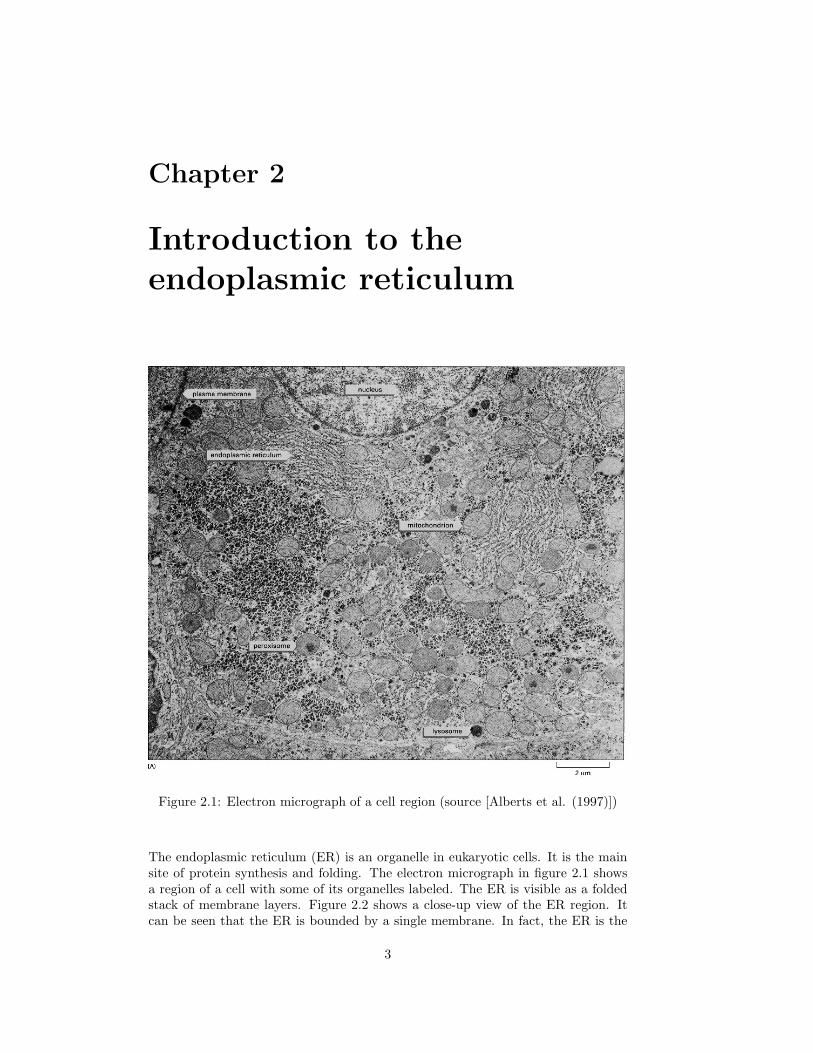
Figure 2.1: Electron micrograph of a cell region (source [Alberts et al. (1997)])
The endoplasmic reticulum (ER) is an organelle in eukaryotic cells. It is the mainsite of protein synthesis and folding. The electron micrograph in figure 2.1 showsa region of a cell with some of its organelles labeled. The ER is visible as a foldedstack of membrane layers. Figure 2.2 shows a close-up view of the ER region. Itcan be seen that the ER is bounded by a single membrane. In fact, the ER is the
3
4 CHAPTER 2. INTRODUCTION TO THE ENDOPLASMIC RETICULUM
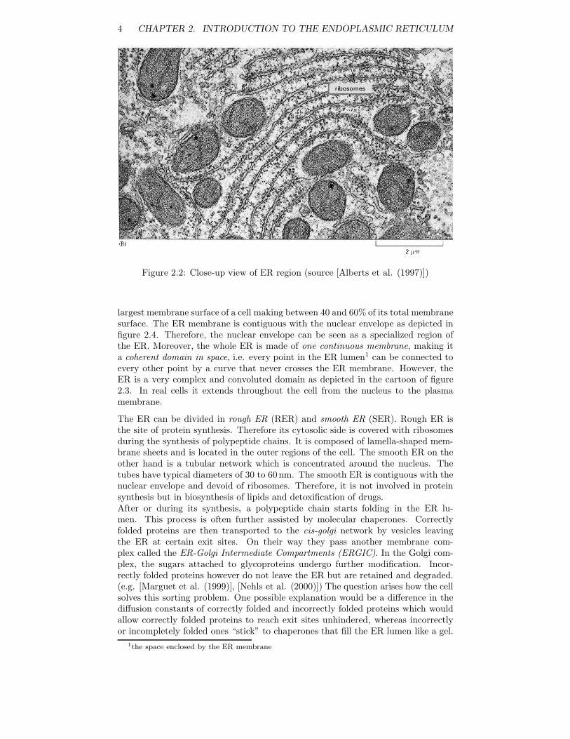
Figure 2.2: Close-up view of ER region (source [Alberts et al. (1997)])
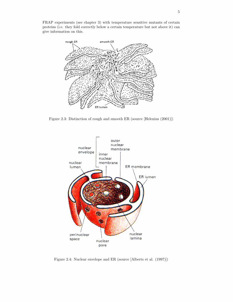
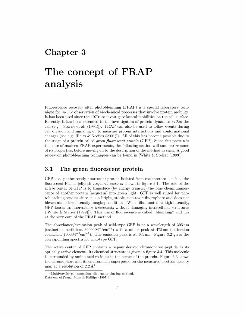
largest membrane surface of a cell making between 40 and 60% of its total membranesurface. The ER membrane is contiguous with the nuclear envelope as depicted infigure 2.4. Therefore, the nuclear envelope can be seen as a specialized region ofthe ER. Moreover, the whole ER is made of one continuous membrane, making ita coherent domain in space, i.e. every point in the ER lumen1 can be connected toevery other point by a curve that never crosses the ER membrane. However, theER is a very complex and convoluted domain as depicted in the cartoon of figure2.3. In real cells it extends throughout the cell from the nucleus to the plasmamembrane.
The ER can be divided in rough ER (RER) and smooth ER (SER). Rough ER isthe site of protein synthesis. Therefore its cytosolic side is covered with ribosomesduring the synthesis of polypeptide chains. It is composed of lamella-shaped mem-brane sheets and is located in the outer regions of the cell. The smooth ER on theother hand is a tubular network which is concentrated around the nucleus. Thetubes have typical diameters of 30 to 60 nm. The smooth ER is contiguous with thenuclear envelope and devoid of ribosomes. Therefore, it is not involved in proteinsynthesis but in biosynthesis of lipids and detoxification of drugs.After or during its synthesis, a polypeptide chain starts folding in the ER lu-men. This process is often further assisted by molecular chaperones. Correctlyfolded proteins are then transported to the cis-golgi network by vesicles leavingthe ER at certain exit sites. On their way they pass another membrane com-plex called the ER-Golgi Intermediate Compartments (ERGIC). In the Golgi com-plex, the sugars attached to glycoproteins undergo further modification. Incor-rectly folded proteins however do not leave the ER but are retained and degraded.(e.g. [Marguet et al. (1999)], [Nehls et al. (2000)]) The question arises how the cellsolves this sorting problem. One possible explanation would be a difference in thediffusion constants of correctly folded and incorrectly folded proteins which wouldallow correctly folded proteins to reach exit sites unhindered, whereas incorrectlyor incompletely folded ones “stick” to chaperones that fill the ER lumen like a gel.
1the space enclosed by the ER membrane
5
FRAP experiments (see chapter 3) with temperature sensitive mutants of certainproteins (i.e. they fold correctly below a certain temperature but not above it) cangive information on this.
Figure 2.3: Distinction of rough and smooth ER (source [Helenius (2001)])
Figure 2.4: Nuclear envelope and ER (source [Alberts et al. (1997)])

6 CHAPTER 2. INTRODUCTION TO THE ENDOPLASMIC RETICULUM
Chapter 3
The concept of FRAPanalysis
Fluorescence recovery after photobleaching (FRAP) is a special laboratory tech-nique for in-vivo observation of biochemical processes that involve protein mobility.It has been used since the 1970s to investigate lateral mobilities on the cell surface.Recently, it has been extended to the investigation of protein dynamics within thecell (e.g. [Storrie et al. (1994)]). FRAP can also be used to follow events duringcell division and signaling or to measure protein interactions and conformationalchanges (see e.g. [Reits & Neefjes (2001)]). All of this has become possible due tothe usage of a protein called green fluorescent protein (GFP). Since this protein isthe core of modern FRAP experiments, the following section will summarize someof its properties, before moving on to the description of the method as such. A goodreview on photobleaching techniques can be found in [White & Stelzer (1999)].
3.1 The green fluorescent protein
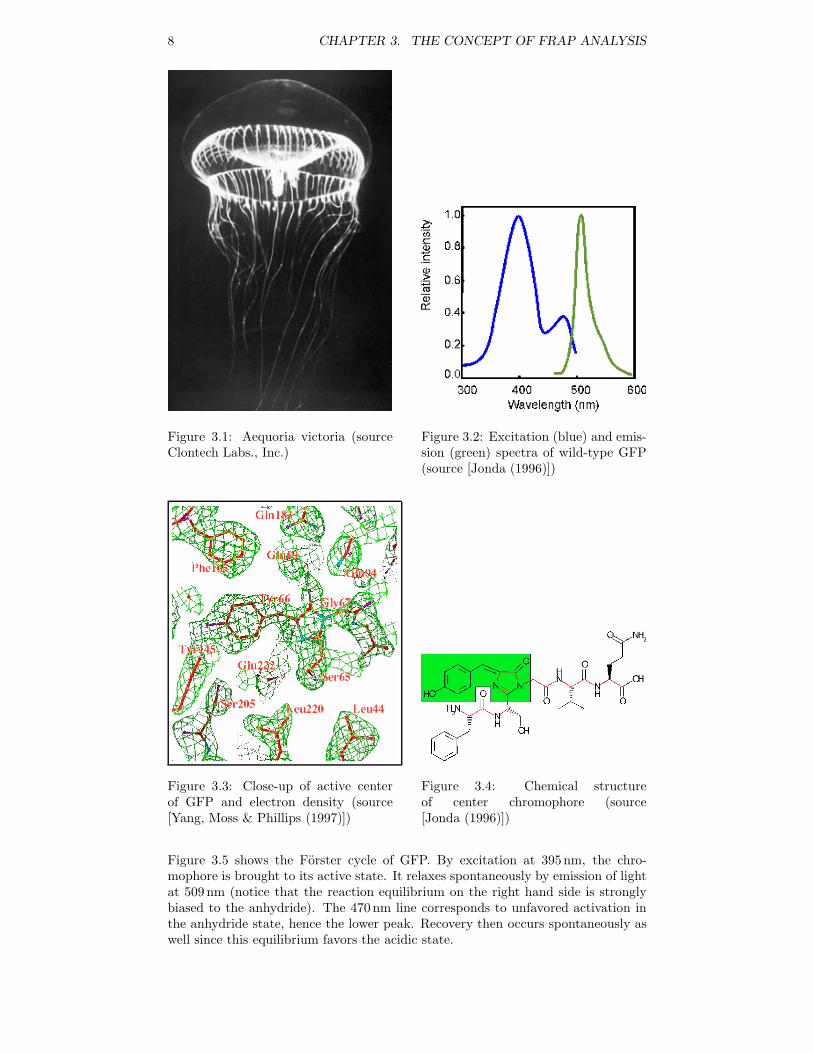
GFP is a spontaneously fluorescent protein isolated from coelenterates, such as thefluorescent Pacific jellyfish Aequoria victoria shown in figure 3.1. The role of theactive center of GFP is to transduce (by energy transfer) the blue chemilumines-cence of another protein (aequorin) into green light. GFP is well suited for pho-tobleaching studies since it is a bright, stable, non-toxic fluorophore and does notbleach under low intensity imaging conditions. When illuminated at high intensity,GFP looses its fluorescence irreversibly without damaging intracellular structures([White & Stelzer (1999)]). This loss of fluorescence is called ”bleaching” and liesat the very core of the FRAP method.
The absorbance/excitation peak of wild-type GFP is at a wavelength of 395 nm(extinction coefficient 30000 M−1cm−1) with a minor peak at 475nm (extinctioncoefficient 7000 M−1cm−1). The emission peak is at 509nm. Figure 3.2 gives thecorresponding spectra for wild-type GFP.
The active center of GFP contains a papain derived chromophore peptide as itsoptically active element. Its chemical structure is given in figure 3.4. This moleculeis surrounded by amino acid residues in the center of the protein. Figure 3.3 showsthe chromophore and its environment superposed on the measured electron densitymap at a resolution of 2.2 A1.
1Multiwavelength anomalous dispersion phasing method.Data out of [Yang, Moss & Phillips (1997)]
7
8 CHAPTER 3. THE CONCEPT OF FRAP ANALYSIS
Figure 3.1: Aequoria victoria (sourceClontech Labs., Inc.)
Figure 3.2: Excitation (blue) and emis-sion (green) spectra of wild-type GFP(source [Jonda (1996)])
Figure 3.3: Close-up of active centerof GFP and electron density (source[Yang, Moss & Phillips (1997)])
Figure 3.4: Chemical structureof center chromophore (source[Jonda (1996)])
Figure 3.5 shows the Forster cycle of GFP. By excitation at 395nm, the chro-mophore is brought to its active state. It relaxes spontaneously by emission of lightat 509 nm (notice that the reaction equilibrium on the right hand side is stronglybiased to the anhydride). The 470 nm line corresponds to unfavored activation inthe anhydride state, hence the lower peak. Recovery then occurs spontaneously aswell since this equilibrium favors the acidic state.
3.1. THE GREEN FLUORESCENT PROTEIN 9
Figure 3.5: Forster cycle of GFP fluo-rophore (source [Jonda (1996)])
Figure 3.6: Protein structure of GFP(source Clontech Labs., Inc.)
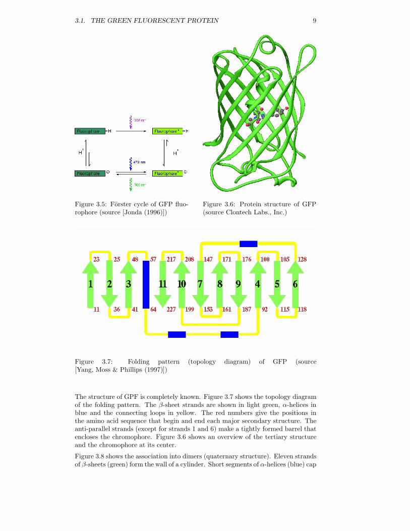
Figure 3.7: Folding pattern (topology diagram) of GFP (source[Yang, Moss & Phillips (1997)])
The structure of GPF is completely known. Figure 3.7 shows the topology diagramof the folding pattern. The β-sheet strands are shown in light green, α-helices inblue and the connecting loops in yellow. The red numbers give the positions inthe amino acid sequence that begin and end each major secondary structure. Theanti-parallel strands (except for strands 1 and 6) make a tightly formed barrel thatencloses the chromophore. Figure 3.6 shows an overview of the tertiary structureand the chromophore at its center.
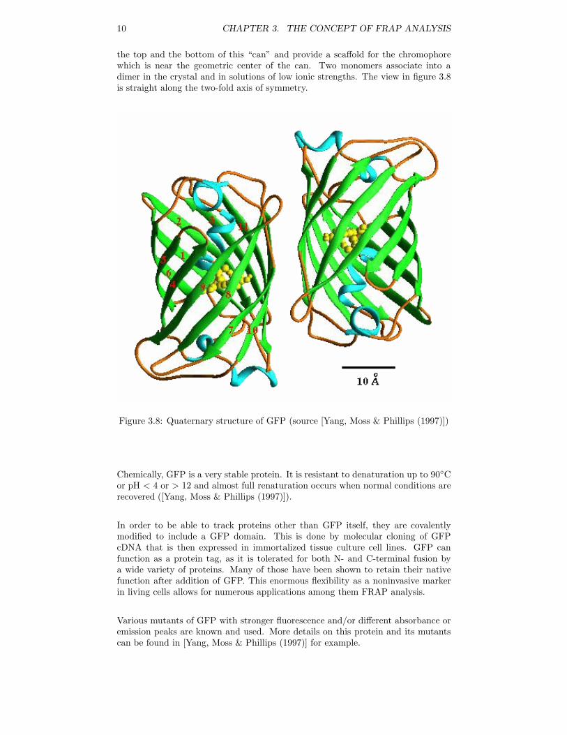
Figure 3.8 shows the association into dimers (quaternary structure). Eleven strandsof β-sheets (green) form the wall of a cylinder. Short segments of α-helices (blue) cap
10 CHAPTER 3. THE CONCEPT OF FRAP ANALYSIS
the top and the bottom of this “can” and provide a scaffold for the chromophorewhich is near the geometric center of the can. Two monomers associate into adimer in the crystal and in solutions of low ionic strengths. The view in figure 3.8is straight along the two-fold axis of symmetry.
Figure 3.8: Quaternary structure of GFP (source [Yang, Moss & Phillips (1997)])
Chemically, GFP is a very stable protein. It is resistant to denaturation up to 90Cor pH < 4 or > 12 and almost full renaturation occurs when normal conditions arerecovered ([Yang, Moss & Phillips (1997)]).
In order to be able to track proteins other than GFP itself, they are covalentlymodified to include a GFP domain. This is done by molecular cloning of GFPcDNA that is then expressed in immortalized tissue culture cell lines. GFP canfunction as a protein tag, as it is tolerated for both N- and C-terminal fusion bya wide variety of proteins. Many of those have been shown to retain their nativefunction after addition of GFP. This enormous flexibility as a noninvasive markerin living cells allows for numerous applications among them FRAP analysis.
Various mutants of GFP with stronger fluorescence and/or different absorbance oremission peaks are known and used. More details on this protein and its mutantscan be found in [Yang, Moss & Phillips (1997)] for example.
3.2. FRAP ANALYSIS 11
3.2 FRAP analysis
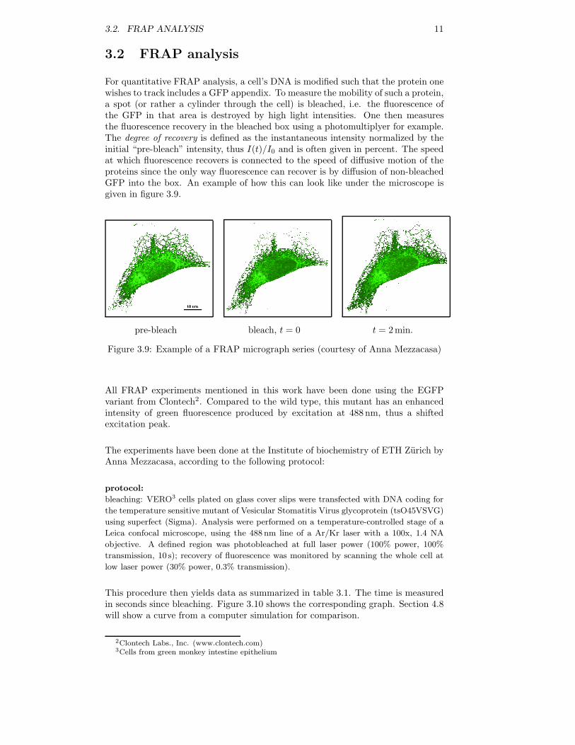
For quantitative FRAP analysis, a cell’s DNA is modified such that the protein onewishes to track includes a GFP appendix. To measure the mobility of such a protein,a spot (or rather a cylinder through the cell) is bleached, i.e. the fluorescence ofthe GFP in that area is destroyed by high light intensities. One then measuresthe fluorescence recovery in the bleached box using a photomultiplyer for example.The degree of recovery is defined as the instantaneous intensity normalized by theinitial “pre-bleach” intensity, thus I(t)/I0 and is often given in percent. The speedat which fluorescence recovers is connected to the speed of diffusive motion of theproteins since the only way fluorescence can recover is by diffusion of non-bleachedGFP into the box. An example of how this can look like under the microscope isgiven in figure 3.9.
pre-bleach bleach, t = 0 t = 2min.
Figure 3.9: Example of a FRAP micrograph series (courtesy of Anna Mezzacasa)
All FRAP experiments mentioned in this work have been done using the EGFPvariant from Clontech2. Compared to the wild type, this mutant has an enhancedintensity of green fluorescence produced by excitation at 488 nm, thus a shiftedexcitation peak.
The experiments have been done at the Institute of biochemistry of ETH Zurich byAnna Mezzacasa, according to the following protocol:
protocol:
bleaching: VERO3 cells plated on glass cover slips were transfected with DNA coding for
the temperature sensitive mutant of Vesicular Stomatitis Virus glycoprotein (tsO45VSVG)
using superfect (Sigma). Analysis were performed on a temperature-controlled stage of a
Leica confocal microscope, using the 488 nm line of a Ar/Kr laser with a 100x, 1.4 NA
objective. A defined region was photobleached at full laser power (100% power, 100%
transmission, 10 s); recovery of fluorescence was monitored by scanning the whole cell at
low laser power (30% power, 0.3% transmission).
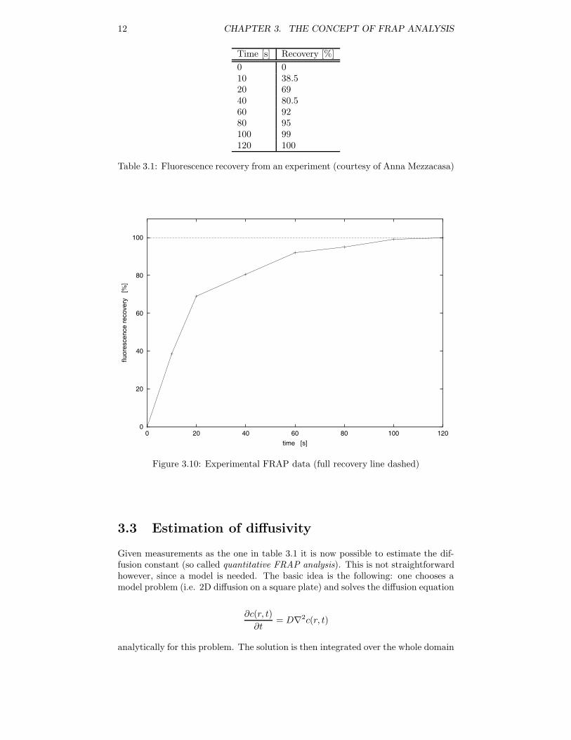
This procedure then yields data as summarized in table 3.1. The time is measuredin seconds since bleaching. Figure 3.10 shows the corresponding graph. Section 4.8will show a curve from a computer simulation for comparison.
2Clontech Labs., Inc. (www.clontech.com)3Cells from green monkey intestine epithelium
12 CHAPTER 3. THE CONCEPT OF FRAP ANALYSIS
Time [s] Recovery [%]0 010 38.520 6940 80.560 9280 95100 99120 100
Table 3.1: Fluorescence recovery from an experiment (courtesy of Anna Mezzacasa)
0
20
40
60
80
100
0 20 40 60 80 100 120
fluor
esce
nce
reco
very
[%
]
time [s]
Figure 3.10: Experimental FRAP data (full recovery line dashed)
3.3 Estimation of diffusivity
Given measurements as the one in table 3.1 it is now possible to estimate the dif-fusion constant (so called quantitative FRAP analysis). This is not straightforwardhowever, since a model is needed. The basic idea is the following: one chooses amodel problem (i.e. 2D diffusion on a square plate) and solves the diffusion equation
∂c(r, t)∂t
= D∇2c(r, t)
analytically for this problem. The solution is then integrated over the whole domain
3.3. ESTIMATION OF DIFFUSIVITY 13
to get its intensity. This intensity will be dependent on the diffusion constant Dand might for example look like this:
I =∫
Ω
c(r, t) dr = I0(1− e−kDt
)
where I0 is the pre-bleach intensity and k is a constant that depends on the geometryof Ω. This expression is then fitted to the measurement data using a nonlinear (dueto the e-function) least squares approach. Doing this will yield a value for D.
In principle, this is an easy method. The problem however is to find an appropriatemodel for protein diffusion in the ER. As will be shown in chapter 5, this modelhas some influence on the resulting D value. Since todays models lack universality,one should be careful to compare diffusion coefficients and mobile fractions betweendifferent cell lines or compartments ([Reits & Neefjes (2001)]).
3.3.1 Currently used models
The model that is commonly used in quantitative FRAP analysis is described in[Dayel, Hom & Verkman (1999)]. Hereby, the ER is modeled as a planar sheet,inclined at an angle θ to the horizontal. The vertically oriented bleach/probe beamis modeled as a uniform circular cylinder of diameter d. It is assumed that the sheetis very thin (i.e. 2D) and that the bleach time is infinitely short. The intersectionof the beam with the sheet is given by an ellipse of minor axis d/2 and majoraxis d/(2 cos θ). Then, the 2D diffusion equation for bleached GFP moving out ofthe ellipse is solved by integrating its Green’s function (i.e. superposition of pointsources). It is assumed that the diffusion of fluorescent GFP into to ellipse willexhibit the same dynamics.
Green’s function for the 2-dimensional diffusion equation on an ellipse is given by:
G(r, t) =M
4πDter2/4Dt
where M is the amount of bleached protein. This is then rewritten in dimensionlessform:
G(r, τ) =M ′
4πτer2d2/4τ
with a dimensionless time τ = Dt/d2 and a dimensionless concentration M ′ =M/d2. The concentration at point rq is then given by the convolution:
c(rq , τ) =∫
Ω
G(rq − r, τ) dr
where Ω denotes the bleached ellipse. The total observed fluorescence from theplanar ellipse at angle θ therefore is:
I(θ, τ) = A ·∫
Ω
c(rq, τ) drq
where the constant A relates the concentration of GFP to the fluorescence intensity.For planes of random orientation between angles θmin and θmax, the mean totalfluorescence is given by:
〈I(θ, τ)〉θmax
θmin=
θmax∑θmin
I(θ, τ) cos θ
θmax∑θmin
cos θ
14 CHAPTER 3. THE CONCEPT OF FRAP ANALYSIS
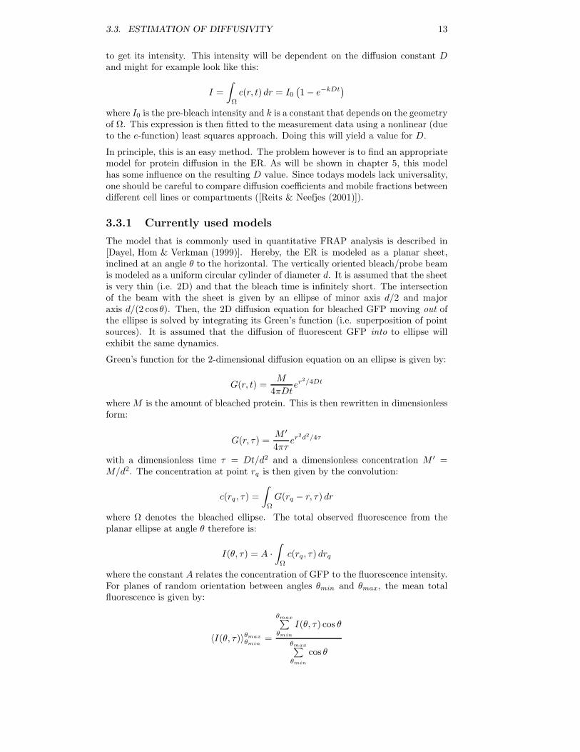
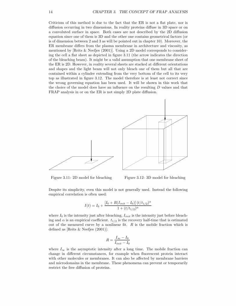
Criticism of this method is due to the fact that the ER is not a flat plate, nor isdiffusion occurring in two dimensions. In reality proteins diffuse in 3D space or ona convoluted surface in space. Both cases are not described by the 2D diffusionequation since one of them is 3D and the other one contains geometrical factors (oris of dimension between 2 and 3 as will be pointed out in chapter 10). Moreover, theER membrane differs from the plasma membrane in architecture and viscosity, asmentioned by [Reits & Neefjes (2001)]. Using a 2D model corresponds to consider-ing the cell a flat sheet as depicted in figure 3.11 (the arrow indicates the directionof the bleaching beam). It might be a valid assumption that one membrane sheet ofthe ER is 2D. However, in reality several sheets are stacked at different orientationsand shapes and the light beam will not only bleach one of them but all that arecontained within a cylinder extending from the very bottom of the cell to its verytop as illustrated in figure 3.12. The model therefore is at least not correct sincethe wrong governing equation has been used. It will be shown in this work thatthe choice of the model does have an influence on the resulting D values and thatFRAP analysis in or on the ER is not simply 2D plate diffusion.
Figure 3.11: 2D model for bleaching Figure 3.12: 3D model for bleaching
Despite its simplicity, even this model is not generally used. Instead the followingempirical correlation is often used:
I(t) = I0 +[I0 +R(Iinit − I0)] (t/t1/2)α
1 + (t/t1/2)α
where I0 is the intensity just after bleaching, Iinit is the intensity just before bleach-ing and α is an empirical coefficient. t1/2 is the recovery half-time that is estimatedout of the measured curve by a nonlinear fit. R is the mobile fraction which isdefined as [Reits & Neefjes (2001)]:
R =I∞ − I0Iinit − I0
where I∞ is the asymptotic intensity after a long time. The mobile fraction canchange in different circumstances, for example when fluorescent protein interactwith other molecules or membranes. It can also be affected by membrane barriersand microdomains in the membrane. These phenomena can prevent or temporarilyrestrict the free diffusion of proteins.
3.4. RESTATEMENT OF GOALS 15
This method yields results that generally do not differ by more than 5% from theones of the 2D model described above.
The main point of criticism of this method is its complete lack of physical relations.It might however yield better results than the 2D plate model since it is empiricallyfound by experiments.
3.4 Restatement of goals
As a conclusion it can be stated that the models used for diffusion on the ER arenot very elaborate. They could in principle be replaced by a computational modelon a “reference geometry”. The far goal of this project and its continuations isto develop a better model based on computational methods and to find a modelgeometry that accounts for the complexity and shape of a real ER. Reference runscould then be performed that relate FRAP curves (or their half-times) to D values.Or, the computational model could be controlled by an optimization strategy4 todrive its output towards the measured FRAP curve. The corresponding D valuewould then be readily available from the latest input file.
4such as Evolution Strategies or Genetic Algorithms

16 CHAPTER 3. THE CONCEPT OF FRAP ANALYSIS
Chapter 4
The simulation technique
When simulating diffusion, one has the choice among several methods such as dis-cretizing the diffusion equation and then solving the resulting system of algebraicequations, writing a symbolic solution (using Green’s function) which is then dis-cretized and solved on particles or doing a bottom-up random walk approach. Inthis work, the third will be done for various reasons, among them:
• It allows for easy generalization to arbitrary geometries as encountered inbiology.
• Realistic boundary conditions (periodic or closed-box) can easily be managed.
• Anisotropic diffusion and spatially dependent diffusion constants are easier toimplement.
• Single particles can be identified with physical entities (proteins) which allowsfor easy reproduction of FRAP data and meaningful visualizations.
• Physically, diffusion is nothing but Brownian motion (i.e. random walk) on amolecular level and the diffusion equation is just a (macroscopic) model for itusing the concept of concentrations. It is however difficult to measure or evendefine concentration on a molecular level which renders this model a littletroublesome.
4.1 On the relation of random walk and diffusion
The last point needs a little closer look. Diffusion is a physical phenomenon whichturns “order” into “disorder” and it is temperature dependent. Jan Ingenhouszhas discovered Brownian motion (i.e. thermal movement of atoms/molecules) tobe the underlying principle of such processes. By “Brownian motion” we mean itsWiener approximation by a non-differentiable continuous function for the rest ofthis work (c.f. also section 10.1.1). It can be completely characterized if the meandistance of a “jump” and the mean time between two jumps are known statistically.This forms the foundation of statistical mechanics and gas dynamics. Consider aone-dimensional Brownian motion and let a be the mean distance of a jump and nthe total number of jumps that are made to get from point 0 to point x. May sout of these n jumps be heading in the “right” direction (i.e. towards x) and n− sjumps pointing away from x (recall that this describes a 1D process). Then thetotal distance traveled is:
x = a(s− (n− s)) = a(2s− n)
17
18 CHAPTER 4. THE SIMULATION TECHNIQUE
and therefore:
s =n
2+
x
2a(4.1)
Now, let τ denote the mean time between two jumps (or the time needed to travela distance of a) and t = nτ the time to reach position x. The probability that sout of n steps are heading in the right direction is given by:
P (s, n) =(n
s
)(12
)n
(4.2)
since the elementary probability for a single step is 1/2. Herein, the followingdefinition of the binomial coefficient has been used:
(n
s
)=n(n− 1) . . . (n− s+ 1)
s!=
n!(n− s)!s!
where s! denotes the factorial of the number s. Replacing n and s by the measurablequantities t and x yields:
P (x, t) = P (s, n) =( 1
τt
2τ + x2a
)(12
) tτ
Assuming large values for n, Stirling’s formula1 can be used to approximate equation4.2 by:
P (x, t) = P (s, n) = A · B · C ·D (4.3)
where:
A =e−n
e−se−(n−s)= 1
B = exp [n lnn− s ln s− (n− s) ln(n− s)]
C = n1/2 (2πs(n− s))−1/2
D = exp [−n ln 2]
B can be further simplified by replacing s by equation 4.1, introducing the dimen-sionless length
δ =x
2ausing the identity
ln(n
2± δ)
= lnn− ln 2 + ln(
1± 2δn
)
and expanding ln(1 + α) into its Taylor series:
ln(1 + α) = α− α2
2+ . . .
Doing this and neglecting terms in δ of third and higher order results in a simplifiedexpression for the product D · B:
D · B = exp[−2δ2
n
]= exp
[− x
2τ
2a2t
]
1This formula states that for large n: n! ≈ e−nnn√
2πn
4.1. ON THE RELATION OF RANDOM WALK AND DIFFUSION 19
Introducing the diffusivity constant D for one-dimensional diffusion2:
D =a2
2τtranslates this to:
D · B = e−x24Dt
Next, the factor C is considered. Inserting equation 4.1 and using the definition oft leads to:
C = (2π)−12
(n(
n2 −
x2a
) (n2 + x
2a
)) 1
2
and after some manipulations:
C = (2π)−12 2[(t2 − x2τ
τ
a2
)( 1tτ
)]− 12
If τ and a go to zero (which is the case for real Brownian motion), τ/a2 remainsfinite, namely 1/(2D). However, τD becomes small and the term containing x2 canbe neglected compared to the first term. Taking the limit one finds:
C = (2π)−12 2τ
12 t−
12
Assembling all the results, equation 4.3 becomes:
P (x, t) = (2π)−12 2τ
12 t−
12 e−
x24Dt (4.4)
This still contains τ which has been assumed to go to zero. However, it can beinterpreted as a probability density function which is never finite for a single pointx. The probability of finding the particle in an interval (s1, s2) is thus finite:
P (s1 < s < s2) =s2∑s1
P (s, n)
Returning to the coordinates x and t, this sum can be replaced by an integral sincex varies continuously and P (s, n) is smooth.
s2∑s1
P (s, n) =∫ x2
x1
P (x, t)12a
dx
where 4.1 has been used to get an expression for dx. Defining f(x, t) = 12a P (x, t)
and using result 4.4 yields:
s2∑s1
P (s, n) =∫ x2
x1
f(x, t) dx =∫ x2
x1
(4tDπ)−12 exp
[− x2
4Dt
]dx
The function f(x, t) satisfies all requirements for a probability density function(PDF). It can be interpreted as the probability of finding a particle that started attime 0 at position 0 at position x at time t. Explicitly:
f(x, t) =1√
4πDte−
x24Dt
2according to Einstein’s result that the square deviation from the starting point is proportionalto time for a particle doing Brownian motion
20 CHAPTER 4. THE SIMULATION TECHNIQUE
The generalization to three dimensions is easy when using the fact that the probabil-ity of finding a particle at location (x, y, z) is given by the product of the elementaryprobabilities. Thus, the probability of finding a particle at position r = (x, y, z) attime t when it started off at time 0 at position ρ = (ξ, η, ζ) is given by the PDF:
f(r, ρ, t) =1
(4πDt)3/2e−
(x−ξ)2+(y−η)2+(z−ζ)2
4Dt (4.5)
One can now claim that this is nothing but the Green’s function of the followingPDE:
∂c(r, t)∂t
= D∇2c(r, t) (4.6)
Proof. Consider a finite one-dimensional domain (−L,L). The general Eigenfunc-tions on this domain are given by the periodic solutions of Helmholtz’s equation:
ϕ′′(x) + λϕ(x) = 0 x ∈ (−L,L)ϕ(x± L) = ϕ(x)
for the Eigenvalues λ. Solving this equation by separation of variables, one finds:
ϕ0 = 12L ϕk = 1√
L
sin(
2kπL x
)if k = 0
cos(
2kπL x
)if k = 0
λk =(
2kπL
)2∀k ∈ N
+0 . Green’s function for any differential equation is generally defined as:
G(x, ξ) =∞∑
k=0
1λkϕk(x)ϕk(ξ)
Accounting for time dependence in general boundary/initial value problems leads toa special Green’s function commonly called Heat Kernel since it was first discoveredfor the heat conduction equation:
K(x, ξ, t) =∞∑
k=0
ϕk(x)ϕk(ξ)e−κλkt
where κ is the “thermal conductivity”. Inserting above Eigenfunctions and -valuesand taking the limit L→∞ (infinite domain) yields:
K(x, ξ, t) =1√
4πκte−
(x−ξ)2
4κt
This function meets all requirements for a Green’s function, namely:
• Symmetry: K(x, ξ, t) = K(ξ, x, t)
• Boundary conditions: K → 0 if |x| → ∞, |ξ| → ∞ or t→∞
• PDE:∂K
∂t= κ
∂2K
∂x2
• Point source condition: limt→0
K(x, ξ, t) = δ(x− ξ) where δ(x) is the Dirac deltadistribution
4.2. SIMULATION ALGORITHM OUTLINE 21
Using the cartesian product theorem which states that the heat kernel for a productdomain is given by the product of the heat kernels of the elementary domains, theheat kernel for the infinite three-dimensional space can be derived as:
KΩ = KΩ1 ·KΩ2 ·KΩ3 =1
(4πκt)3/2e−
(x−ξ)2+(y−η)2+(z−ζ)2
4κt (4.7)
and therefore, the solution of equation 4.6 is given by:
c(r, t) =∫ ∞
−∞K(r, ρ, t)c0(ρ) dρ
where c0 is the initial distribution of c and r = (x, y, z) and ρ = (ξ, η, ζ) are vectorsin space. Replacing κ with D in equation 4.7 recovers equation 4.5, which completesthis proof.
If f(x, t) in equation 4.5 is the heat kernel (or Green’s function) of the diffusion equa-tion 4.6, all superpositions of f(x, t) are solutions of the diffusion equation. Sincef(x, t) has been derived starting from the initial distribution c0(x, t) = δ(x− ξ) andall equations are linear, it is the elementary solution of diffusion. Therefore, diffu-sion is equal to random walk (Brownian motion) under the following assumptions(made to derive 4.5):
1. Large number of Brownian jumps (i.e. n→∞)
2. Mean time between jumps infinitely small (i.e. τ → 0)
3. Mean distance per jump infinitely small (i.e. a→ 0)
4. Quadratic approximation for PDF in equation 4.3
Diffusion can thus be seen as a macroscopic second order statistical model for Brow-nian motion or, inverting the argument, Brownian motion is the underlying micro-scopic reason of diffusion and its Wiener approximation is accurate except for errorsintroduced by not exactly fulfilling assumptions 1 to 3 in a simulation code.
4.2 Simulation algorithm outline
Since this project is about the simulation of diffusive processes on a molecular level,the usage of non-interacting particles performing a random walk seems to be theright approach. Particle interactions (i.e. potentials) can be neglected since at thissize and speed, inertia plays virtually no role and charges are very small (if presentat all) compared to the molecular weight of a protein.
One could object that random walk simulations only converge towards the solutionof the diffusion equation as 1/
√N whereas other algorithms like Particle Strength
Exchange converge as 1/N2 (see [Cottet & Koumoutsakos (2000)]). However, con-vergence is not needed since we are not solving the diffusion equation but perform-ing direct random walk without assuming above points and without defining a localparticle concentration. To quote [Perrin (1906)]: “One might encounter instanceswhere using a function without a derivative would be simpler than using one thatcan be differentiated. When this happens, the mathematical study of irregular con-tinua will prove its practical value.”3. Therefore, the simulation algorithm proceedsas follows:
3Jean Perrin, 1906. Later Nobel Prize for his work on Brownian motion
22 CHAPTER 4. THE SIMULATION TECHNIQUE
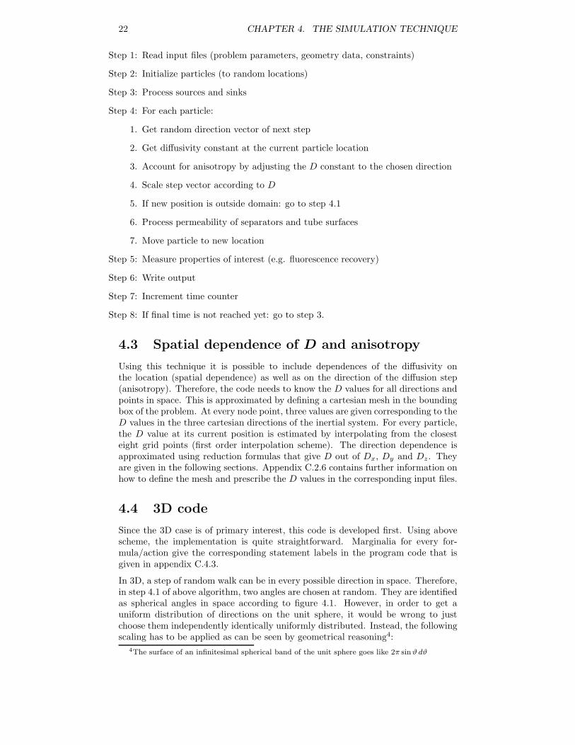
Step 1: Read input files (problem parameters, geometry data, constraints)
Step 2: Initialize particles (to random locations)
Step 3: Process sources and sinks
Step 4: For each particle:
1. Get random direction vector of next step
2. Get diffusivity constant at the current particle location
3. Account for anisotropy by adjusting the D constant to the chosen direction
4. Scale step vector according to D
5. If new position is outside domain: go to step 4.1
6. Process permeability of separators and tube surfaces
7. Move particle to new location
Step 5: Measure properties of interest (e.g. fluorescence recovery)
Step 6: Write output
Step 7: Increment time counter
Step 8: If final time is not reached yet: go to step 3.
4.3 Spatial dependence of D and anisotropy
Using this technique it is possible to include dependences of the diffusivity onthe location (spatial dependence) as well as on the direction of the diffusion step(anisotropy). Therefore, the code needs to know the D values for all directions andpoints in space. This is approximated by defining a cartesian mesh in the boundingbox of the problem. At every node point, three values are given corresponding to theD values in the three cartesian directions of the inertial system. For every particle,the D value at its current position is estimated by interpolating from the closesteight grid points (first order interpolation scheme). The direction dependence isapproximated using reduction formulas that give D out of Dx, Dy and Dz. Theyare given in the following sections. Appendix C.2.6 contains further information onhow to define the mesh and prescribe the D values in the corresponding input files.
4.4 3D code
Since the 3D case is of primary interest, this code is developed first. Using abovescheme, the implementation is quite straightforward. Marginalia for every for-mula/action give the corresponding statement labels in the program code that isgiven in appendix C.4.3.
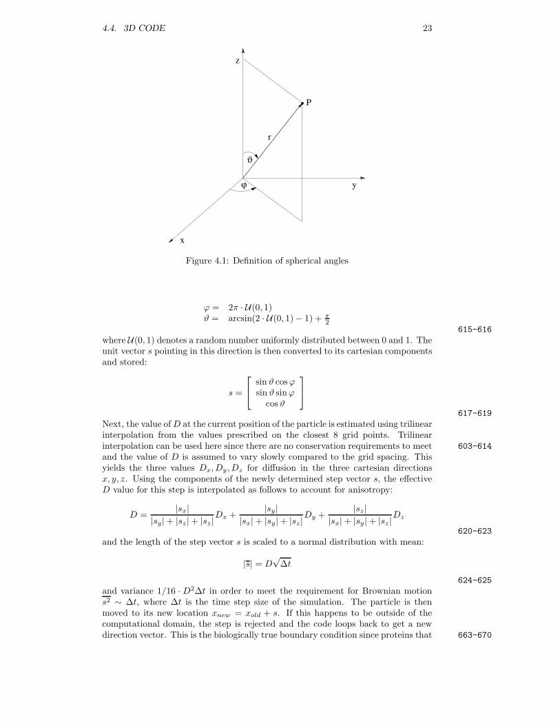
In 3D, a step of random walk can be in every possible direction in space. Therefore,in step 4.1 of above algorithm, two angles are chosen at random. They are identifiedas spherical angles in space according to figure 4.1. However, in order to get auniform distribution of directions on the unit sphere, it would be wrong to justchoose them independently identically uniformly distributed. Instead, the followingscaling has to be applied as can be seen by geometrical reasoning4:
4The surface of an infinitesimal spherical band of the unit sphere goes like 2π sinϑ dϑ
4.4. 3D CODE 23
x
y
z
r
ϑ
ϕ
P
Figure 4.1: Definition of spherical angles
ϕ = 2π · U(0, 1)ϑ = arcsin(2 · U(0, 1)− 1) + π
2615-616
where U(0, 1) denotes a random number uniformly distributed between 0 and 1. Theunit vector s pointing in this direction is then converted to its cartesian componentsand stored:
s =
sinϑ cosϕ
sinϑ sinϕcosϑ
617-619Next, the value ofD at the current position of the particle is estimated using trilinearinterpolation from the values prescribed on the closest 8 grid points. Trilinearinterpolation can be used here since there are no conservation requirements to meet 603-614and the value of D is assumed to vary slowly compared to the grid spacing. Thisyields the three values Dx, Dy, Dz for diffusion in the three cartesian directionsx, y, z. Using the components of the newly determined step vector s, the effectiveD value for this step is interpolated as follows to account for anisotropy:
D =|sx|
|sy|+ |sz|+ |sz |Dx +
|sy||sx|+ |sy|+ |sz|
Dy +|sz|
|sx|+ |sy|+ |sz |Dz
620-623and the length of the step vector s is scaled to a normal distribution with mean:
|s| = D√
∆t
624-625and variance 1/16 · D2∆t in order to meet the requirement for Brownian motions2 ∼ ∆t, where ∆t is the time step size of the simulation. The particle is thenmoved to its new location xnew = xold + s. If this happens to be outside of thecomputational domain, the step is rejected and the code loops back to get a newdirection vector. This is the biologically true boundary condition since proteins that 663-670
24 CHAPTER 4. THE SIMULATION TECHNIQUE
move in the ER lumen cannot leave the ER by diffusing through its membrane. Theystay inside the lumen until they get exported by vesicular transport or degraded(both can be modeled as sinks: see section 4.6).
4.5 2D code
The 2D version of the code only differs from the 3D version in the following points:the third component of any vector is zero for all times and for a random step onlyϕ is chosen and interpreted as polar angle in the plane z = 0:
ϕ = 2π · U(0, 1)
129The step vector is:
s =[
cosϕsinϕ
]
130-131and the effective D value is then given by:
D =|sx|
|sx|+ |sy|Dx +
|sy||sx|+ |sy|
Dy
132-134The rest (i.e. scaling and movement) remains unchanged. Marginalia refer tostatement labels in its implementation as printed in appendix C.4.2.
4.6 Adding sources and sinks
In order to be able to model protein exportation and production, point sourcesand Gaussian sinks are introduced. A source is defined by its location (x, y, z)in space and its strength S. The location can be an arbitrary point inside thecomputational domain (points outside the domain are ignored) and the strength isan integer number giving the number of particles that are produced/swallowed perunit time (not per time step !). Whereas a source simply puts the desired numberof particles to its location (i.e. all particles are placed in the same spot), a sinkneeds to have some sort of “attractive behavior” since it will hardly ever happenthat a particle visits exactly the location of the sink. This is done using a Gaussianattractor characteristic, meaning that a particle gets swallowed at a probability of:
P =1
σ√
2πexp
[− d
2σ2
](4.8)
556-567where d is the distance from the particle to the sink and the standard deviation is:
σ =(
3S∆tVBBox
4πN
) 13
(4.9)
where S is the strength of the sink, ∆t the simulation step size, N the total num-ber of particles and VBBox the volume of the bounding box of the computationaldomain. In order to ensure that particles close to the sink get removed first, theyare processed in ascending order of their distance to the sink. Therefore, all parti-cles are first ranked according to their distance. This is efficiently done using the“indexx” function given in appendix C.4.8. The algorithm for every sink is now:
4.7. SEPARATOR PLANES BUILD COMPARTMENTS 25
Step 1: Calculate distance to sink for all particles
Step 2: Rank particles by ascending distance
Step 3: Calculate standard deviation of sink using 4.9
Step 4: For each particle
1. Calculate probability of particle to get removed using 4.8
2. if U(0, 1) < P remove particle and increment counter
3. if enough particles have been removed: STOP
For the definition of sources and sinks in the corresponding input file see appendixC.2.2.
4.7 Separator planes build compartments
Cells need different compartments that are separated from each other by a mem-brane and contain different concentrations and/or species. A very crude modelfor this in introduced by the concept of separator planes. These planes extendthroughout the computational domain and are characterized by their location andpermeability. If at any time a particle attempts to cross such a plane, the move isonly allowed at a certain probability. Thus the step vector of Brownian motion isupdated as: 642-662
s =s if U(0, 1) < ν0 else
where U(0, 1) is a random number, uniformly distributed between 0 and 1 and0 ν 1 is the permeability of the separator. Details on how separators aredefined and used are contained in appendix C.2.4.
4.8 Simulating FRAP analysis
Using above simulation technique, it is straightforward to implement FRAP ana-lysis (c.f. section 3.2). The only thing that needs to be changed is the initialparticle distribution in step 2 of the algorithm. It is modified such that only parti-cles at (random) locations outside of some bleached area are accepted. An exam-ple of a resulting initial distribution is shown in figure 4.2 where the view line iscollinear with the bleaching light beam (i.e. from above) and the square cylinder(x, y, z)|2 x 3, 2 y 3 has been “bleached”. In step 5 of the algorithm onpage 22, the number of particles that are inside the bleached box is counted inevery time step. Plotting this number (normalized by the total number of particles)yields fluorescence recovery curves similar to those found in experiments (e.g. fig-ure 3.10). Figure 4.3 shows such a curve from a computer experiment in 3D using10000 particles. The dashed line indicates the pre-bleach value, i.e. the value whena completely homogeneous particle distribution has been recovered (100% recovery).
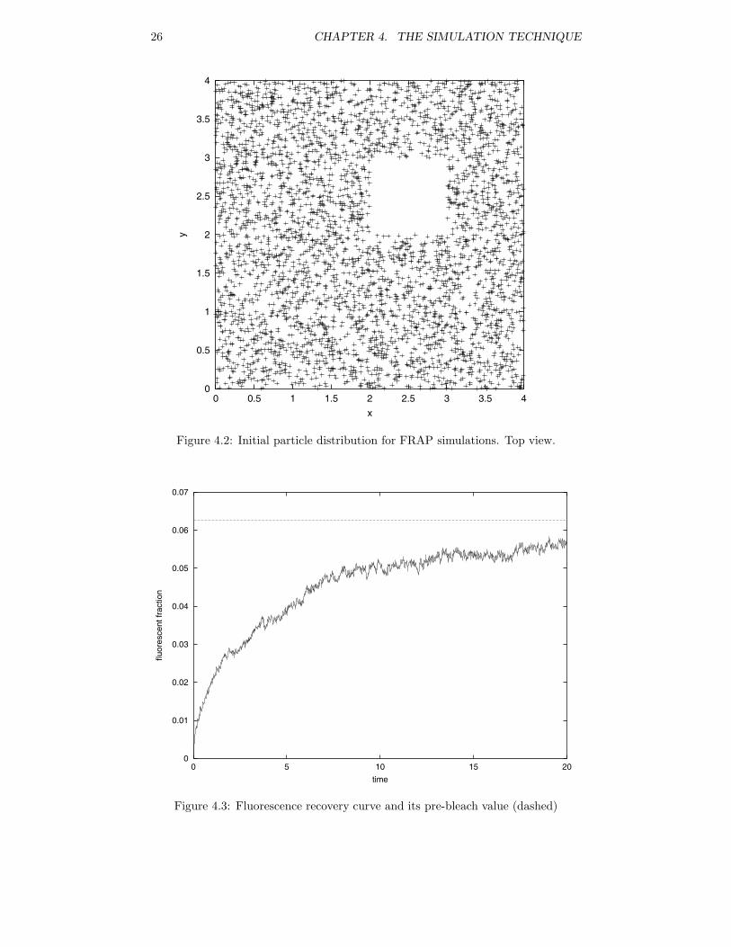
26 CHAPTER 4. THE SIMULATION TECHNIQUE
0
0.5
1
1.5
2
2.5
3
3.5
4
0 0.5 1 1.5 2 2.5 3 3.5 4
y
x
Figure 4.2: Initial particle distribution for FRAP simulations. Top view.
0
0.01
0.02
0.03
0.04
0.05
0.06
0.07
0 5 10 15 20
fluor
esce
nt fr
actio
n
time
Figure 4.3: Fluorescence recovery curve and its pre-bleach value (dashed)
Chapter 5
FRAP analysis of 2D and 3Dspace diffusion
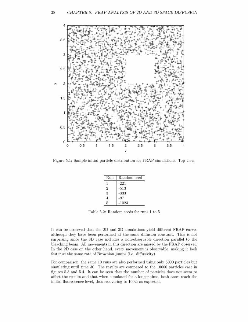
Using the methods described in chapter 4, 2D and 3D simulations are performed.The computational domain for the 3D case is the cube [0; 4]× [0; 4]× [0; 4] and forthe 2D case it is the corresponding square [0; 4]× [0; 4]. The boundary conditionsare “closed-box”, i.e. no particle is allowed to enter or exit the domain. This is thebiologically correct boundary condition since lumen proteins are never allowed toexit the endoplasmic reticulum and the ER is not a periodic domain. An exampleof the initial condition is depicted in a top view in figure 5.1. The square (cylinder)[2; 3] × [2; 3] is bleached, meaning that is contains no fluorescent particles at timezero.
All runs have the following parameters in common:
Parameter ValueNumber of space particles 10000Number of surface particles 0Time step size 0.005Final time of simulation 20Separators noneSources none
Table 5.1: Common parameters for 2D and 3D runs
For every case, 5 runs are performed starting from different initial random seedvalues1. The random seeds of table 5.2 (need to be negative and integer) are usedfor the random number generator given in appendix C.4.9.
All 5 runs are averaged at every time step to get the final fluorescence value at thattime. This ensemble averaging reduces the risk of spurious effects introduced by therandom number generator or an accidentally chosen “special” configuration. Figure5.2 shows the result.
1This not only implies different particle distributions but also different behavior wherever ran-dom numbers are involved, e.g. for permeabilities, etc.
27
28 CHAPTER 5. FRAP ANALYSIS OF 2D AND 3D SPACE DIFFUSION
0
0.5
1
1.5
2
2.5
3
3.5
4
0 0.5 1 1.5 2 2.5 3 3.5 4
y
x
Figure 5.1: Sample initial particle distribution for FRAP simulations. Top view.
Run Random seed1 -2212 -5133 -3334 -975 -1023
Table 5.2: Random seeds for runs 1 to 5
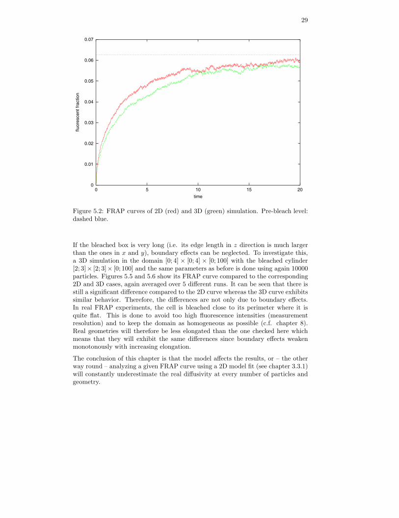
It can be observed that the 2D and 3D simulations yield different FRAP curvesalthough they have been performed at the same diffusion constant. This is notsurprising since the 3D case includes a non-observable direction parallel to thebleaching beam. All movements in this direction are missed by the FRAP observer.In the 2D case on the other hand, every movement is observable, making it lookfaster at the same rate of Brownian jumps (i.e. diffusivity).
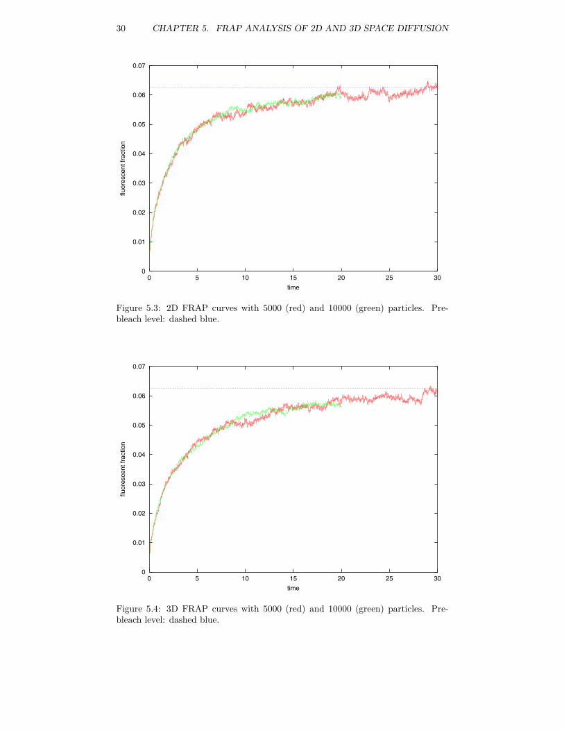
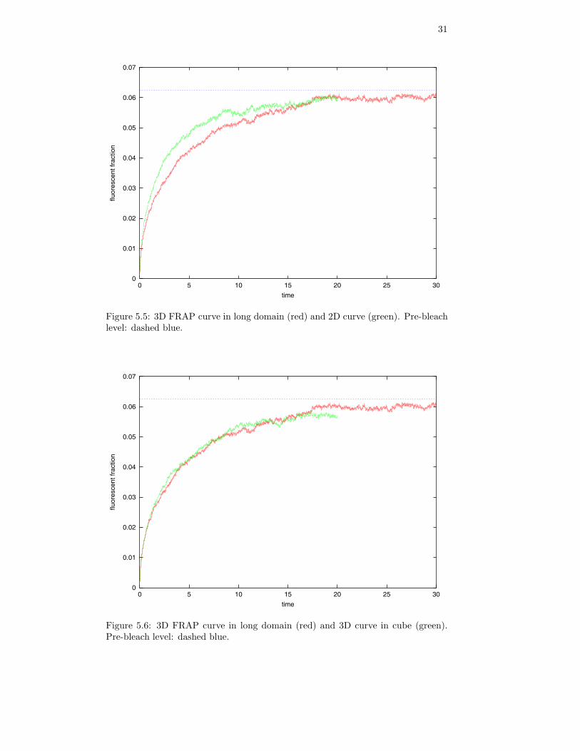
For comparison, the same 10 runs are also performed using only 5000 particles butsimulating until time 30. The results are compared to the 10000 particles case infigures 5.3 and 5.4. It can be seen that the number of particles does not seem toaffect the results and that when simulated for a longer time, both cases reach theinitial fluorescence level, thus recovering to 100% as expected.
29
0
0.01
0.02
0.03
0.04
0.05
0.06
0.07
0 5 10 15 20
fluor
esce
nt fr
actio
n
time
Figure 5.2: FRAP curves of 2D (red) and 3D (green) simulation. Pre-bleach level:dashed blue.
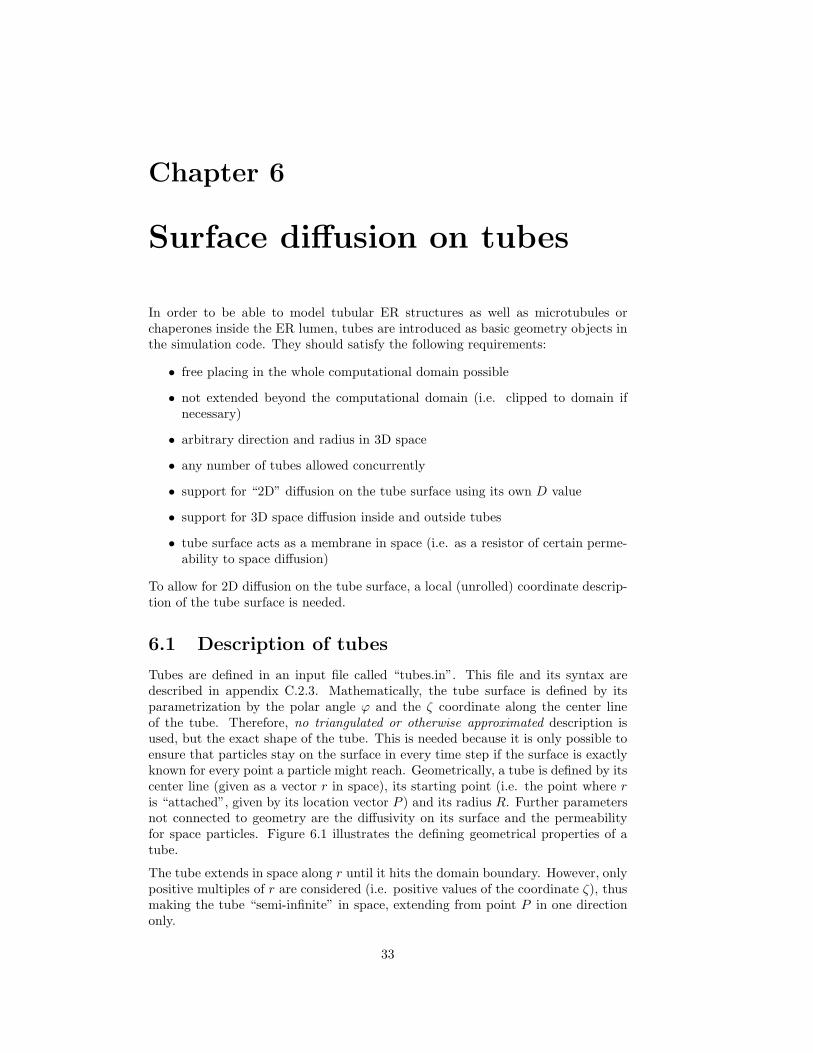
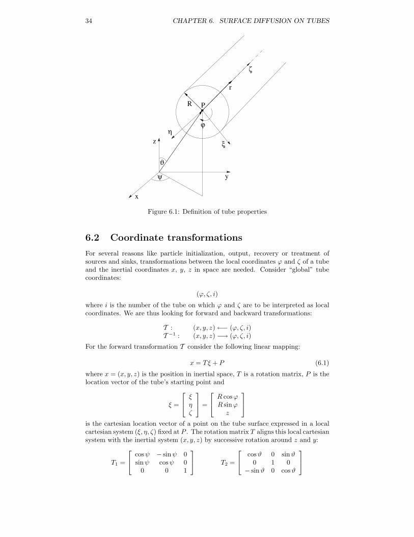
If the bleached box is very long (i.e. its edge length in z direction is much largerthan the ones in x and y), boundary effects can be neglected. To investigate this,a 3D simulation in the domain [0; 4] × [0; 4] × [0; 100] with the bleached cylinder[2; 3]× [2; 3]× [0; 100] and the same parameters as before is done using again 10000particles. Figures 5.5 and 5.6 show its FRAP curve compared to the corresponding2D and 3D cases, again averaged over 5 different runs. It can be seen that there isstill a significant difference compared to the 2D curve whereas the 3D curve exhibitssimilar behavior. Therefore, the differences are not only due to boundary effects.In real FRAP experiments, the cell is bleached close to its perimeter where it isquite flat. This is done to avoid too high fluorescence intensities (measurementresolution) and to keep the domain as homogeneous as possible (c.f. chapter 8).Real geometries will therefore be less elongated than the one checked here whichmeans that they will exhibit the same differences since boundary effects weakenmonotonously with increasing elongation.
The conclusion of this chapter is that the model affects the results, or – the otherway round – analyzing a given FRAP curve using a 2D model fit (see chapter 3.3.1)will constantly underestimate the real diffusivity at every number of particles andgeometry.
30 CHAPTER 5. FRAP ANALYSIS OF 2D AND 3D SPACE DIFFUSION
0
0.01
0.02
0.03
0.04
0.05
0.06
0.07
0 5 10 15 20 25 30
fluor
esce
nt fr
actio
n
time
Figure 5.3: 2D FRAP curves with 5000 (red) and 10000 (green) particles. Pre-bleach level: dashed blue.
0
0.01
0.02
0.03
0.04
0.05
0.06
0.07
0 5 10 15 20 25 30
fluor
esce
nt fr
actio
n
time
Figure 5.4: 3D FRAP curves with 5000 (red) and 10000 (green) particles. Pre-bleach level: dashed blue.
31
0
0.01
0.02
0.03
0.04
0.05
0.06
0.07
0 5 10 15 20 25 30
fluor
esce
nt fr
actio
n
time
Figure 5.5: 3D FRAP curve in long domain (red) and 2D curve (green). Pre-bleachlevel: dashed blue.
0
0.01
0.02
0.03
0.04
0.05
0.06
0.07
0 5 10 15 20 25 30
fluor
esce
nt fr
actio
n
time
Figure 5.6: 3D FRAP curve in long domain (red) and 3D curve in cube (green).Pre-bleach level: dashed blue.

32 CHAPTER 5. FRAP ANALYSIS OF 2D AND 3D SPACE DIFFUSION
Chapter 6
Surface diffusion on tubes
In order to be able to model tubular ER structures as well as microtubules orchaperones inside the ER lumen, tubes are introduced as basic geometry objects inthe simulation code. They should satisfy the following requirements:
• free placing in the whole computational domain possible
• not extended beyond the computational domain (i.e. clipped to domain ifnecessary)
• arbitrary direction and radius in 3D space
• any number of tubes allowed concurrently
• support for “2D” diffusion on the tube surface using its own D value
• support for 3D space diffusion inside and outside tubes
• tube surface acts as a membrane in space (i.e. as a resistor of certain perme-ability to space diffusion)
To allow for 2D diffusion on the tube surface, a local (unrolled) coordinate descrip-tion of the tube surface is needed.
6.1 Description of tubes
Tubes are defined in an input file called “tubes.in”. This file and its syntax aredescribed in appendix C.2.3. Mathematically, the tube surface is defined by itsparametrization by the polar angle ϕ and the ζ coordinate along the center lineof the tube. Therefore, no triangulated or otherwise approximated description isused, but the exact shape of the tube. This is needed because it is only possible toensure that particles stay on the surface in every time step if the surface is exactlyknown for every point a particle might reach. Geometrically, a tube is defined by itscenter line (given as a vector r in space), its starting point (i.e. the point where ris “attached”, given by its location vector P ) and its radius R. Further parametersnot connected to geometry are the diffusivity on its surface and the permeabilityfor space particles. Figure 6.1 illustrates the defining geometrical properties of atube.
The tube extends in space along r until it hits the domain boundary. However, onlypositive multiples of r are considered (i.e. positive values of the coordinate ζ), thusmaking the tube “semi-infinite” in space, extending from point P in one directiononly.
33
34 CHAPTER 6. SURFACE DIFFUSION ON TUBES
r
R
ζ
ξ
ϑ
ϕ
ψ
z
y
P
x
η
Figure 6.1: Definition of tube properties
6.2 Coordinate transformations
For several reasons like particle initialization, output, recovery or treatment ofsources and sinks, transformations between the local coordinates ϕ and ζ of a tubeand the inertial coordinates x, y, z in space are needed. Consider “global” tubecoordinates:
(ϕ, ζ, i)
where i is the number of the tube on which ϕ and ζ are to be interpreted as localcoordinates. We are thus looking for forward and backward transformations:
T : (x, y, z)←− (ϕ, ζ, i)T −1 : (x, y, z) −→ (ϕ, ζ, i)
For the forward transformation T consider the following linear mapping:
x = Tξ + P (6.1)
where x = (x, y, z) is the position in inertial space, T is a rotation matrix, P is thelocation vector of the tube’s starting point and
ξ =
ξηζ
=
R cosϕR sinϕz
is the cartesian location vector of a point on the tube surface expressed in a localcartesian system (ξ, η, ζ) fixed at P . The rotation matrix T aligns this local cartesiansystem with the inertial system (x, y, z) by successive rotation around z and y:
T1 =
cosψ − sinψ 0
sinψ cosψ 00 0 1
T2 =
cosϑ 0 sinϑ
0 1 0− sinϑ 0 cosϑ
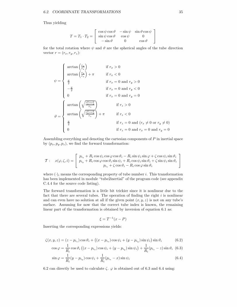
6.2. COORDINATE TRANSFORMATIONS 35
Thus yielding
T = T1 · T2 =
cosψ cosϑ − sinψ sinϑ cosψ
sinψ cosϑ cosψ 0− sinϑ 0 cosϑ
for the total rotation where ψ and ϑ are the spherical angles of the tube directionvector r = (rx, ry , rz):
ψ =
arctan(
ry
rx
)if rx > 0
arctan(
ry
rx
)+ π if rx < 0
π2 if rx = 0 and ry > 0
−π2 if rx = 0 and ry < 0
0 if rx = 0 and ry = 0
ϑ =
arctan(√
r2x+r2
y
rz
)if rz > 0
arctan(√
r2x+r2
y
rz
)+ π if rz < 0
π2 if rz = 0 and (rx = 0 or ry = 0)
0 if rz = 0 and rx = 0 and ry = 0
Assembling everything and denoting the cartesian components of P in inertial spaceby (px, py, pz), we find the forward transformation:
T : x(ϕ, ζ, i) =
pix +Ri cosψi cosϕ cosϑi −Ri sinψi sinϕ+ ζ cosψi sinϑi
piy +Ri cosϕ cosϑi sinψi +Ri cosψi sinϑi + ζ sinψi sinϑi
piz + ζ cosϑi −Ri cosϕ sinϑi
where (·)i means the corresponding property of tube number i. This transformationhas been implemented in module “tube2inertial” of the program code (see appendixC.4.4 for the source code listing).
The forward transformation is a little bit trickier since it is nonlinear due to thefact that there are several tubes. The operation of finding the right i is nonlinearand can even have no solution at all if the given point (x, y, z) is not on any tube’ssurface. Assuming for now that the correct tube index is known, the remaininglinear part of the transformation is obtained by inversion of equation 6.1 as:
ξ = T−1(x− P )
Inserting the corresponding expressions yields:
ζ(x, y, z) = (z − piz) cosϑi +((x− pix) cosψi + (y − piy ) sinψi
)sinϑi (6.2)
cosϕ =1Ri
cosϑi
((x− pix) cosψi + (y − piy) sinψi
)+
1Ri
(piz − z) sinϑi (6.3)
sinϕ =1Ri
(y − piy) cosψi +1Ri
(pix − x) sinψi (6.4)
6.2 can directly be used to calculate ζ. ϕ is obtained out of 6.3 and 6.4 using:
36 CHAPTER 6. SURFACE DIFFUSION ON TUBES
ϕ(x, y, z) =
arctan(
sin ϕcos ϕ
)if cosϕ > 0
arctan(
sin ϕcos ϕ
)+ π if cosϕ < 0
π2 if cosϕ = 0 and sinϕ > 0
−π2 if cosϕ = 0 and sinϕ < 0
0 if cosϕ = 0 and sinϕ = 0
(6.5)
The nonlinear part of finding i can be done using a simple algorithm like:
Step 1: i = 0
Step 2: for every tube j do
1. calculate orthogonal distance to tube center line
2. if distance is less than a certain tolerance: i = j
3. if i = 0 go to step 2, else STOP
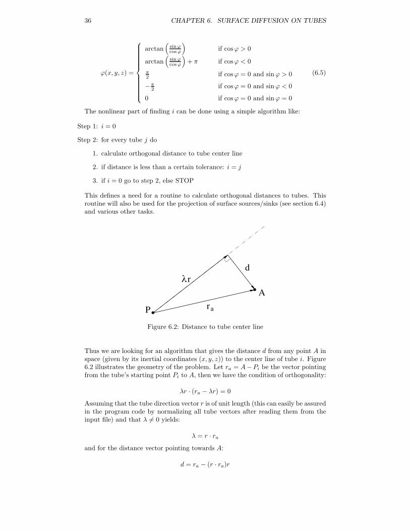
This defines a need for a routine to calculate orthogonal distances to tubes. Thisroutine will also be used for the projection of surface sources/sinks (see section 6.4)and various other tasks.
ra
λr
P
A
d
Figure 6.2: Distance to tube center line
Thus we are looking for an algorithm that gives the distance d from any point A inspace (given by its inertial coordinates (x, y, z)) to the center line of tube i. Figure6.2 illustrates the geometry of the problem. Let ra = A−Pi be the vector pointingfrom the tube’s starting point Pi to A, then we have the condition of orthogonality:
λr · (ra − λr) = 0
Assuming that the tube direction vector r is of unit length (this can easily be assuredin the program code by normalizing all tube vectors after reading them from theinput file) and that λ = 0 yields:
λ = r · raand for the distance vector pointing towards A:
d = ra − (r · ra)r
6.3. SURFACE DIFFUSION 37
Its length is:
|d| =√|ra|2 − r · ra (6.6)
This formula is implemented in the program module “dist to tube”. See appendixC.4.6 for further details on it.
Using equation 6.6, the algorithm outlined above and equations 6.2 to 6.5, it is nowpossible to complete the backward transformation T −1 which has been implementedin module “inertial2tube” (see appendix C.4.5).
6.3 Surface diffusion
Since particles that diffuse on the tube surfaces only have two degrees of freedom,a different motion than the one described in section 4.4 is performed. The particlesare moved in local cylindrical coordinates (ϕ, ζ) on the tube. First, the direction ofthe step is chosen as if the surface was unrolled in a plane:
ϑ = 2π · U(0, 1)
594with U(0, 1) being a uniformly distributed random number between 0 and 1. Thenthe length of the step is estimated as:
|s| = N (Dsurf
√∆t,
116D2
surf∆t)
595-597where N (µ, σ2) denotes a Gaussian random number with mean µ and variance σ2
and Dsurf is the surface diffusion coefficient on the tube1. The new cylindricalangle on the tube is then given by:
ϕn+1 = ϕn +1R|s| cosϑ mod 2π
and the new axial coordinate is: 598-601
ζn+1 = ζn + |s| sinϑ
This new location is now transformed to inertial coordinates (x, y, z) and the particleis moved. Using this procedure ensures that surface particles always remain exactlyon the surface. If the move would result in a position outside of the computationaldomain, it is rejected and a new step is chosen.
6.4 Sources and sinks on tubes
To complete the picture, sources and sinks are also implemented on tubes. Accord-ing to appendix C.2.2, they are defined using the same input file as space sources.However, the code needs to check whether the given location of the source is real-ly on a tube’s surface. If this is not the case (what will be most probable), it isprojected onto the closest tube surface as follows:
Let ra be the vector pointing from the starting point of the closest tube Pi to thelocation of the source xs: ra = xs−Pi. Then, the vector by which the source needs
1only isotropic diffusion with constant diffusivity is considered for tubes since otherwise it couldnot be assured that the end point of a step is on the tube again.
38 CHAPTER 6. SURFACE DIFFUSION ON TUBES
to be displaced is given by:
b = (d−Ri) [r(r · ra)− ra] (6.7)
where d is the distance from xs to the center line of the closest tube (see the end ofsection 6.2 for details on how this distance is calculated). Therefore, each surfacesource/sink is preprocessed with:367-396
Step 1: Calculate distance to every tube surface (distance to center line minus tuberadius)
Step 2: Choose closest tube i
Step 3: Move source by adding b to its position (see 6.7)
Step 4: If source is now outside domain: delete it
Once the sources and sinks are displaced to meet all constraints, they work as spacesources/sinks would do. Details have already been mentioned in section 4.6. Theonly difference is that surface sources produce “surface particles” (i.e. particles thatmove on the surface only) whereas space sources produce particles that diffuse in3D space. The same applies for sinks.
6.5 FRAP analysis at different angles
Using the preliminaries introduced above, it is now possible to perform simulationswith particles that move on the surface of a 3D shape, in this case tubes. The ques-tion to be addressed is whether this 2D diffusion (since the particles only have twodegrees of freedom) is equivalent to flat plate 2D diffusion in terms of FRAP results.It seems reasonable that the recovered D value of a FRAP experiment depends onthe tilting angle of the tube. A tube viewed from the side (i.e. perpendicular to itscenter line) is expected to be more “plate-like” than a tube viewed along its centerline.
FRAP simulations are performed using a tube at different angles. The simulationsare done using 10000 particles that diffuse on the tube surface only doing homoge-neous and isotropic diffusion with D = 0.4. The computational domain is the cube[0; 4] × [0; 4] × [0; 4] and the simulation is run for 4000 time steps up to time 20.Table 6.1 summarizes the tubes that are used one after the other.
Angle Direction vector Starting point0 (1.0, 0.0, 0.0) (0.0, 2.5, 2.0)20 (0.9397, 0.0, 0.3420) (-3.0, 2.5, 0.0)45 (1.0, 0.0, 1.0) (0.5, 2.5, 0.0)60 (0.5, 0.0, 0.866) (1.3453, 2.5, 0.0)85 (0.087156, 0.0, 0.9962) (2.325, 2.5, 0.0)
Table 6.1: Tubes for FRAP analysis
No separators, sources or sinks are present. The bleached area is [2; 3]× [2; 3]× [0; 4]and the view is parallel to the z axis of the inertial system. Therefore, the bleachedspot is larger than the tubes in diameter (i.e. it does not only contain tube surfacebut also blank space). The tubes are all parallel to the xz-plane and the tiltingangle (denoted by θ) is the angle between the tube center line and the xy-plane.
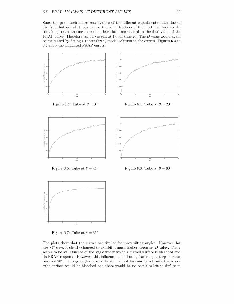
6.5. FRAP ANALYSIS AT DIFFERENT ANGLES 39
Since the pre-bleach fluorescence values of the different experiments differ due tothe fact that not all tubes expose the same fraction of their total surface to thebleaching beam, the measurements have been normalized to the final value of theFRAP curve. Therefore, all curves end at 1.0 for time 20. The D value would againbe estimated by fitting a (normalized) model solution to the curves. Figures 6.3 to6.7 show the simulated FRAP curves.
0
0.2
0.4
0.6
0.8
1
1.2
0 5 10 15 20
norm
aliz
ed fl
uore
scen
ce r
ecov
ery
time
Figure 6.3: Tube at θ = 0
0
0.2
0.4
0.6
0.8
1
1.2
0 5 10 15 20
norm
aliz
ed fl
uore
scen
ce r
ecov
ery
time
Figure 6.4: Tube at θ = 20
0
0.2
0.4
0.6
0.8
1
1.2
0 5 10 15 20
norm
aliz
ed fl
uore
scen
ce r
ecov
ery
time
Figure 6.5: Tube at θ = 45
0
0.2
0.4
0.6
0.8
1
1.2
0 5 10 15 20
norm
aliz
ed fl
uore
scen
ce r
ecov
ery
time
Figure 6.6: Tube at θ = 60
0
0.2
0.4
0.6
0.8
1
1.2
0 5 10 15 20
norm
aliz
ed fl
uore
scen
ce r
ecov
ery
time
Figure 6.7: Tube at θ = 85
The plots show that the curves are similar for most tilting angles. However, forthe 85 case, it clearly changed to exhibit a much higher apparent D value. Thereseems to be an influence of the angle under which a curved surface is bleached andits FRAP response. However, this influence is nonlinear, featuring a steep increasetowards 90. Tilting angles of exactly 90 cannot be considered since the wholetube surface would be bleached and there would be no particles left to diffuse in
40 CHAPTER 6. SURFACE DIFFUSION ON TUBES
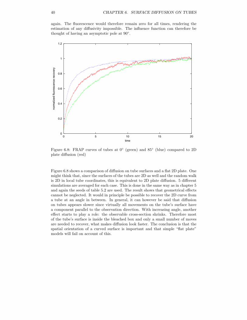
again. The fluorescence would therefore remain zero for all times, rendering theestimation of any diffusivity impossible. The influence function can therefore bethought of having an asymptotic pole at 90.
0
0.2
0.4
0.6
0.8
1
1.2
0 5 10 15 20
norm
aliz
ed fl
uore
scen
ce r
ecov
ery
time
Figure 6.8: FRAP curves of tubes at 0 (green) and 85 (blue) compared to 2Dplate diffusion (red)
Figure 6.8 shows a comparison of diffusion on tube surfaces and a flat 2D plate. Onemight think that, since the surfaces of the tubes are 2D as well and the random walkis 2D in local tube coordinates, this is equivalent to 2D plate diffusion. 5 differentsimulations are averaged for each case. This is done in the same way as in chapter 5and again the seeds of table 5.2 are used. The result shows that geometrical effectscannot be neglected. It would in principle be possible to recover the 2D curve froma tube at an angle in between. In general, it can however be said that diffusionon tubes appears slower since virtually all movements on the tube’s surface havea component parallel to the observation direction. With increasing angle, anothereffect starts to play a role: the observable cross-section shrinks. Therefore mostof the tube’s surface is inside the bleached box and only a small number of movesare needed to recover, what makes diffusion look faster. The conclusion is that thespatial orientation of a curved surface is important and that simple “flat plate”models will fail on account of this.
Chapter 7
Combining surface and spacediffusion
This chapter will briefly describe how simulations using both kinds of particles– surface and space – are implemented. Since the simulations are done withoutparticle interactions (see section 4.2 for reasoning), the only obvious change neededis a flag bit to every particle that tells whether the particle moves in space or on atube.
However, since tube surfaces are interpreted as membranes, they have interactionswith particles insofar that surface particles are bound to them and space particlesare not allowed to cross them (or are only allowed to cross them at a certain prob-ability). The former interaction has already been accounted for in section 6.3 byconstruction of the random walk. The latter interaction needs some more attention.
As can be seen from appendix C.2.3, the tube definition file not only contains itsgeometrical properties and the surface diffusion constant but also a permeability.This permeability corresponds to the probability at which a space particle is allowedto cross the tube surface given it attempts to do so. Therefore, at every time stepit is checked for every particle whether it attempts to cross a tube’s surface. If thisis the case, its step vector is updated as: 630-641
s =s if U(0, 1) < µi
0 else (7.1)
where U(0, 1) is a random number, uniformly distributed between 0 and 1 and0 µi 1 is the permeability of the surface of tube i. The complete algorithmproceeds as follows:
Step 1: r1 = distance to tube i at old position xold
Step 2: r2 = distance to tube i at new position xnew
Step 3: if (r1 − Ri)(r2 − Ri) < 0 then update step vector according to 7.1, else leaveit untouched (Ri denotes the radius of tube i).
The implementation can be found in appendix 4.4 on lines 630 to 641.
Now it is possible to have both kinds of particles in the same simulation and the roleof the tubes can be varied from impermeable to “not felt”. Figures 7.1 and 7.2 showexample visualizations of such simulations using a single tube. Only a small numberof particles is shown in order to keep the image clear. Space particles are visualizedby green spheres, surface particles by orange ones. The tube is represented by
41
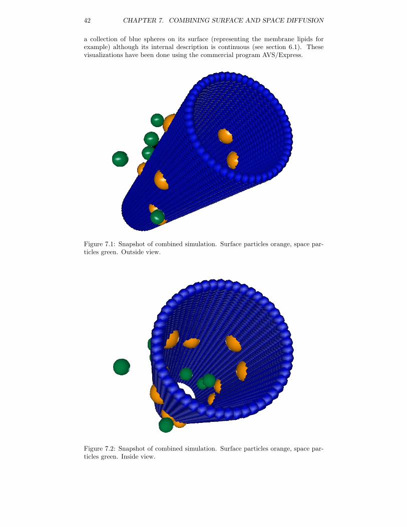
42 CHAPTER 7. COMBINING SURFACE AND SPACE DIFFUSION
a collection of blue spheres on its surface (representing the membrane lipids forexample) although its internal description is continuous (see section 6.1). Thesevisualizations have been done using the commercial program AVS/Express.
Figure 7.1: Snapshot of combined simulation. Surface particles orange, space par-ticles green. Outside view.
Figure 7.2: Snapshot of combined simulation. Surface particles orange, space par-ticles green. Inside view.
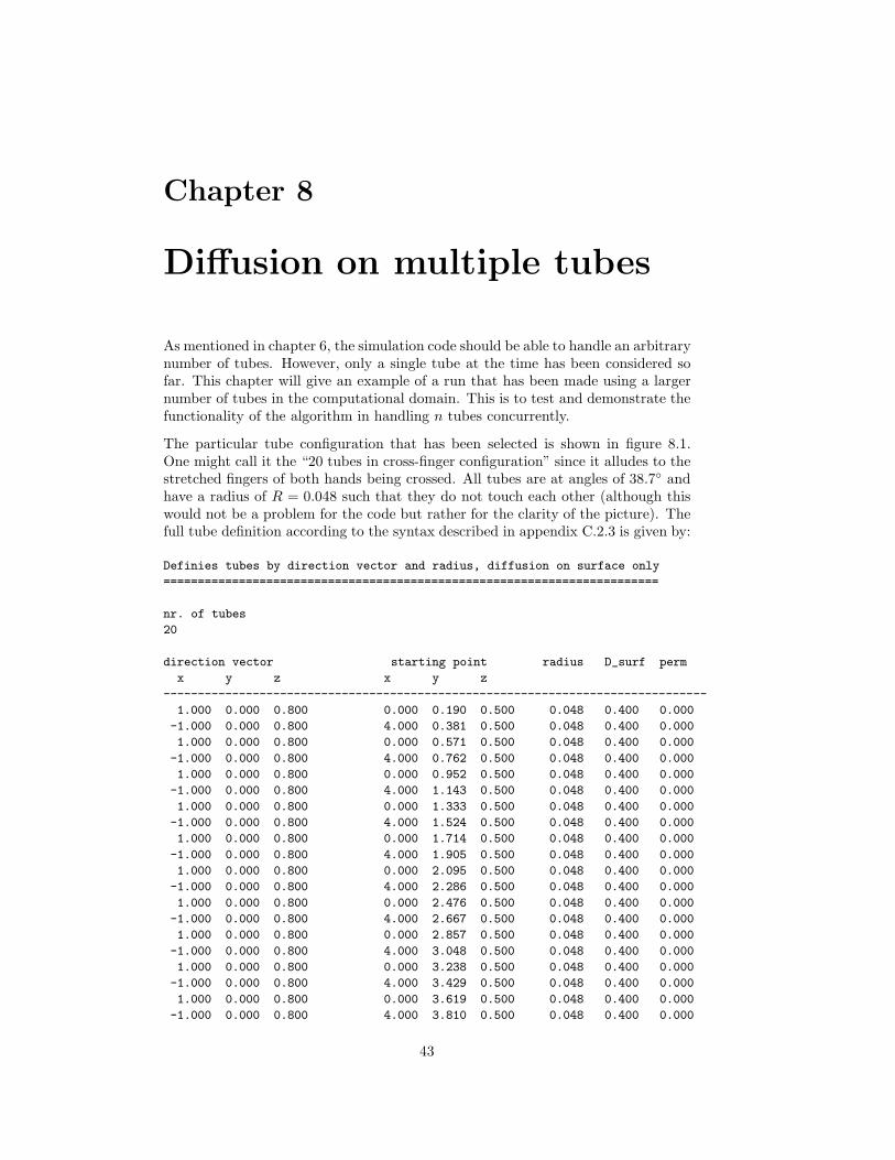
Chapter 8
Diffusion on multiple tubes
As mentioned in chapter 6, the simulation code should be able to handle an arbitrarynumber of tubes. However, only a single tube at the time has been considered sofar. This chapter will give an example of a run that has been made using a largernumber of tubes in the computational domain. This is to test and demonstrate thefunctionality of the algorithm in handling n tubes concurrently.
The particular tube configuration that has been selected is shown in figure 8.1.One might call it the “20 tubes in cross-finger configuration” since it alludes to thestretched fingers of both hands being crossed. All tubes are at angles of 38.7 andhave a radius of R = 0.048 such that they do not touch each other (although thiswould not be a problem for the code but rather for the clarity of the picture). Thefull tube definition according to the syntax described in appendix C.2.3 is given by:
Definies tubes by direction vector and radius, diffusion on surface only
========================================================================
nr. of tubes
20
direction vector starting point radius D_surf perm
x y z x y z
-------------------------------------------------------------------------------
1.000 0.000 0.800 0.000 0.190 0.500 0.048 0.400 0.000
-1.000 0.000 0.800 4.000 0.381 0.500 0.048 0.400 0.000
1.000 0.000 0.800 0.000 0.571 0.500 0.048 0.400 0.000
-1.000 0.000 0.800 4.000 0.762 0.500 0.048 0.400 0.000
1.000 0.000 0.800 0.000 0.952 0.500 0.048 0.400 0.000
-1.000 0.000 0.800 4.000 1.143 0.500 0.048 0.400 0.000
1.000 0.000 0.800 0.000 1.333 0.500 0.048 0.400 0.000
-1.000 0.000 0.800 4.000 1.524 0.500 0.048 0.400 0.000
1.000 0.000 0.800 0.000 1.714 0.500 0.048 0.400 0.000
-1.000 0.000 0.800 4.000 1.905 0.500 0.048 0.400 0.000
1.000 0.000 0.800 0.000 2.095 0.500 0.048 0.400 0.000
-1.000 0.000 0.800 4.000 2.286 0.500 0.048 0.400 0.000
1.000 0.000 0.800 0.000 2.476 0.500 0.048 0.400 0.000
-1.000 0.000 0.800 4.000 2.667 0.500 0.048 0.400 0.000
1.000 0.000 0.800 0.000 2.857 0.500 0.048 0.400 0.000
-1.000 0.000 0.800 4.000 3.048 0.500 0.048 0.400 0.000
1.000 0.000 0.800 0.000 3.238 0.500 0.048 0.400 0.000
-1.000 0.000 0.800 4.000 3.429 0.500 0.048 0.400 0.000
1.000 0.000 0.800 0.000 3.619 0.500 0.048 0.400 0.000
-1.000 0.000 0.800 4.000 3.810 0.500 0.048 0.400 0.000
43
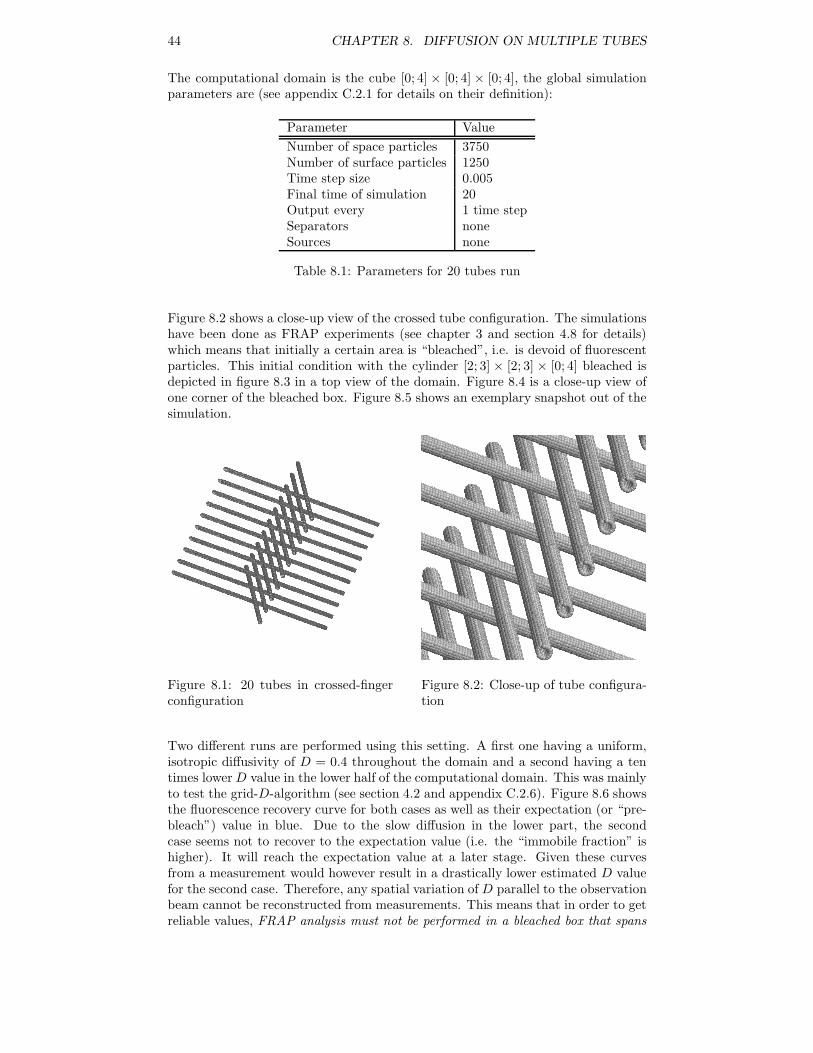
44 CHAPTER 8. DIFFUSION ON MULTIPLE TUBES
The computational domain is the cube [0; 4] × [0; 4] × [0; 4], the global simulationparameters are (see appendix C.2.1 for details on their definition):
Parameter ValueNumber of space particles 3750Number of surface particles 1250Time step size 0.005Final time of simulation 20Output every 1 time stepSeparators noneSources none
Table 8.1: Parameters for 20 tubes run
Figure 8.2 shows a close-up view of the crossed tube configuration. The simulationshave been done as FRAP experiments (see chapter 3 and section 4.8 for details)which means that initially a certain area is “bleached”, i.e. is devoid of fluorescentparticles. This initial condition with the cylinder [2; 3] × [2; 3] × [0; 4] bleached isdepicted in figure 8.3 in a top view of the domain. Figure 8.4 is a close-up view ofone corner of the bleached box. Figure 8.5 shows an exemplary snapshot out of thesimulation.
Figure 8.1: 20 tubes in crossed-fingerconfiguration
Figure 8.2: Close-up of tube configura-tion
Two different runs are performed using this setting. A first one having a uniform,isotropic diffusivity of D = 0.4 throughout the domain and a second having a tentimes lowerD value in the lower half of the computational domain. This was mainlyto test the grid-D-algorithm (see section 4.2 and appendix C.2.6). Figure 8.6 showsthe fluorescence recovery curve for both cases as well as their expectation (or “pre-bleach”) value in blue. Due to the slow diffusion in the lower part, the secondcase seems not to recover to the expectation value (i.e. the “immobile fraction” ishigher). It will reach the expectation value at a later stage. Given these curvesfrom a measurement would however result in a drastically lower estimated D valuefor the second case. Therefore, any spatial variation of D parallel to the observationbeam cannot be reconstructed from measurements. This means that in order to getreliable values, FRAP analysis must not be performed in a bleached box that spans
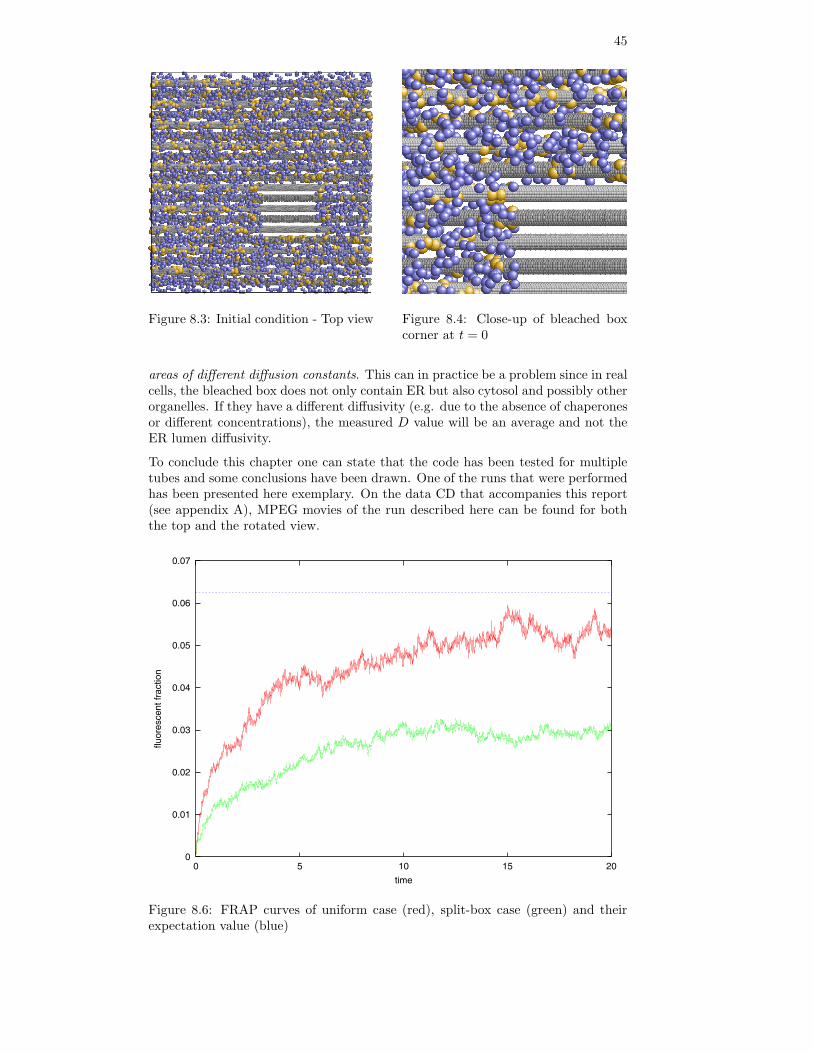
45
Figure 8.3: Initial condition - Top view Figure 8.4: Close-up of bleached boxcorner at t = 0
areas of different diffusion constants. This can in practice be a problem since in realcells, the bleached box does not only contain ER but also cytosol and possibly otherorganelles. If they have a different diffusivity (e.g. due to the absence of chaperonesor different concentrations), the measured D value will be an average and not theER lumen diffusivity.
To conclude this chapter one can state that the code has been tested for multipletubes and some conclusions have been drawn. One of the runs that were performedhas been presented here exemplary. On the data CD that accompanies this report(see appendix A), MPEG movies of the run described here can be found for boththe top and the rotated view.
0
0.01
0.02
0.03
0.04
0.05
0.06
0.07
0 5 10 15 20
fluor
esce
nt fr
actio
n
time
Figure 8.6: FRAP curves of uniform case (red), split-box case (green) and theirexpectation value (blue)
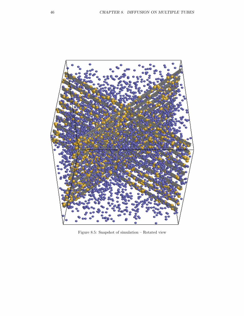
46 CHAPTER 8. DIFFUSION ON MULTIPLE TUBES
Figure 8.5: Snapshot of simulation – Rotated view
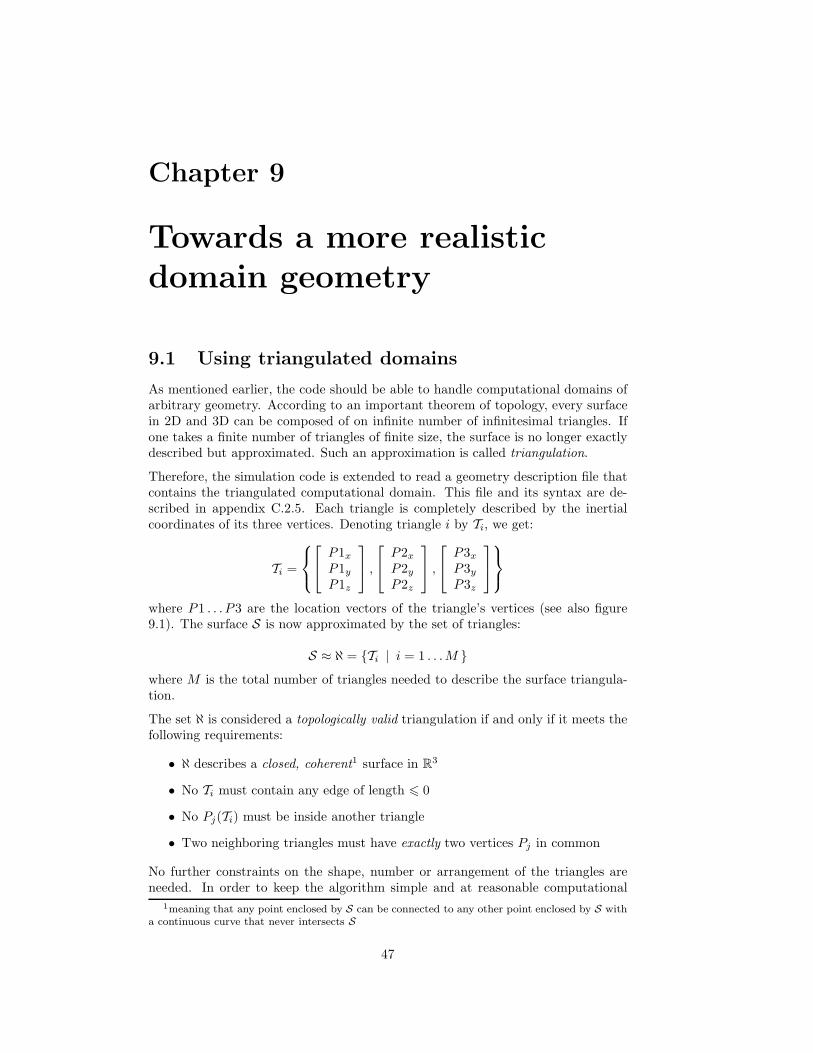
Chapter 9
Towards a more realisticdomain geometry
9.1 Using triangulated domains
As mentioned earlier, the code should be able to handle computational domains ofarbitrary geometry. According to an important theorem of topology, every surfacein 2D and 3D can be composed of on infinite number of infinitesimal triangles. Ifone takes a finite number of triangles of finite size, the surface is no longer exactlydescribed but approximated. Such an approximation is called triangulation.
Therefore, the simulation code is extended to read a geometry description file thatcontains the triangulated computational domain. This file and its syntax are de-scribed in appendix C.2.5. Each triangle is completely described by the inertialcoordinates of its three vertices. Denoting triangle i by Ti, we get:
Ti =
P1x
P1y
P1z
, P2x
P2y
P2z
, P3x
P3y
P3z
where P1 . . . P3 are the location vectors of the triangle’s vertices (see also figure9.1). The surface S is now approximated by the set of triangles:
S ≈ ℵ = Ti | i = 1 . . .M where M is the total number of triangles needed to describe the surface triangula-tion.
The set ℵ is considered a topologically valid triangulation if and only if it meets thefollowing requirements:
• ℵ describes a closed, coherent1 surface in R3
• No Ti must contain any edge of length 0
• No Pj(Ti) must be inside another triangle
• Two neighboring triangles must have exactly two vertices Pj in common
No further constraints on the shape, number or arrangement of the triangles areneeded. In order to keep the algorithm simple and at reasonable computational
1meaning that any point enclosed by S can be connected to any other point enclosed by S witha continuous curve that never intersects S
47
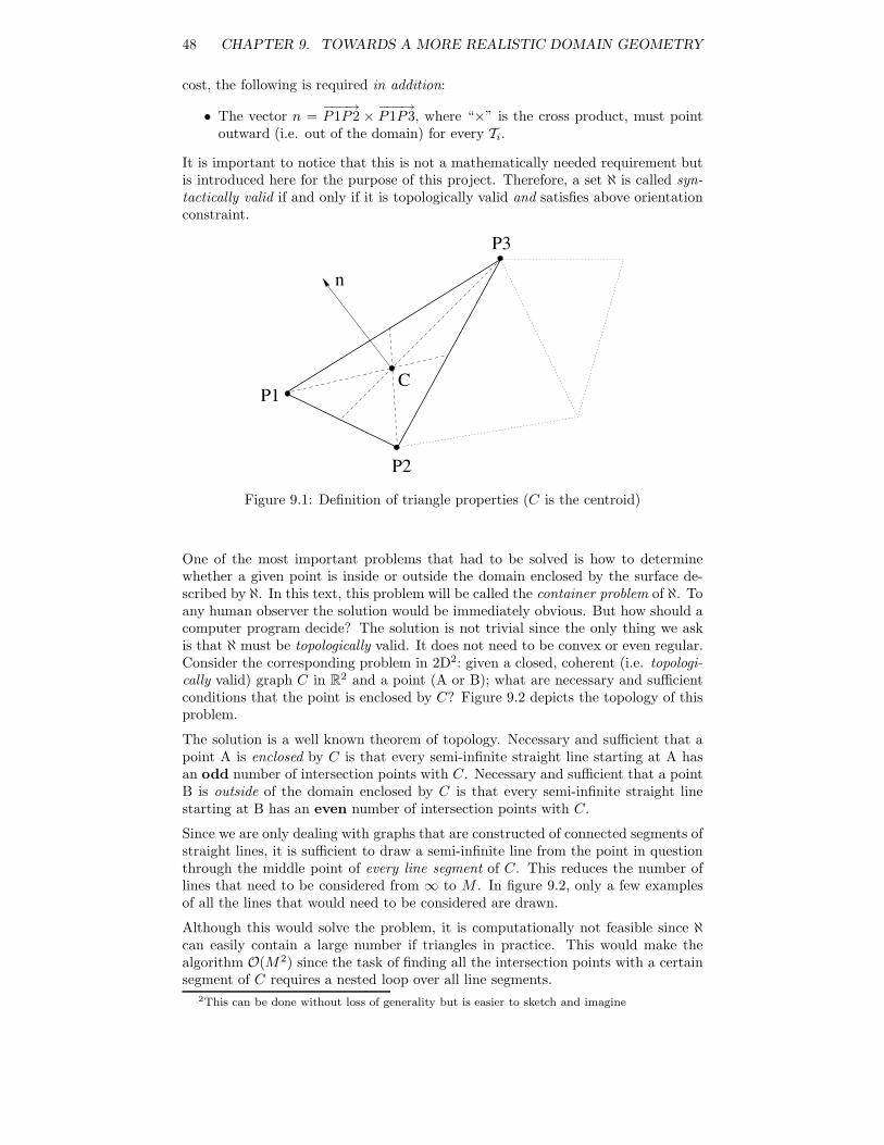
48 CHAPTER 9. TOWARDS A MORE REALISTIC DOMAIN GEOMETRY
cost, the following is required in addition:
• The vector n =−−−→P1P2 × −−−→P1P3, where “×” is the cross product, must point
outward (i.e. out of the domain) for every Ti.
It is important to notice that this is not a mathematically needed requirement butis introduced here for the purpose of this project. Therefore, a set ℵ is called syn-tactically valid if and only if it is topologically valid and satisfies above orientationconstraint.
P1
P2
P3
C
n
Figure 9.1: Definition of triangle properties (C is the centroid)
One of the most important problems that had to be solved is how to determinewhether a given point is inside or outside the domain enclosed by the surface de-scribed by ℵ. In this text, this problem will be called the container problem of ℵ. Toany human observer the solution would be immediately obvious. But how should acomputer program decide? The solution is not trivial since the only thing we askis that ℵ must be topologically valid. It does not need to be convex or even regular.Consider the corresponding problem in 2D2: given a closed, coherent (i.e. topologi-cally valid) graph C in R
2 and a point (A or B); what are necessary and sufficientconditions that the point is enclosed by C? Figure 9.2 depicts the topology of thisproblem.
The solution is a well known theorem of topology. Necessary and sufficient that apoint A is enclosed by C is that every semi-infinite straight line starting at A hasan odd number of intersection points with C. Necessary and sufficient that a pointB is outside of the domain enclosed by C is that every semi-infinite straight linestarting at B has an even number of intersection points with C.
Since we are only dealing with graphs that are constructed of connected segments ofstraight lines, it is sufficient to draw a semi-infinite line from the point in questionthrough the middle point of every line segment of C. This reduces the number oflines that need to be considered from ∞ to M . In figure 9.2, only a few examplesof all the lines that would need to be considered are drawn.
Although this would solve the problem, it is computationally not feasible since ℵcan easily contain a large number if triangles in practice. This would make thealgorithm O(M2) since the task of finding all the intersection points with a certainsegment of C requires a nested loop over all line segments.
2This can be done without loss of generality but is easier to sketch and imagine
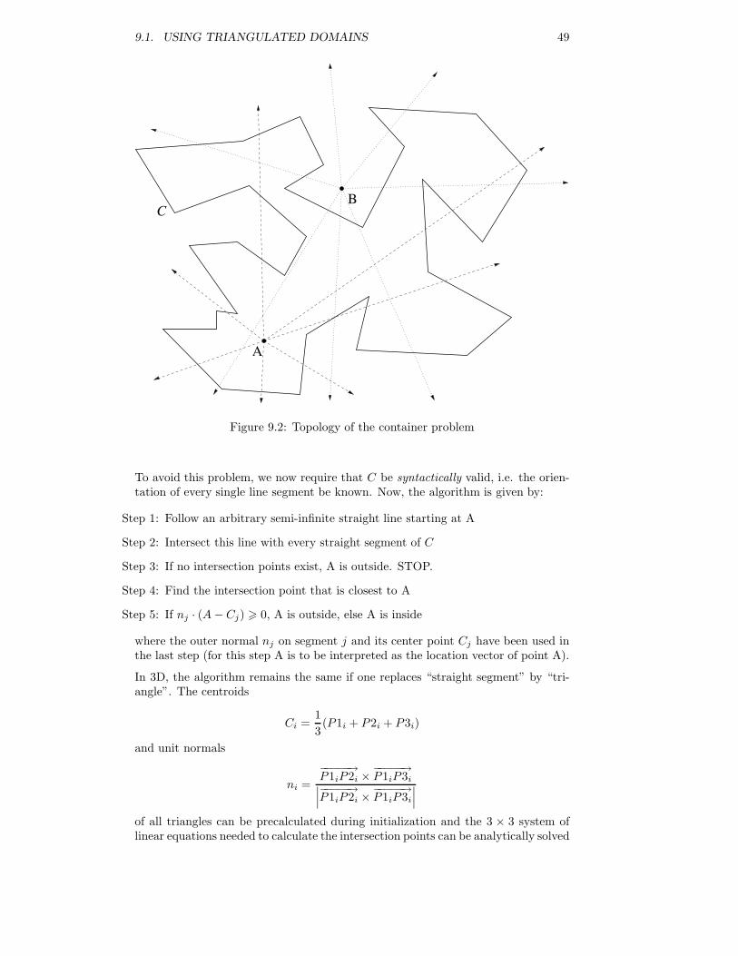
9.1. USING TRIANGULATED DOMAINS 49
B
A
C
Figure 9.2: Topology of the container problem
To avoid this problem, we now require that C be syntactically valid, i.e. the orien-tation of every single line segment be known. Now, the algorithm is given by:
Step 1: Follow an arbitrary semi-infinite straight line starting at A
Step 2: Intersect this line with every straight segment of C
Step 3: If no intersection points exist, A is outside. STOP.
Step 4: Find the intersection point that is closest to A
Step 5: If nj · (A− Cj) 0, A is outside, else A is inside
where the outer normal nj on segment j and its center point Cj have been used inthe last step (for this step A is to be interpreted as the location vector of point A).
In 3D, the algorithm remains the same if one replaces “straight segment” by “tri-angle”. The centroids
Ci =13(P1i + P2i + P3i)
and unit normals
ni =−−−−−→P1iP2i ×
−−−−−→P1iP3i∣∣∣−−−−−→P1iP2i ×−−−−−→P1iP3i
∣∣∣of all triangles can be precalculated during initialization and the 3 × 3 system oflinear equations needed to calculate the intersection points can be analytically solved
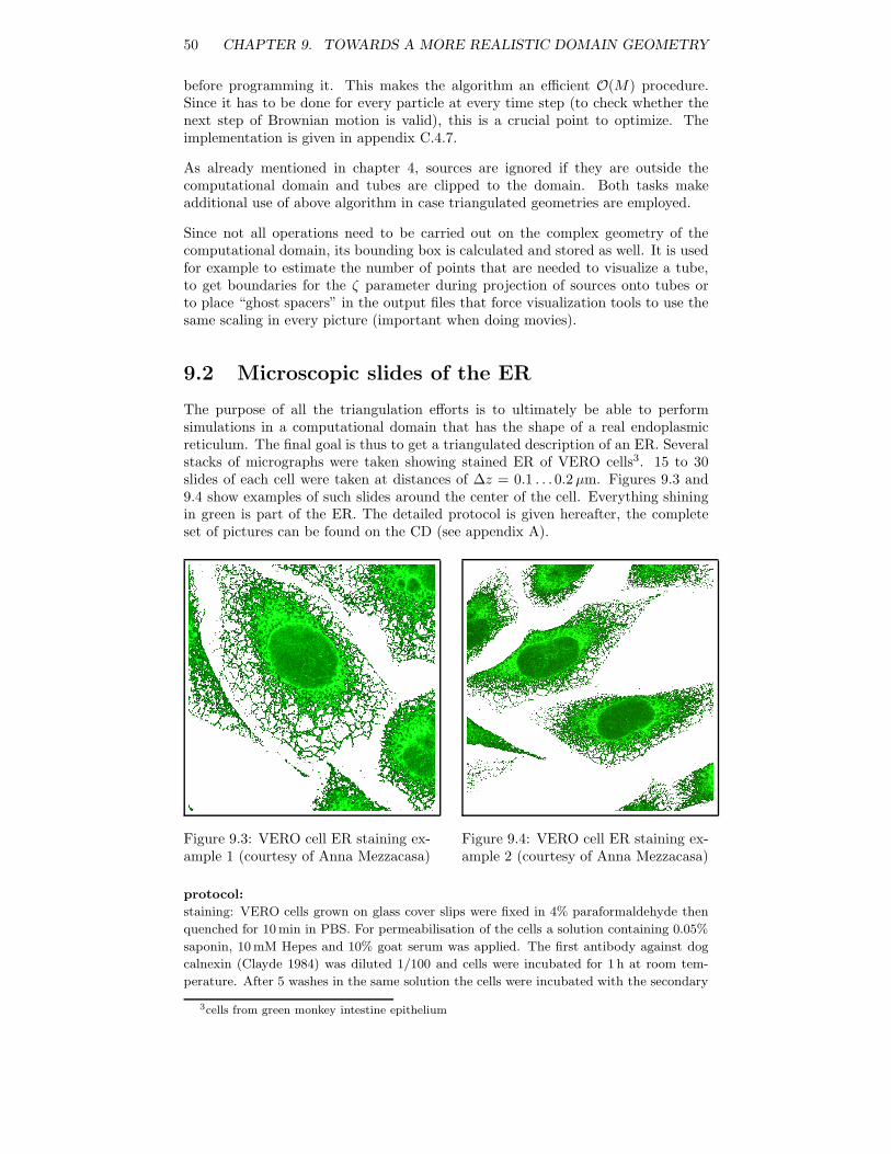
50 CHAPTER 9. TOWARDS A MORE REALISTIC DOMAIN GEOMETRY
before programming it. This makes the algorithm an efficient O(M) procedure.Since it has to be done for every particle at every time step (to check whether thenext step of Brownian motion is valid), this is a crucial point to optimize. Theimplementation is given in appendix C.4.7.
As already mentioned in chapter 4, sources are ignored if they are outside thecomputational domain and tubes are clipped to the domain. Both tasks makeadditional use of above algorithm in case triangulated geometries are employed.
Since not all operations need to be carried out on the complex geometry of thecomputational domain, its bounding box is calculated and stored as well. It is usedfor example to estimate the number of points that are needed to visualize a tube,to get boundaries for the ζ parameter during projection of sources onto tubes orto place “ghost spacers” in the output files that force visualization tools to use thesame scaling in every picture (important when doing movies).
9.2 Microscopic slides of the ER
The purpose of all the triangulation efforts is to ultimately be able to performsimulations in a computational domain that has the shape of a real endoplasmicreticulum. The final goal is thus to get a triangulated description of an ER. Severalstacks of micrographs were taken showing stained ER of VERO cells3. 15 to 30slides of each cell were taken at distances of ∆z = 0.1 . . . 0.2µm. Figures 9.3 and9.4 show examples of such slides around the center of the cell. Everything shiningin green is part of the ER. The detailed protocol is given hereafter, the completeset of pictures can be found on the CD (see appendix A).
Figure 9.3: VERO cell ER staining ex-ample 1 (courtesy of Anna Mezzacasa)
Figure 9.4: VERO cell ER staining ex-ample 2 (courtesy of Anna Mezzacasa)
protocol:
staining: VERO cells grown on glass cover slips were fixed in 4% paraformaldehyde then
quenched for 10 min in PBS. For permeabilisation of the cells a solution containing 0.05%
saponin, 10 mM Hepes and 10% goat serum was applied. The first antibody against dog
calnexin (Clayde 1984) was diluted 1/100 and cells were incubated for 1 h at room tem-
perature. After 5 washes in the same solution the cells were incubated with the secondary
3cells from green monkey intestine epithelium
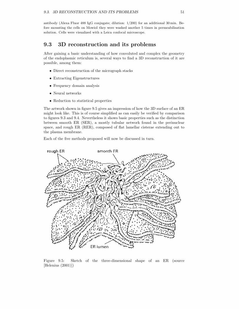
9.3. 3D RECONSTRUCTION AND ITS PROBLEMS 51
antibody (Alexa Fluor 488 IgG conjugate; dilution: 1/200) for an additional 30min. Be-
fore mounting the cells on Mowiol they were washed another 5 times in permeabilisation
solution. Cells were visualized with a Leica confocal microscope.
9.3 3D reconstruction and its problems
After gaining a basic understanding of how convoluted and complex the geometryof the endoplasmic reticulum is, several ways to find a 3D reconstruction of it arepossible, among them:
• Direct reconstruction of the micrograph stacks
• Extracting Eigenstructures
• Frequency domain analysis
• Neural networks
• Reduction to statistical properties
The artwork shown in figure 9.5 gives an impression of how the 3D surface of an ERmight look like. This is of course simplified as can easily be verified by comparisonto figures 9.3 and 9.4. Nevertheless it shows basic properties such as the distinctionbetween smooth ER (SER), a mostly tubular network found in the perinuclearspace, and rough ER (RER), composed of flat lamellar cisterae extending out tothe plasma membrane.
Each of the five methods proposed will now be discussed in turn.
Figure 9.5: Sketch of the three-dimensional shape of an ER (source[Helenius (2001)])
52 CHAPTER 9. TOWARDS A MORE REALISTIC DOMAIN GEOMETRY
9.3.1 Direct reconstruction
Direct reconstruction of a triangulated 3D surface would at least involve the follow-ing steps:
1. Thresholding of the stack micrographs to binary images having a “1” whereER is located, “0” elsewhere.
2. Outlining of the images (edge detection) to get the perimeter of the ER slide
3. Error correction to get one continuous curve without disruptions
4. Identifying corresponding structures in subsequent images (e.g. by calculatingcross-correlations)
5. Detection of corresponding curve points in subsequent slides
6. Discretizing the perimeter in each slide with a set of points
7. Connecting points on different slides (levels) to triangles
8. Error correction to make the set of triangles syntactically valid
9. Storage of point coordinates
Since it is impossible to get perfect images at arbitrarily high resolutions, therewill be errors in the slides such as “holes” in curves that should be continuous4,noise or other side effects. These can also be given raise to by the reconstructionitself, resulting in a non-coherent domain or otherwise topologically or syntacticallyinvalid sets. The number of possible errors is large making their detection andelimination very demanding. Steps 3 and 8 in above “algorithm” contain all ofthese difficulties.
Assume for a moment that the error correction problem is solved. The next pitfall isaliasing. Since digital photography introduces sampling and the slides are taken atdiscrete z levels, aliasing is a problem. The distance between two subsequent slidesis around 0.2µm, the typical distance between ER tubes or lamella is howeversmaller. According to Shannon’s theorem they can thus not be resolved in a 3Dreconstruction. Instead, one will be constructing spurious “ghost” structures givenraise to by spectral multiplication (aliasing).
Even if aliasing and error correction can be overcome using some clever algorithm,the result will be of limited use since the shape of the ER changes drastically betweendifferent individual cells and even for a given cell it changes in time as can be seen infigure 9.6. A reconstructed ER geometry would therefore only be valid for a givencell individual at a given instant in time.
Summarizing it can be said that direct reconstruction is not an option given sucha convoluted surface as the ER is.
9.3.2 Extraction of Eigenstructures
The last problem mentioned for direct reconstruction could possibly be overcome byextracting “characteristic structures” of the ER surface. This could in principle leadto a universal “ER prototype” having all the structural, statistical and geometricalproperties that make up an ER. Simulation results that are valid for all cells at
4recall that the ER consists of one continuous membrane
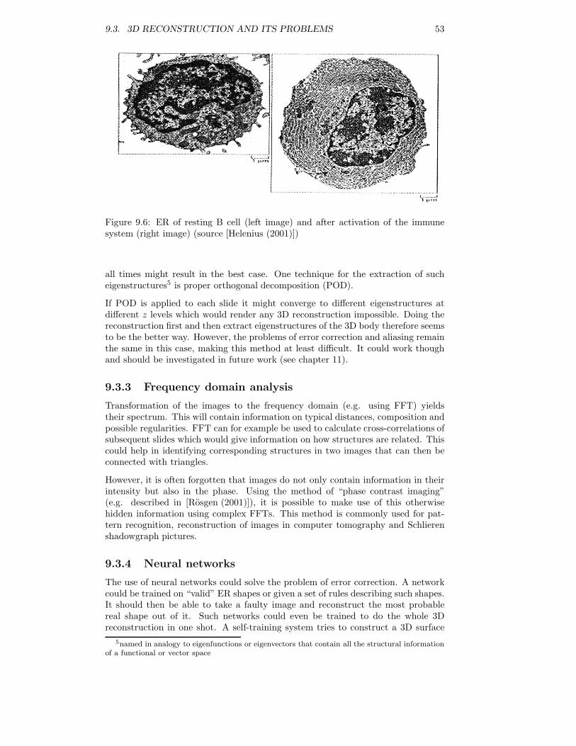
9.3. 3D RECONSTRUCTION AND ITS PROBLEMS 53
Figure 9.6: ER of resting B cell (left image) and after activation of the immunesystem (right image) (source [Helenius (2001)])
all times might result in the best case. One technique for the extraction of sucheigenstructures5 is proper orthogonal decomposition (POD).
If POD is applied to each slide it might converge to different eigenstructures atdifferent z levels which would render any 3D reconstruction impossible. Doing thereconstruction first and then extract eigenstructures of the 3D body therefore seemsto be the better way. However, the problems of error correction and aliasing remainthe same in this case, making this method at least difficult. It could work thoughand should be investigated in future work (see chapter 11).
9.3.3 Frequency domain analysis
Transformation of the images to the frequency domain (e.g. using FFT) yieldstheir spectrum. This will contain information on typical distances, composition andpossible regularities. FFT can for example be used to calculate cross-correlations ofsubsequent slides which would give information on how structures are related. Thiscould help in identifying corresponding structures in two images that can then beconnected with triangles.
However, it is often forgotten that images do not only contain information in theirintensity but also in the phase. Using the method of “phase contrast imaging”(e.g. described in [Rosgen (2001)]), it is possible to make use of this otherwisehidden information using complex FFTs. This method is commonly used for pat-tern recognition, reconstruction of images in computer tomography and Schlierenshadowgraph pictures.
9.3.4 Neural networks
The use of neural networks could solve the problem of error correction. A networkcould be trained on “valid” ER shapes or given a set of rules describing such shapes.It should then be able to take a faulty image and reconstruct the most probablereal shape out of it. Such networks could even be trained to do the whole 3Dreconstruction in one shot. A self-training system tries to construct a 3D surface
5named in analogy to eigenfunctions or eigenvectors that contain all the structural informationof a functional or vector space
54 CHAPTER 9. TOWARDS A MORE REALISTIC DOMAIN GEOMETRY
that has slides similar to those given as its input. It will continue to improve itselfaccording to some prescribed rules until a satisfactory result is obtained. Suchmethods could turn out very powerful and surely deserve attention.
9.3.5 Reduction to statistical properties
The last possible family of methods would not try to geometrically reconstructanything from the micrographs but rather use them to get some statistical data thatwill then enable one to create completely artificial shapes in the computer that canbe used as computational domains. Since they share the “defining” characteristicswith the real ER, the simulations would be universal and – most important – allproblems related to error correction and aliasing would disappear.
However, this method is far from being unproblematic or even easy. The first crucialquestion to be addressed is what statistical properties characterize the shape of theER. This has to be validated in experiments of course and then one has to thinkabout how to create artificial objects having exactly those properties. There mighteven be several different artificial shapes sharing the same defining properties (thusa non-uniquely invertible space mapping). If the chosen properties are really thedefining ones, these homologous shapes must yield the same simulation results. Ifany set of properties can be found that passes this test and yields results that arecomparable to experiments, it is likely to be the (or a) right set.
Given such a set of defining properties one could create the simplest shape possiblethat combines them and use it as a computational domain. It can now be ei-ther triangulated using standard algorithms like Delaunay triangulation or perhaps(if it can be described using closed formulas) even considered as accurate surfaceparametrization as was done for the tubes in chapter 6.1.
The following chapter will follow this road by proposing the average fractal dimen-sionality of ER shapes as their defining statistical property. Future work will haveto show whether this is true or not.
Chapter 10
Fractal properties of ERshapes
10.1 Introduction to fractal geometry
One basic problem of Euclidean geometry is its fundamental inability to describethe shape of a cloud, a mountain, a coastline, a tree or – for our purposes – anendoplasmic reticulum. Clouds are not spheres, mountains are not cones, coastlinesare not circles, bark is not smooth, nor does lightning travel in a straight line.Patterns in nature are so fragmented and irregular that they do not only exhibit ahigher degree but an altogether different level of complexity. These patterns havebeen described by Euclid as ”formless”. 20th century mathematicians have startedto investigated the morphology of the amorphous, leading to the definition of a wholenew class of shapes called fractals. Pioneering work has been done by Mandelbrot(see [Mandelbrot (1982)]) in the second half of the 20th century based on earlierwork by Hausdorff (see [Hausdorff (1919)]). Classical geometry and mathematicssimply lacked the imagination that nature has. Although structures that do notfit the theories of Euclid and Newton have been known for quite a while1, theywere regarded as ”pathological” or as ”a joke of nature”. But this pathology turnedout to be inherent in most of the familiar objects around us. Citing Blaise Pascal”L’imagination se lassera plutot de concevoir que la nature de fournir.” (imaginationtires before nature) is perhaps the best summary of this situation.
The term fractal is a neologism coined by Mandelbrot from the Latin adjectivefractus. The corresponding verb frangere means “to break, to create irregular frag-ments”. fractus therefore not only means “fragmented” (as in fraction) but also“irregular”. Fractal is the etymological opposite of algebra, which derives from theArabic word jabara = to bind together.
The geometrical class of fractal sets is characterized by certain intuitive properties,among them
• an irregular, convoluted shape
• a large or even infinite number of length scales
• statistical self-similarity (i.e. the degree of irregularity and fragmentation isidentical at all scales)
1e.g. duBois Reymond’s function (1875), Cantor’s set (around 1920) or Peano’s space-fillingcurve (1925)
55
56 CHAPTER 10. FRACTAL PROPERTIES OF ER SHAPES
Fractals can be deterministic (i.e. by complex funcion recursion) or they can alsohave stochastic irregularities as is the case for most natural shapes. Above list ishowever not a definition. The following subsections contain the thorough mathe-matical definitions in order to build a solid basis for the subsequent chapters. Thesedefinitions are however not needed to understand the rest of this report. The readermay well skip ahead to section 10.2 if not interested in theoretical considerations orthe exact definition of the term “fractal”.
10.1.1 Dimension and dimensionality
As mentioned, above list of fractal properties is not a definition of fractals. In orderto define this class of shapes, some knowledge about dimensions and outer measuresis needed.
Before 1875, dimension was defined as the minimum number of coordinates neededto span a space. However, this definition turned out to be inappropriate for thedescription of irregularity and fragmentation. Led by Cantor (1877) and Peano(1890), new definitions of dimension were introduced making the term “dimension”a loose notion. Dimension has many mathematical facets and one must never forgetthat there are several different definitions of it.
Two preliminary definitions may be useful for the following:
Definition 1. Sets for which all useful definitions of dimensions coincide are calleddimensionally concordant sets.
Definition 2. Sets for which different definitions of dimensions fail to coincide arecalled dimensionally discordant sets.
The fact that fractals are dimensionally discordant sets can be used to transformthe concept of fractals from an intuitive one to a mathematical one. In order tofinally define “fractals”, consider two different concepts of dimensionality:
• Topological dimension DT (due to Brouwer, Lebesgue, Menger and Urysohn)
• Metric dimension D (e.g. due to Hausdorff and Besicovitch)
Brouwer discovered in 1911 that the Euclidean E-Space and the Euclidean E0-Spaceare not homeomorphic2. Based on this, in 1913 he introduced an integer-valuedfunction of a space which is topologically invariant by its very definition and whichyields exactly E in the Euclidean E-Space: Each cube in Euclidean E-Space canbe decomposed into arbitrarily small bricks such that no more than E + 1 of thesebricks meet. According to Lebesgue, this number cannot be reduced any further,meaning that for any decomposition in sufficiently small bricks there must be apoint in common for at least E+1 of the bricks. The topological property E of theEuclidean E-Space (hence its name) is defined to be its topological dimension. Thisnotion of dimension coincides with our daily intuitive notion for a large number ofspaces.
In contrast to above definition, all possible concepts of fractal dimension are metricdimensions (so called outer measures) and not topological properties of a space.It involves a metric space Ω (that is a space in which the distance between twopoints is defined suitably). The different definitions of fractal dimension e.g. byCantor and Minkowski, Bouligand, Pontrjagin and Schnirelman, Kolmogorov and
2i.e. no topologically invariant transformation (one-to-one and continuous) exists that maps Eto E0
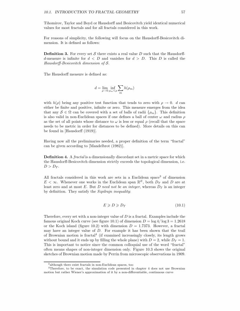
10.1. INTRODUCTION TO FRACTAL GEOMETRY 57
Tihomirov, Taylor and Boyd or Hausdorff and Besicovitch yield identical numericalvalues for most fractals and for all fractals considered in this work.
For reasons of simplicity, the following will focus on the Hausdorff-Besicovitch di-mension. It is defined as follows:
Definition 3. For every set S there exists a real value D such that the Hausdorff-d-measure is infinite for d < D and vanishes for d > D. This D is called theHausdorff-Besicovitch dimension of S.
The Hausdorff measure is defined as:
d = limρ→0
infρm<ρ
∑m
h(ρm)
with h(ρ) being any positive test function that tends to zero with ρ → 0. d caneither be finite and positive, infinite or zero. This measure emerges from the ideathat any S ∈ Ω can be covered with a set of balls of radii ρm. This definitionis also valid in non-Euclidean spaces if one defines a ball of center ω and radius ρas the set of all points whose distance to ω is less or equal ρ (recall that the spaceneeds to be metric in order for distances to be defined). More details on this canbe found in [Hausdorff (1919)].
Having now all the preliminaries needed, a proper definition of the term “fractal”can be given according to [Mandelbrot (1982)].
Definition 4. A fractal is a dimensionally discordant set in a metric space for whichthe Hausdorff-Besicovitch dimension strictly exceeds the topological dimension, i.e.D > DT .
All fractals considered in this work are sets in a Euclidean space3 of dimensionE < ∞. Whenever one works in the Euclidean span R
E , both DT and D are atleast zero and at most E. But D need not be an integer, whereas DT is an integerby definition. They satisfy the Szpilrajn inequality:
E D DT (10.1)
Therefore, every set with a non-integer value of D is a fractal. Examples include thefamous original Koch curve (see figure 10.1) of dimension D = log 4/ log 3 = 1.2618or the Koch island (figure 10.2) with dimension D = 1.7373. However, a fractalmay have an integer value of D. For example it has been shown that the trailof Brownian motion is fractal4 (if examined increasingly closely, its length growswithout bound and it ends up by filling the whole plane) with D = 2, while DT = 1.This is important to notice since the common colloquial use of the word “fractal”often means shapes of non-integer dimension only. Figure 10.3 shows the originalsketches of Brownian motion made by Perrin from microscopic observations in 1909.
3although there exist fractals in non-Euclidean spaces, too4Therefore, to be exact, the simulation code presented in chapter 4 does not use Brownian
motion but rather Wiener’s approximation of it by a non-differentiable, continuous curve
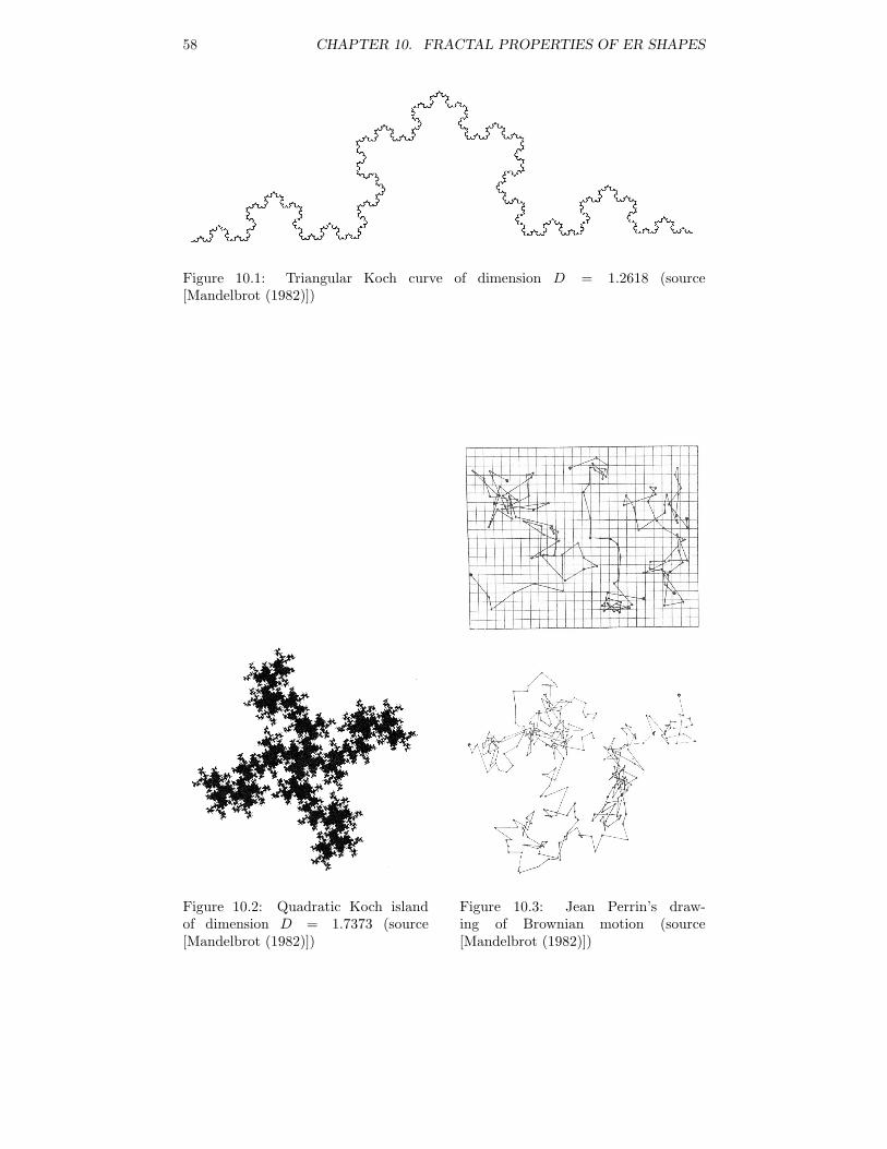
58 CHAPTER 10. FRACTAL PROPERTIES OF ER SHAPES
Figure 10.1: Triangular Koch curve of dimension D = 1.2618 (source[Mandelbrot (1982)])
Figure 10.2: Quadratic Koch islandof dimension D = 1.7373 (source[Mandelbrot (1982)])
Figure 10.3: Jean Perrin’s draw-ing of Brownian motion (source[Mandelbrot (1982)])
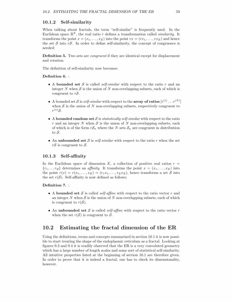
10.2. ESTIMATING THE FRACTAL DIMENSION OF THE ER 59
10.1.2 Self-similarity
When talking about fractals, the term “self-similar” is frequently used. In theEuclidean space R
E , the real ratio r defines a transformation called similarity. Ittransforms the point x = (x1, . . . , xE) into the point rx = (rx1, . . . , rxE) and hencethe set S into rS. In order to define self-similarity, the concept of congruence isneeded:
Definition 5. Two sets are congruent if they are identical except for displacementand rotation.
The definition of self-similarity now becomes:
Definition 6. :
• A bounded set S is called self-similar with respect to the ratio r and aninteger N when S is the union of N non-overlapping subsets, each of which iscongruent to rS.
• A bounded set S is self-similar with respect to the array of ratios [r(1) . . . r(N)]when S is the union of N non-overlapping subsets, respectively congruent tor(n)S.
• A bounded random set S is statistically self-similar with respect to the ratior and an integer N when S is the union of N non-overlapping subsets, eachof which is of the form rSn where the N sets Sn are congruent in distributionto S.
• An unbounded set S is self-similar with respect to the ratio r when the setrS is congruent to S.
10.1.3 Self-affinity
In the Euclidean space of dimension E, a collection of positive real ratios r =r1, . . . rR determines an affinity. It transforms the point x = (x1, . . . , xE) intothe point r(x) = r(x1, . . . , xE) = (r1x1, . . . , rExE), hence transforms a set S intothe set r(S). Self-affinity is now defined as follows:
Definition 7. :
• A bounded set S is called self-affine with respect to the ratio vector r andan integer N when S is the union of N non-overlapping subsets, each of whichis congruent to r(S).
• An unbounded set S is called self-affine with respect to the ratio vector rwhen the set r(S) is congruent to S.
10.2 Estimating the fractal dimension of the ER
Using the definitions, terms and concepts summarized in section 10.1 it is now possi-ble to start treating the shape of the endoplasmic reticulum as a fractal. Looking atfigures 9.3 and 9.4 it is readily observed that the ER is a very convoluted geometrywhich has a large number of length scales and some sort of statistical self-similarity.All intuitive properties listed at the beginning of section 10.1 are therefore given.In order to prove that it is indeed a fractal, one has to check its dimensionality,however.
60 CHAPTER 10. FRACTAL PROPERTIES OF ER SHAPES
To get a statistical average, the fractal dimension of 6 different pictures of stainedER is measured using the “resolution division algorithm” of image processing. Inprinciple, this algorithm yields an estimate for the Pontrjagin-Kolmogorov dimen-sion:
D = lim infρ→0
logN(ρ)log 1/ρ
(10.2)
As stated in section 10.1.1, all definitions of fractal dimension yield the same numer-ical values as long as the fractal is considered in a Euclidean space, which is alwaysthe case here. Therefore, this algorithm is taken for simplicity (the Hausdorff-Besicovitch dimension is hard to evaluate from its definition). In above formula, ρdenotes the radius of the balls that are used to cover the set S in the metric space Ω.Among all possible collections, the one with the smallest number of balls is chosen.If S is bounded, this number is finite and can be denoted by N(ρ).
Since the images we are dealing with are of finite resolution, ρ will not go to zerobut to the smallest measure possible, which is one pixel at full image resolution. Itis then increased by a factor of two several times. The negative slope of the linelog2N(ρ) vs. M (where ρ is 2M · ρ0) is then a good estimate for D. Thus thealgorithm proceeds as follows:
Step 1: Read image from file and take its intensity channel: I
Step 2: Normalize the image: I = (I − Imin)/(Imax − Imin)
Step 3: Threshold the image: I = 1 if I > threshold, else 0
Step 4: Outline the image
Step 5: Calculate the length of the outline at current resolution: N(ρ)
Step 6: Do a 2D convolution for discrete 2 by 2 low-pass filtering
Step 7: Reduce the image resolution by taking every second column and row of pixels:I = I(1 : 2 : N, 1 : 2 : M)
Step 8: If the edge length of the image is larger than 16 pixels, go to Step 2
Step 9: Do a linear least squares fit of log2N vs. the reduction step number to getthe dimension D
After the original (8 bit unsigned integer) image has been read from a file (digitalphotograph from the microscope, see figure 10.4), its intensity channel is calculated,converted to double precision numbers and extracted (see figure 10.5). The nor-malization step 2 is then needed to cause the algorithm to use the whole doubleprecision value space of the image. This accounts for dark or bright images thatwould otherwise yield different results. Normalization therefore makes sure thatthe results of different images will be comparable. The threshold operator thenselects all regions of the image that are brighter than a certain number between 0(black) and 1 (white). Figure 10.6 shows an example of the resulting binary imageproduced with threshold 0.05. The next operation outlines the perimeter of thehighlighted area by closed lines of pixels (see figure 10.7). The length of this line isthen measured by counting the number of pixels it contains. This value is N(ρ) inequation 10.2 where ρ is the current length scale (i.e. one pixel).
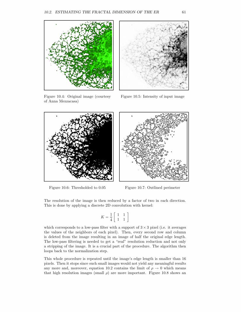
10.2. ESTIMATING THE FRACTAL DIMENSION OF THE ER 61
Figure 10.4: Original image (courtesyof Anna Mezzacasa)
Figure 10.5: Intensity of input image
Figure 10.6: Thresholded to 0.05 Figure 10.7: Outlined perimeter
The resolution of the image is then reduced by a factor of two in each direction.This is done by applying a discrete 2D convolution with kernel:
K =14
[1 11 1
]
which corresponds to a low-pass filter with a support of 3× 3 pixel (i.e. it averagesthe values of the neighbors of each pixel). Then, every second row and columnis deleted from the image resulting in an image of half the original edge length.The low-pass filtering is needed to get a “real” resolution reduction and not onlya stripping of the image. It is a crucial part of the procedure. The algorithm thenloops back to the normalization step.
This whole procedure is repeated until the image’s edge length is smaller than 16pixels. Then it stops since such small images would not yield any meaningful resultsany more and, moreover, equation 10.2 contains the limit of ρ → 0 which meansthat high resolution images (small ρ) are more important. Figure 10.8 shows an
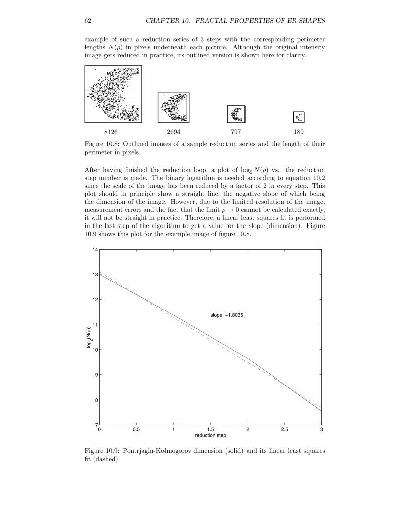
62 CHAPTER 10. FRACTAL PROPERTIES OF ER SHAPES
example of such a reduction series of 3 steps with the corresponding perimeterlengths N(ρ) in pixels underneath each picture. Although the original intensityimage gets reduced in practice, its outlined version is shown here for clarity.
8126 2694 797 189
Figure 10.8: Outlined images of a sample reduction series and the length of theirperimeter in pixels
After having finished the reduction loop, a plot of log2N(ρ) vs. the reductionstep number is made. The binary logarithm is needed according to equation 10.2since the scale of the image has been reduced by a factor of 2 in every step. Thisplot should in principle show a straight line, the negative slope of which beingthe dimension of the image. However, due to the limited resolution of the image,measurement errors and the fact that the limit ρ→ 0 cannot be calculated exactly,it will not be straight in practice. Therefore, a linear least squares fit is performedin the last step of the algorithm to get a value for the slope (dimension). Figure10.9 shows this plot for the example image of figure 10.8.
0 0.5 1 1.5 2 2.5 37
8
9
10
11
12
13
14
slope: −1.8035
reduction step
log 2(N
(ρ))
Figure 10.9: Pontrjagin-Kolmogorov dimension (solid) and its linear least squaresfit (dashed)
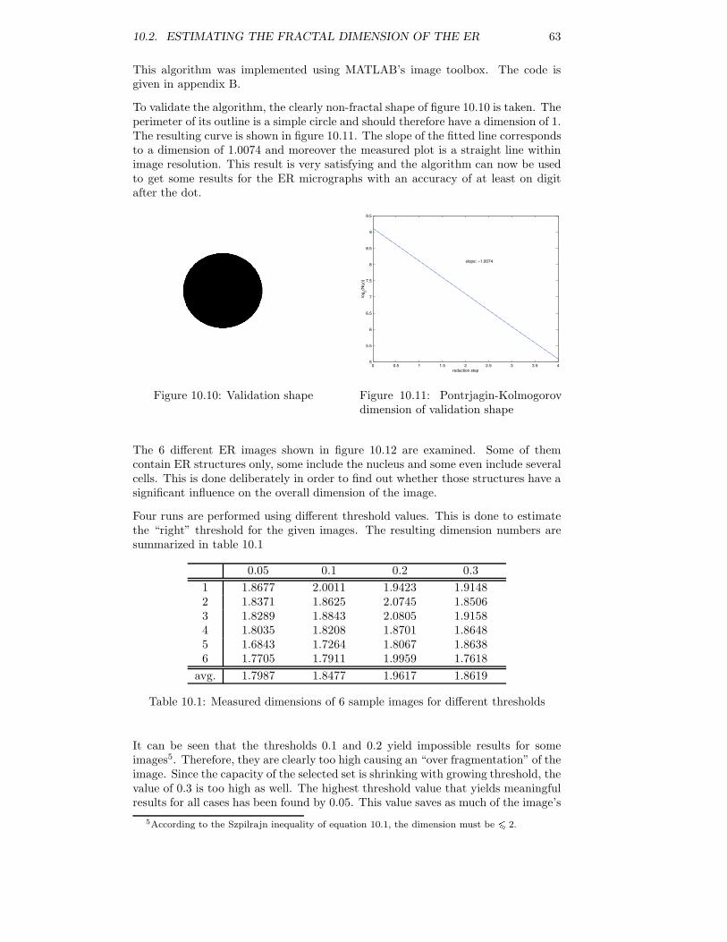
10.2. ESTIMATING THE FRACTAL DIMENSION OF THE ER 63
This algorithm was implemented using MATLAB’s image toolbox. The code isgiven in appendix B.
To validate the algorithm, the clearly non-fractal shape of figure 10.10 is taken. Theperimeter of its outline is a simple circle and should therefore have a dimension of 1.The resulting curve is shown in figure 10.11. The slope of the fitted line correspondsto a dimension of 1.0074 and moreover the measured plot is a straight line withinimage resolution. This result is very satisfying and the algorithm can now be usedto get some results for the ER micrographs with an accuracy of at least on digitafter the dot.
Figure 10.10: Validation shape
0 0.5 1 1.5 2 2.5 3 3.5 45
5.5
6
6.5
7
7.5
8
8.5
9
9.5
slope: −1.0074
reduction step
log 2(N
(ρ))
Figure 10.11: Pontrjagin-Kolmogorovdimension of validation shape
The 6 different ER images shown in figure 10.12 are examined. Some of themcontain ER structures only, some include the nucleus and some even include severalcells. This is done deliberately in order to find out whether those structures have asignificant influence on the overall dimension of the image.
Four runs are performed using different threshold values. This is done to estimatethe “right” threshold for the given images. The resulting dimension numbers aresummarized in table 10.1
0.05 0.1 0.2 0.31 1.8677 2.0011 1.9423 1.91482 1.8371 1.8625 2.0745 1.85063 1.8289 1.8843 2.0805 1.91584 1.8035 1.8208 1.8701 1.86485 1.6843 1.7264 1.8067 1.86386 1.7705 1.7911 1.9959 1.7618
avg. 1.7987 1.8477 1.9617 1.8619
Table 10.1: Measured dimensions of 6 sample images for different thresholds
It can be seen that the thresholds 0.1 and 0.2 yield impossible results for someimages5. Therefore, they are clearly too high causing an “over fragmentation” of theimage. Since the capacity of the selected set is shrinking with growing threshold, thevalue of 0.3 is too high as well. The highest threshold value that yields meaningfulresults for all cases has been found by 0.05. This value saves as much of the image’s
5According to the Szpilrajn inequality of equation 10.1, the dimension must be 2.
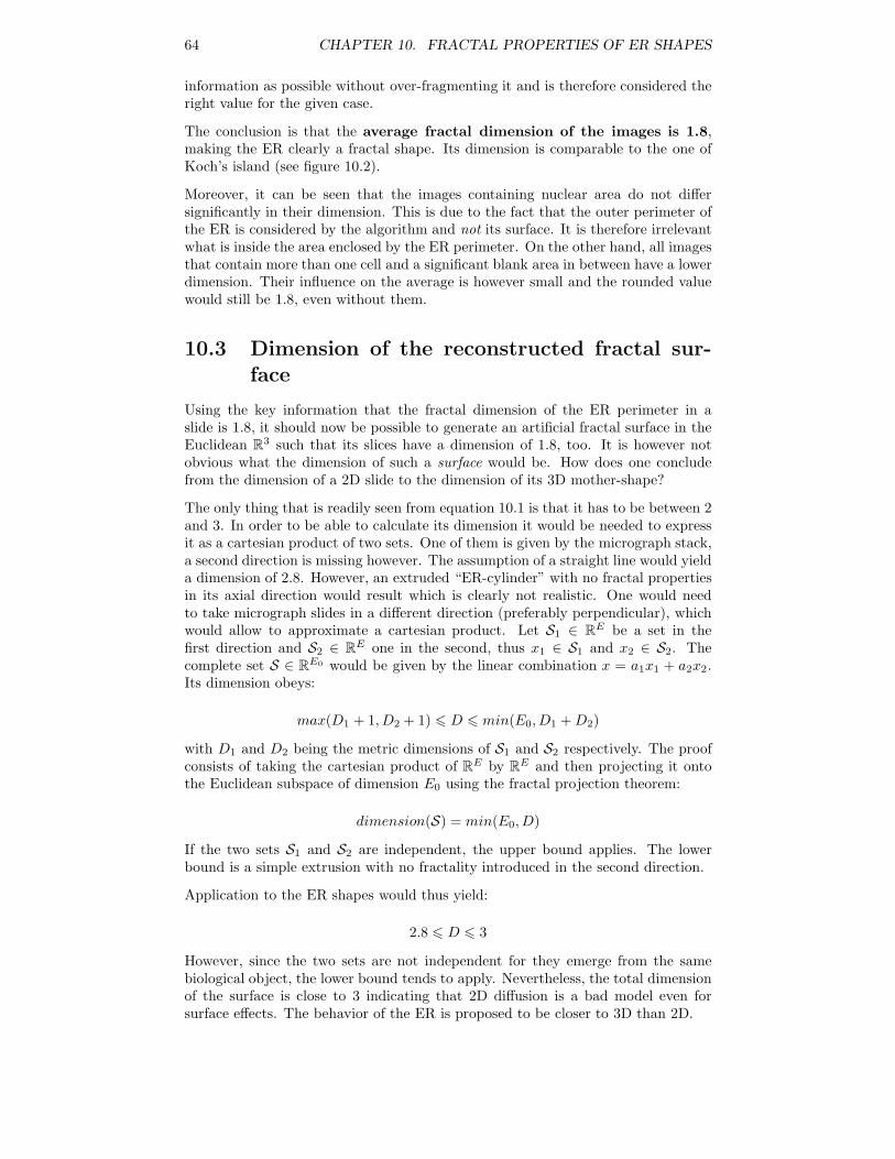
64 CHAPTER 10. FRACTAL PROPERTIES OF ER SHAPES
information as possible without over-fragmenting it and is therefore considered theright value for the given case.
The conclusion is that the average fractal dimension of the images is 1.8,making the ER clearly a fractal shape. Its dimension is comparable to the one ofKoch’s island (see figure 10.2).
Moreover, it can be seen that the images containing nuclear area do not differsignificantly in their dimension. This is due to the fact that the outer perimeter ofthe ER is considered by the algorithm and not its surface. It is therefore irrelevantwhat is inside the area enclosed by the ER perimeter. On the other hand, all imagesthat contain more than one cell and a significant blank area in between have a lowerdimension. Their influence on the average is however small and the rounded valuewould still be 1.8, even without them.
10.3 Dimension of the reconstructed fractal sur-face
Using the key information that the fractal dimension of the ER perimeter in aslide is 1.8, it should now be possible to generate an artificial fractal surface in theEuclidean R
3 such that its slices have a dimension of 1.8, too. It is however notobvious what the dimension of such a surface would be. How does one concludefrom the dimension of a 2D slide to the dimension of its 3D mother-shape?
The only thing that is readily seen from equation 10.1 is that it has to be between 2and 3. In order to be able to calculate its dimension it would be needed to expressit as a cartesian product of two sets. One of them is given by the micrograph stack,a second direction is missing however. The assumption of a straight line would yielda dimension of 2.8. However, an extruded “ER-cylinder” with no fractal propertiesin its axial direction would result which is clearly not realistic. One would needto take micrograph slides in a different direction (preferably perpendicular), whichwould allow to approximate a cartesian product. Let S1 ∈ R
E be a set in thefirst direction and S2 ∈ R
E one in the second, thus x1 ∈ S1 and x2 ∈ S2. Thecomplete set S ∈ R
E0 would be given by the linear combination x = a1x1 + a2x2.Its dimension obeys:
max(D1 + 1, D2 + 1) D min(E0, D1 +D2)
with D1 and D2 being the metric dimensions of S1 and S2 respectively. The proofconsists of taking the cartesian product of R
E by RE and then projecting it onto
the Euclidean subspace of dimension E0 using the fractal projection theorem:
dimension(S) = min(E0, D)
If the two sets S1 and S2 are independent, the upper bound applies. The lowerbound is a simple extrusion with no fractality introduced in the second direction.
Application to the ER shapes would thus yield:
2.8 D 3
However, since the two sets are not independent for they emerge from the samebiological object, the lower bound tends to apply. Nevertheless, the total dimensionof the surface is close to 3 indicating that 2D diffusion is a bad model even forsurface effects. The behavior of the ER is proposed to be closer to 3D than 2D.
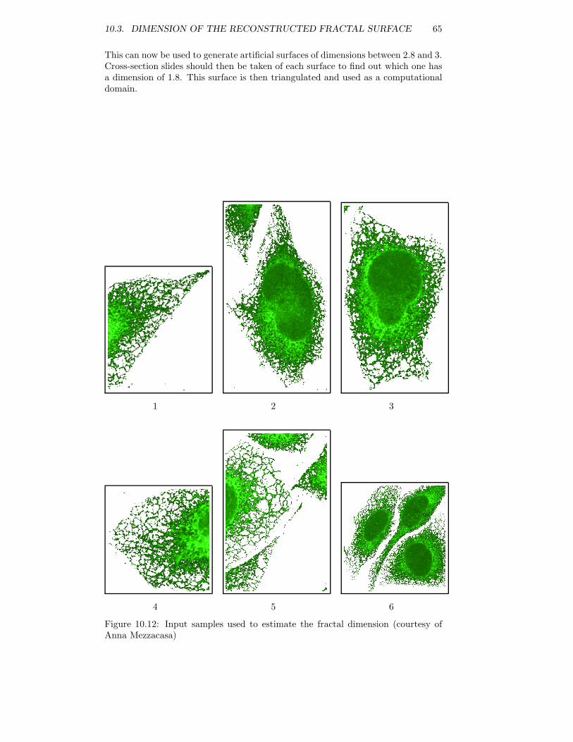
10.3. DIMENSION OF THE RECONSTRUCTED FRACTAL SURFACE 65
This can now be used to generate artificial surfaces of dimensions between 2.8 and 3.Cross-section slides should then be taken of each surface to find out which one hasa dimension of 1.8. This surface is then triangulated and used as a computationaldomain.
1 2 3
4 5 6
Figure 10.12: Input samples used to estimate the fractal dimension (courtesy ofAnna Mezzacasa)

66 CHAPTER 10. FRACTAL PROPERTIES OF ER SHAPES
Chapter 11
Conclusions and future work
In this project we started developing a computational model for protein diffusion inthe ER lumen as well as on the ER membrane. The simulation code that has beenwritten is based on 3D random walk of individual particles and handles arbitrarytriangulated geometries, sources, sinks, separator planes, tubes, anisotropy andspatial dependences of the diffusion constant. Compared to the lattice-based 2Drandom walk code by [Gheber & Edidin (1999)], this greatly improves on flexibilityand allows for new types of simulations. The usage of random walk has beeninvestigated intensively in section 4.1 and it has been shown that diffusion consistsof random walk under some assumptions that are needed to derive the diffusionequation. The usage of the simulation code is not limited to protein diffusion inthe ER but it can be seen as a computational framework for all sorts of cell-relatedsimulations such as the movement of particles along microtubules or the simulationof membrane organization.
In chapter 5 the code has been used to simulate space diffusion in 2D and 3D whichled to the conclusion that the 2D models constantly underestimate the diffusivityfrom a given measured FRAP curve. The fact that this effect seems to be inde-pendent of the number of particles and the domain geometry indicates that the 2Dmodel fundamentally fails to capture real, i.e. 3D, phenomena.
Simulations on tube surfaces in section 6.5 have shown that the FRAP resultsdepend on the tilting angle of the tube (i.e. the observation direction) in a nonlinearway. Moreover, the results are not identical to 2D results indicating a failure of the2D model to account for non-planar effects in 3D (although the diffusion on thetube surfaces is 2D in local coordinates).
The combination of surface and space diffusion in a domain of spatially varyingdiffusion constant revealed the fact that FRAP analysis cannot recover variationsinD along the axis of observation (c.f. chapter 8). This means that one should avoidhaving a bleached box that extends over heterogeneous areas of different diffusivities(e.g. different organelles).
In chapter 9, the basis for simulations in more realistic geometries has been built.As stated in section 3.4, it is the ultimate goal to isolate a reference geometry forER that can then be used to create computational models to connect FRAP curvesto D values. Topological problems have been addressed and corresponding algo-rithms were implemented. The problem of 3D surface reconstruction from stacks ofmicrographs has been addressed and different strategies and issues considered.
One possible idea of how to extract relevant statistical geometry information hasbeen proposed using the fractal dimension of the ER. Section 10.1 summarizedimportant points of fractal theory and provided thorough mathematical treatment of
67
68 CHAPTER 11. CONCLUSIONS AND FUTURE WORK
the term “dimension” as well as some important definitions. The fractal dimensionof the perimeter of ER slides has been measured using an algorithm describedand tested in section 10.2. It is around 1.8 which is clearly larger than 1, thusmaking the ER a fractal shape. It has then been estimated (using a projectiontheorem) that the total dimension of the ER surface in space is between 2.8 and3, thus making even surface diffusion a “3D-like” process that cannot be capturedusing a 2D model. It has already been pointed out by [Reits & Neefjes (2001)] thatmembrane topology (and its metric dimension is a topological property) plays animportant role in quantitative FRAP analysis. Current models described in section3.3.1 fail to account for this.
Following this ideas further, a lot of questions emerge that could unfortunately notbe addressed due to time resource limitations. They include:
• Model of chaperone binding using “sticky” tubes.
• Generation of fractal surfaces of 2.8 D 3 and validation of their dimensionby checking that their cross-sections have D ≈ 1.8
• Simulation of FRAP in artificial fractal domains
• Investigation whether different fractal domains of the same dimension yielddifferent results or not
• Validation: is fractal dimensionality the characteristic (statistical) structuralproperty of the ER ?
• Mathematical treatment of the solution of the diffusion equation in fractaldomains
• Comparison of fractal simulations to experiments
Besides this “fractal road”, other possibilities deserve attention as well, among them:
• Proper orthogonal decomposition of micrographs to extract typical structuresthat can then be reconstructed in 3D.
• Fast Fourier Transformations of micrographs and frequency domain analysis
• 3D reconstruction using (self-training) neural networks
Altogether, there is still a large number of interesting, unsolved issues that areworth being considered. This work could not be more than an introduction, acollection of basic techniques and considerations that may constitute the basis forfuture investigations. However, the hope remains that they might turn out usefulfor the work to come.
Bibliography
[Alberts et al. (1997)] Alberts, B., Bray, D., Johnson, A., Lewis, J., Raff,
M., Roberts, K. & Walter, P., 1997, Essential Cell Biology, Garlandpublishing, Inc., New York.
[Cottet & Koumoutsakos (2000)] Cottet, G.-H. & Koumoutsakos, P. D.,2000, Vortex Methods - Theory and Practice, Cambridge University Press.
[Dayel, Hom & Verkman (1999)] Dayel, M. J., Hom, E. F. Y. & Verkman, A.
S., 1999, Diffusion of Green Fluorescent Protein in the Aqueous-Phase Lumenof the Endoplasmic Reticulum, Biophysical Journal, Vol. 76, 2843-2851.
[Gheber & Edidin (1999)] Gheber, L. A. & Edidin, M., 1999, A Model for Mem-brane Patchiness: Lateral Diffusion in the Presence of Barriers and VesicleTraffic, Biophysical Journal, Vol. 77, Dec. 1999, 3163-3175.
[Hausdorff (1919)] Hausdorff, F., 1919, Dimension und ausseres Mass, Mathe-matische Annalen, 79, 157-179.
[Helenius (2001)] Helenius, A., 2001, Lecture notes on biochemistry II, Instituteof biochemistry, ETHZ.
[Jonda (1996)] Jonda, S., 1996, Structure and function of GFP,PPS2 project, Universitat Halle, http://www.biochemtech.uni-halle.de/PPS2/projects/jonda/chromoph.htm.
[Mandelbrot (1982)] Mandelbrot, B. B., 1982, The fractal geometry of nature,W. H. Freeman and Co., San Francisco.
[Marguet et al. (1999)] Marguet, D., Spiliotis, E. T., Pentcheva, T.,
Lebowitz, M., Schneck, J. & Edidin, M., 1999, Lateral Diffusion of GFP-Tagged H2Ld Molecules and of GFP-TAP1. Reports on the Assembly andRetention of these Molecules in the Endoplasmic Reticulum, Immunity, Vol.11, Aug, 1999, 231-240.
[Nehls et al. (2000)] Nehls, S., Snapp, E. L., Cole, N. B., Zaal, K. J. M.,
Kenworthy, A. K., Roberts, T. H., Ellenberg, J., Presley, J. F.,
Siggia, E. & Lippincott-Schwartz, J., 2000, Dynamics and retention ofmisfolded proteins in native ER membranes, Nature Cell Biology, Vol. 2, May2000, 288-195.
[Numerical Recipes for Fortran 77 (1996)] Press, W. H., Teukolsky, S. A.,
Vetterling, W. T. & Flannery, B. P., 1996, Numerical Recipes in For-tran 77 - The Art of Scientific Computing, 2nd edition, Cambridge UniversityPress.
[Perrin (1906)] Perrin, J., 1906, La discontinuite de la matiere, Revue du mois,1. 323-344.
69
70 BIBLIOGRAPHY
[Reits & Neefjes (2001)] Reits, E. A. J. & Neefjes, J. J., 2001, From fixed toFRAP: measuring protein mobility and activity in living cells, Nature CellBiology, Vol. 3, June 2001, E145-E147.
[Rosgen (2001)] Rosgen, Th., 2001, Quantitative Flow Visualization, Version 1.3,lecture monograph, Institute of Fluid Dynamics, ETHZ, Jan. 18, 2001.
[Storrie et al. (1994)] Storrie, B., Pepperkok, R., Stelzer, E. H. K. &
Kreis, T. E., 1994, The intracellular mobility of a viral membrane glycopro-tein by confocal microscope fluorescence recovery after photobleaching, Journalof Cell Science, 107, 1309-1319.
[White & Stelzer (1999)] White, J. & Stelzer, E., 1999, Photobleaching GFPreveals protein dynamics inside live cells, Trends in Cell Biology, Vol. 9, Feb.1999, 61-65.
[Yang, Moss & Phillips (1997)] Yang, F., Moss, L. G. & Phillips, G. N., Jr.,1997, The Molecular Structure of Green Fluorescent Protein, Dept. of biochem-istry and cell biology, Rice University, Houston, TX.
Appendix A
Contents of the companionCD-ROM
All data files that have been produced in digital form during this semester projectare contained on the attached CD-ROM.
The CD contains this report (source texts and final PS and PDF versions as wellas all pictures), all FORTRAN and MATLAB source code files, shell scripts andperl scripts, some movies and the PowerPoint presentations of the work. Moreover,all original micrographs and scans are included as well as output files of the runspresented in this report. Finally, the CD also contains some PDF files of 3rd partypapers that are related to this work as well as an EXCEL sheet containing somereal measurement data.
71
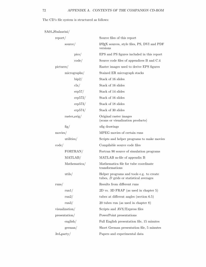
72 APPENDIX A. CONTENTS OF THE COMPANION CD-ROM
The CD’s file system is structured as follows:
SA01 Sbalzarini/
report/ Source files of this report
source/ LATEX sources, style files, PS, DVI and PDFversions
pics/ EPS and PS figures included in this report
code/ Source code files of appendices B and C.4
pictures/ Raster images used to derive EPS figures
micrographs/ Stained ER micrograph stacks
bip2/ Stack of 16 slides
clx/ Stack of 16 slides
erp57/ Stack of 14 slides
erp572/ Stack of 16 slides
erp573/ Stack of 18 slides
erp574/ Stack of 30 slides
raster orig/ Original raster images(scans or visualization products)
fig/ xfig drawings
movies/ MPEG movies of certain runs
utilities/ Scripts and helper programs to make movies
code/ Compilable source code files
FORTRAN/ Fortran 90 source of simulation programs
MATLAB/ MATLAB m-file of appendix B
Mathematica/ Mathematica file for tube coordinatetransformations
utils/ Helper programs and tools e.g. to createtubes, D grids or statistical averages
runs/ Results from different runs
run1/ 2D vs. 3D FRAP (as used in chapter 5)
run2/ tubes at different angles (section 6.5)
run3/ 20 tubes run (as used in chapter 8)
visualization/ Scripts and AVS/Express files
presentation/ PowerPoint presentations
english/ Full English presentation file, 15 minutes
german/ Short German presentation file, 5 minutes
3rd party/ Papers and experimental data
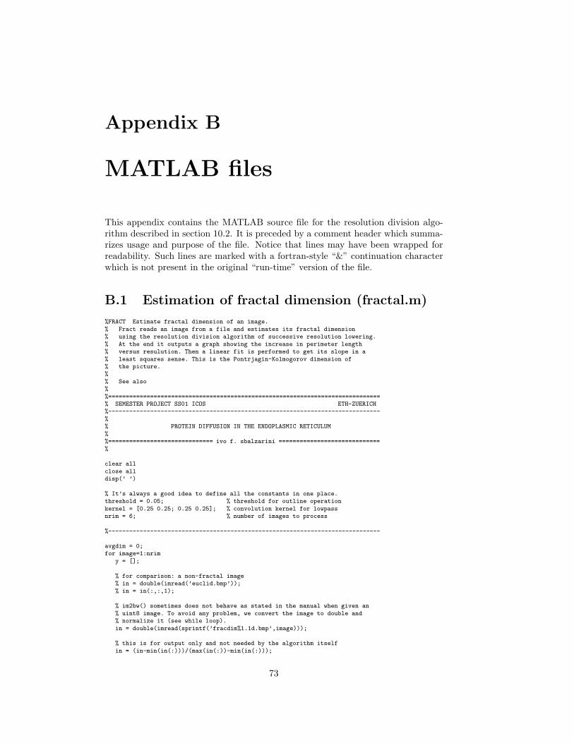
Appendix B
MATLAB files
This appendix contains the MATLAB source file for the resolution division algo-rithm described in section 10.2. It is preceded by a comment header which summa-rizes usage and purpose of the file. Notice that lines may have been wrapped forreadability. Such lines are marked with a fortran-style “&” continuation characterwhich is not present in the original “run-time” version of the file.
B.1 Estimation of fractal dimension (fractal.m)
%FRACT Estimate fractal dimension of an image.% Fract reads an image from a file and estimates its fractal dimension% using the resolution division algorithm of successive resolution lowering.% At the end it outputs a graph showing the increase in perimeter length% versus resulution. Then a linear fit is performed to get its slope in a% least squares sense. This is the Pontrjagin-Kolmogorov dimension of% the picture.%% See also%%==============================================================================% SEMESTER PROJECT SS01 ICOS ETH-ZUERICH%------------------------------------------------------------------------------%% PROTEIN DIFFUSION IN THE ENDOPLASMIC RETICULUM%%============================== ivo f. sbalzarini =============================%
clear allclose alldisp(’ ’)
% It’s always a good idea to define all the constants in one place.threshold = 0.05; % threshold for outline operationkernel = [0.25 0.25; 0.25 0.25]; % convolution kernel for lowpassnrim = 6; % number of images to process
%------------------------------------------------------------------------------
avgdim = 0;for image=1:nrim
y = [];
% for comparison: a non-fractal image% in = double(imread(’euclid.bmp’));% in = in(:,:,1);
% im2bw() sometimes does not behave as stated in the manual when given an% uint8 image. To avoid any problem, we convert the image to double and% normalize it (see while loop).in = double(imread(sprintf(’fracdim%1.1d.bmp’,image)));
% this is for output only and not needed by the algorithm itselfin = (in-min(in(:)))/(max(in(:))-min(in(:)));
73
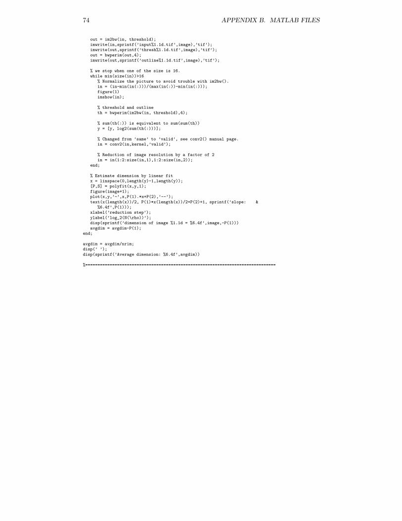
74 APPENDIX B. MATLAB FILES
out = im2bw(in, threshold);imwrite(in,sprintf(’input%1.1d.tif’,image),’tif’);imwrite(out,sprintf(’thresh%1.1d.tif’,image),’tif’);out = bwperim(out,4);imwrite(out,sprintf(’outline%1.1d.tif’,image),’tif’);
% we stop when one of the size is 16.while min(size(in))>16
% Normalize the picture to avoid trouble with im2bw().in = (in-min(in(:)))/(max(in(:))-min(in(:)));figure(1)imshow(in);
% threshold and outlineth = bwperim(im2bw(in, threshold),4);
% sum(th(:)) is equivalent to sum(sum(th))y = [y, log2(sum(th(:)))];
% Changed from ’same’ to ’valid’, see conv2() manual page.in = conv2(in,kernel,’valid’);
% Reduction of image resolution by a factor of 2in = in(1:2:size(in,1),1:2:size(in,2));
end;
% Estimate dimension by linear fitx = linspace(0,length(y)-1,length(y));[P,S] = polyfit(x,y,1);figure(image+1);plot(x,y,’-’,x,P(1).*x+P(2),’--’);text(x(length(x))/2, P(1)*x(length(x))/2+P(2)+1, sprintf(’slope: &
%6.4f’,P(1)));xlabel(’reduction step’);ylabel(’log_2(N(\rho))’);disp(sprintf(’dimension of image %1.1d = %6.4f’,image,-P(1)))avgdim = avgdim-P(1);
end;
avgdim = avgdim/nrim;disp(’ ’);disp(sprintf(’Average dimension: %6.4f’,avgdim))
%==============================================================================
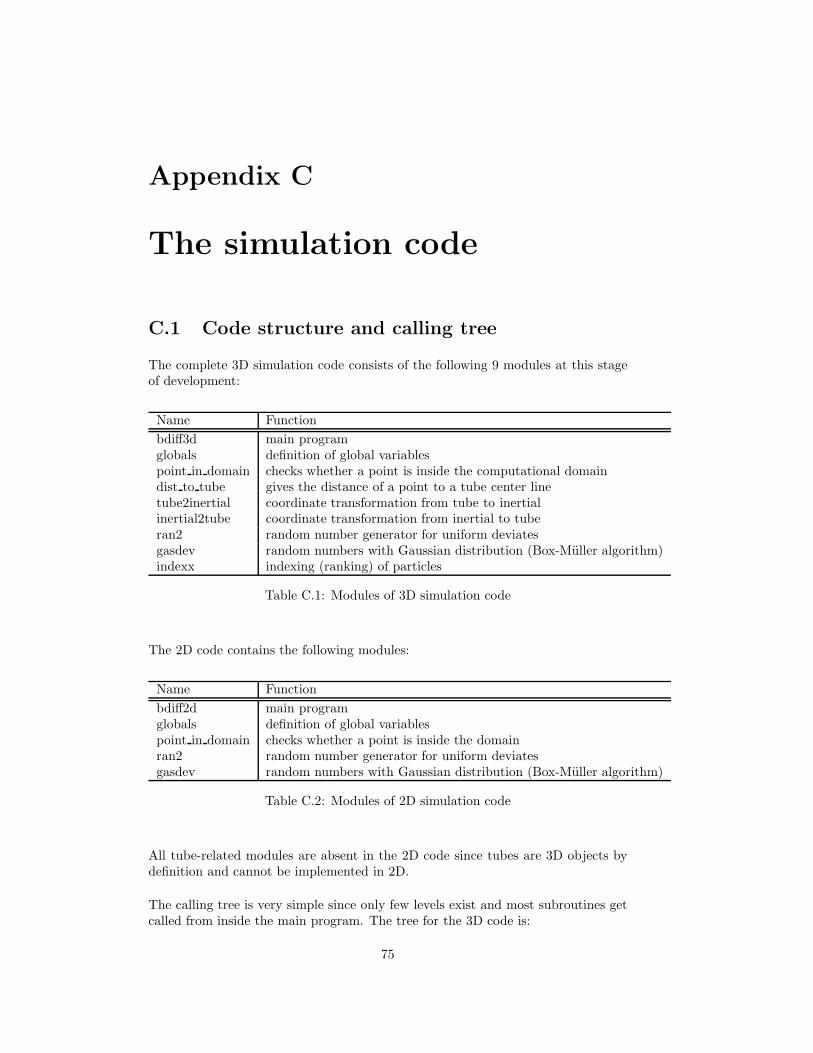
Appendix C
The simulation code
C.1 Code structure and calling tree
The complete 3D simulation code consists of the following 9 modules at this stageof development:
Name Functionbdiff3d main programglobals definition of global variablespoint in domain checks whether a point is inside the computational domaindist to tube gives the distance of a point to a tube center linetube2inertial coordinate transformation from tube to inertialinertial2tube coordinate transformation from inertial to tuberan2 random number generator for uniform deviatesgasdev random numbers with Gaussian distribution (Box-Muller algorithm)indexx indexing (ranking) of particles
Table C.1: Modules of 3D simulation code
The 2D code contains the following modules:
Name Functionbdiff2d main programglobals definition of global variablespoint in domain checks whether a point is inside the domainran2 random number generator for uniform deviatesgasdev random numbers with Gaussian distribution (Box-Muller algorithm)
Table C.2: Modules of 2D simulation code
All tube-related modules are absent in the 2D code since tubes are 3D objects bydefinition and cannot be implemented in 2D.
The calling tree is very simple since only few levels exist and most subroutines getcalled from inside the main program. The tree for the 3D code is:
75
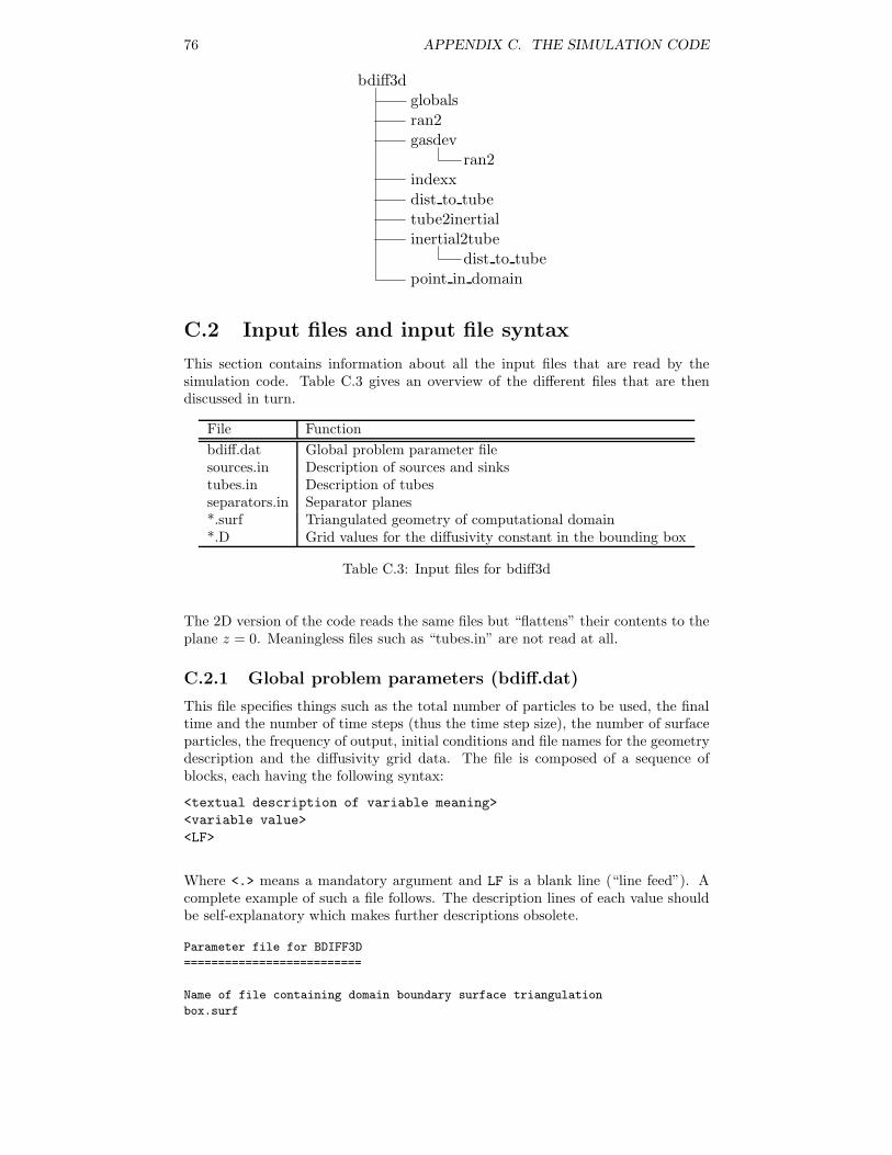
76 APPENDIX C. THE SIMULATION CODE
bdiff3dglobals
ran2gasdevran2
indexxdist to tubetube2inertialinertial2tube
dist to tubepoint in domain
C.2 Input files and input file syntax
This section contains information about all the input files that are read by thesimulation code. Table C.3 gives an overview of the different files that are thendiscussed in turn.
File Functionbdiff.dat Global problem parameter filesources.in Description of sources and sinkstubes.in Description of tubesseparators.in Separator planes*.surf Triangulated geometry of computational domain*.D Grid values for the diffusivity constant in the bounding box
Table C.3: Input files for bdiff3d
The 2D version of the code reads the same files but “flattens” their contents to theplane z = 0. Meaningless files such as “tubes.in” are not read at all.
C.2.1 Global problem parameters (bdiff.dat)
This file specifies things such as the total number of particles to be used, the finaltime and the number of time steps (thus the time step size), the number of surfaceparticles, the frequency of output, initial conditions and file names for the geometrydescription and the diffusivity grid data. The file is composed of a sequence ofblocks, each having the following syntax:
<textual description of variable meaning><variable value><LF>
Where <.> means a mandatory argument and LF is a blank line (“line feed”). Acomplete example of such a file follows. The description lines of each value shouldbe self-explanatory which makes further descriptions obsolete.
Parameter file for BDIFF3D
==========================
Name of file containing domain boundary surface triangulation
box.surf
C.2. INPUT FILES AND INPUT FILE SYNTAX 77
Name of file containing D values for the whole domain
box_uni_iso.D
Number of particles
25000
Read initial particle distribution and properties from file? 1=yes
0
Name of file containing initial particle positions and properties
part_init.in
Final time of simulation in seconds
20
Number of simulation time steps
4000
Output particle positions every ... time steps
10
number of particles that diffuse on tube surfaces only
12500
record complete trajectory path for every particle in output files ?
.FALSE.
probability for a particle to stick to tube surfaces when it hits it
0.9
probability for surface particles to be released into space again
0.2
C.2.2 Sources and sinks (sources.in)
Sources and sinks are defined by their location in inertial space (x, y, z) and strength(mean number of particles produced/swallowed per unit time). Note that the num-ber of particles in the strength is to be given per unit time and not per time step∆t. The code will then decide how many particles to process per time step in orderto reach the given number on an average. A sink is simply defined as a source ofnegative strength. The last column contains a flag (0 or 1) for each source thatdefines whether this source is on a tube surface or not. If a “1” is given but thepoint defined by (x, y, z) is not on any tube surface, it will be projected onto theclosest tube surface by the code (see section 6.4). The effective positions will beoutput in “sources.out” and “sinks.out” after initialization (see appendix C.3.1 forfurther reference). Line 5 of the file contains the number of sources to be read.If this is 0, all source definitions will be ignored. The number of lines that definesources must be at least equal to this value. Thus, the syntax is:
[5] <number of sources and sinks>[9-] <location: <x> <y> <z>> <strength> <surface flag>
The numbers in square brackets are line numbers in the file, triangular bracketscontain mandatory arguments. All other lines contain comments that are ignoredby the program. An example file could look like this (the numbers to the left are
78 APPENDIX C. THE SIMULATION CODE
line numbers and are given for reference only. They must not be included in a realfile):
1 Defines sources and sinks (negative sources)
2 ============================================
3
4 Number of sources/sinks
5 0
6
7 x y z strength [particles/time] on tube (1/0)
8 ---------------------------------------------------------------------
9 2.0 2.0 1.0 200.0 1
10 3.0 2.0 1.0 -100.0 0
11 2.5 1.0 2.67 50.0 1
C.2.3 Tubes (tubes.in)
Tubes are defined by their starting point, a direction vector and a radius according tosection 6.1. Besides this, the input file also contains the surface diffusivity coefficientand the surface permeability for each tube. The diffusivity is only valid for surfaceparticles moving on the surface of that tube. The permeability gives the probabilityat which a space particle is allowed to cross the tube surface (i.e. the tube surfacesare membranes that divide the space in “inside” and “outside”). If the permeabilityis 0, no space particles are allowed to cross that tube’s surface, if it is 1, all movesacross the surface are allowed and the tube membrane is not “felt” by space particlesat all. Line 5 contains the total number of tubes that are to be read, i.e. the codewill consider all tubes described in lines 10 to 10 + (n − 1) where n is the numbergiven in line 5. The general syntax is:
[5] <number of tubes>[10-] <direction vector: <x> <y> <z>> <start: <x> <y> <z>> &
<radius> <diffusivity> <permeability>
The continuation character “&” indicates that this is to be written on a single linein the real input file. It had to be wrapped here to fit the page. All tubes areclipped to the computational domain. Therefore, the starting point may also beoutside of the domain. A real example of a tube description file follows.
1 Defines tubes by direction vector and radius, diffusion on surface only
2 =======================================================================
3
4 nr. of tubes
5 4
6
7 direction vector starting point radius D_surf perm
8 x y z x y z
9 -------------------------------------------------------------------------------
10 1.000 0.000 0.800 0.000 0.190 0.500 0.048 0.400 0.000
11 -1.000 0.000 0.800 4.000 0.381 0.500 0.048 0.400 0.000
12 1.000 0.000 0.800 0.000 0.571 0.500 0.048 0.400 0.000
13 -1.000 0.000 0.800 4.000 0.762 0.500 0.048 0.400 0.000
C.2. INPUT FILES AND INPUT FILE SYNTAX 79
C.2.4 Separator planes (separators.in)
Separator planes can be used to subdivide the computational domain (more preciseits bounding box) into spaces separated from each other by membranes of certainpermeability. There are three classes of planes: x, y and z separators. x separatorplanes are parallel to the yz plane at a certain x coordinate, similar for y andz separators. The number of separators of each class is mentioned first, followedby the coordinates and permeabilities. See appendix C.2.3 about the definition ofpermeability that is used here. Each class of separators is defined in its own blockwhich has the general syntax:
block x, y, z<number of planes>LFLF<coordinate of plane> <permeability>...
end block
where curly brackets enclose optional arguments. The following example file definesone x separator (at x = 2.0) and two y separators (at y = 1.5 and y = 3.8) at givenpermeabilities. No z separators are defined, therefore no definition lines follow there.
1 Defines separator planes with controlled permeability
2 =====================================================
3
4 nr. of x separators
5 1
6
7 x coordinates of separator planes and permeabilities
8 2.0 0.6
9
10 nr. of y separators
11 2
12
13 y coordinates of separator planes and permeabilities
14 1.5 0.8
15 3.8 0.4
16
17 nr. of z separators
18 0
19
20 z coordinates of separator planes and permeabilities
C.2.5 Domain surface description
The computational domain in which simulations are performed is defined in a filecontaining a triangulated description of it. See section 9.1 for details on triangu-lation. The name of this input file is specified in the global parameter file (seeappendix C.2.1) and can be chosen arbitrarily. The triangulation is given as a setof triangles each described by its three vertices in inertial (x, y, z) space. The totalnumber of triangles to be read is given on line 6. The general syntax is:
[6] <number of triangles>[13-] <point 1: <x> <y> <z>> <point 2: <x> <y> <z>> <point 3: <x> <y> <z>>
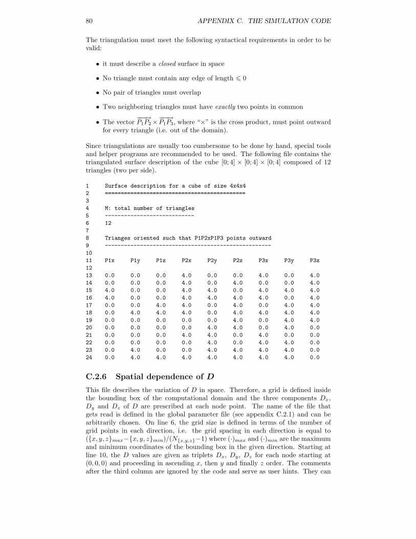
80 APPENDIX C. THE SIMULATION CODE
The triangulation must meet the following syntactical requirements in order to bevalid:
• it must describe a closed surface in space
• No triangle must contain any edge of length 0
• No pair of triangles must overlap
• Two neighboring triangles must have exactly two points in common
• The vector−−−→P1P2×
−−−→P1P3, where “×” is the cross product, must point outward
for every triangle (i.e. out of the domain).
Since triangulations are usually too cumbersome to be done by hand, special toolsand helper programs are recommended to be used. The following file contains thetriangulated surface description of the cube [0; 4] × [0; 4] × [0; 4] composed of 12triangles (two per side).
1 Surface description for a cube of size 4x4x4
2 ============================================
3
4 M: total number of triangles
5 ----------------------------
6 12
7
8 Trianges oriented such that P1P2xP1P3 points outward
9 ----------------------------------------------------
10
11 P1x P1y P1z P2x P2y P2z P3x P3y P3z
12
13 0.0 0.0 0.0 4.0 0.0 0.0 4.0 0.0 4.0
14 0.0 0.0 0.0 4.0 0.0 4.0 0.0 0.0 4.0
15 4.0 0.0 0.0 4.0 4.0 0.0 4.0 4.0 4.0
16 4.0 0.0 0.0 4.0 4.0 4.0 4.0 0.0 4.0
17 0.0 0.0 4.0 4.0 0.0 4.0 0.0 4.0 4.0
18 0.0 4.0 4.0 4.0 0.0 4.0 4.0 4.0 4.0
19 0.0 0.0 0.0 0.0 0.0 4.0 0.0 4.0 4.0
20 0.0 0.0 0.0 0.0 4.0 4.0 0.0 4.0 0.0
21 0.0 0.0 0.0 4.0 4.0 0.0 4.0 0.0 0.0
22 0.0 0.0 0.0 0.0 4.0 0.0 4.0 4.0 0.0
23 0.0 4.0 0.0 0.0 4.0 4.0 4.0 4.0 0.0
24 0.0 4.0 4.0 4.0 4.0 4.0 4.0 4.0 0.0
C.2.6 Spatial dependence of D
This file describes the variation of D in space. Therefore, a grid is defined insidethe bounding box of the computational domain and the three components Dx,Dy and Dz of D are prescribed at each node point. The name of the file thatgets read is defined in the global parameter file (see appendix C.2.1) and can bearbitrarily chosen. On line 6, the grid size is defined in terms of the number ofgrid points in each direction, i.e. the grid spacing in each direction is equal to(x, y, zmax−x, y, zmin)/(Nx,y,z−1) where (·)max and (·)min are the maximumand minimum coordinates of the bounding box in the given direction. Starting atline 10, the D values are given as triplets Dx, Dy, Dz for each node starting at(0, 0, 0) and proceeding in ascending x, then y and finally z order. The commentsafter the third column are ignored by the code and serve as user hints. They can
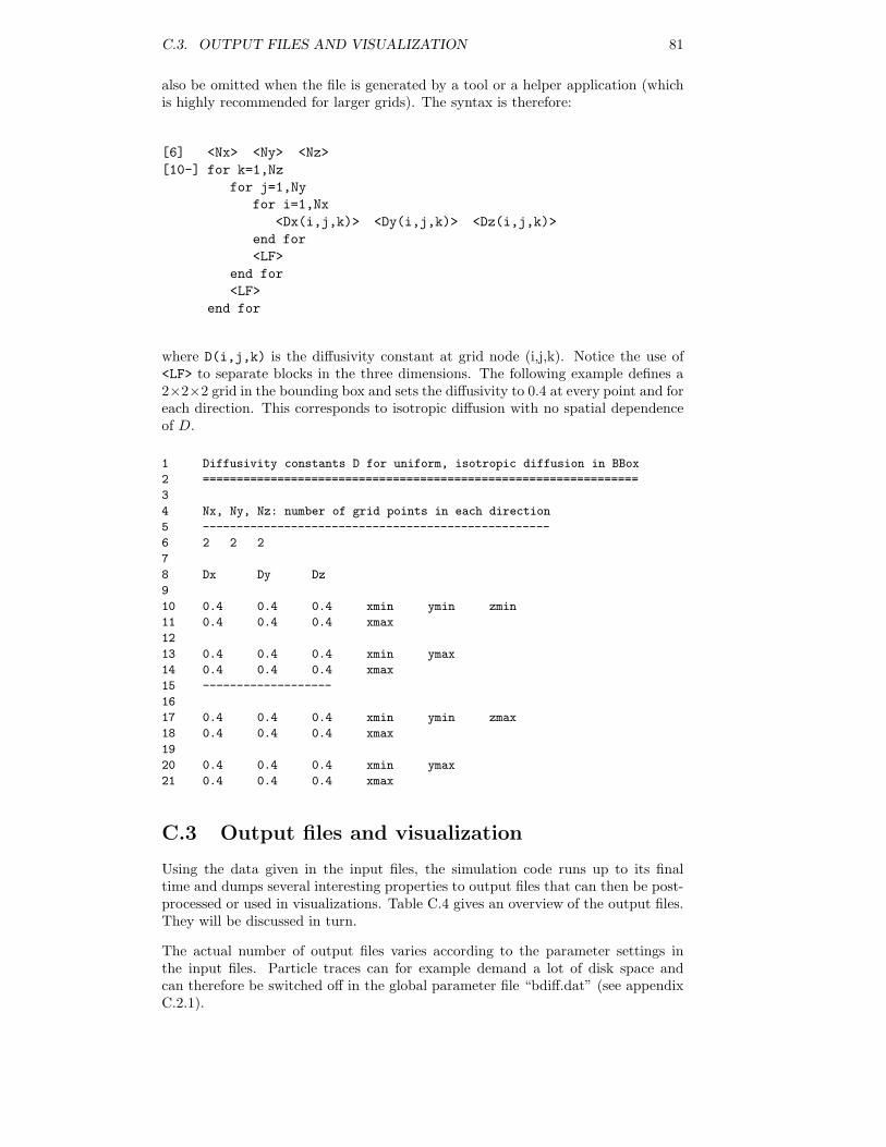
C.3. OUTPUT FILES AND VISUALIZATION 81
also be omitted when the file is generated by a tool or a helper application (whichis highly recommended for larger grids). The syntax is therefore:
[6] <Nx> <Ny> <Nz>[10-] for k=1,Nz
for j=1,Nyfor i=1,Nx
<Dx(i,j,k)> <Dy(i,j,k)> <Dz(i,j,k)>end for<LF>
end for<LF>
end for
where D(i,j,k) is the diffusivity constant at grid node (i,j,k). Notice the use of<LF> to separate blocks in the three dimensions. The following example defines a2×2×2 grid in the bounding box and sets the diffusivity to 0.4 at every point and foreach direction. This corresponds to isotropic diffusion with no spatial dependenceof D.
1 Diffusivity constants D for uniform, isotropic diffusion in BBox
2 ================================================================
3
4 Nx, Ny, Nz: number of grid points in each direction
5 ---------------------------------------------------
6 2 2 2
7
8 Dx Dy Dz
9
10 0.4 0.4 0.4 xmin ymin zmin
11 0.4 0.4 0.4 xmax
12
13 0.4 0.4 0.4 xmin ymax
14 0.4 0.4 0.4 xmax
15 -------------------
16
17 0.4 0.4 0.4 xmin ymin zmax
18 0.4 0.4 0.4 xmax
19
20 0.4 0.4 0.4 xmin ymax
21 0.4 0.4 0.4 xmax
C.3 Output files and visualization
Using the data given in the input files, the simulation code runs up to its finaltime and dumps several interesting properties to output files that can then be post-processed or used in visualizations. Table C.4 gives an overview of the output files.They will be discussed in turn.
The actual number of output files varies according to the parameter settings inthe input files. Particle traces can for example demand a lot of disk space andcan therefore be switched off in the global parameter file “bdiff.dat” (see appendixC.2.1).
82 APPENDIX C. THE SIMULATION CODE
File Functionsources.out Effective positions and strengths of sourcessinks.out Effective positions and strengths of sinkstubes.out Tubes for visualizationsurface.gnu Domain surface for visualizationsurface normals.gnu Surface normalsfluoresc.out FRAP datappos space????.out Positions of space particles at time step ????ppos surf????.out Positions of surface particles at time step ????traces surf.out Traces (streaklines) of surface particlestraces space.out Traces (streaklines) of space particlesSTDOUT Several parameters and settings
Table C.4: Possible output files of bdiff3d
C.3.1 Sources and sinks (sources.out/sinks.out)
The files “sources.out” and “sinks.out” contain positions and strengths of sourcesand sinks that have been used in a particular simulation run. According to appendixC.2.2, sources (and sinks) can be declared to be on the surface of a tube. If thepoints given in the input files do not lie on the surface of a tube (which usually isthe case), then they get projected onto the closest tube. The actual position thathas been calculated like this can be found in the output files. The syntax is thesame for both files:
<x-pos> <y-pos> <z-pos><strength>
For the example file given in appendix C.2.2, the output would for example (de-pending on the tube distribution) look like this:
sources.out:
2.226130846515382 1.959964561491936 1.282663558144227
200.0000000000000
2.532411322312637 0.6834176429403847 2.629485847109203
50.00000000000000
sinks.out:
3.000000000000000 2.000000000000000 1.000000000000000
-100.0000000000000
Besides the determination of actual positions, these files can be used to visualizesources and sinks or simply to keep record of a past run.
C.3.2 Tubes (tubes.out)
Since tube properties are not altered by the code and they are already repeated inthe terminal output (see appendix C.3.8) for records and control, this output filecontains visualization data instead. For each tube, a number of points on its surface(typically Nradial = 20 in radial direction and Naxial = 100 in axial direction) aredumped out in (x, y, z) notation if they are inside the computational domain. Thesyntax is simply:
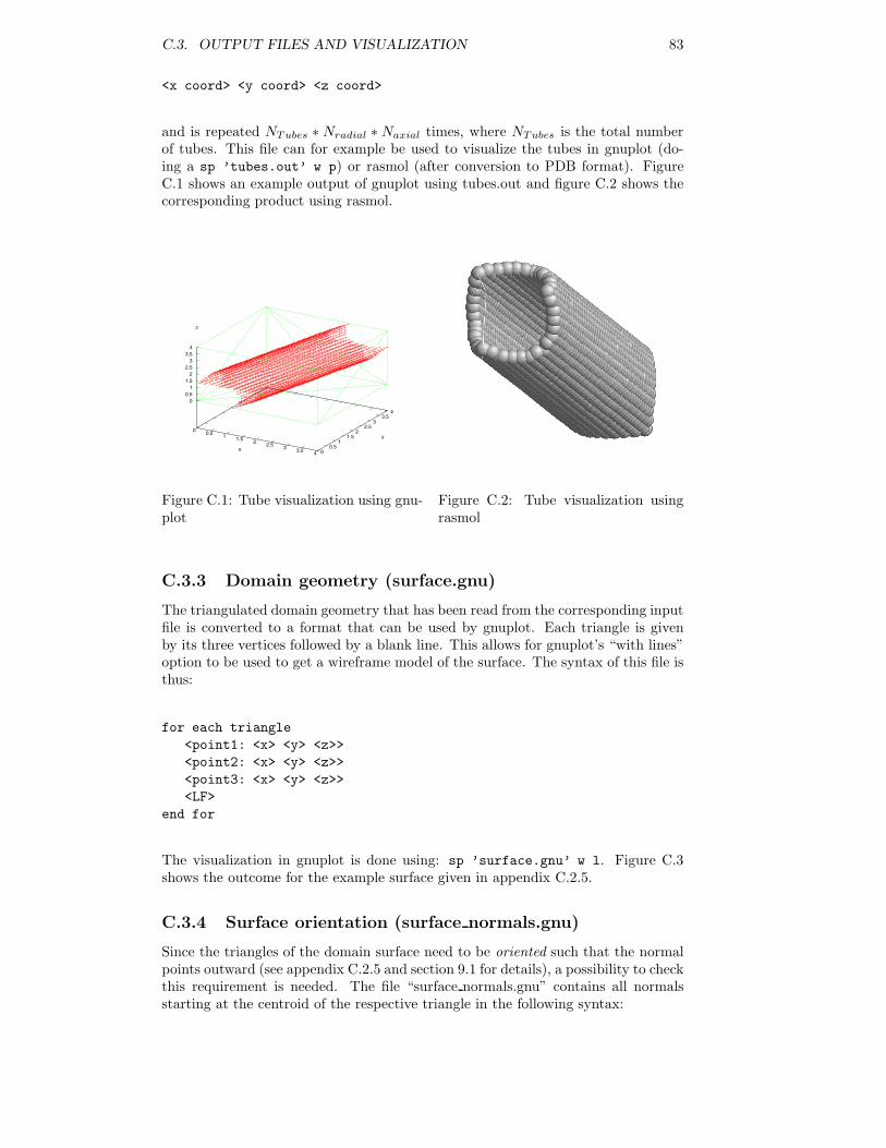
C.3. OUTPUT FILES AND VISUALIZATION 83
<x coord> <y coord> <z coord>
and is repeated NTubes ∗ Nradial ∗ Naxial times, where NTubes is the total numberof tubes. This file can for example be used to visualize the tubes in gnuplot (do-ing a sp ’tubes.out’ w p) or rasmol (after conversion to PDB format). FigureC.1 shows an example output of gnuplot using tubes.out and figure C.2 shows thecorresponding product using rasmol.
0 0.5 1 1.5 2 2.5 3 3.5 4x 0
0.51
1.52
2.53
3.54
y
00.5
11.5
22.5
33.5
4
z
Figure C.1: Tube visualization using gnu-plot
Figure C.2: Tube visualization usingrasmol
C.3.3 Domain geometry (surface.gnu)
The triangulated domain geometry that has been read from the corresponding inputfile is converted to a format that can be used by gnuplot. Each triangle is givenby its three vertices followed by a blank line. This allows for gnuplot’s “with lines”option to be used to get a wireframe model of the surface. The syntax of this file isthus:
for each triangle<point1: <x> <y> <z>><point2: <x> <y> <z>><point3: <x> <y> <z>><LF>
end for
The visualization in gnuplot is done using: sp ’surface.gnu’ w l. Figure C.3shows the outcome for the example surface given in appendix C.2.5.
C.3.4 Surface orientation (surface normals.gnu)
Since the triangles of the domain surface need to be oriented such that the normalpoints outward (see appendix C.2.5 and section 9.1 for details), a possibility to checkthis requirement is needed. The file “surface normals.gnu” contains all normalsstarting at the centroid of the respective triangle in the following syntax:
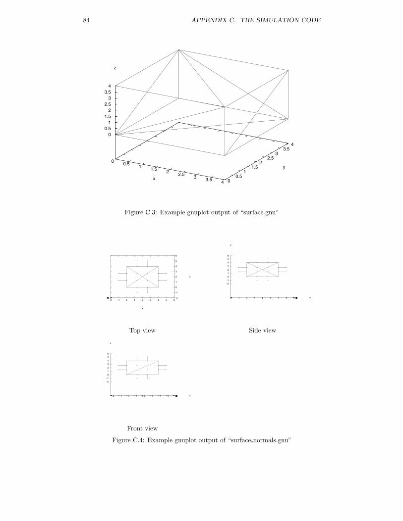
84 APPENDIX C. THE SIMULATION CODE
0 0.5 1 1.5 2 2.5 3 3.5 4x 0
0.51
1.52
2.53
3.54
y
00.5
11.5
22.5
33.5
4
z
Figure C.3: Example gnuplot output of “surface.gnu”
-2 -1 0 1 2 3 4 5 6
x
-2
-1
0
1
2
3
4
5
6
y
-2-10123456 z
Top view
-2 -1 0 1 2 3 4 5 6x -2-10123456 y
-2
-1
0
1
2
3
4
5
6
z
Side view
-2-10123456 x-2 -1 0 1 2 3 4 5 6y
-2
-1
0
1
2
3
4
5
6
z
Front view
Figure C.4: Example gnuplot output of “surface normals.gnu”
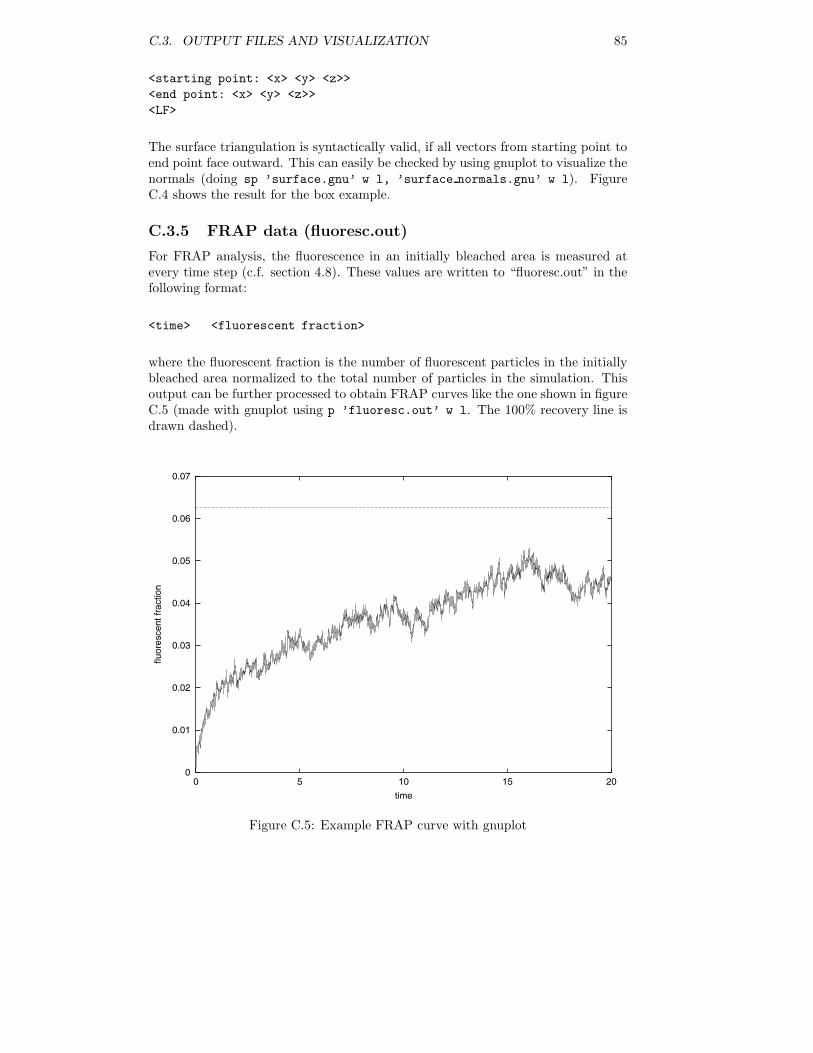
C.3. OUTPUT FILES AND VISUALIZATION 85
<starting point: <x> <y> <z>><end point: <x> <y> <z>><LF>
The surface triangulation is syntactically valid, if all vectors from starting point toend point face outward. This can easily be checked by using gnuplot to visualize thenormals (doing sp ’surface.gnu’ w l, ’surface normals.gnu’ w l). FigureC.4 shows the result for the box example.
C.3.5 FRAP data (fluoresc.out)
For FRAP analysis, the fluorescence in an initially bleached area is measured atevery time step (c.f. section 4.8). These values are written to “fluoresc.out” in thefollowing format:
<time> <fluorescent fraction>
where the fluorescent fraction is the number of fluorescent particles in the initiallybleached area normalized to the total number of particles in the simulation. Thisoutput can be further processed to obtain FRAP curves like the one shown in figureC.5 (made with gnuplot using p ’fluoresc.out’ w l. The 100% recovery line isdrawn dashed).
0
0.01
0.02
0.03
0.04
0.05
0.06
0.07
0 5 10 15 20
fluor
esce
nt fr
actio
n
time
Figure C.5: Example FRAP curve with gnuplot
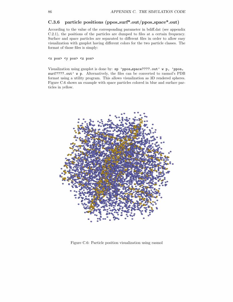
86 APPENDIX C. THE SIMULATION CODE
C.3.6 particle positions (ppos surf*.out/ppos space*.out)
According to the value of the corresponding parameter in bdiff.dat (see appendixC.2.1), the positions of the particles are dumped to files at a certain frequency.Surface and space particles are separated to different files in order to allow easyvisualization with gnuplot having different colors for the two particle classes. Theformat of those files is simply:
<x pos> <y pos> <z pos>
Visualization using gnuplot is done by: sp ’ppos space????.out’ w p, ’ppossurf????.out’ w p. Alternatively, the files can be converted to rasmol’s PDBformat using a utility program. This allows visualization as 3D rendered spheres.Figure C.6 shows an example with space particles colored in blue and surface par-ticles in yellow.
Figure C.6: Particle position visualization using rasmol
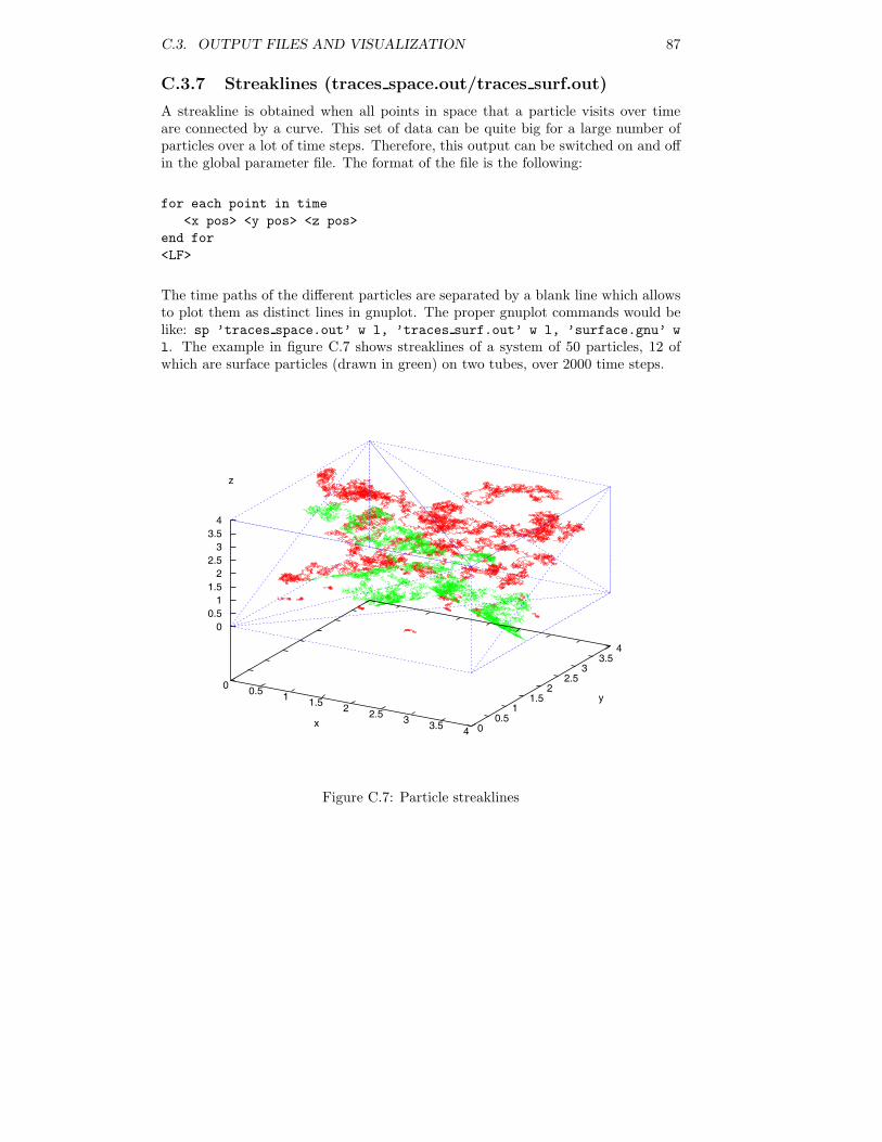
C.3. OUTPUT FILES AND VISUALIZATION 87
C.3.7 Streaklines (traces space.out/traces surf.out)
A streakline is obtained when all points in space that a particle visits over timeare connected by a curve. This set of data can be quite big for a large number ofparticles over a lot of time steps. Therefore, this output can be switched on and offin the global parameter file. The format of the file is the following:
for each point in time<x pos> <y pos> <z pos>
end for<LF>
The time paths of the different particles are separated by a blank line which allowsto plot them as distinct lines in gnuplot. The proper gnuplot commands would belike: sp ’traces space.out’ w l, ’traces surf.out’ w l, ’surface.gnu’ wl. The example in figure C.7 shows streaklines of a system of 50 particles, 12 ofwhich are surface particles (drawn in green) on two tubes, over 2000 time steps.
0 0.5 1 1.5 2 2.5 3 3.5 4x 0
0.51
1.52
2.53
3.54
y
00.5
11.5
22.5
33.5
4
z
Figure C.7: Particle streaklines
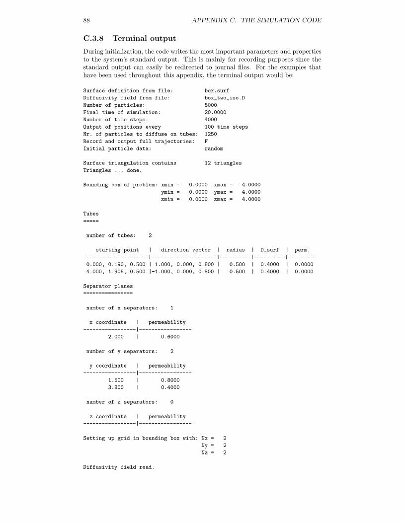
88 APPENDIX C. THE SIMULATION CODE
C.3.8 Terminal output
During initialization, the code writes the most important parameters and propertiesto the system’s standard output. This is mainly for recording purposes since thestandard output can easily be redirected to journal files. For the examples thathave been used throughout this appendix, the terminal output would be:
Surface definition from file: box.surf
Diffusivity field from file: box_two_iso.D
Number of particles: 5000
Final time of simulation: 20.0000
Number of time steps: 4000
Output of positions every 100 time steps
Nr. of particles to diffuse on tubes: 1250
Record and output full trajectories: F
Initial particle data: random
Surface triangulation contains 12 triangles
Triangles ... done.
Bounding box of problem: xmin = 0.0000 xmax = 4.0000
ymin = 0.0000 ymax = 4.0000
zmin = 0.0000 zmax = 4.0000
Tubes
=====
number of tubes: 2
starting point | direction vector | radius | D_surf | perm.
---------------------|---------------------|----------|----------|---------
0.000, 0.190, 0.500 | 1.000, 0.000, 0.800 | 0.500 | 0.4000 | 0.0000
4.000, 1.905, 0.500 |-1.000, 0.000, 0.800 | 0.500 | 0.4000 | 0.0000
Separator planes
================
number of x separators: 1
x coordinate | permeability
-----------------|-----------------
2.000 | 0.6000
number of y separators: 2
y coordinate | permeability
-----------------|-----------------
1.500 | 0.8000
3.800 | 0.4000
number of z separators: 0
z coordinate | permeability
-----------------|-----------------
Setting up grid in bounding box with: Nx = 2
Ny = 2
Nz = 2
Diffusivity field read.
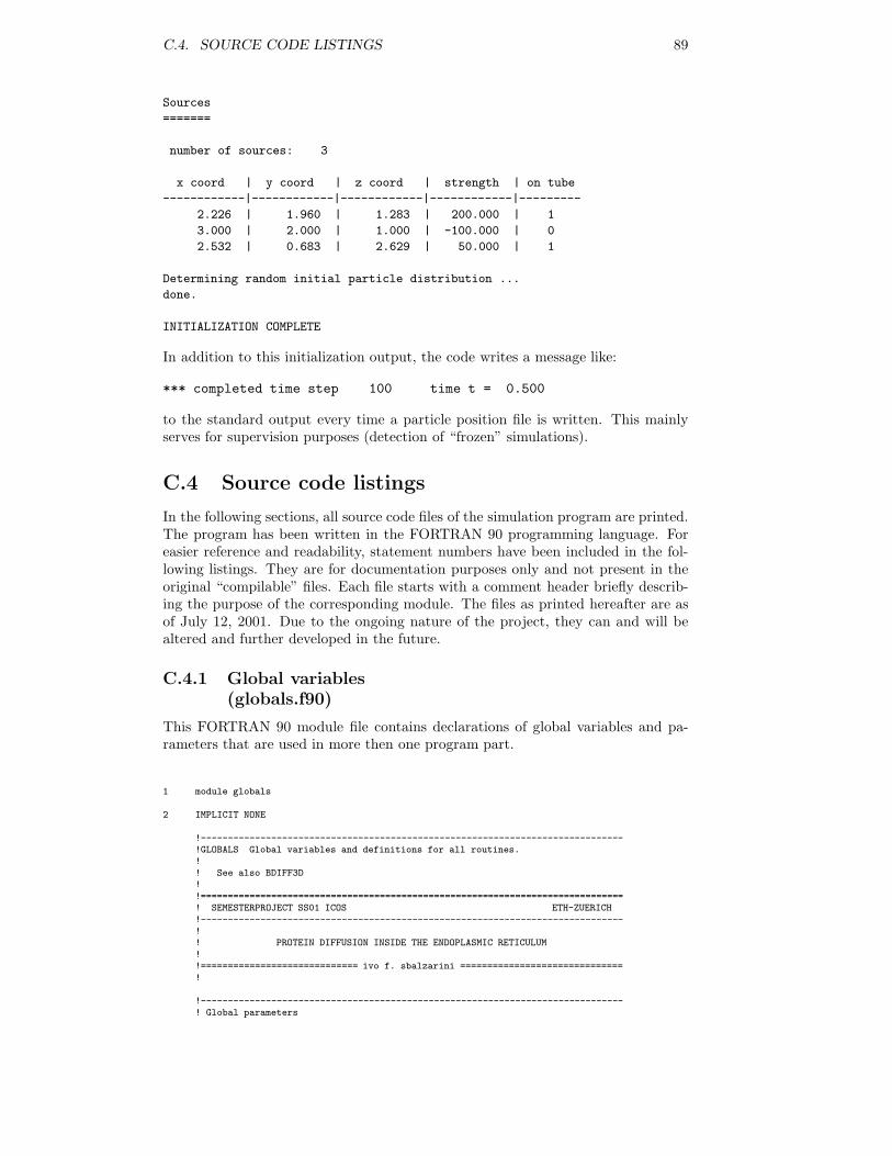
C.4. SOURCE CODE LISTINGS 89
Sources
=======
number of sources: 3
x coord | y coord | z coord | strength | on tube
------------|------------|------------|------------|---------
2.226 | 1.960 | 1.283 | 200.000 | 1
3.000 | 2.000 | 1.000 | -100.000 | 0
2.532 | 0.683 | 2.629 | 50.000 | 1
Determining random initial particle distribution ...
done.
INITIALIZATION COMPLETE
In addition to this initialization output, the code writes a message like:
*** completed time step 100 time t = 0.500
to the standard output every time a particle position file is written. This mainlyserves for supervision purposes (detection of “frozen” simulations).
C.4 Source code listings
In the following sections, all source code files of the simulation program are printed.The program has been written in the FORTRAN 90 programming language. Foreasier reference and readability, statement numbers have been included in the fol-lowing listings. They are for documentation purposes only and not present in theoriginal “compilable” files. Each file starts with a comment header briefly describ-ing the purpose of the corresponding module. The files as printed hereafter are asof July 12, 2001. Due to the ongoing nature of the project, they can and will bealtered and further developed in the future.
C.4.1 Global variables(globals.f90)
This FORTRAN 90 module file contains declarations of global variables and pa-rameters that are used in more then one program part.
1 module globals
2 IMPLICIT NONE
!------------------------------------------------------------------------------!GLOBALS Global variables and definitions for all routines.!! See also BDIFF3D!!==============================================================================! SEMESTERPROJECT SS01 ICOS ETH-ZUERICH!------------------------------------------------------------------------------!! PROTEIN DIFFUSION INSIDE THE ENDOPLASMIC RETICULUM!!============================= ivo f. sbalzarini ==============================!
!------------------------------------------------------------------------------! Global parameters
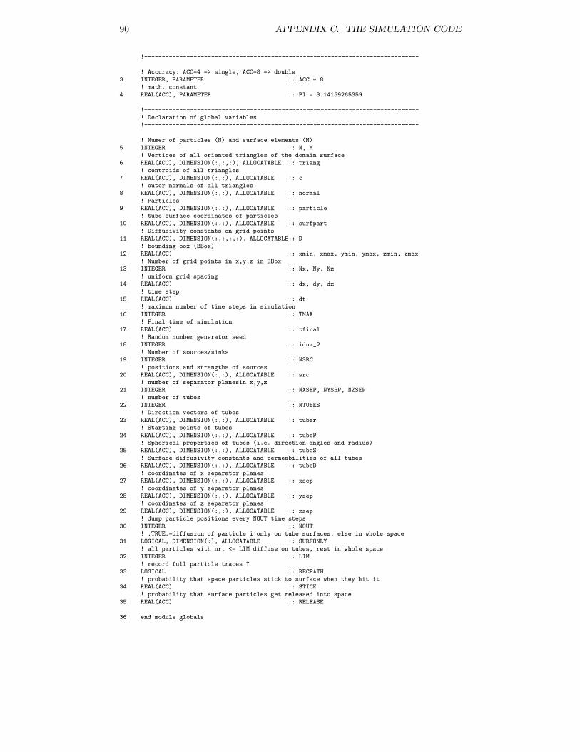
90 APPENDIX C. THE SIMULATION CODE
!------------------------------------------------------------------------------
! Accuracy: ACC=4 => single, ACC=8 => double3 INTEGER, PARAMETER :: ACC = 8
! math. constant4 REAL(ACC), PARAMETER :: PI = 3.14159265359
!------------------------------------------------------------------------------! Declaration of global variables!------------------------------------------------------------------------------
! Numer of particles (N) and surface elements (M)5 INTEGER :: N, M
! Vertices of all oriented triangles of the domain surface6 REAL(ACC), DIMENSION(:,:,:), ALLOCATABLE :: triang
! centroids of all triangles7 REAL(ACC), DIMENSION(:,:), ALLOCATABLE :: c
! outer normals of all triangles8 REAL(ACC), DIMENSION(:,:), ALLOCATABLE :: normal
! Particles9 REAL(ACC), DIMENSION(:,:), ALLOCATABLE :: particle
! tube surface coordinates of particles10 REAL(ACC), DIMENSION(:,:), ALLOCATABLE :: surfpart
! Diffusivity constants on grid points11 REAL(ACC), DIMENSION(:,:,:,:), ALLOCATABLE:: D
! bounding box (BBox)12 REAL(ACC) :: xmin, xmax, ymin, ymax, zmin, zmax
! Number of grid points in x,y,z in BBox13 INTEGER :: Nx, Ny, Nz
! uniform grid spacing14 REAL(ACC) :: dx, dy, dz
! time step15 REAL(ACC) :: dt
! maximum number of time steps in simulation16 INTEGER :: TMAX
! Final time of simulation17 REAL(ACC) :: tfinal
! Random number generator seed18 INTEGER :: idum_2
! Number of sources/sinks19 INTEGER :: NSRC
! positions and strengths of sources20 REAL(ACC), DIMENSION(:,:), ALLOCATABLE :: src
! number of separator planesin x,y,z21 INTEGER :: NXSEP, NYSEP, NZSEP
! number of tubes22 INTEGER :: NTUBES
! Direction vectors of tubes23 REAL(ACC), DIMENSION(:,:), ALLOCATABLE :: tuber
! Starting points of tubes24 REAL(ACC), DIMENSION(:,:), ALLOCATABLE :: tubeP
! Spherical properties of tubes (i.e. direction angles and radius)25 REAL(ACC), DIMENSION(:,:), ALLOCATABLE :: tubeS
! Surface diffusivity constants and permeabilities of all tubes26 REAL(ACC), DIMENSION(:,:), ALLOCATABLE :: tubeD
! coordinates of x separator planes27 REAL(ACC), DIMENSION(:,:), ALLOCATABLE :: xsep
! coordinates of y separator planes28 REAL(ACC), DIMENSION(:,:), ALLOCATABLE :: ysep
! coordinates of z separator planes29 REAL(ACC), DIMENSION(:,:), ALLOCATABLE :: zsep
! dump particle positions every NOUT time steps30 INTEGER :: NOUT
! .TRUE.=diffusion of particle i only on tube surfaces, else in whole space31 LOGICAL, DIMENSION(:), ALLOCATABLE :: SURFONLY
! all particles with nr. <= LIM diffuse on tubes, rest in whole space32 INTEGER :: LIM
! record full particle traces ?33 LOGICAL :: RECPATH
! probability that space particles stick to surface when they hit it34 REAL(ACC) :: STICK
! probability that surface particles get released into space35 REAL(ACC) :: RELEASE
36 end module globals
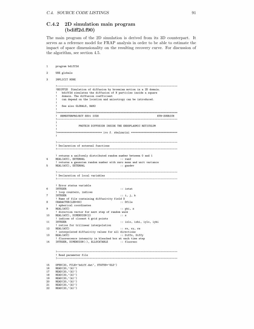
C.4. SOURCE CODE LISTINGS 91
C.4.2 2D simulation main program(bdiff2d.f90)
The main program of the 2D simulation is derived from its 3D counterpart. Itserves as a reference model for FRAP analysis in order to be able to estimate theimpact of space dimensionality on the resulting recovery curve. For discussion ofthe algorithm, see section 4.5.
1 program bdiff2d
2 USE globals
3 IMPLICIT NONE
!------------------------------------------------------------------------------!BDIFF2D Simulation of diffusion by brownian motion in a 2D domain.! bdiff2d simulates the diffusion of N particles inside a square! domain. The diffusion coefficient! can depend on the location and anisotropy can be introduced.!! See also GLOBALS, RAN2!!==============================================================================! SEMESTERPROJECT SS01 ICOS ETH-ZUERICH!------------------------------------------------------------------------------!! PROTEIN DIFFUSION INSIDE THE ENDOPLASMIC RETICULUM!!============================= ivo f. sbalzarini ==============================!
!------------------------------------------------------------------------------! Declaration of external functions!------------------------------------------------------------------------------
! returns a uniformly distributed random number between 0 and 14 REAL(ACC), EXTERNAL :: ran2
! returns a gaussian random number with zero mean and unit variance5 REAL(ACC), EXTERNAL :: gasdev
!------------------------------------------------------------------------------! Declaration of local variables!------------------------------------------------------------------------------
! Error status variable6 INTEGER :: istat
! loop counters, indices7 INTEGER :: i, j, k
! Name of file containing diffusivity field D8 CHARACTER(LEN=80) :: Dfile
! spherical coordinates9 REAL(ACC) :: phi, z
! direction vector for next step of random walk10 REAL(ACC), DIMENSION(2) :: s
! indices of closest 4 grid points11 INTEGER :: ixlo, ixhi, iylo, iyhi
! ratios for trilinear interpolation12 REAL(ACC) :: rx, ry, rz
! interpolated diffusivity values for all directions13 REAL(ACC) :: Diffx, Diffy
! fluorescence intensity in bleached box at each time step14 INTEGER, DIMENSION(:), ALLOCATABLE :: fluoresc
!------------------------------------------------------------------------------! Read parameter file!------------------------------------------------------------------------------
15 OPEN(20, FILE=’bdiff.dat’, STATUS=’OLD’)16 READ(20,’(A)’)17 READ(20,’(A)’)18 READ(20,’(A)’)19 READ(20,’(A)’)20 READ(20,’(A)’)21 READ(20,’(A)’)22 READ(20,’(A)’)
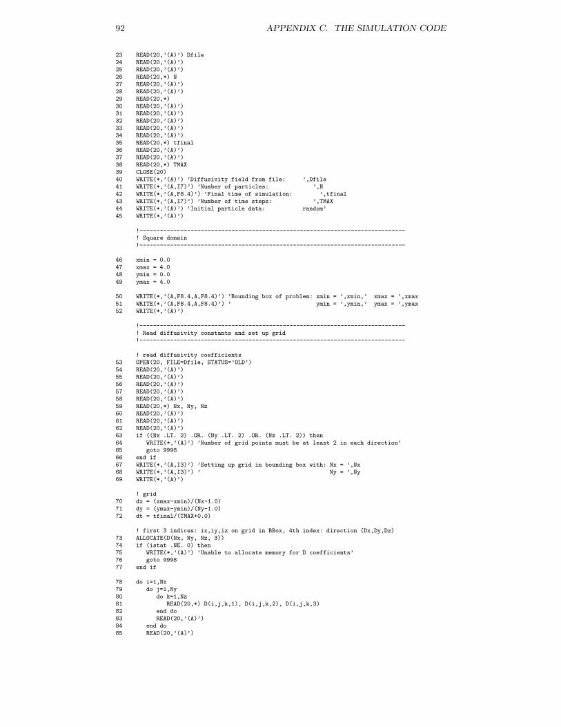
92 APPENDIX C. THE SIMULATION CODE
23 READ(20,’(A)’) Dfile24 READ(20,’(A)’)25 READ(20,’(A)’)26 READ(20,*) N27 READ(20,’(A)’)28 READ(20,’(A)’)29 READ(20,*)30 READ(20,’(A)’)31 READ(20,’(A)’)32 READ(20,’(A)’)33 READ(20,’(A)’)34 READ(20,’(A)’)35 READ(20,*) tfinal36 READ(20,’(A)’)37 READ(20,’(A)’)38 READ(20,*) TMAX39 CLOSE(20)40 WRITE(*,’(A)’) ’Diffusivity field from file: ’,Dfile41 WRITE(*,’(A,I7)’) ’Number of particles: ’,N42 WRITE(*,’(A,F8.4)’) ’Final time of simulation: ’,tfinal43 WRITE(*,’(A,I7)’) ’Number of time steps: ’,TMAX44 WRITE(*,’(A)’) ’Initial particle data: random’45 WRITE(*,’(A)’)
!------------------------------------------------------------------------------! Square domain!------------------------------------------------------------------------------
46 xmin = 0.047 xmax = 4.048 ymin = 0.049 ymax = 4.0
50 WRITE(*,’(A,F8.4,A,F8.4)’) ’Bounding box of problem: xmin = ’,xmin,’ xmax = ’,xmax51 WRITE(*,’(A,F8.4,A,F8.4)’) ’ ymin = ’,ymin,’ ymax = ’,ymax52 WRITE(*,’(A)’)
!------------------------------------------------------------------------------! Read diffusivity constants and set up grid!------------------------------------------------------------------------------
! read diffusivity coefficients53 OPEN(20, FILE=Dfile, STATUS=’OLD’)54 READ(20,’(A)’)55 READ(20,’(A)’)56 READ(20,’(A)’)57 READ(20,’(A)’)58 READ(20,’(A)’)59 READ(20,*) Nx, Ny, Nz60 READ(20,’(A)’)61 READ(20,’(A)’)62 READ(20,’(A)’)63 if ((Nx .LT. 2) .OR. (Ny .LT. 2) .OR. (Nz .LT. 2)) then64 WRITE(*,’(A)’) ’Number of grid points must be at least 2 in each direction’65 goto 999866 end if67 WRITE(*,’(A,I3)’) ’Setting up grid in bounding box with: Nx = ’,Nx68 WRITE(*,’(A,I3)’) ’ Ny = ’,Ny69 WRITE(*,’(A)’)
! grid70 dx = (xmax-xmin)/(Nx-1.0)71 dy = (ymax-ymin)/(Ny-1.0)72 dt = tfinal/(TMAX+0.0)
! first 3 indices: ix,iy,iz on grid in BBox, 4th index: direction (Dx,Dy,Dz)73 ALLOCATE(D(Nx, Ny, Nz, 3))74 if (istat .NE. 0) then75 WRITE(*,’(A)’) ’Unable to allocate memory for D coefficients’76 goto 999877 end if
78 do i=1,Nx79 do j=1,Ny80 do k=1,Nz81 READ(20,*) D(i,j,k,1), D(i,j,k,2), D(i,j,k,3)82 end do83 READ(20,’(A)’)84 end do85 READ(20,’(A)’)
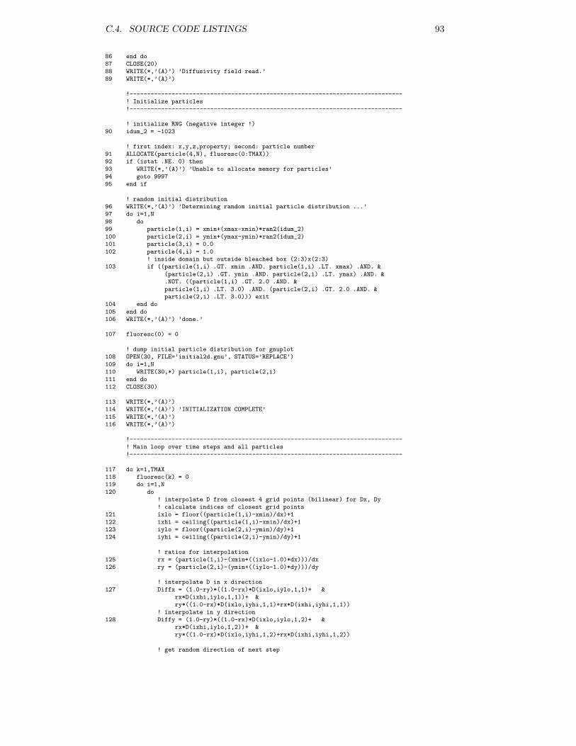
C.4. SOURCE CODE LISTINGS 93
86 end do87 CLOSE(20)88 WRITE(*,’(A)’) ’Diffusivity field read.’89 WRITE(*,’(A)’)
!------------------------------------------------------------------------------! Initialize particles!------------------------------------------------------------------------------
! initialize RNG (negative integer !)90 idum_2 = -1023
! first index: x,y,z,property; second: particle number91 ALLOCATE(particle(4,N), fluoresc(0:TMAX))92 if (istat .NE. 0) then93 WRITE(*,’(A)’) ’Unable to allocate memory for particles’94 goto 999795 end if
! random initial distribution96 WRITE(*,’(A)’) ’Determining random initial particle distribution ...’97 do i=1,N98 do99 particle(1,i) = xmin+(xmax-xmin)*ran2(idum_2)100 particle(2,i) = ymin+(ymax-ymin)*ran2(idum_2)101 particle(3,i) = 0.0102 particle(4,i) = 1.0
! inside domain but outside bleached box (2:3)x(2:3)103 if ((particle(1,i) .GT. xmin .AND. particle(1,i) .LT. xmax) .AND. &
(particle(2,i) .GT. ymin .AND. particle(2,i) .LT. ymax) .AND. &.NOT. ((particle(1,i) .GT. 2.0 .AND. &particle(1,i) .LT. 3.0) .AND. (particle(2,i) .GT. 2.0 .AND. &particle(2,i) .LT. 3.0))) exit
104 end do105 end do106 WRITE(*,’(A)’) ’done.’
107 fluoresc(0) = 0
! dump initial particle distribution for gnuplot108 OPEN(30, FILE=’initial2d.gnu’, STATUS=’REPLACE’)109 do i=1,N110 WRITE(30,*) particle(1,i), particle(2,i)111 end do112 CLOSE(30)
113 WRITE(*,’(A)’)114 WRITE(*,’(A)’) ’INITIALIZATION COMPLETE’115 WRITE(*,’(A)’)116 WRITE(*,’(A)’)
!------------------------------------------------------------------------------! Main loop over time steps and all particles!------------------------------------------------------------------------------
117 do k=1,TMAX118 fluoresc(k) = 0119 do i=1,N120 do
! interpolate D from closest 4 grid points (bilinear) for Dx, Dy! calculate indices of closest grid points
121 ixlo = floor((particle(1,i)-xmin)/dx)+1122 ixhi = ceiling((particle(1,i)-xmin)/dx)+1123 iylo = floor((particle(2,i)-ymin)/dy)+1124 iyhi = ceiling((particle(2,i)-ymin)/dy)+1
! ratios for interpolation125 rx = (particle(1,i)-(xmin+((ixlo-1.0)*dx)))/dx126 ry = (particle(2,i)-(ymin+((iylo-1.0)*dy)))/dy
! interpolate D in x direction127 Diffx = (1.0-ry)*((1.0-rx)*D(ixlo,iylo,1,1)+ &
rx*D(ixhi,iylo,1,1))+ &ry*((1.0-rx)*D(ixlo,iyhi,1,1)+rx*D(ixhi,iyhi,1,1))
! interpolate in y direction128 Diffy = (1.0-ry)*((1.0-rx)*D(ixlo,iylo,1,2)+ &
rx*D(ixhi,iylo,1,2))+ &ry*((1.0-rx)*D(ixlo,iyhi,1,2)+rx*D(ixhi,iyhi,1,2))
! get random direction of next step
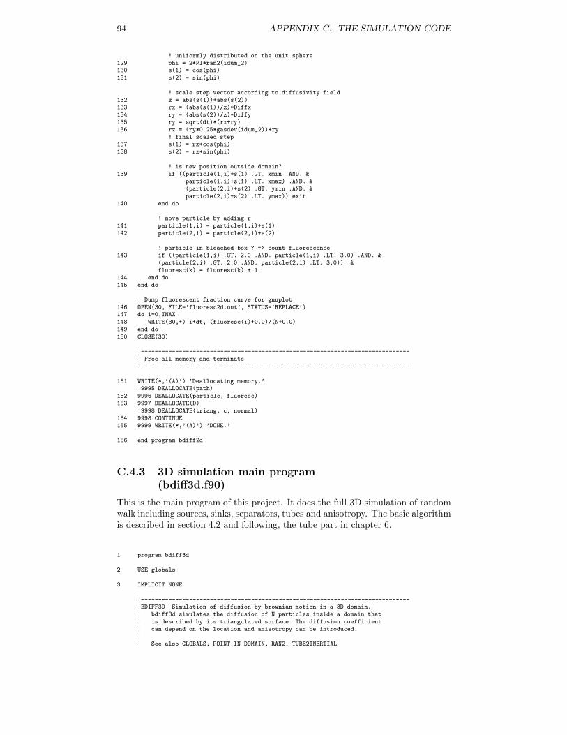
94 APPENDIX C. THE SIMULATION CODE
! uniformly distributed on the unit sphere129 phi = 2*PI*ran2(idum_2)130 s(1) = cos(phi)131 s(2) = sin(phi)
! scale step vector according to diffusivity field132 z = abs(s(1))+abs(s(2))133 rx = (abs(s(1))/z)*Diffx134 ry = (abs(s(2))/z)*Diffy135 ry = sqrt(dt)*(rx+ry)136 rz = (ry*0.25*gasdev(idum_2))+ry
! final scaled step137 s(1) = rz*cos(phi)138 s(2) = rz*sin(phi)
! is new position outside domain?139 if ((particle(1,i)+s(1) .GT. xmin .AND. &
particle(1,i)+s(1) .LT. xmax) .AND. &(particle(2,i)+s(2) .GT. ymin .AND. &particle(2,i)+s(2) .LT. ymax)) exit
140 end do
! move particle by adding r141 particle(1,i) = particle(1,i)+s(1)142 particle(2,i) = particle(2,i)+s(2)
! particle in bleached box ? => count fluorescence143 if ((particle(1,i) .GT. 2.0 .AND. particle(1,i) .LT. 3.0) .AND. &
(particle(2,i) .GT. 2.0 .AND. particle(2,i) .LT. 3.0)) &fluoresc(k) = fluoresc(k) + 1
144 end do145 end do
! Dump fluorescent fraction curve for gnuplot146 OPEN(30, FILE=’fluoresc2d.out’, STATUS=’REPLACE’)147 do i=0,TMAX148 WRITE(30,*) i*dt, (fluoresc(i)+0.0)/(N+0.0)149 end do150 CLOSE(30)
!------------------------------------------------------------------------------! Free all memory and terminate!------------------------------------------------------------------------------
151 WRITE(*,’(A)’) ’Deallocating memory.’!9995 DEALLOCATE(path)
152 9996 DEALLOCATE(particle, fluoresc)153 9997 DEALLOCATE(D)
!9998 DEALLOCATE(triang, c, normal)154 9998 CONTINUE155 9999 WRITE(*,’(A)’) ’DONE.’
156 end program bdiff2d
C.4.3 3D simulation main program(bdiff3d.f90)
This is the main program of this project. It does the full 3D simulation of randomwalk including sources, sinks, separators, tubes and anisotropy. The basic algorithmis described in section 4.2 and following, the tube part in chapter 6.
1 program bdiff3d
2 USE globals
3 IMPLICIT NONE
!------------------------------------------------------------------------------!BDIFF3D Simulation of diffusion by brownian motion in a 3D domain.! bdiff3d simulates the diffusion of N particles inside a domain that! is described by its triangulated surface. The diffusion coefficient! can depend on the location and anisotropy can be introduced.!! See also GLOBALS, POINT_IN_DOMAIN, RAN2, TUBE2INERTIAL
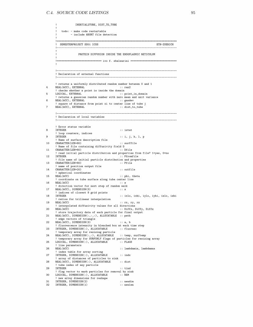
C.4. SOURCE CODE LISTINGS 95
! INERTIAL2TUBE, DIST_TO_TUBE!! todo: - make code restartable! - include ABORT file detection!!==============================================================================! SEMESTERPROJECT SS01 ICOS ETH-ZUERICH!------------------------------------------------------------------------------!! PROTEIN DIFFUSION INSIDE THE ENDOPLASMIC RETICULUM!!============================= ivo f. sbalzarini ==============================!
!------------------------------------------------------------------------------! Declaration of external functions!------------------------------------------------------------------------------
! returns a uniformly distributed random number between 0 and 14 REAL(ACC), EXTERNAL :: ran2
! checks whether a point is inside the domain5 LOGICAL, EXTERNAL :: point_in_domain
! returns a gaussian random number with zero mean and unit variance6 REAL(ACC), EXTERNAL :: gasdev
! square of distance from point xi to center line of tube j7 REAL(ACC), EXTERNAL :: dist_to_tube
!------------------------------------------------------------------------------! Declaration of local variables!------------------------------------------------------------------------------
! Error status variable8 INTEGER :: istat
! loop counters, indices9 INTEGER :: i, j, k, l, p
! Name of surface description file10 CHARACTER(LEN=80) :: surffile
! Name of file containing diffusivity field D11 CHARACTER(LEN=80) :: Dfile
! read initial particle distribution and properties from file? 1=yes, 0=no12 INTEGER :: Pfromfile
! file name of initial particle distribution and properties13 CHARACTER(LEN=80) :: Pfile
! name of position output file14 CHARACTER(LEN=20) :: outfile
! spherical coordinates15 REAL(ACC) :: phi, theta
! coordinate on tube surface along tube center line16 REAL(ACC) :: z
! direction vector for next step of random walk17 REAL(ACC), DIMENSION(3) :: s
! indices of closest 8 grid points18 INTEGER :: ixlo, ixhi, iylo, iyhi, izlo, izhi
! ratios for trilinear interpolation19 REAL(ACC) :: rx, ry, rz
! interpolated diffusivity values for all directions20 REAL(ACC) :: Diffx, Diffy, Diffz
! store trajectory data of each particle for final output21 REAL(ACC), DIMENSION(:,:,:), ALLOCATABLE :: path
! edge vectors of triangle22 REAL(ACC), DIMENSION(3) :: a, b
! fluorescence intensity in bleached box at each time step23 INTEGER, DIMENSION(:), ALLOCATABLE :: fluoresc
! temporary array for resizing particle24 REAL(ACC), DIMENSION(:,:), ALLOCATABLE :: temp, surftemp
! temporary array for SURFONLY flags of particles for resizing array25 LOGICAL, DIMENSION(:), ALLOCATABLE :: FLAGS
! line parameters26 REAL(ACC) :: lambdamin, lambdamax
! index table for array sorting27 INTEGER, DIMENSION(:), ALLOCATABLE :: indx
! array of distances of particles to sink28 REAL(ACC), DIMENSION(:), ALLOCATABLE :: dist
! tube index of any particle29 INTEGER :: tind
! flag vector to mark particles for removal by sink30 LOGICAL, DIMENSION(:), ALLOCATABLE :: REM
! new array dimensions for reshape31 INTEGER, DIMENSION(2) :: newdim32 INTEGER, DIMENSION(1) :: newlen
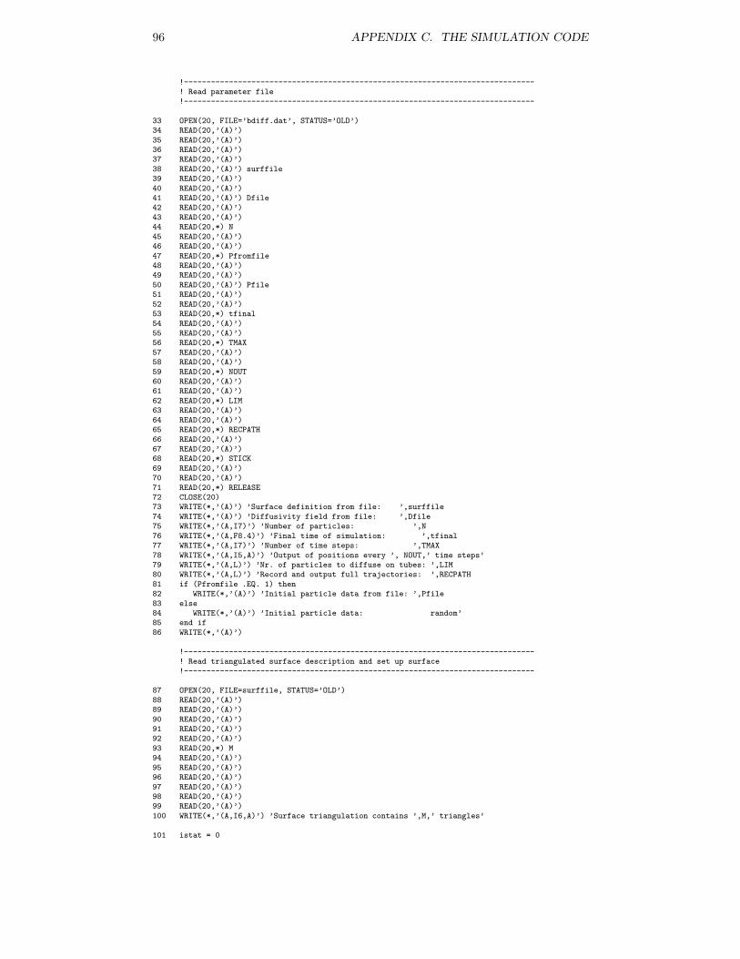
96 APPENDIX C. THE SIMULATION CODE
!------------------------------------------------------------------------------! Read parameter file!------------------------------------------------------------------------------
33 OPEN(20, FILE=’bdiff.dat’, STATUS=’OLD’)34 READ(20,’(A)’)35 READ(20,’(A)’)36 READ(20,’(A)’)37 READ(20,’(A)’)38 READ(20,’(A)’) surffile39 READ(20,’(A)’)40 READ(20,’(A)’)41 READ(20,’(A)’) Dfile42 READ(20,’(A)’)43 READ(20,’(A)’)44 READ(20,*) N45 READ(20,’(A)’)46 READ(20,’(A)’)47 READ(20,*) Pfromfile48 READ(20,’(A)’)49 READ(20,’(A)’)50 READ(20,’(A)’) Pfile51 READ(20,’(A)’)52 READ(20,’(A)’)53 READ(20,*) tfinal54 READ(20,’(A)’)55 READ(20,’(A)’)56 READ(20,*) TMAX57 READ(20,’(A)’)58 READ(20,’(A)’)59 READ(20,*) NOUT60 READ(20,’(A)’)61 READ(20,’(A)’)62 READ(20,*) LIM63 READ(20,’(A)’)64 READ(20,’(A)’)65 READ(20,*) RECPATH66 READ(20,’(A)’)67 READ(20,’(A)’)68 READ(20,*) STICK69 READ(20,’(A)’)70 READ(20,’(A)’)71 READ(20,*) RELEASE72 CLOSE(20)73 WRITE(*,’(A)’) ’Surface definition from file: ’,surffile74 WRITE(*,’(A)’) ’Diffusivity field from file: ’,Dfile75 WRITE(*,’(A,I7)’) ’Number of particles: ’,N76 WRITE(*,’(A,F8.4)’) ’Final time of simulation: ’,tfinal77 WRITE(*,’(A,I7)’) ’Number of time steps: ’,TMAX78 WRITE(*,’(A,I5,A)’) ’Output of positions every ’, NOUT,’ time steps’79 WRITE(*,’(A,L)’) ’Nr. of particles to diffuse on tubes: ’,LIM80 WRITE(*,’(A,L)’) ’Record and output full trajectories: ’,RECPATH81 if (Pfromfile .EQ. 1) then82 WRITE(*,’(A)’) ’Initial particle data from file: ’,Pfile83 else84 WRITE(*,’(A)’) ’Initial particle data: random’85 end if86 WRITE(*,’(A)’)
!------------------------------------------------------------------------------! Read triangulated surface description and set up surface!------------------------------------------------------------------------------
87 OPEN(20, FILE=surffile, STATUS=’OLD’)88 READ(20,’(A)’)89 READ(20,’(A)’)90 READ(20,’(A)’)91 READ(20,’(A)’)92 READ(20,’(A)’)93 READ(20,*) M94 READ(20,’(A)’)95 READ(20,’(A)’)96 READ(20,’(A)’)97 READ(20,’(A)’)98 READ(20,’(A)’)99 READ(20,’(A)’)100 WRITE(*,’(A,I6,A)’) ’Surface triangulation contains ’,M,’ triangles’
101 istat = 0
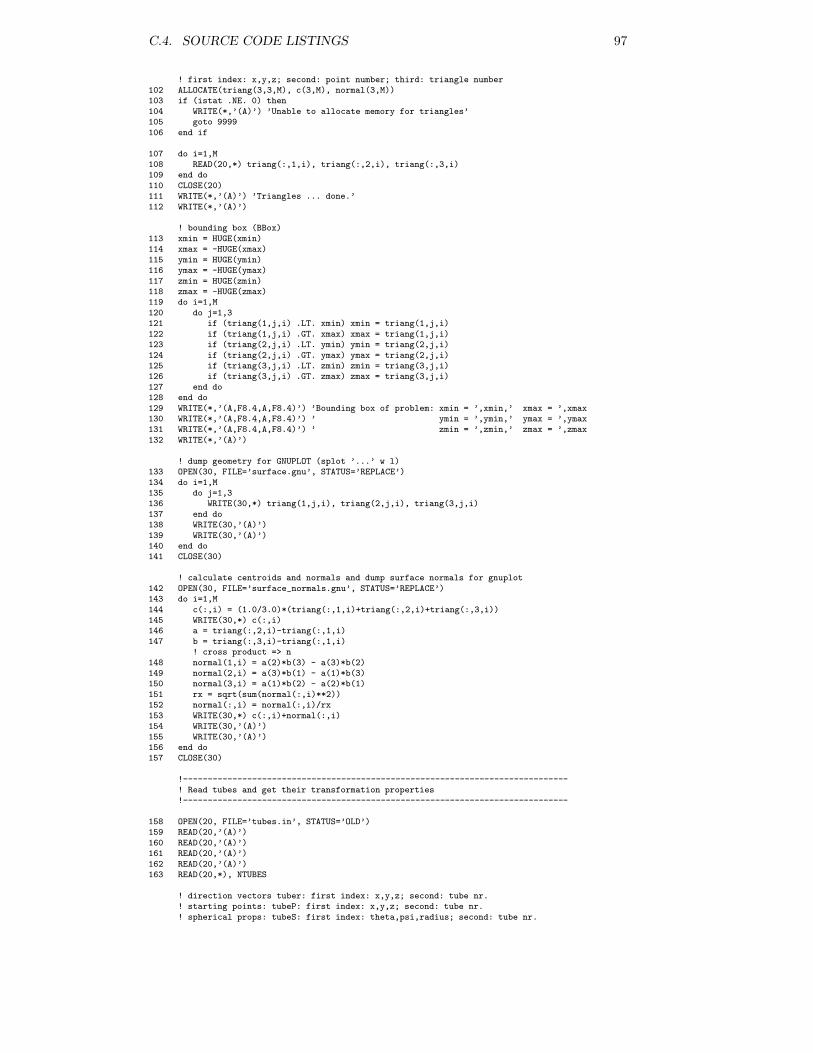
C.4. SOURCE CODE LISTINGS 97
! first index: x,y,z; second: point number; third: triangle number102 ALLOCATE(triang(3,3,M), c(3,M), normal(3,M))103 if (istat .NE. 0) then104 WRITE(*,’(A)’) ’Unable to allocate memory for triangles’105 goto 9999106 end if
107 do i=1,M108 READ(20,*) triang(:,1,i), triang(:,2,i), triang(:,3,i)109 end do110 CLOSE(20)111 WRITE(*,’(A)’) ’Triangles ... done.’112 WRITE(*,’(A)’)
! bounding box (BBox)113 xmin = HUGE(xmin)114 xmax = -HUGE(xmax)115 ymin = HUGE(ymin)116 ymax = -HUGE(ymax)117 zmin = HUGE(zmin)118 zmax = -HUGE(zmax)119 do i=1,M120 do j=1,3121 if (triang(1,j,i) .LT. xmin) xmin = triang(1,j,i)122 if (triang(1,j,i) .GT. xmax) xmax = triang(1,j,i)123 if (triang(2,j,i) .LT. ymin) ymin = triang(2,j,i)124 if (triang(2,j,i) .GT. ymax) ymax = triang(2,j,i)125 if (triang(3,j,i) .LT. zmin) zmin = triang(3,j,i)126 if (triang(3,j,i) .GT. zmax) zmax = triang(3,j,i)127 end do128 end do129 WRITE(*,’(A,F8.4,A,F8.4)’) ’Bounding box of problem: xmin = ’,xmin,’ xmax = ’,xmax130 WRITE(*,’(A,F8.4,A,F8.4)’) ’ ymin = ’,ymin,’ ymax = ’,ymax131 WRITE(*,’(A,F8.4,A,F8.4)’) ’ zmin = ’,zmin,’ zmax = ’,zmax132 WRITE(*,’(A)’)
! dump geometry for GNUPLOT (splot ’...’ w l)133 OPEN(30, FILE=’surface.gnu’, STATUS=’REPLACE’)134 do i=1,M135 do j=1,3136 WRITE(30,*) triang(1,j,i), triang(2,j,i), triang(3,j,i)137 end do138 WRITE(30,’(A)’)139 WRITE(30,’(A)’)140 end do141 CLOSE(30)
! calculate centroids and normals and dump surface normals for gnuplot142 OPEN(30, FILE=’surface_normals.gnu’, STATUS=’REPLACE’)143 do i=1,M144 c(:,i) = (1.0/3.0)*(triang(:,1,i)+triang(:,2,i)+triang(:,3,i))145 WRITE(30,*) c(:,i)146 a = triang(:,2,i)-triang(:,1,i)147 b = triang(:,3,i)-triang(:,1,i)
! cross product => n148 normal(1,i) = a(2)*b(3) - a(3)*b(2)149 normal(2,i) = a(3)*b(1) - a(1)*b(3)150 normal(3,i) = a(1)*b(2) - a(2)*b(1)151 rx = sqrt(sum(normal(:,i)**2))152 normal(:,i) = normal(:,i)/rx153 WRITE(30,*) c(:,i)+normal(:,i)154 WRITE(30,’(A)’)155 WRITE(30,’(A)’)156 end do157 CLOSE(30)
!------------------------------------------------------------------------------! Read tubes and get their transformation properties!------------------------------------------------------------------------------
158 OPEN(20, FILE=’tubes.in’, STATUS=’OLD’)159 READ(20,’(A)’)160 READ(20,’(A)’)161 READ(20,’(A)’)162 READ(20,’(A)’)163 READ(20,*), NTUBES
! direction vectors tuber: first index: x,y,z; second: tube nr.! starting points: tubeP: first index: x,y,z; second: tube nr.! spherical props: tubeS: first index: theta,psi,radius; second: tube nr.
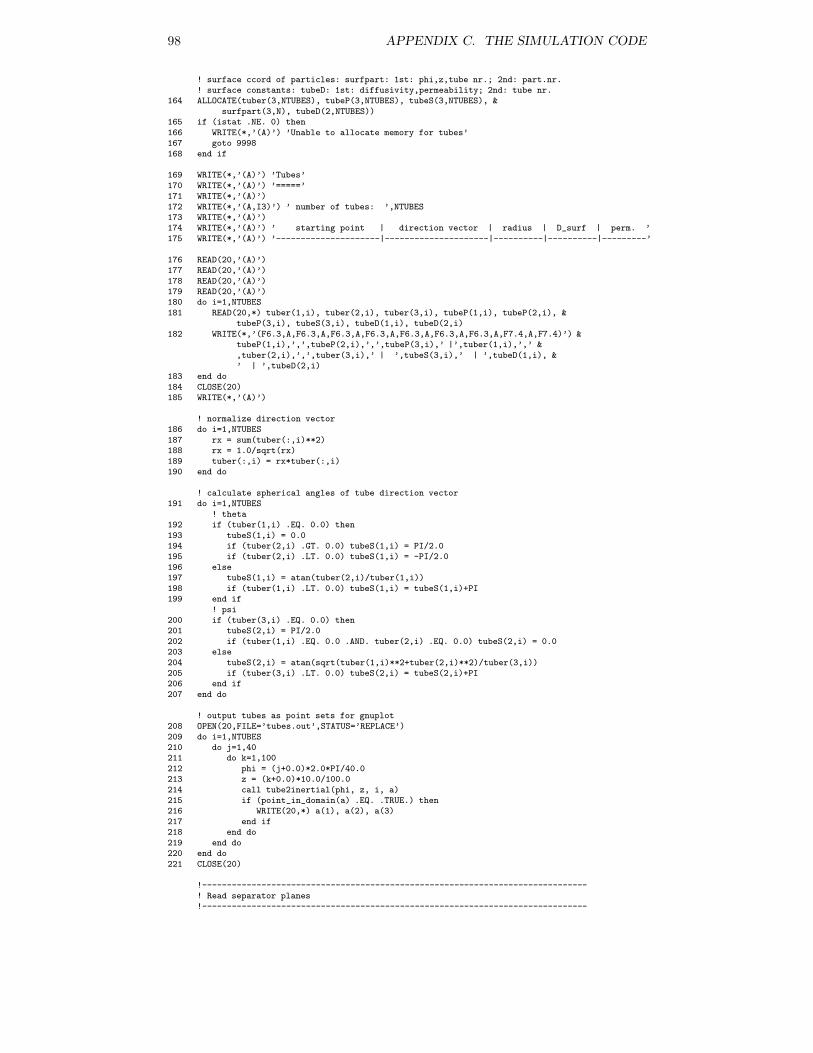
98 APPENDIX C. THE SIMULATION CODE
! surface ccord of particles: surfpart: 1st: phi,z,tube nr.; 2nd: part.nr.! surface constants: tubeD: 1st: diffusivity,permeability; 2nd: tube nr.
164 ALLOCATE(tuber(3,NTUBES), tubeP(3,NTUBES), tubeS(3,NTUBES), &surfpart(3,N), tubeD(2,NTUBES))
165 if (istat .NE. 0) then166 WRITE(*,’(A)’) ’Unable to allocate memory for tubes’167 goto 9998168 end if
169 WRITE(*,’(A)’) ’Tubes’170 WRITE(*,’(A)’) ’=====’171 WRITE(*,’(A)’)172 WRITE(*,’(A,I3)’) ’ number of tubes: ’,NTUBES173 WRITE(*,’(A)’)174 WRITE(*,’(A)’) ’ starting point | direction vector | radius | D_surf | perm. ’175 WRITE(*,’(A)’) ’---------------------|---------------------|----------|----------|---------’
176 READ(20,’(A)’)177 READ(20,’(A)’)178 READ(20,’(A)’)179 READ(20,’(A)’)180 do i=1,NTUBES181 READ(20,*) tuber(1,i), tuber(2,i), tuber(3,i), tubeP(1,i), tubeP(2,i), &
tubeP(3,i), tubeS(3,i), tubeD(1,i), tubeD(2,i)182 WRITE(*,’(F6.3,A,F6.3,A,F6.3,A,F6.3,A,F6.3,A,F6.3,A,F6.3,A,F7.4,A,F7.4)’) &
tubeP(1,i),’,’,tubeP(2,i),’,’,tubeP(3,i),’ |’,tuber(1,i),’,’ &,tuber(2,i),’,’,tuber(3,i),’ | ’,tubeS(3,i),’ | ’,tubeD(1,i), &’ | ’,tubeD(2,i)
183 end do184 CLOSE(20)185 WRITE(*,’(A)’)
! normalize direction vector186 do i=1,NTUBES187 rx = sum(tuber(:,i)**2)188 rx = 1.0/sqrt(rx)189 tuber(:,i) = rx*tuber(:,i)190 end do
! calculate spherical angles of tube direction vector191 do i=1,NTUBES
! theta192 if (tuber(1,i) .EQ. 0.0) then193 tubeS(1,i) = 0.0194 if (tuber(2,i) .GT. 0.0) tubeS(1,i) = PI/2.0195 if (tuber(2,i) .LT. 0.0) tubeS(1,i) = -PI/2.0196 else197 tubeS(1,i) = atan(tuber(2,i)/tuber(1,i))198 if (tuber(1,i) .LT. 0.0) tubeS(1,i) = tubeS(1,i)+PI199 end if
! psi200 if (tuber(3,i) .EQ. 0.0) then201 tubeS(2,i) = PI/2.0202 if (tuber(1,i) .EQ. 0.0 .AND. tuber(2,i) .EQ. 0.0) tubeS(2,i) = 0.0203 else204 tubeS(2,i) = atan(sqrt(tuber(1,i)**2+tuber(2,i)**2)/tuber(3,i))205 if (tuber(3,i) .LT. 0.0) tubeS(2,i) = tubeS(2,i)+PI206 end if207 end do
! output tubes as point sets for gnuplot208 OPEN(20,FILE=’tubes.out’,STATUS=’REPLACE’)209 do i=1,NTUBES210 do j=1,40211 do k=1,100212 phi = (j+0.0)*2.0*PI/40.0213 z = (k+0.0)*10.0/100.0214 call tube2inertial(phi, z, i, a)215 if (point_in_domain(a) .EQ. .TRUE.) then216 WRITE(20,*) a(1), a(2), a(3)217 end if218 end do219 end do220 end do221 CLOSE(20)
!------------------------------------------------------------------------------! Read separator planes!------------------------------------------------------------------------------
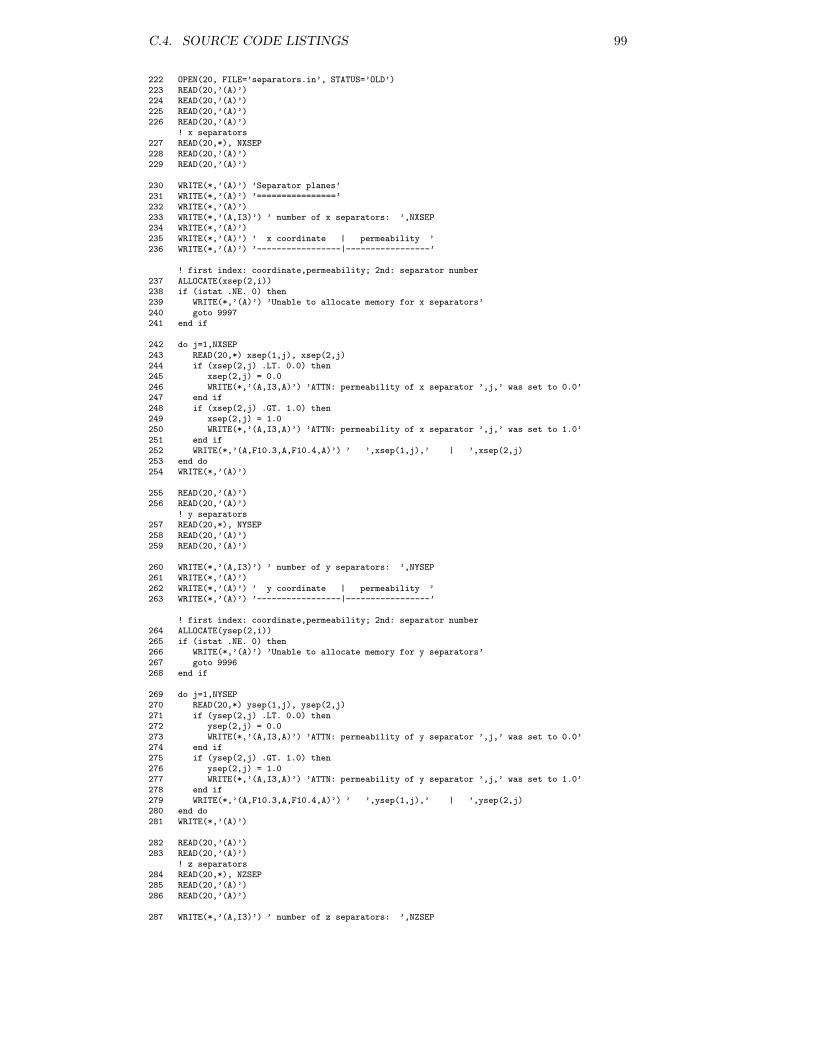
C.4. SOURCE CODE LISTINGS 99
222 OPEN(20, FILE=’separators.in’, STATUS=’OLD’)223 READ(20,’(A)’)224 READ(20,’(A)’)225 READ(20,’(A)’)226 READ(20,’(A)’)
! x separators227 READ(20,*), NXSEP228 READ(20,’(A)’)229 READ(20,’(A)’)
230 WRITE(*,’(A)’) ’Separator planes’231 WRITE(*,’(A)’) ’================’232 WRITE(*,’(A)’)233 WRITE(*,’(A,I3)’) ’ number of x separators: ’,NXSEP234 WRITE(*,’(A)’)235 WRITE(*,’(A)’) ’ x coordinate | permeability ’236 WRITE(*,’(A)’) ’-----------------|-----------------’
! first index: coordinate,permeability; 2nd: separator number237 ALLOCATE(xsep(2,i))238 if (istat .NE. 0) then239 WRITE(*,’(A)’) ’Unable to allocate memory for x separators’240 goto 9997241 end if
242 do j=1,NXSEP243 READ(20,*) xsep(1,j), xsep(2,j)244 if (xsep(2,j) .LT. 0.0) then245 xsep(2,j) = 0.0246 WRITE(*,’(A,I3,A)’) ’ATTN: permeability of x separator ’,j,’ was set to 0.0’247 end if248 if (xsep(2,j) .GT. 1.0) then249 xsep(2,j) = 1.0250 WRITE(*,’(A,I3,A)’) ’ATTN: permeability of x separator ’,j,’ was set to 1.0’251 end if252 WRITE(*,’(A,F10.3,A,F10.4,A)’) ’ ’,xsep(1,j),’ | ’,xsep(2,j)253 end do254 WRITE(*,’(A)’)
255 READ(20,’(A)’)256 READ(20,’(A)’)
! y separators257 READ(20,*), NYSEP258 READ(20,’(A)’)259 READ(20,’(A)’)
260 WRITE(*,’(A,I3)’) ’ number of y separators: ’,NYSEP261 WRITE(*,’(A)’)262 WRITE(*,’(A)’) ’ y coordinate | permeability ’263 WRITE(*,’(A)’) ’-----------------|-----------------’
! first index: coordinate,permeability; 2nd: separator number264 ALLOCATE(ysep(2,i))265 if (istat .NE. 0) then266 WRITE(*,’(A)’) ’Unable to allocate memory for y separators’267 goto 9996268 end if
269 do j=1,NYSEP270 READ(20,*) ysep(1,j), ysep(2,j)271 if (ysep(2,j) .LT. 0.0) then272 ysep(2,j) = 0.0273 WRITE(*,’(A,I3,A)’) ’ATTN: permeability of y separator ’,j,’ was set to 0.0’274 end if275 if (ysep(2,j) .GT. 1.0) then276 ysep(2,j) = 1.0277 WRITE(*,’(A,I3,A)’) ’ATTN: permeability of y separator ’,j,’ was set to 1.0’278 end if279 WRITE(*,’(A,F10.3,A,F10.4,A)’) ’ ’,ysep(1,j),’ | ’,ysep(2,j)280 end do281 WRITE(*,’(A)’)
282 READ(20,’(A)’)283 READ(20,’(A)’)
! z separators284 READ(20,*), NZSEP285 READ(20,’(A)’)286 READ(20,’(A)’)
287 WRITE(*,’(A,I3)’) ’ number of z separators: ’,NZSEP
100 APPENDIX C. THE SIMULATION CODE
288 WRITE(*,’(A)’)289 WRITE(*,’(A)’) ’ z coordinate | permeability ’290 WRITE(*,’(A)’) ’-----------------|-----------------’
! first index: coordinate,permeability; 2nd: separator number291 ALLOCATE(zsep(2,i))292 if (istat .NE. 0) then293 WRITE(*,’(A)’) ’Unable to allocate memory for z separators’294 goto 9995295 end if
296 do j=1,NZSEP297 READ(20,*) zsep(1,j), zsep(2,j)298 if (zsep(2,j) .LT. 0.0) then299 zsep(2,j) = 0.0300 WRITE(*,’(A,I3,A)’) ’ATTN: permeability of z separator ’,j,’ was set to 0.0’301 end if302 if (zsep(2,j) .GT. 1.0) then303 zsep(2,j) = 1.0304 WRITE(*,’(A,I3,A)’) ’ATTN: permeability of z separator ’,j,’ was set to 1.0’305 end if306 WRITE(*,’(A,F10.3,A,F10.4,A)’) ’ ’,zsep(1,j),’ | ’,zsep(2,j)307 end do308 CLOSE(20)309 WRITE(*,’(A)’)
!------------------------------------------------------------------------------! Read diffusivity constants and set up grid!------------------------------------------------------------------------------
! read diffusivity coefficients for space diffusion310 OPEN(20, FILE=Dfile, STATUS=’OLD’)311 READ(20,’(A)’)312 READ(20,’(A)’)313 READ(20,’(A)’)314 READ(20,’(A)’)315 READ(20,’(A)’)316 READ(20,*) Nx, Ny, Nz317 READ(20,’(A)’)318 READ(20,’(A)’)319 READ(20,’(A)’)320 if ((Nx .LT. 2) .OR. (Ny .LT. 2) .OR. (Nz .LT. 2)) then321 WRITE(*,’(A)’) ’Number of grid points must be at least 2 in each direction’322 goto 9994323 end if324 WRITE(*,’(A,I3)’) ’Setting up grid in bounding box with: Nx = ’,Nx325 WRITE(*,’(A,I3)’) ’ Ny = ’,Ny326 WRITE(*,’(A,I3)’) ’ Nz = ’,Nz327 WRITE(*,’(A)’)
! grid328 dx = (xmax-xmin)/(Nx-1.0)329 dy = (ymax-ymin)/(Ny-1.0)330 dz = (zmax-zmin)/(Nz-1.0)331 dt = tfinal/(TMAX+0.0)
! first 3 indices: ix,iy,iz on grid in BBox, 4th index: direction (Dx,Dy,Dz)332 ALLOCATE(D(Nx, Ny, Nz, 3))333 if (istat .NE. 0) then334 WRITE(*,’(A)’) ’Unable to allocate memory for D coefficients’335 goto 9994336 end if
337 do k=1,Nz338 do j=1,Ny339 do i=1,Nx340 READ(20,*) D(i,j,k,1), D(i,j,k,2), D(i,j,k,3)341 end do342 READ(20,’(A)’)343 end do344 READ(20,’(A)’)345 end do346 CLOSE(20)347 WRITE(*,’(A)’) ’Diffusivity field read.’348 WRITE(*,’(A)’)
!------------------------------------------------------------------------------! Read sources and sinks!------------------------------------------------------------------------------
C.4. SOURCE CODE LISTINGS 101
349 OPEN(20, FILE=’sources.in’, STATUS=’OLD’)350 READ(20,’(A)’)351 READ(20,’(A)’)352 READ(20,’(A)’)353 READ(20,’(A)’)354 READ(20,*) NSRC
! first index: x,y,z,strength[particles/second],on_tube; 2nd: source number355 ALLOCATE(src(5,NSRC))356 if (istat .NE. 0) then357 WRITE(*,’(A)’) ’Unable to allocate memory for sources’358 goto 9993359 end if
! read sources from file360 READ(20,’(A)’)361 READ(20,’(A)’)362 READ(20,’(A)’)363 do i=1,NSRC364 READ(20,*) src(1:5,i)!, src(2,i), src(3,i), src(4,i), src(5,i)365 end do
! move sources on tube surface if they are not there but should be366 do i=1,NSRC
! if source should be on tube367 if (nint(src(5,i)) .EQ. 1) then
! check whether the coordinates are really on a tube368 call inertial2tube(src(1:3,i), j, phi, z)
! if not: move source to closest tube surface point369 if (j .EQ. -1) then370 lambdamin = HUGE(lambdamin)371 l = -1372 do k=1,NTUBES373 ry = dist_to_tube(src(1:3,i), k)374 if (abs(ry-tubeS(3,k)**2) .LT. lambdamin) then375 lambdamin = sqrt(ry)-tubeS(3,k) ! dist to closest surf.376 l = k ! l: closest tube377 end if378 end do379 if (l .NE. -1) then380 a = src(1:3,i)-tubeP(1:3,l)
! scalar product381 rz = dot_product(a, tuber(1:3,l))
! normalize vector382 b = (a-rz*tuber(1:3,l))/sqrt(sum((a-rz*tuber(1:3,l))**2))
! move source onto closest tube surface383 src(1:3,i) = src(1:3,i)-lambdamin*b
! check whether source is still in domain384 if (point_in_domain(src(1:3,i)) .EQ. .FALSE.) then
! delete sources outside domain385 do j=i,NSRC-1386 print*,’WARNING: source’,j,’ deleted !’387 src(:,j) = src(:,j+1)388 NSRC = NSRC - 1389 end do390 end if391 else392 print*,’ERROR: source cannot be on tube since there are no tubes!’393 end if394 end if395 end if396 end do
! output final sources to terminal397 WRITE(*,’(A)’) ’Sources’398 WRITE(*,’(A)’) ’=======’399 WRITE(*,’(A)’)400 WRITE(*,’(A,I3)’) ’ number of sources: ’,NSRC401 WRITE(*,’(A)’)402 WRITE(*,’(A)’) ’ x coord | y coord | z coord | strength | on tube ’403 WRITE(*,’(A)’) ’------------|------------|------------|------------|---------’404 do i=1,NSRC405 WRITE(*,’(A,F9.3,A,F9.3,A,F9.3,A,F9.3,A,I1.1)’) ’ ’,src(1,i),’ | ’, &
src(2,i),’ | ’,src(3,i),’ | ’,src(4,i),’ | ’,nint(src(5,i))406 end do407 WRITE(*,’(A)’)
! dump source positions for gnuplot408 OPEN(20, FILE=’sources.out’, STATUS=’REPLACE’)409 OPEN(30, FILE=’sinks.out’, STATUS=’REPLACE’)
102 APPENDIX C. THE SIMULATION CODE
410 do i=1,NSRC411 if (src(4,i) .GT. 0.0) then412 WRITE(20,*) src(1:4,i)413 else414 WRITE(30,*) src(1:4,i)415 end if416 end do417 CLOSE(20)418 CLOSE(30)
!------------------------------------------------------------------------------! Initialize particles!------------------------------------------------------------------------------
! initialize RNG (negative integer !)419 idum_2 = -1023
! first index: x,y,z,property; second: particle number420 ALLOCATE(particle(4,N), fluoresc(0:TMAX), SURFONLY(N))421 if (istat .NE. 0) then422 WRITE(*,’(A)’) ’Unable to allocate memory for particles’423 goto 9992424 end if
425 SURFONLY(:) = .FALSE.
! read particles from file426 if (Pfromfile .EQ. 1) then427 OPEN(20, FILE=Pfile, STATUS=’OLD’)428 do i=1,N429 READ(20,*) particle(1:4,i)430 if (i .LE. LIM) then431 SURFONLY(i) = .TRUE.432 call inertial2tube(particle(1:3,i), &
tind, surfpart(1,i), surfpart(2,i))433 surfpart(3,i) = tind434 if (tind .EQ. -1) then435 print*,’ERROR: particle is not on any tube! Setting it space diffusible’436 SURFONLY(i) = .FALSE.437 end if438 end if439 end do440 CLOSE(20)441 WRITE(*,’(A,I6,A)’) ’Read ’,N,’ particles from file ’,Pfile442 else ! put random particles443 WRITE(*,’(A)’) ’Determining random initial particle distribution ...’444 do i=1,N445 do446 if (i .LE. LIM) then ! put particles on tubes only447 SURFONLY(i) = .TRUE.448 j = ceiling(NTUBES*ran2(idum_2)) ! which tube ?449 rx = 2*PI*ran2(idum_2) ! angle on tube450 call tube2inertial(rx, 0, j, a) ! coord of starting point on tube
! clip tube to bounding box451 lambdamin = HUGE(lambdamin)452 lambdamax = -HUGE(lambdamax)453 do k=1,3454 if (tuber(k,j) .NE. 0.0) then455 ry = (xmin-a(k))/tuber(k,j)456 rz = (xmax-a(k))/tuber(k,j)457 if (ry .LT. lambdamin) lambdamin = ry458 if (rz .GT. lambdamax) lambdamax = rz459 if (rz .LT. lambdamin) lambdamin = rz460 if (ry .GT. lambdamax) lambdamax = ry461 ry = (ymin-a(k))/tuber(k,j)462 rz = (ymax-a(k))/tuber(k,j)463 if (ry .LT. lambdamin) lambdamin = ry464 if (rz .GT. lambdamax) lambdamax = rz465 if (rz .LT. lambdamin) lambdamin = rz466 if (ry .GT. lambdamax) lambdamax = ry467 ry = (zmin-a(k))/tuber(k,j)468 rz = (zmax-a(k))/tuber(k,j)469 if (ry .LT. lambdamin) lambdamin = ry470 if (rz .GT. lambdamax) lambdamax = rz471 if (rz .LT. lambdamin) lambdamin = rz472 if (ry .GT. lambdamax) lambdamax = ry473 end if474 end do
! random z coord in BBox and on tube surface475 ry = lambdamin+abs(lambdamax-lambdamin)*ran2(idum_2)
C.4. SOURCE CODE LISTINGS 103
! particle position476 call tube2inertial(rx, ry, j, a)477 surfpart(1,i) = rx478 surfpart(2,i) = ry479 surfpart(3,i) = j480 particle(1:3,i) = a481 particle(4,i) = 1.0482 else ! put particles in whole BBox483 particle(1,i) = xmin+(xmax-xmin)*ran2(idum_2)484 particle(2,i) = ymin+(ymax-ymin)*ran2(idum_2)485 particle(3,i) = zmin+(zmax-zmin)*ran2(idum_2)486 particle(4,i) = 1.0487 end if
! inside domain but outside bleached box (2:3)x(2:3)x(:)488 if ((point_in_domain(particle(1:3,i))) .AND. .NOT. &
((particle(1,i) .GT. 2.0 .AND. &particle(1,i) .LT. 3.0) .AND. (particle(2,i) .GT. 2.0 .AND. &particle(2,i) .LT. 3.0))) exit
489 end do490 end do491 WRITE(*,’(A)’) ’done.’492 end if
493 fluoresc(0) = 0
! dump initial particle distribution for gnuplot494 OPEN(30, FILE=’initial_surf.out’, STATUS=’REPLACE’)495 OPEN(20, FILE=’initial_space.out’, STATUS=’REPLACE’)496 do i=1,N497 if (SURFONLY(i) .EQ. .TRUE.) then498 WRITE(30,*) particle(1:3,i)499 else500 WRITE(20,*) particle(1:3,i)501 end if502 end do503 CLOSE(30)504 CLOSE(20)
!------------------------------------------------------------------------------! Initialize particle traces!------------------------------------------------------------------------------
505 if (RECPATH .EQ. .TRUE.) then! first index: x,y,z; 2nd: particle nr.; 3rd: time step
506 ALLOCATE(path(3, N, 0:TMAX))507 if (istat .NE. 0) then508 WRITE(*,’(A)’) ’Unable to allocate memory for paths’509 goto 9991510 end if
511 do i=1,N512 path(:,i,0) = particle(1:3,i)513 end do514 end if
515 ALLOCATE(dist(N), indx(N))
516 WRITE(*,’(A)’)517 WRITE(*,’(A)’) ’INITIALIZATION COMPLETE’518 WRITE(*,’(A)’)519 WRITE(*,’(A)’)
!------------------------------------------------------------------------------! Main loop over time steps!------------------------------------------------------------------------------
520 do k=1,TMAX521 fluoresc(k) = 0
!---------------------------------------------------------------------------! process sources and sinks!---------------------------------------------------------------------------
522 do i=1,NSRC523 if (src(4,i) .GT. 0.0) then
! save old particles in temporary arrays524 ALLOCATE(temp(size(particle,1),N), FLAGS(N), &
surftemp(size(surfpart,1),N))525 temp = particle526 surftemp = surfpart
104 APPENDIX C. THE SIMULATION CODE
527 FLAGS = SURFONLY528 DEALLOCATE(particle, SURFONLY, surfpart)
! how many new particles are to be created ?529 p = int((0.25*src(4,i)*dt*gasdev(idum_2))+(dt*src(4,i)))530 ALLOCATE(particle(size(temp,1),N+p), &
SURFONLY(N+p), surfpart(size(surftemp,1),N+p))! restore old particles
531 particle = temp532 surfpart = surftemp533 SURFONLY = FLAGS534 DEALLOCATE(temp, FLAGS, surftemp)
! append new particles535 do j = N+1,N+p536 particle(1:3,j) = src(1:3,i)537 particle(4,j) = 1.0
! type of new particle depends on type of source538 if (nint(src(5,i)) .EQ. 1) then539 call inertial2tube(particle(1:3,j),tind, &
surfpart(1,j), surfpart(2,j))540 if (tind .EQ. -1) then541 print*,’WARNING: source’,i,’ not on tube any more !’542 print*,src(1:3,i)543 endif544 surfpart(3,j) = tind545 SURFONLY(j) = .TRUE.546 else547 SURFONLY(j) = .FALSE.548 end if549 end do
! increase N by number of new particles550 N = N + p551 else
! calculate distance to sink for all particles552 do j=1,N553 dist(j) = sum((src(1:3,i)-particle(1:3,j))**2)554 end do
! create index table for distances555 call indexx(N, dist, indx)
! print*,’after indexx’! standard deviation of gaussian sink attractor
556 rz = ((3.0*abs(src(4,i)*dt)*(xmax-xmin)*(ymax-ymin)* &(zmax-zmin))/(4*PI*N))**(1.0/3.0)
! check all particles whether they are affected by the sink557 ALLOCATE(REM(N))558 REM = .FALSE.
! mark particles for removal559 p = 0560 do j=1,N
! exit if enough particles got removed561 if (p .GT. abs(src(4,i))*dt) exit
! probability of particle to get swallowed: gaussian with dist562 ry = 1.0/(rz*sqrt(2.0*PI))*exp(-dist(indx(j))/(2.0*rz**2))563 if (ran2(idum_2) .LT. ry) then
! remove particle indx(j)564 REM(indx(j)) = .TRUE.565 p = p + 1566 end if567 end do
! do actual removal568 do j=1,N569 if (REM(j) .EQ. .TRUE.) then570 do l=j,N-1571 particle(:,l) = particle(:,l+1)572 surfpart(:,l) = surfpart(:,l+1)573 SURFONLY(l) = SURFONLY(l+1)574 end do575 end if576 end do577 DEALLOCATE(REM)
! save data to temp arrays578 ALLOCATE(temp(size(particle,1),N-p), FLAGS(N-p), &
surftemp(size(surfpart,1),N-p))579 temp(:,1:N-p) = particle(:,1:N-p)580 surftemp(:,1:N-p) = surfpart(:,1:N-p)581 FLAGS(1:N-p) = SURFONLY(1:N-p)
! resize arrays582 DEALLOCATE(particle, SURFONLY, surfpart)583 ALLOCATE(particle(size(temp,1),N-p), SURFONLY(N-p), &
surfpart(size(surftemp,1),N-p))! restore remaining particles
C.4. SOURCE CODE LISTINGS 105
584 particle = temp585 surfpart = surftemp586 SURFONLY = FLAGS587 DEALLOCATE(temp, FLAGS, surftemp)
! new number of particles588 N = N - p589 end if590 end do
!---------------------------------------------------------------------------! Advance particles!---------------------------------------------------------------------------
591 do i=1,N592 do593 if (SURFONLY(i) .EQ. .TRUE.) then
! get random direction of next step! uniformly distributed in plane of tube surface
594 phi = 2*PI*ran2(idum_2)! which tube are we on ?
595 j = nint(surfpart(3,i))! step size
596 ry = sqrt(dt)*tubeD(1,j)597 rz = (ry*0.25*gasdev(idum_2))+ry
! new cylindrical angle on tube598 theta = mod(surfpart(1,i)+1.0/tubeS(3,j)*rz*cos(phi), 2*PI)
! new z coord on tube599 z = surfpart(2,i)+rz*sin(phi)
! new point in inertial system600 call tube2inertial(theta, z, j, a)
! step direction: difference of new and old point601 s = a - particle(1:3,i)602 else
! interpolate D from closest 8 grid points! (trilinear) for Dx, Dy, Dz! calculate indices of closest grid points
603 ixlo = floor((particle(1,i)-xmin)/dx)+1604 ixhi = ceiling((particle(1,i)-xmin)/dx)+1605 iylo = floor((particle(2,i)-ymin)/dy)+1606 iyhi = ceiling((particle(2,i)-ymin)/dy)+1607 izlo = floor((particle(3,i)-zmin)/dz)+1608 izhi = ceiling((particle(3,i)-zmin)/dz)+1
! ratios for interpolation609 rx = (particle(1,i)-(xmin+((ixlo-1.0)*dx)))/dx610 ry = (particle(2,i)-(ymin+((iylo-1.0)*dy)))/dy611 rz = (particle(3,i)-(zmin+((izlo-1.0)*dz)))/dz
! interpolate D in x direction612 Diffx = (1.0-rz)*((1.0-ry)*((1.0-rx)*D(ixlo,iylo,izlo,1)+ &
rx*D(ixhi,iylo,izlo,1))+ &ry*((1.0-rx)*D(ixlo,iyhi,izlo,1)+rx*D(ixhi,iyhi,izlo,1))) + &rz*((1.0-ry)*((1.0-rx)*D(ixlo,iylo,izhi,1)+ &rx*D(ixhi,iylo,izhi,1)) + &ry*((1.0-rx)*D(ixlo,iyhi,izhi,1)+rx*D(ixhi,iyhi,izhi,1)))
! interpolate in y direction613 Diffy = (1.0-rz)*((1.0-ry)*((1.0-rx)*D(ixlo,iylo,izlo,2)+ &
rx*D(ixhi,iylo,izlo,2))+ &ry*((1.0-rx)*D(ixlo,iyhi,izlo,2)+rx*D(ixhi,iyhi,izlo,2))) + &rz*((1.0-ry)*((1.0-rx)*D(ixlo,iylo,izhi,2)+ &rx*D(ixhi,iylo,izhi,2)) + &ry*((1.0-rx)*D(ixlo,iyhi,izhi,2)+rx*D(ixhi,iyhi,izhi,2)))
! interpolate in z direction614 Diffz = (1.0-rz)*((1.0-ry)*((1.0-rx)*D(ixlo,iylo,izlo,3)+ &
rx*D(ixhi,iylo,izlo,3))+ &ry*((1.0-rx)*D(ixlo,iyhi,izlo,3)+rx*D(ixhi,iyhi,izlo,3))) + &rz*((1.0-ry)*((1.0-rx)*D(ixlo,iylo,izhi,3)+ &rx*D(ixhi,iylo,izhi,3)) + &ry*((1.0-rx)*D(ixlo,iyhi,izhi,3)+rx*D(ixhi,iyhi,izhi,3)))
! get random direction of next step! uniformly distributed on the unit sphere
615 phi = 2*PI*ran2(idum_2)616 theta = asin(2.0*ran2(idum_2)-1.0)+(PI/2.0)617 s(1) = sin(theta)*cos(phi)618 s(2) = sin(theta)*sin(phi)619 s(3) = cos(theta)
! scale step vector according to diffusivity field620 z = abs(s(1))+abs(s(2))+abs(s(3))621 rx = (abs(s(1))/z)*Diffx
106 APPENDIX C. THE SIMULATION CODE
622 ry = (abs(s(2))/z)*Diffy623 rz = (abs(s(3))/z)*Diffz624 ry = sqrt(dt)*(rx+ry+rz)625 rz = (ry*0.25*gasdev(idum_2))+ry
! final scaled step626 s(1) = rz*sin(theta)*cos(phi)627 s(2) = rz*sin(theta)*sin(phi)628 s(3) = rz*cos(theta)629 end if
!---------------------------------------------------------------------! Process tube walls for space particles!---------------------------------------------------------------------
630 if (SURFONLY(i) .EQ. .FALSE.) then631 do j=1,NTUBES
! calculate square of distance to tube of old position632 rx = dist_to_tube(particle(1:3,i),j)
! calculate square of distance to tube in new positon633 ry = dist_to_tube(particle(1:3,i)+s(1:3),j)634 if ((rx-tubeS(3,j)**2)*(ry-tubeS(3,j)**2) .LT. 0) then
! particle attempts to cross surface of tube j635 if (ran2(idum_2) .GT. tubeD(2,j)) then
! reject move636 s = 0.0637 exit638 end if639 end if640 end do641 end if
!---------------------------------------------------------------------! Process all separators!---------------------------------------------------------------------
642 do j=1,NXSEP643 if ((particle(1,i)-xsep(1,j))*(particle(1,i)+s(1)-xsep(1,j)) &
.LE. 0.0) then644 if (ran2(idum_2) .GT. xsep(2,j)) then645 s = 0.0 ! do not move particle646 end if647 end if648 end do649 do j=1,NYSEP650 if ((particle(2,i)-ysep(1,j))*(particle(2,i)+s(2)-ysep(1,j)) &
.LE. 0.0) then651 if (ran2(idum_2) .GT. ysep(2,j)) then652 s = 0.0653 end if654 end if655 end do656 do j=1,NZSEP657 if ((particle(3,i)-zsep(1,j))*(particle(3,i)+s(3)-zsep(1,j)) &
.LE. 0.0) then658 if (ran2(idum_2) .GT. zsep(2,j)) then659 s = 0.0660 end if661 end if662 end do
! is new position outside domain?663 a = particle(1:3,i) + s664 if (point_in_domain(a) .EQ. .TRUE.) exit665 end do
! move particle by adding s666 particle(1:3,i) = particle(1:3,i) + s
! update tube surface coordinates667 if (SURFONLY(i) .EQ. .TRUE.) then668 surfpart(1,i) = theta669 surfpart(2,i) = z670 end if
! particle in bleached box ? => count fluorescence671 if ((particle(1,i) .GT. 2.0 .AND. particle(1,i) .LT. 3.0) .AND. &
(particle(2,i) .GT. 2.0 .AND. particle(2,i) .LT. 3.0)) &fluoresc(k) = fluoresc(k) + 1
! store trajectory data672 if (RECPATH .EQ. .TRUE.) then
C.4. SOURCE CODE LISTINGS 107
673 path(1:3,i,k) = particle(1:3,i)674 end if675 end do
! dump particle positions every NOUT time steps676 if (mod(k,NOUT) .EQ. 0) then677 WRITE(*,’(A)’)678 WRITE(*,’(A,I5,A,F6.3)’) ’*** completed time step ’, k, ’ time t = ’, k*dt679 WRITE(outfile,’(A,I4.4,A)’) ’ppos_surf’, k, ’.out’680 OPEN(30, FILE=outfile, STATUS=’REPLACE’)681 WRITE(outfile,’(A,I4.4,A)’) ’ppos_space’, k, ’.out’682 OPEN(20, FILE=outfile, STATUS=’REPLACE’)683 do j=1,N684 if (SURFONLY(j) .EQ. .TRUE.) then685 WRITE(30,*) particle(1:3,j)686 else687 WRITE(20,*) particle(1:3,j)688 end if689 end do690 CLOSE(30)691 CLOSE(20)692 end if693 end do
! Dump fluorescent fraction curve for gnuplot694 OPEN(30, FILE=’fluoresc.out’, STATUS=’REPLACE’)695 do i=0,TMAX696 WRITE(30,*) i*dt, (fluoresc(i)+0.0)/(N+0.0)697 end do698 CLOSE(30)
!------------------------------------------------------------------------------! Dump particle traces for gnuplot!------------------------------------------------------------------------------
699 if (RECPATH .EQ. .TRUE.) then700 WRITE(*,’(A)’)701 WRITE(*,’(A)’) ’Writing trajectory data to disk ...’702 OPEN(30, FILE=’traces_surf.out’, STATUS=’REPLACE’)703 OPEN(20, FILE=’traces_space.out’, STATUS=’REPLACE’)704 do i=1,N705 if (SURFONLY(i) .EQ. .TRUE.) then706 do k=1,TMAX707 WRITE(30,*) path(1:3,i,k)708 end do709 WRITE(30,’(A)’)710 WRITE(30,’(A)’)711 else712 do k=1,TMAX713 WRITE(20,*) path(1:3,i,k)714 end do715 WRITE(20,’(A)’)716 WRITE(20,’(A)’)717 end if718 end do719 CLOSE(30)720 CLOSE(20)721 WRITE(*,’(A)’) ’done.’722 end if
!------------------------------------------------------------------------------! Free all memory and terminate!------------------------------------------------------------------------------
723 9800 WRITE(*,’(A)’) ’Deallocating memory.’724 DEALLOCATE(dist, indx)725 9990 if (RECPATH .EQ. .TRUE.) DEALLOCATE(path)726 9991 DEALLOCATE(particle, fluoresc, SURFONLY)727 9992 DEALLOCATE(src)728 9993 DEALLOCATE(D)729 9994 DEALLOCATE(zsep)730 9995 DEALLOCATE(ysep)731 9996 DEALLOCATE(xsep)732 9997 DEALLOCATE(tuber, tubeP, tubeS, surfpart, tubeD)733 9998 DEALLOCATE(triang, c, normal)734 9999 WRITE(*,’(A)’) ’DONE.’
735 end program bdiff3d
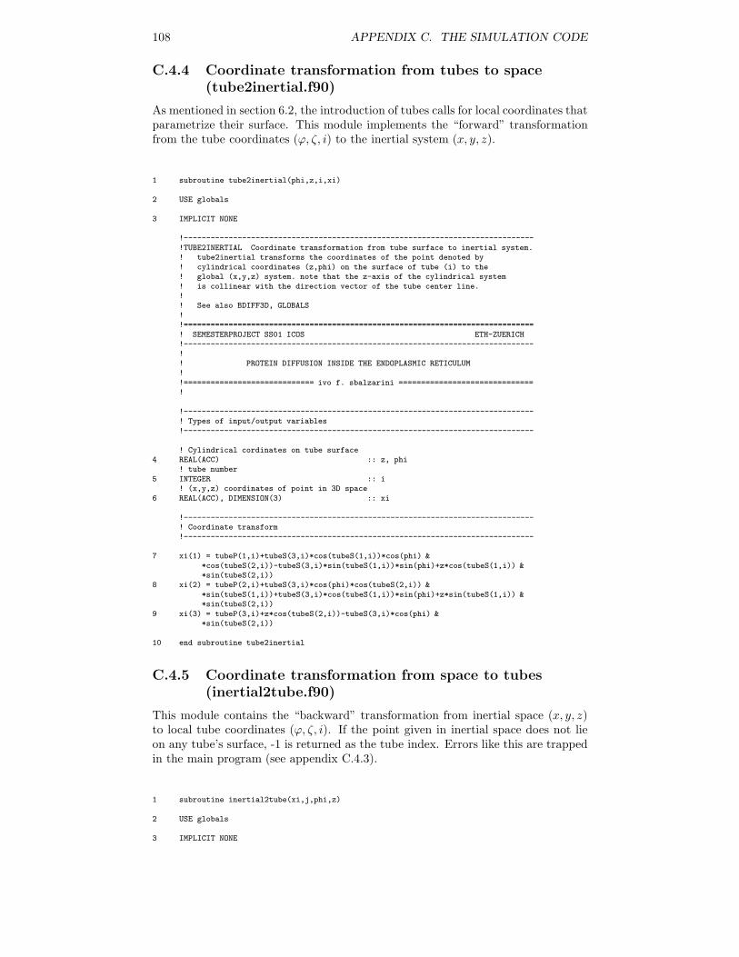
108 APPENDIX C. THE SIMULATION CODE
C.4.4 Coordinate transformation from tubes to space(tube2inertial.f90)
As mentioned in section 6.2, the introduction of tubes calls for local coordinates thatparametrize their surface. This module implements the “forward” transformationfrom the tube coordinates (ϕ, ζ, i) to the inertial system (x, y, z).
1 subroutine tube2inertial(phi,z,i,xi)
2 USE globals
3 IMPLICIT NONE
!------------------------------------------------------------------------------!TUBE2INERTIAL Coordinate transformation from tube surface to inertial system.! tube2inertial transforms the coordinates of the point denoted by! cylindrical coordinates (z,phi) on the surface of tube (i) to the! global (x,y,z) system. note that the z-axis of the cylindrical system! is collinear with the direction vector of the tube center line.!! See also BDIFF3D, GLOBALS!!==============================================================================! SEMESTERPROJECT SS01 ICOS ETH-ZUERICH!------------------------------------------------------------------------------!! PROTEIN DIFFUSION INSIDE THE ENDOPLASMIC RETICULUM!!============================= ivo f. sbalzarini ==============================!
!------------------------------------------------------------------------------! Types of input/output variables!------------------------------------------------------------------------------
! Cylindrical cordinates on tube surface4 REAL(ACC) :: z, phi
! tube number5 INTEGER :: i
! (x,y,z) coordinates of point in 3D space6 REAL(ACC), DIMENSION(3) :: xi
!------------------------------------------------------------------------------! Coordinate transform!------------------------------------------------------------------------------
7 xi(1) = tubeP(1,i)+tubeS(3,i)*cos(tubeS(1,i))*cos(phi) &*cos(tubeS(2,i))-tubeS(3,i)*sin(tubeS(1,i))*sin(phi)+z*cos(tubeS(1,i)) &*sin(tubeS(2,i))
8 xi(2) = tubeP(2,i)+tubeS(3,i)*cos(phi)*cos(tubeS(2,i)) &*sin(tubeS(1,i))+tubeS(3,i)*cos(tubeS(1,i))*sin(phi)+z*sin(tubeS(1,i)) &*sin(tubeS(2,i))
9 xi(3) = tubeP(3,i)+z*cos(tubeS(2,i))-tubeS(3,i)*cos(phi) &*sin(tubeS(2,i))
10 end subroutine tube2inertial
C.4.5 Coordinate transformation from space to tubes(inertial2tube.f90)
This module contains the “backward” transformation from inertial space (x, y, z)to local tube coordinates (ϕ, ζ, i). If the point given in inertial space does not lieon any tube’s surface, -1 is returned as the tube index. Errors like this are trappedin the main program (see appendix C.4.3).
1 subroutine inertial2tube(xi,j,phi,z)
2 USE globals
3 IMPLICIT NONE
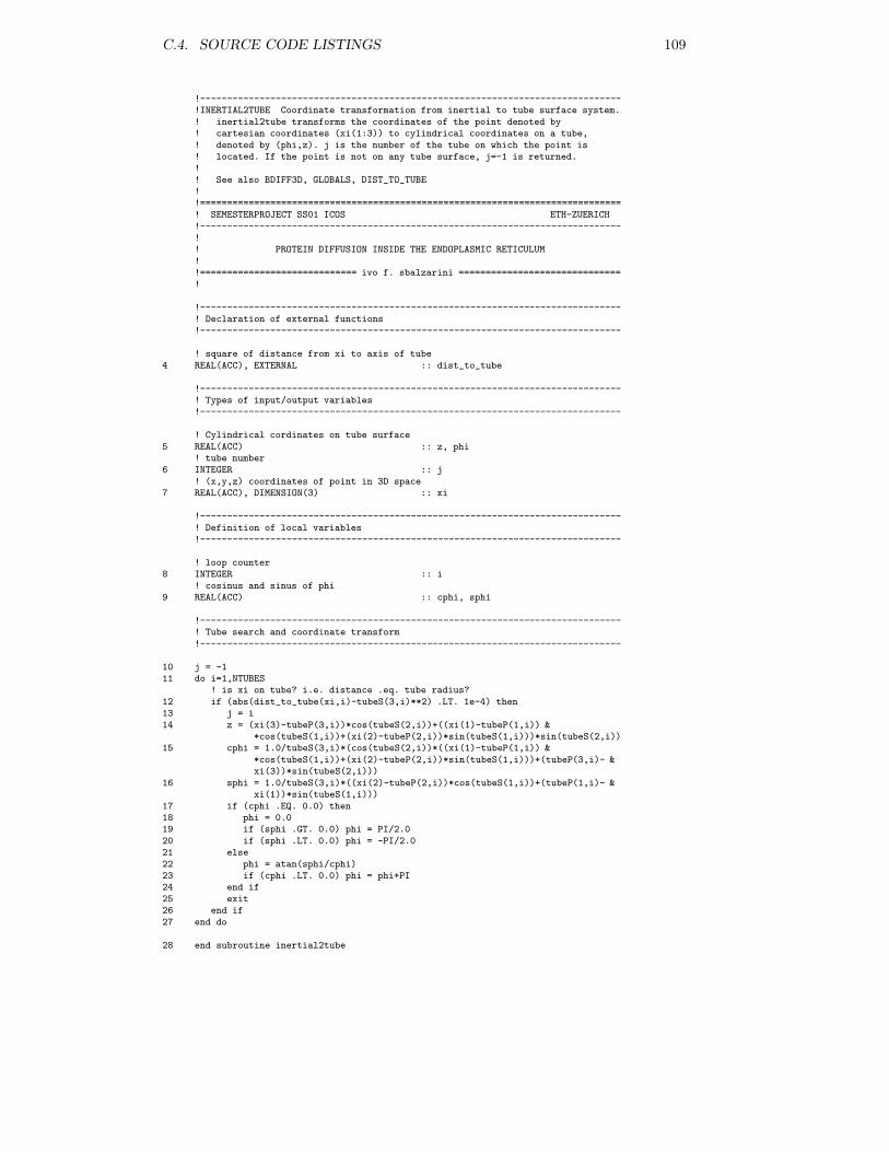
C.4. SOURCE CODE LISTINGS 109
!------------------------------------------------------------------------------!INERTIAL2TUBE Coordinate transformation from inertial to tube surface system.! inertial2tube transforms the coordinates of the point denoted by! cartesian coordinates (xi(1:3)) to cylindrical coordinates on a tube,! denoted by (phi,z). j is the number of the tube on which the point is! located. If the point is not on any tube surface, j=-1 is returned.!! See also BDIFF3D, GLOBALS, DIST_TO_TUBE!!==============================================================================! SEMESTERPROJECT SS01 ICOS ETH-ZUERICH!------------------------------------------------------------------------------!! PROTEIN DIFFUSION INSIDE THE ENDOPLASMIC RETICULUM!!============================= ivo f. sbalzarini ==============================!
!------------------------------------------------------------------------------! Declaration of external functions!------------------------------------------------------------------------------
! square of distance from xi to axis of tube4 REAL(ACC), EXTERNAL :: dist_to_tube
!------------------------------------------------------------------------------! Types of input/output variables!------------------------------------------------------------------------------
! Cylindrical cordinates on tube surface5 REAL(ACC) :: z, phi
! tube number6 INTEGER :: j
! (x,y,z) coordinates of point in 3D space7 REAL(ACC), DIMENSION(3) :: xi
!------------------------------------------------------------------------------! Definition of local variables!------------------------------------------------------------------------------
! loop counter8 INTEGER :: i
! cosinus and sinus of phi9 REAL(ACC) :: cphi, sphi
!------------------------------------------------------------------------------! Tube search and coordinate transform!------------------------------------------------------------------------------
10 j = -111 do i=1,NTUBES
! is xi on tube? i.e. distance .eq. tube radius?12 if (abs(dist_to_tube(xi,i)-tubeS(3,i)**2) .LT. 1e-4) then13 j = i14 z = (xi(3)-tubeP(3,i))*cos(tubeS(2,i))+((xi(1)-tubeP(1,i)) &
*cos(tubeS(1,i))+(xi(2)-tubeP(2,i))*sin(tubeS(1,i)))*sin(tubeS(2,i))15 cphi = 1.0/tubeS(3,i)*(cos(tubeS(2,i))*((xi(1)-tubeP(1,i)) &
*cos(tubeS(1,i))+(xi(2)-tubeP(2,i))*sin(tubeS(1,i)))+(tubeP(3,i)- &xi(3))*sin(tubeS(2,i)))
16 sphi = 1.0/tubeS(3,i)*((xi(2)-tubeP(2,i))*cos(tubeS(1,i))+(tubeP(1,i)- &xi(1))*sin(tubeS(1,i)))
17 if (cphi .EQ. 0.0) then18 phi = 0.019 if (sphi .GT. 0.0) phi = PI/2.020 if (sphi .LT. 0.0) phi = -PI/2.021 else22 phi = atan(sphi/cphi)23 if (cphi .LT. 0.0) phi = phi+PI24 end if25 exit26 end if27 end do
28 end subroutine inertial2tube

110 APPENDIX C. THE SIMULATION CODE
C.4.6 Distance to tube surface(dist to tube.f90)
This small module calculates the square of the orthogonal distance from any pointin space to the center line of a given tube. Its algorithm has been described insection 6.2. The actual distance which would be the square root of its return valueis often not needed since usually comparisons are to be made. To save CPU time,the square of the distance is returned here and the square root is to be taken in thecalling module if needed.
1 function dist_to_tube(xi, jtube)
2 USE globals
3 IMPLICIT NONE
!------------------------------------------------------------------------------!DIST_TO_TUBE returns square of distance of point xi from tube center line.! dist_to_tube returns the square of the distance of the point xi(1:3)! from the center line of tube jtube.!! See also BDIFF3D, GLOBALS!!==============================================================================! SEMESTERPROJECT SS01 ICOS ETH-ZUERICH!------------------------------------------------------------------------------!! PROTEIN DIFFUSION INSIDE THE ENDOPLASMIC RETICULUM!!============================= ivo f. sbalzarini ==============================!
!------------------------------------------------------------------------------! Types of input/output variables!------------------------------------------------------------------------------
! return value: distance4 REAL(ACC) :: dist_to_tube
! tube number5 INTEGER :: jtube
! (x,y,z) coordinates of point in 3D space6 REAL(ACC), DIMENSION(3) :: xi
!------------------------------------------------------------------------------! Types of input/output variables!------------------------------------------------------------------------------
! vector from tube starting point to xi7 REAL(ACC), DIMENSION(3) :: a
! projection onto tube center line8 REAL(ACC) :: pd
!------------------------------------------------------------------------------! Distance calculation!------------------------------------------------------------------------------
! vector from tube starting point to point xi9 a = xi-tubeP(1:3,jtube)
! scalar product: projection of a onto tuber10 pd = dot_product(a,tuber(1:3,jtube))
! square of distance of xi from tube center line11 dist_to_tube = sum(a(:)**2)-pd**2
12 return
13 end function dist_to_tube
C.4.7 Check whether a point is inside the domain(point in domain.f90)
This subroutine checks whether a given point is located inside or outside the com-putational domain. The topological problem of determining “inside” and “outside”
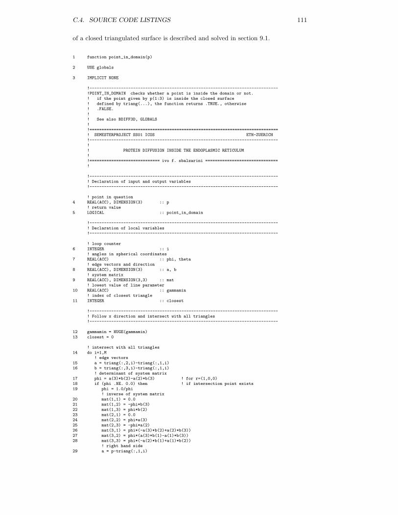
C.4. SOURCE CODE LISTINGS 111
of a closed triangulated surface is described and solved in section 9.1.
1 function point_in_domain(p)
2 USE globals
3 IMPLICIT NONE
!------------------------------------------------------------------------------!POINT_IN_DOMAIN checks whether a point is inside the domain or not.! if the point given by p(1:3) is inside the closed surface! defined by triang(...), the function returns .TRUE., otherwise! .FALSE.!! See also BDIFF3D, GLOBALS!!==============================================================================! SEMESTERPROJECT SS01 ICOS ETH-ZUERICH!------------------------------------------------------------------------------!! PROTEIN DIFFUSION INSIDE THE ENDOPLASMIC RETICULUM!!============================= ivo f. sbalzarini ==============================!
!------------------------------------------------------------------------------! Declaration of input and output variables!------------------------------------------------------------------------------
! point in question4 REAL(ACC), DIMENSION(3) :: p
! return value5 LOGICAL :: point_in_domain
!------------------------------------------------------------------------------! Declaration of local variables!------------------------------------------------------------------------------
! loop counter6 INTEGER :: i
! angles in spherical coordinates7 REAL(ACC) :: phi, theta
! edge vectors and direction8 REAL(ACC), DIMENSION(3) :: a, b
! system matrix9 REAL(ACC), DIMENSION(3,3) :: mat
! lowest value of line parameter10 REAL(ACC) :: gammamin
! index of closest triangle11 INTEGER :: closest
!------------------------------------------------------------------------------! Follow x direction and intersect with all triangles!------------------------------------------------------------------------------
12 gammamin = HUGE(gammamin)13 closest = 0
! intersect with all triangles14 do i=1,M
! edge vectors15 a = triang(:,2,i)-triang(:,1,i)16 b = triang(:,3,i)-triang(:,1,i)
! determinant of system matrix17 phi = a(3)*b(2)-a(2)*b(3) ! for r=(1,0,0)18 if (phi .NE. 0.0) then ! if intersection point exists19 phi = 1.0/phi
! inverse of system matrix20 mat(1,1) = 0.021 mat(1,2) = -phi*b(3)22 mat(1,3) = phi*b(2)23 mat(2,1) = 0.024 mat(2,2) = phi*a(3)25 mat(2,3) = -phi*a(2)26 mat(3,1) = phi*(-a(3)*b(2)+a(2)*b(3))27 mat(3,2) = phi*(a(3)*b(1)-a(1)*b(3))28 mat(3,3) = phi*(-a(2)*b(1)+a(1)*b(2))
! right hand side29 a = p-triang(:,1,i)
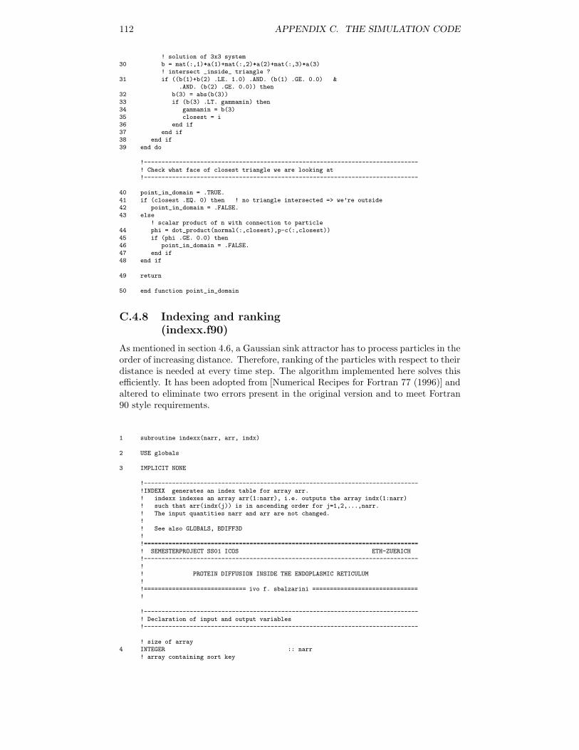
112 APPENDIX C. THE SIMULATION CODE
! solution of 3x3 system30 b = mat(:,1)*a(1)+mat(:,2)*a(2)+mat(:,3)*a(3)
! intersect _inside_ triangle ?31 if ((b(1)+b(2) .LE. 1.0) .AND. (b(1) .GE. 0.0) &
.AND. (b(2) .GE. 0.0)) then32 b(3) = abs(b(3))33 if (b(3) .LT. gammamin) then34 gammamin = b(3)35 closest = i36 end if37 end if38 end if39 end do
!------------------------------------------------------------------------------! Check what face of closest triangle we are looking at!------------------------------------------------------------------------------
40 point_in_domain = .TRUE.41 if (closest .EQ. 0) then ! no triangle intersected => we’re outside42 point_in_domain = .FALSE.43 else
! scalar product of n with connection to particle44 phi = dot_product(normal(:,closest),p-c(:,closest))45 if (phi .GE. 0.0) then46 point_in_domain = .FALSE.47 end if48 end if
49 return
50 end function point_in_domain
C.4.8 Indexing and ranking(indexx.f90)
As mentioned in section 4.6, a Gaussian sink attractor has to process particles in theorder of increasing distance. Therefore, ranking of the particles with respect to theirdistance is needed at every time step. The algorithm implemented here solves thisefficiently. It has been adopted from [Numerical Recipes for Fortran 77 (1996)] andaltered to eliminate two errors present in the original version and to meet Fortran90 style requirements.
1 subroutine indexx(narr, arr, indx)
2 USE globals
3 IMPLICIT NONE
!------------------------------------------------------------------------------!INDEXX generates an index table for array arr.! indexx indexes an array arr(1:narr), i.e. outputs the array indx(1:narr)! such that arr(indx(j)) is in ascending order for j=1,2,...,narr.! The input quantities narr and arr are not changed.!! See also GLOBALS, BDIFF3D!!==============================================================================! SEMESTERPROJECT SS01 ICOS ETH-ZUERICH!------------------------------------------------------------------------------!! PROTEIN DIFFUSION INSIDE THE ENDOPLASMIC RETICULUM!!============================= ivo f. sbalzarini ==============================!
!------------------------------------------------------------------------------! Declaration of input and output variables!------------------------------------------------------------------------------
! size of array4 INTEGER :: narr
! array containing sort key
C.4. SOURCE CODE LISTINGS 113
5 REAL(ACC), DIMENSION(narr) :: arr! array for index table
6 INTEGER, DIMENSION(narr) :: indx
!------------------------------------------------------------------------------! Declaration of parameters!------------------------------------------------------------------------------
7 INTEGER, PARAMETER :: MM = 7! stack size
8 INTEGER, PARAMETER :: NSTACK = 50
!------------------------------------------------------------------------------! Declaration of local variables!------------------------------------------------------------------------------
! loop counters and indices9 INTEGER :: i, indxt, ir, itemp, j10 INTEGER :: jstack, k, l
! stack11 INTEGER, DIMENSION(NSTACK) :: istack12 REAL(ACC) :: a
!------------------------------------------------------------------------------! Algorithm according to Numerical Recipes, pp. 330!------------------------------------------------------------------------------
13 do j=1,narr14 indx(j) = j15 end do
16 jstack = 017 l = 118 ir = narr
19 1 if (ir-l .LT. MM) then20 do j=l+1,ir21 indxt = indx(j)22 a = arr(indxt)23 do i=j-1,1,-124 if (arr(indx(i)) .LE. a) goto 225 indx(i+1) = indx(i)26 end do27 i = 028 2 indx(i+1) = indxt29 end do30 if (jstack .EQ. 0) return31 ir = istack(jstack)32 l = istack(jstack-1)33 jstack = jstack-234 else35 k = (l+ir)/236 itemp = indx(k)37 indx(k) = indx(l+1)38 indx(l+1) = itemp39 if (arr(indx(l+1)) .GT. arr(indx(ir))) then40 itemp = indx(l+1)41 indx(l+1) = indx(ir)42 indx(ir) = itemp43 end if44 if (arr(indx(l)) .GT. arr(indx(ir))) then45 itemp = indx(l)46 indx(l) = indx(ir)47 indx(ir) = itemp48 end if49 if (arr(indx(l+1)) .GT. arr(indx(l))) then50 itemp = indx(l+1)51 indx(l+1) = indx(l)52 indx(l) = itemp53 end if54 i = l+155 j = ir56 indxt = indx(l)57 a = arr(indxt)58 3 continue59 i = i+160 if (arr(indx(i)) .LT. a) goto 361 4 continue62 j = j-163 if (arr(indx(j)) .GT. a) goto 4
114 APPENDIX C. THE SIMULATION CODE
64 if (j .LT. i) goto 565 itemp = indx(i)66 indx(i) = indx(j)67 indx(j) = itemp68 goto 369 5 indx(l) = indx(j)70 indx(j) = indxt71 jstack = jstack+272 if (jstack .GT. NSTACK) pause ’NSTACK too small in indexx’73 if (ir-i+1 .GE. j-1) then74 istack(jstack) = ir75 istack(jstack-1) = i76 ir = j-177 else78 istack(jstack) = j-179 istack(jstack-1) = l80 l = i81 end if82 end if83 goto 1
84 END subroutine indexx
C.4.9 Uniform random number generator(ran2.f)
This is the generating routine for uniformly distributed random numbers between0 and 1. It was taken out of [Numerical Recipes for Fortran 77 (1996)] and the useof the kind parameter ACC for easy accuracy changes was added.
1 FUNCTION ran2(idum_2)
2 USE globals
3 INTEGER idum_2,IA,IM,IQ,IR,NTAB,NDIV4 REAL(ACC) :: ran2,AM,EPS,RNMX5 PARAMETER (IA=16807,IM=2147483647,AM=1./IM,IQ=127773,IR=2836,6 *NTAB=32,NDIV=1+(IM-1)/NTAB,EPS=1.2e-7,RNMX=1.-EPS)
7 INTEGER j,k,iv(NTAB),iy8 SAVE iv,iy9 DATA iv /NTAB*0/, iy /0/10 if (idum_2.le.0.or.iy.eq.0) then11 idum_2=max(-idum_2,1)12 do 11 j=NTAB+8,1,-113 k=idum_2/IQ14 idum_2=IA*(idum_2-k*IQ)-IR*k15 if (idum_2.lt.0) idum_2=idum_2+IM16 if (j.le.NTAB) iv(j)=idum_217 11 continue18 iy=iv(1)19 endif20 k=idum_2/IQ21 idum_2=IA*(idum_2-k*IQ)-IR*k22 if (idum_2.lt.0) idum_2=idum_2+IM23 j=1+iy/NDIV24 iy=iv(j)25 iv(j)=idum_226 ran2=min(AM*iy,RNMX)27 return28 END
C.4.10 Gaussian random number generator(gasdev.f)
This routine implements the Box-Muller algorithm to create Gaussian deviates usingthe uniform random number generator described in the preceding section and anonlinear coordinate transformation.
C.4. SOURCE CODE LISTINGS 115
It was taken out of [Numerical Recipes for Fortran 77 (1996)] with addition of thekind parameter ACC.
1 FUNCTION gasdev(idum_2)
2 USE globals
3 INTEGER idum_24 REAL(ACC) gasdev
! Returns a normally distributed deviate with zero mean and unit variance,! using ran2(idum) as the source of uniform deviates.
5 INTEGER iset6 REAL(ACC) fac,gset,rsq,v1,v2,ran27 SAVE iset,gset8 DATA iset/0/9 IF (iset.EQ.0) THEN10 1 v1=2.*ran2(idum_2)-1.11 v2=2.*ran2(idum_2)-1.12 rsq=v1**2+v2**213 IF(rsq.GE.1..OR.rsq.EQ.0.)GOTO 114 fac=sqrt(-2.*log(rsq)/rsq)15 gset=v1*fac16 gasdev=v2*fac17 iset=118 ELSE19 gasdev=gset20 iset=021 ENDIF22 RETURN23 END