Embed Size (px)
Citation preview
1
On Magnetic Amplifiers in Aircraft Applications
Lars Austrin
ELECTROMAGNETIC ENGINEERING SCHOOL OF ELECTRICAL ENGINEERING
2
ROYAL INSTITUTE OF TECHNOLOGY SWEDEN
Submitted to the School of Electrical Engineering, KTH, in partial fulfillment of the requirements for the degree of
Licentiate of Technology.
Stockholm 2007
Lars Austrin Saab AB, Saab Aerosystems SE-581 88 Linköping Royal Institute of Technology Electromagnetic Engineering SE-100 44 Stockholm Sweden Cover Photo, JAS39A and JAS39B, by: Katsuhiko Tokunaga
Akademisk avhandling som med tillstånd av Kungl Tekniska Högskolan framläggs till offentlig granskning för avläggande av teknologie licentiatexamen 2007-06-08 kl 11.30 i sal H1, Teknikringen 33, Kungl Tekniska Högskolan Stockholm.
TRITA-EE-2007-20
ISSN: 1653-5146 ISBN 978-91-7178-664-7
© Lars Austrin, Stockholm, 2007

3

Abstract
I
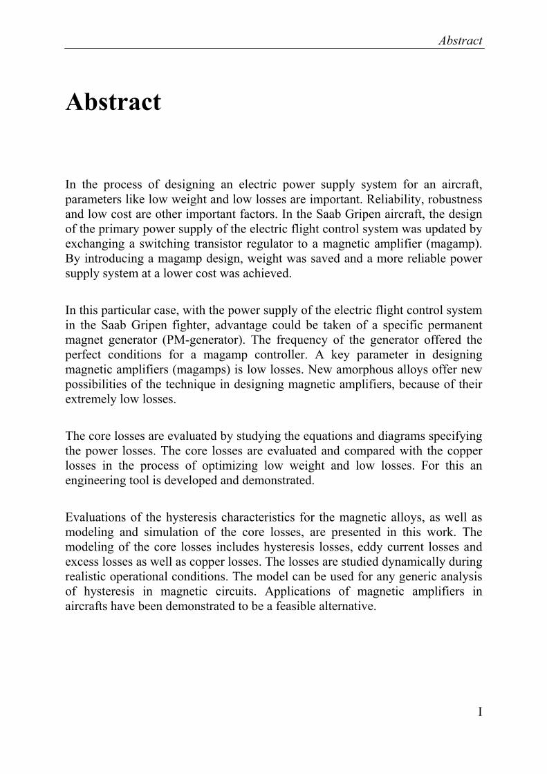
Abstract
In the process of designing an electric power supply system for an aircraft, parameters like low weight and low losses are important. Reliability, robustness and low cost are other important factors. In the Saab Gripen aircraft, the design of the primary power supply of the electric flight control system was updated by exchanging a switching transistor regulator to a magnetic amplifier (magamp). By introducing a magamp design, weight was saved and a more reliable power supply system at a lower cost was achieved.
In this particular case, with the power supply of the electric flight control system in the Saab Gripen fighter, advantage could be taken of a specific permanent magnet generator (PM-generator). The frequency of the generator offered the perfect conditions for a magamp controller. A key parameter in designing magnetic amplifiers (magamps) is low losses. New amorphous alloys offer new possibilities of the technique in designing magnetic amplifiers, because of their extremely low losses.
The core losses are evaluated by studying the equations and diagrams specifying the power losses. The core losses are evaluated and compared with the copper losses in the process of optimizing low weight and low losses. For this an engineering tool is developed and demonstrated.
Evaluations of the hysteresis characteristics for the magnetic alloys, as well as modeling and simulation of the core losses, are presented in this work. The modeling of the core losses includes hysteresis losses, eddy current losses and excess losses as well as copper losses. The losses are studied dynamically during realistic operational conditions. The model can be used for any generic analysis of hysteresis in magnetic circuits. Applications of magnetic amplifiers in aircrafts have been demonstrated to be a feasible alternative.
Keywords
II
Keywords
• Magnetic Amplifier (Magamp) • Amorphous • Power Losses • Control Winding • Self-saturating • Hysteresis • Converter • More Electric Aircraft (MEA) • Inverter • Power-by-Wire • Dymola • Permanent Magnet Generator (PM-generator) • Transformer Rectifier Unit (TRU) • Constant Speed Drive (CSD) • Excess losses or anomalous losses • Modeling • Simulation • Unmanned Aerial Vehicle (UAV)
Acknowledgement
III
Acknowledgements
This work has been supported by many persons from different organizations. First, I would like to express my thanks to my professor, Göran Engdahl, for his inspiration, guidance and experience shared with his students. I would also like to thank professor Roland Eriksson and my colleagues at KTH, Julius Krah, David Ribbenfjärd, Per Pettersson and Mohsen Torabzadeh-Tari for interesting discussions and important contributions as co authors.
To my colleagues at Saab, Eiwe Nilsson, and KG Fransson, I express my thanks for their support and interesting discussions.
The support by Saab management is represented by Lars Borggren, Peter Dickman and my tutor, PhD Birgitta Lantto, as well as the Saab research program directorate represented by Göran Bengtsson. Thank you for making this work possible.
Furthermore I would like to express my thanks to professor Petter Krus, PhD Björn Johansson, and Peter Hallberg for corporative works at LiTH.
Thanks to the sponsor, represented by Curt Eidefeldt, FMV, Erik Prisell, FMV as well as Owe Lyrsell, Lutab, whose support in the field of More Electric Aircraft technology has been essential for this work.
This work was financed by Saab Aerosystems and the Swedish National Aerospace Research Program (NFFP).
I must express my gratitude to my wife, Gun. Without her patience and support, this work would not have been possible. Finally I would express my appreciation to all colleagues, family, and friends who have supported and encouraged me during the process.
Stockholm and Linköping, June 2007 Lars Austrin

Contents
V
Contents
CHAPTER 1 INTRODUCTION................................................................... 1
1.1 BACKGROUND ........................................................................................ 1 1.2 HISTORY................................................................................................. 3 1.3 AIM ........................................................................................................ 8 1.4 OUTLINE OF THE THESIS ....................................................................... 10 1.5 LIST OF PUBLICATIONS......................................................................... 11
CHAPTER 2 THE MAGNETIC SWITCH ............................................... 13
2.1 PRINCIPAL FUNCTION ........................................................................... 13 2.2 MODE OF OPERATION ........................................................................... 17
CHAPTER 3 THE MAGNETIC AMPLIFIER......................................... 19
3.1 TOPOLOGIES ......................................................................................... 19 3.1.1 The Ramey Amplifier....................................................................... 19 3.1.2 The Self Saturating Magamp........................................................... 23 3.1.3 The Three Phase Magnetic Amplifier ............................................. 23
3.2 THE MAGAMP COMPONENTS................................................................ 24 3.2.1 Rectifier Diodes............................................................................... 24 3.2.2 Cores ............................................................................................... 25 3.2.3 Coils................................................................................................. 25 3.2.4 Control Winding.............................................................................. 26
3.3 AVAILABLE ALLOYS ............................................................................ 27 3.4 HEAT TREATMENT - ANNEALING ......................................................... 30 3.5 LOSS MECHANISMS .............................................................................. 31
3.5.1 The Static Hysteresis Losses ........................................................... 32 3.5.2 Eddy Current Losses ....................................................................... 33 3.5.3 Excess Losses .................................................................................. 33 3.5.4 The Total Losses.............................................................................. 33
CHAPTER 4 MAGNETIC AMPLIFIER DEMONSTRATORS ............ 37
4.1 THE MAGNETIC AMPLIFIER DEMONSTRATOR....................................... 37 4.2 THE JAS39 GRIPEN MAGAMP .............................................................. 38
CHAPTER 5 MAGNETIC AMPLIFIER MODELS................................ 43
5.1 EQUIVALENT CIRCUIT OF THE MAGNETIC SWITCH............................... 43
Contents
VI
5.2 THE CORE MODEL................................................................................ 45 5.2.1 The Static Hysteresis Model............................................................ 45 5.2.2 Eddy current and excess loss phenomena....................................... 47 5.2.3 The Equivalent Circuit of a Core Element...................................... 48
5.3 SIMULATION EXAMPLES....................................................................... 49 5.3.1 Magamp Simulation ........................................................................ 49
5.4 ANALYSIS OF LOSSES AND WEIGHT OF A MAGAMP CORE .................... 60 5.4.1 Graphical Analysis Example........................................................... 61
5.5 A PROPOSED ENGINEERING TOOL ........................................................ 66 5.5.1 Input Parameters............................................................................. 68 5.5.2 Dimensioning-Calculation Examples ............................................. 69 5.5.3 Preliminary Interpretations of the Results from the Engineering Tool ......................................................................................................... 73
5.6 CONCLUSIONS ...................................................................................... 74
CHAPTER 6 SYSTEM INTEGRATION IN AIRCRAFT APPLICATIONS............................................................................................... 77
6.1 AIRCRAFT POWER SUPPLY SYSTEMS.................................................... 77 6.2 FUTURE POWER SYSTEMS .................................................................... 79
6.2.1 Skin Effect in Wiring ....................................................................... 80 6.2.2 Increased Impedance in Wiring ...................................................... 82
6.3 FEASIBLE CONCEPTS ............................................................................ 84
CHAPTER 7 CONCLUSIONS AND FUTURE WORK .......................... 89
7.1 CONCLUSIONS ...................................................................................... 89 7.2 FUTURE WORK ..................................................................................... 90
REFERENCES .................................................................................................. 91
LIST OF SYMBOLS......................................................................................... 95
APPENDIX ........................................................................................................ 97
INDEX ................................................................................................................ 98
Introduction Chapter 1
1
Chapter 1
Introduction
1.1 Background
Historically, Magnetic Amplifiers (Magamps) have had an important role for regulation and control of electric power in different applications, especially prior to the use of semiconductors. This technology is attractive in More Electric Aircraft (MEA) systems due to the possibility to achieve a compact, robust and a highly reliable design. Nevertheless the technology is rather unknown, but deserves to be better known and to be used, due to the new possibilities offered. Producers of Switched Mode Power Supply, looking in to the possibility of using magamps in their products, experience that the learning curve to be able to use the technology is a concern [29]. As a part of this, it is important to inform about More Electric Aircraft (MEA) technology and magamps [4].
Magnetic amplifiers are used in the power supply of the Electronic Flight Control System in the Swedish "Gripen" fighter-aircraft. The first flight took place in 1988, and magnetic amplifiers were introduced in 1995. This aircraft is in service since 1997, and is expected to fly until 2040.
The Gripen magamp is designed to be a three-phase voltage regulator. Other applications are found in the Swedish fighter aircraft AJ37 Viggen, where a magamp is used for the excitation of the generator, i.e. for regulation of the main generator output-voltage. First flight, with this magamp in the generator system, took place in 1967. This aircraft was in service between 1971 and 2005.
Chapter 1 Introduction
2
In J 35 Draken, magamps were used for the navigation platform. First flight with this aircraft took place in 1955 and was in service 1959 and was flying until 2005.
Applications of new soft magnetic materials, such as amorphous magnetic alloys, have enabled usage of magnetic amplifier (magamp) technology in the design of competitive electric power regulators. In the process of designing an electric power supply system for an aircraft, parameters like low weight and low losses are important [9]. Reliability, low maintenance and robustness are other important factors. In the Saab Gripen aircraft, the design of the primary power supply of the electric flight control system was updated by exchanging from a switching transistor regulator to a magnetic amplifier (magamp). By introducing a magamp design, weight was saved and a more reliable unit at a lower price was attained.
An electric power supply system for an aircraft is basically specified by Mil-Std-704, which specifies a 28 VDC system, a three-phase 115 VAC, a 400 Hz system, as well as a 270 VDC system. By comparing the weight and size of the generators and transformers, with units of comparable rating for the commercial systems 50/60 Hz, it can be noted that the aircraft units have a significantly lower weight due to the higher frequency. In the particular case with the power supply of the electric flight control system in the Saab Gripen fighter, advantage could be taken of a specific permanent magnet generator (PM-generator), supplying a variable voltage and a variable frequency between 2400 and 4000 Hz. The higher the frequency, the higher is the potential for weight savings. The weight is roughly proportional to the inverse of the frequency [5].
In the trend of More Electric Aircraft designs [9], with a power supply of 270 VDC, the used power-generators commonly work at a higher frequency than 400 Hz. One question is then whether advantage can be taken of a higher operating frequency.
A key parameter in designing magnetic amplifiers (magamps) is low losses. New amorphous alloys are opening up new possibilities of the technique of designing magnetic amplifiers by offering extremely low losses. The core losses can be evaluated by studying the hysteresis loop experimentally and/or by numerical simulations, or by studying equations or diagrams giving the power loss provided by manufacturers. Alternatively, the core losses can by verified in tests, where the losses are evaluated by electric or thermal methods.
Introduction Chapter 1
3
1.2 History
Historically magnetic amplifiers were used in many different power supply applications. The magnetic amplifier is also called the saturable reactor or the transductor. A magnetic amplifier consists of electric and saturable magnetic circuits so interlinked that the reactance of an AC circuit is controlled by an independently applied magnetization. The history of saturable reactors goes back to 1901 when C. F. Burges and B. Frankenfield described different types of control circuits for DC controlled saturable reactors [13]. A very important development phase started 1912-1918 when Ernst Alexanderson showed a method for modulating high frequency alternating currents from one of his alternators so that it could be used for transatlantic radio telephony [13].
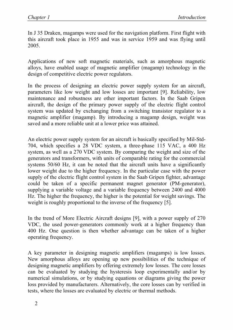
A still preserved part of the history is the transatlantic telegraphic transmitter in Grimeton, south of Gothenburg in Sweden. See Fig. 1. The radio transmitter was made a World Heritage in 2004. The telegraphic transmitter in Grimeton is using the Alexanderson system. The control circuitry is based on a magnetic amplifier. The heart of the power system is an alternating-current generator and a magnetic amplifier, which was developed by the Swedish engineer. The designer Ernst Alexanderson was born in Sweden in 1878. With a degree from the Royal Technical Institute in Stockholm, he joined General Electric 1902. Ernst Alexanderson was employed by Charles Steinmetz at General Electric in Schenectady. Steinmetz [18] is referred to in chapter 3.5.1, due to his work with iron losses. Alexanderson was the holder of 344 patents [15]. He was pioneer in radio, first employed at General Electric in Schenectady and later chief engineer at Radio Corporation of America (RCA).
Chapter 1 Introduction
4
Se Fig. 1. The World Heritage “Grimeton transatlantic telegraphic transmitter”
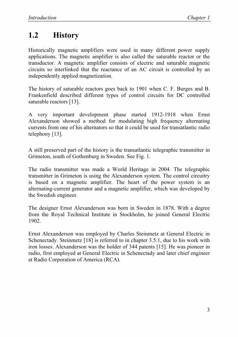
The radio transmitter consists of the following components, the generator, the transformer, the magnetic amplifier, and the capacitors. Other important components are the telegraphic key, and the relay. See Fig. 2, 3 and 4.
Fig. 2. The transformer, T, in the telegraphic transmitter
Introduction Chapter 1
5
The transmitter used a frequency of 17200 Hz, generated by two generators rated at 200 kW. Only one generator remains today. The speed was 2115 rpm with 976 poles. The output from the alternators is routed through a transformer to the antenna. The output voltage from the transformer is 2000V [24].
In the transformer, a magnetisation-winding is shortening the antenna-transformer when no signal shall be transmitted.
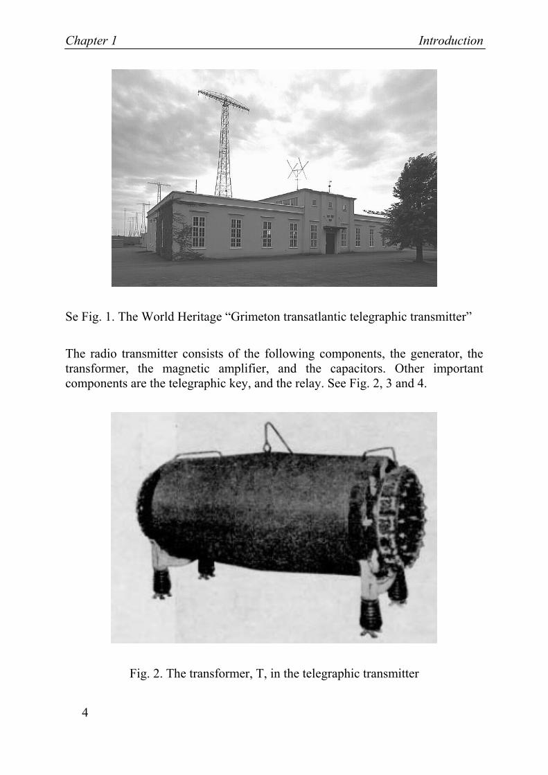
The magnetization winding in the magnetic amplifier is controlled by a telegraphic key, feeding 250 Volt DC to saturate the Magnetic amplifier. The magnetic amplifier has the dimensions of approximately 1.0 x 0.7 x 0.5 m (h x w x d). See Fig. 3.
Fig. 3. The magnetic amplifier in the transmitter in Grimeton
The communication across the Atlantic did not function well during World War I and the need of telegram traffic with United States of America was demanding.
Chapter 1 Introduction
6
The Swedish Parliament therefore decided in 1920 that a Swedish long wave transmitting station and a receiving station should be built under the direction of the Swedish "Telegrafverket".
In the autumn of 1923, the establishment was ready, except for the six 127 meter antenna towers which were delayed one year because of strikes at the ironworks. The towers were placed at intervals of 380 meters with the 46 meter cross-arms on top carrying eight copper wires, which made up the antenna capacitance and the power supply to the six vertical radiating elements.
In December 1924, the radio station Grimeton went into traffic with the call signal SAQ.
In July 1925, the establishment was formally inaugurated by Swedish King Gustaf V and the designer Ernst Alexanderson [21].
Operational Function of the Alexanderson Magamp
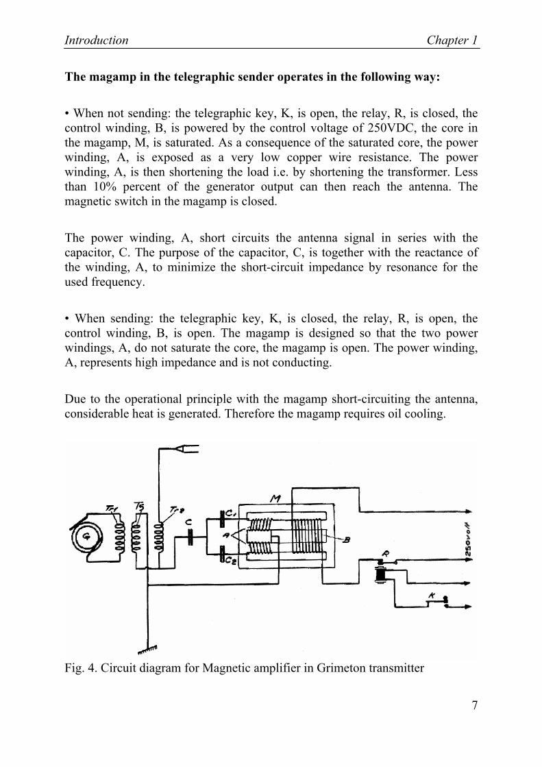
The magnetic amplifier used in the telegraphic transmitter in Grimeton is based on a four-legged core see Fig. 4. The magnetic amplifier operates by switching the mode between saturated and unsaturated state of the magamp M controlled by the telegraphic key [24]. The basic circuit, a parallel connected saturable reactor, is topologically nearby the same as in the basic circuit in Fig. 8.
The signal source is an electric high speed generator, G, giving the frequency 17200 Hz. An ironless transformer, T in Fig 2 and 4, with 2 turns on the primary side is transforming the generator output power to 2000 V and 100 A. The magamp with the power winding, A, short-circuits the antenna by short-circuiting the transformer secondary winding, S in Fig 4, when no signal shall be transmitted.
The magamp, M in Fig. 4, is based on a four leg core with a power winding, A, and a control winding, B. The winding, A, consists of two anti parallel windings.
Introduction Chapter 1
7
The magamp in the telegraphic sender operates in the following way:
• When not sending: the telegraphic key, K, is open, the relay, R, is closed, the control winding, B, is powered by the control voltage of 250VDC, the core in the magamp, M, is saturated. As a consequence of the saturated core, the power winding, A, is exposed as a very low copper wire resistance. The power winding, A, is then shortening the load i.e. by shortening the transformer. Less than 10% percent of the generator output can then reach the antenna. The magnetic switch in the magamp is closed.
The power winding, A, short circuits the antenna signal in series with the capacitor, C. The purpose of the capacitor, C, is together with the reactance of the winding, A, to minimize the short-circuit impedance by resonance for the used frequency.
• When sending: the telegraphic key, K, is closed, the relay, R, is open, the control winding, B, is open. The magamp is designed so that the two power windings, A, do not saturate the core, the magamp is open. The power winding, A, represents high impedance and is not conducting.
Due to the operational principle with the magamp short-circuiting the antenna, considerable heat is generated. Therefore the magamp requires oil cooling.
Fig. 4. Circuit diagram for Magnetic amplifier in Grimeton transmitter
Chapter 1 Introduction
8
The purpose of the capacitors, C1, and, C2, is to block the low frequency signal initiated from the telegraphic key, K.
One reason of the increased interest in magnetic amplifiers was the successful German technical development regarding various military applications, especially for naval fire-control systems, as such for the heavy cruiser "Prins Eugen" [13].
Important Swedish contributions were made by ASEA and inventers like U. Lamm, S.E. Hedström, and B. Nordfeldt [13].
Another interesting magamp application is a Stereo HiFi amplifier based on magnetic amplifiers offered to the market during a few years in the mid eighties by Lundahl Transformers [25]. The designer, Lars Lundahl, based the design on Ramey amplifiers, see Fig. 13. During a visit to Lundahl Transformers in 2004, the author had the opportunity to enjoy the excellent sound of his Stereo HiFi magnetic amplifier [49].
1.3 Aim
The trend in More Electric Aircraft technology is very much driven towards a simplification of the systems and to avoid complex mechanical systems. The other side of the coin might be huge and complex electronic power systems. The power electronic systems are expected to offer system simplification and advantages like a simplified installation. Nevertheless, new concerns arise due to the indicated required power levels of 1 MW of electric power in future commercial aircraft. These power levels stress the importance of reliable and rugged electric power systems.
One important question then is if the magamp technology can find new applications to meet these new requirements in future aircraft systems.
The following topics regarding the exploration of the potential of magnetic amplifiers are described in this thesis.
Introduction Chapter 1
9
• Operation principles
The aim is, to review and analyze the basic circuitry [1] of the magnetic amplifier, based on a one-phase circuit extended to a three-phase circuit and to review different principles of operation.
• Simulation models
The aim is, is to study losses in a three-phase magamp including copper and core losses by simulating the hysteresis characteristics for amorphous magnetic alloys. The losses and the efficiency of the magamp are studied by modeling and simulation of the cores, operating in a three-phase circuit.
The presented model includes static hysteresis, classical eddy currents, and excess losses [6].
Thereby power losses can be evaluated, which enables an optimization of the design.
The use of the hysteresis models to estimate the static and hysteresis loss and excess losses [6, 7] of core material is demonstrated. The losses and the power-density [kW/kg] can thus also be evaluated.
• Evaluation tools
The aim is, to get an engineering tool for analyzing weight and volume [2]. Impact on weight and performance as a function of different magnetic material and operating frequency, are studied. The demonstrated modeling approach is considered to be one important dimensioning tool regarding future development of reliable devices for power management in MEA systems.
Power-density is of vital importance in an aircraft application. This implies the need for analyzing tools, stressing the limits of the current density, as well as optimising the chosen soft magnetic materials, regarding flux density B [T] and core losses.
Chapter 1 Introduction
10
• System integration
The aim is, to study a complete system with magnetic amplifier applications in an aircraft installation.
1.4 Outline of the Thesis
Chapter 1. The Introduction; gives a historical background as well as the motivation of this work on Magnetic Amplifiers.
Chapter 2. The Magnetic Switch; describes the fundamental parts of the magnetic amplifier, i.e. the cores and the copper windings. This gives a basic insight in the operational principles and design of a magnetic amplifier.
Chapter 3. The Magnetic Amplifier; describes how the magnetic switches in chapter 2 can be used in operating units. Normally a three phase magnetic amplifier is designed by three one-phase magamps connected to a six pulse rectifier bridge, giving a total of 12 rectifying diodes. The presented three phase magamp circuit, with 6 rectifying diodes, represents a simplification used in this work. Power circuits and available components, as well as some design considerations are also presented.
Chapter 4. Magnetic Amplifier Demonstrators; describes the author’s work with the design of the magamp demonstrator and the final production unit for the JAS39 fighter, as produced by Euro Atlas in Bremen.
Chapter 5. Magnetic Amplifier Models; a three phase magamp model is implemented in the simulation program package Dymola. This model was used to study the losses in a magamp application is to be able to estimate the losses for different operating frequencies, and is able to manage the nonlinear magnetic properties during transition from non-saturated to a saturated state of the core. Important contributions to the setup of this model were done by D. Ribbenfjärd and G. Engdahl.
An engineering tool for conceptual design of magnetic amplifier is also described in this chapter. The developed tool is based on core loss data supplied
Introduction Chapter 1
11
by the producers. These data, graphically presented for different materials have been expressed as equations for use in the engineering tool. A number of test examples show that a magamp design can be optimized for low losses or low weight. By choosing the right core material for a given operating frequency at a certain power rating, a design with coinciding weight and loss minima also can be achieved. A loss model of the core material that includes static hysteresis, eddy current and excess eddy currents is presented.
Chapter 6. Systems Integration in Aircraft Application; this chapter describes the system integration in aircraft applications. Possible concepts for future power generation and distribution system are described and analyzed with regard to frequency.
Chapter 7. Conclusion and Future work. Concludes the results and summarizes ideas for future work.
1.5 List of Publications
The following articles serve as a base for this thesis work:
[1] L. Austrin, J.H. Krah and G. Engdahl: “A Modeling Approach of a Magnetic Amplifier”. Proc. of the International Conference of Magnetism, Rome, Italy, 27th July-1st August, 2003.
[2] L. Austrin, and G. Engdahl: “Modeling of a Three-phase Magnetic Amplifier”. Proc. of the 24th Congress of the International Council of the Aeronatical Science, Yokohama, Japan, 29th August-3rd September 2004.
[3] B Johansson, L Austrin, G Engdahl, P Krus: Tools and Methodology for Collaborative Systems Design Applied on More Electric Aircraft. Proc. ICAS 2004, Yokohama, Japan, 29th August-3rd September 2004.
[4] L. Austrin, J. Hansson: New Electric Components for Aircrafts. Flygteknik, Proc. Flygteknik, Oktober 18-19, 2004 Stockholm (In Swedish).
[5] P. Krus, B. Johansson, L. Austrin: “Concept Optimization of Aircraft Systems Using Scaling Models”. Proc. Recent Advances in Aerospace Actuation Systems and Components, November 24-26, 2004 Toulouse, France.
Chapter 1 Introduction
12
[6] L. Austrin, D. Ribbenfjärd, G. Engdahl: “Simulation of a Magnetic Amplifier Circuit Including Hysteresis”. Digest for Intermag. Nagoya, Japan, April 2005.
[7] L. Austrin, D. Ribbenfjärd, G. Engdahl: “Simulation of a Magnetic Amplifier Circuit Including Hysteresis”. IEEE transactions, to be published.
[8] Peter Hallberg, Lars Austrin, Petter Krus: “Low Cost Demonstrator as a Mean for Rapid Product Realization with an Electric Motorcycle Application”. Proceedings of IDETC/CIE 2005.
The Magnetic Switch Chapter 2
13
Chapter 2
The Magnetic Switch
In the previous chapter the concept magnetic amplifier (magamp) is used consequently and describes the complete unit including the magnetic elements, all required components for regulation and control, as well as rectifiers. The magnetic elements are based on copper and magnetic cores. To better clarify the operational function of the magnetic elements we hereby introduce the concept “magnetic switch”.
The concept “magnetic switch” describes the operational function of how the magnetic element can work as a switch.
2.1 Principal Function
The operation of a magnetic switch in a magamp is based on switching between unsaturated and saturated state of a magnetic core, see Fig. 5. When the core is saturated and the magnetic switch is conducting, the switch is on. During the following half cycle the magnetic switch can be reset to an unsaturated state such that it is not conducting.
Normally a magnetic switch operates with alternating current in the power winding and direct current in the control winding.
The magnetic switch can be designed with one core, equipped with a power winding and a control winding, see Fig. 5. The problem with this design is that it will operate like a transformer. This implies that the load current transforms a significant current to the control winding and the control circuit [14].
Chapter 2 The Magnetic Switch
14
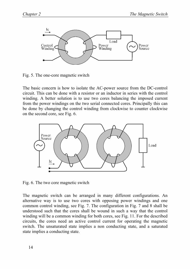
Fig. 5. The one-core magnetic switch
The basic concern is how to isolate the AC-power source from the DC-control circuit. This can be done with a resistor or an inductor in series with the control winding. A better solution is to use two cores balancing the imposed current from the power windings on the two serial connected cores. Principally this can be done by changing the control winding from clockwise to counter clockwise on the second core, see Fig. 6.
Fig. 6. The two core magnetic switch
The magnetic switch can be arranged in many different configurations. An alternative way is to use two cores with opposing power windings and one common control winding, see Fig. 7. The configuration in Fig. 7 and 8 shall be understood such that the cores shall be wound in such a way that the control winding will be a common winding for both cores, see Fig. 11. For the described circuits, the cores need an active control current for operating the magnetic switch. The unsaturated state implies a non conducting state, and a saturated state implies a conducting state.
The Magnetic Switch Chapter 2
15
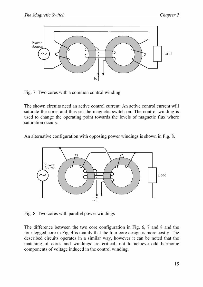
Fig. 7. Two cores with a common control winding
The shown circuits need an active control current. An active control current will saturate the cores and thus set the magnetic switch on. The control winding is used to change the operating point towards the levels of magnetic flux where saturation occurs.
An alternative configuration with opposing power windings is shown in Fig. 8.
Fig. 8. Two cores with parallel power windings
The difference between the two core configuration in Fig. 6, 7 and 8 and the four legged core in Fig. 4 is mainly that the four core design is more costly. The described circuits operates in a similar way, however it can be noted that the matching of cores and windings are critical, not to achieve odd harmonic components of voltage induced in the control winding.
Chapter 2 The Magnetic Switch
16
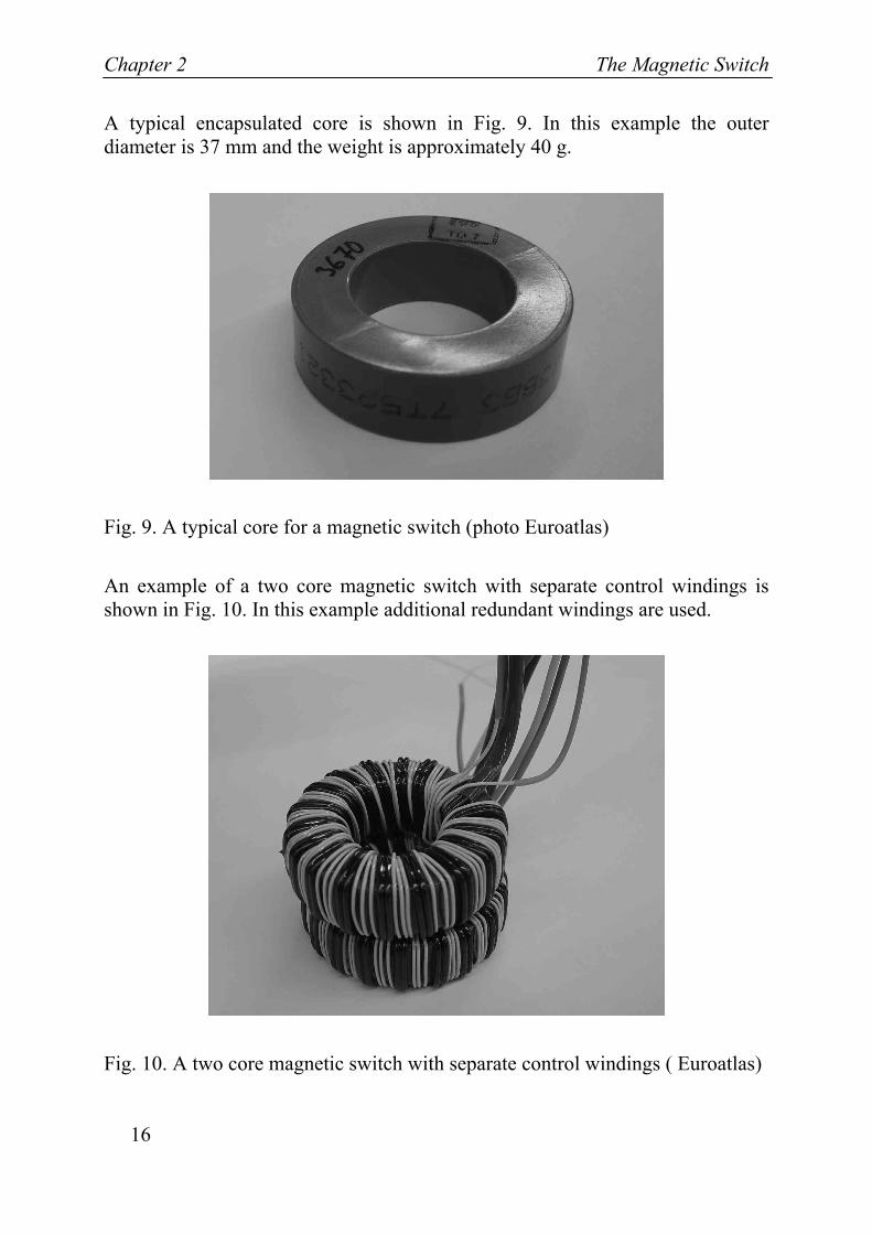
A typical encapsulated core is shown in Fig. 9. In this example the outer diameter is 37 mm and the weight is approximately 40 g.
Fig. 9. A typical core for a magnetic switch (photo Euroatlas)
An example of a two core magnetic switch with separate control windings is shown in Fig. 10. In this example additional redundant windings are used.
Fig. 10. A two core magnetic switch with separate control windings ( Euroatlas)
The Magnetic Switch Chapter 2
17
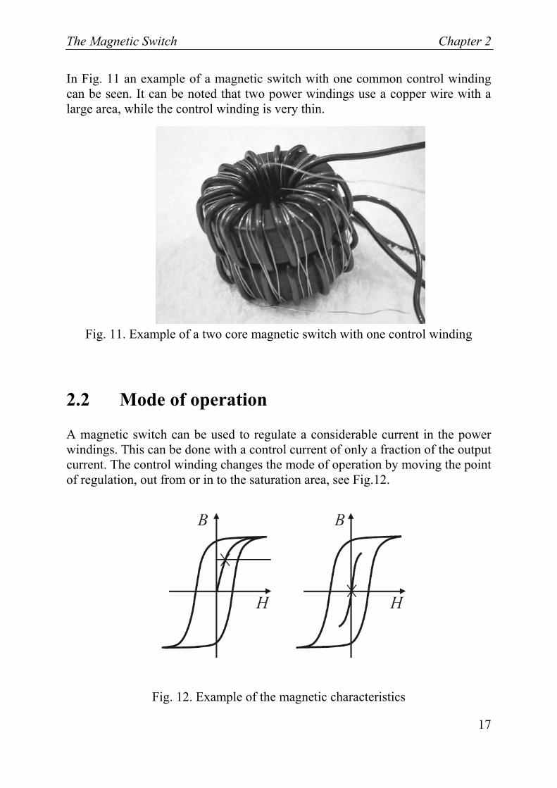
In Fig. 11 an example of a magnetic switch with one common control winding can be seen. It can be noted that two power windings use a copper wire with a large area, while the control winding is very thin.
Fig. 11. Example of a two core magnetic switch with one control winding
2.2 Mode of operation
A magnetic switch can be used to regulate a considerable current in the power windings. This can be done with a control current of only a fraction of the output current. The control winding changes the mode of operation by moving the point of regulation, out from or in to the saturation area, see Fig.12.
Fig. 12. Example of the magnetic characteristics
Chapter 2 The Magnetic Switch
18
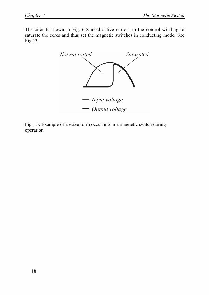
The circuits shown in Fig. 6-8 need active current in the control winding to saturate the cores and thus set the magnetic switches in conducting mode. See Fig.13.
Fig. 13. Example of a wave form occurring in a magnetic switch during operation
The Magnetic Amplifier Chapter 3
19
Chapter 3
The Magnetic Amplifier
The expression magnetic amplifier (magamp) is used to describe the complete unit including the magnetic elements, all required components for regulation and control, as well as rectifiers.
3.1 Topologies
The magnetic amplifier comprises circuits shown in Fig. 6-8, with rectifying diodes such that rectified load-current saturates the cores. The magnetic switches will be set in a conducting mode until the saturation is removed by currents in the control windings.
The self-saturating magnetic amplifier will thus need control currents to take their cores out of saturation.
3.1.1 The Ramey Amplifier The Ramey Amplifier, or with the alternative name, the “flux reset” magamp, is a voltage controlled magnetic amplifier. The magamp is supplied by the AC power source, US, and is feeding the load, RL. The magamp consists of a single wound core, M, in series with a rectifier diod and an inductor, L. The purpose of the inductor, L together with the capacitor, C, and the free wheeling diode, D, is to filter the output voltage.
Chapter 3 The Magnetic Amplifier
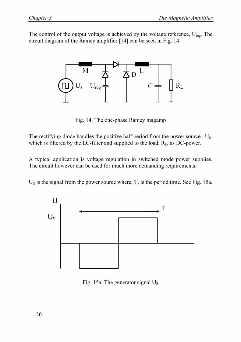
20
The control of the output voltage is achieved by the voltage reference, Ureg. The circuit diagram of the Ramey amplifier [14] can be seen in Fig. 14.
Fig. 14. The one-phase Ramey magamp
The rectifying diode handles the positive half period from the power source , US, which is filtered by the LC-filter and supplied to the load, RL, as DC-power.
A typical application is voltage regulation in switched mode power supplies. The circuit however can be used for much more demanding requirements.
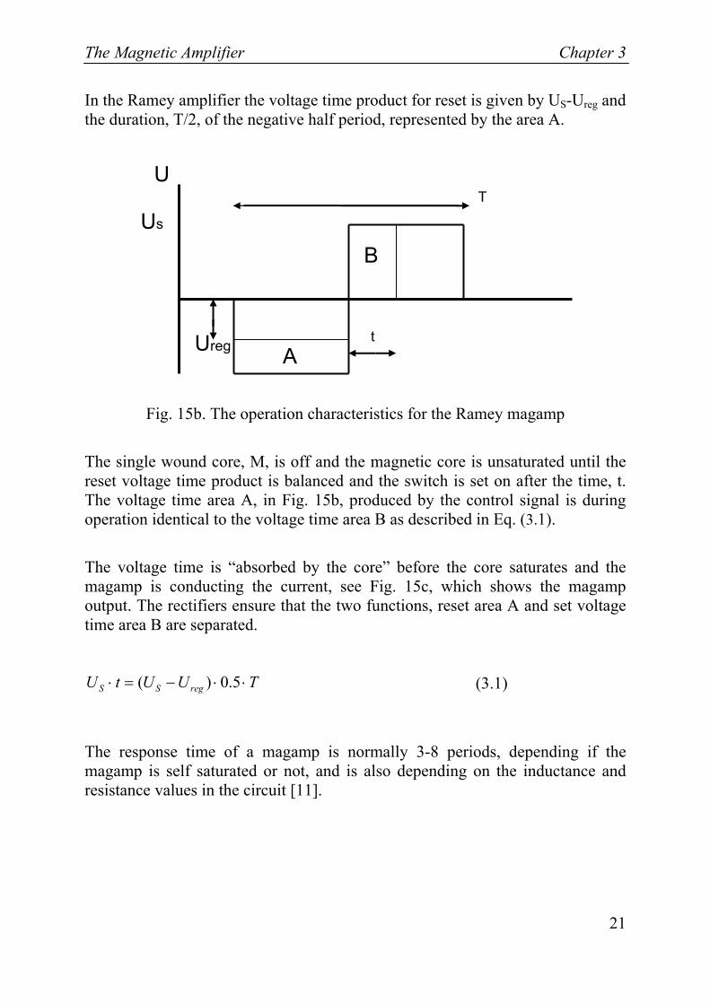
US is the signal from the power source where, T, is the period time. See Fig. 15a.
Fig. 15a. The generator signal US
Us
TU
D
The Magnetic Amplifier Chapter 3
21
In the Ramey amplifier the voltage time product for reset is given by US-Ureg and the duration, T/2, of the negative half period, represented by the area A.
Fig. 15b. The operation characteristics for the Ramey magamp
The single wound core, M, is off and the magnetic core is unsaturated until the reset voltage time product is balanced and the switch is set on after the time, t. The voltage time area A, in Fig. 15b, produced by the control signal is during operation identical to the voltage time area B as described in Eq. (3.1).
The voltage time is “absorbed by the core” before the core saturates and the magamp is conducting the current, see Fig. 15c, which shows the magamp output. The rectifiers ensure that the two functions, reset area A and set voltage time area B are separated.
TUUtU regSS ⋅⋅−=⋅ 5.0)( (3.1)
The response time of a magamp is normally 3-8 periods, depending if the magamp is self saturated or not, and is also depending on the inductance and resistance values in the circuit [11].
Us
t
T
Ureg A
B
U
Chapter 3 The Magnetic Amplifier
22
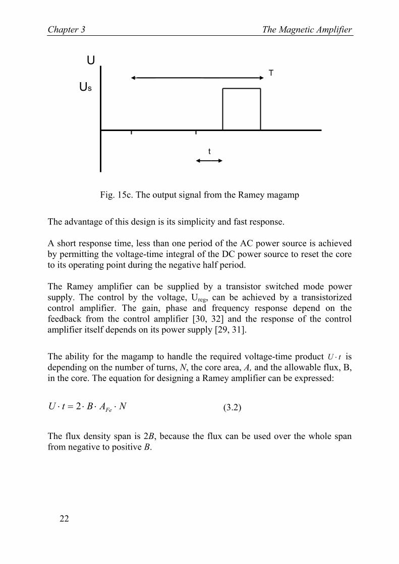
Fig. 15c. The output signal from the Ramey magamp
The advantage of this design is its simplicity and fast response. A short response time, less than one period of the AC power source is achieved by permitting the voltage-time integral of the DC power source to reset the core to its operating point during the negative half period. The Ramey amplifier can be supplied by a transistor switched mode power supply. The control by the voltage, Ureg, can be achieved by a transistorized control amplifier. The gain, phase and frequency response depend on the feedback from the control amplifier [30, 32] and the response of the control amplifier itself depends on its power supply [29, 31].
The ability for the magamp to handle the required voltage-time product tU ⋅ is depending on the number of turns, N, the core area, A, and the allowable flux, B, in the core. The equation for designing a Ramey amplifier can be expressed:
NABtU Fe ⋅⋅⋅=⋅ 2 (3.2)
The flux density span is 2B, because the flux can be used over the whole span from negative to positive B.
Us
t
TU
The Magnetic Amplifier Chapter 3
23
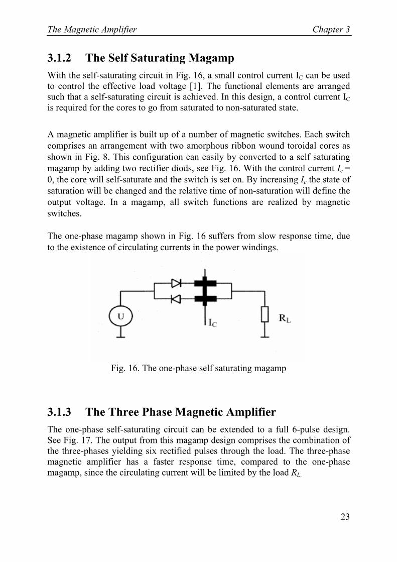
3.1.2 The Self Saturating Magamp With the self-saturating circuit in Fig. 16, a small control current IC can be used to control the effective load voltage [1]. The functional elements are arranged such that a self-saturating circuit is achieved. In this design, a control current IC is required for the cores to go from saturated to non-saturated state.
A magnetic amplifier is built up of a number of magnetic switches. Each switch comprises an arrangement with two amorphous ribbon wound toroidal cores as shown in Fig. 8. This configuration can easily by converted to a self saturating magamp by adding two rectifier diods, see Fig. 16. With the control current Ic = 0, the core will self-saturate and the switch is set on. By increasing Ic the state of saturation will be changed and the relative time of non-saturation will define the output voltage. In a magamp, all switch functions are realized by magnetic switches. The one-phase magamp shown in Fig. 16 suffers from slow response time, due to the existence of circulating currents in the power windings.
Fig. 16. The one-phase self saturating magamp
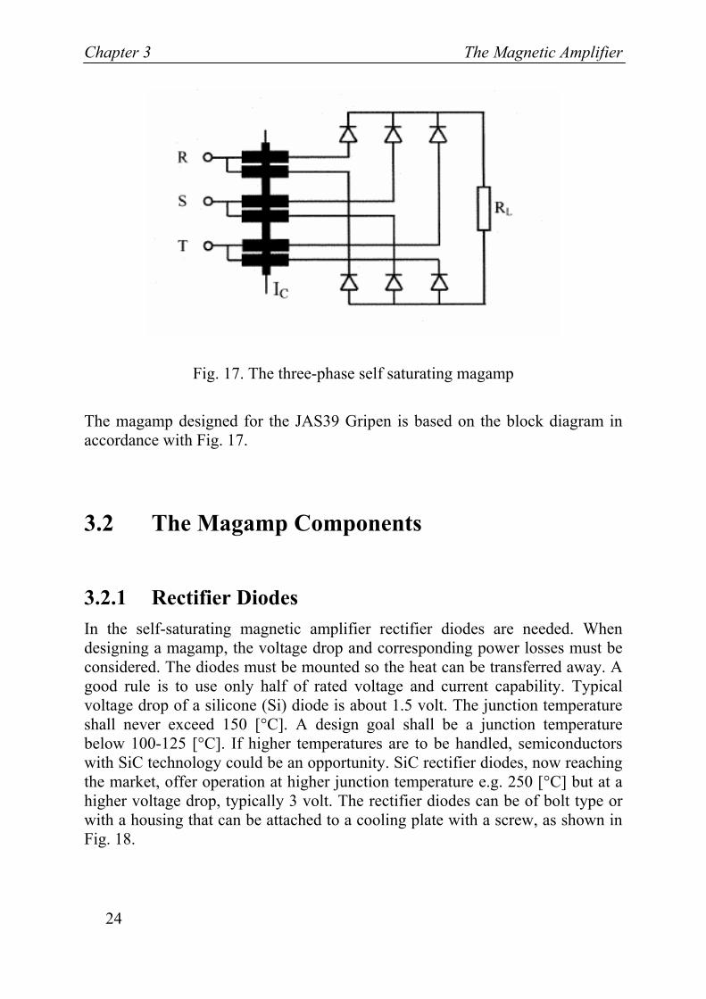
3.1.3 The Three Phase Magnetic Amplifier The one-phase self-saturating circuit can be extended to a full 6-pulse design. See Fig. 17. The output from this magamp design comprises the combination of the three-phases yielding six rectified pulses through the load. The three-phase magnetic amplifier has a faster response time, compared to the one-phase magamp, since the circulating current will be limited by the load RL.
Chapter 3 The Magnetic Amplifier
24
Fig. 17. The three-phase self saturating magamp
The magamp designed for the JAS39 Gripen is based on the block diagram in accordance with Fig. 17.
3.2 The Magamp Components
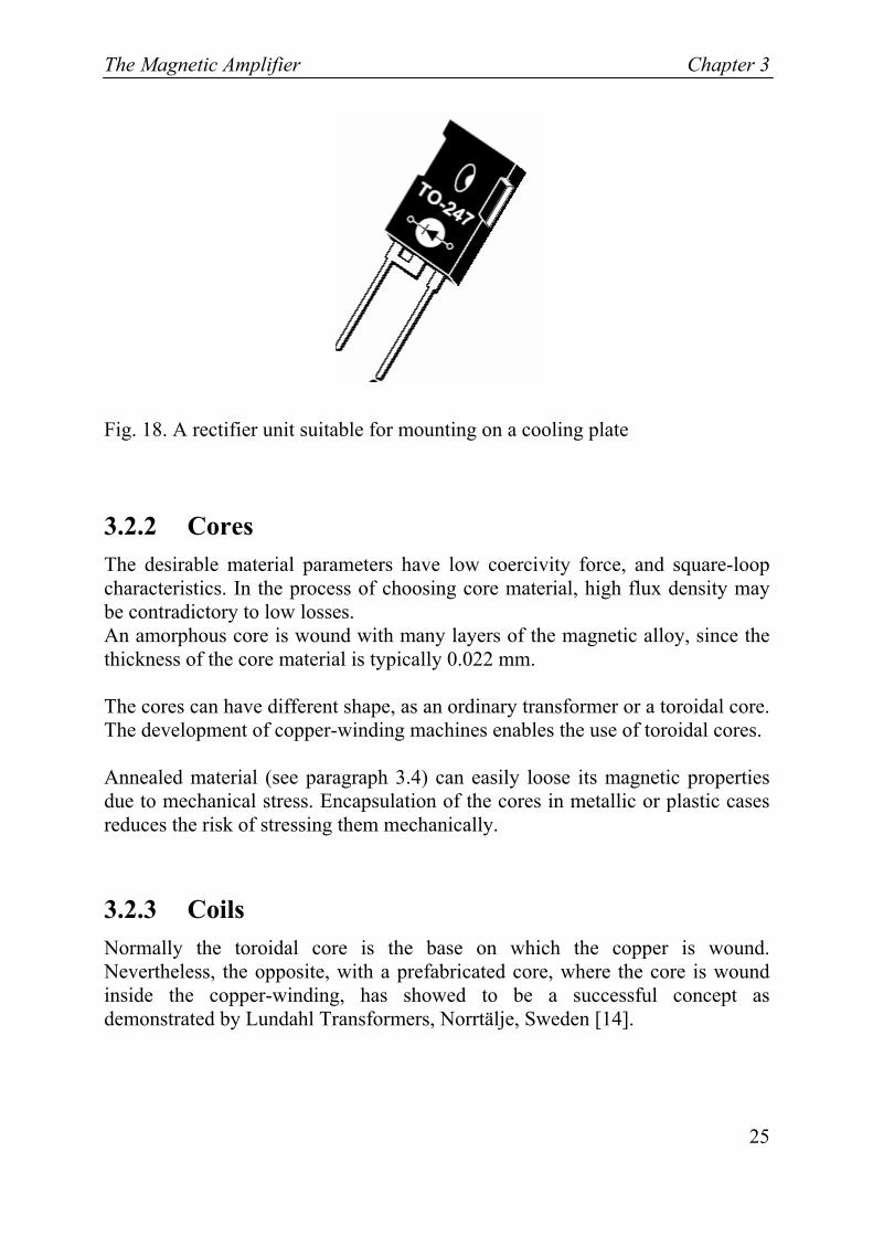
3.2.1 Rectifier Diodes In the self-saturating magnetic amplifier rectifier diodes are needed. When designing a magamp, the voltage drop and corresponding power losses must be considered. The diodes must be mounted so the heat can be transferred away. A good rule is to use only half of rated voltage and current capability. Typical voltage drop of a silicone (Si) diode is about 1.5 volt. The junction temperature shall never exceed 150 [°C]. A design goal shall be a junction temperature below 100-125 [°C]. If higher temperatures are to be handled, semiconductors with SiC technology could be an opportunity. SiC rectifier diodes, now reaching the market, offer operation at higher junction temperature e.g. 250 [°C] but at a higher voltage drop, typically 3 volt. The rectifier diodes can be of bolt type or with a housing that can be attached to a cooling plate with a screw, as shown in Fig. 18.
The Magnetic Amplifier Chapter 3
25
Fig. 18. A rectifier unit suitable for mounting on a cooling plate
3.2.2 Cores The desirable material parameters have low coercivity force, and square-loop characteristics. In the process of choosing core material, high flux density may be contradictory to low losses. An amorphous core is wound with many layers of the magnetic alloy, since the thickness of the core material is typically 0.022 mm. The cores can have different shape, as an ordinary transformer or a toroidal core. The development of copper-winding machines enables the use of toroidal cores. Annealed material (see paragraph 3.4) can easily loose its magnetic properties due to mechanical stress. Encapsulation of the cores in metallic or plastic cases reduces the risk of stressing them mechanically.
3.2.3 Coils Normally the toroidal core is the base on which the copper is wound. Nevertheless, the opposite, with a prefabricated core, where the core is wound inside the copper-winding, has showed to be a successful concept as demonstrated by Lundahl Transformers, Norrtälje, Sweden [14].
Chapter 3 The Magnetic Amplifier
26
3.2.4 Control Winding The advantage of magnetic amplifiers is that large amplification can be achieved, and thus a thin control wire can be used. Other advantages can be the galvanic separation between the power source and the control winding, as well as the option with redundant control wiring.
The control of the magnetic amplifiers is easily attained by transistor circuits. In reference [33] a control circuit for a Ramey amplifier, which is minimizing the unwanted magamp reset signal is presented. This expands its controllable output signal.
A core with a large cross-sectional area and a short magnetic flux path length effectively yields a huge control gain [38] that can be in the order of 1:1000.
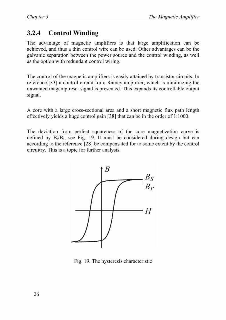
The deviation from perfect squareness of the core magnetization curve is defined by Br/Bs, see Fig. 19. It must be considered during design but can according to the reference [28] be compensated for to some extent by the control circuitry. This is a topic for further analysis.
Fig. 19. The hysteresis characteristic
The Magnetic Amplifier Chapter 3
27
3.3 Available Alloys
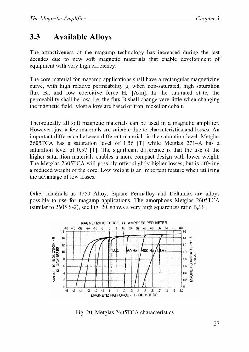
The attractiveness of the magamp technology has increased during the last decades due to new soft magnetic materials that enable development of equipment with very high efficiency. The core material for magamp applications shall have a rectangular magnetizing curve, with high relative permeability µr when non-saturated, high saturation flux Bs, and low coercitive force Hc [A/m]. In the saturated state, the permeability shall be low, i.e. the flux B shall change very little when changing the magnetic field. Most alloys are based or iron, nickel or cobalt.
Theoretically all soft magnetic materials can be used in a magnetic amplifier. However, just a few materials are suitable due to characteristics and losses. An important difference between different materials is the saturation level. Metglas 2605TCA has a saturation level of 1.56 [T] while Metglas 2714A has a saturation level of 0.57 [T]. The significant difference is that the use of the higher saturation materials enables a more compact design with lower weight. The Metglas 2605TCA will possibly offer slightly higher losses, but is offering a reduced weight of the core. Low weight is an important feature when utilizing the advantage of low losses.
Other materials as 4750 Alloy, Square Permalloy and Deltamax are alloys possible to use for magamp applications. The amorphous Metglas 2605TCA (similar to 2605 S-2), see Fig. 20, shows a very high squareness ratio Br/Bs.
Fig. 20. Metglas 2605TCA characteristics
Chapter 3 The Magnetic Amplifier
28
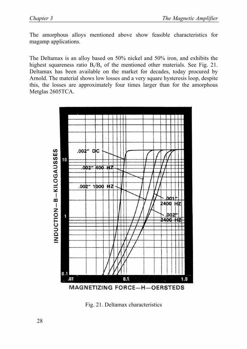
The amorphous alloys mentioned above show feasible characteristics for magamp applications.
The Deltamax is an alloy based on 50% nickel and 50% iron, and exhibits the highest squareness ratio Br/Bs of the mentioned other materials. See Fig. 21. Deltamax has been available on the market for decades, today procured by Arnold. The material shows low losses and a very square hysteresis loop, despite this, the losses are approximately four times larger than for the amorphous Metglas 2605TCA.
Fig. 21. Deltamax characteristics
The Magnetic Amplifier Chapter 3
29
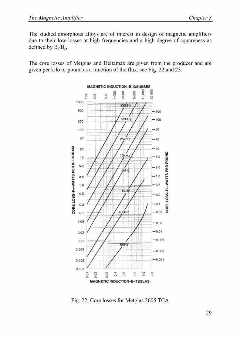
The studied amorphous alloys are of interest in design of magnetic amplifiers due to their low losses at high frequencies and a high degree of squareness as defined by Br/Bs,
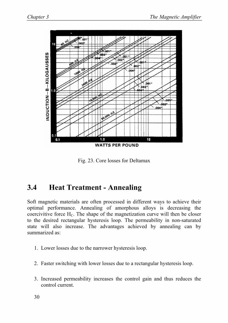
The core losses of Metglas and Deltamax are given from the producer and are given per kilo or pound as a function of the flux, see Fig. 22 and 23.
Fig. 22. Core losses for Metglas 2605 TCA
Chapter 3 The Magnetic Amplifier
30
Fig. 23. Core losses for Deltamax
3.4 Heat Treatment - Annealing
Soft magnetic materials are often processed in different ways to achieve their optimal performance. Annealing of amorphous alloys is decreasing the coercivitive force HC. The shape of the magnetization curve will then be closer to the desired rectangular hysteresis loop. The permeability in non-saturated state will also increase. The advantages achieved by annealing can by summarized as:
1. Lower losses due to the narrower hysteresis loop.
2. Faster switching with lower losses due to a rectangular hysteresis loop.
3. Increased permeability increases the control gain and thus reduces the control current.
The Magnetic Amplifier Chapter 3
31
The detailed annealing process might vary between different alloys and different suppliers. For information a comprehensive annealing process used by Saab is hereby summarized, see Table 1. Annealing is normally performed in an oven with an inert gas, where it is possible to magnetize the cores with a DC-current.
Table 1. Annealing data used by Saab
Time for annealing 1h
Temperature 350-400 [°C]
Magnetic field. 800 [A/m]
3.5 Loss Mechanisms
The magamp losses consist of:
• Core losses
• Copper losses in the power winding
• Diode losses
• Control losses from control circuits and copper losses in the control winding
In this thesis, the work is concentrated on the core and copper losses in the power winding.
The core losses can be divided into three different types:
• static hysteresis losses
• eddy current losses
• excess losses
Chapter 3 The Magnetic Amplifier
32
3.5.1 The Static Hysteresis Losses The static part of the magnetic hysteresis is by definition rate independent. This means that it is independent of frequency.
The static hysteresis losses can be explained as the frictional losses that occurs when the magnetic domains in the material move in respect to each other. The hysterisis losses can be evaluated by studying the core characteristics.
The area of the BH-loop represents the energy loss during one cycle and can be calculated according to:
∫= HdBW (3.3)
The power loss density [W/kg] can be expressed as:
∫= dtdtdBHfP
ρ (3.4)
where f is frequency [Hz]
ρ is weight per unit volume [kg/m3]
H magnetic field [A/m]
B is flux density [T]
Note that the static energy loss per cycle is constant and frequency independent, but the power loss will be in proportion to the frequency.
The total core loss can be approximated as a function of frequency and the flux density and be expressed according to Eq. (3.5).
nh BfkP max⋅⋅= (3.5)
The Magnetic Amplifier Chapter 3
33
kh is a constant depending on the material and n varies between 1.5 and 2.5, according to Charles Steinmetz of General Electric company [18].
3.5.2 Eddy Current Losses An AC magnetic field will always induce eddy current losses in conducting materials.
The classical eddy current losses in the core can be expressed as a function of B, f and the laminate thickness d of the magnetic material according to Eq. (3.6).
ρπ
24ˆ)2(
222 dBfPeddy = (3.6)
Where $B is the amplitude of the geometrical mean flux density in [T], ρ is weight per unit volume in [kg/m3] and d is the ribbon thickness in [m]
3.5.3 Excess Losses Excess losses are depending on frequency up to the power of n. An increased frequency implies higher losses. The excess losses increase considerably with the operating frequency:
Pexc ~ f n (3.7)
n is a factor in the order of 1.5
3.5.4 The Total Losses At lower frequencies the total core losses are the sum of hysteresis and eddy current losses.
Physt ~ f
Chapter 3 The Magnetic Amplifier
34
Peddy ~ f 2
Pexc ~ f n
The complete core model includes static hysteresis losses, eddy current losses and excess losses. Examples of empirical expressions comprising all these losses is given in Eq. (3.9 and 3.10), [22].
(3.8)
The given power loss components are frequency dependent. The energy model can be shown per frequency which is equal to energy per cycle.
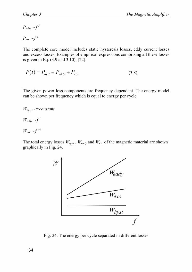
Whyst ~ =constant
Weddy ~ f 1
Wexc ~ f n-1
The total energy losses Whyst , Weddy and Wexc of the magnetic material are shown graphically in Fig. 24.
Fig. 24. The energy per cycle separated in different losses
exceddyhyst PPPtP ++=)(
The Magnetic Amplifier Chapter 3
35
The previous given expression for the total losses can be compared with the empirical equations for the total iron losses given by Metglas for the alloy 2714A [19]:
7.157.161093.9 BfP ⋅⋅⋅= − (3.9)
For the material 2605TCA core losses is graphically given in Fig. 22 by the manufacturer. The Eq. (3.10) is extracted from these graphs.
7.157.161088 BfP ⋅⋅⋅= − (3.10)
,which gives good compliance with the given data in Fig. 22 up to 10 000 Hz. These losses also are showed to be approximately 9 times bigger than those given by Eq. (3.9).

Magnetic Amplifier Demonstrators Chapter 4
37
Chapter 4
Magnetic Amplifier Demonstrators
4.1 The Magnetic Amplifier Demonstrator
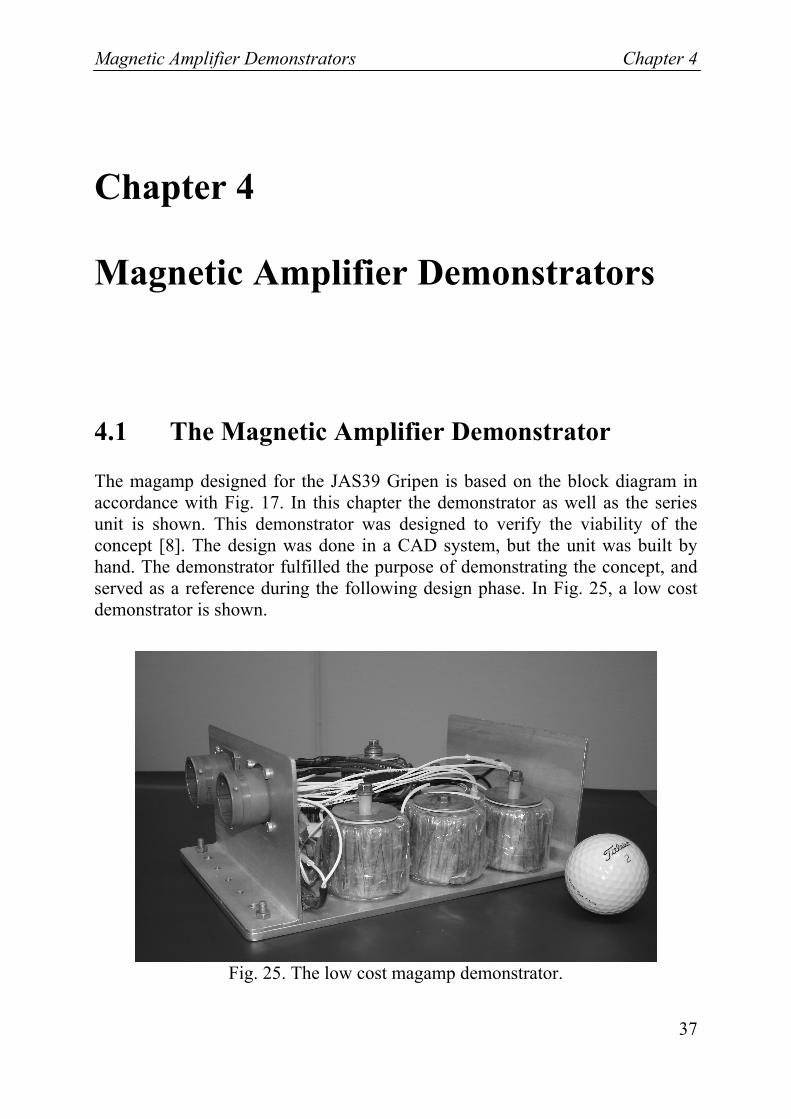
The magamp designed for the JAS39 Gripen is based on the block diagram in accordance with Fig. 17. In this chapter the demonstrator as well as the series unit is shown. This demonstrator was designed to verify the viability of the concept [8]. The design was done in a CAD system, but the unit was built by hand. The demonstrator fulfilled the purpose of demonstrating the concept, and served as a reference during the following design phase. In Fig. 25, a low cost demonstrator is shown.
Fig. 25. The low cost magamp demonstrator.
Chapter 4 Magnetic Amplifier Demonstrators
38
4.2 The JAS39 Gripen Magamp
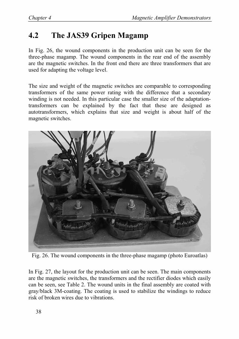
In Fig. 26, the wound components in the production unit can be seen for the three-phase magamp. The wound components in the rear end of the assembly are the magnetic switches. In the front end there are three transformers that are used for adapting the voltage level.
The size and weight of the magnetic switches are comparable to corresponding transformers of the same power rating with the difference that a secondary winding is not needed. In this particular case the smaller size of the adaptation- transformers can be explained by the fact that these are designed as autotransformers, which explains that size and weight is about half of the magnetic switches.
Fig. 26. The wound components in the three-phase magamp (photo Euroatlas)
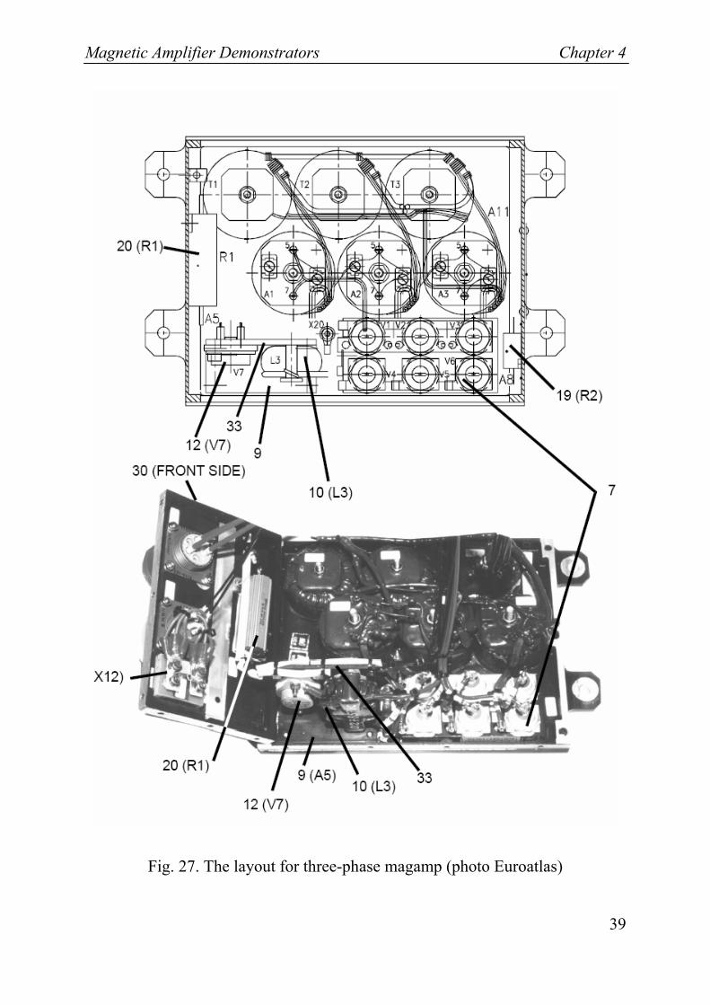
In Fig. 27, the layout for the production unit can be seen. The main components are the magnetic switches, the transformers and the rectifier diodes which easily can be seen, see Table 2. The wound units in the final assembly are coated with gray/black 3M-coating. The coating is used to stabilize the windings to reduce risk of broken wires due to vibrations.
Magnetic Amplifier Demonstrators Chapter 4
39
Fig. 27. The layout for three-phase magamp (photo Euroatlas)
Chapter 4 Magnetic Amplifier Demonstrators
40
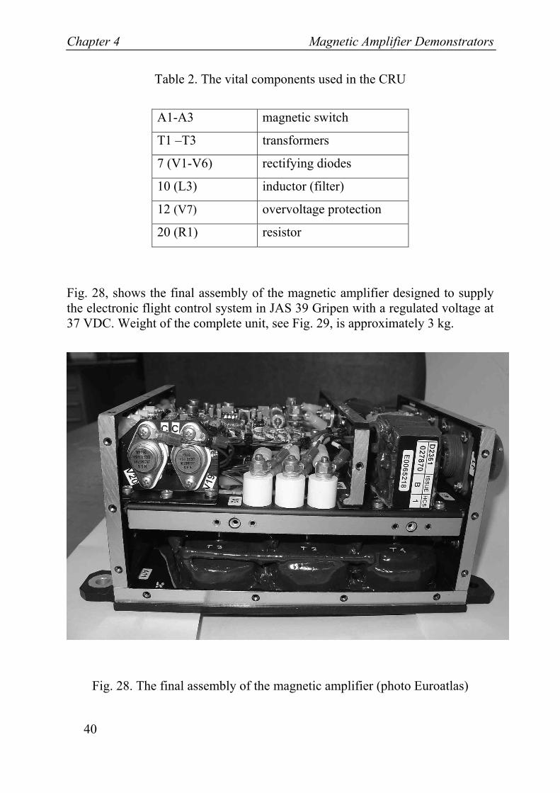
Table 2. The vital components used in the CRU
A1-A3 magnetic switch
T1 –T3 transformers
7 (V1-V6) rectifying diodes
10 (L3) inductor (filter)
12 (V7) overvoltage protection
20 (R1) resistor
Fig. 28, shows the final assembly of the magnetic amplifier designed to supply the electronic flight control system in JAS 39 Gripen with a regulated voltage at 37 VDC. Weight of the complete unit, see Fig. 29, is approximately 3 kg.
Fig. 28. The final assembly of the magnetic amplifier (photo Euroatlas)
Magnetic Amplifier Demonstrators Chapter 4
41
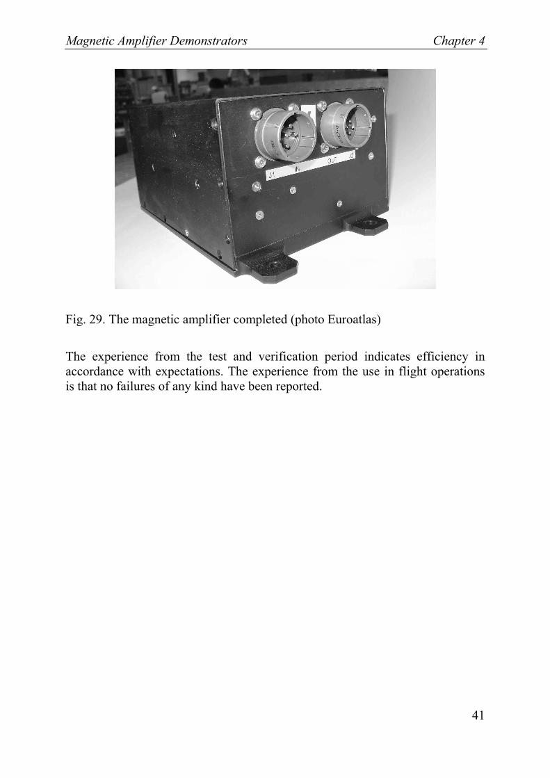
Fig. 29. The magnetic amplifier completed (photo Euroatlas)
The experience from the test and verification period indicates efficiency in accordance with expectations. The experience from the use in flight operations is that no failures of any kind have been reported.

Magnetic Amplifier Models Chapter 5
43
Chapter 5
Magnetic Amplifier Models
5.1 Equivalent Circuit of the Magnetic Switch
In the process of analyzing a magnetic core during operation models for the magnetic properties such as model for hysteresis can be used. Simplified relations [5] constitute useful tools in the concept phase of a design that later is complemented with more detailed simulation models.
A circuit model is shown in Fig. 31. This model can be used to simulate the behaviour of a magnetic switch in a magamp circuit including static effects and stationary losses.
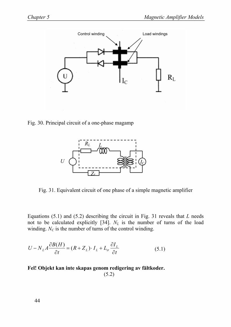
The basic functional arrangement of a magnetic amplifier comprises a magnetic core, usually in form of a two toroids with two load and one control winding, see Fig. 30.
Without current IC in the control winding, the inductance of the load windings, is high, implying a switched-off condition. When IC magnetically saturates the core, the load winding inductance will be low, implying a switched-on load condition.
Chapter 5 Magnetic Amplifier Models
44
Fig. 30. Principal circuit of a one-phase magamp
Fig. 31. Equivalent circuit of one phase of a simple magnetic amplifier
Equations (5.1) and (5.2) describing the circuit in Fig. 31 reveals that L needs not to be calculated explicitly [34]. NL is the number of turns of the load winding. NC is the number of turns of the control winding.
tILIZR
tHBANU L
LLL ∂∂
+⋅+=∂
∂− σ)()(
(5.1)
Fel! Objekt kan inte skapas genom redigering av fältkoder. (5.2)
Load windings Control winding
L
ZL
IC
RL
U
Magnetic Amplifier Models Chapter 5
45
5.2 The Core Model
5.2.1 The Static Hysteresis Model The Bergqvist model is based on that a magnetic material consists of a finite number np of pseudo particles, i.e. volume fractions with different magnetization
With no hysteresis present the magnetization would follow an anhysteretic curve, Man. The hysteresis is introduced by using play operators for each volume fraction with plays equal to their pinning strengths.
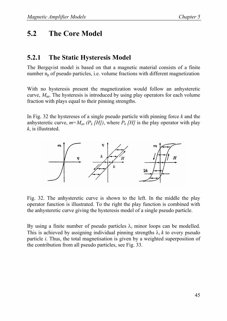
In Fig. 32 the hystereses of a single pseudo particle with pinning force k and the anhysteretic curve, m=Man (Pk [H]), where Pk [H] is the play operator with play k, is illustrated.
Fig. 32. The anhysteretic curve is shown to the left. In the middle the play operator function is illustrated. To the right the play function is combined with the anhysteretic curve giving the hysteresis model of a single pseudo particle.
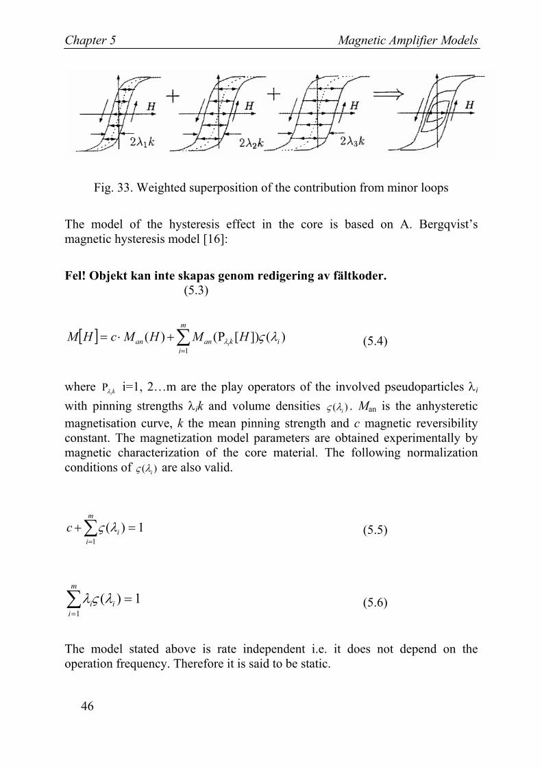
By using a finite number of pseudo particles λi minor loops can be modelled. This is achieved by assigning individual pinning strengths λi k to every pseudo particle i. Thus, the total magnetisation is given by a weighted superposition of the contribution from all pseudo particles, see Fig. 33.
Chapter 5 Magnetic Amplifier Models
46
Fig. 33. Weighted superposition of the contribution from minor loops
The model of the hysteresis effect in the core is based on A. Bergqvist’s magnetic hysteresis model [16]:
Fel! Objekt kan inte skapas genom redigering av fältkoder. (5.3)
[ ] ∑=
Ρ+⋅=m
iikanan HMHMcHM
i1
)(])[()( λςλ (5.4)
where kiλΡ i=1, 2…m are the play operators of the involved pseudoparticles λi
with pinning strengths λik and volume densities ( )iς λ . Man is the anhysteretic magnetisation curve, k the mean pinning strength and c magnetic reversibility constant. The magnetization model parameters are obtained experimentally by magnetic characterization of the core material. The following normalization conditions of ( )iς λ are also valid.
1)(1
=+∑=
m
iic λς (5.5)
1)(1
=∑=
m
iii λςλ (5.6)
The model stated above is rate independent i.e. it does not depend on the operation frequency. Therefore it is said to be static.
Magnetic Amplifier Models Chapter 5
47
5.2.2 Eddy current and excess loss phenomena The complete core model includes static hysteresis losses, eddy current losses and excess losses. An overall expression comprising all these losses is given in Eq (5.7) and (5.8) [22].
(5.7)
(5.8)
The second term can be derived from Faraday’s induction and represents the induced eddy currents. The last is suggested be G. Bertotti [22] and represents the excess losses.
The losses expressed in Eq. (5.8) correspond to the MMF drops according to Eqs. (5.9) and (5.10).
(5.9)
⎟⎠⎞
⎜⎝⎛
⎟⎟⎠
⎞⎜⎜⎝
⎛−+=
dtdBsign
dtdB
VnGdwVnHexc 141
2 02
0
00 σ (5.10)
⎟⎠⎞
⎜⎝⎛⎟⎟⎠
⎞⎜⎜⎝
⎛−++⎟
⎠⎞
⎜⎝⎛+=
dtdB
dtdB
VnGdwVn
dtdBdtPtP hyst 141
212)()(
02
0
0022 σσ
exceddyhyst PPPtP ++=)(
⎟⎠⎞
⎜⎝⎛=
dtdBdHeddy 12
2σ
Chapter 5 Magnetic Amplifier Models
48
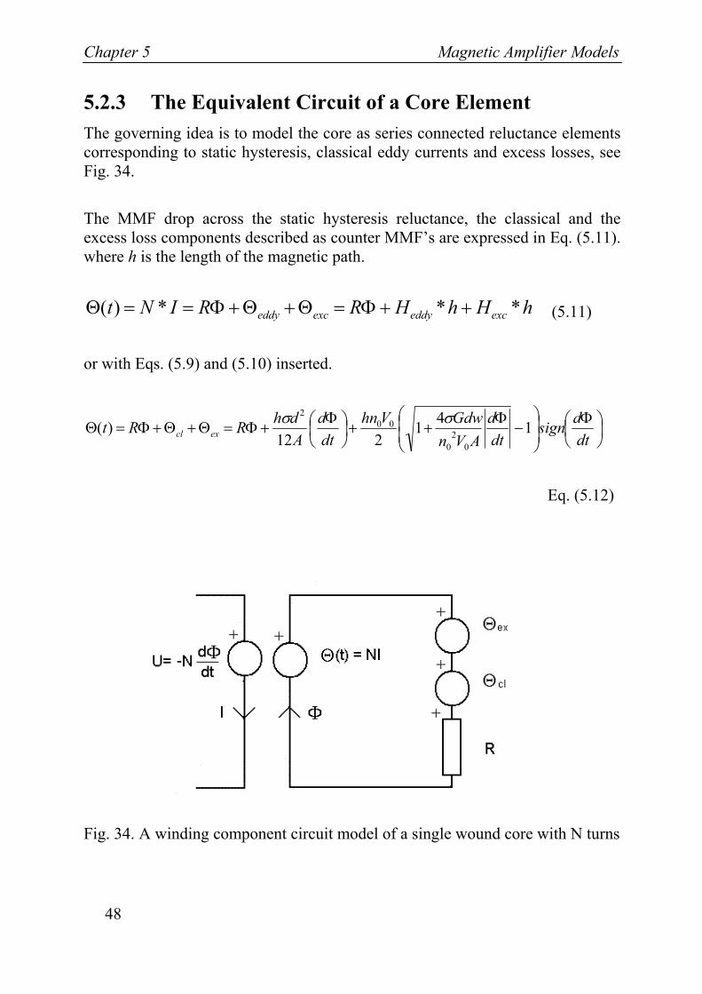
5.2.3 The Equivalent Circuit of a Core Element The governing idea is to model the core as series connected reluctance elements corresponding to static hysteresis, classical eddy currents and excess losses, see Fig. 34.
The MMF drop across the static hysteresis reluctance, the classical and the excess loss components described as counter MMF’s are expressed in Eq. (5.11). where h is the length of the magnetic path.
hHhHRRINt exceddyexceddy ***)( ++Φ=Θ+Θ+Φ==Θ (5.11)
or with Eqs. (5.9) and (5.10) inserted.
⎟⎠⎞
⎜⎝⎛ Φ
⎟⎟⎠
⎞⎜⎜⎝
⎛−
Φ++⎟
⎠⎞
⎜⎝⎛ Φ
+Φ=Θ+Θ+Φ=Θdtdsign
dtd
AVnGdwVhn
dtd
AdhRRt excl 141
212)(
02
0
002 σσ
Eq. (5.12)
Fig. 34. A winding component circuit model of a single wound core with N turns
Magnetic Amplifier Models Chapter 5
49
The first term of (5.10) originates from the static hysteresis model of A. Bergqvist [16]. The second term of originates from the classical eddy current model and the last term representing the excess losses from G. Bertotti [22].
)(tΘ represents the total resulting MMF drop in the core.
The parameters h and A are the bulk length and cross sectional area of the core respectively, σ the electrical conductivity of the core material and d the ribbon thickness. G is a parameter depending on the structure of the magnetic domains, no is a phenomenological parameter related to the number of active correlation regions when f →0, whereas V0 determines how much micro structural features affect the number of correlated regions, w is the width of the ribbon [16].
The parameters no and V0 can be determined indirectly by measurements of the core losses at different frequencies. The pure reluctance element represents the static hysteresis and is managed by the earlier presented hysteresis model [16]. The second term represents the occurring eddy currents in the ribbon of thickness d.
5.3 Simulation Examples
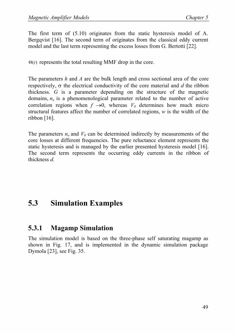
5.3.1 Magamp Simulation The simulation model is based on the three-phase self saturating magamp as shown in Fig. 17, and is implemented in the dynamic simulation package Dymola [23], see Fig. 35.
Chapter 5 Magnetic Amplifier Models
50
Fig. 35. Magamp simulation model
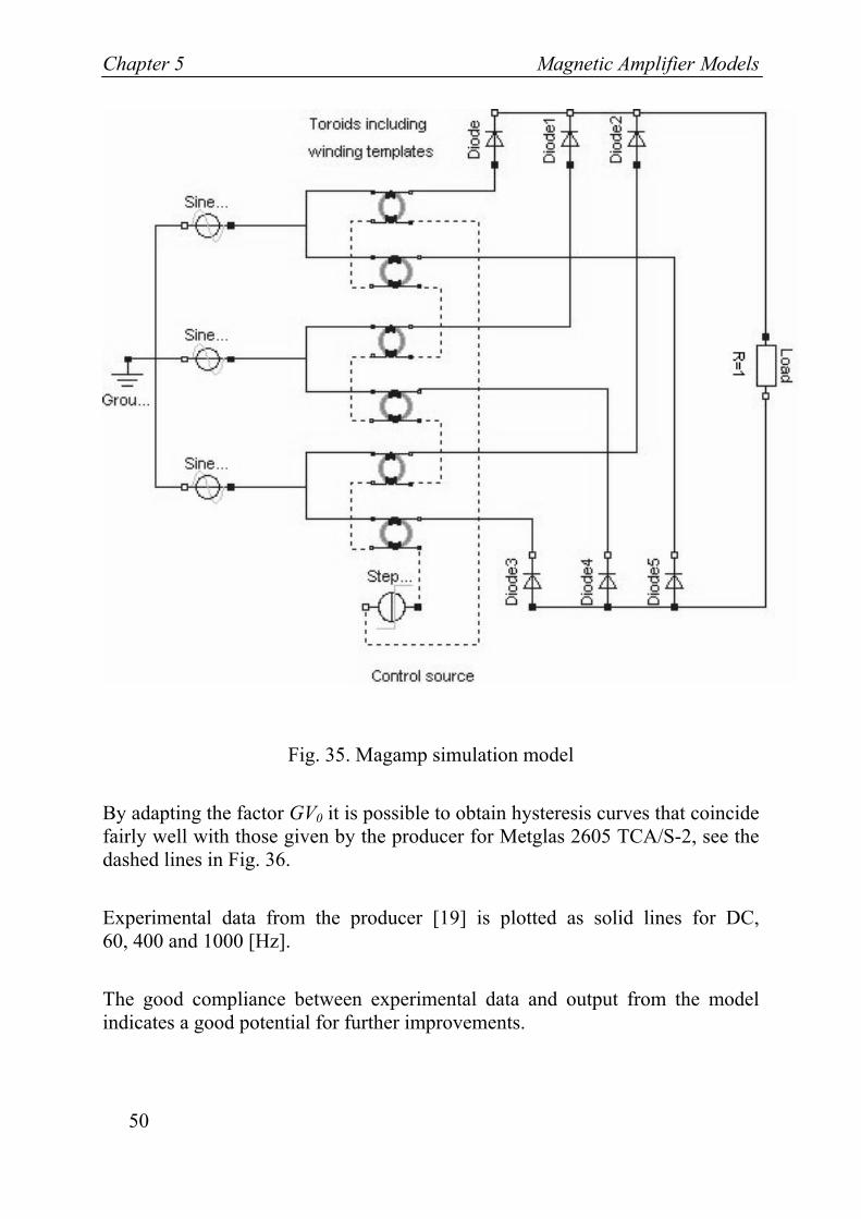
By adapting the factor GV0 it is possible to obtain hysteresis curves that coincide fairly well with those given by the producer for Metglas 2605 TCA/S-2, see the dashed lines in Fig. 36.
Experimental data from the producer [19] is plotted as solid lines for DC, 60, 400 and 1000 [Hz].
The good compliance between experimental data and output from the model indicates a good potential for further improvements.
Magnetic Amplifier Models Chapter 5
51
Fig. 36. Hysteresis model for Metglas 2605 TCA/S-2 Characteristics for different frequencies. The solid lines are the producers data, the dashed lines are major loops generated by the model.
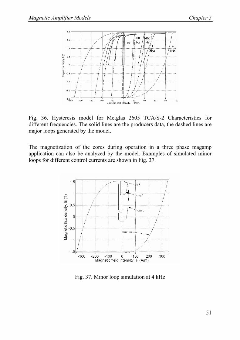
The magnetization of the cores during operation in a three phase magamp application can also be analyzed by the model. Examples of simulated minor loops for different control currents are shown in Fig. 37.
Fig. 37. Minor loop simulation at 4 kHz
Chapter 5 Magnetic Amplifier Models
52
Note that the major loop for 4 kHz, in Fig. 36 differs from that in Fig. 37. This is due to more rapid variations in the flux, corresponding to a higher magnetization field occurring in the application simulated and shown in Fig. 37.
5.3.1.1 The Magamp Losses In the work presented in the thesis the efforts are concentrated on modeling of the core losses (the static hysteresis, the classical and the excess loss components), and the related copper losses in the power windings. The magamp as presented in Fig. 17 contains diodes and a control winding that also generates losses. Since the configuration of the magamp can differ, diode losses and copper losses in the control winding are not considered in this work.
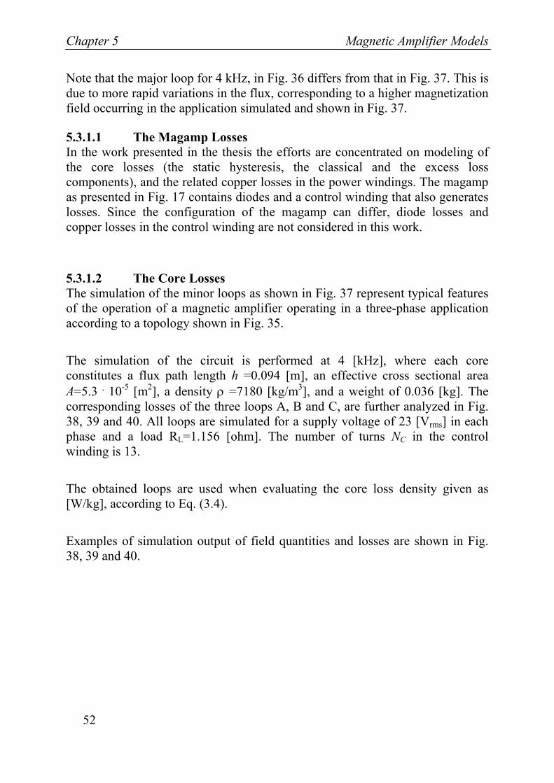
5.3.1.2 The Core Losses The simulation of the minor loops as shown in Fig. 37 represent typical features of the operation of a magnetic amplifier operating in a three-phase application according to a topology shown in Fig. 35.
The simulation of the circuit is performed at 4 [kHz], where each core constitutes a flux path length h =0.094 [m], an effective cross sectional area A=5.3 • 10-5 [m2], a density ρ =7180 [kg/m3], and a weight of 0.036 [kg]. The corresponding losses of the three loops A, B and C, are further analyzed in Fig. 38, 39 and 40. All loops are simulated for a supply voltage of 23 [Vrms] in each phase and a load RL=1.156 [ohm]. The number of turns NC in the control winding is 13.
The obtained loops are used when evaluating the core loss density given as [W/kg], according to Eq. (3.4).
Examples of simulation output of field quantities and losses are shown in Fig. 38, 39 and 40.
Magnetic Amplifier Models Chapter 5
53
Fig. 38. Simulated field quantities and losses as functions of time for loop A
In loop A with IC=0 [A], the magamp operates at a power output of 1200 [W]. The corresponding core loss density then is 0.73 [W/kg] giving PAcore= 0.026 [W]. Note the high H-field due to saturation of the core, during the conducting phase of the magamp.
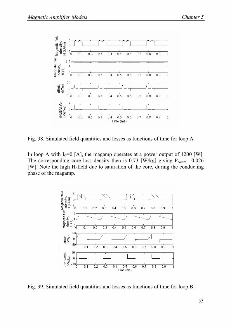
Fig. 39. Simulated field quantities and losses as functions of time for loop B
Chapter 5 Magnetic Amplifier Models
54
In loop B with IC=0.1 [A], the magamp operates at a power output of 730 [W]. The corresponding core loss density then is 15.3 [W/kg] giving PBcore= 0.55 [W].
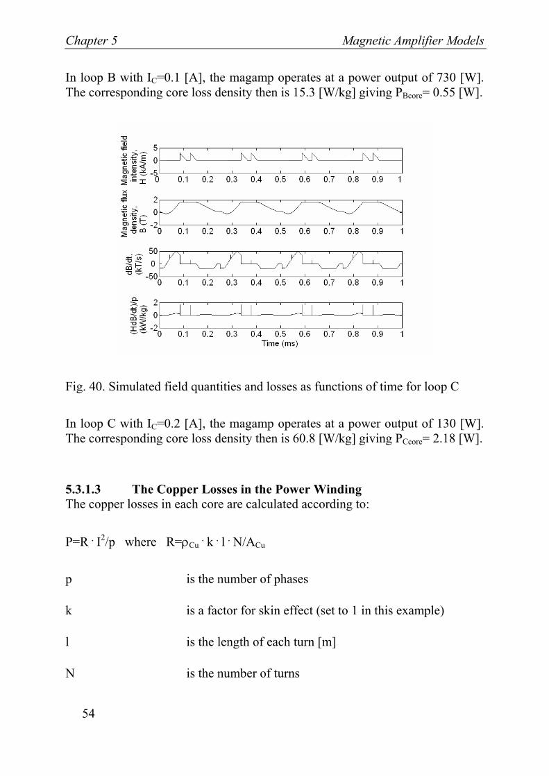
Fig. 40. Simulated field quantities and losses as functions of time for loop C
In loop C with IC=0.2 [A], the magamp operates at a power output of 130 [W]. The corresponding core loss density then is 60.8 [W/kg] giving PCcore= 2.18 [W].
5.3.1.3 The Copper Losses in the Power Winding The copper losses in each core are calculated according to:
P=R • I2/p where R=ρCu • k • l • N/ACu
p is the number of phases
k is a factor for skin effect (set to 1 in this example)
l is the length of each turn [m]
N is the number of turns
Magnetic Amplifier Models Chapter 5
55
ACu is the cross sectional area of the copper wire [m2]
ρCu is the resistivity of 2.15 • 10-8 [ohm ⋅m] when operating at a temperature of 85 [°C].
The copper losses are PACu= 0.73 [W], PBCu= 0.44 and PCCu= 0.08 [W] respectively, given by the simulations where p=3, l=0.047 [m], N=13, ACu =5 • 10-6[m].
5.3.1.4 The Magamp Efficiency In the simulated examples, the magamp in Fig. 38, 39 and 40 is operated at 1200 [W], 730 [W] and 130 [W] for loop A, B and C respectively. The simulations yield the total losses of each core PA=PAcore+PACu = 0.76 [W], PB= 0.99 [W] and PC= 2.26 [W], for loop A, B and C respectively.
The efficiency, defined as the input power minus the losses of six cores divided by the input power, gives an efficiency of 99.6 %, 99.2% and 90.6 % for the magamp operating at loops A, B and C respectively.
5.3.1.5 Detailed Simulation The so far performed simulations are done on the three-phase self saturating magamp shown in Fig. 17, The control current, IC, has been 0, 0.1 and 0.2 A i.e. zero control current or a positive control current taking the core out of saturation.
This detailed simulation will be the reference and compared with tests performed with negative control currents in section 5.4.1.6.
Initially a detailed simulation with zero control current i.e. IC=0 mA is performed, shown in Fig. 41 where details of the minor loop can be studied. The examples shown in Fig. 41, 42 and 43 shall only be compared with each other.
Chapter 5 Magnetic Amplifier Models
56
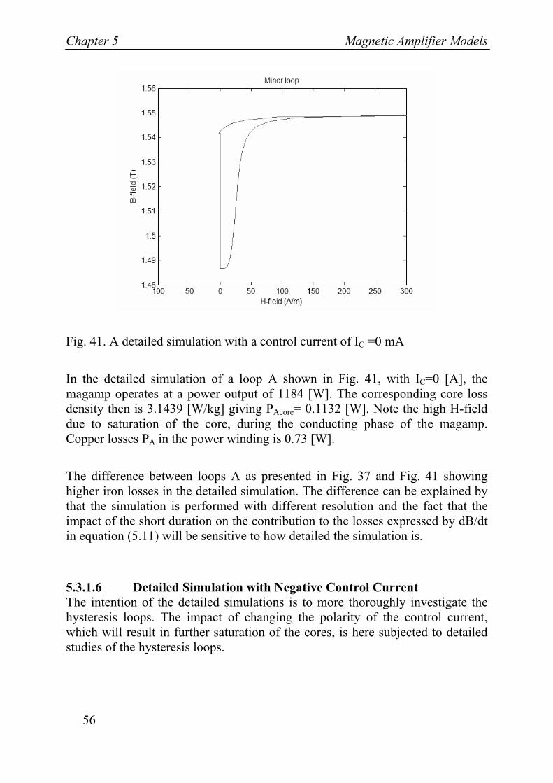
Fig. 41. A detailed simulation with a control current of IC =0 mA
In the detailed simulation of a loop A shown in Fig. 41, with IC=0 [A], the magamp operates at a power output of 1184 [W]. The corresponding core loss density then is 3.1439 [W/kg] giving PAcore= 0.1132 [W]. Note the high H-field due to saturation of the core, during the conducting phase of the magamp. Copper losses PA in the power winding is 0.73 [W].
The difference between loops A as presented in Fig. 37 and Fig. 41 showing higher iron losses in the detailed simulation. The difference can be explained by that the simulation is performed with different resolution and the fact that the impact of the short duration on the contribution to the losses expressed by dB/dt in equation (5.11) will be sensitive to how detailed the simulation is.
5.3.1.6 Detailed Simulation with Negative Control Current The intention of the detailed simulations is to more thoroughly investigate the hysteresis loops. The impact of changing the polarity of the control current, which will result in further saturation of the cores, is here subjected to detailed studies of the hysteresis loops.
Magnetic Amplifier Models Chapter 5
57
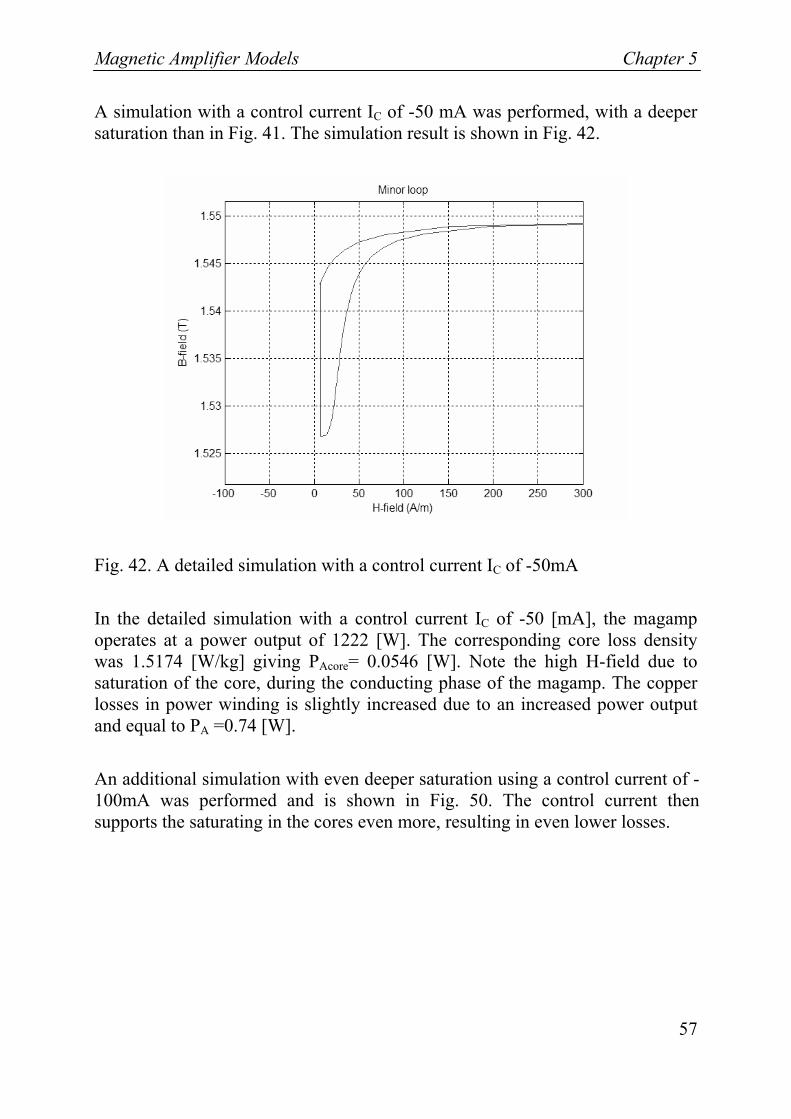
A simulation with a control current IC of -50 mA was performed, with a deeper saturation than in Fig. 41. The simulation result is shown in Fig. 42.
Fig. 42. A detailed simulation with a control current IC of -50mA
In the detailed simulation with a control current IC of -50 [mA], the magamp operates at a power output of 1222 [W]. The corresponding core loss density was 1.5174 [W/kg] giving PAcore= 0.0546 [W]. Note the high H-field due to saturation of the core, during the conducting phase of the magamp. The copper losses in power winding is slightly increased due to an increased power output and equal to PA =0.74 [W].
An additional simulation with even deeper saturation using a control current of -100mA was performed and is shown in Fig. 50. The control current then supports the saturating in the cores even more, resulting in even lower losses.
Chapter 5 Magnetic Amplifier Models
58
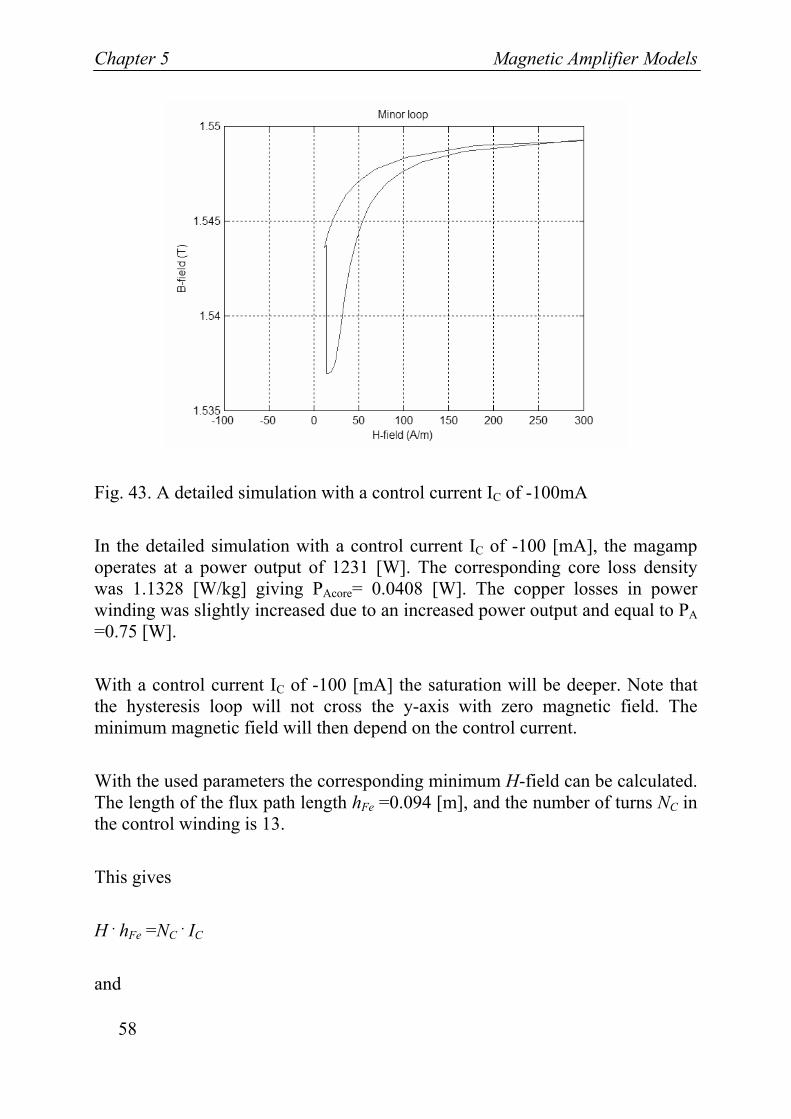
Fig. 43. A detailed simulation with a control current IC of -100mA
In the detailed simulation with a control current IC of -100 [mA], the magamp operates at a power output of 1231 [W]. The corresponding core loss density was 1.1328 [W/kg] giving PAcore= 0.0408 [W]. The copper losses in power winding was slightly increased due to an increased power output and equal to PA =0.75 [W].
With a control current IC of -100 [mA] the saturation will be deeper. Note that the hysteresis loop will not cross the y-axis with zero magnetic field. The minimum magnetic field will then depend on the control current.
With the used parameters the corresponding minimum H-field can be calculated. The length of the flux path length hFe =0.094 [m], and the number of turns NC in the control winding is 13.
This gives
H • hFe =NC • IC
and
Magnetic Amplifier Models Chapter 5
59
H=13 • 0.1/0.094= 13.8 [A/m],
which is a result that complies with the simulation shown in Fig 43.
The examples in Fig. 42 and 43 indicate that saturation control can further improve the efficiency, with reduced core losses, as well as increased output power of the magamp. With a control current that saturates the core the magnetic field remains positive during the complete hysteresis loop. The examples shown in Fig. 41, 42 and 43 shall only be compared with each other.
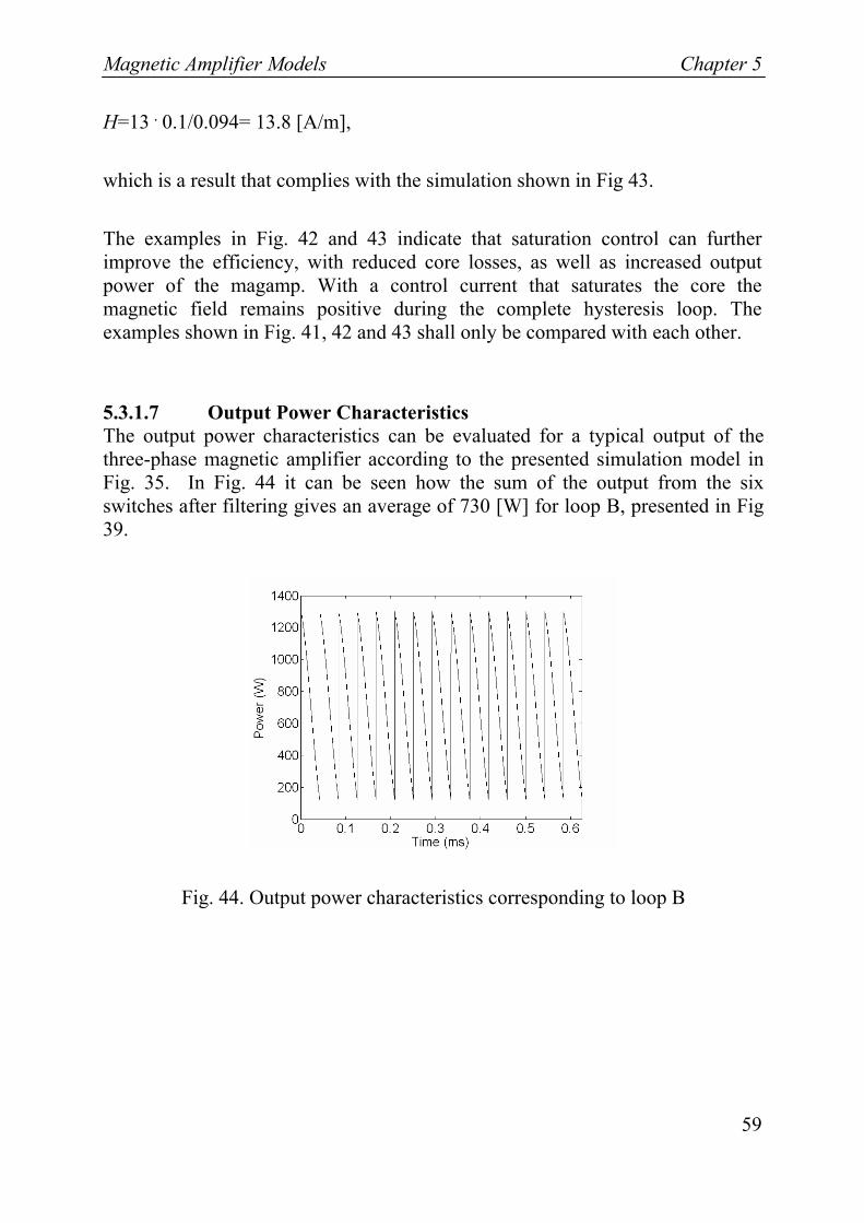
5.3.1.7 Output Power Characteristics The output power characteristics can be evaluated for a typical output of the three-phase magnetic amplifier according to the presented simulation model in Fig. 35. In Fig. 44 it can be seen how the sum of the output from the six switches after filtering gives an average of 730 [W] for loop B, presented in Fig 39.
Fig. 44. Output power characteristics corresponding to loop B
Chapter 5 Magnetic Amplifier Models
60
5.4 Analysis of Losses and Weight of a Magamp Core
The iron losses per kilo can be described as a function of frequency and peak flux density, $B . In evaluation of the iron losses in a magamp application, with unsymmetrical flux, the peak flux density is half of the peak to peak value of the flux.
Eq. (5.13) constitutes such an empirical function is given by Metglas [19] for the amorphous material 2714A.
7.157.161093.9 BfP ⋅⋅⋅= − (5.13)
For the material 2605TCA the core losses are graphically given in Fig. 22 by the manufacturer. The Eq. (5.14) is extracted, based on these graphs.
7.157.161088 BfP ⋅⋅⋅= − (5.14)
,which yields good compliance with data in Fig. 22 up to 10 000 Hz. These losses also are showed to be approximately 9 times bigger than those obtained from equation (5.13).
The weight of the core is:
ρ⋅⋅= FeFe Ahm (5.15)
where hFe is the average iron flux path length, AFe the average core cross sectional area and ρ is the density of the different alloys:
2714A ρ=7590 kg/m3
2605TCA ρ=7180 kg/m3
Magnetic Amplifier Models Chapter 5
61
The relation between number of turns, N, and the average core cross sectional area, AFe, is given in equation (5.16). The parameters such as peak flux density $B , voltage, E, and frequency are given by the operational requirements.
Fel! Objekt kan inte skapas genom redigering av fältkoder. (5.16)
Note for square wave applications the factor 4.44 is changed to 4.00.
The frequency can be described in terms of the period time T. The voltage-time product TU ⋅ is calculated.
NABTU Fe ⋅⋅⋅=⋅ 2 (5.17)
The flux density span is 2B, because the flux can be used over the whole span from negative to positive B.
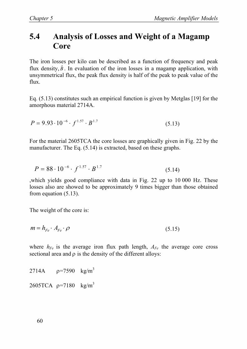
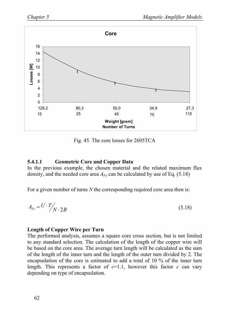
5.4.1 Graphical Analysis Example In Fig. 45 a graphical example is given for a three phase magamp, designed for an output power of 10 000 W, with an output voltage of 270 VDC. The core losses are estimated by equation (5.14), and the weight by equation (5.15).
The graph is based on different number of turns, N. The resulting core losses are calculated for different core cross sectional areas, AFe, see Eq. (5.17). The corresponding core weights are shown in the figure.
Chapter 5 Magnetic Amplifier Models
62
Fig. 45. The core losses for 2605TCA
5.4.1.1 Geometric Core and Copper Data In the previous example, the chosen material and the related maximum flux density, and the needed core area AFe can be calculated by use of Eq. (5.18)
For a given number of turns N the corresponding required core area then is:
BNTUAFe 2⋅⋅= (5.18)
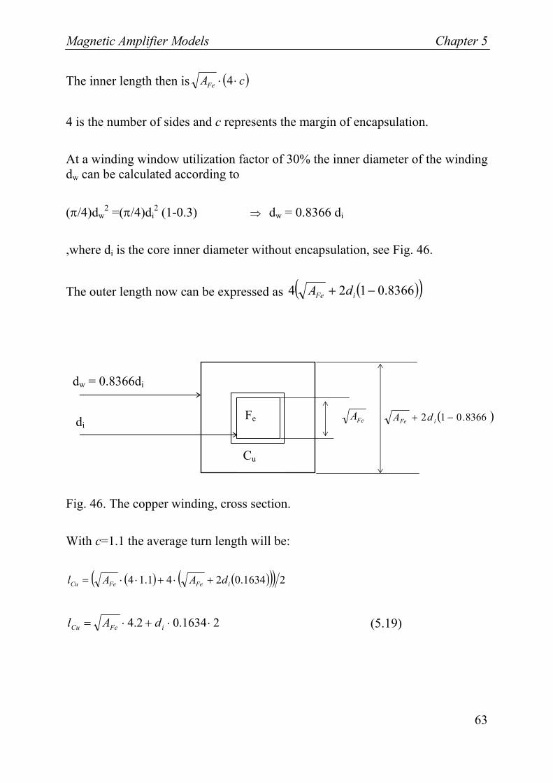
Length of Copper Wire per Turn The performed analysis, assumes a square core cross section, but is not limited to any standard selection. The calculation of the length of the copper wire will be based on the core area. The average turn length will be calculated as the sum of the length of the inner turn and the length of the outer turn divided by 2. The encapsulation of the core is estimated to add a total of 10 % of the inner turn length. This represents a factor of c=1.1, however this factor c can vary depending on type of encapsulation.
Core
0
2
4
6
8
10
12
14
16
129,2 80,3 50,0 34,9 27,3
Weight [gram] Number of Turns
Loss
es [W
]
15 25 45 75 110
l
ll
Magnetic Amplifier Models Chapter 5
63
The inner length then is ( )cAFe ⋅⋅ 4
4 is the number of sides and c represents the margin of encapsulation.
At a winding window utilization factor of 30% the inner diameter of the winding dw can be calculated according to
(π/4)dw2 =(π/4)di
2 (1-0.3) ⇒ dw = 0.8366 di
,where di is the core inner diameter without encapsulation, see Fig. 46.
The outer length now can be expressed as ( )( )8366.0124 −+ iFe dA
Fig. 46. The copper winding, cross section.
With c=1.1 the average turn length will be:
( ) ( )( )( ) 21634.0241.14 iFeFeCu dAAl +⋅+⋅⋅=
21634.02.4 ⋅⋅+⋅= iFeCu dAl (5.19)
FeAFe
Cu
dw = 0.8366di
di ( )8366.012 −+ iFe dA
Chapter 5 Magnetic Amplifier Models
64
5.4.1.2 Copper Losses The copper losses are basically depending on the current, the turn length, number of turns and the copper area ACu. The wire length is calculated by use of the average length per turn, that gives the resistance according to:
CuCu A
NlkR ⋅⋅= ρ , where (5.20)
ρ=2 • 10-8 ohmm at 85 °C
k is the skin factor. At higher frequencies k>1.
For details about the skin factor, see section 6.2.1. It can be noted that there is a very low impact of the skin effect (less than 10%) for a wire of a diameter less than 2 [mm] as long as the frequency is less than 10000 Hz.
The copper losses are: nIRPCu
2⋅= (5.21)
where n is equal to 2, due to the 50 % duty cycle, for a 1 phase magamp and 3 for a 3 phase magamp, and in all other cases n complies with the number of phases.
Weight of Copper Wire The weight of the copper wire is:
ρ⋅⋅⋅= CuANlm (5.22)
where ρ =8900 [kg/m3]
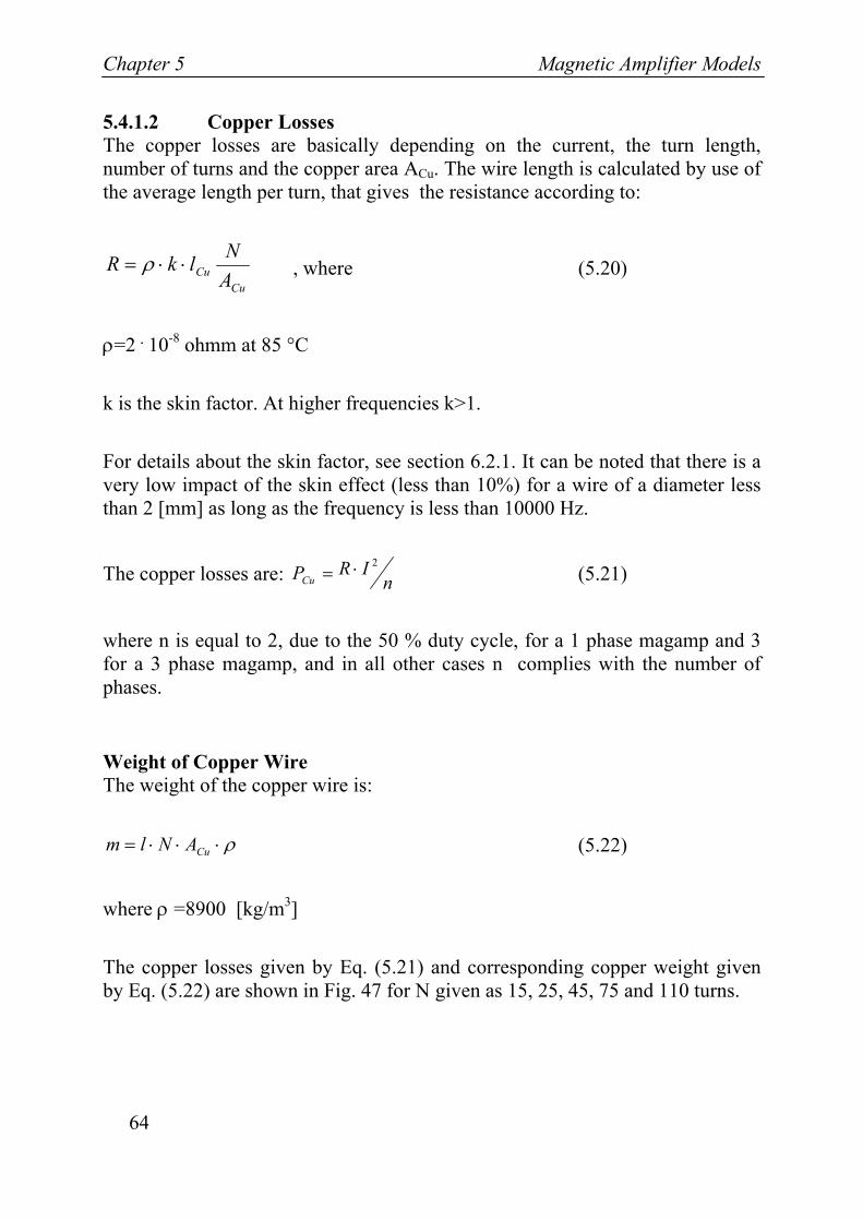
The copper losses given by Eq. (5.21) and corresponding copper weight given by Eq. (5.22) are shown in Fig. 47 for N given as 15, 25, 45, 75 and 110 turns.
Magnetic Amplifier Models Chapter 5
65
Fig. 47. The copper losses
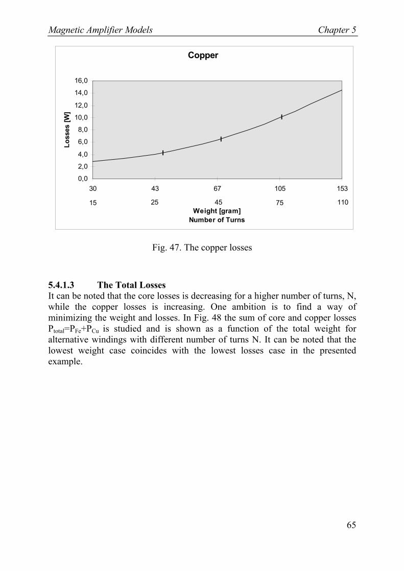
5.4.1.3 The Total Losses It can be noted that the core losses is decreasing for a higher number of turns, N, while the copper losses is increasing. One ambition is to find a way of minimizing the weight and losses. In Fig. 48 the sum of core and copper losses Ptotal=PFe+PCu is studied and is shown as a function of the total weight for alternative windings with different number of turns N. It can be noted that the lowest weight case coincides with the lowest losses case in the presented example.
Copper
0,0
2,0
4,0
6,0
8,0
10,0
12,0
14,0
16,0
30 43 67 105 153
Weight [gram] Number of Turns
Loss
es [W
]
15 25 45 75 110
l
l
l
Chapter 5 Magnetic Amplifier Models
66
Fig. 48. The core and copper losses
5.5 A Proposed Engineering Tool
The proposed engineering tool offers a quick method of analyzing whether a magamp design is possible for a considered application. Weight and efficiency are parameters that are analyzed by the proposed tool. In aircraft design, information regarding e.g. frequency and weight must be communicated between system design [3] and component design groups. This can be accomplished by this engineering tool.
The methodology of analyzing the weight losses in a magamp is demonstrated by:
1. Specify power requirement, output current and voltage
2. Specify number of phases
3. Choose alloy for the cores, and specify max flux density
Core + Copper
02468
101214161820
160 123 117 140 181
Weight [gram] Number of Turns
Loss
es [W
]
15 25 7545
ll
l
110
Magnetic Amplifier Models Chapter 5
67
4. Choose copper area
5. Choose insulation factor
6. Make a preliminary choose of core inner diameter
7. Make a preliminary set up of the number of turns
8. Evaluate graphically given results
The tool automatically calculates iron and copper losses and iron and copper weights given as a function of the given set of turns of the power winding. The winding window utilization factor will automatically be calculated; in this thesis 30 % is used, but can be higher or lower. During the design evaluation in step 8, any of the inputs in step 1-7 can be varied until the magamp meet the design goals, or the best possible compromise is achieved.
The optimization of the magamp can be slightly different depending on the load profile, i.e. whether the magamp is mostly on or off. In an initial study it can be sufficient to look at the sum of the core and copper losses.
Other features as required core size and control current and number of turns are important [33]. As a general rule, the design shall utilize a minimal amount of core material that implies low weight and losses.
Feature The tool estimates output data like weight, dimensions and losses based on defined equations and input data. In similarity with a transistor circuit the magamp must be designed to meet the requirements of current as well as voltage. The difference is that the voltage capability of the magamp is in terms of volts during a period of time [Vs].
Usage Numbers of turns are used as an input parameter. Selections of different number of turns N are used to evaluate weight end losses. The tool gives an opportunity to evaluate weight end losses for different N. It will support the design
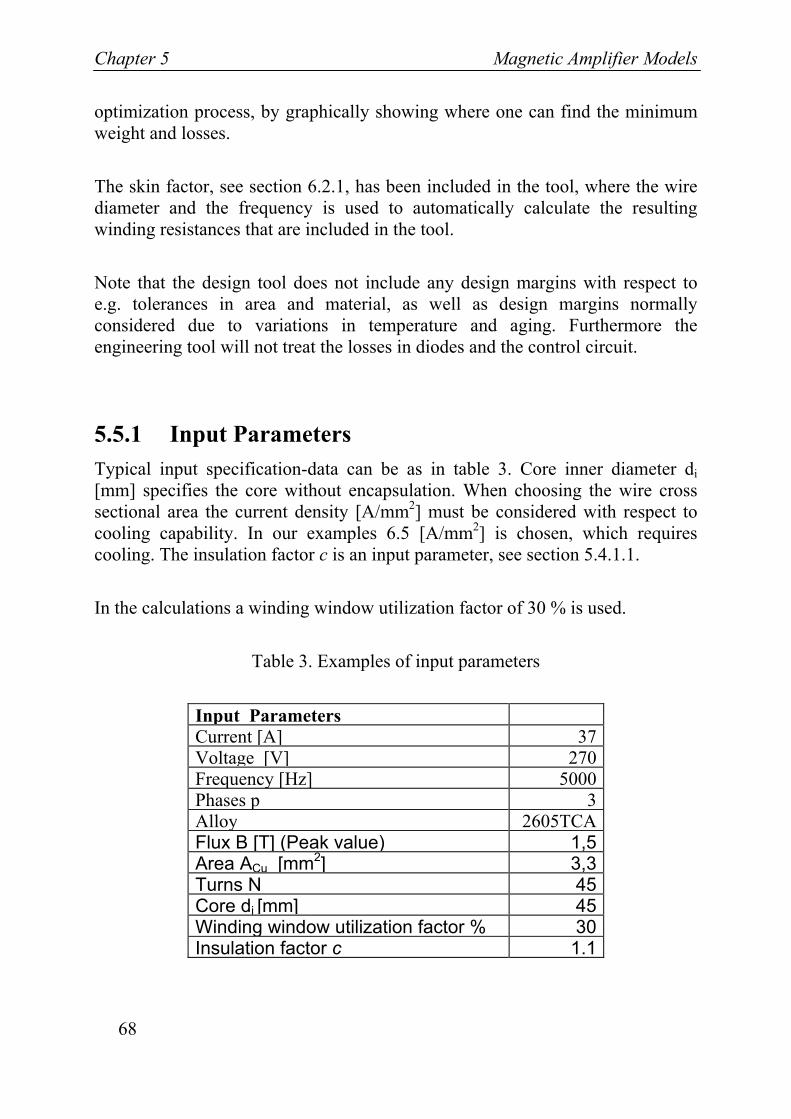
Chapter 5 Magnetic Amplifier Models
68
optimization process, by graphically showing where one can find the minimum weight and losses.
The skin factor, see section 6.2.1, has been included in the tool, where the wire diameter and the frequency is used to automatically calculate the resulting winding resistances that are included in the tool.
Note that the design tool does not include any design margins with respect to e.g. tolerances in area and material, as well as design margins normally considered due to variations in temperature and aging. Furthermore the engineering tool will not treat the losses in diodes and the control circuit.
5.5.1 Input Parameters Typical input specification-data can be as in table 3. Core inner diameter di [mm] specifies the core without encapsulation. When choosing the wire cross sectional area the current density [A/mm2] must be considered with respect to cooling capability. In our examples 6.5 [A/mm2] is chosen, which requires cooling. The insulation factor c is an input parameter, see section 5.4.1.1.
In the calculations a winding window utilization factor of 30 % is used.
Table 3. Examples of input parameters
Input ParametersCurrent [A] 37 Voltage [V] 270 Frequency [Hz] 5000 Phases p 3 Alloy 2605TCA Flux B [T] (Peak value) 1,5 Area ACu [mm2] 3,3 Turns N 45 Core di [mm] 45 Winding window utilization factor % 30 Insulation factor c 1.1
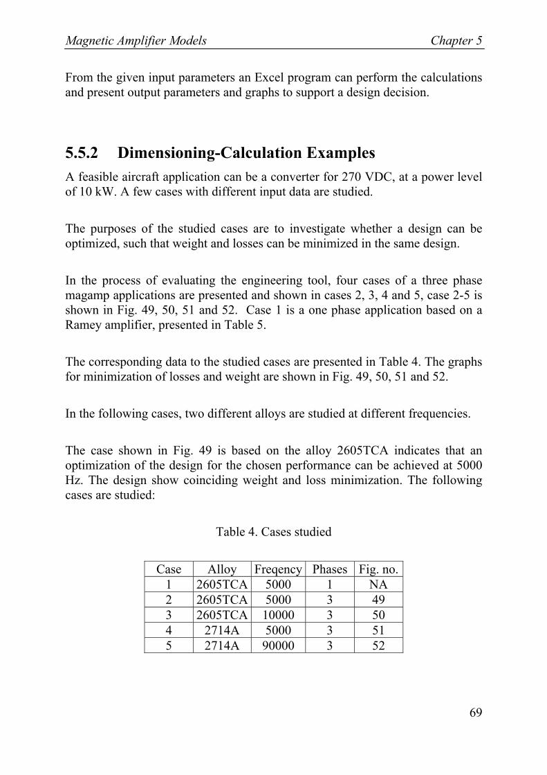
Magnetic Amplifier Models Chapter 5
69
From the given input parameters an Excel program can perform the calculations and present output parameters and graphs to support a design decision.
5.5.2 Dimensioning-Calculation Examples A feasible aircraft application can be a converter for 270 VDC, at a power level of 10 kW. A few cases with different input data are studied.
The purposes of the studied cases are to investigate whether a design can be optimized, such that weight and losses can be minimized in the same design.
In the process of evaluating the engineering tool, four cases of a three phase magamp applications are presented and shown in cases 2, 3, 4 and 5, case 2-5 is shown in Fig. 49, 50, 51 and 52. Case 1 is a one phase application based on a Ramey amplifier, presented in Table 5.
The corresponding data to the studied cases are presented in Table 4. The graphs for minimization of losses and weight are shown in Fig. 49, 50, 51 and 52.
In the following cases, two different alloys are studied at different frequencies.
The case shown in Fig. 49 is based on the alloy 2605TCA indicates that an optimization of the design for the chosen performance can be achieved at 5000 Hz. The design show coinciding weight and loss minimization. The following cases are studied:
Table 4. Cases studied
Case Alloy Freqency Phases Fig. no. 1 2605TCA 5000 1 NA 2 2605TCA 5000 3 49 3 2605TCA 10000 3 50 4 2714A 5000 3 51 5 2714A 90000 3 52
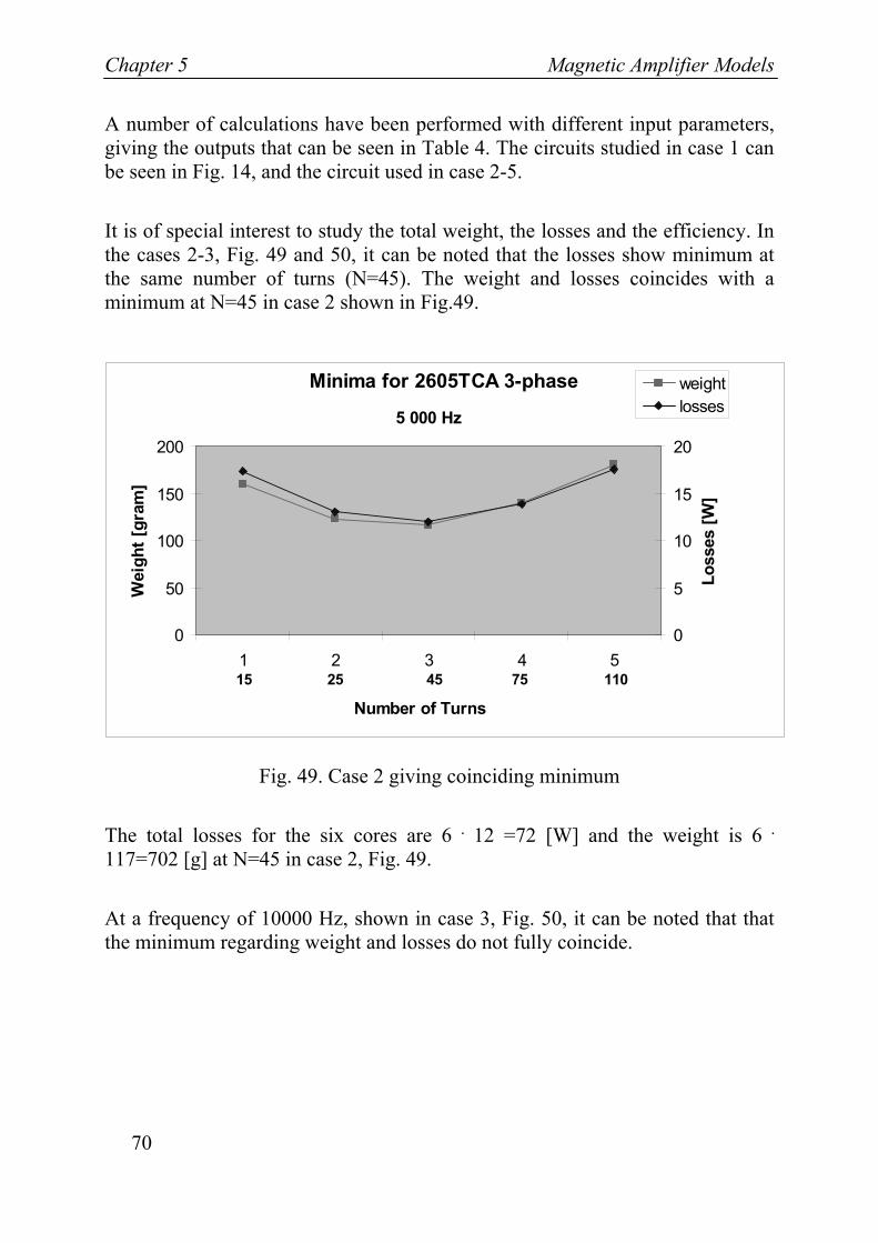
Chapter 5 Magnetic Amplifier Models
70
A number of calculations have been performed with different input parameters, giving the outputs that can be seen in Table 4. The circuits studied in case 1 can be seen in Fig. 14, and the circuit used in case 2-5.
It is of special interest to study the total weight, the losses and the efficiency. In the cases 2-3, Fig. 49 and 50, it can be noted that the losses show minimum at the same number of turns (N=45). The weight and losses coincides with a minimum at N=45 in case 2 shown in Fig.49.
Fig. 49. Case 2 giving coinciding minimum
The total losses for the six cores are 6 • 12 =72 [W] and the weight is 6 • 117=702 [g] at N=45 in case 2, Fig. 49.
At a frequency of 10000 Hz, shown in case 3, Fig. 50, it can be noted that that the minimum regarding weight and losses do not fully coincide.
Minima for 2605TCA 3-phase
0
50
100
150
200
1 2 3 4 5
Number of Turns
Wei
ght [
gram
]
0
5
10
15
20
5 000 Hz
Loss
es [W
]
weightlosses
45 25 75 110 15
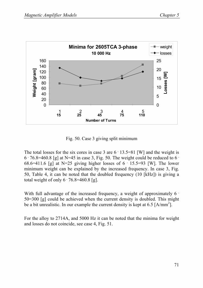
Magnetic Amplifier Models Chapter 5
71
Fig. 50. Case 3 giving split minimum
The total losses for the six cores in case 3 are 6 • 13.5=81 [W] and the weight is 6 • 76.8=460.8 [g] at N=45 in case 3, Fig. 50. The weight could be reduced to 6 • 68.6=411.6 [g] at N=25 giving higher losses of 6 • 15.5=93 [W]. The lower minimum weight can be explained by the increased frequency. In case 3, Fig. 50, Table 4, it can be noted that the doubled frequency (10 [kHz]) is giving a total weight of only 6 • 76.8=460.8 [g].
With full advantage of the increased frequency, a weight of approximately 6 •
50=300 [g] could be achieved when the current density is doubled. This might be a bit unrealistic. In our example the current density is kept at 6.5 [A/mm2].
For the alloy to 2714A, and 5000 Hz it can be noted that the minima for weight and losses do not coincide, see case 4, Fig. 51.
Minima for 2605TCA 3-phase
020406080
100120140160
1 2 3 4 5
Wei
ght [
gram
]
0
5
10
15
20
25
10 000 Hz
Loss
es [W
]
weightlosses
Number of Turns110 15 25 45 75
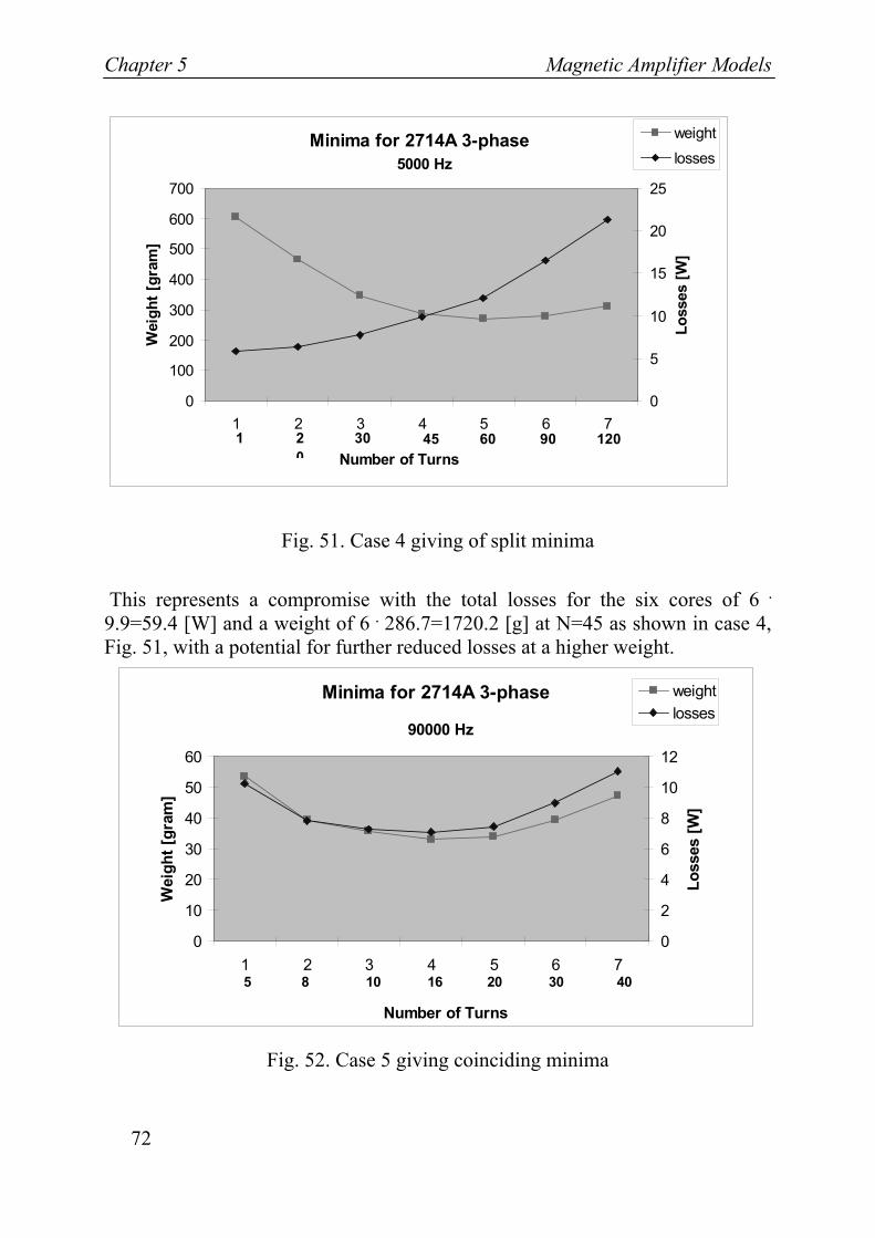
Chapter 5 Magnetic Amplifier Models
72
Minima for 2714A 3-phase
0
100
200
300
400
500
600
700
1 2 3 4 5 6 7
Wei
ght [
gram
]
0
5
10
15
20
255000 Hz
Loss
es [W
]
weightlosses
Number of Turns30 1 2
060 90 120 45
Fig. 51. Case 4 giving of split minima
This represents a compromise with the total losses for the six cores of 6 • 9.9=59.4 [W] and a weight of 6 • 286.7=1720.2 [g] at N=45 as shown in case 4, Fig. 51, with a potential for further reduced losses at a higher weight.
Fig. 52. Case 5 giving coinciding minima
Minima for 2714A 3-phase
0
10
20
30
40
50
60
1 2 3 4 5 6 7
Number of Turns
Wei
ght [
gram
]
0
2
4
6
8
10
12
90000 Hz
Loss
es [W
]weightlosses
5 8 10 16 20 30 40
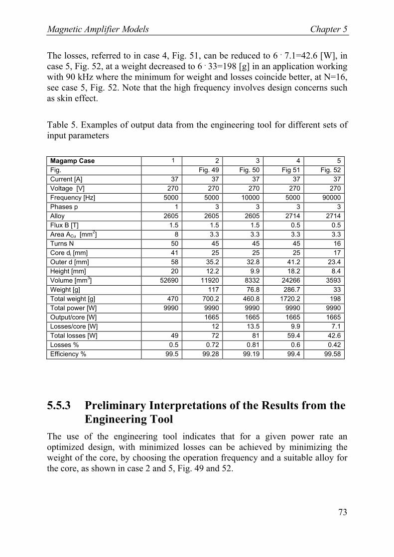
Magnetic Amplifier Models Chapter 5
73
The losses, referred to in case 4, Fig. 51, can be reduced to 6 • 7.1=42.6 [W], in case 5, Fig. 52, at a weight decreased to 6 • 33=198 [g] in an application working with 90 kHz where the minimum for weight and losses coincide better, at N=16, see case 5, Fig. 52. Note that the high frequency involves design concerns such as skin effect.
Table 5. Examples of output data from the engineering tool for different sets of input parameters
Magamp Case 1 2 3 4 5Fig. Fig. 49 Fig. 50 Fig 51 Fig. 52Current [A] 37 37 37 37 37Voltage [V] 270 270 270 270 270Frequency [Hz] 5000 5000 10000 5000 90000Phases p 1 3 3 3 3Alloy 2605 2605 2605 2714 2714Flux B [T] 1.5 1.5 1.5 0.5 0.5Area ACu [mm2] 8 3.3 3.3 3.3 3.3Turns N 50 45 45 45 16Core di [mm] 41 25 25 25 17Outer d [mm] 58 35.2 32.8 41.2 23.4Height [mm] 20 12.2 9.9 18.2 8.4Volume [mm3] 52690 11920 8332 24266 3593Weight [g] 117 76.8 286.7 33Total weight [g] 470 700.2 460.8 1720.2 198Total power [W] 9990 9990 9990 9990 9990Output/core [W] 1665 1665 1665 1665Losses/core [W] 12 13.5 9.9 7.1Total losses [W] 49 72 81 59.4 42.6Losses % 0.5 0.72 0.81 0.6 0.42Efficiency % 99.5 99.28 99.19 99.4 99.58
5.5.3 Preliminary Interpretations of the Results from the Engineering Tool
The use of the engineering tool indicates that for a given power rate an optimized design, with minimized losses can be achieved by minimizing the weight of the core, by choosing the operation frequency and a suitable alloy for the core, as shown in case 2 and 5, Fig. 49 and 52.
Chapter 5 Magnetic Amplifier Models
74
The advantage of a design with the alloy 2605TCA at e.g. 5000 Hz, is that the lowest losses coincide with the lowest weight. The thesis that the iron losses is in proportion to the mass of iron is valid in a magamp application designed to use largest possible flux. The demonstrated optimizations seem to be valid for different cases where the same flux level occurs. The losses can be lowered by using a smaller proportion of the available flux swing, but the consequence then is increased weight. The study indicates that the lowest losses coincide with the lowest weight the losses in the core are about equal to the losses in the copper wire. This can be seen in the cases 2 and 5, shown in Fig. 49 and 52.
It can be noted that the higher the flux density, the lower the weight can be.
This is indicated in case 2, Fig. 49, with an alloy with a max flux density of 1.5 T that yielded a weight of 6 • 117=702 g. In case 4, Fig. 51, with an alloy with a max flux density of 0.5 T the weight was indicated to be 6 • 286.7=1720.2 g.
These examples are identical except for that the used alloys admit different flux densities.
The efficiency of the magnetic amplifiers is estimated to be as high as 99.3 % and the corresponding power-density then easily can meet 14 [kW/kg] in the 5000 [Hz] application.
The conclusion is that a core in the 2605-family is the preferable alloy for audio frequencies, due to the possibility to achieve a design with low weight and thus achieve low losses. The 2714A alloy might be preferable in the 90 kHz range, with a potential of efficiency near 99.6 %. At this frequency the skin effect, however, has increased the resistance that increases the losses, and reduces the efficiency. This problem could be corrected by splitting the current in a number of parallel wires.
5.6 Conclusions
The proposed simulation model approach is considered to be a feasible tool in the design of magnetic amplifiers. This means that the modeling approach can
Magnetic Amplifier Models Chapter 5
75
be used to evaluate magnetic and resistive losses of tentative magnetic amplifier designs.
The engineering tool appears to be a useful tool in the initial stage of a design.
Both the proposed simulation model and the engineering tool need further development. Experimental verifications of the models with electric and/or calorimetric methods remain.

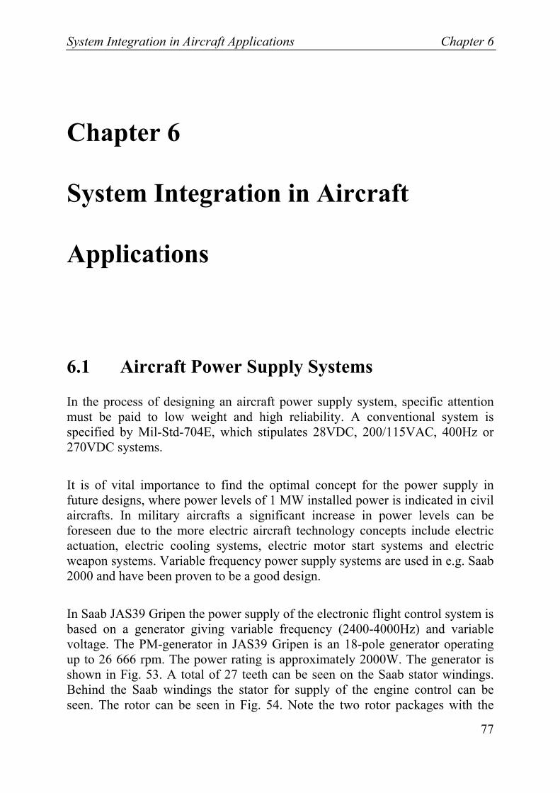
System Integration in Aircraft Applications Chapter 6
77
Chapter 6
System Integration in Aircraft
Applications
6.1 Aircraft Power Supply Systems
In the process of designing an aircraft power supply system, specific attention must be paid to low weight and high reliability. A conventional system is specified by Mil-Std-704E, which stipulates 28VDC, 200/115VAC, 400Hz or 270VDC systems.
It is of vital importance to find the optimal concept for the power supply in future designs, where power levels of 1 MW installed power is indicated in civil aircrafts. In military aircrafts a significant increase in power levels can be foreseen due to the more electric aircraft technology concepts include electric actuation, electric cooling systems, electric motor start systems and electric weapon systems. Variable frequency power supply systems are used in e.g. Saab 2000 and have been proven to be a good design.
In Saab JAS39 Gripen the power supply of the electronic flight control system is based on a generator giving variable frequency (2400-4000Hz) and variable voltage. The PM-generator in JAS39 Gripen is an 18-pole generator operating up to 26 666 rpm. The power rating is approximately 2000W. The generator is shown in Fig. 53. A total of 27 teeth can be seen on the Saab stator windings. Behind the Saab windings the stator for supply of the engine control can be seen. The rotor can be seen in Fig. 54. Note the two rotor packages with the
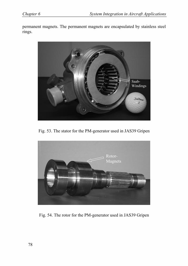
Chapter 6 System Integration in Aircraft Applications
78
permanent magnets. The permanent magnets are encapsulated by stainless steel rings.
Fig. 53. The stator for the PM-generator used in JAS39 Gripen
Fig. 54. The rotor for the PM-generator used in JAS39 Gripen
Saab-Windings
Rotor- Magnets
System Integration in Aircraft Applications Chapter 6
79
6.2 Future Power Systems
Without the restraints of the present standard and the limitation of equipment available from the product catalogs a better weight optimization could be achieved. Airframers are looking into the possibility of using double frequency and double voltage to gain weight. One question to be raised is whether a further increase of the frequency could be beneficial in aircraft electric power design.
Today’s standard for an electric power supply system for an aircraft is in accordance with Mil-Std-704E, which specifies 115V 400 Hz, 28 VDC or 270 VDC. Airframers are currently looking into double frequency (or variable frequency up to 800Hz) and double voltage (3 x 230V AC) or 270 VDC and possibly +/- 270 VDC as the choice for future power supply.
By increasing the frequency, the equipment using magnetic circuits can achieve minimized weight of e.g. generators and transformers. System frequencies in the range of kilo Hertz for missiles, unmanned aerial vehicles (UAV) and other vehicles can be used when size and weight reduction is essential [10].
The alternative, with increased frequency, would give the advantage of reduced weight in the magnetic circuits, such as iron parts in generators, transformers and magnetic amplifiers.
The weight reduction is basically in direct proportion to the increase of frequency. However the full benefit might not be possible due to effects of skin depth and increased impedance in wiring as well as iron losses in the cores.
A Transformer Rectifier Unit (TRU) with the power rating of 3.5 kW, has a weight of 6.8 kg when operating at 400Hz. At 4 kHz the TRU could possibly have a weight less than 1.0 kg. This represents a considerable weight saving. The disadvantage with increased frequency is increased losses due to the skin depth effect and increased reactance in the wiring.
• By increasing the system voltage, the copper area can be reduced. Weight can be saved in the electric power distribution systems.
Chapter 6 System Integration in Aircraft Applications
80
• By allowing variable frequency, the generator system can be simplified, and equipment for controlling the frequency can be excluded. E.g. the constant speed drive (CSD) can be diminished. The CSD represents about half of the weight of the generator. Typical aircraft generators are delivering 115/200 VAC with its frequency regulated to 400 Hz by the CSD. The CSD is commonly used in civil and military aircraft generators and is based on a hydrodynamic design. The leading supplier is Hamilton-Sundstrand, Rockford, IL.
An increased frequency opens new possibilities of using magnetic amplifiers and the equipment using magnetic circuits can be minimized regarding weight. By looking at the equation for designing transformers, E=4.44 • B • A • N • f, it can be understood that generators and transformers can get a lower weight in proportion to the increased frequency.
Beneficial for magamps is that electromagnetic emission (EME) is naturally low due to a soft switching characteristic between saturated and non-saturated state. The requested rectangular hysteresis loop for the magnetic material can be very god, but anything less than perfect implies soft switching and consequently low emissions. This reduces the requirements on the output filtering.
6.2.1 Skin Effect in Wiring The disadvantage with an increased frequency is the skin depth effect allowing only the surface of a wire to be used to conduct the current [45].
The skin depth δ can be expressed:
01
μσπδ f= (6.1)
For a copper wire with the conductivityσ = 5.80 • 107 and a frequency of f= 4000 Hz the skin deep will be approximately 1 mm.
This implies that the center part of the conductor, below 1 mm of the surface does not conduct current.
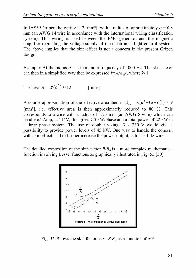
System Integration in Aircraft Applications Chapter 6
81
In JAS39 Gripen the wiring is 2 [mm²], with a radius of approximately a = 0.8 mm (an AWG 14 wire in accordance with the international wiring classification system). This wiring is used between the PMG-generator and the magnetic amplifier regulating the voltage supply of the electronic flight control system. The above implies that the skin effect is not a concern in the present Gripen design.
Example: At the radius a = 2 mm and a frequency of 4000 Hz. The skin factor can then in a simplified way then be expressed k=A/Aeff , where k>1.
The area ≈= )( 2aA π 12 [mm²]
A course approximation of the effective area then is ( ) ≈−−= )( 22 δπ aaAeff 9 [mm²], i.e. effective area is then approximately reduced to 80 %. This corresponds to a wire with a radius of 1.73 mm (an AWG 8 wire) which can handle 65 Amp, at 115V, this gives 7.5 kW/phase and a total power of 22 kW in a three phase system. The use of double voltage 3 x 230 V would give a possibility to provide power levels of 45 kW. One way to handle the concern with skin effect, and to further increase the power output, is to use Litz wire.
The detailed expression of the skin factor R/R0 is a more complex mathematical function involving Bessel functions as graphically illustrated in Fig. 55 [50].
Fig. 55. Shows the skin factor as k=R/R0 as a function of a/δ
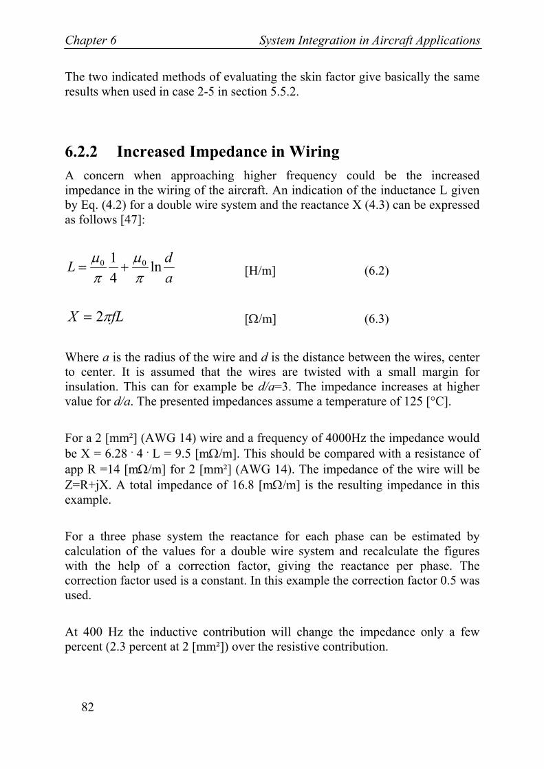
Chapter 6 System Integration in Aircraft Applications
82
The two indicated methods of evaluating the skin factor give basically the same results when used in case 2-5 in section 5.5.2.
6.2.2 Increased Impedance in Wiring A concern when approaching higher frequency could be the increased impedance in the wiring of the aircraft. An indication of the inductance L given by Eq. (4.2) for a double wire system and the reactance X (4.3) can be expressed as follows [47]:
adL ln
41 00
πμ
πμ
+= [H/m] (6.2)
fLX π2= [Ω/m] (6.3)
Where a is the radius of the wire and d is the distance between the wires, center to center. It is assumed that the wires are twisted with a small margin for insulation. This can for example be d/a=3. The impedance increases at higher value for d/a. The presented impedances assume a temperature of 125 [°C].
For a 2 [mm²] (AWG 14) wire and a frequency of 4000Hz the impedance would be X = 6.28 • 4 • L = 9.5 [mΩ/m]. This should be compared with a resistance of app R =14 [mΩ/m] for 2 [mm²] (AWG 14). The impedance of the wire will be Z=R+jX. A total impedance of 16.8 [mΩ/m] is the resulting impedance in this example.
For a three phase system the reactance for each phase can be estimated by calculation of the values for a double wire system and recalculate the figures with the help of a correction factor, giving the reactance per phase. The correction factor used is a constant. In this example the correction factor 0.5 was used.
At 400 Hz the inductive contribution will change the impedance only a few percent (2.3 percent at 2 [mm²]) over the resistive contribution.
System Integration in Aircraft Applications Chapter 6
83
In Fig. 55 it can be noted that the relative impedance at 4000 Hz and 8000 Hz compared to the 400 Hz impedance increases with higher frequency and larger copper area (lower AWG).
In diagram Fig. 56 the absolute value of the wire impedance Z=R+jX is plotted as the total impedance for a wire installation and as a function of the wire area in [mm²].
With the given conditions, it can be noted that the impedance increases approximately by a factor 1.7 for 2 [mm²] (AWG14) when increasing the frequency from 400 Hz to 8000 Hz.
Wire Impedance
0
0,01
0,02
0,03
0,04
0,05
0,06
0,07
0,08
0,4 0,6 1 1,2 2 3 5 9 14 22 34 53Area mm²
Impe
danc
e oh
m/m
400 Hz4000 Hz8000 Hz
Fig. 56. Shows the absolute value of the one phase wire impedance, for a three phase system as a function of the conductor copper area for d/a=3
The increased impedance can not be compensated for by increasing the copper area, since the inductive contribution will increase even if the resistance is
Chapter 6 System Integration in Aircraft Applications
84
lower. At areas larger than this the proportion of the inductive contribution increases.
6.3 Feasible Concepts
A feasible concept comprises a generator supplying the system with a power frequency of e.g. 4000 Hz. A multi pole high-speed generator would offer improved power-density.
With technology of today the power conditioner e.g. a Transformer Rectifier Unit (TRU) working with 400Hz and a power rating of 3.5 kW, has a weight of 6.8 kg. At 4000 Hz the TRU could have a weight less than 1 kg. A considerable weight reduction could evidently be accomplished at higher frequencies.
A general concern in the design of electrical power systems is the power factor. One reason for the concern is the reactive power since this decreases the usable power. This is indicated by the fact that the generators are normally specified in kVA. We produce current and voltage that are not producing effective power, due to the inductive loads and inductive wiring.
The relative increase of inductive voltage loss can be acceptable at lower power levels, around 40 kVA that are suitable for a fighter or an Unmanned Aerial Vehicle (UAV). For a doubled three phase voltage ( 3 x 230V AC) the current peak would be 58 A, giving a voltage drop of approximately 0.5 V/m at 4000 Hz. AC-distribution with the length of 4 m, would still keep the voltage drop within the acceptable limit of 2 V.
In larger aircrafts such as airliners the reactive losses will increase due to increased length of wires that could be in the magnitude of 30 [m] or more. Normally large aircraft are equipped with four or five generators. The power rating of each generator then is as high as 250 kVA. At a doubled voltage the rated current will be as high as 362 A. This current will normally be split on two or three power wires, which offer the advantage of lower reactance (not analysed here).
The proposed concept with a high frequency generator and a power conditioner as shown in Fig. 57, is based on a high frequency distribution system and has the
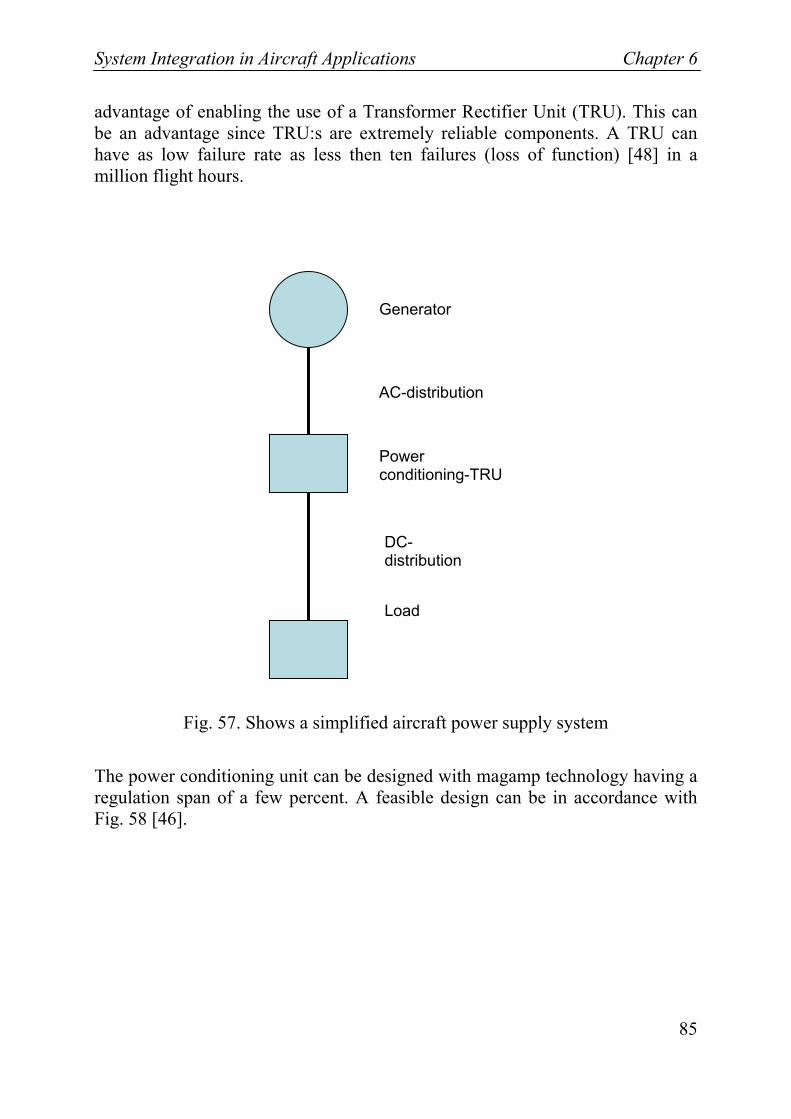
System Integration in Aircraft Applications Chapter 6
85
advantage of enabling the use of a Transformer Rectifier Unit (TRU). This can be an advantage since TRU:s are extremely reliable components. A TRU can have as low failure rate as less then ten failures (loss of function) [48] in a million flight hours.
Fig. 57. Shows a simplified aircraft power supply system
The power conditioning unit can be designed with magamp technology having a regulation span of a few percent. A feasible design can be in accordance with Fig. 58 [46].
Power conditioning-TRU
AC-distribution
DC-distribution
Load
Generator
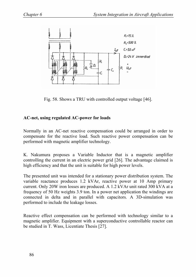
Chapter 6 System Integration in Aircraft Applications
86
Fig. 58. Shows a TRU with controlled output voltage [46].
AC-net, using regulated AC-power for loads
Normally in an AC-net reactive compensation could be arranged in order to compensate for the reactive load. Such reactive power compensation can be performed with magnetic amplifier technology.
K. Nakumura proposes a Variable Inductor that is a magnetic amplifier controlling the current in an electric power grid [26]. The advantage claimed is high efficiency and that the unit is suitable for high power levels. The presented unit was intended for a stationary power distribution system. The variable reactance produces 1.2 kVAr, reactive power at 10 Amp primary current. Only 20W iron losses are produced. A 1.2 kVAr unit rated 300 kVA at a frequency of 50 Hz weights 3.9 ton. In a power net application the windings are connected in delta and in parallel with capacitors. A 3D-simulation was performed to include the leakage losses.
Reactive effect compensation can be performed with technology similar to a magnetic amplifier. Equipment with a superconductive controllable reactor can be studied in T. Wass, Licentiate Thesis [27].
System Integration in Aircraft Applications Chapter 6
87
Reactive compensation for wiring could be performed with series capacitors in order to compensate for the reactive wiring. This can be in combination with reactive compensation.
DC-net, not using regulated AC-power
In a DC-net where no regulated AC current is used reactive voltage drop in the wiring can be accepted. If the generator is unregulated, the voltage might fluctuate due to variation of the input speed of the generator. These voltage variations will be transferred to the accompanying DC-distribution system. A magamp regulator could offer advantages to obtain a constant DC voltage of e.g. 270 VDC.
Regarding DC-systems there are problems to find appropriate circuit breakers, because the physical sizes of such breakers are considerable.
The increased impedance (reactance) due to a higher frequency in the wiring can not be compensated for, by increasing the wire area. In an aircraft installation the distance between phases and distance to structure can be reduced. The voltage can also be increased, which reduces the required size of the wires.
A system optimization should include the impact and effects that the electric power system could have on the other systems; this has been studied in ref [3].
The obtained results show that the magamp technology can offer interesting and competitive systems. The advantages with a magamp application must be evaluated from case to case and the outcome is depending on the specific set of parameters.

Conclusions and Future Work Chapter 7
89
Chapter 7
Conclusions and Future Work
7.1 Conclusions
In this Licentiate thesis magnetic amplifiers and the operation of magnetic amplifiers are discussed. Different concepts are described and analysed by use of a detailed simulation model and proposed engineering tool.
Magnetic amplifiers are a not widely known today. Nevertheless the technology is of interest especially in high reliability applications. The high reliability and robustness also represent a significant value adding to the attraction of magnetic amplifiers in aircraft applications. The primary use today is as voltage regulators. New soft magnetic materials, such as amorphous magnetic alloys, have enabled the use of magnetic amplifier technology in the design of competitive electric power circuits. The studied magnetic amplifiers indicated very high efficiency as well as low weight when operating at high frequencies. The chosen core material is very important for the final result when designing a magamp. The methods for calculating the losses are based on different methods. By using algorithms provided by the vendor or hysteresis models core characteristics and losses is simulated for a proposed design.
By simulation during one or more full cycles of operation of the magamp its behavior can be studied. Electrical data as current and voltage can then be
Chapter 7 Conclusions and Future Work
90
analyzed by studying the hysteresis loops. Based on the flux and magnetic field the iron losses can be analyzed.
The used algorithms and methods to evaluate the losses and specifically the iron losses work very well. The performed simulations indicate very god efficiency of the magamps as well as the feasibility to design them for high power-density.
The model is in this work used to simulate the behavior of a magnetic amplifier and to evaluate losses. The used model can be very useful since it is a dynamic model that can be used for any magnetic amplifier application regardless operating frequency. Furthermore this simulation model of hysteresis losses can be used for any magnetic circuit, as e.g. transformers. The described system integration concepts indicate that the operating conditions for the magnetic amplifiers can offer advantages such as low weight low losses and high reliability.
7.2 Future Work
In further work the models will be verified by comparing the simulated results with tests. Calorimetric analysis is a feasible method to use.
The models need to be updated in accordance with test results.
The models should be extended for a variety of feasible materials of interest, in order to better be able to evaluate suitable alloy for specific applications.
The deviation from perfect squareness of the core magnetization curve is defined by Br/Bs, see Fig 18. It must be considered during design but can according to the reference [28] be compensated for to some extent by the control circuitry. This will be further analyzed in future works.
Saturable reactors may be used as switches to discharge pulsed energy in high power microwave weapons [11]. This and other electric power applications of different magamp circuits are to be evaluated and further studied.
References
91
References
[1] L. Austrin, J.H. Krah and G. Engdahl: “A Modeling Approach of a Magnetic Amplifier”. Proc. of the International Conference of Magnetism, Rome, Italy, 27th July-1st August, 2003.
[2] L. Austrin, and G. Engdahl: “Modeling of a Three-phase Magnetic Amplifier”. Proc. of the 24th Congress of the International Council of the Aeronatical Science, Yokohama, Japan, 29th August-3rd September 2004.
[3] B. Johansson, L. Austrin, G. Engdahl, P. Krus: Tools and Methodology for Collaborative Systems Design Applied on More Electric Aircraft. Proc. ICAS 2004, Yokohama, Japan, 29th August-3rd September 2004.
[4] L. Austrin, J. Hansson: “New Electric Components for Aircraft”, Proc. Flygteknik 2004, Oktober 18-19, 2004 Stockholm (In Swedish).
[5] P. Krus, B. Johansson, L. Austrin: “Concept Optimization of Aircraft Systems Using Scaling Models”. Proc. Recent Advances in Aerospace Actuation Systems and Components, November 24-26, 2004 Toulouse, France.
[6] L. Austrin, D. Ribbenfjärd, G. Engdahl: “Simulation of a Magnetic Amplifier Circuit Including Hysteresis”. Digest for Intermag . Nagoya , Japan, April 2005.
[7] L. Austrin, D. Ribbenfjärd, G. Engdahl: “Simulation of a Magnetic Amplifier Circuit Including Hysteresis”. IEEE transactions.
[8] P Hallberg, L Austrin, P Krus: “Low Cost Demonsatrator as a Mean for Rapid Product Realization with an Electric Motorcycle Application”. Procedings of IDETC/CIE 2005.
[9] M. Howse: “All Electric Aircraft” IEE Power Engineer, Volume 17 Issue: 4, Aug-Sept 2003 pp. 35-37.
[10] G. M. Attura: Magnetic Amplifier Engineering. McGraw-Hill New York 1959.
[11] A. G. Milnes: Transductors and Magnetic Amplifiers. McMillan&Co Ltd-New York, ST Martin's press 1957.
[12] E. R. Hnatek: Design of Solid-State Power Supplies. Van Nostrand Reinhold Company, New York, 1971.
[13] W. A. Geyger: Magnetic Amplifier Circuits. McGraw-Hill, New York, London, 1954.
References
92
[14] H. W. Katz: Solid State Magnetic and Dielectric Devices, John Wiley & Sons Inc 1959.
[15] B. V. Nilsson: Ernst Fredrik Werner Alexandersson. ISBN 91-972360-6-3 [16] A. Bergqvist: Physica B Condensed Matter, Elsevier, 233, p. 342, 1997. [17] D.C. Jiles: “Modelling the Effects of Eddy Current Losses on Frequency
Dependent Hysteresis in Electrically Conducting Media”. IEEE transactions on magnetics vol 30, no 6, nov 1994.
[18] R. Richter: Elektrische Maschinen. Band 1, Birkhauser Verlag, Basel 1951. [19] Metglas product information, www.metglas.com [20] B. Johansson, L. Austrin, G. Engdahl, P. Krus: “Tools and Methodology
for Collaborative Systems Design Applied on More Electric Aircraft”. Proc. ICAS 2004.
[21] Alexander Grimeton, Veteranradions vänner. [22] G. Bertotti: Hysteresis in Magnetism. Academic Press, Inc. 1998, ISBN:0-
12-093270-9 [23] Dymola, www.dynasim.se [24] S. Lemoine: The Alexanderson High frequency Generator. Tekniska
meddelande Kungl. Telegrafstyrelsen Stockholm 1921(In Swedish). [25] Lundahl Transformers, Norrtälje, Sweden [26] K. Nakumura, et al: “Three Dimensional Reluctance Network Analysis
Considering an Iron Loss Characteristic for an EIE-Core Variable Inductor”. Graduate School of Engineering Tohoku University. Proc. ICAS 2004.
[27] T. Wass: Losses in high-temperature superconducting tapes in longitudinally applied magnetic fields. Licentiate Thesis, Stockholm 2003.
[28] R.M. Tedder: ”Limitations of the Magamp Regulator and an Improved Magamp Choke Design Procedure”, Proc. IEEE Applied Power Electronics Conference, 1988 Record, pp. 109 -117
[29] C. Jamerson: “Calculation of Magnetic Amplifier Post Regulator Voltage Control Loop Parameters”, Proceedings of the Second International High Frequency Power Conversion Conference, April, 1987, pp. 222-233.
[30] I. J. Lee, D. Y. Chen, Y. P. Wu, and C. Jamerson: “Modeling of Control Loop Behavior of Magamp Post Regulators”, Proceedings of the Eighth Annual Power Electronics Seminar, Virginia Polytechnic Institute and State University,” September, 1990, pp. 227-234.
[31] D.Y. Chen, J. Lee, and C. Jamerson: “A Simple Model Predicts Small-Signal Control Loop Behavior og Magamp Post
References
93
Regulator”, Proceedings of the Third International High Frequency Power Conversion Conference, San Diego, Ca, May, 1988, pp 69-84
[32] H. Dean Venable: “Practical Techniques for Analyzing, Measuring, and Stabilizing Feedback Control Loops in Switching Regulators and Converters“, Proceedings of the Seventh National Solid-State Power Conversion Conference, Powercon 7 Record, San Diego, CA, March, 1980, pp. I-12.1-I-12.17.
[33] C. Mullett: “New Amorphous Material Improve High-Frequency Saturable Reactor Output Regualtors”, Proc. Power Conversion and Intelligent Motion, July, 1986, pp. 28-35.
[34] G. Engdahl, J. Krah: “Hysteresis model”, Journal of Magnetism and Magnetic Materials, Vol. 242-245, Issue P2, April 2002, pp. 1210-1213.
[35] T.Higuchi: “A Statistical Model of Core Noise in Half-Wave Push-Pull Magnetic Amplifiers”. Proc. IEEE Transactions on Magnetics, Dec 1970.
[36] R. Hiramatsu, et al: “A Magnetic Power Controller of Amorphous Cores for a 200 kHz Switching Regulator”, Proc. IEEE Transactions on Magnetics. vol-18, no.6, Nov 1982.
[37] T. Koyashiki, S. Ohzora: “Control Characteristics in a Magnetic-Amplifier-Controlled DC-DC Converter”. CH 2523-9/88/0000-0390, Proc. IEEE, 1988.
[38] T. Yamaguchi, et al: “Core Noise and an Anomalous Phenomenon in Amorphous Tape Wound Cores used for Sensitive Magnetic Amplifier”, Proc. IEEE Transactions on Magnetics, vol. MAG-22, NO.5, Sept 1986.
[39] M. E. Eaton: “Adding flux paths to SPICEs analytical capability improves the ease and accuracy of simulating power circuits”. Proc. IEEE, 1998.
[40] R. Hiramatsu: “Re-entrant characteristic of Magnetic Amplifier A New Analysis”, Proc. IEEE, 1988.
[41] K. Murakami: “An Experimental Study of Flux Presetting-Resetting Characteristics of Magnetic Cores with Rectangular Hysteresis Loop”, Proc. IEEE Transactions on Magnetics, 1965.
[42] K. Harada: “Applications of Magnetic Amplifiers to High-Frequency DC-to DC Converters”. Proceedings of the IEEE, vol-76, no.4, April 1988.
[43] C. Jamerson: “Techniques for Reduction of Required Hearoom in High-Frequency Magamp Postregulators”, IEEE Transactions of Power Electronics, vol-8, no.1, January 1993.
References
94
[44] S. Nakajima: “Loss Evaluation of Amorphous Saturable-Core”, IEEE Transactions on Magnetics, vol. MAG-23, no.5, Sept 1987.
[45] S. Ramo, J. R. Whinner, T. van Duzer: Fields and Waves in Communication Electronics. John Wiley & sons, New York, 1965, pp. 288-293.
[46] D. Eckerström: JAS39 a Regulated Transformer Rectifier Unit, Master Thesis, Chalmers, Gothenburg, 1993 (In Swedish)
[47] E. Hallén: Electromagnetic Theory. Chapman & Hall, London, 1965, pp. 250-252.
[48] EuroAtlas, Bremen, “TRU-product information” [49] P. Westberg: ”Lundahl och den magnetiska förstärkaren”, High Fidelity, no
3, 1997, pp. 18-20. Audio Media A/S Kopenhagen, Denmark (In Swedish). [50] Scots: Guide audio skineffect, pp.1. www.st-andrews.ac.uk
List of Symbols
95
List of Symbols
Symbol Quantity Unit A Area [m²] ACu Cross-section area of the conductor, copper [m2] a Radius of the wire [m] B Magnetic flux density (Tesla [T] = [Vs/m²]) [T] Br Residual magnetic flux density [T] Bs Saturation magnetic flux density [T] $B Amplitude of the mean flux density [T]
Dm Inner diameter [m] d Distance between conductors [m] d Ribbon thickness of core material [m] f Frequency [Hz] G Parameter of magnetic domains [ - ] H Magnetic field [A/m] Hc Coercivity force [A/m] hFe Flux path length [m] I Current [A] J Current density [A/m²] kwindFactor Winding factor [ - ] k Skin factor [ - ] kh Empiric constant, hysteresis losses [ - ] Ltot Total inductance [H] l Length [m] m Mass [kg] N Number of turns [ - ] P Power loss [W] Piron Power losses, iron [W] PCU Power losses, copper [W] p Number of phases [ - ] R Resistance [ohm] R Reluctance [A/Vs] T Temperature [°C] T Cycle time [s] t Time [s]
List of Symbols
96
U Voltage [V] V Volume [m³] W Energy [Ws] w Width of the core ribbon [m] X Reactance [Ω] Ze Impedance, electrical [Ω] δ Skin depth [m] η Efficiency [ - ] Θ MMF [A] µr Relative permeability [ - ] µ0 Permeability constant [Vs/Am] ρRes,Cu Resistivity of copper [Ωm]
ρdensity Material density 3
kgm⎡ ⎤⎢ ⎥⎣ ⎦
σ Conductivity of the material [1/ohmm] Ø Magnetic flux [Wb] = [Vs] Ω Resistance, conduction [ ]Ω
Appendix
97
Appendix
H 1[Oe] = 10³ / 4 π [A/m] B Magnetic flux density Tesla [T] = [Vs/m²] Gauss 1[G] = 10-4 [T] µ0 Permeability for vacuum =4 π • 10-7 [Vs/Am]
Index
98
Index
Alexanderson, 3, 6, 92 Alloys, 27 Amorphous, II, 93, 94 Anhysteretic, 45, 46 Annealing, 30, 31 ASEA, 8 Bertotti, 47, 49, 92 Calorimetric, 90 Coercivity, 25, 95 Coercivity force, 25, 95 Compliance, 35, 50, 60 Constant, II, 32, 33, 34, 46, 80, 82, 87, 95, 96 Current, 3, 9, 13, 14, 15, 17, 18, 19, 21, 23, 24, 30,
31, 33, 43, 55, 56, 57, 58, 59, 64, 66, 67, 68, 71, 73, 74, 80, 84, 86, 87, 89, 92, 95
Design, I, 1, 2, 8, 9, 10, 11, 13, 15, 22, 23, 24, 26,
27, 29, 37, 43, 66, 67, 68, 69, 73, 74, 75, 77, 79, 80, 81, 84, 85, 89, 90, 91, 92
Dymola, II, 10, 49, 92 Eddy current, I, 9, 11, 31, 33, 34, 47, 48, 49 Efficiency, 9, 27, 41, 55, 59, 66, 70, 73, 74, 86, 89,
90, 96 Energy, 32, 34, 90, 96 Equivalent, 43, 44, 48 Equivalent circuit, 44 Experimental, 50, 75, 93 Flux, 68, 73, 93, 95 Flux density, 9, 22, 25, 32, 33, 60, 61, 62, 66, 74,
95, 97 Frequency, I, 2, 3, 5, 6, 7, 8, 9, 11, 22, 32, 33, 34,
46, 60, 61, 64, 66, 68, 70, 71, 73, 74, 77, 79, 80, 81, 82, 83, 84, 86, 87, 90, 92, 93, 95
Generator, II, 92 Grimeton, 3, 4, 5, 6, 7, 92 Gripen, I, 1, 2, 24, 37, 38, 40, 77, 78, 81 Impedance, 7, 79, 82, 83, 87, 96 Inductance, 21, 43, 82, 95 Lamination, 96 Magnetic circuit, I, 3, 79, 80, 90 Magnetisation, 5, 45, 46 MEA, II, 1, 9 Methods, 2, 75, 89, 90 Permeability, 27, 30, 96, 97 Play operator, 45, 46 Power, I, II, 1, 2, 3, 6, 7, 8, 9, 10, 11, 13, 14, 15, 17,
19, 20, 22, 23, 24, 26, 31, 32, 33, 34, 38, 52, 53, 54, 55, 56, 57, 58, 59, 61, 66, 67, 69, 73, 74, 77, 79, 81, 84, 85, 86, 87, 89, 90, 91, 92, 93, 95
Pseudo particle, 45 Ramey, 8, 19, 20, 21, 22, 26, 69 Reluctance, 92, 95 Resistance, 7, 21, 64, 74, 82, 83, 95, 96 Resistive losses, 75 Short circuit, 7 Simulation, I, II, 9, 10, 12, 43, 49, 50, 51, 52, 55,
56, 57, 58, 59, 74, 75, 86, 89, 90, 91 Steinmetz, 3, 33 Temperature, 24, 55, 68, 82, 92 Voltage, 68, 73, 92, 96