EPA 600/R-04/101September, 2004

On-line Tools for Assessing Petroleum Releases

by

James W. WeaverEcosystems Research Division

National Exposure Research LaboratoryAthens, Georgia 30605

National Exposure Research LaboratoryOffice of Research and Development

U.S. Environmental Protection AgencyResearch Triangle Park, NC 27711

ii

Notice

The U.S. Environmental Protection Agency through its Office of Research and Developmentfunded and managed the research described here. It has been subjected to the Agency’s peer andadministrative review and has been approved for publication as an EPA document. Mention oftrade names or commercial products does not constitute endorsement or recommendation for use.

The author acknowledges contributions and interactions with colleagues in the New York StateDepartment of Environmental Conservation, Pennsylvania Land Recycling Program, NorthCarolina Department of Natural Resources, Ohio Bureau of Underground Storage TankRegulations, Delaware Department of Natural Resources and Environmental Control, WisconsinDepartment of Natural Resources , EPA Regions 9 and 4.

iii

Foreword

The National Exposure Research Laboratory’s Ecosystems Research Division (ERD) in Athens,Georgia, conducts research on organic and inorganic chemicals, greenhouse gas biogeochemicalcycles, and land use perturbations that create direct and indirect, chemical and non-chemicalstresses, exposures, and potential risks to humans and ecosystems. ERD develops, tests, appliesand provides technical support for exposure and ecosystem response models used for assessingand managing risks to humans and ecosystems, within a watershed / regional context.

The Regulatory Support Branch (RSB) conducts problem-driven and applied research, developstechnology tools, and provides technical support to customer Program and Regional Offices,States, Municipalities, and Tribes. Models are distributed and supported via the EPA Center forExposure Assessment Modeling (CEAM).

The Internet tools described in this report provide methods and models for evaluation ofcontaminated sites. Two problems are addressed by models. The first is the placement of wellsfor correct delineation of contaminant plumes. Because aquifer recharge can displace plumesdownward, the vertical placement of well screens is critical to obtain proper characterizationdata. The second is the use of models where data are limited. In this case some form ofuncertainty analysis is necessary to evaluate transport behavior. The remainder of the reportdescribes a series of tools for estimating various model input parameters.

Rosemarie C. Russo, Ph.D.DirectorEcosystems Research DivisionAthens, Georgia

iv

Table of Contents

Notice . . . . . . . . . . . . . . . . . . . . . . . . . . . . . . . . . . . . . . . . . . . . . . . . . . . . . . . . . . . . . . . . . . . . . . ii

Foreword . . . . . . . . . . . . . . . . . . . . . . . . . . . . . . . . . . . . . . . . . . . . . . . . . . . . . . . . . . . . . . . . . . . iii

List of Figures . . . . . . . . . . . . . . . . . . . . . . . . . . . . . . . . . . . . . . . . . . . . . . . . . . . . . . . . . . . . . . . vi

List of Tables . . . . . . . . . . . . . . . . . . . . . . . . . . . . . . . . . . . . . . . . . . . . . . . . . . . . . . . . . . . . . . . viii

1. Introduction . . . . . . . . . . . . . . . . . . . . . . . . . . . . . . . . . . . . . . . . . . . . . . . . . . . . . . . . . . . . . . . . 1The On-line Calculators . . . . . . . . . . . . . . . . . . . . . . . . . . . . . . . . . . . . . . . . . . . . . . . . . . . 1

2. Plume Diving . . . . . . . . . . . . . . . . . . . . . . . . . . . . . . . . . . . . . . . . . . . . . . . . . . . . . . . . . . . . . . 3Vertical Delineation and Transport of Contaminants . . . . . . . . . . . . . . . . . . . . . . . . . . . . 3

1) East Patchogue, New York Plume Diving . . . . . . . . . . . . . . . . . . . . . . . . . . . . . 42) Average Borehole Concentration Calculator . . . . . . . . . . . . . . . . . . . . . . . . . . . 6

The Embedded Data . . . . . . . . . . . . . . . . . . . . . . . . . . . . . . . . . . . . . . . . . . 8Calculation Method . . . . . . . . . . . . . . . . . . . . . . . . . . . . . . . . . . . . . . . . . . 9

Example Results . . . . . . . . . . . . . . . . . . . . . . . . . . . . . . . . . . . . . . 93) Observation of Vertical Gradients . . . . . . . . . . . . . . . . . . . . . . . . . . . . . . . . . . 11

Well Cluster Example . . . . . . . . . . . . . . . . . . . . . . . . . . . . . . . . . . . . . . . 14Application to Plume Diving . . . . . . . . . . . . . . . . . . . . . . . . . . . . . . . . . . 15

Recharge-Driven Plume Diving Calculation . . . . . . . . . . . . . . . . . . . . . . . . . . . . 16Theory . . . . . . . . . . . . . . . . . . . . . . . . . . . . . . . . . . . . . . . . . . . . . . . . . . . 17East Patchogue Example . . . . . . . . . . . . . . . . . . . . . . . . . . . . . . . . . . . . . 18Required Input . . . . . . . . . . . . . . . . . . . . . . . . . . . . . . . . . . . . . . . . . . . . . 19

Flow System Hydraulics . . . . . . . . . . . . . . . . . . . . . . . . . . . . . . . 19Source and Observation Well Locations . . . . . . . . . . . . . . . . . . . 20Model Results . . . . . . . . . . . . . . . . . . . . . . . . . . . . . . . . . . . . . . . 21Drawing Options . . . . . . . . . . . . . . . . . . . . . . . . . . . . . . . . . . . . . 21

3 Contaminant Transport . . . . . . . . . . . . . . . . . . . . . . . . . . . . . . . . . . . . . . . . . . . . . . . . . . . . . . 22First Arrival Versus Advective Travel Times . . . . . . . . . . . . . . . . . . . . . . . . . . . 22

Uncertainty Range Determination . . . . . . . . . . . . . . . . . . . . . . . . . . . . . . 26Approach . . . . . . . . . . . . . . . . . . . . . . . . . . . . . . . . . . . . . . . . . . . 27Simulation . . . . . . . . . . . . . . . . . . . . . . . . . . . . . . . . . . . . . . . . . . 29Results . . . . . . . . . . . . . . . . . . . . . . . . . . . . . . . . . . . . . . . . . . . . . 30

Concentration Uncertainty Model Input and Output . . . . . . . . . . . . . . . . . . . . . . 34

4. Model Input Parameters . . . . . . . . . . . . . . . . . . . . . . . . . . . . . . . . . . . . . . . . . . . . . . . . . . . . . 37Retardation Factor Calculator . . . . . . . . . . . . . . . . . . . . . . . . . . . . . . . . . . . . . . . . . . . . . 37

v

Example . . . . . . . . . . . . . . . . . . . . . . . . . . . . . . . . . . . . . . . . . . . . . . . . . . . . . . . . 38Ground Water Velocity . . . . . . . . . . . . . . . . . . . . . . . . . . . . . . . . . . . . . . . . . . . . . . . . . . 39

Seepage Velocity Calculator . . . . . . . . . . . . . . . . . . . . . . . . . . . . . . . . . . . . . . . . 39Hydraulic Gradient Calculator . . . . . . . . . . . . . . . . . . . . . . . . . . . . . . . . . . . . . . . 40

Example . . . . . . . . . . . . . . . . . . . . . . . . . . . . . . . . . . . . . . . . . . . . . . . . . . 40Longitudinal Dispersion Coefficient Calculator . . . . . . . . . . . . . . . . . . . . . . . . . . . . . . . 43Half-Lives to Rate Constant Conversion Calculator . . . . . . . . . . . . . . . . . . . . . . . . . . . . 46Effective Solubility from Mixture Calculator . . . . . . . . . . . . . . . . . . . . . . . . . . . . . . . . . 47

Shallow Ground Water Temperature in the United States . . . . . . . . . . . . . . . . . . 47Temperature Dependence of MTBE, Benzene and Toluene Solubility . . . . . . . . 48

MTBE . . . . . . . . . . . . . . . . . . . . . . . . . . . . . . . . . . . . . . . . . . . . . . . . . . . 49Benzene . . . . . . . . . . . . . . . . . . . . . . . . . . . . . . . . . . . . . . . . . . . . . . . . . . 49Toluene . . . . . . . . . . . . . . . . . . . . . . . . . . . . . . . . . . . . . . . . . . . . . . . . . . 52Example Values . . . . . . . . . . . . . . . . . . . . . . . . . . . . . . . . . . . . . . . . . . . . 53Temperature-Dependent Henry’s Law Coefficient Calculator . . . . . . . . 55

Example Values . . . . . . . . . . . . . . . . . . . . . . . . . . . . . . . . . . . . . . . . . . . . . . . . . . 56Diffusion Coefficient Calculator . . . . . . . . . . . . . . . . . . . . . . . . . . . . . . . 58

5. Conclusions . . . . . . . . . . . . . . . . . . . . . . . . . . . . . . . . . . . . . . . . . . . . . . . . . . . . . . . . . . . . . . . 60

References . . . . . . . . . . . . . . . . . . . . . . . . . . . . . . . . . . . . . . . . . . . . . . . . . . . . . . . . . . . . . . . . . . 61

Appendix 1 Calculator Reference . . . . . . . . . . . . . . . . . . . . . . . . . . . . . . . . . . . . . . . . . . . . . . . . 64

Appendix 2 Acronyms and Abbreviations . . . . . . . . . . . . . . . . . . . . . . . . . . . . . . . . . . . . . . . . . 65

Appendix 3 Plume Diving Calculator Equations . . . . . . . . . . . . . . . . . . . . . . . . . . . . . . . . . . . . . 66

Appendix 4 One-Dimensional Transport in a Homogeneous Aquifer . . . . . . . . . . . . . . . . . . . . 69

Appendix 5 Estimation of Temperature-Dependent Henry’s Law Coefficients . . . . . . . . . . . . . 71

Appendix 6 Diffusion Coefficients . . . . . . . . . . . . . . . . . . . . . . . . . . . . . . . . . . . . . . . . . . . . . . . 73

vi

List of Figures

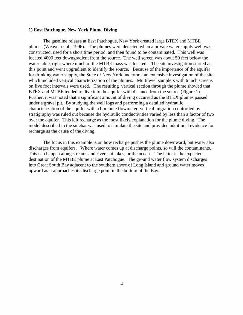
Figure 1 Vertical cross section through the MTBE, and benzene plumes. The gasoline source islocated at the right hand edge of the sections and flow is to the left. Each of the plumesdives into the aquifer with transport in the aquifer. . . . . . . . . . . . . . . . . . . . . . . . . . . . . . . 4

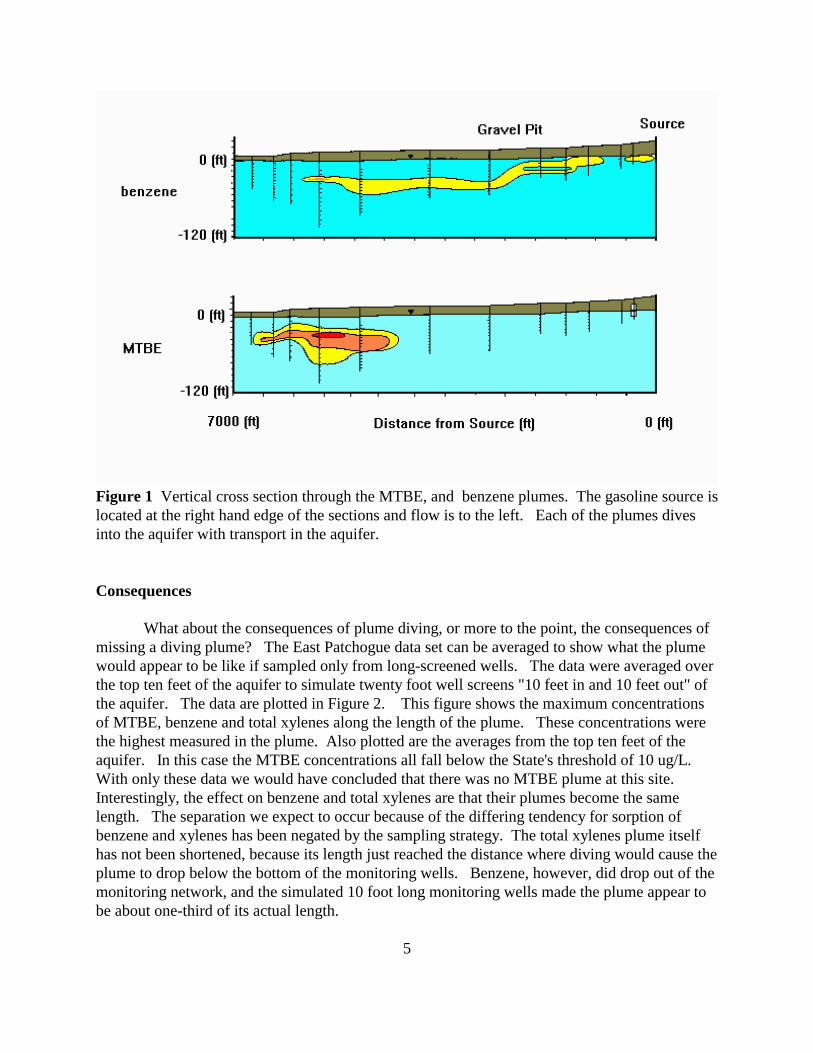
Figure 2 Consequences of sampling only the top ten feet of the aquifer at East Patchogue, NewYork. The MTBE plume would disappear (top); the benzene plume would be shortenedby two thirds; and the total xylenes plume appears at the same length because its extentdid not reach the gravel pit where diving dominates the contaminant distribution. . . . . . 6

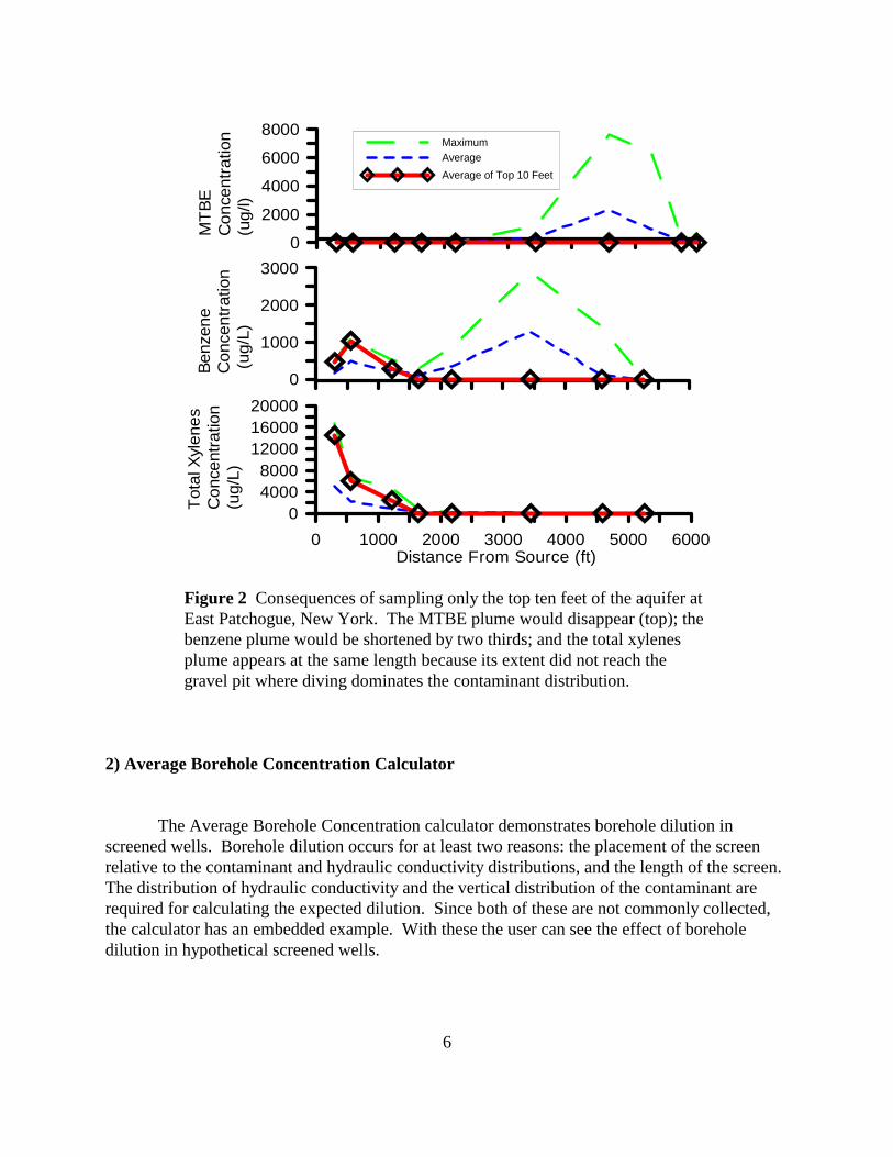
Figure 3 Average borehole concentration calculation. . . . . . . . . . . . . . . . . . . . . . . . . . . . . . . . . . 6Figure 4 Illustration of components of borehole flow calculator graphics. . . . . . . . . . . . . . . . . . 8Figure 5 Estimated borehole concentration

of 120 :g/L for a twenty-foot long well screen located 20 feet below the land surface.. . . . . . . . . . . . . . . . . . . . . . . . . . . . . . . . . . . . . . . . . . . . . . . . . . . . . . . . . . . . . . . . . . . . . 10

Figure 6 Estimated borehole concentration of 5677 :g/L for a five-foot well screen located 50feet below the land surface. . . . . . . . . . . . . . . . . . . . . . . . . . . . . . . . . . . . . . . . . . . . . . . . 10

Figure 7 Estimated borehole concentration of 995 :g/L for a ten-foot long well screen placed 70feet below the land surface. . . . . . . . . . . . . . . . . . . . . . . . . . . . . . . . . . . . . . . . . . . . . . . . 10

Figure 8 Definition of relationships for vertical gradient calculations: dw is the depth to water, dthe depth to the top of the well screen, and s is the screen length. . . . . . . . . . . . . . . . . . 11

Figure 9 Submerged, water table and dry conditions of a well screen. . . . . . . . . . . . . . . . . . . . . 11Figure 10 Assumed distances for vertical gradient calculation: H = high, M=medium, L=low.

. . . . . . . . . . . . . . . . . . . . . . . . . . . . . . . . . . . . . . . . . . . . . . . . . . . . . . . . . . . . . . . . . . . . . 12Figure 11 Gradients in wells that are screened in heterogeneous materials. . . . . . . . . . . . . . . . . 13Figure 12 Input and output screen for the plume diving calculator. . . . . . . . . . . . . . . . . . . . . . . 16Figure 13 Example plume diving calculation for the East Patchogue site. . . . . . . . . . . . . . . . . 18Figure 14 Plume Diving calculator hydraulic and hydrologic property entry. . . . . . . . . . . . . . . 19Figure 15 Plume Diving calculator location entry. . . . . . . . . . . . . . . . . . . . . . . . . . . . . . . . . . . . 20Figure 16 Plume Diving calculator graphical output. . . . . . . . . . . . . . . . . . . . . . . . . . . . . . . . . . 20Figure 17 Plume Diving calculator mass balance output. . . . . . . . . . . . . . . . . . . . . . . . . . . . . . . 21Figure 18 Plume Diving calculator display options. . . . . . . . . . . . . . . . . . . . . . . . . . . . . . . . . . . 21Figure 19 Illustration of transport by advection only (hypothetical) and transport by advection

and dispersion. . . . . . . . . . . . . . . . . . . . . . . . . . . . . . . . . . . . . . . . . . . . . . . . . . . . . . . . . . 23Figure 20 Illustration showing the relationship between the first arrival time, maximum

concentration and duration of contamination. The first arrival time and duration aredetermined relative to a given threshold concentration, that is usually a maximumcontaminant level or other concentration of concern. . . . . . . . . . . . . . . . . . . . . . . . . . . . 24

Figure 21 Relationship of uncertainty to model data availability. . . . . . . . . . . . . . . . . . . . . . . . 26Figure 22 Output from the Concentration Uncertainty applet showing the wide range of

breakthrough curves that are possible given specified ranges of input parameters. . . . . 28Figure 23 Fixed parameters required for the Concentration Uncertainty model. . . . . . . . . . . . . 34Figure 24 Potentially variable parameters required for the Concentration Uncertainty model.

. . . . . . . . . . . . . . . . . . . . . . . . . . . . . . . . . . . . . . . . . . . . . . . . . . . . . . . . . . . . . . . . . . . . . 34

vii

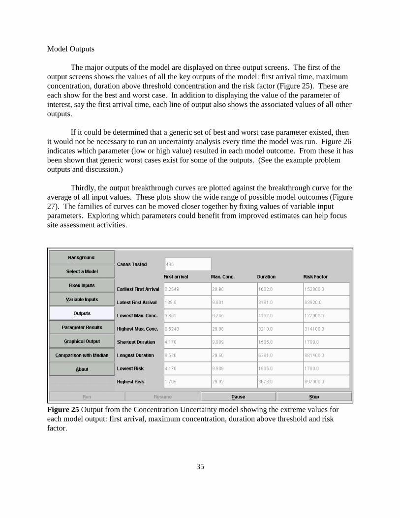
Figure 25 Output from the Concentration Uncertainty model showing the extreme values foreach model output: first arrival, maximum concentration, duration above threshold andrisk factor. . . . . . . . . . . . . . . . . . . . . . . . . . . . . . . . . . . . . . . . . . . . . . . . . . . . . . . . . . . . . 35

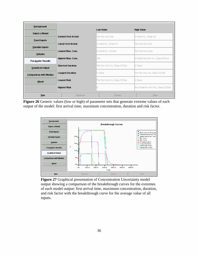
Figure 26 Generic values (low or high) of parameter sets that generate extreme values of eachoutput of the model: first arrival time, maximum concentration, duration and risk factor.. . . . . . . . . . . . . . . . . . . . . . . . . . . . . . . . . . . . . . . . . . . . . . . . . . . . . . . . . . . . . . . . . . . . . 35

Figure 27 Graphical presentation of Concentration Uncertainty model output showing acomparison of the breakthrough curves for the extremes of each model output: firstarrival time, maximum concentration, duration, and risk factor with the breakthroughcurve for the average value of all inputs. . . . . . . . . . . . . . . . . . . . . . . . . . . . . . . . . . . . . . 36

Figure 28 Magnitude and direction of gradient for example site. . . . . . . . . . . . . . . . . . . . . . . . . 40Figure 29 Data tabulation from Gelhar et al. (1992) showing published longitudinal dispersivity

as a function of scale. . . . . . . . . . . . . . . . . . . . . . . . . . . . . . . . . . . . . . . . . . . . . . . . . . . . . 43Figure 30 Gelhar et al. (1992) dispersivity tabulation with scale-related estimates. . . . . . . . . . 44Figure 31 Shallow ground water temperatures throughout the United States. . . . . . . . . . . . . . . 47Figure 32 Graph of MTBE solubility versus temperature showing decline in solubility with

increasing temperature. . . . . . . . . . . . . . . . . . . . . . . . . . . . . . . . . . . . . . . . . . . . . . . . . . . 48Figure 33 Graph of benzene solubility versus temperature showing modest increase in solubility

with increasing temperature. . . . . . . . . . . . . . . . . . . . . . . . . . . . . . . . . . . . . . . . . . . . . . . 49Figure 34 IUPAC data on benzene solubility showing the lower 95% confidence limit,

recommended value, and upper 95% confidence limit. . . . . . . . . . . . . . . . . . . . . . . . . . . 51Figure 35 IUPAC data on toluene solubility showing the lower value, best value, and upper

value. . . . . . . . . . . . . . . . . . . . . . . . . . . . . . . . . . . . . . . . . . . . . . . . . . . . . . . . . . . . . . . . . 52Figure 36 Water table mounding due to unequal recharge and hydraulic conductivity. . . . . . . 67

viii

List of Tables

Table 1 Effects of well screen length on concentrations given in :g/L observed wells screenedfrom 20 feet to 90 feet below the land surface at East Patchogue, New York. . . . . . . . . 10

Table 2 Example field data for vertical gradient determination. . . . . . . . . . . . . . . . . . . . . . . . . . 14Table 3 Example gradient estimates indicating the smallest, midpoint to midpoint, highest and

the value for a piezometer. . . . . . . . . . . . . . . . . . . . . . . . . . . . . . . . . . . . . . . . . . . . . . . . . 15Table 4 Gradient magnitude for a difference in head of 0.01 ft and various distances between

well screens. . . . . . . . . . . . . . . . . . . . . . . . . . . . . . . . . . . . . . . . . . . . . . . . . . . . . . . . . . . . 15Table 5 Parameter inputs, their treatment in the model as fixed or variable and the values used

in the model uncertainty example. . . . . . . . . . . . . . . . . . . . . . . . . . . . . . . . . . . . . . . . . . . 28Table 6 The problem definition, its treatment in the model as fixed or variable and the values

used in the uncertainty example. . . . . . . . . . . . . . . . . . . . . . . . . . . . . . . . . . . . . . . . . . . . 29Table 7 Model results for four scenarios showing a comparison of best and worst cases for the

four outputs (first arrival time, maximum concentration, duration and risk). . . . . . . . . . 31Table 8 Comparison of data sets giving the worst cases for each of four model outputs. . . . . 32Table 9 Retardation factors for benzene under varying conditions. . . . . . . . . . . . . . . . . . . . . . . 38Table 10 Retardation factors for MTBE under varying conditions. . . . . . . . . . . . . . . . . . . . . . . 39Table 11 Data for gradient calculation example. . . . . . . . . . . . . . . . . . . . . . . . . . . . . . . . . . . . . 41Table 12 Relationships between plume length, data scatter on the Gelhar (1992) tabulation and

the Xu and Eckstein (1995) formula. . . . . . . . . . . . . . . . . . . . . . . . . . . . . . . . . . . . . . . . . 45Table 13 IUPAC benzene solubility data. . . . . . . . . . . . . . . . . . . . . . . . . . . . . . . . . . . . . . . . . . . 50Table 14 IUPAC toluene solubility data. . . . . . . . . . . . . . . . . . . . . . . . . . . . . . . . . . . . . . . . . . . 52Table 15 Example effective solubilities for benzene and MTBE at temperatures of 5oC, 15oC

and 25 oC. . . . . . . . . . . . . . . . . . . . . . . . . . . . . . . . . . . . . . . . . . . . . . . . . . . . . . . . . . . . . . 53Table 16 Range of variation of effective solubilities for benzene and MTBE from 5oC to 25 oC.

. . . . . . . . . . . . . . . . . . . . . . . . . . . . . . . . . . . . . . . . . . . . . . . . . . . . . . . . . . . . . . . . . . . . . 54Table 17 Unit sets for Henry’s Constants. . . . . . . . . . . . . . . . . . . . . . . . . . . . . . . . . . . . . . . . . 56Table 18 Constants needed for Henry’s law unit conversions. . . . . . . . . . . . . . . . . . . . . . . . . . . 56Table 19 Estimated Henry’s law coefficients for benzene, MTBE, perchloroethene and

trichloroethene at temperatures of 5 oC, 15 oC, and 25 oC. . . . . . . . . . . . . . . . . . . . . . . . 57Table 20 Diffusion coefficient calculation input parameters for benzene, MTBE,

perchloroethene, and trichlorethene. . . . . . . . . . . . . . . . . . . . . . . . . . . . . . . . . . . . . . . . . 58Table 21 Estimated air and water diffusivities for benzene, MTBE, perchloroethene and

trichloroethene at temperatures of 5 oC, 15 oC, and 25 oC. . . . . . . . . . . . . . . . . . . . . . . . 59Table 22 Web (URLs) for models and associated calculations described in the text. . . . . . . . . 64Table 23 Web (URLs) for formulas/model inputs described in the text. . . . . . . . . . . . . . . . . . . 64Table 24 Exponent “n” used in calculation of enthalpy of vaporization. . . . . . . . . . . . . . . . . . 71

1Use of the calculators require that Javascript be enabled and that the Java 2 plug-in beavailable. See http://www.java.com/en/download/windows_automatic.jsp for more information.

2Other significant interactions have occurred with the North Carolina Department ofNatural Resources, Ohio Bureau of Underground Storage Tank Regulations, DelawareDepartment of Natural Resources and Environmental Control, Wisconsin Department of NaturalResources , EPA Regions 9 and 4.

1

1. Introduction

Sites that are contaminated with fuels and dissolved components of petroleum productsare commonly assessed through a combination of field data collection and application of models. The field data typically consist of two types: first, field-measured aquifer parameters andsecond, contaminant and water level observations. The first type may consist of grain sizedistributions, hydraulic conductivity, and aquifer geometry. The second, contaminant and waterlevel data, may consist of soil core data, aqueous concentrations, water and product levels inwells. Generally the second type of data is most abundant. The distinction between the twotypes of data is made because the first type of data correspond, even if roughly, to inputs tomodels and the second type to outputs from models.

Rarely are field data alone used in assessing a site. Some means are needed to extractinformation from the data. Usually this is done with models of various types. Models may takethe form of simple formulas or complex numerical calculations. The simpler formulas andapproaches may not be perceived as models, but they share similar characteristics. Each is basedupon a set of assumptions which in some cases are well-matched by site conditions. Generallyeach also require ancillary data which are often obtained from the literature. In some cases theseancillary data are not easily obtained. The purpose of the methods and models described in thisreport provide a basis for evaluating field observations and extracting information from a varietyof field observations.

The On-line Calculators

Each of the methods and models described in this document are available as a set of on-line calculators. They may be found on the Internet1 at:

http://www.epa.gov/athens/onsite

The calculators were developed from interactions with state environmental agencies. The mostimportant collaborations have been with the Region 2 Office of the New York State Departmentof Environmental Conservation and the Pennsylvania Land Recycling program2.

Four types of calculations are found on the web site:

2

• formulas,• models,• scientific demos, and• unit conversions.

The formulas generally represent inputs to transport models that are derived from fieldobservations, literature data, or a combination of the two. These address concepts of field dataassessment discussed in the Introduction. The models are intended to transfer knowledge gainedfrom working on various sites. Because of limitations inherent to use of the Internet, it is notdesirable to reproduce complex models as web applications. Primarily the ability to store data isseverely restricted. The models are thus simple, but intended to introduce important concepts,rather than serve as competitors to PC models. The term “calculator” also represents the models,because they are intermediate between a hand calculation and a complex modeling application.

Two of the models have been selected for highlighting in this report. These appear inChapters 2 and 3. The first model addresses the diving of contaminant plumes into aquifers. This behavior may be caused by recharge of rainwater. In light of the uncertainties in modelparameters, this calculation is not expected to give some sort of exact answer, but is intended tobe used to place well screens in the best possible vertical positions.

The second of the models is called “ConcentrationUncertainty” because it addresses theranges of possible model behavior given uncertainty in model input parameters. As will bedescribed, each parameter of the model is subject to some amount of uncertainty and thisapplication highlights that uncertainty. To move beyond simply identifying this problem, themodel can also determine generic parameter sets that always produce the worst (or best) caseresults. For some applications, single model runs with these parameters could be used for morecertain decision-making, than the typical average parameter values used by modelers.

The remainder of the document (Chapter 4) is devoted to describing specific inputs tomodels, focusing on those that drive transport. Each of these calculations is described, alongwith literature and other input data. For each method an examination of typical results is given. For reference, Appendix 1 gives the Internet addresses for each calculator described in the text.

3The Average Borehole Concentration calculator:http://www.epa.gov/athens/learn2model/part-two/onsite/abc.htm.

4The Vertical Gradient calculator: http://www.epa.gov/athens/learn2model/part-two/onsite/vgradient.htm.

5The Plume Diving calculator: http://www.epa.gov/athens/learn2model/part-two/onsite/diving.htm.

3

2. Plume Diving

This chapter describes the first of two models and its approach to their site-specific usage. The first model was designed to aid in the placement of monitoring wells by assessing thecontribution of aquifer recharge to the vertical position of contaminant plumes. This topic willintroduced through data from a site and three on-line tools. The on-line tools allow explorationof the apparent concentrations in boreholes that result from screen length and well placementchoices3, the estimation of vertical gradients from nested wells4, and the approximation ofvertical displacement of plumes due to aquifer recharge.5 The first two of these calculatorsintroduce the issues of vertical transport and the third allows site-specific data to be used forestimating plume diving and subsequent placement of well screens.

Vertical Delineation and Transport of Contaminants

Primarily contaminants are transported by flowing ground water. Thus the direction thatthe contaminant takes is determined by the direction of the flowing ground water. When groundwater moves deeper into an aquifer, the contaminants are also transported deeper or “dive”. Thishas an implication for sampling and well construction: the sample intervals must be locatedappropriately or diving plumes might be missed.

Data from the East Patchogue, New York gasoline release site (Weaver et al., 1996) areused to illustrate the consequences of ill-placed well screens. At this site there was an intensivecharacterization using vertically-discrete samplers. As a result the vertical distribution ofcontaminants is well-known. The second example is derived from this data and allowsplacement of well screens of differing lengths at differing depths in the aquifer. Byencapsulating this idea in an applet, the implications of screen length and position can be seendirectly from a data set.

These examples illustrate problems that can be created by inappropriate samplinglocations. A simple calculation may assist in estimating the required placement of monitoringwells when recharge dominates vertical flow. This calculation is available in a calculator that isdescribed below.

4

1) East Patchogue, New York Plume Diving

The gasoline release at East Patchogue, New York created large BTEX and MTBEplumes (Weaver et al., 1996). The plumes were detected when a private water supply well wasconstructed, used for a short time period, and then found to be contaminated. This well waslocated 4000 feet downgradient from the source. The well screen was about 50 feet below thewater table, right where much of the MTBE mass was located. The site investigation started atthis point and went upgradient to identify the source. Because of the importance of the aquiferfor drinking water supply, the State of New York undertook an extensive investigation of the sitewhich included vertical characterization of the plumes. Multilevel samplers with 6 inch screenson five foot intervals were used. The resulting vertical section through the plume showed thatBTEX and MTBE tended to dive into the aquifer with distance from the source (Figure 1). Further, it was noted that a significant amount of diving occurred as the BTEX plumes passedunder a gravel pit. By studying the well logs and performing a detailed hydrauliccharacterization of the aquifer with a borehole flowmeter, vertical migration controlled bystratigraphy was ruled out because the hydraulic conductivities varied by less than a factor of twoover the aquifer. This left recharge as the most likely explanation for the plume diving. Themodel described in the sidebar was used to simulate the site and provided additional evidence forrecharge as the cause of the diving.

The focus in this example is on how recharge pushes the plume downward, but water alsodischarges from aquifers. Where water comes up at discharge points, so will the contaminants. This can happen along streams and rivers, at lakes, or the ocean. The latter is the expecteddestination of the MTBE plume at East Patchogue. The ground water flow system dischargesinto Great South Bay adjacent to the southern shore of Long Island and ground water movesupward as it approaches its discharge point in the bottom of the Bay.

5

Figure 1 Vertical cross section through the MTBE, and benzene plumes. The gasoline source islocated at the right hand edge of the sections and flow is to the left. Each of the plumes divesinto the aquifer with transport in the aquifer.

Consequences

What about the consequences of plume diving, or more to the point, the consequences ofmissing a diving plume? The East Patchogue data set can be averaged to show what the plumewould appear to be like if sampled only from long-screened wells. The data were averaged overthe top ten feet of the aquifer to simulate twenty foot well screens "10 feet in and 10 feet out" ofthe aquifer. The data are plotted in Figure 2. This figure shows the maximum concentrationsof MTBE, benzene and total xylenes along the length of the plume. These concentrations werethe highest measured in the plume. Also plotted are the averages from the top ten feet of theaquifer. In this case the MTBE concentrations all fall below the State's threshold of 10 ug/L. With only these data we would have concluded that there was no MTBE plume at this site. Interestingly, the effect on benzene and total xylenes are that their plumes become the samelength. The separation we expect to occur because of the differing tendency for sorption ofbenzene and xylenes has been negated by the sampling strategy. The total xylenes plume itselfhas not been shortened, because its length just reached the distance where diving would cause theplume to drop below the bottom of the monitoring wells. Benzene, however, did drop out of themonitoring network, and the simulated 10 foot long monitoring wells made the plume appear tobe about one-third of its actual length.

6

0

1000

2000

3000

Benz

ene

Con

cent

ratio

n (u

g/L)

0 1000 2000 3000 4000 5000 6000Distance From Source (ft)

040008000

120001600020000

Tota

l Xyl

enes

Con

cent

ratio

n(u

g/L)

0

2000

4000

6000

8000

MTB

EC

once

ntra

tion

(ug/

l)

MaximumAverageAverage of Top 10 Feet

Figure 2 Consequences of sampling only the top ten feet of the aquifer atEast Patchogue, New York. The MTBE plume would disappear (top); thebenzene plume would be shortened by two thirds; and the total xylenesplume appears at the same length because its extent did not reach thegravel pit where diving dominates the contaminant distribution.

2) Average Borehole Concentration Calculator

The Average Borehole Concentration calculator demonstrates borehole dilution inscreened wells. Borehole dilution occurs for at least two reasons: the placement of the screenrelative to the contaminant and hydraulic conductivity distributions, and the length of the screen. The distribution of hydraulic conductivity and the vertical distribution of the contaminant arerequired for calculating the expected dilution. Since both of these are not commonly collected,the calculator has an embedded example. With these the user can see the effect of boreholedilution in hypothetical screened wells.

7

Figure 3 Average borehole concentration calculation.

8

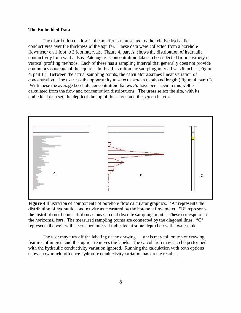
The Embedded Data

The distribution of flow in the aquifer is represented by the relative hydraulicconductivies over the thickness of the aquifer. These data were collected from a boreholeflowmeter on 1 foot to 3 foot intervals. Figure 4, part A, shows the distribution of hydraulicconductivity for a well at East Patchogue. Concentration data can be collected from a variety ofvertical profiling methods. Each of these has a sampling interval that generally does not providecontinuous coverage of the aqufier. In this illustration the sampling interval was 6 inches (Figure4, part B). Between the actual sampling points, the calculator assumes linear variation ofconcentration. The user has the opportunity to select a screen depth and length (Figure 4, part C). With these the average borehole concentration that would have been seen in this well iscalculated from the flow and concentration distributions. The users select the site, with itsembedded data set, the depth of the top of the screen and the screen length.

Figure 4 Illustration of components of borehole flow calculator graphics. “A” represents thedistribution of hydraulic conductivity as measured by the borehole flow meter. “B” representsthe distribution of concentration as measured at discrete sampling points. These correspond tothe horizontal bars. The measured sampling points are connected by the diagonal lines. “C”represents the well with a screened interval indicated at some depth below the watertable.

The user may turn off the labeling of the drawing. Labels may fall on top of drawingfeatures of interest and this option removes the labels. The calculation may also be performedwith the hydraulic conductivity variation ignored. Running the calculation with both optionsshows how much influence hydraulic conductivity variation has on the results.

9

Calculation Method

The average borehole concentration is calculated by averaging the mass flux from eachlayer in the profile. Each increment of mass flux is determined from

(1)

where )Ji is the increment of mass flux for depth increment i, Kri is the relative hydraulicconductivity for the increment, c(z) is the depth varying concentration over the increment, and zi-and zi+ are the depths of the top and bottom of depth increment ), respectively. The integrationis completed by assuming that c(z) follows a linear function between the measurement intervals.

Example Results

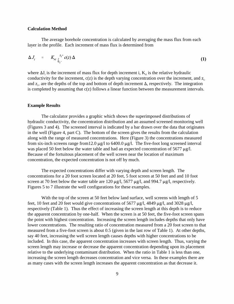
The calculator provides a graphic which shows the superimposed distributions ofhydraulic conductivity, the concentration distribution and an assumed screened monitoring well(Figures 3 and 4). The screened interval is indicated by a bar drawn over the data that originatesin the well (Figure 4, part C). The bottom of the screen gives the results from the calculationalong with the range of measured concentrations. Here (Figure 3) the concentrations measuredfrom six-inch screens range from12.0 :g/l to 6400.0 :g/l. The five-foot long screened intervalwas placed 50 feet below the water table and had an expected concentration of 5677 :g/l. Because of the fortuitous placement of the well screen near the location of maximumconcentration, the expected concentration is not off by much.

The expected concentrations differ with varying depth and screen length. Theconcentrations for a 20 foot screen located at 20 feet, 5 foot screen at 50 feet and and 10 footscreen at 70 feet below the water table are 120 :g/l, 5677 :g/l, and 994.7 :g/l, respectively. Figures 5 to 7 illustrate the well configurations for these examples.

With the top of the screen at 50 feet below land surface, well screens with length of 5feet, 10 feet and 20 feet would give concentrations of 5677 :g/l, 4849 :g/l, and 3028 :g/l,respectively (Table 1). Thus the effect of increasing the screen length at this depth is to reducethe apparent concentration by one-half. When the screen is at 50 feet, the five-foot screen spansthe point with highest concentration. Increasing the screen length includes depths that only havelower concentrations. The resulting ratio of concentration measured from a 20 foot screen to thatmeasured from a five-foot screen is about 0.5 (given in the last row of Table 1). At other depths,say 40 feet, increasing the well screen length causes depths with higher concentrations to beincluded. In this case, the apparent concentration increases with screen length. Thus, varying thescreen length may increase or decrease the apparent concentration depending upon its placementrelative to the underlying contaminant distribution. When the ratio in Table 1 is less than one,increasing the screen length decreases concentration and vice versa. In these examples there areas many cases with the screen length increases the apparent concentration as that decrease it.

10

ScreenLength(feet)

Depth of Well Screen Top

20feet

30feet

40feet

50feet

60feet

70feet

80feet

90feet

5 0 280 1054 5677 877 1155 561 80

10 0 210 1805 4849 1054 995 476 62

20 120 761 3524 3028 1130 743 316 37

Concentration ratio (20 ft screen:5 ft screen)

– – 2.7 3.3 0.53 1.3 0.64 0.56 0.46

Table 1 Effects of well screen length on concentrations given in :g/L observed wellsscreened from 20 feet to 90 feet below the land surface at East Patchogue, New York.

Figure 5 Estimated borehole concentrationof 120 :g/L for a twenty-foot long wellscreen located 20 feet below the landsurface.

Figure 6 Estimated borehole concentration of 5677 :g/L for a five-foot well screenlocated 50 feet below the land surface.

11

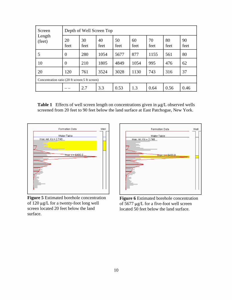
Figure 7 Estimated borehole concentrationof 995 :g/L for a ten-foot long well screenplaced 70 feet below the land surface.

3) Observation of Vertical Gradients

Estimation of vertical gradient are one tool for assessing the possibility of vertical flows.Water levels in nested well clusters (wells located closely together) indicate upward ordownward flowin aquifers or flow between adjacent geologic units. Flow is governed by Darcy'sLaw:

(2)

where q is the Darcy flux (volume of water per unit area per unit time) [L/T] and K is thehydraulic conductivity [L/T]. The change of head (roughly water level) divided by the distancedetermines the magnitude and direction of flow. Figure 8 shows the relative relationshipsbetween two wells. With respect to each other, one is shallow and the other deep. The figurealso indicates the important dimensions: depth to water (dw), depth to the top of the screen (d)and the screen length(s).

12

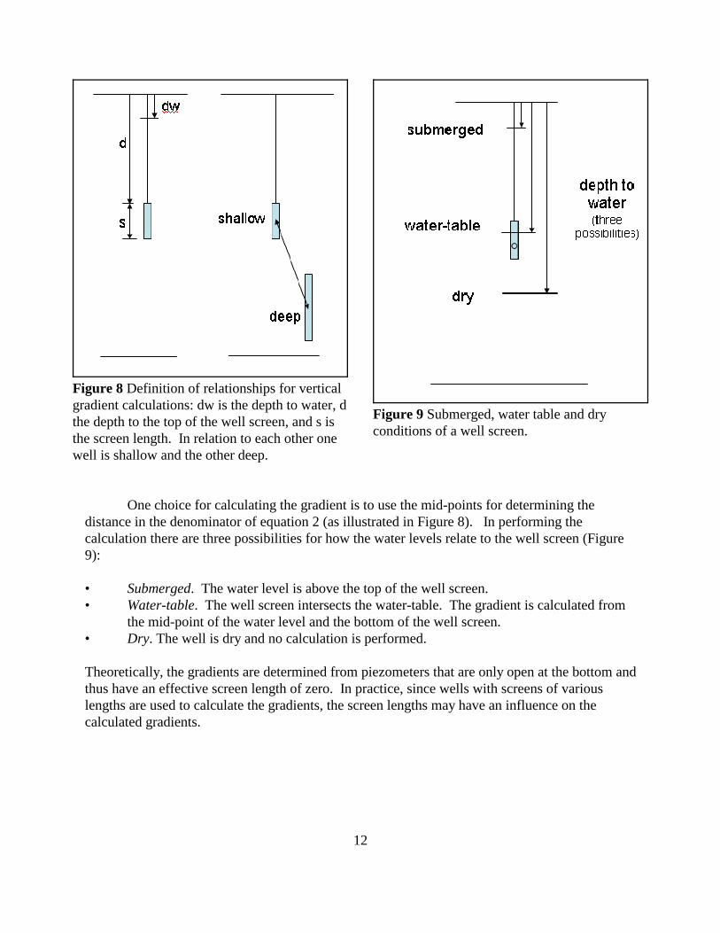
Figure 8 Definition of relationships for verticalgradient calculations: dw is the depth to water, dthe depth to the top of the well screen, and s isthe screen length. In relation to each other onewell is shallow and the other deep.

Figure 9 Submerged, water table and dryconditions of a well screen.

One choice for calculating the gradient is to use the mid-points for determining thedistance in the denominator of equation 2 (as illustrated in Figure 8). In performing thecalculation there are three possibilities for how the water levels relate to the well screen (Figure9):

• Submerged. The water level is above the top of the well screen.• Water-table. The well screen intersects the water-table. The gradient is calculated from

the mid-point of the water level and the bottom of the well screen.• Dry. The well is dry and no calculation is performed.

Theoretically, the gradients are determined from piezometers that are only open at the bottom andthus have an effective screen length of zero. In practice, since wells with screens of variouslengths are used to calculate the gradients, the screen lengths may have an influence on thecalculated gradients.

13

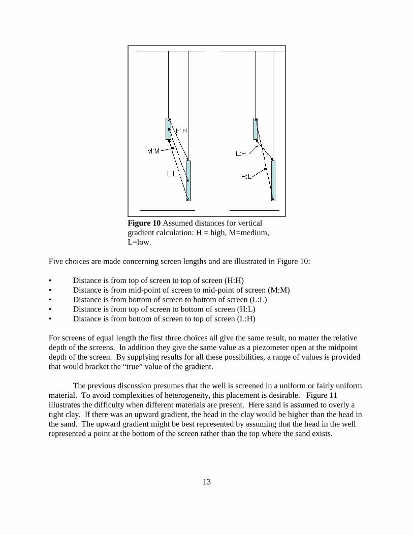
Figure 10 Assumed distances for verticalgradient calculation: H = high, M=medium,L=low.

Five choices are made concerning screen lengths and are illustrated in Figure 10:

• Distance is from top of screen to top of screen (H:H)• Distance is from mid-point of screen to mid-point of screen (M:M)• Distance is from bottom of screen to bottom of screen (L:L)• Distance is from top of screen to bottom of screen (H:L)• Distance is from bottom of screen to top of screen (L:H)

For screens of equal length the first three choices all give the same result, no matter the relativedepth of the screens. In addition they give the same value as a piezometer open at the midpointdepth of the screen. By supplying results for all these possibilities, a range of values is providedthat would bracket the “true” value of the gradient.

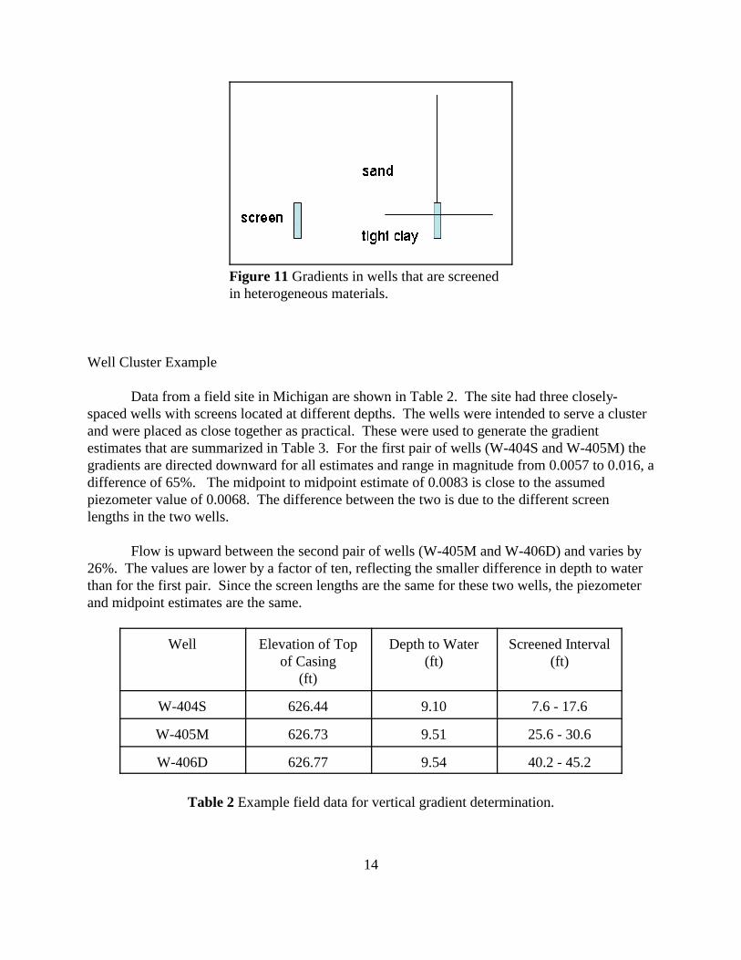
The previous discussion presumes that the well is screened in a uniform or fairly uniformmaterial. To avoid complexities of heterogeneity, this placement is desirable. Figure 11illustrates the difficulty when different materials are present. Here sand is assumed to overly atight clay. If there was an upward gradient, the head in the clay would be higher than the head inthe sand. The upward gradient might be best represented by assuming that the head in the wellrepresented a point at the bottom of the screen rather than the top where the sand exists.

14

Figure 11 Gradients in wells that are screenedin heterogeneous materials.

Well Cluster Example

Data from a field site in Michigan are shown in Table 2. The site had three closely-spaced wells with screens located at different depths. The wells were intended to serve a clusterand were placed as close together as practical. These were used to generate the gradientestimates that are summarized in Table 3. For the first pair of wells (W-404S and W-405M) thegradients are directed downward for all estimates and range in magnitude from 0.0057 to 0.016, adifference of 65%. The midpoint to midpoint estimate of 0.0083 is close to the assumedpiezometer value of 0.0068. The difference between the two is due to the different screenlengths in the two wells.

Flow is upward between the second pair of wells (W-405M and W-406D) and varies by26%. The values are lower by a factor of ten, reflecting the smaller difference in depth to waterthan for the first pair. Since the screen lengths are the same for these two wells, the piezometerand midpoint estimates are the same.

Well Elevation of Topof Casing

(ft)

Depth to Water(ft)

Screened Interval(ft)

W-404S 626.44 9.10 7.6 - 17.6

W-405M 626.73 9.51 25.6 - 30.6

W-406D 626.77 9.54 40.2 - 45.2

Table 2 Example field data for vertical gradient determination.

6The gradient was calculated from 22 in/yr (0.005 ft/d) divided by 400 ft/d.

15

Wells Estimated Gradients

direction Smallest Midpoint toMidpoint

Piezometer High Value

W-404S &W-405M

down 0.0057 0.0083 0.0068 0.016

W-405M &W-406D

up 0.00051 0.00069 0.00069 0.0010

Table 3 Example gradient estimates indicating the smallest, midpoint to midpoint, highestand the value for a piezometer.

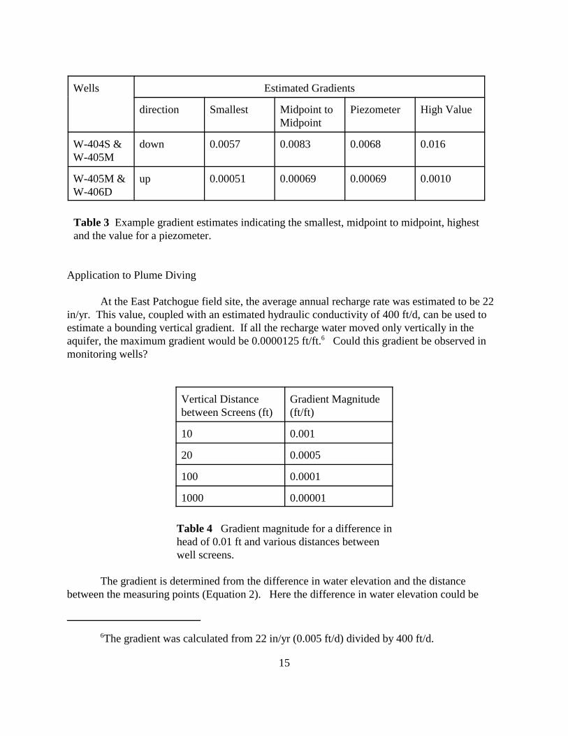
Application to Plume Diving

At the East Patchogue field site, the average annual recharge rate was estimated to be 22in/yr. This value, coupled with an estimated hydraulic conductivity of 400 ft/d, can be used toestimate a bounding vertical gradient. If all the recharge water moved only vertically in theaquifer, the maximum gradient would be 0.0000125 ft/ft.6 Could this gradient be observed inmonitoring wells?

Vertical Distancebetween Screens (ft)

Gradient Magnitude(ft/ft)

10 0.001

20 0.0005

100 0.0001

1000 0.00001

Table 4 Gradient magnitude for a difference inhead of 0.01 ft and various distances betweenwell screens.

The gradient is determined from the difference in water elevation and the distancebetween the measuring points (Equation 2). Here the difference in water elevation could be

16

assumed to be the smallest measurable difference: 0.01 feet. By selecting various distancesbetween the screens, Table 4 shows that a difference of 1000 ft in screen position is necessary todetect a vertical gradient of 0.00001. Thus it is unlikely that recharge-driven plume diving wouldbe detected by water level differences in monitoring wells.

Recharge-Driven Plume Diving Calculation

The prospects for plume diving should be considered when placing wells at all sites. Thefirst consideration should be indications of dipping strata from well logs. These can control thedistribution of contaminants down gradient from the source. Recharge can also cause plumediving. The calculator shows the effect due to recharge only. The implication of the results arethat for some aquifers the recharge of clean water to the aquifer can push the plume deeper intothe aquifer.

The plume diving calculator was designed to be used as a tool for site assessment byfollowing these steps:

• Estimate the required parameters for the each segment of the flow system:• Up and down gradient heads,• Aquifer hydraulic conductivity, and the

• Recharge rate.• Run the calculator for the proposed well location,• Check the plume depth at the location, and• Locate the well screen in appropriate vertical intervals.

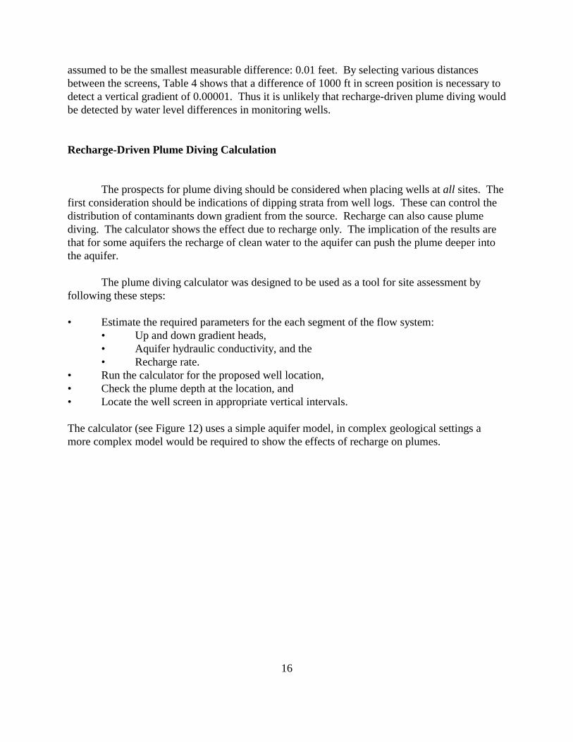
The calculator (see Figure 12) uses a simple aquifer model, in complex geological settings amore complex model would be required to show the effects of recharge on plumes.

17

Figure 12 Input and output screen for the plume diving calculator.

Theory

The recharge calculator is based upon two solutions of the one-dimensional Dupuitequation for flow in unconfined aquifers. These solutions are combined to determine theposition of the phreatic surface (water table) and a streamline originating at the water table, thegradient, ground water fluxes and travel times for sorbing contaminants. The methods used forperforming these calculations are given in Appendix 3.

18

East Patchogue Example

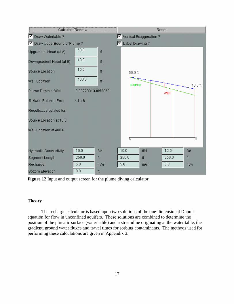
This method was developed for application to the MTBE and benzene plumes at EastPatchogue, New York. At this site the plume appeared to drop when it moved below a sand andgravel mining operation. Data collected from a borehole flow meter on the variation of hydraulicconductivity with depth showed no direct connection between contaminant concentrations andhydraulic conductivity. From this it was concluded that statigraphy did not cause the diving ofthe plume. The plume diving calculation was developed to assess the contribution of recharge tothe dropping of the plume. The results of the calculations are shown in Figure 13. The linelabeled “A” represents the water table, which was calibrated to observed elevations. The linelabeled “B” was determined from the plume diving calculator, using the calibrated water levels,hydraulic conductivity calibrated from a transport model (Weaver, 1996), and assumptionsconcerning the recharge. Most importantly, the average recharge on Long Island is estimated tobe 22 in/year by the USGS. In the area of the sand and gravel pit (Segment 2 on Figure 13) theentire annual rainfall of 44 in/year was assumed to recharge the aquifer. The combination ofthese inputs was sufficient to produce line “B” which is the best estimate of the upper bound ofthe contaminant plume.

Although the calculation reproduces the field behavior, the best use of the calculator iswhere vertical data are not yet available. Using recharge estimates and land use characteristics anestimate of plume diving can be made. Sampling can then be made at appropriate elevations. Since there are many factors that influence the accuracy of the method, not the least being theassumption of one-dimensional flow, the calculator predictions are not intended to give the “lastword” on plume diving. Rather the calculator results should guide placement of well screens.

19

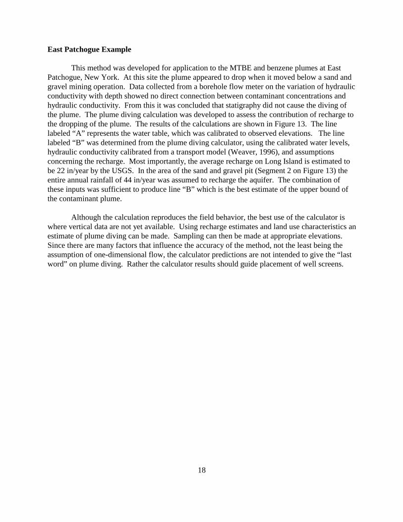
Figure 13 Example plume diving calculation for the East Patchogue site. “A”represents the watertable which was calibrated to the field data. “B” represents anuncalibrated prediction of the top of the plume determined from the plume divingcalculator.

Required Input

The plume diving calculator requires input to 1) Define the hydraulics of the flow systemand 2) Contaminant source and observation well location. The single screen of the plume divinginterface is used for parameter entry, reporting of results and graphing the solution. Thefollowing drawings show an exploded view of the interface.

Flow System Hydraulics

The aquifer is divided into segments and for each the hydraulic conductivity, rechargerate, and length must be specified (Figure 14). A uniform aquifer can be simulated by using thesame parameter values for each segment.

Figure 14 Plume Diving calculator hydraulic and hydrologic property entry.

20

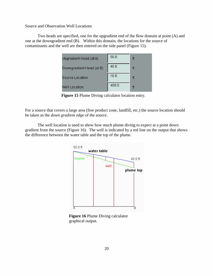
Source and Observation Well Locations

Two heads are specified, one for the upgradient end of the flow domain at point (A) andone at the downgradient end (B). Within this domain, the locations for the source ofcontaminants and the well are then entered on the side panel (Figure 15).

Figure 15 Plume Diving calculator location entry.

For a source that covers a large area (free product zone, landfill, etc.) the source location shouldbe taken as the down gradient edge of the source.

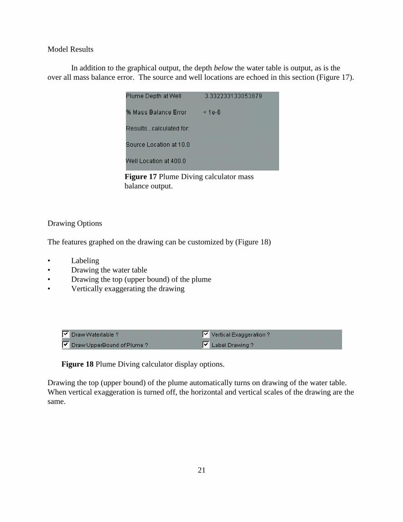
The well location is used to show how much plume diving to expect at a point downgradient from the source (Figure 16). The well is indicated by a red line on the output that showsthe difference between the water table and the top of the plume.

Figure 16 Plume Diving calculatorgraphical output.

21

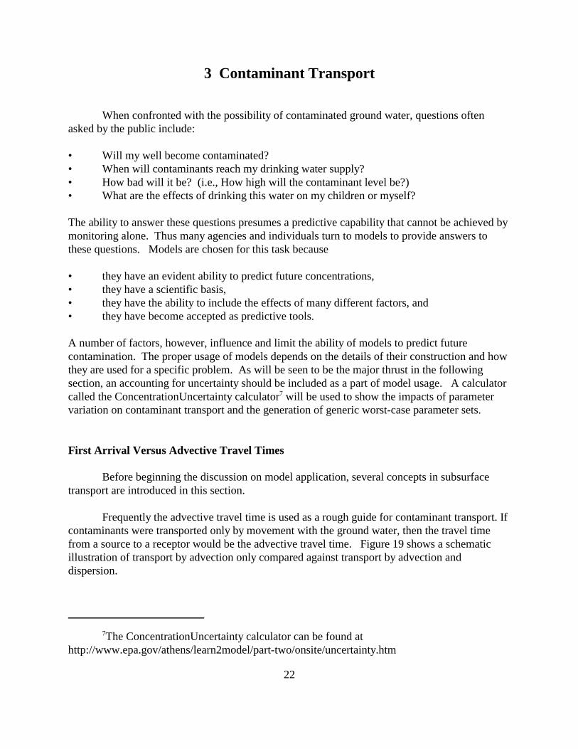
Model Results

In addition to the graphical output, the depth below the water table is output, as is theover all mass balance error. The source and well locations are echoed in this section (Figure 17).

Figure 17 Plume Diving calculator massbalance output.

Drawing Options

The features graphed on the drawing can be customized by (Figure 18)

• Labeling• Drawing the water table• Drawing the top (upper bound) of the plume• Vertically exaggerating the drawing

Figure 18 Plume Diving calculator display options.

Drawing the top (upper bound) of the plume automatically turns on drawing of the water table.When vertical exaggeration is turned off, the horizontal and vertical scales of the drawing are thesame.

7The ConcentrationUncertainty calculator can be found athttp://www.epa.gov/athens/learn2model/part-two/onsite/uncertainty.htm

22

3 Contaminant Transport

When confronted with the possibility of contaminated ground water, questions oftenasked by the public include:

• Will my well become contaminated?• When will contaminants reach my drinking water supply?• How bad will it be? (i.e., How high will the contaminant level be?)• What are the effects of drinking this water on my children or myself?

The ability to answer these questions presumes a predictive capability that cannot be achieved bymonitoring alone. Thus many agencies and individuals turn to models to provide answers tothese questions. Models are chosen for this task because

• they have an evident ability to predict future concentrations,• they have a scientific basis, • they have the ability to include the effects of many different factors, and• they have become accepted as predictive tools.

A number of factors, however, influence and limit the ability of models to predict futurecontamination. The proper usage of models depends on the details of their construction and howthey are used for a specific problem. As will be seen to be the major thrust in the followingsection, an accounting for uncertainty should be included as a part of model usage. A calculatorcalled the ConcentrationUncertainty calculator7 will be used to show the impacts of parametervariation on contaminant transport and the generation of generic worst-case parameter sets.

First Arrival Versus Advective Travel Times

Before beginning the discussion on model application, several concepts in subsurfacetransport are introduced in this section.

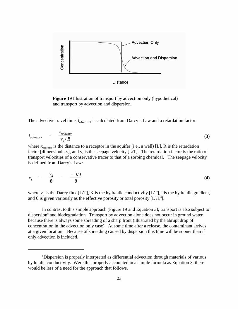
Frequently the advective travel time is used as a rough guide for contaminant transport. Ifcontaminants were transported only by movement with the ground water, then the travel timefrom a source to a receptor would be the advective travel time. Figure 19 shows a schematicillustration of transport by advection only compared against transport by advection anddispersion.

8Dispersion is properly interpreted as differential advection through materials of varioushydraulic conductivity. Were this properly accounted in a simple formula as Equation 3, therewould be less of a need for the approach that follows.

23

Figure 19 Illustration of transport by advection only (hypothetical)and transport by advection and dispersion.

The advective travel time, tadvective, is calculated from Darcy’s Law and a retardation factor:

(3)

where xreceptor is the distance to a receptor in the aquifer (i.e., a well) [L], R is the retardationfactor [dimensionless], and vs is the seepage velocity [L/T]. The retardation factor is the ratio oftransport velocities of a conservative tracer to that of a sorbing chemical. The seepage velocityis defined from Darcy’s Law:

(4)

where vd is the Darcy flux [L/T], K is the hydraulic conductivity [L/T], i is the hydraulic gradient,and 2 is given variously as the effective porosity or total porosity [L3/L3].

In contrast to this simple approach (Figure 19 and Equation 3), transport is also subject todispersion8 and biodegradation. Transport by advection alone does not occur in ground waterbecause there is always some spreading of a sharp front (illustrated by the abrupt drop ofconcentration in the advection only case). At some time after a release, the contaminant arrivesat a given location. Because of spreading caused by dispersion this time will be sooner than ifonly advection is included.

24

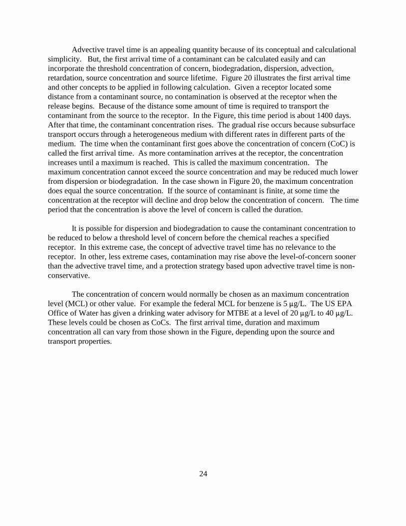
Advective travel time is an appealing quantity because of its conceptual and calculationalsimplicity. But, the first arrival time of a contaminant can be calculated easily and canincorporate the threshold concentration of concern, biodegradation, dispersion, advection,retardation, source concentration and source lifetime. Figure 20 illustrates the first arrival timeand other concepts to be applied in following calculation. Given a receptor located somedistance from a contaminant source, no contamination is observed at the receptor when therelease begins. Because of the distance some amount of time is required to transport thecontaminant from the source to the receptor. In the Figure, this time period is about 1400 days. After that time, the contaminant concentration rises. The gradual rise occurs because subsurfacetransport occurs through a heterogeneous medium with different rates in different parts of themedium. The time when the contaminant first goes above the concentration of concern (CoC) iscalled the first arrival time. As more contamination arrives at the receptor, the concentrationincreases until a maximum is reached. This is called the maximum concentration. Themaximum concentration cannot exceed the source concentration and may be reduced much lowerfrom dispersion or biodegradation. In the case shown in Figure 20, the maximum concentrationdoes equal the source concentration. If the source of contaminant is finite, at some time theconcentration at the receptor will decline and drop below the concentration of concern. The timeperiod that the concentration is above the level of concern is called the duration.

It is possible for dispersion and biodegradation to cause the contaminant concentration tobe reduced to below a threshold level of concern before the chemical reaches a specifiedreceptor. In this extreme case, the concept of advective travel time has no relevance to thereceptor. In other, less extreme cases, contamination may rise above the level-of-concern soonerthan the advective travel time, and a protection strategy based upon advective travel time is non-conservative.

The concentration of concern would normally be chosen as an maximum concentrationlevel (MCL) or other value. For example the federal MCL for benzene is 5 :g/L. The US EPAOffice of Water has given a drinking water advisory for MTBE at a level of 20 :g/L to 40 :g/L. These levels could be chosen as CoCs. The first arrival time, duration and maximumconcentration all can vary from those shown in the Figure, depending upon the source andtransport properties.

25

Figure 20 Illustration showing the relationship between the first arrivaltime, maximum concentration and duration of contamination. The firstarrival time and duration are determined relative to a given thresholdconcentration, that is usually a maximum contaminant level or otherconcentration of concern.

26

Uncertainty Range Determination

Models are commonly viewed as useful tools for understanding contaminant transport(Oreskes et al., 1994) and determining future risk (ASTM, 1995). The degree of predictivecapability of subsurface transport models has, in fact, not been established (e.g., Miller andGray, 2002, Eggleston and Rojstaczer, 2000). Given that the values of all the parameters(hydraulic conductivity, dispersivity, retardation factor, biodegradation rate constant) and theforcing function (source concentration and source duration) were known, and that theassumptions behind the model were exactly met, the model equations (Equation 24) could besolved for the required outputs. In the real world, however, the values are not exactly known andno aquifer would meet the required assumption of homogeneity. At leaking undergroundstorage tank (LUST) sites, it would typically be expected that hydraulic conductivities would bemeasured through slug tests and the other input parameters not measured. The sourceconcentration and duration would be unknown. Dispersivity, since it represents unaccountedheterogeneity, is clearly not a fundamental parameter and is best viewed as a fitting parameter:thus its appropriate value is also unknown.

Models are more likely to provide a framework for understanding transport than forpredicting future exposure and risk. Commonly, models are calibrated to field data todemonstrate their ability to reproduce contaminant behavior at a site. This process implies adegree of correctness in understanding and provides the first step toward demonstration ofpredictive ability. For screening sites or where rapid response is required, sufficient data may notbe collected for calibrating a model. How then should models be used in situations where theycan not or will not be calibrated? What are the plausible ranges of output given uncertainty ininputs? Can worst case parameter sets be selected that always provide a bound on plausibleoutcomes?

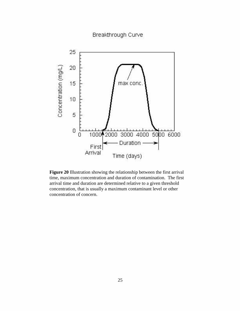
Figure 21 shows a conceptual relationship between uncertainty and data availability. With small amounts of either measured input data or calibration data, the resulting modeluncertainty is high. Models may still be useful in these cases, but their uncertainty should bequantified so that their results are not taken falsely as inerrant.

Figure 21 Relationship of uncertainty to model dataavailability.

27

Approach

Several approaches to uncertainty analysis have been developed. Generally these requireknowledge of parameter values and their statistical distributions including correlations betweenindividual parameters. Here site investigations are not sufficiently detailed to determine valuesfor some of the parameters, let alone their statistical distributions and correlations. A briefaccounting of the model inputs is given as follows: Porosity and dispersivity are essentiallynever determined on a site-specific basis, despite their importance in determining modeloutcomes. Biodegradation rate constants may be estimated from simple techniques (Buscheckand Alacantar, 1995), but these require adherence to a suite of restrictive assumptions that limitsthe results by the same considerations that we are attempting to address in this work. Parametersmeasured in the field are subject to uncertainty because of spatial variability (hydraulicconductivity and fraction organic carbon) or temporal fluctuations (gradients). The forcingparameters of the model, initial concentration and duration, are rarely known, becausecontamination is normally discovered years after a release occurs.

There is a similar lack of knowledge of statistical distributions of the inputs. A widely-used alternative is to assume knowledge of the statistical properties by using scientific literaturevalues as substitutes. These approaches allow assignment of probabilities to the variousoutcomes, but suffers from obvious lack of site-specificity. Where results depend strongly onassumed distributions, it is not possible to determine how much error is introduced into theresults from the distributions. Alternatively, if it is assumed only that plausible ranges of inputparameters are known, similar outcomes can be determined, but probabilities cannot be assigned. Because of lack of knowledge of the underlying probability distributions, a method based onranges of inputs was developed.

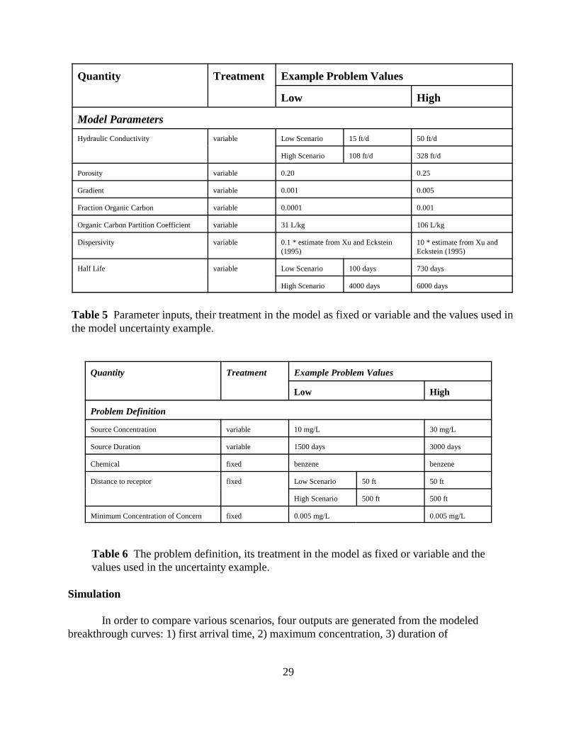
Nine parameters of the one-dimensional model (Equation 24) are assumed to be variable. Tables 5 and 6 list parameters and their treatment in the model. All seven parameters of themodel were allowed to be variable, as were the concentration and duration of the source. Thechemical, distance to receptor, and minimum concentration of concern are taken as fixed for agiven analysis. With this selection of inputs there are two values each for nine parameters: theminimum value and the maximum value. This leads to a total of 29 or 512 unique combinationsof parameters. This calculation highlights an assumption of this method: That each parametervalue is equally likely and can occur in combination with each other parameter value. In otherwords that each parameter is uniformly distributed and uncorrelated. The large number ofparameter combinations is the reason to seek models that execute rapidly. Hence the interest inthe one-dimensional model.

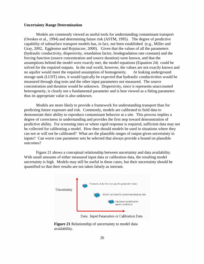
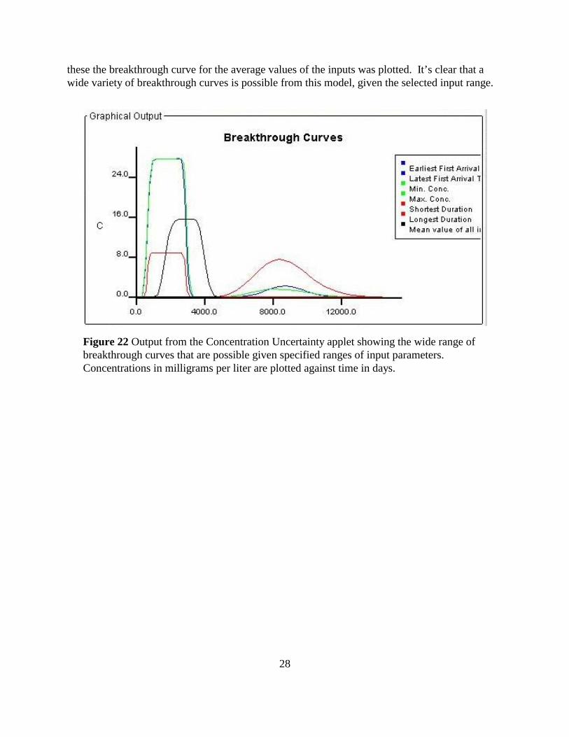
Figure 22 shows an example output where breakthrough curves representing variousbreakthrough curves have been plotted. These have been selected from the 512 outputs of themodel to represent the significant outputs of the model: earliest and latest first arrival times,minimum and maximum peak concentration, and the longest and shortest duration. Along with

28

these the breakthrough curve for the average values of the inputs was plotted. It’s clear that awide variety of breakthrough curves is possible from this model, given the selected input range.

Figure 22 Output from the Concentration Uncertainty applet showing the wide range ofbreakthrough curves that are possible given specified ranges of input parameters. Concentrations in milligrams per liter are plotted against time in days.

29

Quantity Treatment Example Problem Values

Low High

Model ParametersHydraulic Conductivity variable Low Scenario 15 ft/d 50 ft/d

High Scenario 108 ft/d 328 ft/d

Porosity variable 0.20 0.25

Gradient variable 0.001 0.005

Fraction Organic Carbon variable 0.0001 0.001

Organic Carbon Partition Coefficient variable 31 L/kg 106 L/kg

Dispersivity variable 0.1 * estimate from Xu and Eckstein(1995)

10 * estimate from Xu andEckstein (1995)

Half Life variable Low Scenario 100 days 730 days

High Scenario 4000 days 6000 days

Table 5 Parameter inputs, their treatment in the model as fixed or variable and the values used inthe model uncertainty example.

Quantity Treatment Example Problem Values

Low High

Problem Definition

Source Concentration variable 10 mg/L 30 mg/L

Source Duration variable 1500 days 3000 days

Chemical fixed benzene benzene

Distance to receptor fixed Low Scenario 50 ft 50 ft

High Scenario 500 ft 500 ft

Minimum Concentration of Concern fixed 0.005 mg/L 0.005 mg/L

Table 6 The problem definition, its treatment in the model as fixed or variable and thevalues used in the uncertainty example.

Simulation

In order to compare various scenarios, four outputs are generated from the modeledbreakthrough curves: 1) first arrival time, 2) maximum concentration, 3) duration of

30

contamination, and 4) risk factor. This first three of these are illustrated in Figure 22. Cancerrisk is normally determined from an expression of the form (US EPA, 1989)

(5)

where I is the intake in mg/kg-day, SF is the cancer slope factor (kg-day/mg), CW is theconcentration in water (mg/L), ED is the exposure duration (days), EF is the exposure frequency(days/year), IR is the injestion rate (liters/day), BW is the body weight (kg), and AT is theaveraging time (years). Since concentrations on the breakthrough curve change with time, theeffect of the transient in concentration is included in the risk equation by using the substitution:

(6)

where CW(t) are the modeled concentrations, to is the contaminant first arrival time, ta is the lasttime that the concentration is above the threshold. Thus the integral of concentration versus timegives a measure of relative risk. The model accumulates results and determines the best andworse cases for each of the four chosen breakthrough curve outputs.

In addition to variable parameters, four scenarios were created to simulate a variety ofconditions and determine if the model behavior was similar despite variation in parameter values. Two ranges each of hydraulic conductivity and half life were selected (Table 6). These variableswere chosen to vary because they have a direct effect on model outputs: Hydraulic conductivityaffects advective transport rates and thus the arrival times and duration of contamination, and thehalf life impacts maximum concentration. Risk is affected by both concentration and duration. The scenarios are generally comparable with each other with the exception that the receptor iscloser to the source in the low conductivity scenario. This selection was made so that therewould be complete breakthrough curves for all combinations of parameters in each scenario.

Results

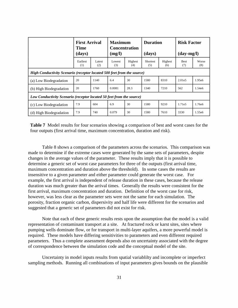
Table 7 shows the extreme cases for four problem scenarios (see Table 5): High and lowconductivity aquifers, and high and low biodegradation rates. These results show the magnitudeof possible outcomes given the range of inputs used. The high and low conductivity scenarioshave a different distance to the receptor (500 ft versus 50 ft), so the first arrival time results arenot directly comparable. In going 10 times further in the high conductivity scenario the arrivaltime is approximately 2.5 times greater than the low conductivity scenario (20 days/7.9 days),indicating proportionately earlier first arrival in the high conductivity scenario. The minimumdurations are in part determined by the source duration (which at a minimum is 1500 days). With high biodegradation rates the minimum concentrations can be greatly reduced (comparerow a and b and row c and d in column 3) in either scenario.

31

First ArrivalTime(days)

MaximumConcentration(mg/l)

Duration

(days)

Risk Factor

(day-mg/l)Earliest

(1)Latest

(2)Lowest

(3)Highest

(4)Shortest

(5)Highest

(6)Best(7)

Worse(8)

High Conductivity Scenario (receptor located 500 feet from the source)

(a) Low Biodegradation 20 1140 6.4 30 1580 8310 2.01e5 1.95e6

(b) High Biodegradation 20 1760 0.0081 28.3 1340 7210 562 1.54e6

Low Conductivity Scenario (receptor located 50 feet from the source)

(c) Low Biodegradation 7.9 604 6.9 30 1580 9210 1.71e5 1.76e6

(d) High Biodegradation 7.9 740 0.079 30 1580 7610 3330 1.55e6

Table 7 Model results for four scenarios showing a comparison of best and worst cases for thefour outputs (first arrival time, maximum concentration, duration and risk).

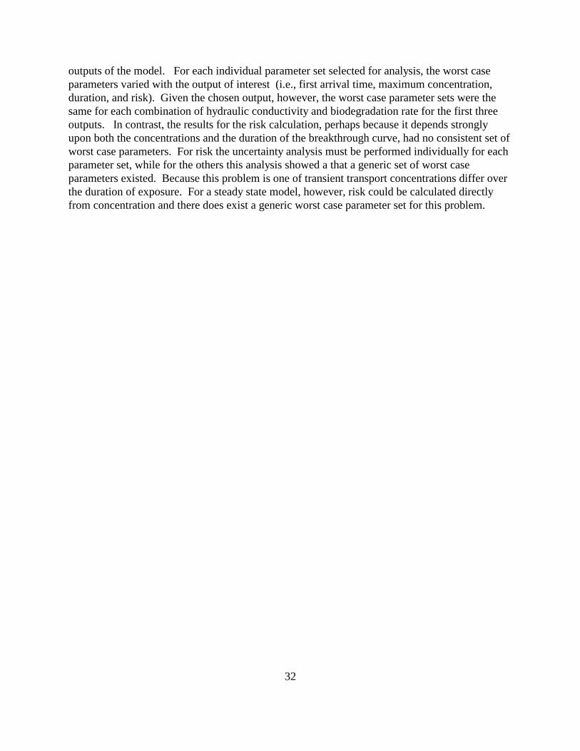
Table 8 shows a comparison of the parameters across the scenarios. This comparison wasmade to determine if the extreme cases were generated by the same sets of parameters, despitechanges in the average values of the parameter. These results imply that it is possible todetermine a generic set of worst case parameters for three of the outputs (first arrival time,maximum concentration and duration above the threshold). In some cases the results areinsensitive to a given parameter and either parameter could generate the worst case. Forexample, the first arrival is independent of release duration in these cases, because the releaseduration was much greater than the arrival times. Generally the results were consistent for thefirst arrival, maximum concentration and duration. Definition of the worst case for risk,however, was less clear as the parameter sets were not the same for each simulation. Theporosity, fraction organic carbon, dispersivity and half life were different for the scenarios andsuggested that a generic set of parameters did not exist for risk.

Note that each of these generic results rests upon the assumption that the model is a validrepresentation of contaminant transport at a site. At fractured rock or karst sites, sites wherepumping wells dominate flow, or for transport in multi-layer aquifers, a more powerful model isrequired. These models have differing sensitivities to parameters and even different requiredparameters. Thus a complete assessment depends also on uncertainty associated with the degreeof correspondence between the simulation code and the conceptual model of the site.

Uncertainty in model inputs results from spatial variablilty and incomplete or imperfectsampling methods. Running all combinations of input parameters gives bounds on the plausible

32

outputs of the model. For each individual parameter set selected for analysis, the worst caseparameters varied with the output of interest (i.e., first arrival time, maximum concentration,duration, and risk). Given the chosen output, however, the worst case parameter sets were thesame for each combination of hydraulic conductivity and biodegradation rate for the first threeoutputs. In contrast, the results for the risk calculation, perhaps because it depends stronglyupon both the concentrations and the duration of the breakthrough curve, had no consistent set ofworst case parameters. For risk the uncertainty analysis must be performed individually for eachparameter set, while for the others this analysis showed a that a generic set of worst caseparameters existed. Because this problem is one of transient transport concentrations differ overthe duration of exposure. For a steady state model, however, risk could be calculated directlyfrom concentration and there does exist a generic worst case parameter set for this problem.

33

Scenario

Hyd

raul

ic C

ondu

ctiv

ity

Poro

sity

Gra

dien

t

Frac

tion

orga

nic

carb

on Koc

Dis

pers

ivity

Hal

f Life

Sour

ce c

onc

Sour

ceD

urat

ion

Earliest First Arrival

Low Conductivity, Low Biodegradation H L H L L H E H E

Low Conductivity, High Biodegradation H L H L L H E H E

High Conductivity, Low Biodegradation H L H L L H E H E

High Conductivity, High Biodegradation H L H L L H E H E

Highest Maximum Concentration

Low Conductivity, Low Biodegradation H L H E E H H H E

Low Conductivity, High Biodegradation H L H E E H H H E

High Conductivity, Low Biodegradation H L H E E E H H E

High Conductivity, High Biodegradation H L H E E H H H E

Longest Duration

Low Conductivity, Low Biodegradation L H L H H H H H H

Low Conductivity, High Biodegradation L H L H H H H H H

High Conductivity, Low Biodegradation L H L H H H E H H

High Conductivity, High Biodegradation L H L H H H H H H

Highest Risk

Low Conductivity, Low Biodegradation L H H H H L L H H

Low Conductivity, High Biodegradation L H H H H L L H H

High Conductivity, Low Biodegradation L E L E E H E H H

High Conductivity, High Biodegradation L L L H L H H H H

H = high value, L = low value, E = either value

Table 8 Comparison of data sets giving the worst cases for each of four model outputs.

34

Concentration Uncertainty Model Input and Output

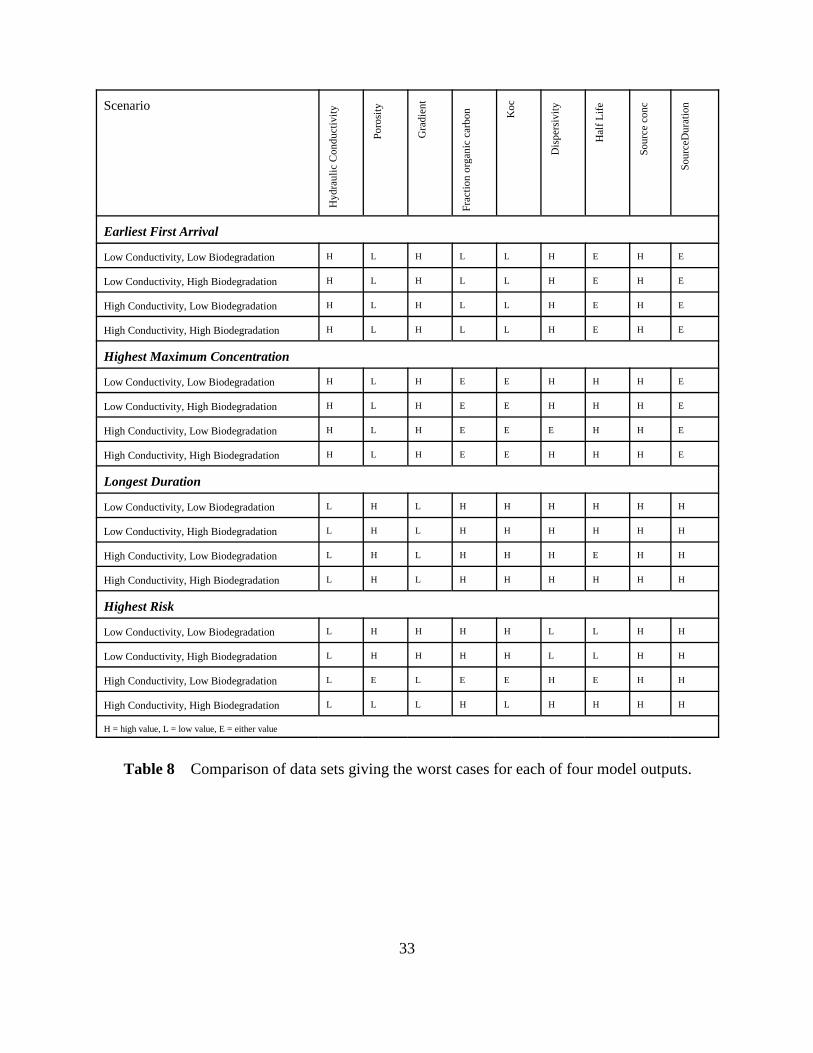
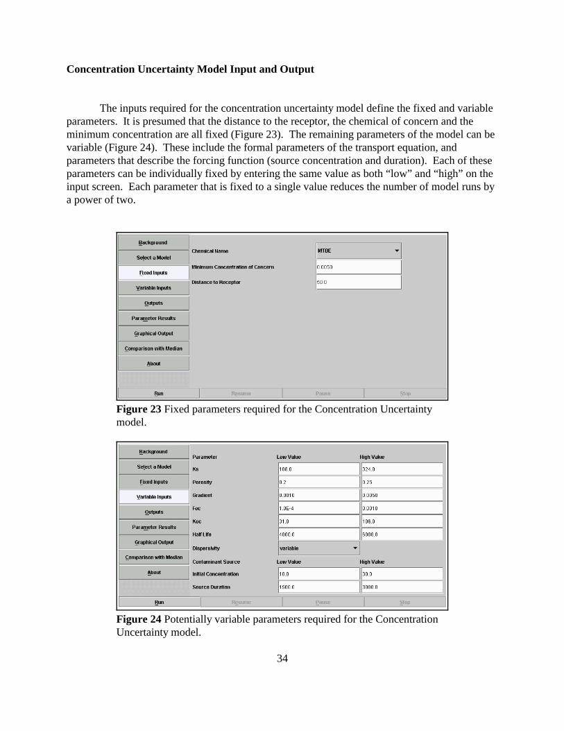
The inputs required for the concentration uncertainty model define the fixed and variableparameters. It is presumed that the distance to the receptor, the chemical of concern and theminimum concentration are all fixed (Figure 23). The remaining parameters of the model can bevariable (Figure 24). These include the formal parameters of the transport equation, andparameters that describe the forcing function (source concentration and duration). Each of theseparameters can be individually fixed by entering the same value as both “low” and “high” on theinput screen. Each parameter that is fixed to a single value reduces the number of model runs bya power of two.

Figure 23 Fixed parameters required for the Concentration Uncertaintymodel.

Figure 24 Potentially variable parameters required for the ConcentrationUncertainty model.

35

Model Outputs

The major outputs of the model are displayed on three output screens. The first of theoutput screens shows the values of all the key outputs of the model: first arrival time, maximumconcentration, duration above threshold concentration and the risk factor (Figure 25). These areeach show for the best and worst case. In addition to displaying the value of the parameter ofinterest, say the first arrival time, each line of output also shows the associated values of all otheroutputs.

If it could be determined that a generic set of best and worst case parameter existed, thenit would not be necessary to run an uncertainty analysis every time the model was run. Figure 26indicates which parameter (low or high value) resulted in each model outcome. From these it hasbeen shown that generic worst cases exist for some of the outputs. (See the example problemoutputs and discussion.)

Thirdly, the output breakthrough curves are plotted against the breakthrough curve for theaverage of all input values. These plots show the wide range of possible model outcomes (Figure27). The families of curves can be moved closer together by fixing values of variable inputparameters. Exploring which parameters could benefit from improved estimates can help focussite assessment activities.

Figure 25 Output from the Concentration Uncertainty model showing the extreme values foreach model output: first arrival, maximum concentration, duration above threshold and riskfactor.

36

Figure 26 Generic values (low or high) of parameter sets that generate extreme values of eachoutput of the model: first arrival time, maximum concentration, duration and risk factor.

Figure 27 Graphical presentation of Concentration Uncertainty modeloutput showing a comparison of the breakthrough curves for the extremesof each model output: first arrival time, maximum concentration, duration,and risk factor with the breakthrough curve for the average value of allinputs.

9http://www.epa.gov/athens/learn2model/part-two/onsite/retard.htm

37

4. Model Input Parameters

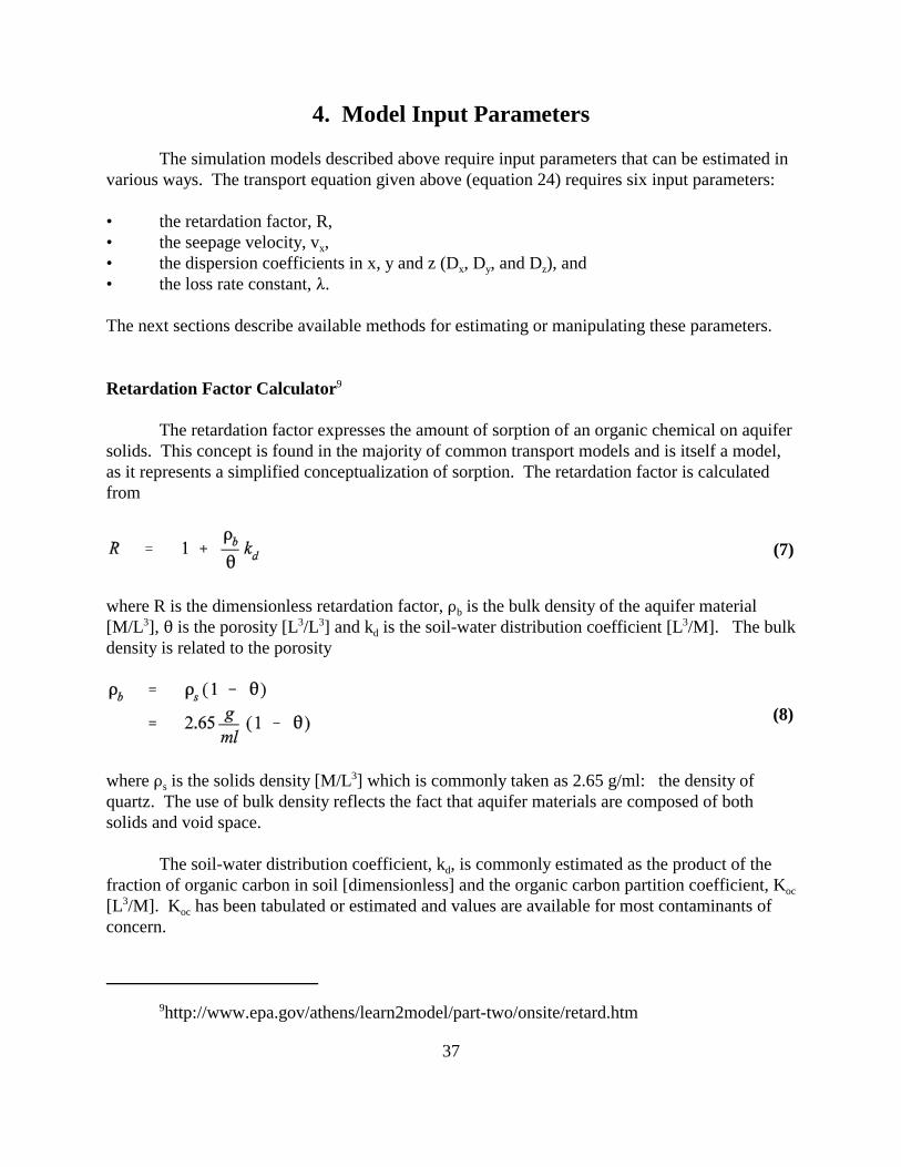
The simulation models described above require input parameters that can be estimated invarious ways. The transport equation given above (equation 24) requires six input parameters:

• the retardation factor, R,• the seepage velocity, vx,• the dispersion coefficients in x, y and z (Dx, Dy, and Dz), and• the loss rate constant, 8.

The next sections describe available methods for estimating or manipulating these parameters.

Retardation Factor Calculator9

The retardation factor expresses the amount of sorption of an organic chemical on aquifersolids. This concept is found in the majority of common transport models and is itself a model,as it represents a simplified conceptualization of sorption. The retardation factor is calculatedfrom

(7)

where R is the dimensionless retardation factor, Db is the bulk density of the aquifer material[M/L3], 2 is the porosity [L3/L3] and kd is the soil-water distribution coefficient [L3/M]. The bulkdensity is related to the porosity

(8)

where Ds is the solids density [M/L3] which is commonly taken as 2.65 g/ml: the density ofquartz. The use of bulk density reflects the fact that aquifer materials are composed of bothsolids and void space.

The soil-water distribution coefficient, kd, is commonly estimated as the product of thefraction of organic carbon in soil [dimensionless] and the organic carbon partition coefficient, Koc[L3/M]. Koc has been tabulated or estimated and values are available for most contaminants ofconcern.

38

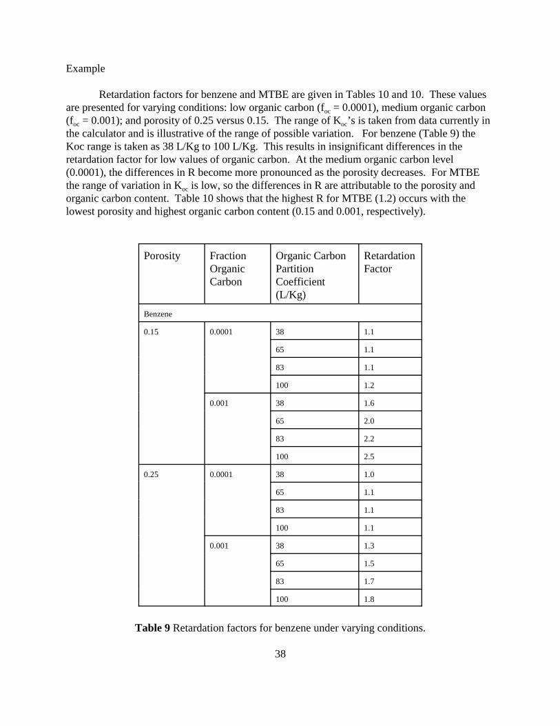
Example

Retardation factors for benzene and MTBE are given in Tables 10 and 10. These valuesare presented for varying conditions: low organic carbon (foc = 0.0001), medium organic carbon(foc = 0.001); and porosity of 0.25 versus 0.15. The range of Koc’s is taken from data currently inthe calculator and is illustrative of the range of possible variation. For benzene (Table 9) theKoc range is taken as 38 L/Kg to 100 L/Kg. This results in insignificant differences in theretardation factor for low values of organic carbon. At the medium organic carbon level(0.0001), the differences in R become more pronounced as the porosity decreases. For MTBEthe range of variation in Koc is low, so the differences in R are attributable to the porosity andorganic carbon content. Table 10 shows that the highest R for MTBE (1.2) occurs with thelowest porosity and highest organic carbon content (0.15 and 0.001, respectively).

Porosity FractionOrganicCarbon

Organic CarbonPartitionCoefficient(L/Kg)

RetardationFactor

Benzene

0.15 0.0001 38 1.1

65 1.1

83 1.1

100 1.2

0.001 38 1.6

65 2.0

83 2.2

100 2.5

0.25 0.0001 38 1.0

65 1.1

83 1.1

100 1.1

0.001 38 1.3

65 1.5

83 1.7

100 1.8

Table 9 Retardation factors for benzene under varying conditions.

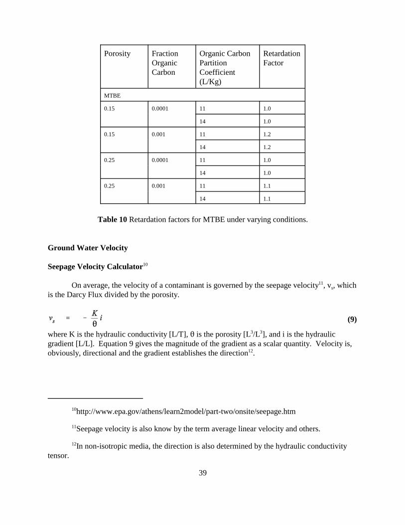
10http://www.epa.gov/athens/learn2model/part-two/onsite/seepage.htm

11Seepage velocity is also know by the term average linear velocity and others.

12In non-isotropic media, the direction is also determined by the hydraulic conductivitytensor.

39

Porosity FractionOrganicCarbon

Organic CarbonPartitionCoefficient(L/Kg)

RetardationFactor

MTBE

0.15 0.0001 11 1.0

14 1.0

0.15 0.001 11 1.2

14 1.2

0.25 0.0001 11 1.0

14 1.0

0.25 0.001 11 1.1

14 1.1

Table 10 Retardation factors for MTBE under varying conditions.

Ground Water Velocity

Seepage Velocity Calculator10

On average, the velocity of a contaminant is governed by the seepage velocity11, vs, whichis the Darcy Flux divided by the porosity.

(9)

where K is the hydraulic conductivity [L/T], 2 is the porosity [L3/L3], and i is the hydraulicgradient [L/L]. Equation 9 gives the magnitude of the gradient as a scalar quantity. Velocity is,obviously, directional and the gradient establishes the direction12.

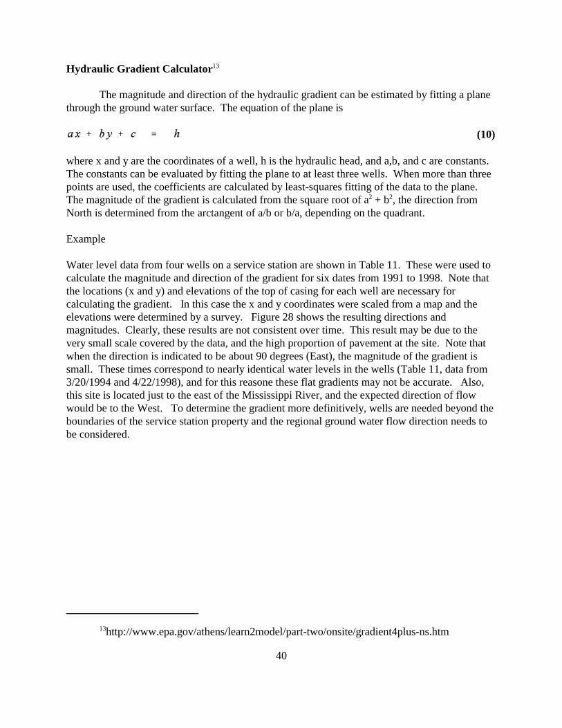
13http://www.epa.gov/athens/learn2model/part-two/onsite/gradient4plus-ns.htm

40

Hydraulic Gradient Calculator13

The magnitude and direction of the hydraulic gradient can be estimated by fitting a planethrough the ground water surface. The equation of the plane is

(10)

where x and y are the coordinates of a well, h is the hydraulic head, and a,b, and c are constants. The constants can be evaluated by fitting the plane to at least three wells. When more than threepoints are used, the coefficients are calculated by least-squares fitting of the data to the plane. The magnitude of the gradient is calculated from the square root of a2 + b2, the direction fromNorth is determined from the arctangent of a/b or b/a, depending on the quadrant.

Example

Water level data from four wells on a service station are shown in Table 11. These were used tocalculate the magnitude and direction of the gradient for six dates from 1991 to 1998. Note thatthe locations (x and y) and elevations of the top of casing for each well are necessary forcalculating the gradient. In this case the x and y coordinates were scaled from a map and theelevations were determined by a survey. Figure 28 shows the resulting directions andmagnitudes. Clearly, these results are not consistent over time. This result may be due to thevery small scale covered by the data, and the high proportion of pavement at the site. Note thatwhen the direction is indicated to be about 90 degrees (East), the magnitude of the gradient issmall. These times correspond to nearly identical water levels in the wells (Table 11, data from3/20/1994 and 4/22/1998), and for this reasone these flat gradients may not be accurate. Also,this site is located just to the east of the Mississippi River, and the expected direction of flowwould be to the West. To determine the gradient more definitively, wells are needed beyond theboundaries of the service station property and the regional ground water flow direction needs tobe considered.

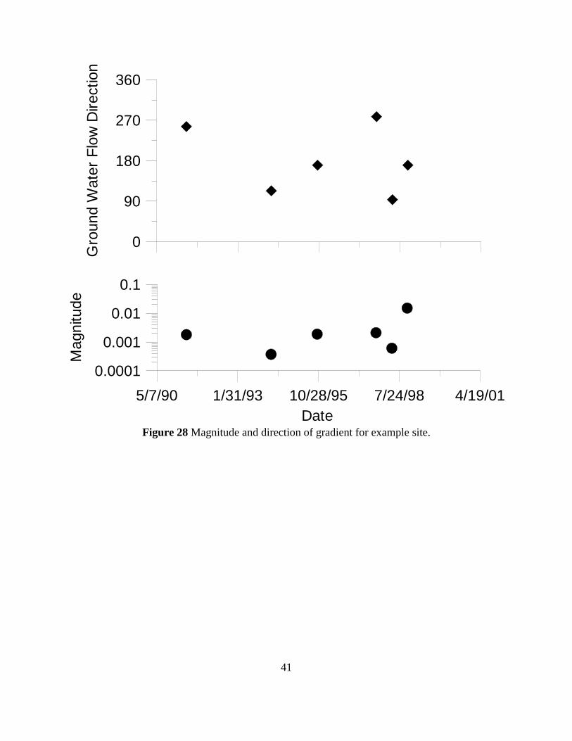
41

0

90

180

270

360G

roun

d W

ater

Flo

w D

irect

ion

5/7/90 1/31/93 10/28/95 7/24/98 4/19/01Date

0.0001

0.001

0.01

0.1

Mag

nitu

de

Figure 28 Magnitude and direction of gradient for example site.

42

Date Well Coordinates (ft) ElevationTOC1

(ft)

Depth toWater (ft)

ElevationWater

(ft)East North

5/7/1991 MW-1 133 99 499.11 48.08 451.03MW-2 123 38 499.19 48.21 450.98MW-3 100 101 498.83 47.87 450.96MW-4 62 89 498.63 47.73 450.9

3/20/1994 MW-1 133 99 499.11 49.27 449.84MW-2 123 38 499.19 49.37 449.82MW-3 100 101 498.83 49.01 449.82MW-4 62 89 498.63 48.77 449.86

10/11/1995 MW-1 133 99 499.11 49.31 449.8MW-2 123 38 499.19 49.52 449.67MW-3 100 101 498.83 49.06 449.77MW-4 62 89 498.63 48.83 449.8

10/8/1997 MW-1 133 99 499.11 48.79 450.32MW-2 123 38 499.19 48.7 450.49MW-3 100 101 498.83 48.2 450.63MW-4 62 89 498.63 48.42 450.21

4/22/1998 MW-1 133 99 499.11 47.99 451.12MW-2 123 38 499.19 48.08 451.11MW-3 100 101 498.83 47.72 451.11MW-4 62 89 498.63 47.47 451.16

10/29/1998 MW-1 133 99 499.11 48.87 450.24MW-2 123 38 499.19 49.89 449.3MW-3 100 101 498.83 48.6 450.23MW-4 62 89 498.63 48.37 450.26

1 TOC stands for top of casing.

Table 11 Data for gradient calculation example.

14http://www.epa.gov/athens/learn2model/part-two/onsite/longdisp.htm

15The converse is also true: it is not possible to prove values are inappropriate in theabsence of fitting.

43

Longitudinal Dispersion Coefficient Calculator14

As discussed previously, the dispersion coefficient appearing in the transport equation(24) represents differential advection, is not measured at LUST sites, and is best treated as afitting parameter. Data have been collected on dispersion coefficients, however, that provideinsight into the dispersion parameter. Gelhar et al. (1992) published a review of dispersivities(D/vs) which is replotted in Figure 29. Because the data do not plot on a horizontal line, Thesedata show scale-dependence of dispersivity. This fact implies that no single value represents acontaminant plume. From this follows the conclusion that dispersivity should be treated as afitting parameter. Various methods have been devised to estimate dispersivity for a specific sitefrom the Gelhar et al. (1992) tabulation. Two of these are shown in Figure 30 (see Xu andEckstein, 1995). Without comparing values generated from these formulas to the underlyingdata, a false sense of certainty may be perceived. At a given scale the tabulated dispersivities canrange over three orders of magnitude. The formulas, of course, give specific values.

In order to give a sense of the formula values and the range of variability, the dispersivitycalculator produces estimates from two formulas, and an evident range from the tabulation. Table 12 gives values for various plume lengths (an indicator of the problem scale) and theestimated range of values in the tabulation. From these results one can conclude that the range ofliterature variability of this parameter is very high and that in the absence of fitting to observedconcentrations there is no way to prove that a chosen value is appropriate.15

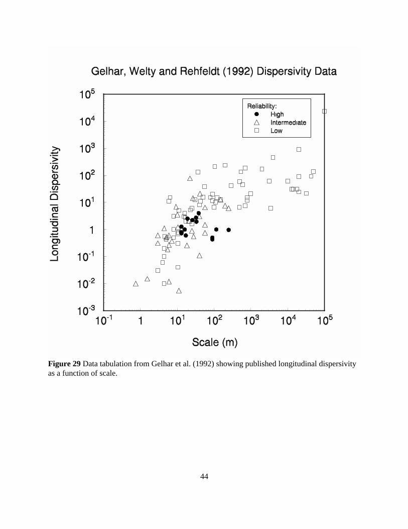
44

Figure 29 Data tabulation from Gelhar et al. (1992) showing published longitudinal dispersivityas a function of scale.

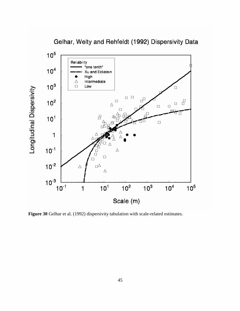
45

Figure 30 Gelhar et al. (1992) dispersivity tabulation with scale-related estimates.

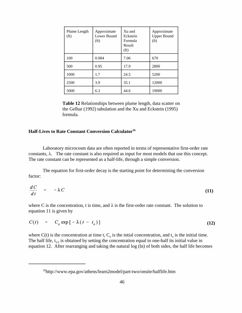
16http://www.epa.gov/athens/learn2model/part-two/onsite/halflife.htm

46

Plume Length(ft)

ApproximateLower Bound(ft)

Xu andEcksteinFormulaResult(ft)

ApproximateUpper Bound(ft)

100 0.084 7.06 670

500 0.95 17.9 2800

1000 1.7 24.5 5200

2500 3.9 35.1 12000

5000 6.3 44.6 19000

Table 12 Relationships between plume length, data scatter onthe Gelhar (1992) tabulation and the Xu and Eckstein (1995)formula.

Half-Lives to Rate Constant Conversion Calculator16

Laboratory microcosm data are often reported in terms of representative first-order rateconstants, 8. The rate constant is also required as input for most models that use this concept. The rate constant can be represented as a half-life, through a simple conversion.

The equation for first-order decay is the starting point for determining the conversionfactor:

(11)

where C is the concentration, t is time, and 8 is the first-order rate constant. The solution toequation 11 is given by

(12)

where C(t) is the concentration at time t, Co is the intial concentration, and to is the initial time. The half life, t1/2 is obtained by setting the concentration equal to one-half its initial value inequation 12. After rearranging and taking the natural log (ln) of both sides, the half life becomes

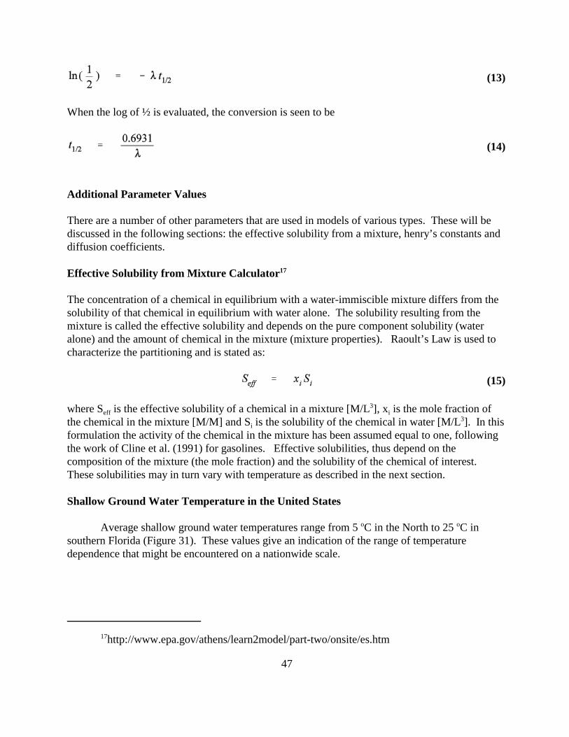
17http://www.epa.gov/athens/learn2model/part-two/onsite/es.htm

47

(13)

When the log of ½ is evaluated, the conversion is seen to be

(14)

Additional Parameter Values

There are a number of other parameters that are used in models of various types. These will bediscussed in the following sections: the effective solubility from a mixture, henry’s constants anddiffusion coefficients.

Effective Solubility from Mixture Calculator17

The concentration of a chemical in equilibrium with a water-immiscible mixture differs from thesolubility of that chemical in equilibrium with water alone. The solubility resulting from themixture is called the effective solubility and depends on the pure component solubility (wateralone) and the amount of chemical in the mixture (mixture properties). Raoult’s Law is used tocharacterize the partitioning and is stated as:

(15)

where Seff is the effective solubility of a chemical in a mixture [M/L3], xi is the mole fraction ofthe chemical in the mixture [M/M] and Si is the solubility of the chemical in water [M/L3]. In thisformulation the activity of the chemical in the mixture has been assumed equal to one, followingthe work of Cline et al. (1991) for gasolines. Effective solubilities, thus depend on thecomposition of the mixture (the mole fraction) and the solubility of the chemical of interest. These solubilities may in turn vary with temperature as described in the next section.

Shallow Ground Water Temperature in the United States

Average shallow ground water temperatures range from 5 oC in the North to 25 oC insouthern Florida (Figure 31). These values give an indication of the range of temperaturedependence that might be encountered on a nationwide scale.

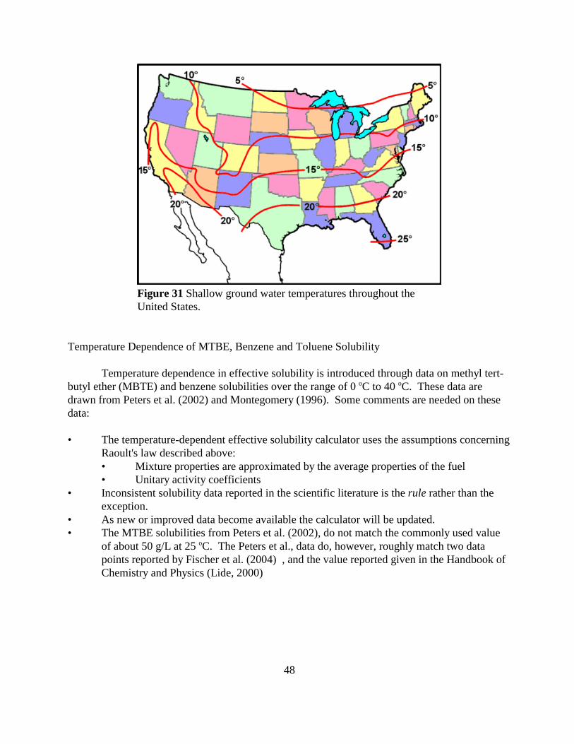
48

Figure 31 Shallow ground water temperatures throughout theUnited States.

Temperature Dependence of MTBE, Benzene and Toluene Solubility

Temperature dependence in effective solubility is introduced through data on methyl tert-butyl ether (MBTE) and benzene solubilities over the range of 0 oC to 40 oC. These data aredrawn from Peters et al. (2002) and Montegomery (1996). Some comments are needed on thesedata:

• The temperature-dependent effective solubility calculator uses the assumptions concerningRaoult's law described above:• Mixture properties are approximated by the average properties of the fuel• Unitary activity coefficients

• Inconsistent solubility data reported in the scientific literature is the rule rather than theexception.

• As new or improved data become available the calculator will be updated.• The MTBE solubilities from Peters et al. (2002), do not match the commonly used value

of about 50 g/L at 25 oC. The Peters et al., data do, however, roughly match two datapoints reported by Fischer et al. (2004) , and the value reported given in the Handbook ofChemistry and Physics (Lide, 2000)

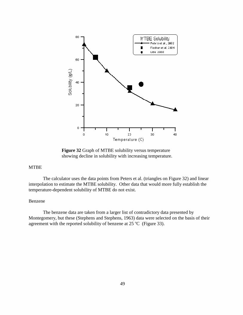
49

Figure 32 Graph of MTBE solubility versus temperatureshowing decline in solubility with increasing temperature.

MTBE

The calculator uses the data points from Peters et al. (triangles on Figure 32) and linearinterpolation to estimate the MTBE solubility. Other data that would more fully establish thetemperature-dependent solubility of MTBE do not exist.

Benzene

The benzene data are taken from a larger list of contradictory data presented byMontegomery, but these (Stephens and Stephens, 1963) data were selected on the basis of theiragreement with the reported solubility of benzene at 25 oC (Figure 33).

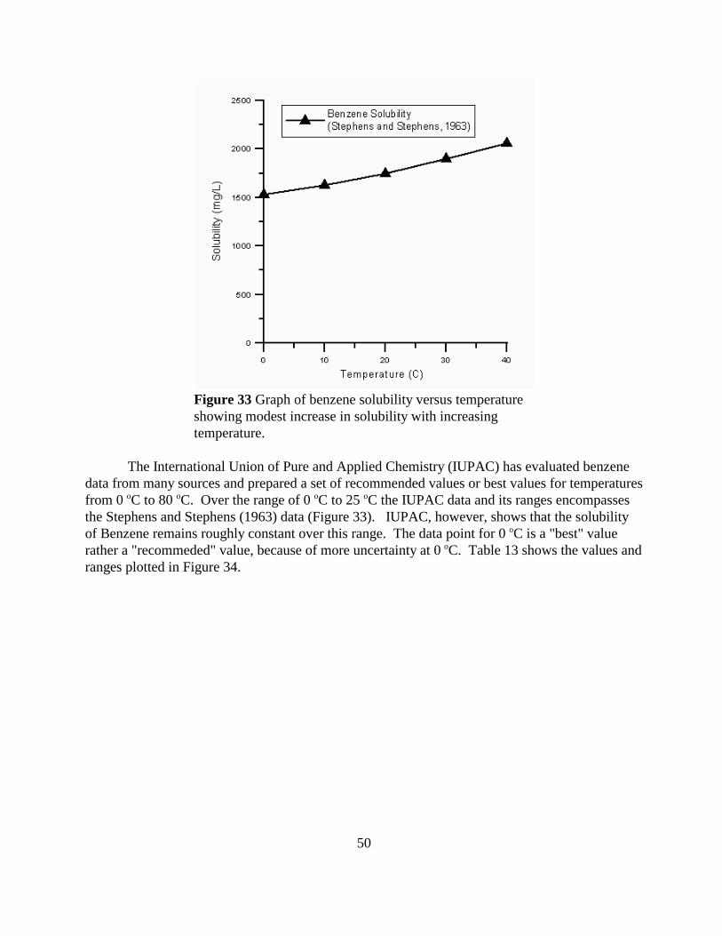
50

Figure 33 Graph of benzene solubility versus temperatureshowing modest increase in solubility with increasingtemperature.

The International Union of Pure and Applied Chemistry (IUPAC) has evaluated benzenedata from many sources and prepared a set of recommended values or best values for temperaturesfrom 0 oC to 80 oC. Over the range of 0 oC to 25 oC the IUPAC data and its ranges encompassesthe Stephens and Stephens (1963) data (Figure 33). IUPAC, however, shows that the solubility of Benzene remains roughly constant over this range. The data point for 0 oC is a "best" valuerather a "recommeded" value, because of more uncertainty at 0 oC. Table 13 shows the values andranges plotted in Figure 34.

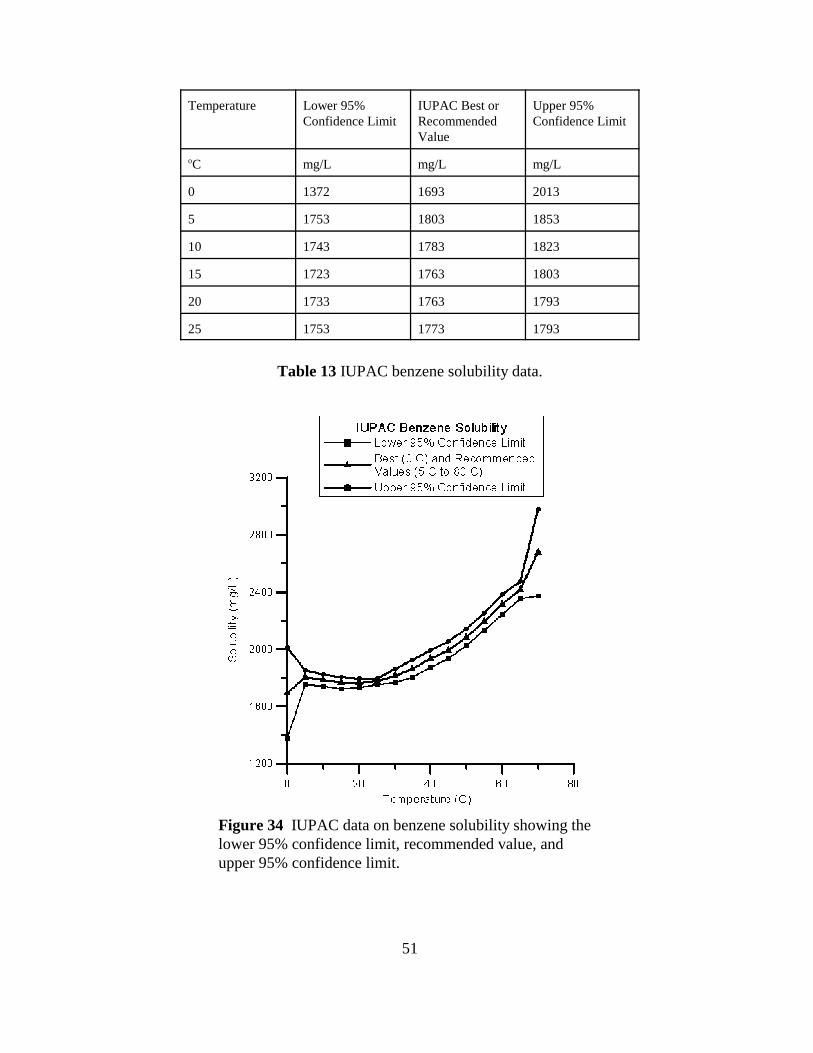
51

Temperature Lower 95%Confidence Limit

IUPAC Best orRecommendedValue

Upper 95%Confidence Limit

oC mg/L mg/L mg/L

0 1372 1693 2013

5 1753 1803 1853

10 1743 1783 1823

15 1723 1763 1803

20 1733 1763 1793

25 1753 1773 1793

Table 13 IUPAC benzene solubility data.

Figure 34 IUPAC data on benzene solubility showing thelower 95% confidence limit, recommended value, andupper 95% confidence limit.

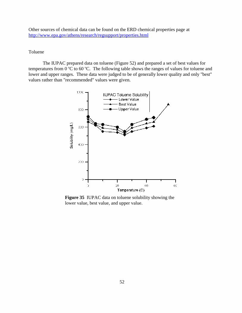
52

Other sources of chemical data can be found on the ERD chemical properties page athttp://www.epa.gov/athens/research/regsupport/properties.html

Toluene

The IUPAC prepared data on toluene (Figure 52) and prepared a set of best values fortemperatures from 0 oC to 60 oC. The following table shows the ranges of values for toluene andlower and upper ranges. These data were judged to be of generally lower quality and only "best"values rather than "recommended" values were given.

Figure 35 IUPAC data on toluene solubility showing thelower value, best value, and upper value.

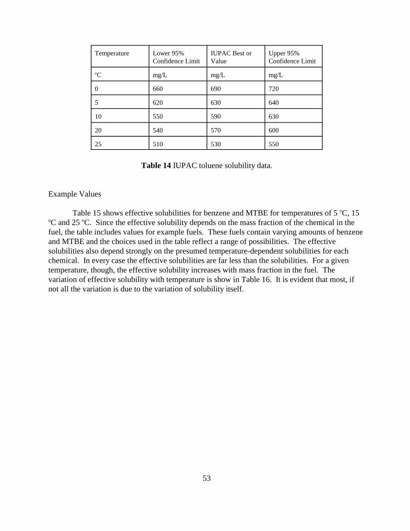
53

Temperature Lower 95%Confidence Limit

IUPAC Best orValue

Upper 95%Confidence Limit

oC mg/L mg/L mg/L

0 660 690 720

5 620 630 640

10 550 590 630

20 540 570 600

25 510 530 550

Table 14 IUPAC toluene solubility data.

Example Values

Table 15 shows effective solubilities for benzene and MTBE for temperatures of 5 oC, 15oC and 25 oC. Since the effective solubility depends on the mass fraction of the chemical in thefuel, the table includes values for example fuels. These fuels contain varying amounts of benzeneand MTBE and the choices used in the table reflect a range of possibilities. The effectivesolubilities also depend strongly on the presumed temperature-dependent solubilities for eachchemical. In every case the effective solubilities are far less than the solubilities. For a giventemperature, though, the effective solubility increases with mass fraction in the fuel. Thevariation of effective solubility with temperature is show in Table 16. It is evident that most, ifnot all the variation is due to the variation of solubility itself.

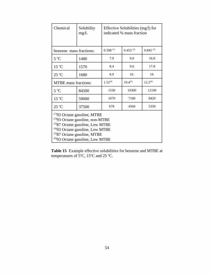
54

Chemical Solubilitymg/L

Effective Solubilities (mg/l) forindicated % mass fraction

benzene mass fractions: 0.398 (1) 0.453 (2) 0.845 (3)

5 oC 1480 7.9 9.0 16.8

15 oC 1570 8.4 9.6 17.8

25 oC 1680 8.9 10. 19.

MTBE mass fractions: 1.52(4) 10.4(5) 12.2(6)

5 oC 84500 1530 10300 12100

15 oC 59000 1070 7180 8420

25 oC 37500 678 4560 5350

(1)93 Octane gasoline, MTBE(2)93 Octane gasoline, non-MTBE(3)87 Octane gasoline, Low MTBE(4)93 Octane gasoline, Low MTBE(5)87 Octane gasoline, MTBE(6)93 Octane gasoline, Low MTBE

Table 15 Example effective solubilities for benzene and MTBE attemperatures of 5oC, 15oC and 25 oC.

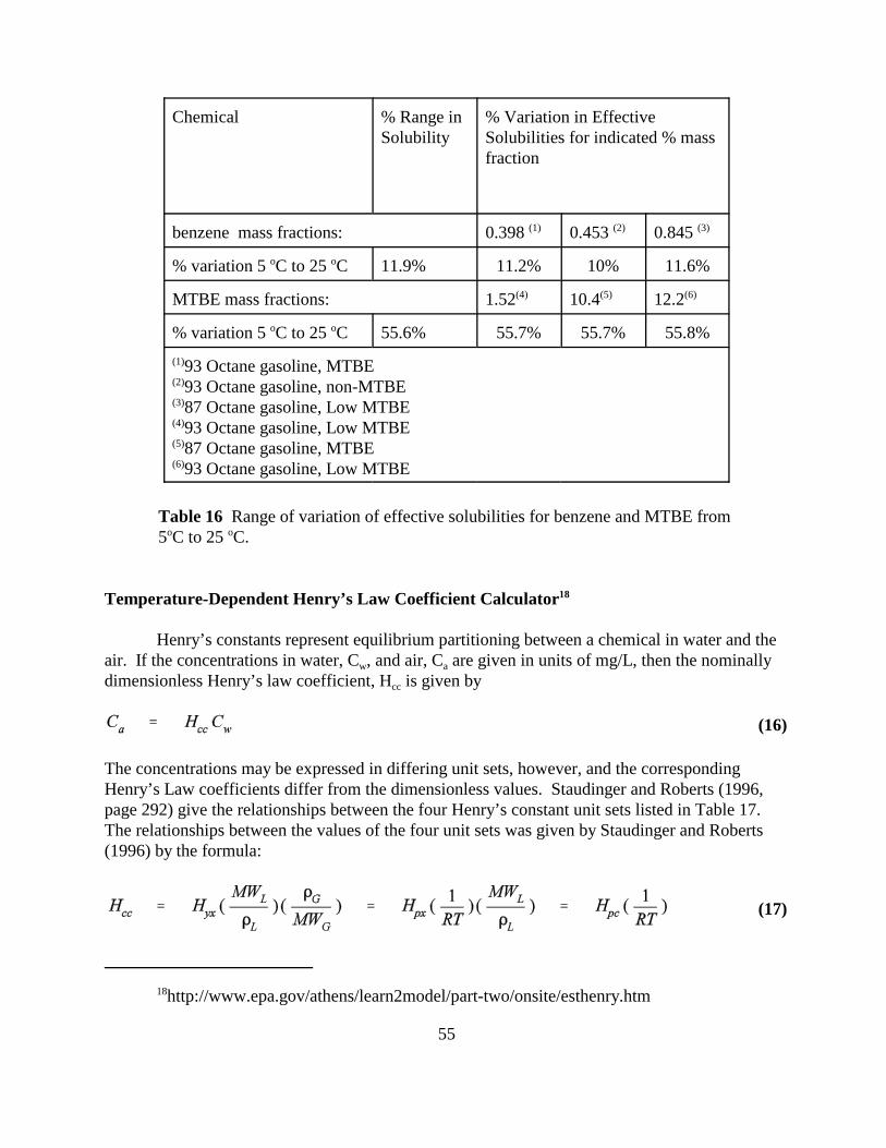
18http://www.epa.gov/athens/learn2model/part-two/onsite/esthenry.htm

55

Chemical % Range in Solubility

% Variation in EffectiveSolubilities for indicated % massfraction

benzene mass fractions: 0.398 (1) 0.453 (2) 0.845 (3)

% variation 5 oC to 25 oC 11.9% 11.2% 10% 11.6%

MTBE mass fractions: 1.52(4) 10.4(5) 12.2(6)

% variation 5 oC to 25 oC 55.6% 55.7% 55.7% 55.8%(1)93 Octane gasoline, MTBE(2)93 Octane gasoline, non-MTBE(3)87 Octane gasoline, Low MTBE(4)93 Octane gasoline, Low MTBE(5)87 Octane gasoline, MTBE(6)93 Octane gasoline, Low MTBE

Table 16 Range of variation of effective solubilities for benzene and MTBE from 5oC to 25 oC.

Temperature-Dependent Henry’s Law Coefficient Calculator18

Henry’s constants represent equilibrium partitioning between a chemical in water and theair. If the concentrations in water, Cw, and air, Ca are given in units of mg/L, then the nominallydimensionless Henry’s law coefficient, Hcc is given by

(16)

The concentrations may be expressed in differing unit sets, however, and the correspondingHenry’s Law coefficients differ from the dimensionless values. Staudinger and Roberts (1996,page 292) give the relationships between the four Henry’s constant unit sets listed in Table 17. The relationships between the values of the four unit sets was given by Staudinger and Roberts(1996) by the formula:

(17)

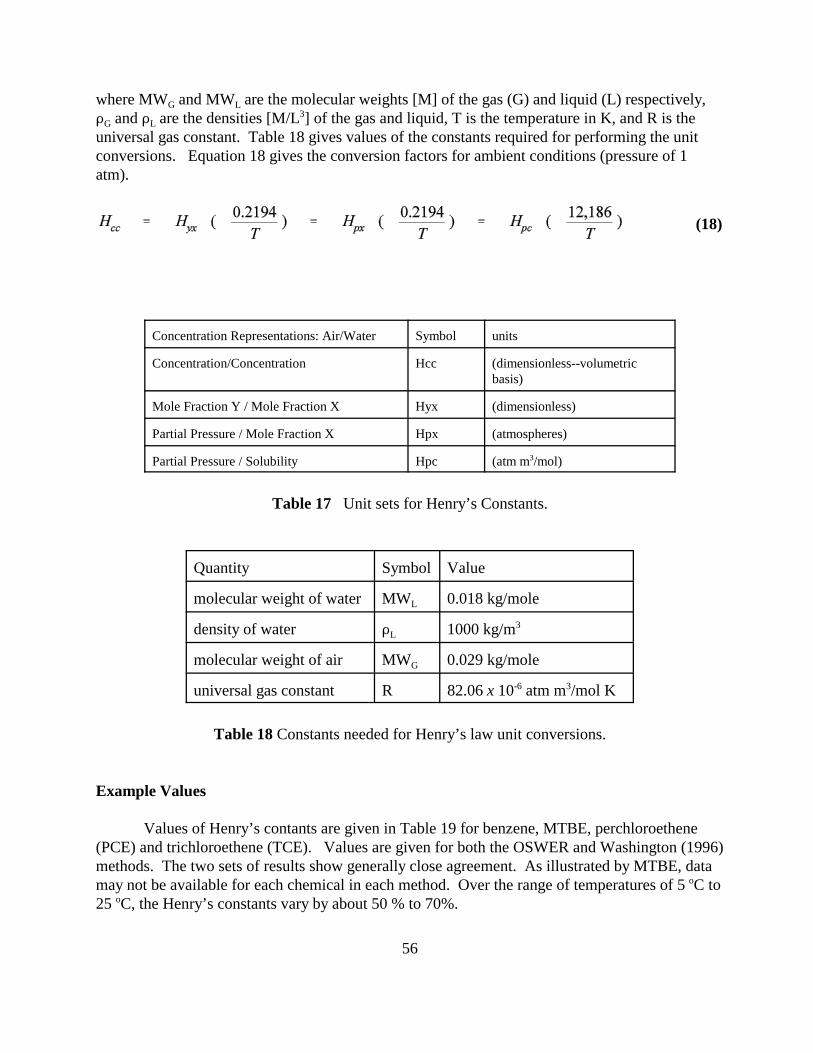
56

where MWG and MWL are the molecular weights [M] of the gas (G) and liquid (L) respectively,DG and DL are the densities [M/L3] of the gas and liquid, T is the temperature in K, and R is theuniversal gas constant. Table 18 gives values of the constants required for performing the unitconversions. Equation 18 gives the conversion factors for ambient conditions (pressure of 1atm).

(18)

Concentration Representations: Air/Water Symbol units

Concentration/Concentration Hcc (dimensionless--volumetricbasis)

Mole Fraction Y / Mole Fraction X Hyx (dimensionless)

Partial Pressure / Mole Fraction X Hpx (atmospheres)

Partial Pressure / Solubility Hpc (atm m3/mol)

Table 17 Unit sets for Henry’s Constants.

Quantity Symbol Value

molecular weight of water MWL 0.018 kg/mole

density of water DL 1000 kg/m3

molecular weight of air MWG 0.029 kg/mole

universal gas constant R 82.06 x 10-6 atm m3/mol K

Table 18 Constants needed for Henry’s law unit conversions.

Example Values

Values of Henry’s contants are given in Table 19 for benzene, MTBE, perchloroethene(PCE) and trichloroethene (TCE). Values are given for both the OSWER and Washington (1996)methods. The two sets of results show generally close agreement. As illustrated by MTBE, datamay not be available for each chemical in each method. Over the range of temperatures of 5 oC to25 oC, the Henry’s constants vary by about 50 % to 70%.

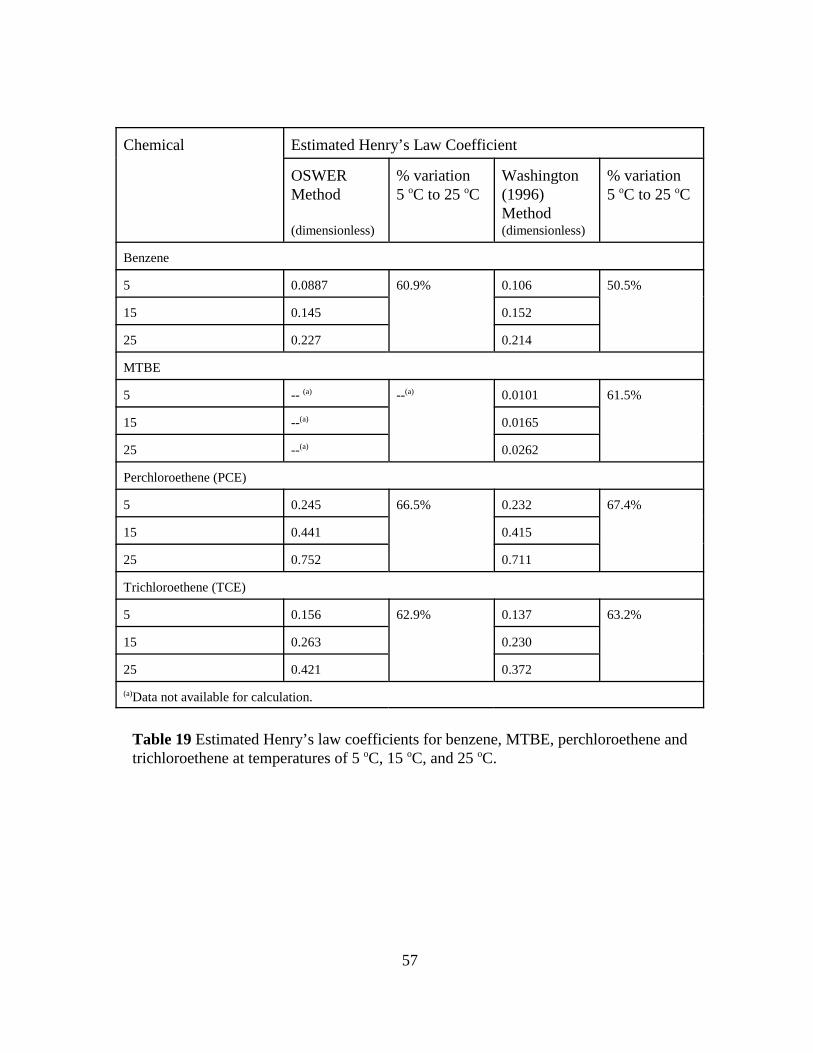
57

Chemical Estimated Henry’s Law Coefficient

OSWERMethod

(dimensionless)

% variation5 oC to 25 oC

Washington(1996)Method(dimensionless)

% variation5 oC to 25 oC

Benzene

5 0.0887 60.9% 0.106 50.5%

15 0.145 0.152

25 0.227 0.214

MTBE

5 -- (a) --(a) 0.0101 61.5%

15 --(a) 0.0165

25 --(a) 0.0262

Perchloroethene (PCE)

5 0.245 66.5% 0.232 67.4%

15 0.441 0.415

25 0.752 0.711

Trichloroethene (TCE)

5 0.156 62.9% 0.137 63.2%

15 0.263 0.230

25 0.421 0.372

(a)Data not available for calculation.

Table 19 Estimated Henry’s law coefficients for benzene, MTBE, perchloroethene andtrichloroethene at temperatures of 5 oC, 15 oC, and 25 oC.

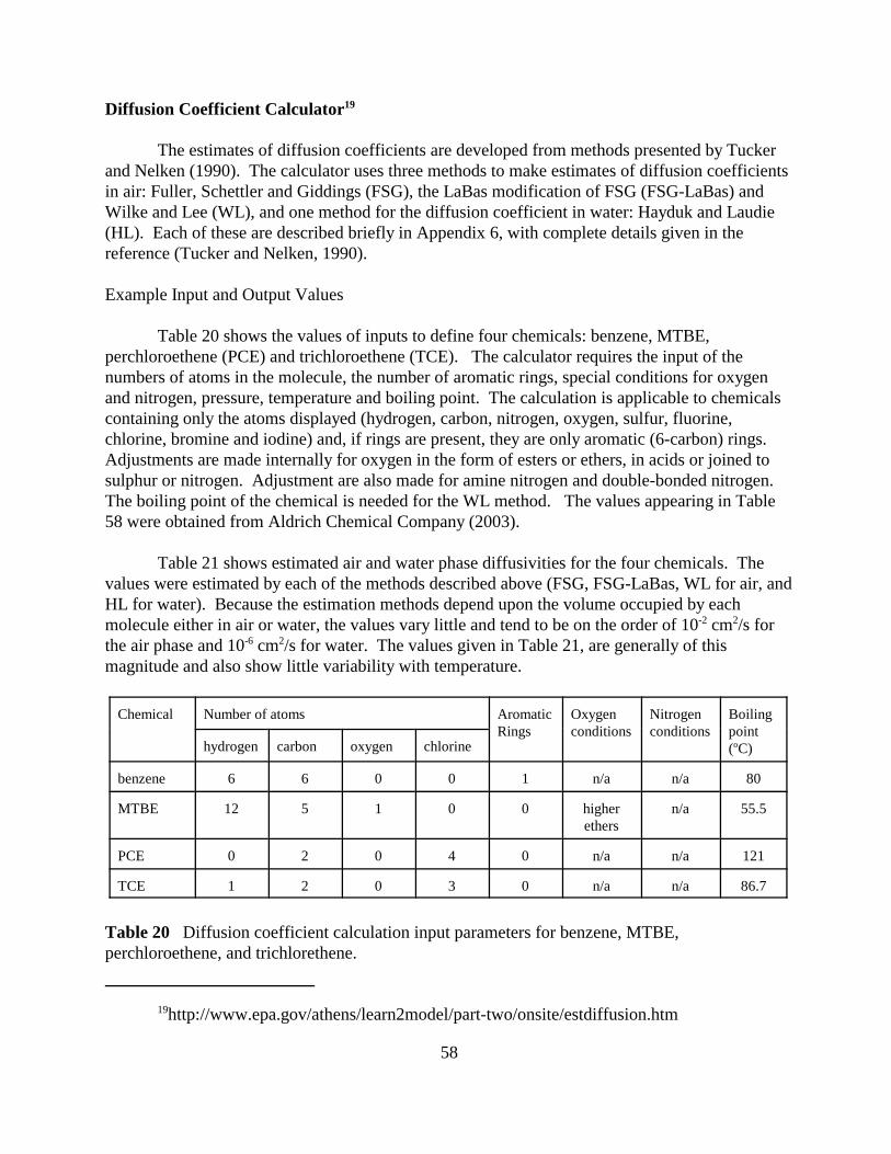
19http://www.epa.gov/athens/learn2model/part-two/onsite/estdiffusion.htm

58

Diffusion Coefficient Calculator19

The estimates of diffusion coefficients are developed from methods presented by Tuckerand Nelken (1990). The calculator uses three methods to make estimates of diffusion coefficientsin air: Fuller, Schettler and Giddings (FSG), the LaBas modification of FSG (FSG-LaBas) andWilke and Lee (WL), and one method for the diffusion coefficient in water: Hayduk and Laudie(HL). Each of these are described briefly in Appendix 6, with complete details given in thereference (Tucker and Nelken, 1990).

Example Input and Output Values

Table 20 shows the values of inputs to define four chemicals: benzene, MTBE,perchloroethene (PCE) and trichloroethene (TCE). The calculator requires the input of thenumbers of atoms in the molecule, the number of aromatic rings, special conditions for oxygenand nitrogen, pressure, temperature and boiling point. The calculation is applicable to chemicalscontaining only the atoms displayed (hydrogen, carbon, nitrogen, oxygen, sulfur, fluorine,chlorine, bromine and iodine) and, if rings are present, they are only aromatic (6-carbon) rings. Adjustments are made internally for oxygen in the form of esters or ethers, in acids or joined tosulphur or nitrogen. Adjustment are also made for amine nitrogen and double-bonded nitrogen. The boiling point of the chemical is needed for the WL method. The values appearing in Table58 were obtained from Aldrich Chemical Company (2003).

Table 21 shows estimated air and water phase diffusivities for the four chemicals. Thevalues were estimated by each of the methods described above (FSG, FSG-LaBas, WL for air, andHL for water). Because the estimation methods depend upon the volume occupied by eachmolecule either in air or water, the values vary little and tend to be on the order of 10-2 cm2/s forthe air phase and 10-6 cm2/s for water. The values given in Table 21, are generally of thismagnitude and also show little variability with temperature.

Chemical Number of atoms AromaticRings

Oxygen conditions

Nitrogen conditions

Boilingpoint(oC)hydrogen carbon oxygen chlorine

benzene 6 6 0 0 1 n/a n/a 80

MTBE 12 5 1 0 0 higherethers

n/a 55.5

PCE 0 2 0 4 0 n/a n/a 121

TCE 1 2 0 3 0 n/a n/a 86.7

Table 20 Diffusion coefficient calculation input parameters for benzene, MTBE,perchloroethene, and trichlorethene.

59

Chemical Diffusion Coefficients in Air(cm2/s)

DiffusionCoefficient inWater(cm2/s)

FSG FSG-LaBas

WL HL

Benzene

5 oC 0.0792 0.0817 0.0859 5.6 e-6

15 oC 0.0842 0.0869 0.0919 7.8 e-6

25 oC 0.0894 0.0923 0.0980 1.0 e-5

MTBE

5 oC 0.0714 0.0710 0.0751 4.7 e-6

15 oC 0.0759 0.0755 0.0803 6.5 e-6

25 oC 0.0806 0.0802 0.0856 8.6 e-6

Perchloroethene (PCE)

5 oC 0.0673 0.0671 0.0711 4.7 e-6

15 oC 0.0716 0.0713 0.0760 6.6 e-6

25 oC 0.0760 0.0757 0.0811 8.7 e-7

Trichloroethene (TCE)

5 oC 0.0738 0.0737 0.0779 5.3 e-6

15 oC 0.0785 0.0784 0.0832 7.3 e-6

25 oC 0.0833 0.0832 0.0888 9.7 e-6

Table 21 Estimated air and water diffusivities for benzene, MTBE,perchloroethene and trichloroethene at temperatures of 5 oC, 15 oC, and 25 oC.

60

5. Conclusions

A series of on-line tools has been created for assisting in assessing contaminated sites.These tools include simple methods for estimating model inputs. The direct model input toolsinclude the retardation factor, hydraulic gradient, seepage velocity, dispersion coefficients, rateconstant/half life conversions. Other tools provide methods and data for estimating the effectivesolubility of contaminants from fuels, temperature-dependent Henry’s constants, and air and waterphase diffusivities. These parameters are needed for certain models and the effective solubilitycan be sued to determine the maximum possible concentration resulting from fuel contamination.

Because few sites are evaluated based on field data alone, models or other calculations areused in site assessment. As stated previously, models are chosen for this task because

• they have an evident ability to predict future concentrations,• they have a scientific basis, • they have the ability to include the effects of many different factors, and• they have become accepted as predictive tools.

A number of factors, however, influence and limit the ability of models to predict futurecontamination. This report focused on uncertainty in parameter values. For the prediction ofplume diving, recharge estimates are critical, but may be difficult to obtain. Here the model isused as a tool for the best placement of well screens. Subsequent data collection would confirmthe prediction, but, more importantly, would be of higher quality because of the inclusion of thistheory in well placement. Parameter uncertainty in contaminant transport showed that a widevariety of breakthrough curves could be generated from a set of inputs. Where the inputs are notcompletely know, this behavior of the model is a truer representation of the results than a modelrun using averaged parameters. If, however, through uncertainty analysis it can be shown thatgeneric best and worst cases exist, then bounding results could be generated. For the one-dimensional contaminant transport model studied here, generic worst/best cases can be establishedfor the first arrival time, maximum concentration and duration. The parameter sets that generatethese do not generate each of the worst/best cases. When risk is considered to be based ontransient concentrations, a generic worst case doesn’t exist at all. For these two reasons theexistence of universal extreme parameter sets it limited, but may be useful in some cases.

61

References

Aldrich Chemical Company, 2003 Aldrich Handbook of Fine Chemicals and LaboratoryEquipment.

ASTM, 1995, Standard Guide for Risk-Based Corrective Action Applied at Petroleum ReleaseSites, American Society for Testing and Materials, ASTM Designation E 1739095.

Bear, J., 1972, Dynamics o f Fluids in Porous Media, American Elsevier, New York.

Buscheck, T.E. and C.M. Alacantar, 1995, Regression Techniques and Analytical Solutions toDemonstrate Intrinsic Bioremediation, Intrinsic Bioremediation, Hinchee, R.E., J.T. Wilson, D.C.Downey, eds., Battelle Press, 3(1).

Cline, P.V., J.J. Delfino, P.S.C. Rao, 1991, Partitioning of aromatic constituents into water fromgasoline and other complex solvent mixtures, Environmental Science and Technology, 23, 914-920.

Eggleston, J.R. and S. A. Rojstaczer, 2000, Can We Predict Subsurface Mass Transport?,Environmental Science and Technology, 34, 4010-4017.

Fischer, A., M. Muller, J. Klasmeier, 2004, Determination of Henry's law constant for methyl tert-butyl ether (MTBE) at groundwater temperatures, Chemosphere, 54, 689-694.

Gelhar, L.W., K.R. Rehfeldt, and C.A. Welty, 1992, A critical review of data on field-scaledispersion in aquifers, Water Resources Research, 28(7), 1955-1974.

Haitjema, H.M., 1995, Analytic Element Modeling of Groundwater Flow, Academic Press,304pp.

Leij, F.J. and S.A. Bradford, 1994, 3DADE:A computer program for evaluating three-dimensionalequilibrium solute transport in porous media, Research Report No. 134, U.S. Salinity Laboratory,Riverside, CA.

Lide, D.R., 2000, CRC Handbook of Chemistry and Physics, 81st ed., CRC Press, page 8-95.

Miller, C.T. and W.G. Gray, 2002, Hydrological Research: Just Getting Started, Ground Water,40(3), 224-231.

Montegomery, J.H., 1996, Groundwater Chemicals Desk Reference, 2nd ed., CRC Press, LewisPublishers, Boca Raton, Florida, page 70-71.

Oreskes, N., K. Shrader-Frechette, K. Belitz, 1994, Verification, Validation, and Confirmation ofNumerical Models in the Earth Sciences, Science, 263, 641-646.

62

Peters, U., F. Nierlich, M. Sakuth, and M. Laugier, 2002, Methyl Tert-Butyl Ether, Physical andChemical Properties, Ullmanns Encyclopedia of Industrial Chemistry, Release 2003, 6th ed., VCH Verlag GmbH & Co. KGaA, Wiley, DOI, 10.1002/14356007.a16_543.

Shaw, D.G., 1989, Solubility Data Series, Hydrocarbon with Water and Seawater, Part I: Hydrocarbons C5 to C7, Volume 37, International Union of Pure and Applied Chemistry,Pergamon Press, Oxford.

Strack, O.D.L., 1984, Three-dimensional streamlines in Dupuit-Forchheimer models, WaterResources Research, 20, 812-822.

Staudinger and Roberts, 1996, A Critical Review of Henry's Law Constants for EnvironmentalApplications, in Critical Reviews in Environmental Science and Technology, 26(3):205-297

Stephen, H. and T. Stephen, 1963, Solubilities of Inorganic and Organic Compounds, Vol. 1.,Macmillan, New York.

Tucker, W.A., and L.H. Nelken, 1990, Chapter 17: Diffusion Coefficients in Air and Water,Handbook of Chemical Property Estimation Methods. Warren J. Lyman, William F. Reehl andDavid H. Rosenblatt, eds., first edition, American Chemical Society.

United States Environmental Protection Agency, 1989, Risk Assessment Guidance for SuperfundVolume 1, Human Health Evaluation Manual (Part A), Interim Final, Office of Emergency andRemedial Response, Washington, DC, EPA/540/1-89-002.

United States Environmental Protection Agency, 2001, Fact Sheet: Correcting the Henry’s LawCoefficient for Temperature, Office of Solid Waste and Emergency Response,http://www.epa.gov/athens/learn2model/part-two/onsite/doc/factsheet.pdf.

van Genuchten, M. T. and W. J. Alves, 1982, Analytical Solutions of the One-DimensionalConvective-Dispersive Solute Transport Equation, United States Department of Agriculture,Agricultural Research Service, Technical Bulletin Number 1661.

Washington, J., 1996, Gas partitioning of dissolved volatile organic compounds in the vadosezone: Principles, temperature effects and literature review, Ground Water, 34(4), 709-718.

Weaver, J.W, J.T. Haas, and J.T. Wilson, 1996, Analysis of the gasoline spill at East Patchogue,New York, Procedings of Non-Aqueous Phase Liquids (NAPLs) in Subsurface Environment:Assessment and Remediation, ed. L. Reddi, American Society of Civil Engineers, Washington,D.C., November 12-14, pp. 707-718.

Weaver, J.W, 1996, Application of the Hydrocarbon Spill Screening Model to Field Sites,Procedings of Non-Aqueous Phase Liquids (NAPLs) in Subsurface Environment: Assessment and

63

Remediation, ed. L. Reddi, American Society of Civil Engineers, Washington, D.C., November12-14, pp. 788-799.

Xu, M., and Y. Eckstein, 1995, Use of weighted least-squares method in evaluation of therelationship between dispersivity and scale, Groundwater, 33(6), 905-908.

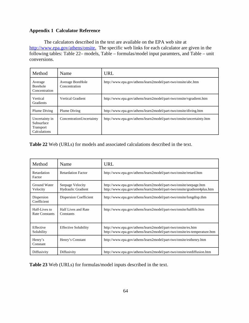
64

Appendix 1 Calculator Reference

The calculators described in the text are available on the EPA web site athttp://www.epa.gov/athens/onsite. The specific web links for each calculator are given in thefollowing tables: Table 22– models, Table – formulas/model input paramters, and Table – unitconversions.

Method Name URL

AverageBoreholeConcentration

Average BoreHoleConcentration

http://www.epa.gov/athens/learn2model/part-two/onsite/abc.htm

VerticalGradients

Vertical Gradient http://www.epa.gov/athens/learn2model/part-two/onsite/vgradient.htm

Plume Diving Plume Diving http://www.epa.gov/athens/learn2model/part-two/onsite/diving.htm

Uncertainty inSubsurfaceTransportCalculations

ConcentrationUncertainty http://www.epa.gov/athens/learn2model/part-two/onsite/uncertainty.htm

Table 22 Web (URLs) for models and associated calculations described in the text.

Method Name URL

RetardationFactor

Retardation Factor http://www.epa.gov/athens/learn2model/part-two/onsite/retard.htm

Ground WaterVelocity

Seepage VelocityHydraulic Gradient

http://www.epa.gov/athens/learn2model/part-two/onsite/seepage.htmhttp://www.epa.gov/athens/learn2model/part-two/onsite/gradient4plus.htm

DispersionCoefficient

Dispersion Coefficient http://www.epa.gov/athens/learn2model/part-two/onsite/longdisp.thm

Half-Lives toRate Constants

Half Lives and RateConstants

http://www.epa.gov/athens/learn2model/part-two/onsite/halflife.htm

EffectiveSolubility

Effective Solubility http://www.epa.gov/athens/learn2model/part-two/onsite/es.htmhttp://www.epa.gov/athens/learn2model/part-two/onsite/es-temperature.htm

Henry’sConstant

Henry’s Constant http://www.epa.gov/athens/learn2model/part-two/onsite/esthenry.htm

Diffusivity Diffusivity http://www.epa.gov/athens/learn2model/part-two/onsite/estdiffusion.htm

Table 23 Web (URLs) for formulas/model inputs described in the text.

65

Appendix 2 Acronyms and Abbreviations

BTEX Benzene, toluene, ethylbenzene and xylenesCoC Concentration-of-concernFSG Fuller, Schettler and Giddings Method for Air DiffusionIUPAC International Union of Pure and Applied ChemistryHL Hayduk and Laudie Method for Water DiffusionLUST Leaking underground storage tankMCL Maximum contaminant levelMTBE Methyl tert-butyl etherPCE PerchloroetheneTCE TrichloroetheneTOC Top of casingURL Uniform Resource LocatorWL Wilke and Lee Method for Air Diffusion

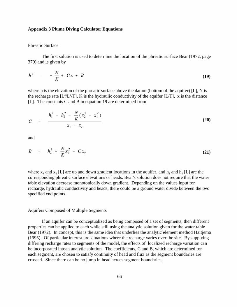
66

Appendix 3 Plume Diving Calculator Equations

Phreatic Surface

The first solution is used to determine the location of the phreatic surface Bear (1972, page379) and is given by

(19)

where h is the elevation of the phreatic surface above the datum (bottom of the aquifer) [L], N isthe recharge rate [L3/L2/T], K is the hydraulic conductivity of the aquifer [L/T], x is the distance[L]. The constants C and B in equation 19 are determined from

(20)

and

(21)

where x1 and x2 [L] are up and down gradient locations in the aquifer, and h1 and h2 [L] are thecorresponding phreatic surface elevations or heads. Bear's solution does not require that the watertable elevation decrease monotonically down gradient. Depending on the values input forrecharge, hydraulic conductivity and heads, there could be a ground water divide between the twospecified end points.

Aquifers Composed of Multiple Segments

If an aquifer can be conceptualized as being composed of a set of segments, then differentproperties can be applied to each while still using the analytic solution given for the water tableBear (1972). In concept, this is the same idea that underlies the analytic element method Haitjema(1995). Of particular interest are situations where the recharge varies over the site. By supplyingdiffering recharge rates to segments of the model, the effects of localized recharge variation canbe incorporated intoan analytic solution. The coefficients, C and B, which are determined foreach segment, are chosen to satisfy continuity of head and flux as the segment boundaries arecrossed. Since there can be no jump in head across segment boundaries,

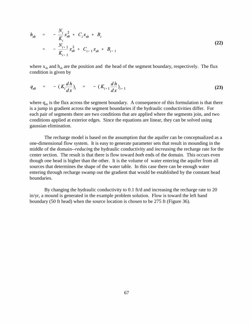
67

(22)

where xsb and hsb are the position and the head of the segment boundary, respectively. The fluxcondition is given by

(23)

where qsb is the flux across the segment boundary. A consequence of this formulation is that thereis a jump in gradient across the segment boundaries if the hydraulic conductivities differ. Foreach pair of segments there are two conditions that are applied where the segments join, and twoconditions applied at exterior edges. Since the equations are linear, they can be solved usinggaussian elimination.

The recharge model is based on the assumption that the aquifer can be conceptualized as aone-dimensional flow system. It is easy to generate parameter sets that result in mounding in themiddle of the domain--reducing the hydraulic conductivity and increasing the recharge rate for thecenter section. The result is that there is flow toward both ends of the domain. This occurs eventhough one head is higher than the other. It is the volume of water entering the aquifer from allsources that determines the shape of the water table. In this case there can be enough waterentering through recharge swamp out the gradient that would be established by the constant headboundaries.

By changing the hydraulic conductivity to 0.1 ft/d and increasing the recharge rate to 20in/yr, a mound is generated in the example problem solution. Flow is toward the left handboundary (50 ft head) when the source location is chosen to be 275 ft (Figure 36).

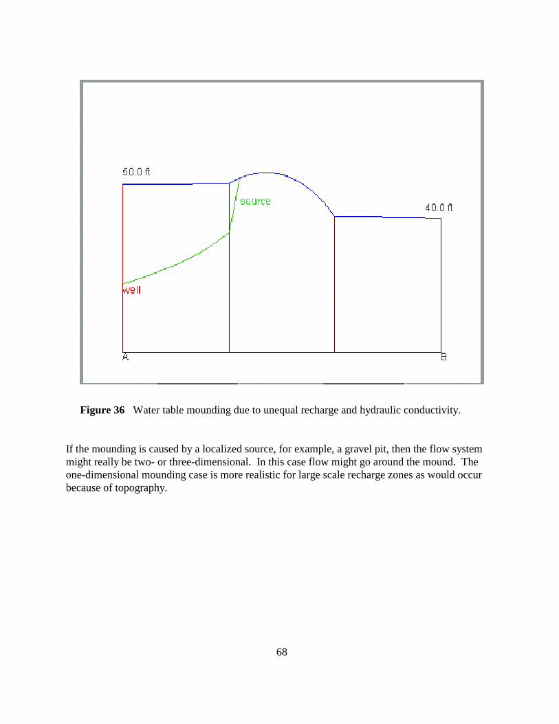
68

Figure 36 Water table mounding due to unequal recharge and hydraulic conductivity.

If the mounding is caused by a localized source, for example, a gravel pit, then the flow systemmight really be two- or three-dimensional. In this case flow might go around the mound. Theone-dimensional mounding case is more realistic for large scale recharge zones as would occurbecause of topography.

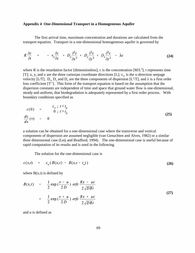
69

Appendix 4 One-Dimensional Transport in a Homogeneous Aquifer

The first arrival time, maximum concentration and durations are calculated from thetransport equation. Transport in a one-dimensional homogeneous aquifer is governed by

(24)

where R is the retardation factor [dimensionless], c is the concentration [M/L3]; t represents time[T]; x, y, and z are the three cartesian coordinate directions [L]; vx, is the x-direction seepagevelocity [L/T], Dx, Dy and Dx are the three components of dispersion [L2/T], and 8 is a first orderloss coefficient [T-1]. This form of the transport equation is based on the assumption that thedispersion constants are independent of time and space that ground water flow is one-dimensional,steady and uniform, that biodegradation is adequately represented by a first order process. Withboundary conditions specified as

(25)

a solution can be obtained for a one-dimensional case where the transverse and verticalcomponents of dispersion are assumed negligible (van Genuchten and Alves, 1982) or a similarthree dimensional case (Leij and Bradford, 1994). The one-dimensional case is useful because ofrapid computation of its results and is used in the following.

The solution for the one-dimensional case is

(26)

where B(x,t) is defined by

(27)

and u is defined as

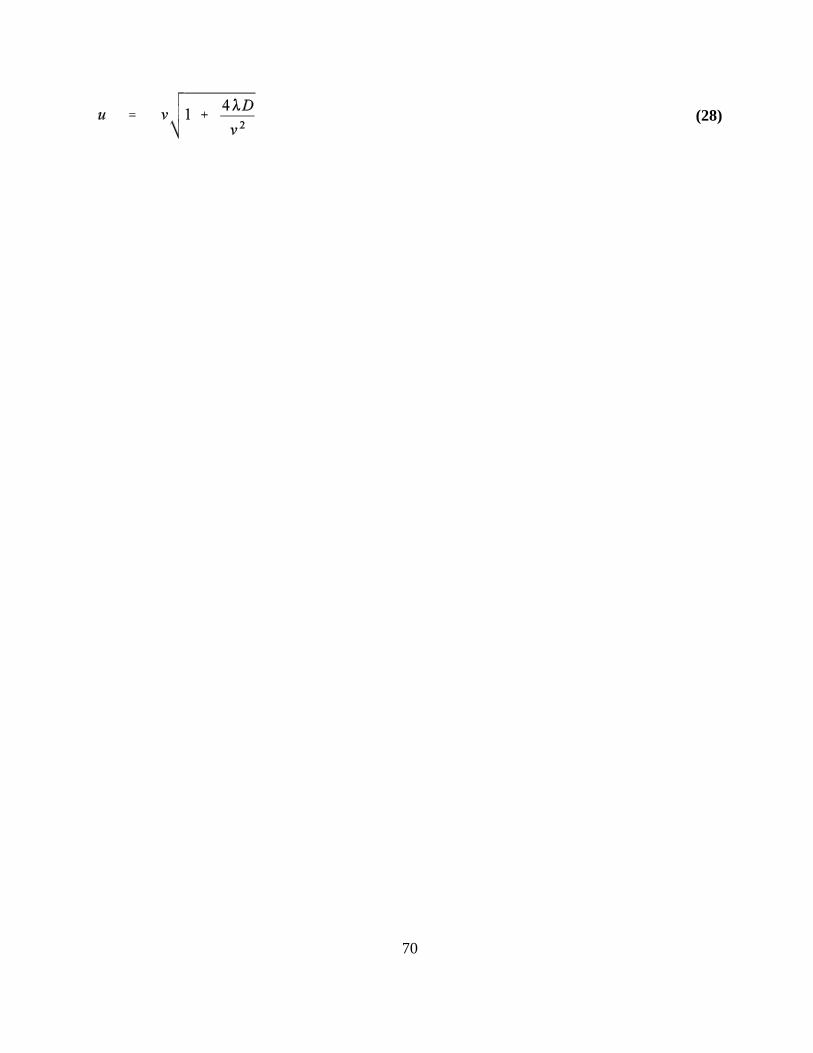
70

(28)

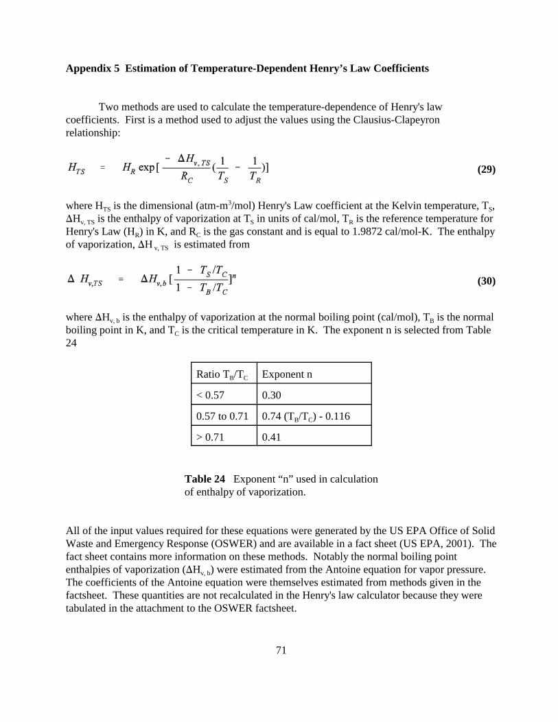
71

Appendix 5 Estimation of Temperature-Dependent Henry’s Law Coefficients

Two methods are used to calculate the temperature-dependence of Henry's lawcoefficients. First is a method used to adjust the values using the Clausius-Clapeyronrelationship:

(29)

where HTS is the dimensional (atm-m3/mol) Henry's Law coefficient at the Kelvin temperature, TS,)Hv, TS is the enthalpy of vaporization at TS in units of cal/mol, TR is the reference temperature forHenry's Law (HR) in K, and RC is the gas constant and is equal to 1.9872 cal/mol-K. The enthalpyof vaporization, )H v, TS is estimated from

(30)

where )Hv, b is the enthalpy of vaporization at the normal boiling point (cal/mol), TB is the normalboiling point in K, and TC is the critical temperature in K. The exponent n is selected from Table24

Ratio TB/TC Exponent n

< 0.57 0.30

0.57 to 0.71 0.74 (TB/TC) - 0.116

> 0.71 0.41

Table 24 Exponent “n” used in calculationof enthalpy of vaporization.

All of the input values required for these equations were generated by the US EPA Office of SolidWaste and Emergency Response (OSWER) and are available in a fact sheet (US EPA, 2001). Thefact sheet contains more information on these methods. Notably the normal boiling pointenthalpies of vaporization ()Hv, b) were estimated from the Antoine equation for vapor pressure. The coefficients of the Antoine equation were themselves estimated from methods given in thefactsheet. These quantities are not recalculated in the Henry's law calculator because they weretabulated in the attachment to the OSWER factsheet.

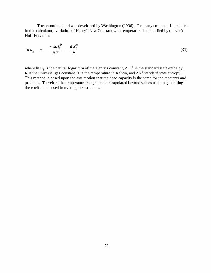
72

The second method was developed by Washington (1996). For many compounds includedin this calculator, variation of Henry's Law Constant with temperature is quantified by the van'tHoff Equation:

(31)

where ln Kh is the natural logarithm of the Henry's constant, )Hr2 is the standard state enthalpy,

R is the universal gas constant, T is the temperature in Kelvin, and )Sr2 standard state entropy.

This method is based upon the assumption that the head capacity is the same for the reactants andproducts. Therefore the temperature range is not extrapolated beyond values used in generatingthe coefficients used in making the estimates.

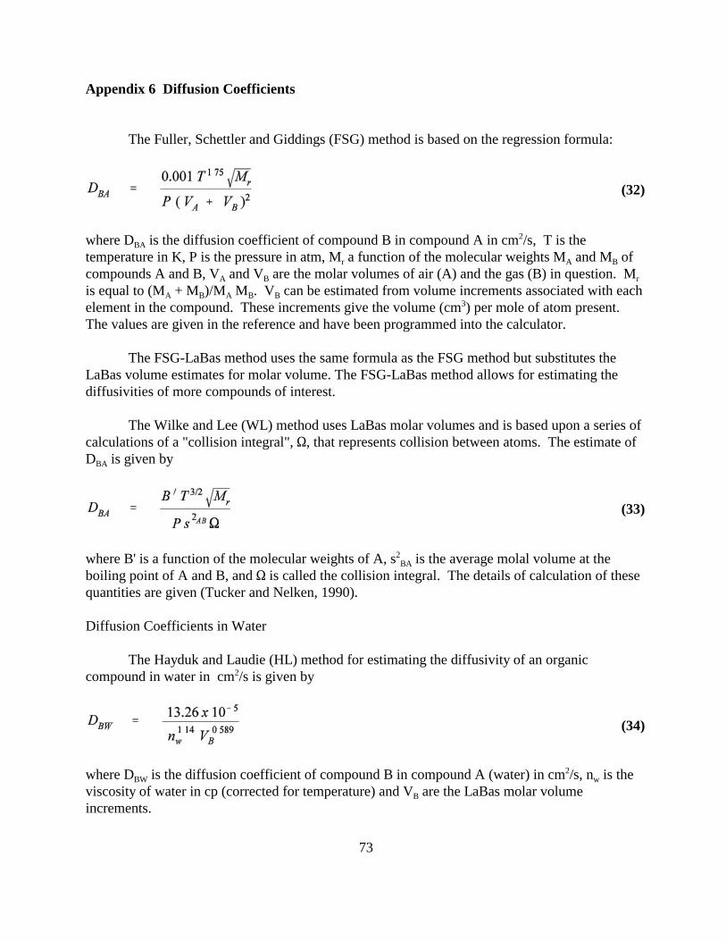
73

Appendix 6 Diffusion Coefficients

The Fuller, Schettler and Giddings (FSG) method is based on the regression formula:

(32)

where DBA is the diffusion coefficient of compound B in compound A in cm2/s, T is thetemperature in K, P is the pressure in atm, Mr a function of the molecular weights MA and MB ofcompounds A and B, VA and VB are the molar volumes of air (A) and the gas (B) in question. Mris equal to (MA + MB)/MA MB. VB can be estimated from volume increments associated with eachelement in the compound. These increments give the volume (cm3) per mole of atom present. The values are given in the reference and have been programmed into the calculator.

The FSG-LaBas method uses the same formula as the FSG method but substitutes theLaBas volume estimates for molar volume. The FSG-LaBas method allows for estimating thediffusivities of more compounds of interest.

The Wilke and Lee (WL) method uses LaBas molar volumes and is based upon a series ofcalculations of a "collision integral", S, that represents collision between atoms. The estimate ofDBA is given by

(33)

where B' is a function of the molecular weights of A, s2BA is the average molal volume at the

boiling point of A and B, and S is called the collision integral. The details of calculation of thesequantities are given (Tucker and Nelken, 1990).

Diffusion Coefficients in Water

The Hayduk and Laudie (HL) method for estimating the diffusivity of an organiccompound in water in cm2/s is given by

(34)

where DBW is the diffusion coefficient of compound B in compound A (water) in cm2/s, nw is theviscosity of water in cp (corrected for temperature) and VB are the LaBas molar volumeincrements.