On-Line Estimation of Inlet and Outlet Composition in Catalytic PartialOxidation

Ali Al-Matouq , Tyrone Vincent

Department of Electrical Engineering and Computer Science, Colorado School of Mines 1600 Illinois St., Golden, CO 80401, USA

Abstract

An estimation strategy is presented for determining inlet and outlet composition of catalytic partial oxidation (CPOX)of methane over rhodium catalyst using simple, fast measurements: temperature, and thermal conductivity. A 1-Dhigh fidelity simulation model for CPOX studied in [1] for a portable fuel cell application is developed and enhancedfor transient experiments. Process dynamics are analysed to demonstrate how solid temperatures along the axes of thereactor reflect the endothermic/exothermic interplay of reactions during a process upset. Model reduction is then usedto obtain a low complexity model suitable for use in a moving horizon estimator with update rates faster than 0.02seconds. System theoretic observability analysis is then conducted to predict the suitability of di↵erent measurementdesigns and the best locations for temperature measurements for estimating both inlet and outlet gas mole fractions forall species. Finally, a Moving Horizon estimator is implemented and simulation experiments are conducted to verifythe accuracy of the estimator.

Keywords: Catalytic Partial Oxidation, Moving Horizon Estimation, Descriptor Systems

1. Introduction

Catalytic partial oxidation reforming of methane is an e�cient process used to produce syngas (H2 and CO) usinga fuel mixture that contains methane CH4 and oxygen O2. CPOX reforming is a compact size low-capital cost reactorthat is suitable for portable applications as in fuel cells. CPOX is also being considered as a potential process for largescale production of syngas in view of its economic and environmental advantages over steam reforming [2].

Fast and accurate measurement of both inlet and outlet gas mole fractions is essential for process reliability andto e↵ectively maintain the quality specifications on syngas. Fuel cells, for example, require varying inlet H2 con-centrations in the stack depending on load demands while maintaining low CO content to avoid poisoning the cell.Furthermore, polymer electrolyte membrane (PEM) fuel cells require low CO2 concentrations. Restrictions on H2Ocontent can also be present. Di↵erent fuel cell and fuel processing control strategies can make use of accurate mea-surements of species mole fractions of the gas coming in and out from the CPOX reactor to enable feed-forwardtemperature control of the reactor, prevent excess H2 generation, prevent fuel cell stack starvation and/or preventCPOX clogging [3], [4].

In this paper an estimator for inferring both inlet and outlet gas mole fractions in real time is developed. Thedeveloped state estimator can be used in portable fuel cell applications for monitoring and/or control. It can also beused in case the main composition measurement device is o↵-line and a substitute is needed to enhance reliability. theestimator design uses a single output measurement, such as thermal conductivity or gas density, that is combined withtemperature measurements along the reactor and nominal input flows. In order to obtain well defined input and outputcomposition estimates, these measurements are reconciled against a reactor model using a moving horizon estimator.

Email address: aalmatou@mines.edu, tvincent@mines.edu (Ali Al-Matouq , Tyrone Vincent)

Preprint submitted to International Journal of H2 Energy February 6, 2014

Previous work towards the development of a nonlinear observer for the CPOX process was given in [5]. A simplelumped parameter model was used that relied on one temperature measurement and one gas species compositionmeasurement at the outlet to infer the remaining outlet gas species compositions at the outlet. The model used,however, was based on only two global reactions; partial and total oxidation and did not account for steam and dryreforming reactions. Further work in [6] was made for estimating inlet gas CH4/O2 ratio in the context of biogasreforming. Also, a simple lumped parameter model of a continually stirred reactor model was used but combined witha detailed reaction mechanism. In both models, spatial variations in temperature along the reactor were not accountedfor, not to mention other important mass and energy transport e↵ects present in the CPOX reforming process.

This paper is an extension of these two studies in multiple directions. First, a high fidelity 1-D model for CPOXprocess, originally studied in [1] and experimentally verified in [7], is developed and enhanced for transient simula-tion experiments. The high fidelity model captures the possible transport and kinetic e↵ects in the lateral direction,assuming homogeneity in the radial and angle coordinates. A detailed analysis of process dynamics is conducted todetermine the important measurements suitable for state estimation. The analysis revealed that solid temperaturesacross the reactor foam monolith have di↵erent dynamics and are highly correlated with the disturbances in the C/Oratio of the inlet gas. The di↵erent temperature dynamics are associated with the exothermic/endothermic interplay ofreactions along the reactor.

Second, several transient simulation experiments with random variations in the inlet C/O ratio were conducted.The collected simulation data was then used to fit a high order state space model using linear subspace identificationtechniques [8]. The resulting high order state space model is then reduced in size using balanced truncation withmatched DC gain. The state space model is then transformed into a descriptor model that is suitable for unknowninput estimation and can incorporate the consistency condition in which the sum of mass fractions in the outlet gasstream must equal to one. A descriptor system observability analysis is performed to evaluate di↵erent measure-ment designs that guarantee numerical stability and uniqueness of the estimates. Local observability analysis of thelow complexity model indicated that three temperature measurements spread apart combined with either a densityor thermal conductivity measurement of the outlet gas stream allows a well conditioned and stable estimator to bedesigned.

Third, a moving horizon state estimator that incorporates the low complexity descriptor model, best measurementdesign, known inequality constraints of the CPOX process is then developed. State estimator performance in terms ofmean square error is then verified via simulation. The estimation accuracy, in terms of mean square error values, wasin the order of O(10�5) with very good performance for inlet gas O2, CH4 and outlet gas H2, CO and Ar species molefractions and marginal accuracy for other variables due to unaccounted non-linearities.

The linearized system identification/model reduction strategy used in this study provided solution times of lessthen 0.02 seconds per iteration which are adequate for the CPOX process time scales but with some compromise inestimation accuracy. Another advantage is that no quasi-steady state assumptions were needed and the time scalesof the original high fidelity model are retained in the low complexity model. Finally, the solution strategy is imple-mentable on a stand alone microprocessor using custom C code generated from CVXGEN available in [9] which canspeed implementation even further.

The organization of the paper is as follows: Section 2 will present the detail model equations of the CPOXreactor used in this study. Section 3 will describe the e↵orts used to accelerate transient simulations of the modelfollowed by an analysis of process dynamics. Section 4 will discuss the process of extracting a low complexity modelusing subspace identification techniques combined with model reduction. Section 5 will formulate the desired stateestimation problem to be solved by forming a descriptor model of the process followed by local observability analysisfor di↵erent proposed measurement designs. Section 6 will present the Moving Horizon State Estimator algorithm fordescriptor systems that will be used and finally Section 7 will present the results obtained followed by a discussion inSection 8.

2. Model Description

The CPOX reformer model adapted in this work was developed in [1] and was also validated via experiments in[7] in the context of biogas fuel reforming. The system consists of a reactor tube made from a catalyst-loaded Al2O3ceramic foam installed inside a furnace as depicted in Figure 1. Feed flows of CH4, O2, and Ar are metered with

2

mass-flow controllers and mixed prior to entering a temperature-controlled tube furnace. The model incorporates adetailed reaction mechanism for methane oxidation over Rhodium using the mechanism studied in [10] and a dustygas model for transport in ↵ Al2O3 foam monoliths. A brief review of the model equations and parameters as given in[1] will be presented first for the convenience of the reader since this model will be used in the subsequent simulationexperiments.

2.1. Model EquationsThe equations for each grid in the 1-D model is first presented. The nomenclature and units used in this study

is summarized in Table 1 for the key variables. The species and mass continuity equations in conservative form aregiven as:

�g@⇢gYi

@t+ rji =(�g!i + As si)Wi, i = 1, · · · ,Kg (1)

�g@⇢g

@t+

KgX

i=1

rji =

KgX

i=1

As siWi (2)

where ⇢g is the gas phase density, �g is foam porosity, Yi is the mass fraction for species i in the gas phase, ji isthe mass flux for species i, !i(Tg) and si(Ts) are the homogeneous and heterogeneous reaction rates evaluated at gasand surface temperatures respectively, Wi is the molecular weight for species i, As is the specific surface area of theactive catalysts (i.e. active surface area per unit volume of foam) and Kg is the number of gas phase species. Sincethe residence time of the reactor is smaller than the gas phase reaction rates, it is possible to neglect the gas phasereactions; i.e. !i ⇡ 0. In the equations, r is used to denote di↵erentiation with respect to the space variable. The massdensity can be determined by the ideal equation of state as follows:

⇢g =p

RTgPKg

i=1 Yi/Wi

(3)

where p is the gas pressure. The mass fluxes ji are determined using the Dusty-Gas model from the following implicitrelationship:

X

l,k

[X`]Ji � [Xi]J`[XT ]De

kl+

Ji

Dek,Kn= �r[Xi] �

[Xi]De

k,Kn� Bg

µr (4)

where Ji is the molar flux of gas phase i, [Xi] is the molar concentration for gas species i, [XT ] = p/RT is the totalmolar concentration of the gas, and Bg is the permeability which may be found for example using the Kozeny-Carman

Figure 1: Process Flow Diagram

3

Variable Description Unit⇢g gas phase density kg.m�3

Yi Mass fraction for species iwi homogeneous reaction rate mole.m�3s�1

si heterogeneous reaction rate mole.m�2.s�1

Wi Molecular weight of species i kg/molep Gas pressure Paji mass flux for gas species i kg.m�2.s�1

Ji molar flux for gas species i mole.m�2.s�1

[Xi] molar concentration for gas species i mole.m�3

Ts Solid phase temperature KTg Gas phase temperature Kqg Heat flux within the gas phase J.m�2.s�1

qs Heat flux within the solid phase J.m�2.s�1

qconv Heat flux due to convection J.m�3.s�1

qsurf Heat flux due to surface reactions J.m�3.s�1

qenv Heat flux due to radiation J.m�3.s�1

e Gas internal energy J.kg�1

cv,i Specific heat capacity at constant volume for species i J.kg�1.K�1

hi Specific gas enthalpy for species i J.kg�1

�g, �s Gas mixture and solid phase thermal conductivity J.m�1.s�1.K�1

hv Volumetric heat transfer coe�cient W.m�3.K�1

µ Gas mixture viscosity kg.m�1.s�1

mg Total gas mass flux kg.m�2.s�1

✓i Surface site coverage for species i

Table 1: Model Nomenclature and Units

relationship referenced in [11] or other empirical techniques relative to the given monolith foam structure. The massflux is then given by ji = WiJi. The mixture viscosity is given as µ and De

kl and Dek,Kn are the e↵ective binary (between

species k and l) and Knudsen di↵usion coe�cients respectively which are found from the following relationships:

Dekl =�g

⌧Dkl, De

k,Kn =43

rp�g

⌧

s

8RTg

⇡Wi(5)

where the definition and values of the parameters ⌧ and rp are given in Table 2. The binary di↵usion coe�cients are de-termined from kinetic theory and can be readily calculated using Cantera [12]. For more details on the implementationof the Dusty gas model, the reader is referred to [11].

The energy balance equations for both the gas phase and the solid phase are respectively given as follows:

�g@⇢ge@t+ rqg = � qconv � qsurf (6)

�s@

@t(⇢scp,sTs) + rqs =qconv + qsurf � qenv (7)

where �s = 1 � �g is the solid phase volume fraction, Ts is the solid temperature, ⇢s is the solid phase density, cp,sis the heat capacity of the solid phase at constant pressure, and qg,qs, qconv, qsurf , qenv are respectively the heat fluxwithin the gas phase, heat flux within the solid phase, heat flux due to convection between the gas and solid phase,heat flux due to surface reactions between the gas and solid phase and heat flux due to radiation between the solidphase and the environment. Finally e is the gas internal energy which can be expressed as e =

PKg

i=1 Yiei. In di↵erential

4

form de =PKg

i=1 Yicv,idTg where cv,i is the specific heat capacity at constant volume for gas species i. Hence, the chainrule may be used to rewrite (6) as:

�g

KgX

i=1

⇢gYicv,i@Tg

@t+ rqg = ��g

KgX

i=1

@⇢gYi

@tei � qconv � qsurf

This modified implementation of equation (6) can make use of (1) which simplifies integration.The gas and solid phase heat fluxes qg,qs are given as:

qg = � �g�grTg +

KgX

i=1

hiji, (8)

qs = � �esrTs (9)

where hi are the species specific enthalpy and �g is gas mixture thermal conductivity; see [12] for mixing rule used,and �e

s is the temperature dependent e↵ective conductivity of the solid phase given by:

�es = �s�s + �r

where �s is the thermal conductivity of the solid and �r is the e↵ective radiation conductivity (due to optically thickporous foam) is found from the following empirical formula [1]:

�r = 4dp�T 3s

n

0.5756✏ tan�1[1.5353(�⇤s )0.8011/✏] + 0.1843o

where �⇤s = �s/(4dp�T 3s ), � is the Stefan-Boltzmann constant, dp is an e↵ective particle diameter and ✏ is the emis-

sivity of the solid material.The convection heat flux qconv is given by:

qconv = hv(Tg � Ts) (10)

where hv = Aconvh is the volumetric heat transfer coe�cient, where h is the conventional heat transfer coe�cientand Aconv is the specific surface area of the porous foam. The value of hv can be obtained from the Nusslet numbercorrelation referenced in [1] as:

Nu =hvd2

p

�g= 2.0 + 1.1Re0.6Pr1/3

where dp is the mean catalyst particle diameter, Re = mgdp/µ is the Reynolds number based on the total gas mass fluxmg =

PKg

i=1 ji and Pr is the Prandtl number given in Table 2.The net heat release rate resulting from heterogeneous surface reactions qsurf is the enthalpy flux rates of gas-phase

species to and from the catalyst surface:

qsurf = �As

X

si<0

siWihi(Tg) � As

X

si�0

siWihi(Ts) (11)

where the convention si < 0 indicates a net gas species flux from the gas toward the surface and vice versa. Thesymbol hi(Tg) denotes enthalpies of the gas phase species evaluated at the gas phase temperature and hi(Ts) denotesenthalpies of the gas phase species evaluated at the solid phase temperature. Note that qsurf was subtracted from (6) asopposed to being added as a source term in (7) due to sign convention.

The radiative heat flux from the foam to the surroundings is given as:

qenv = �✏Aenv(T 4s � T 4

1) (12)

5

Para. Value Description UnitL 2.54 ⇥ 10�2 Reactor length m⌧ 2 Tortuosity of foam monolith�g 0.75 Porosity of foam monolithB 2.52 ⇥ 10�15 Permeability of foamrp 280 ⇥ 10�6 Average pore radius mdp 850 ⇥ 10�6 Particle diameter of foam m✏ 0.5 Emissivity of quartzAenv 337 Interface area of reactor m2

�s 1.4 Quartz Conductivity W.m�1.K�1

As 40,000 Catalyst surface area m�1

D 1.3 ⇥ 10�2 Diameter of the reactor tube mv 3.5 Inlet gas velocity m.s�1

⇢s 3970 Density of quartz kg m�3

cp,s 1225 Specific heat of quartz J.kg�1.K�1

� 2.6 ⇥ 10�9 Active catalyst site density mole.cm�2

Tin 1023 Inlet gas temperature KT1 1073 Furnace temperature KT t=0

s 1073 Initial wall temperature KXin

i 12.4, 6.2, 81.4 Inlet gas mole fraction %CH4, %O2, %ArPin 1 Inlet gas pressure atmPout 0.9996 Outlet gas pressure atmPr 0.7 Prandtl number

Table 2: Model parameters

where Aenv is the interface area of the porous foam and T1 is the surrounding environment temperature of the furnace.The site coverages of surface species ✓i can be obtained from the following balance equation:

d✓idt=

si

�, i = 1, · · · ,Ks (13)

where � is the density of the active catalyst sites on the total surface area of the foam monolith and Ks is the totalnumber of surface species. The consistency conditions in the model are as follows:

KgX

i=1

Yi =1,KsX

i=1

✓i = 1 (14)

The equality constraint for the mass fractions is already embedded in (1) and is shown here to be used later. Thereaction rates are calculated internally within Cantera [12] using the reaction mechanism given in [10] which contains42 elementary reactions, 7 gas species (H2, O2, H2O, CH4, CO, CO2, AR) and 12 surface species (Rh(s), H(s), H2O(s),OH(s), CO(s), CO2(s), CH4(s), CH3(s), CH2(s), CH(s), C(s), O(s)). Moreover, Cantera was used to find the densities,heat capacities, enthalpies, conductivities and viscosities for the gas phase. Details of these calculations can be foundin Cantera documentation available online. Table 2 gives the dimensions and parameters used in the study.

3. Model Simulation and Process Dynamics

3.1. Model SimulationThe partial di↵erential algebraic system of equations are sti↵; i.e. the associated dynamics exhibit both very

short time scales, due to fast heterogeneous reactions, and very long time scales due to heat transfer dynamics. For

6

Figure 2: Simplified Reactor Diagram

steady state simulation the boundary conditions of the model were: constant inlet mass flow rate (set by specifyingthe inlet velocity vin

g and inlet mass fractions Yini ), constant inlet gas temperature T In

g , constant furnace temperatureT1 and constant outlet temperature and pressure of the gas phase, T Out

g , POutg respectively. Figure 2 shows a simplified

diagram with the variables being discussed.The model is one dimensional; i.e. it captures spatial variation in the z-direction only. The system of equations was

discretized in space using second order approximation for the spatial derivatives. A non-uniform mesh was designedusing a logarithmic function with more grids concentrated in the first 0.5 cm of the reactor. The thermodynamic andkinetic calculations were calculated using Matlab Cantera [12]. The combined model equations was then integratedusing Matlab’s sti↵ integrator ”ode15s” [13] using a relative error tolerance of 1⇥10�4 and an absolute error toleranceof 1 ⇥ 10�6. An e↵ort was made to speed up transient simulations by calculating a compressed numerical Jacobianmatrix that exploits sparsity and also by code profiling. Mole fractions are shown in the developed plots instead ofmass fractions for practicality purposes. Figure 3 shows the mole fraction (top) and the solid temperature profilesalong the axes of the reactor at steady state using a non-uniform mesh with 10 grids. These steady state results arecomparable with the results given in [1] for the base line case defined by the values given in Table 2.

3.2. Process DynamicsTransient analysis of start up conditions was given in [14], where the dynamics of total oxidation, partial oxidation

and steam reforming, and their interplay in the di↵erent sections of the reactor was studied. Here, the overall dynamicsof the process when the inlet gas feed is subject to step changes in oxygen and methane during normal operation isanalysed. The overall reactions that compete with each other in the CPOX process are the exothermic partial oxidation,endothermic steam reforming, endothermic dry reforming and exothermic combustion reactions that are globally andrespectively expressed as follows:

CH4 +12 O2 ��! CO + 2 H2, �HR = �36 kJ/mol

CH4 + H2O �! CO + 3 H2, �HR = +206 kJ/molCH4 + CO2 ��! 2 CO + 2 H2, �HR = +247 kJ/molCH4 + 2 O2 ��! CO2 + 2 H2O, �HR = �802 kJ/molIn the simulation study, the feed composition is a mixture of CH4, O2 and Ar only. Figures 4 and 5 depict a

transient simulation experiment where 3 step changes were made to the O2 and CH4 mole fractions. Figure 4 showsthe inlet perturbations (top) and the resulting time response of the solid temperatures across the reactor. Figure 5shows the response of the mole fractions in both the entry and the exit sections of the reactor.

The step changes at t = 1 sec cause a sudden increase in the CH4/O2 ratio from 2 to 2.31 in the inlet gas stream.The associated solid temperature dynamics show a drop in temperatures at the entry portion of the reactor (in thefirst 0.23 cm portion measured from the entry) and a slight increase in temperatures at the remaining portion of the

7

Figure 3: Gas mole fractions and temperature profiles at steady state

reactor (from 0.23 cm to 2.54 cm). The trajectories for the gas mole fractions in Figure 5 (top) show an increase in H2and CO content and a drop in H2O content at the reactor entry associated with this step change. On the other hand,the dynamics near the exit portion of the reactor, also shown in Figure 5 (bottom), shows only a slight increase inH2, CO and H2O content of the gas, but also less CH4 conversion. This suggests that endothermic steam reformingreactions start to increase at the entry potion of the reactor due to the increase in CH4/H2O ratio (from 1.25 to 1.73)producing more H2 and CO. This excess CO, however, will cause more carbon to deposit on the catalyst activesites downstream to form C(s). This can be confirmed by examining Figure 6 which shows the trajectories of thespecies surface coverages. This in turn will free some H2O and O2 generated by surface reactions that will then reactwith the excess CH4 exothermically downstream. Hence, the increase in CH4/O2 ratio from 2 to 2.31 resulted in anunfavourable condition due to less conversion of CH4 and partially deactivating the catalyst.

The step changes at t = 11 sec shows a more drastic increase in the CH4/O2 ratio from 2.31 to 3.13 in the inlet gasstream. The associated solid temperature and mole fraction dynamics suggest an increase in both steam reforming anddry reforming reactions at the entry portion of the reactor. However, near the reactor exit, the transient plots reflecta sharp drop in CH4 conversion, which is expected since severe catalyst deactivation has occurred at this stage asreflected in Figure 6.

The step changes at t = 21 sec shows a decrease in the CH4/O2 ratio from 3.13 to 1.6 in the inlet gas stream. Theassociated solid temperature and mole fraction dynamics suggest the opposite of the previous scenario; an increase inexothermic reactions across the reactor, with a slight increase in endothermic reactions near the exit. At this stage,the catalyst has been reactivated by freeing active sites from C(s) and forming CO and CO2, as suggested in Figures 5

8

Figure 4: Transient simulation experiment: Inlet gas step changes (top) and associated solid temperature dynamics (bottom)

and 6.The above analysis suggests that solid temperature measurements across the reactor can be an indispensable mea-

surement for inferring the inlet gas disturbances and the associated outlet gas mole fractions using the model.

4. Model Simplification and Reduction

4.1. Method JustificationAs demonstrated previously in Section 3, the dynamics of gas compositions, surface coverages and temperatures

exhibit di↵erent time scales. The residence time of the process is in the order of ⇠ 0.01 seconds which furthercomplicates the implementation of real time optimization routines. Moreover, the target application of the CPOXreformer is a portable fuel cell that has cost constraints on the amount of processing power available. Hence, it isimportant to find a real time estimation solution strategy that can provide reasonable estimates of gas compositionsappropriate with the time scales and cost constraints of the process.

The full discritization embedded optimization strategy used in [15], for example, implemented a Moving HorizonNon-linear Programming estimator for a chemical reacting flow problem with 300-400 ODEs which is comparable insize to the CPOX model being used in this study (which consist of 348 ODEs). The quasi-steady state assumptionon the reaction kinetics in [15] was used to resolve model sti↵ness and the method required full discritization usingorthogonal collocation on finite elements for the time variable and Euler approximation on the distance variable.In addition, availability of explicit Jacobian and Hessian model equations and an interior point solver with sparsityinformation was needed to reduce problem complexity. Solution times obtained using this strategy, however, rangedfrom 8.7 seconds to 188 seconds on a personnel computer (depending on the horizon length selected for the MovingHorizon Estimator). The same strategy was also used in [16] for a less complex model with solution times of 30

9

Figure 5: Transient simulation experiment: associated dynamics for the first grid (top) and the last grid (bottom) for gas molefractions

10

Figure 6: Transient simulation experiment: associated dynamics of the species surface coverages at 0.23 cm from the entry

seconds on average using a horizon length of 10 for a control problem. Based on these results, this solution strategywas not used for the CPOX process application in view of the model complexity of the CPOX process, the timeconstraints and implementability restrictions.

Another di↵erent approach was used in [17] for a slow distillation column process that used a multiple shootingstrategy which involved integration of the model in every optimization step. The solution times obtained per iterationusing Moving Horizon Estimation was ⇠ 4 seconds on average. The method, however, relies on the availability of asimulation model that can be integrated rapidly using large time steps, which is possible for process models that donot exhibit sti↵ness.

Hence, a di↵erent solution strategy was used that can be implemented on stand-alone microprocessors and canprovide solution times relevant to the CPOX process time scales with some compromise in estimation performance.The strategy relies on using system identification techniques as a means for simplifying the model while retaining thepredictive capabilities of the full order model. The simplified model is then utilized in fast convex state estimationalgorithms that are implementable on stand-alone microprocessors using custom developed library free C code [9].No quasi-steady state assumptions were used in the high fidelity model in order to capture the time scales accurately inthe reduced model and to make use of the detail reaction mechanism model. This model simplification strategy, eventhough localized to a single operating point, can be extended to multiple operating points using a linear parametervarying model as discussed for example in [18]. The accelerated transient simulation model developed in Section 3permits conducting long experiments required to obtain a linearised model with acceptable accuracy.

4.2. Subspace IdentificationA series of transient simulation experiments were conducted to collect a large set of input/output data at a sample

rate of 0.001 seconds. The inlet methane and oxygen mass fractions were varied using a normally distributed pseudo-random number generator [13], with mean zero and variance of 0.006 added to the nominal mass fractions; 0.0544±0.006 and 0.0545±0.006 (i.e. about 10% variation). Figure 7 shows a portion of the transient simulation experimentsthat were conducted.

The desired input and output variables grouped in vectors uk, yk respectively are defined as follows:

yTk :=[T 1

s,k,T2s,k, · · · ,T `s,k,YOut

H2,k,YOut

O2,k,YOut

H2O,k,YOutCO,k,Y

OutCO2,k,

YOutAR,k, �

Outk ] (15)

uTk :=[Yin

O2,k,Yin

CH4,k], k = 1, 2, · · · ,T (16)

where T `s,k is the solid temperature of the tube reactor at the lth grid at time period k, YOutH2,k

is the mass fraction of H2 inthe outlet gas at time period k. Similarly, Yin

O2,k,Yin

CH4,kare mass fractions of O2 and CH4 in the inlet gas at time period

k respectively. This selection was based on the state estimator problem design considerations which will be discussed

11

later in this study. However, models for other variables in the system; i.e. the internal gas densities ⇢g, the surfacecoverages ✓i, the gas temperatures Tg etc., can be developed using the same methodology presented if desired.

The mean values of the collected input and output data u, y was found and subtracted from uk, yk respectively. Thede-averaged data was then used in the system identification subspace algorithm N4SID studied in [8]. The linear statespace model to be identified and reduced is of the form:

xk+1 =Axk + Buk (17a)yk =Cxk + Duk (17b)

where yk = yk � y, uk = uk � u and xk 2 Rn is the state vector sequence that has no physical meaning. The subspaceidentification problem is defined as: given a set of input/output vector sequences (uk, yk), for k = 1, · · · ,T , estimatethe order of the system n and the system matrices A, B,C,D up to a similarity transform of the state vector sequencexk = T�1xk.

The general steps for subspace identification are discussed here briefly: [19]

1. Regression/Projection: A least squares regression or projection is performed to estimate one or several highorder-models. This step entails forming the input and output Hankel matrices and a projection operator to finda least squares approximation of the observability matrix.

2. Model Reduction: The high order model is then reduced to an appropriate low dimensional subspace that isobservable. This can be achieved using singular value decomposition of the observability matrix with di↵erentpre-weighting techniques to reduce the e↵ect of noise. The canonical variance analysis, studied in [20] wasused in this study.

3. Parameter Estimation (Realization): The reduced order observability matrix is then used to estimate the matricesA, B,C,D which are unique up to a similarity transform of the state vector xk. This can be achieved using matrixdecompositions or least squares minimization methods.

For more details on the assumptions required on the system for open loop sub-space identification and the detailalgorithm the reader is referred to [19].

Separate high order discrete state space models were identified for each individual output; i.e. for each variable inyk. The sample rate was 0.1 seconds. Canonical variate analysis pre-weighting of the observability matrix was used[20]. This resulted in 18 linear state space models that were combined to form one model by stacking together thesystem matrices for the individual models obtained. The resulting model had 18 outputs, 2 inputs and 784 states; i.e.n = 784. To limit the measurement bandwidth, the model was re-sampled so that 1 sec measurements can be usedassuming zero-order hold on the input uk as follows:

xk+10 =A10xk + [A9B + A8B + · · · + B]uk

yk =Cxk + Duk, uk = uk+1 · · · = uk+10

4.3. Model ReductionModel reduction was then performed on this high order linear state space model using balanced truncation with

matched DC gain that discards the states with small Hankel singular values while preserving the DC gain of theoriginal model [21]. The model order was reduced from 784 to 7 states by observing the number of dominant singularvalues and the minimum model order that preserves input/output behaviour. Figure 7 shows a comparison betweenthe simulation of the output resulting from this reduced linear model and the output obtained from simulating theoriginal high fidelity model for both solid temperatures and outlet gas thermo-conductivity. From the shown results,the reduced order linear model exhibits very good performance in the operating region under study, which is su�cientfor the purpose.

5. Problem Formulation and Observability Analysis

5.1. Problem FormulationBefore defining the state estimation problem, some essential variable definitions are first presented. The output

data vector yk given in (15) can be split into two vectors: vector of desired outputs to be estimated yTout,k and the

12

Figure 7: Comparison between reduced order linear model (dashed line) and original first principle model (hard line) for solidtemperature profile and outlet gas thermoconductivity vs. time

measurement vector yTmeas,k defined as follows:

yTout,k :=[YOut

H2,k,YOut

O2,k,YOut

H2O,k,YOutCO,k,Y

OutCO2,k,YOut

AR,k] (18a)

yTmeas,k :=[T 1

s,k,T2s,k, · · · ,T `s,k, �Out

k ] (18b)

The known operating point y is also split as y = [yout, ymeas] according to (18a) and (18b). A noisy detrended mea-surement ymeas,k is defined as follows:

ymeas,k :=ymeas,k � ymeas + vk

where vk represents measurement noise that is assumed to be normally distributed iid random sequence with 0 meanand covariance matrix R; i.e. vk ⇠ N(0,R). An augmented state vector is defined as:

xTk = [xT

k uTk ] (19)

Equation (17b) can be used to write an equation for yout,k as follows:

yout,k = [Cout Dout]xk + yout (20)

where Cout,Dout are the rows of C and D associated with yout,k respectively and yout is the known mean value of theoutlet mass fractions extracted from y. Note: y, u are given from the system identification step explained before anddepend on the operating point.

13

It is desired to design the state estimator such that it can account for possible unmeasured inlet disturbances tothe process. Possible inlet disturbances can be fluctuations in the inlet gas mass fractions, inlet gas temperature andenvironment temperature. All possible disturbances, including disturbances arising from parameter uncertainty, willbe modelled using a normally distributed iid random sequence wk ⇠ N(0,Q) added to (17a) that is independent fromvk. The resulting stochastic linear model of the process and noisy measurements are given as follows:

:=Ez }| {

h

I �Bi

xk+1 =

:=Az }| {

h

A 0i

xk + wk (21a)

ymeas,k =

:=Csmeas

z }| {

h

Cmeas Dmeasi

xk + vk (21b)

The matrices Cmeas,Dmeas are the rows of C and D associated with ymeas,k respectively. The stochastic model composedof (21a) and (21b) is called a stochastic linear descriptor system [22].

It is desired to incorporate the known consistency relationship (14) as an additional deterministic measurement to(21b) by making use of (20) as follows:

0 =

:=ydmeas

z }| {

1 � 1T yout =

:=Cdmeas

z }| {

1T [Cout Dout] xk (22)

where 1T is a vector of ones that e↵ectively acts as a summation operator, ydmeas is a deterministic measurement which

is a constant and Cdmeas is the deterministic measurement matrix. Both (21b) and (22) can be combined in one equation

by forming an augmented measurement vector yk and the resulting process and measurement model will become asfollows:

Exk+1 =Axk + wk (23a)yk =Hxk + vk (23b)

where:

yk =

"

ymeas,kyd

meas

#

, H ="

Csmeas

Cdmeas

#

, vk =

"

vk0

#

, wk = wk

Consequently, if an estimate of the augmented state vector xk is found, an estimate for both uk and yout,k using theknown operating points u, y and (20) can also be found. Hence, the state estimation problem can now be formallystated as follows: Given the measurement vector yk for k = 0, 1, · · · , t, an a priori estimate of the initial state asa random variable x0 ⇠ N(x0, P0) and the stochastic/deterministic model (23a) and (23b) find an estimate of theaugmented state vector sequence xk for k = 0, 1, · · · , t.

5.2. Observability Analysis for the Reduced CPOX Process ModelObservability analysis of descriptor systems of the general form (for both square and rectangular systems) was

studied in [23] using a special Kalman decomposition derived using geometric analysis. Observability ensures thatxk can be found in finite time if the corresponding values of wk, yk are known and the solution is unique (assumingvk = 0). In the context of state estimation, where wk, vk are unknown random sequences that may or may not be zero,system observability ensures convergence to unique unbiased estimates of xk. [22] The following is a useful tool todetermine observability.

Theorem 5.1. (Descriptor System Kalman Decomposition [23])Let E,A 2 Rn⇥n1 , where n < n1 and H 2 Rm⇥n, then there exists non-singular transformation matrices P 2 Rn⇥n andQ 2 Rn1⇥n1 such that:

(PEQ,PAQ,HQ) = "

E11 E120 E22

#

,

"

A11 A120 A22

#

,h

0 H2

i

!

14

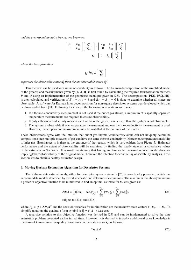
and the corresponding noise free system becomes:"

E11 E120 E22

# "

xnok+1

xok+1

#

=

"

A11 A120 A22

# "

xnok

xok

#

yk =h

0 H2

i

"

xnok

xok

#

where the transformation:

Q�1xk =

"

xnok

xok

#

separates the observable states xok from the un-observable states xno

k .

This theorem can be used to examine observability as follows. The Kalman decomposition of the simplified modelof the process and measurements given by (E,A,H) is first found by calculating the required transformation matricesP and Q using an implementation of the geometric technique given in [23]. The decomposition (PEQ,PAQ,HQ)is then calculated and verification of E11 = A11 = ; and E12 = A12 = ; is done to examine whether all states areobservable. A software for Kalman filter decomposition for non-square descriptor systems was developed which canbe downloaded from [24]. Following these steps, the following observations were made:

1. If a thermo-conductivity measurement is not used at the outlet gas stream, a minimum of 3 spatially separatedtemperature measurements are required to ensure observability.

2. If only a thermo-conductivity measurement of the outlet gas stream is used, than the system is not observable.3. The system is observable if one temperature measurement and one thermo-conductivity measurement is used.

However, the temperature measurement must be installed at the entrance of the reactor.

These observations agree with the intuition that outlet gas thermal-conductivity alone can not uniquely determinecomposition since multiple mixtures of gas can have the same thermo-conductivity. Moreover, temperature sensitivityto inlet gas disturbances is highest at the entrance of the reactor, which is very evident from Figure 5. Estimatorperformance and the extent of observability will be examined by finding the steady state error covariance valuesof the estimates in Section 7. It is worth mentioning that having an observable linearised reduced model does notimply ”global” observability of the original model, however, the intention for conducting observability analysis in thissection was to obtain a healthy estimator design.

6. Moving Horizon Estimation Algorithm for Descriptor Systems

The Kalman state estimation algorithm for descriptor systems given in [25] is now briefly presented, which canaccommodate models described by mixed stochastic and deterministic equations. The maximum likelihood/maximuma posterior objective function to be minimized to find an optimal estimate for xk was given as:

J(xk) =12

(kEx1 � Ax0k2P(⇤)0+

T�1X

k=1

kwkk2Q +T�1X

k=0

kvkk2R), (24)

subject to (23a) and (23b)

where P⇤0 = Q + AP0AT and the decision variables for minimization are the unknown state vectors x1, x2, · · · , xT . Tosimplify notation, the quadratic form symbol kzk2A = zT A�1z was used.

A recursive solution to this objective function was derived in [25] and can be implemented to solve the stateestimation problem presented earlier in real time. However, it is desired to introduce additional prior knowledge inthe form of known linear inequality constraints on the state vector xk as follows:

Fxk d (25)

15

For example, it is known that mass fractions must be a number in the range [0, 1]. Also, it may be known that theinput mass fraction of methane can not exceed a positive number c < 1. These constraints, and other similar ones, canbe represented by (25) by appropriately specifying the matrix F and vector d. This additional prior knowledge can bevery e↵ective in increasing the accuracy of the state estimator [26] [27]. The absence of this information, on the otherhand, can introduce significant errors when the system is operating near the constraints, as demonstrated in [28].

However, if (25) is imposed in the minimization problem (24), a recursive solution to the problem can not beobtained any more. This is because these inequality constraints must be satisfied at all times and the decision variablesin the optimization problem will grow unbounded with t. Moving horizon estimation, MHE, first introduced in [29]for linear state space systems, is a technique to approximately solve the constrained optimization problem (24) and(25) by minimizing over a fixed window in time of size N and ignoring all the cost terms outside this window.An extra cost term is added to the objective function that serves to account for the ignored information outside thewindow. Hence, the size of the minimization problem is fixed and can be solved in real time using quadratic programalgorithms. The constrained moving horizon state estimator problem at the current time k = t enables us to estimatexk for k = t � N, · · · , t and can be stated as follows:

bJmht = min

{xk}tt�N

�mht�N(xt�N) +

t�1X

k=t�N

kwkk2Q +t�1X

k=t�N

kvkk2R

subject to Fxk d, (23a), (23b) (26)

Here, N is the length of the horizon of the moving horizon state estimator which defines the size of the window in pastthat the state estimator explicitly accounts for, �mh

t�N(xt�N) is an extra cost term, which is a function of xt�N , selectedby the designer and only used at times k > N. In loose terms, this extra cost term should be selected such that itsminimization will e↵ectively summarize the knowledge of the ignored data in the past before time k = t � N on thestate estimates at times k = t � N, · · · , t. [30]

The significance of the cost term �mht�N(xt�N) on the stability of the optimal state estimator is emphasized in [31]

and [30] for linear discrete time state space systems. This cost term was related to the arrival cost known in dy-namic programming. Using dynamic programming an analytical expression for the arrival cost for the unconstrainedminimization problem (24) can be derived. Consequently, this arrival cost can be used as the extra cost term in (26)which approximates the true arrival cost. Moreover, this selection of �mh

t�N(xt�N) guarantees stability of the MovingHorizon state estimator. The arrival cost for the unconstrained problem (24) can be derived using the matrix identitiespresented in [25] and is given by:

�mht�N(xt�N) =

12kExt�N � Axmh

t�N�1k2P(�)t�N+ bJt�N�1 (27)

where xmht�N�1 is the optimal estimate obtained from solving the minimization problem (26) at time k = t � N � 1

and bJt�N�1 is the cost of minimizing the unconstrained function (24) which is a number that has no influence onthe solution. Moreover, P(�)

t�N is calculated from the Kalman filter recursions [25] that account for equity constraintsarising from deterministic equations. Algorithm I summarizes the technique used to find the Moving Horizon stateestimate that was applied to the CPOX estimation problem in Section 7. Note, Ker(M) denotes the kernel of matrixM which is an orthobasis spanning the null space of matrix M. The reader is referred to [25] to understand the basisfor these calculations.

7. Results and Discussion

A new transient simulation experiment was conducted to collect data to test the estimator discussed in the previoussection. Random perturbations of magnitude 13% of nominal values were added to the nominal values of oxygen andmethane mass fractions; i.e. 0.0544 ±0.007 and 0.0545±0.007 respectively. In addition, random white noise wasadded to these signals with mean zero and variance 0.005. Three solid temperature measurements positioned at 0.13cm, 0.57 cm and 2.54 cm from the reactor entrance was used. Also a thermo-conductivity measurement installed atthe reactor outlet, as suggested in the previous observability analysis, was included as a measurement. Random whitenoise was added to the measurements obtained from simulation with variance of 5 for solid temperatures and 0.0001

16

Algorithm I: Moving Horizon EstimationInput Data:

E,A,Csmeas,Cd

meas, P0,Q,R, yk, x0, y, u

Initializations:

M = Ker(Cdmeas), P(⇤)

0 = P0, k = 1

Minimization Problem:

min{xk}tt�N

�mht�N(xt�N) +

t�1X

k=t�N

kwkk2Q +t�1X

k=t�N

kvkk2R

subject to Fxk d, and (23a), (23b)

Arrival Cost Recursions:

�mht�N(xt�N) =

12kExt�N � Axmh

t�N�1k2P(�)t�N

P(⇤)t�N =(MT ET P(�)�1

t�N�1EM +MT CsTmeasR

�1CsmeasM)�1

P(�)t�N =AMP(⇤)

t�NMT AT + Q,

P(+)t�N =MP(⇤)

t�NMT

Final Solution:

uestk =u + xest

k (end � 1 : end)yest

out,k =yout + [Cout Dout]xestk , k = 1, · · · ,T

for outlet gas thermal conductivity measurement. Inequality constraints Fxk d were formed to reflect the knowledgeabout the outlet mass fractions being a number between [0, 1] and that the inlet gas mass fractions of methane andoxygen are between [0.038, 0.08]. The covariance matrix for the process noise wk was set as Q = 10�2 ⇥ In+2 whereIn+2 is the identity matrix of size n + 2. The covariance matrix associated with measurement noise vk was set as0.5 ⇥ In for the solid temperature measurements and 10�4 for the thermo-conductivity measurement. Finally, thehorizon length for the Moving Horizon state estimator was set at N = 3.

Algorithm I was implemented using CVX [32] in Matlab [13]. The results using the above information are shownin Figures 8-10 superimposed on the results obtained from transient simulation for comparison. Note that the MHEestimates of inlet mole fractions of both O2 and CH4 and outlet mole fractions of H2, CO, CO2 and Ar showed veryclose resemblance to the outputs coming from the high fidelity model. On the other hand, estimates of outlet gas H2Oand CH4 were marginally accurate due to the inherent non-linearities in these two variables.

The Descriptor Kalman estimate given in [25] was also found and shown in the plots using the symbol (⇤). TheFigures show remarkable results with some exceptions. The mean square error values are shown in Table 3 for boththe Kalman filter and Moving Horizon Estimation algorithms. The associated Symmetric Mean Absolute PercentageError (SMAPE) for each estimated variable was also calculated and shown in Table 3 and is defined as follows [33]:

SMAPE =1t

tX

k=1

�

�

�Xestk � Xsim

k

�

�

�

Xestk + Xsim

k

, (28)

where t is the number of data points, Xestk 2 {XIn,m

O2,k, XIn,m

CH4,k, XOut,m

H2,k, XOut,m

O2,k, XOut,m

H2O,k, XOut,mCO,k , X

Out,mCO2,k, XOut,m

AR,k } denote the es-timated mole fractions, where m=KAL or m=MHE, and Xsim

k = {XInO2,k, XIn

CH4,k, XOut

H2,k, XOut

O2, XOut

H2O,k, XOutCO,k, X

OutCO2,k, XOut

AR,k}denote the corresponding simulated mole fractions.

17

Figure 8: Comparison between estimated results: True Values (hard line), MHE (dashed line), Kalman Filter (*)

Table 3 show relatively large SMAPE values for estimating XOutH2O, XOut

CH4and XOut

CO2. This can be attributed to the

deficiency in the low complexity model in which process non-linearities were not taken into account. Nevertheless,the plots indicate reasonable accuracy even for these variables.

As an indication for the extent of observability, the error covariance for each estimated variable was found fromthe diagonal elements of [Cout Dout]P(+)

ss [Cout Dout]T and the last two diagonal elements of P(+)ss , where P(+)

ss is the steadystate value of P(+)

k given by Algorithm I. The values are also shown in Table 3 that demonstrate good observabilityimplied by the small error covariances.

Table 3 also demonstrates that Moving Horizon Estimation outperformed the Descriptor Kalman Filter in almostall mean square error and SMAPE values. The consistency condition (14) was met exactly in all the solutions obtained.Moreover, the average execution time for each iteration using MHE was 0.0145 seconds on a 2.4 GHz Intel Core i-5desktop computer with 6 GB of 1067 MHz memory. This implementation can also be made roughly 20 times fasterusing custom, library free, C code generated using CVXGEN [9] which can be used on stand-alone microprocessorsif desired. Hence, the execution times obtained are relevant to the time scales and dynamics of the process.

It is worth mentioning however, that using longer horizon lengths; i.e. N > 3, will not result in better estimationaccuracy due to the inevitable model mismatch between the high fidelity model and the reduced model.

Table 4 shows the m.s.e performance for both Kalman filter and MHE when a density measurement is used insteadof a thermal-conductivity measurement at the outlet. This experiment used the same tuning parameters stated beforefor both the error covariances and horizon length and added the same amount of measurement and process noiseas before. The results indicate similar performance as to the previous case indicating that thermal conductivity anddensity measurements at the outlet are interchangeable and provide almost the same amount of observability.

Another test was conducted when neither thermal-conductivity or density measurement is used at the outlet, andonly three solid temperature measurements installed at 0.13 cm, 0.31 cm and 1.88 cm from the inlet. The resultingoverall mean square error performance was 3.1 ⇥ 10�3 for Kalman estimator and 5.1 ⇥ 10�3 for MHE showing thesignificance of thermal-conductivity/density measurement at the outlet in improving estimation performance. Finally,when only two temperature measurements are used (at 0.13 cm and 0.31 cm from the inlet), the descriptor Kalmanestimator provides uninformative estimates with total mean square error of 53.3 due to lack of observability. On the

18

Figure 9: Comparison between estimated results: True Values (hard line), MHE (dashed line), Kalman Filter (*)

other hand, the MHE provided informative estimates with a total mean square error of 1.8 ⇥ 10�3 demonstrating thesignificance of inequality constraints in improving performance of the estimator.

8. Conclusion

A moving horizon estimation strategy for general chemical reacting flow problems applied to the catalytic partialoxidation of methane on rhodium using simulation was presented. The strategy is to use transient simulations of ahigh fidelity chemical reacting flow model to collect desired input/output data for subsequent system identificationand model reduction. The study demonstrated the possibility of inferring both inlet and outlet mole fractions usingonly solid temperature measurements dispersed across the ceramic monolith reactor and one thermal conductivityor density measurement installed at the outlet. Estimator stability was guaranteed by insuring observability. A newMoving Hoirzon Estimation algorithm for descriptor systems was developed with arrival cost calculations that takeinto account deterministic information using the techniques presented in [25].

Although this simulation study was conducted for a CPOX reactor that is typical for small scale applications, theimplications of this work may extend to larger scale applications. However, since the estimator design was tested viasimulation, experimental evidence is still required to confirm the observations in this study.

In the reduced complexity model that was captured, only disturbances in the inlet gas C/O ratio was studiedsince it was found that this variable has the strongest influence on the outlet gas compositions than other unmeasureddisturbances. If desired, the e↵ect of other disturbances; i.e. furnace temperature, gas pressure, gas velocity etc. canbe captured by identifying several sub-models using the same approach presented.

The estimation accuracy of the linear estimator developed in this study, in terms of mean square error values wasin the order of ⇠ O(10�5) with very good performance for estimating inlet O2 and CH4 and outlet H2, CO and Armole fractions. On the other hand, the estimation accuracy achieved for outlet CO2, H2O and CH4 was less successfuldue to model mismatch e↵ects. Improvement of estimation accuracy will be a subject for future studies using directfiltering techniques, as studied for example in [34].

19

Figure 10: Comparison between estimated results: True Values (hard line), MHE (dashed line), Kalman Filter (*)

Acknowledgement

The authors would like to thank Dr. Robert Kee, Dr. Neal Sullivan and Dr. Huayang Zhu of the MechanicalEngineering Department, Colorado School of Mines for all the support and resources they provided that assisted us indeveloping and enhancing the simulation model and for their valuable recommendations for improving this work. Thiswork was partially supported by the Saudi Arabian Ministry of Higher Eduction and ONR grant N00014-12-1-0201.

[1] H. Zhu, R. Kee, J. Engel, D. Wickham, Catalytic partial oxidation of methane using RhSr-and Ni-substituted hexaaluminates, P Combust Inst31 (2) (2007) 1965–1972.

[2] G. Iaquaniello, E. Antonetti, B. Cucchiella, E. Palo, A. Salladini, A. Guarinoni, et al., Natural gas catalytic partial oxidation: A way to syngasand bulk chemicals productiondoi:http://dx.doi.org/10.5772/48708.

[3] J. T. Pukrushpan, A. G. Stefanopoulou, S. Varigonda, L. M. Pedersen, S. Ghosh, H. Peng, Control of natural gas catalytic partial oxidationfor hydrogen generation in fuel cell applications, IEEE T. Contr. Syst. T. 13 (1) (2005) 3–14.

[4] V. Tsourapas, A. G. Stefanopoulou, J. Sun, Model-based control of an integrated fuel cell and fuel processor with exhaust heat recirculation,IEEE T. Contr. Syst. T. 15 (2) (2007) 233–245.

[5] H. Gorgun, M. Arcak, S. Varigonda, S. A. Borto↵, Observer designs for fuel processing reactors in fuel cell power systems, Int. J. HydrogenEnergy 30 (4) (2005) 447–457.

[6] M. J. Kupilik, T. L. Vincent, Estimation of biogas composition in a catalytic reactor via an extended kalman filter, in: IEEE InternationalConference on Control Applications, IEEE, 2011, pp. 768–773.

[7] D. M. Murphy, A. E. Richards, A. M. Colclasure, W. Rosensteel, N. Sullivan, Biogas fuel reforming for solid oxide fuel cells, ECS Trans.35 (1) (2011) 2653–2667.

[8] P. Van Overschee, B. de Moor, Subspace identification for linear systems: theory, implementation, applications, no. v. 1, Kluwer AcademicPublishers, 1996.

[9] J. Mattingley, S. Boyd, Cvxgen: a code generator for embedded convex optimization, Optim. Eng. 13 (1) (2012) 1–27. doi:10.1007/s11081-011-9176-9.URL http://dx.doi.org/10.1007/s11081-011-9176-9

[10] O. Deutschmann, R. Schwiedernoch, L. Maier, D. Chatterjee, Natural Gas Conversion VI: Studies in Surface Sience and Catalysis, Vol. 136,Elsevier, 2001.

[11] H. Zhu, R. J. Kee, V. M. Janardhanan, O. Deutschmann, D. G. Goodwin, Modeling elementary heterogeneous chemistry and electrochemistryin solid-oxide fuel cells, J. Electrochem. Soc. 152 (12) (2005) A2427–A2440.

[12] D. Goodwin, An open-source, extensible software suite for cvd process simulation, Chemical Vapor Deposition XVI and EUROCVD14 (2003) (2003) 08.

20

Table 3: Mean Square Errors with T.C. measurementSpecies Kalman [25] SMAPE% MHE SMAPE% Error Cov.

XInO2

3.0 ⇥ 10�5 3.6 2.3 ⇥ 10�5 2.6 1 ⇥ 10�4

XInCH4

1.64 ⇥ 10�5 2.73 1.28 ⇥ 10�5 2.43 3 ⇥ 10�4

XOutH2

2.38 ⇥ 10�5 1.16 1.63 ⇥ 10�5 0.93 7.6 ⇥ 10�6

XOutO2

0 0 0 0 0XOut

H2O 1.1 ⇥ 10�5 21.3 0.81 ⇥ 10�5 17.0 3.4 ⇥ 10�6

XOutCH4

6.7 ⇥ 10�5 37.6 6.7 ⇥ 10�5 33.7 2.1 ⇥ 10�5

XOutCO 1.0 ⇥ 10�5 1.5 1.1 ⇥ 10�5 1.7 2.6 ⇥ 10�4

XOutCO2

0.76 ⇥ 10�5 20.2 0.5 ⇥ 10�5 12 7.6 ⇥ 10�6

XOutAR 4.9 ⇥ 10�5 0.4 4.2 ⇥ 10�5 0.34 4.3 ⇥ 10�4

overall m.s.e 2.16 ⇥ 10�4 1.85 ⇥ 10�4

Table 4: Mean Square Errors with Density MeasurementSpecies Kalman [25] SMAPE% MHE SMAPE% Error Cov.

XInO2

2.9 ⇥ 10�5 3.4 2.4 ⇥ 10�5 2.6 2.0 ⇥ 10�4

XInCH4

1.8 ⇥ 10�5 2.8 1.3 ⇥ 10�5 2.5 2.0 ⇥ 10�4

XOutH2

2.9 ⇥ 10�5 1.25 2.0 ⇥ 10�5 1.17 5.0 ⇥ 10�6

XOutO2

0 0 0 0XOut

H2O 1.2 ⇥ 10�5 23.7 0.8 ⇥ 10�5 18.3 3.5 ⇥ 10�6

XOutCH4

5.8 ⇥ 10�5 36.8 6.6 ⇥ 10�5 34.5 1.6 ⇥ 10�5

XOutCO 8.1 ⇥ 10�6 1.3 1.1 ⇥ 10�5 1.44 1.5 ⇥ 10�4

XOutCO2

6.9 ⇥ 10�6 23.2 0.52 ⇥ 10�5 11.7 7.2 ⇥ 10�6

XOutAR 4.3 ⇥ 10�5 0.36 5.0 ⇥ 10�5 0.4 2.3 ⇥ 10�4

overall m.s.e 2.04 ⇥ 10�4 2.02 ⇥ 10�4

[13] MATLAB, version 8.0.0.783 (R2012b), The MathWorks Inc., Natick, Massachusetts, 2012.[14] R. Schwiedernoch, S. Tischer, C. Correa, O. Deutschmann, Experimental and numerical study on the transient behavior of partial oxidation

of methane in a catalytic monolith, Chem. Eng. Sci. 58 (3) (2003) 633–642.[15] V. M. Zavala, L. T. Biegler, Optimization-based strategies for the operation of low-density polyethylene tubular reactors: Moving horizon

estimation, Comput. Chem. Eng. 33 (1) (2009) 379 – 390. doi:DOI: 10.1016/j.compchemeng.2008.10.008.[16] L. T. Jacobsen, J. D. Hedengren, Model predictive control with a rigorous model of a solid oxide fuel cell, in: American Control Conference

(ACC), Washington, DC, 2013.[17] P. Kuhl, M. Diehl, T. Kraus, J. P. Schloder, H. G. Bock, A real-time algorithm for moving horizon state and parameter estimation, Comput.

Chem. Eng. 35 (1) (2011) 71–83.[18] R. Toth, Modeling and identification of linear parameter-varying systems, Vol. 403, Springer, 2010.[19] S. Qin, An overview of subspace identification, Comput. Chem. Eng. 30 (10) (2006) 1502–1513.[20] W. Larimore, Canonical variate analysis in identification, filtering, and adaptive control, in: Proceedings of the 29th IEEE Conference on

Decision and Control, IEEE, 1990, pp. 596–604.[21] A. Varga, Balancing free square-root algorithm for computing singular perturbation approximations, in: Proceedings of the 30th IEEE

Conference on Decision and Control, IEEE, 1991, pp. 1062–1065.[22] R. Nikoukhah, A. Willsky, B. Levy, Kalman filtering and riccati equations for descriptor systems, IEEE T. Automat. Contr. 37 (9) (1992)

1325 –1342. doi:10.1109/9.159570.[23] A. Banaszuk, M. Kociecki, F. Lewis, Kalman decomposition for implicit linear systems, IEEE T. Automat. Contr. 37 (10) (1992) 1509–1514.[24] A. Al-Matouq, Kalman decomposition of descriptor systems, 2013.

URL http://www.mathworks.com/matlabcentral/fileexchange/43461-kalman-decomposition-for-descriptor-systems

[25] A. AlMatouq, T. Vincent, L. Tenorio, Reduced complexity kalman filtering of discrete time descriptor systems, in: Proceedings of theAmerican Control Conference, 2013.

[26] D. G. Robertson, J. H. Lee, On the use of constraints in least squares estimation and control, Automatica 38 (7) (2002) 1113 – 1123.doi:10.1016/S0005-1098(02)00029-8.

[27] G. Goodwin, M. Seron, J. Dona, Constrained control and estimation: an optimisation approach, Communications and control engineering,Springer, 2005.

[28] E. L. Haseltine, J. B. Rawlings, Critical evaluation of extended kalman filtering and moving-horizon estimation, Ind. Eng. Chem. Res. 44

21

(2005) 2451–2460.[29] K. R. Muske, J. B. Rawlings, J. Lee, Receding horizon recursive state estimation, in: Proceedings of the American Control Conference, 1993,

pp. 900–904.[30] J. Rawlings, D. Mayne, Model Predictive Control Theory and Design, Nob Hill Pub, Llc, 2009.[31] C. Rao, J. Rawlings, J. Lee, Constrained linear state estimation a moving horizon approach, Automatica 37 (10) (2001) 1619–1628.[32] M. Grant, S. Boyd, Graph implementations for nonsmooth convex programs, in: V. Blondel, S. Boyd, H. Kimura (Eds.), Recent Advances in

Learning and Control, Lecture Notes in Control and Information Sciences, Springer-Verlag Limited, 2008, pp. 95–110.[33] B. E. Flores, A pragmatic view of accuracy measurement in forecasting, Omega 14 (2) (1986) 93–98.[34] L. Fagiano, C. Novara, A combined moving horizon and direct virtual sensor approach for constrained nonlinear estimation, Automatica

49 (1) (2013) 193 – 199. doi:http://dx.doi.org/10.1016/j.automatica.2012.09.009.URL http://www.sciencedirect.com/science/article/pii/S0005109812004700

22