On generalisation and learning:A (condensed) primer on PAC-Bayes

followed byNews from the PAC-Bayes frontline

Benjamin Guedjhttps://bguedj.github.io

7 @bguedj

Chalmers Machine Learning SeminarApril 19, 2021

1 39

Greetings!

Undergrad in pure mathematics, PhD in statistics (2013, SorbonneUniv.) with G. Biau and E. Moulines

Tenured research scientist at Inria since 2014 – Modal team, Lille -Nord Europe

Principal research fellow at UCL since 2018, Dept. of ComputerScience and Centre for AI, and visiting researcher at the AlanTuring Institute

Scientific director of the Inria London Programme since 2020

Research at the crossroads of statistics, probability, machine learning,optimisation.

Statistical learning theory, PAC-Bayes, computational statistics,theoretical analysis of deep learning and representation learning toname but a few interests.

Personal obsession: generalisation.

2 39

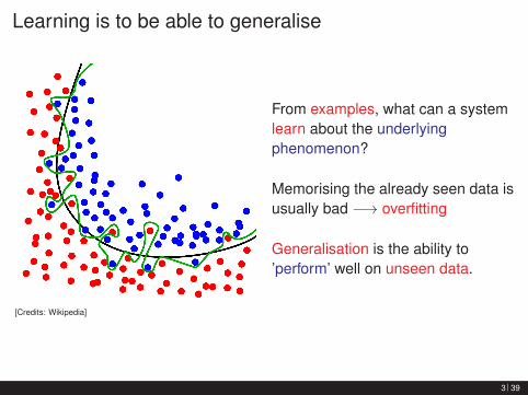
Learning is to be able to generalise

[Credits: Wikipedia]

From examples, what can a systemlearn about the underlyingphenomenon?

Memorising the already seen data isusually bad −→ overfitting

Generalisation is the ability to’perform’ well on unseen data.

3 39

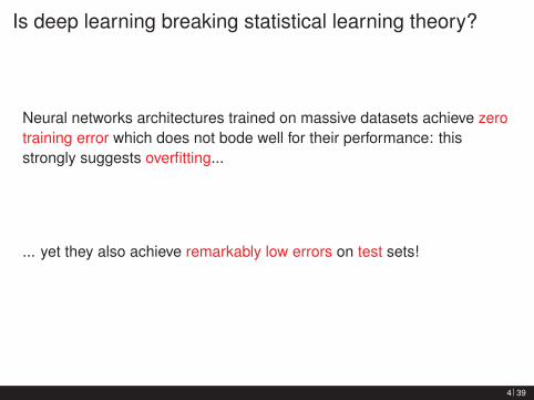
Is deep learning breaking statistical learning theory?

Neural networks architectures trained on massive datasets achieve zerotraining error which does not bode well for their performance: thisstrongly suggests overfitting...

... yet they also achieve remarkably low errors on test sets!

4 39

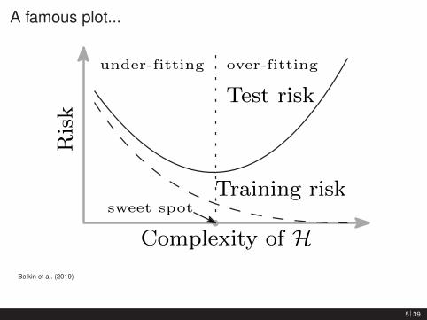
A famous plot...

Risk

Training risk

Test risk

Complexity of Hsweet spot

under-fitting over-fitting

Belkin et al. (2019)

5 39

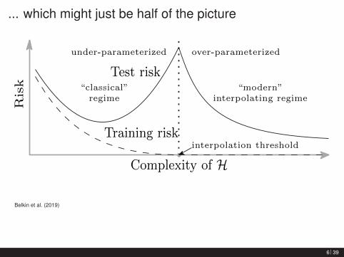
... which might just be half of the pictureRisk

Training risk

Test risk

Complexity of H

under-parameterized

“modern”interpolating regime

interpolation threshold

over-parameterized

“classical”regime

Belkin et al. (2019)

6 39

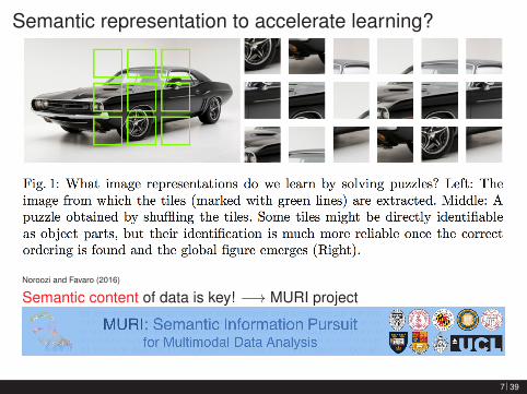
Semantic representation to accelerate learning?

Noroozi and Favaro (2016)

Semantic content of data is key! −→ MURI project

7 39

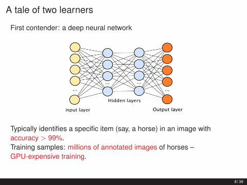
A tale of two learners

First contender: a deep neural network

Typically identifies a specific item (say, a horse) in an image withaccuracy > 99%.Training samples: millions of annotated images of horses –GPU-expensive training.

8 39

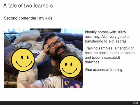
A tale of two learners

Second contender: my kids

Identify horses with 100%accuracy. Also very good attransferring to e.g. zebras

Training samples: a handful ofchildren books, bedtime storiesand (poorly executed)drawings.

Also expensive training.

9 39

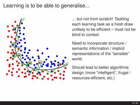
Learning is to be able to generalise...

... but not from scratch! Tacklingeach learning task as a fresh drawunlikely to be efficient – must not beblind to context.

Need to incorporate structure /semantic information / implicitrepresentations of the ”sensible”world.

Should lead to better algorithmsdesign (more ”intelligent”, frugal /resources-efficient, etc.)

10 39

Part IA Primer on PAC-Bayesian Learning

(short version of our ICML 2019 tutorial)

https://bguedj.github.io/icml2019/index.html

11 39

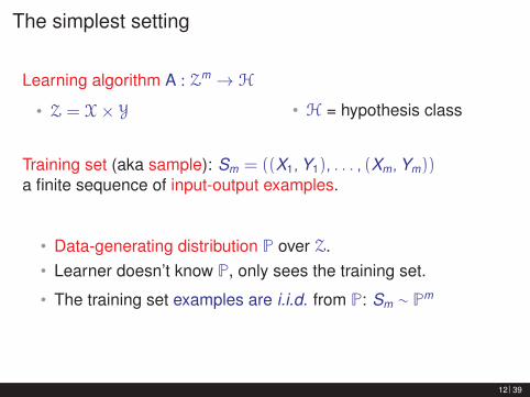
The simplest setting

Learning algorithm A : Zm → H

• Z = X× Y • H = hypothesis class

Training set (aka sample): Sm = ((X1,Y1), . . . , (Xm,Ym))a finite sequence of input-output examples.

• Data-generating distribution P over Z.• Learner doesn’t know P, only sees the training set.

• The training set examples are i.i.d. from P: Sm ∼ Pm

12 39

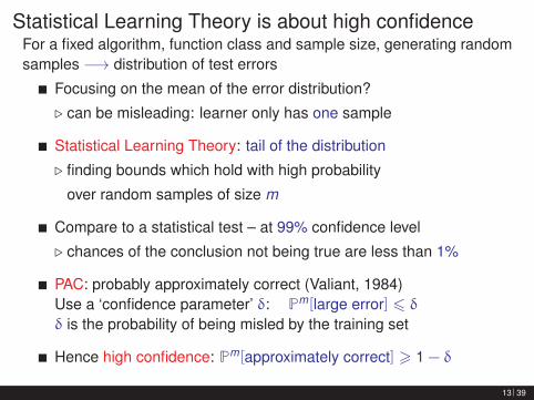
Statistical Learning Theory is about high confidenceFor a fixed algorithm, function class and sample size, generating randomsamples −→ distribution of test errors

Focusing on the mean of the error distribution?

. can be misleading: learner only has one sample

Statistical Learning Theory: tail of the distribution

. finding bounds which hold with high probability

over random samples of size m

Compare to a statistical test – at 99% confidence level

. chances of the conclusion not being true are less than 1%

PAC: probably approximately correct (Valiant, 1984)Use a ‘confidence parameter’ δ: Pm[large error] 6 δδ is the probability of being misled by the training set

Hence high confidence: Pm[approximately correct] > 1 − δ

13 39

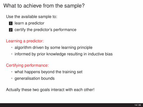
What to achieve from the sample?

Use the available sample to:

1 learn a predictor

2 certify the predictor’s performance

Learning a predictor:

• algorithm driven by some learning principle

• informed by prior knowledge resulting in inductive bias

Certifying performance:

• what happens beyond the training set

• generalisation bounds

Actually these two goals interact with each other!

14 39

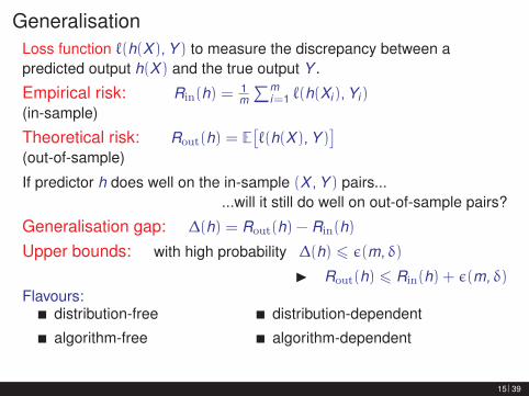
GeneralisationLoss function `(h(X ),Y ) to measure the discrepancy between apredicted output h(X ) and the true output Y .

Empirical risk: Rin(h) = 1m

∑mi=1 `(h(Xi),Yi)

(in-sample)

Theoretical risk: Rout(h) = E[`(h(X ),Y )

](out-of-sample)

If predictor h does well on the in-sample (X ,Y ) pairs......will it still do well on out-of-sample pairs?

Generalisation gap: ∆(h) = Rout(h) − Rin(h)

Upper bounds: with high probability ∆(h) 6 ε(m, δ)

I Rout(h) 6 Rin(h) + ε(m, δ)Flavours:

distribution-free

algorithm-free

distribution-dependent

algorithm-dependent

15 39

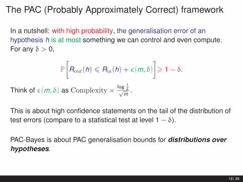
The PAC (Probably Approximately Correct) framework

In a nutshell: with high probability, the generalisation error of anhypothesis h is at most something we can control and even compute.For any δ > 0,

P

[Rout(h) 6 Rin(h) + ε(m, δ)

]> 1 − δ.

Think of ε(m, δ) as Complexity × log 1δ√

m .

This is about high confidence statements on the tail of the distribution oftest errors (compare to a statistical test at level 1 − δ).

PAC-Bayes is about PAC generalisation bounds for distributions overhypotheses.

16 39

Why should I care about generalisation?

Generalisation bounds are a safety check: they give a theoreticalguarantee on the performance of a learning algorithm on any unseendata.

Generalisation bounds:

provide a computable control on the error on any unseen data withprespecified confidence

explain why some specific learning algorithms actually work

and even lead to designing new algorithms which scale to morecomplex settings

17 39

Take-home message

PAC-Bayes is a generic framework to efficiently rethink generalisation fornumerous statistical learning algorithms. It leverages the flexibility of

Bayesian inference and allows to derive new learning algorithms.

ICML 2019 tutorial ”A Primer on PAC-Bayesian Learning”https://bguedj.github.io/icml2019/

Survey in the Journal of the French Mathematical Society: Guedj (2019)

NIPS 2017 workshop ”(Almost) 50 Shades of Bayesian Learning:PAC-Bayesian trends and insights”https://bguedj.github.io/nips2017/

18 39

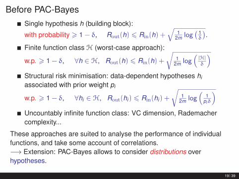
Before PAC-BayesSingle hypothesis h (building block):

with probability > 1 − δ, Rout(h) 6 Rin(h) +√

12m log

( 1δ

).

Finite function class H (worst-case approach):

w.p. > 1 − δ, ∀h ∈ H, Rout(h) 6 Rin(h) +√

12m log

(|H|δ

)Structural risk minimisation: data-dependent hypotheses hi

associated with prior weight pi

w.p. > 1 − δ, ∀hi ∈ H, Rout(hi) 6 Rin(hi) +

√1

2m log(

1piδ

)Uncountably infinite function class: VC dimension, Rademachercomplexity...

These approaches are suited to analyse the performance of individualfunctions, and take some account of correlations.−→ Extension: PAC-Bayes allows to consider distributions overhypotheses.

19 39

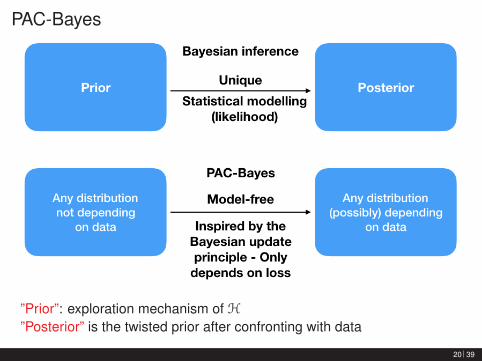
PAC-Bayes

”Prior”: exploration mechanism of H”Posterior” is the twisted prior after confronting with data

20 39

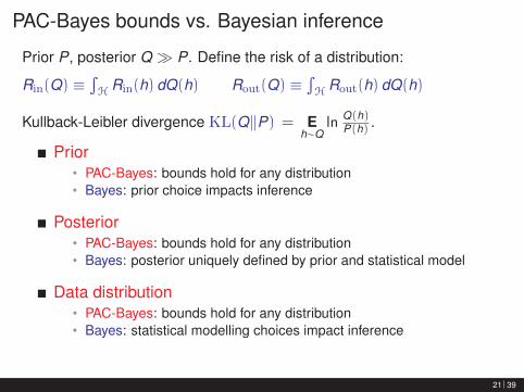
PAC-Bayes bounds vs. Bayesian inference

Prior P, posterior Q � P. Define the risk of a distribution:

Rin(Q) ≡∫H Rin(h) dQ(h) Rout(Q) ≡

∫H Rout(h) dQ(h)

Kullback-Leibler divergence KL(Q‖P) = Eh∼Q

ln Q(h)P(h) .

Prior• PAC-Bayes: bounds hold for any distribution• Bayes: prior choice impacts inference

Posterior• PAC-Bayes: bounds hold for any distribution• Bayes: posterior uniquely defined by prior and statistical model

Data distribution• PAC-Bayes: bounds hold for any distribution• Bayes: statistical modelling choices impact inference

21 39

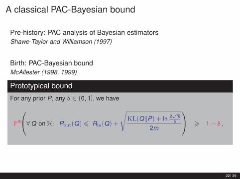
A classical PAC-Bayesian bound

Pre-history: PAC analysis of Bayesian estimatorsShawe-Taylor and Williamson (1997)

Birth: PAC-Bayesian boundMcAllester (1998, 1999)

Prototypical bound

For any prior P, any δ ∈ (0, 1], we have

Pm

∀Q onH : Rout(Q) 6 Rin(Q) +

√KL(Q‖P) + ln 2

√mδ

2m

> 1 − δ ,

22 39

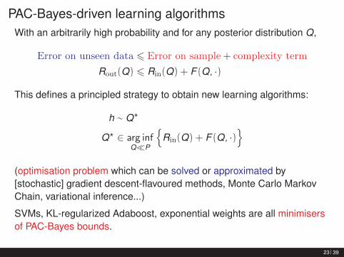
PAC-Bayes-driven learning algorithmsWith an arbitrarily high probability and for any posterior distribution Q,

Error on unseen data 6 Error on sample+ complexity term

Rout(Q) 6 Rin(Q) + F (Q, ·)

This defines a principled strategy to obtain new learning algorithms:

h ∼ Q?

Q? ∈ arg infQ�P

{Rin(Q) + F (Q, ·)

}(optimisation problem which can be solved or approximated by[stochastic] gradient descent-flavoured methods, Monte Carlo MarkovChain, variational inference...)

SVMs, KL-regularized Adaboost, exponential weights are all minimisersof PAC-Bayes bounds.

23 39

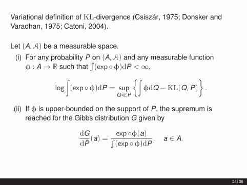
Variational definition of KL-divergence (Csiszar, 1975; Donsker andVaradhan, 1975; Catoni, 2004).

Let (A,A) be a measurable space.

(i) For any probability P on (A,A) and any measurable functionφ : A→ R such that

∫(exp ◦φ)dP <∞,

log

∫(exp ◦φ)dP = sup

Q�P

{∫φdQ −KL(Q,P)

}.

(ii) If φ is upper-bounded on the support of P, the supremum isreached for the Gibbs distribution G given by

dGdP

(a) =exp ◦φ(a)∫(exp ◦φ)dP

, a ∈ A.

24 39

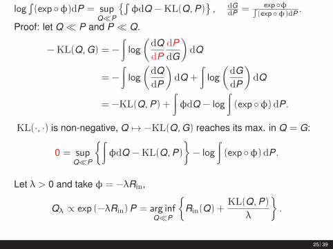
log∫(exp ◦φ)dP = sup

Q�P

{∫φdQ −KL(Q,P)

}, dG

dP = exp◦φ∫(exp◦φ)dP .

Proof: let Q � P and P � Q.

−KL(Q,G) = −

∫log

(dQdP

dPdG

)dQ

= −

∫log

(dQdP

)dQ +

∫log

(dGdP

)dQ

= −KL(Q,P) +

∫φdQ − log

∫(exp ◦φ) dP.

KL(·, ·) is non-negative, Q 7→ −KL(Q,G) reaches its max. in Q = G:

0 = supQ�P

{∫φdQ −KL(Q,P)

}− log

∫(exp ◦φ) dP.

Let λ > 0 and take φ = −λRin,

Qλ ∝ exp (−λRin)P = arg infQ�P

{Rin(Q) +

KL(Q,P)

λ

}.

25 39

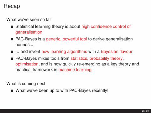
Recap

What we’ve seen so far

Statistical learning theory is about high confidence control ofgeneralisation

PAC-Bayes is a generic, powerful tool to derive generalisationbounds...

... and invent new learning algorithms with a Bayesian flavour

PAC-Bayes mixes tools from statistics, probability theory,optimisation, and is now quickly re-emerging as a key theory andpractical framework in machine learning

What is coming next

What we’ve been up to with PAC-Bayes recently!

26 39

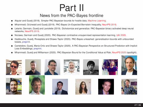
Part IINews from the PAC-Bayes frontline

Alquier and Guedj (2018). Simpler PAC-Bayesian bounds for hostile data, Machine Learning.

Mhammedi, Grunwald and Guedj (2019). PAC-Bayes Un-Expected Bernstein Inequality, NeurIPS 2019.

Letarte, Germain, Guedj and Laviolette (2019). Dichotomize and generalize: PAC-Bayesian binary activated deep neuralnetworks, NeurIPS 2019.

Nozawa, Germain and Guedj (2020). PAC-Bayesian contrastive unsupervised representation learning, UAI 2020.

Haddouche, Guedj, Rivasplata and Shawe-Taylor (2020). PAC-Bayes unleashed: generalisation bounds with unboundedlosses, preprint.

Cantelobre, Guedj, Maria-Ortiz and Shawe-Taylor (2020). A PAC-Bayesian Perspective on Structured Prediction with ImplicitLoss Embeddings, preprint.

Mhammedi, Guedj and Williamson (2020). PAC-Bayesian Bound for the Conditional Value at Risk, NeurIPS 2020 (spotlight).

27 39

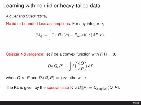
Learning with non-iid or heavy-tailed data

Alquier and Guedj (2018)

No iid or bounded loss assumptions. For any integer q,

Mq :=

∫E (|Rin(h) − Rout(h)|q) dP(h).

Csiszar f -divergence: let f be a convex function with f (1) = 0,

Df (Q,P) =

∫f(dQdP

)dP

when Q � P and Df (Q,P) = +∞ otherwise.

The KL is given by the special case KL(Q‖P) = Dx log(x)(Q,P).

28 39

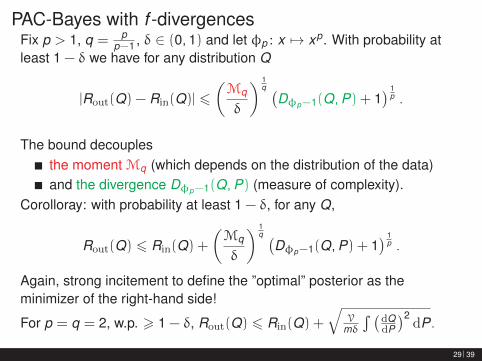
PAC-Bayes with f -divergencesFix p > 1, q = p

p−1 , δ ∈ (0, 1) and let φp : x 7→ xp. With probability atleast 1 − δ we have for any distribution Q

|Rout(Q) − Rin(Q)| 6

(Mq

δ

) 1q (

Dφp−1(Q,P) + 1) 1

p .

The bound decouplesthe moment Mq (which depends on the distribution of the data)and the divergence Dφp−1(Q,P) (measure of complexity).

Corolloray: with probability at least 1 − δ, for any Q,

Rout(Q) 6 Rin(Q) +

(Mq

δ

) 1q (

Dφp−1(Q,P) + 1) 1

p .

Again, strong incitement to define the ”optimal” posterior as theminimizer of the right-hand side!

For p = q = 2, w.p. > 1 − δ, Rout(Q) 6 Rin(Q) +

√V

mδ

∫ (dQdP

)2dP.

29 39

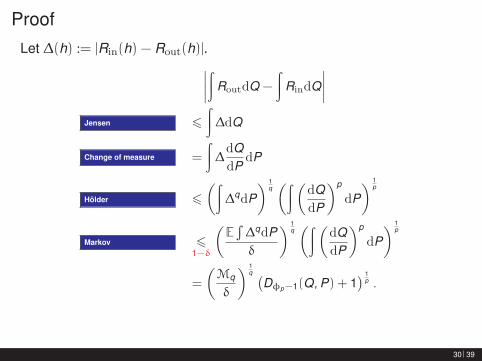
ProofLet ∆(h) := |Rin(h) − Rout(h)|.∣∣∣∣∫ RoutdQ −

∫RindQ

∣∣∣∣Jensen 6

∫∆dQ

Change of measure =

∫∆dQdP

dP

Holder 6

(∫∆qdP

) 1q(∫ (

dQdP

)p

dP) 1

p

Markov 61−δ

(E∫∆qdPδ

) 1q(∫ (

dQdP

)p

dP) 1

p

=

(Mq

δ

) 1q (

Dφp−1(Q,P) + 1) 1

p .

30 39

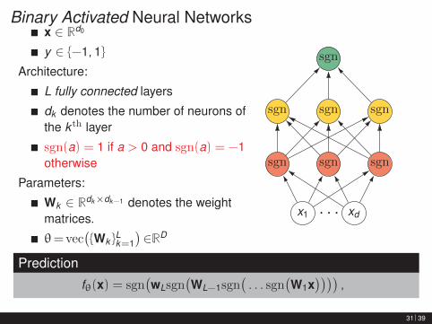
Binary Activated Neural Networksx ∈ Rd0

y ∈ {−1, 1}

Architecture:

L fully connected layers

dk denotes the number of neurons ofthe k th layer

sgn(a) = 1 if a > 0 and sgn(a) = −1otherwise

Parameters:

Wk ∈ Rdk×dk−1 denotes the weightmatrices.

θ= vec({Wk }

Lk=1

)∈RD

x1 · · · xd

sgn sgn sgn

sgn sgn sgn

sgn

Prediction

fθ(x) = sgn(wLsgn

(WL−1sgn

(. . . sgn

(W1x

)))),

31 39

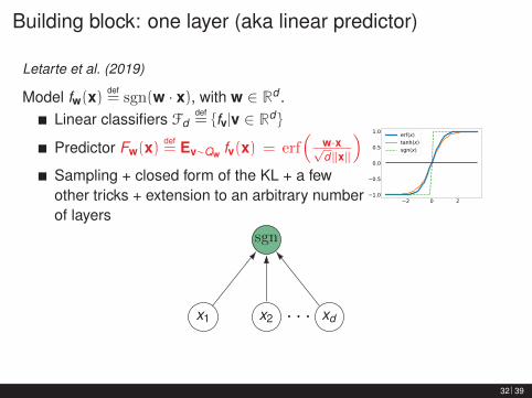
Building block: one layer (aka linear predictor)

Letarte et al. (2019)

Model fw(x)def= sgn(w · x), with w ∈ Rd .

Linear classifiers Fddef= {fv|v ∈ Rd }

Predictor Fw(x)def= Ev∼Qw fv(x) = erf

(w·x√d‖x‖

)Sampling + closed form of the KL + a fewother tricks + extension to an arbitrary numberof layers

2 0 21.0

0.5

0.0

0.5

1.0 erf(x)tanh(x)sgn(x)

x1 x2 · · · xd

sgn

32 39

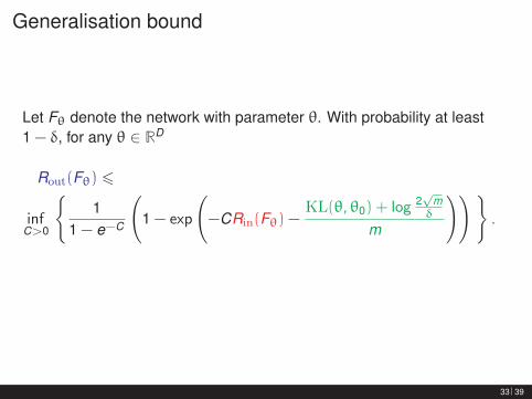
Generalisation bound

Let Fθ denote the network with parameter θ. With probability at least1 − δ, for any θ ∈ RD

Rout(Fθ) 6

infC>0

{1

1 − e−C

(1 − exp

(−CRin(Fθ) −

KL(θ, θ0) + log 2√

mδ

m

)) }.

33 39

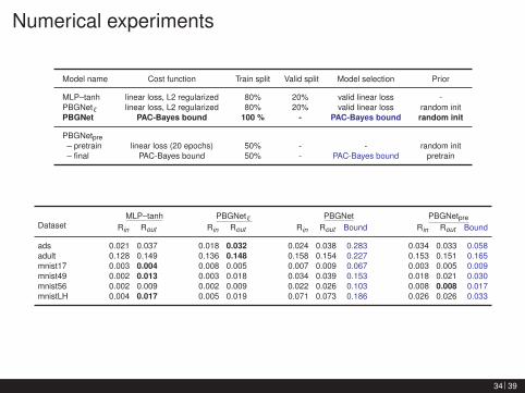
Numerical experiments

Model name Cost function Train split Valid split Model selection Prior

MLP–tanh linear loss, L2 regularized 80% 20% valid linear loss -PBGNet` linear loss, L2 regularized 80% 20% valid linear loss random initPBGNet PAC-Bayes bound 100 % - PAC-Bayes bound random init

PBGNetpre– pretrain linear loss (20 epochs) 50% - - random init– final PAC-Bayes bound 50% - PAC-Bayes bound pretrain

DatasetMLP–tanh PBGNet` PBGNet PBGNetpre

Rin Rout Rin Rout Rin Rout Bound Rin Rout Bound

ads 0.021 0.037 0.018 0.032 0.024 0.038 0.283 0.034 0.033 0.058adult 0.128 0.149 0.136 0.148 0.158 0.154 0.227 0.153 0.151 0.165mnist17 0.003 0.004 0.008 0.005 0.007 0.009 0.067 0.003 0.005 0.009mnist49 0.002 0.013 0.003 0.018 0.034 0.039 0.153 0.018 0.021 0.030mnist56 0.002 0.009 0.002 0.009 0.022 0.026 0.103 0.008 0.008 0.017mnistLH 0.004 0.017 0.005 0.019 0.071 0.073 0.186 0.026 0.026 0.033

34 39

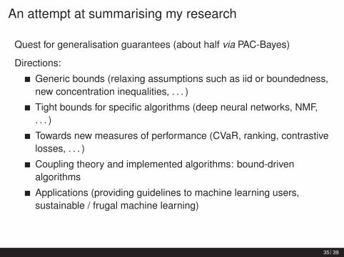
An attempt at summarising my research

Quest for generalisation guarantees (about half via PAC-Bayes)

Directions:

Generic bounds (relaxing assumptions such as iid or boundedness,new concentration inequalities, . . . )

Tight bounds for specific algorithms (deep neural networks, NMF,. . . )

Towards new measures of performance (CVaR, ranking, contrastivelosses, . . . )

Coupling theory and implemented algorithms: bound-drivenalgorithms

Applications (providing guidelines to machine learning users,sustainable / frugal machine learning)

35 39

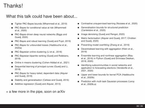
Thanks!

What this talk could have been about...

Tighter PAC-Bayes bounds (Mhammedi et al., 2019)

PAC-Bayes for conditional value at risk (Mhammediet al., 2020)

PAC-Bayes-driven deep neural networks (Biggs andGuedj, 2020)

PAC-Bayes and robust learning (Guedj and Pujol, 2019)

PAC-Bayes for unbounded losses (Haddouche et al.,2020a)

PAC-Bayesian online clustering (Li et al., 2018)

PAC-Bayesian bipartite ranking (Guedj and Robbiano,2018)

Online k -means clustering (Cohen-Addad et al., 2021)

Sequential learning of principal curves (Guedj and Li,2018)

PAC-Bayes for heavy-tailed, dependent data (Alquierand Guedj, 2018)

Stability and generalisation (Celisse and Guedj, 2016)

Additive regression (Guedj and Alquier, 2013)

Contrastive unsupervised learning (Nozawa et al., 2020)

Generalisation bounds for structured prediction(Cantelobre et al., 2020)

Image denoising (Guedj and Rengot, 2020)

Matrix factorisation (Alquier and Guedj, 2017; Chretienand Guedj, 2020)

Preventing model overfitting (Zhang et al., 2019)

Decentralised learning with aggregation (Klein et al.,2019)

Ensemble learning and nonlinear aggregation (Biauet al., 2016) in Python (Guedj and Srinivasa Desikan,2018, 2020)

Identifying subcommunities in social networks andapplication to forecasting elections (Vendeville et al.,2021, 2020)

Upper and lower bounds for kernel PCA (Haddoucheet al., 2020b)

Prediction with multi-task Gaussian processes (Leroyet al., 2020b,a)

+ a few more in the pipe, soon on arXiv

36 39

References IP. Alquier and B. Guedj. An oracle inequality for quasi-Bayesian nonnegative matrix factorization. Mathematical Methods of

Statistics, 26(1):55–67, 2017.

P. Alquier and B. Guedj. Simpler PAC-Bayesian bounds for hostile data. Machine Learning, 107(5):887–902, 2018.

M. Belkin, D. Hsu, S. Ma, and S. Mandal. Reconciling modern machine-learning practice and the classical bias–variance trade-off.Proceedings of the National Academy of Sciences, 116(32):15849–15854, 2019. ISSN 0027-8424. doi:10.1073/pnas.1903070116. URL https://www.pnas.org/content/116/32/15849.

G. Biau, A. Fischer, B. Guedj, and J. D. Malley. Cobra: A combined regression strategy. Journal of Multivariate Analysis, 146:18–28,2016. ISSN 0047-259X. doi: https://doi.org/10.1016/j.jmva.2015.04.007. URLhttp://www.sciencedirect.com/science/article/pii/S0047259X15000950. Special Issue on Statistical Models andMethods for High or Infinite Dimensional Spaces.

F. Biggs and B. Guedj. Differentiable pac-bayes objectives with partially aggregated neural networks. Submitted., 2020. URLhttps://arxiv.org/abs/2006.12228.

T. Cantelobre, B. Guedj, M. Perez-Ortiz, and J. Shawe-Taylor. A pac-bayesian perspective on structured prediction with implicit lossembeddings. Submitted., 2020. URL https://arxiv.org/abs/2012.03780.

O. Catoni. Statistical Learning Theory and Stochastic Optimization. Ecole d’Ete de Probabilites de Saint-Flour 2001. Springer, 2004.

A. Celisse and B. Guedj. Stability revisited: new generalisation bounds for the leave-one-out. arXiv preprint arXiv:1608.06412, 2016.

S. Chretien and B. Guedj. Revisiting clustering as matrix factorisation on the Stiefel manifold. In LOD - The Sixth InternationalConference on Machine Learning, Optimization, and Data Science, 2020. URL https://arxiv.org/abs/1903.04479.

V. Cohen-Addad, B. Guedj, V. Kanade, and G. Rom. Online k-means clustering. In AISTATS, 2021. URLhttps://arxiv.org/abs/1909.06861.

I. Csiszar. I-divergence geometry of probability distributions and minimization problems. Annals of Probability, 3:146–158, 1975.

M. D. Donsker and S. S. Varadhan. Asymptotic evaluation of certain Markov process expectations for large time. Communications onPure and Applied Mathematics, 28, 1975.

B. Guedj. A Primer on PAC-Bayesian Learning. In Proceedings of the second congress of the French Mathematical Society, 2019.URL https://arxiv.org/abs/1901.05353.

B. Guedj and P. Alquier. PAC-Bayesian estimation and prediction in sparse additive models. Electron. J. Statist., 7:264–291, 2013.

37 39

References II

B. Guedj and L. Li. Sequential learning of principal curves: Summarizing data streams on the fly. arXiv preprint arXiv:1805.07418,2018.

B. Guedj and L. Pujol. Still no free lunches: the price to pay for tighter PAC-Bayes bounds. arXiv preprint arXiv:1910.04460, 2019.

B. Guedj and J. Rengot. Non-linear aggregation of filters to improve image denoising. In Computing Conference, 2020. URLhttps://arxiv.org/abs/1904.00865.

B. Guedj and S. Robbiano. PAC-Bayesian high dimensional bipartite ranking. Journal of Statistical Planning and Inference, 196:70 –86, 2018. ISSN 0378-3758.

B. Guedj and B. Srinivasa Desikan. Pycobra: A python toolbox for ensemble learning and visualisation. Journal of Machine LearningResearch, 18(190):1–5, 2018. URL http://jmlr.org/papers/v18/17-228.html.

B. Guedj and B. Srinivasa Desikan. Kernel-based ensemble learning in python. Information, 11(2):63, Jan 2020. ISSN 2078-2489.doi: 10.3390/info11020063. URL http://dx.doi.org/10.3390/info11020063.

M. Haddouche, B. Guedj, O. Rivasplata, and J. Shawe-Taylor. PAC-Bayes unleashed: generalisation bounds with unbounded losses.Submitted., 2020a. URL https://arxiv.org/abs/2006.07279.

M. Haddouche, B. Guedj, O. Rivasplata, and J. Shawe-Taylor. Upper and Lower Bounds on the Performance of Kernel PCA.Submitted., 2020b. URL https://arxiv.org/abs/2012.10369.

J. Klein, M. Albardan, B. Guedj, and O. Colot. Decentralized learning with budgeted network load using gaussian copulas andclassifier ensembles. In ECML-PKDD, Decentralised Machine Learning at the Edge workshop, 2019. arXiv:1804.10028.

A. Leroy, P. Latouche, B. Guedj, and S. Gey. Cluster-specific predictions with multi-task gaussian processes. Submitted., 2020a.URL https://arxiv.org/abs/2011.07866.

A. Leroy, P. Latouche, B. Guedj, and S. Gey. Magma: Inference and prediction with multi-task gaussian processes. Submitted.,2020b. URL https://arxiv.org/abs/2007.10731.

G. Letarte, P. Germain, B. Guedj, and F. Laviolette. Dichotomize and Generalize: PAC-Bayesian Binary Activated Deep NeuralNetworks. arXiv:1905.10259, 2019. To appear at NeurIPS.

L. Li, B. Guedj, and S. Loustau. A quasi-Bayesian perspective to online clustering. Electron. J. Statist., 12(2):3071–3113, 2018.

38 39

References III

D. McAllester. Some PAC-Bayesian theorems. In Proceedings of the International Conference on Computational Learning Theory(COLT), 1998.

D. McAllester. Some PAC-Bayesian theorems. Machine Learning, 37, 1999.

Z. Mhammedi, P. D. Grunwald, and B. Guedj. PAC-Bayes Un-Expected Bernstein Inequality. In NeurIPS 2019, 2019.

Z. Mhammedi, B. Guedj, and R. C. Williamson. PAC-Bayesian Bound for the Conditional Value at Risk. In NeurIPS 2020, 2020. URLhttps://arxiv.org/abs/2006.14763.

M. Noroozi and P. Favaro. Unsupervised learning of visual representations by solving jigsaw puzzles. In European Conference onComputer Vision, pages 69–84. Springer, 2016.

K. Nozawa, P. Germain, and B. Guedj. PAC-Bayesian contrastive unsupervised representation learning. In UAI, 2020. URLhttps://arxiv.org/abs/1910.04464.

J. Shawe-Taylor and R. C. Williamson. A PAC analysis of a Bayes estimator. In Proceedings of the 10th annual conference onComputational Learning Theory, pages 2–9. ACM, 1997. doi: 10.1145/267460.267466.

L. G. Valiant. A theory of the learnable. Communications of the ACM, 27(11):1134–1142, 1984.

A. Vendeville, B. Guedj, and S. Zhou. Voter model with stubborn agents on strongly connected social networks. Submitted., 2020.URL https://arxiv.org/abs/2006.07265.

A. Vendeville, B. Guedj, and S. Zhou. Forecasting elections results via the voter model with stubborn nodes. Applied NetworkScience, 6, 2021. doi: 10.1007/s41109-020-00342-7. URL https://arxiv.org/abs/2009.10627.

J. M. Zhang, M. Harman, B. Guedj, E. T. Barr, and J. Shawe-Taylor. Perturbation validation: A new heuristic to validate machinelearning models. arXiv preprint arXiv:1905.10201, 2019.

39 39