On Dynamic Principal-Agent Problems in Continuous …nwilliam/dynamic-pa1.pdf · On Dynamic Principal-Agent Problems in ... contract by solving a partial differential equation

On Dynamic Principal-AgentProblems in Continuous Time

Noah Williams*

Department of Economics, University of Wisconsin - Madison

E-mail: [email protected]

Revised September 17, 2008

I study the provision of incentives in dynamic moral hazard models with hid-den actions and possibly hidden states. I characterize implementable contractsby establishing the applicability of the first-order approach to contracting. Im-plementable contracts are history dependent, but can be written recursively witha small number of state variables. When the agent’s actions are hidden, but allstates are observed, implementable contracts must take account of the agent’s util-ity process. When the agent has access to states which the principal cannot ob-serve, implementable contracts must also take account of the shadow value (inmarginal utility terms) of the hidden states. As an application of my results, I ex-plicitly solve a model with linear production and exponential utility, showing howallocations are distorted for incentive reasons, and how access to hidden savingsfurther alters allocations.

1. INTRODUCTION

In many economic environments, there arise natural questions as to how to provideincentives in a dynamic setting with hidden information. Some important examples in-clude the design of employment and insurance contracts and the choice of economic pol-icy, specifically unemployment insurance and fiscal policy.1 However the analysis of dy-namic hidden information models rapidly becomes complex, even more so when someof the relevant state variables cannot be monitored. In this paper I develop a tractablemethod to analyze a class of models with hidden actions and hidden states.

I study the design of optimal contracts in a dynamic principal-agent setting. I con-sider situations in which the principal cannot observe the agent’s actions, and the agentmay have access to a privately observable state variable as well. One of the main diffi-culties in analyzing such models is in incorporating the agent’s incentive compatibilityconstraints. Related issues arise in static principal-agent problems, where the main sim-plifying method is the first-order approach. This method replaces the incentive compat-ibility constraints by the first order necessary conditions from the agent’s decision prob-

* I thank Dilip Abreu, Jaksa Cvitanic, Narayana Kocherlakota, Nicola Pavoni, Chris Phelan, Yuliy Sannikov, IvanWerning, and Xun Yu Zhou for helpful comments. I also especially thank Bernard Salanie (the editor) and two anony-mous referees for comments that greatly improved the paper.

1 The list of references here is long and expanding. A short list of papers related to my approach or setting include:Holmstrom and Milgrom (1987), Schattler and Sung (1993), Sung (1997), Fudenberg, Holmstrom, and Milgrom (1990),Rogerson (1985a), Hopenhayn and Nicolini (1997), and Golosov, Kocherlakota, and Tsyvinski (2003).

1

2 NOAH WILLIAMS

lem. Hence the problem becomes solvable with standard Lagrangian methods. Howeverit has been known at least since Mirrlees (1999) (originally 1975), that this approach is notgenerally valid. Different conditions insuring the validity of the first-order approach ina static setting have been given by Mirrlees (1999), Rogerson (1985b), and Jewitt (1988).But there has been little previously work on the first-order approach in a dynamic set-ting, which has hindered the analysis of such models. Working in continuous time, Iestablish the validity of the first-order approach in a very general dynamic model.2

When only the agent’s actions are hidden, under mild conditions the first-order ap-proach gives a complete characterization of the class of implementable contracts, thosein which the agent carries out the principal’s recommended action. Even in the staticsetting, the conditions insuring the validity of the first order approach can be difficult tosatisfy, and they become even more complex in more than one dimension. By contrastmy conditions are quite natural, are easily stated in terms of the primitives of the model,and apply to multidimensional settings. I simply require that effort increase output butdecrease utility, and that output and utility each be concave in effort. Thus my resultshere are quite general, and easier to apply than even in static settings. I discuss the rea-sons for this below, and show how my results relate to the static moral hazard literature.

When the agent has access to hidden states as well, I show that the first-order ap-proach is valid under stronger concavity assumptions. As I discuss below, these assump-tions are too strong for some typical formulations with hidden savings, although theymay apply in other hidden state models.3 Nevertheless, even when the sufficient con-ditions fail, the first-order approach can be used to derive a candidate optimal contract.Then one can check whether the contract does indeed provide the proper incentives.4

To illustrate my methods, I study a more fully dynamic extension of Holmstrom andMilgrom (1987) in which the principal and agent have exponential preferences, and pro-duce and save via linear technologies. In this setting I explicitly solve for the optimalcontracts under full information, when the agent’s effort action is hidden, and when theagent has access to hidden savings as well. I characterize how the informational fric-tions distort the labor/leisure margin (a “labor wedge”) and the consumption/savingsmargin (an “intertemporal wedge”).5 Moral hazard in production leads directly to awedge between the agent’s marginal rate of substitution and the marginal product of la-

2 Independently in concurrent research, Sannikov (2008) has given a similar proof in a simpler model with onlyhidden actions. More recently (after earlier drafts of this paper), Westerfield (2006) analyzes a related model usingdifferent techniques, and Cvitanic, Wan, and Zhang (2006) analyze hidden action models with only terminal payments.But there are no comparable results of my generality, and none of these papers touch on the hidden action case. Thereare some related results on the first-order approach in other dynamic settings. For example, Phelan and Stacchetti(2001) use a first-order approach to characterize optimal Ramsey taxation.

3 See Allen (1985), Cole and Kocherlakota (2001), Werning (2002), Abraham and Pavoni (2008), Kocherlakota (2004a),and Doepke and Townsend (2006) for some alternative formulations with hidden savings. In Williams (2008), I showthat the methods developed here can be used to characterize models with persistent private information.

4Werning (2002) and Abraham and Pavoni (2008) follow similar procedures to numerically check whether the candi-date optimal contract is implementable. In section 7 below, I do so analytically. Kocherlakota (2004a) explicitly solvesa particular hidden savings model using different means and provides a discussion.

5 See Chari, Kehoe, and McGrattan (2007) on the role of the labor and intertemporal (or investment) wedges influctuations. Kocherlakota (2004b) shows how intertemporal wedges result form dynamic moral hazard problems.

ON DYNAMIC PRINCIPAL-AGENT PROBLEMS IN CONTINUOUS TIME 3

bor. Moreover, the dynamic nature of the contracting problem leads to a wedge betweenthe agent’s intertemporal marginal rate of substitution and the marginal product of cap-ital. If the principal can control the agent’s consumption (or tax his savings), the contractwill thus have an intertemporal wedge. However with hidden savings, the agent’s con-sumption cannot be directly controlled by the principal. Thus there is no intertemporalwedge, but instead a larger labor wedge. Finally, I show how the contracts can be imple-mented by a history-dependent, performance-related payment and a tax on savings.

My analysis builds on and extends Holmstrom and Milgrom (1987) and Schattler andSung (1993), who studied incentive provision in a continuous time model. In those pa-pers, the principal and the agent contract over a period of time, with the contract speci-fying a one-time salary payment at the end of the contract period. In contrast to these in-tertemporal models, which consider dynamic processes but only a single transfer from theprincipal to the agent, in my fully dynamic model transfers occur continuously through-out the contract period.6 In such a dynamic setting, the agent’s utility process becomesan additional state variable which the principal must respect. This form of history depen-dence is analogous to many related results in the literature, starting with Abreu, Pearce,and Stacchetti (1986)-(1990) and Spear and Srivastrava (1987).

As noted above, the paper closest to mine is Sannikov (2008), who studies a modelwith hidden actions and no state variables other than the utility process. While there aresimilarities in some of our results, there is a difference in focus. Sannikov’s simpler setupallows for more complete characterization of the optimal contract. In contrast my resultscover much more general models with natural dynamics and with hidden states, but thegenerality implies that typically I can only provide partial characterizations. However, Ido show how to use my methods to solve for optimal contracts in particular settings.

When the agent has access to hidden states, the principal must respect an additionalstate variable which summarizes the “shadow value” of the state in marginal utilityterms. My results, which draw on some results in control theory due to Zhou (1996),are similar to the approach of Werning (2002) and Abraham and Pavoni (2008) in dis-crete time dynamic moral hazard problems. While I’m able to provide some conditionsto prove the validity of the first-order approach ex-ante (which the discrete time literaturehas not), the conditions are rather stringent and thus in many cases I too must check im-plementability ex-post (like Werning and Abraham and Pavoni). However even in suchcases, the continuous time methods here may have some computational advantages, aswe can find an optimal contract by solving a partial differential equation. Section 7 pro-vides one case where this can be done analytically.

An alternative approach is considered by Doepke and Townsend (2006), who developa recursive approach to hidden states models by enlarging the state space. In their setupthe state vector includes the agent’s promised utility conditional on each value of theunobserved state. This requires discretization of the state space, and leads to a large

6 The recent paper by Cadenillas, Cvitanic, and Zapatero (2005) studies a general intertemporal model with fullobservation, and some of their results cover dynamic transfers. Detemple, Govindaraj, and Loewenstein (2005) extendthe Holmstrom and Milgrom (1987) model to allow hidden states.

4 NOAH WILLIAMS

number of incentive constraints which need to be checked. While they provide someways to deal with these problems, their results remain less efficient than mine, albeitrequiring some less stringent assumptions.

2. OVERVIEW

In order to describe the main ideas and results of the paper, in this section I describe asimple version of a benchmark the dynamic moral hazard model. I then summarize themain results of the paper, and relate them to the literature. I defer formal detail to latersections, which also consider more general settings.

2.1. A moral hazard model: hidden actions

The model is set in continuous time, with a principal contracting with an agent overa finite horizon [0, T ]. Output yt is determined by the effort et put forth by the agent aswell as Brownian motion shocks Wt. In particular:

dyt = f(et)dt + σdWt, (1)

where the f is twice differentiable with f ′ > 0, f ′′ < 0. Later sections allow for morecomplex specifications, as current output is allowed to depend on time, its own pastvalues, current consumption or payments, and other state variables. As in the classicmoral hazard literature, I focus here on the case where output is the sole state variableand it is observed by the principal, while he cannot distinguish between effort and shockrealizations. Later I discuss cases when the agent observes some states that the principalcannot. The principal designs a contract that provides the agent consumption st andrecommends an effort level et. The agent seeks to maximize his expected utility:

E

[∫ T

0

u(st, et)dt + v(sT )

], (2)

where u is twice differentiable with ue < 0, uee < 0. Later I consider more generalpreferences, allowing time dependence (for discounting) as well state dependence.

In section 4, I apply a stochastic maximum principle due to Bismut (1973) to charac-terize the agent’s optimality conditions facing a specified contract.7 Similar to the de-terministic Pontryagin maximum principle, the stochastic maximum principle defines aHamiltonian, expresses optimality conditions as differentials of it, and derives “co-state”or adjoint variables. Here the Hamiltonian is:

H(e) = γf(e) + u(s, e), (3)

7 The basic maximum principle is further exposited in Bismut (1978). More recent contributions are detailed inYong and Zhou (1999). Bismut (1975) and Brock and Magill (1979) give early important applications of the stochasticmaximum principle in economics.


See equation (16) below for the more general case. The agent’s optimal effort choice e∗ isgiven by the first order condition:

γf ′(e∗) = −ue(s, e∗), (4)

where equation (20) below provides the more general case.From the literature starting with Abreu, Pearce, and Stacchetti (1986)-(1990) and Spear

and Srivastrava (1987), we know that in a dynamic moral hazard setting a contractshould condition on the agent’s promised utility. Here the promised utility process qt

plays the role of a co-state. In particular, the co-state follows:

dqt = −u(st, e∗t )dt + γtσdWt, qT = v(sT ). (5)

This follows from the more general (17) below, and its solution can be expressed:

qt = E

[∫ T

t

u(st, e∗t )dt + v(sT )

∣∣∣∣Ft

].

Thus qt is the agent’s optimal utility process, the remaining expected utility at date t whenfollowing an optimal control e∗. Here γt gives the sensitivity of the agent’s promisedutility to the fundamental shocks, and is the key for providing incentives. Note from (4)that under our assumptions on u and f we see that γ > 0. Therefore the agent’s promisedutility increases with positive shocks (positive movements in Wt).

One of the main results of the paper, Proposition 5.1, establishes that the first-order ap-proach to contracting is valid in this environment. In particular, I show that if a contractst, et is consistent with the evolution of (5) —a “promise-keeping” constraint —whereγt = −ue(st, et)/f

′(et) from (4) —a local incentive compatibility constraint —then thecontract is implementable. That is, the agent will in find it optimal to choose et when fac-ing the contract. Moreover all implementable contracts can be written in this way, andthe results hold for much broader specifications than outlined in this section. The keyrestrictions are the natural monotonicity and concavity assumptions on preferences andproduction. As mentioned in the introduction, this result is far stronger than what hasbeen shown in discrete time or even in static settings. I next try to provide some intuitionas to why the results are so strong here.

2.2. Relation with previous results2.2.1. Sufficient conditions for the first-order approach in static models

As discussed in the introduction, it is well-known that the first-order approach onlyholds in a static environment under rather stringent conditions, as spelled out by Mir-rlees (1999), Rogerson (1985b), and Jewitt (1988). However these conditions are mucheasier to satisfy when an action by the agent has a (vanishingly) small effect on distribu-tion of output.8 For this argument, I embed a static model in a dynamic framework. In

8For contemporary discussions of the first-order approach in static models, see chapter 4 of Bolton and Dewatripont(2005). The argument in this section was suggested by Bernard Salanie, the editor.

6 NOAH WILLIAMS

particular, let T = 1 and suppose that effort is constant at e0 over the interval [0, 1]. Thenoutput at date 1 is given by:

y1 = f(e0) + W1.

Apart from the timing, this is a static model where W1 is a standard normal shock withdensity φ, thus output has the density φ(y − f(e)) and the normal distribution functionΦ(y − f(e)). The sufficient conditions for the first order approach are the monotone-likelihood ration property (MLRP) and the convexity of the distribution function con-dition (CDFC). In this setting the MLRP holds under the natural assumption that theproduction function is strictly increasing:

d

dy

[φe(y − f(e))

φ(y − f(e))

]= f ′(e) > 0.

However the CDFC can’t be assured, as we have:

Φee(y − f(e)) = φ′(y − f(e))f ′(e)2 − φ(y − f(e))f ′′(e).

As Jewitt (1988) notes, if f(e) = e then the CDFC only holds (Φee ≥ 0) if the density φ isincreasing everywhere (φ′ ≥ 0), which clearly is not the case for the normal density. Incases like this it is difficult to guarantee in advance that the first-order approach is valid.

Now divide the time interval [0, 1] into N different sub-intervals of length ∆ and sup-pose that the agent may choose different effort levels for each sub-interval. In this case,output is given by:

y1 =N−1∑i=0

f(e∆i)∆ + W1.

This is a discretized (and integrated) version of equation (1) with σ = 1. For each choiceet, t ∈ 0, ∆, · · · , (N − 1)∆ = T we now show that the sufficient conditions hold forsmall enough ∆. The MLRP continues to hold for all ∆, as we have:

d

dy

φet

(y −∑N−1

i=0 f(e∆i)∆)

φ(y −∑N−1

i=0 f(e∆i)∆)

= f ′(et)∆ > 0.

But now for the CDFC we have:

Φetet

(y −

N−1∑i=0

f(e∆i)∆

)= φ′

(y −

N−1∑i=0

f(e∆i)∆

)f ′(et)

2∆2−φ

(y −

N−1∑i=0

f(e∆i)∆

)f ′′(et)∆.

While this can’t be guaranteed to be positive in general, for small enough ∆ the secondterm dominates, and so the CDFC will hold if f is concave.

Thus by passing to the limit in which the agent takes frequent actions, with each actionhaving a diminishingly small effect on the distribution of output, we can insure that thefirst-order approach is valid. The first-order conditions use only local information, and


when an action is relevant for a very short horizon such information is sufficient. Thispaper shows that this logic extends to much more general dynamic environments.

2.2.2. Models with two performance outcomes

While the preceding argument is informative, the argument in this paper is fairly dif-ferent, and has similarities with simpler static models where output can take on onlytwo values.9 In particular, a key step in my analysis uses the fact that we can express theagent’s utility under the contract with a target effort policy et as:

∫ T

0

u(st, et)dt + v(sT ) = Ee

[∫ T

0

u(st, et)dt + v(sT )

]+ VT

where Ee[VT ] = 0, and where the expectations are conditional on employing et. Thissimply states that the realized utility is equal to expected utility plus a mean zero shock.Due to the special structure of the Brownian information flow, we can further express the“utility shock” VT as a stochastic integral:

VT =

∫ T

0

γtdWt =

∫ T

0

γt(dyt − f(et)dt), (6)

for some process γt.10 This representation is what allows me to depict the utility pro-cess as in (5) above, and to tie the utility sensitivity γt to the optimality conditions.

Similar results hold in a static model, again with effort fixed at e0 on the interval[0, 1]. For this argument, it is convenient to work with separable preferences, so assumeu(st, et) = u(et). Then we can write:

u(e0) + v(s1) = E[u(e0) + v(s1(y1))|e0] + V1(y1),

where we emphasize that V1 and s1 are dependent on the realization of y1, and E[V1|e0] =0. For an arbitrary output distribution we cannot say much more. But now suppose thaty1 = 1 with probability f(e0) and y1 = 0 with probability 1 − f(e0), where we of courseassume 0 ≤ f(e) ≤ 1.11 In this case it is easy to verify that we can express the ”utilityshock” in a way similar to (6):

V1(y1) = γ(y1 − f(e0)),

where the sensitivity term γ is the difference in the utility of consumption across outputrealizations: γ = v(s1(1)) − v(s1(0)). With this representation, we can then write theagent’s problem given a contract as:

maxe

E[u(e) + v(s1(y1))|e] = maxe

u(e) + v(s1)− γ(y1 − f(e)).

The first order condition for the optimal effort choice is:

γf ′(e∗) = −u′(e∗),

9The discussion of two performance outcome models follows chapter 4.1 of Bolton and Dewatripont (2005).10See Theorem 4.15 and Problem 4.17 in Karatzas and Shreve (1991), which also state the required conditions.11Moreover, to obtain an interior solution we assume that f(0) = 0, lime→∞ f(e) = 1, and f ′(0) > 1.

8 NOAH WILLIAMS

which is directly parallel to (4), the first-order condition in the dynamic model. In addi-tion, this first-order condition is sufficient when f ′′ < 0 and u′′ < 0, the same conditionsas in my dynamic setting.

While the ease of analysis of the static two outcome case has been known, it is strik-ing to see how much of it carries over to more complex dynamic environments.12 Eventhough the diffusion setting of my dynamic model has a continuum of outcomes, andthere may be general temporal dependence in output, the key local properties are simi-lar to this static binary model with i.i.d. shocks.

2.3. A more complex case: hidden statesWhile thus far I have discussed models in which all states are observed, I also consider

a more complicated environment in which the agent has access to a hidden state variable.In such situations, a recursive representation of the contract needs to condition on some-thing more than just the promised utility. I use a first-order approach to show that, atleast in some cases, it is sufficient to condition on the “shadow value” of the hidden statein marginal utility terms.

In particular, suppose that the agent’s consumption ct cannot be observed, and that itinfluences the evolution of a hidden state mt, which evolves as:

dmt = b(mt, st, ct)dt.

The agent’s preferences are as in (2), but now with ct replacing st and terminal utilityv(cT ,mT ). My motivating example is a model of hidden savings which has:

dmt = (rmt + st − ct)dt, (7)

where mt is the agent’s hidden wealth, which earns a constant rate of return r, gets in-flows due to the payment st from the principal, and has outflows for consumption. Themore general specification of b also captures the persistent private information specifica-tion in Williams (2008), where m is the cumulation of the agent’s past misreports of hisprivately observed income. More general cases are considered in (12) below.

With the hidden state, the agent’s Hamiltonian now becomes:

H(m, e, c) = (γ + Qm)f(e) + pb(m, s, c) + u(c, e). (8)

Optimizing (8) by choice of c yields:

−bc(m, s, c∗)p = uc(e∗, c∗). (9)

While γ is once again the sensitivity of the utility process (5), p is a second co-state vari-able and Q is its sensitivity:

dpt = −bm(mt, st, ct)ptdt + QtσdWt, pT = vm(cT ,mT ). (10)

See equation (18) below for the more general case.

12Similar binomial approximations have been widely used in asset pricing (see Cox, Ross, and Rubinstein (1979) foran influential example), and Hellwig and Schmidt (2002) study such approximations in a setting like mine.


The interpretation of pt is most apparent in the hidden savings model (7). In that casebc = −1 and thus (9) shows that p is the marginal utility of consumption. Moreover sincebm = r, the solution to (10) can be written:

pt = E[er(T−t)vm(cT ,mT )

∣∣Ft

].

By the law of iterated expectations, this implies that an Euler equation holds, as for s > t:

uc(ct, et) = E[er(s−t)uc(cs, es)

∣∣Ft

].

The agent’s optimality conditions pin down the expected evolution of the marginal util-ity of consumption, while the contract influences the volatility of marginal utility Qt.

The paper’s main result with hidden states, Proposition 5.2, provides necessary andsufficient conditions for the first-order approach to be valid in this environment. In par-ticular, I show that necessary conditions for a contract to be implementable are the lo-cal incentive compatibility constraints (4) and (9), the promise-keeping constraint (5),and the “extended promise keeping” constraint (10). These conditions are also sufficientwhen the Hamiltonian (8) is concave in (m, e, c). As I discuss in more detail in section 5.3below, this concavity restriction is stringent and in fact fails in the hidden savings case.Nevertheless a constructive solution strategy when the sufficient conditions fail is to usethe first-order approach to derive a candidate optimal contract, and then check ex-postwhether solution is indeed implementable. Werning (2002) and Abraham and Pavoni(2008) do this numerically in their models, and I pursue this strategy in an example insection 7 below, where it can be done analytically.

2.4. Overview of the rest of the paperThe next several sections fill in the formal detail behind the results in this section. In

section 3, I formally lay out the general model, and then discuss how a change of vari-ables is useful in analyzing it. Section 4 derives optimality conditions for the agent facinga given contract, and then section 5 characterizes the set of implementable contracts. Ibriefly discuss the principal’s choice of a contract in section 6. Then I turn to a fully solvedexample in section 7, where I find the optimal contracts under full information, hiddenactions, and hidden savings, and illustrate the implications of the information frictionsin a dynamic environment. Finally, section 8 provides some concluding remarks. Anappendix provides proofs and technical conditions for all of the results in the text.

3. THE MODEL

3.1. The general modelThe environment is a continuous time stochastic setting, with an underlying probabil-

ity space (Ω,F , P ), on which is defined an ny-dimensional standard Brownian motion.Information is represented by a filtration Ft, which is generated by the Brownian mo-tion Wt (suitably augmented). I consider a finite horizon [0, T ] which may be arbitrarilylong, and in the application in section 7 below I let T →∞.

The actions of the agent and the principal affect the evolution of an observable stateyt ∈ Rny called output and a hidden state mt ∈ R. I assume that the hidden state is scalarfor notational simplicity only. The agent has two sets of controls, et ∈ A ⊂ Rne whichaffects the observable state yt and will be referred to as effort, and consumption ct ∈ B ⊂

10 NOAH WILLIAMS

R which affects the unobservable state mt. The principal takes actions st ∈ S ⊂ Rns ,referred to as the payment. The evolution of the states is given by:

dyt = f(t, yt,mt, et, st)dt + σ(t, yt, st)dWt (11)dmt = b(t, yt,mt, ct, st)dt (12)

with y0, m0 given. Note that the agent does not directly affect the diffusion coefficientσ. Due to the Brownian information structure, if the agent were to control the diffusionthen his action would effectively be observed. Later results make regularity assumptionson f , b, and σ. The principal observes yt but not et or Wt. Moreover he knows the initiallevel m0 but does not observe ct or mt : t > 0. Since there is no shock in (12), eventhough the principal cannot observe mt, if he were to know agents’ decisions he coulddeduce what it would be.13

Let Cny be the space of continuous functions mapping [0, T ] into Rny . I adopt the con-vention of letting a bar over a variable indicate an entire time path on [0, T ]. Note thenthat the time path of output y = yt : t ∈ [0, T ] is a (random) element of Cny , whichdefines the principal’s observation path. I define the filtration Yt to be the completionof the σ-algebra generated by yt at each date. A contract specifies a set of recommendedactions (et, ct) and a corresponding payment st for all t as a function of the relevant his-tory. In particular, the set of admissible contracts S is the set of Yt-predictable functions(s, e, c) : [0, T ] × Cny → S × A × B.14 Thus the contract specifies a payment at date tthat depends on the whole past history of the observations of the state up to that date(but not on the future). The recommended actions have no direct impact on the agent,as he is free to ignore the recommendations. Since the agent optimizes facing the givencontract, the set of admissible controls A for the agent are those Ft-predictable functions(e, c) : [0, T ]× Cny → A× B. I assume that the sets A and B can be written as the count-able union of compact sets. A contract will be called implementable if given the contract(s, e, c) the agent chooses the recommended actions: (e, c) = (e, c).

3.2. A change of variablesFor a given payment s(t, y) the evolution of the state variables (11)-(12) can be written:

dyt = f(t, y, mt, et)dt + σ(t, y)dWt, (13)dmt = b(t, y, mt, ct)dt,

where the coefficients now include the contract: f(t, y, mt, et) = f(t, yt, mt, et, s(t, y)) andso on. The history dependence in the contract thus induces history dependence in thestate evolution, making the coefficients of (13) depend on elements of Cny . This depen-dence is also inherited by the agent’s preferences, as we see below. Such dependencewould complicate a direct approach to the agent’s problem, as a function would be astate variable.

As in Bismut (1978), I make the problem tractable by taking the key state variable tobe the density of the output process rather than the output process itself. In particular,

13 With some additional notational complexity only, an observable shock to mt could be included. However Iexclude the more general settings with partial information where some random elements are not observed. Detemple,Govindaraj, and Loewenstein (2005) consider an intertemporal partial information model.

14 See Elliott (1982) for a definition of predictability. Any left-continuous, adapted process is predictable.


let W 0t be a Wiener process on Cny , which can be interpreted as the distribution of output

resulting from an effort policy which makes output a martingale. Different effort choicesby the agent change the distribution of output. Thus the agent’s effort choice is a choiceof a probability measure over output, and I take the relative density Γt for this change ofmeasure as the key state variable. Details of the change of measure are given in AppendixA.1, where I show that the density evolves as:

dΓt = Γtσ−1(t, y)f(t, y, mt, et)dW 0

t , (14)

with Γ0 = 1.15 The covariation between the observable and unobservable states is also akey factor in the model. Thus is it also useful to take xt = Γtmt as the relevant unobserv-able state variable. Simple calculations show that its evolution is:

dxt = Γtb(t, y, xt/Γt, ct)dt + xtσ−1(t, y)f(t, y, xt/Γt, et)dW 0

t , (15)

with x0 = m0. By changing variables from (y, m) in (13) to (Γ, x) in (14)-(15) the stateevolution is now a stochastic differential equation with random coefficients. Insteadof the key states directly depending on their entire past history, the coefficients of thetransformed state evolution depend on y which is a fixed, but random, element of theprobability space. This leads to substantial simplifications, as I show below.

4. THE AGENT’S PROBLEM

4.1. The agent’s preferencesThe agent has standard expected utility preferences defined over the states, his con-

trols, and the principal’s actions. Preferences take a standard time additive form, withflow utility u and a terminal utility v. In particular, for an arbitrary admissible controlpolicy (e, c) ∈ A and a given payment s(t, y), the agent’s preferences are:

V (e, c) = Ee

[∫ T

0

u(t, yt,mt, ct, et, st)dt + v(yT ,mT )

]

= Ee

[∫ T

0

u(t, y, mt, ct, et)dt + v(yT ,mT )

]

= E

[∫ T

0

Γtu(t, y,mt, ct, et)dt + ΓT v(yT ,mT )

].

Here the first line uses the expectation with respect to the measure Pe over output in-duced by the effort policy e, as discussed in Appendix A.1. The second line substitutesin the contract and defines u(t, y, mt, ct, et) = u(t, yt,mt, ct, et, s(t, y)), and the third usesthe density process defined above. The agent’s problem is to solve:

sup(e,c)∈A

V (e, c)

subject to (14)-(15), given s. Any admissible control policy (e∗, c∗) that achieves the max-imum is an optimal control, and it implies an associated optimal state evolution (Γ∗, x∗).

15 Similar ideas are employed by Elliott (1982), Schattler and Sung (1993), and Sannikov (2008) who use a similarchange of measure in their martingale methods. Their approach does not apply in the hidden state case however.

12 NOAH WILLIAMS

4.2. The agent’s optimality conditionsUnder the change of variables, the agent’s problem is one of control with random

coefficients. I apply a stochastic maximum principle from Bismut (1973)-(1978) to derivethe agent’s necessary optimality conditions. Analogous to the deterministic Pontryaginmaximum principle, I define a Hamiltonian function H as follows:

H(t, y,m, e, c, γ, p, Q) = (γ + Qm)f(t, y,m, e) + pb(t, y, m, c) + u(t, y, m, c, e). (16)

Here γ and Q are ny dimensional vectors, and p is a scalar.As in the deterministic theory, optimal controls maximize the Hamiltonian, and the

evolution of the adjoint (or co-state) variables is governed by differentials of the Hamil-tonian. The adjoint variables corresponding to the states (Γt, xt) satisfy the following:

dqt = − [γtf(t)− (γt + Qtmt)fm(t) + (b(t)− bm(t)mt)pt + (u(t)− um(t)mt)

]dt + γtσ(t)dW 0

t

=[(γt + Qtmt)fm(t)− (b(t)− bm(t)mt)pt − (u(t)− um(t)mt)

]dt + γtσ(t)dW e

t , (17)qT = v(yT ,mT )− vm(yT ,mT )mT .

dpt = − [bm(t)pt + (γt + Qtmt)fm(t) + Qtf(t) + um(t)

]dt + Qtσ(t)dW 0

t

= − [bm(t)pt + (γt + Qtmt)fm(t) + um(t)

]dt + Qtσ(t)dW e

t , (18)pT = vm(yT ,mT ).

For a given (e, c), I use the shorthand notation b(t) = b(t, y, mt, ct) for all the functions,and (17)-(18) use the change of measure from W 0

t to W et . The adjoint variables follow

backward stochastic differential equations (BSDEs), as they have specified terminal con-ditions but unknown initial values.16

In the following, I say that a process Xt ∈ L2 if E∫ T

0X2

t dt < ∞. The first resultgives the necessary conditions for optimality. As with all later propositions, requiredassumptions and proofs are given in Appendices A.2 and A.3, respectively.

Proposition 4.1. Suppose that Assumptions A.1, A.2, and A.3 hold, and that u also sat-isfies Assumption A.2. Let (e∗, c∗, Γ∗, x∗) be an optimal control-state pair. Then there exist Ft-adapted process (qt, γt) and (pt, Qt) in L2 (with γtσ(t) and Qtσ(t) in L2), that satisfy (17) and(18). Moreover the optimal control (e∗, c∗) satisfies for almost every t ∈ [0, T ] almost surely:

H(t, y,m∗t , e

∗t , c

∗t , γt, pt, Qt) = max

(e,c)∈A×BH(t, y,m∗

t , e, c, γt, pt, Qt). (19)

Suppose in addition that A and B are convex and (u, f, b) are continuously differentiable in (e, c).Then an optimal control (e∗, c∗) must satisfy for all (e, c) ∈ A×B, almost surely:

He(t, y,m∗t , e

∗t , c

∗t , γt, pt, Qt)(e− e∗t ) ≤ 0 (20)

Hc(t, y, m∗t , e

∗t , c

∗t , γt, pt, Qt)(c− c∗t ) ≤ 0

16 See El Karoui, Peng, and Quenez (1997) for an overview of BSDEs in finance. In particular, these BSDEs dependon forward SDEs, as described in Ma and Yong (1999).


I stress that these are only necessary conditions for problem. As discussed above, firstorder conditions such as (20) may not be sufficient to characterize an agent’s incentiveconstraints, and so the set of implementable contracts may be smaller than that char-acterized by the first order conditions alone. However, I establish the validity of myfirst-order approach in the next section.

5. IMPLEMENTABILITY OF CONTRACTS

Now I characterize the class of controls that can be implemented by the principal byappropriately tailoring the contract. I focus first on settings when there are no hiddenstates, which is simpler and where my results are stronger. Then I add hidden states.

5.1. Hidden actionsWith no hidden states, we can dispense with m and the separate control c for the agent.

Thus a contract specifies a payment and a recommended action (s, e). I focus on interiortarget effort policies, and build in the incentive constraints via the first order condition(20) which thus reduces to an equality at e. Here (20), the generalization of (4), leads to arepresentation of the target volatility process γt:

γt ≡ γ(t, y, et, st) = −ue(t, y, et)f−1e (t, y, et) (21)

= −ue(t, yt, et, s(t, y))f−1e (t, yt, et, s(t, y))

Here the first line introduces notation for the target volatility function and then applies(20), assuming that fe is invertible, while the second uses the definitions of f and u.

If the agent were to carry out the recommended actions, he would obtain the expectedutility V (e, c). I assume that the agent has an outside reservation utility level V0, andthus the contract must satisfy the participation constraint V (e, c) ≥ V0. Further, I say that acontract satisfies promise-keeping if (s, e) imply a solution q of the BSDE (5) with volatilityprocess γt given by (21). This simply ensures that the policy is consistent with the utilityevolution. Such contracts lead to a representation as in (6) above:

v(yT ) = qT = q0 −∫ T

0

u(t, yt, et, st)dt +

∫ T

0

γtσ(t, yt, st)dW et , (22)

for some q0 ≥ V0, which builds in the participation constraint.Similarly, with the specified volatility γt the Hamiltonian from (16) can be represented

explicitly in terms of the target effort e:

H∗(t, e) = γ(t, yt, et, st)f(t, yt, e, st) + u(t, yt, e, st). (23)

I say a contract (s, e) is locally incentive compatible if for almost every (t, yt) ∈ [0, T ] × Rny

the following holds almost surely:

H∗(t, et) = maxe∈A

H∗(t, e). (24)

This is a direct analogue of the maximum condition (19) with the given volatility pro-cess γ. It states that, with the specified adjoint process, the target control satisfies the

14 NOAH WILLIAMS

agent’s optimality conditions. With these definitions, I now have my main result, whichestablishes the validity of the first-order approach in this case.

Proposition 5.1. In addition to the assumptions of Proposition 4.1, suppose that fe(t, y, e, s)is invertible for every (t, y, e, s) ∈ [0, T ] × Rn × A × S, so that γt in (21) is well-defined. Thena contract (s, e) ∈ S is implementable in the hidden action case if and only if it: (i) satisfies theparticipation constraint, (ii) satisfies promise-keeping, and (iii) is locally incentive compatible.

I now give some sufficient conditions which simplify the matter even further by guar-anteeing that the local incentive compatibility condition holds. Natural assumptions arethat u and f are all concave in e and that ue and fe have opposite signs, as increasedeffort lowers utility but increases output. These assumptions, which I state explicitly asAssumptions A.4 in Appendix A.2, imply that the target adjoint process γ from (21) ispositive. This allows me to streamline Proposition 5.1.

Corollary 5.1. In addition to the conditions of Proposition 5.1, suppose that AssumptionsA.4 hold and the function H∗ from (23) has a stationary point in A for almost every (t, yt). Thena contract (s, e) ∈ S is implementable in the hidden action case if and only if it satisfies: (i) theparticipation constraint and (ii) promise-keeping.

Under these conditions, implementable contracts are those which condition on thetarget utility process, which in turn builds in incentive compatibility through γt and par-ticipation through q0. Moreover, the key conditions are the natural curvature restrictionsin Assumptions A.4, and thus my results here are quite general.

5.2. Hidden statesWhen there are hidden states, the principal must forecast them. The initial m0 is ob-

served, but from the initial period onward the principal constructs the target as in (12):

dmt = b(t, mt, yt, ct, st)dt. (25)

Now the principal cannot directly distinguish whether m deviates from m.Proposition 4.1 above implies that the agent’s optimality conditions in this case in-

clude two adjoint processes, and so a contract s must respect both of these. Thus acontract satisfies the extended promise-keeping constraints if (s, e, c) and the implied tar-get hidden state m imply solutions (q, γ) and (p, Q) of the adjoint equations (17)-(18).These constraints ensure that the contract is consistent with the agent’s utility process,as well as his shadow value of the hidden states. Thus I extend my representation of theHamiltonian (16) with these particular adjoint processes as in (23):

H∗∗(t,m, e, c) = (γt + Qtm)f(t, yt,m, e, st) + ptb(t, yt,m, c, st) + u(t, yt, m, c, e, st). (26)


Then parallel to (22) above, a contract which satisfies the extended promise-keeping con-straints has the representation:

v(yT , mT ) = qT + pT mT = q0 + p0m0 +

∫ T

0

dqt +

∫ T

0

d(pm)t (27)

= q0 + p0m0 −∫ T

0

[u(t, yt, mt, et, ct, st)]dt +

∫ T

0

[γt + Qtmt]σ(t, yt, st)dW et .

So now we require V (e, c) = q0 + p0m0 ≥ V0 for participation.For almost every (t, yt) ∈ [0, T ] × Rny , the local incentive compatibility constraint now

requires:

H∗∗(t, mt, et, ct) = max(e,c)∈A×B

H∗∗(t, mt, e, c), (28)

almost surely. This states that given the specified adjoint processes, if the agent hasthe target level of the hidden state then the target control satisfies his optimality condi-tions. However I also must rule out cases where the agent would accumulate a differentamount of the hidden state and choose different actions. These cases are ruled out bythe assumption that the Hamiltonian H∗∗ is concave in (m, e, c). This is analogous to thecondition which insures the sufficiency of the maximum principle in Zhou (1996). Unfor-tunately, this concavity assumption is somewhat high-level, and is too strong for manyapplications as mentioned in section 2. I discuss this in more detail in section 5.3 below.

The main result of this section characterizes implementable contracts in the hiddenstate case. The necessary conditions are those from the first-order approach, which be-come sufficient under the concavity assumption.

Proposition 5.2. Under the assumptions of Proposition 5.1, an implementable contract(s, e, c) ∈ S in the hidden state case with target wealth m satisfies (i) the participation constraint,(ii) extended promise-keeping, and (iii) is locally incentive compatible. If in addition, the Hamilto-nian function H∗∗ from (26) is concave in (m, e, c) and the terminal utility function v is concavein m, then any admissible contract satisfying the conditions (i)-(iii) is implementable.

As above, simple sufficient conditions imply that the local incentive compatibility con-dition holds. In addition to the previous assumptions, it is natural to assume that uc andbc have opposite signs, as for example consumption increases utility but lowers wealth.Assumptions A.5 state this, along with requiring that u(c, e) be separable.

Corollary 5.2. In addition to the conditions of Proposition 5.2 (including the concavityrestrictions), suppose that Assumptions A.4 and A.5 hold and the function H∗∗ from (26) has astationary point in A×B for almost every (t, yt). Then a contract (s, e, c) ∈ S which satisfies (i)the participation constraint and (ii) extended promise-keeping is implementable.

5.3. The sufficient conditions in the hidden state caseMany applications lack the joint concavity in the hidden state and effort necessary for

H∗∗ to be concave, and thus for implementability to be guaranteed in the hidden statecase. Assuming the necessary differentiability, it is easy to see that the Hessian of the H∗∗

16 NOAH WILLIAMS

function in (26) with respect to (m, e) is given by:[

H∗∗mm H∗∗

me

H∗∗em H∗∗

ee

]=

[ptbmm(t) + umm(t) Qtfe(t) + ume(t)

Qtfe(t) + ume(t) (γt + Qtmt)fee(t) + uee(t)

],

where I assume for simplicity fmm = fem = 0. In a standard hidden savings model like(7), b is linear and u is independent of m. Hence the upper left element of the matrix iszero. It is clear that in this case this matrix typically fails to be negative semidefinite.17

The only possibility would be Qt = 0, in which case the savings decision and effortdecision would be completely uncoupled. But when the payment to the agent dependson the realized output, as it of course typically will in order to provide incentives, wehave Qt 6= 0. At a minimum, the sufficient conditions require that at least one of the driftor diffusion of the hidden state or the preferences be strictly concave in m. Moreover thecurvature must be enough to make the determinant of the Hessian matrix non-negative.

While the concavity of H∗∗ is restrictive, it is stronger than necessary. In particular, Ishow in Appendix A.3 that the following condition is sufficient:

Ee

[∫ T

0

(γt[f(et,mt)− f(et, mt)− fm(et, mt)∆t] + Qtmt[f(et,mt)− f(et, mt)] (29)

−Qtmt[f(et, mt)− f(et, mt) + fm(et, mt)∆t] + pt[b(mt, ct)− b(mt, ct)− bm(mt, ct)∆t])

dt]≤ 0,

where I suppress the arguments of f and b which are inessential here. This expressioncan be used to insure the validity of the first order approach in certain special cases. Forexample, in the permanent shock model in Williams (2008), f is a constant, b(m, c) = c,and m = 0. Thus the left side of (29) is identically zero, and so the sufficient conditionshold. In addition, in the hidden savings case of (7) the inequality (29) reduces to:

Ee

[∫ T

0

Qtmt (f(et)− f(et)) dt

]≤ 0. (30)

This condition cannot be guaranteed in general, as it depends on the relationship be-tween wealth and effort under the contract. However, I show in section 7 that with ex-ponential utility the agent’s optimal choice of et is independent of mt under the optimalcontract. Thus f(et) = f(et) so (30) holds, and the contract is implementable.

Although my results cover certain applications of interest, the sufficient conditions arerather stringent. But even when my sufficient conditions fail, the methods can be usedto derive a candidate optimal contract. Then one can check ex-post whether the contractis in fact implementable, as I do for my example in section 7 below.

6. THE PRINCIPAL’S PROBLEM

I now turn briefly to the problem of the principal, who seeks to design an optimalcontract. Since there is little I can establish at this level of generality, I simply set upand discuss the principal’s (relaxed) problem here. In designing an optimal contract,

17 A similar problem in a related setting appears in Kocherlakota (2004a).


the principal chooses a payment and target controls for the agent to maximize his ownexpected utility, subject to the constraint that the contract be implementable. For a givencontract (s, e, c) in S the principal has expected utility preferences given by:

J(s, e, c) = E

[∫ T

0

U(t, yt,mt, ct, et, st)dt + L(yT ,mT )

].

This specification is quite general, which matters little since we simply pose the problem.Assuming that Proposition 5.2 holds, the principal’s problem is to solve:

sup(s,e,c)∈S

J(s, e, c)

subject to the state evolution (11)-(12), the adjoint evolution (17)-(18), and the agent’soptimality conditions (20). Here (y0,m0) are given, and (q0, p0) are to be determinedsubject to the constraints:

q0 + p0m0 = V (e, c, s) ≥ V0, qT = v(yT ,mT )− vm(yT ,mT )mT , pT = vm(yT ,mT ).

In general, this is a difficult optimization problem, which typically must be solved nu-merically. In the next section I analyze an example which can be solved explicitly.

7. A FULLY SOLVED EXAMPLE

In this section I study a model with exponential preferences and linear evolution thatis explicitly solvable. This allows me to fully describe the optimal contract and its imple-mentation, as well as to characterize the distortions caused by the informational frictions.

7.1. An exampleI now consider a model in which a principal hires an agent to manage a risky project,

with the agent’s effort choice affecting the expected return on the project. The setup isa more fully dynamic version of Holmstrom and Milgrom (1987). In their environmentconsumption and payments occur only at the end of the period and output is i.i.d., whileI include intermediate consumption (by both the principal and agent) and allow for per-sistence in the underlying processes. In addition, mine is a closed system, where effortadds to the stock of assets but consumption is drawn from it.18 I also consider an exten-sion with hidden savings, where the agent can save in a risk-free asset with a constantrate of return. In this case, my results are related to the discrete time model of Fudenberg,Holmstrom, and Milgrom (1990), who show that the hidden savings problem is greatlysimplified with exponential preferences. Much of the complications of hidden savingscomes through the interaction of wealth effects and incentive constraints, which expo-nential utility does away with. However my results are not quite as simple as theirs, as

18The preferences here also differ from Holmstrom and Milgrom (1987), as they consider time multiplicatively sep-arable preferences while I use time additively separable ones.

18 NOAH WILLIAMS

in my model the principal is risk averse and the production technology is persistent.19

Nonetheless, hidden savings affects the contract in a fairly simple way.I assume that the principal and agent have identical exponential utility preferences

over consumption, while the agent has quadratic financial costs of effort:

u(t, c, e) = − exp

(−ρt− λ

(c− e2

2

)), U(t, d) = − exp(−ρt− λd).

Thus both discount at the rate ρ, and d is the principal’s consumption, interpreted as adividend payment. For simplicity, I consider an infinite horizon version of the model,thus letting T → ∞ in my results above. The evolution of the asset stock is linear withadditive noise and the agent may have access to hidden savings as in (7):

dyt = (ryt + Bet − st − dt) dt + σdWt (31)dmt = (rmt + st − ct)dt.

Here st is the principal’s payment to the agent, r is the expected return on assets in theabsence of effort and also the return on wealth, and B represents the productivity ofeffort. In this case the agent’s saving is redundant, as all that matters are total assetsyt + mt. Without loss of generality I can have the principal do all the saving, and thushave the target mt ≡ 0 and so ct = st.20

Since I consider an infinite horizon problem, it is easiest to work with the agent’sdiscounted utility process (still denoted qt), which follows:

dqt =

[ρqt + exp

(−λ

(ct − e2

t

2

))]dt + γtσdWt.

I now successively solve for the optimal contract when the principal has full information,when the agent’s effort choice is hidden, and when the agent’s savings are hidden as well.

7.2. Full informationAlthough not considered above, the full information case can be analyzed using my

methods as well. I let J(y, q) denote the principal’s value function, where the agent’spromised utility only matters because of the participation constraint. The principal canfreely choose the volatility term γ, as he need not provide incentives. The principal’sHamilton-Jacobi-Bellman (HJB) equation can thus be written:

ρJ(y, q) = maxc,d,e,γ

− exp(−λd) + Jy(y, q) [ry + Be− c− d] + Jq(y, q)[ρq + exp(−λ(c− e2/2))]

+1

2Jyy(y, q)σ2 + Jyq(y, q)γσ2 +

1

2Jqq(y, q)γ2σ2

19In their model Fudenberg, Holmstrom, and Milgrom (1990) show that there are no gains to long term contracting,and that an optimal contract is completely independent of history. The first result relies on the risk neutrality of theprincipal, while the second relies on technology being history independent as well. Neither condition holds in mymodel, and I find that the optimal contract is history dependent and that hidden savings alter the contract.

20This relies on risk being additive. Otherwise varying m may affect the risk of the total asset stock y + m, and theprincipal would face a portfolio problem.


The first order conditions for (d, c, e, γ) are then:

λ exp(−λd) = Jy

λ exp(−λ(c− e2/2)) = −Jy/Jq

λe exp(−λ(c− e2/2)) = −BJy/Jq

γ = −Jyq/Jqq

Taking ratios of the conditions for (c, e) gives e = B.Due to the exponential preferences and linear of the evolution, it is easy to verify that

the value function is the following:

J(y, q) =J0

qexp(−rλy),

where the constant J0 is given by:

J0 =1

r2exp

(2(r − ρ)

r− λB2

2+

σ2λ2r

4

).

The optimal policies are thus:

efi = B, γfi(q) = −rλq

2,

cfi(q) =B2

2− log r

λ− log(−q)

λ,

dfi(y, q) = − log(J0r)

λ+

log(−q)

λ+ ry.

The agent’s optimal effort is constant and his consumption does not depend directlyon output, but instead is linear in the log of the utility process (which however is a func-tion of output). The principal’s consumption is linear in the log of the agent’s utilityprocess and also linear in current output. These policies imply that the state variablesevolve as follows:

dyt =

[2(r − ρ)

rλ+

σ2λr

4

]dt + σdWt

dqt = (ρ− r)qtdt− σλr

2qtdWt.

Thus output follows an arithmetic Brownian motion with constant drift, while the utilityprocess follows a geometric Brownian motion. The expected growth rate of utility isconstant and equal to the difference between the subjective discount rate ρ and the rateof return parameter r.

7.3. The hidden action caseI now turn to the case where the principal cannot observe the agent’s effort et. Note

that the sufficient conditions from Corollary 5.1 above are satisfied. Therefore the agent’s

20 NOAH WILLIAMS

effort level is determined by his first order condition (20), which here is:

γB = λe exp(−λ(c− e2/2)). (32)

The principal must now choose contracts which are consistent with this local incentivecompatibility condition. The principal’s HJB equation now becomes:

ρJ(y, q) = maxc,d,e

− exp(−λd) + Jy(y, q) [ry + Be− c− d] + Jq(y, q)[ρq + exp(−λ(c− e2/2))]

+1

2Jyy(y, q)σ2 + Jyq(y, q)γ(c, e)σ2 +

1

2Jqq(y, q)γ(c, e)2σ2

where I substitute γ = γ(c, e) using (32). The first order conditions for (d, c, e) are then:

λ exp(−λd) = Jy,

−Jy − Jqλ exp(−λ(c− e2/2))− Jyqσ2λγ(c, e)− Jqqσ

2λγ(c, e)2 = 0,

JyB + Jqλe exp(−λ(c− 1/2e2)) + Jyqσ2 1 + λe2

eγ(c, e) + Jqqσ

2 1 + λe2

eγ(c, e)2 = 0.

A special feature of this example is that the value function and the optimal policiestake the same form as the full information case, albeit with different key constants. Inparticular, the value function is of the same form as above,

J(y, q) =J1

qexp(−rλy)

for some constant J1. The optimal policies are thus:

eha = e∗, γha(q) = −λe∗kq

B,

cha(q) =(e∗)2

2− log k

λ− log(−q)

λ,

dha(y, q) = − log(J1r)

λ+

log(−q)

λ+ ry,

where (e∗, k, J1) are constants. In appendix A.4.1, I provide the expressions that theseconstants satisfy. Under the optimal contract, the evolution of the states is now:

dyt =

[(r + k − 2ρ)

rλ+ σ2λ

(r

2− e∗k

B+

(e∗)2k2

rB2

)]dt + σdWt

dqt = (ρ− k)qtdt− σλe∗kB

qtdWt.

While the form of the policy functions is the same as in the full information case, theconstants defining them differ. Solving for the values of the constants is a simple nu-merical task, but explicit analytic expressions are not available. To gain some additional


insight into the optimal contract, I expand e∗ and k in σ2 around zero. From (A.6) and(A.7) I have the following approximations:

e∗ = B − σ2 rλ

B+ o(σ4)

k = r − σ2r2λ2 + o(σ4).

In turn, substituting these approximations into cha(q) gives:

cha(q) = cfi(q) + o(σ4).

Thus the first order effects (in the shock variance) of the information frictions are a re-duction in effort put forth, but no change in consumption. I also show below that k isthe agent’s effective rate of return, and thus this return decreases with more volatility.Moreover, effort varies with the parameters in a simple way: a greater rate of return pa-rameter r or risk aversion parameter λ or smaller productivity values B lead to largerreductions in effort. Below I plot the exact solutions for a parameterized version of themodel and show that the results are in accord with these first order asymptotics. Thusthe information friction leads to a reduction in effort, but has little effect on consumption.

7.4. The hidden saving caseWhen the agent has access to hidden savings, some of the analysis is altered as we

must consider the dynamics of m and the agent’s choice of c. The agent’s (current-value)Hamiltonian becomes:

H = (γ + Qm)(ry + Be− s− d) + p(rm + s− c)− exp(−λ(c− e2/2)),

and thus his optimality conditions for (e, c) are:

(γ + Qm)B = λe exp(−λ(c− e2/2))

p = λ exp(−λ(c− e2/2)).

For the same reasons as discussed in section 5.3 above, the agent’s Hamiltonian is notconcave in (m, e, c). Thus the sufficient conditions of Proposition 5.2 fail, and I cannotbe sure the first-order approach is valid here. However I use it to derive a contract, andverify below that the candidate optimal contract is indeed implementable. The agent’soptimality conditions determine the following functions:

γ(e, p) =ep

B, c(e, p) =

e2

2− log(p/λ)

λ.

Thus we also have u(c(e, p), e) = −p/λ. The evolution of the discounted marginal utilitystate, the discounted version of (18), is simply:

dpt = (ρ− r)ptdt + QtσdWt.

22 NOAH WILLIAMS

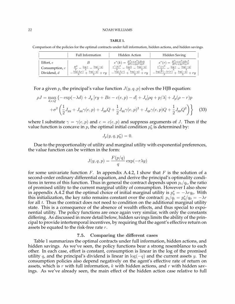
TABLE 1.

Comparison of the policies for the optimal contracts under full information, hidden actions, and hidden savings.

Full Information Hidden Action Hidden Saving

Effort, e B e∗(k) = B3r+σ2λBrkB2r+2σ2λk2 e∗(r) = B3r+σ2λBr2

B2r+2σ2λr2

Consumption, c B2

2− log r

λ− log(−q)

λe∗(k)2

2− log k

λ− log(−q)

λe∗(r)2

2− log r

λ− log(−q)

λ

Dividend, d − log(J0r)λ

+ log(−q)λ

+ ry − log(J1r)λ

+ log(−q)λ

+ ry − log(F (−λr)r)λ

+ log(−q)λ

+ ry

For a given p, the principal’s value function J(y, q, p) solves the HJB equation:

ρJ = maxd,e,Q

− exp(−λd) + Jy [ry + Be− c(e, p)− d] + Jq[ρq + p/λ] + Jp(ρ− r)p

+σ2

(1

2Jyy + Jyqγ(e, p) + JypQ +

1

2Jqqγ(e, p)2 + Jqpγ(e, p)Q +

1

2JppQ

2

)(33)

where I substitute γ = γ(e, p) and c = c(e, p) and suppress arguments of J . Then if thevalue function is concave in p, the optimal initial condition p∗0 is determined by:

Jp(y, q, p∗0) = 0.

Due to the proportionality of utility and marginal utility with exponential preferences,the value function can be written in the form:

J(y, q, p) =F (p/q)

qexp(−rλy)

for some univariate function F . In appendix A.4.2, I show that F is the solution of asecond-order ordinary differential equation, and derive the principal’s optimality condi-tions in terms of this function. Thus in general the contract depends upon pt/qt, the ratioof promised utility to the current marginal utility of consumption. However I also showin appendix A.4.2 that the optimal choice of initial marginal utility is p∗0 = −λrq0. Withthis initialization, the key ratio remains constant over the contract: pt/qt = p∗0/q0 = −λrfor all t. Thus the contract does not need to condition on the additional marginal utilitystate. This is a consequence of the absence of wealth effects, and thus special to expo-nential utility. The policy functions are once again very similar, with only the constantsdiffering. As discussed in more detail below, hidden savings limits the ability of the prin-cipal to provide intertemporal incentives, by requiring that the agent’s effective return onassets be equated to the risk-free rate r.

7.5. Comparing the different casesTable 1 summarizes the optimal contracts under full information, hidden actions, and

hidden savings. As we’ve seen, the policy functions bear a strong resemblance to eachother. In each case, effort is constant, consumption is linear in the log of the promisedutility q, and the principal’s dividend is linear in log(−q) and the current assets y. Theconsumption policies also depend negatively on the agent’s effective rate of return onassets, which is r with full information, k with hidden actions, and r with hidden sav-ings. As we’ve already seen, the main effect of the hidden action case relative to full


0 1 2 3

0.3

0.35

0.4

0.45

0.5

σ

efi,eha,ehs

Effort

FI

HA

HS

0 1 2 30.98

1

1.02

1.04

1.06

1.08Agent Consumption (q=−1)

σ

cfi,cha,chs

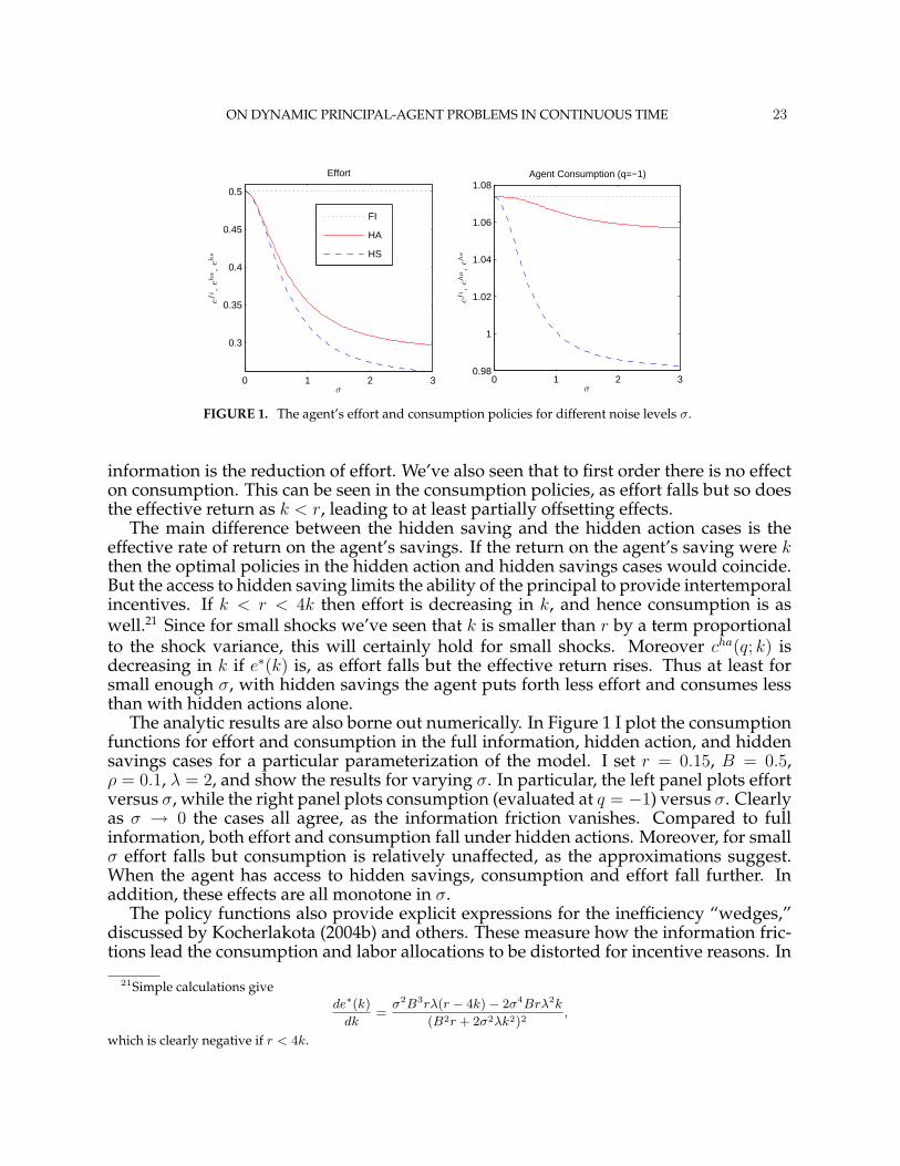
FIGURE 1. The agent’s effort and consumption policies for different noise levels σ.

information is the reduction of effort. We’ve also seen that to first order there is no effecton consumption. This can be seen in the consumption policies, as effort falls but so doesthe effective return as k < r, leading to at least partially offsetting effects.

The main difference between the hidden saving and the hidden action cases is theeffective rate of return on the agent’s savings. If the return on the agent’s saving were kthen the optimal policies in the hidden action and hidden savings cases would coincide.But the access to hidden saving limits the ability of the principal to provide intertemporalincentives. If k < r < 4k then effort is decreasing in k, and hence consumption is aswell.21 Since for small shocks we’ve seen that k is smaller than r by a term proportionalto the shock variance, this will certainly hold for small shocks. Moreover cha(q; k) isdecreasing in k if e∗(k) is, as effort falls but the effective return rises. Thus at least forsmall enough σ, with hidden savings the agent puts forth less effort and consumes lessthan with hidden actions alone.

The analytic results are also borne out numerically. In Figure 1 I plot the consumptionfunctions for effort and consumption in the full information, hidden action, and hiddensavings cases for a particular parameterization of the model. I set r = 0.15, B = 0.5,ρ = 0.1, λ = 2, and show the results for varying σ. In particular, the left panel plots effortversus σ, while the right panel plots consumption (evaluated at q = −1) versus σ. Clearlyas σ → 0 the cases all agree, as the information friction vanishes. Compared to fullinformation, both effort and consumption fall under hidden actions. Moreover, for smallσ effort falls but consumption is relatively unaffected, as the approximations suggest.When the agent has access to hidden savings, consumption and effort fall further. Inaddition, these effects are all monotone in σ.

The policy functions also provide explicit expressions for the inefficiency “wedges,”discussed by Kocherlakota (2004b) and others. These measure how the information fric-tions lead the consumption and labor allocations to be distorted for incentive reasons. In

21Simple calculations givede∗(k)

dk=

σ2B3rλ(r − 4k)− 2σ4Brλ2k

(B2r + 2σ2λk2)2,

which is clearly negative if r < 4k.

24 NOAH WILLIAMS

0 1 2 30

0.1

0.2

0.3

0.4

0.5

σ

τL

Labor Wedge

0 1 2 30

0.05

0.1

0.15Intertemporal Wedge

σ

τK

HA

HS

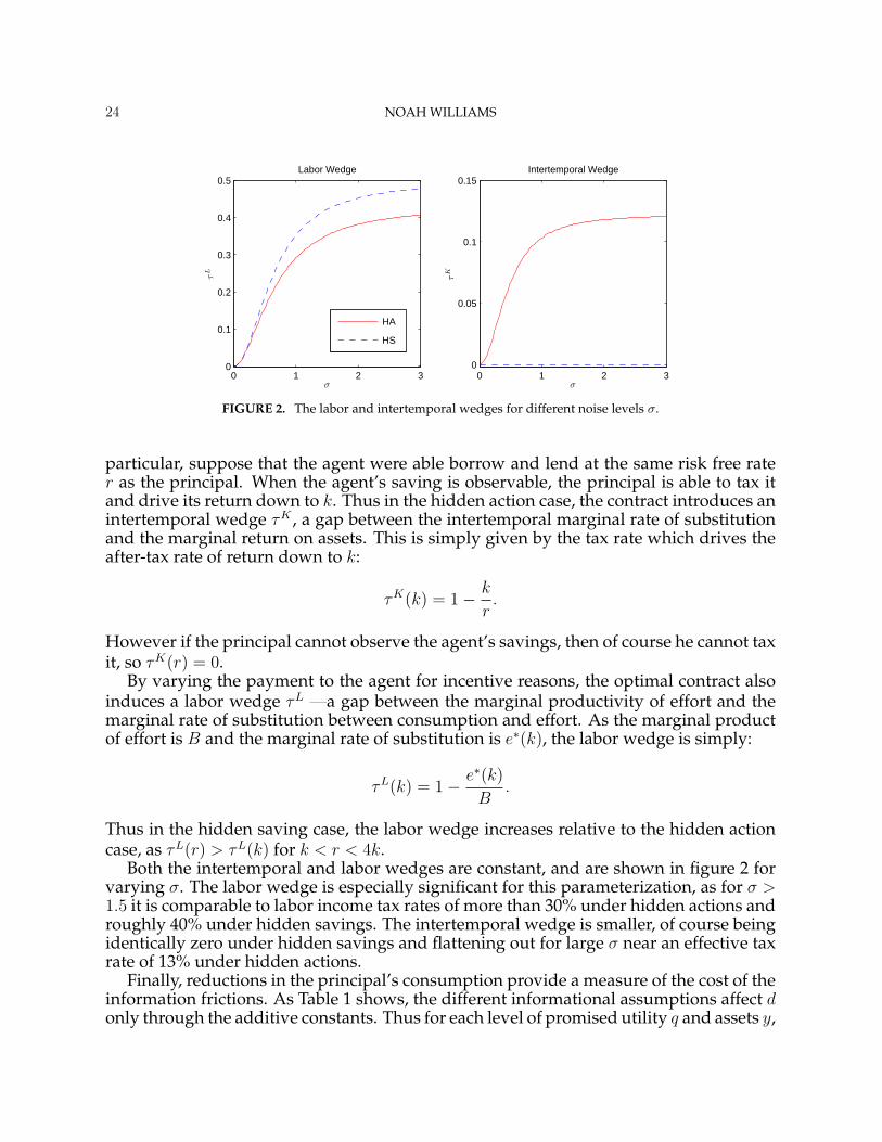
FIGURE 2. The labor and intertemporal wedges for different noise levels σ.

particular, suppose that the agent were able borrow and lend at the same risk free rater as the principal. When the agent’s saving is observable, the principal is able to tax itand drive its return down to k. Thus in the hidden action case, the contract introduces anintertemporal wedge τK , a gap between the intertemporal marginal rate of substitutionand the marginal return on assets. This is simply given by the tax rate which drives theafter-tax rate of return down to k:

τK(k) = 1− k

r.

However if the principal cannot observe the agent’s savings, then of course he cannot taxit, so τK(r) = 0.

By varying the payment to the agent for incentive reasons, the optimal contract alsoinduces a labor wedge τL —a gap between the marginal productivity of effort and themarginal rate of substitution between consumption and effort. As the marginal productof effort is B and the marginal rate of substitution is e∗(k), the labor wedge is simply:

τL(k) = 1− e∗(k)

B.

Thus in the hidden saving case, the labor wedge increases relative to the hidden actioncase, as τL(r) > τL(k) for k < r < 4k.

Both the intertemporal and labor wedges are constant, and are shown in figure 2 forvarying σ. The labor wedge is especially significant for this parameterization, as for σ >1.5 it is comparable to labor income tax rates of more than 30% under hidden actions androughly 40% under hidden savings. The intertemporal wedge is smaller, of course beingidentically zero under hidden savings and flattening out for large σ near an effective taxrate of 13% under hidden actions.

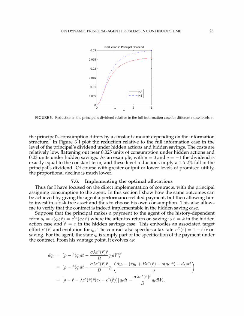
Finally, reductions in the principal’s consumption provide a measure of the cost of theinformation frictions. As Table 1 shows, the different informational assumptions affect donly through the additive constants. Thus for each level of promised utility q and assets y,


0 1 2 30

0.005

0.01

0.015

0.02

0.025

0.03Reduction in Principal Dividend

σ

HAHS

FIGURE 3. Reduction in the principal’s dividend relative to the full information case for different noise levels σ.

the principal’s consumption differs by a constant amount depending on the informationstructure. In Figure 3 I plot the reduction relative to the full information case in thelevel of the principal’s dividend under hidden actions and hidden savings. The costs arerelatively low, flattening out near 0.025 units of consumption under hidden actions and0.03 units under hidden savings. As an example, with y = 0 and q = −1 the dividend isexactly equal to the constant term, and these level reductions imply a 1.5-2% fall in theprincipal’s dividend. Of course with greater output or lower levels of promised utility,the proportional decline is much lower.

7.6. Implementing the optimal allocationsThus far I have focused on the direct implementation of contracts, with the principal

assigning consumption to the agent. In this section I show how the same outcomes canbe achieved by giving the agent a performance-related payment, but then allowing himto invest in a risk-free asset and thus to choose his own consumption. This also allowsme to verify that the contract is indeed implementable in the hidden saving case.

Suppose that the principal makes a payment to the agent of the history-dependentform st = s(qt; r) = cha(qt; r) where the after-tax return on saving is r = k in the hiddenaction case and r = r in the hidden savings case. This embodies an associated targeteffort e∗(r) and evolution for qt. The contract also specifies a tax rate τK(r) = 1 − r/r onsaving. For the agent, the state qt is simply part of the specification of the payment underthe contract. From his vantage point, it evolves as:

dqt = (ρ− r)qtdt− σλe∗(r)rB

qtdW e∗t

= (ρ− r)qtdt− σλe∗(r)rB

qt

(dyt − (ryt + Be∗(r)− s(qt; r)− dt)dt

σ

)

= [ρ− r − λe∗(r)r(et − e∗(r))] qtdt− σλe∗(r)rB

qtdWt.

26 NOAH WILLIAMS

Here I use the fact that W e∗t is the driving Brownian motion under the optimal contract

for the principal’s information set. Moreover the agent begins with zero wealth m0 = 0,which then evolves as:

dmt =([1− τK(r)]rmt + s(qt; r)− ct

)dt

=

(rmt +

e∗(r)2

2− log(r)

λ− log(−qt)

λ− ct

)dt

Thus the agent’s value function V (q,m) solves the HJB equation:

ρV (q,m) = maxc,e

− exp(−λ(c− e2/2)) + Vm(q, m) [rm + s(q; r)− c]

+Vq(q, m)q[ρ− r − λe∗(r)r(et − e∗(r))] +1

2Vqq(q,m)q2σ2λ2e∗(r)2r2

B2

It is easy to verify that the agent’s value function is given by V (q,m) = q exp(−λrm).Substituting this into the HJB equation, and taking first order conditions for (c, e) gives:

λ exp(−λ(c− e2/2)) = Vm = −λrq exp(−λrm),

λe exp(−λ(c− e2/2)) = −λe∗(r)rqVq = −λe∗(r)rq exp(−λrm).

Taking ratios of the two equations gives e = e∗, and thus the target effort level is imple-mentable. Since effort is independent of m, the sufficient condition (29) holds. Thus thecontract is indeed implementable.

It is also easy to directly verify implementability. The optimality condition for c gives:

c =e∗(r)2

2− log r

λ− log(−q)

λ+ rm.

Substituting this into the wealth equation gives dmt = 0. Thus, if the agent begins withmt = 0, then he will remain at zero wealth, will consume the optimal amount underthe contract c = cha(q; r), and will attain the value V (q, 0) = q. Therefore the policiesassociated with the optimal contracts can be implemented with this payment and savingstax scheme. In particular, the contract that we derived in the hidden saving case is indeedimplementable, even though the sufficient concavity conditions do not hold.

8. CONCLUSION

In this paper I have established several key results for dynamic principal-agent prob-lems. By working in a continuous time setting, I was able to take advantage of powerfulresults in stochastic control, which led to some sharp conclusions. I characterized theclass of implementable contracts in dynamic settings with hidden actions and hiddenstates via a first-order approach, providing a general proof of its validity in a dynamicenvironment. I showed that implementable contracts must respect some additional statevariables: the agent’s utility process and the agent’s “shadow value” (in marginal util-ity terms) of the hidden states. I then developed a constructive method for solving for


an optimal contract. The optimal contract is in general history dependent, but can bewritten recursively in terms of a small number of state variables.

As an application, I showed that as in Holmstrom and Milgrom (1987) the optimalcontract is linear in a fully dynamic setting with exponential utility. However now thepayment is linear in an endogenous object, the logarithm of the agent’s promised utilityunder the contract. Moreover, I showed that the main effect of hidden actions is to re-duce effort, with a smaller effect on the agent’s implicit rate of return under the contract,which in turn affects consumption. Introducing hidden savings eliminates this seconddistortion, and increases the effort distortion.

Overall, the methods developed in the paper are tractable and reasonably general,making a class of models amenable to analysis. In Williams (2008) I apply the results inthis paper to study borrowing and lending contracts when agents have persistent privateinformation. Given the active literature on dynamic models with information frictionswhich has developed in the past few years, there is broad potential scope for furtherapplications of my results.

APPENDIX

A.1. DETAILS OF THE CHANGE OF MEASURE

Here I provide technical detail associated with the change of measure in Section 3.2. I start by working with theinduced distributions on the space of continuous functions, which I take to be the underlying probability space. Thus Ilet the sample space Ω be the space Cny , and let W 0

t = ω(t) be the family of coordinate functions, and F0t = σW 0

s s ≤t the filtration generated by W 0

t . I let P be the Wiener measure on (Ω,F0T ), and let Ft be the completion of F0

t withthe null sets of F0

T . This defines the basic (canonical) filtered probability space, on which is defined the Brownianmotion W 0

t . I now introduce some regularity conditions on the diffusion coefficient in (11) following Elliott (1982).

Assumptions A.1. Denote by σij(t, y, s) the (i, j) element of the matrix σ(t, y, s). Then I that for all i, j, for somefixed K independent of t and i, j:

1. σij is continuous,

2. |σij(t, y, s)− σij(t, y′, s′)| ≤ K (|y − y′|+ |s− s′|),

3. σ(t, y, s) is non-singular for each (t, y, s) and |(σ−1(t, y, s))ij | ≤ K.

Of these, the most restrictive is perhaps the nonsingularity condition, which requires that noise enter every partof the state y. Under these conditions, there exists a unique strong solution to the stochastic differential equation:

dyt = σ(t, y, Z)dW 0t , (A.1)

with y0 given. This is the evolution of output under an effort policy e0 which makes f(t, y, mt, e0t ) = 0 at each date.

Different effort choices alter the evolution of output by changing the distribution over outcomes in Cny .Now I state some required regularity conditions on the drift function f .

Assumptions A.2. I assume that for some fixed K independent of t:

1. f is continuous,

2. |f(t, y, m, e, s)| ≤ K(1 + |m|+ |y|+ |s|).

These imply the predictability, continuity, and linear growth conditions on the concentrated function f which areassumed by Elliott (1982). Then for e ∈ A I define the family of Ft-predictable processes:

Γt(e) = exp

(∫ t

0

σ−1(v, y)f(v, y, mv, ev)dW 0v − 1

2

∫ t

0

|σ−1(v, y)f(v, y, mv, ev)|2dv

).

28 NOAH WILLIAMS

Under the conditions above, Γt is an Ft-martingale (as the assumptions insure that Novikov’s condition is satisfied)with E[ΓT (e)] = 1 for all e ∈ A. Thus by the Girsanov theorem, I can define a new measure Pe via:

dPe

dP= ΓT (e),

and the process W et defined by:

W et = W 0

t −∫ t

0

σ−1(v, y)f(v, y, mv, ev)dv

is a Brownian motion under Pe. Thus from (A.1), it’s clear that the state follows the SDE:

dyt = f(t, y, mt, et)dt + σ(t, y)dW et .

Hence each effort choice e results in a different Brownian motion. Γt defined above (suppressing e) satisfies Γt =

E[ΓT |Ft], and thus is the relative density process for the change of measure.

A.2. ASSUMPTIONS FOR RESULTS

Here I list some additional regularity conditions. The first is a differentiability assumption for the agent’s problem.

Assumption A.3. The functions (u, v, f, b) are continuously differentiable in m.

The next sets of assumptions guarantee that the local incentive constraint is satisfied in the hidden action andhidden state cases.

Assumptions A.4. The function u is concave in e, f is concave in e, and and uefe ≤ 0.

Assumptions A.5. The function u is separable in e and c and concave in (e, c), b is concave in c, and ucbc ≤ 0.

A.3. PROOFS OF RESULTS

Proof (Proposition 4.1). This follows by applying the results in Bismut (1973)-(1978) to my problem. Under theassumptions, the maximum principle applies to the system with (Γ, x) as the state variables. I now illustrate thecalculations leading to the Hamiltonian (16) and the adjoint equations (17)-(18). I first define the stacked system:

Xt =

[Γt

xt

], Θt =

[qt

pt

], Λt =

[γt

Qt

].

Then note from (14)-(15) that Xt satisfies (suppressing arguments):

dXt = Γt

[0

b

]dt + Γt

[σ−1f

mtσ−1f

]dW 0

t

= M(t)dt + Σ(t)dW 0t

Thus, as in Bismut (1978), the Hamiltonian for the problem is:

H = ΘM + tr(Λ′Σ) + Γu = ΓH,

where H is from (16). As Γ ≥ 0, the optimality condition (19) is the same with H or H . The adjoint variables follow:

dΘt = −∂H

∂X(t)dt + ΛtdW 0

t

ΘT =∂(ΓT v(yT , mT ))

∂XT.

By carrying out the differentiation and simplifying I arrive at (17)-(18).


Proof (Proposition 5.1). The result is an extension of Theorem 4.2 in Schattler and Sung (1993). The necessity ofthe conditions follow directly from my results above: if the contract is implementable then it clearly must satisfy theparticipation constraint, and by Proposition 4.1 it must satisfy promise-keeping and be locally incentive compatible.

To show the converse, I verify that e is an optimal control when the agent faces the contract (s, e). Recall that theexpected utility from following e is given by V (e) = q0. From the results above, for any e ∈ A the following holds:

V (e)− V (e) = Ee

[∫ T

0

[u(t, yt, et, st)− u(t, yt, et, st)]dt +

∫ T

0

γtσ(t, yt, st)dW et

]

= Ee

[∫ T

0

[u(t, yt, et, st)− u(t, yt, et, st)]dt +

∫ T

0


]

+Ee

[∫ T

0

γt [f(t, yt, et, st)− f(t, yt, et, st)]dt

]

= Ee

[∫ T

0

[H∗(t, et)−H∗(t, et)]dt +

∫ T

0


]

≤ Ee

[∫ T

0


]= 0.

Here the first equality uses (22), the second equality uses the definitions of the change of measure between W e andW e, the third equality uses the definition of the H∗ function in (23), the inequality follows from the local incentiveconstraint (24), and the final result uses the fact that the stochastic integral is a martingale due to the square inte-grability of the γtσ(t) process. Thus since e was arbitrary, the agent can achieve at most the utility V (e) which isgreater than his reservation level by assumption. Thus e is an optimal control, and so the contract is implementable.

Proof (Proposition 5.2). This proof combines ideas from Schattler and Sung (1993) with those in Zhou (1996). Thenecessity of the conditions follows directly as in Proposition 5.1 above, as it is a consequence of Proposition 4.1.

To show the converse, I consider an arbitrary (e, c) which imply a process m = mt. Under my assumptions thelocal incentive constraint (28) ensures that:

H∗∗e (t, mt, et, ct) = H∗∗

c (t, mt, et, ct) = 0.

Thus by the concavity of H∗∗, for any (mt, et, ct) we get:

H∗∗(t, mt, et, ct)−H∗∗(t, mt, et, ct) ≤ 〈H∗∗m (t, mt, et, ct), mt − mt〉. (A.2)

I extend the shorthand notation above to now write b(t) = b(t, mt, ct, st) and so on. Then I define ∆t = mt − mt,and I can write its evolution as:

d∆t = [bm(t)∆t + αt]dt, (A.3)

with ∆0 = 0 where I define:

αt = −bm(t)∆t + b(t)− b(t)

Then we have the following relationship between pt in (18) for the target policy and ∆t in (A.3):

vm(T )∆t = pT ∆T =

∫ T

0

[∆tdpt + ptd∆t]

=

∫ T

0

(αtpt −∆t

[(γt + Qtmt)fm(t) + Qtf(t) + um(t)

])dt +

∫ T

0

∆tQtσ(t)dW 0t

Hence by the concavity of v I have:

Ee[v(T )− v(T )] ≤ Ee[vm(T )∆T ] = Ee

[∫ T

0

(ptαt −

[(γt + Qtmt)fm(t) + um(t) + Qt(f(t)− f(t))

]∆t

)dt

], (A.4)

where the final term in Qt is due to the change from the base measure P0 to Pe (associated with e).

30 NOAH WILLIAMS

Then I proceed as in Proposition 5.1 and note that for any (e, c) ∈ A I have:

V (e, c)− V (e, c) = Ee

[∫ T

0

[u(t)− u(t)]dt +

∫ T

0

[γt + Qtmt]σ(t)dW et + v(T )− v(T )

]

= Ee

[∫ T

0

[u(t)− u(t) + (γt + Qtmt)(f(t)− f(t))]dt +

∫ T

0

[γt + Qtmt]σ(t)dW et + v(T )− v(T )

]

≤ Ee

[∫ T

0

(u(t)− u(t) + [γt + Qtmt]f(t) + ptαt −

[(γt + Qtmt)fm(t) + um(t) + Qt(f(t)− f(t))

]∆t

)dt

]

= Ee

[∫ T

0

(u(t)− u(t)− um(t)∆t + (γt + Qtmt)(f(t)− f(t))− (γt + Qtmt)∆tfm(t)

)dt

]

+Ee

[∫ T

0

(pt[b(t)− b(t)− bm(t)∆t]

)dt

](A.5)

= Ee

[∫ T

0

[H∗∗(t)−H∗∗(t)−H∗∗m (t)∆t]dt

]≤ 0.

Here the first equality uses (27), while the second equality uses the definitions of the change of measure between Pe

and Pe. The following inequality uses (A.4), while the next equality uses the definition of αt. The following equalityuses the definition of H∗∗ in (26), and the final result follows from its concavity as in (A.2). Thus since (e, c) wasarbitrary, we see that (e, c) is an optimal control, and the contract is thus implementable.

The weaker sufficient condition (29) stated in section 5.3 uses (A.5) along with the fact that the local incentive con-straint implies that H∗∗(t, m, et, ct) ≥ H∗∗(t, m, et, ct).

Proof (Corollary 5.1 and 5.2). In either case, the stated assumptions insure that H∗ is concave in e and H∗∗

is concave in (e, c). This is clear from (21) in the hidden action case. The parallel first order conditions give theresult in the hidden state case, where the separability insures that I can simply look at the separate first order con-ditions. But by assumption, each function has a stationary point on the feasible set, which is then a maximum.

A.4. DETAILED CALCULATIONS FOR THE EXAMPLE

A.4.1. The hidden action caseHere we provide explicit expressions for the key constants which determine the policy functions in the hidden

action case. Note that u(t, c(q), e∗) = e−ρtkq. Using this along with the form of the value function in the first orderconditions for (e, c) determines the equations that e∗ and k must satisfy:

r − k + σ2rλ2e∗k/B − 2σ2λ2(e∗)2k2/B2 = 0, (A.6)

−Br + λe∗k − σ2rλ(1 + λ(e∗)2)k/B − 2σ2λe∗(1 + λ(e∗)2)k2/B2 = 0.

These can be solved to get e∗(k):

e∗ =B3r + σ2λBrk

B2r + 2σ2λk2, (A.7)

then substituting this back into the first equation in (A.6) gives an expression for k. Notice that for σ = 0 thesecollapse to the full information solution e∗ = B and k = r. The constant J1 is determined from the HJB equation aftersubstituting in the optimal policies, which implies:

J1 =1

krexp

(r + k − 2ρ

rA− λe∗

(B − e∗

2

)+ σ2λ2

(r

2− e∗k

B+

(e∗)2k2

rB2

)).

A.4.2. The hidden saving caseI now derive the optimality conditions in the hidden savings case. To simplify notation, I define z = p/q as the

argument of the F function, noting that z ∈ (−∞, 0). Thus the optimality condition for p∗0 translates to F ′(z∗0) = 0, orp∗0 = (F ′)−1(0)q0. Using the guess of the form of the solution in the HJB equation (33), I take the first order condition


for the dividend, and obtain a policy function similar to the hidden action case:

dhs(y, q, z) = − log(F (z)r)

λ+

log(−q)

λ+ ry.

For the volatility of marginal utility, I find it convenient to normalize Qt = Qtpt. Then the optimal choices of e and Q

are determined by the first order conditions:

−λrF (z)(B − e) +(F ′′(z)z2 + 4F ′(z)z + 2F (z)

) σ2z2e

B2

+λr(F ′(z)z + F (z))σ2z

B− (2F ′(z) + F ′′(z)z)Q

σ2z2

B= 0, (A.8)

F ′′(z)zQ− λrF ′(z)− (2F ′(z) + F ′′(z)z)ez

B= 0. (A.9)

Thus given F , these equations determine the optimal policies as a function of z alone: ehs(z) and Q(z). Substitutingthese into (33), I find that F is the solution of the second order ODE:

ρF (z) = rF (z)− (F ′(z)z + F (z))(ρ + z/λ)− λrF (z)

[Behs(z)− ehs(z)2

2+

log(−rzF (z)/λ)

λ

]

+(ρ− r)zF ′(z) + (F ′′(z)z2 + 4F ′(z)z + 2F (z))σ2ehs(z)2z2

2B2+ (F ′(z)z + F (z))

σ2λrehs(z)z

B

+σ2

(λ2r2

2F (z) + F ′′(z)z2 Q(z)2

2− λrF ′(z)zQ(z)− (2F ′(z) + F ′′(z)z2)

ehs(z)Q(z)z2

B

),

with the boundary conditions limz→0 F (z) = ∞ and limz→−∞ F (z) = ∞. These conditions imply that the principal’sutility falls without bound as the agent’s current consumption or future promised utility increase without bound.

Thus I have reduced the solution of the three dimensional PDE for the value function to an ODE. The ODE issufficiently complex that an explicit solution for arbitrary z does not seem feasible. However, I can obtain moreexplicit results for the value and the policies at the optimal starting value z∗0 . At z∗0 (A.8) and (A.9) imply:

Q(z∗0) =ehs(z∗0)z∗0

B, e∗0 = ehs(z∗0) =

B3r − σ2Brz∗0B2r + 2σ2(z∗0)2/λ

.

Then using these in the ODE we get:

F (z∗0) =−λ

rz∗0exp

(λr − z∗0 − 2λρ

λr− λe∗0

(B − e∗0

2

)+ σ2λ2

(r

2+

e∗0z∗0

λB+

(e∗0z∗0)2

λrB2

)).

Note that if z∗0 = −λk then these results agree with the hidden action case, as ehs(−λk) = e∗ from (A.7) andF (−λk) = J1. But this is indeed the optimal choice of z0 when the return on the agent’s saving differs from theprincipal’s and is equal to k. This can be verified analytically by implicitly differentiating the ODE for F and usingthe expressions for ehs(z∗0) and Q(z∗0) to solve for z∗0 . However in general I cannot analytically solve for the optimalstarting value, and so I numerically solve the ODE for F (z), then choose z∗0 as the minimizing value. (These calcula-tions are straightforward but lengthy and thus are not included here. Details can be furnished upon request.) For theparametrization below, I find that z∗0 = −λr. I have also verified the same result in alternative parameterizations.

These results imply that zt is in fact constant over time, which follows from the evolution of zt:

dzt = −[(zt/λ + r)zt +

σ2ehs(zt)2z2

t

B

(Q(zt)− ehs(zt)zt

B

)]dt + σzt

(Q(zt)− ehs(zt)zt

B

)dWt.

Using the expression for Q(z∗0) above, note that dzt = 0 if z∗0 = −λr. Therefore utility and marginal utility remainproportional forever under the contract.

References

Abraham, A. and N. Pavoni (2008). Efficient Allocations with Moral Hazard and Hid-den Borrowing and Lending. Review of Economic Dynamics, forthcoming.

32 NOAH WILLIAMS

Abreu, D., D. Pearce, and E. Stacchetti (1986). Optimal Cartel Equilibria with ImperfectMonitoring. Journal of Economic Theory 39, 251–269.

Abreu, D., D. Pearce, and E. Stacchetti (1990). Toward a Theory of Discounted RepeatedGames with Imperfect Monitoring. Econometrica 58, 1041–1063.

Allen, F. (1985). Repeated Principal-Agent Relationships with Borrowing and Lending.Economics Letters 17, 27–31.

Bismut, J. M. (1973). Conjugate Convex Functions in Optimal Stochastic Control. Jour-nal of Mathematical Analysis and Applications 44, 384–404.

Bismut, J. M. (1975). Growth and the Optimal Intertemporal Allocation of Risks. Journalof Economic Theory 10, 239–257.

Bismut, J. M. (1978). Duality Methods in the Control of Densities. SIAM Journal onControl and Optimization 16, 771–777.

Bolton, P. and M. Dewatripont (2005). Contract Theory. Cambridge: MIT Press.Brock, W. A. and M. J. Magill (1979). Dynamics Under Uncertainty. Econometrica 47,

843–868.Cadenillas, A., J. Cvitanic, and F. Zapatero (2005). Dynamic Principal-Agent Problems

with Perfect Information. Working paper, USC.Chari, V. V., P. J. Kehoe, and E. McGrattan (2007). Business Cycle Accounting. Econo-

metrica 75, 781–836.Cole, H. L. and N. Kocherlakota (2001). Efficient Allocations with Hidden Income and

Hidden Storage. Review of Economic Studies 68, 523–542.Cox, J., S. Ross, and M. Rubinstein (1979). Option Pricing: A Simplified Approach.

Journal of Financial Economics 7, 229–263.Cvitanic, J., X. Wan, and J. Zhang (2006). Continuous-Time Principal-Agent Problems

with Hidden Action and Lump-Sum Payment. Working paper, USC.Detemple, J., S. Govindaraj, and M. Loewenstein (2005). Wealth-Robust Intertemporal

Incentive Contracts. Working paper, Boston University.Doepke, M. and R. M. Townsend (2006). Dynamic Mechanism Design with Hidden

Income and Hidden Storage. Journal of Economic Theory 126, 235–285.El Karoui, N., S. Peng, and M. C. Quenez (1997). Backward Stochastic Differential

Equations in Finance. Mathematical Finance 7, 1–71.Elliott, R. J. (1982). Stochastic Calculus and Applications. New York: Springer-Verlag.Fudenberg, D., B. Holmstrom, and P. Milgrom (1990). Short-Term Contracts and Long-

Term Agency Relationships. Journal of Economic Theory 51, 1–31.Golosov, M., N. Kocherlakota, and A. Tsyvinski (2003). Optimal Indirect and Capital

Taxation. Review of Economic Studies 70, 569–587.Hellwig, M. F. and K. M. Schmidt (2002). Discrete-Time Approximations of the

Holmstrom-Milgrom Brownian-Motion Model of Intertemporal Incentive Provi-sion. Econometrica 70, 2225–2264.


Holmstrom, B. and P. Milgrom (1987). Aggregation and Linearity in the Provision ofIntertemporal Incentives. Econometrica 55, 303–328.

Hopenhayn, H. A. and J. P. Nicolini (1997). Optimal Unemployment Insurance. Journalof Political Economy 105, 412–38.

Jewitt, I. (1988). Justifying the First-Order Approach to Principal-Agent Problems.Econometrica 56, 1177–1190.

Karatzas, I. and S. E. Shreve (1991). Brownian Motion and Stochastic Calculus (2nd ed.).New York: Springer-Verlag.

Kocherlakota, N. R. (2004a). Figuring Out The Impact of Hidden Savings on OptimalUnemployment Insurance. Review of Economic Dynamics 7, 541–554.

Kocherlakota, N. R. (2004b). Wedges and taxes. American Economic Review (Papers andProceedings) 94, 109–113.

Ma, J. and J. Yong (1999). Forward-Backward Stochastic Differential Equations and Their Ap-plications, Volume 1702 of Lecture Notes in Mathematics. New York: Springer-Verlag.

Mirrlees, J. A. (1999). The Theory of Moral Hazard and Unobservable Behaviour: PartI. Review of Economic Studies 66, 3–21.

Phelan, C. and E. Stacchetti (2001). Sequential Equilibria in a Ramsey Tax Model. Econo-metrica 69, 1491–1518.

Rogerson, W. P. (1985a). Repeated Moral Hazard. Econometrica 53, 69–76.Rogerson, W. P. (1985b). The First-Order Approach to Principal-Agent Problems.

Econometrica 53, 1357–1367.Sannikov, Y. (2008). A Continuous-Time Version of the Principal-Agent Problem. Re-

view of Economic Studies 75, 957–984.Schattler, H. and J. Sung (1993). The First-Order Approach to the Continuous-Time

Principal-Agent Problem with Exponential Utility. Journal of Economic Theory 61,331–371.

Spear, S. and S. Srivastrava (1987). On Repeated Moral Hazard with Discounting. Re-view of Economic Studies 53, 599–617.

Sung, J. (1997). Corporate Insurance and Managerial Incentives. Journal of EconomicTheory 74, 297–332.

Werning, I. (2002). Optimal Unemployment Insurance with Unobservable Saving.Working paper, MIT.

Westerfield, M. (2006). Optimal Dynamic Contracts with Hidden Actions in Continu-ous Time. Working paper, USC.

Williams, N. (2008). Persistent Private Information. Working paper, University of Wis-consin.

Yong, J. and X. Y. Zhou (1999). Stochastic Controls. New York: Springer-Verlag.Zhou, X. Y. (1996). Sufficient Conditions of Optimality for Stochastic Systems with

Controllable Diffusions. IEEE Transactions on Automatic Control AC-41, 1176–1179.

Documents

On Dynamic Principal-Agent Problems in Continuous …nwilliam/dynamic-pa1.pdf · On Dynamic Principal-Agent Problems in ... contract by solving a partial differential equation