Embed Size (px)
Citation preview

9th
European Workshop on Structural Health Monitoring
July 10-13, 2018, Manchester, United Kingdom
Creative Commons CC-BY-NC licence https://creativecommons.org/licenses/by-nc/4.0/
Multi-agent fusion system based on sparse dynamic classifier selection
for bolt loosening monitoring
Dong Liang
Coll Internet Things, Hohai University, Nanjing 210098, Jiangsu, China,
E-mail: [email protected]
Abstract
In this project, for the problem of reliable damage assessment in large-scale aeronautical
structural health monitoring system, combining compressive sampling with multi-agent
method, we study that the sparse representation of damage information, aiming at
improving the system's data processing capabilities, collaboration capabilities and
dynamic adaptability for the reliably and effectively damage assessment in real time by
effectively coordinating and managing assessment methods in large aeronautical
structures. Hence, a multi-agent decision fusion method based on sparse dynamic
classifiers selection for large-scale aeronautical structures is proposed to reduce the
environment uncertainties on multi-sensor damage features and to improve the
identification efficiency of damage classification systems. According to the sparse
representation theory of compressed sampling, the relationship between damaged
sample features and the environment dynamic changes is studied through the sparse
representation of the training samples set and the testing samples. With the obtained
corresponding relationship between each sparse atom and each classifier group set, the
optimal classifier combination is selected in real-time from the idle classifier agents. It
can dynamically limit the number of classifier agents of contract net bidding and
improve the system's dynamic adaptability. It can also ensure the fusion accuracy of
multi-damage classification system and the real-time performance relative to static
classifier selection. The above research is of great practical significance to promote the
real practicality of structural health monitoring technology in the engineering field.
1. Introduction
Bolted joint is widely used in mechanical and architectural structures, such as machine
tools, industrial robots, transport machines, power plants, aviation stiffened plate,
bridges, and steel towers and so on. The bolt loosening induced by flight load and
environment factor can cause joint failure leading to a disastrous accident for the
aircraft. In order to keep up the integrity and operation safety of these structures,
detecting bolted joint in real-time is an important concern in structural health
monitoring.
Till now, for the bolt loosening detection, there are some conventional non-destructive
inspection techniques, which use the ultrasonic waves and electromagnetic resonance
[1,2]. However, these methods are costly, labor intensive and time consuming to
perform for a large structure, and can only be performed when the aircraft is out of
service, being intermittent condition monitoring. Accordingly, structural health
monitoring (SHM) has being recently focused on by many researchers since the new
Mor
e in
fo a
bout
this
art
icle
: ht
tp://
ww
w.n
dt.n
et/?
id=
2332
7
2
inspection approach utilizes advanced sensor and actuator devices being integrated in
the structural material with aim to achieve a wide range of real-time online monitoring.
There are a number of significant works in the SHM area concerning bolt loosening
monitoring [3-12].
Recently, the development of artificial intelligence techniques has led to their
application in the structure health monitoring. Some methods, such as artificial neural
networks, support vector machines, and so on, have been employed to estimate the
structure damage [13, 14]. It is capable of modeling extremely complex nonlinear
relationships between known structure damage and structure output response. However,
for environment uncertainties, a decision fusion method can only acquire a limited
recognition capability for special data. Therefore, a multi-agent decision fusion method
based on sparse dynamic classifiers selection is introduced to combine compressive
sampling with multi-agent method, aiming at improving the system's data processing
capabilities, collaboration capabilities and dynamic adaptability for the reliably and
effectively damage assessment in real time.
The paper proposes a multi-agent decision fusion method based on sparse dynamic
classifiers selection for large-scale aeronautical structures. The rest of this paper is
structured in the following manner. Section 2 introduces the background knowledge of
compressed sampling, sparse dynamic classifier selection, and decision fusion. Section
3 gives experimental results and discussion for large aviation aluminum plate structure.
Finally, Section 4 concludes the paper.
2. Theory This section covers a brief introduction of decision fusion method, which consists of the
compressive sampling theory, sparse dynamic classifier selection and multi-agent fusion
method.
2.1 Compressive Sampling
The core idea of compressive sampling theory: if the original signal is sparse or it can
be expressed as sparse in some transform domain, so the original signal can be observed
through measurement matrix at the rate which is far lower than the required rate of the
Nyquist sampling theorem. And signal value whose number is more was projected to
the low-dimensional matrix to get the measured value whose number is far less than the
one of original data. Then the appropriate reconstruction algorithm was taken for those
measured value to accurately reconstruct and finally get the original signal. The essence
of compressive sampling is to sample directly compressed data.
The process of compressive sampling theory’s application mainly includes three parts as
follows[15].
2.1.1 Sparse representation of signal
Supposing that the original signal ( )x t is a column vector composed of one dimensional
discrete signal, then the original signal can be represented as follows:
=Ψx α (1)
whereα is a vector of weight coefficient and Ψ is the basis matrix. Ifα only
owns K non-zero (or the absolute value is larger) coefficients, while other N K−
coefficients are zero (or the absolute value is very small). So x is called K-sparse.
3
WhenK N<< , x is called that it possesses the character of sparsity and can be
compressed.
2.1.2 Measurement matrix
Supposing that the length of K-sparse discrete signal x is N , then that needs to
construct a M N× order matrix Φ as measurement matrix (K M N< < ). So the inner
product value y of measurement matrix Φ and discrete signal x is the measurement
value. And according to the equation (1), y can be written as follows:
= = =Φ ΦΨ Θy x α α (2)
Thus the sampling number of signal is M (the length of y )that is far less than the
length N of the original signal x .
2.1.3 Signal reconstruction algorithm
The process of the signal reconstruction is the process of solving an underdetermined
system of equations. Therefore, according to the principle of the equation (2), y was
used to solve x . In addition, the length of y is M and the length of x is N (M N≤ ).
The solving essence of the underdetermined equation is the solving problem of the
minimum 0l norm.
1argmin . . =Φx s t y x (3)
In fact, it is a problem of NP-Hard (Non-Convex Optimization Program). Therefore, the
process of signal reconstruction is turned into an optimization problem of the minimum
1l norm.
2.2 Sparse dynamic classifier selection
For the multi-sensor damage feature samples with the signal processing, the relationship
between the damage features and the dynamic uncertainties of the outside world is
studied through the selection of the training classifier set, the sparsification of the
training damage feature sample set, and the sparse representation of the test damage
features. The space-time correlation between the features of the test will be used to
sparsely extract the classifiers of the training samples corresponding to the sparse items
on the overcomplete dictionary set formed by the training samples so as to reduce the
influence of uncertainties and achieve the selection of sparse dynamic classifiers. The
processes are as follows:
Firstly, from a multi-sensor acquisition of health signals and feature samples with
complete failure and partial failure of each fastener, a certain number of training feature
sample sets are collected.
Then, base classifier selection is performed according to the classifier's own
characteristics and diversity. The classifier group is selected. For instance, SVM
classifier, BP neural network classifier, k-nearest neighbor classifier, Gaussian mixture
model GMM classifier, and improved iterative proportional IIS classifier are mainly
used. On the base, a representative base classifier group is selected by Bagging method
to get the initial classifier group system { 1,2,..., }i
E C i n= = , wehre n is the number of
classifiers, that is, the classifier body group system.
4
Moreover, according to the damage pattern class, some samples from each type of
training sample is selected as the initial dictionary , 1,2,...,iD i n= , n is the sample class
number. The K-SVD method is used for sparse representation and dictionary updating
to obtain all synthetic dictionaries 1 2
[ , ,..., ]n
D D D D= . Next, the sample set with k
neighbors of each atom in the training set is used to test the initial classifier set system
and the selection is achieved. The classifier with a rate of 0.5 is used as the classifier
corresponding , 1,2,...,iE E i m⊂ = of the atom, and m is the number of atoms. The
above two steps are used to reduce the influence of factors on the mean squared error of
the damage feature.
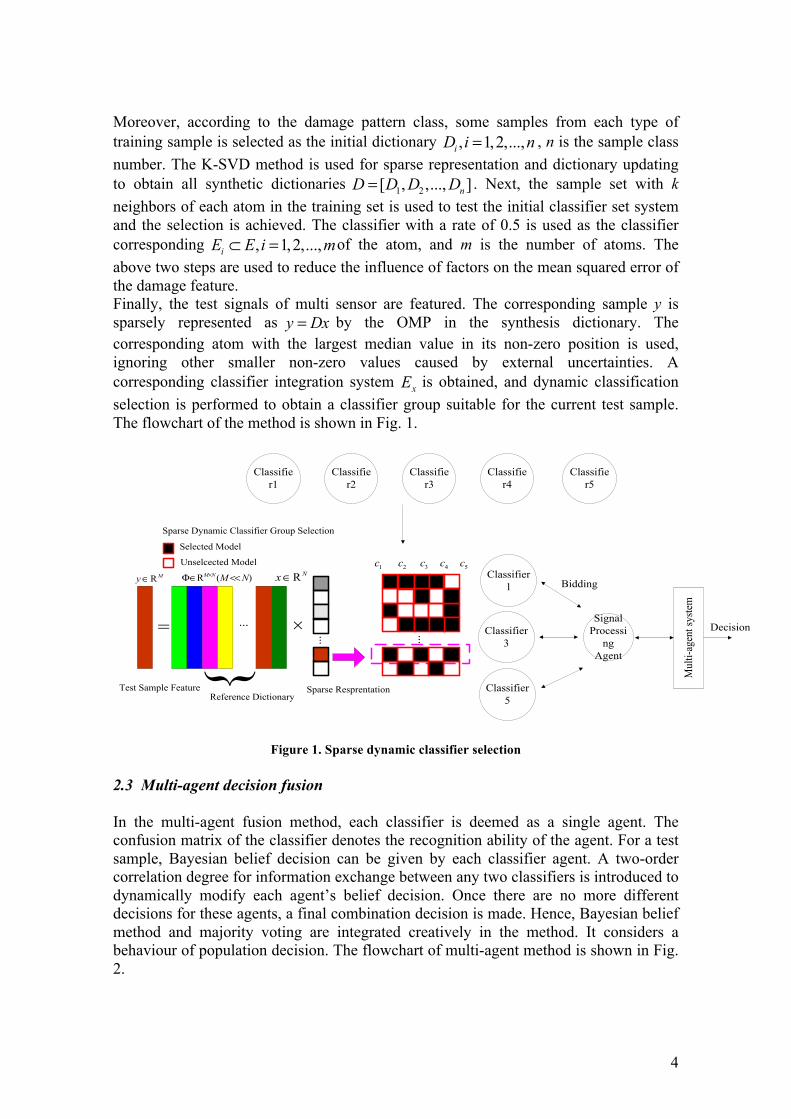
Finally, the test signals of multi sensor are featured. The corresponding sample y is
sparsely represented as y Dx= by the OMP in the synthesis dictionary. The
corresponding atom with the largest median value in its non-zero position is used,
ignoring other smaller non-zero values caused by external uncertainties. A
corresponding classifier integration system xE
is obtained, and dynamic classification
selection is performed to obtain a classifier group suitable for the current test sample.
The flowchart of the method is shown in Fig. 1.
Decision
Classifie
r1
Mult
i-ag
ent
syst
em
Classifie
r2
Classifie
r3
Classifie
r4
Classifie
r5
Classifier
3
Classifier
1
Classifier
5
Signal
Processi
ng
Agent
Bidding
Sparse Dynamic Classifier Group Selection
Selected Model
Unselcected Model1c 2c 3c 4c 5c
= ... × ...
...
Test Sample FeatureReference Dictionary
Sparse Resprentation{
R ( )M NM N
×Φ∈ << RN
x∈RMy∈
Figure 1. Sparse dynamic classifier selection
2.3 Multi-agent decision fusion
In the multi-agent fusion method, each classifier is deemed as a single agent. The
confusion matrix of the classifier denotes the recognition ability of the agent. For a test
sample, Bayesian belief decision can be given by each classifier agent. A two-order
correlation degree for information exchange between any two classifiers is introduced to
dynamically modify each agent’s belief decision. Once there are no more different
decisions for these agents, a final combination decision is made. Hence, Bayesian belief
method and majority voting are integrated creatively in the method. It considers a
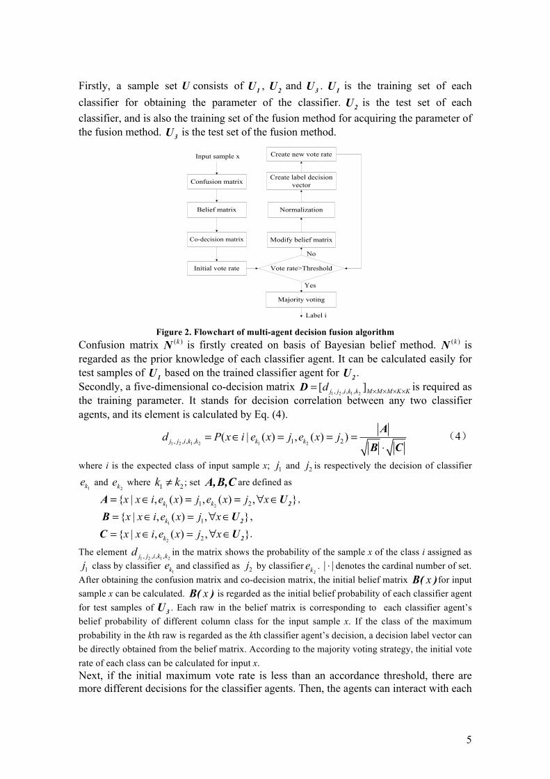
behaviour of population decision. The flowchart of multi-agent method is shown in Fig.
2.
5
Firstly, a sample set U consists of 1U ,
2U and
3U .
1U is the training set of each
classifier for obtaining the parameter of the classifier. 2
U is the test set of each
classifier, and is also the training set of the fusion method for acquiring the parameter of
the fusion method. 3
U is the test set of the fusion method.
Confusion matrix
Majority voting
Belief matrix
Co-decision matrix
Initial vote rate Vote rate>Threshold
Create new vote rate
Create label decision
vector
Normalization
Modify belief matrix
Input sample x
No
Label i
Yes
Figure 2. Flowchart of multi-agent decision fusion algorithm
Confusion matrix ( )kN is firstly created on basis of Bayesian belief method. ( )k
N is
regarded as the prior knowledge of each classifier agent. It can be calculated easily for
test samples of 1U based on the trained classifier agent for
2U .
Secondly, a five-dimensional co-decision matrix 1 2 1 2, , , ,
[ ]j j i k k M M M K Kd× × × ×
=D is required as
the training parameter. It stands for decision correlation between any two classifier
agents, and its element is calculated by Eq. (4).
1 2 1 2 1 2, , , , 1 2( | ( ) , ( ) )j j i k k k kd P x i e x j e x j= ∈ = = =
⋅
A
B C
4
where i is the expected class of input sample x; 1j and
2j is respectively the decision of classifier
1ke and
2ke where
1 2k k≠ ; set A,B,C are defined as
1 21 2{ | , ( ) , ( ) , }k kx x i e x j e x j x= ∈ = = ∀ ∈2
A U ,
1 1{ | , ( ) , }kx x i e x j x= ∈ = ∀ ∈2
B U ,
2 2{ | , ( ) , }kx x i e x j x= ∈ = ∀ ∈2
C U .
The element 1 2 1 2, , , ,j j i k kd in the matrix shows the probability of the sample x of the class i assigned as
1j class by classifier
1ke and classified as
2j by classifier
2ke . | |⋅ denotes the cardinal number of set.
After obtaining the confusion matrix and co-decision matrix, the initial belief matrix xB( )for input
sample x can be calculated. xB( ) is regarded as the initial belief probability of each classifier agent
for test samples of 3
U . Each raw in the belief matrix is corresponding to each classifier agent’s
belief probability of different column class for the input sample x. If the class of the maximum
probability in the kth raw is regarded as the kth classifier agent’s decision, a decision label vector can
be directly obtained from the belief matrix. According to the majority voting strategy, the initial vote
rate of each class can be calculated for input x.
Next, if the initial maximum vote rate is less than an accordance threshold, there are
more different decisions for the classifier agents. Then, the agents can interact with each
6
other and modify the original belief degrees itself using the co-decision matrix. The
repeating modification scheme is represented as the following Eq. (5).
, , , ,
1,
( ) ( ) (1/ ) ( ) ( )n n n
n n
K
ki ki j j i k k ki k i
k k k
b x b x K d b x b x= ≠
= + ⋅ ⋅∑ 5
where ( )kib x is the element of Bayesian belief matrix xB( ) , and represents belief
probability of classifier k for the sample x belonging to class i; K is the number of total
fusion classifiers; and , , , ,n nj j i k kd is the weight of information exchange between kth
classifier and nk th classifier. The correction term of the right formula means the
information summation of classifier k interacting with other each classifier for the
sample x belonging to class i.
Whenever the belief matrix is modified, a normalization process is required to ensure
the row element of new belief matrix being the significant probability value. On the
basis of the new belief matrix, a decision vector of the classifier agents is acquired to
generate a new vote rates. If the maximum vote rate is still less than the predetermined
threshold, the classifier agents have less accordance for the input sample. Hence, the
interaction between the agents will continue and their belief matrix will be modified
repeatedly until their decision reaches the accordance criterion. Finally, the multi-agent
classifiers use a majority voting method to give out the output of fusion decision.
3. Experiment and analysis
3.1 Experiment setup
1000
585
100 20
24
12
1
20
50
890
25
25
40
25
2
2
2 3 4 5 6 7 8
FBG2 FBG1
FBG3
30mm
30mm
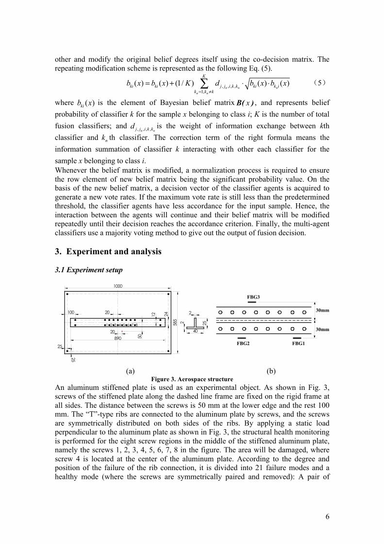
(a) (b) Figure 3. Aerospace structure
An aluminum stiffened plate is used as an experimental object. As shown in Fig. 3,
screws of the stiffened plate along the dashed line frame are fixed on the rigid frame at
all sides. The distance between the screws is 50 mm at the lower edge and the rest 100
mm. The “T”-type ribs are connected to the aluminum plate by screws, and the screws
are symmetrically distributed on both sides of the ribs. By applying a static load
perpendicular to the aluminum plate as shown in Fig. 3, the structural health monitoring
is performed for the eight screw regions in the middle of the stiffened aluminum plate,
namely the screws 1, 2, 3, 4, 5, 6, 7, 8 in the figure. The area will be damaged, where
screw 4 is located at the center of the aluminum plate. According to the degree and
position of the failure of the rib connection, it is divided into 21 failure modes and a
healthy mode (where the screws are symmetrically paired and removed): A pair of
7
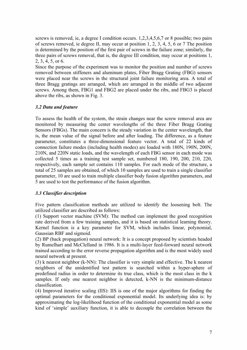
screws is removed, ie, a degree I condition occurs. 1,2,3,4,5,6,7 or 8 possible; two pairs
of screws removed, ie degree II, may occur at position 1, 2, 3, 4, 5, 6 or 7 The position
is determined by the position of the first pair of screws in the failure zone; similarly, the
three pairs of screws removal, that is, the degree III condition, may occur at positions 1,
2, 3, 4, 5, or 6.
Since the purpose of the experiment was to monitor the position and number of screws
removed between stiffeners and aluminum plates, Fiber Bragg Grating (FBG) sensors
were placed near the screws in the structural joint failure monitoring area. A total of
three Bragg gratings are arranged, which are arranged in the middle of two adjacent
screws. Among them, FBG1 and FBG2 are placed under the ribs, and FBG3 is placed
above the ribs, as shown in Fig. 3.
3.2 Data and feature
To assess the health of the system, the strain changes near the screw removal area are
monitored by measuring the center wavelengths of the three Fiber Bragg Grating
Sensors (FBGs). The main concern is the steady variation in the center wavelength, that
is, the mean value of the signal before and after loading. The difference, as a feature
parameter, constitutes a three-dimensional feature vector. A total of 22 kinds of
connection failure modes (including health modes) are loaded with 180N, 190N, 200N,
210N, and 220N static loads, and the wavelength of each FBG sensor in each mode was
collected 5 times as a training test sample set, numbered 180, 190, 200, 210, 220,
respectively, each sample set contains 110 samples. For each mode of the structure, a
total of 25 samples are obtained, of which 10 samples are used to train a single classifier
parameter, 10 are used to train multiple classifier body fusion algorithm parameters, and
5 are used to test the performance of the fusion algorithm.
3.3 Classifier description
Five pattern classification methods are utilized to identify the loosening bolt. The
utilized classifier are described as follows:
(1) Support vector machine (SVM): The method can implement the good recognition
rate derived from a few training samples, and it is based on statistical learning theory.
Kernel function is a key parameter for SVM, which includes linear, polynomial,
Gaussian RBF and sigmoid.
(2) BP (back propagation) neural network: It is a concept proposed by scientists headed
by Rumelhart and McClelland in 1986. It is a multi-layer feed-forward neural network
trained according to the error reverse propagation algorithm and is the most widely used
neural network at present.
(3) k nearest neighbor (k-NN): The classifier is very simple and effective. The k nearest
neighbors of the unidentified test pattern is searched within a hyper-sphere of
predefined radius in order to determine its true class, which is the most class in the k
samples. If only one nearest neighbor is detected, k-NN is the minimum-distance
classification.
(4) Improved iterative scaling (IIS): IIS is one of the major algorithms for finding the
optimal parameters for the conditional exponential model. Its underlying idea is: by
approximating the log-likelihood function of the conditional exponential model as some
kind of ‘simple’ auxiliary function, it is able to decouple the correlation between the

8
parameters and search for the maximum point along many directions simultaneously.
By carrying out this procedure iteratively, the approximated optimal point found over
the ‘simplified’ function is guaranteed to converge to the true optimal point due to the
convexity of the objective function.
(5) Gaussian mixture model (GMM): The classifier is based on Gaussian component
functions. The linear combination of Gaussian functions is capable of representing a
large class of the sample distribution. In principle, it is a compromise between the
performance and the complexity. Gaussian mixture has remarkable capability to model
the irregular data.
3.4 Selection of classifiers
Based on the individual classification decisions acquired in the first step, the spare
dynamic classifier selection method introduced in Section 2.2. It is used for less number
selection of classifier in five classifiers. The optimized selected results for different
numbers of classifiers and the fusion accuracy are shown in Table 1. The results show
the fusion accuracy rate with the less selection classifier group is higher than that of the
one with more classifiers. Therefore, selection of classifiers is proposed as a potential
optimization process before the final decision fusion.
Table 1. Atom k-NN sample set dynamic classifier selection
Atom GMM BP knn SVM IIS Classifier
Number
Fusion
Accuracy
1 √ √ √ √ √ 5 1.000
2 √ √ √ √ √ 5 1.000
9 √ √ 2 0.6777
10 √ √ 2 1.000
17 √ √ √ 3 1.000
18 √ √ √ 3 1.000
70 √ √ 2 0.6777
95 √ 1 1.000
3.5 Decision fusion
After the classifiers are selected, for different fused classifier group, multi- classifiers
are fused using multi agent methods. In the multi-agent method, accordance criterion is
a vital parameter. Multi-agent fusion result based on sparse dynamic classifier selection
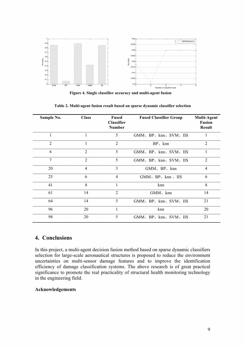
are shown in Table 2. In Fig 4. the results show the accuracy of the single classifier and
the proposed dynamic fusion method, and the fusion rate with the less selection
classifier group is higher than that of the one with more classifiers. Therefore, dynamic
selection of classifiers is proposed as a potential optimization process before the final
decision fusion.
9
SVM BP kNN GMM IIS0
0.1
0.2
0.3
0.4
0.5
0.6
0.7
0.8
0.9
1
Accuracy
1 2 3 4 5
0.9
0.905
0.91
0.915
0.92
0.925
0.93
0.935
0.94
Number of classifier fused
Accura
cy
MASSelection
Figure 4. Single classifier accuracy and multi-agent fusion
Table 2. Multi-agent fusion result based on sparse dynamic classifier selection
4. Conclusions
In this project, a multi-agent decision fusion method based on sparse dynamic classifiers
selection for large-scale aeronautical structures is proposed to reduce the environment
uncertainties on multi-sensor damage features and to improve the identification
efficiency of damage classification systems. The above research is of great practical
significance to promote the real practicality of structural health monitoring technology
in the engineering field.
Acknowledgements
Sample No. Class Fused
Classifier
Number
Fused Classifier Group Multi-Agent
Fusion
Result
1 1 5 GMM、BP、knn、SVM、IIS 1
2 1 2 BP、knn 2
6 2 5 GMM、BP、knn、SVM、IIS 1
7 2 5 GMM、BP、knn、SVM、IIS 2
20 4 3 GMM、BP、knn 4
25 6 4 GMM、BP、knn 、IIS 6
41 8 1 knn 8
61 14 2 GMM、knn 14
64 14 5 GMM、BP、knn、SVM、IIS 21
96 20 1 knn 20
98 20 5 GMM、BP、knn、SVM、IIS 21
10
This work is supported by the National Natural Science Foundation of China (Grant no.
51405409) and the Fundamental Research Funds for the Central Universities
(2018B04514).
References
1. Sakai T, et al, “Bolt clamping force measurement with ultrasonic waves”,
Transactions of the Japan Society of Mechanical Engineers 43, pp 723-29, 1977.
2. Gotoh Y, et al, “Study on inspection method to measure slack of a bolt using
electromagnetic vibration”, Journal of the Japanese Society for Non-Destructive
Inspection 51, pp 24-31, 2002.
3. Nai N, Hess D, “Experimental study of loosening of threaded fasteners due to
dynamic shear loads” , J. Sound Vib. 253(3), pp 585-602, 2003.
4. Caccese V, Mewer R, Vel S S, “Detection of bolt load loss in hybrid
composite/metal bolted connections”, Eng. Struct. 26, pp 895-906, 2004.
5. Brown R L, Adams D E, “Equilibrium point damage prognosis models for
structural health monitoring”, J. Sound Vib. 262, pp 591-611, 2003.
6. Todd M D, Nichols J M, Nichols C J,Virgin L N, “An assessment of modal
property effectiveness in detecting bolted joint degradation: theory and
experiment”, J. Sound Vib. 275, pp 1113-26, 2004.
7. Nichols J, Todd M, Wait J, “Using state space predictive modeling with chaotic
interrogation in detecting joint preload loss in a frame structure”, Smart Mater.
Struc. 12, pp 580-601, 2003.
8. Nichols J, Nichols C, Todd M, Seaver M and Trickey S, “Use of data driven phase
space models in assessing the strength of a bolted connection in a composite
beam”, Smart Mater. Struct. 13, pp 241-50, 2004.
9. Moniz L, Nichols J M, Nichols C J, Seaver M, Trickey S T, Todd M D, Pecora L
M, Virgin L N, “A multivariate, attractor-based approach to structural health
monitoring”, J. Sound Vib. 283, pp 295-310, 2005.
10. Rutherford A C, Park G, Farrar C R, “Non-linear feature identifications based on
self-sensing impedance measurements for structural health assessment”, Mech.
Syst. Signal Pr. 21, pp 322-33, 2007.
11. Milanese A, Marzocca P, Nichols J M, Seaver M, Trickey S T, “Modeling and
detection of joint loosening using output-only broad-band vibration data”, Struct.
Health Monit. pp 309-28, 2008.
12. Derek Doyle, Andrei Zagrai, Brandon Arritt, Hakan Çakan, “Damage detection in
bolted space structures”, J. Intel. Mat. Syst. Str. 21, pp 251-64, 2010.
13. Grady I Lemoine, Kevin W Love, Todd A Anderson, “An electric potential-based
structural health monitoring technology using neural network”, In : Fu-Kuo
Chang. Proceedings of the 4th International Workshop on Structural Health
Monitoring. Stanford, CA, USA: DEStech Publications pp 387-95, 2003.
14. Zhao X, Kwan C, Xu R, Qian T, Hay T, Rose J L, Raju B B, Maier R, Hexemer R
“Non-destructive inspection of metal matrix composites using guided waves in
Review of Quantitative Nondestructive Evaluation”, Vol. 23, D. O. Thompson and
D. E. Chimenti, eds, American Institute of Physics, Melville, NY, 914-20, 2004.
15. D. L. Donoho, “Compressed sensing”, IEEE T. Inform. Theory 52, pp 1289-1306,
2006.